Big Data Small Footprint: The Design of A Low-Power ...infolab.stanford.edu/~echang/BigDataSmallFootprint-VLDB-2014.pdf · Classifier for Detecting Transportation Modes Meng-Chieh

Big Data Small Footprint: The Design of A Low-PowerClassifier for Detecting Transportation Modes

Meng-Chieh Yu ∗

HTC, TaiwanMengchieh [email protected]

Tong Yu ∗

National Taiwan [email protected]

Shao-Chen WangHTC, Taiwan

Daniel.SC [email protected]

Chih-Jen LinNational Taiwan [email protected]

Edward Y. ChangHTC, Taiwan

Edward [email protected]

ABSTRACTSensors on mobile phones and wearables, and in general sen-sors on IoT (Internet of Things), bring forth a couple of newchallenges to big data research. First, the power consump-tion for analyzing sensor data must be low, since most wear-ables and portable devices are power-strapped. Second, thevelocity of analyzing big data on these devices must be high,otherwise the limited local storage may overflow.

This paper presents our hardware-software co-design ofa classifier for wearables to detect a person’s transporta-tion mode (i.e., still, walking, running, biking, and on avehicle). We particularly focus on addressing the big-datasmall-footprint requirement by designing a classifier that islow in both computational complexity and memory require-ment. Together with a sensor-hub configuration, we areable to drastically reduce power consumption by 99%, whilemaintaining competitive mode-detection accuracy. The dataused in the paper is made publicly available for conductingresearch.

Categories and Subject DescriptorsI.5.2 [Pattern Recognition]: Design Methodology-classifierdesign and evaluation

General TermsAlgorithms, Design, Experimentation, Measurement

KeywordsSensor hub, Big data small footprint, Context-aware com-puting, Transportation mode, Classification, Support vectormachines

∗These two authors contributed equally.

Permission to make digital or hard copies of all or part of this work forpersonal or classroom use is granted without fee provided that copies arenot made or distributed for profit or commercial advantage and that copiesbear this notice and the full citation on the first page. To copy otherwise, torepublish, to post on servers or to redistribute to lists, requires prior specificpermission and/or a fee. Articles from this volume were invited to presenttheir results at the 40th International Conference on Very Large Data Bases,September 1st - 5th, 2014, Hangzhou, China. Proceedings of the VLDBEndowment, Vol. 7, No. 13Copyright 2014 VLDB Endowment 2150-8097/14/05...$15.00.

1. INTRODUCTIONThough cloud computing promises virtually unlimited re-

sources for processing and analyzing big data [6], voluminousdata must be transmitted to a data center before taking allthe advantages of cloud computing. Unfortunately, sensorson mobile phones and wearables come up against both mem-ory and power constraints to effectively transmit or analyzebig data. In this work, via the design of a transportation-mode detector, which extracts and analyzes motion-sensordata on mobile and wearable devices, we illustrate the crit-ical issue of big data small footprint, and propose strategiesin both hardware and software to overcome such resource-consumption issue.

Detecting transportation modes (such as still, walking,running, biking, and on a vehicle) of a user is a critical sub-routine of many mobile applications. The detected modecan be used to infer the user’s state to perform context-aware computing. For instance, a fitness application usesthe predicted state to estimate the amount of calories burnt.A shopping application uses the predicted state to infer ifa user is shopping or dinning when she/he wanders in frontof a shop or sits still at a restaurant. Determining a user’stransportation mode requires first collecting movement datavia sensors, and then classifying the user’s state after pro-cessing and fusing various sensor signals. Though manystudies (see Section 2) have proposed methods for detectingtransportation modes, these methods often make unrealis-tic assumptions of unlimited power and resources. Severalapplications have been launched to do the same. However,all these applications are power hogs, and cannot be turnedon all the time to perform their duties. For instance, thesensors used by Google Now [13] on Android phones con-sume around 100mA, and thus forces most users to turn thefeature off. Similarly, processing sensor data on wearables1

must minimize power consumption in order to lengthen theoperation time of the hosting devices.

To minimize power consumption and memory require-ment, we employ both hardware and software strategies.Though this paper’s focus is on reducing the footprint ofa big-data classifier, we present the entire solution stack forcompleteness. Our presentation first reveals bottlenecks andthen accurately accounts for each strategy’s contribution.Specifically on the challenges that are relevant to the big-

1The capacity of a battery on a typical wearable, e.g.,Sony/Samsung watch, is under 315mAh [27].

1

data community, we employ the following four strategies totackle them:• Big data. The more data that can be collected, the more

accurate a classifier can be trained.• Small footprint. The computational complexity of a clas-

sifier should be low, and preferably independent of thesize of training data. At the same time, model complex-ity must remain robust to maintain high classification ac-curacy. Tradeoffs between model complexity and compu-tational complexity are carefully studied, experimented,and analyzed.• Data substitution. When the data of a low power-consuming

sensor can substitute that of a higher one, the higherpower-consuming sensor can be turned off, thus conserv-ing power. Specifically, we implement a virtual gyroscopesolution using the signals of an accelerometer and a mag-netometer, which together consumes 8% power comparedwith using the signals of a physical gyroscope (see Table 1for power specifications).• Multi-tier design. We design a multi-tier framework, which

uses minimal resources to detect some modes, and in-creases resource consumption only when between-modeambiguity is present.By carefully considering trade-offs between model com-

plexity and computational complexity, and by minimizingresource requirement and power consumption (via hardware-software co-design and reduction of the classifier’s footprint),we reduce power consumption by 99% (from 88.5mA to0.73mA), while maintaining 92.5% accuracy in detecting fivetransportation modes.

The rest of the paper is organized as follows: Section 2presents representative related work. Section 3 depicts fea-ture selection, classifier selection, and our error-correctionscheme. In Section 4, we present the design of a smallfootprint classifier for a low-power sensor hub. In addition,we propose both a virtual gyroscope solution and multi-tierframework to further reduce power consumption. Section 5outlines our data collection process and reports various ex-perimental results. The transportation-mode data is madeavailable at [15] for download. We summarize our contribu-tions and offer concluding remarks in Section 6.

2. RELATED WORKPrior studies on transportation-mode detection can be

categorized into three approaches: location-based, motion-sensor-based, and hybrid. The key difference of our work isthat we address the practical issue of resource consumption.

2.1 Location-Based ApproachThe location-based approach is the most popular one for

detecting transportation modes. This is because sensorssuch as GPS, GSM, and WiFi are widely available on mobilephones. In addition, the location and changing speed canconveniently reveal a user’s means of transportation.

The method of using the patterns of signal-strength fluc-tuations and serving-cell changes to identify transportationmodes is proposed by [2]. The work achieves 82% accuracyin detecting among modes of still, walk, and on a vehicle.For the usage of GSM data, the study of [26] extracts mobil-ity properties from a coarse-grained GSM signal to achieve85% accuracy for detecting among the same three modes.The work of [35] extracts heading change rate, velocity, andacceleration from GPS signals to predict the modes of walk,

Table 1: Power consumption of processors and sen-sors. The active status indicates that only ourtransportation-mode algorithm is running.

Power ConditionCPU (running at 1.4GHz) 88.0mA Active status

5.2mA Idle statusMCU (running at 16MHz) 0.5mA Active status

0.1mA Idle statusGPS 30.0mA Tracking satelliteWiFi 10.5mA Scanning every 10 secGyroscope 6.0mA Sampling at 30HzMagnetometer 0.4mA Sampling at 30HzAccelerometer 0.1mA Sampling at 30Hz

bike, driving, and bus. Recent work of [30] uses GPS andknowledge of the underlying transportation network includ-ing real time bus locations, spatial rail and spatial bus stopinformation to achieve detection accuracy of 93%.

Unfortunately, the location-based approach suffers fromhigh power consumption and can fail in environments wheresome signals are not available (e.g., GPS signals are notavailable indoors). Table 1 lists power consumption of pro-cessors and sensors. It is evident that both GPS and WiFiconsume significant power, and when they are employed,the power consumption is not suitable for devices such aswatches and wrist bands, whose 315mA batteries last lessthan half a day when only the GPS is on.

2.2 Sensor-Based ApproachThe motion-sensor-based approach is mostly used to de-

tect between walking and running in commercial productssuch as Fuelband [22], miCoach [1], and Fitbit [9]. The studyof [31] uses an accelerometer to detect six typical transporta-tion modes, and concludes that the acceleration synthesiza-tion based method outperforms the acceleration decomposi-tion based method. The research of [34] extracts orientation-independent features from vertical and horizonal compo-nents and magnitudes from the signals of an accelerom-eter. Combined with error correction methods using k-means clustering and HMM-based Viterbi algorithm, thiswork achieves 90% accuracy for classifying six modes.

2.3 Hybrid Location/Sensor-Based ApproachFor the location-based and motion-sensor-based hybrid

approach, the studies of [32], [25], and [17] employ bothGPS and accelerometer signals to detect the transporta-tion mode. In addition, [18] proposes an adaptive sensingpipeline, which switches the depth and complexity of signalprocessing according to the quality of the input signals fromGPS, an accelerometer, and a microphone. However, theseschemes all suffer from high power consumption.

2.4 Resource ConsiderationThe tasks of sensor-signal sampling, feature extraction,

and mode classification are continuously run to consume re-sources. Some prior works address the problem of powerconsumption via signal subsampling and process admissioncontrol. The studies of [24] focus on adapting the samplingrate to extract sensor signals. The data admission controland duty cycling strategies are proposed by [18]. The workof [28] presents a framework that reduces the need of running

2

Table 2: Representative work of transportation-mode detection (accuracy in percentage). Note thatAcc means accelerometer and mic means micro-phone in this table.Ref # Modes Sensors Used Accuracy Power[2] 3 GSM 82.00% not considered[26] 3 GSM 84.73% not considered[35] 4 GPS 76.20% not considered[30] 6 GPS, GIS 93.50% not considered[20] 3 GSM, WiFi 88.95% not considered[31] 6 Acc. 70.73% not considered[34] 6 Acc. 90.60% not considered[32] 4 Acc., GPS 91.00% not considered[18] 5 Acc., GPS, mic. 95.10% 20.5mA[25] 5 Acc., GPS, GSM 93.60% 15.1mA

the main recognition system and can still maintain compet-itive accuracy. The work of [21] reduces power consumptionby inferring unknown context features from the relationshipbetween various contexts.

Our work provides resource management in both hard-ware and software, and achieves much more significant re-source conservation compared with all prior approaches. Ourdesign uses MCU to replace CPU, and low-power sensorssuch as accelerometer and magnetometer to replace GPS,WiFi, and gyroscope. Furthermore, the small footprint ofour classifier reduces both memory requirement and powerconsumption.

Table 2 summarizes representative schemes mentioned inthis section, including signal sources, number of detectionmodes, accuracy, and power consideration. (Note that ac-curacy values in these studies are obtained upon differentdatasets and experimental environments.) Most schemesdo not address the power consumption issue. The onesthat consider the power issue consume at least 20 times(15.1mA achieved by [25] vs. 0.73mA by ours) our proposedhardware-software co-design.

3. ARCHITECTUREThis section presents our transportation-mode detection

architecture, of which the design goal is to achieve high de-tection accuracy at low power consumption. The architec-ture consists of computation modules located at sensor hub,mobile client, and cloud server. The sensor hub employslow-power components and makes a preliminary predictionon a user’s transportation mode. The mobile client andcloud server then use additional information (e.g., locationinformation, map, and transit route), if applicable, to fur-ther improve prediction accuracy. The three tiers work intandem to adapt to available resources and power. In thispaper, we particularly focus on depicting our design andimplementation of a low-power, low-cost sensor hub.

The overall structure of the transportation-mode detec-tion system on the sensor hub is depicted in Figure 1, whichshows source sensors on the left-hand side and five targetmodes on the right-hand side. The hub employs an MCU(operating at speeds up to 72MHz), which has power con-sumption of 0.1mA while running at 16MHz, compared to88.5mA of a 1.4GHz Quad-core CPU. The hub is configuredwith three motion sensors: an accelerometer, a gyroscope,and a magnetometer, all running at 30Hz sampling rate.

Figure 1: Structure of overall system.

Predicting transportation mode consists of three key steps:feature extraction, mode classification, and error correction.The mode classifier is trained offline via a training pipeline,details of which are presented in Section 3.2. Once signalshave been collected from the sensors, the hub first extractsessential features. It then inputs the features to the classi-fier to determine the transportation mode. In the end, thehub performs an error correction scheme to remove noise. Inthis work, our target transportation modes are: still, walk-ing, running, biking, and (on) vehicle. We use symbols Still,Walk, Run, Bike, and Vehicle to denote these modes, respec-tively. Note that the Vehicle mode includes motorcycle, car,bus, metro, train, and high speed rail (HSR).

The remainder of this section describes these three onlinesteps.

3.1 Feature ExtractionOur sensor hub uses 3-axis motion sensors. An accelerom-

eter is an electromechanical device measuring accelerationforces in three axes. By sensing the amount of dynamic ac-celeration, a subroutine can analyze the way the device ismoving in three dimensions. A gyroscope measures angu-lar velocity in three axes. The output of a gyroscope tellsdevice rotational velocity in three orthogonal axes. Since asensor hub may be mounted on a mobile device in a tiltedangle, and that device can be carried by the user in any ori-entation, it is not productive to consider acceleration valuesin three separate axes. Instead, for the purpose of discern-ing transportation modes, the magnitude of acceleration, orthe energy of motion, is essential. Therefore we combinesignals from the three axes as the basis of the magnitudefeature. For example, the magnitude of the accelerometeris Amag =

√(Ax)2 + (Ay)2 + (Az)2. The same calculation

is used for signals from the gyroscope and magnetometer.This formulation enables our system to assume a randomorientation and position of a device for mode prediction.

In addition, the magnitude measured at a time instant isnot a robust feature. We thus aggregate signals in a movingwindow, and extract features from each window. We eval-uated the performance by using different window sizes, andfinally determined 512 as the choice because it yielded themost suitable result. (Section 5.2.1 presents the detailedevaluation.) Extracted features can be classified into twocategories, including a category in the time domain and theother in the frequency domain. According to experience ofprior works, we tried 22 features in the time-domain, and 8

3

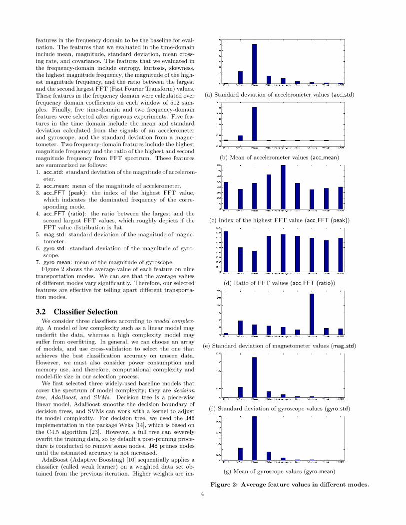
features in the frequency domain to be the baseline for eval-uation. The features that we evaluated in the time-domaininclude mean, magnitude, standard deviation, mean cross-ing rate, and covariance. The features that we evaluated inthe frequency-domain include entropy, kurtosis, skewness,the highest magnitude frequency, the magnitude of the high-est magnitude frequency, and the ratio between the largestand the second largest FFT (Fast Fourier Transform) values.These features in the frequency domain were calculated overfrequency domain coefficients on each window of 512 sam-ples. Finally, five time-domain and two frequency-domainfeatures were selected after rigorous experiments. Five fea-tures in the time domain include the mean and standarddeviation calculated from the signals of an accelerometerand gyroscope, and the standard deviation from a magne-tometer. Two frequency-domain features include the highestmagnitude frequency and the ratio of the highest and secondmagnitude frequency from FFT spectrum. These featuresare summarized as follows:1. acc std: standard deviation of the magnitude of accelerom-

eter.2. acc mean: mean of the magnitude of accelerometer.3. acc FFT (peak): the index of the highest FFT value,

which indicates the dominated frequency of the corre-sponding mode.

4. acc FFT (ratio): the ratio between the largest and thesecond largest FFT values, which roughly depicts if theFFT value distribution is flat.

5. mag std: standard deviation of the magnitude of magne-tometer.

6. gyro std: standard deviation of the magnitude of gyro-scope.

7. gyro mean: mean of the magnitude of gyroscope.Figure 2 shows the average value of each feature on nine

transportation modes. We can see that the average valuesof different modes vary significantly. Therefore, our selectedfeatures are effective for telling apart different transporta-tion modes.

3.2 Classifier SelectionWe consider three classifiers according to model complex-

ity. A model of low complexity such as a linear model mayunderfit the data, whereas a high complexity model maysuffer from overfitting. In general, we can choose an arrayof models, and use cross-validation to select the one thatachieves the best classification accuracy on unseen data.However, we must also consider power consumption andmemory use, and therefore, computational complexity andmodel-file size in our selection process.

We first selected three widely-used baseline models thatcover the spectrum of model complexity; they are decisiontree, AdaBoost, and SVMs. Decision tree is a piece-wiselinear model, AdaBoost smooths the decision boundary ofdecision trees, and SVMs can work with a kernel to adjustits model complexity. For decision tree, we used the J48implementation in the package Weka [14], which is based onthe C4.5 algorithm [23]. However, a full tree can severelyoverfit the training data, so by default a post-pruning proce-dure is conducted to remove some nodes. J48 prunes nodesuntil the estimated accuracy is not increased.

AdaBoost (Adaptive Boosting) [10] sequentially applies aclassifier (called weak learner) on a weighted data set ob-tained from the previous iteration. Higher weights are im-

(a) Standard deviation of accelerometer values (acc std)

(b) Mean of accelerometer values (acc mean)

(c) Index of the highest FFT value (acc FFT (peak))

(d) Ratio of FFT values (acc FFT (ratio))

(e) Standard deviation of magnetometer values (mag std)

(f) Standard deviation of gyroscope values (gyro std)

(g) Mean of gyroscope values (gyro mean)

Figure 2: Average feature values in different modes.

4

posed on wrongly predicted data in previous iterations. Thisadaptive setting is known to mitigate overfitting. We con-sidered J48 as the weak learner and applied the AdaBoostimplementation in Weka. The number of iterations was cho-sen to be 10, so 10 decision trees are included in the model.

Support vector machines (SVMs) [3, 8] can efficiently per-form a non-linear classification using the kernel trick, im-plicitly mapping data in the input space onto some high-dimensional feature spaces. It is known that SVMs are sen-sitive to the numeric range of feature values. Furthermore,some features in our data have values in a very small range.Therefore, we applied a log-scaling technique to make valuesmore evenly distributed. In addition, SVMs are also knownto be sensitive to parameter settings, so we conducted crossvalidation (CV) to select parameters. The SVM packageLIBSVM [5] was employed for our experiments.

SVMs were chosen to be our classifier because SVMs enjoythe highest mode-prediction accuracy. Section 5.2.3 presentsthe details of our classifier evaluation. When training datais abundant (in a big-data scenario), the large number ofsupport vectors can make the footprint of its model file quitelarge. In Section 4, we will address the issues of resourceconservation for SVMs to drastically reduce its footprint.

3.3 Error Correction via VotingIn transportation-mode detection, an incorrect detection

by a classifier may be caused by short-term changes of thetransportation mode. When an activity is changed from onemode (e.g., Walk) to another (e.g., Still), the moving windowthat straddles the two modes during transition can includefeatures from both modes. Therefore, the classification maybe erroneous. We propose a voting scheme to address thisproblem.

At time t− 1, the system maintains scores of all modes.

scoret−1(Still), scoret−1(Walk), . . . , scoret−1(Vehicle). (1)

Then at time t, the classifier predicts a label. This label andthe past scores in (1) are used together to update scores andmake mode predictions.

Figure 3 presents the pseudo code of the voting scheme.In the beginning, all of the scores are set as zero. At eachtime point, the score of the mode predicted by the classifieris increased by one unit. In contrast, the scores of the othermodes are decreased by one unit. The upper-bound of thescore is set as four units, whereas the lower bound zero.Then, the mode with the highest score is determined as themodified prediction. Section 5.2.4 presents the improvementin prediction accuracy achieved by this voting scheme.

4. RESOURCE CONSERVATIONAs presented in Section 1, we employ three strategies:

i) small footprint, ii) data substitution, and iii) multi-tierdesign, to conserve resources even though we use a large-pool of training instances. We present details in this section.

4.1 Small FootprintMoving CPU computation to a low-power MCU saves sig-

nificant power. However, that saving is not good enoughfor wearables, and we must save even more. At the sametime, the low-cost sensor hub demands us to design a small-footprint classifier that does not take up much memory space.

Algorithm 3.1: VotingScheme(cresult)

Inputcresult : the result detected by classifierOutputvresult : the result after voting scheme

max = cresultif prob[cresult] ≤ 4

then prob[cresult]← prob[cresult] + 1for i← 0 to classNum

do

if i 6= cresult and prob[i] ≤ 0

then prob[i]← prob[i]− 1if prob[max] ≤ prob[i]

then max← ivresult← max

Figure 3: Pseudo code of voting scheme.

A small footprint design of our classifier not only saves mem-ory space, but also reduces computation and thereby saveseven more power.

This section aims to reduce the model-file size of SVMs.Typically, employing the kernel trick provides higher modelcomplexity to the SVM classifier to yield higher classifica-tion accuracy. However, the kernel trick requires the formu-lation of a kernel matrix, the size of which depends on thesize of the training data. In the end of the training stage,the yielded support vectors are collected in a model file toperform class prediction on unseen instances. The size orfootprint of the model file typically depends on the size ofthe training data. In a big-data setting when a huge amountof training data is used to improve classification accuracy,the model file is inevitably large. Such consequence is notan issue when classification is performed in the cloud, whereboth memory and CPU are virtually unlimited. On our sen-sor hub, which is mounted on a low-power device, a largefootprint is detrimental.

Let us visit the formulation of SVMs in a binary classifica-tion setting. Support vector machines [3, 8] minimize the fol-lowing weighted sum of the regularization term and traininglosses for the given two-class training data (y1,x1), . . . (yl,xl).

minw,b

1

2wTw+C

∑l

i=1max(1− yi(wTφ(xi) + b), 0), (2)

where yi = ±1, ∀i are class labels, xi ∈ Rn, ∀i are trainingfeature vectors, and C is the penalty parameter. An impor-tant characteristic of SVMs is that a feature vector xi canbe mapped to a higher dimensional space via a projectionfunction φ(·) to improve class separability. To handle thehigh dimensionality of the vector variable w, we can applythe kernel method and solve the following dual optimizationproblem:

minα

1

2αTQα− eTα

subject to yTα = 0

0 ≤ αi ≤ C, i = 1, . . . , l,

(3)

where

Qij = yiyjφ(xi)Tφ(xj) = yiyjK(xi,xj), (4)

5

and K(xi,xj) is the kernel function. The optimal solutionsof the primal problem (2) and the dual problem (3) satisfythe following relationship (l denotes the number of traininginstances):

w =∑l

i=1αiyiφ(xi). (5)

The set of support vectors is defined to include xi with αi >0, since αi = 0 implies that xi is inactive in (5). Witha special φ(·) function, the kernel value K(xi,xj) can beeasily calculated even though it is the inner product of twohigh dimensional vectors. Let us consider the following RBF(Gaussian) kernel as an example.

K(xi,xj) = e−γ‖xi−xj‖2 ,

where γ is the kernel parameter. RBF kernel in fact mapsoriginal data to infinite dimensions, so the SVM model (5)also has infinite dimensions and cannot be saved directly. Inorder to save the model, all the support vectors xi and theircorresponding non-zero αi must be stored and then loadedinto memory when making predictions. If the number ofsupport vectors is O(l), then the O(ln) size of the model,where n is the number of features, can be exceedingly large.

In order to achieve extremely small model size, we proposean advanced setting by low-degree polynomial mappings ofdata [7] when storing the model. From (4), every valid kernelvalue is the inner product between two vectors. We considerthe polynomial kernel

K(xi,xj) = (γxTi xj + 1)d = φ(xi)Tφ(xj),

where d is the degree. If n is the number of features, then

dimensionality of φ(x) =

(n+ d

n

).

For example, if d = 2, then

φ(x) = [1,√

2γx1, . . . ,√

2γxn, γx21, . . . ,

γx2n,√

2γx1x2, . . . ,√

2γxn−1xn]T .

Therefore, if the dimensionality of φ(x) is not too high, theninstead of storing the dual optimal solution and the supportvectors (i.e., all αi,xi with αi > 0), we only store (w, b) inthe model. To be more precise, if φ(x) is very high dimen-sional (possibly infinite dimensional), then w in (5) cannotbe explicitly expressed and we must rely on kernel tech-niques. In contrast, if φ(x) is low dimensional, then thevector w can be explicitly formed and stored. Because thelength of w is the same as that of φ(·), a nice property isthat the model size becomes independent of the number oftraining data. If we use the one-against-one strategy for k-class data (discussed later in this section) and assume single-precision storage, the model size is(

k

2

)× (length of w + 1)× 4bytes

=

(k

2

)×

((n+ d

d

)+ 1

)× 4bytes.

(6)

We hope that when using a small d (i.e., low-degree polyno-mial mappings),

(n+dd

)is smaller than O(ln) of using kernels

and the model size in (6) is smaller. Then we can simulta-neously reduce the model size and achieve nonlinear separa-bility. Take d = 3 as an example.(

n+ d

d

)≤ n3 � ln if n2 � l. (7)

Because the number of features (7 in our case) is small andin a big-data scenario, l can be in the order of millions, easilyn2 � l and saving in model size is significant.

Of course, to reduce the model size as small as possible, wecan simply set φ(x) = x so that the data is not mapped to adifferent space. The model size is very small because storingon (w, b) needs only n+ 1 float-point values, where n is thenumber of features in linear space. However, linear SVMs’result usually cannot match that of SVMs with kernel.

Usually, when the degree of polynomial mapping increases,the performance of the SVM classifier would become better.At the same time, the SVM model size would increase. Whatwe need to do is to find an appropriate d, which achievesa good balance between classification accuracy and modelsize. In Section 5.2.3, we report that degree-3 polynomialmappings achieves the best such balance.

We briefly discuss multi-class strategies because the num-ber of transportation modes is more than two. Both deci-sion tree and AdaBoost can directly handle multi-class data,but SVMs do not. Recall that in problem (2), yi = ±1 soonly data in two classes are handled. Here we follow LIB-SVM to use the one-against-one multi-class strategy [16].For k classes of data, this method builds a model for everytwo classes of training data. In the end k(k − 1)/2 mod-els are generated. Another frequently used technique formulti-class SVMs is the one-against-rest strategy [4], whichconstructs only k models. Each of the k models is trainedby treating one class as positive and all the rest as negative.Although the one-against-rest method has the advantage ofhaving fewer models,2 its performance may not be always asgood as or better than one-against-one [12]. From our ex-periments on mode detection, one-against-rest gives slightlylower accuracy, so we choose the one-against-one method forall subsequent SVM experiments.

For example, considering a five-class one-against-one SVMclassification problem, if the number of feature is 7 and thedegree of polynomial mapping 3, the dimensionality of φ(·)is(n+dd

)=(7+33

)= 120. After considering the bias term,

the number of dimensions is 121. With 5 × (5 − 1)/2 = 10binary SVM models, the model size would be 10×121×4 =4, 840bytes = 4.84KB, which is smaller than the sensor hub’slimit of 16KB, satisfying the memory constraint.

Another merit of our polynomial SVM model is that itrequires low computational complexity when making pre-dictions, compared with what RBF kernel SVMs do. It isespecially important when the device’s computing capacityis not that high. Instead of computing the decision value by

f(x) =∑l

i=1,i6=0αiyiK(xi,x) + b, (8)

our method calculates the decision value simply by f(x) =wTφ(x) + b. Therefore, for data with number of instances

2If using the one-against-rest multi-class strategies, only krather than

(k2

)vectors of (w, b) must be stored.

6

Figure 4: Comparison of the mean and standard de-viation in each window from gyro and virtual gyro.

l and dimensions n, compared to the computational com-plexity O(ln) depicted in (8),3 the computational time aswell power is significantly reduced following a similar reasonexplained in (7).

4.2 Virtual Gyroscope SolutionA gyroscope is a device for measuring orientation, based

on the principles of angular momentum. In our feature se-lection experiment shown in Table 5, we can see that thefeatures of gyro std and gyro mean perform well especiallyfor the mode of Bike.

However, the gyroscope takes up about 85% of the totalpower consumption (i.e., about 7.0mA per hour under thesensor hub environment, reported in Section 5.3.1). To fur-ther reduce power consumption, we apply a method calledvirtual gyroscope to simulate the data of the gyroscope fromthat of the accelerometer and magnetometer combined.

In the procedure of a virtual gyroscope, we first pass ac-celerometer data into a low-pass filter to extract the gravityforce. Then, a mean filter is applied to both gravity-forceand magnetometer data to reduce noise. After that, the ro-tation matrix, which transforms gravity-force and magneticdata from the device’s coordinate system to the world’s co-ordinate system, is computed. Finally, with the idea in [29],the angular velocity ω can be obtained by the following equa-tion:

ω =dR(t)

dtRT (t) =

1

∆t(I −R(t− 1)RT (t)),

where R(t) is the rotation matrix at time t and ∆t is the timedifference. The virtual gyroscope data can be calculatedusing two consecutive rotation matrices and their recorded-time difference.

In this study, the features generated by the gyroscope in-clude gyro std and gyro mean. Figure 4 shows the compari-son of the mean and standard deviation features extractedfrom the physical and virtual gyroscope. The data in thefigure show that though the physical and virtual gyroscopedo not produce identical values, their spiking patterns arein tandem. The virtual gyroscope can achieve the samemode-prediction accuracy as the physical gyroscope at re-duced power consumption. The overall evaluation of powerconsumption and test accuracy is shown in Section 5.3.2.

4.3 A Two-Tier FrameworkThe goal of our detector is to identify the modes of Still,

Walk, Run, Bike, and Vehicle. However, a device is often

3Assume the number of support vectors is O(n).

Figure 5: The comparisons of acc std in still and fivevehicle modes. Two conditions are considered forStill: the phone is on the body or not. Two condi-tions are considered for five Vehicle modes: the Vehicleis stationary or moving.

placed on a stationary surface. For instance, a phone isplaced on a desk at home or at work in order to charge itsbattery. Such fully still mode indicates that a device is at astationary place affected by nothing but the gravity. (Notethat the fully still mode is a special case of the mode of Still.)If a simple rule can be derived to determine the fully stillmode, the system will only need to extract a small numberof relevant features to efficiently confirm its being in fullystill. In other words, it is not necessary to activate the fullmode-classification procedure at all times.

We would like to find a value of acc std, beneath which wecan safely classify the mode to be fully still without extract-ing features and running the classifier. Since from Figure 2we can observe that acc std is significantly smaller in modeStill than in modes Walk, Run, and Bike, we only had toexamine acc std between modes Still and Vehicle.

Figure 6: A hierarchical setting of transportation-mode detection.

Next, we observe the acc std value in the different vehi-cle modes including motorcycle, car, bus, metro, and highspeed rail (HSR). In addition, we monitor two conditionsof these vehicles, including stationary Vehicle and movingVehicle. Figure 5 compares the acc std values in Still andfive Vehicle modes. The results show that value of acc std islower than 0.06 except for in the motorcycle mode when theVehicle is stationary (e.g., stopping at a traffic light). Thus,we can set 0.06 as the threshold of the two-tier framework.An ultra-low-power microchip inside the accelerometer con-stantly collects data and directly predicts the Still modewhen the movement of the phone is insignificant. When

7

the accelerometer detects movement, it activates the proces-sor on the sensor hub to run the full feature-extraction andclass-prediction pipeline. Figure 6 depicts the framework,where the upper-left component activates feature extractionand mode classification according to the following rule:

If acc std ≤ 0.06predict mode Still

Elsepredict a mode by the transportation-mode classifier

5. EMPIRICAL STUDYDuring the design of our transportation-mode classifier,

we evaluated several feature-set and model alternatives. Thissection documents all evaluation details, divided into threesubsections: experiment setup, parameter and classifier se-lection, and resource conservation.

5.1 Experiment SetupThis subsection describes the details of experiment envi-

ronment, and training data collection.

5.1.1 Hardware & SoftwareAs a testing platform, we used the HTC One mobile phone,

which runs Android system. HTC One is equipped witha sensor hub, which consists of an ARM Cortex-M4 32-bit MCU (operating at speeds up to 72MHz), 32KB RAM,128KB flash, and three motion sensors: an accelerometer,a magnetometer, and a gyroscope. The processor of thesensor hub also supports digital signal processing (DSP) toenhance the processing performance for complex mathemat-ical computations, such as FFT. It also supports fixed-pointprocessing to optimize the usage of memory and computingtime. To evaluate different parameter settings of candidateclassifiers, the Weka Machine Learning tool [14] and LIBSVMlibrary [5] were employed. To evaluate the power consump-tion, we used Monsoon power monitor [19].

5.1.2 Data CollectionTable 3 shows the amount and distribution of the move-

ment data that we have collected since 2012. The 8, 311hours of 100GB data were collected via two avenues: ouruniversity program with 150 participating students, and agroup of 74 employees and interns. We made sure thatthe pool of participants sufficiently covered different genders(60% male), builds, and ages (20 to 63 years old). We im-plemented a data collection Android application for partici-pants to register their transportation status into ten modes:Still, Walk, Run, Bike, (riding) Motorcycle, Car, Bus, Metro,Train, and high speed rail (HSR). In our system design, wecombine modes of motorcycle, car, bus, metro, train, andHSR into the Vehicle mode. Experiments were conductedthrough splitting the data from the internal program intotraining and testing sets.

Because the class of Vehicle includes several transporta-tion modes and contains much more data instances than theother modes, we randomly sampled 25% of the Vehicle datato conduct training for avoiding the potential prediction biascaused by imbalanced data [33]. Because of the randomnessnature in the sampling process, we prepared ten (training,test) pairs for experiments and averaged the results of ourten runs on all experiments.

Table 3: Data collection time (hours) and mode dis-tribution.

Internal Program University ProgramStill 107 1,750Walk 121 1,263Run 61 88Bike 78 61Motorcycle 134 1,683Car 209 558Bus 69 1,248Metro 95 289Train 67 267HSR 91 72Total 1,031 7,280

Table 4: Window size selection. The test accuracy,memory usage, and response time are compared.

PerformanceWindow size

256 512 1,024 2,048

Accuracy 89.51 90.66 91.55 91.69Memory usage (KB) 1 2 4 8Response time (sec) 8.5 17.1 34.1 68.3Latency (50% overlap) 4.3 8.6 17.1 34.2

5.2 Parameter and Classifier SelectionExperiments were conducted to set feature-extraction win-

dow size, select most effective features, and evaluate threecandidate classifiers under various parameter settings.

5.2.1 Window SizeDifferent window sizes affect classification accuracy, re-

sponse time (latency), and memory size. Too small a win-dow may admit noise, and too large a window may overlysmooth out the data. We relied on cross-validation to selecta window size that achieves a reasonable tradeoff betweenthe three factors. Besides accuracy, response time affectsuser experience, as the larger the window size, the longerthe latency for a user to perceive a mode change. Sincethe sampling rate of sensors is at 30Hz, a window size of2, 048 takes over a minute to collect and then generate FFTfeatures. Though we employ a 50% window overlappingscheme, an over half-a-minute latency is not an acceptableuser experience. We consider an acceptable latency to beunder ten seconds.

Table 4 reports results of applying SVMs with a degree-3 polynomial mapping on four different window sizes (256,512, 1, 024, and 2, 048). The window sizes were selected as apower of two because of the FFT processing. Both sizes of512 and 1, 024 provide a reasonable response time and mode-prediction accuracy. Further increasing window size doesnot yield significant accuracy improvement (as expected),at the expense of long latency. We set the window size to be512 because of its lower latency of 8.6 seconds and relativelyhigh mode-prediction accuracy.

5.2.2 Feature SelectionFive features in the time domain (Ftime) and two fea-

tures in the frequency domain (Ffreq) were presented anddiscussed in Section 3.1. Here, we report our justification ofselecting those features.

We use two criteria for selecting features: effectivenessand cost. For effectiveness, we want to ensure that a feature

8

Table 5: Feature selection by using different fea-ture combinations. Ftime includes acc std, acc mean,mag std, gyro std, and gyro mean. F ′time includes acc std,acc mean, mag std. Ffreq includes acc FFT (peak) andacc FFT (ratio).

Still Walk Run Bike Vehicle AccuracyFtime 93.73 82.21 97.47 67.75 87.51 84.79Ftime+Ffreq 93.93 90.29 97.34 85.39 88.59 90.66F ′time+Ffreq 91.15 86.73 97.27 82.51 77.42 86.33

will be productive in improving mode-prediction accuracy.For cost, we want to make sure that a useful feature does notconsume too much power to extract or generate. There aretwo sources of cost: power consumed by a signal source andpower consumed by generating frequency-domain featuresvia FFT. A gyroscope consumes 6mA versus the 0.1mA con-sumed by an accelerometer and 0.4mA by a magnetometer.We would select frequency-domain features and gyroscopesignals only when they are proven to be productive.

We evaluated three sets of features:• Ftime: five time-domain features acc std, acc mean, mag std,

gyro std and gyro mean collected from accelerometer, mag-netometer, and gyroscope.• F ′time: three time-domain features acc std, acc mean, and

mag std collected from accelerometer and magnetometer.• Ffreq: two frequency-domain features acc FFT (peak) and

acc FFT (ratio), generated from accelerometer’s time-domainfeatures.Table 5 reports three sets of feature combinations. First,

it indicates that including frequency-domain features yieldsimproved accuracy. The second row of the table (Ftime+ Ffreq) yields 6.5 percentile improvement over the firstrow (five time-domain features), especially in predicting themodes of walk and bike. This result demonstrates that thefrequency-domain features are productive.

Since using a gyroscope consumes more than ten times thepower consumed when using an accelerometer and a mag-netometer, we evaluated the prediction degradation of re-moving the gyroscope. The third row of the table reports alower accuracy than the first two rows. This result presentsa dilemma: using the gyroscope is helpful but in order toconserve power, we should turn it off. Our solution to thisdilemma is devising a virtual gyroscope scheme, which sim-ulates physical gyroscope signals by an accelerometer and amagnetometer. We will report the good performance of thevirtual gyroscope shortly in Section 5.3.2.

5.2.3 Performance of ClassifiersTable 6 reports and compares classification accuracy and

confusion matrix for decision tree J48 (Weka default set-ting/with further pruning), AdaBoost (ten/three trees), andSVMs (RBF, degree-3 polynomial, and linear). The tableshows that the SVM (degree-3 polynomial) enjoys a muchhigher accuracy 90.66% over the 84.81% of decision tree(Weka default setting) and 87.16% of AdaBoost (ten trees).(Notice that we have yet to factor in error correction.) Ex-amining the three confusion matrices, SVMs perform moreeffectively in discerning between Walk and Bike, as well asStill and Vehicle.

We next examined the model size of our three candidateclassifiers. Table 7 presents the test accuracy and model sizeof seven variations. We make three observations:

Table 6: Confusion table, number of instances, andtest accuracy per class by using three selected classi-fiers. Each row represents the true mode, while eachcolumn represents the outputted mode. We averageresults of 10 runs, so the row sum in different tablesmay not be exactly the same because of numericalrounding.

Still Walk Run Bike Vehicle AccuracyStill 5,136 141 1 7 1,847 72.01Walk 309 9,595 45 698 270 87.89Run 7 90 3,849 3 1 97.44Bike 127 492 10 5,108 347 83.96Vehicle 349 249 17 258 5,716 86.75

(a) Test accuracy and the confusion table using decision tree(Weka default setting). The average accuracy is 84.81.

Still Walk Run Bike Vehicle AccuracyStill 5,507 60 0 4 1,560 77.23Walk 317 9,795 39 580 187 89.71Run 11 93 3,844 3 0 97.29Bike 98 424 4 5,246 311 86.24Vehicle 302 201 10 249 5,827 88.44

(b) Test accuracy and the confusion table using AdaBoost(10 trees). The average accuracy is 87.16.

Still Walk Run Bike Vehicle AccuracyStill 6,699 22 0 2 409 93.93Walk 466 9,859 25 450 119 90.29Run 0 99 3,846 5 1 97.34Bike 150 537 0 5,196 202 85.39Vehicle 375 89 1 287 5,837 88.59

(c) Test accuracy and the confusion table using SVM(degree-3 polynomial). The average accuracy is 90.66.

• A simplified model reduces the model size and maintainscompetitive prediction accuracy. The further pruned decision-tree scheme saves 30% space and achieves virtually thesame accuracy compared to the default decision-tree scheme.4

Meanwhile, AdaBoost with three trees saves 70% spacewith a slightly lower accuracy.• SVMs with kernels achieve a superior accuracy to both

decision tree and AdaBoost. This result clearly indicatesSVMs to be our choice.• An SVM-classifier with a degree-3 polynomial is our choice

not only because of its competitive accuracy, but also itsremarkably small footprint.We looked further into details of SVM kernel selection.

Table 8 shows the result of using kernels of RBF and differ-ent polynomial degrees. As expected that SVMs with highlynonlinear data mappings (i.e., SVMs with the RBF kernel)performs the best. However, SVMs using polynomial ex-pansions yield very competitive accuracy, only slightly lowerthan that of using RBF, but the model size can be signif-icantly smaller. With the degree of polynomial mappingincreasing gradually, the accuracy of the SVM classifier im-proves as well. After the degree is larger than three, the ac-curacy maintains at a level very close to RBF-kernel SVMs.

4Note that the study of [11] proposed a branch-and-boundalgorithm to reduce decision tree’s model nodes, whichmakes porting decision tree promising. However, decisiontree with aggressive pruning cannot guarantee higher accu-racy compared with the default setting.

9

Table 7: Test accuracy and model size using differ-ent classifiers.

ClassifiersTest accuracy

Model sizeNo voting Voting

Decision Tree (default setting) 84.81 89.71 64.60KBDecision Tree (further pruned) 85.55 90.04 45.71KBAdaBoost (10 trees) 87.16 91.56 1,003.18KBAdaBoost (3 trees) 85.89 91.09 246.92KBSVM (RBF kernel) 91.53 94.10 1,047.97KBSVM (degree-3 polynomial) 90.66 93.49 4.84KBSVM (linear) 86.36 89.23 0.32KB

Table 8: Test accuracy without applying the votingscheme and model size of different SVM kernels.

Kernel of SVMs Accuracy Model sizeSVM (linear) 86.36 0.32KBSVM (degree-2 polynomial) 88.46 1.48KBSVM (degree-3 polynomial) 90.66 4.84KBSVM (degree-4 polynomial) 90.72 13.24KBSVM (degree-5 polynomial) 90.73 31.72KBSVM (degree-6 polynomial) 90.67 68.68KBSVM (RBF) 91.53 1,047.97KB

Note that it is possible that polynomial-SVMs with low de-grees perform slightly better than polynomial-SVMs withhigher degrees, because a higher complexity model may suf-fer from a higher prediction variance causing overfitting.

In summary, we chose degree-3 polynomial as our SVMkernel for its competitive accuracy and extremely small mem-ory and power consumption.

5.2.4 Evaluation of the Voting SchemeIn Section 3.3, we address the issue of short-term mode

changes, and propose a voting scheme for correcting errors.Table 7 also compares the testing accuracy without and withthe voting scheme. We can see that there is about a 4.5%enhancement for decision tree and AdaBoost. For SVMs,there is about a 3% enhancement after employing the votingscheme. The result shows that voting is effective for filteringout the short-term noise caused by e.g., mode-change, bodymovement, or poor road conditions.

5.3 Resource ConservationWe improve power consumption via one hardware and

three software strategies. The hardware strategy—offloadingcomputation from CPU to MCU or to our sensor hub—canclearly cut down power consumption. However, the hard-ware strategy alone is not sufficient as the 7.0mA powerconsumption can still be problematic for a wearable witha typical 315mAh battery. (A wearable runs several ap-plications and cannot let the mode detector alone to drainits battery in 46 hours.) This subsection reports how wewere able to reduce power consumption to 0.73mA, and theamount of power that each strategy can save.

5.3.1 Sensor Hub SavingWe implemented the transportation-mode classifier, SVMs

with degree-3 polynomial, at two places of an HTC phonethat is equipped with a sensor hub: one on the Androidsystem platform and the other on the sensor hub platform(off the Android system). We then measured and comparedtheir power consumption. The result shows a more thanten-folds power reduction by moving computation off the

Table 9: Performance of different SVM kernels onsensor hub. The total instruction cycles, processingtime (ms) and power consumption (mA) are com-pared while running a 5-class classification (i.e., 10decision functions for the one-against-one approach)using 7 features.Kernel of SVMs #Cycles Time PowerSVM (linear) 140 0.1 0.03SVM (degree-2 polynomial) 720 0.6 0.15SVM (degree-3 polynomial) 2,400 2.0 0.50SVM (degree-4 polynomial) 6,600 5.5 1.38SVM (degree-5 polynomial) 15,800 13.2 3.30SVM (degree-6 polynomial) 34,320 28.6 7.15SVM (RBF) 5458,000 4,548.33 1,137.08

Android system to a sensor hub, from 88.5mA to 7.0mA. No-tice that only 0.5mA is consumed by MCU, the rest 6.5mAis consumed by motion sensors.

To evaluate the performance of porting different SVM ker-nels on sensor hub, we estimated the power consumption andprocessing time according to the computational complexityof different SVM kernels. For polynomial kernel SVMs, thenumber of operation depends on the dimensionality of φ(x)after polynomial expansion. For example, if the degree forpolynomial SVMs is 3 and the original feature number is7, the dimension of φ(x) after polynomial expansion is 120.Therefore, wTφ(x) + b takes 240 operations. Because 10decision functions are evaluated for 5-class classification, to-tally 2,400 cycles are used for predicting an instance x. ForRBF-kernel SVMs, the decision value is determined by (8).

To calculate αiyiK(xi,x) = αiyie−γ‖xi−x‖2 , the number of

cycles is about 3n + 4 (note that we can pre-calculate αiyias one value and an exponential operation needs 2 cycles).In our 10-run experiments, the average number of supportvectors for RBF kernel is 21, 832.

In detail, table 9 lists the number of instructions5 whichare used in each SVM kernel. In addition, the power con-sumption and total processing time are estimated accordingto the result of SVMs with degree-3 polynomial which wehave measured. From this table, we can see that it is ac-ceptable for only three SVM kernels to port to sensor hub,including the SVM (linear), the SVM (degree-2 polynomial),and the SVM (degree-3 polynomial). It is evident that thesaving by moving computation to a sensor hub cannot beachieved by hardware alone, as we must shrink the foot-print of the classifier to reduce the processing time, powerconsumption, and memory use.

5.3.2 Virtual Gyroscope SavingSection 4.2 introduces our virtual gyroscope implementa-

tion. In this experiment, SVM (degree-3 polynomial) with512 window size was used to evaluate power saved throughour virtual gyroscope solution. The difference between us-ing the physical gyroscope and using the virtual gyroscopeis that the features of gyro std and gyro mean were replacedby data generated by an accelerometer to simulate gyro stdand gyro mean.

The test accuracy and power consumption were comparedbetween using a physical gyroscope and using our virtual

5ARM Cortex-M4 DSP assembler operates anadd/subtract/multiply operation every one cycle, andan exponential operation every two cycles.

10

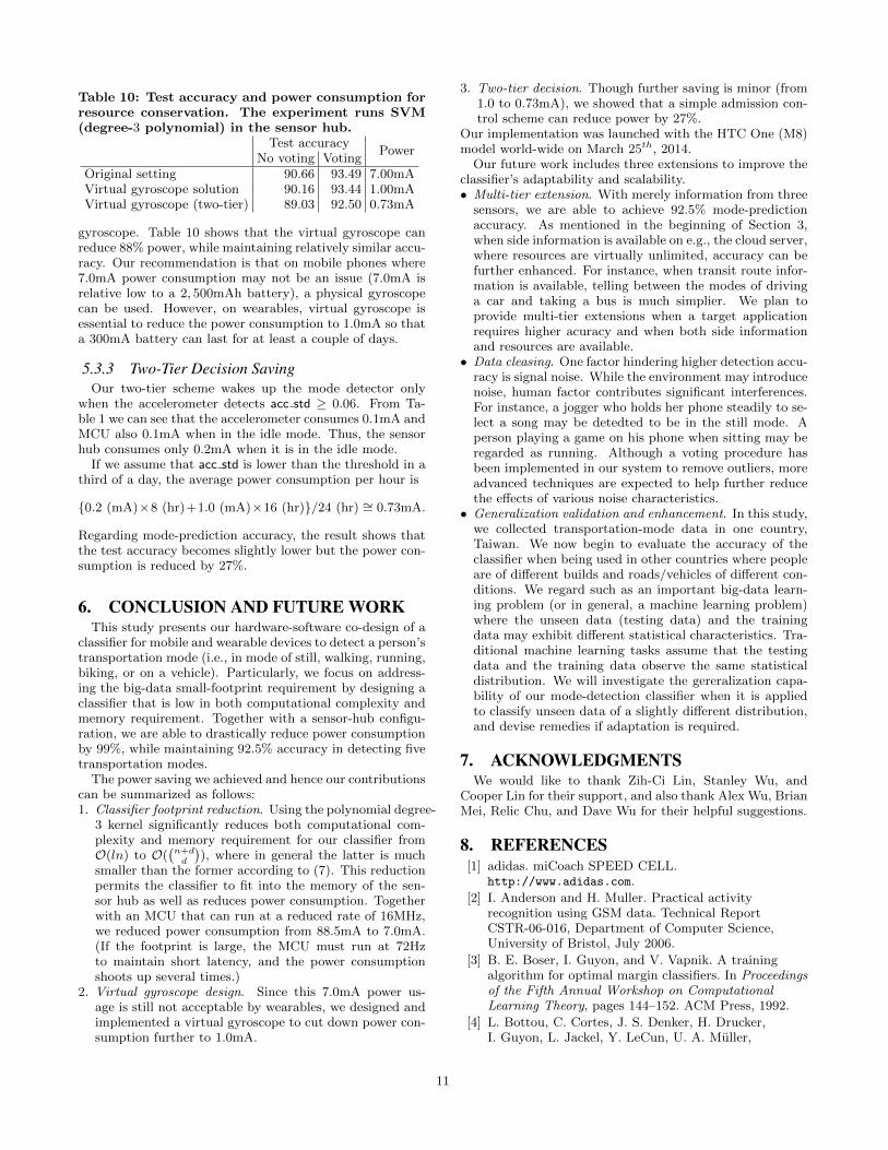
Table 10: Test accuracy and power consumption forresource conservation. The experiment runs SVM(degree-3 polynomial) in the sensor hub.

Test accuracyPower

No voting VotingOriginal setting 90.66 93.49 7.00mAVirtual gyroscope solution 90.16 93.44 1.00mAVirtual gyroscope (two-tier) 89.03 92.50 0.73mA

gyroscope. Table 10 shows that the virtual gyroscope canreduce 88% power, while maintaining relatively similar accu-racy. Our recommendation is that on mobile phones where7.0mA power consumption may not be an issue (7.0mA isrelative low to a 2, 500mAh battery), a physical gyroscopecan be used. However, on wearables, virtual gyroscope isessential to reduce the power consumption to 1.0mA so thata 300mA battery can last for at least a couple of days.

5.3.3 Two-Tier Decision SavingOur two-tier scheme wakes up the mode detector only

when the accelerometer detects acc std ≥ 0.06. From Ta-ble 1 we can see that the accelerometer consumes 0.1mA andMCU also 0.1mA when in the idle mode. Thus, the sensorhub consumes only 0.2mA when it is in the idle mode.

If we assume that acc std is lower than the threshold in athird of a day, the average power consumption per hour is

{0.2 (mA)×8 (hr)+1.0 (mA)×16 (hr)}/24 (hr) ∼= 0.73mA.

Regarding mode-prediction accuracy, the result shows thatthe test accuracy becomes slightly lower but the power con-sumption is reduced by 27%.

6. CONCLUSION AND FUTURE WORKThis study presents our hardware-software co-design of a

classifier for mobile and wearable devices to detect a person’stransportation mode (i.e., in mode of still, walking, running,biking, or on a vehicle). Particularly, we focus on address-ing the big-data small-footprint requirement by designing aclassifier that is low in both computational complexity andmemory requirement. Together with a sensor-hub configu-ration, we are able to drastically reduce power consumptionby 99%, while maintaining 92.5% accuracy in detecting fivetransportation modes.

The power saving we achieved and hence our contributionscan be summarized as follows:1. Classifier footprint reduction. Using the polynomial degree-

3 kernel significantly reduces both computational com-plexity and memory requirement for our classifier fromO(ln) to O(

(n+dd

)), where in general the latter is much

smaller than the former according to (7). This reductionpermits the classifier to fit into the memory of the sen-sor hub as well as reduces power consumption. Togetherwith an MCU that can run at a reduced rate of 16MHz,we reduced power consumption from 88.5mA to 7.0mA.(If the footprint is large, the MCU must run at 72Hzto maintain short latency, and the power consumptionshoots up several times.)

2. Virtual gyroscope design. Since this 7.0mA power us-age is still not acceptable by wearables, we designed andimplemented a virtual gyroscope to cut down power con-sumption further to 1.0mA.

3. Two-tier decision. Though further saving is minor (from1.0 to 0.73mA), we showed that a simple admission con-trol scheme can reduce power by 27%.

Our implementation was launched with the HTC One (M8)model world-wide on March 25th, 2014.

Our future work includes three extensions to improve theclassifier’s adaptability and scalability.• Multi-tier extension. With merely information from three

sensors, we are able to achieve 92.5% mode-predictionaccuracy. As mentioned in the beginning of Section 3,when side information is available on e.g., the cloud server,where resources are virtually unlimited, accuracy can befurther enhanced. For instance, when transit route infor-mation is available, telling between the modes of drivinga car and taking a bus is much simplier. We plan toprovide multi-tier extensions when a target applicationrequires higher acuracy and when both side informationand resources are available.• Data cleasing. One factor hindering higher detection accu-

racy is signal noise. While the environment may introducenoise, human factor contributes significant interferences.For instance, a jogger who holds her phone steadily to se-lect a song may be detedted to be in the still mode. Aperson playing a game on his phone when sitting may beregarded as running. Although a voting procedure hasbeen implemented in our system to remove outliers, moreadvanced techniques are expected to help further reducethe effects of various noise characteristics.• Generalization validation and enhancement. In this study,

we collected transportation-mode data in one country,Taiwan. We now begin to evaluate the accuracy of theclassifier when being used in other countries where peopleare of different builds and roads/vehicles of different con-ditions. We regard such as an important big-data learn-ing problem (or in general, a machine learning problem)where the unseen data (testing data) and the trainingdata may exhibit different statistical characteristics. Tra-ditional machine learning tasks assume that the testingdata and the training data observe the same statisticaldistribution. We will investigate the gereralization capa-bility of our mode-detection classifier when it is appliedto classify unseen data of a slightly different distribution,and devise remedies if adaptation is required.

7. ACKNOWLEDGMENTSWe would like to thank Zih-Ci Lin, Stanley Wu, and

Cooper Lin for their support, and also thank Alex Wu, BrianMei, Relic Chu, and Dave Wu for their helpful suggestions.

8. REFERENCES[1] adidas. miCoach SPEED CELL.

http://www.adidas.com.

[2] I. Anderson and H. Muller. Practical activityrecognition using GSM data. Technical ReportCSTR-06-016, Department of Computer Science,University of Bristol, July 2006.

[3] B. E. Boser, I. Guyon, and V. Vapnik. A trainingalgorithm for optimal margin classifiers. In Proceedingsof the Fifth Annual Workshop on ComputationalLearning Theory, pages 144–152. ACM Press, 1992.

[4] L. Bottou, C. Cortes, J. S. Denker, H. Drucker,I. Guyon, L. Jackel, Y. LeCun, U. A. Muller,

11

E. Sackinger, P. Simard, and V. Vapnik. Comparisonof classifier methods: a case study in handwritingdigit recognition. In International Conference onPattern Recognition, pages 77–87, 1994.

[5] C.-C. Chang and C.-J. Lin. LIBSVM: A library forsupport vector machines. ACM Transactions onIntelligent Systems and Technology, 2:27:1–27:27,2011. Software available athttp://www.csie.ntu.edu.tw/~cjlin/libsvm.

[6] E. Y. Chang. Foundations of Large-Scale MultimediaInformation Management and Retrieval.Springer-Verlag New York Inc, New York, 2011.

[7] Y.-W. Chang, C.-J. Hsieh, K.-W. Chang,M. Ringgaard, and C.-J. Lin. Training and testinglow-degree polynomial data mappings via linear SVM.Journal of Machine Learning Research, 11:1471–1490,2010.

[8] C. Cortes and V. Vapnik. Support-vector network.Machine Learning, 20:273–297, 1995.

[9] Fitbit. Flex wristband. http://www.fitbit.com.

[10] Y. Freund and R. E. Schapire. A decision-theoreticgeneralization of on-line learning and an application toboosting. Journal of Computer and System Sciences,55(1):119–139, 1997.

[11] M. Garofalakis, D. Hyun, R. Rastogi, and K. Shim.Building decision trees with constraints. Data Miningand Knowledge Discovery, 7(2):187–214, 2003.

[12] K.-S. Goh, E. Chang, and K.-T. Cheng. Svm binaryclassifier ensembles for image classification. InProceedings of the Tenth International Conference onInformation and Knowledge Management (CIKM),pages 395–402, 2001.

[13] Google. Google now.http://www.google.com/landing/now/.

[14] M. Hall, E. Frank, G. Holmes, B. Pfahringer,P. Reutemann, and I. H. Witten. The WEKA datamining software: An update. SIGKDD Explorations,11, 2009.

[15] HTC. HTC Research. http://research.htc.com/2014/06/publication14001/.

[16] S. Knerr, L. Personnaz, and G. Dreyfus. Single-layerlearning revisited: a stepwise procedure for buildingand training a neural network. In Neurocomputing:Algorithms, Architectures and Applications, 1990.

[17] J. Lester, T. Choudhury, and G. Borriello. A practicalapproach to recognizing physical activities. In LectureNotes in Computer Science, volume 3096. Springer,2006.

[18] H. Lu, J. Yang, Z. Liu, N. D. Lane, T. Choudhury,and A. T. Campbell. The jigsaw continuous sensingengine for mobile phone applications. In Proceedingsof the 8th ACM Conference on Embedded NetworkedSensor Systems (SenSys), pages 71–84, 2010.

[19] Monsoon Solution Inc. Power monitor.http://www.msoon.com/.

[20] M. Y. Mun, D. Estrin, J. Burke, and M. Hansen.Parsimonious mobility classification using GSM andWiFi traces. In Proceedings of the Fifth Workshop onEmbedded Networked Sensors (HotEmNets), 2008.

[21] S. Nath. ACE: exploiting correlation forenergy-efficient and continuous context sensing. InProceedings of the 10th International Conference on

Mobile Systems, Applications, and Services (MobiSys),pages 29–42, 2012.

[22] Nike. Fuelband. http://www.nike.com/us/en_us/c/nikeplus-fuelband.

[23] J. R. Quinlan. C4.5: Programs for Machine Learning.Morgan Kaufmann, 1993.

[24] K. K. Rachuri, C. Mascolo, M. Musolesi, and P. J.Rentfrow. SociableSense: exploring the trade-offs ofadaptive sampling and computation offloading forsocial sensing. In Proceedings of the 17th AnnualInternational Conference on Mobile Computing andNetworking, pages 73–84, 2011.

[25] S. Reddy, M. Mun, J. Burke, D. Estrin, M. Hansen,and M. Srivastava. Using mobile phones to determinetransportation modes. ACM Transactions on SensorNetworks, 6(2):13:1–13:27, 2010.

[26] T. Sohn, A. Varshavsky, A. LaMarca, M. Y. Chen,T. Choudhury, I. Smith, S. Consolvo, andW. Griswold. Mobility detection using everyday GSMtraces. In Proceedings of the 8th InternationalConference on Ubiquitous Computing, 2006.

[27] D. Specifications. Sony smartwatch 2-battery.http://www.devicespecifications.com/en/

model-battery/518829ce.

[28] V. Srinivasan and T. Phan. An accurate two-tierclassifier for efficient duty-cycling of smartphoneactivity recognition systems. In Proceedings of theThird International Workshop on Sensing Applicationson Mobile Phones (PhoneSense), pages 11:1–11:5,2012.

[29] M. E. Stanley. Building a virtual gyro.https://community.freescale.com/community/

the-embedded-beat/blog/2013/03/12/

building-a-virtual-gyro, 2013.

[30] L. Stenneth, O. Wolfson, P. S. Yu, and B. Xu.Transportation mode detection using mobile phonesand GIS information. In Proceedings of the 19th ACMSIGSPATIAL International Conference on Advancesin Geographic Information Systems, GIS ’11, 2011.

[31] S. Wang, C. Chen, and J. Ma. Accelerometer basedtransportation mode recognition on mobile phones. InProceedings of the 2010 Asia-Pacific Conference onWearable Computing Systems, pages 44–46, 2010.

[32] P. Widhalm, P. Nitsche, and N. Brandie. Transportmode detection with realistic smartphone sensor data.In Proceedings of the 21st International Conference onPattern Recognition (ICPR), pages 573–576, 2012.

[33] G. Wu and E. Y. Chang. KBA: kernel boundaryalignment considering imbalanced data distribution.IEEE Transactions on Knowledge and DataEngineering, 17(6):786–795, 2005.

[34] J. Yang. Toward physical activity diary: motionrecognition using simple acceleration features withmobile phones. In Proceedings of the 1st internationalworkshop on Interactive multimedia for consumerelectronics, pages 1–10, 2009.

[35] Y. Zheng, Q. Li, Y. Chen, X. Xie, and W.-Y. Ma.Understanding mobility based on gps data. InProceedings of the 10th International Conference onUbiquitous Computing (UbiComp), pages 312–321,New York, NY, USA, 2008. ACM.

12