Bicriteria train scheduling for high-speed passenger railroad planning applications

Bicriteria train scheduling for high-speed passenger railroad planning applications Submitted to feature issue on scheduling with multiple objectives, European Journal of Operational Research Xuesong Zhou a,*, Ming Zhong b

a Department of Civil & Environmental Engineering and Maryland Transportation Initiative, University of Maryland, College Park, MD 20742, USA b Robert H. Smith School of Business, University of Maryland, College Park, MD 20742, USA *Corresponding author. Tel: +1-301-405-1778; fax:+1-301-405-2585. Email address: [email protected] (X. Zhou) First version: January, 2003 Revised 23 September 2003 Revised 22 February 2004

2

Bicriteria train scheduling for high-speed passenger railroad planning applications Xuesong Zhou a,*, Ming Zhong b a Department of Civil & Environmental Engineering and Maryland Transportation Initiative, University of Maryland, College Park, MD 20742, USA b Robert H. Smith School of Business, University of Maryland, College Park, MD 20742, USA *Corresponding author. Tel: +1-301-405-1778; fax:+1-301-405-2585. Email address: [email protected] (X. Zhou) Abstract

This paper is concerned with a double-track train scheduling problem for planning applications with multiple objectives. Focusing on a high-speed passenger rail line in an existing network, the problem is to minimize both (1) the expected waiting times for high-speed trains and (2) the total travel times of high-speed and medium-speed trains. By applying two practical priority rules, the problem with second criterion is decomposed and formulated as a series of multi-mode resource constrained project scheduling problems in order to explicitly model acceleration and deceleration times. A branch-and-bound algorithm with effective dominance rules is developed to generate Pareto solutions for the bicriteria scheduling problem, and a beam search algorithm with utility evaluation rules is used to construct a representative set of non-dominated solutions. A case study based on Beijing-Shanghai high-speed railroad in China illustrates the methodology and compares the performance of the proposed algorithms. Keywords: Scheduling; Multiple objective programming; Transportation; Railway

3

1. Introduction

Being an efficient and economic public transportation mode, rail plays an important role in the passenger and freight transportation markets, especially in European and Asian countries. The level-of-service of train timetables is a key factor in travelers’ and carriers’ decision for selecting desirable services. In addition, train timetables are the basis for performing locomotive and crew scheduling, and their quality further affects the investments and operating costs on cars, engines, crew and fuel costs. In response to increasing competition with other transportation modes, such as auto, truck and air, optimizing train schedules becomes an essential approach for railroad industries to increase revenues and reduce the operation costs.

More formally, the train scheduling problem is to find an optimal train timetable (or referred to as train working diagram), subject to a number of operational and safety requirements, such as overtaking and crossing headway constraints. Depending on application areas, practical train scheduling problems have different objectives. Specifically, planning applications are concerned with how to generate train schedules so as to satisfy passenger and freight traffic demand and minimize the overall operational costs, while real-time applications aim to adjust the daily and hourly train operation schedules so as to improve on-time performance and reliability.

In planning applications, the train scheduling activities are typically conducted in two phases: (1) line planning (i.e. sketch planning), which is to determine the routes, frequencies, and stop schedules of trains, and (2) schedule generation (i.e. detailed scheduling), which is to construct the arrival and departure times for each train at passing stations. With respect to the line planning problem, Assad (1980) provided an excellent review on the previous studies in the 1970s. Recently, Bussieck et al. (1997) gave an integer programming formulation for line planning on a railroad network, and Chang et al. (2000) proposed a multi-objective linear programming model for determining both stop and frequency schedules. The research for the detailed train scheduling starts from Szpigel’s work (1973) with the objective of minimizing the total travel time, motivated by Greenberg’s branch-and-bound approach (1968) for the job-shop scheduling problem. Significant progress has been made on exact solution algorithms in the last decade, for example, to mention a few, the operational train scheduling problem that minimizes the deviation from the planned schedules (Kraay and Harker, 1995), lower bound estimation methods for the branch-and-bound solution algorithm (Higgins et al., 1996) and Lagrangian relaxation techniques (Brannlund et al., 1998). Two aspects regarding real-time applications are widely discussed in the literature, namely efficient heuristic methods (e.g. Adenso-Diaz et al., 1999; Sahin, 1999; Zhou, et al., 1998) and train schedule reliability (e.g. Kraay and Harker, 1995; Higgins and Kozan, 1998; Kraft, 1998). Several works have addressed the train scheduling problem with multi-criteria (e.g. Higgins and Kozan, 1998; Ma et al., 2002). The additional objectives in these studies mainly focus on the supply side, such as fuel costs for locomotives, labor costs for crews, and such objectives are typically simplified to be a weighted linear combination. However, a decision maker’s preference information regarding the weights is typically difficult to obtain a priori, and the decision maker tends to identify the most-preferred solution based on the generated efficient solution set. Cordeau et al. (1998) gave a comprehensive survey for the train scheduling problem and its inherent connection to other railroad routing and scheduling problems.

While most existing studies concentrate on real-time applications, schedule generation for planning applications has not received adequate attention, especially timetabling for inter-city passenger services. According to studies on the transportation demand analysis (e.g. KPMG Peat Marwick and Koppelman, 1990; Bhat, 1995), four alternative-specific attributes mainly affect the inter-city mode choice behavior: travel cost, frequency, in-vehicle time and out-of-vehicle time. In the rail mode, train timetables determine the last three elements. Particularly, the in-vehicle time is the total time traveling on trains, and the out-of-vehicle time includes the waiting time for a passenger to board the train or to transfer. In order to improve market share, railway industries should shift their focus from traditional operation-constrained decision making to market-driven decision making, which highlights the passenger demand side.

This paper considers the train schedule generation problem on a double-track corridor, specifically, the timetable planning application on Beijing-Shanghai high-speed passenger railroad. As the busiest railroad corridor in China, the current rail system covers the area that produces almost 40% of the total industry and agriculture in this country and it is running at or near capacity. Two types of trains, namely high-speed trains (250-300 km/h) and medium-speed trains (160 km/h), are designed to operate in the same track system. In order to serve the large volume of traffic passing through this corridor, medium-speed trains are planned to run on both high-speed line and adjacent regular rail lines so as to reduce connecting delay for

4

interline travel. On the other hand, high-speed trains provide direct service for inter-city travel in this area. Wong et al. (2002) addressed the management/ownership issues, and Nie et al. (2000) proposed simulation-based models for traffic organization. In fact, the above mixed operation policy with two types of passenger trains also calls for more sophisticated timetable planning methodology and techniques to precisely synchronize high-speed and medium-speed train movements.

First, as a fast transit mode, the high-speed train service is expected to provide a “perfect” schedule with high frequency and even departure time intervals. On the other hand, if a possible conflict exists, the medium-speed trains have to yield to high-speed trains that always hold higher priority. Consequently, the traditional sequential planning approach (scheduling high-speed first and medium-speed trains next) will result in extremely long travel times for medium-speed train passengers, and fail to balance service quality for both types of trains. In this case, the decision maker would like to obtain non-dominated solutions, i.e. Pareto optima, so as to retrieve the corresponding trade-offs and make appropriate decisions.

In addition, even with highly efficient acceleration and deceleration performance, high-speed trains still take at least several minutes to fully stop or reach the cruise speed, due to the safety and passenger comfort requirements. In this situation, the related timetabling procedure has to exactly take into account the time required for acceleration and deceleration. To the authors’ knowledge, most existing studies for the schedule generation problem do not explicitly model acceleration and deceleration times, which might be due to the different operation polices in different countries. Kraft (1987) proposed a branch-and-bound procedure to enumerate the possible meeting instructions with acceleration penalties in a single-track rail line. Several researchers in China (e.g. Zhou et al., 1998; Ma et al., 2002) used simulation-based heuristic methods to consider the acceleration and deceleration characteristics.

In order to satisfy the above requirements in real-world applications, this paper considers the above train scheduling problem as a multi-mode flow-shop scheduling problem with multiple criteria. Specifically, a double-track rail corridor consists of a set of sections (machines) and a set of trains (jobs). Each train has a predefined route (processing order) through sections, and we can view a train traveling along a route as a procedure of completing a series of activities with respect to sections. To model acceleration and deceleration time losses, an activity is assumed to have multiple execution modes, corresponding to different running states (i.e. stop or no-stop) and durations. Regarding multi-mode resource constrained project scheduling, Patterson et al. (1989, 1990) first proposed a branch-and-bound solution algorithm, and Sprecher and Drexl (1998) improved the algorithm performance by adopting effective dominance rules. Brucker et al. (1999) provided a complete treatment on the resource-constrained project scheduling problem for single-mode and multi-mode cases, and illustrated its connection with the machine scheduling problem.

Extensive research has been done on single machine scheduling with multiple objectives (Nagar et al. 1995), but limited studies have been conducted on the multi-machine case. Along the implicit enumeration approach, which includes branch-and-bound and dynamic programming methods, Sayin and Karabati (1999) addressed the two-machine flow-shop scheduling problem with simultaneous bicriteria, and T’kindt et al. (2003) discussed a similar setting with lexicographical bicriteria. Meanwhile, several meta-heuristics methods, such as Genetic Algorithm and Tabu Search are also proposed to deal with large-size applications within reasonable computation time (e.g. Neppalli et al., 1996; T'kindt et al., 2002; Framinan et al. 2002). Most of the above studies employ the common criteria in the machine schedule context, namely minimizing makespan and minimizing total completion time. A recent review on this topic has been presented by T’kindt and Billaut (2001).

The organization of this paper is as follows. First, we present an integer programming formulation for the double-track train scheduling problem. To solve the timetabling problem with acceleration and deceleration time constraints, Section 3 discusses a problem decomposition strategy and provides an implicit enumeration algorithm for the subproblem. In Section 4, a branch-and-bound algorithm with effective dominance rules is developed to generate Pareto solutions for the bicriteria scheduling problem, and a beam search algorithm with utility evaluation rules is used to construct a representative set of non-dominated solutions. Finally, the proposed algorithms are evaluated based on the planning application for Beijing-Shanghai high-speed passenger railroad. 2. The integer programming formulation

5

The following notation is used to formulate the double-track train scheduling problem with acceleration and deceleration consideration. All the parameters and variables are nonnegative integers, and the unit of time is one minute. Table 1. Subscripts and parameters Symbol Definition Nh the total number of high-speed trains. N the total number of high-speed and medium-speed trains. K the total number of sections in the railroad line to be considered. i subscript of trains (jobs) , i = 1, 2, …, N. k subscript of sections (machines), k = 1, 2, …, K. Ih the set of high-speed trains, i.e. i=1, 2, …, Nh and |Ih|=Nh. Im the set of medium-speed trains, i.e. i= Nh+1, Nh+2, …, N and |Im|=N-Nh. I the set of trains, i.e. i=1, 2, …, N and I=Ih ∪Im and |I|=N. V the set of sections, i.e. |V|=K. u subscript of train type , u =1 for a high-speed train, u =2 for a medium-speed train. qi train type for train i, i.e. qi =1 for hIi ∈ , and qi =2 for mIi ∈ .

kup , pure running time for train type u at section k without acceleration and deceleration times.

kua

,τ time required for acceleration at the upstream station of section k with respect to train type u.

kud

,τ time required for deceleration at the downstream station of section k with respect to train type u.

kvueh ,, minimum headway between train types u and v entering section k.

kvulh ,, minimum headway between train types u and v leaving section k.

kis , scheduled minimum stop time for train i at station k, i.e. minimum stop time before train i entering section k.

id~

preferred departure time for train i at its origin, i.e. the preferred release time for job i.

ig maximum deviation for departure time of train i from its preferred departure time. ( ig = 0

mIi ∈∀ ). M a large positive number. Table 2. Decision variables Symbol Definition

id departure time for train i at its origin.

iy interdeparture time between train i and train i+1.

ekix , entering time for train i to section k, i.e. the starting time for job i on machine k.

lkix , leaving time for train i from section k, i.e. the ending time for job i on machine k.

akit , actual acceleration time for train i at the upstream station of section k. i.e. at station k.

dkit , actual deceleration time for train i at the downstream station of section k .i.e. at station k + 1.

iC total travel time for train i.

kjiB ,, 0 or 1, indicating if train i enters section k earlier or later than train j, respectively.

akiB , 0 or 1, indicating if train i bypasses/stops at the upstream station of section k, respectively.

6

dkiB , 0 or 1, indicating if train i bypasses/stops at the downstream station of section k, respectively.

The constraints used in the double-track scheduling model are presented as the following.

Allowable adjustment for departure time: (2N constraints)

Iigddgd iiiii ∈∀+≤≤− ~~ (1)

Interdeparture time: (Nh -1 constraints for high-speed trains)

1 \ i i i h hy d d i I N+= − ∀ ∈ (2) Departure time: (N constraints)

Iidx iei ∈∀=1, (3)

Total travel time: (N constraints) IixxC e

il

Kii ∈∀−= 1,, (4)

Dwell time: (N×(K-1) constraints) 1\,,1,, =∈∀∈∀≥− − kVkIisxx ki

lki

eki (5)

Travel time on sections: (N×K constraints) VkIittpxx d

kiakikiq

eki

lki ∈∀∈∀++=− ,,,),(,, (6)

Acceleration time: (2×N×K constraints) 1,1\, 1,1,,, ==∈∀∈∀−≥× −

ai

lki

eki

aki BkVkIixxMB (7)

VkIiBt kiqaa

kiaki ∈∀∈∀×= ,),(,, τ (8)

Deceleration time: (2×N×K constraints) 1,\, ,,1,, ==∈∀∈∀−≥× +

dKi

lki

eki

dki BKkVkIixxMB (9)

VkIiBt kiqdd

kidki ∈∀∈∀×= ,),(,, τ (10)

Minimum headway: (N× (N-1) ×K× 4 constraints) VkIjijihxxorhxxeither kjqiq

eeki

ekjkiqjq

eekj

eki ∈∀∈≠∀≥−≥− ,,,),(),(,,),(),(,, (11)

VkIjijihxxorhxxeither kjqiqll

kil

kjkiqjqll

kjl

ki ∈∀∈≠∀≥−≥− ,,,),(),(,,),(),(,, (12)

To model the above “either-or” type constraints, we have

VkIjijiMBhxx kjiiqjqee

kje

ki ∈∀∈≠∀×−−≥− ,,,)1( ,,)(),(,, (13)

VkIjijiMBhxx kjijqiqee

kie

kj ∈∀∈≠∀×−≥− ,,,,,)(),(,, (14)

VkIjijiMBhxx kjiiqjqll

kjl

ki ∈∀∈≠∀×−−≥− ,,,)1( ,,)(),(,, (15)

VkIjijiMBhxx kjijqiqll

kil

kj ∈∀∈≠∀×−≥− ,,,,,)(),(,, . (16)

Without loss of generality, we only consider the outbound trains in the double-track rail line, which

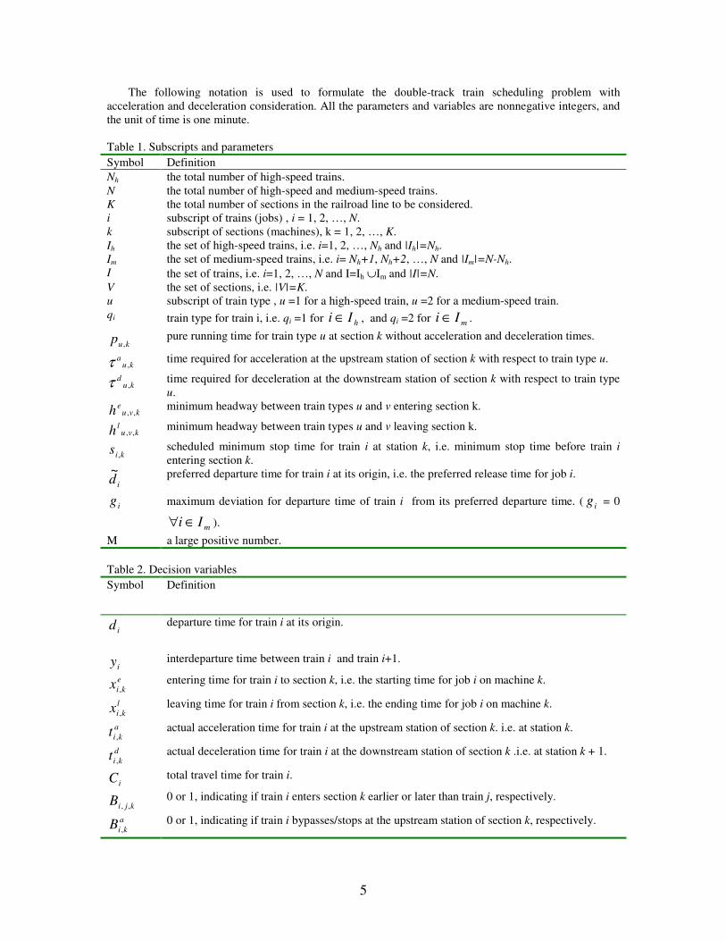
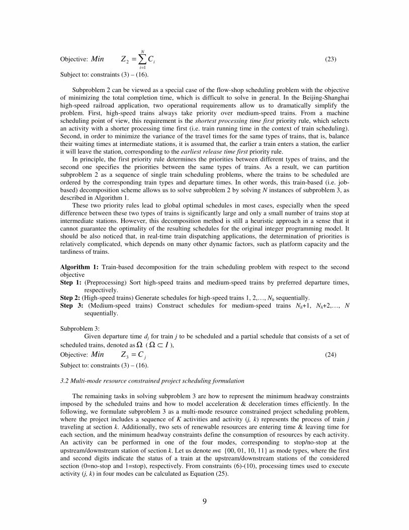
pass sections 1, 2, …, K-1, K. For each train type, the corresponding pure running time, acceleration time and deceleration time at each section are calibrated from train performance calculation. The minimum stop times and preferred departure times are determined in the previous line planning stage. In particular, the preferred departure times for high-speed trains are assumed to give even departure time intervals subject to the scheduled frequency. In this study, the preferred departure times for medium-speed trains are set to be the existing transfer times from outside lines to the high-speed rail line, and no adjustment is allowed for simplicity. Figure 1 illustrates the related parameters and variables, in which high-speed train i overtakes medium-speed train j at station k.

7

section k

section k-2

xlj,k

xej,k

section k-1

di section 1

hlq(j),q(i),k-1

Time axis

ii gd −~ii gd +~

id~

station k+1

station 1

station k-2

station k-1

station kxl

j,k-1

dj

......

heq(i),q(j),k

Figure 1 Illustration for a double-track train schedule Constraint (1) implies that a certain amount of adjustments are allowed for high-speed trains with

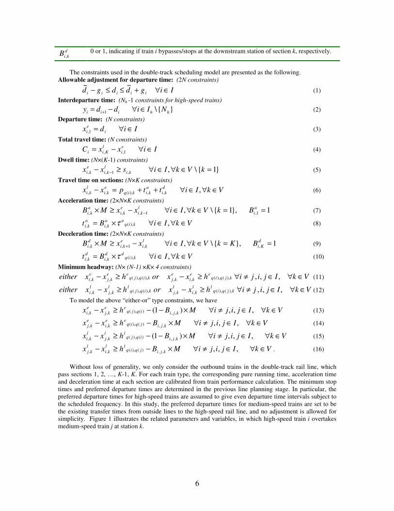
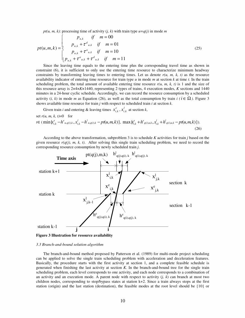
respect to the preferred departure times. Interdeparture constraint (2) will be used in calculating the expected passenger waiting time in the first objective function described later. Constraint (3) relates the actual departure time to the entering time of a train at the first section, and similarly constraint (4) links the travel time to the leaving time of a train at the last section. As shown in constraint (5), the actual dwell time should be no less than the planed minimum stop time, more precisely, the actual dwell time equals to minimum stop time plus yield time. An important feature in this model is that it considers acceleration and deceleration times, represented by constraints (6) to (10). Figure 2 shows that if train i stops at station k,

then the actual stop time lki

eki xx 1,, −− is greater than 0, and the required times for acceleration and

deceleration at station k have to be set to kiqa

),(τ or 1),( −kiqdτ . From the resource-constrained project

scheduling point of view, time is the discrete resource in this problem, and there are four execution modes for train i traveling at section k, namely (1) bypasses stations k and k+1, (2) bypasses station k but stops at station k+1, (3) stops at station k but bypasses station k+1 and (4) stops at both stations k and k+1. The headway constraints (11) to (16) describe the minimum headway requirements between the departure times and arrival times of consecutive trains at the same station.

section k

Time axis

station k-1

station k

station k+1

section k-1

pq(i), k-1 pq(i), k-1 1),( −kiqdτ

pq(i), kkiq

a),(τ pq(i), k

bypass station k stop at station k Figure 2 Illustration for acceleration time and deceleration time

8

The first objective of this problem is to minimize the variation of interdeparture times for high-speed trains, i.e.,

−

=

−−

==1

1

21 )(

21

)(hN

iii

h

yyN

YVarZMin , (17)

and the second objective is to minimize the total travel time, i.e.,

=

=N

iiCZMin

12 , (18)

Irregular departure times create significant variation in passenger occupancy rates, and further lead to the loss of efficiency in utilizing platforms and locomotives. More importantly, if assuming passengers independently and randomly arrive at the terminal, we can show that the first criterion is identical to minimizing the expected out-of-train waiting time, that is, the waiting time from a passenger arriving at the terminal to the departure time of the next train. Let Y be the random variable of interdeparture time for high-speed trains, and let W be the random variable of out-of-train waiting time. The probability density function of Y can be calculated from the frequency of yi, i =1, 2, …, Nh -1. The random incidence theorem described by Larson and Odoni (1981) provides an excellent mathematical formula to quantify the expected waiting time E(W) based on the distribution of interdeparture time Y in transportation service systems, i.e.,

2)(

)(2)(

)(2)()(

)(2 YE

YEYVar

YEYEYVar

WE +=+= . (19)

In an ideal schedule with even interdeparture times, Var(Y) =0, so expected waiting time E(W) reaches

the minimum of 2

)(YE. If assuming departure events follow a Poisson process, then Var(Y)=E(Y)2 and

E(W)=E(Y). Note that, E(Y) (i.e. iy ) here is determined by the number of high-speed trains in the planning horizon, so it is a constant in Equation (19). Thus, E(W) is linearly proportional to Var(Y), and the first objective is equivalent to minimizing the expected waiting time for high-speed train passengers at origin stations. As the second criterion is equivalent to minimizing the total in-vehicle time, both objectives in this study can be interpreted as time attributes related to the service qualities of train timetables. 3. Train scheduling problems with single objective 3.1 Train-based decomposition

Since the problem with the first objective (17) only involves variables yi and di, which are restricted by constraints (1) and (2), this problem can be reduced to subproblem 1, corresponding to a combinatorial optimization model for determining departure times for high-speed trains. Obviously, the optimal solution can be obtained by evenly distributing departure times for high-speed trains, that is, ii yy = for i =1, 2, …, Nh -1 and Z1=0. On the other hand, if assuming departure times di’s are given for both high-speed and medium-speed trains, the model with the second objective (18) is equivalent to a regular double-track train schedule generation problem. Subproblem 1:

Objective: −

=

−−

==1

1

21 )(

21

)(hN

iii

h

yyN

YVarZMin (20)

Subject to: hiiiii Iigddgd ∈∀+≤≤− ~~ (21)

1 \i i i h hy d d i I i N+= − ∀ ∈ = . (22)

Subproblem 2: Given departure times di for Ii ∈ ,

9

Objective: =

=N

iiCZMin

12 (23)

Subject to: constraints (3) – (16).

Subproblem 2 can be viewed as a special case of the flow-shop scheduling problem with the objective of minimizing the total completion time, which is difficult to solve in general. In the Beijing-Shanghai high-speed railroad application, two operational requirements allow us to dramatically simplify the problem. First, high-speed trains always take priority over medium-speed trains. From a machine scheduling point of view, this requirement is the shortest processing time first priority rule, which selects an activity with a shorter processing time first (i.e. train running time in the context of train scheduling). Second, in order to minimize the variance of the travel times for the same types of trains, that is, balance their waiting times at intermediate stations, it is assumed that, the earlier a train enters a station, the earlier it will leave the station, corresponding to the earliest release time first priority rule.

In principle, the first priority rule determines the priorities between different types of trains, and the second one specifies the priorities between the same types of trains. As a result, we can partition subproblem 2 as a sequence of single train scheduling problems, where the trains to be scheduled are ordered by the corresponding train types and departure times. In other words, this train-based (i.e. job-based) decomposition scheme allows us to solve subproblem 2 by solving N instances of subproblem 3, as described in Algorithm 1.

These two priority rules lead to global optimal schedules in most cases, especially when the speed difference between these two types of trains is significantly large and only a small number of trains stop at intermediate stations. However, this decomposition method is still a heuristic approach in a sense that it cannot guarantee the optimality of the resulting schedules for the original integer programming model. It should be also noticed that, in real-time train dispatching applications, the determination of priorities is relatively complicated, which depends on many other dynamic factors, such as platform capacity and the tardiness of trains. Algorithm 1: Train-based decomposition for the train scheduling problem with respect to the second objective Step 1: (Preprocessing) Sort high-speed trains and medium-speed trains by preferred departure times,

respectively. Step 2: (High-speed trains) Generate schedules for high-speed trains 1, 2,…, Nh sequentially. Step 3: (Medium-speed trains) Construct schedules for medium-speed trains Nh+1, Nh+2,…, N

sequentially. Subproblem 3:

Given departure time dj for train j to be scheduled and a partial schedule that consists of a set of scheduled trains, denoted as Ω ( I⊂Ω ), Objective: jCZMin =3 (24)

Subject to: constraints (3) – (16). 3.2 Multi-mode resource constrained project scheduling formulation

The remaining tasks in solving subproblem 3 are how to represent the minimum headway constraints

imposed by the scheduled trains and how to model acceleration & deceleration times efficiently. In the following, we formulate subproblem 3 as a multi-mode resource constrained project scheduling problem, where the project includes a sequence of K activities and activity (j, k) represents the process of train j traveling at section k. Additionally, two sets of renewable resources are entering time & leaving time for each section, and the minimum headway constraints define the consumption of resources by each activity. An activity can be performed in one of the four modes, corresponding to stop/no-stop at the upstream/downstream station of section k. Let us denote m∈ 00, 01, 10, 11 as mode types, where the first and second digits indicate the status of a train at the upstream/downstream stations of the considered section (0=no-stop and 1=stop), respectively. From constraints (6)-(10), processing times used to execute activity (j, k) in four modes can be calculated as Equation (25).

10

pt(u, m, k): processing time of activity (j, k) with train type u=q(j) in mode m

=++=+=+

=

=

111001

00

),,(

,,,

,,

,,

,

mifp

mifp

mifp

mifp

kmupt

kud

kua

ku

kua

ku

kud

ku

ku

ττττ

(25)

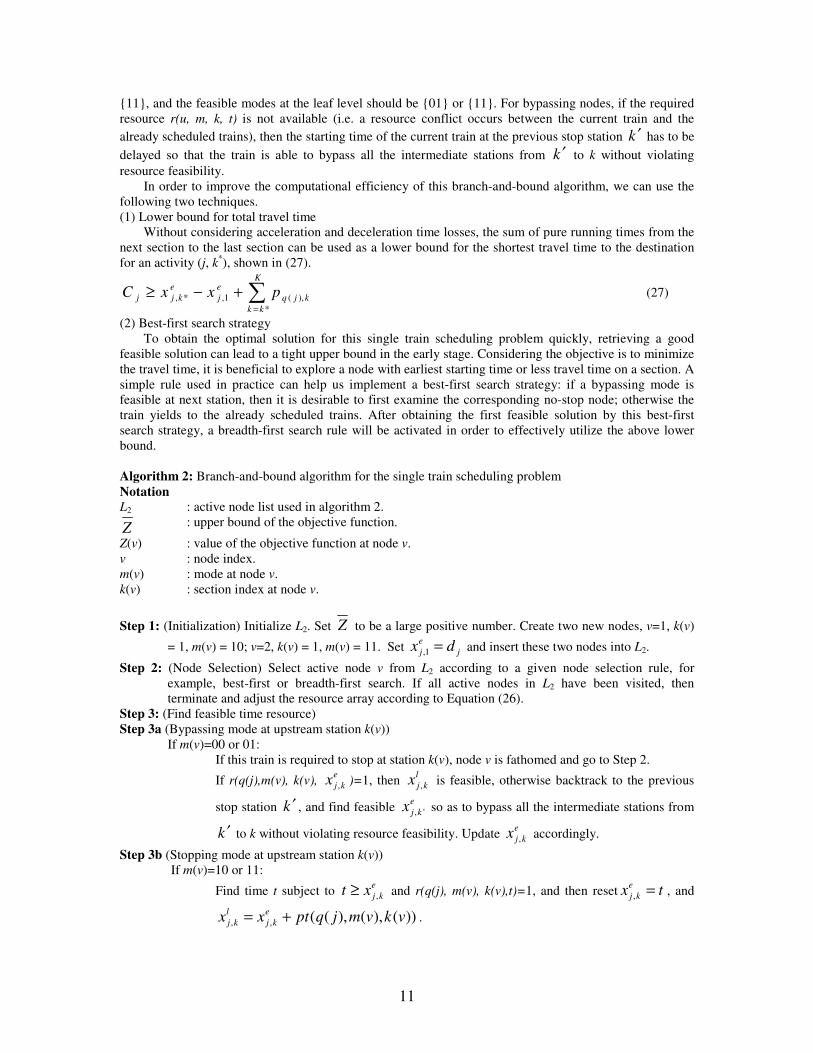
Since the leaving time equals to the entering time plus the corresponding travel time as shown in constraint (6), it is sufficient to only use the entering time resource to characterize minimum headway constraints by transforming leaving times to entering times. Let us denote r(u, m, k, t) as the resource availability indicator of entering time resource for train type u in mode m at section k at time t. In the train scheduling problem, the total amount of available entering time resource r(u, m, k, t) is 1 and the size of this resource array is 2×4×K×1440, representing 2 types of trains, 4 execution modes, K sections and 1440 minutes in a 24-hour cyclic schedule. Accordingly, we can record the resource consumption by a scheduled activity (i, k) in mode m as Equation (26), as well as the total consumption by train i ( Ω∈i ). Figure 3 shows available time resource for train j with respect to scheduled train i at section k.

Given train i and entering & leaving times ekix , , l

kix , at section k,

set r(u, m, k, t)=0 for

t∈( ),,(,min ),(,,),(,, kmupthxhx kiqull

kikiquee

ki −−− , ),,(,max ,),(,,),(, kmupthxhx kuiqll

kikuiqee

ki −++ ).

(26) According to the above transformation, subproblem 3 is to schedule K activities for train j based on the

given resource r(q(j), m, k, t). After solving this single train scheduling problem, we need to record the corresponding resource consumption by newly scheduled train j.

section kxl

j,k

xej,k

section k-1

Time axis

station k+1

station k-1

station k

hlq(j),q(i), k

xli,k

pt(q(j),m,k)

j i

heq(j),q(i), k

xei,k

xlj,k-1

hlq(i),q(j), k

heq(i),q(j), k

Figure 3 Illustration for resource availability 3.3 Branch-and-bound solution algorithm

The branch-and-bound method proposed by Patterson et al. (1989) for multi-mode project scheduling

can be applied to solve the single train scheduling problem with acceleration and deceleration features. Basically, the procedure starts with the first activity at section 1, and a complete feasible schedule is generated when finishing the last activity at section K. In the branch-and-bound tree for the single train scheduling problem, each level corresponds to one activity, and each node corresponds to a combination of an activity and an execution mode. A parent node with respect to activity (j, k) can branch at most two children nodes, corresponding to stop/bypass states at station k+2. Since a train always stops at the first station (origin) and the last station (destination), the feasible modes at the root level should be 10 or

11

11, and the feasible modes at the leaf level should be 01 or 11. For bypassing nodes, if the required resource r(u, m, k, t) is not available (i.e. a resource conflict occurs between the current train and the already scheduled trains), then the starting time of the current train at the previous stop station k ′ has to be delayed so that the train is able to bypass all the intermediate stations from k ′ to k without violating resource feasibility.

In order to improve the computational efficiency of this branch-and-bound algorithm, we can use the following two techniques. (1) Lower bound for total travel time

Without considering acceleration and deceleration time losses, the sum of pure running times from the next section to the last section can be used as a lower bound for the shortest travel time to the destination for an activity (j, k*), shown in (27).

=

+−≥K

kkkjq

ej

ekjj pxxC

*),(1,*, (27)

(2) Best-first search strategy To obtain the optimal solution for this single train scheduling problem quickly, retrieving a good

feasible solution can lead to a tight upper bound in the early stage. Considering the objective is to minimize the travel time, it is beneficial to explore a node with earliest starting time or less travel time on a section. A simple rule used in practice can help us implement a best-first search strategy: if a bypassing mode is feasible at next station, then it is desirable to first examine the corresponding no-stop node; otherwise the train yields to the already scheduled trains. After obtaining the first feasible solution by this best-first search strategy, a breadth-first search rule will be activated in order to effectively utilize the above lower bound. Algorithm 2: Branch-and-bound algorithm for the single train scheduling problem Notation L2 : active node list used in algorithm 2.

Z : upper bound of the objective function.

Z(v) : value of the objective function at node v. v : node index. m(v) : mode at node v. k(v) : section index at node v. Step 1: (Initialization) Initialize L2. Set Z to be a large positive number. Create two new nodes, v=1, k(v)

= 1, m(v) = 10; v=2, k(v) = 1, m(v) = 11. Set jej dx =1, and insert these two nodes into L2.

Step 2: (Node Selection) Select active node v from L2 according to a given node selection rule, for example, best-first or breadth-first search. If all active nodes in L2 have been visited, then terminate and adjust the resource array according to Equation (26).

Step 3: (Find feasible time resource) Step 3a (Bypassing mode at upstream station k(v))

If m(v)=00 or 01: If this train is required to stop at station k(v), node v is fathomed and go to Step 2.

If r(q(j),m(v), k(v), ekjx , )=1, then l

kjx , is feasible, otherwise backtrack to the previous

stop station k ′ , and find feasible ekjx ', so as to bypass all the intermediate stations from

k ′ to k without violating resource feasibility. Update ekjx , accordingly.

Step 3b (Stopping mode at upstream station k(v)) If m(v)=10 or 11:

Find time t subject to ekjxt ,≥ and r(q(j), m(v), k(v),t)=1, and then reset txe

kj =, , and

))(),(),((,, vkvmjqptxx ekj

lkj += .

12

Step 4: (Lower bound) Obtain the lower bound of Cj at current node by Inequality (27), if ZC j > , then

fathom node v and go to Step 2.

Step 5: (Upper bound) If k(v)=K, the related schedule is complete. If ZvZ <)( , then update Z by

)(vZZ = and go to Step 2. Step 6: (Generate feasible modes for descendants)

1,,1, ++ += kjl

kje

kj sxx

If this train reaches the last station, If m(v)=00 or 10, create one new node v′: m(v′) = 01, k(v′) = k(v) +1; If m(v)=01 or 11, create one new node v′: m(v′) = 11, k(v′) = k(v) +1;

Else If m(v)=00 or 10, create two new nodes v′ and v′′: m(v′) = 01, m(v′′) = 00, k(v′) = k(v) +1, k(v′′) = k(v) +1; If m(v)=01 or 11, create two new nodes v′ and v′′: m(v′) = 10, m(v′′) = 11, k(v′) = k(v) +1, k(v′′) = k(v) +1.

Insert new nodes to L2. Go to Step 2.

4. Efficient set generating methods 4.1 Exact algorithms

After presenting efficient solution algorithms for single-objective train scheduling problems, we will

discuss both exact and heuristic methods to generate non-dominated solutions for the proposed bicriteria problem. Obviously, an explicit enumeration method can always find complete efficient solutions, but this

procedure requires solving ∏=

+hN

iig

1

)12( instances of subproblem 2, prohibiting its applications in

practice, even for a small number of trains.

To reduce the number of feasible solutions to be examined, we use a branch-and-bound algorithm with a breadth-first search scheme to implicitly enumerate Pareto optimal solutions, where dominance rules are incorporated to eliminate the dominated partial solutions during the early schedule generation process. The levels in the search tree correspond to high-speed trains i=1, 2, …, Nh, and obviously only nodes at level Nh

provide complete schedules. Algorithm 3: Branch-and-bound algorithm for generating non-dominated solutions Notation L3 : active node list used in algorithm 3. l : node index in the search tree.

*i : the last high-speed train that has already been scheduled.

)(lF h : finished set for high-speed trains at node l, which contains high-speed trains 1, 2, …, i*.

)(lU h : unscheduled set for high-speed trains at node l, which contains high-speed trains i*+1, i*+2, …, Nh.

)(lF m : finished set for medium-speed trains at node l, which contains medium-speed trains that

finished before lKix *, .

)(lAm : active set for medium-speed trains at node l, which contains medium-speed trains that started

before high-speed train i* but have not finished by lKix *, .

)(lU m : unscheduled set for medium-speed trains at node l, which contains medium-speed trains that will start after high-speed train i*.

)(ld i : departure time for train i at node l.

13

)(ly i : the ith interdeparture time at node l.

)(~

, lk ji : station where medium-speed train j yields to high-speed train i at node l.

Step 1: (Initialization) Initialize L3, and set i*=0. Create a root node and insert it into active node list L3. Step 2: (Node selection) Select active node l from L3 according to a given node selection rule. If all active

nodes have been visited, then terminate and output Pareto optimal solutions.

Step 3: (Evaluation 1) Obtain objective function ))((1 lFZ h if there are more than three high-speed trains in the partial schedule at node l.

Step 4: (Evaluation 2) Determine )(lF m , )(lAm and obtain objective function ))((2 lFZ m by solving

subproblem 2 with the fixed departure times of )(lF h . Step 5: (Dominance rule) Use proposed dominance rules to compare the current node with the other

existing nodes, and prune all dominated nodes. Step 6: (Branching) Consider high-speed train i = i*+1, branch 12 +ig nodes, each corresponding to

departure time from ii gd −~to ii gd +~

. Insert new nodes into L3, and go back to Step 2.

The following remarks should be made regarding the above notation. If a medium-speed train started

after high-speed train *i , it would not conflict with train *i due to its slower running speed. A medium-speed train in )(lAm must yield to at least one high-speed train at a certain station, since it started before

high-speed train *i but has not finished by lKix *, . More precisely, the activities of medium-speed train j

after station )(~

*, lk ji have not finished, since it is possible that unscheduled high-speed train *i +1

overtakes train j. Dominance rule 1 for minimizing variance of interdeparture times (the first objective)

Consider partial schedules at nodes l1 and l2, if (i) )()( 21 lFlF hh =

(ii) ))(())(( 2111 lFZlFZ hh <

(iii) )()( 2*1* ldld ii = then node l2 is dominated by node l1 and can be pruned.

Proof: First, )()( 21 lFlF hh = gives a comparable condition between two partial schedules with respect to

the first objective. ))(())(( 2111 lFZlFZ hh < implies

−

=

−

=

−−

<−−

1*

1

22

1*

1

21 ))((

2*1

))((2*

1 i

iii

i

iii yly

iyly

i. From )()( 2*1* ldld ii = , we can always right-

shift )( 11* ld i + to ensure that )()( 21*11* ldld ii ++ = and )()( 2*1* lyly ii = . Similarly, a schedule can be

constructed such that )()( 21 lyly ii = for i = i*+1, i*+2, …, Nh-1 . As a result, condition (ii) can be

extended to −

=

−

=

−−

<−−

1

1

22

1

1

21 ))((

21

))((2

1 hh N

iii

h

N

iii

h

ylyN

ylyN

for the first objective.

Dominance rule 2 for minimizing total travel time (the second objective)

Consider partial schedules at nodes l1 and l2, if (i) )()( 21 lFlF mm =

(ii) )()( 21 lAlA mm =

(iii) the starting time for each unfinished activity in )( 1lAm is no later than the counterpart in

)( 2lAm for each feasible mode.

14

(iv) ))(())(( 2212 lFZlFZ mm < then node l2 is dominated by node l1 and can be pruned.

Proof: Given the priority of high-speed trains, their total travel times are fixed, so we only need to consider the total travel time measure for medium-speed trains. This dominance rule is a straightforward extension from the well-known left-shift dominance rule in the project scheduling field. A similar rule for the project scheduling problem with the objective of minimizing mean-flow time measure can be found in the paper by Nazareth et al. (1999). Dominance rule 3 (for both objectives)

Consider partial schedules at nodes l1 and l2, if (i) )()( 21 lFlF hh =

(ii) ))(())(( 2111 lFZlFZ hh <

(iii) )()( 2*1* ldld ii =

(iv) )()( 21 lFlF mm =

(v) )()( 21 lAlA mm =

(vi) )(~

)(~

2*,1*, lklk jiji = for )( 1lAj m∈

(vii) ))(())(( 2212 lFZlFZ mm < then node l2 is dominated by node l1 and can be pruned.

Proof: Conditions (i) to (vii) here combine conditions for dominance rules 1 and 2. For medium-speed train

j )( 1lAm∈ , the immediate unfinished activities start at station )(~

1*, lkk ji=′ , and the earliest feasible

starting time is ',2,1*, ke

ki hx +′ for feasible modes 10 and 11. Since these two partial schedules have the

same precedence structure for the unscheduled activities, from conditions (iii) and (vi), it is easy to verify that the starting times for unfinished activities in )( 1lAm and )( 2lAm are identical, that is, condition (iii) in dominance rule 2 is also satisfied. Thus, dominance rule 3 ensures all the conditions in dominance rules 1 and 2.

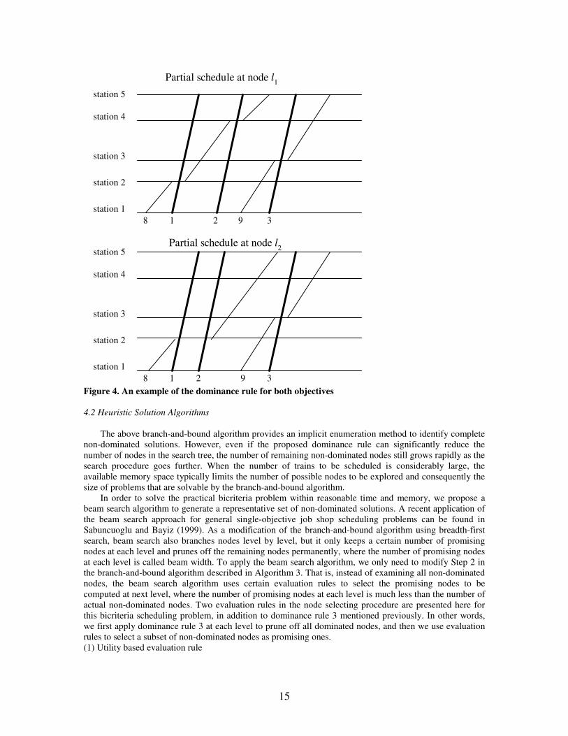
Figure 4 gives an example of the dominance rule for both objectives. Particularly, train 3 is the last scheduled high-speed train i* with )()( 2*1* ldld ii = . Both )( 1lF h and )( 2lF h include high-speed

trains 1, 2 and 3, while both )( 1lF m and )( 2lF m include medium-speed train 8. Both active sets of medium-speed trains in nodes l1 and l2 include train 9, which yields to high-speed train 3 at station 3, i.e.,

)(~

)(~

2*,1*, lklk jiji = for )( 1lAj m∈ . Furthermore, it is easy to verify that ))(())(( 2111 lFZlFZ hh <

and ))(())(( 2212 lFZlFZ mm < for these two partial schedules. According to dominance rule 3, node l1 dominates node l2.

15

Partial schedule at node l1

Partial schedule at node l2

station 5

station 4

station 3

station 2

station 1

station 5

station 4

station 3

station 2

station 18 1 2 3

8 1 2 39

9 Figure 4. An example of the dominance rule for both objectives 4.2 Heuristic Solution Algorithms

The above branch-and-bound algorithm provides an implicit enumeration method to identify complete

non-dominated solutions. However, even if the proposed dominance rule can significantly reduce the number of nodes in the search tree, the number of remaining non-dominated nodes still grows rapidly as the search procedure goes further. When the number of trains to be scheduled is considerably large, the available memory space typically limits the number of possible nodes to be explored and consequently the size of problems that are solvable by the branch-and-bound algorithm.

In order to solve the practical bicriteria problem within reasonable time and memory, we propose a beam search algorithm to generate a representative set of non-dominated solutions. A recent application of the beam search approach for general single-objective job shop scheduling problems can be found in Sabuncuoglu and Bayiz (1999). As a modification of the branch-and-bound algorithm using breadth-first search, beam search also branches nodes level by level, but it only keeps a certain number of promising nodes at each level and prunes off the remaining nodes permanently, where the number of promising nodes at each level is called beam width. To apply the beam search algorithm, we only need to modify Step 2 in the branch-and-bound algorithm described in Algorithm 3. That is, instead of examining all non-dominated nodes, the beam search algorithm uses certain evaluation rules to select the promising nodes to be computed at next level, where the number of promising nodes at each level is much less than the number of actual non-dominated nodes. Two evaluation rules in the node selecting procedure are presented here for this bicriteria scheduling problem, in addition to dominance rule 3 mentioned previously. In other words, we first apply dominance rule 3 at each level to prune off all dominated nodes, and then we use evaluation rules to select a subset of non-dominated nodes as promising ones. (1) Utility based evaluation rule

16

A commonly used idea to capture the passengers’ preferences is to consider the sum of weighted deviations from the target values of multiple objectives as an evaluation function, similar to the achievement function in goal programming. In this train scheduling problem, we can set the target values for the first and second objectives as zero variance of interdeparture times for high-speed trains, and pure traveling time without waiting, respectively. Because these two original objectives have different units, a simple summation does not reflect the true preferences of the decision maker. As mentioned previously, the variance of interdeparture times can be transformed to an out-of-vehicle waiting time measure, and the second objective is equivalent to minimizing the in-vehicle time attribute, so a multi-attribute utility theory (MAUT) model (Von Neumann and Morgenstern, 1947) is suitable for evaluating these two railroad service characteristics. Specifically, Equation (28) shows a multi-attribute utility function adopted from a discrete choice model, which has been calibrated from a study for high-speed rail in the Toronto-Montreal corridor (KPMG Peat Marwick, Koppelman, 1990). The partial solutions with high utility values will be chosen as the promising ones. It should be noted that, this function only serves as a crude evaluation, since it does not differentiate the in-vehicle time between high-speed trains and medium-speed trains, and the out-of-vehicle time in this study does not include travel time to train terminals.

U= –0.0099×(In-vehicle time) –0.0426× (Out-of-vehicle time) (28) (2) Random selection rule

Without requiring a preference model in the above method, another reasonable approach is to preserve the global trade-off information associated with the efficient frontier so that the decision maker can perform posterior analysis. We can identify the feature points in the trade-off curve, and then select the nodes that are close to those feature points in an attempt to approximate the frontier, but the feature point detection problem itself is difficult to solve. Alternatively, a simple way of capturing the shape of trade-off curves is to randomly sample the nodes in the non-dominated partial solutions at the current level. 5. Case Study

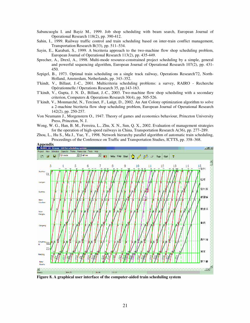
In this section, we consider the train scheduling problem for a 615 km portion of Beijing-Shanghai high-speed rail line, which consists of 17 sections between Shanghai and Xuzhou. Minimum headways range from 2 to 4 minutes, and the acceleration and deceleration times are set to 3 and 2 minutes for both high-speed and medium-speed trains, respectively. The corresponding trip, frequency and stop schedules are provided by the Fourth Survey & Design Institute of China Railway. In this study, our focus is on the interaction between 24 high-speed trains and 12 medium-speed trains in the morning period (6:00 am-12:00 am), while all the trains pass through from Shanghai to Xuzhou. Accordingly, the preferred high-speed train departure times are evenly distributed every 30 minutes. The transfer times for medium-speed trains are constructed from the existing railroad timetables. All the experiments are performed on a Pentium III PC with 600 MHz CPU and 1 GB memory, and all the algorithms are implemented in Visual C++ 6.0 on the Windows platform. A screenshot of the GUI for this train scheduling system is demonstrated in Appendix. (1) Single train scheduling algorithms

Based on the experiments with 240 instances of the single train scheduling problem, the best-first search branch-and-bound algorithm (Algorithm 2) is able to find optimal solutions in 229 instances when reaching the first feasible solutions, and the average computation time is no more than 0.1 second. The number of nodes explored by the algorithm grows dramatically as the number of sections increases, and the most time-consuming operation in the exact algorithm, essentially, is to find feasible starting time for no-stop modes. In comparison, the ZOOM solver in GAMS (Brooke et al., 2000) was used to solve the scheduling model with the second objective, taking average 2.83 seconds to find optimum for an instance with 5 sections and 7 trains. Overall, the best-first search branch-and-bound algorithm produces high-quality solutions efficiently, so it is selected to solve subproblem 3 in the following experiments. (2) Non-dominated solutions produced by exact algorithms

In order to limit the number of instances to be examined, we choose the adjustment step size as 2 minutes, and setup the maximal adjustment range for high-speed trains as +6 minutes. This allows a high-speed train to have 6+1=7 possible departure times. However, even with this relatively small adjustment range, the explicit enumeration algorithm (Algorithm 3) can only generate complete non-dominated solutions for up to 4 high-speed trains within 30 minutes. Note that, a 5 high-speed train schedule involves 75=16,807 possible solutions and each instance requires around 0.5 second even using best-first search

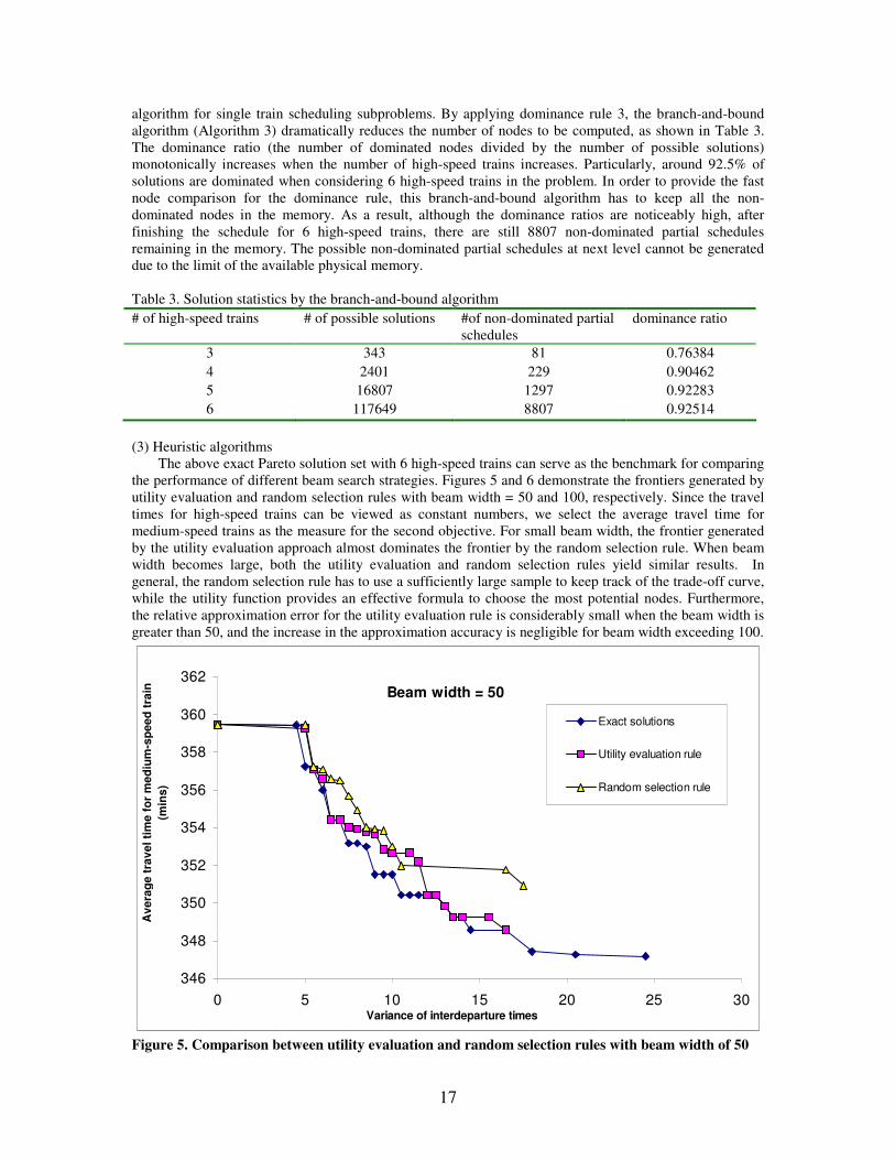
17

algorithm for single train scheduling subproblems. By applying dominance rule 3, the branch-and-bound algorithm (Algorithm 3) dramatically reduces the number of nodes to be computed, as shown in Table 3. The dominance ratio (the number of dominated nodes divided by the number of possible solutions) monotonically increases when the number of high-speed trains increases. Particularly, around 92.5% of solutions are dominated when considering 6 high-speed trains in the problem. In order to provide the fast node comparison for the dominance rule, this branch-and-bound algorithm has to keep all the non-dominated nodes in the memory. As a result, although the dominance ratios are noticeably high, after finishing the schedule for 6 high-speed trains, there are still 8807 non-dominated partial schedules remaining in the memory. The possible non-dominated partial schedules at next level cannot be generated due to the limit of the available physical memory. Table 3. Solution statistics by the branch-and-bound algorithm # of high-speed trains # of possible solutions #of non-dominated partial

schedules dominance ratio

3 343 81 0.76384 4 2401 229 0.90462 5 16807 1297 0.92283 6 117649 8807 0.92514

(3) Heuristic algorithms

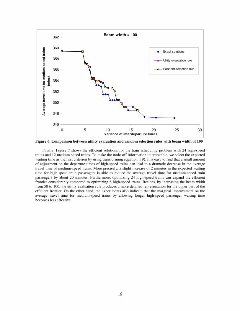
The above exact Pareto solution set with 6 high-speed trains can serve as the benchmark for comparing the performance of different beam search strategies. Figures 5 and 6 demonstrate the frontiers generated by utility evaluation and random selection rules with beam width = 50 and 100, respectively. Since the travel times for high-speed trains can be viewed as constant numbers, we select the average travel time for medium-speed trains as the measure for the second objective. For small beam width, the frontier generated by the utility evaluation approach almost dominates the frontier by the random selection rule. When beam width becomes large, both the utility evaluation and random selection rules yield similar results. In general, the random selection rule has to use a sufficiently large sample to keep track of the trade-off curve, while the utility function provides an effective formula to choose the most potential nodes. Furthermore, the relative approximation error for the utility evaluation rule is considerably small when the beam width is greater than 50, and the increase in the approximation accuracy is negligible for beam width exceeding 100.

Beam width = 50

346

348

350

352

354

356

358

360

362

0 5 10 15 20 25 30Variance of interdeparture times

Ave

rage

trav

el ti

me

for

med

ium

-spe

ed tr

ains

(m

ins)

Exact solutions

Utility evaluation rule

Random selection rule

Figure 5. Comparison between utility evaluation and random selection rules with beam width of 50

18

Beam width = 100

346

348

350

352

354

356

358

360

362

0 5 10 15 20 25 30Variance of interdeparture times

Ave

rage

trav

el ti

me

for

med

ium

-spe

ed tr

ains

(m

ins)

Exact solutions

Utility evaluation rule

Random selection rule

Figure 6. Comparison between utility evaluation and random selection rules with beam width of 100

Finally, Figure 7 shows the efficient solutions for the train scheduling problem with 24 high-speed trains and 12 medium-speed trains. To make the trade-off information interpretable, we select the expected waiting time as the first criterion by using transforming equation (19). It is easy to find that a small amount of adjustment on the departure times of high-speed trains can lead to a dramatic decrease in the average travel time of medium-speed trains. More precisely, a slight increase of 2 minutes in the expected waiting time for high-speed train passengers is able to reduce the average travel time for medium-speed train passengers by about 20 minutes. Furthermore, optimizing 24 high-speed trains can expand the efficient frontier considerably compared to optimizing 6 high-speed trains. Besides, by increasing the beam width from 50 to 100, the utility evaluation rule produces a more detailed representation for the upper part of the efficient frontier. On the other hand, the experiments also indicate that the marginal improvement on the average travel time for medium-speed trains by allowing longer high-speed passenger waiting time becomes less effective.

19

335

340

345

350

355

360

365

14.5 15 15.5 16 16.5 17 17.5

Expected waiting time for high-speed trains (mins)

Ave

rag

e tr

avel

tim

e fo

r m

ediu

m-s

pee

d t

rain

s (m

ins)

Exact solutions for 6 high-speed trains

Utility evaluation rule for 24high-speed trains w ith beamw idth = 50

Utility evaluation rule for 24high-speed trains w ith beamw idth = 100

Figure 7. Trade-off curves for the first and second objectives 6. Conclusions

Train scheduling is an important component in optimizing the performance of the railroad industry. This paper highlights the potential of using multi-objective scheduling methods to generate Pareto solutions and corresponding trade-offs for railroad timetable planning applications. The contributions of this study are as follows. First, a bicriteria train scheduling model is proposed to optimize and balance in-vehicle travel time and out-of-vehicle waiting time simultaneously by aid of the random incidence theorem. Second, a multi-mode scheduling model with exact and efficient heuristic algorithms is developed for the train scheduling problem considering acceleration and deceleration features. Furthermore, an implicit enumeration algorithm with effective dominance rules and a beam search algorithm with the utility evaluation rule are proposed to generate Pareto optimal solutions and corresponding representative sets.

As an implementation using CPLEX (ILOG, 2001) is underway, other future research directions include (1) how to extend the proposed multi-objective framework to a general rail line, which should also consider the requirements for freight demand, (2) how to interact with the decision maker to obtain his/her preference information so as to improve the effectiveness of the beam search algorithm with utility evaluation rules, and (3) how to incorporate the out-of-vehicle waiting time for scheduled arrivals. It is also desirable to use stochastic optimization techniques to consider the possible adjustment and variations for the transfer times of medium-speed trains at the connecting stations. 7. Acknowledgements

This paper is based in part on previous research funded by the Fourth Survey & Design Institute of China Railway. The study has benefited from the comments from Anliang Xie and Hayssam Sbayti, and the encouragement and support by Dr. Hani. S. Mahmassani. The authors would also like to thank two anonymous referees for their constructive suggestions, which improved the content substantially. The authors are of course responsible for all results and opinions expressed in this paper. References Adenso-Diaz, B., Gonzalez, M. O., Gonzalez-Torre, P., 1999. On-Line timetable re-scheduling in regional

train services, Transportation Research B(33), pp. 387–398. Assad, A., 1980. Models for rail transportation, Transportation Research A(14), pp. 205–220.

20

Bhat, C., 1995. A heteroscedastic extreme value model of intercity travel mode choice, Transportation Research B(29), pp.471–483.

Brannlund, U., Lindberg, P.O., Nou, A., Nilsson, J. E., 1998. Railway timetabling using Lagrangian relaxation, Transportation Science 32, pp. 358–369.

Brooke, A., Kendrick, D., Meeraus, A., 2000. GAMS - A user's guide (Release 2.50), The Scientific Press, Redwood City, CA.

Brucker, P., Drexl, A., Mohring, R., Newmann, K., Pesch, E., 1999. Resource-constrained project scheduling: Notation, classification, models, and methods, European Journal of Operational Research 112(1), pp. 3–41.

Bussieck, M. R., Kreuzer, P., Zimmermann, U. T., 1997. Optimal lines for railway systems, European Journal of Operational Research 96(1), pp. 54–63.

Cai, X., Goh, C. J., Mees, A. I., 1998. Greedy heuristics for rapid scheduling of trains on a single track, IIE Transactions 30, pp. 481–493.

Chang,Y.H., Yeh, C.H., Shen, C.C., 2000. A multiobjective model for passenger train services planning: application to Taiwan's high-speed rail line, Transportation Research B(34), pp. 91–106.

Cordeau, J.-F., Toth, P., Vigo, D., 1998. A survey of optimization models for train routing and scheduling, Transportation Science 32, pp. 380–404.

Framinan, J. M., Leisten, R., Ruiz-Usano, R., 2002. Efficient heuristics for flowshop sequencing with the objectives of makespan and flowtime minimization, European Journal of Operational Research 141(3), pp. 559-569.

Greenberg, H.H., 1968. A branch and bound solution to the general scheduling problem, Operations Research 16, pp. 352– 361.

Higgins, A., Kozan, E., Ferreira, L., 1996. Optimal scheduling of trains on a single line track, Transportation Research B(30), pp. 147–161.

Higgins, A., Kozan, E., 1998. Modeling train delays in urban networks, Transportation Science 32, pp. 346–357.

ILOG, 2001. ILOG Cplex 7.1, Reference Manual. Kraay, D. R., Harker, P. T., 1995. Real-time scheduling of freight railroads, Transportation Research B(29),

pp. 213–229. Kraft, E. R., 1987. A branch and bound procedure for optimal train dispatching, Journal of the

Transportation Research Forum 28 (1), pp. 263-276. Kraft, E. R., 1998. A reservations-based railway network operations management system, Ph. D.

Dissertation, Department of Systems Engineering, University of Pennsylvania, Philadelphia, PA. KPMG Peat Marwick, Koppelman, F.S., 1990. Analysis of the market demand for high speed rail in the

Quebec–Ontario corridor, Report produced for Ontario/Quebec Rapid Train Task Force, KPMG Peat Marwick, Vienna, VA.

Larson, R., Odoni, A., 1981. Urban operations research, Prentice-Hall, NJ. Ma, J., Hu, S., Xu, H., Fan, J., 2002. A multi-objective model for train working diagram for Jinghu high-

speed train line, Proceedings of the Third International Conference on Traffic and Transportation, ICTTS, Beijing, pp.350–355.

Nagar, A., Haddock, J., Heragu, S., 1995. Multiple and bicriteria scheduling: A literature survey, European Journal of Operational Research 81 (1), pp. 88–104.

Nazareth, T., Verma, S., Bhattacharya, S., Bagchi, A., 1999. The multiple resource constrained project scheduling problem: A breadth-first approach, European Journal of Operational Research 112(2), pp. 347-366.

Neppalli, V. R., Chen, C.-L., Gupta, J.N.D., 1996. Genetic algorithms for the two-stage bicriteria flow shop problem, European Journal of Operational Research 95(2), pp. 356–373.

Nie, L., Hu, A., Zhang, X., 2000. Simulation analysis of traffic organization on high speed railway, Proceedings of the Second International Conference on Traffic and Transportation, ICTTS, Beijing, pp.929–934.

Patterson, J. H., Slowiski, R., Talbot, F. B., Weglarz, J., 1990. Computational experience with a backtracking algorithm for solving a general class of resource constrained scheduling problems, European Journal of Operational Research 90(1), pp. 68–79.

Patterson, J. H., Slowiski, R., Talbot, F. B., Weglarz, J., 1989. An algorithm for a general class of precedence and resource constrained scheduling problems, Advances in Project Scheduling, Elsevier, pp. 3–28.

21

Sabuncuoglu I. and Bayiz M., 1999. Job shop scheduling with beam search, European Journal of Operational Research 118(2), pp. 390-412.

Sahin, I., 1999. Railway traffic control and train scheduling based on inter-train conflict management, Transportation Research B(33), pp. 511–534.

Sayin, E., Karabati, S., 1999. A bicriteria approach to the two-machine flow shop scheduling problem, European Journal of Operational Research 113(2), pp. 435-449.

Sprecher, A., Drexl, A., 1998. Multi-mode resource-constrained project scheduling by a simple, general and powerful sequencing algorithm, European Journal of Operational Research 107(2), pp. 431-450.

Szpigel, B., 1973. Optimal train scheduling on a single track railway, Operations Research'72, North-Holland, Amsterdam, Netherlands, pp. 343–352.

T'kindt, V., Billaut, J.-C., 2001. Multicriteria scheduling problems: a survey, RAIRO - Recherche Opérationnelle / Operations Research 35, pp.143-163.

T’kindt, V., Gupta, J. N. D., Billaut, J.-C., 2003. Two-machine flow shop scheduling with a secondary criterion, Computers & Operations Research 30(4), pp. 505-526.

T’kindt, V., Monmarché, N., Tercinet, F., Laügt, D., 2002. An Ant Colony optimization algorithm to solve a 2-machine bicriteria flow shop scheduling problem, European Journal of Operational Research 142(2), pp. 250-257.

Von Neumann J., Morgenstern O., 1947. Theory of games and economics behaviour, Princeton University Press, Princeton, N. J.

Wong, W. G., Han, B. M., Ferreira, L., Zhu, X. N., Sun, Q. X., 2002. Evaluation of management strategies for the operation of high-speed railways in China, Transportation Research A(36), pp. 277–289.

Zhou, L., Hu S., Ma J., Yue, Y., 1998. Network hierarchy parallel algorithm of automatic train scheduling, Proceedings of the Conference on Traffic and Transportation Studies, ICTTS, pp. 358–368.

Appendix

Figure 8. A graphical user interface of the computer-aided train scheduling system