Beyond the Normal Stellar Atmosphere

II ⋅ Stellar Atmospheres

Copyright (2003) George W. Collins, II

16

Beyond the Normal Stellar Atmosphere

. . . With the exception of a few subjects in Chapter 7, we have dealt exclusively with spherical stars throughout this book. In addition, these stars have been "normal" stars; that is, they are stars without strange peculiarities or large time-dependent effects in their spectra. These are stars, for the most part, with interiors evolving on a nuclear time scale and atmospheres which can largely be said to be in LTE. The prototypical star that fits this description is a main sequence star, and for such stars the theoretical framework laid down in this book will serve quite well as a basis for understanding their structure and spectra. However, the notion of a spectral peculiarity is somewhat "in the eye of the beholder". Someone who looks closely at any star will find grounds for calling it peculiar or atypical. This is true of even the main sequence stars, and we would delude ourselves if we believed that all aspects of any star are completely understood.

432

16 ⋅ Beyond the Normal Stellar Atmosphere

Phenomena are known to exist in the atmospheres of stars that we have not included in the basic theory. For example, convection does exist in the upper layers of late-type stars and contributes to the transport of energy. However, the efficiency of this transport is vastly inferior to that which occurs in the stellar interior, because the mean free path for a convective element is of the order of that for a photon. Nevertheless, in the lower sections of the atmosphere, convection may carry a significant fraction of the total energy. Unfortunately, the crude mixing length theory of convective transport that was effective for the stellar interior is insufficient for an accurate description of atmospheric convection. The turbulent motion exhibited by the atmospheres of many giant stars also represents the transport of energy and momentum in a manner similar to convection. Just the kinetic energy of the turbulent elements themselves should contribute significantly to the pressure equilibrium in the upper atmosphere. However, if one naively assigned a turbulent pressure of ρv2 to the elements, the measured turbulent velocities would imply a pressure greater than the total pressure of the gas and the atmosphere would be unstable. Clearly a better theory of turbulence is required before any significant progress can be made in this area. In the last 20 years, it has become clear that the atmospheres of many stars are indeed unstable. Ultraviolet observations of the spectra of early-type stars suggest that they all possess a stellar wind of out-flowing matter of significant proportions. As one moves upward in the atmosphere of a star, departures from LTE increase to such a point that they dominate the atmospheric structure. In addition, energy sources such as magnetic fields, atmospheric mass motions, and possibly acoustic waves associated with convection or turbulence may contribute significantly to the higher level structure. While these energy contributions are tiny when compared to the energy densities in the photosphere, the contributions may supply the majority of the interaction energy between the star and its outermost layers which are basically transparent to photons. In the hottest stars, the pressure of radiation, transmitted to the rarefied upper layers of the atmosphere through absorption by the resonance lines of metals, will cause this low-density region to become unstable, expand, and eventually be driven away. This is undoubtedly the source of the stellar winds for stars on the upper main sequence and in the early-type giants and supergiants. The extended atmospheres of these stars pose an entirely new set of problems for the theory of stellar atmospheres. Many stars exist in close binary systems so that the atmosphere of each is exposed to the radiation from the other. In some instances, the illuminating radiant flux from the companion may exceed that of the star. Under these conditions we can expect the local atmospheric structure to be dominated by the external source of

433


radiation. In addition, such stars are liable to be severely distorted from the spherical shape of a normal star. This implies that the defining parameters of the stellar atmosphere (µ, g, and Te) will vary across the surface. Even in the absence of a companion, rapid rotation of the entire star can provide a similar distortion with the accompanying variation of atmospheric parameters over the surface. These are some of the areas of contemporary research and to even recount the present state of progress in them would require another book. Instead of skimming them all, in this last chapter, we consider one or two of them in the hopes of pricking the reader's interest to find out more and perhaps contribute to the solution of some of these problems. 16.1 Illuminated Stellar Atmospheres Although the majority of stars exist in binary systems, and many of them are close binary systems, little attention has been paid to the effects on a stellar atmosphere, by the illuminating radiation of the companion. The general impact of this illumination on the light curve of an eclipsing binary system has usually been lumped under the generic term "reflection effect". This is a complete misnomer, for most of any incident energy is absorbed by the atmosphere and then reradiated. Only that fraction which is scattered could, in any sense, be considered to be reflected and then only that fraction that is scattered in the direction of the observer. a Effects of Incident Radiation on the Atmospheric Structure The presence of incident radiation introduces an entirely new set of parameters into the problem of modeling a stellar atmosphere. Basically the incident radiation will be absorbed in the atmosphere, causing local heating. The amount of this heating will depend on the intensity, direction, and frequency of the incident radiation as well as the fraction of the visible sky covered by the source. This local heating can totally alter the atmospheric structure causing the appearance of the illuminated star to change greatly. However, if radiative equilibrium is to apply, all the radiation that falls on the star must eventually emerge. The interaction of the incident radiation with the atmosphere will cause its spectral energy distribution to be significantly altered. In any event, the total emergent flux must simply be the sum of the incident flux and that which would be present in the unilluminated star. In addition to this being the common sense result, it is a consequence of the linearity of the equation of radiative transfer. Before we can even formulate an equation of radiative transfer appropriate for an illuminated atmosphere, we must know the angular distribution of the incident energy. For simplicity, let us assume that the incident radiation comes from some known direction (θ0, φ0) in the form of a plane wave (see Figure 16.1). 434


Figure 16.1 shows radiation incident on a plane-parallel atmosphere.

The radiation can be specified as coming from a specific direction indicated by the coordinates 00 ,φθ .

The specific intensity incident on the atmosphere can then be characterized by

(16.1.1) where Fi is the incident flux and the δ(xi) is the Dirac delta function indicating the direction of the beam. Along an optical path τν/µ0, this radiation will be attenuated by

. Chandrasekhar0/ µτ− νe 1 makes a distinction between the direct transmitted intensity and that part of the radiation field (the diffuse field) that has been scattered at least once. The contribution to the diffuse radiation field from the attenuated incident radiation field is

(16.1.2) where εν is the fraction of the intensity absorbed in a differential length of the optical path and has the same meaning as in equation (10.1.8). This can be regarded as the scattering contribution to the diffuse source function from the attenuated incident radiation field. Thus the equation of radiative transfer for the illuminated atmosphere is

435


(16.1.3) By applying the classical solution to the equation of transfer, we can generate an integral equation for the diffuse field source function, as we did in (Section 10.1) so that

(16.1.4)

This is a Schwarzschild-Milne integral equation of the same type as we considered in Chapter 10 it and can be solved in the same manner. The only difference is that the term that makes the equation inhomogeneous has been augmented by the last term on the right in equation (16.1.4). Thus the presence of incident radiation will even make a pure scattering atmosphere inhomogeneous and subject to a unique solution. Modification of the Avrett-Krook Iteration Scheme for Incident Radiation. Buerger2 has solved this equation, using the ATLAS atmosphere program for a variety of cases. He found that the standard Avrett-Krook iteration scheme described in Section 11.4 would no longer lead to a converged atmosphere. This is not surprising since the Eddington approximation was used to obtain the specific perturbation formulas (see equations (12.4.17), (12.4.25), and (12.4.29), and the approximation J(0) = ½F(0) will no longer be correct. Buerger therefore adopted a modification of the Avrett-Krook scheme due to Karp3 which replaces the ad hoc assumption of equations (12.4.14) and (12.4.20) with

(16.1.5) which implies that

(16.1.6) He continues by making the plausible assumption that perturbed flux variations have the same frequency dependence as the zeroth-order flux variations so that

(16.1.7) Following the same procedure as Karp, Buerger2 finds the perturbation formulas for τ(1) and T(1) analogous to equations (12.4.21) and (12.4.29), respectively, to be

436


(16.1.8) where

(16.1.9) While these equations do provide a convergent iteration algorithm, the rate of convergence can be quite slow if the amount of incident radiation is large and differs greatly from that which the illuminated star would have in the absence of incident radiation. If event that the incident flux has an energy distribution significantly different from that of the illuminated star and large compared to the stellar flux, the Eddington approximation will fail rather badly at some frequencies and in that part of the atmosphere where the majority of the incident flux is absorbed. Under these conditions, the Avrett-Krook iteration scheme will fail badly. Steps must be taken to directly estimate those parameters obtained from the Eddington approximation. In some instances it is possible to use results from a previous iteration. Initial Temperature Distribution As with any iteration process, the closer the initial guess, the faster a correct answer will be found. In Chapter 12, we suggested that the model-making process could be initiated with the unilluminated gray atmosphere temperature distribution in the absence of anything better. In the case of incident radiation, such a choice will yield an initial temperature distribution that departs rather badly from the correct one. It is tempting to suggest that a suitable first guess could be obtained by merely scaling up the gray atmosphere temperature distribution so as to include the incident flux in the definition of the effective temperature. Thus,

(16.1.10) where Te(0) is the effective temperature and the temperature distribution is

437


(16.1.11) Here q(τ) is the Hopf function defined in Chapter 10 [equation (10.2.33)]. For the Eddington approximation,

(16.1.12) However, there are two effects that make this a poor choice. First, if the sky of the illuminated star is partially filled with the illuminating star, then much of the incident radiation will enter at a grazing angle and preferentially heat the upper atmosphere. This will raise the surface temperature over what would normally be expected from a gray atmosphere and will flatten the temperature gradient. The more radiation that enters from grazing angles, the greater this effect will be. This effect may also be understood by considering how radiation can ultimately escape from the atmosphere. If the source of radiation is a close companion filling much of the sky, then a smaller and smaller fraction of the sky is "black" representing directions of possible escape. As the possible escape routes for photons diminish, the atmosphere will heat up since the photons have nowhere to go. Anderson and Shu4 suggest that this may be compensated for by

(16.1.13) where Ω0 is the solid angle subtended by the source of radiation in the sky. As Ω0 → 0, we recover the Eddington approximation's value for Q0. As Ω0 increases, so does the value of Q0 implying that the surface temperature will rise relative to the effective temperature. In the limit, the atmosphere will approach being isothermal. The second aspect of incident radiation that can markedly affect the temperature distribution is the frequency distribution. If the source of the incident radiation contains a large quantity of ionizing radiation and is incident on a relatively cool star, then almost all the radiation will be absorbed by the neutral hydrogen of the upper reaches of the atmosphere, raising the local temperature significantly. Similarly, if the incident radiation is highly penetrating radiation, such as x-rays, the heating may occur much lower in the atmosphere. Since this energy must be reradiated, this will result in a general elevation of the entire atmospheric temperature distribution. This dependence of the atmosphere's temperature gradient on the frequency distribution makes predicting the outcome extremely difficult since the process is highly nonlinear. That is, the local heating may change the opacity, which will in turn change the heating.

438


In general, incident radiation will preferentially heat the surface layers and a modification like that suggested by Anderson and Shu4 should be used for the initial guess. An additional approach that some investigators have found useful is to slowly increase the amount of incident radiation during the iteration processes from an initially low value until the desired level is reached. The rate at which this can be done depends on the spectral energy distribution of the incident radiation and always tends to lengthen the convergence process. b Effects of Incident Radiation on the Stellar Spectra If the amount of this illuminating radiation is large, then the heating of the upper atmosphere will cause a decrease in the temperature gradient. As we have seen in Chapter 13, the strength of a pure absorption line will depend strongly on the temperature gradient in the atmosphere. Thus, aside from changes in the environment of the radiation field caused by the external heating, we should expect spectral lines to appear weaker simply because of the change in the source function gradient. The change in line strength may cause an attendant change in the spectral type. Although such changes should be phase dependent in a binary system, as different aspects of the illuminated surface are presented to the observer, such changes can be confused with the contribution to the light by the companion. Although Milne5 first laid the foundations for estimating these effects in 1930, very little has been done in the intervening half-century to quantify them. The atmospheres investigated by Buerger2 did indeed show the general decrease in the equivalent widths of the lines investigated due to heating of the higher levels of the atmosphere. However, his investigation was restricted to point-source illumination which tends to minimize the upper-level heating of the atmosphere. A more realistic modeling of the atmosphere of an early-type binary system by Kuzma6 showed that the effects can be quite pronounced. Local changes of the atmospheric structure can produce spectral changes of several spectral subtypes with the integrated effect being as large as several tenths of a subtype with phase. The effects of the incident radiation on the spectra become deeply intertwined with the structure. The inclusion of metallic line blanketing brought about a reversal of the effects of non-LTE on the hydrogen lines in that, in the upper levels of the atmosphere, the departure coefficients for the first two levels of hydrogen (b1 and b2) went from about 0.6 to 1.5 when the effects of line blanketing were included. Similar anomalies occurred for the departure coefficients for the higher levels as well. This fact largely serves to show the interconnectedness of the phenomena which earlier we were able to consider separately. This results primarily from the dominance of the interactions of the gas with the radiation field over interactions with itself. That is, the radiation field and its departures from statistical

439


equilibrium begin to determine completely the statistical equilibrium of the gas. The illuminating radiation has a spectral energy distribution significantly different from that of the illuminating star, the departures from LTE may be very large indeed. 16.2 Transfer of Polarized Radiation Even before the advent of classical electromagnetism in 1864 by James Clerk Maxwell, it was generally accepted that light propagated by means of a transverse wave. Any such wave would have a preferred plane of vibration as seen by an observer, and any collection of such beams that exhibited such a preferred plane was said to be polarized. In 1852, George Stokes7 showed that such a collection of light beams could be characterized by four parameters that now bear his name. Normally a heterogeneous collection of light beams will have planes of oscillation that are randomly oriented as seen by an observer and will be called unpolarized. However, should a light beam exhibit some degree of polarization, a measure of that polarization potentially contains a significant amount of information about the nature of the source. This property of light has been largely ignored in stellar astrophysics until relatively recently. The probable reason can be found in the assumption that all stars are spherical. Any such object would be completely symmetric about the line of sight from the observer to the center of the apparent disk so if even local regions on the surface emitted 100 percent polarized light, the symmetric orientation of their planes of polarization would yield no net polarization to an observer viewing the integrated light of the disk. However, many astrophysical processes produce polarized light, and numerous stars are not spherical. In particular, eclipsing binary systems present a source of integrated light which is not symmetric about the line of sight. Early work by Chandrasekhar8,9 and Code10 implied that there might be measurable polarization that would place significant constraints on the nature of the source. However, only after the development of very sensitive detectors and the discovery of intrinsic circular polarization in white dwarfs did intrinsic stellar polarization attract any great interest. In the hope that this interest will continue to grow, we will discuss some of the theoretical approaches to the problems posed by the transfer of polarized light. a Representation of a Beam of Polarized Light and the Stokes

Parameters Imagine a collection of largely uncorrelated electromagnetic waves propagating in the same direction through space. The combined effect of these beams can be obtained by adding the squares of the amplitudes of their oscillating electric and magnetic vectors. If the waves were completely correlated as are those from a laser, the amplitudes themselves would vectorially add directly. Indeed, the representation of the addition of the squares of the amplitudes can be taken as a 440


definition of a completely uncorrelated set of waves. Now consider a situation where the collection of waves interacting with some object that produces a systematic effect on the waves such as a phase shift that depends on the orientation of the wave to the object. A reflection from a mirror produces such an effect. If we introduce a coordinate system to represent this interaction (see Figure 16.2), the net effect of summing components of the amplitudes of the combined waves could produce an ellipse whose orientation changes as it propagates through space. Such a beam is said to be elliptically polarized. If the tip of the combined electric vectors appears to rotate counterclockwise as viewed by the observer, the beam is said to have positive helicity or to be left circularly polarized. However, some authors define the state of positive polarization to be the reverse of this convention, and students should be careful, when reading polarization literature, which is being employed by the author.

Figure 16.2 shows two beams of light incident on a reflecting surface where a phase shift is introduced between those with electric vectors vibrating parallel to the surface and those vibrating normal to the surface. The combined effect on the two beams is to have initially unpolarized light converted into an elliptically polarized beam.

441


In 1852, George Stokes7 showed that such a beam of light could be represented by four quantities. Although we now use a somewhat different notation than that of Stokes, the meaning of those parameters is the same. Basically, the four parameters required to describe a polarized beam are the total intensity; the difference between two orthogonal components of the intensity, which is related to the degree of polarization; the orientation of the ellipse, which specifies the plane of polarization; and the degree of ellipticity, which is related to the magnitude of the systematic phase shifts introduced by the interaction that gives rise to the polarized beam. Since these quantities presuppose the existence of the coordinate system for their definition, they can be defined most easily in terms of those coordinates (see Figure 16.2) as

(16.2.1) where Tanβ is the ratio of the semi-minor to the semi-major axis of the ellipse. The quantities El and Er are the amplitudes of two orthogonal waves that are phase shifted by ε. The vector superposition of two such waves will produce a single wave with an amplitude that rotates as the wave moves through space. We will take 0 ≤ β ≤ π/2, and the whether sign of β is positive or negative will determine if the beam is to be called left or right elliptically polarized respectively. If Q = U = V = 0, the light is said to be completely unpolarized, while if V = 0, the beam is linearly polarized with a plane of polarization making an angle χ with the l-axis. Since the Stokes parameters contain some information which is purely geometric, we should not be surprised if, for a completely polarized beam, the parameters are not linearly independent and that relationships exist between them involving their geometric representation. Specifically, from equations (16.2.1) we get

(16.2.2) Since the Stokes parameters already involve combining the squares of the amplitudes of an arbitrary beam, we should be able to add a natural or unpolarized beam directly to the completely polarized beam. For such a beam Il = Ir in all coordinate systems and Q = U = V = 0, so that

(16.2.3)

442


Thus for a collection of light beams, some of which may be polarized, all four Stokes parameters are indeed linearly independent and must be specified to completely characterize the beam. It is clear from the definitions of the Stokes parameters that I and V are invariant to a coordinate rotation about the axis of propagation while Q and U are not. If we rotate the l-r coordinate frame through an angle φ in a counterclockwise direction (see Figure 16.2), then

(16.2.4) Since I and V are invariant to rotational transformations, we can write the general rotation for the Stokes parameters in matrix-vector notation. If we define an intensity vector to have components I

r[I,Q,U,V] so that

(16.2.5) then we can call the matrix the rotation matrix for the Stokes parameters. If we choose a coordinate system so that Il is a maximum, then the degree of linear polarization P is a useful parameter defined by

(16.2.6) where, since the l-r coordinate frame has been chosen so that the l-axis lies along this direction of maximum intensity, U = 0. It is also useful to linearly decompose the Stokes parameters I and Q into Il and Ir so that

(16.2.7) However, neither of these parameters is invariant to a coordinate rotation so that if we denote a vector I

r(Il,Ir,U,V) whose components are this different set of Stokes

parameters, then

(16.2.8) where the rotation matrix for these Stokes parameters is

443


(16.2.9) The rotation matrix L(φ) can be obtained from equation (16.2.5) by employing the definitions of I and Q in terms of Il and Ir in equation (16.2.7). Here the angle φ is taken positively increasing for counterclockwise rotations. While this definition is the opposite of that used by Chandrasekhar1 (p. 26), it is the more common notation for a rotational angle. The form of this rotation matrix is a little different from that used to transform vectors because the quantities being transformed are the squares of vector components rather than the components and their composition law is different from that for vectors alone. However, the transformation matrix does share the common group identities of the normal rotation matrices so that

(16.2.10) Finally, there is an additional way to conceptualize the Stokes parameters that many have found useful. In general, a polarized beam of light can be imagined as being composed of two orthogonally oscillating electric vectors bearing a relative phase shift e with respect to one another. The vector sum of these two amplitudes will be a vector whose tip traces out an elliptically helical spiral as the vector propagates through space. We have defined the Stokes parameters in terms of the projection of that spiral onto a plane normal to the direction of propagation. However, we can also view them in terms of the motion of the vector through space. The fact that the vector rotates results from the phase difference between the two waves. If the phase difference were an odd multiple of π/2, then the wave would spiral through space and would be said to contain a significant amount of circular polarization. However, if the phase difference e were zero or a multiple of π, the tip of the vector would merely oscillate in a plane whose orientation is determined by the ratio of the amplitudes of the electric vectors in the original orthogonal coordinate frame defining the beam, and the beam would be said to be linearly polarized. Since the Stokes parameters are intensity-like (i.e. they have they units of the square of the electric field), one way to identify them is to take the outer (tensor) product of the electric vector with itself. Such an electric vector will have components El and Er so that the outer product will be

(16.2.11) 444


Only three of these components are linearly independent, but the component Er itself is made up of two linearly independent components Ercosε and Ersinε. Thus the expansion of the term ElEr leaves us with four intensity-like components which we can identify with the Stokes parameters so that formally

(16.2.12) Thus taking the outer product of a general electric vector provides an excellent formalism for generating the Stokes parameters for that beam. b Equations of Transfer for the Stokes Parameters The intensity-like nature of the Stokes parameters that describe an arbitrarily polarized beam makes them additive. This and the linear nature of the equation of radiative transfer ensures that we can write equations of transfer for each of them. Thus, if the components of I

rare the Stokes parameters, we can express this

result as a vector equation of radiative transfer that has the familiar form

(16.2.13) As usual, all the problems in the equations of transfer are contained in the source function. If we choose the intensity vector to have components I

r[Il,Ir,U,V], then the

source function can be written as a vector whose components are Sl, Sr, SU, and SV. Again, as we did with incident radiation, it is convenient to break up the radiation field into the "diffuse" field consisting of photons that have interacted at least once and the direct transmitted field that could originate from any incident radiation. We concentrate initially on the diffuse field since, in the absence of incident radiation, it exhibits axial symmetry about the normal to the atmosphere. Nature of the Source Function for Polarized Radiation The source function that appears in equation (16.2.13) is a vector quantity that must account for all contributions to the four Stokes parameters from thermal and scattering processes. Since thermal emission is by nature a random equilibrium process, we expect it to make no contribution to the Stokes parameters U and V for these measure the departure of the radiation field from isotropy but now carry energy. In short, thermal radiation is completely unpolarized. For the same reasons, the thermal radiation will make an equal contribution to both Il and Ir. Therefore the thermal contribution to the vector source function in equation (16.2.13) will have components

445


(16.2.14) where εν is the familiar ratio of pure absorption to total extinction defined in equation (10.1.8). In some instances it is possible for εν to depend on orientation. This is particularly true if an external magnetic field is present. The role played by scattering is considerably more complex. Redistribution Phase Function for Polarized Light For the sake of simplicity, let us assume that the scattering is completely coherent so that there is no shift in the frequency of the photon introduced by the scattering process. However, in some instances scattering can result in photons being scattered from the l-plane into the r-plane, so that in principle all four Stokes parameters may be affected. In addition, the scattering by the atom or electron is most simply described in the reference frame of the scatterer and most simply involves the angle between the incoming and outgoing photons. But the coordinate frame of the equation of transfer is affixed to the observer. Thus we must express not only the details by which the photons are scattered from one Stokes parameter to another, but also that result in the coordinate frame of the equation of radiative transfer. It is this latter transformation that took the relatively simple form of the Rayleigh phase function and turned it into the more complicated form given by equation (15.3.39). Since the scattering of a photon may carry it from one Stokes parameter to another, we can expect the redistribution function to have the form of a matrix where each element describes the probability of the scattering carrying the photon from some given Stokes parameter to another. We have already seen that the tensor outer product provides a vehicle for identifying the Stokes parameters in a beam. Let us use this formalism to investigate the Stokes parameters for a polarized beam of light scattered by an electron. While we generally depict a light beam as being composed of a single electric vector oscillating in a plane, this is not the most general form that a light wave can have. Consider a beam of light composed of orthogonal electric vectors and '

lEr

'rEr

' which are systematically phase-shifted with respect to each other. Let this beam be incident on an electron so that the wave is scattered in the l-plane (see Figure 16.3). We are free to pick the l-plane to be any plane we wish, and the scattering plane is a convenient one. We can also view the scattering event to result from the acceleration of the electron by the incident electric fields '

lEr

and 'rEr

producing oscillating dipoles which reradiate the incident energy. Since the photon is reradiated in the l-plane, we may consider it to be made up of electric vectors lE

r and rE

rwhich bear the same

relative phase shift to each other as 'lEr

and 'rEr

. Now consider how each dipole

446


excited by and 'lEr

'rEr

will re-radiate in the scattering plane. In general, electric dipoles will radiate in a plane containing the dipole axis, but the amplitude of that wave will decrease as one approaches the pole, specifically as the sine of the polar angle. Thus the intensity of

rwill vary as cosγ while lE rE

rwill be independent of the

scattering (see Figure 16.3). Thus the scattered vector Er

will have components

[ cosγ, ]. Taking the outer product of this vector with itself, we can identify the linearly independent components as

'lEr

'rEr

(16.2.15)

447

Figure 16.3 shows the electric vectors of two orthogonal waves differing in phase by ε incident on an electron. The scattering of the waves takes place in the same plane as the oscillating

r

wave. The angle through which the waves are scattered is γ. Each wave can be viewed as exciting a dipole which radiates in the scattering plane in accordance with dipole radiation for the orientation of the respective dipoles.

'lE


Since the dipoles excited by the incident radiation do not reradiate in a plane orthogonal to the exciting radiation, there can be no mixing of energy from the r-plane to the l-plane or vice versa. Thus, in any scattering matrix for Stokes parameters, the four independent components of the beam given by equation (16.2.15) must appear on the diagonal. In addition, one would expect a constant of proportionality determined by the conservation of energy. Specifically, the total energy of the incident beam must equal the total energy of radiation scattered through all allowed scattering angles. Thus, factoring out the definitions of the Stokes parameters from the components given in equation (16.2.15), we can write

(16.2.16) where A0 is the constant of proportionality described above. By applying the conservation of energy, A0 can be found to be 3/2. Thus the matrix in equation (16.2.16) represents the transformation of I

r[I'l, I', U',V'] into I

r[Il, Ir, U,V]. This

matrix is generally called the Rayleigh phase matrix and is

(16.2.17) Here γ is the scattering angle between the incoming and outgoing photons. The Stokes parameters in the scattering coordinate system will be given by the vector components of the intensity

r[II l, Ir, U, V] where Il and Ir lie in the scattering plane

and perpendicular to it in a plane containing the outgoing photon (see Figure 16.3 and Figure 16.4). The equivalent matrix for scattering of the more common Stokes vector

r'[I', Q', U', V'] to

r[I, Q, U, V] can be obtained by transforming equation

(16.2.17) in accordance with the definitions given in equation (16.2.7) so that I I

(16.2.18) To be useful for radiative transfer, these matrices must now expressed in the observer's coordinate frame by multiplying them by the appropriate rotation matrix as given in equation (16.2.9) or (16.2.5).

448


Figure 16.4 shows the coordinate frame for a single scattering event

and the orientation of the polarized components. The final transformation to the coordinate system of the equation of transfer is moderately complicated (see Chandrasekhar1, pp.37- 41) and I will simply quote the result for equation (16.2.17), using his notation.

(16.2.19) where

449


(16.2.20) The equivalent matrix for the describing the scattering of 'I

r[I',Q',U',V'] can

be obtained by transforming the matrix given in equation (16.2.19) in accordance with the definitions given in equations (16.2.7)(see equation 16.2.37). Thus the scattering matrix can be obtained in the observer's frame for either representation of the Stokes parameters. In cases where the scattering matrix may have a more complicated representation in the frame of the scatterer, it may be easier to accomplish the transformation to the observer's coordinate frame for the orthogonal electric vectors themselves and then reconstruct the appropriate Stokes parameters. Substitution of these admittedly messy functions into equation (16.2.13) means that we can write the vector source function for Rayleigh scattering as

(16.2.21) where the only angles that appear in the source function are those that define the coordinate frame of the equation of transfer (see Figure 16.5). Although the angle φ appears in the equation of transfer, the solution for the diffuse radiation field will not depend on it as long as there is no incident radiation. All the solution methods described in Chapter 10 for the equation of transfer may be used to solve the problem. However, equation (16.2.13) represents four simultaneous equations coupled through the scattering matrix. More Complicated Phase Functions The scattering of photons by electrons is one of the simplest yet widespread scattering phenomena in astronomy. However, in a number of cases the scattering source results in more complicated phase functions and produces interesting observational tests of stellar structure. Some examples are the scattering of radiation by resonance lines, the scattering from dust grains, and the effects of global magnetic fields on scattering. Even for these more difficult cases, one may proceed in the manner described for classical Thomson scattering to formulate the Stokes phase matrix. In most cases one can characterize the scattering process as involving the excitation of an electron which then reradiates the photon in a radiation pattern of an electric dipole. In some instances, the electron may be bound so that its oscillatory amplitude and orientation are restricted by external forces.

450


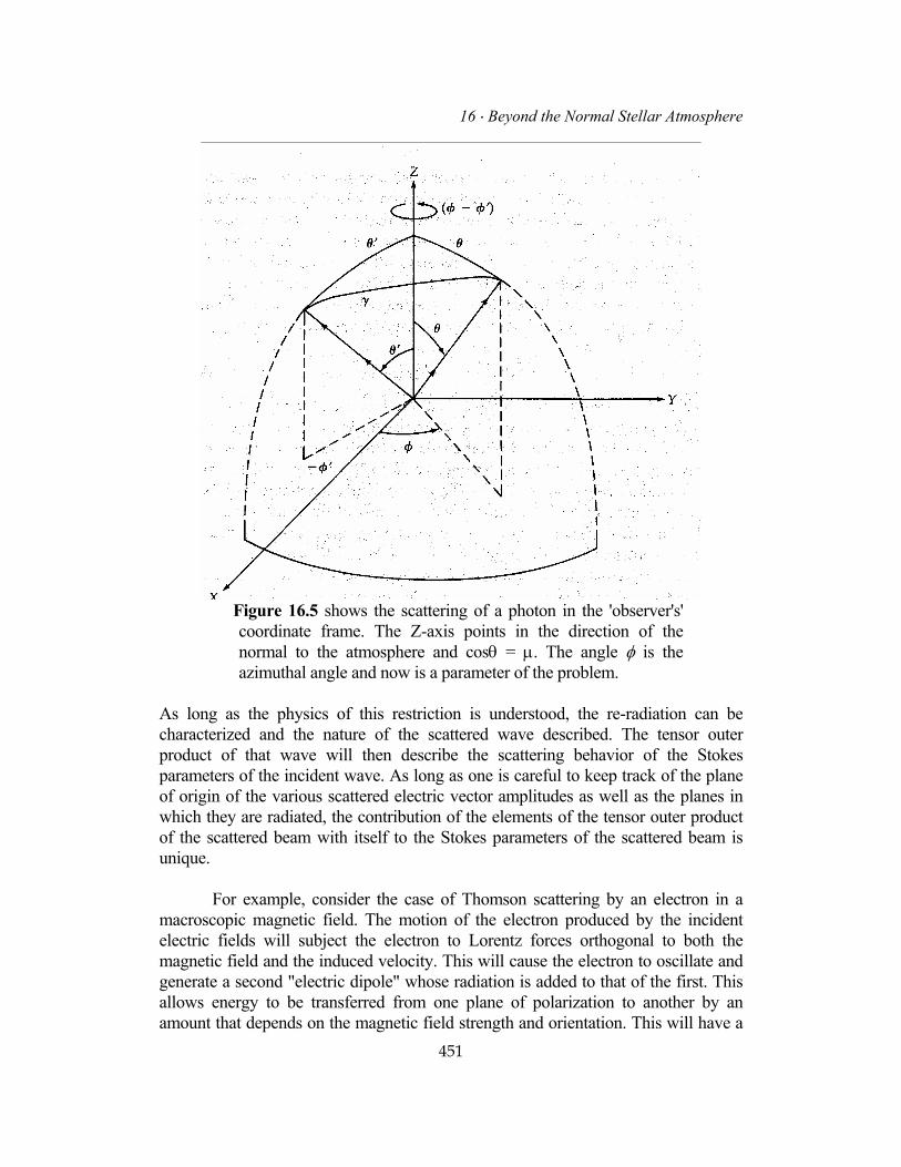
Figure 16.5 shows the scattering of a photon in the 'observer's'

coordinate frame. The Z-axis points in the direction of the normal to the atmosphere and cosθ = µ. The angle φ is the azimuthal angle and now is a parameter of the problem.

As long as the physics of this restriction is understood, the re-radiation can be characterized and the nature of the scattered wave described. The tensor outer product of that wave will then describe the scattering behavior of the Stokes parameters of the incident wave. As long as one is careful to keep track of the plane of origin of the various scattered electric vector amplitudes as well as the planes in which they are radiated, the contribution of the elements of the tensor outer product of the scattered beam with itself to the Stokes parameters of the scattered beam is unique. For example, consider the case of Thomson scattering by an electron in a macroscopic magnetic field. The motion of the electron produced by the incident electric fields will subject the electron to Lorentz forces orthogonal to both the magnetic field and the induced velocity. This will cause the electron to oscillate and generate a second "electric dipole" whose radiation is added to that of the first. This allows energy to be transferred from one plane of polarization to another by an amount that depends on the magnetic field strength and orientation. This will have a 451


profound effect on all the Stokes parameters. Contributions will be made to the scattered Stokes parameters from the interaction of the radiation by the initial electric dipole with itself, the interaction of that radiation with that of the magnetically induced dipole, and finally the self interaction of the magnetically induced dipole. If we represent the scattered electric fields as being composed of a component from the initially driven dipole E

r and the magnetically induced dipole M

r then we can write

the outer product of the scattered electric field with itself as

(16.2.22) Each of these tensor outer products will produce a scattering matrix, and the sum will represent the scattering of the Stokes parameters by electrons in the magnetic field. The first will be identical to the Rayleigh phase matrix, where each element has been reduced by an amount equal to the energy that has been fed into the magnetically induced dipole. The second matrix represents the mixing between the electric field of the initial dipole with that of the magnetically induced dipole. Since these dipoles radiate out of phase with one another by π/2, the information contained here will largely involve the U and V Stokes parameters. The last matrix represents the contribution from the magnetically induced dipole with itself and will depend strongly on the relative orientation of the magnetic field. Keeping track of the relative phases of the various components, we calculate the three scattering matrices to be

(16.2.23) where

(16.2.24)

452


The coordinates of the magnetic field with respect to the scattering plane of the incident photon are given by η and the polar angle ξ, respectively. The strength of the magnetic field is contained in the parameter x so that

(16.2.25) If we require that the scattering be conservative, then since energy is required to generate those oscillations, the amplitude of the incident electric vector will be reduced in order to supply the energy to excite them. However, the energy that excites the dipoles must be equal to the energy of the incident beam so that

(16.2.26) where ξ is the angle between the electric vector and the magnetic field. If we assume that the magnitude of the electric vector is reduced by ζ, then

(16.2.27) where

(16.2.28) r

If we assume that x<<1, then Er

will remain nearly parallel to E ' and we may expand equations (16.2.27), and (16.2.28) to give

(16.2.29) and we may write

(16.2.30) For zero magnetic field, one recovers the Rayleigh phase matrix. As the strength of the field increases, the contribution of the second two matrices increases and normal electron scattering decreases. As the gyro-frequency ωc is reached, the motion of the electron becomes circular and significant circular polarization is introduced to the beam along the direction of the magnetic field. Since we have ignored the resonance that occurs at the gyro-frequency (that is, x=1), these results are only approximate. For the scattering of natural light, r

[½I,½I,0,0], the strength of the components from the Rayleigh matrix are reduced while the R( M

rr) contributes solely to the V stokes parameter, indicating

that the beam will be circularly polarized when scattered along the magnetic field.

IE

453


This contribution diminishes as the scattering angle moves toward π/2. The contribution from the R( M

rr) matrix only has nonzero components that transfer

energy equally from IM

l to Ir and vice versa (for γ = π), but the contribution to Il vanishes as γ → π/2. The fact that U remains zero implies that the scattered radiation for γ = π/2 is linearly polarized with the plane of polarization perpendicular to the magnetic field. As one approaches the gyro-frequency, the transport of radiation becomes increasingly complex. Since the component of the electric field that is parallel to the magnetic field produces no Lorentz force on the electron, the interaction of the two orthogonal components of the generalized electromagnetic wave with the magnetic field are unequal. This anisotropic interaction has its optical counterparts in the phenomena known as Faraday rotation and a complex index of refraction. The phenomena enter the scattering problem as x2 so that our results are valid only for x << 1. At frequencies less that the gyrofrequency, the scattering situation becomes more complex as the entire energy of the photon may be absorbed by the electron in the form of circular motion. This energy may be lost through collisions before it can be reradiated. Again to utilize these matrices for problems involving radiative transfer requires that these matrices be transferred to the observer's frame. However, as they were developed primarily to indicate the method for generating the Stokes phase matrices, we will not develop them further. It seems clear that such techniques are capable of developing phase matrices for problems of considerable complexity. c Solution of the Equations of Radiative Transfer for Polarized

Light. While direct solution of the integrodifferential equations of radiative transfer may be accomplished by direct means, all the various rays characterizing the four Stokes parameters must be solved together so that the integrals required by the scattering part of the source function may be evaluated simultaneously. To obtain the necessary accuracy for low levels of polarization would require a computing power that would tax even the fastest computers. Even if the axial symmetry of the diffuse field can be used to advantage for some problems, cases involving incident radiation will require involving discrete streams in φ as well as θ. There is an approach involving the integral equations for the source function that greatly simplifies the problem. We have seen throughout the book 454


that the development of Schwarzschild-Milne equations for the source function always produced equations that involved moments of the radiation field, usually the mean intensity J. As long as the redistribution function can be expressed as a finite series involving tesseral harmonics of θ and φ, the source function can be expressed in terms of simple functions of θ and φ which multiply various moments of the radiation field that depend on depth only. As we did in Chapter 9, it will then be possible to generate Schwarzschild-Milne-like equations for these moments that depend on depth only. Indeed, since a moment of a radiation field cannot depend on angle, by definition, this effectively separates the angular dependence of the radiation field from the depth dependence. This is true even for the case of incident radiation. The solution of these equations will then yield the source function at all depths which, together with the classical solution for the equation of transfer, will provide a complete description of the radiation field in all four Stokes parameters. This conceptually simple approach becomes rather algebraically complicated in practice, even for the relatively simple case of Rayleigh scattering. The general case of this problem has been worked out by Collins11 and more succinctly by Collins and Buerger12 and we will only quote the results. The source functions for nongray Rayleigh scattering can be written as

(16.2.31) where the moments of the radiation field X(τ), Y(τ), Z(τ), M(τ), P(τ), and W(τ) depend on depth alone and satisfy these integral equations:

455


(16.2.32) The Λn operator is the same as that defined in Chapter 10 [see equation (10.1.16)] and produces exponential integrals of order n. The constants CN(τ) depend on the incident radiation field only and are attenuated by the appropriate optical path. It is assumed that the incident radiation encounters the atmosphere along a path defined by φ = 0. The values of these constants for plane-parallel polarized radiation are

(16.2.33) The parameters ξ and ζ also depend on the incident radiation alone and are given by

(16.2.34) These parameters basically represent the direct contribution to the source function from the incident radiation field. If the incident radiation is unpolarized, they are both zero. Note that only the first two integral equations for the moments X(τ) and Y(τ) are coupled and therefore must be solved simultaneously. In addition, the net radiative flux flowing through the atmosphere involves only these moments, so that only these two equations must be solved to satisfy radiative equilibrium. This can be shown by substituting the equations for the source functions into the definition for the radiative flux and obtaining

456


(16.2.35) or in differential form

(16.2.36) These two expressions are all that is needed to apply the Avrett-Krook perturbation scheme for constructing a model atmosphere. The remaining equations need to be solved only when complete convergence of the atmosphere has been achieved, and then only if the state of polarization for the emergent radiation field is required. d Approximate Formulas for the Degree of Emergent Polarization The complexity of equations (16.2.31) and (16.2.32) show that the complete solution of the problem of the transfer of polarized radiation is quite formidable. Clearly approximations that yielded the degree of polarization and its wavelength dependence would be useful. To get such approximation formulas, we plan to formulate them from the Stokes parameters I[I,Q,U,V] rather than I[Il,Ir,U,V] since the degree of polarization is just Q/I. We may generate the appropriate scattering matrix from equation (16.2.19) from the relation for the Stokes parameters I[I,Q,U,V] and I[Il,Ir,U,V] given in equation 16.2.7. The resulting matrix for the Stokes Scattering matrix is then

(16.2.37) Here we have replaced the notation of Chandrasekhar with

(16.2.38) To obtain the source function for Thomson-Rayleigh scattering we must carry out the operations implied by equation (16.2.21) for the source function. However, now we are to do it for all four of the Stokes parameters. This means that

457


we shall integrate all elements of the scattering matrix over φ' and θ'. However, we know that the geometry of the plane parallel atmosphere means that the solution can have no φ-dependence so that all odd functions of φ' must vanish as well as sin2φ'. Similarly the resulting source function can have no explicit φ-dependence. Also the elements of R[I,Q,U,V] contain a limited number of squares and products of the gijs. If we simply average these quantities over φ' we get

(16.2.39) Integration of these terms over θ' will then yield familiar moments of the Stokes parameters such as J and K (Section 9.3). If we let the subscript P stand for the different Stokes parameters, then expressing the product of the gijs in equation (16.2.39) and the Stokes vector in terms of the moments of the Stokes parameters yields

(16.2.40) Substituting these average values into the respective elements of equation (16.2.19) we can calculate the scattering fraction of the source functions for the Stokes parameters. Adding the contribution to the I-source function from thermal emission we can then write the source functions for all the Stokes parameters as

458


(16.2.41) where as before

(16.2.42) For an isotropic radiation field such as one could expect deep in the star that JI = 3KI and JQ = KQ = 0 since there is no preferred plane in which to measure Q. Under these conditions all fluxes vanish and the source functions become

(16.2.43) which is the expected result for isotropic scattering and is consistent with an isotropic radiation field. For anisotropic scattering the source function is no longer independent of θ. However, the θ-dependent terms depend on a collection of moments that measure the departure of the radiation field from isotropy. For a one dimensional beam JQ = KQ, while for an isotropic radiation field JI = 3KI. This is true for both SI and SQ. Indeed, the coefficient of the angular term is the same for both source functions. The fact that SU is zero means that U is zero throughout the atmosphere. This result is not surprising as for U to be non-zero would imply that polarization would have to have a maximum in some plane other than that containing the normal to the atmosphere and the observer (or one perpendicular to it). From symmetry, there can be no such plane and hence U must be zero everywhere. We are now in a position to generate integral equations for quantities that will explicitly determine the variation of the source functions with depth. Approximation of SQ in the Upper Atmosphere To begin our analysis of the polarization to be expected from a stellar atmosphere, let us consider the complete source functions for such an atmosphere. These can be written as

459


(16.2.44) where

(16.2.45) Let us first consider the pure scattering gray case so that 0)( =τε νν . Our problem then basically reduces to finding an approximation for Y(τν). For this part of the discussion, we shall drop the subscript n as radiative equilibrium guarantees constant flux at all frequencies. The quantity (JI-3KI ) occurs in Y(τ) and normally is the dominant term. However, in the Eddington approximation, this term would be zero. This clearly demonstrates that polarization is a 'second-order' effect and will rely on the departure of the radiation field from isotropy for its existence. The entire problem of estimating the polarization then boils down to estimating (J-3K) or the Eddington factor. The Eddington factor was defined in equation (10.4.9) and is a measure of the extent to which the radiation field departs from isotropy. If the radiation field is isotropic then f(τ)=1/3. If the radiation field is strongly forward directed then f(τ)=1. If the radiation field is somewhat flattened with respect to the forward direction then f(τ) can fall below 1/3. Thus we may write the source function for Q as

(16.2.46) It is fairly easy to show that if JI(τ), is given by the gray atmosphere solution

(16.2.47) where q(τ) is the Hopf function, that

(16.2.48) To obtain this result we have simply taken moments of the Q-equation of transfer, assumed fQ(τ) = 1/3, and used the Chandrasekhar n=1 approximation for q(τ). Thus k1 is the n=1 eigenvalue for the gray equation of transfer (see Table 10.1) and α2=3/2. C1 and C2 have opposite signs. Thus JQ(τ) will indeed vanish rapidly with optical depth. This rapid decline will also extend to SQ(τ). Thus we will assume that

460


(16.2.49) This means that

(16.2.50) This may be substituted back into equation (16.2.46) to yield

(16.2.51) Approximate Formulas for the Degree of Polarization in a Gray Atmosphere Since we can expect the maximum value of the polarization to occur at the limb (that is, θ = π/2), both Q(0,0) and I(0,0) will be given by the value of their source functions at the surface. If for I(0,0) we take that to be JI(0), we get for the degree of polarization to be

(16.2.52) Just as we calculated JQ(0) in equation (16.2.50) so we can calculate KQ(0) and determine fQ(0) = 1/5. Using the best value for fI(0) of 0.4102 [i.e., the 'exact-approximation' of Chandrasekhar], we get that the limb polarization for a gray atmosphere should be 12.35 percent. This is to be compared with Chandrasekhar's (1960) value of 11.713 percent. The accuracy of this result basically stems from the fact that the limb values only require knowledge of the surface values of fI and fQ so our approximations will give the best values at the limb. While the µ-dependence given by equation (16.2.52) will be approximately correct, we can hardly expect it to be accurate. The solution for µ>0 requires integrating the source function over a range of µτ which means that we will have to know the source function as a function of τ. Physically this amounts to including the limb-darkening in the expressions for I(0,µ) and Q(0,µ). Using expressions for the source functions obtained from the same kind of analysis that was used to get JQ(τ), we get a significant difference in the limb-darkening for I and Q. The increase of the source function for I with depth produces a decrease of the intensity at the limb. The limb is simply a less bright region than the center of the disk. However, the source function for Q declines rapidly as one enters the star so that the region of the star that is the 'brightest' in Q is the limb. Hence Q will suffer 'limb-brightening'. The ratio of these two effects will cause the polarization to drop much faster than (1-µ2) as one approaches the center of the disk from the limb. Determining the source functions τ-dependence in the same level of approximation that was used to get JQ(τ) yields

461


(16.2.53) or substituting in values of the constants for the same order of approximation we get

(16.2.54) The value of the polarization for µ=½ from equation (16.2.52) is P1(µ=.5) = 9.26 percent. In contrast, the value given by equation (16.2.54) is P2(µ=0.5) = 4.1 percent. This is to be compared with Chandrasekhar's value of 2.252 percent. Thus the limb-darkening is important in determining the center-limb variation of the polarization and it drops much faster than would be anticipated from the simple surface approximation. The Wavelength Dependence of Polarization The gray atmosphere, being frequency independent, tells us little about the way in which the polarization can be expected to vary with wavelength. However, it is clear from the approximation formulae for the center-limb variation of the gray polarization, that the polarization is largely determined by the quantity [1-3fI(0)]. This quantity basically measures the departure from isotropy of the radiation field. In any stellar atmosphere, this will be determined by the gradient of the source function. Since the polarization is largely determined by the atmosphere structure above optical depth unity, we may approximate the source function by a surface term and a gradient so that

(16.2.55) Thus,

(16.2.56) This enables us to write the term that measures the isotropy of the radiation field as

(16.2.57) Thus replacing the term that measures the anisotropy of the radiation field with b yields

(16.2.58) 462


If for purposes of determining the wavelength dependence of the polarization, we take the source function to be the Planck function, then the normalized gradient bν becomes

(16.2.59) The frequency ν0 is the reference frequency at which the temperature gradient is to be evaluated. In this manner, the temperature gradient is the same for all frequencies and the frequency dependence is then determined by the derivative of the Planck function and the term dτ0/dτν. This term is simply the ratio of the extinction coefficients at the reference frequency and the frequency of interest. It is this term that is largely responsible for the frequency dependence of the polarization in hot stars. If for purposes of approximation we continue to use the Planck function as the source function, we can evaluate much of the expression for bν explicitly so that

(16.2.60) where

(16.2.61) We can write the polarization as

(16.2.62) It is clear that for the gray atmosphere εν = ε0 = 0, and the maximum polarization will be achieved where βν is a maximum. By letting α = (hν/kT), setting Pν(0) equal to the gray atmosphere result, and using the gray atmosphere temperature distribution, we find that the gray result will occur near α = 4. This lies between the maximum of Bν (α = 2.82) and Bλ (α = 4.97) and is virtually identical to the frequency at which νBν (α = 3.92) is a maximum which is practically the same as the frequency for which [dBν/dT] (α = 3.83) is a maximum. Thus, to the accuracy of the approximation, the gray polarization will occur at the frequency for which the source function gradient is a maximum. This results from the fact that Q will attain its largest value when JI -3KI is a maximum. This will occur when the source function gradient is a maximum which, since the radiative flux is driven by that gradient, is also the energy maximum. For larger values of the frequency fI(0) will become larger meaning that the degree of polarization can exceed the gray value, but the magnitude of Qν will decrease.

463


In the non-gray case, the situation is somewhat more complicated. Here, in addition to the frequency dependence of the source function gradient, the variation of the opacity with frequency strongly influences the value of the polarization. If we assume that the gray result is actually realized for hot stars in the vicinity of the energy maximum, then the polarization in the visible will be roughly given by

(16.2.63) That is, it will drop quadratically with (1-εν) as one moves into the visible. The change in εν with frequency will be largely by the change in κν. To the extent that this is largely due to Hydrogen, we can expect the opacity to vary as ν-3. Thus, in stars where the dominant extinction is from absorption by hydrogen and the energy maximum is in the far ultraviolet, we can expect the polarization to drop by several powers of ten from its maximum value. In stars where electron scattering is the dominant opacity source, a significant decrease in the degree of polarization will still in the visible as a result of the increase in the pure absorption component of the extinction. In the limit of α = (hν/kT) << 1, the source function asymptotically approaches a constant given by the temperature gradient, and the wavelength dependence of the polarization depends only on the opacity effects. In the case where α>>1, β is proportional to α times the normalized temperature gradient and the polarization will continue to rise into the ultraviolet until there is a change in the opacity. Thus we should expect the early type stars to show significant polarization approaching or exceeding the gray value in the vicinity of the Lyman Jump. Little polarization will be in evidence in the Lyman continuum as a result of the marked increase in the absorptive opacity. The polarization will also decline as one moves into the optical part of the spectrum to values typically of the order of 0.01 percent at the limb and will slowly decline throughout the Paschen continuum. Everything done so far has presupposed that the dependence of the source function near the surface can be expressed in terms of a first-order Taylor series. In many stars, this is not adequate as there is a very steep plunge in the temperature near the surface. This will require a substantial second derivative of opposite sign from the first derivative to adequately describe the surface behavior of the source function. It is clear from equations (16.2.55) and (16.2.56) that the presence of such a term will increase the value of (JI -3KI) and could in principle reverse its sign resulting in a positive degree of polarization (i.e., polarization with the maximum electric vector aligned with the atmospheric normal). Detailed models of gray atmospheres indeed show this and it can be expected any time the second order limb-darkening coefficient to positive and greater than half the magnitude of the first order limb-darkening coefficient.

464


e Implications of the Transfer of Polarization for Stellar

Atmospheres. It is clear from equations (16.2.33) that in the absence of illumination on the atmosphere, all the CN's in the integral equations for the moments [equations (16.2.32)] vanish and all but the first two integral equations become homogeneous. The last two of equations (16.2.18) deal with the propagation of the ellipticity of the polarization, and they make it clear that in the absence of incident elliptically polarized light and sources of such light in the atmosphere, Rayleigh scattering will make no contribution to the Stokes parameter V. The trivial solution V = 0 will prevail throughout the atmosphere, and no amount of circularly polarized light is to be expected. In the absence of incident radiation, the resulting homogeneity of the integral equations for Z(τ) and M(τ) simply means that it is always possible to choose a coordinate system aligned with the plane of the resulting linear polarization so that U = 0 is also true throughout the atmosphere. The only parameter that prevents the integral equations for X(τ) and Y(τ) from becoming homogeneous is the presence of the Planck function tying the radiation field of the gas to the thermal field of the particles. Interpretation of the Polarization Moments of Radiation Field From the behavior of the integral equations (16.2.32), it is possible to understand the properties of the Stokes parameters that they represent. For numerical reasons, the scattering fraction 1-ε(τ) has been absorbed into the definition of the moments. Clearly W(τ) and P(τ) describe the propagation of the Stokes parameter V throughout the atmosphere. Since both U and V are basically geometric, two equations are required to determine the magnitude and quadrant of the angular parameters which they contain. Since the scattering matrix [equation (16.2.19)] is reducible with respect to V (i.e., only the diagonal element describing scatterings from V' into V is nonzero), it is not surprising that these two equations stand alone and can generally be ignored. The two equations for Z(τ) and M(τ) describe the orientation of the plane of linear polarization throughout the atmosphere. Since the orientation of the plane of polarization is also a geometric quantity, no energy is involved in the propagation of Z(τ) and M(τ) so their absence in the equations for radiative equilibrium is explained. The moments X(τ) and Y(τ) describe the actual flow of the energy field associated with the photons. An inspection of the X(τ) equation of equations (16.2.32) shows that X(τ) is very like the mean intensity J. The moment Y(τ) measures the difference between Il and Ir and therefore describes the propagation of the degree of linear polarization in the atmosphere. Since both these moments appear in the flux equations, the amount of linear polarization does affect the condition of radiative equilibrium and hence the atmospheric structure. However, in the stellar atmosphere, the effect is not large.

465


The reason that there should be any effect at all can be found in the explanation for the existence of scattering lines in stars. Anisotropic scattering redirects the flow of photons from that which would be expected for isotropic scattering. This redirection increases the distance that a photon must travel to escape the atmosphere, thereby increasing the probability that the photon will be absorbed. This effectively increases the extinction coefficient and the opacity of the gas. While the effect is small for Rayleigh scattering, it has been found to play a significant role in the stellar interior when electron scattering is a major source of the opacity. In the stellar atmosphere, the effect on the stellar structure is small because the photon mean free path is comparable to the dimensions of the atmosphere (by definition), so that there is simply not enough space for anisotropic scattering to significantly affect the photon flow. However, Rayleigh scattering will always produce linear polarization of the emergent radiation field. Since the Rayleigh phase function correctly describes electron scattering as resonance scattering, we can expect that polarization will be ubiquitous in stellar spectra, even in the absence of incident radiation. Effects on the Continuum The early work by Chandrasekhar8,9 on the gray atmosphere showed that one might expect up to 11 percent linear polarization at the limb of a star with a pure scattering atmosphere. As was pointed out earlier, even this rather large polarization would average to zero for observers viewing spherical stars. Hence, Chandrasekhar suggested that the effect be searched for in eclipsing binary systems. Such search led Hiltner13 and Hall14 to independently discover the interstellar polarization. It was not until 1984 that Kemp and colleagues15 verified the existence of the effect in binary systems. However, the measured result was significantly smaller than that anticipated by the gray atmosphere study. The reason can be found by considering the effects that tend to destroy intrinsic stellar polarization. The most significant is the near-axial symmetry about the line of sight of most stars. This tends to average any locally generated polarization to much lower values. The second reason results from the sources of the polarization itself. It is obvious that to generate polarization locally on the surface of a star, it is necessary to have opacity sources that produce polarization. In the hot early-type stars (earlier than B3), electron scattering is the dominant source of opacity, while in the late-type stars Rayleigh scattering from molecules is a major source of continuous opacity. Unfortunately, the spectra of these stars are so blanketed by atomic and molecular lines that it is difficult to find a region of the spectrum dominated by the continuous opacity alone. For stars of spectral type between late B and early K, there is a general lack of anisotropic scatterers making a major contribution to the total opacity, so that polarization is generally absent even locally.

466


In the early-type stars where anisotropic scattering electrons are abundant, the third reason comes into play and is basically a radiative transfer effect. To understand this rather more subtle effect, consider the following extreme and admittedly contrived examples. Remember that an electron acting as an oscillating dipole will scatter photons which are polarized in a plane perpendicular to the scattering plane. Consider a region of the atmosphere so that the observer sees the last scattering and is therefore in the scattering plane. The distribution of polarized photons that the observer sees will then reflect the distribution of the photons incident on the electrons. Further consider a point near the limb so that photons emerging from deep in the atmosphere will be scattered through 90 degrees and be 100 percent linearly polarized. If the source function gradient is steep, most of the photons scattered toward the observer will indeed come from deep in the atmosphere and exhibit such polarization and the observer will see a beam of light, strongly polarized in a plane tangent to the limb. However, if the source function gradient is shallow or nearly nonexistent, the majority of last scattered photons will originate not from deep within the star, but from positions near the limb. There will then be a surplus of scattered photons, with their scattering plane parallel to the limb and therefore polarized at right angles to the limb. Somewhere between these two extremes there exists a source function gradient which will produce zero net polarization locally at the limb. This argument can be generalized for any point on the surface of the star. Unfortunately, in the early-type stars that abound with anisotropically scattering electrons, the energy maximum lies far in the ultraviolet part of the spectrum. Thus the source function in the optical part of the spectrum is weakly dependent on the temperature and hence has a rather flat gradient. So these stars may exhibit little more than one percent or so of linear polarization in the optical part of the spectrum, even at the limb. The integrated effect, even from a highly distorted star, is minuscule. Such would not be the case for the late-type stars where the energy maximum lies to longer wavelengths than the visible light. These stars have very strong source function gradients in the visible part of the spectrum and should produce large amounts of polarization of the local continuum flux. There remains a class of stars for which significant amounts of polarization may be found in the integrated light. These are the close binaries. Here the source of the polarization is not the star itself, but the scattered light of the companion. Although little has been done in a rigorous fashion to investigate these cases, Kuzma16 has found that measurable polarization should be detected in at least some of these stars. Study of these stars offers the significant advantage that the polarization will be phase dependent and so the effects of interstellar polarization may be removed in an unambiguous manner. Much work remains to be done in this area, but it must be done very carefully. All the effects that determine the degree of polarization of the emergent light depend critically on the temperature distribution of the upper atmosphere. Thus, such studies must include nongray and non-LTE effects. Kuzma16 also included the effect that the incident radiation comes not from a point

467


source, but from a finite solid angle and found that this significantly affected the result. While the task of modeling these stars is formidable, the return for determining the structure of the upper layers of the atmosphere will be great. Effects of Polarization on Spectral Lines While that a line formed in pure absorption will be completely unpolarized except for contributions from electron scattering, this is not the case for scattering lines. For resonance lines where an upward transition must be followed quickly by a downward transition, the reemission of the photon is not isotropic, but follows a phase function not unlike the Rayleigh phase function. The scattering process can change the state of polarization in much the same fashion as electron scattering does. Thus, these lines can behave in much the same way as electrons in introducing or modifying the polarization of a beam of light. Since any absorption has a finite probability of being followed immediately by the reemission of a similar photon, any spectral line has the possibility of introducing some polarization into the beam. For example, under normal atmospheric conditions, the formation of Hβ results in a scattered photon about 25 percent of the time. For Hα the fraction can approach 50 percent. In other strong lines such as the Fraunhofer H and K lines of calcium, the fraction is much larger. Thus one should not be surprised if large amounts of local polarization are present in such lines. Unfortunately, the effect will be wavelength dependent. The majority of the wavelength dependence arises from the redistribution function by linking one frequency within the line to another. The introduction of a frequency-dependent redistribution function greatly complicates the problem. To handle this problem, it is necessary to express the redistribution function in some analytic form such as those of Hummer (see Section 15.3). Furthermore, one cannot use the angle-averaged forms because the angle dependence is crucial to the transfer of polarized radiation. McKenna17 has developed the formalism from the standpoint of integral equations for the moments of the radiation field for a fairly general class of spectral lines. In the case of coherent scattering, these equations reduce to those presented here. For a general redistribution function, the equations are much more complicated. Using the corrected Hummer RIV for the case of the sun, McKenna18 found that weak resonance lines showed a slowly decreasing degree of polarization from the core to the wings. The structure of the line as well as the state of polarization agreed well with observation and reproduced the center-limb variation observed for such lines. For strong resonance lines, a sharp spike in the polarization at the line core was found that rapidly diminished as one moved away from the line core before rising again and then diminishing into the wings as, in the case of the weak lines. Again, this effect is seen in the sun and provides a useful diagnostic tool for the upper atmosphere structure.

468


In most stars, except those distorted by rotation, binary systems, and nonradially pulsating stars, symmetry will tend to destroy these effects. But for these other classes of stars, line polarization may provide a useful constraint on their shape and structure. Unfortunately, the correct redistribution function for hydrogen has yet to be worked out. Since the hydrogen lines are readily observed and are often found in situations where the geometry would indicate little symmetry, an analysis of this type extended to these lines would provide an interesting constraint on the physical nature of the system. 16.3 Extended Atmospheres and the Formation of Stellar Winds So far we have limited the subject of this book to the interiors and atmospheres of normal stars. However, we cannot leave the subject of stellar astrophysics without offering some comments about the transition between the outer layers of the stars and the interstellar medium that surrounds the stars. This is the domain where all of the simplifying assumptions, which made the description the inner regions of the star possible, fail. As one moves outward from the photosphere, through the chromosphere and beyond, he or she will encounter regions that involve some of the most difficult physics in astrophysics. Here the regions become sufficiently large that the plane-parallel assumption which so simplified radiative transfer is no longer valid, for the transition region may extend for many stellar radii. The density of matter is so low that LTE can no longer be applied to any elements of the gas. Because of the low density, the radiative interactions, while remaining crucial to the understanding of the structure of the medium, receive competition from previously neglected modes of energy transport. From observation, we know that turbulence is present in most stars. In some instances, the mechanical energy of the turbulent motion can be systematically transmitted to the outer layers of the star in amounts that compete with the energy from the radiation field. For some stars, the coupling of the magnetic field of the underlying star may provide a mechanism for the transmission of the rotational energy and momentum of the star to the surrounding low-density plasma. The influx of energy from all sources seems to be sufficient to cause much of the surrounding plasma to be driven into the interstellar medium. Thus, we must deal with a medium in which hydrostatic equilibrium no longer applies. Continuous absorption is no longer of great significance so that the primary coupling of the radiation field to the gas is through the bound-bound transitions that produce the line spectra of stars. However, as we have seen, the frequency dependence of the line absorption coefficient is quite large, so Doppler shifts supplied by the mass motions of the gas will yield an absorption coefficient that is strongly dependent on the location of the gas. Thus the coupling of the radiation field is further complicated. 469


The region surrounding the star where these processes take place is generally known as the extended atmosphere of the star while the material that is driven away is referred to as the stellar wind. It is likely that all stars possess such winds, but the magnitude of the mass loss produced by them may vary by 8 powers of 10 or more. The primary processes responsible for their origin differ greatly with the type of star. For example, the wind from the sun originates from the inability of the hot corona to come into equilibrium with the interstellar medium, so that the outer layers "boil" away. The details of the solar wind are complicated by coupling of the rotational energy of the sun to the corona through the solar magnetic field. Thus the outer regions of the solar atmosphere are accelerated outward at an average mass loss rate

of the order of 10-14M⊙ per year. The heating of the corona is likely to result from coupling with the convective envelope of the sun. Thus corona-like winds are unlikely to originate in the early-type stars that have radiative envelopes. For the hotter stars on the left-hand side of the H-R diagram, the acceleration mechanism is most likely radiative in origin. The coupling of the turbulent motions of the photosphere to the outer regions of the atmosphere is so poorly understood that its role is not at all clear. However, in the case of some giants and supergiants, this coupling may well be the dominant source of energy driving the stellar wind. In the face of these added difficulties, it would be both beyond the scope of this book and presumptuous to attempt a thorough discussion of this region. For that the reader is directed to the supplemental reading at the end of the chapter. We will merely outline some approaches to some aspects of these problems that have yielded a small measure of understanding of this transition region between the star and the surrounding interstellar space. a Interaction of the Radiation Field with the Stellar Wind For those stars where the stellar wind results from the star's own radiation, not only is the wind driven by the radiation, but also the motion of the material influences the radiative transport. Thus one has a highly nonlinear problem involving the formidable physics of hydrodynamics and radiative transfer. This interplay between the two is the source of the major problems in the theory of radiatively driven stellar winds. Since it is clear that we must abandon most of the assumptions in describing this region, we will have to replace them with others. Thus I shall assume that these outer regions are spherically symmetric. Although this is clearly not the case for many stars, an understanding of the problems posed by a spherically symmetric star will serve as a foundation for dealing with the more difficult problems of distorted stars. Since we have already dealt with the problems of spherical radiative transport (see Section 10.4) and departures from LTE (see Chapter 15), we concentrate on the

470


difficulties introduced by the velocity field of the outer atmosphere and wind. One of the earliest indications that some stars were undergoing mass loss came from the observation of the line profiles of the star P-Cygni. The Balmer lines (and others) in the spectrum of this star showed strong emission shifted slightly to the red of the stellar rest wavelength and modest absorption centered slightly to the blue side of the rest wavelength. This was recognized as the composite line profile arising from an expanding envelope with the emission being formed in a relatively transparent out- flowing spherical envelope. The "blue" absorption arose from that material that was moving, more or less, toward the observer and was seen silhouetted against the hotter underlying star (see Figure 16.6). Such line profiles are generally known as P-Cygni profiles and are seen during novae outbursts and in many other types of stars. To understand the formation of such profiles, one must deal with the radiative transport of spectral line radiation in a moving medium. If the envelope surrounding the star cannot be assumed to be optically thin to line radiation, then one is faced with a formidable radiative transfer problem. In 1958, V. V. Sobolev21 realized that the velocity gradient in such an expanding envelope could actually simplify the problem. If the gradient is sufficiently large, then the relative Doppler shifts implied by that gradient could effectively decouple line interaction in one part of the envelope from that in another part. Since the outflow velocities often reach several thousand kilometers per second, the region of the envelope where photons are not Doppler-shifted by more than the line width can actually be quite thin. The contribution to the observed line profile at any given frequency therefore arises from emission (or absorption) occurring on surfaces of constant radial (i.e., line-of-sight) velocity. The extent of that contribution will then depend on the probability that a photon emitted on one of these surfaces can escape to the observer.

471


Figure 16.6 depicts the expanding envelope of a star and the regions

that give rise to the corresponding P-Cygni profile.

Consider an envelope which is optically thick to line radiation surrounding a stellar core of radius rc whose continuum radiation passes freely through the envelope. Let us further assume that the line is such that complete redistribution is an appropriate choice for the redistribution function. Finally, we define β to be the probability that an emitted photon will escape from the envelope. Clearly such a probability will depend on the line width and the velocity gradient. We can then write the local value for the average mean intensity in the line as

(16.3.1)

472

where (1-β)S(r) is the contribution to the local radiation field from those photons created in the line that did not escape and βcIc represents those continuum photons that have penetrated to that part of the envelope.


An estimate of β and βc will then provide us with a relationship between J and S which we can substitute into equations for the non-LTE source function developed in Chapter 15 [see equations (15.2.19) and (15.2.25)]. The mean escape probabilities β and βc will depend on local conditions only if the velocity gradient is sufficiently large that the conditions determining the probabilities can be represented by the local values of temperature and density. Castor20 has developed this formalism for a two-level atom and it is nicely described in Mihalas21. Basically, the problem becomes one of geometry. Contributions to the local mean intensity will come largely from surfaces within the envelope which exhibit a relative Doppler shift that is less than the Doppler width of the line. Castor finds this to be

(16.3.2) where

(16.3.3) is simply the velocity measured in units of the thermal velocity characterizing the line width and

(16.3.4) which occurs from expanding the effective optical path in a power series of the velocity field and retaining only the first-order term. The parameter τ0 is effectively the optical depth in the line along a radius from the star and is defined by

(16.3.5) This quantity is essentially the line extinction coefficient multiplied by some effective length that is obtained by dividing by the dimensionless velocity gradient. We may approximate βc by the following argument. Since βc is essentially an escape probability of a continuum photon leaving the envelope by traveling in any direction, it is essentially the same as β except for the probability of the photon's hitting the stellar core. That probability is given simply by the fraction of 4π occupied by the core itself and is commonly called the dilution factor since it is the amount by which the local radiation density is diluted as one recedes from the star. The dilution factor W is therefore

473


(16.3.6) so that

(16.3.7) We now have β and βc defined in terms of the velocity field, position, and parameters of the gaseous envelope that determine the local effective optical depth in the line τ0. Remembering that

(16.3.8) we may substitute into either of the non-LTE source functions given by equation (15.2.19) or (15.2.25) and obtain the source function for the line. Once the line source function is known, the solution for the equation of transfer (see Section 10.4 for spherical geometry) can be solved and the line profile obtained. Solution of this problem also yields the radiant energy deposited in the envelope as a result of the line interactions. By doing this for a number of lines, the local effects of radiation on the envelope can be determined. This is one of the primary factors in determining the dynamics of the envelope. b Flow of Radiation and the Stellar Wind Most progress in understanding stellar winds has been made with the radiation-driven winds of the early-type stars. While coronal winds of the later-type stars are important, particularly for slowing down the rotational velocity of these stars by magnetic breaking, the uncertainties concerning the formation of their coronal source force us to leave their discussion another to elucidate. What is presently known about them is nicely summarized by Mihalas21(pp.521-540) and Cassinelli22. Instead, we concentrate on some aspects of the large winds encountered in the early-type stars. In Chapter 6 [equation (6.5.2)] we showed that if the radiation pressure became sufficiently high, a star would become unstable. While many stars on the upper main sequence approach this limit, they still fall short. Yet these same stars exhibit significant mass loss in the form of a substantial stellar wind. In 1970, Leon Lucy and Philip Solomon23 showed that, under certain circumstances, the coupling of the radiation field to the matter in the upper atmosphere through the strong resonance lines of certain elements could provide sufficient momentum transport to the envelope to drive it away from the star. This idea was developed more fully by 474


Castor, Abbot, and Klein24 to provide the foundations for the theory of radiatively driven stellar winds. Castor, Abbot, and Klein found that by including the effects of the large number of weaker lines present in material of the high atmosphere, accelerations 100 times greater than those found by Lucy and Solomon would result. This implied that mass loss from radiatively driven winds could be expected in cooler stars with higher surface gravities than the supergiants considered by Lucy and Solomon. Thus, stellar winds should be a ubiquitous phenomenon throughout the early-type stars. The basic approach to describing any phenomenon of this type is to write down the conservation laws that must apply. To make the description as simple as possible, we assume that the flow is steady. Again, we assume spherical symmetry and remind the reader that the relevant conservation laws all have their origin in the Boltzmann transport equation developed in Chapter 1. Mass will be continuously lost by the wind, but for a steady flow, the mass flux through a spherical shell of radius r will be constant and given by

(16.3.9) The conservation of momentum requires

(16.3.10) where gr is the radiative acceleration. The conservation of energy and thermodynamics can be expressed by

(16.3.11) r

where U is the internal energy of the gas and tF is the total energy flux whose divergence can be described in terms of the energies QA, QR, and QC deposited locally in the gas by acoustical, radiative, and conductive processes respectively. Since both the radiative and gravitational accelerations vary as r -2, it is common to introduce the parameter

(16.3.12) If the wind is assumed to be radiatively driven, then QA = 0. Similarly the material density is sufficiently low that QC = 0. If the total energy in the flow is significantly less than the stellar luminosity, we may assume that radiative equilibrium may be locally applied, so that

475


(16.3.13) which greatly simplifies the energy equation. The energy and momentum equations can now be combined to yield

(16.3.14) which, after the total energy of the gas is defined to be

(16.3.15) can be integrated to give

(16.3.16) Thus even if the total energy of the gas near the star is negative, continual radiative acceleration can introduce sufficient energy to drive the energy positive and thus allow it to escape. As an example, consider the case where the gas in the wind is isothermal so that we can introduce an equation of state of the form

(16.3.17) where the speed of sound cs is constant. We can then differentiate equation 16.3.9 and eliminate dP/dr from equation (16.3.10) to get

(16.3.18) For supersonic flow to occur, the numerator of the right hand side of equation (16.3.18) must vanish at the point the speed of sound is reached (that is, v = cs). This places significant constraints on the value that Γ must have at the transonic point. Cassinelli 22 shows that this requires additional radiative heating of the gas as it approaches the transonic point. He suggests that scattering by electrons and resonance lines can do the work required to meet the conditions at the transonic point. Beyond the transonic point, further acceleration is most likely driven by the line opacity.

476


Since it has been shown that it is possible to drive stellar winds radiatively for stars whose luminosity is well below the Eddington luminosity, it remains for a complete and fully consistent model to be made. The problem here is largely numerical for the basic physical constraints are understood. To be sure these problems are formidable. Correct representation of the radiative acceleration requires calculation of the effects due to the myriads of weak spectral lines that populate the ultraviolet region of the spectrum where these stars radiate most of their energy. The energy balance equations must be solved to properly incorporate the effects of heating near the transonic point and to determine the temperature structure of the flow. Then the hydrodynamic flow equations will have to be solved numerically, incorporating an appropriate equation of state. Of course, all this must be done in non-LTE so that the proper ionization and excitation structure can be obtained. Undoubtedly the Castor, Abbot, and Klein models have pointed the correct way to understanding radiatively driven winds, but much remains to be done before the models can be used as a probe of the physics of the outer layers of stars. This brief look at the problems of extended atmospheres and radiatively driven winds points out that the transition region between the normal stellar atmosphere and the interstellar medium is a difficult region to understand. A closer look at the chromospheres and coronas of other stars would have shown the same, or possibly more difficult, problems. Certainly the description of the transition zone for nonspherical stars will include more difficulties and require greater cleverness on the part of astrophysicists to understand them. Certainly this will be necessary if we are to understand the evolution of close binary stars in sufficient detail to understand their ultimate fate and the manner in which they influence the interstellar medium. Without that understanding, the evolution of the galaxy will be difficult, if not impossible, to understand. And without a reliable knowledge of galactic evolution can we ever hope to delineate the evolution, of the universe as a whole? Problems 1. Show that equation (16.1.4) is indeed an equation for the diffuse field source

function for an illuminated atmosphere. 2. Show that equations (16.1.8), and (16.1.9) do give the correct form of the

Avrett-Krook perturbation scheme for an illuminated stellar atmosphere. 3 Find an integral expression for the radiative flux transmitted horizontally

through a plane-parallel stellar atmosphere that is illuminated by a point source located at [µ0=cos θ0, φ0=0].

477


4. Show how the degree of polarization P defined by equation (16.2.6) changes with a rotation of the observer's plane of observation.

5. Show that the group properties assigned to the rotation matrix L(φ) [defined

in equation (16.2.9)] are indeed those given in equation (16.2.10). 6. Show that equation (16.2.33) follows from the definition of the radiative flux

and the moments of the polarized radiation field. Derive an analogous expression for the horizontal flux transported through a plane-parallel atmosphere under the conditions specified in Problem 3, assuming that the incident radiation is unpolarized.

7. Show that equation (16.3.18) is a solution to the more general equations of

motion given by equation (16.3.10) in the case of an isothermal atmosphere. References and Supplemental Reading 1. Chandrasekhar, S.Radiative Transfer, Dover, New York, 1960, p. 22. 2. Buerger, P.F Illuminated Stellar Atmospheres, Ap.J. 177, 1972, pp. 657 -

664. 3. Karp, A.H."A Modification of the Avrett-Krook Temperature-Correction Procedure", Ap.J. 173, 1972, pp. 649 - 652. 4. Anderson, L., and Shu, F.H. On the Light Curves of W Ursae Majoris Stars, Ap. J. 214, 1977, pp. 798 - 808. 5. Milne, E.A. ”Thermodynamics of Stars", Handbuch der Astrophysik, vol. 3, (first half), Springer-Verlag, Berlin, 1930, pp. 134 - 141. 6. Kuzma, T.J.: On Some Aspects of the Radiative Interaction in a Close Binary System, doctoral thesis, The Ohio State University, Columbus, 1981. 7. Stokes, G.G. On the Composition and Resolution of Streams of Polarized Light from Different Sources, Trans. Cam. Phil. Soc. 9, 1852, pp. 399 - 416. 8. Chandrasekhar, S. On the Radiative Equilibrium of a Stellar Atmosphere X, Ap.J.103, 1946, pp. 351 - 370. 9. Chandrasekhar, S. On the Radiative Equilibrium of a Stellar Atmosphere XI, Ap.J.104, 1946, pp. 110 - 132. 478


10. Code, A.: Radiative Equilibrium in an Atmosphere in which Pure Scattering and Pure Absorption Play a Role, Ap.J. 112, 1950, pp. 22 - 47. 11. Collins, G.W.,II: Transfer of Polarized Radiation, Ap.J. 175, 1972, pp. 147 - 156. 12. Collins, G.W.,II, and Buerger, P.F. "Polarization from Illuminated Non-Gray Stellar Atmospheres", Planets, Stars, and Nebulae Studied with Photopolarimetry, (Ed: T. Geherels), University of Arizona Press, Tucson, 1974, pp. 663 - 675. 13. Hiltner, W.A.: Polarization of the Light from Distant Stars by Interstellar

Medium, Science 109, 1949, p.165. 14. Hall, J.S.: Observations of the Polarized Light from Stars, Science 109, 1949, pp. 166 - 167. 15. Kemp, J.C., Henson, G.D., Barbour, M.S., Krause, D.J., and Collins, G.W.,II

Discovery of Eclipse Polarization in Algol, Ap.J., 273, 1982, pp. L85 - L88. 16. Kuzma, T.J.: On Some Aspects of the Radiative Interaction in a Close Binary

System, doctoral thesis, The Ohio State University, Columbus, 1981, p. 135. 17. Mc Kenna, S. The Transfer of Polarized Radiation in Spectral Lines: Formalism and Solutions in Simple Cases, Astrophy. & Sp. Sci. 108, 1985, pp. 31 - 66. 18. McKenna, S. The Transfer of Polarized Radiation in Spectral Lines: Solar-Type Stellar Atmospheres, Astrophy. & Sp. Sci. 106, 1984, pp. 283 - 297. 19. Sobolev, V.V.: The Formation of Emission Lines, Theoretical Astrophysics, (Ed: V.A. Ambartsumyan, Trans. J.B.Sykes), Pergammon, New York, 1958, pp. 478 - 497. 20. Castor, J.I.: Spectral Line Formation in Wolf-Rayet Envelopes, Mon. Not. R. astr. Soc. 149, 1970, pp. 111 - 127. 21. Mihalas, D.: Stellar Atmospheres, 2d ed., W. H. Freeman, San Francisco, 1978, pp. 478 - 485.

479


22. Cassinelli, J.P. "Stellar Winds", Annual Reviews of Astronomy and

Astrophysics, (Ed.: G.Burbidge), vol. 17, Annual Reviews, Palo Alto, Calif., 1979, pp. 300 - 306.

23. Lucy, L.B., and Solomon, P.M. Mass Loss by Hot Stars , Ap.J. 159, 1970, pp. 879 - 893. 24. Castor, J.I., Abbot, D.C., and Klein, R.I. Radiation Driven Winds in Of Stars, Ap. J. 195, 1975, pp. 157 - 174. For general review on the subject of stellar winds one should read Cassinelli22 pp. 275-308.

Epilogue

. . . Those who have labored through this entire book will have noticed that the first half appears to form a more cohesive and understandable unit than the second half. The pedagogy seems more complete for the theory of stellar interiors than for stellar atmospheres. I believe this to be an intrinsic property of the material rather than a reflection of the my ability. More effort and minds have been involved in the formulation of the theory of stellar interiors and evolution than in the development of the theory of stellar atmospheres. More importantly, more time has elapsed during which the central ideas, important concepts, and their interrelationships can become apparent. This distillation process requires time as well as good minds to produce the final product. The reason this is not simply a temporal accident, but has its origin in the relative difficulty of the formulation of the subjects themselves. I have emphasized throughout this book the steady removal of simplifying assumptions as the description of stellar structure moves progressively out from the center of the star to the surface and beyond. This loss of assumptions that make the physical description of the star easier to effect also sets the time scale for the development of the subject itself, for people generally try to solve the simple problems first. So the effort to understand the stellar interior began in earnest as soon as nuclear physics delineated 480


the source of the energy in stars. This is not to belittle the elegant work with polytropes that began at the end of the nineteenth century. But it is clear that fully credible models of stellar interiors, suitable for the description of stellar evolution, could not be made without certain knowledge of the origin of a star's source of energy. After the elucidation by Hans Bethe of the probable energy sources for the sun, the theory of stellar structure and evolution developed with remarkable speed. In a mere two decades, one of which was dominated by world war II, the basic framework of the theory of stellar evolution was in place. Although the origin of stellar atmospheres can be traced back nearly as far as that of stellar interiors, its development has been slower. It is tempting to suggest that the theory required the existence of good stellar interior models before it could be developed, but that would be false. The defining parameters for the stellar atmosphere are known sufficiently well from direct observation to permit the development of a full-blown theory of atmospheric structure. The retarded development of stellar atmospheres as compared to stellar interiors can be attributed entirely to the loss of the assumption of STE. All the complications introduced by the myriad complexities of atomic structure now become entwined with the description of the atmospheric structure through the radiative opacity. While this fact was realized early in the century, little could be done about it until the numerical and computational capabilities required to include these complexities developed after World War II. The computational requirements of the theory of stellar atmospheres exceed those stellar interiors, so that it was logical that the theory of stellar structure and evolution should develop earlier. This, plus the "sifting and winnowing" of ideas of central importance from those of necessary detail by people like Martin Schwarzschild and others, has provided that more lucid pedagogy of stellar interiors and evolution. It is the task of our generation and the next to bring the same level of conceptual understanding to the theory of stellar atmospheres. While the business of model making, in both stellar interiors and stellar atmospheres, has become almost routine, one must remain wary lest the work of large computers beguile the investigator into believing that the process is simple. It is tempting to think that in the future computer codes will yield all aspects of the structure of a star as easily as one obtains values for trigonometric functions at present. To believe this is to miss a central difference between physical science and mathematics. Mathematics is a logical construct of the human mind, resting on a set of axioms within the framework of which the majority of statements can be adjudged true or false. (The exceptions implied by Gödel's incompleteness theorem are duely noted.) Thus, one can have complete confidence that a competently written computer code designed to calculate trigonometric functions will always deliver the correct answer within some known tolerance. While physical science aspires to the status of an axiomatic discipline, it is far from reaching that goal. Even if such a goal is reached, the complexities of the universe require us continue to make simplifying

481


482

assumptions to describe the physical world. These assumptions cannot be deemed either true or false for they will only yield a correct description of the phenomena of interest within some generally unknown tolerance. The interplay of the tolerances associated with the assumptions and those of numerical and computational approximation is so complex as to always raise some doubt about the model's level of accuracy. Only the naive would ascribe the same level of confidence to the results of such a model description as to the calculation of a trigonometric function. Nevertheless, we may expect to see a rapid growth in the art of modeling the physical world by computer. However, we must always be alert to the simplicity engendered by the speed and accuracy of digital computers lest we credit greater accuracy to their results than is warranted. We must also eschew the false understanding of the results of those models encompassed by the explanation that the universe is the way it is "because the computer tells me so". Such is no understanding at all. Instead we must continually struggle to understand the fundamental laws at work in framing the universe and the manner by which they relate to one another. It is the interrelationships among those laws describing the physical world that provide the insight necessary to advance our understanding, and they must be seen as concepts, not merely numbers. The remaining problems to be solved in stellar astrophysics are legion. But the tools to solve them remain the same: the conservation laws of physics, the fundamental properties of matter, and the mathematical language to relate the two. To contribute to our understanding of the universe, the student must master them all.

Beyond the Normal Stellar Atmosphere

Documents