Beyond Optimality: New Trends in Network Optimizationchiangm/optimizationtalk.pdf · Beyond Optimality: New Trends in Network Optimization ... Flow rate Flow 1 ... 3G for data wireless

Beyond Optimality:

New Trends in Network Optimization

Mung Chiang

Electrical Engineering Department, Princeton

IEEE SAM Workshop

July 2008

Optimization Beyond Optimality

Very different uses of optimization

• Standard answer: Computing (local, global) optimum

In fact, much more than that:

• I. Modeling: Resource allocation, fairness, reverse-engineering

• II. Architecture: who does what and how to connect

• III. Robustness to stochastic dynamics

• IV. Feedback to engineering assumptions

• V. Complexity-performance tradeoff

What’s Boring By Now

The following kind of results are no longer fresh:

• Dual decomposition of utility maximization

• Asymptotic convergence to the global optimum

• Convexity of the problem after log change of variable and

approximations

• Session level stability under exponential filesize distribution

Let’s move beyond these

Nature of the Talk and Acknowledgement

Overview talk on key ideas and challenges

Minimize the amount of materials you can get simply from the

publications, subject to the constraint of begin self-contained

• Co-authors of the papers mentioned here: A. R. Calderbank, R.

Cendrillon, J. Doyle, P. Hande, J. Huang, J. Liu, S. H. Low, M.

Moonen, H. V. Poor, A. Proutiere, S. Rangan, J. Rexford, D. Shah, A.

Tang, D. Xu, Y. Yi, Z. Zhang

• Discussion: S. Boyd, D. Gao, J. He, B. Johansson, M. Johansson, F.

P. Kelly, R. Lee, X. Lin, A. Ozdaglar, P. Parrilo, N. Shroff, R. Srikant,

T. Lan

• Industry collaborators from: AT&T, Alcatel-Lucent, Qualcomm

Flarion Technologies, Marvell

Part I

Modeling Resource Allocation

Modeling

The mathematical language for constrained decision making

• Design freedoms (variable)

• Given parameters (constants)

• Goals (objective function)

• Constraints (constraint set)

Impacts demonstrated in commercial systems (3 cases in this talk):

• DSL broadband access networks

• Cellular wireless networks

• Internet backbone networks

Objective Function

•P

i Ci: cost function that can depend on all degrees of freedom

•P

i Ui: utility function that can depend on throughput, delay, energy

Often increasing, concave, smooth, but doesn’t have to be

Efficiency

Elasticity

User satisfaction

Fairness

Objective: Fairness

• x is α-fair if, for all other feasible y:

X

s

ys − xs

xαs

≤ 0

• Include special cases such as maxmin fair, proportional fair (Kelly97),

throughput max, delay min...

• Maximizing α-fair utility functions lead to optimizers that are α-fair

(MoWalrand00):

Uα(x) = x1−α/(1 − α), α 6= 1, and = log x, α = 1

What about suboptimal solutions?

From Optimality gap ∆(x) to Fairness gap β(x)?

Modeling Beyond Performance

• Availability (XuLiChiangCalderbank07)

• Anonymity (SuhasHuangXuChiang07)

• Integrity, confidentiality, non-repudiation

• Scalability

• Manageability

• Evolvability

Constraints

1. Inelastic, individual QoS constraints

2. Technological and regulatory constraints

3. Feasibility constraints

• Capacity region (information theory)

• Stability region (queuing theory)

• Achievability region under particular physical phenomena

Constraints: Resource Competition and Allocation

Congestion Collision Interference

Constraint x + y ≤ 1 x + y ≤ 1, x, y ∈ {0, 1} x/y ≤ 1

Freedom Source rate Transmit time Transmit power

Early work Jacobson 1988 Aloha 1970s Qualcomm 1980s

Key framework Kelly 1998 TE 1992 Foschini 1993

Optimization max U(x) max µT R min 1T p

s.t. Ax ≤ c s.t. R ∈ R s.t. SIR(p) ≥ γ

Main method Primal-dual update Max weight match Fixed point update

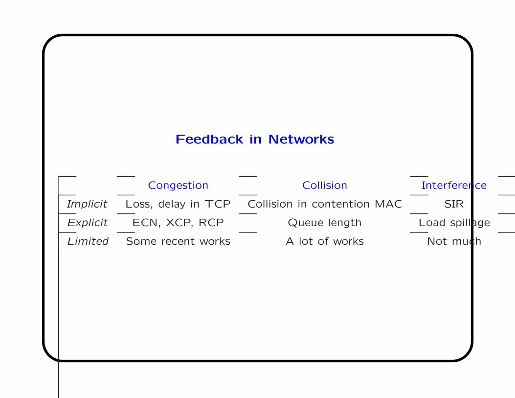
Feedback in Networks

Congestion Collision Interference

Implicit Loss, delay in TCP Collision in contention MAC SIR

Explicit ECN, XCP, RCP Queue length Load spillage

Limited Some recent works A lot of works Not much

Stochastic Noisy Feedback

0 5000 10000 150000

0.1

0.2

0.3

0.4

0.5

0.6

0.7

Iteration

Flo

w r

ate

Flow 1 (εn = 0.01)

Flow 2 (εn = 0.01)

Flow 3 (εn = 0.01)

Flow 4 (εn = 0.01)

Flow 1 (εn = 1/n)

Flow 2 (εn = 1/n)

Flow 3 (εn = 1/n)

Flow 4 (εn = 1/n)

Diminishing step size

Constant step size

Convergence properties when feedback suffers packet level corruption

(ZhangZhengChiang07)

Modeling By Reverse Engineering

Optimization of network or by network

Given a solution, what is the problem?

Forward engineering also carried out

Summary of Reverse Engineering

• TCP congestion control

One protocol: Basic NUM (LowLapsley99, RobertsMassoulie99,

MoWalrand00, YaicheMazumdarRosenberg00, KunniyurSrikant02,

LaAnatharam02, LowPaganiniDoyle02, Low03, Srikant04...)

Multiple protocols: Nonconvex equilibrium problem

(TangWangLowChiang05,06)

• IP routing:

Inter-AS routing: Stable Paths Problem (GriffinSheperdWilfong02)

• MAC backoff contention resolution: Non-cooperative Game

(LeeChiangCalderbank06)

Modeling of Topology

• Optimization-based model of network functionality on top of

random-graph models (Li Alderson Doyle Willinger 2004)

• Explanatory, rather than descriptive

A “dual” direction in Part III

Part II

Quantifying Architecture

Architecture: Functionality Allocation

Who Does What and How to Connect Them

How to contain error?

How to resolve bottleneck?

Which stock to buy: Microsoft, Cisco, Qualcomm?

Some Examples of Functionalities and Freedom

Architecture in Communication: Well-established

DecoderSource Source

EncoderChannelDecoder

Channel DestinationEncoderChannel

SourceEncoder

Rate R X’Compression X SourceDecoder

ChannelChannelDecoderEncoder

ChannelTransmission W W’

Source

Architecture in Control: Well-established

Plant

Sensor

Controller

Actuator

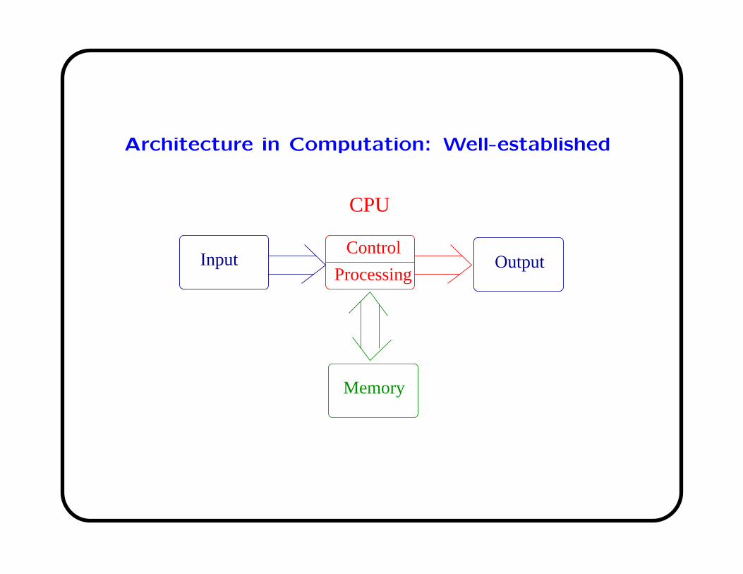
Architecture in Computation: Well-established

CPU

Input Output

Memory

Control

Processing

Architecture in Networking: Not Sure

Layer or not layer?

Application

Presentation

Session

Transport

Network

Link

Physical

Architecture in Networking: Not Sure

End-to-end or in-network?

CO

IO

SAI SAI SAI

100 Mbps

CO CO

IO

10 Gbps

1 Gbps

VHO

VHO

VHO

VHO

VHO

CO

IO

SAI

SAI

SAI

CO

CO IO

Architecture in Networking: Not Sure

Control plane or data plane?

Data

Control Signals

Math Foundation for Network Architecture

Layering As Optimization Decomposition

Network: Generalized NUM

Layering architecture: Decomposition scheme

Layers: Decomposed subproblems

Interfaces: Functions of primal or dual variables

Horizontal and vertical decompositions through

• implicit message passing (e.g., queuing delay, SIR)

• explicit message passing (local or global)

3 Steps: G.NUM ⇒ A solution architecture ⇒ Alternative architectures

Two Cornerstones for Conceptual Simplicity

Networks as optimizers

We’ve seen this in Part I

Layering as decomposition

Common language for comparing architectural alternatives

Suboptimality is fine, as long as architecture is “right”

Survey of key messages, methods, and open problems in

Proceedings of the IEEE: ChiangLowCalderbankDoyle07

Decomposition

Standard techniques of optimization decomposition:

• Dual decomposition (most widely used today)

• Primal decomposition

• Primal penalty function approach

There’re various combinations:

• Hierarchical

• Partial

• Timescale choices

User Manual for decomposition alternatives

Alternative Decompositions

XAlternative problem

representations

Different algorithms

Engineering implications

X X...

...

...

Need to explore the space of alternative decompositions

Alternative Decomposition Flowchart

Alternative FormulationsWhat functionalities and design freedoms to assume?

Alternative DecompositionsWhen and where should each functionality be done?

CoupledConstraints

More DecouplingNeeded?

Alternative AlgorithmsHow is each part of the functionalities carried out?

Cutting Plane or Ellipsoid Method

Newton (Sub)gradient

CoupledVariables

YesYes

NoNo

Yes

IntroduceAuxiliaryVariables

Primal PenaltyFunction

DualDecomposition

PrimalDecomposition

CoupledObjectives

No

Done

Yes

No

Choose DirectVariables

SpecifyObjectives

SpecifyConstraints

Physics, Technologies, and Economics

A ProblemFormulation

A CompleteSolution Algorithm

Change ofVariables

Change ofConstraints

Other Heuristics, e.g., Maximum Matching

Coupled

No

N Subproblems

Choose UpdateMethod for

eachSubproblem

Yes

DualPrimal Primal-Dual Synchronous Asynchronous

Directly Solvable orAfford Centralized Algorithm

Other AscentMethod

No

Yes

Fixed PointIteration

Choose Dynamics

Choose Time-Scales

Choose Timing

MultipleSingle

Used Dual Decomposition?

No

Yes

IntroduceAuxiliaryVariables

Need Reformulate

No

Yes

Alternative FormulationsWhat functionalities and design freedoms to assume?

Alternative DecompositionsWhen and where should each functionality be done?

CoupledConstraints

More DecouplingNeeded?

Alternative AlgorithmsHow is each part of the functionalities carried out?

Cutting Plane or Ellipsoid Method

Newton (Sub)gradient

CoupledVariables

YesYes

NoNo

Yes

IntroduceAuxiliaryVariables

Primal PenaltyFunction

DualDecomposition

PrimalDecomposition

CoupledObjectives

No

Done

Yes

No

Choose DirectVariables

SpecifyObjectives

SpecifyConstraints

Physics, Technologies, and Economics

A ProblemFormulation

A CompleteSolution Algorithm

Change ofVariables

Change ofConstraints

Other Heuristics, e.g., Maximum Matching

Coupled

No

N Subproblems

Choose UpdateMethod for

eachSubproblem

Yes

DualPrimal Primal-Dual Synchronous Asynchronous

Directly Solvable orAfford Centralized Algorithm

Other AscentMethod

No

Yes

Fixed PointIteration

Choose Dynamics

Choose Time-Scales

Choose Timing

MultipleSingle

Used Dual Decomposition?

No

Yes

IntroduceAuxiliaryVariables

Need Reformulate

No

Yes

The impact of imperfect scheduling on cross-layer r ate control In wireless networks, Xiaojun Lin and Ness B. Shroff , ToN’06

CAD Tool

Automate the enumeration of alternative decompositions:

Automate the comparison of alternative decompositions:

• Speed of convergence

• Robustness (errors, failures, network dynamics)

• Message passing (amount, locality, symmetry)

• Local computation (amount, symmetry)

• Ease of relaxing to simpler heuristics

• Ease of modification as new applications arise

Challenge: Some of the following metrics are not well defined, fully

quantified, or accurately characterized

The Challenge of Coupling

Not every coupling is dual-decomposable

There are much tougher coupling:

• Objective function: network lifetime or coupled utilities

• Constraint: Perron-Frobenius eigenvector in power control

Case 1: DSL Spectrum Management

DMT (Discrete Multi−Tone) Transmissions

Fiber

Copper Line

Downstream Transmission

IP and PSTN Network

crosstalk

TX

TX RX

RX

Customer 2

CO

RT

Customer 1

Dynamic Spectrum Management

Problem formulation to characterize rate region

maximizeP

n wnRn

subject to Rn =P

k log

„

1 +pk

nP

m 6=n αkn,mpk

m+σkn

«

P

k pkn ≤ Pmax

n ,∀n

• Nonconvex

• Coupled across users

• Coupled across tones

History

• IW: Iterative Water-filling [Yu Ginis Cioffi 02]

• OSB: Optimal Spectrum Balancing [Cendrillon et. al. 04]

• ISB: Iterative Spectrum Balancing [Liu Yu 05] [Cendrillon Moonen 05]

• ASB: Autonomous Spectrum Balancing [Cendrillon Huang Chiang

Moonen TransSignalProc06]

• Many other work: BPM, SCALE, IW variants...

Algorithm Operation Complexity Performance

IW Autonomous O (KN) Suboptimal

OSB Centralized O`

KeN´

Optimal

ISB Centralized O`

KN2´

Near Optimal

ASB Autonomous O (KN) Near Optimal

K: number of carriers N : number of users

Solution Idea: Static Pricing

Dynamic pricing for dynamic coupling: decouple tones

Static pricing for static coupling: decouple users

Actual Line

Reference Line

CO

CPCO

RT CP

RT

RT

CP

CP

CP

Same convergence conditions as iterative-waterfilling proved

Much Larger Rate Region (Marvell Simulator)

0 1 2 3 4 5 6 7 80.4

0.6

0.8

1

1.2

1.4

1.6

1.8

2

User 4 achievable rate (Mbps)

Use

r 1

achi

evab

le r

ate

(Mbp

s)

Optimal Spectrum BalancingIterative Spectrum BalancingAutonomous Spectrum BalancingIterative Waterfilling

Case 2: Wireless Network Power Control

0 1 2 3 4 5 6 7 8 9 100

2

4

6

8

10

12

QoS 1

QoS

2

Utility Level Curves

Maximize: utility function of powers and SIR assignments

Subject to: SIR assignments feasible

Variables: transmit powers and SIR assignments

History

• Late 1980s: Qualcomm’s received power equalization for near-far

problem

• 1992-2000 Fixed SIR: distributed power control:

Zander 1992, Foschini Miljanic 1993, Mitra 1993, Yates 1995, Bambos

Pottie 2000 ...

• Late 1990s: 3G for data wireless networks

• 2001-2004 Nash equilibrium for joint SIR assignment and power

control:

Saraydar, Mandayam, Goodman 2001, 2002, Sung Wong 2002, Altman

2004 ...

• 2004-2005 Centralized computation for globally optimal joint SIR

assignment and power control:

O’Neill, Julian, and Boyd 2004, Chiang 2004, Boche and Stanczak 2005

• 2006 Distributed and optimal joint control:

Hande Rangan Chiang Infocom06

Load-Spillage Power Control (LSPC)

Reparameterization: From right eigenvector to left eigenvector:

Initialize: Arbitrary s[0] ≻ 0.

1. BS k broadcasts the BS-load factor ℓk[t] =P

i∈Sksi[t].

2. Compute the spillage-factor ri[t] byP

j 6=i,j∈Sσisj +

P

k 6=σihkiℓk.

3. Assign SIR values γi[t] = si[t]/ri[t].

4. Measure the resulting interference qi[t].

5. Update (in a distributed way) the load factor si[t]:

si[t + 1] = si[t] + δ∆si[t].

where ∆si =U ′

i(γi)γi

qi− si

Continue: t := t + 1.

Convergence and Optimality

Theorem: For convex SIR feasibility region, and sufficiently small step

size δ > 0, Algorithm converges to the globally optimal solution of

maximize U(γ)

subject to ρ(D(γ)G) ≤ 1

Proof: Key ideas:

• Develop a locally-computable ascent direction (most involved step)

• Evaluate KKT conditions

• Guarantee Lipschitz condition

Extend to joint beamforming and bandwidth allocation

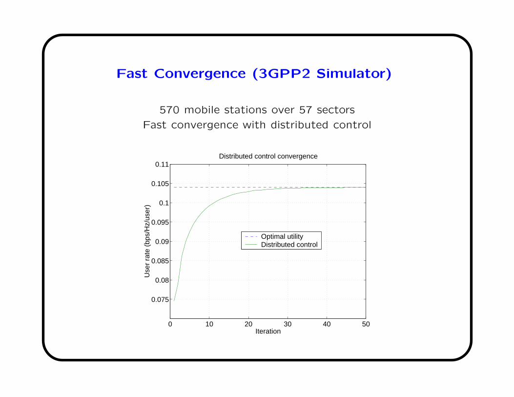
Fast Convergence (3GPP2 Simulator)

570 mobile stations over 57 sectors

Fast convergence with distributed control

0 10 20 30 40 50

0.075

0.08

0.085

0.09

0.095

0.1

0.105

0.11

Iteration

Use

r ra

te (

bps/

Hz/

user

)

Distributed control convergence

Optimal utilityDistributed control

Part III

Robustness to Stochastic Dynamics

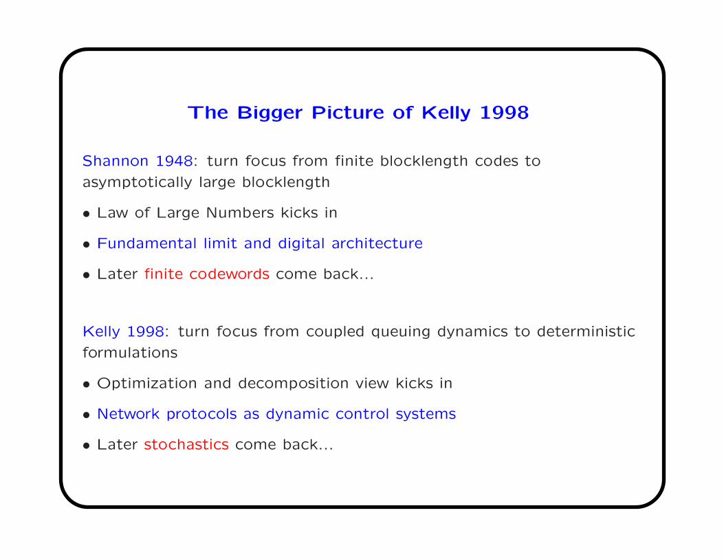
The Bigger Picture of Kelly 1998

Shannon 1948: turn focus from finite blocklength codes to

asymptotically large blocklength

• Law of Large Numbers kicks in

• Fundamental limit and digital architecture

• Later finite codewords come back...

Kelly 1998: turn focus from coupled queuing dynamics to deterministic

formulations

• Optimization and decomposition view kicks in

• Network protocols as dynamic control systems

• Later stochastics come back...

Stochastic Network Utility Maximization

Filling in the table with 3 stars would be a long-overdue union between

stochastic networks and distributed optimization (survey in YiChiang07)

Stability or Average Outage Fairness

Validation Performance Performance

Session Level ⋆⋆ ⋆ ⋆

Packet Level ⋆ ⋆

Channel Level ⋆⋆ ⋆

Topology Level

Timescale of interactions is crucial

Only look at box (1,1) in this talk

Session Level Stochastic Stability

Dynamic user population with arrivals and departures

maximizeP

s Ns(t)U(φs/Ns(t))

subject to φ ∈ R

• If Poisson (λ) arrival with exp (1/µ) filesize distribution:

Number of active sources follows Markov chain:

Ns(t) → Ns(t) + 1 with rate λs

Ns(t) → Ns(t) − 1 with rate µsφs(N(t),R)

Queue/rate stability of M/SD/1/∞ queuing network

λ/µ ∈ R is necessary, is it also sufficient?

Stability I: Simple Constraint Set

Work Arrival Topology Ui U shape

de Veciana et.al. 99 Poisson, Exp General Same α = 1,∞

Bonald Massoulie 01 Poisson, Exp General Diff. General

Lin Shroff, Srikant 04 Poisson, Exp General Same α > 1

Fast timescale

Ye et.al. 05 Exp filesize General Diff. General

Bramson 05 General General Same α = ∞

Lakshmikantha et.al. 05 Phase type 2 × 2 grid Same α = 1

Massoulie 06 Phase type General Same α = 1

Gromoll Williams 06 General Tree Same General

Chiang Shah Tang 06 General General Diff. A range of α

Open General General Diff. All α

Stability II: General Constraint Set

φ1

φ2

φ1 φ1

φ2φ2

(a) convex rate region (b) nonconvex rate region

rate region

maximum stability region

stability region for small α

stability region for large α

(c) time-varying

rate regions

Convex rate region case: stability region is rate region

What about nonconvex or time-varying rate region?

(LiuProutiereYiChiangPoor-Sigmetrics07)

May not be maximum stability region and sensitive to α

Stability-Fairness Tradeoff

0 0.5 1 1.5 2 2.5 30

0.5

1

1.5

2

2.5

3

class 1

clas

s 2 α=0.1

α=0.3α=0.7α=1α=1.5

0 0.5 1 1.5 2 2.5 30

0.5

1

1.5

2

2.5

3

class 1cl

ass

2

α=0.2α=0.5α=0.7α=1α=2

α=5α=10α=100

More fair allocation has smaller stability region

when rate region is time-varying

Proof Techniques

• Fluid limit proof

• Laypunov function construction

• Max projection and monotone cone policy

Open Problems

• Fluid model or fluid limit?

• Does P2P and IPTV traffic require different models?

• How many flows is “many-flow”?

• Design for topology level stochastics?

• From convergence to equilibrium to invariance during transience

Part IV

DFO

Design For Optimizability

Nonconvexity happens:

• Nonconcave utility (eg, real-time applications)

• Nonconvex constraints (eg, power control in low SIR)

• Integer constraints (eg, single-path routing)

• Exponentially long description length (eg, certain scheduling)

Mathematically, convexity not invariant, so we can have, e.g.,

• Sum-of-squares method (Stengle73, Parrilo03)

• Geometric programming (DuffinPetersonZener67)

More engineering approach: Design for Optimizability

Tackling Nonconvexity

Option 1: Go around nonconvexity

• Geometric Programming, change of variable

• Sufficient condition under which the problem is convex

• Sufficient conditions for uniqueness of KKT points

Tackling Nonconvexity

Option 2: Go through nonconvexity

• SOS, Signomial programming, successive convex approximation

• Special structure (e.g., DC, generalized quasiconcavity)

• Canonical duality, Smart branch and bound, etc.

Tackling Nonconvexity

Option 3: Go above nonconvexity: Design for Optimizability

Change difficult optimization problem, rather than solve it

• Redraw architecture or protocol to make the problem easy to solve

• Need to balance with the cost of making changes to protocols

Optimization as a flag to design issues

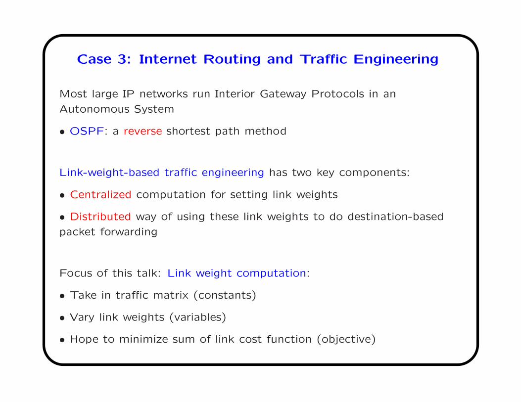
Case 3: Internet Routing and Traffic Engineering

Most large IP networks run Interior Gateway Protocols in an

Autonomous System

• OSPF: a reverse shortest path method

Link-weight-based traffic engineering has two key components:

• Centralized computation for setting link weights

• Distributed way of using these link weights to do destination-based

packet forwarding

Focus of this talk: Link weight computation:

• Take in traffic matrix (constants)

• Vary link weights (variables)

• Hope to minimize sum of link cost function (objective)

Internet Routing and Traffic Engineering

Network (Link-state routing)

Operator (Compute link weights)

Traffic matrix

measure Link capacity

link weights Desirable traffic

distribution

3

2

2

1

1

3

1

4

5

3

Path length= 8

History

• 1980s-1990s, intra-domain routing algorithms based on link weights

• 1990s, many variants of OSPF proposed and used: UnitOSPF,

RandomOSPF, InvCapOSPF, L2OSPF

• Late 1990s, more complex MPLS protocols proposed. (Optimal

benchmark: arbitrary splitting of flows on any links in any proportion),

but they lose desirable features, eg, distributed determination of flow

splitting and ease of management

• 2000, Fortz and Thorup presented local search methods to

approximately solve the NP-hard problem in OSPF

• 2003, Sridharan, Guerin, and Diot proposed to select the subset of

next hops for each prefix

• 2005, Fong, Gilbert, Kannan, and Strauss proposed to allow flows on

non-shortest paths, but loops may be present and performance under

multi-destination scenarios not clear

• 2007, Xu, Chiang, Rexford propose DEFT and show achievability of

optimal traffic engineering

From OSPF to DEFT

A new way to use link weights (XuChiangRexford-Infocom07):

• Use link weights to compute path weights

• Split traffic on all paths

• Exponential penalty on longer paths

Same way to do (destination-based) packet forwarding

How good can the new protocol be?

How to compute link weights in the new protocol?

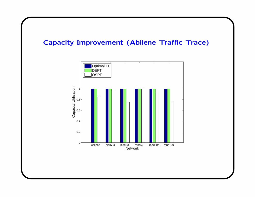
Capacity Improvement (Abilene Traffic Trace)

abilene hier50a hier50b rand50 rand50a rand1000

0.2

0.4

0.6

0.8

1

Network

Cap

acity

Util

izat

ion

Optimal TEDEFTOSPF

Optimality Gap Reduction

abilene hier50b rand100

0.05 0.1 0.15 0.20

100

200

300

400

500

600

700

800

900

Network Loading

Opt

imal

ity G

ap (

%)

OSPFDEFT

0.02 0.03 0.04 0.05 0.060

50

100

150

200

250

Network Loading

Opt

imal

ity G

ap (

%)

OSPFDEFT

0.08 0.1 0.12 0.14 0.16 0.180

20

40

60

80

100

120

140

160

180

200

Network Loading

Opt

imal

ity G

ap (

%)

OSPFDEFT

Simple Routing Can Be Optimal

Theorem: Link state routing and destination-based forwarding can

achieve optimal traffic engineering

Theorem: Optimal weights can be computed in polynomial time

Gradient algorithm solves the new link weight optimization problem

2000 times faster than local search algorithm for OSPF link weight

computation

Solution Idea: Network Entropy Maximization

Feasible flow routing

Optimal flow routing

Realizable with link-state routing

Constraint: flow conservation with effective capacity

Objective function: find one that picks out only link-state-realizable

traffic distribution

Entropy function is the right choice, and the only one

Nonconvexity Can Be Sweet

Sometimes, hard problems aren’t hard in reality. When?

Sometimes, hard problems don’t deserve to exist. How?

Solve Hard Problems

restrictive non-scalable

solution assumption formulation intractable

Don’t Solve Hard Problems

restrictive non-scalable

solution assumption formulation intractable

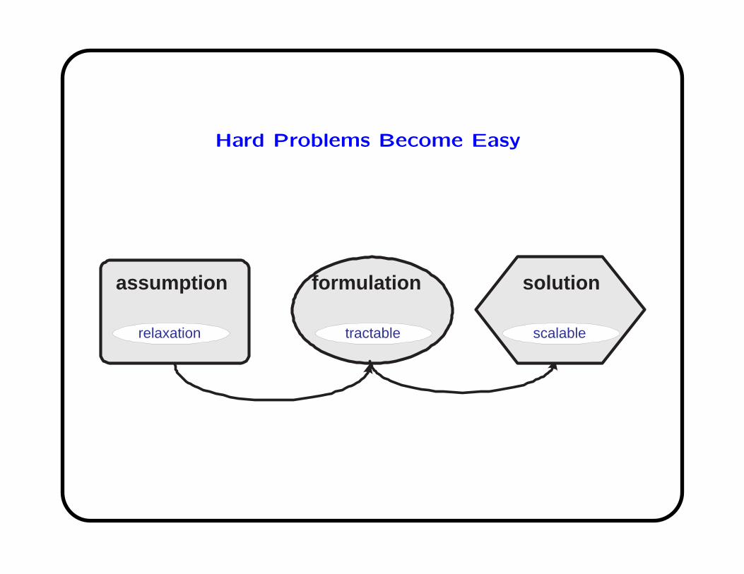
Hard Problems Become Easy

relaxation scalable

solution assumption formulation

tractable

Feedback in Engineering Process

restrictive

relaxation

non-scalable

scalable

solution assumption formulation intractable

tractable

Optimizability-Complexity Tradeoff

Often there is a price for revisiting assumptions

In Internet traffic engineering case, DFO provides the best possible

tradeoff

simple

o p t i m

a l

MPLS

OSPF

DEFT

Part V

Complexity

Beyond Optimality

I. Modeling: Resource allocation, fairness, reverse-engineering

II. Architecture: who does what and how to connect

III. Robustness to stochastic dynamics

IV. Feedback to engineering assumptions

V. Complexity-performance tradeoff

Optimization as a language to think about network engineering

Contacts

[email protected]

www.princeton.edu/∼chiangm