Beyond Bathymetry: Probing the Ocean Subsurface Using Ship-Based LIDARs

Beyond Bathymetry: Probing the Ocean Subsurface Using Ship-Based LIDARs

Charles C. Trees

NATO Centre for Maritime Research and Experimentation (CMRE)

La Spezia, Italy

ABSTRACT

This document outlines a ‘proof-of-concept’ for the maritime application of a ship-based LIDAR system for measuring

the optical and physical properties in the water column. It is divided up into sections, documenting that there exists

today the engineering, modeling and optical expertise to accomplish this task as well as a discussion of the reasons that

LIDAR has not become the powerful observational platform that it should have been for horizontally and vertically

monitoring optical and physical water column properties. Previous research on this approach has been limited because

LIDAR systems have for most cases not been thoroughly calibrated, if at all, nor have LIDARs been focused on

above-water, ship-based measurements. Efforts at developing derived product algorithms with uncertainties have been

limited. This review concludes that there is a huge potential for the successful application of LIDAR measurements in

the marine environment to estimate the vertical distribution of optical and physical properties and that measurement

costs can be minimized by deployment of these automated systems on ‘ships-of-opportunity’ and military vessels on a

non-interfering basis. Although LIDAR measurements and research have been around since the 1960’s, this approach

has not really been investigated by any civilian or military agencies or laboratories even though providing ‘through-

sensor performance matrixes’ for existing bathymetry, target detection, underwater communication and imaging

should be high on their list.

Keywords: LIDAR, calibration and characterization, ship-based, in-situ, optical modeling, ground truth.

1. INTRODUCTION

LIght Detection And Ranging (LIDAR) systems have been used successfully in the past to reveal the biological

vertical structure (e.g. plankton and fish distributions) as well as providing geographic and physical mapping products,

such as bathymetry, internal waves and suspended particles. In the past the focus areas for LIDARs has been the

generation of civilian Digital Elevation Maps (DEM) of land, ice and coastal shoreline as well as additional military

applications for bathymetry, mine detection and Anti-Submarine Warfare (ASW). What has received little research

effort is the application of LIDAR measurements to estimate the optical (Inherent Optical Properties, IOPs and

Apparent Optical Properties, AOPs) and physical (e.g. turbulence, temperature, salinity, sound speed) properties

within the upper surface of the water column. A quick explanation for this deficiency is that the maritime customers

were not interested in mapping the environmental characteristics of the water column other than estimating bottom

depth (sometimes bottom reflectance) and target detection and discrimination. For both bathymetric and target

detection systems, LIDAR return signals are large and therefore for this application it requires very little ground

truthing or calibration of the systems as the signal to noise (S/N) is always high giving the greatest penetration depth

e.g. a hard target can be seen at deeper depths than a soft one with the same system). As measurement consistency

between various LIDAR systems and ‘through-sensor’ knowledge of depth penetration and associated uncertainties are

requested by users, calibration and derived product validation will become important components of mapping and

intelligence reconnaissance efforts. Additionally, as targets become more difficult to detect based on placement

(burial, surface zone, coastal fronts), exterior covering and structure (bio-fouling, sediment deposition, camouflage,

roughness), LIDAR systems will be required to detect small changes between targets (subtle differences in intensity

and wavelength require characterization and calibration, C2) and provide robust and accurate algorithms to convert

retrieved waveforms into products (e.g. diver visibility, bathymetry, target location and identification, internal waves,

mixed layer depth, thin turbid layers) no matter which LIDAR system is deployed there must be interoperability and

standardization between systems. LIDARs can also be used on AUVs to assist in improving underwater imaging (e.g.

laser scanning cameras) by estimating optical properties in the water column, thus predicting the maximum distance Ocean Sensing and Monitoring VI, edited by Weilin W. Hou, Robert A. Arnone, Proc. of SPIE Vol. 9111, 91110U · © 2014 SPIE · CCC code: 0277-786X/14/$18 · doi: 10.1117/12.2053875

Proc. of SPIE Vol. 9111 91110U-1

Downloaded From: http://proceedings.spiedigitallibrary.org/ on 05/19/2015 Terms of Use: http://spiedl.org/terms

from the target to minimize false targets and to effectively discriminate between target and surrounding clutter with the

possibility of target identification through visualization.

Sensor characterization and calibration (metrology) efforts, although time consuming with reoccurring costs (as they

need to be performed regularly depending upon deployment frequency), can be easily implemented once C2 optical

protocols have been developed by National Laboratories (e.g. National Institute of Standards and Technology

(NIST/NOAA), USA, and National Physical Laboratory (NPL), GBR). The development of robust algorithms to

relate LIDAR return signals to optical and physical properties and determine their uncertainties requires a different

approach than previously used for LIDAR ground truth data collection. Past LIDAR research generally utilized

aircraft 1,2,

3) and space-based platforms

4,5, which are limited in the number of paired observations, since these

platforms have such short temporal measurement periods (one paired ground truth data point per overpass, although

they are advantageous because of the extended spatial coverage). Ship-based deployment is required to provide robust

derived products from retrieved LIDAR signals, where other observational platforms can be deployed simultaneously

with the LIDAR scans. During a ship transit, towed vehicles are invaluable platforms for collecting horizontal and

more importantly vertical optical and physical data. While on station, LIDAR comparisons can be made with profiling

optical and physical instrumentation to provide robust derived product algorithms as well as uncertainty budgets for

these products. Ship-based validations with a C2 LIDAR system are the first steps in developing it into a powerful

observational tool.

2.APPLICATION TO MARITIME ENVIRONMENT

2.1 Depth penetration There is generally a ‘rule of thumb’ that LIDAR return signals can penetrate down to three optical depths (OD=).

This is a conservative estimate of penetration depth that is based on optical properties of the water column and more

importantly on the strength of the backscattered signal. Penetration depth is also dependent on the laser wavelength

and marine environment to be monitored [green laser at 532nm for littoral and coastal areas, blue laser at 450-490nm

for open ocean waters and yellow laser at >560nm for turbid waters). For hard targets, such as the sea floor, the

estimate is closer to four optical depths (ODs), whereas estimating optical properties from the decay in the LIDAR

signal it is closer to three ODs. The diffuse optical depth, (z), is defined as

(z) = ln (Eo/Ez) = Kz, 1

where ‘o’ and ‘z’ subscripts are the downwelling irradiance incident at the surface and at some depth (z), respectively,

and K is the diffuse attenuation coefficient (m-1

). When the OD, (z) is equal to 1.0 then the depth at which this

occurs is equal to inverse of the diffuse attenuation coefficient (1/K) which is also the 37% light level depth and the

depth at which 90% of the remotely sensed ocean color signal originates. K(490) is a standard derived product that

has been generated from most satellite-based ocean colors sensors, such a SeaWiFS, MODIS, MERIS, VIIRS, etc. It

can be demonstrated that a conventional airborne LIDAR systems can retrieve data as deep as the mixed layer depth

(MLD) by using satellite derived global maps of K distributions in conjunction with the US Navy’s NCOM model that

predicts MLD6. Assuming that the optical properties retrieved in the upper water column (37% light level depth or

1/K) by SeaWiFS are indicative of the water clarity down to the MLD, then LIDARs can be used to measure through

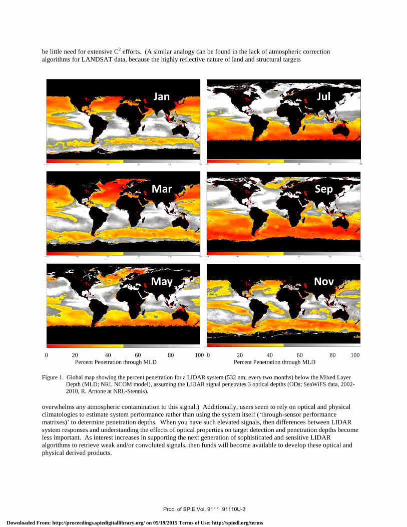
the thermocline/MLD for ~70% of the world’s oceans annually (Fig. 1). So LIDAR surveying has the potential to

retrieve optical and physical properties down to and through the MLD for a significant portion of oceanic coastal

areas. This capability to provide a Rapid Environmental Assessment (REA) has many important military and civilian

applications, with the obvious being improved ocean modelling and forecasting through data assimilation optical and

physical properties. It should be emphasized that retrieving optical and physical properties above the MLD is also

important for these and other applications (bioluminescence, gas exchange, near surface algal blooms, diver visibility,

etc.).

2.2 Characterization and calibration (C2) Now that it has been shown that LIDAR surveys are capable of sampling down to and even through the MLD in most

areas, the issue about characterization and calibration (C2) will be addressed. The same reasons stated above about the

lack of funding for extraction of optical properties from the LIDAR signals can also be used to explain the limited, if

any, C2 efforts. With the large LIDAR return signals from hard targets such as the sea floor and mines, there seems to



100

be little need for extensive C2 efforts. (A similar analogy can be found in the lack of atmospheric correction

algorithms for LANDSAT data, because the highly reflective nature of land and structural targets

0 20 40 60 80 100 0 20 40 60 80 100

Percent Penetration through MLD Percent Penetration through MLD

Figure 1. Global map showing the percent penetration for a LIDAR system (532 nm; every two months) below the Mixed Layer

Depth (MLD; NRL NCOM model), assuming the LIDAR signal penetrates 3 optical depths (ODs; SeaWiFS data, 2002-

2010, R. Arnone at NRL-Stennis).

overwhelms any atmospheric contamination to this signal.) Additionally, users seem to rely on optical and physical

climatologies to estimate system performance rather than using the system itself (‘through-sensor performance

matrixes)’ to determine penetration depths. When you have such elevated signals, then differences between LIDAR

system responses and understanding the effects of optical properties on target detection and penetration depths become

less important. As interest increases in supporting the next generation of sophisticated and sensitive LIDAR

algorithms to retrieve weak and/or convoluted signals, then funds will become available to develop these optical and

physical derived products.

Jan

Mar

May

Jul

Sep

Nov



There have been only a few published articles on efforts to radiometrically calibrate LIDAR systems and none on

laboratory characterization of the system components. Without a thorough characterization of the LIDAR system it

becomes difficult to develop a model to simulate the LIDAR waveform as the system specifications are not accurately

known or verified. One of the first documented calibration efforts was performed on the US Navy’s SHOALS

(Scanning Hydrographic Operational Airborne Lidar Survey)7. They suggested that water column optical properties

could be estimated from SHOALS data by fitting recorded waveforms to modelled simulated waveforms. The values

of the optical parameters providing the best fit were accepted as estimates of these desired parameters. Consequently,

the success of this ‘fitting’ technique requires the calculation of the simulated optical signal into an electrical signal

recorded by the LIDAR digitizer and therefore the system must be calibrated. Tuell et al. (2005)7 used an 80m

calibration facility and recorded the signals received as the laser pulses varied in power. This required the addition of

a calibrated power meter to simultaneously monitor the laser intensity reflected from a wall that had painted tiles

attached to it. By putting a variety of neutral density filters in front of the LIDAR optical receiver, they were able to

reduce the return power measured by SHOALS.

The other published calibration effort was by Lee et al. (2013)8 working with NOAA’s Fish Lidar

9. They also

proposed that a simulated model of the dependence of the LIDAR signal on the optical properties of the water was

necessary to invert the LIDAR return. The first calibration effort was in the laboratory where the transmission of the

optics for all receiver channels, the response of each PMT as a function of applied gain-control voltage and the

response of the logarithmic amplifier was measured separately. Measuring the individual component parts of an

optical instrument and then assuming that summing these components together will provide a calibration quality

instrument is not a correct assumption. This approach can only be used to qualitatively estimate the characterization of

the LIDAR system. For a thorough C2 all optical components should be assembled and then simultaneously tested in

the calibration laboratory with radiometric standards.

For the next phase of the calibration, a horizontal propagation range at 300 m was used and instead of neutral density

filters to reduce the laser power several different targets with known and calibrated reflective surfaces (Spectralon)

were used. They also recorded the impulse response function of the system, which included the effects of the laser

pulse shape and the low-level ringing of the logarithmic amplifier. Unfortunately, there was no mention of the

addition of a calibrated power meter to measure the laser intensity at the Spectralon plaque and this is a limitation.

Since Spectralon plaques are expensive to purchase as compared to neutral density filters7, one would have to assume

that the range of laser powers used for the development of a calibration curve by Lee et al. (2013)8 was not as

extensive as the SHOALS effort. Because of these calibrations, both LIDAR groups were able to successfully

simulate the LIDAR return signals and thus extract qualitative estimates of diffuse attenuation [K(532)] and absorption

coefficients [a(532)]. So LIDAR calibrations can be performed, but there is a requirement that optical calibration

protocols be developed and agreed upon by the metrologists. The characterization of LIDAR systems has received

little to no attention, so this ‘proof-of-concept’ document recommends that C2 protocols be established and that the

calibration efforts be performed on a regular basis, depending upon the usage and number of deployments of each

LIDAR.

2.3 Modelling LIDAR waveforms As mentioned above in the LIDAR C

2 examples, there is a requirement to model and simulate LIDAR waveforms in

order to obtain accurate estimates of water column optical properties as well as seafloor reflectance parameters. The

conversion of the LIDAR waveforms into optical properties requires an inversion of the oceanic LIDAR return

(inverse model) because the LIDAR signal is a function of the attenuation [c()] and backscattering [bb()]

characteristics of the water column. This becomes convoluted in that the laser pulse is reduced as a function of c()

and bb() on its downward path, but for the return path the signal decay is now a function of the diffuse attenuation

[K()] and bb(). Although both c() and K() are functions of the absorption and scattering properties in the water

column, they are distinctly different attenuation properties. c() is an Inherent Optical Property (IOP) and is related to

the absorption [a()] and the scattering [b()] coefficients in the form of

c() = a() + b(). 2

K() on the other hand is an Apparent Optical Property (AOP) and is governed by the incident solar and sky

illumination such that the relationship to a() and b() is of the form

K() = a() + b()/n, 3



where’ n’ is a fraction of scattered light [for those photons scattered “out” of the instruments Field-of View (FOV)

there are photons from adjacent regions which are scattered back “in”]. K() is always less than the magnitude of c()

with the difference depending upon the relative proportions of a() and b() in the water column. Also be aware that

the above attenuation equations do not contain the backscattering coefficient [bb()], although b(), the total scattering

coefficient, is a function of the forward scattering plus the backscattering coefficients [b() = bf() + bb()]. Besides

this difference in attenuation properties between the downward and the upward backscattered laser pulse decays, the

FOV of the optical receiver on the LIDAR also determines the sensitivity of the system to K() or c(). For narrow

FOVs (1-4o) the LIDAR signal is governed more by c(), whereas for larger FOVs (e.g. 8-12

o) K() determines the

attenuation of the laser signal. These are the reasons for optical modeling of LIDAR waveforms to extract optical

properties.

There have been several published LIDAR models that can be used to simulate the LIDAR return waveform using

optical properties as input to this solution. A few of these models will now be discussed, like Dolina et al. (2007)9 that

utilized previously published optical relationships to develop algorithms for solving the LIDAR inverse problem using

correlations between IOPs10

. They found errors ranging from 10% to 40% in retrieving c() with the smaller errors

occurring in the near surface layers (1-2 ODs) and the larger ones at greater ODs (3-5). Improved accuracies of the

retrieval of IOPs can be made if a more precise relationship can be found between b() and c() in the regions of

observations. They proposed an adaptive algorithm approach to improve the retrieval accuracy by processing the

LIDAR signal itself and a priori knowledge of the IOP distribution and variability.

Another LIDAR model used with NAVAIR’s K-Meter Survey System (KSS) was the KSS-2 model11

. The KSS

LIDAR was designed to obtain system specific attenuation coefficients (Ksys), as well as investigating the potential for

determining other water column IOPs. Inputs into the KSS-2 model were the system configurations (FOV, etc.),

system geometries (altitude, etc.), transmit/receive characteristics, atmospheric visibility, sea surface conditions, water

column optical properties (stratification) and phase function. The outputs were LIDAR return profiles including the

components of the return profile (atmosphere, surface, water), LIDAR decay rate [Ksys(z)] and shot and surface noises.

The agreement between modelled and measured waveforms were excellent in both clear (c = 0.27 m-1

) and turbid (c =

1.6 m-1

) waters with the model results being within the model input errors. Several years later Zege et al. (2003)12

developed new software [Airborne Oceanic Lidar Simulator (AOLS)] to support quasi-real-time simulation of airborne

LIDAR performance based on an underlying semi-analytical theory of a LIDAR return with multiple scattering. This

model provides the simulated signals for elastic-backscatter LIDAR with polarization devices and with Raman and

fluorescence channels.

The last modeling approach discussed13,14

uses the small-angle scattering approximation in the Radiation Transfer

Equation (RTE) to form the basis of an accepted model of LIDAR performance. This “multiple-forward-single-

backscattering” model is used to develop techniques for estimating backscattering coefficients, beam attenuation

coefficients, single-scattering albedos and the Volume Scattering Function (VSF) asymmetry coefficients by fitting

simulated waveforms to actual data measured by two LIDAR receivers (a shallow water APD receiver with an 18mrad

FOV and a deep water Photomultiplier Tube (PMT) receiver with a 40mrad FOV). Remember that small and large

FOV sensors have different attenuation coefficients (K vs c) that affect the decay rates of the LIDAR waveforms.

So several inverse models have been presented that can be used to evaluate LIDAR system performance as well as

estimating optical properties in the water column. Most of the LIDAR modeling and optical expertise has been

developed in Russia and Belarus as they have been the leaders in LIDAR research for many decades. Many of these

key LIDAR modeling experts (Drs, Eleonora Zege11,12

, Lev S. Dolin9, Oleg Kopelevich

10 and Yuri Kopilevich

7,13,14)

attended the Centre sponsored LIDAR Observations of Optical and Physical Properties (LOOPP) Workshop in 2011 in

La Spezia, Italy.

2.4 Optical properties estimated from LIDAR waveforms As previously stated in Section 3.2, most approaches at estimating in-situ optical properties from LIDAR signals

require a model that simulates the actual measured waveform by inputting a variety of optical parameters into the

model. If the simulated waveforms accurately represent the measured LIDAR signal then the optical properties can be

retrieved from the model. Correlation approaches that relate the actual LIDAR signal to optical properties don’t seem



to be a very effective method for retrieving the vertical distribution of these properties9. So what we will present in

this section are results from modeling LIDAR waveforms and then extracting optical properties from that simulated

waveform model. Most of the comparisons presented will be of a qualitative nature because of the lack of C2 and the

limited number of concurrently acquired optical and LIDAR measurements. As previously stated, ship-based systems

have the best chance of improving the predictive potential for LIDARs to vertically profile optical data.

Using an airborne polarized LIDAR system, Vasilkov et al. (2001)15

investigated the ability of a LIDAR system that

measured the two orthogonal-polarized components of the backscatter light pulse to retrieve vertical profiles of the

backscattering coefficient [bb(532)]. Rationale for this polarized technique is that depolarization of backscattered light

originating from a linearly polarized laser beam, is dominated by multi-angle scattering from particles in the water

column. The magnitude of this small-angle scattering is determined by bb(532). This was a joint Russian-American

LIDAR Experiment which showed that the retrieved profiles of bb(532) only reproduced the main features of the

measured profiles of the beam attenuation coefficient, c(532). Accuracies for this optical retrieval were not given.

The system specific or effective attenuation coefficient K(532) from three LIDAR pulses were 0.139, 0.120 and

0.088m-1

and had correlation coefficients of 0.994, 0.993 and 0.984, respectively.

Tuell et al. (2005)7 investigated the ability of the SHOALS LIDAR system to estimate water-column optical properties

and seafloor reflectance (532 nm) during aircraft overflights off Fort Lauderdale, Florida, USA in November 2003. As

discussed in the modeling section above, SHOALS utilizes a two receiver system [Avalanche Photodiode Detector

(APD) and Photomultiplier Detector (PMT)] to assist in estimating bb(532). They provided no estimate of the vertical

distribution of the absorption and scattering coefficients from the modeled LIDAR waveforms, but did compare

LIDAR integrated optical properties with vertical measurements from a Wet Labs Absorption and Attenuation Meter

(ac-9). The SHOALS system estimated a(532) and b(532) to be 0.089m-1

and 0.227m-1

, respectively, as compared to

the mean near-surface values from ac-9 measurements of 0.070m-1

and 0.218m-1

, respectively.

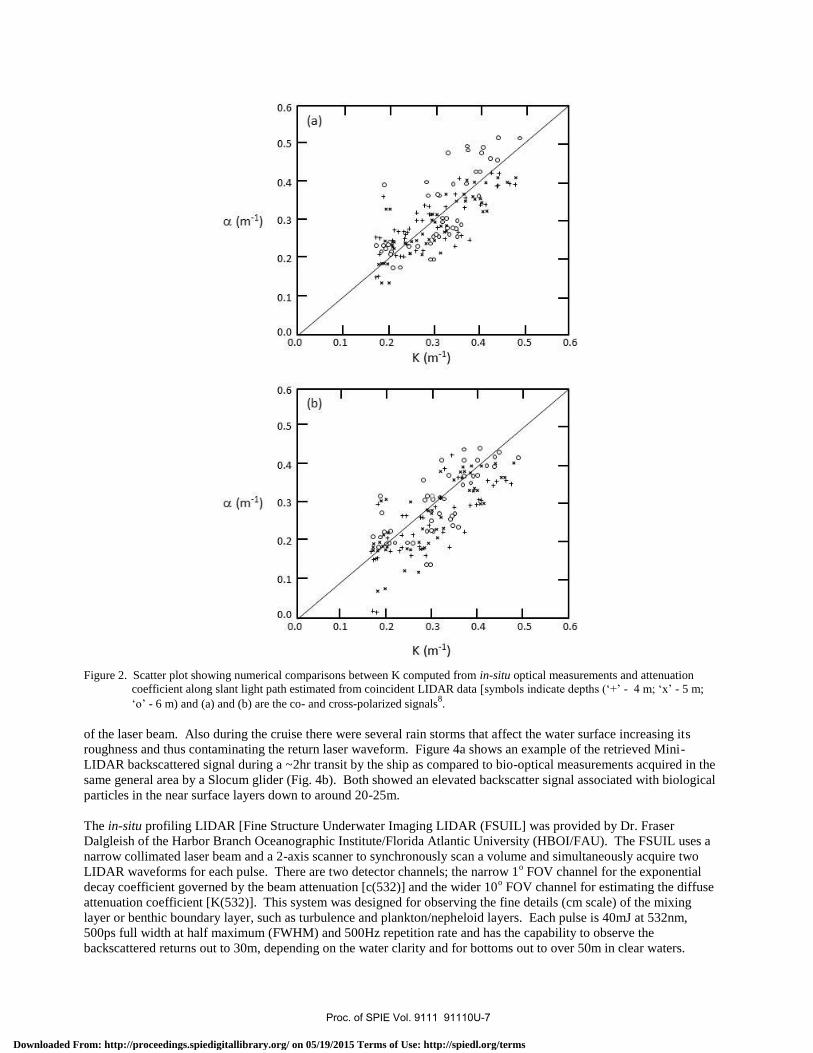
The most in depth article on the comparison of LIDAR measurements with in-situ optical profile data is the work by

Lee et al. (2013)8. The airborne LIDAR deployed was NOAA’s Fish Lidar, which measures the LIDAR waveforms

for both the co-polarized and cross-polarized return. Sixty in-situ optical profiles were correlated with nearly

collocated and coincident LIDAR profiles, with their quasi-single-scattering simulated model providing good

agreement to the measured LIDAR waveforms. Figures 2a, b show the comparisons between the diffuse attenuation

coefficients, K(532), computed from in-situ absorption and attenuation measurements (ac-9) and the attenuation

coefficients [ (532)] estimated from the LIDAR decay rates for both co-polarized (2a) and the cross-polarized signals

(2b). These relationships seem to be quite good over optical values with the average /K ratio being 1.05 + 0.02 and

0.92 + 0.02 for the co- and cross-polarized returns, respectively. The variance in these relationships is large and much

of this may be due to the fact that the authors used IOP data (ac-9) to estimate and the diffuse attenuation coefficient,

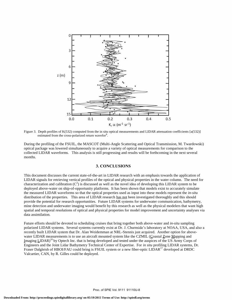
K(532). A plot of the estimated K(532) as a function of depth is shown in Fig. 3 for the upper 15 meters. K(532) has

an average value of 0.2m-1

throughout the water column with the range in estimated K(532) being + 0.5m-1

. K profiles

are generally smooth because they represent the integrated value of the loss of diffuse light with depth, so much of the

variability seen in Fig. 3 can be attributed to the estimate of K from IOPs as well as extracting attenuation from the

decay of the LIDAR return at small depth intervals.

2.5 Ligurian Sea LIDAR and Optical Measurement Experiment 2013 (LLOMEx’13) cruise results The LLOMEx’13 cruise took place from 21

st to 30

th of March 2013 on the N/RV Alliance. The Ligurian Sea was

selected because of the diverse optical signals that would be present during the spring phytoplankton bloom. This was

to be a joint experiment to initially obtain some above-water and in-situ LIDAR measurements coincidental with in-

situ measurements of optical properties from a variety of observational platforms (ship-based profiling systems, towed

optical systems, above-water optical systems, profiling autonomous optical floats and two types of optical

instrumented AUVs).

The above-water LIDAR system (Mini-LIDAR; Mr. Ivan Kostadinov of CNR-Bologna) that was deployed on the

cruise was an atmospheric LIDAR that had been converted to maritime applications a few months prior to the cruise.

The Mini-LIDAR operates at 532nm, with an average laser pulse power of >20mW and a frequency of 0.2~10kHz.

The system was mounted on the bow with the laser tilted at 15o with respect to nadir. This angle was selected to avoid

the ship wake/foam and also to avoid the strong refraction/reflection effects of the water surface at large tilt angles.

The Mini-LIDAR was operated throughout the cruise and collected more than 800 MB of data. During the cruise

water droplets formed at elevated wind conditions on the Mini-LIDAR 45o folding mirror and this created a scattering



0.6

0.5

0.4

a (m-1) 0.3

0.2

0.1

00

I I I I I

o

o g ó O°ao- o ° o+ó + w+ -

t o 0 t}+

+- r}$o 0 o* Xb 40 +`- ' }r`

VS r

I I

00

l I0.0 0.1 0.2 0.3 0.4

K (m-1)

0.6

0.5

0.4

a (m-1) 0.3

0.2

0.1

0.0

0.5 0.6

O 0° r ok} kk

ooa r

}}M-k&pp- i Q }}#

o

- o

oq e+ + '66:1 °p+

t+t311,"+ +

I #1-I I I I

0.0 0.1 0.2 0.3 0.4

K (m'1)

0.5 0.6

Figure 2. Scatter plot showing numerical comparisons between K computed from in-situ optical measurements and attenuation

coefficient along slant light path estimated from coincident LIDAR data [symbols indicate depths (‘+’ - 4 m; ‘x’ - 5 m;

‘o’ - 6 m) and (a) and (b) are the co- and cross-polarized signals8.

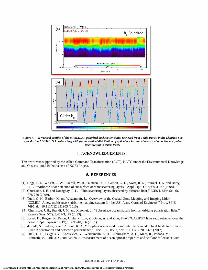
of the laser beam. Also during the cruise there were several rain storms that affect the water surface increasing its

roughness and thus contaminating the return laser waveform. Figure 4a shows an example of the retrieved Mini-

LIDAR backscattered signal during a ~2hr transit by the ship as compared to bio-optical measurements acquired in the

same general area by a Slocum glider (Fig. 4b). Both showed an elevated backscatter signal associated with biological

particles in the near surface layers down to around 20-25m.

The in-situ profiling LIDAR [Fine Structure Underwater Imaging LIDAR (FSUIL] was provided by Dr. Fraser

Dalgleish of the Harbor Branch Oceanographic Institute/Florida Atlantic University (HBOI/FAU). The FSUIL uses a

narrow collimated laser beam and a 2-axis scanner to synchronously scan a volume and simultaneously acquire two

LIDAR waveforms for each pulse. There are two detector channels; the narrow 1o FOV channel for the exponential

decay coefficient governed by the beam attenuation [c(532)] and the wider 10o FOV channel for estimating the diffuse

attenuation coefficient [K(532)]. This system was designed for observing the fine details (cm scale) of the mixing

layer or benthic boundary layer, such as turbulence and plankton/nepheloid layers. Each pulse is 40mJ at 532nm,

500ps full width at half maximum (FWHM) and 500Hz repetition rate and has the capability to observe the

backscattered returns out to 30m, depending on the water clarity and for bottoms out to over 50m in clear waters.



z(m)

0.5

Figure 3. Depth profiles of K(532) computed from the in situ optical measurements and LIDAR attenuation coefficients [a(532)]

estimated from the cross-polarized return wavefor8.

During the profiling of the FSUIL, the MASCOT (Multi-Angle Scattering and Optical Transmission, M. Twardowski)

optical package was lowered simultaneously to acquire a variety of optical measurements for comparison to the

collected LIDAR waveforms. This analysis is still progressing and results will be forthcoming in the next several

months.

3. CONCLUSIONS

This document discusses the current state-of-the-art in LIDAR research with an emphasis towards the application of

LIDAR signals for retrieving vertical profiles of the optical and physical properties in the water column. The need for

characterization and calibration (C2) is discussed as well as the novel idea of developing this LIDAR system to be

deployed above-water on ship-of-opportunity platforms. It has been shown that models exist to accurately simulate

the measured LIDAR waveforms so that the optical properties used as input into these models represent the in-situ

distribution of the properties. This area of LIDAR research has not been investigated thoroughly and this should

provide the potential for research opportunities. Future LIDAR systems for underwater communication, bathymetry,

mine detection and underwater imaging would benefit by this research as well as the physical modelers that want high

spatial and temporal resolutions of optical and physical properties for model improvement and uncertainty analyses via

data assimilation.

Future efforts should be devoted to scheduling cruises that bring together both above-water and in-situ sampling

polarized LIDAR systems. Several systems currently exist at Dr. J. Churnside’s laboratory at NOAA, USA, and also a

recently built LIDAR system that Dr. Alan Weidemman at NRL-Stennis just acquired. Another option for above-

water LIDAR measurements is to use an aircraft mounted system like the CZMIL (Coastal Zone Mapping and

Imaging LIDAR)16

by Optech Inc. that is being developed and tested under the auspices of the US Army Corps of

Engineers and the Joint Lidar Bathymetry Technical Center of Expertise. For in situ profiling LIDAR systems, Dr.

Fraser Dalgleish of HBOI/FAU could bring is FSUIL system or a new fiber-optic LIDAR17

developed at DRDC

Valcartier, CAN, by R. Gilles could be deployed.



E

a_

- 20

- 40

- 60

20130322-102409

ckSatt Polariz (Rev.1)

Sack scattered

OCO q ea

10.5 11.0Local Tme

1 I.E.' 12.0

so

i AfI

lI

03522817 00

18 0010 00

rme

220023 00

Figure 4. (a) Vertical profiles of the MiniLIDAR polarized backscatter signal retrieved from a ship transit in the Ligurian Sea

gyre during LLOMEx’13 cruise along with (b) the vertical distribution of optical backscattered measured on a Slocum glider

near the ship’s cruise track.

4. ACKNOWLEDGEMENTS

This work was supported by the Allied Command Transformation (ACT), NATO under the Environmental Knowledge

and Observational Effectiveness (EKOE) Project.

5. REFERENCES

[1] Hoge, F. E., Wright, C. W., Krabill, W. B., Buntzen, R. R., Gilbert, G. D., Swift, R. N., Yungel, J. K. and Berry,

R. E., “Airborne lidar detection of subsurface oceanic scattering layers,” Appl. Opt. 27, 3,969-3,977 (1998).

[2] Churnside, J. H. and Donaghay, P. L. “Thin scattering layers observed by airborne lidar,” ICES J. Mar. Sci. 66,

778-789 (2009). [3] Tuell, G. H., Barbor, K. and Wozencraft, J., “Overview of the Coastal Zone Mapping and Imaging Lidar

(CZMIL): A new multisensory airborne mapping system for the U.S. Army Corps of Engineers,” Proc. SPIE

7695, doi:10.1117/12.851905 (2010).

[4] Churnside, J. H., Brandi, J. M. and Xiaomei, L., “Subsurface ocean signals from an orbiting polarization lidar,”

Remote Sens. 5(7), 3,457-3,475 (2013).

[5] Josset, D., Rogers, R., Pelon, J., Hu, Y., Liu, Z., Omar, A. and Zhai, P.-W, “CALIPSO lidar ratio retrieval over the

ocean,” Opt. Express 19(19),18,696-18,706 (2011).

[6] deRada, S., Ladner, S. and Arnone, R. A., “Coupling ocean models and satellite derived optical fields to estimate

LIDAR penetration and detection performance,” Proc. SPIE 8532, doi:10.1117/12.2007323 (2012).

[7] Tuell, G. H., Feygels, V., Kopilevich, Y., Weidemann, A. D., Cunningham, A. G., Mani, R., Podoba, V.,

Ramnath, V., Park, J. Y. and Aitken, J., “Measurement of ocean optical properties and seafloor reflectance with

bb Polarized

Glider bb

(a)

(b)



Scanning Hydrographic Operational Airborne Lidar Survey (SHOALS): II Practical results and comparison with

independent data,” Proc. SPIE 5885, doi:10.1117/12.619215 (2005).

[8] Lee, J. H., Churnside, J. H., Marchbanks, R. D., Donaghay, P. L. and Sullivian, J. M, “Oceanographic lidar

profiles compared with estimates from in situ optical measurements,” Appl. Opt. 52(4), 786-794 (2013).

[9] Churnside, J. H. and Wilson, J. J., “Airborne lidar for fisheries applications,” Opt. Eng. 40, 406-414 (2001).

[9] Donia, I. S., Dolin, L. S., Levin, I. M., Rodionov, A. A. and Savel’ev, V. A., “Inverse problems of lidar sensing of

the ocean,” Pro. SPIE 6615, doi:10.1117/12.740451 (2007).

[10] Levin, I. M. and Kopelevich, O. V., “Correlations between the inherent hydroptical characteristics in the spectral

range close to 550 nm,” Mar. Phys., Oceanology 47(3), 344-349 (2007).

[11] Zege, E. P., Katsev, I. L., Prikhach, A. S. and Keeler, R. N, “Simulating the performance of airborne and in‐water

laser imaging systems,” Proc. SPIE, 4488, doi:10.1117/12.452830 (2002).

[12] Zege, E. P., Katsev, I., Prikhach, A. and Malinka, A., ”Elastic and Raman, LIDAR sounding of coastal waters.

Theory, computer simulation, inversion possibilities,” EARSel eProc. 3,2, 248- 260 (2003).

[13] Kopilevich, Y. I., Feygels, V. I., and Surkov, A., “Mathematical modeling of input signals for oceanographic

lidar systems,” Proc. SPIE 5155, doi: 10.1117/12.506980 (2003).

[14] Kopilevich, Y. I., Feygels, V. I., Tuell, G. H. and A. Surkov, A., “Measurement of ocean water optical properties

and seafloor reflectance with Scanning Hydrographic Operational Airborne Lidar Survey (SHOALS): I

Theoretical background,” Proc. SPIE 5885, doi:10.1117/12.618923 (2005).

[15] Vasilkov, A. P., Goldin, Y. A., Gureev, B. A., Hoge, F. E., Swift, R. N. and Wright, C. W., “Airborne polarized

lidar detection of scattering layers in the ocean,” Appl. Opt. 40(24), 4,353-4,364 (2001).

[16] Feygels, V. I., Park, J. Y., Wozencraft, J., Aitken, J., Macon, C., Mathur, A., Payment, A. and Ramnath, V.,

“CZMIL (coastal zone mapping and imaging lidar): from first flights to first mission through system validation,”

Proc. SPIE 87240A, doi:10.1117/12.2017935 (2013).

[17] Gilles, R., Mathieu, P., Cao, X., Cinq-Mars, A., Roy, S., Fournier, G., Marec, C. and Becu, G., “Development of

an underwater fiber-optic lidar for the characterization of sea water and ice properties,” Proc. SPIE, 8872-17

(2013).



Beyond Bathymetry: Probing the Ocean Subsurface Using Ship-Based LIDARs

Documents