TechnicalReport98-74,Dept.ofComputerScience,UniversityofMassachusetts,Amherst,MA01003.April,1998. Between MDPs and Semi-MDPs: Learning, Planning, and Representing Knowledge at Multiple Temporal Scales Richard S. Sutton [email protected] Doina Precup [email protected] University of Massachusetts, Amherst, MA 01003 USA Satinder Singh [email protected] University of Colorado, Boulder, CO 80309 USA Abstract Learning, planning, and representing knowledge at multiple levels of temporal abstrac- tion are key challenges for AI. In this paper we develop an approach to these problems based on the mathematical framework of reinforcement learning and Markov decision pro- cesses (MDPs). We extend the usual notion of action to include options —whole courses of behavior that may be temporally extended, stochastic, and contingent on events. Ex- amples of options include picking up an object, going to lunch, and traveling to a distant city, as well as primitive actions such as muscle twitches and joint torques. Options may be given a priori, learned by experience, or both. They may be used interchangeably with actions in a variety of planning and learning methods. The theory of semi-Markov decision processes (SMDPs) can be applied to model the consequences of options and as a basis for planning and learning methods using them. In this paper we develop these connections, building on prior work by Bradtke and Duff (1995), Parr (in prep.) and others. Our main novel results concern the interface between the MDP and SMDP levels of analysis. We show how a set of options can be altered by changing only their termination conditions to improve over SMDP methods with no additional cost. We also introduce intra-option temporal-difference methods that are able to learn from fragments of an option’s execution. Finally, we propose a notion of subgoal which can be used to improve the options them- selves. Overall, we argue that options and their models provide hitherto missing aspects of a powerful, clear, and expressive framework for representing and organizing knowledge. 1. Temporal Abstraction To make everyday decisions, people must foresee the consequences of their possible courses of action at multiple levels of temporal abstraction. Consider a traveler deciding to undertake a journey to a distant city. To decide whether or not to go, the benefits of the trip must be weighed against the expense. Having decided to go, choices must be made at each leg, e.g., whether to fly or to drive, whether to take a taxi or to arrange a ride. Each of these steps involves foresight and decision, all the way down to the smallest of actions. For example, just to call a taxi may involve finding a telephone, dialing each digit, and the individual muscle contractions to lift the receiver to the ear. Human decision making routinely involves

Welcome message from author
This document is posted to help you gain knowledge. Please leave a comment to let me know what you think about it! Share it to your friends and learn new things together.
Transcript
Technical!Report!98-74,!Dept.!of!Computer!Science,!University!of!Massachusetts,!Amherst,!MA!01003.!!April,!1998.
Between MDPs and Semi-MDPs:Learning, Planning, and Representing Knowledge
at Multiple Temporal Scales
Richard S. Sutton [email protected] Precup [email protected] of Massachusetts, Amherst, MA 01003 USA
Satinder Singh [email protected]
University of Colorado, Boulder, CO 80309 USA
Abstract
Learning, planning, and representing knowledge at multiple levels of temporal abstrac-tion are key challenges for AI. In this paper we develop an approach to these problemsbased on the mathematical framework of reinforcement learning and Markov decision pro-cesses (MDPs). We extend the usual notion of action to include options—whole coursesof behavior that may be temporally extended, stochastic, and contingent on events. Ex-amples of options include picking up an object, going to lunch, and traveling to a distantcity, as well as primitive actions such as muscle twitches and joint torques. Options maybe given a priori, learned by experience, or both. They may be used interchangeably withactions in a variety of planning and learning methods. The theory of semi-Markov decisionprocesses (SMDPs) can be applied to model the consequences of options and as a basis forplanning and learning methods using them. In this paper we develop these connections,building on prior work by Bradtke and Du! (1995), Parr (in prep.) and others. Our mainnovel results concern the interface between the MDP and SMDP levels of analysis. Weshow how a set of options can be altered by changing only their termination conditionsto improve over SMDP methods with no additional cost. We also introduce intra-optiontemporal-di!erence methods that are able to learn from fragments of an option’s execution.Finally, we propose a notion of subgoal which can be used to improve the options them-selves. Overall, we argue that options and their models provide hitherto missing aspects ofa powerful, clear, and expressive framework for representing and organizing knowledge.
1. Temporal Abstraction
To make everyday decisions, people must foresee the consequences of their possible courses ofaction at multiple levels of temporal abstraction. Consider a traveler deciding to undertakea journey to a distant city. To decide whether or not to go, the benefits of the trip must beweighed against the expense. Having decided to go, choices must be made at each leg, e.g.,whether to fly or to drive, whether to take a taxi or to arrange a ride. Each of these stepsinvolves foresight and decision, all the way down to the smallest of actions. For example,just to call a taxi may involve finding a telephone, dialing each digit, and the individualmuscle contractions to lift the receiver to the ear. Human decision making routinely involves
Sutton, Precup, & Singh
planning and foresight—choice among temporally-extended options—over a broad range oftime scales.
In this paper we examine the nature of the knowledge needed to plan and learn atmultiple levels of temporal abstraction. The principal knowledge needed is the ability topredict the consequences of di!erent courses of action. This may seem straightforward, butit is not. It is not at all clear what we mean either by a “course of action” or, particularly, by“its consequences”. One problem is that most courses of action have many consequences,with the immediate consequences di!erent from the longer-term ones. For example, thecourse of action go-to-the-librarymay have the near-term consequence of being outdoorsand walking, and the long-term consequence of being indoors and reading. In addition, weusually only consider courses of action for a limited but indefinite time period. An actionlike wash-the-car is most usefully executed up until the car is clean, but without specifyinga particular time at which it is to stop. We seek a way of representing predictive knowledgethat is:
Expressive The representation must be able to include basic kinds of commonsense knowl-edge such as the examples we have mentioned. In particular, it should be able to pre-dict consequences that are temporally extended and uncertain. This criterion rulesout many conventional engineering representations, such as di!erential equations andtransition probabilities. The representation should also be able to predict the con-sequences of courses of action that are stochastic and contingent on subsequent ob-servations. This rules out simple sequences of action with a deterministically knownoutcome, such as conventional macro-operators.
Clear The representation should be clear, explicit, and grounded in primitive observationsand actions. Ideally it would be expressed in a formal mathematical language. Anypredictions made should be testable simply by comparing them against data: nohuman interpretation should be necessary. This criterion rules out conventional AIrepresentations with ungrounded symbols. For example, “Tweety is a bird” relieson people to understand “Tweety,” “Bird,” and “is-a”; none of these has a clearinterpretation in terms of observables. A related criterion is that the representationshould be learnable. Only a representation that is clear and directly testable fromobservables is likely to be learnable. A clear representation need not be unambiguous.For example, it could predict that one of two events will occur at a particular time,but not specify which of them will occur.
Suitable for Planning A representation of knowledge must be suitable for how it willbe used as part of planning and decision-making. In particular, the representationshould enable interrelating and intermixing knowledge at di!erent levels of temporalabstraction.
It should be clear that we are addressing a fundamental question of AI: how shouldan intelligent agent represent its knowledge of the world? We are interested here in theunderlying semantics of the knowledge, not with its surface form. In particular, we arenot concerned with the data structures of the knowledge representation, e.g., whether the
2
Between MDPs and Semi-MDPs
knowledge is represented by neural networks or symbolic rules. Whatever data structuresare used to generate the predictions, our concern is with their meaning, i.e., with theinterpretation that we or that other parts of the system can make of the predictions. Isthe meaning clear and grounded enough to be tested and learned? Do the representablemeanings include the commonsense predictions we seem to use in everyday planning? Arethese meanings su"cient to support e!ective planning?
Planning with temporally extended actions has been extensively explored in severalfields. Early AI research focused on it from the point of view of abstraction in planning(e.g., Fikes, Hart, and Nilsson, 1972; Newell and Simon, 1972; Nilsson, 1973; Sacerdoti,1974). More recently, macro-operators, qualitative modeling, and other ways of chunkingaction selections into units have been extensively developed (e.g., Kuipers, 1979; de Kleerand Brown, 1984; Korf, 1985, 1987; Laird, Rosenbloom and Newell, 1986; Minton, 1988;Iba, 1989; Drescher, 1991; Ruby and Kibler, 1992; Dejong, 1994; Levinson and Fuchs, 1994;Nilsson, 1994; Say and Selahattin, 1996; Brafman and Moshe, 1997; Haigh, Shewchuk, andVeloso, 1997). Roboticists and control engineers have long considered methodologies forcombining and switching between independently designed controllers (e.g., Brooks, 1986;Maes, 1991; Koza and Rice, 1992; Brockett, 1993; Grossman et al., 1993; Millan, 1994;Araujo and Grupen, 1996; Colombetti, Dorigo, and Borghi, 1996; Dorigo and Colombetti,1994; Toth, Kovacs, and Lorincz, 1995; Sastry, 1997; Rosenstein and Cohen, 1998). Morerecently, the topic has been taken up within the framework of MDPs and reinforcementlearning (Watkins, 1989; Ring, 1991; Wixson, 1991; Schmidhuber, 1991; Mahadevan andConnell, 1992; Tenenberg, Karlsson, and Whitehead, 1992; Lin, 1993; Dayan and Hinton,1993; Dayan, 1993; Kaelbling, 1993; Singh et al., 1994; Chrisman, 1994; Hansen, 1994;Uchibe, Asada and Hosada, 1996; Asada et al., 1996; Thrun and Schwartz, 1995; Kalmar,Szepesvari, and Lorincz, 1997, in prep.; Dietterich, 1997; Mataric, 1997; Huber and Gru-pen, 1997; Wiering and Schmidhuber, 1997; Parr and Russell, 1998; Drummond, 1998;Hauskrecht et al., in prep.; Meuleau, in prep.), within which we also work here. Our re-cent work in this area (Precup and Sutton, 1997, 1998; Precup, Sutton, and Singh, 1997,1998; see also McGovern, Sutton, and Fagg, 1997; McGovern and Sutton, in prep.) can beviewed as a combination and generalization of Singh’s hierarchical Dyna (1992a,b,c,d) andSutton’s mixture models (1995; Sutton and Pinette, 1985). In the current paper we simplifyour treatment of the ideas by linking temporal abstraction to the theory of Semi-MDPs, asin Parr (in prep.), and as we discuss next.
2. Between MDPs and SMDPs
In this paper we explore the extent to which Markov decision processes (MDPs) can providea mathematical foundation for the study of temporal abstraction and temporally extendedaction. MDPs have been widely used in AI in recent years to study planning and learning instochastic environments (e.g., Barto, Bradtke, and Singh, 1995; Dean et al., 1995; Boutilier,Brafman, and Gelb, 1997; Simmons and Koenig, 1995; Ge!ner and Bonet, in prep.). Theyprovide a simple formulation of the AI problem including sensation, action, stochastic cause-and-e!ect, and general goals formulated as reward signals. E!ective learning and planningmethods for MDPs have been proven in a number of significant applications (e.g., Mahade-
3
Sutton, Precup, & Singh
MDP
SMDP
Options
over MDP
State
Time
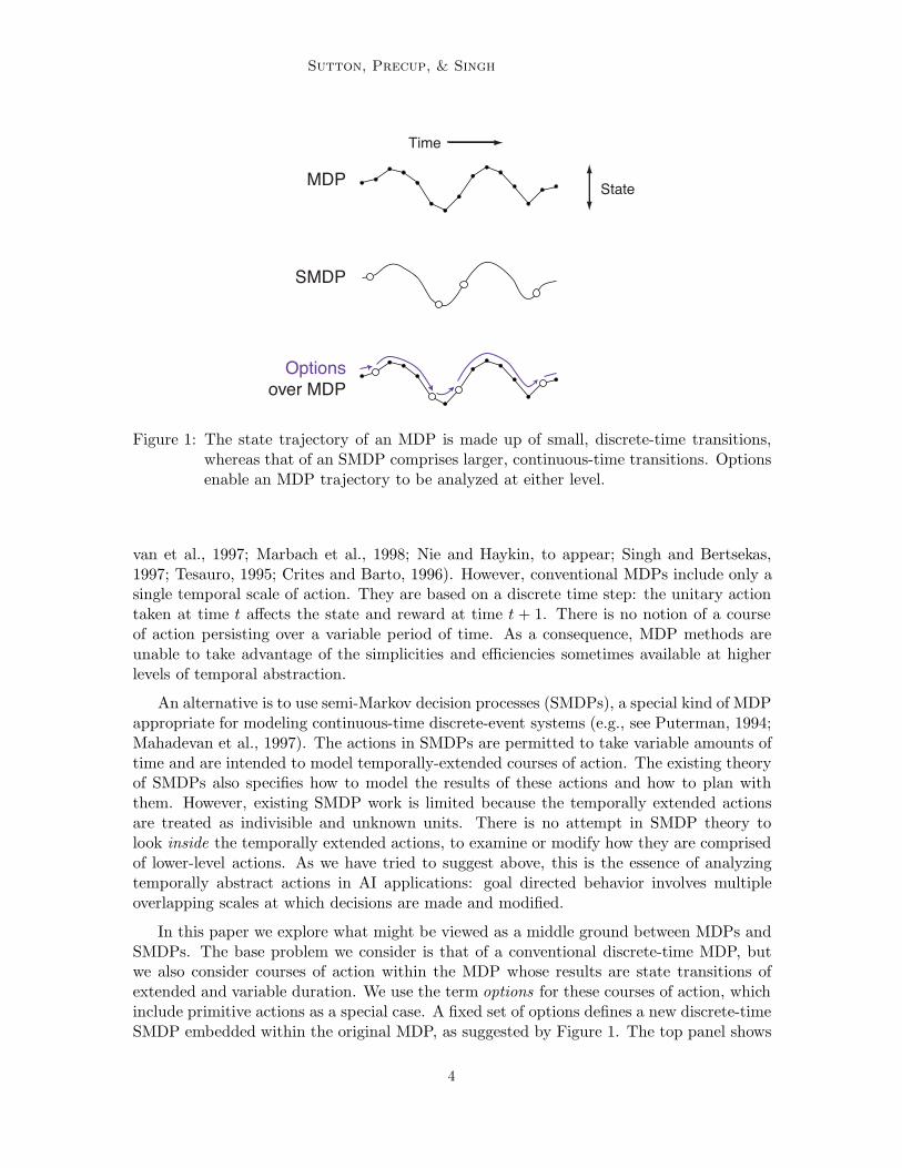
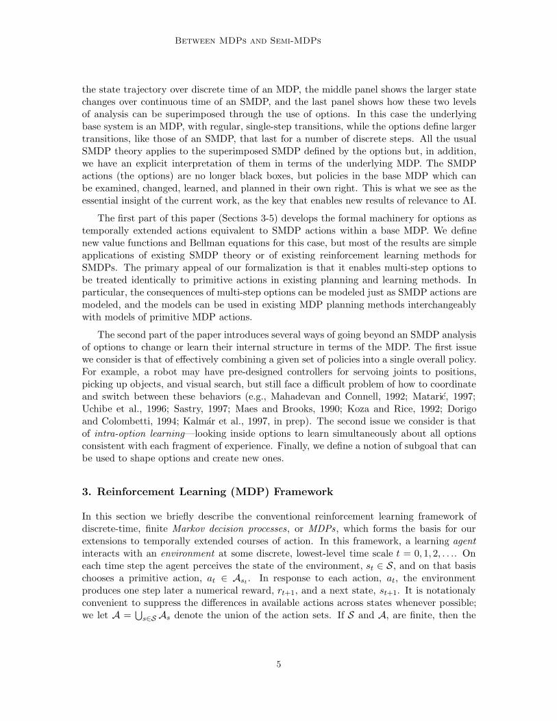
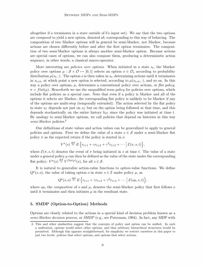
Figure 1: The state trajectory of an MDP is made up of small, discrete-time transitions,whereas that of an SMDP comprises larger, continuous-time transitions. Optionsenable an MDP trajectory to be analyzed at either level.
van et al., 1997; Marbach et al., 1998; Nie and Haykin, to appear; Singh and Bertsekas,1997; Tesauro, 1995; Crites and Barto, 1996). However, conventional MDPs include only asingle temporal scale of action. They are based on a discrete time step: the unitary actiontaken at time t a!ects the state and reward at time t + 1. There is no notion of a courseof action persisting over a variable period of time. As a consequence, MDP methods areunable to take advantage of the simplicities and e"ciencies sometimes available at higherlevels of temporal abstraction.
An alternative is to use semi-Markov decision processes (SMDPs), a special kind of MDPappropriate for modeling continuous-time discrete-event systems (e.g., see Puterman, 1994;Mahadevan et al., 1997). The actions in SMDPs are permitted to take variable amounts oftime and are intended to model temporally-extended courses of action. The existing theoryof SMDPs also specifies how to model the results of these actions and how to plan withthem. However, existing SMDP work is limited because the temporally extended actionsare treated as indivisible and unknown units. There is no attempt in SMDP theory tolook inside the temporally extended actions, to examine or modify how they are comprisedof lower-level actions. As we have tried to suggest above, this is the essence of analyzingtemporally abstract actions in AI applications: goal directed behavior involves multipleoverlapping scales at which decisions are made and modified.
In this paper we explore what might be viewed as a middle ground between MDPs andSMDPs. The base problem we consider is that of a conventional discrete-time MDP, butwe also consider courses of action within the MDP whose results are state transitions ofextended and variable duration. We use the term options for these courses of action, whichinclude primitive actions as a special case. A fixed set of options defines a new discrete-timeSMDP embedded within the original MDP, as suggested by Figure 1. The top panel shows
4
Between MDPs and Semi-MDPs
the state trajectory over discrete time of an MDP, the middle panel shows the larger statechanges over continuous time of an SMDP, and the last panel shows how these two levelsof analysis can be superimposed through the use of options. In this case the underlyingbase system is an MDP, with regular, single-step transitions, while the options define largertransitions, like those of an SMDP, that last for a number of discrete steps. All the usualSMDP theory applies to the superimposed SMDP defined by the options but, in addition,we have an explicit interpretation of them in terms of the underlying MDP. The SMDPactions (the options) are no longer black boxes, but policies in the base MDP which canbe examined, changed, learned, and planned in their own right. This is what we see as theessential insight of the current work, as the key that enables new results of relevance to AI.
The first part of this paper (Sections 3-5) develops the formal machinery for options astemporally extended actions equivalent to SMDP actions within a base MDP. We definenew value functions and Bellman equations for this case, but most of the results are simpleapplications of existing SMDP theory or of existing reinforcement learning methods forSMDPs. The primary appeal of our formalization is that it enables multi-step options tobe treated identically to primitive actions in existing planning and learning methods. Inparticular, the consequences of multi-step options can be modeled just as SMDP actions aremodeled, and the models can be used in existing MDP planning methods interchangeablywith models of primitive MDP actions.
The second part of the paper introduces several ways of going beyond an SMDP analysisof options to change or learn their internal structure in terms of the MDP. The first issuewe consider is that of e!ectively combining a given set of policies into a single overall policy.For example, a robot may have pre-designed controllers for servoing joints to positions,picking up objects, and visual search, but still face a di"cult problem of how to coordinateand switch between these behaviors (e.g., Mahadevan and Connell, 1992; Mataric, 1997;Uchibe et al., 1996; Sastry, 1997; Maes and Brooks, 1990; Koza and Rice, 1992; Dorigoand Colombetti, 1994; Kalmar et al., 1997, in prep). The second issue we consider is thatof intra-option learning—looking inside options to learn simultaneously about all optionsconsistent with each fragment of experience. Finally, we define a notion of subgoal that canbe used to shape options and create new ones.
3. Reinforcement Learning (MDP) Framework
In this section we briefly describe the conventional reinforcement learning framework ofdiscrete-time, finite Markov decision processes, or MDPs, which forms the basis for ourextensions to temporally extended courses of action. In this framework, a learning agentinteracts with an environment at some discrete, lowest-level time scale t = 0, 1, 2, . . .. Oneach time step the agent perceives the state of the environment, st ! S, and on that basischooses a primitive action, at ! Ast . In response to each action, at, the environmentproduces one step later a numerical reward, rt+1, and a next state, st+1. It is notationalyconvenient to suppress the di!erences in available actions across states whenever possible;we let A =
!s!S As denote the union of the action sets. If S and A, are finite, then the
5
Sutton, Precup, & Singh
environment’s transition dynamics are modeled by one-step state-transition probabilities,
pass! = Pr
"st+1 = s" | st = s, at = a
#,
and one-step expected rewards,
ras = E{rt+1 | st = s, at = a},
for all s, s" ! S and a ! A (it is understood here that pass! = 0 for a "! As). These two sets
of quantities together constitute the one-step model of the environment.
The agent’s objective is to learn an optimal Markov policy, a mapping from states toprobabilities of taking each available primitive action, ! : S # A $% [0, 1], that maximizesthe expected discounted future reward from each state s:
V !(s) = E$rt+1 + "rt+1 + "2rt+1 + · · ·
%%% st = s,!&
(1)
= E$rt+1 + "V !(st+1)
%%% st = s,!&
='
a!As
!(s, a)(
ras + "
'
s!pa
ss!V!(s")
)
, (2)
where !(s, a) is the probability with which the policy ! chooses action a ! As in state s,and " ! [0, 1] is a discount-rate parameter. This quantity, V !(s), is called the value of states under policy !, and V ! is called the state-value function for !. The optimal state-valuefunction gives the value of a state under an optimal policy:
V #(s) = max!
V !(s) (3)
= maxa!As
E$rt+1 + "V #(st+1)
%%% st = s, at = a&
= maxa!As
(
ras + "
'
s!pa
ss!V#(s")
)
. (4)
Any policy that achieves the maximum in (3) is by definition an optimal policy. Thus,given V #, an optimal policy is easily formed by choosing in each state s any action thatachieves the maximum in (4). Planning in reinforcement learning refers to the use ofmodels of the environment to compute value functions and thereby to optimize or improvepolicies. Particularly useful in this regard are Bellman equations, such as (2) and (4), whichrecursively relate value functions to themselves. If we treat the values, V !(s) or V #(s), asunknowns, then a set of Bellman equations, for all s ! S, forms a system of equations whoseunique solution is in fact V ! or V # as given by (1) or (3). This fact is key to the way inwhich all temporal-di!erence and dynamic programming methods estimate value functions.
Particularly important for learning methods is a parallel set of value functions andBellman equations for state–action pairs rather than for states. The value of taking actiona in state s under policy !, denoted Q!(s, a), is the expected discounted future rewardstarting in s, taking a, and henceforth following !:
Q!(s, a) = E$rt+1 + "rt+1 + "2rt+1 + · · ·
%%% st = s, at = a,!&
6
Between MDPs and Semi-MDPs
= ras + "
'
s!pa
ss!V!(s")
= ras + "
'
s!pa
ss!'
a!!(s, a")Q!(s", a").
This is known as the action-value function for policy !. The optimal action-value functionis
Q#(s, a) = max!
Q!(s, a)
= ras + "
'
s!pa
ss! maxa!
Q#(s", a").
Finally, many tasks are episodic in nature, involving repeated trials, or episodes, eachending with a reset to a standard state or state distribution. In these episodic tasks, weinclude a single special terminal state, arrival in which terminates the current episode. Theset of regular states plus the terminal state (if there is one) is denoted S+. Thus, the s" inpa
ss! in general ranges over the set S+ rather than just S as stated earlier. In an episodictask, values are defined by the expected cumulative reward up until termination rather thanover the infinite future (or, equivalently, we can consider the terminal state to transition toitself forever with a reward of zero).
4. Options
We use the term options for our generalization of primitive actions to include temporallyextended courses of action. Options consist of three components: a policy ! : S#A $% [0, 1],a termination condition # : S+ $% [0, 1], and an input set I & S. An option 'I,!,#( isavailable in state s if and only if s ! I. If the option is taken, then actions are selectedaccording to ! until the option terminates stochastically according to #. In particular, if theoption taken in state st is Markov , then the next action at is selected according to the prob-ability distribution !(s, ·). The environment then makes a transition to state st+1, wherethe option either terminates, with probability #(st+1), or else continues, determining at+1
according to !(st+1, ·), possibly terminating in st+2 according to #(st+2), and so on.1 Whenthe option terminates, then the agent has the opportunity to select another option. Forexample, an option named open-the-door might consist of a policy for reaching, graspingand turning the door knob, a termination condition for recognizing that the door has beenopened, and an input set restricting consideration of open-the-door to states in which adoor is present. In episodic tasks, termination of an episode also terminates the currentoption (i.e., # maps the terminal state to 1 in all options).
The input set and termination condition of an option together restrict its range ofapplication in a potentially useful way. In particular, they limit the range over which theoption’s policy need be defined. For example, a handcrafted policy ! for a mobile robot todock with its battery charger might be defined only for states I in which the battery charger
1. The termination condition ! plays a role similar to the ! in !-models (Sutton, 1995), but with anopposite sense. That is, !(s) in this paper corresponds to 1 ! !(s) in that earlier paper.
7
Sutton, Precup, & Singh
is within sight. The termination condition # could be defined to be 1 outside of I and whenthe robot is successfully docked. A subpolicy for servoing a robot arm to a particular jointconfiguration could similarly have a set of allowed starting states, a controller to be appliedto them, and a termination condition indicating that either the target configuration hadbeen reached within some tolerance or that some unexpected event had taken the subpolicyoutside its domain of application. For Markov options it is natural to assume that all stateswhere an option might continue are also states where the option might be taken (i.e., that{s : #(s) < 1} &I ). In this case, ! need only be defined over I rather than over all of S.
Sometimes it is useful for options to “timeout,” to terminate after some period of timehas elapsed even if they have failed to reach any particular state. Unfortunately, this isnot possible with Markov options because their termination decisions are made solely onthe basis of the current state, not on how long the option has been executing. To handlethis and other cases of interest we consider a generalization to semi-Markov options, inwhich policies and termination conditions may make their choices dependent on all priorevents since the option was initiated. In general, an option is initiated at some time, sayt, determines the actions selected for some number of steps, say k, and then terminatesin st+k. At each intermediate time T , t ) T < t + k, the decisions of a Markov optionmay depend only on sT , whereas the decisions of a semi-Markov option may depend on theentire sequence st, at, rt+1, st+1, at+1, . . . , rT , sT , but not on events prior to st (or after sT ).We call this sequence the history from t to T and denote it by htT . We denote the set of allhistories by #. In semi-Markov options, the policy and termination condition are functionsof possible histories, that is, they are ! : ##A $% [0, 1] and # : # $% [0, 1]. The semi-Markovcase is also useful for cases in which options use a more detailed state representation thanis available to the policy that selects the options.
Given a set of options, their input sets implicitly define a set of available options Os
for each state s ! S. These Os are much like the sets of available actions, As. We canunify these two kinds of sets by noting that actions can be considered a special case ofoptions. Each action a corresponds to an option that is available whenever a is available(I = {s : a ! As}), that always lasts exactly one step (#(s) = 1, *s ! S), and that selectsa everywhere (!(s, a) = 1, *s ! I). Thus, we can consider the agent’s choice at each timeto be entirely among options, some of which persist for a single time step, others which aremore temporally extended. The former we refer to as one-step or primitive options and thelatter as multi-step options. Just as in the case of actions, it is convenient to notationalysuppress the di!erences in available options across states. We let O =
!s!S Os denote the
set of all available options.
Our definition of options is crafted to make them as much like actions as possible,except temporally extended. Because options terminate in a well defined way, we canconsider sequences of them in much the same way as we consider sequences of actions. Wecan consider policies that select options instead of primitive actions, and we can modelthe consequences of selecting an option much as we model the results of an action. Let usconsider each of these in turn.
Given any two options a and b, we can consider taking them in sequence, that is, wecan consider first taking a until it terminates, and then b until it terminates (or omitting b
8
Between MDPs and Semi-MDPs
altogether if a terminates in a state outside of b’s input set). We say that the two optionsare composed to yield a new option, denoted ab, corresponding to this way of behaving. Thecomposition of two Markov options will in general be semi-Markov, not Markov, becauseactions are chosen di!erently before and after the first option terminates. The composi-tion of two semi-Markov options is always another semi-Markov option. Because actionsare special cases of options, we can also compose them, producing a deterministic actionsequence, in other words, a classical macro-operator.
More interesting are policies over options. When initiated in a state st, the Markovpolicy over options µ : S # O $% [0, 1] selects an option o ! Os according to probabilitydistribution µ(st, ·). The option o is then taken in st, determining actions until it terminatesin st+k, at which point a new option is selected, according to µ(st+k, ·), and so on. In thisway a policy over options, µ, determines a conventional policy over actions, or flat policy,! = flat(µ). Henceforth we use the unqualified term policy for policies over options, whichinclude flat policies as a special case. Note that even if a policy is Markov and all of theoptions it selects are Markov, the corresponding flat policy is unlikely to be Markov if anyof the options are multi-step (temporally extended). The action selected by the flat policyin state sT depends not just on sT but on the option being followed at that time, and thisdepends stochastically on the entire history htT since the policy was initiated at time t.By analogy to semi-Markov options, we call policies that depend on histories in this waysemi-Markov policies.2
Our definitions of state values and action values can be generalized to apply to generalpolicies and options. First we define the value of a state s ! S under a semi-Markov flatpolicy ! as the expected return if the policy is started in s:
V !(s) def= E$rt+1 + "rt+2 + "2rt+3 + · · ·
%%% E(!, s, t)&,
where E(!, s, t) denotes the event of ! being initiated in s at time t. The value of a stateunder a general policy µ can then be defined as the value of the state under the correspondingflat policy: V µ(s) def= V flat(µ)(s), for all s ! S.
It is natural to generalize action-value functions to option-value functions. We defineQµ(s, o), the value of taking option o in state s ! I under policy µ, as
Qµ(s, o) def= E$rt+1 + "rt+2 + "2rt+3 + · · ·
%%% E(oµ, s, t)&,
where oµ, the composition of o and µ, denotes the semi-Markov policy that first follows ountil it terminates and then initiates µ in the resultant state.
5. SMDP (Option-to-Option) Methods
Options are closely related to the actions in a special kind of decision problem known as asemi-Markov decision process, or SMDP (e.g., see Puterman, 1994). In fact, any MDP with
2. This and other similarities suggest that the concepts of policy and option can be unified. In sucha unification, options would select other options, and thus arbitrary hierarchical structures would bepermitted. Although this appears straightforward, for simplicity we restrict ourselves in this paper tojust two levels: policies that select options, and options that select actions.
9
Sutton, Precup, & Singh
a fixed set of options is an SMDP, as we state formally below. This theorem is not really aresult, but a simple observation that follows more or less immediately from definitions. Wepresent it as a theorem to highlight it and state explicitly its conditions and consequences:
Theorem 1 (MDP + Options = SMDP) For any MDP, and any set of options de-fined on that MDP, the decision process that selects among those options, executing each totermination, is an SMDP.
Proof: (Sketch) An SMDP consists of 1) a set of states, 2) a set of actions, 3) for eachpair of state and action, an expected cumulative discounted reward, and 4) a well-definedjoint distribution of the next state and transit time. In our case, the set of states is S, andthe set of actions is just the set of options. The expected reward and the next-state andtransit-time distributions are defined for each state and option by the MDP and by theoption’s policy and termination condition, ! and #. These expectations and distributionsare well defined because the MDP is Markov and the options are semi-Markov; thus thenext state, reward, and time are dependent only on the option and the state in which itwas initiated. The transit times of options are always discrete, but this is simply a specialcase of the arbitrary real intervals permitted in SMDPs. +
The relationship between MDPs, options, and SMDPs provides a basis for the theory ofplanning and learning methods with options. In later sections we discuss the limitations ofthis theory due to its treatment of options as indivisible units without internal structure,but in this section we focus on establishing the benefits and assurances that it provides. Weestablish theoretical foundations and then survey SMDP methods for planning and learningwith options. Although our formalism is slightly di!erent, these results are in essence takenor adapted from prior work (including classical SMDP work and Singh, 1992a,b,c,d; Bradtkeand Du!, 1995; Sutton, 1995; Precup and Sutton, 1997, 1998; Precup, Sutton, and Singh,1997, 1998; Parr and Russell, 1998; McGovern, Sutton, and Fagg, 1997; Parr, in prep.). Aresult very similar to Theorem 1 was proved in detail by Parr (in prep.). In the sectionsfollowing this one we present new methods that improve over SMDP methods.
Planning with options requires a model of their consequences. Fortunately, the appro-priate form of model for options, analogous to the ra
s and pass! defined earlier for actions, is
known from existing SMDP theory. For each state in which an option may be started, thiskind of model predicts the state in which the option will terminate and the total rewardreceived along the way. These quantities are discounted in a particular way. For any optiono, let E(o, s, t) denote the event of o being initiated in state s at time t. Then the rewardpart of the model of o for any state s ! S is
ros = E
$rt+1 + "rt+2 + · · · + "k$1rt+k
%%% E(o, s, t)&, (5)
where t + k is the random time at which o terminates. The state-prediction part of themodel of o for state s is
poss! =
%'
j=1
"j Pr"st+k = s", k = j | E(o, s, t)
#
= E$"k$s!st+k
| E(o, s, t)&, (6)
10
Between MDPs and Semi-MDPs
for all s" ! S, under the same conditions, where $ss! is an identity indicator, equal to 1 ifs = s", and equal to 0 otherwise. Thus, po
ss! is a combination of the likelihood that s" isthe state in which o terminates together with a measure of how delayed that outcome isrelative to ". We call this kind of model a multi-time model (Precup and Sutton, 1997,1998) because it describes the outcome of an option not at a single time but at potentiallymany di!erent times, appropriately combined.3
Using multi-time models we can write Bellman equations for general policies and options.For any Markov policy µ, the state-value function can be written
V µ(s) = E$rt+1 + · · · + "k$1rt+k + "kV µ(st+k)
%%% E(µ, s, t)&,
where k is the duration of the first option selected by µ,
='
o!Os
µ(s, o)(
ros +
'
s!po
ss!Vµ(s")
)
, (7)
which is a Bellman equation analogous to (2). The corresponding Bellman equation for thevalue of an option o in state s ! I is
Qµ(s, o) = E$rt+1 + · · · + "k$1rt+k + "kV µ(st+k)
%%% E(o, s, t)&
= E$rt+1 + · · · + "k$1rt+k + "k
'
o!!Os
µ(st+k, o")Qµ(st+k, o
")%%% E(o, s, t)
&
= ros +
'
s!po
ss!'
o!!Os
µ(s", o")Qµ(s", o"). (8)
Note that all these equations specialize to those given earlier in the special case in which µis a conventional policy and o is a conventional action. Also note that Qµ(s, o) = V oµ(s).
Finally, there are generalizations of optimal value functions and optimal Bellman equa-tions to options and to policies over options. Of course the conventional optimal valuefunctions V # and Q# are not a!ected by the introduction of options; one can ultimately dojust as well with primitive actions as one can with options. Nevertheless, it is interestingto know how well one can do with a restricted set of options that does not include all theactions. For example, in planning one might first consider only high-level options in orderto find an approximate plan quickly. Let us denote the restricted set of options by O andthe set of all policies selecting only from options in O by $(O). Then the optimal valuefunction given that we can select only from O is
V #O(s) def= max
µ!"(O)V µ(s)
= maxo!Os
E$rt+1 + · · · + "k$1rt+k + "kV #
O(st+k)%%% E(o, s, t)
&,
where k is the duration of o when taken in st,
3. Note that the definition of state predictions in multi-time models di!ers slightly from that given earlierfor primitive actions. Under the new definition, the model of transition from state s to s! for primitiveaction a is not simply the corresponding transition probability, but the transition probability times ".Henceforth we use the new definition given by (6).
11
Sutton, Precup, & Singh
= maxo!Os
(
ros +
'
s!po
ss!V#O(s")
)
(9)
= maxo!Os
E$r + "kV #
O(s")%%% E(o, s)
&, (10)
where E(o, s) denotes option o being initiated in state s. Conditional on this event are theusual random variables: s" is the state in which o terminates, r is the cumulative discountedreward along the way, and k is the number of time steps elapsing between s and s". Thevalue functions and Bellman equations for optimal option values are
Q#O(s, o) def= max
µ!"(O)Qµ(s, o)
= E$rt+1 + · · · + "k$1rt+k + "kV #
O(st+k)%%% E(o, s, t)
&,
where k is the duration of o from st,= E
$rt+1 + · · · + "k$1rt+k + "k max
o!!Ost+k
Q#O(st+k, o
")%%% E(o, s, t)
&,
= ros +
'
s!po
ss! maxo!!Ost+k
Q#O(s", o") (11)
= E$r + "k max
o!!Ost+k
Q#O(s", o")
%%% E(o, s)&,
where r, k, and s" are again the reward, number of steps, and next state due to takingo ! Os.
Given a set of options, O, a corresponding optimal policy, denoted µ#O, is any policy
that achieves V #O, i.e., for which V µ"
O(s) = V #O(s) in all states s ! S. If V #
O and models ofthe options are known, then optimal policies can be formed by choosing in any proportionamong the maximizing options in (9) or (10). Or, if Q#
O is known, then optimal policies canbe found without a model by choosing in each state s in any proportion among the optionso for which Q#
O(s, o) = maxo! Q#O(s, o"). In this way, computing approximations to V #
O orQ#
O become key goals of planning and learning methods with options.
5.1 SMDP Planning
With these definitions, an MDP together with the set of options O formally comprises anSMDP, and standard SMDP methods and results apply. Each of the Bellman equationsfor options, (7), (8), (9), and (11), defines a system of equations whose unique solution isthe corresponding value function. These Bellman equations can be used as update rulesin dynamic-programming-like planning methods for finding the value functions. Typically,solution methods for this problem maintain an approximation of V #
O(s) or Q#O(s, o) for all
states s ! S and all options o ! Os. For example, synchronous value iteration (SVI) withoptions initializes an approximate value function V0(s) arbitrarily and then updates it by
Vk+1(s) , maxo!Os
*
+ros +
'
s!!S+
poss!Vk(s")
,
- (12)
12
Between MDPs and Semi-MDPs
o%
HALLWAYS
o&
8 multi-step options
up
down
rightleft
(to each room’s 2 hallways)
G%
4 stochastic primitive actions
Fail 33% of the time
G&
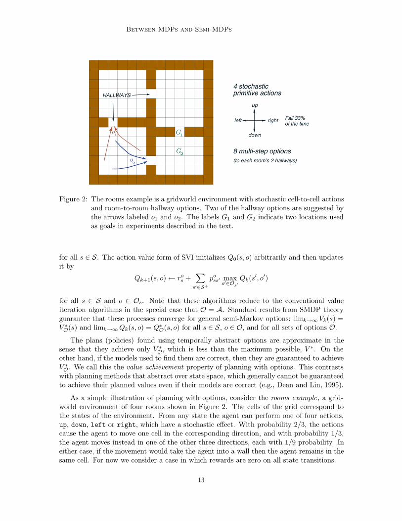
Figure 2: The rooms example is a gridworld environment with stochastic cell-to-cell actionsand room-to-room hallway options. Two of the hallway options are suggested bythe arrows labeled o1 and o2. The labels G1 and G2 indicate two locations usedas goals in experiments described in the text.
for all s ! S. The action-value form of SVI initializes Q0(s, o) arbitrarily and then updatesit by
Qk+1(s, o) , ros +
'
s!!S+
poss! max
o!!Os!Qk(s", o")
for all s ! S and o ! Os. Note that these algorithms reduce to the conventional valueiteration algorithms in the special case that O = A. Standard results from SMDP theoryguarantee that these processes converge for general semi-Markov options: limk&% Vk(s) =V #O(s) and limk&% Qk(s, o) = Q#
O(s, o) for all s ! S, o ! O, and for all sets of options O.
The plans (policies) found using temporally abstract options are approximate in thesense that they achieve only V #
O, which is less than the maximum possible, V #. On theother hand, if the models used to find them are correct, then they are guaranteed to achieveV #O. We call this the value achievement property of planning with options. This contrasts
with planning methods that abstract over state space, which generally cannot be guaranteedto achieve their planned values even if their models are correct (e.g., Dean and Lin, 1995).
As a simple illustration of planning with options, consider the rooms example, a grid-world environment of four rooms shown in Figure 2. The cells of the grid correspond tothe states of the environment. From any state the agent can perform one of four actions,up, down, left or right, which have a stochastic e!ect. With probability 2/3, the actionscause the agent to move one cell in the corresponding direction, and with probability 1/3,the agent moves instead in one of the other three directions, each with 1/9 probability. Ineither case, if the movement would take the agent into a wall then the agent remains in thesame cell. For now we consider a case in which rewards are zero on all state transitions.
13
Sutton, Precup, & Singh
Target
Hallway
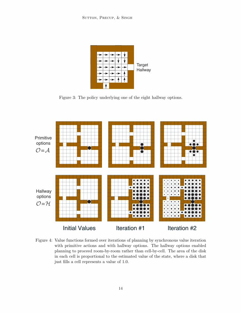
Figure 3: The policy underlying one of the eight hallway options.
Iteration #1Initial Values Iteration #2
O=A
Primitiveoptions
O=H
Hallwayoptions
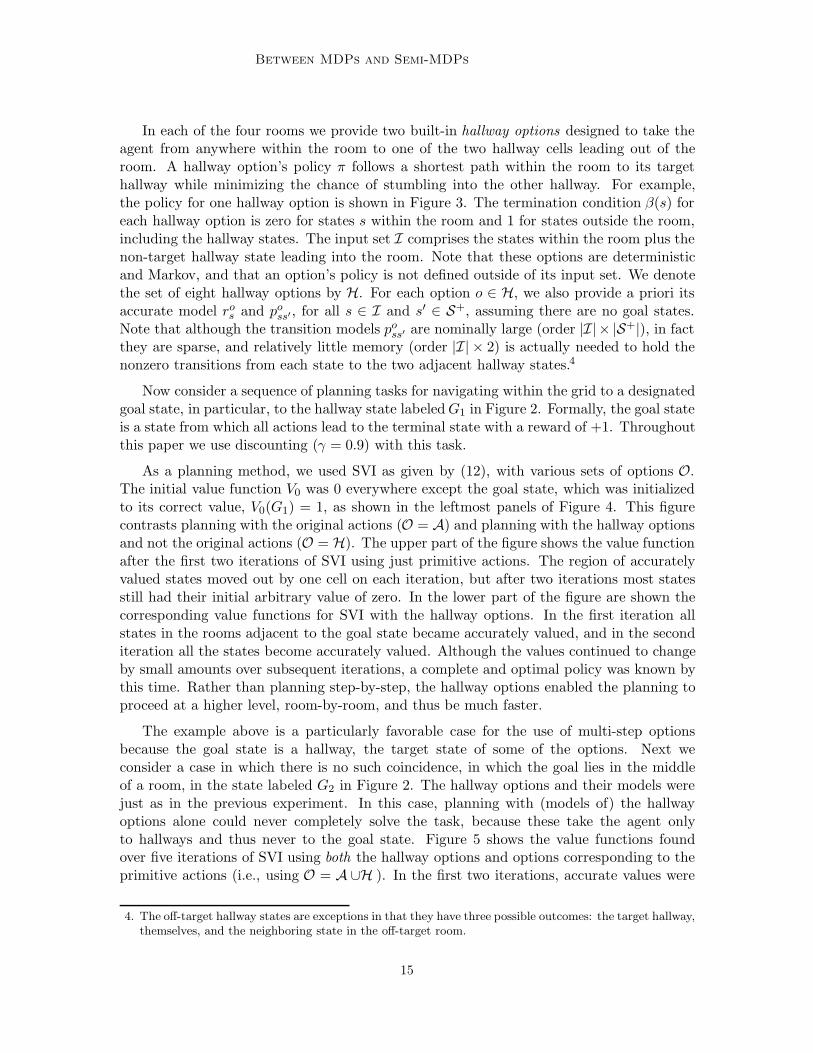
Figure 4: Value functions formed over iterations of planning by synchronous value iterationwith primitive actions and with hallway options. The hallway options enabledplanning to proceed room-by-room rather than cell-by-cell. The area of the diskin each cell is proportional to the estimated value of the state, where a disk thatjust fills a cell represents a value of 1.0.
14
Between MDPs and Semi-MDPs
In each of the four rooms we provide two built-in hallway options designed to take theagent from anywhere within the room to one of the two hallway cells leading out of theroom. A hallway option’s policy ! follows a shortest path within the room to its targethallway while minimizing the chance of stumbling into the other hallway. For example,the policy for one hallway option is shown in Figure 3. The termination condition #(s) foreach hallway option is zero for states s within the room and 1 for states outside the room,including the hallway states. The input set I comprises the states within the room plus thenon-target hallway state leading into the room. Note that these options are deterministicand Markov, and that an option’s policy is not defined outside of its input set. We denotethe set of eight hallway options by H. For each option o ! H, we also provide a priori itsaccurate model ro
s and poss! , for all s ! I and s" ! S+, assuming there are no goal states.
Note that although the transition models poss! are nominally large (order |I|# |S+|), in fact
they are sparse, and relatively little memory (order |I|# 2) is actually needed to hold thenonzero transitions from each state to the two adjacent hallway states.4
Now consider a sequence of planning tasks for navigating within the grid to a designatedgoal state, in particular, to the hallway state labeled G1 in Figure 2. Formally, the goal stateis a state from which all actions lead to the terminal state with a reward of +1. Throughoutthis paper we use discounting (" = 0.9) with this task.
As a planning method, we used SVI as given by (12), with various sets of options O.The initial value function V0 was 0 everywhere except the goal state, which was initializedto its correct value, V0(G1) = 1, as shown in the leftmost panels of Figure 4. This figurecontrasts planning with the original actions (O = A) and planning with the hallway optionsand not the original actions (O = H). The upper part of the figure shows the value functionafter the first two iterations of SVI using just primitive actions. The region of accuratelyvalued states moved out by one cell on each iteration, but after two iterations most statesstill had their initial arbitrary value of zero. In the lower part of the figure are shown thecorresponding value functions for SVI with the hallway options. In the first iteration allstates in the rooms adjacent to the goal state became accurately valued, and in the seconditeration all the states become accurately valued. Although the values continued to changeby small amounts over subsequent iterations, a complete and optimal policy was known bythis time. Rather than planning step-by-step, the hallway options enabled the planning toproceed at a higher level, room-by-room, and thus be much faster.
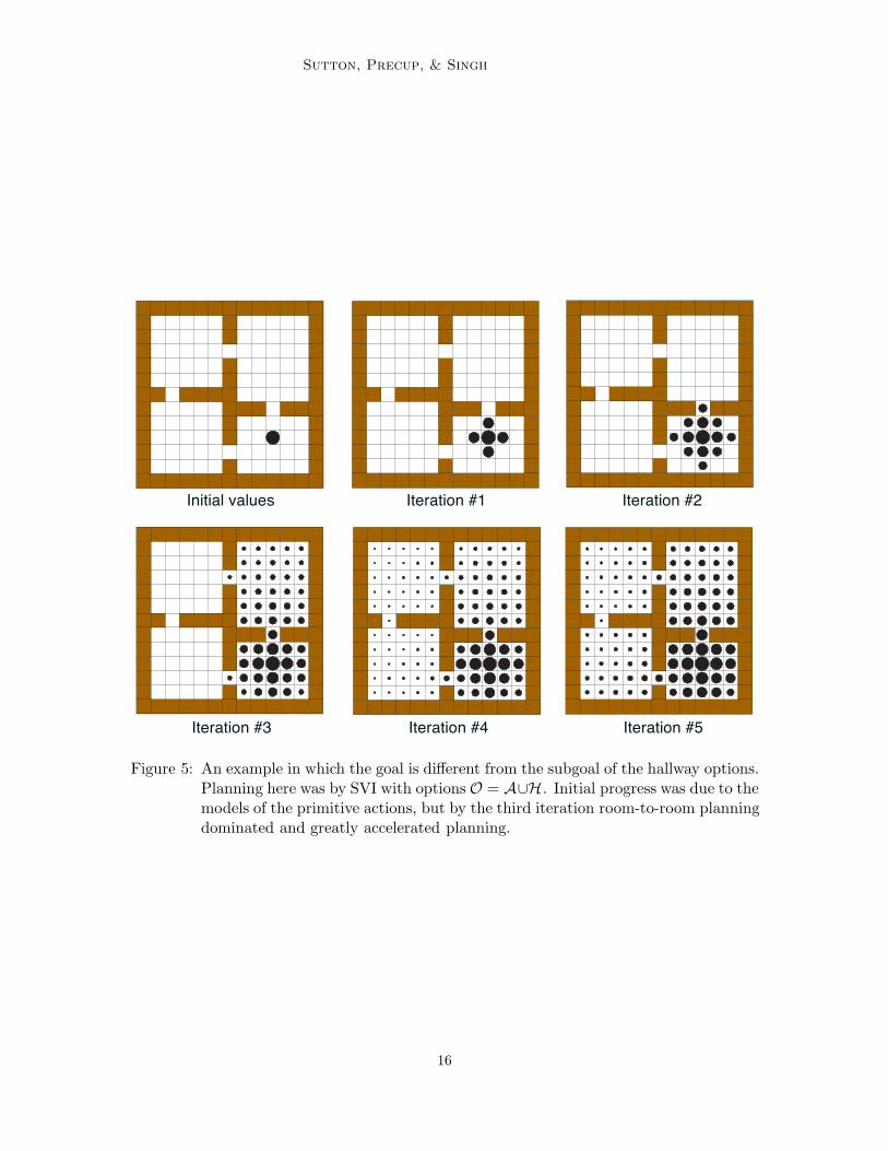
The example above is a particularly favorable case for the use of multi-step optionsbecause the goal state is a hallway, the target state of some of the options. Next weconsider a case in which there is no such coincidence, in which the goal lies in the middleof a room, in the state labeled G2 in Figure 2. The hallway options and their models werejust as in the previous experiment. In this case, planning with (models of) the hallwayoptions alone could never completely solve the task, because these take the agent onlyto hallways and thus never to the goal state. Figure 5 shows the value functions foundover five iterations of SVI using both the hallway options and options corresponding to theprimitive actions (i.e., using O = A -H ). In the first two iterations, accurate values were
4. The o!-target hallway states are exceptions in that they have three possible outcomes: the target hallway,themselves, and the neighboring state in the o!-target room.
15
Sutton, Precup, & Singh
Iteration #1Initial values Iteration #2
Iteration #3 Iteration #4 Iteration #5
Figure 5: An example in which the goal is di!erent from the subgoal of the hallway options.Planning here was by SVI with options O = A-H. Initial progress was due to themodels of the primitive actions, but by the third iteration room-to-room planningdominated and greatly accelerated planning.
16
Between MDPs and Semi-MDPs
propagated from G2 by one cell per iteration by the models corresponding to the primitiveactions. After two iterations, however, the first hallway state was reached, and subsequentlyroom-to-room planning using the temporally extended hallway options dominated. Notehow the lower-left most state was given a nonzero value during iteration three. This valuecorresponds to the plan of first going to the hallway state above and then down to the goal;it was overwritten by a larger value corresponding to a more direct route to the goal in thenext iteration. Because of the options, a close approximation to the correct value functionwas found everywhere by the fourth iteration; without them only the states within threesteps of the goal would have been given non-zero values by this time.
We have used SVI in this example because it is a particularly simple planning methodwhich makes the potential advantage of multi-step options particularly clear. In largeproblems, SVI is impractical because the number of states is too large to complete manyiterations, often not even one. In practice it is often necessary to be very selective about thestates updated, the options considered, and even the next states considered. These issuesare not resolved by multi-step options, but neither are they greatly aggravated. Optionsprovide a tool for dealing with them more flexibly. Planning with options need be nomore complex than planning with actions. In the SVI experiments above there were fourprimitive options and eight hallway options, but in each state only two hallway optionsneeded to be considered. In addition, the models of the primitive actions generate fourpossible successors with non-zero probability whereas the multi-step options generate onlytwo. Thus planning with the multi-step options was actually computationally cheaper thanconventional SVI in this case. In the second experiment this was not the case, but still theuse of multi-step options did not greatly increase the computational costs.
5.2 SMDP Value Learning
The problem of finding an optimal policy over a set of options O can also be addressedby learning methods. Because the MDP augmented by the options is an SMDP, we canapply SMDP learning methods as developed by Bradtke and Du! (1995), Parr and Russell(1998; Parr, in prep.), Mahadevan et al. (1997), or McGovern, Sutton and Fagg (1997).Much as in the planning methods discussed above, each option is viewed as an indivisible,opaque unit. When the execution of option o is started in state s, we next jump to the states" in which o terminates. Based on this experience, an approximate option-value functionQ(s, o) is updated. For example, the SMDP version of one-step Q-learning (Bradtke andDu!, 1995), which we call SMDP Q-learning, updates after each option termination by
Q(s, o) , Q(s, o) + '.r + "k max
a!OQ(s", a) . Q(s, o)
/,
where k denotes the number of time steps elapsing between s and s", r denotes the cumula-tive discounted reward over this time, and it is implicit that the step-size parameter ' maydepend arbitrarily on the states, option, and time steps. The estimate Q(s, o) convergesto Q#
O(s, o) for all s ! S and o ! O under conditions similar to those for conventional Q-learning (Parr, in prep.), from which it is easy to determine an optimal policy as describedearlier.
17
Sutton, Precup, & Singh
Episodes Episodes
Stepsper
episode
A
A
A
H
A U H
A U H
Goalat G!
Goalat G"
1 10 100 1000 10,00010
100
1000
1 10 100 1000 10,00010
100
1000
HH
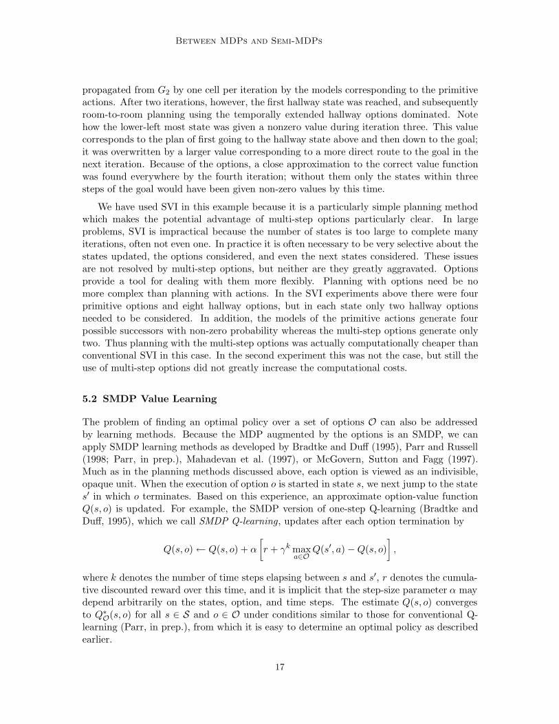
Figure 6: Learning curves for SMDP Q-learning in the rooms example with various goalsand sets of options. After 100 episodes, the data points are averages over bins of10 episodes to make the trends clearer. The step size parameter was optimizedto the nearest power of 2 for each goal and set of options. The results shownused ' = 1
8 in all cases except that with O = H and G1 (' = 116) and that with
O = A -H and G2 (' = 14).
As an illustration, we applied SMDP Q-learning to the rooms example (Figure 2) withthe goal at G1 and at G2. As in the case of planning, we used three di!erent sets of options,A, H, and A -H . In all cases, options were selected from the set according to an (-greedymethod. That is, given the current estimates Q(s, o), let o# = arg maxo!Os Q(s, o) denotethe best valued action (with ties broken randomly). Then the policy used to select optionswas
µ(s, o) =0
1 . ( + (|Os| if o = o#
(|Os| otherwise,
for all s ! S and o ! O, where O is one of A, H, or A-H. The probability of random action,(, was set at 0.1 in all cases. The initial state of each trial was in the upper-left corner.Figure 6 shows learning curves for both goals and all sets of options. In all cases, multi-step options caused the goal to be reached much more quickly, even on the very first trial.With the goal at G1, these methods maintained an advantage over conventional Q-learningthroughout the experiment, presumably because they did less exploration. The results weresimilar with the goal at G2, except that the H method performed worse than the others inthe long term. This is because the best solution requires several steps of primitive actions(the hallway options alone find the best solution running between hallways that sometimesstumbles upon G2). For the same reason, the advantages of the A -H method over the Amethod were also reduced.
18
Between MDPs and Semi-MDPs
6. Termination Improvement
SMDP methods apply to options, but only when they are treated as opaque indivisibleunits. More interesting and potentially more powerful methods are possible by lookinginside options and by altering their internal structure. In this section we take a first step inaltering options to make them more useful. This is the area where working simultaneouslyin terms of MDPs and SMDPs is most relevant. We can analyze options in terms of theSMDP and then use their MDP interpretation to change them and produce a new SMDP.
In particular, in this section we consider altering the termination conditions of options.Note that treating options as indivisible units, as SMDP methods do, is limiting in anunnecessary way. Once an option has been selected, such methods require that its policy befollowed until the option terminates. Suppose we have determined the option-value functionQµ(s, o) for some policy µ and for all state–options pairs s, o that could be encountered whilefollowing µ. This function tells us how well we do while following µ, committing irrevocablyto each option, but it can also be used to re-evaluate our commitment on each step. Supposeat time t we are in the midst of executing option o. If o is Markov in s, then we can comparethe value of continuing with o, which is Qµ(st, o), to the value of terminating o and selectinga new option according to µ, which is V µ(s) =
1q µ(s, q)Qµ(s, q). If the latter is more highly
valued, then why not terminate o and allow the switch? We prove below that this new wayof behaving will indeed be better.
In the following theorem we characterize the new way of behaving as following a policyµ" that is the same as the original policy, µ, but over a new set of options: µ"(s, o") = µ(s, o),for all s ! S. Each new option o" is the same as the corresponding old option o except thatit terminates whenever termination seems better than continuing according to Qµ. In otherwords, the termination condition #" of o" is the same as that of o except that #"(s) = 1 ifQµ(s, o) < V µ(s). We call such a µ" a termination improved policy of µ. The theorem belowgeneralizes on the case described above in that termination improvement is optional, notrequired, at each state where it could be done; this weakens the requirement that Qµ(s, o)be completely known. A more important generalization is that the theorem applies tosemi-Markov options rather than just Markov options. This is an important generalization,but can make the result seem less intuitively accessible on first reading. Fortunately, theresult can be read as restricted to the Markov case simply by replacing every occurrence of“history” with “state”, set of histories, #, with set of states, S, etc.
Theorem 2 (Termination Improvement) For any MDP, any set of options O, andany Markov policy µ : S # O $% [0, 1], define a new set of options, O", with a one-to-onemapping between the two option sets as follows: for every o = 'I,!,#( ! O we define acorresponding o" = 'I,!,#"( ! O", where #" = # except that for any history h that ends instate s and in which Qµ(h, o) < V µ(s), we may choose to set #"(h) = 1. Any histories whosetermination conditions are changed in this way are called termination-improved histories.Let policy µ" be such that for all s ! S, and for all o" ! O", µ"(s, o") = µ(s, o), where o isthe option in O corresponding to o". Then
1. V µ!(s) / V µ(s) for all s ! S.
19
Sutton, Precup, & Singh
2. If from state s ! S there is a non-zero probability of encountering a termination-improved history upon initiating µ" in s, then V µ!(s) > V µ(s).
Proof: Shortly we show that, for an arbitrary start state s, executing the option given bythe termination improved policy µ" and then following policy µ thereafter is no worse thanalways following policy µ. In other words, we show that the following inequality holds:
'
o!µ"(s, o")[ro!
s +'
s!po!
ss!Vµ(s")] / V µ(s) =
'
o
µ(s, o)[ros +
'
s!po
ss!Vµ(s")]. (13)
If this is true, then we can use it to expand the left-hand side, repeatedly replacing everyoccurrence of V µ(x) on the left by the corresponding
1o! µ
"(x, o")[ro!x +
1x! po!
xx!V µ(x")]. Inthe limit, the left-hand side becomes V µ! , proving that V µ! / V µ.
To prove the inequality in (13), we note that for all s, µ"(s, o") = µ(s, o), and show that
ro!s +
'
s!po!
ss!Vµ(s") / ro
s +'
s!po
ss!Vµ(s") (14)
as follows. Let % denote the set of all termination improved histories: % = {h ! # : #(h) "=#"(h)}. Then,
ro!s +
'
s!po!
ss!Vµ(s") = E
$r + "kV µ(s")
%%% E(o", s), hss! "! %&+E
$r + "kV µ(s")
%%% E(o", s), hss! ! %&,
where s", r, and k are the next state, cumulative reward, and number of elapsed stepsfollowing option o from s (hss! is the history from s to s"). Trajectories that end because ofencountering a history not in % never encounter a history in %, and therefore also occur withthe same probability and expected reward upon executing option o in state s. Therefore, ifwe continue the trajectories that end because of encountering a history in % with option ountil termination and thereafter follow policy µ, we get
E$r + "kV µ(s")
%%% E(o", s), hss! "! %&
+ E$#(s")[r + "kV µ(s")] + (1 . #(s"))[r + "kQµ(hss! , o)]
%%% E(o", s), hss! ! %&
= ros +
'
s!po
ss!Vµ(s"),
because option o is semi-Markov. This proves (13) because for all hss! ! %, QµO(hss! , o) )
V µ(s"). Note that strict inequality holds in (14) if QµO(hss! , o) < V µ(s") for at least one
history hss! ! % that ends a trajectory generated by o" with non-zero probability. +
As one application of this result, consider the case in which µ is an optimal policy forsome given set of Markov options O. We have already discussed how we can, by planningor learning, determine the optimal value functions V #
O and Q#O and from them the optimal
policy µ#O that achieves them. This is indeed the best that can be done without changingO,
that is, in the SMDP defined by O, but less than the best possible achievable in the MDP,which is V # = V #
A. But of course we typically do not wish to work directly in the primitiveoptions A because of the computational expense. The termination improvement theorem
20
Between MDPs and Semi-MDPs
gives us a way of improving over µ#O with little additional computation by stepping outside
O. That is, at each step we interrupt the current option and switch to any new option thatis valued more highly according to Q#
O. Checking for such options can typically be done atvastly less expense per time step than is involved in the combinatorial process of computingQ#
O. In this sense, termination improvement gives us a nearly free improvement over anySMDP planning or learning method that computes Q#
O as an intermediate step. Kaelbling(1993) was the first to demonstrate this e!ect—improved performance by interrupting atemporally extended substep based on a value function found by planning at a higherlevel—albeit in a more restricted setting than we consider here.
In the extreme case, we might interrupt on every step and switch to the greedy option—the option in that state that is most highly valued according to Q#
O. In this case, optionsare never followed for more than one step, and they might seem superfluous. However,the options still play a role in determining Q#
O, the basis on which the greedy switches aremade, and recall that multi-step options enable Q#
O to be found much more quickly than Q#
could (Section 5). Thus, even if multi-step options are never actually followed for more thanone step, they still provide substantial advantages in computation and in our theoreticalunderstanding.
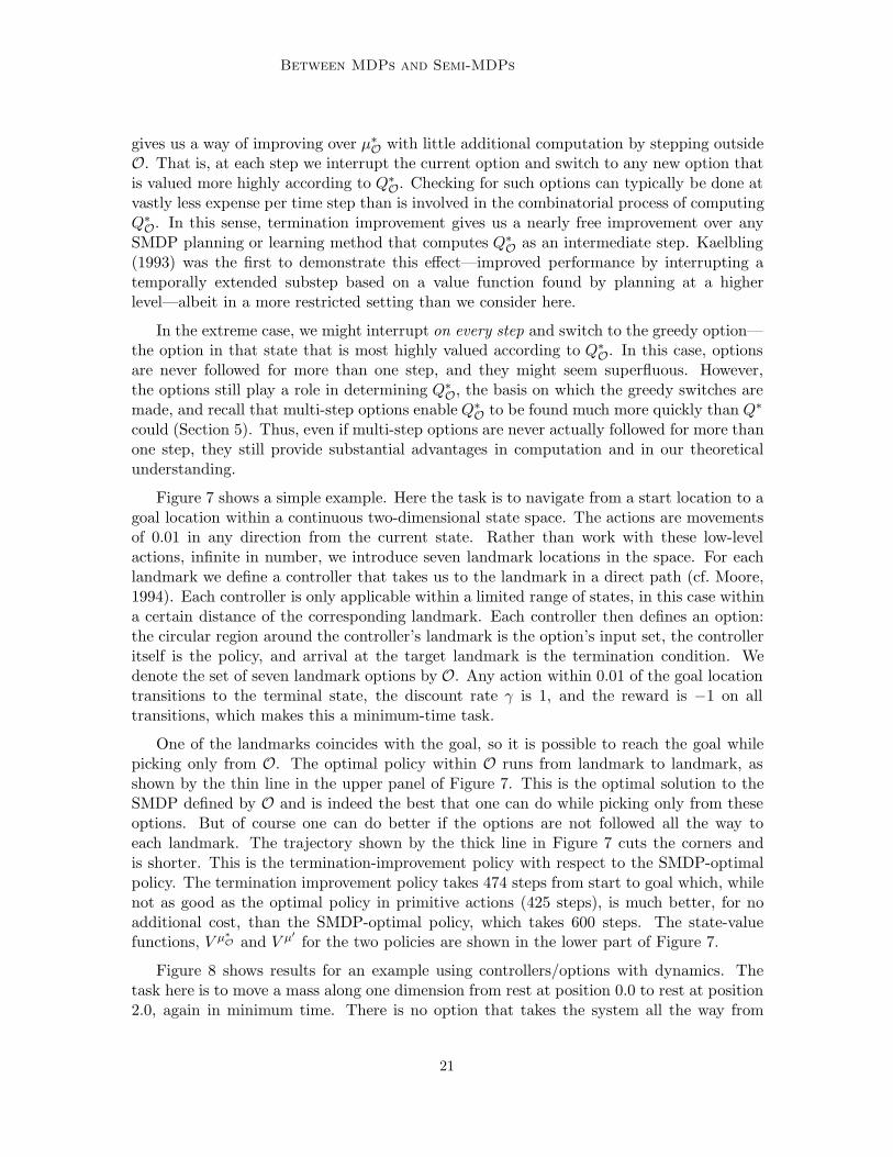
Figure 7 shows a simple example. Here the task is to navigate from a start location to agoal location within a continuous two-dimensional state space. The actions are movementsof 0.01 in any direction from the current state. Rather than work with these low-levelactions, infinite in number, we introduce seven landmark locations in the space. For eachlandmark we define a controller that takes us to the landmark in a direct path (cf. Moore,1994). Each controller is only applicable within a limited range of states, in this case withina certain distance of the corresponding landmark. Each controller then defines an option:the circular region around the controller’s landmark is the option’s input set, the controlleritself is the policy, and arrival at the target landmark is the termination condition. Wedenote the set of seven landmark options by O. Any action within 0.01 of the goal locationtransitions to the terminal state, the discount rate " is 1, and the reward is .1 on alltransitions, which makes this a minimum-time task.
One of the landmarks coincides with the goal, so it is possible to reach the goal whilepicking only from O. The optimal policy within O runs from landmark to landmark, asshown by the thin line in the upper panel of Figure 7. This is the optimal solution to theSMDP defined by O and is indeed the best that one can do while picking only from theseoptions. But of course one can do better if the options are not followed all the way toeach landmark. The trajectory shown by the thick line in Figure 7 cuts the corners andis shorter. This is the termination-improvement policy with respect to the SMDP-optimalpolicy. The termination improvement policy takes 474 steps from start to goal which, whilenot as good as the optimal policy in primitive actions (425 steps), is much better, for noadditional cost, than the SMDP-optimal policy, which takes 600 steps. The state-valuefunctions, V µ"
O and V µ! for the two policies are shown in the lower part of Figure 7.
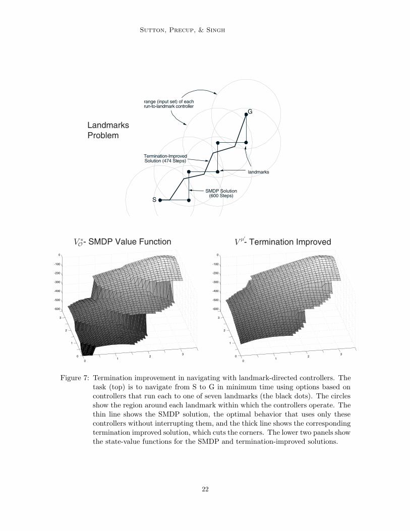
Figure 8 shows results for an example using controllers/options with dynamics. Thetask here is to move a mass along one dimension from rest at position 0.0 to rest at position2.0, again in minimum time. There is no option that takes the system all the way from
21
Sutton, Precup, & Singh
SMDP Solution(600 Steps)
Termination-ImprovedSolution (474 Steps)
range (input set) of eachrun-to-landmark controller
landmarks
S
G
01
23
0
1
2
3
-600
-500
-400
-300
-200
-100
0
01
23
0
1
2
3
-600
-500
-400
-300
-200
-100
0
V - SMDP Value Function*Oµ#
LandmarksProblem
V - Termination Improved
Figure 7: Termination improvement in navigating with landmark-directed controllers. Thetask (top) is to navigate from S to G in minimum time using options based oncontrollers that run each to one of seven landmarks (the black dots). The circlesshow the region around each landmark within which the controllers operate. Thethin line shows the SMDP solution, the optimal behavior that uses only thesecontrollers without interrupting them, and the thick line shows the correspondingtermination improved solution, which cuts the corners. The lower two panels showthe state-value functions for the SMDP and termination-improved solutions.
22
Between MDPs and Semi-MDPs
0
0.02
0.04
0.06
0 0.5 1 1.5 2
Position
Velocity
TerminationImproved
121 Steps
SMDP Solution210 Steps
Figure 8: Phase-space plot of the SMDP and termination improved policies in a simpledynamical task. The system is a mass moving in one dimension: xt+1 = xt+ xt+1,xt+1 = xt+at.0.175xt where xt is the position, xt the velocity, 0.175 a coe"cientof friction, and the action at an applied force. Two controllers are provided asoptions, one that drives the position to zero velocity at x# = 1.0 and the otherto x# = 2.0. Whichever option is being followed at time t, its target position x#
determines the action taken, according to at = 0.01(x# . xt).
23
Sutton, Precup, & Singh
0.0 to 2.0, but we do have an option that takes it from 0.0 to 1.0 and another option thattakes it from any position greater than 0.5 to 2.0. Both options control the system preciselyto its target position and to zero velocity, terminating only when both of these are correctto within ( = 0.0001. Using just these options, the best that can be done is to first moveprecisely to rest at 1.0, using the first option, then re-accelerate and move to 2.0 usingthe second option. This SMDP-optimal solution is much slower than the correspondingtermination improved policy, as shown in Figure 8. Because of the need to slow down tonear-zero velocity at 1.0, it takes over 200 time steps, whereas the improved policy takesonly 121 steps.
7. Intra-Option Model Learning
The models of an option, ros and po
ss!, can be learned from experience given knowledge ofthe option (i.e., of its I, !, and #). For a semi-Markov option, the only general approachis to execute the option to termination many times in each state s, recording in each casethe resultant next state s", cumulative discounted reward r, and elapsed time k. Theseoutcomes are then averaged to approximate the expected values for ro
s and poss! given by (5)
and (6). For example, an incremental learning rule for this could update its estimates ros
and posx, for all x ! S, after each execution of o in state s, by
ros = ro
s + '[r . ros ], (15)
andpo
sx = posx + '["k$xs! . po
sx], (16)
where the step-size parameter, ', may be constant or may depend on the state, option, andtime. For example, if ' is 1 divided by the number of times that o has been experienced in s,then these updates maintain the estimates as sample averages of the experienced outcomes.However the averaging is done, we call these SMDP model-learning methods because, likeSMDP value-learning methods, they are based on jumping from initiation to terminationof each option, ignoring what happens along the way. In the special case in which o is aprimitive action, SMDP model-learning methods reduce to those used to learn conventionalone-step models of actions.
One drawback to SMDP model-learning methods is that they improve the model ofan option only when the option terminates. Because of this, they cannot be used fornonterminating options and can only be applied to one option at a time—the one optionthat is executing at that time. For Markov options, special temporal-di!erence methodscan be used to learn usefully about the model of an option before the option terminates.We call these intra-option methods because they learn from experience within a singleoption. Intra-option methods can even be used to learn about the model of an optionwithout ever executing the option, as long as some selections are made that are consistentwith the option. Intra-option methods are examples of o!-policy learning methods (Suttonand Barto, 1998) because they learn about the consequences of one policy while actuallybehaving according to another, potentially di!erent policy. Intra-option methods can beused to simultaneously learn models of many di!erent options from the same experience.
24
Between MDPs and Semi-MDPs
Intra-option methods were introduced by Sutton (1995), but only for a prediction problemwith a single unchanging policy, not the full control case we consider here.
Just as there are Bellman equations for value functions, there are also Bellman equationsfor models of options. Consider the intra-option learning of the model of a Markov optiono = 'I,!,#(. The correct model of o is related to itself by
ros =
'
a!As
!(s, a)E$r + "(1 . #(s"))ro
s!
&
where r and s" are the reward and next state given that action a is taken in state s,
='
a!As
!(s, a)(
ras +
'
s!pa
ss!(1 . #(s"))ros!
)
,
and
posx =
'
a!As
!(s, a)"E$(1 . #(s"))po
s!x + #(s")$s!x
&
='
a!As
!(s, a)'
s!pa
ss!(1 . #(s"))pos!x + #(s")$s!x
for all s, x ! S. How can we turn these Bellman-like equations into update rules for learningthe model? First consider that action at is taken in st, and that the way it was selectedis consistent with o = 'I,!,#(, that is, that at was selected with the distribution !(st, ·).Then the Bellman equations above suggest the temporal-di!erence update rules
rost, ro
st+ '
2rt+1 + "(1 . #(st+1))ro
st+1. ro
st
3(17)
andpo
stx , postx + '
2"(1 . #(st+1))po
st+1x + "#(st+1)$st+1x . postx
3, (18)
where poss! and ro
s are the estimates of poss! and ro
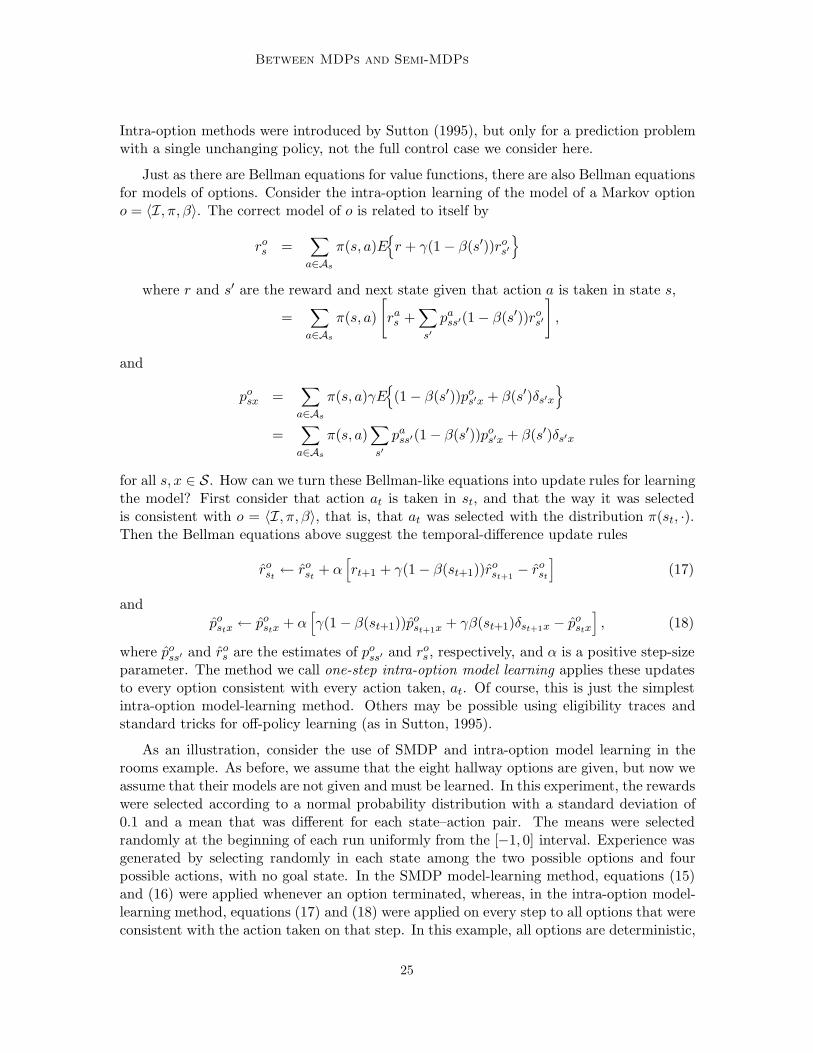
s , respectively, and ' is a positive step-sizeparameter. The method we call one-step intra-option model learning applies these updatesto every option consistent with every action taken, at. Of course, this is just the simplestintra-option model-learning method. Others may be possible using eligibility traces andstandard tricks for o!-policy learning (as in Sutton, 1995).
As an illustration, consider the use of SMDP and intra-option model learning in therooms example. As before, we assume that the eight hallway options are given, but now weassume that their models are not given and must be learned. In this experiment, the rewardswere selected according to a normal probability distribution with a standard deviation of0.1 and a mean that was di!erent for each state–action pair. The means were selectedrandomly at the beginning of each run uniformly from the [.1, 0] interval. Experience wasgenerated by selecting randomly in each state among the two possible options and fourpossible actions, with no goal state. In the SMDP model-learning method, equations (15)and (16) were applied whenever an option terminated, whereas, in the intra-option model-learning method, equations (17) and (18) were applied on every step to all options that wereconsistent with the action taken on that step. In this example, all options are deterministic,
25
Sutton, Precup, & Singh
0
1
2
3
4
0 20,000 40,000 60,000 80,000 100,000
Options Executed Options Executed
SMDP
IntraSMDP 1/t
SMDP
Intra
SMDP 1/t
Reward Prediction
ErrorState
Prediction Error
Max Error
Avg. Error
0
0.1
0.2
0.3
0.4
0.5
0.6
0.7
0 20,000 40,000 60,000 80,000 100,000
SMDP
SMDP
SMDP 1/t
Intra
Intra
SMDP 1/t
Max ErrorAvg. Error
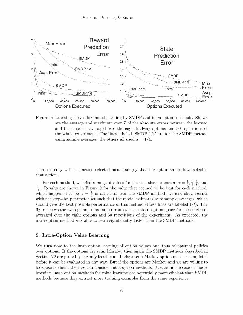
Figure 9: Learning curves for model learning by SMDP and intra-option methods. Shownare the average and maximum over I of the absolute errors between the learnedand true models, averaged over the eight hallway options and 30 repetitions ofthe whole experiment. The lines labeled ‘SMDP 1/t’ are for the SMDP methodusing sample averages; the others all used ' = 1/4.
so consistency with the action selected means simply that the option would have selectedthat action.
For each method, we tried a range of values for the step-size parameter, ' = 12 , 1
4 , 18 , and
116 . Results are shown in Figure 9 for the value that seemed to be best for each method,which happened to be ' = 1
4 in all cases. For the SMDP method, we also show resultswith the step-size parameter set such that the model estimates were sample averages, whichshould give the best possible performance of this method (these lines are labeled 1/t). Thefigure shows the average and maximum errors over the state–option space for each method,averaged over the eight options and 30 repetitions of the experiment. As expected, theintra-option method was able to learn significantly faster than the SMDP methods.
8. Intra-Option Value Learning
We turn now to the intra-option learning of option values and thus of optimal policiesover options. If the options are semi-Markov, then again the SMDP methods described inSection 5.2 are probably the only feasible methods; a semi-Markov option must be completedbefore it can be evaluated in any way. But if the options are Markov and we are willing tolook inside them, then we can consider intra-option methods. Just as in the case of modellearning, intra-option methods for value learning are potentially more e"cient than SMDPmethods because they extract more training examples from the same experience.
26
Between MDPs and Semi-MDPs
For example, suppose we are learning to approximate Q#O(s, o) and that o is Markov.
Based on an execution of o from t to t+k, SMDP methods extract a single training examplefor Q#
O(s, o). But because o is Markov, it is, in a sense, also initiated at each of the stepsbetween t and t+k. The jumps from each intermediate si to st+k are also valid experienceswith o, experiences that can be used to improve estimates of Q#
O(si, o). Or consider anoption that is very similar to o and which would have selected the same actions, but whichwould have terminated one step later, at t + k + 1 rather than at t + k. Formally this is adi!erent option, and formally it was not executed, yet all this experience could be used forlearning relevant to it. In fact, an option can often learn something from experience that isonly slightly related (occasionally selecting the same actions) to what would be generatedby executing the option. This is the idea of o!-policy training—to make full use of whateverexperience occurs to learn as much as possible about all options irrespective of their role ingenerating the experience. To make the best use of experience we would like an o!-policyand intra-option version of Q-learning.
It is convenient to introduce new notation for the value of a state–option pair given thatthe option is Markov and executing upon arrival in the state:
U#O(s, o) = (1 . #(s))Q#
O(s, o) + #(s)maxo!!O
Q#O(s, o"),
Then we can write Bellman-like equations that relate Q#O(s, o) to expected values of U#
O(s", o),where s" is the immediate successor to s after initiating Markov option o = 'I,!,#( in s:
Q#O(s, o) =
'
a!As
!(s, a)E$r + "U#
O(s", o)%%% s, a
&
='
a!As
!(s, a)(
ras +
'
s!pa
ss!U#O(s", o)
)
, (19)
where r is the immediate reward upon arrival in s". Now consider learning methods basedon this Bellman equation. Suppose action at is taken in state st to produce next state st+1
and reward rt+1, and that at was selected in a way consistent with the Markov policy !of an option o = 'I,!,#(. That is, suppose that at was selected according to the distri-bution !(st, ·). Then the Bellman equation above suggests applying the o!-policy one-steptemporal-di!erence update:
Q(st, o) , Q(st, o) + '2(rt+1 + "U(st+1, o)) . Q(st, o)
3, (20)
whereU(s, o) = (1 . #(s))Q(s, o) + #(s)max
o!!OQ(s, o").
The method we call one-step intra-option Q-learning applies this update rule to every optiono consistent with every action taken, at. Note that the algorithm is potentially dependenton the order in which options are updated.
Theorem 3 (Convergence of intra-option Q-learning) For any set of deterministicMarkov options O, one-step intra-option Q-learning converges w.p.1 to the optimal Q-values, Q#
O, for every option regardless of what options are executed during learning providedevery primitive action gets executed in every state infinitely often.
27
Sutton, Precup, & Singh
Proof: (Sketch) On experiencing the transition, (s, a, r", s"), for every option o that picksaction a in state s, intra-option Q-learning performs the following update:
Q(s, o) , Q(s, o) + '(s, o)[r" + "U(s", o) . Q(s, o)].
Let a be the action selection by deterministic Markov option o = 'I,!,#(. Our resultfollows directly from Theorem 1 of Jaakkola, Jordan, and Singh (1994) and the observationthat the expected value of the update operator r" + "U(s", o) yields a contraction, provedbelow:
|E{r" + "U(s", o)}. Q#O(s, o)| = |ra
s +'
s!pa
ss!U(s", o) . Q#O(s, o)|
= |ras +
'
s!pa
ss!U(s", o) . ras .
'
s!pa
ss!U#O(s", o)|
) |'
s!pa
ss!
2(1 . #(s"))(Q(s", o) . Q#
O(s", o))
+#(s")(maxo!!O
Q(s", o") . maxo!!O
Q#O(s", o")
3|
)'
s!pa
ss! maxs!!,o!!
|Q(s"", o"") . Q#O(s"", o"")|
) " maxs!!,o!!
|Q(s"", o"") . Q#O(s"", o"")|
+
As an illustration, we applied this intra-option method to the rooms example, this timewith the goal in the rightmost hallway, cell G1 in Figure 2. Actions were selected randomlywith equal probability from the four primitives. The update (20) was applied first to theprimitive options, then to any of the hallway options that were consistent with the action.The hallway options were updated in clockwise order, starting from any hallways that facedup from the current state. The rewards were the same as in the experiment in the previoussection. Figure 10 shows learning curves demonstrating the e!ective learning of optionvalues without ever selecting the corresponding options.
Intra-option versions of other reinforcement learning methods such as Sarsa, TD()), andeligibility-trace versions of Sarsa and Q-learning should be straightforward, although therehas been no experience with them. The intra-option Bellman equation (19) could also beused for intra-option sample-based planning.
9. Learning Options
Perhaps the most important aspect of working between MDPs and SMDPs is that theoptions making up the SMDP actions may be changed. We have seen one way in whichthis can be done by changing their termination conditions. Perhaps more fundamental thanthat is changing their policies, which we consider briefly in this section. It is natural tothink of options as achieving subgoals of some kind, and to adapt each option’s policy tobetter achieve its subgoal. For example, if the option is open-the-door, then it is natural
28
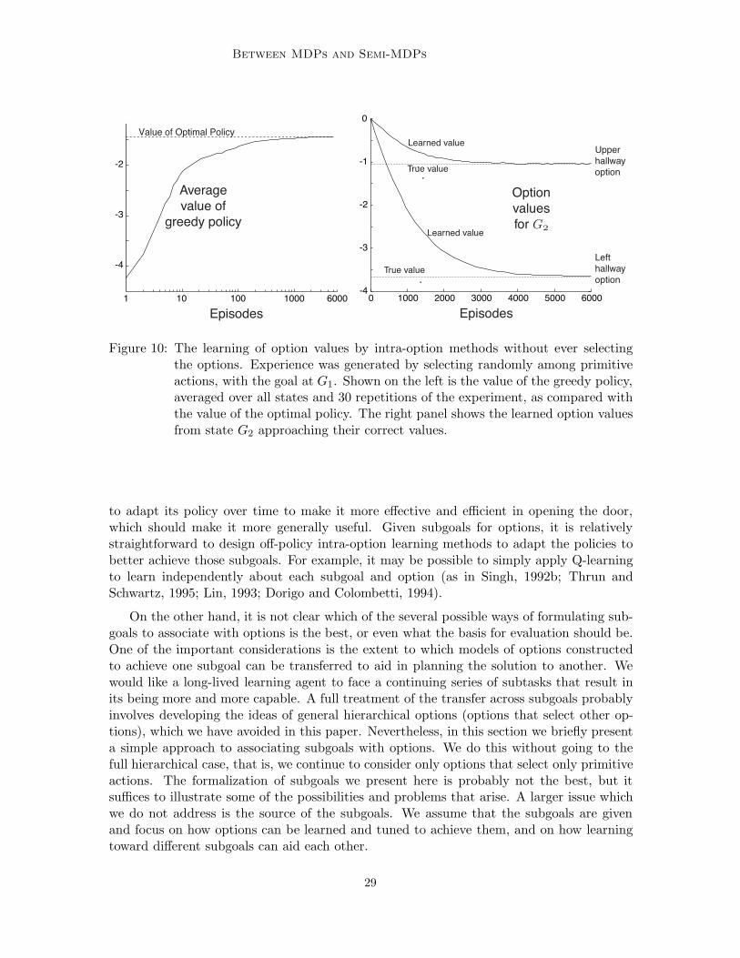
Between MDPs and Semi-MDPs
-4
-3
-2
-1
0
0 10001000 6000 2000 3000 4000 5000 6000
EpisodesEpisodes
Option
values
for G%
Average
value of
greedy policy
Learned value
Learned value
Upper
hallway
option
Left
hallway
option
True value
True value-4
-3
-2
1 10 100
Value of Optimal Policy
Figure 10: The learning of option values by intra-option methods without ever selectingthe options. Experience was generated by selecting randomly among primitiveactions, with the goal at G1. Shown on the left is the value of the greedy policy,averaged over all states and 30 repetitions of the experiment, as compared withthe value of the optimal policy. The right panel shows the learned option valuesfrom state G2 approaching their correct values.
to adapt its policy over time to make it more e!ective and e"cient in opening the door,which should make it more generally useful. Given subgoals for options, it is relativelystraightforward to design o!-policy intra-option learning methods to adapt the policies tobetter achieve those subgoals. For example, it may be possible to simply apply Q-learningto learn independently about each subgoal and option (as in Singh, 1992b; Thrun andSchwartz, 1995; Lin, 1993; Dorigo and Colombetti, 1994).
On the other hand, it is not clear which of the several possible ways of formulating sub-goals to associate with options is the best, or even what the basis for evaluation should be.One of the important considerations is the extent to which models of options constructedto achieve one subgoal can be transferred to aid in planning the solution to another. Wewould like a long-lived learning agent to face a continuing series of subtasks that result inits being more and more capable. A full treatment of the transfer across subgoals probablyinvolves developing the ideas of general hierarchical options (options that select other op-tions), which we have avoided in this paper. Nevertheless, in this section we briefly presenta simple approach to associating subgoals with options. We do this without going to thefull hierarchical case, that is, we continue to consider only options that select only primitiveactions. The formalization of subgoals we present here is probably not the best, but itsu"ces to illustrate some of the possibilities and problems that arise. A larger issue whichwe do not address is the source of the subgoals. We assume that the subgoals are givenand focus on how options can be learned and tuned to achieve them, and on how learningtoward di!erent subgoals can aid each other.
29
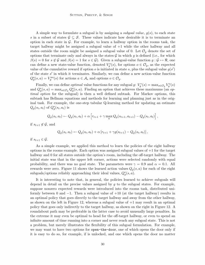
Sutton, Precup, & Singh
A simple way to formulate a subgoal is by assigning a subgoal value, g(s), to each states in a subset of states G & S. These values indicate how desirable it is to terminate anoption in each state in G. For example, to learn a hallway option in the rooms task, thetarget hallway might be assigned a subgoal value of +1 while the other hallway and allstates outside the room might be assigned a subgoal value of 0. Let Og denote the set ofoptions that terminate only and always in the states G in which g is defined (i.e., for which#(s) = 0 for s "! G and #(s) = 1 for s ! G). Given a subgoal-value function g : G $% 0, onecan define a new state-value function, denoted V o
g (s), for options o ! Og, as the expectedvalue of the cumulative reward if option o is initiated in state s, plus the subgoal value g(s")of the state s" in which it terminates. Similarly, we can define a new action-value functionQo
g(s, a) = V aog (s) for actions a ! As and options o ! Og.
Finally, we can define optimal value functions for any subgoal g: V #g (s) = maxo!Og V o
g (s)and Q#
g(s, a) = maxo!Og Qog(s, a). Finding an option that achieves these maximums (an op-
timal option for the subgoal) is then a well defined subtask. For Markov options, thissubtask has Bellman equations and methods for learning and planning just as in the orig-inal task. For example, the one-step tabular Q-learning method for updating an estimateQg(st, at) of Q#
g(st, at) is
Qg(st, at) , Qg(st, at) + '2rt+1 + " max
aQg(st+1, at+1) . Qg(st, at)
3,
if st+1 "! G, and
Qg(st, at) , Qg(st, at) + ' [rt+1 + "g(st+1) . Qg(st, at)] ,
if st+1 ! G.
As a simple example, we applied this method to learn the policies of the eight hallwayoptions in the rooms example. Each option was assigned subgoal values of +1 for the targethallway and 0 for all states outside the option’s room, including the o!-target hallway. Theinitial state was that in the upper left corner, actions were selected randomly with equalprobability, and there was no goal state. The parameters were " = 0.9 and ' = 0.1. Allrewards were zero. Figure 11 shows the learned action values Qg(s, a) for each of the eightsubgoals/options reliably approaching their ideal values, Q#
g(s, a).
It is interesting to note that, in general, the policies learned to achieve subgoals willdepend in detail on the precise values assigned by g to the subgoal states. For example,suppose nonzero expected rewards were introduced into the rooms task, distributed uni-formly between 0 and .1. Then a subgoal value of +10 (at the target hallway) results inan optimal policy that goes directly to the target hallway and away from the other hallway,as shown on the left in Figure 12, whereas a subgoal value of +1 may result in an optimalpolicy that goes only indirectly to the target hallway, as shown on the right in Figure 12. Aroundabout path may be preferable in the latter case to avoid unusually large penalties. Inthe extreme it may even be optimal to head for the o!-target hallway, or even to spend aninfinite amount of time running into a corner and never reach any subgoal state. This is nota problem, but merely illustrates the flexibility of this subgoal formulation. For example,we may want to have two options for open-the-door, one of which opens the door only ifit is easy to do so, for example, if is unlocked, and one which opens the door no matter
30
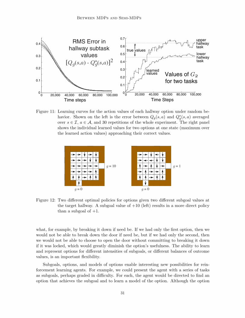
Between MDPs and Semi-MDPs
Time steps
RMS Error inhallway subtask
values
0
0.1
0.2
0.3
0.4
0.5
0.6
0.7
0 20,000 40,000
Time Steps60,000
upperhallwaytask
true values
learnedvalues
lowerhallwaytask
80,000 100,000
Values of G!for two tasks
0
0.1
0.2
0.3
0.4
0 20,000 40,000 60,000 80,000 100,000
[Qg(s,a) - Qg(s,a)]2*
Figure 11: Learning curves for the action values of each hallway option under random be-havior. Shown on the left is the error between Qg(s, a) and Q#
g(s, a) averagedover s ! I, a ! A, and 30 repetitions of the whole experiment. The right panelshows the individual learned values for two options at one state (maximum overthe learned action values) approaching their correct values.
g = 10 g = 1
g = 0 g = 0
Figure 12: Two di!erent optimal policies for options given two di!erent subgoal values atthe target hallway. A subgoal value of +10 (left) results in a more direct policythan a subgoal of +1.
what, for example, by breaking it down if need be. If we had only the first option, then wewould not be able to break down the door if need be, but if we had only the second, thenwe would not be able to choose to open the door without committing to breaking it downif it was locked, which would greatly diminish the option’s usefulness. The ability to learnand represent options for di!erent intensities of subgoals, or di!erent balances of outcomevalues, is an important flexibility.
Subgoals, options, and models of options enable interesting new possibilities for rein-forcement learning agents. For example, we could present the agent with a series of tasksas subgoals, perhaps graded in di"culty. For each, the agent would be directed to find anoption that achieves the subgoal and to learn a model of the option. Although the option
31
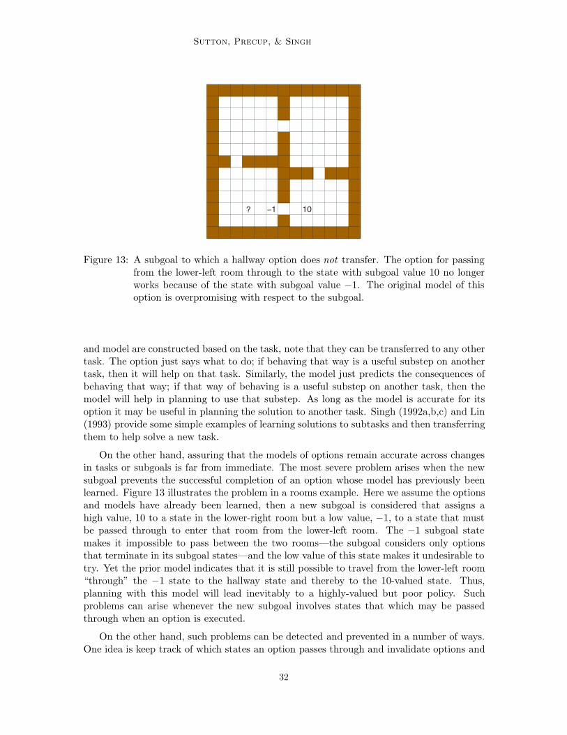
Sutton, Precup, & Singh
10!1?
Figure 13: A subgoal to which a hallway option does not transfer. The option for passingfrom the lower-left room through to the state with subgoal value 10 no longerworks because of the state with subgoal value .1. The original model of thisoption is overpromising with respect to the subgoal.
and model are constructed based on the task, note that they can be transferred to any othertask. The option just says what to do; if behaving that way is a useful substep on anothertask, then it will help on that task. Similarly, the model just predicts the consequences ofbehaving that way; if that way of behaving is a useful substep on another task, then themodel will help in planning to use that substep. As long as the model is accurate for itsoption it may be useful in planning the solution to another task. Singh (1992a,b,c) and Lin(1993) provide some simple examples of learning solutions to subtasks and then transferringthem to help solve a new task.
On the other hand, assuring that the models of options remain accurate across changesin tasks or subgoals is far from immediate. The most severe problem arises when the newsubgoal prevents the successful completion of an option whose model has previously beenlearned. Figure 13 illustrates the problem in a rooms example. Here we assume the optionsand models have already been learned, then a new subgoal is considered that assigns ahigh value, 10 to a state in the lower-right room but a low value, .1, to a state that mustbe passed through to enter that room from the lower-left room. The .1 subgoal statemakes it impossible to pass between the two rooms—the subgoal considers only optionsthat terminate in its subgoal states—and the low value of this state makes it undesirable totry. Yet the prior model indicates that it is still possible to travel from the lower-left room“through” the .1 state to the hallway state and thereby to the 10-valued state. Thus,planning with this model will lead inevitably to a highly-valued but poor policy. Suchproblems can arise whenever the new subgoal involves states that which may be passedthrough when an option is executed.
On the other hand, such problems can be detected and prevented in a number of ways.One idea is keep track of which states an option passes through and invalidate options and
32
Between MDPs and Semi-MDPs
models that pass through subgoal states. Another idea is to alter the subgoal formulationsuch that subgoal states can be passed through: stopping in them and collecting the subgoalvalue is optional rather than required. Finally, note that we do not require models to beaccurate, just non-overpromising—that is, they do not have to predict the correct outcome,just an outcome that is less than or equal to, in expected value, the correct outcome. Thisfinesse may enable important special cases to be handled simply. For example, any newsubgoal involving states G that all have the same subgoal value, e.g., any singleton G, canprobably be safely transferred to. The sort of problem shown in Figure 13 can never occurin such cases.
10. Conclusion
Representing knowledge flexibly at multiple levels of temporal abstraction has the potentialto greatly speed planning and learning on large problems. Options and their models o!era new set of tools for realizing this potential. They o!er new capabilities in each of threecritical areas that we identified at the beginning of this paper. They are clear enough tobe interpreted entirely mechanically, as we have shown by exhibiting simple proceduresfor executing options, learning models of them, testing the models against real events,modifying options, and creating new options given subgoals. They are more expressivethan previous methods based on MDPs and SMDPs in that they permit multiple levelsof temporal abstraction to simultaneously apply to the same system. Finally, they areexplicitly designed to be suitable for planning using methods based on Bellman equations.Compared to conventional MDP and SMDP formulations, options provide a substantialincrease in expressiveness with no loss of clarity or suitability for planning. Compared withclassical AI representations, they are a substantial increase in clarity and in some aspectsof expressiveness. In particular, they apply to stochastic environments, closed-loop policies,and to a more general class of goals.
The foundation for the theory of options is provided by the existing theory of Semi-MDPs. The fact that each set of options defines an SMDP provides a rich set of planningand learning methods, convergence theory, and an immediate, natural, and general way ofanalyzing mixtures of actions at di!erent time scales. This theory o!ers a lot, but stillthe most interesting cases are beyond it because they involve interrupting, constructing, orotherwise decomposing options into their constituent parts. It is the intermediate groundbetween MDPs and SMDPs that seems richest in possibilities for new algorithms and results.In this paper we have broken this ground and touched on many of the issues, but there is farmore left to be done. Key issues such as transfer between subtasks, the source of subgoals,and integration with state abstraction remain open and unclear. The connection betweenoptions and SMDPs provides only a foundation for addressing these and other issues.
Finally, although this paper has emphasized temporally extended action, it is interestingto note that there may be implications for temporally extended perception as well. It is nowcommon to recognize that action and perception are intimately related. To see the objectsin a room is not so much to label or locate them as it is to know what opportunities theya!ord for action: a door to open, a chair to sit on, a book to read, a person to talk to. If the
33
Sutton, Precup, & Singh
temporally extended actions are modeled as options, then perhaps the model of the optioncorresponds well to these perceptions. Consider a robot learning to recognize its batterycharger. The most useful concept for it is the set of states from which it can successfullydock with the charger. This is exactly the concept that would be produced by the model ofa docking option. These kinds of action-oriented concepts are appealing because they canbe tested and learned by the robot without external supervision, as we have shown in thispaper.
Acknowledgements
The authors gratefully acknowledge the substantial help they have received from the col-leagues who have shared their related results and ideas with us over the long period duringwhich this paper was in preparation, especially Amy McGovern, Andy Barto, Ron Parr, TomDietterich, Andrew Fagg, and Manfred Huber. We also thank Leo Zelevinsky, Zsolt Kalmar,Csaba Szepesvari, Andras Lorincz, Paul Cohen, Robbie Moll, Mance Harmon, Sascha En-gelbrecht, and Ted Perkins. This work was supported by NSF grant ECS-9511805 and grantAFOSR-F49620-96-1-0254, both to Andrew Barto and Richard Sutton. Doina Precup alsoacknowledges the support of the Fulbright foundation. Satinder Singh was supported byNSF grant IIS-9711753.
References
Araujo, E.G., Grupen, R.A. (1996). Learning control composition in a complex environ-ment. Proceedings of the Fourth International Conference on Simulation of AdaptiveBehavior, pp. 333-342.
Asada, M., Noda, S., Tawaratsumida, S., Hosada, K. (1996). Purposive behavior acquisitionfor a real robot by vision-based reinforcement learning. Machine Learning 23:279–303.
Barto, A.G., Bradtke, S.J., Singh, S.P. (1995). Learning to act using real-time dynamicprogramming. Artificial Intelligence 72:81–138.
Boutilier, C., Brafman, R.I., Geib, C. (1997). Prioritized goal Decomposition of Markovdecision processes: Toward a synthesis of classical and decision theoretic planning.Proceedings of the Fifteenth International Joint Conference on Artificial Intelligence,pp. 1165–1162.
Bradtke, S.J., and Du!, M.O. (1995). Reinforcement learning methods for continuous-time Markov decision problems. Advances in Neural Information Processing Systems8:393–400. MIT Press, Cambridge, MA.
Brafman, R.I., Moshe, T. (1997). Modeling agents as qualitative decision makers. ArtificialIntelligence 94(1):217-268.
Brockett, R.W. (1993). Hybrid models for motion control systems. In Essays in Control:Perspectives in the Theory and and its Applications, pp. 29–53. Birkhauser, Boston.
34
Between MDPs and Semi-MDPs
Brooks, R. (1986). A robust layered control system for a mobile robot. IEEE journal ofRobotics and Automation, 14–23.
Chrisman, L. (1994). Reasoning about probabilistic actions at multiple levels of granularity,AAAI Spring Symposium: Decision-Theoretic Planning, Stanford University.
Colombetti, M., Dorigo, M., Borghi, G. (1996). Behavior analysis and training: A methodol-ogy for behavior engineering. IEEE Transactions on Systems, Man, and Cybernetics-Part B 26(3):365–380
Crites, R.H., and Barto, A.G. (1996). Improving elevator performance using reinforcementlearning. Advances in Neural Information Processing Systems 9:1017–1023. MITPress, Cambridge, MA.
Dayan, P. (1993). Improving generalization for temporal di!erence learning: The successorrepresentation. Neural Computation 5:613–624.
Dayan, P., Hinton, G.E. (1993). Feudal reinforcement learning. Advances in Neural Infor-mation Processing Systems 5:271–278. San Mateo, CA: Morgan Kaufmann.
de Kleer, J., Brown, J.S. (1984). A qualitative physics based on confluences. ArtificialIntelligence 24(1–3):7–83.
Dean, T., Kaelbling, L.P., Kirman, J., Nicholson, A. (1995). Planning under time con-straints in stochastic domains. Artificial Intelligence 76(1–2): 35–74.
Dean, T., Lin, S.-H. (1995). Decomposition techniques for planning in stochastic domains.Proceedings of the Fourteenth International Joint Conference on Artificial Intelli-gence, pp. 1121–1127. Morgan Kaufmann. See also Technical Report CS-95-10,Brown University, Department of Computer Science, 1995.
Dejong, G.F. (1994). Learning to plan in continuous domains. Artificial Intelligence 65:71–141.
Dietterich, T.G. (1997). Hierarchical reinforcement learning with the MAXQ value functiondecomposition. Technical Report, Department of Computer Science, Oregon StateUniversity.
Dorigo, M., Colombetti, M. (1994). Robot shaping: Developing autonomous agents throughlearning. Artificial Intelligence 71:321–370.
Drescher, G.L. (1991). Made Up Minds: A Constructivist Approach to Artificial Intelli-gence. MIT Press.
Drummond, C. (1998). Composing functions to speed up reinforcement learning in a chang-ing world. Proceedings of the Tenth European Conference on Machine Learning.Springer-Verlag.
Fikes, R.E., Hart, P.E., Nilsson, N.J. (1972). Learning and executing generalized robotplans. Artificial Intelligence 3:251–288.
Ge!ner, H., Bonet, B. (in preparation). High-level planning and control with incompleteinformation using POMDPs.
35
Sutton, Precup, & Singh
Grossman, R.L., Nerode, A., Ravn, A.P., Rischel, H. (1993). Hybrid Systems. Springer-Verlag, New York.
Haigh, K.Z., Shewchuk, J., Veloso, M.M. (1997). Exploring geometry in analogical routeplanning. Journal of Experimental and Theoretical Artificial Intelligence 9:509–541.
Hansen, E. (1994). Cost-e!ective sensing during plan execution. Proc. AAAI-94, pp. 1029–1035.
Hauskrecht, M., Meuleau, N., Boutilier, C., Kaelbling, L.P., Dean, T. (in preparation).Hierarchical solution of Markov decision processes using macro-actions.
Huber, M., Grupen, R.A. (1997). A feedback control structure for on-line learning tasks.Robotics and Autonomous Systems 22(3-4):303-315.
Iba, G.A. (1989). A heuristic approach to the discovery of macro-operators. MachineLearning 3:285–317.
Jaakkola, T., Jordan, M.I., and Singh, S.P. (1994). On the convergence of stochastic itera-tive dynamic programming algorithms. Neural Computation 6(6):1185–1201.
Kaelbling, L.P. (1993). Hierarchical learning in stochastic domains: Preliminary results.Proc. of the Tenth Int. Conf. on Machine Learning, pp. 167–173, Morgan Kaufmann.
Kalmar, Z., Szepesvari, C., Lorincz, A. (1997). Module based reinforcement learning fora real robot. Proceedings of the Sixth European Workshop on Learning Robots,pp. 22–32.
Kalmar, Z., Szepesvari, C., Lorincz, A. (in preparation). Module based reinforcementlearning: Experiments with a real robot.
Korf, R.E. (1985). Learning to Solve Problems by Searching for Macro-Operators. Boston:Pitman Publishers.
Korf, R.E. (1987). Planning as search: A quantitative approach. Artificial Intelligence33:65–88.
Koza, J.R., Rice, J.P. (1992). Automatic programming of robots using genetic program-ming. Proceedings of the Tenth National Conference on Artificial Intelligence, pp. 194–201.
Kuipers, B.J. (1979). Commonsense knowledge of space: Learning from experience. Proc.IJCAI-79, pp. 499–501.
Laird, J.E., Rosenbloom, P.S., Newell, A. (1986). Chunking in SOAR: The anatomy of ageneral learning mechanism. Machine Learning 1:11–46.
Levinson, R., Fuchs, G. (1994). A pattern-weight formulation of search knowledge. Tech-nical Report UCSC-CRL-94-10, University of California at Santa Cruz.
Lin, L.-J. (1993). Reinforcement Learning for Robots Using Neural Networks. PhD thesis,Carnegie Mellon University. Technical Report CMU-CS-93-103.
36
Between MDPs and Semi-MDPs
Maes, P. (1991). A bottom-up mechanism for behavior selection in an artificial creature.Proceedings of the First International Conference on Simulation of Adaptive Behavior.MIT Press.
Maes, P., Brooks, R. (1990). Learning to coordinate behaviors. Proceedings of AAAI-90,pp. 796–802.
Mahadevan, S., Connell, J. (1992). Automatic programming of behavior-based robots usingreinforcement learning. Artificial Intelligence 55(2-3):311–365.
Mahadevan, S., Marchalleck, N., Das, T., Gosavi, A. (1997). Self-improving factory simu-lation using continuous-time average-reward reinforcement learning. Proceedings ofthe 14th International Conference on Machine Learning.
Marbach, P., Mihatsch, O., Schulte, M., Tsitsiklis, J.N. (1998). Reinforcement learning forcall admission control in routing in integrated service networks. Advances in NeuralInformation Processing Systems 10. San Mateo: Morgan Kaufmann.
Mataric, M.J. (1997). Behavior-based control: Examples from navigation, learning, andgroup behavior. Journal of Experimental and Theoretical Artificial Intelligence 9(2–3).
McGovern, A., Sutton, R.S., Fagg, A.H. (1997). Roles of macro-actions in acceleratingreinforcement learning. Proceedings of the 1997 Grace Hopper Celebration of Womenin Computing.
McGovern, A., Sutton, R.S., (in prep.). Roles of temporally extended actions in acceleratingreinforcement learning.
Meuleau, N., Hauskrecht, M., Kim, K.-E., Peshkin, L., Kaelbling, L.P., Dean, T., Boutilier,C. (in preparation). Solving very large weakly coupled Markov decision processes.
Millan, J. del R. (1994). Learning reactive sequences from basic reflexes. Proceedings of theThird International Conference on Simulation of Adaptive Behavior, pp. 266–274.
Minton, S. (1988). Learning Search Control Knowledge: An Explanation-based Approach.Kluwer Academic.
Moore, A.W. (1994). The parti-game algorithm for variable resolution reinforcement learn-ing in multidimensional spaces, Advances in Neural Information Processing Systems7:711–718, MIT Press, Cambridge, MA.
Newell, A., Simon, H.A. (1972). Human Problem Solving. Prentice-Hall, Englewood Cli!s,NJ.
Nie, J., and Haykin, S. (to appear). A Q-learning based dynamic channel assignmenttechnique for mobile communication systems. IEEE Transactions on Vehicular Tech-nology.
Nilsson, N.J. (1973). Hierarchical robot planning and execution system. SRI AI CenterTechnical Note 76, SRI International, Inc., Menlo Park, CA.
37
Sutton, Precup, & Singh
Nilsson, N. (1994). Teleo-reactive programs for agent control. Journal of Artificial Intelli-gence Research, 1:139–158.
Parr, R., Russell, S. (1998). Reinforcement learning with hierarchies of machines. Advancesin Neural Information Processing Systems 11. MIT Press, Cambridge, MA.
Parr, R. (in preparation). Hierarchical control and learning for Markov decision processes,chapter 3.
Precup, D., Sutton, R.S. (1997). Multi-time models for reinforcement learning. Proceedingsof the ICML’97 Workshop on Modelling in Reinforcement Learning.
Precup, D., Sutton, R.S. (1998). Multi-time models for temporally abstract planning.Advances in Neural Information Processing Systems 11. MIT Press, Cambridge,MA.
Precup, D., Sutton, R.S., Singh, S.P. (1997). Planning with closed-loop macro actions.Working notes of the 1997 AAAI Fall Symposium on Model-directed AutonomousSystems.
Precup, D., Sutton, R.S., Singh, S.P. (1998). Theoretical results on reinforcement learningwith temporally abstract options. Proceedings of the Tenth European Conference onMachine Learning. Springer-Verlag.
Puterman, M. L. (1994). Markov Decision Problems. Wiley, New York.
Rosenstein, M.T., Cohen, P.R. (1998). Concepts from time series. Proceedings of theFifteenth National Conference on Artificial Intelligence.
Ring, M. (1991). Incremental development of complex behaviors through automatic con-struction of sensory-motor hierarchies. Proceedings of the Eighth International Con-ference on Machine Learning, pp. 343–347, Morgan Kaufmann.
Rudy, D., Kibler, D. (1992). Learning episodes for optimization. Proceedings of the NinthInternational Conference on Machine Learning, Morgan Kaufmann.
Sacerdoti, E.D. (1974). Planning in a hierarchy of abstraction spaces. Artificial Intelligence5:115–135.
Sastry, S. (1997). Algorithms for design of hybrid systems. Proceedings of the InternationalConference of Information Sciences.
Say, A.C.C., Selahattin, K. (1996). Qualitative system identification: Deriving structurefrom behavior. Artificial Intelligence 83(1):75–141.
Schmidhuber, J. (1991). Neural Sequence Chunkers. Technische Universitat Munchen TRFKI-148-91.
Simmons, R., Koenig, S. (1995). Probabilistic robot navigation in partially observable envi-ronments. Proceedings of the Fourteenth International Joint Conference on ArtificialIntelligence, pp. 1080–1087. Morgan Kaufmann.
38
Between MDPs and Semi-MDPs
Singh, S.P. (1992a). Reinforcement learning with a hierarchy of abstract models. Pro-ceedings of the Tenth National Conference on Artificial Intelligence, pp. 202–207.MIT/AAAI Press.
Singh, S.P. (1992b). Scaling reinforcement learning by learning variable temporal resolutionmodels. Proceedings of the Ninth International Conference on Machine Learning,pp. 406–415, Morgan Kaufmann.
Singh, S.P. (1992c). Transfer of learning by composing solutions of elemental sequentialtasks. Machine Learning 8(3/4):323–340.
Singh, S.P. (1992d). The e"cient learning of multiple task sequences. In Advances inNeural Information Processing Systems 4:251–258, Morgan Kaufmann.
Singh S.P., Barto A.G., Grupen R.A., Connolly C.I. (1994). Robust reinforcement learningin motion planning. Advances in Neural Information Processing Systems 6:655–662,Morgan Kaufmann.
Singh, S.P., Bertsekas, D. (1997). Reinforcement learning for dynamic channel allocationin cellular telephone systems. Advances in Neural Information Processing Systems9:974–980. MIT Press.
Sutton, R.S. (1995). TD models: Modeling the world at a mixture of time scales. Pro-ceedings of the Twelfth International Conference on Machine Learning, pp. 531–539,Morgan Kaufmann.
Sutton, R.S., Barto, A.G. (1998). Reinforcement Learning: An Introduction. MIT Press,Cambridge, MA.
Sutton, R.S., Pinette, B. (1985). The learning of world models by connectionist networks.Proc. of the Seventh Annual Conf. of the Cognitive Science Society, pp. 54-64.
Tenenberg, J. Karlsson, J., Whitehead, S. (1992). Learning via task decomposition. Proc.Second Int. Conf. on the Simulation of Adaptive Behavior. MIT Press.
Tesauro, G.J. (1995). Temporal di!erence learning and TD-Gammon. Communications ofthe ACM 38:58–68.
Thrun, T., Schwartz, A. (1995). Finding structure in reinforcement learning. Advances inNeural Information Processing Systems 7. San Mateo: Morgan Kaufmann.
Toth, G.J., Kovacs, S., Lorincz, A. (1995). Genetic algorithm with alphabet optimization.Biological Cybernetics 73:61–68.
Uchibe, M., Asada, M., Hosada, K. (1996). Behavior coordination for a mobile robot usingmodular reinforcement learning. Proceedings of IEEE/RSJ International Conferenceon Intelligent Robots and Systems, pp. 1329–1336.
Watkins, C.J.C.H. (1989). Learning with Delayed Rewards. PhD thesis, Cambridge Uni-versity.
Wiering, M., Schmidhuber, J. (1997). HQ-learning. Adaptive Behavior 6(2).
39

Sutton, Precup, & Singh
Wixson, L.E. (1991). Scaling reinforcement learning techniques via modularity, Proc.Eighth Int. Conf. on Machine Learning, pp. 368–372, Morgan Kaufmann.
40
Related Documents


