benthic macroinvertebrates and logging activities: a case ...

THÈSE NO 2836 (2003)

ÉCOLE POLYTECHNIQUE FÉDÉRALE DE LAUSANNE

PRÉSENTÉE À LA FACULTÉ ENVIRONNEMENT NATUREL, ARCHITECTURAL ET CONSTRUIT

Institut des sciences et technologies de l'environnement

SECTION DES SCIENCES ET INGÉNIERIE DE L'ENVIRONNEMENT

POUR L'OBTENTION DU GRADE DE DOCTEUR ÈS SCIENCES

PAR

licenciée ès sciences naturelles de l'Université de Lausannede nationalité suisse et originaire de Middes (FR)

acceptée sur proposition du jury:

Prof. R. Schlaepfer, directeur de thèseProf. D. Dudgeon, rapporteur

Prof. H. Harms, rapporteurDr C. Robinson, rapporteur

Lausanne, EPFL2003

BENTHIC MACROINVERTEBRATES AND LOGGINGACTIVITIES: A CASE STUDY IN A LOWLAND TROPICALFOREST IN EAST KALIMANTAN (BORNEO, INDONESIA)

Pascale DERLETH

1

Table of Contents

Abstract i

Résumé iii

CHAPTER 1 Background and objectives 5

CHAPTER 2 State of the Art 9

2.1 Landscape ecology concepts. . . . . . . . . . . . . . . . . . . . . . . . . . . . . . . . . 9

2.2 River ecology concepts. . . . . . . . . . . . . . . . . . . . . . . . . . . . . . . . . . . . . 11

River Continuum Concept. . . . . . . . . . . . . . . . . . . . . . . . . . . . . . . . . . . . . . 11

The longitudinal gradient or stream hydraulic concept . . . . . . . . . . . . . . . 13

The four-dimensional nature of lotic ecosystems . . . . . . . . . . . . . . . . . . . . 14

2.3 Disturbance concept . . . . . . . . . . . . . . . . . . . . . . . . . . . . . . . . . . . . . . . 14

Documented impacts of logging activities in South-East Asian

tropical forests . . . . . . . . . . . . . . . . . . . . . . . . . . . . . . . . . . . . . . . . . . . . . . 15

2.4 Review of existing literature and information on Indonesia related

to the study . . . . . . . . . . . . . . . . . . . . . . . . . . . . . . . . . . . . . . . . . . . . . . 17

Politics and Forestry in Indonesia . . . . . . . . . . . . . . . . . . . . . . . . . . . . . . . 17

Importance of forestry in the Indonesian economy . . . . . . . . . . . . . . . . . . 18

Deforestation and forest degradation . . . . . . . . . . . . . . . . . . . . . . . . . . . . . 20

Environmental conservation and protection. . . . . . . . . . . . . . . . . . . . . . . . 21

Limnology and aquatic communities . . . . . . . . . . . . . . . . . . . . . . . . . . . . . 21

CHAPTER 3 Study Area 23

3.1 Geographic location . . . . . . . . . . . . . . . . . . . . . . . . . . . . . . . . . . . . . . . 23

3.2 Inhutani II timber concession . . . . . . . . . . . . . . . . . . . . . . . . . . . . . . . . 24

3.3 Natural features of the study area . . . . . . . . . . . . . . . . . . . . . . . . . . . . . 29

Climate . . . . . . . . . . . . . . . . . . . . . . . . . . . . . . . . . . . . . . . . . . . . . . . . . . . . 29

Geology. . . . . . . . . . . . . . . . . . . . . . . . . . . . . . . . . . . . . . . . . . . . . . . . . . . . 31

Land systems units and associated soils . . . . . . . . . . . . . . . . . . . . . . . . . . . 33

Hydrology . . . . . . . . . . . . . . . . . . . . . . . . . . . . . . . . . . . . . . . . . . . . . . . . . . 35

Vegetation . . . . . . . . . . . . . . . . . . . . . . . . . . . . . . . . . . . . . . . . . . . . . . . . . . 37

Fauna . . . . . . . . . . . . . . . . . . . . . . . . . . . . . . . . . . . . . . . . . . . . . . . . . . . . . 38

3.4 Socio-economic features. . . . . . . . . . . . . . . . . . . . . . . . . . . . . . . . . . . . 39

Population. . . . . . . . . . . . . . . . . . . . . . . . . . . . . . . . . . . . . . . . . . . . . . . . . . 39

Land ownership . . . . . . . . . . . . . . . . . . . . . . . . . . . . . . . . . . . . . . . . . . . . . 40

2

CHAPTER 4 Materials and Methods 41

4.1 Sampling design. . . . . . . . . . . . . . . . . . . . . . . . . . . . . . . . . . . . . . . . . . .42

4.2 Materials and methods to quantify logging activities . . . . . . . . . . . . . .45

4.3 Material and methods to assess ecological water quality . . . . . . . . . . .47

Habitat assessment at stream reach . . . . . . . . . . . . . . . . . . . . . . . . . . . . . . 47

Biological assessment on habitat type . . . . . . . . . . . . . . . . . . . . . . . . . . . . 49

Laboratory work . . . . . . . . . . . . . . . . . . . . . . . . . . . . . . . . . . . . . . . . . . . . . 50

4.4 Data Analysis . . . . . . . . . . . . . . . . . . . . . . . . . . . . . . . . . . . . . . . . . . . . .50

Between samples comparisons . . . . . . . . . . . . . . . . . . . . . . . . . . . . . . . . . . 51

Abundance and diversity indices. . . . . . . . . . . . . . . . . . . . . . . . . . . . . . . . . 51

Functional feeding group . . . . . . . . . . . . . . . . . . . . . . . . . . . . . . . . . . . . . . 54

Multivariate analysis design for the data set . . . . . . . . . . . . . . . . . . . . . . . 55

Multivariate Exploratory Techniques . . . . . . . . . . . . . . . . . . . . . . . . . . . . . 56

CHAPTER 5 Assessment of logging activities in the studied landscape 59

5.1 Vegetation classification . . . . . . . . . . . . . . . . . . . . . . . . . . . . . . . . . . . .59

5.2 Assessment of logging roads . . . . . . . . . . . . . . . . . . . . . . . . . . . . . . . . .62

5.3 Assessment of skidtrails. . . . . . . . . . . . . . . . . . . . . . . . . . . . . . . . . . . . .70

5.4 Discussion . . . . . . . . . . . . . . . . . . . . . . . . . . . . . . . . . . . . . . . . . . . . . . .70

CHAPTER 6 Environmental Variables and Macroinvertebrates 75

6.1 Environmental variables . . . . . . . . . . . . . . . . . . . . . . . . . . . . . . . . . . . .75

6.2 Macroinvertebrate fauna . . . . . . . . . . . . . . . . . . . . . . . . . . . . . . . . . . . .80

List of macroinvertebrate taxa collected during the study . . . . . . . . . . . . . 80

Macroinvertebrate composition (first part). . . . . . . . . . . . . . . . . . . . . . . . . 86

Macroinvertebrate density and richness . . . . . . . . . . . . . . . . . . . . . . . . . . . 87

Macroinvertebrate Alpha Diversity. . . . . . . . . . . . . . . . . . . . . . . . . . . . . . . 88

Ephemeroptera, Plecoptera and Trichoptera composition . . . . . . . . . . . . 89

Macroinvertebrate functional feeding groups . . . . . . . . . . . . . . . . . . . . . . . 90

Macroinvertebrate composition (second part) . . . . . . . . . . . . . . . . . . . . . . 92

Faunistical composition of cluster groups . . . . . . . . . . . . . . . . . . . . . . . . . 94

6.3 Relationships between stream habitat and its fauna. . . . . . . . . . . . . . . .97

6.4 Analysis by cluster groups . . . . . . . . . . . . . . . . . . . . . . . . . . . . . . . . . . .103

Density, richness and diversity. . . . . . . . . . . . . . . . . . . . . . . . . . . . . . . . . . 104

Ephemeroptera, Plecoptera and Trichoptera (EPT) . . . . . . . . . . . . . . . . . . 105

Functional feeding groups. . . . . . . . . . . . . . . . . . . . . . . . . . . . . . . . . . . . . . 107

3

CHAPTER 7 Impact of logging activities on ecological water quality 109

7.1 Environmental variables . . . . . . . . . . . . . . . . . . . . . . . . . . . . . . . . . . . . 110

7.2 Macroinvertebrates fauna . . . . . . . . . . . . . . . . . . . . . . . . . . . . . . . . . . . 114

Richness and diversity indices . . . . . . . . . . . . . . . . . . . . . . . . . . . . . . . . . . 114

Ephemeroptera, Plecoptera, Trichoptera (EPT) and other orders. . . . . . . 116

Functional feeding group . . . . . . . . . . . . . . . . . . . . . . . . . . . . . . . . . . . . . . 118

CHAPTER 8 Ecological water quality and logging: discussion 121

8.1 Comparisons between cluster and logging groups . . . . . . . . . . . . . . . . 121

8.2 Synthesis on environmental variables, macroinvertebrates and

logging activities. . . . . . . . . . . . . . . . . . . . . . . . . . . . . . . . . . . . . . . . . . 124

8.3 The longitudinal gradient and logging activities . . . . . . . . . . . . . . . . . 127

8.4 Macroinvertebrate fauna. . . . . . . . . . . . . . . . . . . . . . . . . . . . . . . . . . . . 129

Density and richness. . . . . . . . . . . . . . . . . . . . . . . . . . . . . . . . . . . . . . . . . . 129

Why such a low density and high richness? . . . . . . . . . . . . . . . . . . . . . . . . 130

Effect of logging activities on macroinvertebrate density,

richness and diversity . . . . . . . . . . . . . . . . . . . . . . . . . . . . . . . . . . . . . . . . 132

8.5 The River Continuum Concept and logging activities . . . . . . . . . . . . . 133

8.6 Indicator taxa . . . . . . . . . . . . . . . . . . . . . . . . . . . . . . . . . . . . . . . . . . . . 136

CHAPTER 9 Outcome, limitation and further research 141

Bibliography 145

List of figures 157

List of tables 163

Appendix I 167

Appendix II 171

Curriculum vitae 173

Acknowledgements 175

4

i

Abstract

At the beginning of the 21 century, the conservation of biodiversity and the sustainable use of natural

resources remains a matter of concern. Within this framework, the aim of this research was to study the

effects of logging activities on ecological water quality indicators in a tropical forest. The study was under-

taken at both local (species/habitat) and landscape (watershed) scales. The study took place on Borneo

Island, in East Kalimantan province (Indonesia), in a state-owned timber concession, on an area of 85 km2.

In order to study the impact of logging activities at landscape scale, five satellites images (1991, 1997,

1999, 2000 and 2001) were examined. The ecological water quality was evaluate by a biological and a

habitat assessment, which were performed at each stream reach. The biological assessment constituted in

collected benthic macroinvertebrates. This protocol was conducted at 23 sampling sites on headwater

streams in order to compare the impacts of logging in logged area versus unlogged area. Logged area were

grouped by the time interval after logging. We examined several groups: recently logged (during logging

and until 6 months after logging), 1 to 3 years after logging and, 4 to 5 years after logging and relogged for

a second time. Two field seasons occurred in June-August 2000 and April-May 2001. During this eight

months time interval, most of the timber concession was relogged for a second time, as a result of the

decentralisation process at government level.

The research took four years and the following main results have been obtained. Logging activities at land-

scape scale were quantified by the total length of logging roads. This underlined the intensification of the

logging activities from one satellite image to the other over the time (from 1991 to 2001). Vegetation clas-

sification and vegetation index (NDVI) could not be used to assessing the impact of logging activities on

forest quality because of the homogeneous forest cover in the study site (no visible patches).

Benthic macroinvertebrates and environmental variables were considered an ideal tool to assess the eco-

logical water quality in the study site. Macroinvertebrates richness was high with 115 taxa mainly identi-

fied at family and sub-family level (genera for Ephemeroptera), but abundance was low (mean density of

770 individuals per square meter, ranging from 86 to 2130). Multivariate analysis highlighted that the size

of the streams and the impact of logging activities played an important role in ordinating the samples. A

co-inertia analysis demonstrated that benthic macroinvertebrates and environmental variables were found

to be strongly related to each others. The main results indicated that macroinvertebrate density, richness,

diversity, composition and functional feeding organisation responded to logging activities. During and six

months after logging, macroinvertebrate density was higher and diversity indices were lower compared to

the reference samples (unlogged situation). One to three years after logging were found to be the most dis-

turbed situation, indicated, among other things, by an even lower diversity indices. Environmental varia-

bles responded to logging activities by: an increase in canopy opening, water temperature, amount in fine

sediment and flow velocity and by a decrease in Fine Particulate Organic Matter (FPOM). The stream eco-

systems seemed to recover 4 to 5 years after logging in absence of ongoing activities, density and diversity

seemed similar but benthic macroinvertebrate composition is different compared to reference unlogged sit-

uation. Among the 115 taxa identified during the study, several were indicator taxa, meaning that they

characterised the impact of logging activities at a given time. Indicator taxa were grouped in five catego-

ries: «open canopy» taxa (Platybaetis, Lepidoptera, Hydropsychinae); «sensitive» taxa (e.g. Caenodes,

Limonidae, Potamanthus, Perlidae, Philopotamidae); «pulse» taxa (e.g. Psephenidae, Jubabaetis, Platyba-

etis, Megaloptera, Glossossomatidae) ; «recovery» taxa (e.g. Labiobaetis, Helicopsychidae, Platystictidae)

and «adaptive» taxa (Diplectroninae, Simuliidae, Isca).

ii

A Tropical Stream Concept was proposed to take into account the paucity of shredders collected in the

headwater catchment streams. The higher decomposition rate and terrestrial shredders provides the Fine

Particulate Organic Matter as direct input from the washing out of the catchment during rainy events.

In summary, macroinvertebrates can be considered excellent indicators, which were successfully used in

this tropical environment for both objectives: they assessed biodiversity as an element of forest sustainabil-

ity and they assessed disturbances due to logging activities, with the advantage to be indicative of recent

and past events. Further research is proposed to test the identified indicator taxa to other regions in Borneo,

to valid them and to prepare a simplified key to be used by local institutions as a tool for monitoring eco-

logical water quality.

iii

Résumé

En ce début de 21ème siècle, la conservation de la biodiversité et l’utilisation durable des ressources

naturelles de notre planète reste un sujet d’actualité. Dans ce contexte, l’objectif de cette thèse a été d’étud-

ier les effets d’une exploitation forestière sur la qualité écologique de l’eau des rivières, en milieu tropical.

L’étude a été considérée à deux échelles, à celle du paysage (bassin versant) et à celle de l’habitat (rivière).

Le terrain d’étude d’environ 85 km2 était situé en Indonésie, sur l’île de Bornéo dans la province de Kali-

mantan Est, dans le périmètre d’une exploitation forestière de coupe dite “sélective”.

L’étude de l’impact des exploitations forestières a été étudié à l’échelle du paysage à l’aide de 5 images

satellites (1991, 1997, 1999, 2000 et 2001). La qualité écologique de l’eau des rivières a été évaluée à la

fois par des relevés de l’habitat (variables environementales) et de la composition biologique (macroinver-

tebrés benthiques) de chaque tronçon de rivière considéré. Ces relevés ont été effectués à 23 sites d’échan-

tillonages sur des rivières en tête de bassin. Ceci a permis de comparer des sites de références avec des

sites exploités à différentes dates. Plusieurs dates sont considérées: durant l‘exploitation et les 6 mois qui

suivirent, 1 à 3 ans après exploitation, 4 à 5 ans après exploitation, et après une ré-exploitation des mêmes

sites. Deux campagnes d’échantillonnage ont pu être effectuées en Juin-Août 2000 et Avril-Mai 2001. Pen-

dant ces 8 mois d’intervalle, une partie de la concession a été réexploitée suite au processus de décentrali-

sation politique.

Cette recherche, menée pendant quatre ans, a permis d’obtenir les résultats suivants. Les exploitations

forestières ont été quantifiées à l’échelle du paysage par la longueur totale des routes d’exploitation. Ceci a

mis en évidence l’intensification de l’exploitation au cours du temps (de 1991 à 2001). La classification de

la végétation et l’indice de végétation (NDVI) n’ont pu être utilisés pour évaluer les impacts de l’exploita-

tion forestière sur la qualité de la forêt à cause de l’homogénéité du couvert forestier.

Les macroinvertébrés benthiques et les variables environnementales ont permis d’évaluer la qualité

écologique de l’eau des rivières dans les sites étudiés. Avec 115 taxa identifiés au niveau de la famille et de

la sous-famille (au niveau du genre pour les éphémères), la richesse est élevé, mais l’abondance est faible

avec une densité moyenne de 770 individus au mètres carré (entre 86 et 2130 individus). Les analyses mul-

tivariées ont permis de mettre en évidence l’importance de la taille des rivières, mais également de dis-

tinguer les différentes dates d’exploitation. Une analyse en co-inertie montre qu’il existe une bonne

corrélation entre les variables environnementales et la composition des macroinvertébrés benthiques. Les

résultats confirment que la densité, les indices de diversité, la composition des macroinvertébrés et des

modes d’alimentation sont modifiés après les exploitations forestières. Pendant et 6 mois après exploita-

tion, la densité était supérieure et les indices de diversité inférieurs à ceux relevé dans les sites de référence

(non exploité). La situation la plus perturbée correspond à celle relevée un à trois ans après exploitation,

indiquée, entre autre par des indices de diversité encore inférieurs à la situation précédente. Les variables

environnementales répondent elles aussi aux exploitations, par une augmentation de l’ouverture de la can-

opée, de la température de l’eau, de la quantité en sédiment fins et de la vitesse du courrant accompagnée

par une diminution des matières organiques fines. L’écosystème rivière semble récupérer 4 à 5 ans après

exploitation en l’absence de toute perturbation, la densité et la diversité étant similaire alors que la compo-

sition en macroinvertébrés est différente de la situation de référence (non exploitée). Parmi les 115 taxa

récoltés, certains ont été identifiés comme indicateur des perturbations du milieu engendrés par l’exploita-

tion. Ces indicateurs ont été regroupé en cinq catégories: taxa “canopée ouverte” (Platybaetis, Lepidop-

tera, Hydropsychinae); taxa “sensibles” (p.ex. Caenodes, Limonidae, Potamanthus, Perlidae,

Philopotamidae); taxa “pulsés” (p.ex. Psephenidae, Jubabaetis, Platybaetis, Megaloptera, Glossossomati-

dae); taxa “récupère” (p. ex. Labiobaetis, Helicopsychidae, Platystictidae) et taxa «adaptatifs» (Diplec-

troninae, Simuliidae, Isca).

iv

Un concept s’appliquant aux rivières tropicales (Tropical Stream Concept) a été proposé en tenant compte

de la faible abondance des broyeurs détritivores en tête de bassin. Le taux de décomposition plus élevé et

la présence des broyeurs détritivores terrestres permettraient d’expliquer la présence des fines particules de

matière organique dans l’eau, provenant directement du lessivage du bassin versant suite aux pluies.

En résumé, les macroinvertébrés sont considérés comme de bons indicateurs de la qualité écologique en

milieu tropical et remplissent les deux objectifs posés: ils permettent d’évaluer la biodiversité comme élé-

ment de gestion durable des forêts et les impacts des exploitations forestières. La prochaine étape serait de

tester les taxa indicateurs dans d’autres sites à Bornéo, de les valider et de préparer une clé d’identification

simplifiée à l’usage des institutions locales, comme outil de suivi à long terme de la qualité écologique de

l’eau des rivières.

5

CHAPTER 1 Background and objectives

There is widespread agreement throughout the world from government, industry

and the public that the conservation of forest biodiversity and sustainable use of for-

ests are important (Welsch & Venier, 1996). One of the main objectives of global

sustainability is the maintenance of biodiversity (Gilliam & Roberts, 1995).

A common definition of sustainable forest management was laid down in Resolu-

tion H1 (Helsinki Process, 1993) as “the stewardship and use of forests and forest

lands in a way, and at a rate, that maintains their biodiversity, productivity, regener-

ation capacity, vitality and their potential to fulfil now and in the future, relevant

ecological, economic and social functions, at local, national, and global levels, and

that does not cause damage to other ecosystems”.

“Biological diversity means the variability among living organisms from all

sources including, i.a., terrestrial, marine and other aquatic ecosystems and the eco-

logical complexes of which they are part; this includes diversity within species,

between species and of ecosystems” (Convention on Biological Diversity, 1992).

But, biodiversity, encompassing this entire range of ecosystems, habitats, species

and genes, is so complex that it is virtually impossible to measure (Noss, 1990).

Certain taxa are therefore chosen as “indicator groups” assumed to be representative

of total biodiversity (Lindenmayer et al., 2000). One of the key issues identified by

the SBSTTA (Subsidiary Body on Scientific, Technical and Technological Advice)

is the need for a scientific foundation necessary to advance elaboration and imple-

mentation of criteria and indicators for forest quality and biodiversity conservation.

Criteria and indicators are tools for assessing trends in forest condition and forest

management. “Criteria” define the essential components of sustainable forest man-

agement. These include vital forest functions; biological diversity and forest health;

multiple socio-economic benefits of forests, such as wood production and cultural

values; and, in most cases, the legal and institutional framework needed to facilitate

sustainable forest management. Associated “indicators” are used to define what a

criterion is and to measure it. Measured over time, indicators can demonstrate

Background and objectives

6

trends toward or away from sustainable forest management, giving policy-makers the necessary informa-

tion to implement corrective action. These concepts and the terminology associated with Criteria and Indi-

cators (C & I) were introduced by the ITTO (International Tropical Timber Organisation) in 1992 (ITTO,

1992a). Since then, seven other “processes” have been developed in different parts of the world. In June

1993, 38 European countries adopted the Helsinki Process. This was followed a few months later by 12

non-European temperate countries which established the Montreal Process. In 1995, eight countries in the

Amazonian Cooperation Treaty began to formulate the Tarapoto Proposal, identifying C & I for the Ama-

zon forest and since then, 27 sub-Saharan countries have been developing C & I for Dry Zone Africa,

while similar work has been undertaken in the Near East and Central American regions. The latest addition

is the C & I of the African Timber Organisation for African natural forests (ATO/ITTO, 2003).

As part of these C & I processes, the aim of this research is to study the effects of logging activities on

ecological water quality indicators in a tropical forest. The study was undertaken at both local (species/

habitat) and landscape (watershed) scales.

The study area was located in Indonesia, in East Kalimantan Province on Borneo Island. A collaboration

with CIFOR (Centre for International Forestry Research) was build. They were conducting research in for-

estry inside a state-owned timber concession. This area presented several interesting features: at the time

the present study began, the concession was mostly covered by primary unlogged tropical lowland Dipte-

rocarps forest, which allowed to find streams that could act as reference sites; main activity was logging

which enabled to focus on one type of disturbance, avoiding combining impacts such as grazing, agricul-

ture, plantations, fires, villages; local population still relied on streams for domestic uses, such as drinking

water, bathing, fishing,... On the other hand, the proposed infrastructure was poor due to difficult access,

information on the area was scarce (geology, rainfall, contour map, river map,..) and aquatic fauna poorly

known.

Within this framework, the following research objectives became:

• to assess logging activities in a tropical forest at landscape scale (watershed) presented in chapter 5

• to study the relationships between stream habitat (environmental variables) and its fauna (ben-

thic macroinvertebrates community), as indicators of ecological water quality in a tropical forest,

presented in chapter 6

• to study the effects of logging activities on ecological water quality at local scale (species/habitat),

presented in chapter 7

Because of its importance for local population for domestic use, ecological water quality was selected

from a whole range of existing indicators as part of sustainable forest management. Water quality is usu-

ally defined according to its use, such as preservation of aquatic life, drinking water, agriculture, fishery,

industry and recreation. “Ecological water quality” used in this study is defined as “the capacity for the

water to maintain and sustain aquatic life”. It is described by physico-chemical characteristics (pH, tem-

perature, turbidity, etc.) and biological components (periphyton, macroinvertebrates, fishes, etc.) (Rodier,

1984). Therefore, a habitat quality assessment and a biological assessment was performed in the study

area. An evaluation of habitat quality as part of any assessment of ecological integrity was performed at

each site at the same time as the biological sampling. Here, the definition of “habitat” is narrowed to the

quality of the instream and riparian habitat that influences the structure and function of the aquatic commu-

nity in a stream. The biological composition of streams is thought to reflect ambient conditions and inte-

grate the influence of water quality and habitat degradation (Lammert & Allan, 1999). Macroinvertebrates

were chosen for this study because of their characteristics mentioned below.

7

Benthic macroinvertebrates are defined as all organisms with size more than 1 mm living on the bottom

of the rivers, on or inside the substratum. Insects constitute the majority of benthic macroinvertebrates in

rivers and include the Ephemeroptera (mayflies), Plecoptera (stoneflies), Trichoptera (caddisflies), Cole-

optera (beetles), Diptera (true flies), Lepidoptera (moths), Odonata (damselflies and dragonflies), but as

well Decapoda (shrimps and crabs), Gasteropoda (snails), Turbellaria (worms) and others.

Benthic macroinvertebrates have the following characteristics: as a community, they have high diversity

and abundance, high lifeform diversity which means highly sensitive response to environmental changes;

as individuals, they have a restricted mobility and thus reflect their habitat. Plafkin et al. (1989) suggested

that macroinvertebrates are more indicative of local habitat conditions while fishes reflect conditions over

broader spatial areas because of their relative mobility and longevity; short life cycle and relative easy

identification (when appropriate identification keys are available). Sampling methods, as well as statistical

data analysis and interpretation are broadly used and well established.

Many studies using macroinvertebrates as indicator have been conducted, such as influence of land use on

habitat quality and biotic integrity (Hawkins et al., 1982; Robinson & Rushforth, 1987; Townsend et al.,

1997) in examining the effect of agriculture (Neumann & Dudgeon, 2002), in monitoring long-term recov-

ery from clear cut logging (Stone & Wallace, 1998; Growns & Davis, 1991) or from wildfire (Minshall et

al., 2001). Several countries, such as Australia (AUSRIVAS, Smith et al., 1999), the United states (ICI,

Invertebrate Community Index, DeShon, 1995), United Kingdom (BMWP scoring system, Hawkes,

1997), France (IBGN, Indice Biologique Global Normalisé, AFNOR, 1992), Switzerland (RIVAUD, Lang

& Reymond, 1995) and others countries currently use macroinvertebrates as a measure of biological integ-

rity in rivers and streams.

The results obtained during this study should improve the ability to evaluate the forest “quality” by evalu-

ating the effects of logging activities on the benthic macroinvertebrates in forest streams and thus, to con-

tribute to management decision for sustainable use of tropical forests. According to Chiasson (2000), the

Canadian Council of Forestry Ministers cited water quality not only as indicator of biological integrity in

rivers and streams, but as well as an indicator of sustainable forestry practice. Results should also contrib-

ute to increase the knowledge in tropical aquatic ecosystems, as very little is known about the ecology of

tropical freshwater in general, and tropical asian rivers and streams in particular (Dudgeon, 1999). Indica-

tors should provide information to forest managers and policy makers which is relevant, scientifically

sound and cost-effective.

The rationale for relating ecological water quality of streams and forest quality is that streams are a

reflection of the watersheds they drain (Hynes, 1975). The climate, geology, and soil of an area determine

the substratum, seasonal discharge, channel morphology, and chemical properties of the waterbody. Vege-

tation has strong influence on the headwaters of rivers where instream primary production is low because

of shading, but where the vegetation provides large amounts of allochtonous detritus. These inputs influ-

ence the structure and functional organisation of the biotic stream community, such as fish and macroin-

vertebrates (River Continuum Concept, Vannote et al., 1980). The vegetation type and its extent also

influence water quantity as well as its temperature and clarity (Bryce & Clarke, 1996). Therefore, the study

focused on the catchment headwater (third to fourth stream order), because, according to Church (1994), it

is a reasonable generalisation that the impacts of land use occur most severely upon smaller, headwater

channels.

This led to a multi-scale approach intending to study the relationship between the two levels of assess-

ment: from landscape (watershed) to local (species/habitat) scale. Indeed, in recent studies, several authors

emphasise the importance of using a variety of spatial scales to measure biodiversity (Duelli, 1997; Haila

& Kouki, 1994; Noss, 1990; Thompson et al., 1996). The importance of spatial scale has attracted much

interest within the field of ecology, both on theoretical grounds (Forman & Godron, 1986; Turner, 1989;

Background and objectives

8

Levin, 1992) and from the growing conviction that habitat fragmentation at the landscape scale is an

important and previously unappreciated causal agent in species decline (Noss, 1990). River systems may

prove to be especially suitable systems for the investigation of ecological processes across spatial scales.

The dissertation is structured in the following way: chapter two, “State of the Art” presents some of the

existing concepts of landscape, river ecology and disturbances. Some general information is given on the

political situation in Indonesia and in the forestry sector. Literature on landscape, ecological water quality

and logging activities in Indonesia is reviewed. Chapter three presents the “Study Area” located in the

state-owned Inhutani II timber concession with its natural and social features, as well as description of the

management of the forest inside this timber concession. “Materials and methods” are described in chapter

four including the sampling strategy, measured variables, landscape and ecological water quality methods

used, as well as the data analysis. Chapter five presents the results obtained on the assessment of the log-

ging activities at the landscape scale (watershed). Chapter six presents the results on the study of the rela-

tionships between environmental variables and benthic macroinvertebrates and the chapter seven presents

the effects of the logging activities on the ecological water quality. The results are discussed in chapter

eight. Chapter nine presents the outcome and limitation of the study, as well as some ideas for further

research.

9

CHAPTER 2 State of the Art

This chapter has two main objectives. The first is to discuss some of the existing

concepts of landscape and of river ecology. Particular attention is paid to ecological

disturbance concepts, because of the focus on impact of logging activities. The sec-

ond objective is to review existing literature and information relevant to the study in

Indonesia, including an overview of the Indonesian political situation and forestry

management system.

2.1 Landscape ecology concepts

In the Bulletin of the International Association for Landscape Ecology (1998) the

following definition was proposed: “Landscape ecology is the study of spatial vari-

ation in landscapes at a variety of scales. It includes the biophysical and societal

causes and consequences of landscape heterogeneity. Above all, it is broadly inter-

disciplinary”. Another simpler definition offered by Pickett & Cadenasso (1995) is

“the study of the reciprocal effects of spatial pattern and ecological processes”.

Hierarchy theory suggests that in any study, it is important to include both large-

scale phenomena to understand the context, and fine-scale dynamics to examine

mechanisms (O'Neill et al., 1986). In this study, watershed was studied at the land-

scape scale and macroinvertebrate taxa at the local scale, in order to study the diver-

sity of the benthic macroinvertebrates community. According to Fisher et al. (1998),

streams are important landscape elements that process materials derived from ter-

restrial catchments and greatly affect the nature of inputs to downstream lakes, res-

ervoirs, estuaries, flood plains, and groundwater.

A landscape is a mosaic where the mix of local ecosystems or land uses is repeated

in similar form over a kilometres-wide area (Forman & Godron, 1986), with hetero-

geneity among ecosystems or land uses significantly affecting biotic and abiotic

processes in the landscape (Turner, 1989). There is empirical justification for man-

State of the Art

10

aging entire landscape, not just individual habitat types, in order to ensure that diversity is maintained

(Noss, 1990).

The stream order classification of geomorphologists provides a valuable framework for investigation of

the hierarchical organisation of river networks. Stream ecologists also recognise a hierarchical organisa-

tion of micro-habitats such as gravel, wood or leaf detritus, within larger habitat units such as riffles or

pools, which in turn comprise a stream reach. A reach is contained within a river segment, which is part of

the catchment of a single tributary stream, and often is part of a larger river basin made up of many such

tributaries (fig 1) (Allan et al., 1997).

FIGURE 1. Landscape influences on stream ecosystem structure and function across spatial scale. Hierarchical relationships among habitat and landscape features of streams. Multiple micro habitat units are found within each channel unit such as pool or riffle; multiple riffle/pool units comprise a stream reach; reaches are contained within river segments, which are part of a catchment, which often is a tributary within a large river basin. Stream order is defined according to Horton (1945). Figure from (Frissel et al., 1986) as cited by Allan & Johnson (1997).

This study examines the following spatial scales: the catchment, the reach and the habitat units (channel

units). They are defined thereafter.

The catchment, according to Forman (1995) is the area bounded by topographic divides that drains into a

river system. A landscape view of a catchment (river) basin encompasses the entire stream network,

including interconnection with groundwater flow pathways, embedded in its terrestrial setting and flowing

from the highest elevation in the catchment to the point of confluence with another catchment system or

with the ocean (Allan et al., 1997).

Reaches consist of relatively homogeneous associations of topographic features and channel geomorphic

units, which distinguish them in certain aspects from adjoining reaches. Transition zones between adjacent

Catchment

103 m

Segment system

102 m

Reach

system

101 m

Channel units:

Pool/riffle

system

100 m

Microhabit

at system

10-1 m

1

1

1

1

1

1

2

2

3

3

River ecology concepts

11

reaches may be gradual or sudden, and exact upstream and downstream reach boundaries may be a matter

of some judgement (Hauer & Lamberti, 1996).

Channel units or habitat types are relatively homogeneous areas of the channel that differ from adjoining

areas of streams in depth, velocity, and substrata characteristics. The most generally used channel unit

terms for small to mid-sized streams are riffles and pools. Definitions of channel units usually apply to

conditions at low discharge (Hauer & Lamberti, 1996).

2.2 River ecology concepts

During the past several decades, river ecosystem concepts have been developed to describe the functioning

and structure of natural, undisturbed rivers (Lorenz et al., 1997). Many descriptive studies of biological

communities in small streams (e.g. Minshall, 1981; Cummins et al., 1995) and more holistic concepts rec-

ognised that stream biota were influenced by the surrounding landscape (e.g. Vannote et al., 1980; Allan et

al., 1997). As this study focused on headwater streams, only related concepts are summarised thereafter.

2.2.1 River Continuum Concept

The development of the River Continuum Concept (RCC) by Vannote et al. (1980) was an important step

in river ecology, as it was the first attempt to describe both the structural and functional characteristics of

stream communities along the entire length of a river. This concept was developed specifically in reference

to naturally undisturbed river ecosystems in North America. The RCC (see figure 2) argues that the biotic

stream community adapts its structural and functional characteristics to the abiotic environment, which

presents a continuous gradient, from headwater to river mouth. This is expressed by the source and distri-

bution of organic matter and macroinvertebrate functional feeding groups.

In general, rivers can be divided into three parts based on stream size: headwaters (stream order 1-3),

medium-sized streams (order 4-6) and large rivers (order > 6). The headwaters of rivers are strongly influ-

enced by riparian vegetation. Primary production in the headwaters is low because of shading, but the veg-

etation provides large amounts of allochtonous detritus. Thus, the ratio of gross primary Productivity (P) to

Respiration (R) of the aquatic community is small (P/R<1). The size of the particulate organic matter is

rather large, consisting mainly of dead leaves and woody debris (coarse particulate organic matter CPOM>

1mm).

The influence of riparian zone diminishes moving downstream: both the importance of terrestrial organic

input and the degree of shading decreases, whereas primary production (from P/R<1 to P/R>1) and trans-

port of organic matter from upstream increases. The size of organic matter decreases to fine particulate

organic matter (FPOM < 1mm). Large rivers receive organic matter, mainly from upstream, which has

already been processed to a small size. Primary production is often limited by depth and turbidity, so the P/

R ratio decreases again (P/R< 1).

Changes in the size of organic matter along the length of the river are reflected in the distribution of func-

tional feeding groups of invertebrates. In the headwaters, the influence of riparian vegetation, through

shading and litter inputs, is expressed in the general heterotrophic nature of such areas (Cummins et al.,

1995). Litter of terrestrial origin favours shredders which process CPOM. They are codominant with col-

lectors, which obtain their food by filtering it out of the water or gathering from the sediment FPOM,

which has been processed from CPOM by shredders. The exclusion of light by riparian vegetation restricts

in-stream primary production and consequently also limits the periphyton-grazing scrapers. Collectors and

State of the Art

12

grazers-scrapers, which shear attached algae from surfaces, dominate the middle part of the reach, where

light increases. In the lower reaches, the invertebrate assemblage consists mainly of collectors. There is a

fairly constant relative abundance (approximately 10%) of predators in all reaches.

FIGURE 2. A generalised model of the shifts in the relative abundances of invertebrate functional feeding groups along a river tributary system from headwaters to mouth as predicted by the river continuum concept (RCC, Vannote et al., 1980).

The RCC concept provides a framework for understanding the ecology of streams and rivers and is not

intended as a description of the biological components of all rivers individually. Reservations have been

expressed about the applicability of the RCC to different river systems. These limitations are mainly

because 1) the RCC was developed on small temperate streams, but has been extrapolated to rivers in gen-

eral and 2) it was based on a concept that had been elaborated for the river basin in a geomorphological

sense but was in fact restricted to habitats that are permanent and lotic. However, large floodplain rivers

are significantly influenced by regular floods of the main stream into the bordering floodplains. The flood

River ecology concepts

13

pulse concept of Junk et al. (1989) described the effects of floods on both the river channel and its flood

plain, as well as on the biota that have adapted to this system. Their concept is mainly based on large river-

floodplain, relatively pristine systems in the neotropics, Southeast Asia and Upper Mississippi River.

Other reservations have been made about the RCC applicability to different regions. For example, a shred-

der paucity had been mentioned in several studies in Southeast Asia, Hong Kong, New Guinea (Dudgeon

et al., 1994; Dudgeon, 1999; Yule, 1996b), in New Zealand and Australian streams (e.g. Winterbourn et al.,

1981; Marchant et al., 1985), Central America (Pringle & Ramirez, 1998) and in Kenya (Dobson et al.,

2002).

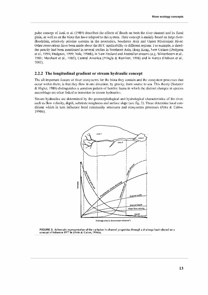
2.2.2 The longitudinal gradient or stream hydraulic concept

The all-important feature of river ecosystems for the biota they contain and the ecosystem processes that

occur within them, is that they flow in one direction, by gravity, from source to sea. This theory (Statzner

& Higler, 1986) distinguishes a zonation pattern of benthic fauna in which the distinct changes in species

assemblage are often linked to transition in stream hydraulics.

Stream hydraulics are determined by the geomorphological and hydrological characteristics of the river,

such as flow velocity, depth, substrate roughness and surface slope (see fig. 3). These determine local con-

ditions which in turn influence local community structures and ecosystems processes (Petts & Calow,

1996b).

FIGURE 3. Schematic representation of the variation in channel properties through a drainage basin (based on a concept of Schumm 1977 in (Petts & Calow, 1996b).

State of the Art

14

2.2.3 The four-dimensional nature of lotic ecosystems

The four-dimensional concept presented by Ward (1989) is mentioned here as it introduced the temporal

scale. Upstream-downstream interactions constitute the longitudinal dimension, as expressed by the longi-

tudinal gradient or the RCC. The lateral dimension includes interactions between the channel and riparian/

flood plain systems, which is more related to large river and does not concern the studied headwater sys-

tem. Significant interactions also occur between the channel and contiguous groundwater, the vertical

dimension through the hyporheic zone (sub-benthic habitat of interstitial spaces between substrate parti-

cles in the stream bed). The fourth dimension, time, provides the temporal scale. Lotic ecosystems have

developed in response to dynamic patterns and processes occurring along these four dimensions.

2.3 Disturbance concept

Disturbance is regarded by many stream ecologists as playing a central role in determining the structure of

stream communities (e.g. Resh & Rosenberg, 1989; Lake, 2000). Disturbance is defined by (Stanford &

Ward, 1983) as: “any stochastic event which forces normal system environmental conditions substantially

away from the mean”. Severity of disturbance includes both frequency (or timing) and duration.

For Lake (2000), perturbation describes the combination of cause and effect: disturbance becomes the

cause of a perturbation, and response becomes the effect of the disturbance. Disturbances may be charac-

terised by their temporal patterns: thus, we have pulses, presses and ramps (see fig. 4). Pulses are short-

term and sharply delineated disturbances (e.g. floods). Presses may arise sharply and then reach a constant

level that is maintained (e.g. sedimentation after landslides or after fires), mostly resulting of human activ-

ities (e.g. dams, channelisation, heavy metal pollutants). Ramps occur when the strength of a disturbance

steadily increases over time (droughts as “creeping disaster”, increasing sedimentation of a stream as its

catchment is cleared, or the incremental spread of an exotic organism).

FIGURE 4. Three types of stream disturbance (A: Pulse, B: press, C: ramp) distinguished by temporal trends in the strength of the disturbing force. Note that ramp disturbances may level off or increase steadily throughout the period of observation (Lake, 2000)

The response of the system has often been confounded with the disturbance itself. It can also take the form

of pulse, press or ramp response. The characterisation of the response is linked with the qualities of resist-

ance, a measure of the capacity of the system to withstand a disturbance, and resilience, a measure of the

capacity of the system to recover from disturbance.

A number of hypotheses have been proposed to explain how disturbance affects diversity. One of these

hypothesis was developed by (Connell, 1978), as the “Intermediate Disturbance Hypothesis”. This hypoth-

Time Time TimeStrength of disturbing force

Strength of disturbing force

Strength of disturbing force

Disturbance concept

15

esis suggested that highest diversity is maintained at intermediate scales of disturbance (figure 5) and is a

consequence of continually changing conditions. This theory was proposed for plants (tropical rainforests)

and sessile animals (coral reefs). The hypothesis is based on the argument that ecological communities sel-

dom reach an equilibrium state, in which the competitively superior individuals will continually set back

the process of competitive elimination by opening space for colonisation by less competitive individuals.

(Connell, 1978) concluded by underlining that “although tropical rain forests and coral reefs require distur-

bances to maintain high species diversity, it is important to emphasize that adaptation to these natural dis-

turbances developed over a long evolutionary period”.

FIGURE 5. The Intermediate Disturbance Hypothesis (Connell, 1978).

The Intermediate Disturbance Hypothesis has been studied in stream ecology, disturbance regarded as

playing a central role in determining the structure of stream communities (e.g. Lake, 2000; Matthaei &

Townsend, 2000; Palmer et al., 1992; Reice, 1985; Resh et al., 1988; Robinson & Rushforth, 1987; Stan-

ford & Ward, 1983). It also has important practical implications for the maintenance of biodiversity, of

which species richness is the most basic component (Townsend & Scarsbrook, 1997). It appears that inter-

mediate level of disturbance induced by the flooding regime may lead to higher levels of alpha and beta

diversity (Ward, 1998). However, according to Death (2002), there appears to be no widely accepted

model that can be used to predict link between diversity and disturbance, nor is there much understanding

of the mechanisms behind that relationship.

2.3.1 Documented impacts of logging activities in South-East Asian tropical forests

As the impacts of logging activities have been the subjects of a pletoria of studies, studies mentioned there-

after are focused on South-East Asian tropical forests.

In Borneo, primary lowland forests exhibit a high density of harvestable trees (23 trees/ha > 50 cm diame-

ter and 16 trees/ha >60 cm diameter) (Sist & Nguyen-Thé, 2002). As a result, these forests are considered

as highly productive compared to other countries (table 1) and harvesting intensity commonly exceed 100

m3/ha representing more than 10 trees/ha (Sist et al., 2002). In Africa and South America, harvested vol-

umes generally remain below 50 m3/ha (Sist et al., 1998).

Low

high

Diversity

Disturbances frequent infrequentSoon after a disturbance long afterDisturbance large small

State of the Art

16

There have been several studies on the effects of logging in southeast Asian rainforests focusing mainly on

the amount and types of damage sustained by the residual stand immediately after logging, and the degree

to which the forest floor was disturbed by roads and tracks (e.g. Nicholson, 1958; Fox, 1968; Tinal and

Palenewen, 1978; Abdulhadi et al., 1981; Borhan et al. 1990; as cited by Cannon et al., 1994). These stud-

ies revealed that, as everywhere in the tropics --but mainly in Southeast Asia and in South America-- apart

from exceptions, logging of natural forest is rarely sustainable.

Loss of biodiversity and loss of structure of residual stands. The unlogged lowland forest is species-rich,

but the commercial species dominate, comprising 70% of total precut basal area. Cannon et al. (1998), in a

study in West Kalimantan (Indonesian Borneo), found that, by removing 62% of dipterocarps basal area

and 43% overall, logging reduced both tree density and the number of tree species per ha, for both large

and small trees. For all trees > 20 cm in diameter, density fell by 41% and the number of species per plot

by 31%. The percentage of lowland forest classed as moderately to heavily disturbed ranged from 70 to

84%. Other studies of residual stand include Haeruman (1978); Rosalina (1986); Tinal and Palenewen

(1978); Abdulhadi et al. (1981); as cited by Cannon et al. (1994).

Logging activities, apart from log cutting and felling, include all associated infrastructure such as skid

trails, roads, river landings, etc., which imply major movements of soils. These infrastructure elements can

be major factors of soil erosion if improperly constructed or maintain. In Indonesia, there is ample evi-

dence that typical timber concession apply poor road construction, maintenance and drainage practices.

Additionally, inadequate planning and layout of logging blocks with excessive amounts of improperly

designed skid trails are frequent (Klassen, 1999; Sève, 1999; pers. observ.). Erosion can also inflict direct

damage to infrastructure such as roads and bridges, and human settlements in the form of mud flows and

flooding. The life span of hydroelectric and irrigation dams can be considerably reduced as a result of ero-

sion (Sève, 1999).

Impact of logging on rivers and macroinvertebrates. Since 1980, many studies have been carried out on

logging or forest conversion effects on hydrology and sediment yield in Malaysia (Zulkifli et al., 1990;

Lai, 1992; Malmer, 1990; Law et al., 1989: as cited by Douglas et al., 1993; Douglas et al., 1992). Logging

and ground clearance increased river sediment by two to fifty times in Danum Valley (North Borneo)

(Chappell et al., 1999). Soil erosion can have an impact on water quality, primarily through suspended sol-

ids, but also by increasing biochemical oxygen demand (BOD), all of which can affect downstream users

of drinking water (Sève, 1999). Seasonal flow patterns can also be affected as a result of altering the vege-

tative cover of watersheds.

In temperate climate, deposited sediment affected the structure and function of benthic macroinvertebrates

communities by increasing substrate embeddedness and altering substrate particle-size distribution (Culp

et al., 1983; Erman & Erman, 1984; Minshall, 1984; Lenat et al., 1981), producing a reduction in habitat

TABLE 1. Harvesting intensity in some tropical countries.

CountriesNo. of trees

per ha (m3/ha)References

Brazil 4 to 8 Barreto et al., 1998; Johns et al., 1996; ; Winkler, 1997 as

cited by Boltz et al., 2003; Holmes et al., 2002

Ecuador (northwest) 8 Montenegro, 1996 as cited by Boltz et al., 2003

Guyana 3 to 16 Armstrong, 2000; Van der Hout, 1999: as cited Boltz et al.,

2003

Bolivia (Santa Cruz) 4.32 (12.1) Jackson et al., 2002

Indonesia > 10 Dykstra and Heinrich, 1996; Bertault & Sist, 1997; Sist et

al., 2002

Review of existing literature and information on Indonesia related to the study

17

quantity and quality. A small increase in sediment may reduce macroinvertebrate population densities

because of a reduction in habitat space; however, community structure may not change. Alternatively, as

deposited sediment increases, densities may increase, and alterations in community structure and diversity

can occur. Zweig & Rabeni (2001) underlined that changes in macroinvertebrate fauna caused by depos-

ited sediment were difficult to isolate and quantify because they often accompany other changes in the

stream, such as removal of riparian vegetation, alterations in flow and temperature regimes and nutrient

enrichment.

But for Borneo, there is a lack of data on most lowland rivers to ascertain whether the rapid expansion of

logging has caused channel changes which could potentially affect the lives of the riparian communities,

including the macroinvertebrates (Douglas et al., 1993). Martin-Smith et al. (1999) studied the mecha-

nisms of maintenance of tropical freshwater fish communities in the face of selective logging activities in

Danum Valley (Sabah, Malaysia). They found that fish communities from headwater streams showed few

long-term changes in species composition or abundance, but short-term (<18 months) absence of decrease

in abundance.

Evidence suggests that in tropical rainforest environments, selective logging may lead to an increased sus-

ceptibility of forests to fire. Siegert & Hoffmann (2000) assessed the extent of the fire-damaged area and

the effect on vegetation in East Kalimantan following the 1997-98 fires associated with El Niño phenome-

non. A total of 5.2 +/- 0.3 million hectares including 2.6 million ha of forest was burned. Forest fires pri-

marily affected recently logged forests; primary forests or those logged long ago were less affected.

Human impact by road construction and logging, as well as man-made fires has accelerated the fragmen-

tation in various vegetation types. A study on the effect of fragmentation on the behaviour of Bornean gib-

bons emphasizes that the fragmentation of habitats causes a slow, but sure, increase in the number of

species facing extinction through a decrease in genetic diversity that enables adaptation to environmental

change, although the effects are not apparent immediately (Oka et al., 2000).

As a result of these poor logging practises, Reduced Impact Logging (RIL) has been developed. Previous

studies of RIL in Southeast Asia have demonstrated that damage to the tropical forests can be significantly

reduced by applying simple techniques of forest management planning, including pre-harvesting surveys,

pre-mapping of timber trees, vine cutting, design and location of skid trails before logging and directional

felling. Although most current harvesting system throughout South-East Asia encompasses almost all

these RIL rules, they have not been applied on a larger scale for numerous reasons. These include lack of

technical knowledge, minimal control of harvesting practices and the perceived high economic cost of

RIL.

2.4 Review of existing literature and information on Indonesia related

to the study

2.4.1 Politics and Forestry in Indonesia

Indonesia’s territory today is defined by the boundaries of the former Dutch East Indies, as a result of

Dutch colonisation which began in 1602. In 1942 the Japanese conquered the Dutch East Indies, and after

Japan’s defeat Indonesian nationalists under the leadership of Sukarno declared independence in August of

1945. Sukarno became President and a 15 year period of political instability and economic decline fol-

lowed, during which there were numerous verbal conflicts with the Netherlands and a military conflict

with Malaysia. In 1965 a failed coup d’état led by a group of military officers occurred with the support of

State of the Art

18

the Indonesian Communist Party and China. The coup was crushed and as many as 750,000 of the support-

ers of the communist party were killed. The coup marked the end of Sukarno’s presidency and in March

1966 a “New Order” was established. In March 1968, Suharto became president. When the New Order

was established, the government defined three economic objectives: stability, growth and equity, to be

achieved through a series of 5-year development plans (REPELITA), applicable to the public and private

sector. The results were successful in several ways and the economy grew at an average rate of 6.8% from

1965 to 1995 and became increasingly export-orientated. In 1995, oil and gas accounted for 23% of

exports by value, followed by timber products (10%) and textiles (6%). Poverty declined since the 1960s

but substantial inequalities of income remain, as well as widespread corruption.

A regional economic crisis in Southeast Asia which began in 1997 had major political and economic

impacts on the country. In May 1998, President Suharto resigned and was replaced by his Vice-President

Mr. Habibie. In mid-1998, 50 million Indonesians were living in poverty largely due to price increases as a

consequence of the decline in the value of the rupiah (80% of it value). During parliamentary elections in

1999, Megawati Sukarnoputri’s party won must of the votes, a third of the total, in a race between dozens

of parties. But Muslim cleric Abdurrahman Wahid outmanoeuvred Megawati when legislators chose the

president a few months later. Those legislators sacked Wahid for incompetence in July 2001, allowing

Megawati to move up from the vice-president's post. She was appointed as Indonesia’s fifth president.

Figure 6 summarises the Forestry in Indonesia for the last 30 years. More information on the detailed proc-

esses can be found in the following sources: Elliott (2000), a review of Forestry sector policy issues (Sève,

1999) and a guideline concerning the natural production forest management (NRMP, 1993) both supported

by the Natural Resources Management program, and a World Bank report (WorldBank, 2001).

2.4.2 Importance of forestry in the Indonesian economy

Forestry in Indonesia has changed rapidly over the last thirty years. Until the late 1960s, commercial tim-

ber production was mostly limited to teak plantations in Java. Starting in the early 1970s, large areas of

forests in the “outer islands” (especially Kalimantan and Sumatra) were allocated by the government to the

private sector in the form of 20-year timber concessions (Elliott, 2000). Indonesia started the 1980s as a

log exporter and, because of a ban on log exports (1991-1996) to promote domestic processing, ended the

decade as a major plywood exporter. With the growth of the plywood industry, the political and economic

influence of the private sector increased. The development of the pulp and paper industry is a current prior-

ity with substantial investments being made in plantations and pulp and paper mills, partly encouraged by

tax-write-off (Elliott, 2000).

Annual log production increased from 1.4 million cubic metres in 1960 to 33 million in 1996. Log produc-

tion in East Kalimantan has been about 3-5 million m3 per year during the past 20 years, which account for

about 20% of the entire production in Indonesia. The seventh Development Plan (for the years 2000 to

2004) has set a log production target of 57.2 million m3 per year for the whole of Indonesia. Although the

plan will be reassessed because of the economic crisis in 1997-98, the productive capacity of timber

processing mills and upgrading the living standards of the country will require more log production than

the present amount of about 25 million m3/year (Fatawi & Mori, 2000).

Until the mid-1990, resource-related exports from the natural forest were an engine of economic growth.

Forest-based exports (plywood, furniture, and pulp) rose from around $200 million in the early 1980s to

more than $ 9 billion per annum in the mid-1990s. In 1997, total output from forest-related activities was

about $20 billion (10% of GDP). Forest-related employment were about 800,000 jobs in the formal sector,

and many more than this engaged in activities in the non-traded forest products sector. Royalties and other

government revenues from forest operations exceeded $1.1 billion per annum (WorldBank, 2001).

Review of existing literature and information on Indonesia related to the study

19

FIGURE 6. Summary of main characteristics of forestry sector in Indonesia since 1967

• Constitution and Basic Forestry Law of 1967 stated that State controlled land, water

and natural resources

• timber concessions are granted for 20 years, but tree-harvesting cycles are every 35

years => no security of tenure

• a high priority is given to timber production

• cartel and monopoly on wood production by Suharto and a few members of his gov-

ernment and family, with centralisation of Ministry of Forestry in Jakarta (Barr, 1998)

• development of hundreds of regulations and decrees

=> directives detailed, but not always consistent with one another

=> high pressure on forest concession who spend their time on administration instead

of forest management

• corruption at all government and local levels

• illegal logging

• unsustainable forest management

Decentralisation started in 1999 with following basic changes in forestry sector:

• all local resources, including forestry activities, are under the supervision of the

local government

• local population recover their rights on the uses of their natural resources

The reality since the forestry law of 1967

As a result

Decentralisation as a solution?

But, so far.....

• new forestry laws ambiguous and lack essential implementing guidelines, which lead to

confusion with old existing laws

• decentralisation process too rapid, no time to build human capacities at regional govern-

ment level for land-use planing, forest management, conservation area and the other new

tasks

• land ownership to be determined between the local population arise conflicts

• acceleration of environmental degradation (logging activities increase up to 3 times offi-

cial logging (Casson & Obidzinski, 2002)) to money natural resources, by taking advan-

tages of the lack in government controls

State of the Art

20

Recent trends in tropical timber production, excluding plantations, show a decrease in the Asian-Pacific

region’s share of global production by approximately 30% from 1992 through 1999. This decrease can be

attributed to the Asian economic crisis which also affected Indonesia’s plywood exports to key markets

such as South Korea and Japan. The Ministry of Forestry estimated that plywood export revenues in 1997

were 25% lower than in 1996 (Fatawi & Mori, 2000). Production in the Latin America-Caribbean region,

which is dominated by South American producers, increased 15.8% over the same period (ITTO in Boltz

et al., 2003).

2.4.3 Deforestation and forest degradation

Concerns began to be raised about deforestation and forest degradation in Indonesia by Indonesian NGOs

and foreign scientists and observers in the mid-1980's, at a time when international concerns about loss of

tropical forests, and the role of the international timber trade in this, were increasing. One of the catalytic

events was the large forest fires in Kalimantan in 1982 and 1983.

There has been considerable controversy concerning the causes of deforestation, with analysts divided

over the direct and indirect responsibilities of logging, shifting cultivation, land clearing for plantation

(both forest and non-forest) and transmigration. Land clearing is performed by various methods of which

the use of fire is one of the most important. Approximately, one tenth of the annual rate of deforestation is

attributed to logging in natural forests (Sève, 1999). In general, concession operations are characterised by

inadequate planning prior to harvesting procedures and systems, poor road location and design, rigid log

specifications, and excessive wood residue remaining in the forest following harvesting. These are all fac-

tors that contribute to the degradation of forest ecosystems.

In a recent study from Achard et al. (2002), the changes in humid tropical forest cover from satellite

remote sensing imagery were estimated. Southeast Asia had the highest annual percentage deforestation

rate (0.91%), and Africa lost its forests at about half the rate of Southeast Asia. Latin America showed the

lowest percentage rate, but at a rate of 2.5 x 106 ha year-1, the annual loss of forest area was almost the same

as the loss estimated for Southeat Asia (2.5 +/-0.8 x 106). These estimates represent only the proportion of

degradation identifiable using remote sensing, which does not include processes such as selective logging

as well as the fire events in Indonesia in 1997-1998.

According to Cannon et al. (1994), of Indonesia’s closed forests, 61% has been designated as production

forest and allocated to logging concessionaires. By 1985, 51% of the production forest had been logged.

Estimates of the annual deforestation rate diverge widely, partly because of the use of different definitions

and partly because of weak data, ranging from 600,000 ha (Sève, 1999) to 2.4 million ha per year. Some

TABLE 2. Forest cover, forest loss and logging activities: comparison between the whole country, Kalimantan and East

Kalimantan province. Sources from Fatawi & Mori (2000) and WorldBank (2001) report.

Indonesia Kalimantan East Kalimantan

1985 1997 1985 1997 1985 1997

Total land area (ha) 190’905’100 189’702’068 53’583’400 53’004’002 19’721’000 19’504’912

Forest area (ha) 119’700’500 100’000’000 39’986’000 31’512’208 17’875’100 13’900’000

Forest % 62.7 50.1 74.6 59.5 90.6 71.3

Forest loss (%) 16.5 21.2 22.2

Forest loss ha/year 1’641’708 706’149 331’258

Logging concessions (ha) 37’500’000 11’800’000 4’600’000

Timber estates allocated (ha) 6’400’000 3’100’000 1’300’000

Timber estates realised (ha) 2’400’000 900’000 500’000

Review of existing literature and information on Indonesia related to the study

21

numbers are presented in table 2.In 1968, forests covered an estimated 77% of Kalimantan (41.5 million

ha), which was about 34% of the total forest area of Indonesia at the time. By 1997 forest cover was esti-

mated at 60% (31.5 million ha). In East Kalimantan, total land area is estimated between 19’720 and

21’140 km2, depending on the source (RePPProt/WorldBank, 2001) versus MoF/Fatawi & Mori, 2000).

But in both figures, forest land covers over 91% of the territory before 1980. This forest cover drop at 71%

in 1997 according to MoFEC numbers (Table 2). East Kalimantan have the highest rate of conversion

compared to the other Indonesian provinces, with the lost of 10 million ha within less than 30 years

(WorldBank, 2001).

The fires, as mentioned in the previous sub-chapter 2.3.1., participated in 1992-93 and in 1997-98 to the

forest degradation by huge amounts of hectares of forest burnt in Kalimantan (2.6 millions ha of forest).

On top of that, by the year 2001, illegal logging was thought to be one of the most critical threats to forest

capital, accounting for 50-70% of total log production. Casson & Obidzinski (2002) suggested that “illegal

logging” is not a simple case of criminality, but a complex economic and political system involving multi-

ple stakeholders. It should be viewed as a dynamic and changing system deeply engrained in the realities

of rural life and regional autonomy created a supportive environment for it.

2.4.4 Environmental conservation and protection

Indonesia has a number of legislative texts that deal directly with environmental protection. Among these,

the most important are: a) the Management of the living environment law of 1982; b) the law on the Con-

servation of the living environment and its ecosystem of 1990; c) the Spatial use management law of 1992

and d) the law on the management of the living environment of 1997. All these laws, which are phrased in

a similar way and support one another, constitute a legal framework that:

• requires that natural environment be managed in a sustainable fashion

• establishes obligations to exercise a function of environmental protection to holders of rights on

land and water

• sets out principles of land use

• defines environmental damages

• creates the legal basis for environmental audits

• determines penalties for environmental damages

Additionally, regulations require the preparations for environmental management and monitoring plans for

the renewal of natural forest concessions, the awarding of new natural forest and the development of tim-

ber plantations (MOFEC decree). Despite this detailed legal and regulatory structure, environmental dam-

age associated with forestry operations continue and may be increasing as the effects of newly opened

logging blocks accumulate with those of previously harvested area (Sève, 1999).

2.4.5 Limnology and aquatic communities

According to Lehmusluoto et al. (1999) and Dudgeon (1992, 1995), limnological information of the Indo-

nesian freshwater, lake, reservoirs, wetlands, swamps and river is limited. There have been only a few

major limnological studies, such as the Sunda-Expedition in years 1928-1929, covering Sumatra, Java and

Bali, and a great number of sporadic studies, restricted in area and depth, from the 1970s, 1980s and 1990s,

and the most recent Expedition Indodanau which covered the major lakes and reservoirs in Sumatra, Java,

Bali, Lombok, Flores, Sulawesi and Irian Jaya (Lehmusluoto et al., 1999). A status of limnology in Indo-

nesia has been presented by Nontji (1994) as well as a review of current knowledge of Indonesia’s major

freshwater lakes by Giesen (1994).

State of the Art

22

There are more than 400 freshwater fishes known in Indonesia, mostly Cyprinidae, Cyprinodontidae,

Balitoridae, Bagridae, Siluridae, Gobiidae, Belotiidae, Aplocheneilidae, Channidae, Clariidae, Poccillii-

dae, Cichlidae, Helostomatidae, and Anabantiadae. In Kalimantan and Sumatra, there are more species

than in Java, but the density is greater in Java. Java’s native fish are both less abundant and less diverse

than they were because of loss of forest, water pollution, sediment dredging and damming (Lehmusluoto et

al., 1999). In their article, Lundberg et al. (2000) proposed an overview of recent ichthyological discovery

in continental waters. This paper includes studies made in tropical Asia (the Oriental Realm, extending

from the Indus Basin eastward to South China and to the Mollucas in Indonesia) and records works from

Kottelat (e.g. Kottelat & Whitten, 1996a and b) and others.

Aquatic insect diversity and ecology in tropical Asian streams has been summarised in a recent book

(Dudgeon, 1999). Lehmusluoto et al. (1999) summarised the available information concerning macroin-

vertebrates and benthic algae in Indonesia, but mentioned that information on fungi, bacteria, zooplankton,

benthos, periphyton, and littoral and surface vegetation is not adequate enough for a review. Bits and

pieces of information may be found from the 8'000 pages of reports of the Sunda-Expedition in “Archiv

für Hydrobiologie Supplement” volumes published in 1931-1958, mainly on taxonomy (about 1100 new

species reported by Ruttner (1931, 1932, 1940, 1952) and Thienemann (1930, 1931, 1932, 1959), on peri-

phyton (Nurbakti, 1991; Sulisyo, 1991), benthos (Sylviani, 1992), macroinvertebrates (Rumpoho, 1987,

Kusjantono, 1991; Kadarusman, 1991), and molluscs (Samanya, 1989), on biology of various lakes

(Eyanuer et al., 1981; Universitas Andalas, 1984; Universitas Cendrawasih, 1984), and on ecology by

Whitten et al. (1987a,b, 1996) and Green et al. (1976, 1978, 1995). All these references can be found in the

article written by (Lehmusluoto et al., 1999) and the one concerning periphyton, benthos and macroinver-

tebrates are written in Indonesian language and could not be found.

In this study, as the mayflies (Ephemeroptera) could be identified to generic level, some information based

on Sartori et al. (in press) are provided. The following litterature references can be found in this article.

The first species described were Rhoenanthus speciosus (Potamanthidae) and Atopopus tarsalis (Heptage-

niidae) at the end of the 19th century (Eaton, 1881). Ulmer's famous work on mayflies of the Sunda

islands1 focused mainly on Java and Sumatra, with sparse data on Borneo (Ulmer, 1939). Nevertheless, he

described 9 new genera and 12 new species from this island. Since that time, a few contributions have

brought some new data (Demoulin, 1953, 1954; Peters, 1972; Allen & Edmunds, 1976; Müller-Liebenau,

1984; Grant & Peters, 1993; Wang & McCafferty, 1995; Wang et al., 1995). The only supraspecific mod-

ern synthesis of mayflies found on the Sunda Islands has been the publication by Edmunds & Polhemus

(1990), as well as the recent survey of Ephemeroptera from the Oriental region (Soldán, 2001). At the end

of the 20th century, 35 genera and 44 species were recorded.

Considering the available information, our study will contribute to the scientific knowledge in tropical

ecosystems, not only on the evaluation of landscape and ecological water quality indicators, but also on

basic knowledge on the stream biota itself (habitat and macroinvertebrates fauna) and on the relationship

about logging activities and the stream ecosystem.

1. group of islands extending from the Malay Peninsula to the Moluccas southeast of the Asiatic mainland toward New Guinea. They include the Greater Sundas (Sumatra, Java, Borneo, Sulawesi, and adjacent smaller islands) and the Lesser Sundas (Bali, Lombok, Sumbawa, Sumba, and Flores, Timor, Alor, and adjacent smaller islands).

��

&+$37(5�� ��������

This chapter presents the geographic location of the study area inside a state-ownedtimber concession, Inhutani II. Management in this timber concession is described.Available information on natural features includes climate, geology, land systemsand associated soils, hydrology, vegetation and fauna are presented.

�����*HRJUDSKLF�ORFDWLRQ

The research area was located in the Borneo island, on the Indonesian part covering73% of the total island area, more precisely, in East Kalimantan. Borneo is the thirdlargest island in the world (after Greenland and New Guinea) with approximately740’000 km2.

In East Kalimantan, the study area was more precisely located in Malinau provincewhich was previously part of Bulungan province. Bulungan was divided in October1999 into three smaller provinces : Bulungan (18’000 km2), Malinau (42’600 km2)and Nunukan (13’800 km2).

The study area itself, covering 8500 ha, was located at latitude 116°30'E and longi-tude 3°00'N, inside a state owned concession, Inhutani II (see figure 7 for location).The study area was usually reached by air from Jakarta to Balikpapan, then fromBalikpapan to Tarakan and finally from Tarakan to Malinau using a local air line(DAS) which takes half an hour. These flights operated twice a week when weatherallowed it. The usual transportation for local population was by boat on the riverSesayap. About 4 to 5 hours were necessary to go upstream from Tarakan to Mal-inau town with a speed-boat. From there, a logging road led to the camp inside theconcession within 3.5 to 4 hours drive (~90 km). The duration of the journey mostlydepended on the water level, as the Rian river had to be forded to reach the camp.The closest village, Long Loreh was about 30 minute drive from the camp. Theentire journey, from Jakarta to the study area, was usually made over two to threedays.

6WXG\�$UHD

��

),*85(��� 3DUWLDO�PDS�RI�6RXWK�(DVW�$VLD�ZLWK�ORFDWLRQ�RQ�%RUQHR�,VODQG�RI�VWXG\�DUHD�LQ�EOXH�

�����,QKXWDQL�,,�WLPEHU�FRQFHVVLRQ

PT Inhutani II Unit Malinau, a state-owned company, started its logging activities based on the Ministry ofForestry decree No. 64/Kpts-II/1991 issued on January 30, 1991. The area allocated to the concession cov-ers 48’300 ha, located 116°-116°40’E latitude and 2°52’-3°14’ N longitude (see figure 8). PT Inhutani IIconcession is surrounded by PT Inhutani I and Bhakti Barito on the north side, Intracawood (ex-PT Inhu-tani I) on the east side, PT Meranti Sakti on the west side and by a protected forest, Bukit Condong on thesouth side. The 48’300 ha includes 14’180 ha of limited production forest, 23’890 ha of permanent produc-tion forest and 10’230 ha of unproductive land.

The concession started to log in 1991 in the north-east of the allocated area. Some of the firsts cuttingblocks are very distant from each others. In order to minimise the spatial effect, we decided to remain intwo watershed which contained most of the previously cut blocks. On these two watershed, the Seturanand the Rian, we were thus able to find a chronological sequence from logged in 1995 up to logged in2000. A whole portion of the watershed, corresponding to cutting block logged in 1997 was inaccessibledue to a broken bridge and was avoided.

Sabah

Sarawak(Malaysia)

Kalimantan(Indonesia)

Java

Jakarta

Tarakan

(Malaysia)

Malinau

SumatraSamarinda

Balikpapan

studyarea

Philippines

Sulawesi

Borneo

BruneiMalaysia

South China Sea

Indian Ocean

,QKXWDQL�,,�WLPEHU�FRQFHVVLRQ

��

),*85(��� /RFDOLVDWLRQ�RI�,QKXWDQL�,,�FRQFHVVLRQ��EROG�OLQH��DQG�RWKHU�VXUURXQGLQJ�FRQFHVVLRQV��:KLWH�DUHDV�DUH�ODQG�ZKLFK�LV�QRW�DOORFDWHG�IRU�LQGXVWULDO�IRUHVW�SODQWDWLRQ�RU�IRUHVW�FRQFHVVLRQ��RU�ODQG�ZKLFK�DUH�RQ�UHQHZDO�SURFHVV�DW�WKH�WLPH�RI�WKH�PDSSLQJ��6RXUFH��3HWD�SHUNHPEDQJDQ�SHQWDDQ�EDWDV�DUHDO�NHUMDK�+3+�������������GLJLWLVHG�DQG�XSGDWHG�E\�*7=��6DPDULQGD��2ULJLQDO�VFDOH�������¶����

Inhutani II operated under the Indonesian Selective Cutting and Planting Silvicultural System (TPTI:Tebang Pilih Tanam Indonesia), which replaced the previous selective cutting system (TPI: Tebang PilihIndonesia) in 1989. The eleven steps which make up the TPTI system are summarised in table 3.

This TPTI system is designed to produce a sustainable supply of timber on a growing cycle of 70 yearswith a harvest every 35 years. Only trees over 50 cm diameter may be harvested in production forest andtrees over 60 cm diameter in limited production forest. Logging is done in blocks, with each concessionbeing divided into 35 annual blocks. The Annual Allowable Cut for each block is set by the Ministry ofForestry. At least 25 commercially valuable trees with diameters between 25 and 50 cm must remain afterlogging and post-logging enrichment planting is required. In principle, these requirements imply thatapproximately one cubic metre of timber would be harvested per hectare annually. Planning requirementsare stringent and complex, with concessionaires being required to submit annual management plans, vari-ous work plans, environmental impact assessments and community development plans (Elliott, 2000).

80 0 80 160 Kilometers

1

(:

6

Protected forest

Forest concession

Industrial forest plantation

Tarakan

6HVD\DS�ULYHU0DOLQDX

/RQJ�/RUHK

FDPS

,QWUDFDZRRG

,QKXWDQL�,

0HUDQWL�6DNWL

%XNLW�&RQGRQJ

6WXG\�$UHD

��

Concessionaires pay a variety of royalties, fees and taxes including a volume-based reforestation fee whichgoes into a reforestation fund managed by the Ministry of Forestry. This fund is supposed to be used tofund reforestation activities but there have been a number of cases of Presidential misuse (Elliott, 2000).

The basic assumption of this TPTI system is that through its application, a perpetual supply of raw materialto the forest industry can be assured without compromising the protective functions of the forest or thebasic resources of soil and water (NRMP, 1993). The system assumes that the following conditions can besatisfied:

• minimum stocking of nucleus trees2 before logging is 25 trees/ha. Nucleus tree must be 20 to 49 cmdiameter at breast height and of commercial species

• the felling cycle is set at 35 years with an assumed diameter increment of 1cm per year

• tolerable loss of nucleus trees during initial exploitation is not stated but 10% could be consideredas reasonable

• mortality of nucleus trees during the cycle is not acknowledged. FAO studies suggest a loss of 1%per year.

A long term management plan (RKPH: Rencana Kerja Pengusahaan Hutan) on 20 years is prepared by theconcessionary. This plan should report past and future management activities including the eleven stepsfrom TPTI guidelines, as well as forest product, marketing, protection, development of local communities,proposals for research and conservation, 20 year cash flow, profit and loss statements and production pro-jections (amongst others). The RKPH divides the concession area into seven equal blocks, each covering afive year working period (RKL: Rencana Kerja Lima Tanhun), such as in figure 9. This covers the 35 yearscycle, but the concession area is granted for 20 years. Every RKL is divided into 5 equal blocks for annualworking plan (RKT: Rencana Kerja Tahunan), each divided in 100 ha plot (petak in Indonesian language).

Hundred percent inventory of all commercial species with diameter >20 cm is carried out during step 2(table 3). Beyond this distinction, the enumeration provides no qualitative assessment of recoverable tim-

7$%/(����737,�DFWLYLW\�VFKHGXOH��QXPEHU�RI�\HDUV�EHIRUH�IHOOLQJ��7������������DQG�DIWHU�IHOOLQJ��7����XS�WR�����

1E 737,�DFWLYLW\7LPH�UHODWLYH�WR�IHOOLQJ��7�

1 Working area organisation (boundary) T -3

2 Inventory before felling T -2

3 Infrastructure establishment (roads) T -1

4 Felling (logging activities) T

5 Liberation (removing of bushes, low growing vegetation,.) T +1

6 Inventory of residual stand T +1

7 Seedling procurement T +2

8 Planting / enrichment T +2

9 Tending/ first phase T +3

10 Subsequent tending (a) liberation T +4

(b) thinning T +9, 14, 19

11 Protection and research continuously

2. commercial trees species to be left for the next cutting cycles. They have to be clearly marked in the field.

,QKXWDQL�,,�WLPEHU�FRQFHVVLRQ

��

ber volumes. The results are summarized in an inventory report (Laporan Hasil Cruising, LHC). Commer-cial target species are drawn from this inventory and form the basis for all further calculations andharvesting control. The RKPH includes a calculation of the Annual Allowable Cut (AAC):

where A = area of available forest, V= average volume of commercial species per hectare (50 cm diameterand up) from the inventory and 35 = cutting cycle.

Since the AAC equation does not reflect loss due to waste, breakage, decay or other losses, two correctionfactors have been introduced which are used to obtain the Annual production quota (JPT) as follows: JPT =AAC x 0.56. This consists of a "utilisation factor" (0.7) and a "safety factor" (0.8). The resulting volume isspecies-specific. All subsequent production occurs within this species-specific target figure and within thedesignated annual harvesting area. This volume per area limit becomes the cut-control mechanism withinwhich Inhutani is relatively free to operate. Since there are no controls on the level of utilisation during thelogging activities, the company has no incentive to make use of the volume cut and will tend to highgradethe stand level until it achieves its annual production quota (JPT) or until it reaches its annual harvest areatarget (NRMP, 1993).The annual cutting area set for Inhutani II concession consists of nine petak. Figure 9presents the RKL 5-years cutting blocks. Production data was obtained for the past nine years which com-pares the approved annual production target and the actual annual production (see table 4).

Inhutani monitors its production closely and submits periodic production reports to the Ministry of For-estry. It is not uncommon for Inhutani to re-enter a specific petak during the course of the production yearif it needs additional volume to meet the annual production target. Under-performance against this target,can carry a penalty generally consisting of a reduction in the next years target, although there is no evi-dence that this has ever occurred in the Inhutani II operation.

7$%/(����$UHD�DQG�YROXPH�WDUJHW�IRU�HDFK�\HDU�DQG�DFWXDO�DUHD�DQG�YROXPH�ORJJHG��'HSHQGLQJ�RQ�ZKLFK�,QKXWDQL�,,�

UHSRUW�DUH�FRQVXOWHU��QXPEHUV�DUH�GLIIHUHQW��VXFK�DV�LQ�FROXPQ�©DQQXDO�SURGXFWLRQª�YHUVXV�©RWKHU�DQQXDO�SURGXFWLRQª�

<HDUV7DUJHW�DUHD��KD�

DUHD�ORJJHG��KD�

DQQXDO�SURGXFWLRQ�WDUJHW��P��

DQQXDO�SURGXFWLRQ�

�P��

7LPEHU�TXDQWLW\��P��KD�

RWKHU�DQQXDO�

SURGXFWLRQ�P��

6ROG�SULFH��US�P��

1991-1992 1’000 900 30’400 26’421 29.35 28’747 88’532

1992-1993 900 850 29’000 26’430 31.09 27’318 85’845

1993-1994 900 600 39’160 20’720 34.5 20’656 154’202

1994-1995 900 600 24’000 22’875 38.12 42’290 122’982

1995-1996 1’100 1’000 41’200 33’240 33.24 30’018 115’389

1996-1997 1’100 900 37’535 17’631 19.5 19’975 191’371

1997-1998 775 450 26’444 22’757 50.5 30’374 176’893

1998-1999 904 635 30’952 20’604 32.4 16’121 311’234

1999-2000 925 26’183 25’018 387’104

2000-2001 25’575 572’337

AACA V×

35-------------=

6WXG\�$UHD

��

),*85(��� )LYH�\HDUV�FXWWLQJ�EORFN��5./��LQ�,QKXWDQL�,,�FRQFHVVLRQ��5HG�GRWV�LQGLFDWH�WKH�VDPSOLQJ�VLWH�ORFDWLRQ��6RXUFH��3HWD�5./�3HQJXVDKDDQ�KXWDQ�,,,��������������3W�,QKXWDQL�,,��2ULJLQDO�VFDOH������¶����

Certain aspects of Inhutani’s operation were different from usual concessions. Inhutani II was not linkedwith a specific manufacturing complex. The management produced logs on instruction from the Sama-rinda head office towards specific log orders. These logs were either sold to specified industries or to logbrokers who, in turn, arranged the sale to a final buyer. Buyers demanded only the best quality and gener-ally insisted on "fresh cut logs". This significantly reduced Inhutani’s flexibility. They work on specificspecies and volume orders. For example, they received in 1999 an $JDWKLV order for 2000 cu.m (Klassen,1999).

The list of commercial species which Inhutani fells is very limited and consists mainly of dipterocarps spe-cies: 6KRUHD�VS� (meranti merah), 6KRUHD�SDUYLIROLD (meranti puhti), 6KRUHD�KRSHLIROLD (meranti kuening),

Legend:

RKL I, from a to e: years 1991 - 1996

RKL II, from a to e: years 1996 - 2001

RKL III, from a to e: years 2001 - 2006

RKL IV, from a to e: years 2006 - 2011

RKL V, from a to e: years 2011 - 2016

RKL VI, from a to e: years 2016 - 2021

1DWXUDO�IHDWXUHV�RI�WKH�VWXG\�DUHD

��

'LSWHURFDUSXV sp. (keruing), $JDWKLV sp, kapur, semangkok, and nyatoh. Of these, 6KRUHD sp constitutes43.4%, Kapur 10.4%, 'LSWHURFDUSXV sp 7.9%, Agathis 2.35% and the other 35.9% of primary forest(AMDAL, 1997).

It is common practice within timber concessions to manipulate the reporting of species as determined bythe surveying team, in order to match the annual target production. Inhutani II is no exception in thisregard although, so far, this practice has been limited to a few trees of the less common commercial specieswhich have been recorded as Meranti merah or Keruing. Since Inhutani supplies logs towards specificorders, the highest quality standards are applied. Holes and other main bole abnormalities are not tolerated,hence, a large percentage of the commercial trees are left standing at the discretion of the fellers since theydo not get paid for rejected logs.

&RQYHQWLRQDO�ORJJLQJ�DFFRUGLQJ�WR�737,�UHJXODWLRQ: In organizing its harvesting activities, Inhutani IIoperates in much the same way as most other forest concessionaries in Indonesia. A petak or portion of apetak, is assigned to a production team consisting of a crawler tractor and a feller. The feller cuts the com-mercial trees according to the utilization standards specified by the company management. The tractoroperator then progressively opens a skid trail network as he looks for the trees which have been felled.

There is little or no pre-planning in the extraction activity apart from the initial marking of potentiallycommercial trees during the 100% inventory. There is even less supervision of the extraction activity. Boththe feller and the tractor operator are paid according to the final scaled volume which has met the com-pany’s quality standards. It is up to the feller to choose which of the marked trees he will fell and it is up tothe tractor operator to decide whether he will spend the time and effort to find and extract the felled tree.

In conventional logging, stock maps are not consulted during the logging activity. The feller searches forcommercial trees and the tractor operator searches for the felled trees. Slope is seldom a constraint sincevirtually all areas can be reached from more than one direction and since side-cutting is relatively easy,even on steep slopes. Stream are routinely crossed by the tractor operator and pose virtually no constrainton the conventional approach to logging. In one petak, the gentle slopes of the Seturan flood plain were themost lightly logged. According to the production crew, the area was too wet, however inspection of thearea suggest that the relative scarcity of the primary target species and the heavy buttressing of many of thetrees may have been an equal or more significant factor in largely avoiding the easier ground (Klassen,1999).

A collaboration with CIFOR started in 1997 to implement�5HGXFHG�,PSDFW�/RJJLQJ� �5,/� activities.References on RIL studies can be consulted under «State of the Art» chapter. Inhutani II implemented RILin 1999 on a 100 ha block, in 2000 on 200 ha (2 blocks) and for year 2001 they will add up to 300 ha (3blocks). Some of the results have been published by Sist et al. (2002).

�����1DWXUDO�IHDWXUHV�RI�WKH�VWXG\�DUHD

�������&OLPDWH

Borneo lies on the equator and has a moist, tropical climate. Temperatures are relatively constant through-out the year averaging 28°C and ranging from 25°C and 35°C in lowland areas. At this latitude, the mainclimatic variable is rainfall. The pattern of rainfall in Indonesia is determined by two monsoons, the south-east or “dry” monsoons (May-October) and the northeast or “wet” monsoons (November –April). Thenorthwest monsoons are generally wetter than the southeast monsoons (MacKinnon et al., 1996). The ten-

6WXG\�$UHD

��

dency of rainfall maxima to occur in the transition months is modified considerably by the positions oflocalities relative to the mountains ranges and coastlines of Borneo and the monsoon winds. Interior sta-tions, such as Pensiangan and Danum Valley (South Sabah), tend to exhibit rainfall maxima following theequinoxes, with least rain in July-September, when the southwesterly monsoons, which has travelledacross the Bornean landmass, is at its height (Walsh, 1996). The study area is approximately 150km inte-rior from the East coast. According to Inhutani II reports, months with higher rainfall are June and Novem-ber and months with lower rainfall are January, May and December.

The per humidity index (Walsh, 1992) measures the degree of continuity of wetness of the mean rainfallregime by ascribing positive and negative scores to monthly rainfall means depending on the extent towhich they fall below or exceed 100 mm. Tropical rainforest areas have a per humidity index within therange +5 to +24. Most of northern Borneo falls in the “superwet” class (per humidity Index +20 or greater)and is considerably less seasonal than many other rainforest localities, especially in the neotropics andAfrica. According to its location, the concession belongs to this “superwet” class. This is also confirmedby Oldeman et al. (1980 as cited by MacKinnon et al., 1996) who mentioned that this region of East Kali-mantan had very few months with rainfall of less than 200 mm. Most of the hilly inland areas receivebetween 2'000 and 4'000 mm of rain each year.

Figure 10 shows that data collected at four locations: a) from Malinau station, located 90 km north fromthe study site, for two time intervals 1922-1980 and 1975-1995. Both time intervals gave the same aver-age; b) data from the camp were recorded from February 2000 to April 2001. They were taken very irregu-larly, such that the graph has to be considered as an estimation only. March and November 2000, as well asFebruary 2001 were fully recorded, whereas February, April, May and December 2000 had between 13and 17 days recorded and the remaining months had between 20 to 28 days records; c) data from DanumValley, located in Sabah, as comparison and d) data from Binhut station, located inside the concession, 20km north from the sampling sites.

Particularly heavy drought, associated with El Niño phenomenon occurred in 1997-1998 causing extensivefire in East Kalimantan. Although events of weak intensity occur every 3-4 years, the strong events seldomoccur less than 6 to 7 years apart and only eight very strong events (such as 1982-83) have occurred innearly five centuries (Enfield, 1992 as cited by Walsh, 1996). This may explain the low rainfall quantityexpressed from January 1998 to July 1998 in Binhut (figure 10, graph d), and as well in Danum Valley(figure 10, graph c). According to (AMDAL, 1997) report, 2 months with less than 100 mm rainfalloccurred only once in 1983 on the whole data set collected from at Malinau 1975 to 1991, one of El Niñoyear too (1982-1983).

Rainfall events in the study area seemed similar to the one described at Danum Valley by Douglas et al.(1999). During the two field seasons (July-August 2000 and April-May 2001), rainfall events includedmany short rains of low-intensity rain, but also ones of high intensity, short-duration storms (which pro-duce rain with large drop sizes and thus high erosivity), and occasional persistent heavy rains for manyhours (personal observations).

Average temperature recorded at Malinau climate station from 1975 to 1995 (AMDAL, 1997) is 26.7 withmaxima reaching 31° in average and minima 23° in average. Temperature are very constant. At the camp,open area surrounded by some trees, average temperature are of similar order, 26.3°C with maxima reach-ing 31.5 and minimal 21.3°C.

1DWXUDO�IHDWXUHV�RI�WKH�VWXG\�DUHD

��

),*85(���� 5DLQIDOO�GDWD�IURP�D��0DOLQDX�VWDWLRQ��E��&DPS�LQVLGH�,QKXWDQL�,,�FRQFHVVLRQ��F��'DQXP�9DOOH\��6DEDK��0DOD\VLD��DYDLODEOH�RQ�LQWHUQHW��KWWS�??GDQXP�VZDQVHD�DF�XN��DQG�G��%LQKXW�VWDWLRQ�LQVLGH�,QKXWDQL�,,�FRQFHVVLRQ��)RU�E���F��DQG�G��GDWD�VWRS�LQ�0D\������ �PRQWKV�ZLWK����WR����GD\V�RI�UDLQIDOO�UHFRUGV�RQO\��'DWD�IRU�D��DQG�G��WDNHQ�GLUHFWO\�IURP�XQSXEOLVKHG�UHSRUWV�

Average humidity at Malinau station from 1975 to 1995 is 84%, ranging from 83.3 to 85.9% from Januaryto December. Average humidity recorded at the camp from February 2000 to April 2001 is 85%. Averagehumidity reached 93% in the morning around 07:00, decrease until mid-day to reach 75% at 12:00 andincrease toward evening, 86% recorded at 19:00.

�������*HRORJ\

The Indonesian region is dominated by three major tectonic plates, the southeast Asian plate, the Indo-Australian plate and the Pacific plate, as well as several smaller platelets (Katili, 1989 as cited by MacKin-non et al., 1996). Western Indonesia, comprised of much of Kalimantan, Sumatra and west and centralJava, is composed predominantly of continental crust, as is much of the shallow sea floor between theseislands.

Until recently, it was believed that the western part (the Malay Peninsula, Sumatra, Java, Borneo and west-ern Sulawesi) was derived from Laurasia (250-200 Ma, during the Triassic), while the eastern islands,including the rest of Sulawesi, were derived from Gondwanaland much later (Audley-Charles, 1981 ascited by MacKinnon et al. (1996). But in the light of more recent paleontological and geological discover-ies, an alternative theory has been proposed. This suggests that this western part were not part of Laurasiabut separated from Gondwanaland much later, in the mid-Jurassic (190-160 Ma) and Cretaceous (140-65Ma) (Audley-Charles, 1987; Burrett et al., 1991, as cited by MacKinnon et al., 1996). After several drifts,

0

100

200

300

400

500

600

700

Jan

Fe

b

Ma

r

Ap

ril

Ma

y

Jun

e

July

Au

g

Se

pt

Oc

t

No

v

De

c

'DQXP�9DOOH\��6DEDK�

7RWDO�UDLQIDOO��PP�

1998

1999

2000

2001

0

100

200

300

400

500

600

700

Jan

Fe

v

Ma

r

Ap

ril

Ma

y

Jun

e

July

Au

g

Se

pt

Oc

t

No

v

De

c

%LQKXW�VWDWLRQ

7RWDO�UDLQIDOO��PP

�

1998

1999

2000

2001

0

100

200

300

400

500

600

700

Jan

Fe

b

Ma

r

Ap

ril

Ma

y

Jun

e

July

Au

g

Se

pt

Oc

t

No

v

De

c

0DOLQDX�VWDWLRQ

7RWDO�UDLQIDOO��PP�

1975-1995

1922-1980

0

100

200

300

400

500

600

700

Jan

Fe

b*

Ma

r

Ap

ril*

Ma

y*

Jun

e

July

Au

g

Se

pt

Oc

t

No

v

De

c*

&DPS

7RWDO�UDLQIDOO��PP�

2000

2001

a) b)

c) d)

6WXG\�$UHD

��

plate collisions, climatic events and changing sea level, Borneo found its approximately present positionduring the Oligocene, 30 Ma ago.

Publication of systematic geological maps is less advanced for Kalimantan than for any other part of Indo-nesia (figure 11). In 1979-1982, geological field work (Anonymous, 1982) was carried out on an areadelineated by the borders of East Kalimantan with Sarawak and Sabah (Malaysia) to the west and thenorth, longitude 117° E to the East and latitude 2°N to the south, representing an area of approximately48’000 km2.

),*85(���� �5HG�GRWV�LQGLFDWH�ORFDWLRQ�RI�VDPSOLQJ�VLWHV��6RXUFH��OHJHQG�DQG�OD\HUV�FRPH�IURP�WKH�JHRORJLFDO�PDS�RI�WKH�0DOLQDX��VKHHW�������(DVW�.DOLPDQWDQ�E\�WKH�*HRORJLFDO�UHVHDUFK�DQG�GHYHORSPHQW�FHQWUH��%DQGXQJ�������

The geology in the study area is both monotonous in nature and structurally complex. It mainly comprises

thick flysch3 type sedimentary formations, dated cretaceous (150 Ma) to lower Eocene (50 Ma), whichcover 80% of the surface area. These are made up of a monotonous succession of sandstone, siltstone and

3. sequence of shales rhythmically interbedded with thin, hard, graywacke-like sandstones.

Tema: Malinau formation: feldsphatic sandstone,clayey and micaceous, grey-greenish grey; me-dium to coarse grained; poorly sorted, thick-ness of bed 20-50 cm, locally several meters;interbedded with siltstone or argillite, darkgrey to black, micaceous and calcareous; Mid-dle Eocene age; was deposited in a shallow ma-rine environment.

Tml: Langap formation: white tuff, chalky; con-glomerate, clast about 80-90% consist of clay-ey sandstone and mikly quartz, in a coarsegrained sandstone matrix; shows cross-bed-ding, contains some thick coal seam; Late Mi-ocene age, possible lacustrine deposits;thickness of unit about 50-100m.

Tomj: Jelai volcanic rock: volcanic breccia, tuff, lavabreccia; basaltic-andesitic lava flows.

Klmc: Mentarang formation Embaluh group: sand-stone bluish grey to greenish, fine to mediumgrained, formed by quartz, feldspar, mica andcontains small rock fragments; intercalatedwith argillites and shale, locally breccia andconglomerate; flysh type; Late Cretaceous-Paleocene age; was probably deposited in acontinental slope on edge of oceanic basin.

1DWXUDO�IHDWXUHV�RI�WKH�VWXG\�DUHD

��

argillite beds, later tightly folded and faulted. This geological work revealed interesting mineralisation,including an extensive alluvial cinnabar occurrence in an east-central area where coal seams of severalmeters thick were found in the central Upper Miocene (25 Ma) basin of Langap.

Figure 11 presents the different geological formation encountered inside the Inhutani II timber concession.According to this map, the study area (red dots) belongs to the Langap formation (Tml) and to the Jetaivolcanic rock (Tomj). However, by comparing the sketch map from the geological survey (Anonymous,1982), with this map, the different geological formation do not cover the same areas from one map to theother. It is therefore difficult to confirm to which geological formation the study area belongs to.

�������/DQG�V\VWHPV�XQLWV�DQG�DVVRFLDWHG�VRLOV

Knowledge concerning soil distribution in Kalimantan is generally limited: 90% of soil survey reports pro-duced by the Centre for Soil Research have been for specific project sites for transmigration, tree cropestates or irrigation schemes. The majority of Kalimantan soils have developed on rolling plains and dis-sected hills on sedimentary and old igneous rocks. These soils range from strongly weathered and acid ult-isols to young inceptisols. High levels of weathering, leaching and biological activity are characteristic ofBornean soils. The island’s rocks are poor in metal bases, and Bornean soils are generally much less fertilethan the rich volcanic soils of Java (MacKinnon et al., 1996).

The current land use classification is still based on a consensus for forest landuse plan (TGHK: Tata GunaHutan Kesepakayan) established in 1984. The functional categories of forest land were originally deline-ated on small scale maps (usually 1:500’000), out of date and later transformed to larger scale maps. ThisTGHK maps contain neither any information about vegetation cover, nor characteristics of the physicalenvironment, which have an important influence on land capability. Despite this and other serious defi-ciencies, the TGHK maps have formed the basis for regional forest land allocation decisions (Sève, 1999).

There are eight groups of land system unit on the Inhutani II Malinau concession (AMDAL, 1997).According to figure 12, most of the sampling sites are located in TWH (Teweh) land system unit with onlyfew into PDH (Pendreh) land system unit. The associated soils for both land system units are Podsolikortoksik where the solum is > 60 cm depth and both Alluvial gleik and Gleysol hidriks where the solum isbetween 20 to 60 cm depth.

Most of theses eight land system units are associated with three kinds of soil groups with different designa-tions:

(1) Podsolik Ortoksik (MacKinnon et al., 1996) or Orthic Tropodults (Anonymous, 1975 b) orOrthic Acrisols (FAO/UNESCO, 1974), associated with MPT, MTL, TKR and PDH

(2) Alluvial gleik (MacKinnon et al., 1996)or Typic Tropaquepts (Anonymous, 1975 b) or GleikFluvisol (FAO/UNESCO, 1974), associated with TWB, TWH and BKN

(3) Gleysol hidrik (MacKinnon et al., 1996) or Typic Tropaquent (Anonymous, 1975 b) or HidricGleisol (FAO/UNESCO, 1974), associated with TWB, TWH and BKN

(1) Podsolic ortoksik is spread over the entire study area, mostly on rolling hills and mountain areas. Itbelongs to the XOWLVROV (acrisols) and covers the main part of northeastern Borneo. These strongly weath-ered soils form a high proportion of the red-yellow podsolic soils typical of the rolling plains of Kaliman-tan. Podsolic ortoksik is characterised as an old, infertile soil, with loam and clay. These soils are difficultto utilise intensively because of low nutrients levels beneath the topsoil and the combination of high alu-minium levels and strong acidity. Traditionally local people have worked these soils by shifting cultiva-tion, with a short cropping regime and a longer fallow to allow fertility to recover. This allows the topsoil

6WXG\�$UHD

��

to regain some humus and organic matter, which are important as stores of nutrients and for regulating soilmoisture and temperature (MacKinnon et al., 1996). In this area, podsolic ortoksik soil has a moderate todeep solum depth. Its drainage is moderate to fast. The colour varies from dark brown to yellow. It coversabout 44’450 ha, equivalent to 92,1%, on most of the concession area.

(2) The alluvial gleik mostly occurs along rivers and plain alluvium. It belongs to the LQFHSWLVROV type, themost common soils in Kalimantan, with moderate weathering and with a distinct profile (MacKinnon etal., 1996). In the concession area, this soil is formed by river sediment eroded from Tertiary siliceous sand-stone and shales, is poorly drained and is some of the least fertile soil. Its solum is relatively deep and thecolour is grey to dark brow. This soil covers about 1’225 ha, equivalent to 2,5% of the concession area.

(3) The gleysol hidrik also occurs along river and plain alluvium and its characteristic is about the same asthe alluvial gleik. Soil colour is similar, grey to dark brown. This soil covers about 2’625 ha, equivalent to5,4% of the concession area.

),*85(���� &RQFHVVLRQ�DUHD�ZLWK�ODQG�V\VWHP�XQLWV�ZLWK�PDLQ�FKDUDFWHULVWLFV�VXFK�DV�VRLO�GHSWK��VORSH��KLOOVORSH�OHQJWK�DQG�DUHD�FRYHUHG�LQVLGH�WKH�FRQFHVVLRQ��5HG�GRWV�VKRZ�VDPSOLQJ�VLWHV��6RXUFH��/DQG�V\VWHPV�DQG�ODQG�VXLWDELOLW\��������0DOLQDX��VKHHW������DQG�/RQJELD��VKHHW�������2ULJLQDO�VFDOH�������¶����

VRLO�GHSWK��FP�

VORSH����

KLOOVORSH�OHQJWK��P�

DUHD��KD�

MPT 60-90 25-40 100-200 8’100

MTL 100-150 25-40 --- 1’350

TDR 26-50 15-25 > 500 660

LHI 26-50 25-40 200-500 640

PDH 26-50 > 40 200-500 15’415

TWB 100-150 25-40 50-100 690

TWH > 90 15-25 < 50 20’240

BKN > 150 0-8 --- 1’225

1DWXUDO�IHDWXUHV�RI�WKH�VWXG\�DUHD

��

Most of the hilly area’s land system are Maput (MPT), Mantalat (MTL), Tandur (TDR), Lohai (LHI), andPendreh (PDH). The flat areas consist mostly of Tewai Baru (TWB), Teweh (TWH), and Bakunan (BKN)(figure 12).

3RWHQWLDO�HURVLRQ is calculated in ton/ha/year. The equation takes into account many factors, such as ero-sivity due to rain intensity, soil erosivity, slopes, etc. (AMDAL, 1997). Half of the concession can be con-sidered hilly with relief amplitude of 50-200m and the remaining part mountainous (more the 300melevation). This may also be expressed by the slopes. According to Inhutani II data, around 25% of the areahas less than 15% slope, 30% has between 15-25%, 38% between 25-40% and less than 10% has >40%slope. For the concession, the potential erosion reached several values according to the topography:

• 2’000 ton/ha/year for more or less flat area (slopes 15-25% with length relatively short (less than50m), TWH unit);

• 7’000 ton/ha/year for sedimentary hills with 25-40% slopes with length between 100-200m (MPTunit);

• 9’900 ton/ha/year for sedimentary mountains with slopes >40% with length between 200 to 500m(PDH unit).

Record in 1996 (AMDAL, 1997) indicated that actual erosion in the concession was estimated as rangingfrom 0.4 ton/ha/year up to 3’214 ton/ha/year depending on the vegetation cover and the relief.

�������+\GURORJ\

Borneo is dissected by large rivers which run from the interior heartland to the coast and provide the mainroutes of transportation and communication. The island host Indonesia’s three longest rivers: the Kapuas(1’143km), the Barito (900 km) and the Mahakan (775 km). Human settlements in Borneo are concen-trated around the coast and the main rivers and lake systems.

The concession area includes several rivers, such as Sidi, Gongsolok, Krukut, Nyarang, Langap, Gong-solok Hulu and Jakut, all belonging to the Malinau watershed (figure 13). But the two larger river systems

7$%/(����3K\VLFR�FKHPLFDO�SDUDPHWHUV�PHDVXUHG���\HDUV�SULRU�WR�WKH�VWXG\�LQ�,QKXWDQL�,,�FRQFHVVLRQ�LQ�VHYHUDO�VWUHDPV�

LQVLGH�WKH�FRQFHVVLRQ��$0'$/��������

*RQJVRORN /DQJDS 6HWXUDQ /HPDWD .RSLDN 6DPXGD

Turbidity (NTU) 6 5.3 7.5 5.5 4.6 5.5

Temperature (°C) 27 28 28 27 28 28

Suspended load (mg/l) 12 18 20 10 8 12

pH 5.5 6 6 6 6 6.0

Dissolved organic (mg/l) 3.1 3.8 4.2 4.8 3.9 4.2

CO2 (mg/l) 2.1 1.4 2.4 1.8 1.5 2.0

Alkalinity (mg/l) 18 18 14 10 26 14

Base Ca (mg/l) 32.1 14 16.1 26.1 22.1 10.1

Base Mg (mg/l) 16.2 10.2 13.2 13.4 10.0 12.1

N-NO2 (mg/l) 0.002 0.001 no data no data 0.001 no data

N-NO3 (mg/l) 0.049 0.035 0.034 0.044 0.021 0.051

N-NH3 (mg/l) 0.2 0.209 0.155 0.127 0.104 0.164

ortho-PO4 (mg/l) 0.022 0.034 0.039 0.009 0.043 0.018

6WXG\�$UHD

��

within the concession, are the Rian (10’185 ha) covering 24.2 km and Seturan (15’120 ha) covering 19.5km, where all the samples were concentrated.

On six rivers, Gongsolok, Langap, Seturan, Lemata, Kopiak and Samuda, some physico-chemical parame-ters have been measured by Inhutani II concession (AMDAL, 1997). No information was available on thelocation of the samples along these rivers and how this data was measured. Table 5 presents this informa-tion, as it is the only data available on the area. The following comparison are made based on a report onwater quality in France (SEQ-Eau, 2003). pH is low and indicates that these streams can be considered asacidic, temperature is high compared to temperate streams, but normal for tropical streams, turbidity val-ues and suspended load are low (NTU of 15 is considered normal in temperature streams), and all othervalues, dissolved organic, CO2, Ca, Mg, N-NH2, N-NO3 and ortho-PO4 are lower than the reference valuefor streams of good quality in temperate climate.

),*85(���� 0DOLQDX�ZDWHUVKHG�DQG�VXE�ZDWHUVKHGV�GHOLQHDWHG�LQ�JUH\��,QKXWDQL�,,�WLPEHU�FRQFHVVLRQ�GHOLQHDWHG�LQ�UHG��5HG�GRWV�VKRZ�VDPSOLQJ�VLWHV

1DWXUDO�IHDWXUHV�RI�WKH�VWXG\�DUHD

��

�������9HJHWDWLRQ�

Borneo supports some of the largest expanses of tropical rainforests in Southeast Asia, providing some ofthe most species-rich habitats on earth. The island is a major centre for plant diversity, with 10’000 to15’000 species of flowering plants, a flora as rich as that recorded for the whole African continent, which is40 times larger. It includes both Asian and Australasian elements.

The rainforests of Borneo have had a long and relatively stable history. Earliest evidence of the occurrenceof dipterocarps in Borneo is from fossil pollen in Sarawak from more than 30 million year ago (Muller1970 as cited by MacKinnon et al., 1996). This long history has allowed a great diversity of plants toevolve.

Borneo has at least 3’000 species of trees including 267 species of dipterocarps, the most common treefamily in South-East Asia. They also constitute an important group of commercial timber trees. Of thesedipterocarps 58% are endemic to the islands. Endemism levels are high through the whole flora with about34% of all plants, but only 59 genera (out of 1’500), unique to the island. Areas of plant richness can beassociated with soil types (MacKinnon et al., 1996).

7KH�ORZODQG�'LSWHURFDUSV�IRUHVW�

Lowland dipterocarps forest is the most extensive forest formation in the concession. Dipterocarps (sonamed after their winged fruits) grow as very tall trees with canopy heights commonly reaching 45 andsometimes 60 m or more. In the richest formations 10% of all trees and 80% of all emergent are diptero-carps (Ashton 1982 as cited by MacKinnon et al., 1996). Tropical rainforests of this stature and this densityof top-of-canopy trees are unique to dipterocarps forest (Whitmore 1984a as cited by MacKinnon et al.,1996). The combination of very high stocking of trees with huge boles, commonly 20 m long or more, andof relatively light weight has encouraged extensive exploitation of dipterocarps forests throughout South-east Asia.

According to Inhutani II report (AMDAL, 1997), primary forest is estimated to cover about 68% of thetotal area, secondary forest covers 25%, non-forested land including old shrubs, grassland and settlementcover 5% of the area and the remaining 2% are the unknown area covered by clouds at the time of evalua-tion. The forest in the concession area is composed essentially by dry lowland forest (90%) and swampforest (10%). Canopy is mostly dominated by Dipterocarps trees (81%). Most of the vegetation is consti-tuted by high potential forest (80%), 8.5% by forest of medium potential and 0.1% by forest of low poten-tial.

In the high potential forest, 46 species of commercial value were identified totalling in average 195 trees/ha. In the order of decreasing number of tree/ha: 6KRUHD sp (meranti merah) has 30 trees/ha; 'LSWHURFDUSXVsp. (keruing putih) has 20 trees/ha; 'LSWHURFDUSXV sp. (keruing), 6KRUHD�KRSHLIROLD (meranti kuning) and6KRUHD�SDUYLIROLD (meranti putih) have 15 trees/ha. The following trees have less than 10 trees/ha: :HO�OXJKEHLD sp. (keomatao), )LEUDXUHD� WLQFWRULD (ponggaya), +RSHD�GU\REDODQRLGHV (cah), 'XULR� ORZLDQXV(durian), 'LSWHURFDUSXV sp. (keruing merah), 'HKDDVLD sp (lemea), 6KRUHD sp (luhui), (ODHRFDUSXV (lutua),'LSWHURFDUSXV�FDXGLIHUXV (mentaya), .QHD�FLQHUHD (ngah), $UWRFDUSXV�DQLVRSK\OOXV (tarap). In the mediumpotential forest, 26 species of commercial value totalling 210 trees/ha in average, were identified. Themajority of them are 6KRUHD sp (meranti merah) with 65 trees/ha in average

Numerous small and pole-sized trees dominate the lower story to a height of 20 m, with most of the speciesbeing non-dipterocarps. The understory is moderate to dense, dominated by trees below 10 cm diameterbelonging to common families such as Annonaceae, Dipterocarpaceae, Euphorbiaceae and Rubiaceae.Most dense primary forests occurred on hill or mountain area.

6WXG\�$UHD

��

Secondary forests are mostly located close to rivers. Most of secondary forests cover area used for shiftingcultivation. Dominating vegetation is 'HNDVLD�HDVLD (medang), *OHLFKHQLD�OLQFDULV�(resam), +RSHD�PHQJD�UDZDQ�(merawan), 0HODOHXFD�OHXFDGHQGURQ (gelam), &DODPXV sp (rattan), and coffee (&RIIHD sp). In slashand burn agriculture type, main crops planted are 2UL]D�VDWLYD (rice), 0DQLKRW�XWLOLVVLPD (cassava), ]HDPD\V (corn) and nuts especially peanut ($UDFKLV�K\SRJDHD). After two years, the land is left fallow byfarmers, with some coffee plants. The fallow than grow into shrubs, before becoming a secondary forest.

3URWHFWHG� WUHH� VSHFLHV: Based on the Ministry of Forestry decree No. 261/Kpts-IV/1990, there is oneabsolutely protected tree species called tengkawang (6KRUHD sp.), one species that produce tannin and gum('XULR�]LEHWKLQXV), and three species that produce bark or trunk ((XVLGHUR[\ORQ�]ZDJHUL = ulin, 'LRVS\URVsp. = kanyetein, and 'LRVS\URV�VXPDWUDQD�= wax).

�������)DXQD

Borneo shares much of its fauna with the asian mainland and the other Sunda islands, but shares few spe-cies with Sulawesi and the eastern islands. This division of the biota is known as the “Wallace line”. Inrelation to its size, Borneo is less rich in mammals than the smaller island of Sumatra (Table 6). Thisimpoverishment can be explained by the fact that Borneo lies further offshore from mainland Asia andprobably was separated earlier from the mainland by rising sea level (MacKinnon et al., 1996).

Most data mentioned hereafter are summarised from an unpublished report (Fimbel & O'Brien, 1999) fol-lowing a faunal survey in the Inhutani II concession where this study took place. A total of 31 species ofPDPPDO were identified in the study area, belonging to 10 families (squirrels accounted for the highestnumber of species - nine). These observations represent approximately 60% of the mammal species thatare likely to occur in the study area. Only two threatened species (i.e. species listed in the 1996 IUCN RedList) were recorded in the survey area: 0DFDFD�QHPHVWULQD and /XWURJDOH�SHUVSLFLOODWD. Both are listed asvulnerable.

The ELUG fauna of Borneo is typically Asian in origin and similar to that of Peninsular Malaysia andSumatra, with rich representation of the hornbills (8 species), woodpeckers (18 species), pittas (13 species)and other forest families (MacKinnon et al., 1996). A total of 239 bird species were observed in the studyarea (Fimbel & O'Brien, 1999). Of these, 178 represent lowland-dependent forest birds, or approximately73% of the 244 lowland forest birds in Borneo. Families with the most species recorded included Timalii-dae (18 species), Pycnonotidae (12 species), and Picidae (12 species). Twenty-nine bird species are consid-ered at risk from habitat disturbance: one endangered (&LFRQLD�VWRUPL); six vulnerable ($UJXVLDQXV�DUJXV,&DUSRFRFF\[�UDGLFHXV, /RSKXUD�LJQLWD, 5K\WLFHURV�FRUUXJDWXV, 5ROOXOXV�URXORXO, 6SL]DHWXV�QDQXV) and 21

7$%/(�����6SHFLHV�ULFKQHVV�LQ�WKH�VWXG\�DUHD��)LPEHO��2¶%ULHQ���������RQ�%RUQHR�LVODQG�DQG�RQ�RWKHU�,QGRQHVLDQ�

LVODQGV��0DF.LQQRQ�HW�DO����������1XPEHUV�LQ�EUDFNHWV�DUH�LVODQG�HQGHPLF�� RQO\�6ZDOORZWDLO�EXWWHUIOLHV�VSHFLHV

6WXG\�DUHD %RUQHR 6XPDWUD -DYD 6XODZHVL 1HZ�*XLQHD

Plants 10’000-15’000

9’000 4’500 5’000 15’000-20’000

Mammals 31 222 (44) 196 (9) 183 (19) 127 (79) 220 (124)

Resident birds 239 420 (37) 465 (18) 340 (31) 240 (88) 578 (324)

Snakes 34 166 150 (8) 7 (4) 64 (15) 98

Lizards 13 42 (1) 40 (13) 184 (59)

Amphibian 46 100 70 36 (10) 29 (19) 197 (115)

Fish 43 (10) 394 (149) 272 (30) 132 (12) 68 (52) 282 (55)

Butterflies 63 *40 (4) 49 (4) 35 (2) 38 (1) 26 (2)

6RFLR�HFRQRPLF�IHDWXUHV

��

near-threatened. Nine species are Borneo endemics. Eight of the eleven Bornean kingfishers were recordedin the study area. Seven of the eight Bornean hornbills were recorded, with the Asian Black Hornbill($QWKUDFRFHURV PDOD\DQXV), Rhinoceros Hornbill (%XFHURV UKLQRFHURV), and Helmeted Hornbill (%��YLJLO)the most commonly observed species.

Borneo is probably one of the richest islands of the Sunda Shelf for fishes, amphibians, snakes and inverte-brates, but figures are not so accurate for these less well-known groups (MacKinnon et al., 1996). Lang &Hubblel, (unpublished) captured and identified 38 amphibians species, 13 lizards, 34 snakes and 8 turtlesfrom the study site.

A preliminary ILVK survey was conducted by LIPI in 1999-2000 (Rachmatika, 2000) and found that therewere 43 fish species found in the study area. They belonged to 4 order, 10 families and 29 genera. Themost common families encountered were Carps/Karper-karperan (Cyprinidae), Hillstream Loach/Selusur(Balitoridae) and Loaches/Jeler (Cobitidae). It was also found that at least 10 fish species were endemics toBorneo. Lepe fish, 1HPDWDEUDPLV�HYHUHWWL was the most widely distributed fish in this area.

A total of 63 EXWWHUIO\ species (excluding Lyceneidae and Hesperiidae families) were recorded in thestudy area, but restricted to two study sites only (Fimbel & O’Brien, 1999). This is equivalent to speciesnumbers recorded for a similar length of time at other tropical forest sites in SE Asia. It should be notedthat the information obtained on butterflies is from a very restricted sampling period.

13 LQVHFW�RUGHUV, consisting of 79 families, were collected from pitfall traps and 16 insect orders, consist-ing of 168 families, collected from sweeping (Fimbel & O’Brien, 1999). Three orders dominated: Diptera(flies and mosquitoes), Hymenoptera (wasps, ants, and bees), and Coleoptera (beetles). From both surveymethods, and supplemental litter samples (ant transects and Winkler bags), ants (Hymenoptera: Formici-dae) were the most abundant species collected (6185 ants of 134 species).

An unpublished preliminary study on EHQWKLF�PDFURLQYHUWHEUDWHV was conducted in the concession in1998 in several streams. It was a qualitative assessment with macroinvertebrates identified with North-American identification keys. Unfortunately, the samples could not be found for comparison.

�����6RFLR�HFRQRPLF�IHDWXUHV

�������3RSXODWLRQ

The indigenous population in the Bulungan area belonged to several ethnolinguistic categories, such asMerap, Punan, Kenyah, Putuk and Abai. The largest ethnic group was Punan which was approximately30% of the villages or about 17% of the whole population in Malinau town. Other groups such as Malay(Islamized Dayak) lived close to Malinau town.

Based on AMDAL (1997) report, population of Malinau in 1990 was 17’915 people, and in 1994 was20,779 which consisted of 51.20% males and 48.80% females. Based on provincial statistics, the popula-tion was over 35’000 people in 1998. Most of the population were concentrated in and around the town ofMalinau. This town counted 3’582 people in 1990 and 4’608 in 1994 (14.3 person/km2). The two villagesnext to the camp, Langap and Long Lore hosted 320 and 516 individuals respectively in 1990 and 402 and514 in 1994. Based on data from 1990, 47.8% of the population was less than 14 years old and were con-sidered as non-active; 46.5% were active between 15-54 years old and 5.5% were older than 55 years oldand considered as non-active.

6WXG\�$UHD

��

The income of the population could be grouped into 8 professions: farmer (46.9%), timber companyemployee (30.8%), trader (7.4%), government official (6.2%), teacher (3.7%), worker (2.5%), taxi driver(1.2%) and others (1.2%). Side income sources were mainly farming (56.7%), picking forest products(33.3%) and trading (10%). Income per capita on average in 1994 was Rp. 286,300/person/year which wasequal to approximately US$ 150/person/year.

The concession area had been used for timber and other forest products by local people living within andoutside the concession area. The government encouraged migration of villagers from remote areas to citiesfor better access to infrastructure, such as schools and medical services. This has led many villages tomove out from the area while still maintaining traditional links with it, especially for high value forestproducts. Diverse new activities have been developing over the past 3 years in this area including oil palmplantations, forest plantations, coal mining and logging. These are rapidly opening up the area. These newactivities also bring changes in population (the majority of Inhutani II concession and coal mining workersare from outside the area and from the other provinces in Indonesia) and access to resources.

�������/DQG�RZQHUVKLS

During the previous centralized regime the government consistently ignored the rights of local communi-ties from 1970 up to 1999. Thus in the district of Malinau most land was designated as state forest anddivided among concessions without any attention to the existence of local communities. With decentraliza-tion and the law on autonomy, the government is now prepared to recognize traditional rights (adat) and torespect traditional law. However, where many ethnic groups are living in the same location, each with theirown rules on property right and resource use, it is not clear which “adat” to follow.

There are two kinds of land property in Malinau: LQGLYLGXDO�SURSHUW\ or private rights and communityproperty (hak adat). Private rights include houses, yards, established gardens and fields around the village.These lands require usual procedure for registration of privately owned land. In average, individual landproperty is about 1 - 2 ha per household for short term agriculture and about 0.2 - 1.0 ha for long term agri-culture usage. Administration of these lands is the responsibility of the village (until now only 1% of pri-vately owned land in Malinau has been registered).

&RPPXQLW\�SURSHUW\. Traditional village boundaries have never been clearly delineated in East Kaliman-tan. Where valuable resources are located, the area might be claimed by several ethnic groups each com-prising a “village”. “Adat” claims are thus too often overlapping and conflicting. The governmenttherefore decided to standardize adat claims in the district. Each village has the right to designate an areaof 5 - 10,000 ha as community land to be managed by the local institution. The latter, representing the vil-lage, is free to decide on the utilisation of this land, which at present is most likely to be forested land. Thismight include logging, mining or the collection of non-timber products and might involve a third party.The government will retain rights to control and supervise any activities on the “community land”.

5HJURXSLQJ�RI�YLOODJHV�DQG�WKH�UHVHWWOHPHQW�RI�WKH�3XQDQ: because the villages were clan-based, manyvillages, especially those in isolated upstream areas and those of the Punan, consisted of only 5 to 10 fam-ilies. The government is therefore trying to regroup villages. Up to the present this has been met with littlesuccess as people maintain their rights of having been established as an independent village. Similarly thegovernment has tried to resettle the Punan who traditionally wandered over a large area within a kind of“home range”, without success. More Punan keep wandering away following their traditional way of lifeof hunting and gathering. The main problem consists in their reclaiming to be the original right holders.

Nowadays investors with permits to exploit natural resources issued by the district and local communitiesclaiming traditional rights to the same resources (often beyond administrative boundaries) give rise toincreasing conflict.

��

&+$37(5�� ��������������� ��

The present chapter presents the sampling design. The original intended designcould not be applied because of events which took place at the study sites betweenthe first and the second year of field seasons. Indeed, it is difficult to describe a sam-pling strategy without mentioning the field unpredictabilities to be faced. BetweenJune-August 2000 and March-May 2001, the process of decentralisation broughtchanges in the regional government. As a consequence, several small-scale permits(100 ha each) were issued inside the boundaries of the existing Inhutani II conces-sion and outside concessionnaires (mostly small-scale Malaysian timber compa-nies) started to log inside the area previously cut. As a result, the study area wasaffected and several sampling sites were destroyed or relogged within this 8- monthinterval. Sampling sites were considered as destroyed when a new logging campwas built a few meters upstream the site, or when material from the logging roadnewly built covered the stream, or when logging activities occurred at the same timeas the sampling should be done.

“Sampling site” refers to the geographical location where habitat assessmentoccurred and where macroinvertebrates were collected. At each “sampling site”,two “samples” were usually performed, the first in June-August 2000 and the sec-ond in March-May 2001. A “sample” designates a composite of the three Surber netcollected. Coding for the samples was decided as follows: the first number designedthe watershed (1 to 15), the second number designed the sampling site (1 to 4) andthe third number, the sampling season (1= June-August 2000 and 3= March-May2001). Environmental variables for each sample are provided in Appendix I.

Logging activities were examined at landscape scale and the results with a discus-sion are presented in chapter 5. At local scale, two aspects were examined. First, therelationships between the stream habitat (described by environmental variables) andits fauna (macroinvertebrates). This is the subject of chapter 6. Second, the impactof logging activities on both stream habitat and macroinvertebrate fauna were stud-ied and is presented in chapter 7.

0DWHULDOV�DQG�0HWKRGV

��

Materials and methods are described for both scales. Data obtained are statistically analysed using diver-sity indices, between samples comparisons and multivariate techniques.

�����6DPSOLQJ�GHVLJQ

Landscape scale in the study encompassed part of the Malinau river catchment, which included the Rianand Seturan rivers and their tributaries where all sampling sites were located (figure 14). Sampling siteswere designed to be at the exutories of small headwater catchment, but as the delineation of these smallcatchments could not be ascertained due to inacurancy of the available maps, “sampling sites” will be usedinstead of “headwater catchment”.

All sampling sites were located in afforested habitat ranging from unlogged to logged forest. No agricul-tural practices were recorded in this area. No areas near villages or logging camp were sampled. Samplingsites located in unlogged forest acted as “reference sample”.

),*85(���� 3DUW�RI�,QKXWDQL�,,�FRQFHVVLRQ�ZLWK�WKH�5LDQ�DQG�6HWXUDQ�ZDWHUVKHG�ZLWK�FXWWLQJ�EORFV�IURP������WR�������6DPSOLQJ�VLWHV�DUH�UHSUHVHQWHG�E\�VWDUV��/RJJLQJ�URDGV�DUH�GUDZQ�LQ�UHG�DQG�ULYHUV�LQ�EOXH��

2 0 2 4 6 8 10 12 14 16

N

EW

S

42

41

43

12

11

91

111101

2182

71

63

141

15

53

54

13152

51 8381

142

121

1997 19971996

1998

1995

1998

19991999

1998

1999

1999

20002001

2001

Site destroyed

New site in 2001

Site sampled twice

Site relogged

km

Rian

Seturan

Malinauriver

landscape scale40 x 50 km

6DPSOLQJ�GHVLJQ

��

In this framework:

• length of logging roads were measured on the whole landscape (40 x 50 km as delineated in figure14) in order to quantify the logging activities and to follow its intensification through the time, from1991 to 2001

• area of different years of logging activities were chosen from the map 1:50’000 produced by Inhu-tani II concession (figure 14). 6 areas were selected: area logged in 1995, area logged in 1996, arealogged in 1998, area logged in 1999, area logged in 2000 and area logged in 2001. Area logged in1997 was inaccessible due to the bridge which was broken. This in order to study if the response ofthe ecological water quality to logging activities varies in function of the number of years after log-ging

• length of skidtrails and opening of the canopy where measured and mapped for 6 small headwatercatchments, upstream from the sampling sites. This in order to try to estimate the intensity of log-ging as the proportion of the catchment area which was logged. These field maps drawn at scale1:1’000 allowed to measure logging intensity only in 6 headwater catchments due to time con-straints and changes brought about by relogging activities. Thus, logging intensity was not includedin the analysis of environmental variables and macroinvertebrates results, because it was not avail-able for all headwater catchments.

• response of the ecological water quality to logging activities was measured in two ways: at streamreach (sampling site), an habitat assessment was performed and at habitat units (runs and riffles), abiological assessment by collecting macroinvertebrates was performed. Environmental variablesfrom the habitat assessment and macroinvertebrate taxa composition are first used to test ecologicalwater quality and relationships between environmental variables and macroinvertebrates. They arethen used to assess the impact of logging activities on the ecological water quality.

19 sampling sites were selected after several days of surveying in June 2000 (table 7). The main selectioncriterion was accessibility; all sites were within 30 minutes walking distance from a road. From the1:50’000 contour map, it was not possible to chose the sampling sites according to the stream order orcatchment size. That is why the selection was based on stream’s width. An average of medium stream size(1,5 to 6 m) together with some larger streams was obtained. The medium stream size were estimated tobelong to third or fourth stream order, this based on the 1:1’000 field maps produced during field work.

7$%/(����1XPEHU�RI�VDPSOHV�FROOHFWHG�GXULQJ�WKH�WZR�VDPSOLQJ�VHDVRQ��-XQH�$XJXVW������DQG�0DUFK�0D\�������

DFFRUGLQJ�WR�WKH�\HDU�ZKHQ�WKH�ORJJLQJ�DFWLYLWLHV�RFFXUUHG�� �IRU�QHZ�VDPSOLQJ�VLWH�LQ�������

�����ILHOG�VHDVRQ �����ILHOG�VHDVRQ 7RWDO

VWDWXV�RI�VDPSOHV 1R�RI�VDPSOHV� 1R�RI�VDPSOHV� 1R�RI�VDPSOHV

UHIHUHQFH � � 7

ORJJHG����� � 0 3

ORJJHG����� � 0 2

ORJJHG����� � � 3

ORJJHG����� � � 4

ORJJHG����� � � + ���� � 14

relogged � + � 3

7RWDO �� �� ��

destroyed ��+ �������� 6

0DWHULDOV�DQG�0HWKRGV

��

Field seasons were completed in 3 months of field work in June-August 2000 and 3 months in March-May2001. Macroinvertebrate sampling did not occur, on purpose, at same time in year: June, July and Augustin 2000 and March, April, May in 2001 were chosen. This, in order to examine if season influenced themacroinvertebrate composition.

In March-May 2001, because of relogging activities occurring, several days were spent revisiting the con-cession to find out all the damages on the sites sampled in June-August 2000. Thus, intact sampling siteswere sampled for a second time as planned and new sampling sites were found to replace some of the sitesthat were destroyed. As a result, most of the sites sampled in March-May 2001 were between 3 to 6months after logging, meaning that the chronological sequence of 2000 field season was lost. 17 samplingsites were sampled, bringing the total number of samples at 36. Table 7 presents the number of samplescollected in the two field season with each color allowing to follow the samples from 2000 to 2001. Forexample, in 2000, 4 samples were collected in reference streams. Among these 4 samples, 1 of them wasdestroyed and the 3 others were logged between 2000 and 2001 and were resampled as “logged 2000”. 3new samples were collected as reference samples in 3 newly chosen streams.

Because of the low number of samples in each time interval, the samples are grouped in order to haveenough samples for analysis (table 8): 4 to 5 years after logging activities; 1-3 years after logging activitiesand; 6 months after logging which represents all samples that were “on logging activities” in the broadsense: from the logging road building to several months after the tree harvesting. Stream sizes are men-tioned here as it will have some importance that will be appear later on.

Table 9 summarises the original sampling design as planed and the real one as applied in the field..

7$%/(����1XPEHU�RI�VDPSOHV�SHU�VWUHDP�VL]H�DQG�SHU�VWDWXV��2QH�VDPSOH�EHLQJ�WKH�FRPSRVLWH�RI�WKUHH�6XUEHU�QHW�

6WUHDP�VL]HV &KURQRORJLFDO�ORJJLQJ�VHTXHQFH 7RWDO�QXPEHU

UHIHUHQFH ����\HDUV ����\HDUV ����PRQWKV UHORJJHG RI�VDPSOHV

Stream < 6m 6 3 7 8 2 26

Stream 6 to 10m 1 2 0 5 1 9

River 30m 0 0 0 1 0 1

Total number of samples 7 5 7 14 3 ��

7$%/(����&RPSDULVRQ�RI�RULJLQDO�VDPSOLQJ�GHVLJQ�DV�SODQQHG�DQG�WKH�UHDO�RQH DV�DSSOLHG�LQ�WKH�ILHOG��%RUQHR��

2ULJLQDO�VDPSOLQJ�GHVLJQ 5HDO�VDPSOLQJ�GHVLJQ

20 headwater catchments approximately 14 headwater catchments, 23 sampling sites and 36 samples

random site selection from satellite images, aerial photo-graphs and relevant maps

satellite images, but no aerial photography and no relevant maps. This leaded to no random sampling site selection, but selection according to road proximity

description of catchment features based on maps and aerial photographs

6 catchments mapped in the field, scale 1:1’000, with partial description

estimation of logging intensity from concessionnaire data sheet records on log cut

not possible from concessionnaires data sheet records, possi-ble only for the 6 catchments mapped in field

age of logging: 0-2 years, 3-7 years, over 7 years age of logging: 0 years; 6 months; 1 to 3 years; 4 to 5 years.

replicate twice in a year replicate at 8 months interval, but lost of chronological sequence (age of logging) due to relogging activities

habitat assessment yes, completed as planned

biological assessment yes, completed as planned

0DWHULDOV�DQG�PHWKRGV�WR�TXDQWLI\�ORJJLQJ�DFWLYLWLHV

��

There are basically two strategies for a given sampling effort. One option is to concentrate the effort on thesites and thus having less replicates at the level of the logging intensity. The second is to minimise theeffort at each site in order to have more replicates. The first strategy was chosen in this study because itwas decided to also collect taxa in low abundance, which are usually considered as important indicatorsand because the macroinvertebrate in this area was poorly known.

�����0DWHULDOV�DQG�PHWKRGV�WR�TXDQWLI\�ORJJLQJ�DFWLYLWLHV

The material that was used to quantify the logging activities at landscape scale and to follow its intensifica-tion through the time included 5 satellite images, one radar image and a few maps. The use of sensors atvisible wavelengths, such as the Landsat satellites, remains a serious handicap for permanently cloudyequatorial regions, such as interior of East Kalimantan. On the study site, from 1991 up to date, despiterepetitively passing over the same location every 16 days, only five Landsat images (table 10) wereselected with less than 20% clouds cover: two Landsat 5 (1991 and 1997), three Landsat 7 (1999, 2000 and2001) images. In that situation, radar images have the advantage of using microwaves which penetrate thecloud cover. The two set of stereo images acquired by CIFOR are still on process to extract a DEM model.

Different spectral bands will give different responses of the same object. The usual spectral domain andrelated bands are: 3 bands in the visible domain, blue (B), green (G) and red (R) with wavelength respec-tively 0.4-0.5, 0.5-0.6 and 0.6-0.7 micrometers; 3 bands in the infrared domain, near infrared (NIR) with0.7-2.0 micrometers, infrared (IR) with 2.0-5.0 micrometers and thermal infrared (TIR) with 8.0-15.0micrometers. NIR and IR bands are often used in landuse, vegetation and soil management projectsbecause of their spectral response sensibility. During daytime only, Landsat TM acquires seven spectralbands: B, G, R (band 1,2 and 3), NIR (band 4), IR (band 4 and 7) and TIR (band 6).

The sensor defines the data type. The five available satellite images were Landsat with Thematic-Mapper(TM and ETM+) sensors. Landsat TM is a polar orbital earth observation satellite with an optical sensorthat observes, from a distance of 750 km, reflection of sunlight on the earth surface. This sensor cannotpenetrate clouds. Cloud cover, fog and dust affect the image and have to be taken into account in the imagechoice. The sensor and the associated optics will define the spatial or ground resolutions of the image. Theground resolution is the size of the ground fraction observed and coded by the same pixel value in thenumeric image. The current satellites resolutions range from 1 km to 1 m. The two Landsat 5 images weworked with have a 30x30 meters resolution with exception of band 6 (TIR) which has 120x120 meters.The three Landsat 7 have an eighth band with 15x15 meters resolution. The resolution does not correspondto the minimal size of visible objects. An object smaller than the resolution, such as a road on a 30 metersresolution image, will be visible because of the pixel value corresponding to the statistical mean of the var-ious objects spectral responses.

7$%/(�����&KDUDFWHULVWLFV�RI�WKH�/DQGVDW�VDWHOOLWH�LPDJHV�XVHG�RQ�WKH�VWXG\�VLWH��7KH\�DUH�DOO�RQ�SDWK�����DQG�URZ�����

ZLWK�DSSUR[LPDWH�FRRUGLQDWH�RI�WKH�LPDJH�FHQWUH������¶��¶¶1�DQG�������¶��¶¶(��

�����/DQGVDW �����/DQGVDW� �����/DQGVDW� �����/DQGVDW� �����/DQGVDW�

Satellite Landsat 5 Landsat 5 Landsat 7 Landsat 7 Landsat 7

Sensor type name TM TM ETM+ ETM+ ETM+

Image capture date 20 April 1991 9 September 1999 6 May 2000 26 June 2001

Resolution 30x30m, 120x120m

30x30m, 120x120m

15x15m, 30x30m, 120x120m,

15x15m, 30x30m, 120x120m,

15x15m, 30x30m, 120x120m,

Clouds cover percentage 20% 20% 10% 10% 20%

0DWHULDOV�DQG�0HWKRGV

��

Two different approaches are used in remote sensing to interpret a satellite image: classification and objectdelineation. The first approach consists in a global image classification, usually resulting in a classifiedimage of land cover with several vegetation classes. There are different classification processes, such as:unsupervised classification, supervised classification, visual interpretation with image enhancement, seg-mentation mapping, neural network. The first three classification process are summarised below (Caloz &Collet, 2001).

Unsupervised classification: it is only based on image inherent statistic. It examines a large number ofunknown pixels and cluster them in different classes based on image spectral information. Once the imagehas been classified, the classes have to be labelled as the “identity” or “theme” of a spectral class can notbe initially known.

Supervised classification: it is based on training sites statistic introduced by the user. This approach needsground knowledge. Each measurement vector is assigned to a class according to a specified decision rule.Spectral signatures are calculated as pixels mean value and standard deviation.

Visual interpretation with image enhancement: the visual aspect of an image can be enhanced to reach bet-ter information interpretation capabilities without affecting the original image content. Band histogramvalues and distribution form, brightness and contrast can be modified to allow the user to reach the bestimage visualisation aspect.

Object delineation, another approach, is essentially the detection of features such as roads, river, foreststands, etc. The method is quick and effective for small areas and is mainly applied in linear objects map-ping. For large areas, the method is too time consuming. We mainly used it to digitize on screen the roadnetwork. This allowed to measure the progression of the road network through the time, on the differentimages, from 1991 to 1997, 1999 and 2000.

The vegetation spectral response gives valuable information about vegetation density through indices cal-culation. The normalised difference vegetation index NDVI (e.g. in Johnston, 1998) is widely used, but itonly takes into account two wavelength bands (R, red and NIR, near infrared) for its calculation:

The result image is black and white image with values ranking from -1 (low vegetation level) to +1 (highvegetation level).

Aerial photos of 1992 that covered the study area existed, but were not available. The concessionaire hireda private office to perform the required maps for the allocation of the concession. But following unre-solved conflict between the two companies, these aerial photos disappeared.

Several maps at diverse scales were also gathered, but most of them were found to be inaccurate whenchecked in the field. In fact, the unique available map at scale 1:25’000, a contour map with river network,was poorly georeferenced and probably realised from unrectified aerial photographs. When taking coordi-nates with the GPS (Global Positioning System), besides the fact that the GPS position did not match withthe map, this error was not constant from the north to the south of the study area. As a consequence, thisunique available map revealed to be useless in the field to chose, find and subsequently locate the samplingsites.

NDVINIR R–NIR R+--------------------=

0DWHULDO�DQG�PHWKRGV�WR�DVVHVV�HFRORJLFDO�ZDWHU�TXDOLW\

��

In order to try to estimate the intensity of logging as the proportion of the catchment area which waslogged, substantial time was spent at the local office from the concessionnaire in Malinau. The indonesiacutting system (see chap. Research site) worked on area of 100 ha each as cutting plot. From 1991 to 1995,these 100 ha block were symmetric quadrates, which did not respect any natural boundaries, such asstreams. Afterward, these block were adapted to some of natural boundaries, but without consideration ofcatchment boundaries. The number of trees or the cubic meter extracted from each cutting bloc were esti-mated based on the work data sheet from the concessionnaire. In reality, all data sheets were prepared tofulfil the law requirements and they did not represent the real logging activities. Moreover, the boundariesof cutting blocks did not match with the headwater catchment, sometimes overlapping, sometimes two orthree blocks were part of the catchment. It was difficult to calculate or even estimate any intensity of log-ging activities at the headwater catchment scale from the available data. Therefore, field maps were drawn,at scale 1:1’000 during field work.

In order to draw maps in the field, a 50 meter tape, compass and clinometer were used. A densiometer wasused to measure the opening of the canopy. The streams were walked up from the sampling site and theupstream catchment was mapped: streams, logging roads and skid trails. The following data were meas-ured for the streams: width, azimuth, length and slopes; and for the logging roads and skid trails: width,azimuth, length, slopes and canopy opening. This allowed to estimate the intensity of logging, but only forsome catchments. The mapping was not possible for all streams, due to time available and changesoccurred due to relogging activities.

�����0DWHULDO�DQG�PHWKRGV�WR�DVVHVV�HFRORJLFDO�ZDWHU�TXDOLW\

Ecological water quality assessment included a habitat assessment at stream reach scale and a biologicalassessment consisted in macroinvertebrates sampling at habitat scale (riffles and runs). Both protocolsused were modified from the “Rapid Bioassessement Protocols for use in streams and rivers: periphyton,benthic, macroinvertebrates and fish” revised by Barbour et al. (1999).

�������+DELWDW�DVVHVVPHQW�DW�VWUHDP�UHDFK

The biological potential is limited by the quality of the physical habitat, forming the template within whichbiological communities develop (Southwood, 1977). Thus, habitat assessment is defined as the evaluationof the structure of the surrounding physical habitat that influences the quality of the water resource and thecondition of the resident aquatic community (Barbour et al., 1999).The habitat parameters pertinent to theassessment of habitat quality include those that characterise the stream “micro scale” habitat (e.g., estima-tion of embeddeddness), the “macro scale” features (e.g., channel morphology), and the riparian and bankstructure features that are most often influential in affecting the other parameters.

Material used for habitat assessment included: digital thermometer (Taylor, model 9878), spherical densi-ometer developed and published by Lemmon (1957), conductance and pH digital tester (Beta), transpar-ency tube, 2-meter tape, mechanical flowmeter (General Oceanics, model 2030 series) and chronometer.

At each reach, an habitat assessment was performed, including simple physico-chemistry parameters, suchas temperature, pH, conductivity. No buffer area was considered. Actually, the area along the stream sidescannot be considered as buffer zone because the logging is selective (no clear cut with buffer zone alongstream) and crossing the streams are very common. However, the surrounding vegetation and environmen-tal conditions were described as much as possible.

Data sheet used in the field provided the following information and environmental variables:

0DWHULDOV�DQG�0HWKRGV

��

- a map of the reach sampled with description of the banks and surrounding vegetation, presence oflogs

- weather conditions: weather on sampling day and past 24 hours and air temperature with digitalthermometer (Taylor, model 9878)

- dominant riparian vegetation described by 6 classes:

1 forest on logging activities: logged open = heavily logged

2 forest on logging activities: logged closed = lightly logged

3 pionneer vegetation (small diameter trees, Zingiberacea, Banana trees)

4 secondary vegetation (around 5 years old, pioneers trees with diameter > 10cm)

5 unlogged forest mixed with old secondary vegetation (more than 50 years old)

6 unlogged forest

- instream features: stream width and depth were measured at three different places along the reachwith a 2-meter tape; percentage cover of morphology types: riffle, pool, run and cascade werevisually estimated; velocity was measured with a mechanical flowmeter (General Oceanics,model 2030 series) when depth and speed allowed it. Otherwise, velocity was estimated bythrowing a floating object and measuring its speed several times; canopy opening was measuredwith a spherical densiometer;

- dominant aquatic vegetation

- water quality: water temperature with digital thermometer (Taylor, model 9878); conductance andpH with a digital tester (Beta); transparency was measured with a transparency tube in plexiglas(equivalent of Snellen tube)

- distance to the nearest skid trails or road was estimated

- inorganic substratum components: the percentage cover of the following substratum type werevisually estimated: bedrock, boulder (>256 mm), cobble (64-256 mm), gravel (2-64 mm), sand(0.06-2 mm), silt and clay together (<0.06)

- organic substratum components: the amount of detritus was observed and scored from 1 (pres-ence) to 5 (abundant).

To complete the information taken at stream reach, organic and inorganic substratum with size between0.25 mm to 1 mm diameter was collected. This substratum was transferred in vials, kept in alcohol andexported to Switzerland for ash-free dry mass measure (see Laboratory work thereafter).

Information about rainfall, temperature and humidity was copied from Seturan camp data, rainfall fromBinhud (Inhutani II weather station in the concession) and rainfall from Malinau weather station.

Transparency measures were not used, as it did not express what was expected. It was observed in thefield, that streams were reacting quickly to rain with water level raising and turbidity increasing very fast(15 minutes after the rain started, water level already raised). On the other hand, even when samplingoccurred the following day after rain, sediment were already settled down and water transparent (>60 cmin Snellen tube) again. These transparency measures were too much depending on the time interval follow-ing rainy events and were judged as not reliable.

0DWHULDO�DQG�PHWKRGV�WR�DVVHVV�HFRORJLFDO�ZDWHU�TXDOLW\

��

pH was measured as well, but it was decided not to incorporate the measured values in the data set. Thisbecause calibration solutions used in the field deteriorated due to heath as they could not be stored in acool place (< 25°). Calibration measure at beginning and end of field work did not match.

�������%LRORJLFDO�DVVHVVPHQW�RQ�KDELWDW�W\SH

The purpose of biological assessment is to characterise the status of water resources and to monitor trendsin the condition of biological communities that are associated with anthropogenic perturbation. Severalorganism assemblages are used to assess the condition of biological communities; however, benthic mac-roinvertebrates are the most widely used (Resh et al., 1995).

Material used for biological assessment included: a Surber net with 0.25 mm mesh including a 1/10 m2

frame to collect macroinvertebrate larvae as well as a UV light and normal light for light-trapping mac-roinvertebrate adults.

Benthic macroinvertebrates were collected systematically in the following way:

- at each reach to be assessed, macroinvertebrates samples were collected from a approximate 10 to30 meters reach length. Samples were taken from riffle or run habitats to avoid oxygen limitationproblems and to ensure the use of a Surber net. This net type was chosen to allow quantitative mac-roinvertebrate sampling.

- once the potential riffle or run was selected, the most downstream riffle or run was sampled. TheSurber frame was set on bottom of the stream and the area delimited by this frame was handily dis-turbed (stones are brushed and removed from the frame area) with the consequence that macroin-vertebrates drift into the net.

- the content of the mesh was then transferred into a plastic box filled with water. All macroinverte-brates were carefully removed with tweezers from the box, directly put into vials and preserved in70% alcohol for further identification.

- the content of the plastic box was then filtered through two sieves, the upper one with mesh size 1mm and the lower with mesh size 0.25 mm. The remaining macroinvertebrates picked up, theorganic and inorganic substratum content of the lower sieve were transferred in bottles and pre-served in 70% alcohol.

- the Surber net was carefully washed and the second Surber collected.

Following this protocol for sampling the macroinvertebrates, 3 quantitative Surber net samples of the riverbottom was performed as well as 1 hour qualitative prospecting at each sampling site. The prospectingincluded: picking up stones in different part of the streams and collecting macroinvertebrates, looking intoleaves and coarse debris packed together, brushing bedrock.

The habitat assessment and collection of macroinvertebrates samples took approximately 6 hours. Workwas not possible every day due to several reasons, such as rain, unavailable car, available car but unavaila-ble driver, unavailable field assistant, etc. The site were sampled under condition of base or near-base flow,as much as possible, waiting a few hours or days after rain.

In order to complete the information, light trapping was conducted to collect adult insects flying at sunset.Light trapping lasted two hours and was performed for all sampling occurrences in June-August 2000, butonly for some in 2001.

90 dragonflies adults were caught with sweep net, to add information and to help the identification.

0DWHULDOV�DQG�0HWKRGV

��

�������/DERUDWRU\�ZRUN�

All samples were brought back to the Museum of Zoology in Lausanne, Switzerland for identification asno expert could be found in Indonesia to help with the identification. Most individuals were identified atfamily level, except for the Ephemeroptera at genus level. Identification was based on Dudgeon’s book(1999) and on all the reprint on Ephemeroptera that were available at the Museum, under the supervisionof the Museum team.

In the laboratory, the substratum samples were processed to obtain the free-ash dry mass in order to esti-mate the organic:inorganic matter ratio. The standard processing protocol was the following (Wallace &Grubaugh, 1996):

1) the substratum was transferred in 100 ml content vials and the alcohol completed to 100 ml level.The vials were shaken and left for one hour for the substratum to deposit;

2) the levels were recorded: usually two levels were visible, the mineral substratum and the organicmatter which divided in two fractions, a black and a yellowish one;

3) the content of the vial was transferred into an aluminium box and dried in the oven at 60 C° untilit completely dried, which took at least 48 hours;

4) each sample was weighted on an analytical balance and its colour recorded

5) each sample was reduced to ashes in the oven at 500°C during one hour;

6) after one hour cooling, the sample was weighted it and the colour recorded. For standard colora-tion, the international MUNSELL Soil Colour Charts (revised edition 1994) was used.

As geological information was scarce on this area, colour from river bottom substratum was used to dis-criminate the different substrata. Before and after each combustion the colour of the substratum samplewas recorded. Three main colours were separated after combustion, presented here by decreased order ofnumber of samples and as well by decreased intensity of colour:

• a dominance of red (code:2.5YR5/8), named dark in the results

• a dominance of brownish yellow (code: 10YR6/6), named light in the results

• a dominance of pale pink, approaching white sand (code:5YR8/3), named pale in the results

�����'DWD�$QDO\VLV

Environmental variables collected during habitat assessment were analysed in two datasets, one with allcontinuous variables (water temperature, conductivity, etc.) and the other with the categorical variables(vegetation, watershed, etc.). Some of the latest were log transformed for multivariate analysis.

For the qualitative data, the presence (1) or absence (0) of macroinvertebrate taxa in both the Surber andthe one hour prospecting were recorded. This information of presence-absence was used to establish thelist of the taxa collected, but was not statistically analysed. Statistical analyses were performed on thequantitative data, where abundance for each macroinvertebrate taxon was analysed as continuous varia-bles, untransformed for all between-sample comparisons and diversity indices but (log +1) transformed formultivariate analysis. Quantitative data are expressed as mean number of individuals from the three Surbersamples collected per sampling sites. When multiplied this mean number by ten, it becomes the density(mean number of individuals per square meters).

'DWD�$QDO\VLV

��

Descriptive statistics were used according to the data set, as it was not large enough to try any type of mod-elisation. The following softwares were used for statistical analysis:

• STASTISTICA software allowed to compute usual statistical data analysis (boxplot, curves, etc.),tests for differences between groups.

• ADE-4 software was used for multivariate analysis. It was developed by an hydrobiologist team inLyon (Thioulouse et al., 1997). It is freely accessible on the internet at http://pbil.univ-lyon1.fr/ADE-4/

• EcoSim (Gotelli & Entsminger, 2001) is a computer program for null model analysis in communityecology. It was used for rarefaction calculation.

The following analysis methods were used to explore the quantitative data:

• mean values with standard deviation and standard error were calculated. They were used forbetween samples comparisons on all continuous variables (environmental and faunistic). Kruskal-Wallis ANOVA non parametric test on rank were tested for significant differences between groups.When significance are obtained at p<0.05, Mann-Whitney U-test was applied to identify betweenwhich group the difference occurred. This was applied on raw (without transformation) environ-mental variables and macroinvertebrates data

• rarefaction calculation (with EcoSim) was used to take into account the sampling size effect

• calculation of density, richness, diversity and evenness indices on macroinvertebrates data, for eachsamples

• Multivariate analysis: ordination and classification were used to explore the relationship betweenthe “objects” (samples) and the “descriptors” (macroinvertebrate taxa, environmental variables):Principal Components Analysis on environmental variables; Correspondence Analysis on macroin-vertebrate data set, followed by a cluster analysis and a Co-inertia Analysis for the co-structure.

�������%HWZHHQ�VDPSOHV�FRPSDULVRQV

The�.UXVNDO�:DOOLV test is a non-parametric alternative to one-way (between-groups) ANOVA. It is usedto compare three or more samples, and it tests the null hypothesis that the different samples in the compar-ison were drawn from the same distribution or from distributions with the same median. Thus, the interpre-tation of the Kruskal-Wallis test is basically similar to that of the parametric one-way ANOVA, except thatit is based on ranks rather than means. For more details, see Siegel (1988).

When probability that difference was significant with Kruskal-Wallis test (p<0.05), a 0DQQ�:KLWQH\�8

WHVW was applied. It assumes that the variable under consideration was measured on at least an ordinal (rankorder) scale. The interpretation of the test is essentially identical to the interpretation of the result of a t-testfor independent samples, except that the U test is computed based on rank sums rather than means. The Utest is the most powerful (or sensitive) non parametric alternative to the t-test for independent samples(which assumes normal data); in fact, in some instances it may offer even greater power to reject the nullhypothesis than the t-test (Wonnacott & Wonnacott, 1990).

�������$EXQGDQFH�DQG�GLYHUVLW\�LQGLFHV

Alpha diversity is within-area diversity, measured as the number of species occurring within an area of agiven size (Huston, 1994 as cited by Magurran, 1988). Beta diversity is defined as the degree of change in(species) diversity along a transect or between habitat (Magurran, 1988).

0DWHULDOV�DQG�0HWKRGV

��

$OSKD�α)�'LYHUVLW\

Diversity is made of two components, the total number of species refer to as species richness and one orseveral indices that combine species richness with some measure of relative commonness or rareness (spe-cies evenness: how the abundance data are distributed among the species) or some other measure of therelative abundance of species.

If an entire community was exhaustively sampled, it would be easy to determine its species richness and todescribe its evenness. But, in reality, it is rarely the case. The problem is that as more individuals are sam-pled in an assemblage, more species will be recorded and species richness rises until an asymptote isreached, meaning that the maximum number of species in the sample has been collected. But, when wesample a community, we do not know where precisely we sit on this sampling curve. The same applies toour case, for higher taxonomic level, such as genera and families.

As most species diversity indices are sensitive to the number of individuals collected, it is difficult to com-pare species diversity in samples of different size. Sanders (1968, as cited by Gotelli & Colwell, 2001) rea-soned that the most appropriate comparison would be those that controlled for difference in number ofobserved individuals. In other words, he “rarefied” his samples down to a common sample size level andthen compared species richness. We use the EcoSim rarefaction module (Gotelli & Entsminger, 2001). Itprovides a computer-sampling algorithm of rarefaction, in which a specified number of individuals are ran-domly drawn from a community sample. The process is repeated many times to generate a mean and a var-iance of species diversity. We use this rarefaction methods to compute the mean taxa richness for each ofour samples.

7D[D�5LFKQHVV��NUMBER OF TAXA AFTER RAREFACTION becomes the most natural measure of taxa rich-ness in our samples.

α ALPHA LOG SERIES. Extracted from the Log series abundance model, α is an index of biodiversity. It hasbeen widely used, and remains popular (Taylor, 1978, as cited by Magurran, 1988).

As data sets containing information on number of species and on their relative abundances were graduallyaccumulated, it was notices that a characteristic pattern of species abundance was occurring (Fisher et al.,1943 as cited by Magurran, 1988). A species abundance distribution utilises all the information gathered ina community and is the most complete mathematical description of the data.

Although species abundance data will frequently be described by one or more of a family of distributions,diversity is usually examined in relation to four main models. These are the log normal distribution, thegeometric series, the logarithmic series and MacArthur’s broken stick model. When plotted on a rank/abundance graph the four models can be seen to represent a progression ranging from the geometric serieswhere a few species are dominant with the remainder fairly uncommon, through the log series and log nor-mal distributions where species of intermediate abundance become more and more common and ending inthe conditions represented by the broken stick model in which species are as equally abundant as is everobserved in the real world (Magurran, 1988).

The log series was calculated for our macroinvertebrate data set, according to Magurran (1988). α is esti-mated from an iterative solution. The procedure for fitting the model is to calculate the number of speciesexpected in each abundance class and compare that with the number of species actually observed using agoodness of fit test (χ2).

The small number of abundant species and the large proportion of “rare” species (the class containing oneindividual is always the largest) predicted by the log series model suggest that, like the geometric series, it

'DWD�$QDO\VLV

��

will be most applicable in situations were one or a few factors dominate the ecology of a community(Magurran, 1988).

α log series index, according to Magurran (1988) has a good discriminant ability and is not unduly influ-enced by sample size. α is a satisfactory measure of diversity, is less affected by the abundances of thecommonest taxa then either the Shannon or Simpson index. The only disadvantage of α is that it is basedpurely on S (taxa species) and N (number of individuals).

+HWHURJHQHLW\�LQGH[. SHANNON’S INDEX, +’. This index has probably been the most widely used index incommunity ecology. It is based on information theory (Shannon and Weaver, 1949 as cited by Magurran,1988) and is a measure of the average degree of “uncertainty” in predicting to what species an individualchosen at random from a collection of 6 species and 1 individuals will belong. This average uncertaintyincreases as the number of species increases and as the distribution of individuals among the speciesbecomes even. The Shannon index, H’ is defined as:

�(4���

where +’=0 if there is only one species in the sample and is maximum when all species are represented bythe same number of individuals (even distribution on abundance). Log2 is often used in calculating theShannon diversity index but any log base may be adopted (Magurran, 1988).

The value of the Shannon diversity index is usually found to fall between 1.5 and 3.5 and only rarely sur-passes 4.5 (Margalef, 1972 as cited by Magurran, 1988). Although as a heterogeneity measure, Shannon’sindex takes into account the evenness of the abundance of species (Peet, 1974 as cited by Magurran, 1988)it is possible to calculate a separate additional measure of evenness. The maximum diversity (Hmax) which

could possibly occur would be found in a situation where all species were equally abundant, in other wordsif +’=+max=ln 6.

(YHQQHVV�,QGLFHV��When all species in a sample are equally abundant, it seems intuitive that an evennessindex should be maximum and decrease toward zero as the relative abundance of the species diverge awayfrom evenness. Probably the most common evenness index used by ecologists is:

�(4���

This is the familiar -¶ of PIELOU (1975, 1977 as cited by Magurran, 1988), which express Shannon +¶ rel-ative to the maximum value that +¶ can obtain when all of the species in the sample are perfectly even withone individual per species (i.e., ln 6).

Another known evenness index:

�(4���

is known as the MODIFIED HILL’S RATIO. λ = Simpson index. Alatalo (1981 as cited by (Magurran, 1988)shows that E approaches zero as a single species becomes more and more dominant in a community.

H′ Σpi pln i–=

J’H’

S( )ln-------------=

E

1λ---

1–

eH’’ 1–------------------=

0DWHULDOV�DQG�0HWKRGV

��

'RPLQDQFH. An intuitively simple dominance measure is the BERGER-PARKER INDEX D (Berger andParker, 1970; May, 1975, both in Magurran, 1988). It has the virtue of being easy to calculate. It expressesthe proportional importance of the most abundance species.

�(4���

where 1PD[ = the number of individuals in the most abundant taxa (in our case). A decrease in the valueof the index accompanies a decrease in diversity and an increase in dominance. This index is independentof S, but is influenced by sample size. May (1975 as cited by Magurran, 1988) concludes that it is one ofthe most satisfactory diversity measures available.

%HWD���GLYHUVLW\

For quantitative data, we used distance coefficient, which are also referred to as dissimilarity coefficient.They assume a minimum value of 0 when a pair of sites are identical and have some maximum value (insome cases infinity) when the pair of sites are completely different (Ludwig & Reynolds, 1988). Betweenall distance measures, EUCLIDEAN DISTANCE is calculated and used to perform a cluster analysis.

�(4���

This measure is the familiar equation for calculating the distance between two sites Aj and Bk in Euclidean

space.

�������)XQFWLRQDO�IHHGLQJ�JURXS

Information on the functional feeding groups were collected from diverse sources: (Dudgeon, 1999) con-stituted the major source information, completed with personal communication from John Morse aboutAsian Trichoptera. Information was also compared with the Bioassessment protocols for most of NorthAmerica (Barbour et al., 1999) and Tachet et al. (2000) for Europe.

The functional feeding groups used are summarised such as represented in figure 15. :

),*85(���� )XQFWLRQDO�IHHGLQJ�JURXSV�XVHG�LQ�RXU�VWXG\��&320� �&RDUVH�3DUWLFXODWH�2UJDQLF�0DWWHU��)320� �)LQH�3DUWLFXODWH�2UJDQLF�0DWWHU�

dNmax

N---------------=

EDjk Xij Xik–( )∑ 2=

Feeding Groups

Herbivorous-OmnivorousPredators

Detritivorous(allochtonous)

Grazers-scrapers(autochtonous)

Shredders(CPOM)

Filtrers(FPOM)

dissolved

Collectors(FPOM)substrate

'DWD�$QDO\VLV

��

�������0XOWLYDULDWH�DQDO\VLV�GHVLJQ�IRU�WKH�GDWD�VHW

For the multivariate techniques ADE-4 software was used. Date were examined with the following step bystep method illustrated in figure 16 and next section describes each technique.

(QYLURQPHQWDO�'DWD

Principal Component Analysis (PCA) using correlation matrix was used on continuous variables to sepa-rate samples into groups based on shared characteristics. All variables showing a strong departure fromnormality were Log transformed. The PCA graphs showed which environmental variables were mostlyinfluential in the ordination and how they were intercorrelated.

Between-class ordination was used with categorical variables on PCA results, followed by a Monte-Carlopermutation test for significance.

0DFURLQYHUWHEUDWH�'DWD

The quantitative (abundance) data on the macroinvertebrates were used as departure point. Quantitativedata were expressed as mean number of individuals from the 3 Surber samples collected per sampling site.When multiplied this mean number by ten, it became the mean number of individuals per square meter.

),*85(���� 0XOWLYDULDWH�DQDO\VLV�GHVLJQ�IRU�WKH�GDWD�VHW

Macroinvertebrate data were first ordinated with a CoA (Correspondence Analysis) and then classifiedwith a cluster Analysis. The quantitative data were (log + 1) transformed before entering the CoA, this inorder to reduce the importance of large values relative to smaller values (Digby and Kempton, 1994). Thegraph obtained with the CoA gave the representation of the samples.

MacroinvertebrateData

EnvironmentalData (continuous)

CoA PCA

ClusterAnalysis

Co-InertiaAnalysis

InertiaAnalysis

Groups of samplingsites with faunistic

contribution

EnvironmentalData (categorical)

Between-classAnalysis

0DWHULDOV�DQG�0HWKRGV

��

The Sample Score obtained after the CoA were used to classify the samples with a Cluster Analysis. Eucli-dean distance was calculated and Ward Method was chosen to compute the Cluster hierarchy. The dendro-gram obtained showed the similarity/proximity of the sampling sites. Once the level of dichotomialseparation was chosen, an Inertia Analysis was performed to calculate the contribution for each taxa to thegroups designed by the chosen level. The quantitative data from the starting point were taken back and thecontribution for each taxa was added. This helped to build the faunistic legend for each of the groupdefined by the cluster analysis. Once these faunistic groups were defined, they were used as grouping var-iables for the environmental variables.

A Co-inertia analysis was run to observe how the environmental variables were related to the macroinver-tebrates data.

�������0XOWLYDULDWH�([SORUDWRU\�7HFKQLTXHV

Gower (1984 as cited by Legendre & Legendre, 1998) pointed out that the term “ordination”, used in mul-tivariate statistics, actually came from ecology where it referred to the representation of objects (sites,location, samples, etc.) as points along one or several axes of reference. Ordination is a set of techniques inwhich samples are arranged in relation to one or more coordinate axes, such that their relative position tothe axes and to each other provides maximum information about their ecological similarities. The aim ofordination is to simplify and condense massive data sets, so that ecological relationships emerge (Ludwig& Reynolds, 1988). Ordination in reduced space is often referred to as “factor (or inertia) analysis” since itis based on the extraction of the eigenvectors or “factors” of the association matrix (Legendre & Legendre,1998).

Ordination is a method of partitioning a resemblance matrix into a set of orthogonal (perpendicular) axesor components. Each axis obtained corresponds to an eigenvalue of the matrix. The eigenvalue is the vari-ance accounted for by that axis. They are extracted in descending order of magnitude, such that the corre-sponding axes (components) represent successively greater to lesser amounts of variation in the matrix.Hence, the first few axes, upon which the samples will be positioned, will represent the largest percentageof the total variation that can be explained. The result is a reduced coordinate system that provides infor-mation about the ecological resemblances between samples (Ludwig & Reynolds, 1988). For the detail ofprocedures and mathematics for all multivariate techniques we used, see Legendre & Legendre (1998) andLudwig & Reynolds (1988).

Amongst the whole range of ordination methods, the Principal Components Analysis was used for envi-ronmental variables and the Correspondence Analysis for the fauna dataset (abundance of taxa).

3ULQFLSDO�&RPSRQHQWV�$QDO\VLV��3&$�

PCA has to be used with quantitative descriptors only, for which valid estimates of the covariance or corre-lations may be obtained (Legendre & Legendre, 1998).The original data are centred or normalised trans-formed and the eigenvalues and vectors are extracted from a correlation matrix to be computed intosamples coordinates or scores.

In order to analyse the environmental variables of the sampling sites, the data set was explored with a mul-tivariate technique. Because environmental variables are quantitative and are not expressed in the sameunits, a normalised Principal Components Analysis (PCA) is used to analyse this data set. Based on a pre-liminary exploratory analysis, some of the variables were transformed. The PCA is then processed with thefollowing continuous environmental variables: water temperature (°C), flow velocity (m/s), stream depth(m), Organic Matter ratio (%), stream width (m) Log transformed, canopy opening (%) Log transformedand fine substrate (< 6 cm) Log transformed.

'DWD�$QDO\VLV

��

%HWZHHQ�FODVV�RUGLQDWLRQ

One simple way to compare the efficiency of partitions of a data set is to measure the ratio of the inertia(i.e. of information) explained by this partition to the total inertia described in the ordination of the data.This procedure is known as «between-class ordination» where one describes the part of the inertia of a dataset that is explained by an external categorical variable (Dolédec and Chessel, 1987). We use this between-class ordination to explain the part of the inertia of the PCA that can be explained by our environmentalcategorical variables. To test the statistical significance of this between-class ordination, a 1000 randomMonte-Carlo permutation test is used.

0RQWH�&DUOR�SHUPXWDWLRQ�WHVW

Named after the casino of the principality of Monaco, Monte-Carlo methods use random number to studyeither real data sets or the behaviour of statistical methods through simulations. Permutation tests areMonte Carlo methods because they use random numbers to randomly permute data.

The null hypothesis is rejected at the decided level α if the observed value of the test statistic in the origi-nal sample falls out of the intervals given by the α /2 and (1- α /2) empirical percentiles of the frequencydistribution of the test statistic obtained with the permutations (adapted from Belluzo).

&RUUHVSRQGHQFH�$QDO\VLV��&R$�

A number of methods for analysing taxa-by-sample are available (see e.g Thioulouse et al., 1997). Never-theless, multivariate analysis such as Correspondence Analysis (CoA) is often used because a “corre-sponding” sample and taxa ordination are obtained simultaneously, allowing examination ofinterrelationships between samples and taxa in a single analysis. In fact, the most common application ofCoA in ecology is the analysis of species data (presence-absence or abundance values) at different sam-pling sites.

CoA can be viewed as a variant of PCA (Pielou, 1984 as cited by Ludwig & Reynolds, 1988). But it differsin two ways: the original data are double transformed and eigenanalysis is used to produce correspondingspecies and samples ordination based on Chi-square distance. In CoA, the species ordination coordinatesare averages of the samples ordination scores and, vice et versa, the samples ordination coordinates areaverages of the species ordination correlations (Gauch, 1982 as cited by Ludwig & Reynolds, 1988).

To process the CoA with the macroinvertebrate data set, the mean abundance of the taxa were log (x+1)transformed.

&OXVWHU�$QDO\VLV

In community classification, the objective is to reduce the data matrix XSN, S rows (taxa) and N columns(samples) into g < N “homogeneous” groups or clusters, that is, the samples within each of the g clustersare more similar to one another than are the samples between clusters (Green, 1980 as cited by Ludwig &Reynolds, 1988). Clustering algorithms have been developed using a wide range of conceptual models andfor studying a variety of problems. Ward’s method was used.

:DUG¶V� PHWKRG is part of hierarchical agglomerative clustering methods. Ward’s minimum variancemethod is related to the centroid methods in that it also leads to a geometric representation in which clustercentroids play an important role. To form clusters, the method minimizes an “objective function” which is,in this case, the same “square error” criterion as that used in multivariate analysis of variance. At thebeginning of the procedure, each objects is in a cluster of its own, so that the distance of an object to itscluster’s centroid is 0; hence, the sum of all these distances is also 0. As clusters form, the centroids moveaway from actual object coordinates and the sums of the squared distances from the objects to the centroids

0DWHULDOV�DQG�0HWKRGV

��

increase. At each clustering step, Ward’s method finds the pair of objects or clusters whose fusionincreases as little as possible the sum, over all objects, of the squared distances between objects and clustercentroids. The distance of object to the centroid of its cluster is computed using the Euclidean distance. Formore details on Ward’s method, see Legendre & Legendre (1998), from which the latter explanation hasbeen extracted.

Contributions from the taxa are calculated on the basis of their relative abundance in each cluster group.Following Roux (1991), the contribution (CV(j,p) of each taxon (j) to each sample cluster (p) is calculatedas:

(CV(j,p))=((Zpj-Zj)2 / Σj(Zpj-Zj)2) �(4���

with Zpj= average of taxon j in cluster p and Zj= overall average of taxon j. The obtained value “contribu-tion of variables to clusters” are summed up to 100 for each cluster group. A positive sign is given to thecontribution when Zpj>Zj, indicating that the mean taxa in the cluster is superior to the mean taxa on allsamples and a negative sign is given to the contribution when Zpj<Zj, indicating that the mean taxa in thecluster is inferior to the mean taxa on all samples.

&R�LQHUWLD�$QDO\VLV

Co-inertia analysis is a two-table ordination methods, as is the canonical correspondence analysis of TerBraak (1986,1987, as cited by Doledec & Chessel, 1994) or canonical correlation analysis (Gittins, 1985 ascited by Doledec & Chessel, 1994). In canonical correspondence analysis, a small number of environmen-tal variables is required to predict the faunistic structure. In canonical correlation analysis, the number ofspecies (or taxa) and the number of environmental variables must be much lower than the number of sam-ples.

Co-inertia analysis comes as an extension to the approach by Tucker (1985, as cited by Doledec & Ches-sel, 1994). It allows the description of the common structure between two data tables. It works on a covar-iance matrix (species x environment) and enables various standard analysis, such as CorrespondenceAnalysis and Principal Components Analysis to be connected. It is the only way to search for species-envi-ronment relationships when many variables are taken in few samples (Doledec & Chessel, 1994).

��

&+$37(5�� �������������������� ������������������������� ���� ��

This chapter compiles the data gathered on the study area extended at landscapescale which encompasses part of the Malinau watershed, as illustrated in figure 14on page 42. As already mentioned (Chapter 1), the rationale for relating ecologicalwater quality of streams and forest quality is that streams are a reflection of thewatersheds they drain (Hynes, 1975). The objective of this chapter was to assesslogging activities in a tropical forest, at landscape scale. The following hypothesiswas proposed:

+\SRWKHVLV�� ORJJLQJ� DFWLYLWLHV� FKDQJH� WKH� IRUHVW� TXDOLW\� LQ� WKH� VWXGLHG

ODQGVFDSH

The chapter is divided in three parts. In the first part, vegetation classification fromsatellite images is examined. This in order to distinguish between unlogged andlogged forest at various intensities. In the second part, the logging roads from fivesatellite images were measured to examine logging intensification through the time(1991-2001). In the third part, skidtrails were measured to assess logging intensityupstream six sampling sites. The chapter ends up with a discussion on the observa-tions made.

�����9HJHWDWLRQ�FODVVLILFDWLRQ

Remote sensed data, as satellite and aerial images, can be valuable sources of accu-rate and up-to-date information. They are increasingly used for diverse purposes inlandscape study. For a long time, low spectral and spatial resolutions and high costslimited their applications. This is not the case any more.

Satellite images can be visualised in black and white or in colour mode. The colourmode is a combination of three bands, attributed respectively to the Red, Green andBlue colour layers of the media (screen, printer,..). The band combination RGB 453was used in this study.

$VVHVVPHQW�RI�ORJJLQJ�DFWLYLWLHV�LQ�WKH�VWXGLHG�ODQGVFDSH

��

Figure 17 presents all five satellites images side by side to illustrate clouds cover and to highlight the dif-ference in false coloration despite the use of same bands RGB 453. The 1991 image is from far of bestquality among the four images. Moreover, it gives the original status before logging activities started in thestudied area. The 1997 image was affected by striping. The corresponding scanning line default is gener-ally the result of sensor drift, diagnose by a regular and periodic change in image contrast between adja-cent lines. It indicates a decreasing quality of the sensor for that band (Landsat TM dated 1984). Thisstriping effect is difficult to correct. In addition, clouds cover an important part of the study area. Both1999, 2000 and 2001 images are of good quality but covered by clouds on the research area. The 2000image is moreover affected by fog on most of it.

),*85(���� 7KH�ILYH�VDWHOOLWHV�LPDJHV�ZLWK�,QKXWDQL�,,�FRQFHVVLRQ�GHOLQHDWHG�LQ�EODFN�DQG�ORFDWLRQ�RI�VDPSOHV�LQ�UHG��6DPH�EDQG�FRPELQDWLRQ�5*%�����DUH�XVHG�IRU�DOO�LPDJHV�

,PDJH�FODVVLILFDWLRQ is usually used to separate vegetation classes such as unlogged forest from loggedforest with different logging intensity and number of years after logging. Before going into complex classi-fication processes, first preliminary tests for image classification were performed by a specialist at LaSIG(laboratory of Geographical Information System, EPFL). He performed unsupervised classification, as

1991 Landsat TM 1997 Landsat TM 1999 Landsat ETM+

2000 Landsat ETM+ 2001 Landsat ETM+

9HJHWDWLRQ�FODVVLILFDWLRQ

��

well as supervised classification. Unsupervised classification did not give any results. The clusters werestatistically too close to one another so that different forest classes could not be distinguished. Supervisedclassification did not bring better results. Thus, it was not possible to assess the impact of the loggingactivities on the forest quality with a vegetation classification based on forest classes (unlogged versuslogged at various intensity). Some of the main problems encountered in the study area are explained here-after.

&RUUHVSRQGHQFH�EHWZHHQ�VFDOH�UHVROXWLRQ�RI�WKH� LPDJH�DQG�GLVWXUEDQFH�VFDOH. The optimal scale ofvisualisation and interpretation is a compromise between avoiding blocking effect (high zoom) and havingtoo many details. The recommended scale for a 30x30m resolution is between 1:100’000 and 1:400’000depending on the printer (130 or 300 dpi). Figure 20 illustrates scale 1:50’000 which already has a block-ing effect, whereas Figure 21 to 9 show images at scale 1:200’000. The image resolution was 30x30m (1pixel) for most bands. In order to detect and quantify disturbances in the forest cover, the canopy openingshould be more or less 30 m large and contiguous to form identified patches from at least 3x3 pixels. AsIndonesia applied a selective cutting system, the disturbance scale due to harvesting trees did not match theimage scale. In fact, a mixed mosaic of pixel which did not have a specific spectral signature allowing tocreate a forest class (fig 18) was obtained. The forest cover in this area has a fine patchy but homogeneousstructure. In figures 21 to 25 open area can be distinguished from forest cover, but inside the forest cover,only the very fresh logged area can be recognised, because of logging roads and skidtrails presence.

),*85(���� $OO�IUDPH�DUH�WDNHQ�IURP������/DQGVDW�LPDJH�DW�VFDOH�����¶�����ZLWK�SL[HO�UHVROXWLRQ�RI���P[��P�

5HOLHI. On the five images (figures 21 to 9), the area surrounding the Rian and Seturan watersheds is pre-dominantly hilly to mountainous, with a plain appearing more or less flat. But the image did not give anappropriate idea of the reality. In chapter “Study area”, some of the land system unit characterised by theirhillslope length were described. Most of the plain area are in fact belonging to a landsystem unit character-ised by hillslopes less than 50 meters length. Covered by forest, this soil undulation is not visible on theimage. This introduced a bias for detecting the logging activities. As a matter of fact, the size of canopyopening following tree cutting is smaller from vertical view when considering slope area compared to flatones. The dense hilly relief also introduced shadows problems which make it difficult to create vegetationclasses in the forest.

&RPSDULVRQ�EHWZHHQ�VDWHOOLWH�LPDJHV. Spectral differences between images unrelated to the sensor targetcan be caused by degradation of the satellite signal caused by clouds, haze, dust or other attenuating fac-tors, as well as differences in viewing geometry (solar angle, solar azimuth and satellite zenith). Figure 19highlights the different spectral response obtained from one image compared to the others, despite the useof the same band combination RGB 453. The same hilly area was selected in each satellite image. Thismeans that even if some vegetation classes could be distinguished by their spectral signature for oneimage, they could not be applied on another one without complex transformation.

unlogged logged in 1999logged in 1997logged in 1995

$VVHVVPHQW�RI�ORJJLQJ�DFWLYLWLHV�LQ�WKH�VWXGLHG�ODQGVFDSH

��

),*85(���� 6DPH�KLOO\�DUHD�IURP�DOO�IRXU�LPDJHV�DW�VDPH�ORFDWLRQ��FRYHUHG�E\�XQGLVWXUEHG�UDLQIRUHVW��6FDOH�����¶�����VL]H����[����SL]HOV��SL[HO�UHVROXWLRQ���P[��P��%DQGV������

&ORXGV�FRYHU. Another important factor was the proportion of the image covered by clouds and their loca-tion. On the five images (figure 17), the study area was partially covered by clouds, but each time on dif-ferent location. As a consequence, almost no area could be followed and compared through the time.

1'9,�YHJHWDWLRQ� LQGH[� indicating the biomass production was used. It did not give any results as theindex saturated because of high vegetation cover. This index, widely applied and easily interpretable ismainly used in semi-arid zones with contrasted land cover.

�����$VVHVVPHQW�RI�ORJJLQJ�URDGV

Available maps at diverse scales had been manually digitised by several poorly trained persons. As aresult, some maps had digitised several time by different persons, so that the layers obtained in ArcviewGIS did not match with each other and could not be superposed on the satellite images. An example isillustrated in figure 20. Combination RGB 543 allowed to recognise rivers in dark grey, logging roads inlight-blue, forest vegetation in brownish-green versus open areas (field, villages) in ocre-blue.

As it was too difficult to transform the digitised maps to make them fit the satellite image, it was proceededin the reverse way. The satellite image was pivoted and twisted to fit the digitised layers, such as presentedin figures 21 to 25. The resulting images did not correspond any more either to the longitude-latitude posi-tion or to the UTM projection. Thus, coordinates were not valid any more, but this allowed to superposethe river system layer digitised from the map and the logging roads network digitised from the satelliteimages.

The following features, such as river system, logging roads, open area and coal mine are described thereaf-ter from one image to the other, and are summarised in table 11.

The ULYHU�V\VWHP was based on the layer digitised from the 1:25’000 contour map produced by Inhutani II.On the satellite images, some of the sampling sites on streams less than 6 meters width, were visible, butnot all. The vegetation covered them to a larger extend. Because of the area being undulated and hilly, theriver network was very dense. On the satellite images, the river system is often crossed by logging road.On the ground, this correspond to bridges, but not always. In fact, most of the time, the logging roads werepoorly built and drained. Thus, many ponds were observed in the field on each side of the road. Their sizefluctuated with rain which explained that they could not be located on the images. The climate makes it

1991 Landsat 1997 Landsat 2000 Landsat1999 Landsat

$VVHVVPHQW�RI�ORJJLQJ�URDGV

��

difficult to maintain the roads in operational condition (for heavy trucks to transport the logs) and severaltimes, part of the roads were destroyed following storms.

),*85(���� �����/DQGVDW�LPDJH�ZLWK�URDG�OD\HU�LQ�UHG��ULYHU�OD\HU�LQ�EOXH�DQG�FRQWRXU�OD\HU�LQ�JUH\��$SSUR[LPDWH�VFDOH�����¶����

7$%/(�����)HDWXUHV�PHDVXUHG�RQ�WKH�ILYH�/DQGVDW�LPDJHV�RQ�DQ�DUHD�FRYHULQJ�DSSUR[LPDWHO\������VTXDUH�NLORPHWHUV��

1XPEHU�LQ�EUDFNHW�LQGLFDWH�WKH�LQFUHDVH�LQ�YDOXH��IURP�RQH�\HDU�WR�WKH�RWKHU�

���� ���� ���� ���� ����

Logging roads inside the concession (km) 117 182 (+65) 217 (+35) 222 (+5) 257 (+35)

Logging roads in neighbouring concessions (km)

74 339 (+265) 454 (+115) 475 (+21) 491 (+16)

Open area (km2) 56 57.5 (+1.5) 83 (+25.5) 85 (+2) 86 (+1)

Coal mine (km2) inside the concession 0 0.37 (+0.37) 1.1 (+0.73) 1.25 (0.15) 1.5 (+0.25)

5LYHU

5RDG

$VVHVVPHQW�RI�ORJJLQJ�DFWLYLWLHV�LQ�WKH�VWXGLHG�ODQGVFDSH

��

The ORJJLQJ�URDGV were digitised in each of the five satellite image in order to follow their intensification/progression, inside Inhutani II concession and in the neighbouring concessions (table 11). The whole digi-tised area covered approximately 2000 km2 (40x50 km) and corresponded to what appears on figure 21 to25. Prior to the start of logging activities in that area, the main transportation mean to reach Long Lorehand Langap villages was by boat on the Malinau river. The river system in the concession could not beused for logs transport because of insufficient and irregular amount of water. This means that roads in thestudy area can only be attributed to the logging activities.

In �����(fig. 21) the logging roads covered 82 km inside the northern part of the concession and 35 km inthe southern part. The road occurring in the south did not belong to Inhutani II timber concession, despitetheir being inside the boundaries. The approximate delineation of the concession was probably wrong, butit was not uncommon for the concessionnaire not to respect the boundaries of its allocated area. This wasclearly observed in the north of the concession where they logged outside the boundaries. The main reasonis the difficulty involve in orientating oneself in the field. ���� image (fig. 22): within six years time, pro-gression of the road is important, even outside the concession on the south-west side where the relief ismore mountainous. ���� image (fig. 23): newly built road reached 35 km more, inside the concessionwithin two years. It can be noticed that in the north-east part of the concession, it was difficult to distin-guish the road network built in 1991. ���� image (fig. 24): only 5 more kilometers have been built within8 months, probably due to the political decentralisation process, which brought changes in the manage-ment of the Inhutani II concession. These is similar to road building outside the concession, which totalledonly 21 new km. ���� image (fig. 25). Several new concessionnaire called by local population arrivedinside the boundary of Inhutani II concession to log on small scale permit (100 ha). As a result, 35 new kil-ometers were built within 1 year and the area logged looked more intensively harvested than on the previ-ous images (no quantification). Outside the concession, the road construction was similar to 2000,approximately 16 new km.

2SHQ�DUHDV were located around the main villages of Long Loreh and Langap. These open area were usedfor agriculture under the slash-and-burn system. A coarse approximation of their size revealed that from1991 to 1997, its boundaries did not change much, from 56 km2 to 57.5 km2. However, from 1997 to 1999,the open areas increased up to 83 km2 and remained constant from 1999 to 2000, as well as from 2000 to2001. Green patches occurring within these open areas probably indicated recently burnt field for cultiva-tion. Open area might be related to the coal mine expansion. Many outsider workers arrived, whichincreased the demand for food.

The RSHQ�DLU�FRDO�PLQH did not appear on the 1991 image, despite the fact that it officially existed before1990. It appeared on the 1997 satellite images, where its size was around 0.37 km2 and increase from 1997to 1999 up to 1.1 km2 to reach 1.25 km2 in 2000. In 2001 the extension continued south of the main coalmine. Old exploited sections of the mine acted as sedimentation basins for the particles to deposit beforethe water entered the Malinau river. But, each heavy rain made the basin overflowed and all the depositsdrained by the water were carried down to the river.

Since the company dug the coal, Long Loreh villager had to avoid using the water from the streams fortheir domestic use (drinking water, bathing, fishing..). Many conflicts arose between the villagers and thecompany. The latter had to install wells and pumps to bring clean water from the Sidi mountain.

$VVHVVPHQW�RI�ORJJLQJ�URDGV

��

),*85(���� �����/DQGVDW�70�LPDJH�ZLWK�DSSUR[LPDWH�GHOLQHDWLRQ�RI�,QKXWDQL�,,�FRQFHVVLRQ��ULYHU�QHWZRUN�LQ�EOXH�DQG�ORJJLQJ�URDGV�LQ�UHG��%DFN�GRWV�LQGLFDWH�DSSUR[LPDWH�ORFDOLVDWLRQ�RI�VDPSOLQJ�VLWHV��6FDOH�������¶���

RSHQ�DUHD

ORZODQG'LSWHURFDUSV

IRUHVW

FORXGV

/DQJDS

9LOODJH

/RUHK9LOODJH

$VVHVVPHQW�RI�ORJJLQJ�DFWLYLWLHV�LQ�WKH�VWXGLHG�ODQGVFDSH

��

),*85(���� �����/DQGVDW�70�LPDJH�ZLWK�DSSUR[LPDWH�GHOLQHDWLRQ�RI�,QKXWDQL�,,�FRQFHVVLRQ��ULYHU�QHWZRUN�LQ�EOXH�DQG�ORJJLQJ�URDGV�LQ�UHG��%ODFN�GRWV�LQGLFDWH�DSSUR[LPDWH�ORFDOLVDWLRQ�RI�VDPSOLQJ�VLWHV��6FDOH�������¶���

FRDO�PLQH

/RUHK�9LOODJH

/DQJDS�9LOODJH

$VVHVVPHQW�RI�ORJJLQJ�URDGV

��

),*85(���� �����/DQGVDW�70�LPDJH�ZLWK�DSSUR[LPDWH�GHOLQHDWLRQ�RI�,QKXWDQL�,,�FRQFHVVLRQ��ULYHU�QHWZRUN�LQ�EOXH�DQG�ORJJLQJ�URDGV�LQ�UHG��%ODFN�GRWV�LQGLFDWH�DSSUR[LPDWH�ORFDOLVDWLRQ�RI�VDPSOLQJ�VLWHV��6FDOH�������¶���

FRDO�PLQH

/RUHK�

9LOODJH

/DQJDS

9LOODJH

$VVHVVPHQW�RI�ORJJLQJ�DFWLYLWLHV�LQ�WKH�VWXGLHG�ODQGVFDSH

��

),*85(���� �����/DQGVDW�70�LPDJH�ZLWK�DSSUR[LPDWH�GHOLQHDWLRQ�RI�,QKXWDQL�,,�FRQFHVVLRQ��ULYHU�QHWZRUN�LQ�EOXH�DQG�ORJJLQJ�URDGV�LQ�UHG��%ODFN�GRWV�LQGLFDWH�DSSUR[LPDWH�ORFDOLVDWLRQ�RI�VDPSOLQJ�VLWHV��6FDOH�������¶���

FRDO�PLQH

/RUHK

9LOODJH

/DQJDS

9LOODJH

$VVHVVPHQW�RI�ORJJLQJ�URDGV

��

),*85(���� �����/DQGVDW�70�LPDJH�ZLWK�DSSUR[LPDWH�GHOLQHDWLRQ�RI�,QKXWDQL�,,�FRQFHVVLRQ��ULYHU�QHWZRUN�LQ�EOXH�DQG�ORJJLQJ�URDGV�LQ�UHG��%ODFN�GRWV�LQGLFDWH�DSSUR[LPDWH�ORFDOLVDWLRQ�RI�VDPSOLQJ�VLWHV��6FDOH�������¶���

FRDO�PLQH

/RUHK

/DQJDS

9LOODJH

9LOODJH

$VVHVVPHQW�RI�ORJJLQJ�DFWLYLWLHV�LQ�WKH�VWXGLHG�ODQGVFDSH

��

�����$VVHVVPHQW�RI�VNLGWUDLOV

Five small catchments upstream the sampling sites were mapped during fieldwork in June-August 2000.From the sampling site, the stream were followed upstream to map the stream system and the catchment.In the second step, within the delineated catchment, the skidtrails were mapped. The sixth catchmentswhere the Reduced Impact Logging was performed, was mapped by Inhutani II as part of the RIL proce-dure (sampling site 11 RIL in table 12). Mapping activities continued during the second fieldwork inMarch-May 2001. Because of all changes due to relogging activities, three out of the five catchmentsmapped in 2000 were relogged in 2001. The new skidtrails were recorded.

Table 12 gives the following features for each catchment mapped: estimated area covered by the catch-ment, stream length for each of the stream order, as well as length for logging road and skidtrails encoun-tered. According to the literature, total disturbed area can be estimated in average at 15 meters each side ofa skidtrails or logging road. An average number of 20 meters each side was decide, including the tractorpath width (usually between 5 to 10 meters width). This enabled to estimate logging intensity in percent-age of each catchment area.

�����'LVFXVVLRQ

Remote sensing has considerable potential for the study of forest change, including subtle modificationsassociated with degradation or recovery. It is the only way of monitoring forests at regional to global scales(Foody et al., 2000). This could be of particular interest for regions such as our study site where access isdifficult and maps inaccurate. But unfortunately application of remote sensing in tropical forest is prob-lematic, especially for vegetation classification. Many of the approaches that have been used were devel-oped for applications in temperate environments and are often inappropriate for the tropics. Moreover,efforts to monitor change in broad-scale vegetation pattern using satellite-based remote sensing havelargely focused on the presence/absence of vegetation due to deforestation/afforestation, natural distur-

7$%/(�����6WUHDPV�OHQJWK�DQG�HVWLPDWHG�ORJJHG�DUHD���VNLGWUDLOV�OHQJWK���ORJJLQJ�URDG�OHQJWK� ����P��IRU�HDFK�

FDWFKPHQW�PDSSHG�

VDPSOLQJ�VLWH����5,/

VDPSOLQJ�VLWH��

VDPSOLQJ�VLWH���

VDPSOLQJ�VLWH��

VDPSOLQJ�VLWH����

VDPSOLQJ�VLWH����

Area (m2) 532’905 994’136 568’768 532’106 379’170 517’400

Streams length (m):

1rst order 2’717 2’115 2’135 1’526 1’873 1’566

2nd order 739 1’920 1’573 1’789 861 817

3rd order 1’054 1’139 217 596 621 1’420

4th order 1’148 339 662

Total stream length (m) 4’510 5’174 5’073 4’250 4’016 3’803

Logging activities up to 2000:

logging road 1’920 1’016 2’073 636 947

skidtrails 6’070 13’213 4’452 2’772 655 2’587

New skidtrails in 2001 595 563a

a. of which 235 m are inside the riverbed

761

estimated logged area (m2) 319’600 569’160 178’080 217’600 74’160 171’800

estimated % of the area logged 60% 57% 31% 41% 20% 33%

'LVFXVVLRQ

��

bance/recovery or ecotonal shift (Skole & Tucker, 1993; Tanner et al., 1998; Houghton et al., 2000; ascited by Weishampel et al., 2001). However, degradations, such as those resulting from selective logginghave been undetected (Stone & Lefebvre, 1998; Nepstad et al., 1999) using commonly available satelliteimagery and traditional methods of analysis.

Vegetation classification, whether supervised or unsupervised, as well as NDVI index were not successfulin distinguishing forest classes, from unlogged to logged forest of various logging intensities, and throughthe time. This confirmed results obtained by the Berau Forest Management Project who worked on vegeta-tion mapping in East Kalimantan using Landsat TM (unpublished report). They could not use unsuper-vised and supervised classification. But, with visual interpretation including textural information besidesspectral information, they discriminated eleven different forest classes, from primary forest to bare soils.Their results were based on one image and could not be applicable to another image with different raw datavalues (slightly different sun angle and shifted time acquisition would result in different image values).

The NDVI index widely used for temperate vegetation, lost its sensitivity at high vegetation amount andhave frequently been applied less successfully to tropical forests (Foody et al., 2000). Alternativeapproaches to NDVI which only uses two wavebands for biomass estimation, have been investigated byFoody et al. (2001). They found the neural network approach to be promising as it can use all wavebandsacquired by the sensor.

As a consequence, vegetation classification could not be used to assess the effects of logging activities onthe forest quality. However, measures of logging roads and skidtrails provided information on the intensityof logging activities on the spatial and temporal scales. Each scale used reflects different aspects of thestudy area, such as illustrated in figure 26. The satellite images placed the streams and the logging activi-ties within a broader frame. With the five images at different time interval, the intensification of loggingroads network within 10 years was put in evidence inside the Inhutani II timber concession. Outside theconcession, the progressive «surrounding» of the study area, despite its remote access and the mountainousrelief increasing the harvesting difficulties was also underlined. Map at 1:25’000 for contours and rivers(fig. 26 b) provided the first impression of the stream- and river network density, as well as the hilly reliefand undulating plain. This was not observable at satellite imagery scale (fig 26 a). On field maps at scale1:1’000, the interactions between the skidtrail network and the stream network emerged (fig. 26 c).

The relationships between the different scales have been addressed in hierarchy theory (Allen & Starr,1982; O’Neil et al., 1986; both cited in Innes & Koch (1998), but many uncertainties remain, although therelationship between scale and the type of information required has been a central theme to the choice ofremotely sensed data for some time (cf. Strahler et al., 1986; Woodcock & Strahler, 1987; both cited byInnes & Koch, 1998). The assessment of biodiversity need to include investigations at several differentscales. Crossing these scale can be very difficult and pattern and scale represent a central problem in ecol-ogy (Levin, 1992). Issues of scale are also critical to the determination of ecosystem change. These rela-tionships between scales could not be explored in this study due to insufficient data. The field maps couldnot be achieved for all sampling sites. Therefore, it was decided not to introduce these environmental vari-ables at the stream catchment scale into the fauna and streams habitat analysis. As a result, the link andinformation transfer from the catchment scale to the stream reach scale and instream habitat was not possi-ble.

$VVHVVPHQW�RI�ORJJLQJ�DFWLYLWLHV�LQ�WKH�VWXGLHG�ODQGVFDSH

��

),*85(���� 6DPH�VDPSOLQJ�VLWHV�DW�WKUHH�GLIIHUHQW�VFDOHV������¶���������¶����DQ�����¶������5HG�GRWV�UHSUHVHQW�ORFDWLRQ�RI�VDPSOLQJ�VLWH

a)

b)

c)

a) 1991 Landsat image at scale 1:50’000b) contour and river map at scale 1:25’000 with contour in-

terval every 12.5 metersc) field map at original scale 1:5’000, reproduced at approx-

imately 1:10’000 with rivers in green, skidtrails in red

'LVFXVVLRQ

��

In summary,

• satellite images are appropriate scale to assess logging activities by measuring logging roadsnetwork and its intensification accross the time, but effects of logging activities on the forestquality could not be assessed. Vegetation classification and NDVI index could not be usedbecause of homogeneous forest cover.

• field maps at scale 1:1’000 were appropriate to assess logging intensity by the skidtrails net-work providing the proportion of the catchment which was logged, but were too time consum-ing to be effective in such a quickly-changing environment

$VVHVVPHQW�RI�ORJJLQJ�DFWLYLWLHV�LQ�WKH�VWXGLHG�ODQGVFDSH

��

&+$37(5�� ������������ �������������������������

This chapter presents the results on ecological water quality defined by environ-mental variables and by macroinvertebrate community composition and functionalorganisation. Earlier (chapter two), it was discussed how streams and the macroin-vertebrates inhabiting them are linked to each other, and how the catchment influ-enced the river system. This thesis examined these assumptions on the study areaand the objective is:

7R� VWXG\� WKH� UHODWLRQVKLSV�EHWZHHQ� WKH� VWUHDP�KDELWDW� �HQYLURQPHQWDO

YDULDEOHV�� DQG� LWV� IDXQD� �EHQWKLF� PDFURLQYHUWHEUDWH� FRPPXQLW\��� DV

LQGLFDWRU�RI�HFRORJLFDO�ZDWHU�TXDOLW\�LQ�D�WURSLFDO�IRUHVW�

The chapter is divided into four parts: the first describes the environmental varia-bles measured, the second describes the macroinvertebrate community compositionwhich lead to a cluster analysis. In the third part, the relationships between environ-mental variables and macroinvertebrates are explored. In the fourth part, environ-mental variables and macroinvertebrates are then considered according to theobtained cluster groups.

�����(QYLURQPHQWDO�YDULDEOHV

Environmental variables were explored with a normalised Principal ComponentAnalysis (PCA). The two first axes (fig. 27c) explain 62.3% of the total variance.Environmental variables are represented in the correlation circle (fig. 27b) and theircontribution to each axis F1, F2 and F3 are shown in table 13. Stream width andcanopy opening contribute to axis F1, as well as depth and flow velocity: fromlarger streams on the right of axis F1 in fig. 27a) to smaller streams on the left ofaxis F1. Fine substrate, OM ratio and depth contribute to axis F2: samples with highcomposition of fine substrate, low Organic Matter ratio and shallow depth arelocated at the top of axe F2. Flow velocity and water temperature contribute to axisF3, which is not represented in fig. 27a).

��

(QYLURQPHQWDO�9DULDEOHV�DQG�0DFURLQYHUWHEUDWHV

a

1

),*85(���� �3ULQFLSDO�&RPSRQHQW�$QDO\VLV��3&$��ZLWK�HQYLURQPHQWDO�YDULDEOHV��D��UHSUHVHQWV�WKH����VDPSOHV��7KH�RQHV�ZLWKRXW�V\PERO�EHORQJ�WR�VWUHDPV�OHVV�WKDQ���PHWHUV��E��VKRZV�HQYLURQPHQWDO�YDULDEOHV�DQG�F��WKH�HLJHQYDOXHV�H[SUHVVHG�LQ�SHUFHQWDJH�FRQWULEXWLRQ�

7$%/(�����&RQWULEXWLRQ�RI�HDFK�HQYLURQPHQWDO�YDULDEOHV�WR�WKH�IDFWRULDO�D[HV�)���)��DQG�)���

(QYLURQPHQWDO�YDULDEOHV&RQWULEXWLRQ�����WR�D[LV�)�

&RQWULEXWLRQ�����WR�D[LV�)��

&RQWULEXWLRQ�����WR�D[LV�)��

Organic Matter ratio 0,3 25,8 17,0

Width 25,1 0,4 17,5

Depth 16,4 17,9 0,6

Flow velocity 16,7 0,1 41,1

Water temperature 11,1 16,7 19,9

Canopy opening 19,6 12,3 2,1

Fine substrate (< 6 cm) 10,8 26,9 1,7

111

113

121

123

211

213

411421

431

433

511

513

521

531

533

541

631

711

713

811

831

813

821

823

833

911

9131011

1013

1111

11131211

1313

1413

1423

1513

F2

F1

)

Reference samples

Streams 6 to 10m

30-meter river

F1 - 33.8%F2 - 28.5%F3 - 13.5%

c)

OM ratio

width

max depth

flow velocity

water temperature

canopyopening

substrate < 6cm

F2

F

b)

��

(QYLURQPHQWDO�YDULDEOHV

Samples in the upper left quarter of fig. 27 a) are described by:

• higher percentage of fine substrate

• lower depth

• lower Organic Matter ratio

The upper right quarter of fig. 27a) contains mainly our larger streams (> 6 m) including our 30 m width-stream. They are described by:

• higher water temperature

• higher percentage canopy opening

• higher flow velocity

• higher depth

In the lower left quarter (fig. 27a), our reference sites are described by:

• lower water temperature

• lower canopy opening

• higher OM ratio

A between-class ordination was used to determine the relative contribution of the categorical environmen-tal variables to the explanation of the dispersion of the samples in the PCA. Table 14 records between-classvariance for each of the environmental variables. To test the statistical significance of this between-classvariance, a 1000 random Monte-Carlo permutation test was used. Vegetation, logging activities and algaeall exhibited significant between-class differences (p<0.05 in table 14). Each class of each categoricalenvironmental variables represented by their between-class centre are illustrated in fig. 28.

Axis F1 and F2 are represented in fig. 28 for easiest comparison with fig. 27, but axis F3 is also discussedbelow.

9HJHWDWLRQ�FODVV�6 (primary unlogged forest) and class 2 (logged forest closed) are both on same bottomside of axis F2. /RJJLQJ�DFWLYLWLHV (fig. 28 b) are explained by axes F1 and F2: along axis F1 from right toleft we observe the chronological logging sequence: 6 months - 1 to 3 years after logging - 4 to 5 yearsafter logging. Axis F2 positive side gathers all logged samples whereas unlogged samples are located onthe negative F2 side. $OJDH (fig. 28 c) are related to stream size along axis F1 with presence of algae inlarger streams, but also to axis F2 with abundant algae on the top side.

:DWHUVKHG, VDPSOLQJ�GDWH and VXEVWUDWXP�FRORXU (fig. 28(d), (e) and (f)) have low discriminant powerwhich indicates that these environmental variables do not explain much of the samples dispersion in thePCA. Rian and Seturan are considered as similar, as well as both sampling date and substratum. Despitethe 8 months time interval, a seasonal effect is not perceptible with our environmental chosen variables.

��

(QYLURQPHQWDO�9DULDEOHV�DQG�0DFURLQYHUWHEUDWHV

),*85(���� �6WDU�UHSUHVHQWDWLRQ�RI�GLVFULPLQDQW�FHQWUH�IRU�HDFK�FDWHJRU\�RI�HDFK�YDULDEOH��)RU�OHJHQG�IRU�XSSHU�OHIW�JUDSK��D��RQ�YHJHWDWLRQ�FODVVHV��VHH�WDEOH�����FODVV�GHVFULSWLRQ�

7$%/(�����9DULDQFH�IURP�EHWZHHQ�FODVV�RUGLQDWLRQ�ZLWK�HDFK�FDWHJRULFDO�HQYLURQPHQWDO�YDULDEOH��WHVWHG�ZLWK�0RQWH�

&DUOR�SHUPXWDWLRQV�WHVW��6LJQLILFDQFH�DW�S��������

(QYLURQPHQWDO�YDULDEOHV &ODVV�GHVFULSWLRQ%HWZHHQ�FODVV�YDULDQFH��UDWLR�

3UREDELOLW\�

Vegetation (1) logged forest open - (2) logged forest closed - (3) pioneer vegetation - (4) secondary forest - (5) primary and secondary forest mixed - (6)primary forest

35.2% p<0.01

Logging activities Unlogged - during and 6 months after logging - 1 to 3 years after logging - 4 to 5 years after logging

19.8% p=0.01

Algae Absent - present - abundant 17.6% p<0.01

Watershed Rian - Seturan 6.2% p=0.07

Sampling date June-August 2000 - March-May 2001 4.4% p=0.17

Substratum colour dark - light - pale 5.5% p=0.47

1

2

34 5

6

F1

F2(a)vegetation

unlogged

6 month

1-3 years4-5 years

F2

F1

(b)loggingactivities

absentpresent

abundant

F2

F1

(c)Algae

darklight

pale

F2

F1

(f)substratum

Rian

Seturan

F2(d)watershed (e)sampling date

2000

2001

F1

F2

In summary, PCA illustrates that quantitative variables describing stream size contributemostly to one axis (F1) which ordinate the samples from smaller streams to larger ones.Categorical variables (vegetation, logging activities and algae) contribute to explain quan-titative variables with between class ordination.

��

(QYLURQPHQWDO�YDULDEOHV

Consequently to the results obtained with PCA, the 36 samples were grouped according to stream size(width) in order to compare them. Two classes were chosen: less than six meters width (n = 26 samples)and between six to ten meters width (n = 9 samples). One 30-meter width river was also sampled for com-parison. Table 15 presents our environmental variables by mean average, standard deviation (Std. Dev.)and standard error (Std. Er.) for both group size. The 30 m width river single values appear in the last col-umn as indicative values.

The following five environmental variables were significantly different (Mann-Whitney U-test; p<0.05)between both stream sizes: depth, flow velocity, water temperature, conductivity, and canopy opening. Thetrend observed for each of these variables is:

• depth increases with river size

• flow velocity increases from smaller to larger streams

• water temperature increases by 1°C in larger streams. Air and water temperature are close to eachother, with 1°C average difference only.

• conductivity is higher in larger streams

• canopy opening is higher in larger streams according to their width

7$%/(����� �(QYLURQPHQWDO�YDULDEOHV�ZLWK�PHDQ��VWDQGDUG�GHYLDWLRQ��6WG��'HY���DQG�VWDQGDUG�HUURU��6WG��(U���� �LQGLFDWHV�

WKDW�GLIIHUHQFH�LV�VLJQLILFDQW�ZLWK�0DQQ�:KLWQH\�8�WHVW�ZLWK�S������EHWZHHQ�WKH�WZR�VWUHDP�VL]H�����P�DQG���WR����P

(QYLURQPHQWDO�YDULDEOHVVWUHDPV����P

Q ��VWUHDPV���WR����P

Q �5LYHU���P

Q �

0HDQ 6WG�'HY� 6WG��(U� 0HDQ 6WG�'HY� 6WG��(U�

*Depth (m) 0.35 0.18 0.03 0.49 0.21 0.07 0.80

Flow velocity (m/s) 0.58 0.21 0.04 0.96 0.26 0.08 0.65

Water temperature (°C) 24.72 0.65 0.13 25.74 0.65 0.23 25.70

Air temperature (°C) 25.74 1.28 0.25 26.77 1.28 0.63 26.80

Conductivity (µs/cm) 51.23 37.91 7.43 111.56 37.91 8.9 104.2

Canopy opening (%) 14.24 11.55 2.26 29.56 11.79 3.92 86.3

Substrate composition (%):

bedrock 9.00 20.23 3.9 1.22 3.31 1.1 0.00

boulder (>256 mm) 14.58 13.35 2.6 23.33 16.96 5.6 5.00

cobble (64-256 mm) 28.15 19.99 3.9 36.67 13.23 4.4 45.00

gravel (2-64 mm) 35.50 22.16 4.3 31.11 28.04 9.3 25.00

sand (0.06-2 mm) 10.08 10.66 2.1 4.89 6.13 2.0 25.00

siltclay (<0.06 mm) 2.69 8.03 1.6 3.33 8.03 1.4 0.00

substrate > 6 cm 51.73 23.89 4.7 61.22 25.78 8.6 50.00

substrate < 6 cm 48.27 23.89 4.7 39.33 23.89 8.5 50.00

Fine mineral Matter < 1 mm (gr) 27.45 18.17 3.56 27.77 18.6 6.2 33.37

Organic Matter FPOM (gr) 1.32 0.78 0.15 1.53 0.74 0.25 2.29

Organic Matter ratio (%) 6.97 5.03 0.98 6.35 2.25 0.75 6.87

Morphology types:

small cascade (%) 3.69 7.93 1.5 0.00 0.00 0 0.00

riffle (%) 21.42 17.71 3.5 17.00 9.8 3.3 20.00

run (%) 53.96 27.14 5.3 53.33 23.05 7.7 50.00

pool (%) 20.92 24.65 4.8 28.56 26.90 8.9 30.00

��

(QYLURQPHQWDO�9DULDEOHV�DQG�0DFURLQYHUWHEUDWHV

In table 16, for streams < 6 m width, flow velocity, conductivity, proportion of pool and run were signifi-cantly different between June-August 2000 and March-May 2001 (Mann-Whitney U-test; p<0.05). Con-ductivity was significantly different in streams 6 to 10 m width (Mann-Whitney U-test; p<0.05).

�����0DFURLQYHUWHEUDWH�IDXQD

�������/LVW�RI�PDFURLQYHUWHEUDWH�WD[D�FROOHFWHG�GXULQJ�WKH�VWXG\�

The total number of macroinvertebrates individuals collected during June-August 2000 and March-May2001was approximately 15’000 individuals, distributed among 115 taxa. Qualitative and quantitative datewere used to establish table 17, which lists the aquatic fauna encountered, by order, family, sub-family/genera, with their belonging to functional feeding groups, mainly following Dudgeon (1999), John Morse(pers. com.) and Tachet et al. (2000).

Of the 43 Ephemeroptera genera identified, 12 are undescribed: 6 Baetidae genera, 2 Caenidae, 1Ephemerellidae, 1 Heptageniidae, 1 Leptophlebiidae and 1 Teloganodidae.

Three Ephemeroptera genera were the most abundant and widespread macroinvertebrates collected:&LQ\JPLQD (Heptageniidae) represents 11.7% of all macroinvertebrates collected and was encountered in35 of 36 samples, 3ODW\EDHWLV (Baetidae) represents 8.4% and was encountered in 15 samples and (XWKUDX�OXV (Leptophlebiidae) widespread as well, represents 6.7% and was encountered in 34 samples.

7$%/(�����6LJQLILFDQW�GLIIHUHQFHV��0DQQ�:KLWQH\�8�WHVW��S�������EHWZHHQ�-XQH�$XJXVW������DQG�0DUFK�0D\������IRU�

VRPH�RI�WKH�HQYLURQPHQWDO�YDULDEOHV�ZLWK�PHDQ��VWDQGDUG�GHYLDWLRQ��6WG��'HY��DQG�VWDQGDUG�HUURU��6WG��(U����6WUHDPV�����

P��Q ���LQ�������Q ���LQ�������DQG�VWUHDPV���WR����P��Q ��LQ�������Q ��LQ�������ZHUH�H[DPLQHG�VHSDUDWHO\�

-XQH�$XJXVW������ 0DUFK�0D\�����

0HDQ 6WG��'HY� 6WG��(U� 0HDQ 6WG��'HY� 6WG��(U�

Streams < 6 m:

flow velocity (m/s) 0.66 0.19 0.05 0.49 0.2 0.05

conductivity (µs/cm) 67.42 33.13 9.19 35.04 36.4 10.12

run (%) 66.38 24.64 6.83 41.54 24.36 6.75

pool (%) 11.85 21.41 5.9 30 25.1 6.95

Streams 6 to 10 m:

conductivity (µs/cm) 99.48 19.25 7.86 134.5 26.78 15.46

In summary, stream size is highlighted as an important variable to take into account in this study.Depth, flow velocity, water temperature, conductivity and canopy opening are significantlyinfluenced by stream size and their values increase with it. But stream size does not explain var-iation in any of the other variables (air temperature, substrate composition, fine mineral matter,Fine Particulate Organic Matter and morphology type).

��

0DFURLQYHUWHEUDWH�IDXQD

7$%/(������ �/LVW�RI�PDFURLQYHUWHEUDWH�WD[D�ZLWK�OHYHO�RI�LGHQWLILFDWLRQ�DQG�IXQFWLRQDO�IHHGLQJ�JURXSV�� �IRU�XQGHVFULEHG�

WD[D��)HHGLQJ�JURXSV��3 SUHGDWRU��6K VKUHGGHU��6F VFUDSHU��&R FROOHFWRU��&R6F FROOHFWRU�VFUDSHU��&R6K FROOHFWRU�

VKUHGGHU�) ILOWUHU�

2UGHU )DPLO\ 6XE�IDPLO\�JHQHUD )HHGLQJ�JURXSV

Coleoptera Dytiscidae P

Elmidae CoSc

Eulichadidae CoSh

Georissidae ?

Gyrinidae P

Hydrophilidae CoSc

Lampyridae ?

Psephenidae Sc

Scirtidae Co

Diptera Athericidae P

Empididae P

Stratiomyidae Sc

Ceratopogonidae P

Chironomidae Co

Limonidae (Tipulidae) Sh/P

Psychodidae Co

Rhagionidae P

Simuliidae F

Ephemeroptera Baetidae Alainites CoSc

Cloeodes CoSc

*Genus 2 CoSc

*Genus 4 CoSc

*Genus 5 CoSc

*Genus 6 CoSc

*Genus 7 CoSc

Jubabaetis CoSc

Labiobaetis CoSc

Liebebiella CoSc

Platybaetis CoSc

“Platybaetis” probus CoSc

Pseudocentroptiloides CoSc

*Genus 3 CoSc

Caenidae Brachycercus CoSc

Caenis CoSc

Caenodes CoSc

Clypeocaenis CoSc

*Genus 8 CoSc

*Genus 9 CoSc

Ephemerellidae Hyrtanella CoSh

*Genus 1 CoSh

Uracanthella CoSh

Heptageniidae *Genus 10 CoSc

Asionurus CoSc

Atopopus CoSc

��

(QYLURQPHQWDO�9DULDEOHV�DQG�0DFURLQYHUWHEUDWHV

Cinygmina CoSc

Nothacanthurus CoSc

Leptophlebiidae Choroterpes CoSc

Dipterophlebiodes CoSc

Euthraulus CoSc

Habrophlebiodes CoSc

Isca CoSc

*Genus 11 CoSc

Neoephemeridae Potamanthellus F

Isonychiidae Isonychia F

Euthyplociidae Polyplocia F

Potamanthidae Rhoenanthus F

Potamanthus F

Prosopistomatidae Prosopistoma Sc

Teloganodidae *Genus 12 CoSc

Teloganodes CoSc

Teloganellidae Teloganella CoSc

Heteroptera Aphelocheridae P

Gerridae P

Helotrephidae P

Naucoridae P

Nepidae Ranatrinae P

Veliidae P

Lepidoptera Pyralidae Sc

Megaloptera Corydalidae P

Odonata Aeschnidae P

Gomphidae P

Libellulidae P

Macromiidae P

Amphipterygidae P

Calopterygidae P

Euphaeidae P

Lestidae P

Platystictidae P

Plecoptera Leuctridae Sh

Nemouridae CoSh

Peltoperlidae Sh

Perlidae P

Trichoptera Calamoceratidae ShSc

Ecnomidae P

Glossossomatidae Sc

Helicopsychidae Sc

Hydropschidae Diplectroninae F

Hydropsychinae F

Hydropsychinae 1 F

Hydropsychinae 2 F

7$%/(��������&RQWLQXHG��/LVW�RI�PDFURLQYHUWHEUDWH�WD[D�ZLWK�OHYHO�RI�LGHQWLILFDWLRQ�DQG�IXQFWLRQDO�IHHGLQJ�JURXSV�� �IRU�

XQGHVFULEHG�WD[D��)HHGLQJ�JURXSV��3 SUHGDWRU��6K VKUHGGHU��6F VFUDSHU��&R FROOHFWRU��&R6F FROOHFWRU�VFUDSHU��

&R6K FROOHFWRU�VKUHGGHU�) ILOWUHU�

2UGHU )DPLO\ 6XE�IDPLO\�JHQHUD )HHGLQJ�JURXSV

��

0DFURLQYHUWHEUDWH�IDXQD

On the other hand, eleven taxa were collected in few specimen and were present in one location only:Aeschnidae and Macromiidae (Anisoptera), Psychodidae and Rhagionidae (Diptera), Baetidae Genus 6,%UDFK\FHUFXV (Caenidae), $VLRQXUXV and 1RWKDFDQWKXUXV (Heptageniidae), 'LSWHURSKOHELRGHV (Leptophle-biidae), Nemouridae (Plecoptera), Lestidae (Zygoptera).

Ephemeroptera could be identified to generic level, due to available information as well as the expertisefrom the Museum of Zoology in Lausanne, Switzerland. From literature (Sartori et al., in press), table 18compares the number of Ephemeroptera genera and species collected and identified since 1881 in thewhole Borneo island with the data (estimated number of species) collected in the study area covering 80km2. In total more than 40 mayfly genera and probably more than 50 species have been identified from thestudy area. This represents broadly the same diversity as it was previously known for the whole island.

Despite the fact that the total number of genera and estimated species are higher in the study area, fourfamilies are recorded in the literature without having been collected in our study. These are the Ephemeri-dae ((DWRQLJHQLD), Palingeniidae ($QDJHQHVLD), Polymitarcyidae ((SKRURQ, 3RYLOOD) and Tricorythidae(7ULFRU\WKXV). Palingeniidae, Polymitarcyidae and Ephemeridae are burrowing mayflies and probably donot occur in the stony headwater streams we investigated. The following information is based on (Sartoriet al., (in press)).

%DHWLGDH is the most diversified family since 12 genera have been recognised. Most abundant are /DELRED�HWLV, 3ODW\EDHWLV and -XEDEDHWLV. Noteworthy is also the presence of &ORHRGHV and /LHEHELHOOD. The genera$ODLQLWHV, -XEDEDHWLV and 3VHXGRFHQWURSWLORLGHV are recorded for the first time in Borneo. 5 new taxa couldnot be identified and have to be described.

Hydropsychinae 3 F

Hydropsychinae 4 F

Hydropsychinae 5 F

Hydropsychinae 7 F

Macronematidae F

Hydroptilidae Sc

Leptoceridae CoSc

Philopotamidae F

Polycentropodidae Polycentropodinae P

Pseudoneureclipsinae P

Psychomyidae Co

Xyphocentronidae Co

Achete P

Decapoda Brachyura P

Palaemonidae Macrobrachium Sh

Gastropoda Thiaridae ShSc

Gordiaceae Parasite

Hydrachnide P

Isopoda ?

Oligochete Deposit-feeders

Tricladida Dugesiidae P?

7$%/(��������&RQWLQXHG��/LVW�RI�PDFURLQYHUWHEUDWH�WD[D�ZLWK�OHYHO�RI�LGHQWLILFDWLRQ�DQG�IXQFWLRQDO�IHHGLQJ�JURXSV�� �IRU�

XQGHVFULEHG�WD[D��)HHGLQJ�JURXSV��3 SUHGDWRU��6K VKUHGGHU��6F VFUDSHU��&R FROOHFWRU��&R6F FROOHFWRU�VFUDSHU��

&R6K FROOHFWRU�VKUHGGHU�) ILOWUHU�

2UGHU )DPLO\ 6XE�IDPLO\�JHQHUD )HHGLQJ�JURXSV

��

(QYLURQPHQWDO�9DULDEOHV�DQG�0DFURLQYHUWHEUDWHV

+HSWDJHQLLGDH. The most common and diversified genus has been identified as &LQ\JPLQD. At least 3 dif-ferent species have been found. $WRSRSXV nymphs are also relatively abundant in the investigated area;based on the capture of male imagoes, they have been identified as $WRSRSXV tarsalis Eaton, 1881. Only thenymph of $�� HGPXQGVL (Wang & McCafferty, 1995) was previously known. Three other taxa were notidentified with certainty and are related to $VLRQXUXV, 7ULFKRJHQLD or even 1RWDFDQWKXUXV.

/HSWRSKOHELLGDH. (XWKUDXOXV is among the most common genus among the identified Ephemeroptera.Other Leptophlebiidae are less abundant, although ,VFD and +DEURSKOHELRGHV (both recorded for the firsttime from Borneo) are not rare. 'LSWHURSKOHELRGHV and 7KUDXOXV have been found in a few localities,whereas an unknown genus could perhaps represent the nymphs of 6LPRWKUDXOXV and/or 6XOX that are onlyknown at the adult stage.

,VRQ\FKLLGDH. Some nymphs of ,VRQ\FKLD have been collected that could represent the unknown immaturestage of ,��ZLQNOHUL Ulmer, 1939, the only species so far known from Borneo. Identification in the labora-tory in order to establish the correspondence with adults caught by light traps will probably bring soon ananswer.

3RWDPDQWKLGDH. Two species have been found, belonging to the genera 5KRHQDQWKXV and 3RWDPDQWKXV(subgenus 6W\JLIORULV endemic to Borneo). But at the moment, we are not convinced our specimens areconspecific with the two potamanthid mayflies known from Borneo: 3RWDPDQWKXV (6W\JLIORULV) sabahensisBae, McCafferty & Edmunds, 1990 and 5KRHQDQWKXV speciosus Eaton, 1881.

7$%/(����� �1XPEHU�RI�(SKHPHURSWHUD�JHQHUD�DQG�VSHFLHV�FROOHFWHG�LQ�%RUQHR�UHJLRQ�DFFRUGLQJ�WR�OLWHUDWXUH�UHIHUHQFHV��

FRPSDUHG�ZLWK�WKH�RQH�FROOHFWHG�LQ�WKH�SUHVHQW�VWXG\�

)DPLO\ /LWHUDWXUH 3UHVHQW�VWXG\

*HQHUD 6SHFLHV *HQHUD 6SHFLHV

Baetidae 7 9 14 >13

Caenidae 1 1 6 >6

Ephemerellidae 2 2 3 3

Ephemeridae 1 1 0 0

Euthyplociidae 1 2 1 1

Heptageniidae 6 7 5 7

Isonychiidae 1 1 1 1

Leptophlebiidae 7 7 6 >7

Neoephemeridae 1 1 1 1

Palingeniidae 1 5 0 0

Polymitarcyidae 2 3 0 0

Potamanthidae 2 2 2 2

Prosopistomatidae 0 0 1 1

Teloganellidae 1 1 1 1

Teloganodidae 1 1 2 2

Tricorythidae 1 1 0 0

7RWDO�QXPEHU �� �� �� !��

��

0DFURLQYHUWHEUDWH�IDXQD

(XWK\SORFLLGDH. Several nymphs belonging to the genus Polyplocia have been collected. Here again, spe-cific attribution will need further studies. Two species have been described by Ulmer at the adult stage (P.FDPS\ORFLHOOD Ulmer, 1939 and 3��FUDVVLQHUYLV Ulmer, 1939) but only one is known at the larval stage(Demoulin, 1966), and its specific attribution is uncertain.

(SKHPHUHOOLGDH. Two genera have been found that match the descriptions of 8UDFDQWKHOOD and +\UWD�QHOOD. This later is most likely endemic to Borneo. The nymphs we collected are very different from thoseof the single species known, +��FKULVWLQDH Allen & Edmunds, 1976. 8UDFDQWKHOOD is probably representedby two species.

7HORJDQRGLGDH. The genus 7HORJDQRGHV was quite common in the area, as is another and yet undescribedgenus. The concept of 7HORJDQRGHV needs a careful revision. Described from Sri Lanka on female subima-goes, 7HORJDQRGHV WULVWLV Hagen, 1858 has been subsequently reported from Borneo by Ulmer (1939) asnymphs and later on in other countries from South East Asia (Hubbard & Pescador, 1978; Hubbard &Peters, 1984; Soldán, 1991; Tong & Dudgeon, 2000). It still has to be confirmed if the population from SriLanka and from Borneo belong to the same species, or even to the same genus.

7HORJDQHOOLGDH. This family has been defined recently for the monotypic 7HORJDQHOOD XPEUDWD Ulmer,1939 (McCafferty & Wang, 2000). We collected very few males with light traps and a single nymph of thisspecies. Anyway, all stages need to be correctly redescribed before any phylogenetic relationship or familyassessment could be completed.

1HRHSKHPHULGDH. The few nymphs that were caught fit the description of the single species known fromBorneo and described by Ulmer as 1HRHSKHPHURSVLV FDHQRLGHV (Ulmer, 1939). This genus has beenrecently put in synonymy with 3RWDPDQWKHOOXV (Bae & McCafferty, 1998). 3RWDPDQWKHOOXV FDHQRLGHV hasalso been recorded from continental Asia.

&DHQLGDH. The study of this family has brought a lot of surprises. Only &DHQLV and/or &DHQRGHV were pre-viously known. They are the most abundant in our samples. Besides, we collected &O\SHRFDHQLV nymphs(first record for Borneo), as well as what seems to be %UDFK\FHUFXV. If the latter identification is correct, itwould extend the known distribution of this holarctic genus far to the East since the only Oriental speciesis known from Sri Lanka. Two different taxa could not be assigned to anything and probably represent newgenera. With at least 5 genera, the Caenidae is surprisingly one of the most diversified family in Borneo.

3URVRSLVWRPDWLGDH. This monogeneric family is recorded for the first time in Borneo. The species of 3UR�VRSLVWRPD we collected is very rare and has only been found in the most remote places with intact primaryforest. Our first analyses show it to belong to a new species sharing more affinities with some continentalspecies than with�3��ZRXWHUDH Lieftinck, 1932 from Java and Sumatra.

In summary, stream benthic macroinvertebrate richness, with more than 115 taxa identified ona area covering less than 10x10 km, is among the highest found in the world. Particularly con-sidering the 43 mayfly genera, including 12 unidentified genera which are probably new forscience. This high number of unidentified genera within the Ephemeroptera let guess thatmany other unidentified genera will be discovered within the other orders; this underlininghow little is known from this area.

��

(QYLURQPHQWDO�9DULDEOHV�DQG�0DFURLQYHUWHEUDWHV

�������0DFURLQYHUWHEUDWH�FRPSRVLWLRQ��ILUVW�SDUW�

In order to explore the interrelationships between samples and taxa, a Correspondence Analysis (CoA) wasused to obtain a “corresponding” sample and taxa ordination.

),*85(���� &RUUHVSRQGHQFH�$QDO\VLV�ZLWK�PDFURLQYHUWHEUDWH�DEXQGDQFH��D��UHSUHVHQWDWLRQ�RI�WKH����VDPSOHV��7KH�RQHV�ZLWKRXW�V\PERO�DOO�EHORQJV�WR�VWUHDPV�OHVV�WKDQ���PHWHU�ZLGWK��E��WD[D�UHSUHVHQWDWLRQ�E\�FRGH�DQG�F��HLJHQYDOXHV

ANI1

ANI2

ANI3

COL1

COL2

COL3

COL7

COL8

COL9

COL4

COL10

COL5

COL6

CR

DEC

DIP1

DIP2

DIP3

DIP6

DIP4

DIP7

DIP5

DIP8

FMRB1

FMRB2

FMRB3

FMRB4

FMRB5

FMRB11

FMRB6

FMRB7

FMRB12

FMRB8

FMRB9FMRB13

FMRB10

FMRC5

FMRC1FMRC2

FMRC3

FMRC6FMRC4

FMRE1

FMRE3

FMRE2

FMRH1

FMRH2

FMRH3

FMRH

FMRH4

FMRI

FMRL1

FMRL2

FMRL3

FMRL4

FMRL5

FMRL6

FMRP

FMRR

FMRS

FMRPR

FMRT1

FMRT3

FMRT2

GAS

H5

H1

H2

H3

H4

HYD

LEP

MEG

NEM

NEM1

OLI

PL1PL2

PERLTRI1

TRI12

TRI2

TRI3

TRI13

TRI4

TRIH1

TRIH2

TRIH3

TRIH4

TRIH6

TRIH5

TRIH7

TRI5

TRI6

TRI7 TRI8

TRI14

TRI9

TRI10

TRI11 TRIP

ZYG3

ZYG4

ZYG1ZYG5ZYG2 F1

F2b)

F1 - 11.3%F2 - 8.1%F3 - 7.6%

c)

111

113

121

123

211

213

411

421

431

433

511

513

521

531

533

541

631

711

713

811

831

813

821

823

833

911

913

10111013

1111

1113

1211

1313

14131423

1513

F1

F2a)

Reference samples

Streams 6 to 10m

30-meter river

��

0DFURLQYHUWHEUDWH�IDXQD

The three first axes, F1, F2 and F3 only explained 27% of the total variance (fig. 29c). This low valueunderlines the complexity of macroinvertebrate composition: samples are composed by an assemblage ofnumerous taxa, with no real dominant ones. All samples on streams larger than 6 meters width are foundon the left down quarter on the figure 29a).

Figure 29b) illustrates the taxa and it is fairly difficult, at this point, to explain or understand the samples“position” along axes with faunistical composition. Therefore, the data exploration will be further contin-ued with a classification analysis. The importance of stream size underlined with environmental variablesanalysis was taken into account. Until the end of this chapter, all figures and tables reports: streams < 6 m,streams 6 to 10 m, and the particular sample on the 30-meter width river.

�������0DFURLQYHUWHEUDWH�GHQVLW\�DQG�ULFKQHVV

From the qualitative data set, 115 taxa were obtained in total, the maximum number of taxa in one sam-pling site was 64 and the minimum was 12. 9 taxa were found only in qualitative samples: Aeschnidae(Anisoptera); Rhagionidae (Diptera); JHQXV 6 (Baetidae - Ephemeroptera); $VLRQXUXV (Heptageniidae -Ephemeroptera); 'LSWHURSKOHELRGHV (Leptophlebiidae - Ephemeroptera); Ranatrinae (Heteroptera),Nemouridae (Plecoptera), Isopoda and Acheta. No statistical analysis were performed on the qualitativedata.

For the quantitative data set, the abundance of each of the 106 taxa in each Surber was recorded and recal-culated per square meter. The mean number of individuals (m-2) calculated on the 36 samples is: 771 (Std.Dev. = 455; Std. Er. = 76), ranging from 86 to 2’130 individuals (m-2). Densities for each sample are pre-sented in Appendix II.

),*85(���� 1XPEHU�RI�LQGLYLGXDOV��1��DQG�QXPEHU�RI�WD[D��6��ZLWK�ILWWLQJ�FXUYH�LQ�UHG��$OO����VDPSOHV�DUH�UHSUHVHQWHG��7KH�RQHV�ZLWKRXW�V\PERO�DUH�DOO�VWUHDPV�OHVV�WKDQ���PHWHUV�ZLGWK�

111

113121

123

211213

411

421

431 433

511521

531533

631

711

713

811

812

813821

823

833

911

913

1011

1013

1111

1113

1211

1313

1413

1423

1513

0 20 40 60 80 100 120 140 160 180 200 220 240Number of individuals (N)

0

10

20

30

40

50

60

Num

ber

of ta

xa (

S)

513541

Reference samples

Streams 6 to 10m

30-meter river

��

(QYLURQPHQWDO�9DULDEOHV�DQG�0DFURLQYHUWHEUDWHV

In fig. 30 the number of taxa (S) and the number of individual (N) for each sample was plot. All referencesamples (green circle) are above the fitting log curve and larger streams (blue diamonds and triangle) arelocated on the slowly raising part of the curve. As more individuals have been collected (sampling effort),more taxa are recorded. The sampling curve rises rapidly at first, then slowly until an asymptote is almostreached. Such differences in abundance will make it difficult to compare diversity between samples with-out data transformation.

In order to be able to compare samples, Ecosim software rarefaction module (Gotelli et al, 2001) was usedto “reduce” the number of taxa to the lowest number of individuals. This rarefaction methods recalculateda mean number of taxa for each sample.

Table 19 presents by stream size, the mean number of individuals (N), the mean number of taxa collected(S) and the mean number of taxa after rarefaction. Difference between both stream size is significant withMann-Whitney U-test for density (p=0.019) and for number of taxa (p=0.039). Mean number of individu-als and taxa are higher in larger streams. After rarefaction, the number of taxa is not any more significantlydifferent between streams size with Mann-Whitney U-test (p=0.09). This underlines the effect of thenumber of individuals collected on the number of taxa (sampling effort).

�������0DFURLQYHUWHEUDWH�$OSKD�'LYHUVLW\

Table 20 presents richness and diversity indices according to stream size, based on results obtained withenvironmental variables. Some of the indices that were calculated are presented; the most relevant onesand widely used (such as Shannon index) to allow comparisons. Shannon H’ maximum is the only index tobe significantly different with Mann-Whitney U-test (p=0.04). The following trends can be observed:

• α LOG SERIES, another richness index, is similar between both stream size <6m and 6 to 10m, buthas a lower value in the 30 m river width.

• SHANNON INDEX H’, AND H’ MAXIMUM. Both H’ and H’ maximum are high in average and are rel-atively close to each other, meaning that some of the samples are very close to the maximum H’possible. Shannon H’ and H’ maximum tends to be higher in streams 6 to 10 m compared tostreams < 6 m.

• Evenness, with both PIELOU J AND MODIFIED HILL’S RATIO are quite similar between stream size,but both tend to be lower in larger streams. Pielou J, ranges from 0.53 to 0.92, on a scale from 0 to

7$%/(�����0HDQ�QXPEHU�RI�LQGLYLGXDOV��1���PHDQ�QXPEHU�RI�WD[D�REVHUYHG�DQG�PHDQ�QXPEHU�RI�WD[D�DIWHU�UDUHIDFWLRQ��SHU�

VWUHDP�VL]HV�����P�DQG���WR����P��WRJHWKHU�ZLWK�YDOXH�IURP����P�ULYHU�ZLGWK�� �VKRZ�VLJQLILFDQW�GLIIHUHQFH�ZLWK�0DQQ�

:KLWQH\�8�WHVW�

VWUHDP�����P���Q ��� VWUHDPV���WR����P���Q � ��P�ULYHU

0HDQ�YDOXH 6WG�'HY� 6WG��(U� 0HDQ�YDOXH 6WG�'HY� 6WG��(U� Q �

*No. of individuals (N) 628 322 63 1104 567 189 1517

*No. of taxa (S) 33.3 10.8 2.1 42.6 9.2 3.1 42

No. of taxa after rarefaction 29.3 8.1 1.6 34.2 3.9 1.3 33.2

In summary, density of macroinvertebrates is significantly higher in larger streams comparedto smaller streams, but richness (after correction for sampling size effect) is not significantlydifferent between streams of different size.

��

0DFURLQYHUWHEUDWH�IDXQD

1. These high values indicate that some samples approaches the evenness (i.e. same number of indi-viduals per species). Modified Hill’s ratio, ranges from 1.36 to 23.62. This index approaches 0 as asingle species becomes more and more dominant. The mean average is quite high.

• Dominance values with BERGER-PARKER index are in accordance with evenness indices. Domi-nance values are low in both stream size and quite similar, but tend to increase with stream size. Itmeasures the fraction of the dominant taxa.

��������(SKHPHURSWHUD��3OHFRSWHUD�DQG�7ULFKRSWHUD�FRPSRVLWLRQ

The three orders, Ephemeroptera, Plecoptera and Trichoptera (EPT) are often used as an index in bio-assessment studies (e.g. Barbour et al., 1995; Plafkin et al., 1989). Each group by itself or in their total pro-portion (EPT%) compared to all others groups. Despite the low abundance of Plecoptera in the samples,these EPT are presented below in order to be comparable with other studies.

Figure 31a), illustrates the different proportion for each order Ephemeroptera, Plecoptera, Trichoptera andthe “others”, which encompassed the Diptera, Coleoptera, Heteroptera, Odonata and all others taxaencountered in the study; among them, the Diptera and Coleoptera dominated. (SKHPHURSWHUD highlydominate in proportion in all stream size and tend to increase with stream size. 7ULFKRSWHUD and all the“RWKHUV” are well represented with ~20% in both stream size (<6m and >6m). Trichoptera proportion in the30 m river is low with 8%. 3OHFRSWHUD are in low proportion in all stream size.

The proportion EPT is high in all stream size: 69% in streams < 6m, and higher in streams 6 to 10m (81%)and in the 30m width river (79%).

Figure 31b), illustrates the number of individuals in each order. Density of Ephemeroptera remains domi-nant in all stream size and increases with it. Significant differences with Mann-Whitney U-test appearbetween streams < 6m and streams > 6m for Ephemeroptera (p=0.009) and Plecoptera (p=0.005).

7$%/(�����0HDQ�ULFKQHVV�DQG�GLYHUVLW\�LQGLFHV�FRPSLOHG�E\�VWUHDP�VL]H�� �VLJQLILFDQW�GLIIHUHQFH�ZLWK�0DQQ�:KLWQH\�8�

WHVW��S�������

'LYHUVLW\�,QGLFHV VWUHDPV����P���Q �� VWUHDPV���WR����P���Q � ��P�ULYHU

0HDQ�YDOXH 6WG�'HY� 6WG��(U� 0HDQ�YDOXH 6WG�'HY� 6WG�(U� Q �

5LFKQHVV: Alpha Log Series 11.93 3.87 0.76 12.20 1.78 0.59 10.94

+HWHURJHQHLW\: Shannon H’ 2.77 0.49 0.09 2.85 0.35 0.12 2.75

*Shannon H’ maximum 3.44 0.37 0.07 3.73 0.21 0.07 3.73

(YHQQHVV: Pielou J index 0.80 0.08 0.02 0.76 0.07 0.02 0.74

(YHQQHVV: Modified Hill’s ratio 10.7 5.69 1.1 9.17 4.49 1.49 7.01

'RPLQDQFH: Berger-Parker 0.23 0.13 0.02 0.27 0.1 0.03 0.30

In summary:

• richness and diversity indices do not exhibit any significant difference between streams ofdifferent size, except for Shannon H’ maximum (LnS), which is significantly higher inlarger streams

��

(QYLURQPHQWDO�9DULDEOHV�DQG�0DFURLQYHUWHEUDWHV

a

3

),*85(���� �(SKHPHURSWHUD��3OHFRSWHUD��7ULFKRSWHUD�DQG�RWKHU�RUGHUV�DUH�H[SUHVVHG�LQ�SHUFHQWDJHV�IURP�WKH�DYHUDJH�QXPEHU�RI�LQGLYLGXDOV�E\�VWUHDP�VL]H��RQ�JUDSK�D���2Q�JUDSK�E���WKH\�DUH�H[SUHVVHG�LQ�PHDQ�QXPEHU�RI�LQGLYLGXDOV�SHU�VTXDUH�PHWHU��ZLWK�VWDQGDUG�HUURU�EDU�

�������0DFURLQYHUWHEUDWH�IXQFWLRQDO�IHHGLQJ�JURXSV

Taxa with unknown functional feeding behaviour are left apart. Taxa belonging to more than one feedinggroup are summed up under omnivorous category. This category includes: true omnivorous, filtrer-preda-tor, shredder-predator and shredder-scrapper. Figure 32 illustrates the different proportion of each func-tional feeding group ordered by stream size.

The proportion of SUHGDWRUV slightly increases with streams larger than 6 m, but is low in the 30 m riverwidth (as we only have one 30 m river, this trend cannot be confirmed). The proportion of JUD]HUV�VFUDS�HUV increases in streams > 6 m. River 30 m width has a high proportion as well. 2PQLYRURXV proportiondecreases regularly from the smaller streams (18%) to larger ones (15% and 13%).

The GHWULWLYRURXV proportion as a whole (shredder + filtrer + collector): 35% in streams < 6m, 21% instreams > 6m decrease with stream size, but is high in the 30m river (33%).

• the VKUHGGHUV proportion is low and increases with stream size. River 30 m width homes 143 indi-viduals per square meter, representing 10%.

• ILOWUHUV proportion is low and decrease (12% - 6% - 2%) with increasing stream size.

streams < 6mstreams 6 to 10m

30 m river0

200

400

600

800

1000

1200

Num

ber

of in

divi

dual

/m2

Ephemeroptera Plecoptera Trichoptera Others

) b)

Streams < 6mn=26

46%

4%19%

1%

Ephemeroptera

Plecoptera

Trichoptera

Others

Streams 6 to 10mn=9

19% 56%

6%

19%

River 30 mn=1

69%2%

8%

21%

In summary:

• %EPT is high in average (around 75%) compared to temperate climate and higher inlarger streams compared to smaller ones

• Ephemeroptera are dominant in proportion and density whatever the size of the stream is

��

0DFURLQYHUWHEUDWH�IDXQD

10

20

30

40

50

60

70

80

Num

ber

of in

divi

dual

s/m

2

a)

• &ROOHFWRUV decrease in proportion from streams < 6 m to streams 6 to 10 m, but proportion in 30mriver is similar than in smaller streams (< 6m).

),*85(���� )XQFWLRQDO�IHHGLQJ�JURXSV�H[SUHVVHG�LQ�SHUFHQWDJH�RI�WKH�QXPEHU�RI�LQGLYLGXDOV�E\�VWUHDP�VL]H��6KUHGGHUV��)LOWUHUV�DQG�&ROOHFWRUV�DUH�GHWULWLYRURXV��XVLQJ�DOORFKWRQRXV�RUJDQLF�PDWWHUV��

),*85(���� 0HDQ�GHQVLW\�RI�LQGLYLGXDO�IRU�HDFK�IXQFWLRQDO�IHHGLQJ�JURXSV�DUH�SUHVHQWHG�E\�VWUHDP�VL]H��VWUHDPV����P��Q �����VWUHDPV���WR���P��Q ���DQG���P�ULYHU��Q ����*UDSK�D��UHSUHVHQWV�SUHGDWRUV��JUD]HUV�VFUDSHUV��RPQLYRURXV�DQG�GHWULWLYRURXV��JUDSK�E��GHWDLOV�GHWULWLYRURXV�LQ�VKUHGGHUV��ILOWHUV�DQG�FROOHFWRUV��6DPH�FDSLWDO�OHWWHU�LQGLFDWHV�VLJQLILFDQW�GLIIHUHQFH�EHWZHHQ�JURXSV�ZLWK�0DQQ�:KLWQH\�8�WHVW��S!������

Figure 33 illustrates the density of the functional feeding groups. There are significant differences betweenstreams < 6m and streams 6 to 10m for predators (p=0.0009), grazers-scrapers (p=0.002) and shredders(p=0.016) with Mann-Whitney U-test.

streams < 6 mn=26

15%

32%

18%

1%

12%

22%

streams 6 to 10 mn=9

18%

46%

15%

3%6%

12%

river 30 mn=1

7%

47%

13%

10%

2%

21%PredatorsGrazers-scrapersOmnivorousShreddersFiltrersCollectors

streams < 6mstreams 6 to 10m

30 m river0

0

0

0

0

0

0

0

0

Predators Grazers-scrapers Omnivorous Detritivorous

b) streams < 6mstreams 6 to 10m

30 m river0

100

200

300

400

500

600

700

800

Num

ber

of in

divi

dual

s/m

2

Detritivorous Shredders Filtrers CollectorsA

A

A

A

A A

��

(QYLURQPHQWDO�9DULDEOHV�DQG�0DFURLQYHUWHEUDWHV

The number of SUHGDWRU is higher in streams 6 to 10m compared to streams < 6m, which could follow thegeneral increase in all other groups (i.e. more preys available), but is low in the 30-meter river.

The number of GHWULWLYRURXV as a whole, is dominant in streams < 6m, with JUD]HUV�VFUDSHUV in secondposition in numbers, these reflecting the higher allochtonous input in smaller streams. In larger streams >6m, the situation is reverse, with highly dominant number of grazers-scrapers, but same number of detri-tivorous than previously, this in turn reflects the higher autochtonous source.

The proportion of feeding group relying on allochtonous source (detritivorous) tends to decrease withincreasing stream size (35% in streams < 6m, 21% in streams 6 to 10m and 33% in the 30 m river). Theproportion of feeding group relying on autochtonous source (grazers-scrapers) tends to increase withincreasing stream size (32% in streams < 6m, 46% in streams 6 to 10m and 47% in the 30m river.

�������0DFURLQYHUWHEUDWH�FRPSRVLWLRQ��VHFRQG�SDUW�

The cluster analysis was used to group samples in order to test whether samples cluster randomly oraccording to an underlining structure. Factorial scores of the samples and the three first axes obtained withthe CoA were used to perform the cluster analysis. Euclidean distance and Ward method gave the clusterillustrated in figure 34. Euclidean distance, an index of dissimilarity that is sensitive to changes in abun-dance, has been shown to be responsive to differences in macroinvertebrate communities in disturbed ver-sus undisturbed watersheds, whereas indices that utilise proportional abundance vary less in response todisturbance (Newbold et al., 1980). Samples are distributed in the cluster groups following their faunisticalcomposition similarity.

In the first step, *URXS�� is separated from the three others. It will be referred to as JURXS�UHG, includingWKH�PRVW�GLVWXUEHG�VDPSOHV. As a matter of fact, all samples of this group, except 421 were located inarea logged in 1998-1999 (1 to 3 years after logging). 421 belonged to an area logged in 1995 (5 years afterlogging), but was described as “heavily disturbed”: surrounding forest was clear cut to create a landingarea (area where logs were stored before being loaded on trucks for transportation outside the concession).

In the second step, Group 3 and 4 remained together when Group 2 split. *URXS���LQ�JUHHQ includes thehighest number of samples, which all belong to stream size < 6 m (such as Group 1). Within this group, thefollowing samples can be found:

• 5 reference samples: 631, 1513, 1423, 1413 and 821

• 2 sites 4 years after logging: 121 and 111, resampled the following year when they were on relog-ging activities: 123 and 113

• 823 was just finished to be logged, but the surrounding forest at the sampling sites was relativelylightly impaired

• 2 sites 2 years after logging: 1211 and 911

This group 2 will be referred to as JURXS�JUHHQ with the KLJKHVW�QXPEHU�RI�UHIHUHQFH�VDPSOHV.

In summary,

• predators, grazers-scrapers and shredder are significantly higher in larger streams

• shredders are in very low proportion and density but increase with stream size;

• filtrers tend to decrease with stream size;

��

0DFURLQYHUWHEUDWH�IDXQD

*URXS�� gathered all our streams > 6 m width. This group contains mainly the sampling sites during log-ging and 6 months after logging, but as well one reference sample (531) and 2 samples 5 years after log-ging (431 and 411) with one replicate that was on relogging activities (433). This group will be referred toas JURXS�EOXH containing DOO�ODUJHU�VWUHDPV.

),*85(���� &OXVWHU�DQDO\VLV�XVLQJ�(XFOLGHDQ�GLVWDQFH�DQG�:DUG�PHWKRG��IURP�&RUUHVSRQGHQFH�$QDO\VLV�SHUIRUPHG�ZLWK�PDFURLQYHUWHEUDWHV�DEXQGDQFH� �VKRZV�UHIHUHQFH�VDPSOHV�

In the last group, JURXS��, there are:

• 4 samples which were located downstream a logging road, two 50 meters and two 100 metersdownstream. They were all taken on the same stream at 8 months time interval. The road was newlybuilt in June-August 2000 when 811 (50 m) and 831 (100 m) were sampled. 8 months later, the log-ging activities were just finished when 813 (50 m) and 833 (100m) were sampled.

• 711 was a particular reference sample with a high proportion of bedrock. It is not known yet why itgrouped here.

111

113

121

123

211

213

411

421

431433

511513

521

*531

533541

*631

*711

713811

831813

*821

823

833

911

9131011

1013

1111

1113

1211

1313

*1413*1423

*1513

Gro

up 2

Gro

up 1

Gro

up 3

Gro

up 4

��

(QYLURQPHQWDO�9DULDEOHV�DQG�0DFURLQYHUWHEUDWHV

• 713 was sampled in the same station, after logging activities. At this site, part of the surroundinghill was clear cut just upstream and lot of sediment were found in the stream. This effect could besimilar to the one encountered at 811, 813, 831 and 833 locations.

This group will be referred to as JURXS�\HOORZ, with most ³RSHQ�WR�VXQ´ samples downstream loggingroads.

These four groups of samples were kept, accepting the fact that a “less detailed” level was chosen in orderto have enough samples per group to allow between groups comparisons.

�������)DXQLVWLFDO�FRPSRVLWLRQ�RI�FOXVWHU�JURXSV

Contributions from the taxa were calculated on the basis of their relative abundance in each cluster. Onlytaxa which contributed positively or negatively to the cluster groups are listed in table 21. Groups areorganised in the following way:

group blue: all streams > 6 m width

group green: reference samples mixed with other samples

group yellow: samples during and 6 months after logging, downstream a logging road and siteswith high erosion rate

group red: mainly samples between one and three years after logging activities

7$%/(����� �/LVW�RI�WD[D�FRQWULEXWLRQ�WR�HDFK�FOXVWHU�JURXS��H[SUHVVHG�LQ�SHUFHQWDJH�RI�WRWDO�LQHUWLD��SRVLWLYH�FRQWULEXWLRQ�

�����QHJDWLYH�FRQWULEXWLRQ������&HOOV�ZLWKRXW�QXPEHU�PHDQV�D�FRQWULEXWLRQ�RI����*U��EOXH��VWUHDPV�!��P���*U��JUHHQ��PRVW�

UHIHUHQFH�VWUHDPV���*U��\HOORZ��RSHQ�VWUHDPV��DQG�*U��UHG��PRVW�GLVWXUEHG�VWUHDPV��

2UGHU )DPLO\ *HQHUD*U�EOXH

*U�JUHHQ

*U�\HOORZ

*U�UHG

Coleoptera Elmidae + 2 - 3

Psephenidae + 8 - 6

Scirtidae + 3 - 1

Diptera Athericidae + 1

Chironomidae - 1 + 3 - 1

Limonidae + 2 - 1 - 1

Simuliidae - 2 - 3 - 1 + 15

Ephemeroptera Baetidae Cloeodes + 2 - 1

Genus 2 + 1

Genus 4 + 1 - 3 - 1

Genus 5 + 1 - 1

Jubabaetis - 5 - 3 + 25

In summary, Correspondence Analysis highlighted the importance of stream size and the com-plexity of faunal composition. Cluster analysis underlined the importance of stream size too,but separated a first cluster group on the basis of the logging activities (UHG) with most samples1 to 3 years after logging. Among the three other groups, one contained most reference samples(JUHHQ), and between the two last groups, one assembled samples recently logged and open tosun (\HOORZ) and the other all larger streams > 6m (EOXH).

��

0DFURLQYHUWHEUDWH�IDXQD

The faunistical composition for each group is presented below. Positive and negative contribution superiorto 2 were kept to make a faunistical list for each group.

Labiobaetis + 1 - 1

Platybaetis + 41 - 22 - 1 - 13

Platybaetis probus + 1

Genus 3 - 1 + 6 - 1

Caenidae Caenis + 1

Caenodes + 1

Genus 8 - 1 + 2

Clypeocaenis + 1

Ephemerellidae Hyrtanella + 4 - 4 - 1

Uracanthella + 3 - 1 - 1

Heptageniidae Atopopus + 2

Cinygmina + 4 - 2

Leptophlebiidae Euthraulus + 1 + 6 - 7

Habrophlebiodes + 2

Isca - 1 - 1 + 4

Polymitarcyidae Polyplocia + 1

Potamanthidae Stygifloris + 2

Teloganodidae Genus 12 - 3 + 13 - 5

Teloganodes - 1 + 4 - 1

Gasteropoda + 1 - 1 - 1

Heteroptera Helotrephidae + 1 - 1

Lepidoptera + 2 - 6 + 2 - 1

Megaloptera - 1 + 1

Plecoptera Perlidae + 5 + 1 - 2 - 7

Trichoptera Glossossomatidae - 1 + 2

Helicopsychidae + 3 - 1 - 1

Hydropschidae Diplectroninae - 1 - 1 + 1 + 2

Hydropsychinae + 2 - 5

Hydropsychinae 1 - 2 + 3

Hydropsychinae 2 - 4 + 3

Hydropsychinae 3 - 2 + 11 - 1

Hydropsychinae 4 + 1

Hydropsychinae 5 + 1 - 1 + 1

Hydroptilidae + 1 - 1

Macronematidae + 1 - 1

Philopotamidae + 2 - 3

Polycentropodidae + 1

Psychomyidae + 1 - 1

Xyphocentronidae - 1 + 2 - 2

Tricladia + 3 - 2

Zygoptera Euphaeidae + 1

7$%/(�������&RQWLQXHG��/LVW�RI�WD[D�FRQWULEXWLRQ�WR�HDFK�FOXVWHU�JURXS��H[SUHVVHG�LQ�SHUFHQWDJH�RI�WRWDO�LQHUWLD��SRVLWLYH�

FRQWULEXWLRQ������QHJDWLYH�FRQWULEXWLRQ������&HOOV�ZLWKRXW�QXPEHU�PHDQV�D�FRQWULEXWLRQ�RI����*U��EOXH��VWUHDPV�!��P���*U��

JUHHQ��PRVW�UHIHUHQFH�VWUHDPV���*U��\HOORZ��RSHQ�VWUHDPV��DQG�*U��UHG��PRVW�GLVWXUEHG�VWUHDPV��

2UGHU )DPLO\ *HQHUD*U�EOXH

*U�JUHHQ

*U�\HOORZ

*U�UHG

��

(QYLURQPHQWDO�9DULDEOHV�DQG�0DFURLQYHUWHEUDWHV

*URXS�EOXH��VWUHDPV�!��P��

26 taxa contributed to this group containing all large streams. 21 positive contributing taxa with 3ODW\EDH�WLV ahead and only 5 negative one, with -XEDEDHWLV as highest negative score.

Positive contributions: 3ODW\EDHWLV; Perlidae; &LQ\JPLQD; +\UWDQHOOD; Helicopsychidae; 8UDFDQWKHOOD;*HQXV�� (Baetidae).

Negative contributions: -XEDEDHWLV; Simuliidae.

The only taxon which contributed positively to this group with no contribution to the others group isHydropsychinae 4.

There were several taxa that contributed positively to this group and negatively to the three others: Elmi-dae, &ORHRGHV, Baetidae JHQXV���DQG��, 3ODW\EDHWLV, +\UWDQHOOD, 8UDFDQWKHOOD, &LQ\JPLQD, Gasteropoda,Helicopsychidae, Hydropsychinae, Hydropsychinae 4, Hydroptilidae, Macronematidae, Philopotamidaeand Psychomyidae, a majority of Trichoptera sub-families.

*URXS�JUHHQ��PRVW�UHIHUHQFH�VWUHDPV��

On 39 contributing taxa, 15 contributed positively to the group, the highest score was (XWKUDXOXV�(Lep-tophlebiidae). The other 24 taxa contributed negatively to this group, with particular high score for 3ODW\�EDHWLV (Baetidae).

Positive contributions: (XWKUDXOXV; Tricladia; Scirtidae; 3RWDPDQWKXV; +DEURSKOHELRGHV; $WRSRSXV;*HQXV���(Caenidae) and Limonidae.

Negative contributions: 3ODW\EDHWLV; Lepidoptera; Hydropsychinae; +\UWDQHOOD; *HQXV� � (Baetidae);*HQXV����(Teloganodidae); Simuliidae; -XEDEDHWLV; Hydrophsychinae3.

Several taxa contributed positively to this group only: Athericidae, &DHQRGHV, $WRSRSXV, +DEURSKOHEL�RGHV, 3RO\SORFLD, 3RWDPDQWKXV and Polycentropodidae: a majority of mayflies.

Scirtidae, Limonidae, /DELREDHWLV, (XWKUDXOXV, Helotrephidae, Perlidae and Tricladia all contributed posi-tively to group green, but negatively to group yellow and red.

*URXS�\HOORZ��RSHQ�WR�VXQ�VWUHDPV��

26 taxa contributed to this group, with 17 positive contribution and 9 negative ones. -XEDEDHWLV (Baetidae)has the highest positive score and Hydropsychinae 1 the lowest negative one.

Positive contributions: -XEDEDHWLV; *HQXV����(Teloganodidae); Hydropsychinae 3; Psephenidae; *HQXV�(Baetidae); 7HORJDQRGHV; Chironomidae.

Negative contributions: Hydropsychinae 2; Perlidae; Hydropsychinae 1.

Baetidae JHQXV��, 3ODW\EDHWLV�SUREXV, &DHQLV and Euphaeidae contributed positively to this group only: amajority of mayflies too.

��

5HODWLRQVKLSV�EHWZHHQ�VWUHDP�KDELWDW�DQG�LWV�IDXQD

Several taxa, such as Psephenidae, Chironomidae, -XEDEDHWLV, *HQXV���� (Teloganodidae), 7HORJDQRGHV,Glossossomatidae, Hydropsychinae 3 and Xyphocentronidae, had their “culminating” contribution in thisgroup. Their contribution were low or negative in groups green and red.

*URXS�UHG��PRVW�GLVWXUEHG�VWUHDPV��

31 taxa contributed to this group. The situation was reversed compared to group yellow, with more nega-tive contributing taxa (25) than positive ones (6). The highest positive contributing taxa was Simuliidae,whereas 3ODW\EDHWLV (Baetidae) was found again as lowest contributing taxon.

Positive contributions: Simuliidae; ,VFD; Hydropsychinae 2; Hydropsychinae 1; Diplectroninae.

Negative contributions: 3ODW\EDHWLV; (XWKUDXOXV; Perlidae; Psephenidae; *HQXV� ��� (Teloganodidae);Elmidae; Philopotamidae; &LQ\JPLQD; Xyphocentronidae.

One taxon contributed positively to this group only: &O\SHRFDHQLV.

Some taxa had positive or higher contribution to this group with negative contribution to the others:Simuliidae, ,VFD, Diplectroninae, Hydropsychinae 1 and 2.

�����5HODWLRQVKLSV�EHWZHHQ�VWUHDP�KDELWDW�DQG�LWV�IDXQD

Environmental variables have been explored with a Principal Components Analysis and macroinvertebratefauna with a Correspondence Analysis. Co-inertia is now used to explore the relationships between thehabitat (environmental variables) and its aquatic fauna (the macroinvertebrates). This is the only way,according to Dolédec & Chessel (1994), to search for taxa-environment relationships when many variables(i.e. many taxa and several environmental variables) are sampled in few sampling sites (i.e. the number ofenvironmental and faunistic variables is higher than that of samples).

We took the Correspondence Analysis previously obtained with the macroinvertebrates taxa (106 taxa) andthe Principal Components Analysis with our 7 environmental variables we identified as pertinent. Co-iner-tia analysis is then processed using both analysis. To check significance of the resulting correlationbetween the two sets of coordinates, we use a 1000 random Monte-Carlo permutations test. The test is sig-nificant (p<0.01), meaning that habitat and macroinvertebrates are highly related to each other.

In summary:

• group EOXH��VWUHDPV�!��P�: highest positive contribution from 3ODW\EDHWLV and highest neg-ative contribution from -XEDEDHWLV;

• group JUHHQ��PRVW�UHIHUHQFH�VWUHDPV�: highest positive contribution from (XWKUDXOXV andhighest negative contribution from 3ODW\EDHWLV; a majority of contribution form Ephemerop-tera genera;

• group \HOORZ� �RSHQ� VWUHDPV�: highest positive contribution from -XEDEDHWLV�� *HQXV� ��(Teloganodidae)�DQG�+\GURSV\FKLQDH��

• group UHG� �PRVW� GLVWXUEHG� VWUHDPV�: highest positive contribution from Simuliidae andhighest negative contribution from 3ODW\EDHWLV��a majority of negative contribution

��

(QYLURQPHQWDO�9DULDEOHV�DQG�0DFURLQYHUWHEUDWHV

The co-structure described by co-inertia axes F1 and F2 is close to the structures of the data set describedby axes F1 and F2 in the environmental (PCA) analysis and is a combination of the structures of the dataset described by axes F1, F2 and F3 in the faunistic (CoA) analysis (Figure 35 c) and d)).

Figure 35 b) illustrate the environmental variables and their contributions to the co-inertia axes. Details ofthese contributions are given in table 22. Width, canopy opening and flow velocity mostly contribute toaxis F1. Fine substrate, depth and OM ratio on the other hand, mostly contribute to axis F2. Water temper-ature is the only one to equally contributes to axes F1 and F2.

Figure 35 a) illustrates the 106 taxa. We choose to illustrate them by orders in figure 36. The followingtaxa are distributed along axes F1 and F2:

• on the right side of axis F1, where the streams are QDUURZ�� IORZ�YHORFLW\� LV� ORZ��WKH�FDQRS\� LVFORVHG�DQG�ZDWHU�WHPSHUDWXUH�FRROHU, we find: Scirtidae (b); Psychodidae (c);�crabs (d); Leuctri-dae and Peltoperlidae (e); Calamoceratidae and Polycentropodidae (f); *HQXV����(Leptophlebiidae),(XWKUDXOXV and +DEURSKOHELRGHV (h); *HQXV���(Caenidae)�DQG�&DHQRGHV (i); $WRSRSXV�and�*HQXV���(Heptageniidae) (j); 3RO\SORFLD and 3RWDPDQWKXV (k) and /LHEHELHOOD and 3VHXGRFHQWURSWLORLGHV(l)

• on the left side of axis F1, where the streams are ZLGWK��IORZ�YHORFLW\�LV�KLJK��WKH�FDQRS\�LV�RSHQDQG�ZDWHU�WHPSHUDWXUH�LV�ZDUPHU, we find: Lampyridae (b); Aphelocheridae and Lepidoptera (e);Psychomyidae and Hydroptilidae (f); Hydropsychinae 4 (g); *HQXV��� (Caenidae) (i); +\UWDQHOODand 7HORJDQHOOD (k); 3ODW\EDHWLV and JHQXV�� (l).

• on the upper side of axis F2, where the SURSRUWLRQ�RI�VXEVWUDWH�FRPSRVLWLRQ�LV�PRVWO\�ILQH�VXE�

VWUDWH�����FP���WKH�2UJDQLF�0DWWHU�UDWLR�LV�ORZ�DQG�WKH�ZDWHU�WHPSHUDWXUH�LV�ZDUPHU, we onlyfind: Amphipterygidae (a); Georissidae (b) &KRURWHUSHV (h) and JHQXV�� (l)

• on the down side of axis F2, where the SURSRUWLRQ�RI�VXEVWUDWH�FRPSRVLWLRQ�LV�PRVWO\�!��FP��WKH

2UJDQLF�0DWWHU�UDWLR�LV�KLJK�DQG�WKH�ZDWHU�WHPSHUDWXUH�LV�FRROHU, we find: Macromiidae andLestidae (a); Hydropsychinae 7 (g); %UDFK\FHUFXV (i); 1RWKDFDQWKXUXV (j); 3URVRSLVWRPD and ,VRQ\�FKLD (k); JHQXV�� (l).

7$%/(�����&RQWULEXWLRQV�RI�HDFK�HQYLURQPHQWDO�YDULDEOHV�WR�WKH�GLIIHUHQW�IDFWRULDO�FR�LQHUWLD�D[HV�)��DQG�)���1XPEHUV�

LQ�VKRZ�KLJKHVW�FRQWULEXWLRQV�

(QYLURQPHQWDO�YDULDEOHV&RQWULEXWLRQ�����WR�FR�LQHUWLD�D[LV�)�

&RQWULEXWLRQ�����WR�FR�LQHUWLD�D[LV�)�

OM ratio 1.1 ����

Width ���� 0.01

Depth 10.4 ����

Flow velocity ���� 0.2

Water temperature ���� ���

Canopy opening ���� 6.6

Fine substrate 3.2 ����

��

5HODWLRQVKLSV�EHWZHHQ�VWUHDP�KDELWDW�DQG�LWV�IDXQD

),*85(���� &R�LQHUWLD�$QDO\VLV���D��PDFURLQYHUWHEUDWH�FRPSRVLWLRQ���E��HQYLURQPHQWDO�YDULDEOH�ZLWK�FRUUHODWLRQ�FLUFOH���F��DQG��G���HDFK�EROG�DUURZ�UHSUHVHQWV�D[LV�)���)��DQG�)��RI�3&$�ZLWK�HQYLURQPHQWDO�YDULDEOHV�SURMHFWHG�RQ�WR�WKH�FR�LQHUWLD�D[HV��F��DQG�RI�&R$�ZLWK�IDXQLVWLF�GDWD�SURMHFWHG�RQ�WR�WKH�FR�LQHUWLD�D[HV��G��

12

3

d) Co-inertia axis F2

Co-inertia axis F1

1

2

3

c) Co-inertia axis F2

Co-inertia axis F1

OM ratio

width

depth

flow

Water temp.canopy

Fine granulometry

F1

F2b)

ANI1

ANI2

ANI3

COL1

COL2

COL3

COL7

COL8

COL9

COL4

COL10

COL5

COL6

CRDEC

DIP1

DIP2 DIP3

DIP6

DIP4

DIP7

DIP5

DIP8

FMRB1

FMRB2

FMRB3

FMRB4

FMRB5

FMRB11

FMRB6FMRB7

FMRB12

FMRB8

FMRB9FMRB13

FMRB10

FMRC5

FMRC1

FMRC2

FMRC3

FMRC6 FMRC4

FMRE1

FMRE3

FMRE2

FMRH1

FMRH2

FMRH3

FMRH

FMRH4

FMRI

FMRL1FMRL2

FMRL3

FMRL4

FMRL5

FMRL6

FMRP

FMRR

FMRS

FMRPR

FMRT1

FMRT3

FMRT2

GAS

H5

H1

H2

H3

H4

HYD

LEP

MEGNEMNEM1

OLI

PL1

PL2

PERL

TRI1

TRI12

TRI2

TRI3

TRI13

TRI4

TRIH1

TRIH2

TRIH3

TRIH4

TRIH6

TRIH5

TRIH7

TRI5

TRI6

TRI7

TRI8

TRI14

TRI9

TRI10

TRI11 TRIP

ZYG3

ZYG4

ZYG1

ZYG5

ZYG2

F1

F2a)

��

(QYLURQPHQWDO�9DULDEOHV�DQG�0DFURLQYHUWHEUDWHV

Libellulidae

Macromiidae

Amphipterygidae

Calopterygidae

Euphaeidae

Lestidae

Platystictidae

F1

F2a)

2GRQDWD

Dytiscidae

Elmidae

Eulichadidae

Georissidae

Gyrinidae

Hydrophilidae

Lampyridae

Psephenidae

Scirtidae F1

F2b)

-8.2

4.4

-3.8 4.4

&ROHRSWHUD

Psychodidae

F2c)

Athericidae

CeratopogonidaeChironomidae

Empididae

LimonidaeSimuliidae F1

'LSWHUD

F1

BrachyuraMacrobrachium

Gasteropoda

Gordiacea Nemaltheminthe

Oligocheta Tricladia

F2d)

2WKHUV�QRQ�LQVHFWV

F1Aphelocheridae

Gerridae

HelotrephidaeNaucoridae

Veliidae

HydrachnidaLepidopteraMegaloptera

Leuctridae

PeltoperlidaePerlidae

F2e)

2WKHUV�LQVHFWV

HydropsychinaeCalamoceratidae

Ecnomidae

Glossossomatidae

GoeridaeHelicopsychidae

HydroptilidaeLeptoceridae

MacronematidaePhilopotamidae

Polycentropodinae

Pseudoneureclipsinae

Psychomyidae

Xyphocentronidae

F1

F2f)

7ULFKRSWHUD

���

5HODWLRQVKLSV�EHWZHHQ�VWUHDP�KDELWDW�DQG�LWV�IDXQD

),*85(���� *UDSKV�D��WR�I��LOOXVWUDWH�WKH�PDFURLQYHUWHEUDWH�IDXQD�IURP�FR�LQHUWLD�DQDO\VLV�LOOXVWUDWHG�LQ�ILJ�����D���EXW�IRU�HDFK�RUGHU�RU�IDPLO\�DW�RQH�WLPH�

Diplectroninae

Hydropsychinae 1Hydropsychinae 2

Hydropsychinae 3

Hydropychinae 4

Hydropsychinae 5

Hydropsychinae 7

F1

F2g)

7ULFKRSWHUD

Dipterophlebiodes Habrophlebiodes

Isca

Genus 11

Euthraulus

Choroterpes

F1

F2h)

-8.2

4.4-3.8 4.4

(SKHPHURSWHUD/HSWRSKOHELLGDH

Brachicercus

Caenis

Caenodes

Genus 8

Genus 9Clypeocaenis

F1

F2i)

(SKHPHURSWHUD&DHQLGDH

F1

Genus 10

AsionurusAtopopus

Cinygmina

Nothacanthurus

F2j)

(SKHPHURSWHUD+HSWDJHQLLGDH

HyrtanellaGenus 1 Ephemerellidae

Uracanthella

Isonychia

PolyplociaRhoenanthus

Potamanthus

Prosopistoma

Genus 2 Telopanodidae

Teloganella

TeloganodesF1

F2k)

(SKHPHURSWHUDRWKHUV

Alainites

Cloeodes

Genus 2

Genus 4

Genus 5

Genus 7

JubabaetisLabiobaetis

Liebebiella

Platybaetis

Platybaetis probusPseudocentroptiloides

Genus 3 F1

F2l)

(SKHPHURSWHUD%DHWLGDH

���

(QYLURQPHQWDO�9DULDEOHV�DQG�0DFURLQYHUWHEUDWHV

),*85(���� 3RVLWLRQV�RI�VDPSOHV�RQ�WKH�)��[�)��FR�LQHUWLD�IDFWRULDO�SODQH��D���&LUFOHV�LQGLFDWH�WKH�SRVLWLRQ�RI�VDPSOHV�UHVXOWLQJ�IURP�WKH�HQYLURQPHQWDO�YDULDEOHV�DQG�WKH�HQG�RI�WKH�DUURZ��LWV�SRVLWLRQ�UHVXOWLQJ�IURP�IDXQLVWLF�FRPSRVLWLRQ��&RORXUV�RQ�DUURZV�UHIHUUHG�WR�FRORXUV�XVHG�IRU�FOXVWHU�JURXSV�EOXH��VWUHDPV�!��P���JUHHQ��PRVW�UHIHUHQFH�VWUHDPV���\HOORZ��RSHQ�VWUHDPV��DQG�UHG��PRVW�GLVWXUEHG�VWUHDPV����E��+LVWRJUDP�RI�HLJHQYDOXHV� �UHIHUHQFH�VDPSOH

It is possible to discuss the correlation between the collected taxa and the streams environmental featuresby plotting the environmental (PCA) and faunistic (CoA) scores of the samples together on a factorial map(Figure 37) and to link the two positions of each sample by an arrow line. The circle indicates its positiondue to environmental variables and the end of the arrow its position due to fauna composition. For exam-ple, samples 811 and 813 yellow arrows in fig. 37 a) have different values of environmental variables (cir-cles are separate) and close faunistic content (the arrows point to the same area). Samples 521 and 431 (ingroup blue) are in the reverse situation: they have similar environmental variables and different faunisticcontent.

111

113

121

123

211

213

411 421

431

433

511

513

521

531*

533

541

631*

711*

713

811

831

813

821*

823

833

911

9131011

1013

1111 1113

1211

1313

1413*

1423*1513*

F1

F2a)

F1 - 51.3%F2 - 20.5%

b)

���

$QDO\VLV�E\�FOXVWHU�JURXSV

7$%/(

GLIIHUH

(QYLURQP�WUHDPV�

6WG�(U�

Depth (m) 0.04

Flow velo 0.07

Water tem 0.18

Air tempe 0.57

Conductiv 16.4

Canopy o 2.5

Substrate

bed 7.8

bou 4.1

cob 5.6

gra 8.4

san 4.6

The length of arrow’s line indicates the “distance” to the mean co-structure proposed by the co-inertia. Ashort line: environmental variables and fauna are close to the mean “model” and are strongly related. Thisis the case for most undisturbed reference samples, indicated by *: 821, 1413, 1423, 1513, 631 and 531,with exception of sample 711. Disturbed samples, such as 913, 1011, 1111 (in the upper right quarter, endof arrow in red) have, in average, longer arrow’s line, meaning that they are far from the mean co-structureproposed by the co-inertia.

The eigenvalue (Fig. 37 (b)) of the co-inertia analysis emphasizes the importance of the two first axeswhich explain 70.8% of the data structure.

�����$QDO\VLV�E\�FOXVWHU�JURXSV

The cluster analysis took into account the stream size underlined by the PCA with environmental variablesand by the CoA with macroinvertebrate composition. This is expressed by the group blue who included allstreams larger than 6 meter width. The three other groups defined by the cluster analysis expressed othercharacteristics which are explored thereafter. The four cluster groups are compared and statistical differ-ences are tested with Kruskal-Wallis ANOVA ranks test for environmental variables and macroinverte-brates diversity indices, EPT and feeding groups.

Table 23 presents the means, standard deviation (Std. Dev.) and standard error (Std. Er.) for each of thecluster groups blue, green, yellow and red. Depth, flow velocity, water temperature and canopy openingexhibited significant differences between cluster groups with Kruskal-Wallis ANOVA ranks test (p<0.05).

Significant differences with Kruskal-Wallis ANOVA ranks test between groups green, yellow and red wasalso tested as these results will be discussed later on, in chapter 8. Organic matter ratio, proportion of runand canopy opening are significantly differents.

.

����� �(QYLURQPHQWDO�YDULDEOHV�ZLWK�PHDQ��VWDQGDUG�GHYLDWLRQ��6WG��'HY���DQG�VWDQGDUG�HUURU��6WG��(U���� ���DQG���LQGLFDWHV�WKDW�

QFH�LV�VLJQLILFDQW�ZLWK�0DQQ�:KLWQH\�8�WHVW��S�������EHWZHHQ�WKH�FOXVWHU�JURXSV�

HQWDO�YDULDEOHV*U��EOXH�Q ���VWUHDPV�!��P�

*U��JUHHQ�Q ���PRVW�UHIHUHQFH�VWUHDPV�

*U��\HOORZ�Q ��RSHQ�VWUHDPV�

*U��UHG�Q ��PRVW�GLVWXUEHG�V

0HDQ6WG�'HY�

6WG��(U�

0HDQ6WG�'HY�

6WG��(U�

0HDQ6WG�'HY�

6WG�(U�

0HDQ6WG�'HY�

°0.47 0.21 0.03 °*0.26 0.09 0.02 *0.48 0.27 0.11 0.37 0.13

city (m/s) #°0.92 0.26 0.08 °*0.48 0.22 0.06 *0.72 0.17 0.07 #0.61 0.19

perature (°C) §°#25.74 0.67 0.2 °24.87 0.78 0.22 *#24.26 0.28 0.11 §*24.84 0.5

rature (°C) 26.77 1.77 0.6 25.79 1.26 0.36 25.28 0.82 0.33 26.01 1.62

ity (µs/cm) #°*101.1 40.65 12.5 °53.95 37.07 10.7 *53.11 32.7 13.4 #45.73 46.5

pening (%) §°35.23 21.1 6.7 °*8.6 5.3 1.5 *#28.8 13.9 5.7 §#11.9 7.1

composition (%):

rock °1.1 3.14 0.9 *1.3 3.1 0.9 °*20.8 31.9 13.0 11.6 22.1

lder (>256 mm) 21.5 17.0 5.4 12.08 10.7 3.1 25.2 16.4 6.7 10.4 11.6

ble (64-256 mm) *37.5 12.7 4.0 33.7 23.6 6.8 *16.6 13.7 5.6 28.5 15.8

vel (2-64 mm) 30.5 26.5 8.4 42.8 18.85 5.44 26 24.9 10.2 31.6 23.8

d (0.06-2 mm) *6.9 8.6 2.7 8.8 9.7 2.8 9.7 10.5 4.3 *12.3 13.0

���

(QYLURQPHQWDO�9DULDEOHV�DQG�0DFURLQYHUWHEUDWHV

silt 4.9

sub 5.5

sub 5.5

Fine mine(gr)

6.2

Organic M 0.3

Organic M 0.76

Morpholo

sm 3.2

riff 7.5

run 11.2

po 9.0

�

9

8

1

4

6

7$%/(

LQGLFDW

(QYLURQP�WUHDPV�

6WG�(U�

��������'HQVLW\��ULFKQHVV�DQG�GLYHUVLW\

Density, richness and diversity indices calculated for each faunistic cluster groups are presented in table24. All values and indices were significantly different between groups blue, green, yellow and red withKruskal-Wallis ANOVA by ranks test (p<0.05) and significantly different between groups green, yellowand red, except for the number of individuals.

The mean NUMBER OF INDIVIDUALS is at highest in group blue and at lowest in group red. Group green hascloser values with group red, whereas group yellow has closer values with group blue.

clay (<0.06 mm) 3.0 4.2 1.3 1.3 3.1 0.9 1.7 2.6 1.1 5.6 13.4

strate > 6 cm 60.1 24.6 7.7 47.1 23.4 6.7 62.7 33.4 13.6 50.5 15.5

strate < 6 cm 40.4 24.4 7.7 52.9 23.4 6.7 37.3 33.4 13.6 49.5 14.5

ral Matter < 1 mm 28.3 17.6 5.6 *21.6 16.1 4.6 24.2 18.6 7.6 *38.7 17.7

atter FPOM (gr) 1.6 0.7 0.2 1.51 0.85 0.25 1.22 0.17 0.07 1.1 0.9

atter ratio (%) °6.4 2.1 0.7 *8.86 4.21 1.21 8.42 6.7 2.7 °*3.03 2.15

gy types:

all cascade (%) 0.0 0.0 0.0 3.3 8.8 2.6 3.3 5.1 2.1 4.5 8.9

le (%) 17.3 9.3 2.9 *14.3 13.2 3.8 *31.7 17.2 7.0 24.5 21.1

(%) 53 21.7 6.9 *68.3 17.3 5.0 *36.7 25.8 10.5 45.5 31.6

ol (%) 28.7 25.4 8.0 13.3 17.0 5.0 30.0 35.2 14.4 25.5 25.5

7$%/(�����0HDQ�ULFKQHVV�DQG�GLYHUVLW\�LQGLFHV�ZLWK�VWDQGDUG�GHYLDWLRQ��6�'��DQG�VWDQGDUG�HUURU��6�(��FRPSLOHG�IRU�

HDFK�IDXQLVWLF�FOXVWHU�JURXS��6DPH�V\PERO� ���DQG�§�VKRZ�VLJQLILFDQW�GLIIHUHQFH�EHWZHHQ�JURXSV�ZLWK�0DQQ�:KLWQH\�8�

WHVW��S�������

*URXS�EOXH�Q ��VWUHDPV�!��P

*URXS�JUHHQ�Q ��UHIHUHQFH�VWUHDPV

*URXS�\HOORZ�Q �³RSHQ´�VWUHDPV

*URXS�UHG�Q �GLVWXUEHG�VWUHDPV

0HDQ 6�' 6�( 0HDQ 6�' 6�(� 0HDQ 6�' 6�(� 0HDQ 6�'� 6�(

Nb of individuals (N) *°1145 550 174 *573 284 82 887 445 182 °517 153 54

Nb of taxa (S) *43 9 2.7 °36 11 3 38 10 4.2 *°26 8 3

Nb of taxa rarefaction *34 4 1.2 °31 8 2.3 33 7 2.7 *°24 7 2.6

Alpha log series *#12.07 1.72 0.54 *°13.84 3.26 0.94 12.42 2.06 0.84 °#8.71 3.94 1.3

Shannon H’ *2.84 0.34 0.11 °2.98 0.35 0.1 #2.95 0.3 0.12 *°#2.32 0.5 0.1

Shannon H’ maximum *3.73 0.20 0.06 °3.53 0.38 0.11 3.6 0.31 0.13 *°3.19 0.33 0.1

Pielou J *0.76 0.07 0.02 *°0.84 0.05 0.02 0.82 0.07 0.02 °0.72 0.1 0.0

Modified Hill’s ratio 8.95 4.29 1.35 *12.86 5.45 1.57 °12.58 4.29 1.75 *°6.04 4.5 1.6

Berger-Parker *°0.27 0.09 0.03 *#0.19 0.09 0.03 °§0.17 0.05 0.02 #§0.34 0.16 0.0

�������&RQWLQXHG��(QYLURQPHQWDO�YDULDEOHV�ZLWK�PHDQ��VWDQGDUG�GHYLDWLRQ��6WG��'HY���DQG�VWDQGDUG�HUURU��6WG��(U���� ���DQG���

HV�WKDW�GLIIHUHQFH�LV�VLJQLILFDQW�ZLWK�0DQQ�:KLWQH\�8�WHVW��S�������EHWZHHQ�WKH�FOXVWHU�JURXSV�

HQWDO�YDULDEOHV*U��EOXH�Q ���VWUHDPV�!��P�

*U��JUHHQ�Q ���PRVW�UHIHUHQFH�VWUHDPV�

*U��\HOORZ�Q ��RSHQ�VWUHDPV�

*U��UHG�Q ��PRVW�GLVWXUEHG�V

0HDQ6WG�'HY�

6WG��(U�

0HDQ6WG�'HY�

6WG��(U�

0HDQ6WG�'HY�

6WG�(U�

0HDQ6WG�'HY�

���

$QDO\VLV�E\�FOXVWHU�JURXSV

NUMBER OF TAXA (S) and NUMBER OF TAXA with RAREFACTION: they both tend to be at highest in groupblue and at lowest in group red, compared to the other groups. ALPHA LOG SERIES value is at lowest ingroup red, but at highest in group green. Among the three other groups with similar close values, mean val-ues are more similar between group blue and yellow.SHANNON H’ and H’ MAXIMUM are at lowest in groupred, with high difference between H’ and H’ max (0.87). This difference is of same order for group blue(0.89) with higher value of H’ and H’ max. Difference between H’ and H’ max is smaller for group green(0.55).

PIELOU J AND MODIFIED HILL’S RATIO. Group red has the lowest evenness indices. Group blue has lowerevenness indices than groups green and yellow, but higher than group red. Both indices remain similar ingroup green compared to group yellow.

BERGER-PARKER DOMINANCE are highest in group red. It is higher in group blue versus groups green andyellow where values are similar.

�������(SKHPHURSWHUD��3OHFRSWHUD�DQG�7ULFKRSWHUD��(37��

In figure 38 a), EPT and “other” orders are represented by their relative proportion, for each cluster group,blue, green, yellow and red. Percentage EPT is high in average, with highest proportion in group blue(81%). This proportion remain constant in group green (71%) and group yellow (73%), but significantlydecrease in group red (59%).

Group blue (larger streams) has the highest (SKHPHURSWHUD proportion compared to other groups. Com-pared to group green, Ephemeroptera proportion is higher in group yellow and lower in group red. 3OHFRS�WHUD have similar low proportion in groups blue and green, and at lowest in groups yellow and red.7ULFKRSWHUD remain constant in groups blue, green and yellow and higher in group red. The “other” order,which are second dominant in proportion after Ephemeroptera in groups blue, green and yellow, becomedominant in proportion in group red

In summary,

• group EOXH (streams > 6m) tends to have higher values in density (N), richness (nb of taxa(S) and nb of taxa after rarefaction) and with Shannon H’ maximum compared to othergroups

• in a successive sequence, from JUHHQ (most reference streams) to \HOORZ� (“open”streams), and from \HOORZ to UHG:

•density and richness increase first and to decrease afterwards, but alpha log series val-ues decrease immediately with logging

•Shannon H’ and H’ maximum and both evenness (Pielou and modified Hill’s ratio)indices remain constant from green to yellow and decrease in red

•Berger-Parker remain constant from green to yellow and increase in red

���

(QYLURQPHQWDO�9DULDEOHV�DQG�0DFURLQYHUWHEUDWHV

eraG

18%

29%

Ep

Ple

Tri

Ot

a)

.

),*85(���� D��(SKHPHURSWHUD��3OHFRSWHUD��7ULFKRSWHUD�DQG�³RWKHUV´�JURXS�DUH�H[SUHVVHG�LQ�SURSRUWLRQ�IURP�WKH�DYHUDJH�QXPEHU�RI�LQGLYLGXDOV�IRU�HDFK�FOXVWHU�JURXS��E��7KH\�DUH�H[SUHVVHG�LQ�QXPEHU�RI�LQGLYLGXDOV�SHU�VTXDUH�PHWHU�ZLWK�VWDQGDUG�HUURU�EDUV��IRU�HDFK�FOXVWHU�JURXS��6DPH�FDSLWDO�OHWWHU�LQGLFDWHV�VLJQLILFDQW�GLIIHUHQFH�EHWZHHQ�JURXSV�ZLWK�0DQQ�:KLWQH\�8�WHVW��S�������

In figure 38 b), there are significant differences between groups blue, green, yellow and red forEphemeroptera and Plecoptera with Kruskal-Wallis ANOVA rank test (Ephemeroptera: KW(3,n=36)=14.065; p=0.0028 and Plecoptera: KW(3, n=36)=12.989; p=0.0047). Ephemeroptera is signifi-cantly different with Kruskal-Wallis ANOVA ranks test(p<0.05) between groups green, yellow and red

(SKHPHURSWHUD density is dominant in all groups except in group red. Its density is at highest in groupblue, higher in group yellow compared to group green and is at lowest in group red to be in lower densitythan the “other” orders. 3OHFRSWHUD are in low density in all groups, but reach their highest density in groupblue and their lowest density in group red compared to all other groups. 7ULFKRSWHUD density is similar ingroups blue and yellow and lower, but similar in groups green and red. ³2WKHU´�RUGHUV density followssame trend as Ephemeroptera and Trichoptera. It becomes dominant in group red.

blue green yellow red0

100

200

300

400

500

600

700

800

Num

ber

of in

divi

dual

s/m

2

Ephemeropt Plecoptera Trichoptera Others

roup greenn=12

47%

6%

Group redn=8

32%

2%

25%

41%

hemeroptera

coptera

choptera

hers

Group bluen=10

58%

6%

17%

19%

Group yellown=6

53%

2%18%

27%

b)

AB

AB

A

BC

BC

A

C

C

In summary,

• Ephemeroptera is highest in proportion and density in all groups except in group red(most disturbed streams);

• Ephemeroptera, Trichoptera and “other” orders are all higher in density in group yellow(open streams) compared to group green (most reference streams), but quite similar ingroup red compared to green;

• Plecoptera are in lowest proportion and density in all groups, and are the only one to belower in proportion and density in group yellow compared to group green;

• “Other” orders are second in proportion and density in all groups, except in group red

���

$QDO\VLV�E\�FOXVWHU�JURXSV

�������)XQFWLRQDO�IHHGLQJ�JURXSV�

Functional feeding groups are proportionally represented for each four cluster groups in figure 39. Relativeabundance of SUHGDWRUV is at highest in group green and at lowest in group yellow and red. The proportionof�JUD]HUV�VFUDSHUV is dominant in all groups except in group red. They are similar in groups yellow andblue with more than 40%. 2PQLYRURXV encompassed omnivorous feeding groups, but as well mixed func-tional feeding groups such as, filtrer-predators, shredder-predators and shredder-scrappers. The proportionremain similar in groups blue, green and yellow and is at highest in group red where it becomes dominant.

'HWULWLYRURXV proportion as a whole (shredders, filtrers and collectors) is at lowest in group blue (24%)compared to other groups, but remains more or less similar in groups green (36%), yellow (34%) and red(38%). The proportion of VKUHGGHUV is very low in all groups, but is higher in group blue. )LOWUHUV propor-tion is at highest in group red and similar in groups yellow and blue. &ROOHFWRUV proportion is similar ingroups green and yellow and at lowest, but similar in group red and blue.

),*85(���� )XQFWLRQDO�IHHGLQJ�JURXSV�H[SUHVVHG�LQ�SURSRUWLRQ�IURP�WKH�DYHUDJH�QXPEHU�RI�LQGLYLGXDOV�IRU�HDFK�FOXVWHU�JURXS��JUHHQ��PRVW�UHIHUHQFH�VWUHDPV���\HOORZ��RSHQ�VWUHDPV���UHG��PRVW�GLVWXUEHG�VWUHDPV��DQG�EOXH��VWUHDPV�!��P�

Figure 40 a) and b) illustrates the mean density for functional feeding groups predators, grazers-scrapers,omnivorous and detritivorous for each cluster groups. Significant differences are observed with Kruskal-Wallis ANOVA rank test for predators, grazers-scrapers and shredders (predators: KW(3, n=36)=14.23;p=0.0026; grazers-scrapers: KW(3, n=36)=16.98; p=0.0007 and shredders: KW(3, n=36)=10.48;p=0.015). Significant differences are observed for grazers-scrapers and collectors between groups green,yellow and red.

21%

27%16%

1%

10%

25% 12%

23%

27%0%

25%

13%

Predators

Grazers-scrapersOmnivorous

Shredders

Filtrers

Collectors

17%

44%

15%

4%6%

14%

11%

40%

15%

2%6%

26%

Group greenn=10

Group redn=8

Group bluen=12

Group yellown=6

���

(QYLURQPHQWDO�9DULDEOHV�DQG�0DFURLQYHUWHEUDWHV

1

2

3

4

5

6

7

Num

ber

of in

divi

dual

s/m

2

a)

),*85(���� )XQFWLRQDO�IHHGLQJ�JURXS�DUH�UHSUHVHQWHG�E\�PHDQ�QXPEHU�RI�LQGLYLGXDOV�SHU�VTXDUH�PHWHU�IRU�HDFK�FOXVWHU�JURXS��EOXH��Q �����JUHHQ��Q �����\HOORZ��Q ���DQG�UHG��Q ���ZLWK�VWDQGDUG�HUURU�EDUV��D���GHQVLW\�RI�SUHGDWRUV��JUD]HUV�VFUDSHUV��RPQLYRURXV�DQG�GHWULWLYRURXV�DUH�LOOXVWUDWHG��E��GHQVLW\�RI�GHWULWLYRURXV�ZLWK�LWV�FRPSRQHQWV��VKUHGGHUV��ILOWUHUV�DQG�FROOHFWRUV��6DPH�FDSLWDO�OHWWHU�IRU�VLJQLILFDQW�GLIIHUHQFHV�ZLWK�0DQQ�:KLWQH\�8�WHVW��S�������

3UHGDWRUV density is rather low; at highest in group blue and at lowest in group red. *UD]HUV�VFUDSHUV aredominant in groups blue and yellow. 2PQLYRURXV are in lowest abundance in groups blue and green. Theirnumber are higher in groups yellow and red compared to group green, becoming more abundant than pred-ators in both groups.

'HWULWLYRURXV as a whole (shredders, filtrers and collectors) are dominant in groups green and red and insecond position in group blue and yellow. 6KUHGGHUV are in very low density in all groups. )LOWHUV densityis similar in groups blue, green and yellow and are at highest in group red where they become dominant asdetritivorous. &ROOHFWRUV dominate in all groups except in group red.

blue green yellow red

0

100

200

300

400

500

600

700

Num

ber

of in

divi

dual

s/m

2

Detritivorous Shredders Filtrers Collectors

blue green yellow red

0

00

00

00

00

00

00

00

Predators Grazers-scrapers Omnivorous Detritivorous

b)

ABB A

AB

AD

CD

BD

CDB

ABCAC

AB

In summary,

• SUHGDWRUV have a mean proportion of 15%. They are the only feeding group to be lowerin abundance in group yellow (open streams) compared to group red (most disturbedstreams) when all the others feeding groups are higher in numbers, excepts the filtrerswhich remain similar compared to group green (most reference streams)

• JUD]HUV�VFUDSHUV are dominant in proportion (>40%) and abundance in both groupsblue (streams > 6m) and yellow

• RPQLYRURXV have a mean proportion of 15%. Their density is higher in group yellowcompared to group green and similar in groups yellow and red

• GHWULWLYRURXV are dominant in proportion (~35%) and in abundance in both groups greenand red. 6KUHGGHUV are poorly represented. )LOWUHUV proportion and density are at high-est in group red. &ROOHFWRUV is in lower proportion (13%) in groups blue and red.

���

���

&+$37(5�� ������������� �������������� ����������������������

In this chapter, the impact of logging activities on ecological water quality definedby stream habitat (described by environmental variables) and by macroinvertebratefauna is examined.

The following hypotheses were tested:

+\SRWKHVLV���� LQ�WKH�VWXG\�VLWH��ORJJLQJ�DFWLYLWLHV�FKDQJH�HQYLURQPHQWDO�YDUL�

DEOHV�DW�UHDFK�VFDOH�

+\SRWKHVLV���� LQ�WKH�VWXG\�VLWH�� ORJJLQJ�DFWLYLWLHV�FKDQJH�PDFURLQYHUWHEUDWH

FRPSRVLWLRQ�DQG�IXQFWLRQDO�RUJDQLVDWLRQ�DW�KDELWDW�VFDOH

For each of the main hypothesis, several hypotheses were formulated according tolitterature. To simplify the phrasing, the literature references on which the hypothe-ses were based, was not mention here. These references will appear in the followingdiscussion chapter. Data and results were confronted against each of these hypothe-ses.

A comparison of logging activities was only possible for streams smaller than 6meters (see Table 8, “Number of samples per stream size and per status. One samplebeing the composite of three Surber net.,” on page 44). Thus, the 26 samples onstreams < 6 m were used to test the above mentioned hypotheses.

The groups defined by the cluster analysis in the previous chapter were based onmacroinvertebrates composition. They did not give indication about the chronologi-cal sequence after logging operations; about what happened during logging, 1 to 3years after logging, 4 to 5 years after logging or about relogging effect. As a conse-quence, the 26 samples are examined in this chapter according to their date of log-ging:

• a: reference samples (n=6) grouped all unlogged samples

• b: during and 6 months after logging (n=8)

• c: 1 to 3 years after logging (n=7)

,PSDFW�RI�ORJJLQJ�DFWLYLWLHV�RQ�HFRORJLFDO�ZDWHU�TXDOLW\

���

• d: 4 to 5 years after logging (n=3)

• e: sampling sites 4 and 5 years after logging that started to be logged upstream the samples for asecond time (n=2)

�����(QYLURQPHQWDO�YDULDEOHV

+\SRWKHVLV���� LQ�WKH�VWXG\�VLWH��ORJJLQJ�DFWLYLWLHV�FKDQJH�HQYLURQPHQWDO�YDULDEOHV�DW�UHDFK�VFDOH�

+\SRWKHVLV��D��� ORJJLQJ�DFWLYLWLHV�KDYH�UHSRUWHG�LPSDFWV� VXFK�DV� LQFUHDVLQJ�VHGLPHQW

ORDG�LQ�WKH�ULYHUV��ZKLFK�FRXOG�OHDG�WR�GHFUHDVLQJ�GHSWK�DQG�LQFUHDVLQJ�IORZ�YHORFLW\

Amount of VHGLPHQW load are illustrated in figure 41 a) and b) with two different variables, substrate <6cm (gravel, sand and silt-clay) and fine mineral, which is the mean mineral fraction inferior to 1 mm, col-lected with the Surber net for each sample.

6XEVWUDWH�����FP: Kruskal-Wallis ANOVA ranks test show significant difference (KW(4, n=26)=10.42;p=0.034) between groups. Compared to reference samples a), fine substrate tends to be higher during log-ging activities in b) (road effect) and 1 and 3 years after logging (group c); it is significantly higher 4 to 5years later, d) and when relogging activities occurred, e). Compared to 1 to 3 years after logging, the com-position in fine substrate is significantly higher in groups d) and e).

)LQH�PLQHUDO�TXDQWLW\� ���PP�: there is a significant difference with Kruskal-Wallis ANOVA (KW(4,n=26)= 9.73; p=0.045). Fine mineral quantity tends to be higher in c), 1 to 3 years after logging, comparedto a), but is significantly lower in e), during relogging activities. Fine mineral quantity is also significantlylower in e) compared to during logging and 6 months after in b) and 1 to 3 years after logging in c).

),*85(���� �$��VXEVWUDWH����FP�JURXSV�WKH�WKUHH�VXEVWUDWH�FDWHJRULHV��JUDYHO��VDQG��VLOW�FOD\�HVWLPDWHG�DW�UHDFK�VFDOH��%��ILQH�PLQHUDO����PP�LV�WKH�PLQHUDO�IUDFWLRQ�FROOHFWHG�ZLWK�WKH�6XUEHU�QHW��$OO�VDPSOHV�EHORQJ�WR����P�VWUHDP�VL]H��Q ����D���UHIHUHQFH�VLWHV��Q ����E���GXULQJ�ORJJLQJ�DQG���PRQWKV�DIWHU��Q ����F�����WR���\HDUV�DIWHU�ORJJLQJ��Q ����G�����WR���\HDUV�DIWHU�ORJJLQJ��Q ����H���VDPSOLQJ�VLWHV���DQG���\HDUV�DIWHU�ORJJLQJ�WKDW�VWDUWHG�WR�EH�ORJJHG�DJDLQ��Q ����6DPH�FDSLWDO�OHWWHU�IRU�VLJQLILFDQW�GLIIHUHQFH�EHWZHHQ�JURXSV�ZLWK�0DQQ�:KLWQH\�8�WHVW��S������

Mean ±SE

a) b) c) d) e)0

10

20

30

40

50

Fin

e m

iner

al <

1m

m (

gr)

Mean ±SE

a) b) c) d) e)0

20

40

60

80

100

Sub

stra

te <

6 c

m (

%)

$� %�

AB

AC

CD

BD

A B

C

ABC

(QYLURQPHQWDO�YDULDEOHV

���

Both substrate < 6cm and fine mineral quantity have same trend from a) to c), but differ in d) and e).Groups d) and e) can be considered as different from the other samples, with a high natural composition insubstrate < 6 cm. It has to be remind that group d) is composed by 3 samples and group e) by 2 samplesonly. Nevertheless, even if group d) is different from the others (a, b and c), the impact of relogging activi-ties is illustrated with the increase in substrate < 6 cm from d) to e). This may not appear with the quantityof fine mineral < 1mm, as during the first step of logging, the granulometry of sediment input wasexpected to be > 1 mm

'HSWK� DQG� IORZ� YHORFLW\�� as illustrated in figure 2, are not significantly different with Kruskal-WallisANOVA ranks test (p=0.148 and p=0.055 respectively).

0HDQ�GHSWK are similar in group a), b) and c) and streams are shallower in groups d) and e). From previ-ously observation, both groups d) and e) had high composition in fine substrate (<6cm) as well.

0HDQ�YHORFLW\ tends to be slightly higher during logging (b) compared to a). Groups d) and e) have lowervelocity, which is consistent with low depth and high fine substrate.

),*85(���� $��PHDQ�GHSWK��P��DQG�%��IORZ�YHORFLW\��P�V��IRU�HDFK�JURXS�D��E��F��G�DQG�H��$OO�VDPSOHV�EHORQJ�WR����P�VWUHDP�VL]H��D���UHIHUHQFH�VLWHV��Q ����E���GXULQJ�ORJJLQJ�DQG���PRQWKV�DIWHU��Q ����F�����WR���\HDUV�DIWHU�ORJJLQJ��Q ����G�����WR���\HDUV�DIWHU�ORJJLQJ��Q ����H���VDPSOLQJ�VLWHV���DQG���\HDUV�DIWHU�ORJJLQJ�WKDW�VWDUWHG�WR�EH�ORJJHG�DJDLQ��Q ���

Mean ±SE

a) b) c) d) e)0.0

0.1

0.2

0.3

0.4

0.5

0.6

0.7

0.8

Flo

w v

eloc

ity (

m/s

)

Mean ±SE

a) b) c) d) e)0.0

0.1

0.2

0.3

0.4

0.5

Dep

th (

m)

A) B)

In summary, K\SRWKHVLV��D� that logging activities have reported impacts such as increas-ing sediment load in the rivers, which could lead to decreasing depth and increasing flowvelocity, LV�SDUWO\�YDOLGDWHG�ZLWK�WKHVH�GDWD.

• fine substrate (sediment < 6 cm) and fine mineral (<1mm) quantity are significantlydifferent between groups. High values where observed in group c), 1 to 3 years afterlogging. Groups d) and e) are characterised by higher composition in fine substrate,lower sand quantity, lower depth and lower flow velocity. It is difficult to affirm thatthis is due to logging activities rather than natural features, considering the lownumber of samples (d: n=3 and e:n=2).

• Depth and flow velocity are not significantly different between groups.

,PSDFW�RI�ORJJLQJ�DFWLYLWLHV�RQ�HFRORJLFDO�ZDWHU�TXDOLW\

���

+\SRWKHVLV��E���E\�KDUYHVWLQJ�WUHHV��ORJJLQJ�DFWLYLWLHV�UHGXFH�WUHHV�GHQVLW\�DORQJ�VWUHDP

VLGH�DQG�E\�RSHQLQJ�RI�WKH�FDQRS\��$�SRWHQWLDO�FRQVHTXHQFH�LV�WKH�LQFUHDVH�RI�LQFLGHQW

OLJKW�LQWR�VWUHDPV��ZKLFK�PD\�FDXVH�ZDWHU�WHPSHUDWXUH�WR�LQFUHDVH

&DQRS\�RSHQLQJ (fig. 43, A): there is no significant difference with Kruskal-Wallis ANOVA ranks test(p=0.14). Canopy opening is higher during logging activities (group b) compared to the other groups, butis lower 1 to 3 years after logging (group c), probably due to vegetation regrowth. 4 to 5 years after loggingthe initial vegetation cover is almost completed.

),*85(���� &DQRS\�RSHQLQJ��$��DQG�ZDWHU�WHPSHUDWXUH��%��UHSUHVHQWHG�IRU�HDFK�JURXS�D���E���F��G��DQG�H���$OO�VDPSOHV�EHORQJ�WR����P�VWUHDP�VL]H��D���UHIHUHQFH�VLWHV��Q ����E���GXULQJ�ORJJLQJ�DQG���PRQWKV�DIWHU��Q ����F�����WR���\HDUV�DIWHU�ORJJLQJ��Q ����G�����WR���\HDUV�DIWHU�ORJJLQJ��Q ����H���VDPSOLQJ�VLWHV���DQG���\HDUV�DIWHU�ORJJLQJ�WKDW�VWDUWHG�WR�EH�ORJJHG�DJDLQ��Q ����6DPH�FDSLWDO�OHWWHU�LQGLFDWHV�VLJQLILFDQW�GLIIHUHQFH�ZLWK�0DQQ�:KLWQH\�8�WHVW��S�������

:DWHU�WHPSHUDWXUH (figure 43, B) is significantly different between groups with Kruskal-Wallis ANOVAranks test (KW-H(4,26)=11.24; p=0.024)).

Compared to a), water temperature is not higher during logging (b) when canopy opening is at highest, butis significantly higher 1 to 3 years after logging activities (group c), 4 to 5 years after logging (group d) andduring relogging (group e). The fact that group b) has similar water temperature as group a) may be due tothe fact that this group is constituted by samples taken during logging activities, downstream new loggingroad, but before harvesting of trees has been completed. Most of the watershed was still under vegetationcover. Even several years after logging (group c), d) and e)), the temperature is higher than reference sites(a).

.

Mean ±SE

a) b) c) d) e)0

5

10

15

20

25

30

Can

opy

open

ing

(%)

A)

Mean ±SE

a) b) c) d) e)23.0

23.5

24.0

24.5

25.0

25.5

26.0

Wat

er t

empe

ratu

re (

°C)

B)

ABC

A

B

C

In summary, K\SRWKHVLV� �E�, by harvesting trees, logging activities reduce trees density byopening of the canopy. A potential consequence is the increase of incident light into streams,which may cause water temperature to increase, LV�SDUWO\�YDOLGDWHG�ZLWK�WKHVH�UHVXOWV:

• canopy opening is higher during logging activities

• water temperature is significantly different between groups and higher 1 to 3 years afterlogging

(QYLURQPHQWDO�YDULDEOHV

���

+\SRWKHVLV��F���D�GHFUHDVH�LQ�2UJDQLF�0DWWHU�FRXOG�EH�REVHUYHG�DIWHU�ORJJLQJ

DFWLYLWLHV� GXH� WR� OHVV� GHQVLW\� RU� OHVV� UHJXODU� LQSXW� RI�PDWHULDO� IURP� WKH� VXU�

URXQGLQJ�WUHHV

Organic Matter (OM) content could first increase due to the amount of leaves, branches and woody mate-rial arriving in very short time into the streams during harvesting trees as part of logging activities. But thisamount of material would be probably quickly taken away during rainy events, without having the time tobe decomposed or reduced in size inferior to 1 mm. Organic Matter fraction <1mm, illustrated in figure 44A) was collected with each Surber sample. Figure 44 B) illustrates Organic Matter ratio, as the proportionof this quantity of OM compared to the proportion of mineral fraction that was called fine mineral quantity<1mm (see fig. 41).

)LQH� 2UJDQLF� 0DWWHU� TXDQWLW\ shows significant differences between groups with Kruskal-WallisANOVA ranks test (KW(4,26)=11.56; p=0.021). Compared to group a), organic Matter quantity is lowerduring logging activities (group b) and 1 to 3 years after logging (group c), as well as in group e), duringrelogging. It is similar in a), unlogged and in d), 4 to 5 years after logging.

),*85(���� $��ILQH�2UJDQLF�0DWWHU��JU��DQG�%��2UJDQLF�0DWWHU�UDWLR�����DUH�UHSUHVHQWHG�IRU�HDFK�JURXS�D���E���F���G��DQG�H��$OO�VDPSOHV�EHORQJ�WR����P�VWUHDP�VL]H��D���UHIHUHQFH�VLWHV��Q ����E���GXULQJ�ORJJLQJ�DQG���PRQWKV�DIWHU��Q ����F�����WR���\HDUV�DIWHU�ORJJLQJ��Q ����G�����WR���\HDUV�DIWHU�ORJJLQJ��Q ����H���VDPSOLQJ�VLWHV���DQG���\HDUV�DIWHU�ORJJLQJ�WKDW�VWDUWHG�WR�EH�ORJJHG�DJDLQ��Q ����6DPH�FDSLWDO�OHWWHU�LQGLFDWHV�VLJQLILFDQW�GLIIHUHQFH�ZLWK�0DQQ�:KLWQH\�8�WHVW��S�������

2UJDQLF�0DWWHU�UDWLR shows significant difference between groups with Kruskal-Wallis ANOVA rankstest (KW(4,26)=17.5; p=0,0015). Organic Matter ratio has same trend than Organic Matter quantity, butmore pronounced: it is lower during logging activities (b) and even lower 1 to 3 years after logging (c)compared to a). It is of similar proportion in b) and d), 4 to 5 years after logging and of similar proportionin a) and e), during relogging activities. Group (e) has divergent behaviour: OM quantity remains low, butOM ratio increases. As group (e) only contains 2 samples, it is difficult to discuss this trend.

Mean ±SE

a) b) c) d) e)0.0

0.4

0.8

1.2

1.6

2.0

2.4

2.8

Fin

e O

rgan

ic M

atte

r qu

antit

y (g

r)

Mean ±SE

a) b) c) d) e)0

2

4

6

8

10

12

14

16

Org

anic

Mat

ter

ratio

(%

)AB

AC

AB

BCDE

A) B)

AC DC

B

E

,PSDFW�RI�ORJJLQJ�DFWLYLWLHV�RQ�HFRORJLFDO�ZDWHU�TXDOLW\

���

�����0DFURLQYHUWHEUDWHV�IDXQD

+\SRWKHVLV� ��� ORJJLQJ� DFWLYLWLHV� FKDQJH� PDFURLQYHUWHEUDWH� FRPSRVLWLRQ� DQG� VWUXFWXUH� DW� KDELWDW

VFDOH�LQ�WKH�VWXG\�VLWH

�������5LFKQHVV�DQG�GLYHUVLW\�LQGLFHV

+\SRWKHVLV��D���PDFURLQYHUWHEUDWH�GHQVLW\��ULFKQHVV�DQG�GLYHUVLW\�DUH�FKDQJLQJ�DIWHU

ORJJLQJ�DFWLYLWLHV

All indices exhibit significant differences between groups with Kruskal-Wallis ANOVA ranks test(p<0.05), except density (mean number of individuals/m2).

DENSITY or MEAN NUMBER OF INDIVIDUAL (figure 45, A): density tends to be higher in group b), duringlogging and e), during relogging, compared to the other groups.

Richness is expressed by the NUMBER OF TAXA AFTER RAREFACTION which is represented in figure 45 B).We compared it with NUMBER OF TAXA (S)�represented on the same graph. Both trends are similar, exceptin group e) where the number of taxa is lower than c) when the number of taxa after rarefaction is similar;the number of taxa tend to be higher in b) during logging activities, compared to a), is significantly lowerin c) 1 to 3 years after logging, compared to a). Group c) has the significant lowest values compared to allother groups. a), b), d) and e) have all similar values.

ALPHA LOG SERIES (figure 45, C). This richness index, independent of sampling size effect, is more sensi-tive than the number of taxa after rarefaction as the differences between groups are higher in average.Group c) has significant lower values compared to all other groups.

MODIFIED HILL’S RATIO (figure 45 D), an evenness index, follows the same trend as observed with alphalog series, but c) and e) are not significantly different.

Dominance with BERGER-PARKER index and evenness with PIELOU J are illustrated on the same graph(figure 45 E). When dominance Berger-Parker index is high, evenness Pielou is low. Both remain similarin a), b), d) and e). Berger-Parker index is more sensitive with significant difference between b) and c).

In summary, K\SRWKHVLV��F�, a decrease in Organic Matter should be observed after loggingactivities due to less density or less regular input of material from the surrounding trees, LV�YDOL�GDWHG with these data:

• fine Organic Matter quantity and ratio decrease during and after logging activities, until1 to 3 years after;

• 4 to 5 years after logging, the ecosystem starts to recover and both fine Organic Matterand ratio increase.

0DFURLQYHUWHEUDWHV�IDXQD

���

),*85(���� $��1XPEHU�RI�LQGLYLGXDOV��1���%��QXPEHU�RI�WD[D��&��DOSKD�ORJ�VHULHV��'��0RGLILHG�+LOO¶V�UDWLR��(��3LHORX�DQG�%HUJHU�3DUNHU�DQG�)��6KDQQRQ�+¶�DQG�+¶�PD[LPXP�DUH�UHSUHVHQWHG�IRU�HDFK�JURXS�D���E���F���G��DQG�H���$OO�VDPSOHV�EHORQJ�WR����P�VWUHDP�VL]H��D���UHIHUHQFH�VLWHV��Q ����E���GXULQJ�ORJJLQJ�DQG���PRQWKV�DIWHU��Q ����F�����WR���\HDUV�DIWHU�ORJJLQJ��Q ����G�����WR���\HDUV�DIWHU�ORJJLQJ��Q ����H���VDPSOLQJ�VLWHV���DQG���\HDUV�DIWHU�ORJJLQJ�WKDW�VWDUWHG�WR�EH�ORJJHG�DJDLQ��Q ����6DPH�FDSLWDO�OHWWHU�LQGLFDWHV�VLJQLILFDQW�GLIIHUHQFH�ZLWK�0DQQ�:KLWQH\�8�WHVW��S�������

SHANNON H’�and�SHANNON H’ MAXIMUM are illustrated in figure 45 F). Ln (S), with S the number of taxa,represents the expected maximum Shannon H’ value. The difference between the expected Shannon H’maximum and Shannon H’ values was calculated and illustrated. This difference is higher during and afterlogging, as well as 1 to 3 years after logging. This means that when disturbance increased, the differencebetween H’ maximum and H’ increased, suggesting that reference samples, group a) are closer to ideal sit-uation where all species are represented by the same number of individuals (even distribution of abun-dance). Groups (a) 3.6, (b) 3.7, (d) 3.7 and (e) 3.7 have similar Shannon H’ maximum values. Highestdifference of 0.8 in group (c) highlights that group as the most disturbed one.

Mean ±SE

a) b) c) d) e)0

200

400

600

800

1000

1200

Den

sity

(N

) /m

2

Nb taxa rarefaction Nb taxa (S)

a) b) c) d) e)0

10

20

30

40

50

Num

ber

of ta

xa

Mean ±SE

a) b) c) d) e)0

2

4

6

8

10

12

14

16

18

Alp

ha L

og s

erie

s

Mean ±SE

a) b) c) d) e)0

2

4

6

8

10

12

14

16

18

Mod

ified

Hill

’s r

atio

Pielou J Berger-Parker

a) b) c) d) e)0.0

0.2

0.4

0.6

0.8

1.0

Pie

lou

and

Ber

ger-

Par

ker

Shannon H' H' max Difference

a) b) c) d) e)0

1

2

3

4

Sha

nnon

indi

ces

AB

DE

D

ABCD

C

A B C

ABC

A B

A B

ABC

A B

ABCD

C

$� %�

'�&�

(� )�

A B D

AC E

C

AB

D

ABA

B

,PSDFW�RI�ORJJLQJ�DFWLYLWLHV�RQ�HFRORJLFDO�ZDWHU�TXDOLW\

���

�������(SKHPHURSWHUD��3OHFRSWHUD��7ULFKRSWHUD��(37��DQG�RWKHU�RUGHUV

+\SRWKHVLV��E���SHUFHQWDJH�(37�LV�ORZHU�DIWHU�ORJJLQJ�DFWLYLWLHV�

Relative proportion between the different orders are represented in figure 46. The more balanced situa-tions, almost one third for each group Ephemeroptera, Trichoptera and other orders, appears in group a)..

),*85(���� 3URSRUWLRQ�RI�(SKHPHURSWHUD��3OHFRSWHUD��7ULFKRSWHUD�DQG�RWKHU�RUGHUV�IRU�HDFK�JURXS�D���E���F���G��DQG�H���$OO�VDPSOHV�EHORQJ�WR����P�VWUHDP�VL]H��D���UHIHUHQFH�VLWHV��Q ����E���GXULQJ�ORJJLQJ�DQG���PRQWKV�DIWHU��Q ����F�����WR���\HDUV�DIWHU�ORJJLQJ��Q ����G�����WR���\HDUV�DIWHU�ORJJLQJ��Q ����H���VDPSOLQJ�VLWHV���DQG���\HDUV�DIWHU�ORJJLQJ�WKDW�VWDUWHG�WR�EH�ORJJHG�DJDLQ��Q ���

When the proportion from the three groups is summed, Ephemeroptera, Plecoptera and Trichoptera, EPT%is obtained, an index used in bioassessment. This EPT percentage is: 68% in a); 74% in b); 56% in c); 65%in d) and 81% in e). EPT% is more similar between groups a) reference samples and d) 4 to 5 years after

In summary, K\SRWKHVLV� �D�, macroinvertebrate density, richness and diversity change afterlogging activities,�LV�SDUWO\�YDOLGDWHG:

• 1 to 3 years after logging (group c), richness (Alpha log series), evenness (ModifiedHill’s ratio) and diversity (Shannon) are significantly lower (higher for Berger-Parkerdominance) compared to a);

• 4 to 5 years after logging (group d), all values and indices seem to have “recovered” andare close to values encounter in reference group a);

• as soon as relogging activities start (group e), all values and indices tend to react, mostlyby being lower (higher for density and Berger-Parker), but to a larger extent, such as if

group a)n = 6

37%

8%23%

32%

EphemeropteraPlecopteraTrichopteraOthers

group b)n = 8

48%

2%24%

26%

group c)n = 7

39%

3%14%

44%

group d)n = 3

46%

4%15%

35%

group e)n = 2

65%6%

10%

19%

0DFURLQYHUWHEUDWHV�IDXQD

���

logging. The observed trend is, higher proportion in b) compared to a), similar proportion in c) comparedto a) and similar proportion in d) compared to b). Group e) has the highest proportion.

(SKHPHURSWHUD proportion dominates in all groups except in group c). It has the same trend as EPT%.

3OHFRSWHUD have low proportion in all groups, with highest proportion in group a).

7ULFKRSWHUD have similar proportion in a), reference samples and b), during and 6 months after loggingand lower but similar proportion in c), 1 to 3 years after logging and d), 4 to 5 years after logging. Groupe), during relogging, has the lowest proportion of Trichoptera.

The ³RWKHU´�RUGHUV has the highest proportion in group c), 1 to 3 years after logging, where it becomesdominant. The proportion is similar in a) and d) and at lowest in e).

The mean density (number of individual/m2) for each order and in each group are represented in figure 47.None of the groups are significantly different with Kruskal-Wallis ANOVA ranks test.

),*85(���� (SKHPHURSWHUD��3OHFRSWHUD��7ULFKRSWHUD�DQG�RWKHU�RUGHUV�DUH�UHSUHVHQWHG�E\�PHDQ�LQGLYLGXDO�SHU�VTXDUH�PHWHU�ZLWK�VWDQGDUG�HUURU�EDUV��IRU�HDFK�JURXS�D���E���F���G��DQG�H���$OO�VDPSOHV�UHSUHVHQWHG�KHUH�EHORQJ�WR����P�VWUHDP�VL]H��D���UHIHUHQFH�VLWHV��Q ����E���GXULQJ�ORJJLQJ�DQG���PRQWKV�DIWHU��Q ����F�����WR���\HDUV�DIWHU�ORJJLQJ��Q ����G�����WR���\HDUV�DIWHU�ORJJLQJ��Q ����H���VDPSOLQJ�VLWHV���DQG���\HDUV�DIWHU�ORJJLQJ�WKDW�VWDUWHG�WR�EH�ORJJHG�DJDLQ��Q ����

(SKHPHURSWHUD are dominant in all groups, except group c). 3OHFRSWHUD are sensitive, their density islower in all disturbed groups (b), c), d), but is high in e) with relogging activities. This is difficult to under-stand, unless they were sampled just before they started to be influenced by relogging. ³2WKHU´�RUGHUVtend to slightly be higher in b), during and 6 months after logging and in c), 1 to 3 years after logging, com-pared to a), d) and e). “Other” orders is dominant in group c).

a) b) c) d) e)

0

100

200

300

400

500

600

Mea

n de

nsity

Ephemeroptera Plecoptera Trichoptera Others

,PSDFW�RI�ORJJLQJ�DFWLYLWLHV�RQ�HFRORJLFDO�ZDWHU�TXDOLW\

���

�������)XQFWLRQDO�IHHGLQJ�JURXS

+\SRWKHVLV��F���IXQFWLRQDO�IHHGLQJ�RUJDQLVDWLRQ��H�J��D�ORZHU�QXPEHU�RI�GHWULWLYRURXV�EXW�DQ

KLJKHU�QXPEHU�RI�JUD]HUV�VFUDSHUV��LV�FKDQJLQJ�DIWHU�ORJJLQJ�DFWLYLWLHV

The relative proportion for each feeding group are represented in figure 48. None of the feeding groupseems to be dominant, except the grazers-scraper in b), during and 6 months after logging and in d), 4 to 5years after logging, and the collectors in e), during relogging activities. Shredders are the less representedfeeding group.

),*85(���� 0DFURLQYHUWHEUDWH�UHODWLYH�DEXQGDQFH�JURXSHG�E\�IXQFWLRQDO�IHHGLQJ�JURXS�IRU�HDFK�ORJJLQJ�JURXS�D���E���F���G��DQG�H���$OO�VDPSOHV�UHSUHVHQWHG�KHUH�EHORQJ�WR����P�VWUHDP�VL]H��D���UHIHUHQFH�VLWHV��Q ����E���GXULQJ�ORJJLQJ�DQG���PRQWKV�DIWHU��Q ����F�����WR���\HDUV�DIWHU�ORJJLQJ��Q ����G�����WR���\HDUV�DIWHU�ORJJLQJ��Q ����H���VDPSOLQJ�VLWHV���DQG���\HDUV�DIWHU�ORJJLQJ�WKDW�VWDUWHG�WR�EH�ORJJHG�DJDLQ��Q ����

In summary, K\SRWKHVLV��E�, percentage EPT is lower after logging activities, LV�SDUWO\�YDOL�GDWHG�IRU��(37. %EPT is higher during logging compared to unlogged and actually lower 1to 3 years after logging. Moreover:

• Ephemeroptera plays an important role, both due to its dominant proportion comparedto the other orders, and as well, due to its quick answer to logging activities by an higherdensity.

• Plecoptera are sensitive with lower density after logging activities, but its low number ofindividual make them less faithful (more sampling error).

• Trichoptera reflect longer time interval then Ephemeroptera, as it is still lower in density

group a)n = 6

26%

22%20%

2%10%

20%

Predators

Grazers-scrapers

Omnivorous

Shredders

Filtrers

Collectors

group b)n = 8

11%

37%

21%

2%6%

23%

group c)n = 7

12%

27%

14%0%

28%

19%

group d)n = 3

15%

31%

21%

2%

15%

16%

group e)n = 2

17%

27%

12%0%7%

37%

0DFURLQYHUWHEUDWHV�IDXQD

���

3UHGDWRUV proportion is at highest in group a) and at lowest, but similar in groups b) and c). *UD]HUV�VFUDSHUV proportion is at highest in b), during and 6 months after logging activities and d), 4 to 5 yearsafter logging. Its proportion is at lowest in group a), reference samples. 2PQLYRURXV proportion is at low-est in groups c) and e). It is similar in group a), b) and d).

'HWULWLYRURXV as a whole (shredder, filters and collectors) has similar proportion in a), reference samples(31%), in b) during logging (32%) and in d), 4 to 5 years after logging (33%). Its proportion is at highest inc), 1 to 3 years after logging (47%) and in e), during relogging (44%). 6KUHGGHUV remain constantly low(2% or less). )LOWHUV has highest proportion in c), 1 to 3 years after logging, and lowest proportion in b),during and 6 months after logging and in e), during relogging. &ROOHFWRUV has highest proportion in e), dur-ing relogging and lowest proportion in d), 4 to 5 years after logging.

Mean density (number of individual/m2) for each feeding group is represented in figure 49. No significantdifferences appear between groups with Kruskal-Wallis ANOVA ranks test. Grazer-scrapers, omnivorous,and detritivorous in general, have all higher number of individual in group b), during and 6 months afterlogging compared to a), reference samples.

),*85(���� )XQFWLRQDO�IHHGLQJ�JURXSV�DUH�UHSUHVHQWHG�E\�WKHLU�PHDQ�QXPEHU�RI�LQGLYLGXDOV�SHU�VDPSOH�ZLWK�VWDQGDUG�HUURU�EDUV��$��SUHGDWRU��JUD]HUV�VFUDSHUV��RPQLYRURXV�DQG�GHWULWLYRURXV�DV�D�ZKROH��%��GHWULWLYRURXV�LV�GHWDLOHG�ZLWK�VKUHGGHUV��ILOWHUV�DQG�FROOHFWRUV��$OO�VDPSOHV�EHORQJ�WR����P�VWUHDP�VL]H��D���UHIHUHQFH�VLWHV��Q ����E���GXULQJ�ORJJLQJ�DQG���PRQWKV�DIWHU��Q ����F�����WR���\HDUV�DIWHU�ORJJLQJ��Q ����G�����WR���\HDUV�DIWHU�ORJJLQJ��Q ����H���VDPSOLQJ�VLWHV���DQG���\HDUV�DIWHU�ORJJLQJ�WKDW�VWDUWHG�WR�EH�ORJJHG�DJDLQ��Q ����

3UHGDWRUV haves higher density values in a), reference samples and in e), during relogging. The lowestdensity is found in group c), 1 to 3 years after logging. Its proportion is low in b), during and 6 monthsafter logging, and d), 4 to 5 years after logging, even when density of all other groups (i.e. potential preys)is higher. This is probably because the majority of the predator is composed by Plecoptera, which werefound to be sensitive to logging (fig. 47).

*UD]HUV�VFUDSHUV density is at highest in b), during and 6 months after logging and e) during relogging,and at lowest in a), reference samples.

2PQLYRURXV density is at lowest in c), 1 to 3 years after logging activities, and at highest in b) during and6 months after logging. Its density is similar in a), d) and e).

a) b) c) d) e)

0

50

100

150

200

250

300

350

400

450

500

Mea

n de

nsity

Detritivorous: Shredders Filtrers Collectors

a) b) c) d) e)0

50

100

150

200

250

300

350

400

450

500

Mea

n de

nsity

Predators Grazers-scrapers Omnivorous Detritivorous

A) B)

,PSDFW�RI�ORJJLQJ�DFWLYLWLHV�RQ�HFRORJLFDO�ZDWHU�TXDOLW\

���

'HWULWLYRURXV as a whole, has the highest density in e), during relogging and high density in b), during and6 months after logging. This trend is mainly driven by FROOHFWRUV which are dominant in the detritivorousfeeding group. )LOWHUV has the highest density in c), 1 to 3 years after logging. 6KUHGGHUV were found inlow abundance, the lowest one compared to all others functional feeding groups. They seem to have thelowest density in c), 1 to 3 years after logging.

In summary, K\SRWKHVLV��F�, functional feeding organisation (e.g. a lower number of detritivo-rous but a higher number of grazers-scrapers) is changing after logging activities,�LV�YDOLGDWHG.A change in functional feeding organisation is observed: by a higher number of grazers-scrap-ers compared to a lower number a detritivorous during and 6 months after logging (group b)),but by a reverse situation in group c), 1 to 3 years after logging, where the number of detritivo-rous is higher than the number of grazers-scrapers.

���

&+$37(5�� ��������������� �����������������������������

The results obtained from the environmental variables describing the stream habitatand macroinvertebrates inhabiting it are discussed in this chapter. Whenever possi-ble, they are compared with other regions of the world, they are confronted to theo-retical existing “models” or “concepts” and they are examined at the light oflogging activities.

First, results obtained with the cluster groups based on macroinvertebrate composi-tion are compared with results obtained with logging groups based on time afterlogging. Then the cluster groups and the co-inertia analysis are examined together.Both analyses highlighted that a strong relationships linked the stream habitat andthe macroinvertebrates, and moreover that the size of the stream played an impor-tant role, as well as the disturbance by logging activities.

In a second part, in order to discuss river size and logging effects, results obtainedfrom the data are compared with longitudinal gradient concept, river continuumconcept and disturbance theories. At the end of the chapter, some taxa identified asindicators of response to logging activities are described.

�����&RPSDULVRQV�EHWZHHQ�FOXVWHU�DQG�ORJJLQJ�JURXSV

In order to be able to compare cluster and logging groups, cluster groups green, yel-low and red were considered. Group blue was left apart as it grouped all largerstreams. Because of the absence of chronological logging sequence and their smallnumbers, samples belonging to stream more than 6 meter width were not taken intoaccount (see table 8 on page 44, Material and Method). Thus, the effects of loggingwas examined on smaller streams grouped by time after logging (a, b, c, d and e)and results were presented in the previous chapter.

Group green (n=12) contained most reference samples as well as mixed samples,group yellow (n=6) contained most samples located downstream a logging road

(FRORJLFDO�ZDWHU�TXDOLW\�DQG�ORJJLQJ��GLVFXVVLRQ

���

with mixed samples 6 months after logging and group red (n=8) contained most samples 1 to 3 years afterlogging activities.

The logging groups represented a) reference samples only (n=6), b) during logging activities and 6 monthsafter with samples downstream logging road (n=8), c) samples 1 to 3 years after logging only (n=7), d)samples 4 to 5 years after logging (n=3) and e) sampling sites 4 and 5 years after logging that started to belogged upstream the samples for a second time (n=2).

Table 25 underlines the similarities between the cluster groups green, yellow, red only based on faunacomposition and the logging groups a, b, c, d and e based on chronological logging activities. All the 26samples belonged to streams less than 6-meters width.

7$%/(�����6DPSOHV�FRPSRVLWLRQ�IRU�HDFK�FOXVWHU�JURXS�JUHHQ��\HOORZ��UHG�DQG�ORJJLQJ�JURXSV�D��E��F��G�DQG�H� �LQGLFDWHV�

UHIHUHQFH�VDPSOHV

6DPSOH�QXPEHU FOXVWHU�JURXSV ORJJLQJ�JURXSV

JUHHQ \HOORZ UHG D� E� F� G� H�

111 X X

113 X X

121 X X

123 X X

*631 X X

*821 X X

823 X X

911 X X

1211 X X

*1413 X X

*1423 X X

*1513 X X

*711 Y Y

713 Y Y

811 Y Y

813 Y Y

831 Y Y

833 Y Y

211 Z Z

213 Z Z

421 Z Z

913 Z Z

1011 Z Z

1013 Z Z

1111 Z Z

1113 Z Z

&RPSDULVRQV�EHWZHHQ�FOXVWHU�DQG�ORJJLQJ�JURXSV

���

When comparing results obtained for HQYLURQPHQWDO�YDULDEOHV for both cluster and logging groups, it wasfound out that trends observed were similar, but that more environmental variables were statistically sig-nificant between logging groups than between cluster groups (table 26).

When comparing results obtained for PDFURLQYHUWHEUDWH�IDXQD�GHQVLW\��ULFKQHVV�DQG�GLYHUVLW\, signifi-cant differences and trends expressed by cluster groups and by logging groups were similar. In both cases,the mean number of individuals was the only value which was not significantly different. (SKHPHURSWHUD�

3OHFRSWHUD��7ULFKRSWHUD�DQG�RWKHU�RUGHUV: difference were only significant between cluster groups forEphemeroptera density. )XQFWLRQDO�IHHGLQJ�JURXSV: significant difference were only observed betweencluster groups for grazers-scrapers and collectors densities.

More significant differences were exhibited by macroinvertebrates between the cluster groups thanbetween the logging groups, because the cluster analysis was based on macroinvertebrate composition.But, the fact that more significant differences were exhibited by environmental variables between the log-ging groups is more difficult to explain.

During this study, environmental variables were mainly used to describe the streams habitat for the mac-roinvertebrate fauna, to describe a frame, a picture of what was the environment of the macroinvertebratesample at the sampling site on two sampling dates. Environmental variables were not measured on a regu-lar basis, several times in a month or even weeks and days, and several times in a year, during several years

Whereas, macroinvertebrates allowed to give a perception on what happened along a certain time (lifespan depending on each taxa). Working with logging groups meant that history and chronologicalsequence about logging activities had to be known, which was not required when using cluster groups.

7$%/(�����&RPSDULVRQ�EHWZHHQ�FOXVWHU�JURXSV�JUHHQ��\HOORZ�DQG�UHG�ZLWK�ORJJLQJ�JURXSV�D��E��F��G�DQG�H��

(QYLURQPHQWDO�YDULDEOHV�DQG�PDFURLQYHUWHEUDWH�FRPSRVLWLRQ�PHQWLRQHG�LQ�WKH�WDEOH�DUH�DOO�VLJQLILFDQWO\�GLIIHUHQW�ZLWK�

.UXVNDO�:DOOLV�$129$�UDQNV�WHVW��S!�������

&OXVWHU�JURXSV��JUHHQ��\HOORZ�DQG�UHG� /RJJLQJ�JURXSV��D�E�F�G�H�

(QYLURQ��YDULDEOHV 0DFURLQYHUWHEUDWHV (QYLURQ��YDULDEOHV 0DFURLQYHUWHEUDWHV

Organic matter ratio all diversity indices Substrate <6cm all diversity indices

Run percentage Ephemeroptera density Fine Mineral matter

Canopy opening Grazers-scrapers density Water temperature

collectors density Fine Organic Matter

Organic Matter ratio

,Q�FRQFOXVLRQ��

• this comparison between cluster and logging groups allowed to propose that as trendsobserved are similar, these trends can be attributed to the impacts due to logging activities.

• results obtained with cluster groups faithfully represent the changes in environmental condi-tions (due to logging activities). This highlights the strength of macroinvertebrates as indica-tors of recent and past events.

(FRORJLFDO�ZDWHU�TXDOLW\�DQG�ORJJLQJ��GLVFXVVLRQ

���

�����6\QWKHVLV�RQ�HQYLURQPHQWDO�YDULDEOHV��PDFURLQYHUWHEUDWHV�DQG�

ORJJLQJ�DFWLYLWLHV�

The cluster groups and the co-inertia analyses highlighted that a strong relationship linked the river habitat,described by environmental variables, and the macroinvertebrate fauna inhabiting it, and moreover thatriver size played an important role as well as disturbance by logging activities.

With the previous conclusions in mind, figure 50 can be better understand. It represents the Correspond-ence Analysis (CoA) based on the macroinvertebrate composition with the four faunistical cluster groups,delimited by convex hulls. Group green is located in the middle of an imaginary circle linking groups yel-low - green - red.

),*85(���� �&RUUHVSRQGHQFH�DQDO\VLV��&R$��RQ�PDFURLQYHUWHEUDWH�FRPSRVLWLRQ�ZLWK�FRQYH[�KXOOV�GHOLQHDWLQJ�WKH�JURXSV�GHILQHG�E\�WKH�FOXVWHU�DQDO\VLV��*UHHQ�FLUFOHV�DUH�DURXQG�UHIHUHQFH�VDPSOHV��EOXH�OR]HQJHV�DQG�WULDQJOH�DURXQG�ULYHU�!��P�ZLGWK��5HG�DUURZV�UHSUHVHQW�WKH�FKURQRORJLFDO�VHTXHQFH�RI�WKH�ORJJLQJ�DFWLYLWLHV�EHWZHHQ�WKH�FOXVWHU�JURXSV�JUHHQ��PRVW�UHIHUHQFH�VDPSOHV���\HOORZ��RSHQ�VDPSOHV��DQG�UHG��PRVW�GLVWXUEHG�VDPSOHV���*URXS�EOXH��VWUHDPV�!�P��

111

113

121

123

211

213

411

421

431

433

511

513

521

531

533541

631

711

713

811

831

813

821

823

833

911

913

10111013

1111

1113

1211

1313

14131423

1513

F1

F2

1

2

3

6\QWKHVLV�RQ�HQYLURQPHQWDO�YDULDEOHV��PDFURLQYHUWHEUDWHV�DQG�ORJJLQJ�DFWLYLWLHV

���

Group green contained the majority of reference samples and prefigured the reference situation. Consider-ing the chronological sequence of the logging activities, the following observations can be made: duringthe first step 1) samples moved along this imaginary circle, on the upper left during logging activities andthe first 6 months after. During the second step 2) samples then moved back, crossed the reference situa-tion and continued on the down right, during 1 and 3 years after logging, depending on the logging inten-sity and original conditions. During the third step 3), the recovery process brought the samples back tostarting situation, 4 to 5 years after logging. This could explain the presence in group green of the majorityof reference samples (5 samples in green circles), but as well, 4-5 years after logging (111 and 121), relog-ging of 4-5 years after logging (113 and 123), 1 years after logging (1211 and 911) and 6 months after log-ging (823).

),*85(���� &R�LQHUWLD�DQDO\VLV�ZLWK�SRVLWLRQ�RI�WKH�VDPSOHV�GXH�WR�HQYLURQPHQWDO�YDULDEOHV��FLUFOHV��DQG�GXH�WR�PDFURLQYHUWHEUDWH�IDXQD��DUURZ���$UURZV�FRORXUHG�DFFRUGLQJ�WR�FOXVWHU�JURXSV��EOXH��VWUHDPV�!��P���JUHHQ��PRVW�UHIHUHQFH�VDPSOHV���\HOORZ��RSHQ�VWUHDPV��DQG�UHG��PRVW�GLVWXUEHG�VWUHDPV���5HG�DUURZV�LOOXVWUDWH�FKURQRORJLFDO�VHTXHQFH�RI�ORJJLQJ�DFWLYLWLHV�EHWZHHQ�JURXSV�JUHHQ��\HOORZ�DQG�UHG��

streams smallerlower velocity

Streams largerhigher velocity

111

113

121

123

211

213

411 421

431

433

511

513

521

531*

533

541

631*

711*

713

811

831

813

821*

823

833

911

9131011

1013

1111 1113

1211

1313

1413*

1423*1513*

F1

F2

more fine substrateshallower

less fine substratedeeper

higher OM ratio

open canopywarmer water temperature

closer canopycooler water temperature

lower OM ratio

1

2

3

(FRORJLFDO�ZDWHU�TXDOLW\�DQG�ORJJLQJ��GLVFXVVLRQ

���

It has to be underlined that group yellow is on the same F1 axis side as group blue (larger rivers). This letthink that due to logging activities, habitat changes influencing the macroinvertebrate fauna, could lead toconditions in smaller streams that could be compared to conditions in larger streams. Consequently, wewould have a shift downstream, in the longitudinal gradient, as well as in the river continuum, due to log-ging activities. These aspects are examined further.

The macroinvertebrate fauna had just been considered alone. The co-inertia analysis which took intoaccount both environmental variables and macroinvertebrate fauna is examined thereafter. On figure 51,position of the samples following environmental variables (circles) and position of the samples followingmacroinvertebrate fauna (arrows coloured according to cluster groups) are represented. Arrow length rep-resents the relationship between the macroinvertebrate fauna and the environmental variables used todescribe the habitat: a short arrow illustrates a strong relation. Most samples belonging to green clusterhave short arrows, whereas the ones belonging to red cluster have long arrows. This indicates that there isa delay (discrepancy) between the stream habitat and the macroinvertebrate composition responses to log-ging.

Stream size described by width and flow velocity has a strong contribution to co-inertia axis F1, fromlarger streams on the left to smaller one on the right. The chronological sequence following logging activi-ties is not strictly similar to CoA (fig. 50): groups blue and yellow are still close to each other, as well asgroup green and red. Group green is decentred compared to figure 50, but the chronological sequence rep-resented by the red arrows in circle remains valid.

If this sequence is considered at the view of the environmental variables, the following “evolution” couldbe: along arrow 1) the canopy opens up and the water temperature becomes warmer during and a fewmonths after logging; along arrow 2) the fine substrate increases and the Organic Matter ratio decreases 1to 3 years after logging; and along arrow 3) the system recovers within 4 to 5 years after logging, with thecanopy which closes down, the water cools down and the Organic Matter ratio increases.

The samples “before” and “after” logging activities were not statistically analysed due to inadequate sam-pling design. In order to detect what happened before and after, a BACI or a nested design should havebeen applied. A BACI (repeated %efore and $fter sampling at &ontrol and ,mpacted sites) design such asdescribed by Underwood (1991) would have required each site to be sampled several times, at random,before and after the start of logging activities. The nested design (also described by Underwood, 1991)required not only samples to be taken before and after logging, but in each case, data should have been col-lected in two periods, in each of which the macroinvertebrates should have been sampled three times. Thedata thus form a nested (or hierarchical) series, with before versus after logging, periods nested randomlyin each of these and times of sampling nested randomly in each period.

,Q�FRQFOXVLRQ�

• relationships are strong between environmental variables and macroinvertebrates composition,but disturbance due to logging weakens these relationships

• during and a few months after logging, the impact of logging leads the environmental condi-tions in small streams to mimic the larger streams

• small streams seem to recover from logging impacts between 4 to 5 years after logging inabsence of other on-going disturbance

7KH�ORQJLWXGLQDO�JUDGLHQW�DQG�ORJJLQJ�DFWLYLWLHV

���

The natural variability in the response of the samples following logging was underlined, as well as the dif-ficulty in separating stream size effects and disturbance due to logging activities. The dataset is comparedthereafter with existing studies, such as longitudinal gradient concept, river continuum concept and distur-bance theories.

�����7KH�ORQJLWXGLQDO�JUDGLHQW�DQG�ORJJLQJ�DFWLYLWLHV

The unidirectional flow of river system (Hynes, 1975; Petts & Calow, 1996a) leads to a longitudinal gradi-ent, from source to sea (see figure 3 on page 13, in “State of the Art”). Table 27 compares what was pro-posed by the longitudinal gradient concept and what was observed with the environmental variables in thestudy sites. Only the reference (unlogged) streams less than 6 meter width were compared with the largerstreams (6 to 10 meters width). Logging effects on the larger streams were assumed to be negligible due tothe dilution effect.

The trends observed in this study were similar to the trends proposed by the longitudinal gradient, exceptfor substrate composition. Moreover, water temperature, conductivity, canopy opening and OM quantitywere significantly different with Man-Whitney U test between both stream sizes. When substrate composi-tion would be influenced by logging activities in larger streams, the fine substrate would increase, whichwas not the case. The explanation for this difference between proposed and observed trends, probably liesin the geology of the area. The study site was located in a sedimentary undulated plain, more or less homo-geneous, from headwater (< 6 m corresponding to 3rd to 4th order streams) to larger downstream streams(6 to 10 m, corresponding to > 5th order stream).

In table 27, trends predicted by literature as impact of logging activities on stream and trend observed inthis study are also compared.

7$%/(����� �3UHGLFWHG�WUHQG�DFFRUGLQJ�WR�ORQJLWXGLQDO�JUDGLHQW��3HWWV��&DORZ������D��IURP�VRXUFH�WR�VHD��DQG�WUHQG�

REVHUYHG�ZLWK�RXU�HQYLURQPHQWDO�YDULDEOHV�E\�FRPSDULQJ�VPDOO�VWUHDPV�����P��ZLWK�ODUJHU�RQHV����WR����P���,PSDFW�RI�

ORJJLQJ�DFWLYLWLHV�SUHGLFWHG�DFFRUGLQJ�WR�OLWHUDWXUH�DQG�LPSDFW�REVHUYHG�LQ�RXU�VWXG\� �VLJQLILFDQW�GLIIHUHQFH�ZLWK�0DQ�

:KLWQH\�WHVW��S�������

ORQJLWXGLQDO�JUDGLHQW ORJJLQJ�DFWLYLWLHV

(QYLURQPHQWDO�YDULDEOHV SUHGLFWHG REVHUYHG SUHGLFWHG REVHUYHG

Depth

Flow velocity

Water temperature * *Conductivity *Canopy opening * *Substrate composition:

substrate < 6 cm

substrate > 6 cm

Fine Organic Matter (< 1mm) quantity

* *

(FRORJLFDO�ZDWHU�TXDOLW\�DQG�ORJJLQJ��GLVFXVVLRQ

���

In figure 7.1 on page 110, K\SRWKHVLV��D� that logging activities have reported impacts such as increasingsediment load in the rivers, which could lead to decreasing depth and increasing flow velocity was exam-ined. This hypothesis was based on several studies which demonstrated an increase in sediment load (e.g(Brown & Krygier, 1971; Chappell et al., 1999; Douglas et al., 1992; Gurtz & Wallace, 1984; Swank et al.,2001), as well as an increase in stream discharge following canopy removal (Hewlett & Helvey, 1970;Hornbeck et al., 1970; Swank et al., 2001; Bent, 2001). Most of these studies were done under temperateclimate after clearcutting of the watershed, without any riparian buffer zone along the stream system.Whereas, selective cutting system was applied in the study site. Riparian buffer zone persisted even ifstreams were frequently crossed. East Kalimantan lies under equatorial climate with high sensitivity toerosion. As a matter of fact, studies in Danum Valley (North of Borneo, Sabah, Malaysia) underlined thiserosional matter (Douglas et al., 1992). Hypothesis 1a)�FRXOG�SDUWO\�EH�YDOLGDWHG�ZLWK�WKH�VWXG\�GDWD: asignificant increase in fine substrate (<6cm) and in fine mineral quantity (<1mm) was observed, but depthand flow velocity were not significantly different.

A transparency snellen tube was used to measure the suspended sediment, but data were not analysed, asthey should have been measured on a regular basis. Conductivity, another measure, did show significantdifferences between reference samples and disturbed ones with Kruskal Wallis ANOVA ranks test, but dif-ferences were found significant between streams sampled in June-August 2000 and in March-May 2001.Thus difference in conductivity could not be attributed to logging or sampling seasons.

In the same chapter K\SRWKHVLV��E� was proposed: by harvesting trees, logging activities reduced treesdensity along stream sides by opening of the canopy. A potential consequence is the increase of incidentlight into streams, which may cause water temperature to increase. This hypothesis was based on studieswhere an increased insolation, caused by a decrease in riparian and catchment vegetation, caused in turnstream temperature to increase (Brown & Krygier, 1971; Collier & Bowman, in press; Rishel et al., 1982).

The 1b)-hypothesis LV� SDUWO\� YDOLGDWHG by these results, as canopy opening was higher during and 6months after logging activities and as water temperature was significantly different and higher 1 to 3 yearsafter logging. The canopy opening during logging activities was already lower 1 to 3 years after loggingwith vegetation growth, whereas higher water temperature as a result of canopy opening was observedlater on, from 1 to three years after logging. Canopy opening was a rather good measure, but only reflectedlocal conditions at the site of measurement. Water temperature better represented the whole watershed con-dition, but remained subject to natural fluctuations, even if temperature was rather constant in this regionall through the year.

Even several years after logging (group c), d) and e)), the temperature remain higher than reference sites(a). There could be several explanations linked together. First, the seasonality could be one of theses, butthe Mann-Whitney U-test on the 26 samples according to the date of sampling shows no significant differ-ence between June-August 2000 (n=13) and March-May 2001 (n=13). Second, the secondary vegetation(after regrowth) may be of different “shading quality” due to different cover density and thus water tem-perature could be higher. Third, water temperature may better represent the whole upstream watershedthan does the canopy opening measure at one point, meaning that the water could be warmed at differentlocations in the watershed. Fourth, as already mentioned, groups d) and e) seemed different, with lowerdepth and flow velocity, which could lead to naturally higher water temperature. Partly related to watertemperature increase, an increase in autochtonous production was partially observed, but not quantified.Presence of periphyton and algae were noted and were found to be present in two cases, in larger streamsand streams during logging where canopy was open.

Last K\SRWKHVLV��F�, a decrease in Organic Matter should be observed after logging activities due to lessdensity or less regular input of material from the surrounding trees. Alterations in the quantity, quality, and

0DFURLQYHUWHEUDWH�IDXQD

���

timing of inputs of allochtonous organic matter have been reported by Lyford and Gregory (1975), as aconsequence of logging activities. This hypothesis� LV�YDOLGDWHG with these data, as fine Organic Matterquantity and ratio were lower during and after logging activities, as well as 1 to 3 years after logging, com-pared to reference samples.

Table 27 illustrates that trends observed with the streams followed trends proposed by the longitudinal gra-dient. It also illustrates that trends observed after logging activities do not match with all trends proposedby the literature. This was attributed to the fact that the chosen environmental variables were mainly usedfor stream habitat description, and not on a long-term monitoring basis. Another explanation is the timeframe considered, which differed from one study to the other.

Most trends proposed by longitudinal gradient and by logging activities, from literature, were similarexcept for depth. This highlights that precaution is needed when comparing streams (size has to be asmuch similar as possible) in situation of logging activities and that distinguishing both effects (size andlogging) remains difficult.

�����0DFURLQYHUWHEUDWH�IDXQD

�������'HQVLW\�DQG�ULFKQHVV

0DFURLQYHUWHEUDWH�GHQVLWLHV observed in the study site remained low compared with other densities ofmacroinvertebrates recorded in tropical or equatorial regions of the world (Table 28).

7$%/(�����0DFURLQYHUWHEUDWH�GHQVLWLHV��LQGLYLGXDO�P���LQ�VHYHUDO�FRXQWULHV�RU�UHJLRQ�RI�WKH�ZRUOG�

&RXQWULHV�RU�UHJLRQ GHQVLWLHV���P2 5HIHUHQFHV

%RUQHR��(DVW�.DOLPDQWDQ �������¶��� WKLV�VWXG\

Big Sulphur Creek, California 6’800-56’000 McElravy et al., 1989

England, Cow Green 1’000-12’000 Armitage, 1978

Germany 6’000 - 50’000 Illies, 1971; Ringe, 1974

Hong Kong 2408-6416 Dudgeon, 1988

Kenya 2’000 - 10’000 Dobson et al., 2002

Papua New Guinea 5’000 - 13’000 Yule, 1996a

South Africa 300 - 1’600 King, 1983

USA, Virginia 7’800-8’600 Leonard et al. 1985

Zaire 14’630 Böttger, 1975

,Q�FRQFOXVLRQ�

• trends observed with environmental variables from this study, from smaller to larger streamsare similar to trends proposed by the longitudinal gradient concept

• trends observed in the study site after logging activities do no match all trends proposed by theliterature

(FRORJLFDO�ZDWHU�TXDOLW\�DQG�ORJJLQJ��GLVFXVVLRQ

���

Dobson et al. (2002) compared density of macroinvertebrates (number of individual per square meter)from 3 Kenyan sites with one site in South-west France, 2 sites in south-east and 2 sites in north-east Eng-land. He found that densities were significantly higher in Kenyan streams (range 2’000-10’000) than inEuropean streams (range 1’000-5’000), although highest densities for most Europeans sites were withinthe range recorded from Kenyan sites.

The data from this study revealed a high QXPEHU�RI�WD[D, with at least 115 taxa identified mostly at familylevel in a region covering only 85 km2. The number of family is approximately 70. As the macroinverte-brate were not identified at the same taxonomic level, it was difficult to provide comparison from othercountries. But table 29 proposes some numbers of Ephemeroptera genera in order to compare with the 43genera found in the study. Regions of the world cited in this table cover large areas, which were taken intoaccount to underline the richness of the study site.

Shannon indices and alpha log series were high, dominance was low and evenness was high in general,whatever stream size was considered. But richness and diversity was higher in the larger streams, whichreflected the greater diversity of micro habitat encountered in lower reach, compared to upstream (Dudg-eon, 1999). Based on the deciduous forest river system used to derive the River Continuum Concept (Van-note et al.,1980), biodiversity should exhibit a unimodal pattern (Vannote & Sweeney, 1980; Ward, 1998)with maximum values in the middle reaches (stream order 4 or 5).

�������:K\�VXFK�D�ORZ�GHQVLW\�DQG�KLJK�ULFKQHVV"

6HDVRQDOLW\�affects the macroinvertebrate density and life cycle under temperate climate. But, in the studysite, according to the available data from Malinau rainfall station, most of the months received more than200 mm rain in average and thus could be considered aseasonal. Dudgeon (1999) studies showed that (fora variety of reasons) there might be interstream variation with respect to seasonal fluctuations in zoob-enthos such that either the wet or the dry season might be the period of greater abundance. In Big SulphurCreek (northern California), McElravy et al. (1989) studied during seven years macroinvertebrates by sam-pling them twice a year (Mid-May and late August). They noticed that the density in macroinvertebratesreflected the variability in precipitation.

In order to get an idea of seasonality in the study region, several temporal scales should have been consid-ered: several time during one year, several years and during El Niño wet and dry 4.5 to 5.5 years interval(Chappell et al., 2001). This could not be done within the allocated thesis time frame. The last recorded ElNiño dry period was in 1997-98 and thus this study was not affected by this phenomenon.

It was difficult to clearly identify the wet and dry seasons in the study site, as illustrated in figure 10 onpage 31 (“Study site”). With the two sampling seasons at 8 months interval time, it was not possible tocover any year-to-year variability and the possibility that these sample periods were particular cannot be

7$%/(�����1XPEHU�RI�(SKHPHURSWHUD�JHQHUD�LQ�VRPH�UHJLRQV�

&RXQWULHV1XPEHU�RI�(SKHPHURSWHUD�JHQHUD

5HIHUHQFHV

%RUQHR��(DVW�.DOLPDQWDQ �� WKLV�VWXG\�����NP�

Northeast Asia (Japan, Korea, FE Russia NE China)

47 Bae, 2001

North America 85 McCafferty, 2001

South America 91 Pescador et al., 2001

Switzerland 27 Landolt & Sartori, 2001

0DFURLQYHUWHEUDWH�IDXQD

���

excluded. If samples in streams < 6 meters are compared, mean density for June-August 2000 was525±305 (n=13) and for March-May 2001: 730±315 (n=13). The difference was not significant betweenthe two sampling seasons. The higher density recorded in mean value for 2001 was probably due to moresamples 6 months after logging where density has proven to be higher. In most samples and in both sam-pling seasons, a range of larvae at different maturity stage were collected, very young larvae to mature one,which let think that seasonality in the emergence of the adults was not marked.

)ORRGLQJ�DQG�VSDWHV. Large increases in discharge, the most frequent cause of stream disturbance (Resh etal., 1988), had been shown to be catastrophic for most stream benthic communities. Even relatively minorspates can result in reduced macro benthic densities, presumably because of increased drift rates and mor-tality from increased bed load movements (Brooker & Hemsworth, 1978; Sagar, 1986). Taxa attached to orsituated between stones that are subject to displacement may be more susceptible to spates than free-livingand mobile species (Thorup, 1970).

During field work, it was observed several times that streams were reacting very quickly to rain. Duringrainy events, less than fifteen minutes after the beginning of precipitation, water level was rising. The mac-roinvertebrate fauna must be adapted to these frequent events (every two or three days). Lelek (1985) qual-ified these extremely high and frequent fluctuations of water level he observed during his study asprobably the most decisive ecological feature of stream system in the upper basin of Rajang (North Bor-neo). Rivers in Papua New Guinea were also characterised by extreme short-term variability in flow (Yule& Pearson, 1996). However, this situation did not influence macroinvertebrate densities observed in theirstudy.

Despite the sometimes catastrophic effects of floods, macroinvertebrate community recovery can be veryrapid, resulting in a community structure similar to that preceding the disturbance. The presence of a rangeof refugia, each likely to be used by different sets of species, must be largely responsible for this resilience(Townsend et al., 1997). Local refugia that may be exploited by benthic invertebrates include large stablesubstratum particles, holes, interstices and pieces of debris that offer protection from disturbance (Lake,2000), dead zones, where shear stresses on the bed are always low, even at high discharge (Lancaster,1999), and the hyporheic zone (Palmer et al., 1992). In this study, it was observed that two taxa (3ODW\EDH�WLV�SUREXV and $WRSRSXV sp) behaved in a particular way: they climbed on emergent large boulders near theflow surface and remained in this upper layer for hours. This might be a strategy to escape during spates.The hyporheic zone sounds another good refugia in the stream of this study: it was observed that manyindividuals collected during the study were of small body size. This in comparison to temperate fauna.This small size might be an adaptation to escape during frequent spates by dwelling in the hyporheic zone.

The high diversity found was part of the spates and flooding shaping mechanisms. The Intermediate Dis-turbance Hypothesis (IDH; (Connell, 1978) could explain the high richness and diversity observed in ourstudy. Non-equilibrium theories of community structure invoked disturbance as a major contributor to themaintenance of biodiversity on ecological time scales (Stanford & Ward, 1983; Townsend & Scarsbrook,1997; Ward, 1989).

,Q�FRQFOXVLRQ�

• spates and flooding are probably the driven events which could best explain the high diversityand low density of the macroinvertebrates observed in this study, this in accordance with theIntermediate Disturbance Hypothesis.

(FRORJLFDO�ZDWHU�TXDOLW\�DQG�ORJJLQJ��GLVFXVVLRQ

���

�������(IIHFW�RI�ORJJLQJ�DFWLYLWLHV�RQ�PDFURLQYHUWHEUDWH�GHQVLW\��ULFKQHVV�DQG�

GLYHUVLW\

According to Gurtz & Wallace (1984), clear-cutting of a watershed is a large-scale, low frequency, anthro-pogenic disturbance that has no precise natural analog with respect to its effects on a stream ecosystem.Many concepts relating to disturbance therefore cannot be applied to such studies; biota have not evolvedappropriate adaptations to such disturbance. Death (2002) studied the relationships between macroinverte-brates and substrate disturbance, but he did not found statistical evidence for a unimodal relationship aspredicted by IDH.

An increase in macroinvertebrate density�had been observed in several studies, as a result of disturbances.For example, Noel et al. (1986) studied the effects of forest clearcutting in New England on macroinverte-brates in a two and three years old clear cut watersheds. The macroinvertebrate density in cut over streamswas 2-4 times greater than in the reference streams, but the number of taxa collected was similar in bothcut over and referenced streams. Differences in macroinvertebrate densities found in Noel study were ofthe same magnitude as those found by Erman & Erman (1984) and Newbold et al. (1980) in northern Cal-ifornia. On the other hand, several studies reported a general decrease in macroinvertebrates density withincreasing amount of sediment (Lenat et al., 1981; Peckarsky, 1985; Bourassa & Morin, 1995).

%RWK�DQ�LQFUHDVH�DQG�D�GHFUHDVH�LQ�PDFURLQYHUWHEUDWHV were observed in this study, this depending onthe time after logging. The increase in macroinvertebrate density did not reach the extend of above men-tioned studies. The mean density in reference samples was approximately 600 individuals per m2 andreached 900 during logging and the few month afterward. Density was already lower 1 to 3 years after log-ging which had not been reported in the above mentioned studies. One explanation for this increase inmacroinvertebrates might be that the increasing light due to canopy opening because of logging activities,might promote the periphyton growth, which in turn offered more feeding capacity for grazers-scrapersmacroinvertebrates. A significantly higher density of this feeding group was observed in the study.Another reason might be the decrease in sensitive taxa, leaving more space for resilient taxa to develop,which led to an overall increase in density, accompanied by a decrease in richness. Lower density after log-ging could be attributed mainly to fine sediment increase and to lower available Organic Matter quantity.

Death (2002) observed that the QXPEHU� RI� LQYHUWHEUDWH� VSHFLHV� GHFOLQHV as substrate disturbanceincreased in forest streams. Studies examining the response of taxa richness to deposited sediment reportedthe elimination of taxa with increasing deposited sediment (Lemly, 1982), or no response to increasing finesediment over the range of 0 to 30% in an Appalachian USA stream (Angradi, 1999).

In this study, the number of taxa after rarefaction was similar during logging activities and a few monthsafterwards compared to reference sample, but this number was lower 1 to 3 years after logging.

The main explanation for species (or taxa) decline and changes in density may lie in higher amount of sed-iment following logging activities with resulting consequences, such as:

• increasing substrate embeddedness and altering substrate particle-size distribution (Culp et al.,1983; Erman & Erman, 1984) producing a reduction in habitat quantity and quality. Deposited sed-iment affects the structure and function of benthic macroinvertebrate communities

• clogging of the hyporheic zone (interstitial spaces in streambed, (Schälchli, 1992). This cloggingreduces both living space for groundwater animals and the exchange rates leading to poorly oxy-genated interstitial waters. In undisturbed situation, hyporheic zone are highly interactive with con-tiguous surface water.

7KH�5LYHU�&RQWLQXXP�&RQFHSW�DQG�ORJJLQJ�DFWLYLWLHV

���

In Death (2002), the two evenness measures used (Berger-Parker and Simpson’s indices) indicated thatmacroinvertebrates communities became increasingly dominated by a single taxon as disturbance levelincreases. Experimental studies (e.g. Robinson & Rushforth, 1987; Death, 1996a) had also found thatincreased levels of disturbance reduced both invertebrate diversity and periphyton abundance. Whetherdiversity declined because of physical stress (direct physical removal) or low food levels (abrasion of stonesurface biofilm) was rarely clear. According to Minshall (1984), benthic invertebrates are excellent candi-dates for monitoring sediment conditions in streams because substrate is believed to be the most importantfactor regulating invertebrate distribution and abundance at the local or reach scale.

�����7KH�5LYHU�&RQWLQXXP�&RQFHSW�DQG�ORJJLQJ�DFWLYLWLHV

Such as longitudinal gradient describing environmental variables from source to sea, the river continuumconcept from Vannote et al. (1980) made predictions about downstream changes in functional feedinggroups (for details, see figure 2 on page 12, chapter “State of the Art”).

Figure 52 presents an adaptation of the River Continuum Concept to the streams of this study site. We pro-posed to name this adaptation as the “Tropical Stream Concept”. This Tropical Stream Concept has to beconsidered as an hypothesis which has not been tested and will need further investigations to be supported.The figure juxtaposes trends for the functional feeding groups proposed by the river continuum concept intemperate climate, from headwater rivers to downstream, with trends observed for the streams in this trop-ical study site. To facilitate comparison and discussion, the effects of logging are also included. Table 30describes these trends in a different way. The discussion, thereafter, refers to figure 52 and table 30.

• “The SUHGDWRUV component changes little in relative dominance with stream order” (Vannote et al.,1980). The same trend was observed in this study. Gurtz and Wallace (1984) found that predatorsapparently responded to changes in abundances of other groups, during and immediately after log-ging activities. This was not observed in this study, even if densities of certain groups (e.g. grazers-scrapers) increased.

• ³*UD]HUV�VFUDSHUV, in low proportion in headwater rivers should increase downstream (rivers 10meters width)” (Vannote et al., 1980). The exclusion of light by riparian vegetation restricts in-stream primary production and consequently also limits the peryphiton-grazing scrapers (Cumminset al., 1995). This increasing trend in grazers-scrapers was also observed in our samples.

• “A high proportion of VKUHGGHUV which quickly decrease downstream” (Vannote et al., 1980): avery low proportion of shredders was recorded in the study site. This shredders paucity had beenmentioned in several studies in Southeast Asia, Hong Kong, New Guinea (Dudgeon et al., 1994;Dudgeon, 1999; Yule, 1996b), in New Zealand and Australian streams (e.g. Winterbourn et al.,1981; Marchant et al., 1985), Central America (Pringle & Ramirez, 1998) and in Kenya (Dobson etal., 2002).

,Q�FRQFOXVLRQ�

• macroinvertebrate density, richness and diversity are not only good indicators of logging activ-ities, but also of the time after logging

(FRORJLFDO�ZDWHU�TXDOLW\�DQG�ORJJLQJ��GLVFXVVLRQ

���

),*85(���� &RPSDULVRQ�EHWZHHQ�WKH�5LYHU�&RQWLQXXP�&RQFHSW��9DQQRWH��������ZLWK�WKH�7URSLFDO�6WUHDP�&RQFHSW�GHYHORSHG�IURP�RXU�VWXG\�VLWH��)320� �)LQH�3DUWLFXODWH�2UJDQLF�0DWWHU��&320� �&RDUVH�3DUWLFXODWH�2UJDQLF�0DWWHU��

7$%/(�����6XPPDU\�RI�WUHQGV�SURSRVHG�LQ�WKH�5LYHU�&RQWLQXXP�FRQFHSW��WKH�7URSLFDO�6WUHDP�&RQFHSW�REVHUYHG�LQ�RXU�

VWXG\�VLWH�DQG�WKH�LPSDFW�RI�ORJJLQJ�DFWLYLWLHV��*HRPHWULF�SRO\JRQV�LOOXVWUDWH�WKH�GHFUHDVH�DQG�LQFUHDVH�LQ�SURSRUWLRQ�RI�

WKH�IHHGLQJ�JURXSV��$UURZV�LQGLFDWH�WKH�GRZQVWUHDP�VKLIW�

3UHGDWRU*UD]HU�VFUDSHU

6KUHGGHU ILOWHU FROOHFWRU

5LYHU�&RQWLQXXP�&RQFHSW,from source to sea

7URSLFDO�6WUHDP�&RQFHSW,from < 6m to 6-10m

,PSDFW�RI�ORJJLQJ�DFWLYLWLHV,from undisturbed to recently logged to 1-3 years after logging

5LYHU�&RQWLQXXP�&RQFHSW 7URSLFDO�6WUHDP�&RQFHSW

Channel width

CPOM

CPOM redeposited after spates

CPOM

CPOM

Fin

e de

tritu

sim

port +LJK�GHFRPSRVLWLRQ�UDWH

7HUUHVWULDO�VKUHGGHUV

0.5

1-2

4-6

10

FPOM washed out

FPOM

Channel width (m)

0.5

1-2

4-6

10

CPOM

CPOM

Microorganisms

Microorganisms

Fin

e de

tritu

sim

port

Periphyton

PredatorsGrazers-scrapersShreddersFiltrersCollectors

(Vannote et al., 1980)

6KLIW�GRZQZDUG

This study

6 months 1-3 years

7KH�5LYHU�&RQWLQXXP�&RQFHSW�DQG�ORJJLQJ�DFWLYLWLHV

���

Dudgeon (1999) summarised some possible explanations, such as “an increased importance ofmycoflora in litter breakdown in tropical streams” and/or “a higher investment in phytochemicaldefence by tropical leaves making them unpalatable to shredders” and/or “trophic flexibility andhence functional feeding group misclassification”. For example, Leptoceridae (Trichoptera)belongs to Collector-Scraper according to Dudgeon (1999) and to Shredders according to Dobsonet al. (2002). Another explanation that could be applied to the study site is:

• “a lack of shredders could reflect limited stream retentiveness for leaf litter” (Dudgeon,1999). This hypothesis is attractive at the light of the field observations: spates during andafter rainy events revealed that leaf litter (part of CPOM indicated by red arrow in figure 52)were quickly transported downstream and deposited high away from the water level. Asthese flashy rainy events occurred every 2 or 3 days, it was supposed that leaf litter did notremain long enough into the water to be efficiently decomposed by shredders. Whereas, inthe larger streams (>6m) and in the unique 30-meter width river, more shredders wereobserved, maybe due to more available pools that act as deposit place for leaf litter whichmight support more shredders.

• “As the litter is converted to finer organic particles (FPOM), it supports population of FROOHFWRUVDQG�ILOWHUV�which increase downstream” (Vannote et al., 1980). FPOM input (green arrow on fig.52) directly from watershed drainage during rainy events is suspected to be higher than under tem-perate climate. Litter decomposition by terrestrial insects (shredders) and microorganisms, due tohigher temperature and humidity may be more quickly converted into FPOM. After washing out bythe rain, this FPOM end up in the stream and may be directly available for collectors and filters. Inthat case there should be more amount of FPOM in smaller streams then in larger ones. As a matterof fact, OM quantity and OM ratio measured in this study are higher in smaller streams compared tolarger streams.

This FPOM quantity and ratio was also found to be lower during and 6 months after logging activi-ties and at lowest 1 to 3 years after logging. This is probably due to several reasons, such as: a)FPOM decreased in quantity due to the decrease in litter and in leaves input following the removalof trees by logging; b) FPOM deposited on the stream bottom could be trapped by the increasingamount of sediment, becoming less available for the gatherer. But on the other hand, the FPOMinput may be available for the filters when it remained into the water column, before deposition onthe bottom where it could be trapped and periodically released in suspension during rainy event.This could make FPOM more available for filters than for collectors. This argument could be sup-ported by the ratio filters to collectors: reference streams: 0.5; during and 6 months after logging:0.3; 1 to 3 years after logging: 4.

2PQLYRUHV are not represented in figure 52 as they were not considered in the RCC concept. But theywere similar in smaller streams (16%) compared to larger streams (15%). Omnivores not only contained“true” omnivorous, but as well mixed functional feeding groups, such as filter-predators, shredder-preda-tors and shredder-scrapers. Their proportion remained similar during and 6 months after logging but washigher 1 to 3 years after logging (27%), this compared to reference samples. This could be explained bytheir wider feeding range. Generalists have better adaptive abilities than specialists.

To summarise, in order to be able to compare feeding groups proposed in temperate climate by the RiverContinuum Concept with feeding groups observed in our study, a downstream shift is needed. The streams< 6m from this study are to be compared with larger temperate streams (10m or more). This, because of the“earlier introduction” in the system of FPOM directly from the watershed. Even with this downstreamshift, the RCC prediction is only partly observed with the functional feeding groups from this study: forpredator and grazers-scrapers, but not for detritivorous (shredders, collectors and filters). But the paradoxappears when the general trend is considered, from allochtonous input in headwater which should be dom-

(FRORJLFDO�ZDWHU�TXDOLW\�DQG�ORJJLQJ��GLVFXVVLRQ

���

inant compared to autochtonous input which should become dominant downstream: 36% of allochtonousconsumers (detritivorous) were observed in the smaller reference streams and 24% in the larger ones; 27%of autochtonous consumers (grazers-scrapers) were observed in the smaller reference streams and 44% inlarger ones.

Once again, effects due to logging activities are similar to effects due to the shift downstream. During log-ging activities, most feeding groups acted as if they were in condition of larger streams. But one to threeyears after logging, functional organisation seemed to be disorganised: predators remained similar as dur-ing and 6 months after logging; grazers-scrapers density was lower and had lower proportion than refer-ence samples, but recovered to one extent due to vegetation growth. Omnivorous had higher proportioncompared to during and 6 months after logging and compared to reference samples. They are probably themore adapted to new environmental conditions as generalists. Shredders had the lowest density and pro-portion compared to reference site; filter density was higher and collector density lower to reach same pro-portion as it would be in larger streams.

It can be noticed that feeding organisation 1 to 3 years after logging in this tropical studied streams is closeto the one observed in the River Continuum concept for a 10 meter width stream. Could that mean that theRCC concept was not developed from such a pristine stream ecosystem as expected?

�����,QGLFDWRU�WD[D

In chapter “Faunistical composition of cluster groups” on page 94, the contribution of the taxa to eachcluster group was calculated. Some taxa were present in one cluster group only and some taxa were absentfrom one cluster group only (table 31). Most taxa which were only present in one cluster group were alsotaxa found in few number and in few sampling sites. 18 taxa belonged to this description, both by theirtotal number collected (less than 3 individuals) and by the number of location (2 locations only): Libelluli-dae, Macromiidae, Georissidae, Empididae, Psychodidae, Stratiomyidae, /LHEHELHOOD, %UDFK\FHUFXV,Ephemerellidae genus 1, $VLRQXUXV, 1RWKDFDQWKXUXV, &KRURWHUSHV, *HQXV����(Leptophlebiidae), (XWKUDX�OXV, 3URVRSLVWRPD, Amphypterygidae, Calopterygidae and Lestidae.

These taxa can characterise the group they belong to, but cannot be used as indicator taxa alone, because oftheir low number. It would never be sure not to find them because they disappeared due to a difference instream size, or due to the level of disturbance, or because they were just missed /skipped. Whereas, taxawhich are absent from one group can be more indicative. For example, if several Lepidoptera are found ina sample, it can be guessed that this sample may not belong to group green and that it may be disturbed bylogging activities.

In conclusion,

• a Tropical Stream Concept is proposed for the feeding groups of this study in a tropical envi-ronment, which partly corresponds to a downwards shift in the River Continuum Conceptfrom Vannote et al. (1980).

• Tropical Stream Concept is based on the hypothesis that higher organic matter decompositionrate and terrestrial shredders provide the FPOM directly available for aquatic macroinverte-brates in the headwater catchment

,QGLFDWRU�WD[D

���

The presence or absence of a taxa can be an indication, but is not enough to characterise samples. Theabundance of the taxa should also be considered. Therefore, for each faunistical cluster groups, the taxacontribution calculated in “Faunistical composition of cluster groups” on page 94 was used. Table 32groups the taxa which presented similar pattern behaviour. This pattern is illustrated in figure 53.

³RSHQ�FDQRS\´�WD[D, indicates the taxa which contributed to both group blue (larger rivers) and to groupyellow (during logging activities, when canopy opening was high). These taxa were in low abundance orabsent from group green and red. Their presence in group yellow seemed to mimic larger stream habitat;

³VHQVLWLYH´�WD[D records taxa which responded as soon as disturbance started, by a lower density duringand after logging (at least until 3 years after logging). Their density is higher in group with reference sites.Plecoptera are usually considered as sensitive taxa, such as in temperate climate (IBGN index).

“SXOVH´�WD[D, describes taxa which were higher in density during logging and 6 months after, but werelower 1 to 3 years after logging. It is often assumed that Chironomidae are tolerant to, or even prefer,degraded habitat, which is reflected in a suite of ratio metrics incorporating Chironomidae (see Rosenberg& Resh, 1993). Zweig & Rabeni (2001) found that Chironomidae richness and density were not correlatedwith deposited sediment, with one exception, whereas Angradi (1999) found that, with an increasing per-centage of fine sediment, Chironominae density and percentage Chironominae declined but percentageOrthocladinae increased. This probably because the subfamily Chironominae comprises most of the filterfeeders in the family Chironomidae (Wallace & Merritt, 1980), and sediment is known to interfere with fil-ter feeding. Chironomidae in this study were identified at family level only. It is suspected that during log-ging activities, sediment size are coarse and becomes finer after logging, interfering with filter feeding atthat stage.

7$%/(�����7D[D�SUHVHQW�RQO\�LQ�DQG�WD[D�DEVHQW�RQO\�IURP�RQH�RI�WKH�FOXVWHU�JURXSV�EOXH��VWUHDPV�!��P���JUHHQ��PRVW�

UHIHUHQFH�VDPSOHV���\HOORZ��RSHQ�VWUHDPV��DQG�UHG��PRVW�GLVWXUEHG�VDPSOHV��� WD[D�LQ�ORZ�DEXQGDQFH�

%OXH *UHHQ <HOORZ 5HG

Brachyura

Baetidae JHQXV�� *Psychodidae *Libellulidae

*3URVRSLVWRPD $WRSRSXV *Macromiidae *Empididae

*7HORJDQHOOD *Leptophlebiidae *HQXV���

*Georissidae */LHEHELHOOD

Hydropsychinae 4 *Lestidae *%UDFK\FHUFXV &KRURWHUSHV

Hydropsychinae 7 *(XWKUDXOXV *1RWKDFDQWKXUXV *Aphipterygidae

,VFD Lepidoptera Dytiscidae Lampyridae

Diplectroninae Hydroptilidae Macrobrachium Baetidae JHQXV��

Polycentropodidae Baetidae JHQXV�� 3ODW\EDHWLV

3VHXGRFHQWURSWLORLGHV 3ODW\EDHWLV�SUREXV

Caenidae�*HQXV�� &DHQRGHV

Gerridae 3RWDPDQWKXV

Glossossomatidae

Ecnomidae

Macronematidae

Tax

a pr

esen

tTa

xa a

bsen

t

(FRORJLFDO�ZDWHU�TXDOLW\�DQG�ORJJLQJ��GLVFXVVLRQ

���

&DHQLV received the tolerance value for Deposited Sediment Biotic Index (DSBI) of 1 (=intolerant) byZweig & Rabeni (2001) in their study of biomonitoring deposited sediment using benthic invertebrates.But both Zweig & Rabeni (2001) and Angradi (1999) found a lack of relation between any biotic index anddeposited sediment measures. They suggested that the commonly used BI (modified Biotic Index, Hilsen-hoff, 1987) is fairly insensitive to habitat alterations caused by deposited sediment.

),*85(���� ,QGLFDWRU�WD[D�JURXSHG�E\�FDWHJRULHV�DFFRUGLQJ�WR�WKHLU�SDWWHUQ�

Gurtz & Wallace (1984) found an increase in %DHWLV spp� and (SKHPHUHOOD spp. as a response to logging.They considered them as collector-gatherers according to (Merritt & Cummins, 1978). %DHWLV�spp. was not

7$%/(�����WD[D�JURXSHG�E\�VLPLODU�SDWWHUQ�EHKDYLRXU��

³RSHQ�FDQRS\´�WD[D ³VHQVLWLYH�WD[D´ ³SXOVH´�WD[D ³UHFRYHU\´�WD[D ³DGDSWLYH´�WD[D

3ODW\EDHWLV Scirtidae Psephenidae /DELREDHWLV Diplectroninae

Lepidoptera Elmidae Chironomidae &\QLJPLQD Simuliidae

Hydropsychinae 5 Athericidae -XEDEDHWLV Helicopsychidae ,VFD

Limonidae Baetidae�*HQXV�� Hydropsychinae 1

&DHQRGHV Baetidae *HQXV�� Hydropsychinae 2

Caenidae�*HQXV��� 3ODW\EDHWLV Platystictidae

(XWKUDXOXV &DHQLV

+DEURSKOHELRGHV +\UWDQHOOD

3RO\SORFLD Teloganodidae�*HQXV���

3RWDPDQWKXV 7HORJDQRGHV

Helotrephidae Megaloptera

Perlidae Glossossomatidae

Leptoceridae Hydropsychinae 3

Philopotamidae Xyphocentronidae

Polycentropodidae Euphaeidae

Tricladia

unlogged open streams:during and 6 m. afterlogging

disturbed streams:1 to 3 years afterlogging

Tax

a de

nsity

high

low�VHQVLWLYH���WD[D(e.g. Euthraulus, Philopotamidae)

�SXOVH��WD[D�(e.g. Jubabaetis, Xyphocentronidae)

�DGDSWLYH��WD[D(e.g. Simuliidae)

�UHFRYHU\��WD[D(e.g. Labiobaetis, Helicopsychidae)

100%

,QGLFDWRU�WD[D

���

found in the samples, but -XEDEDHWLV, *HQXV��� (Baetidae) and 3ODW\EDHWLV will be judged as equivalent.They were considered as scrapers according to Dudgeon (1999). They were all in higher density duringlogging and 6 months after: -XEDEDHWLV density averaged 17.5 x higher than that of reference samples;*HQXV���(Baetidae) 12.6 x higher and 3ODW\EDHWLV 5.5 x higher. Wallace & Gurtz (1986)calculated for %DH�WLV spp., an increase of 17.6 x higher in average in the stream draining the clear-cut catchment than that ofthe reference stream. (SKHPHUHOOD spp. were not found as well in the samples, but the two Ephemerellidaegenera, +\UWDQHOOD (15x higher) and 8UDFDQWKHOOD (5 x higher) had similar trend. 8UDFDQWKHOOD is not listedin the “pulse” taxa, being less abundant than +\UWDQHOOD. They were considered as collector-shredderaccording to Dudgeon (1999).

Gurtz and Wallace (1984) also mentioned that the increase in these mayfly genera, %DHWLV spp. and(SKHPHUHOOD spp. was a nearly universal response in streams following logging, whether in the OregonCascades (Hawkins et al., 1982), in northern California (Newbold et al., 1980; Noel et al., 1986), or in thesouthern Appalachians (Woodall & Wallace, 1972; Haefner & Wallace, 1981). These generalist feederstypically have short generation times and high fecundity (r-strategist).

³UHFRYHU\´�WD[D, describes taxa which were lower in density during and 6 months after logging, comparedto reference samples, acting as “sensitive” taxa in the first step, but were higher in density afterwards (1 to3 years after logging) to come back (4 to 5 years after logging) to the same or even higher density com-pared to reference samples.

³DGDSWLYH´�WD[D, describes taxa which were in higher density during and after logging (even 1 to 3 yearsafter) compared to reference samples.

In conclusion,

• several indicator taxa are identified, corresponding to different conditions, unlogged versuslogged and to different time interval after logging, from recently logged until 4 to 5 years afterlogging.

(FRORJLFDO�ZDWHU�TXDOLW\�DQG�ORJJLQJ��GLVFXVVLRQ

���

141

CHAPTER 9 Outcome, limitation and further research

The main objectives of this thesis was to study the effects of logging activities onecological water quality in a tropical forest. Logging activities were assessed atlandscape and habitat scales. Ecological water quality were assessed at local scaleas indicator of biodiversity, an essential element of sustainable forest management.The evaluation of the effects of logging activities on the streams environmental var-iables and on the benthic macroinvertebrates contributed to evaluate the forest qual-ity.

At landscape scale, satellite images enabled to inscribe the concession area (480km2) containing the study site (85 km2) within a global frame. The intensification oflogging activities (quantified by the total length of the logging roads) inside thestudied concession and inside the neighbouring concessions through the time, from1991 to 2001 was clearly demonstrated. But this could not be used to assess theeffects of logging on the forest quality, through vegetation classification, mostlybecause of vegetation homogeneity. It was highlighted that most remote-sensingtools have been developed for temperate climate or contrasted landscape features (e.g. urban versus natural, forested vegetation versus savanna). Therefore, the existingvegetation classification and indices did not suit this tropical homogeneous forestedland. Moreover, as the study region was harvested for the first time by selective cut-ting system, the landscape fragmentation was on process, but could not be assessedyet. However, new tools are developing and are promising for the future (e.g. neuralnetwork).

It was proposed to conduct this study at two different scales, landscape and habitat.The interaction and the transfer of information from one scale to the other was notfeasible. Aerial photographs would probably be the appropriate scale to work with,but were not available and the existing maps were poor and inaccurate. There is anurgent need for East Kalimantan province to acquire these information within thepresent context of decentralisation. This in order to plan their own future land-usesmanagement. In that process, remote-sensing will help in developing mapping toolsfor this region, difficult to access and to assess in the ground. It will constitute in the

Outcome, limitation and further research

142

future a necessary tool not only for forest manager, but also for the new regional government.

To work in a remote and mostly undisturbed tropical forest and river system constituted a unique opportu-nity. Most of the river system of the world are in one way or in another impacted by human activities. Inthat sense, macroinvertebrates collected during the study constitutes a unique collection from naturalundisturbed streams. The chapter 2, “State of the Art” underlined how little was known on the aquatic eco-systems of this part of the world. Comparison of the number and identified Ephemeroptera genera previ-ously known (35 for whole Borneo island, at the end of the 20th century) and of the number collectedduring the study highlighted this lack of information. The 12 undescribed Ephemeroptera genera out of 43gave an idea of the potential for new species to be described. The fact that they were collected from 85 km2

area is promising for the discovery of other taxa, considering the different habitats that remains to beexplored in East Kalimantan.

The effects of logging activities on the stream systems, the environmental variables and the macroinverte-brate fauna, were assessed. Due to relogging activities which occurred during the 8 months time intervalbetween the two field seasons, the original sampling strategy could not be followed. As a result, statisticalanalysis applied to the datasets remained descriptive and were not as robust as expected. The chronologicalsequence partly disappeared and could not be fully explored. Sampling sites “before” and “after” loggingcould not be statistically analysed. However, results obtained with multivariate and cluster analyses indi-cated that logging activities do have an impact on the stream system. Based on these results, furtherresearch questions can be proposed:

• what happen when relogging activities occur in a site logged 4 to 5 years ago, or latter on? Resultsobtained from the 2 sampling sites 5 years after logging which experimented this relogging activi-ties only suggested that the impacts due to relogging could be enhanced.

• environmental variables, macroinvertebrate taxa composition and functional feeding groupsexpressed, because of logging activities, a shift from smaller streams to larger streams, by mimic ofthe latter condition (canopy open, water temperature warmer, fine substrate higher,..). Does thisshift be diluted or reverberate further downstream? What happen at the scale of a whole loggedwatershed of several hundred square kilometers?

A high richness and low density of macroinvertebrates were observed. The proposed explanation laid on anatural long-term evolution process (30 million years) which allowed a high diversity of the fauna toevolve through a probable repeated spates/flooding regime. This long-term evolution process can beapplied to the forest diversity and thus diversity of the aquatic fauna can be linked to forest diversity. Thisunderlines that ecosystems are intimately related to each other and the difficulty of taking into accounteach aspect and their possible implications on the others. These extremely high and frequent fluctuationsof water level may also explain the low macroinvertebrate density. This high macroinvertebrate richnessand low density open several questions:

• what are the strategies to escape these frequent spates? The small body size was proposed, as wellas the particular behaviour of two Ephemeroptera genera (Platybaetis probus and Atopopus sp.which climbed on the rocks to be near the surface). These strategies have to be tested. And howthey may explain this low density and/or high richness?

• do the soil properties of this area (water saturation and quick response to rain) influence the hypor-heic zone and how this could influence the macroinvertebrate fauna?

Functional feeding groups organisation also brings some new insights. The River Continuum Concept(RCC) developed in temperate climate could only partly be applied to this study in tropical climate. There-fore, a Tropical Stream Concept was proposed, which takes into account the Fine Particulate Organic Mat-ter as allochtonous input in the headwater catchment, directly from the washing out due to frequent and

143

heavy rainy events. This FPOM results from higher decomposition rate and from terrestrial shredders. Itbecomes now an evidence that paucity of shredders encountered in this study confirmed other finding andcould be considered as a feature of this tropical stream system. Further research could be:

• to verify this Tropical Stream Concept in other tropical headwater streams and to study the implica-tion of this concept further downstream, in the rivers (stream order >6). Further researches need tobe undertaken in streams larger than the sampled ones in order to add information on the river sys-tem of this area and in order to verify and complete the Tropical Stream Concept in other regions.

• to study the relationship between the aquatic insects and the fishes. Numerous studies have beenconducted on this topic under temperate climate (mainly for trouts and salmons). The Ephemerop-tera are dominant in proportion in the study site and it would be interesting to study their position inthe aquatic foodweb. Fishes are part of the livelihood of local population in this area. To a broaderextend, it is not well known what role these headwater streams play in the reproduction of specieslike crabs, shrimps, fishes which are important food resources for downstream population too.

Ecological water quality indicators fulfilled the proposed objective. An indicator is considered as goodwhen the following criteria are met: measurable, reproducible, feasible, interpretable and cost-effective.The methods used in this study to collect benthic macroinvertebrates are well-known, broadly used andestablished. Material used was of low cost and all softwares used for data analyses and for interpretationare available on the internet. Macroinvertebrates exhibited high diversity but low abundance, and despitethe unknown fauna of this area, identification was relatively easy to generate information. They also hadhigh lifeform diversity, restricted mobility and short lifecycle, all which made them responding to environ-mental changes. In summary, they constituted excellent indicators, which were successfully used in thisstudy in tropical climate to record changes due to logging activities.

Further research questions and topics were proposed above to contribute to better understand processesoccurring in tropical streams of this region. But, the main interest of this study is to be the starting point fordevelopping benthic macroinvertebrates as a tool to contribute to management decision for sustainable useof forest. This study identified several indicator taxa which should, in a first step, be verified in other loca-tions (in tropical Asia) and situation (logging, but as well other human impacts). This should allow, in asecond step to present a simplified identification key for these indicator taxa, as well as calculation of asimple biotic index to assess the ecological water quality. With a minimum of training and experience,many people without a strong scientific background could use benthic macroinvertebrates as a tool forwater quality assessment.

This tool should be mainly used by the local population as well as regional government to monitor theirwater quality. They are the one directly concerned (drinking water, fishing, bathing,..). Main objective forforest manager should remain to improve their logging operations, by following good practices guidelines,such as RIL (Reduced Impact Logging). The last 30 years of forestry research provides these scientific andpractical knowledge. Watershed management, soil and stream protection are part of these guidelines.Despite the efficient, cost-effective and broad advantages of these good practices, especially in tropicalregion where erosion is high, the major problem remains the incentives to encourage the forest managersto follow these guidelines. Water quality could become one incentive for forest manager, used as a controltool by local population with the support of the regional government. Water quality becomes to be themajor resource problem of our century and solutions for its management, such as monitoring its quality,need to be quickly implemented.

Outcome, limitation and further research

144

145

Bibliography

Achard, F., Eva, H. D., Stibig, H.-J., Mayaux P., Gallego, J., Richards, T. & Malingreau, J.-P. 2002. Deter-mination of deforestation rates of the Worl’s humid Tropical forests. Science, 297, 999-1002.

AFNOR. 1992. Essais des eaux - Détermination de l'Indice Biologique Global Normalisé (IBGN). NormeHomologuée NF T90-35.

Allan, D. & Johnson, L. B. 1997. Catchment-scale analysis of aquatic ecosystems. Freshwater Biology, 37,107-111.

Allan, J. D., Erickson, D. L. & Fay, J. 1997. The Influence of Catchment Land-Use on Stream IntegrityAcross Multiple Spatial Scales. Freshwater Biology, 37, 149-161.

AMDAL. 1997. Analisis dompak lingkungan hak pengusahaan hutan. Pt Inhutani II sei Malinau. DiKabupaten Dati II. Bulungan, propinsi dati I Kalimantan Timur. Jakarta.

Angradi, T. R. 1999. Fine sediment and macroinvertebrate assemblages in Appalachian streams: a fieldexperiment with biomonitoring applications. Journal of the North American Benthological Society, 18, 49-66.

Anonymous. 1975 b. Soil taxonomy. A basic system of soil classification for making and interpreting soilsurvey. U.S. Dept. of Agric.

Anonymous. 1982. Geological mapping and mineral exploration in North-East Kalimantan (1979-1982).France: Rapport du Bureau de recherches géologiques et minières.

Armitage, P. D. 1978. Downstream changes in the composition, numbers and biomass of bottom fauna inthe tees below Cow Green reservoir and in an unregulated tributary Maize Beck, in the firest five yearsafter impoundment. Hydrobiologia, 58, 145-156.

ATO/ITTO. 2003. ATO/ITTO principles, criteria and indicators for the sustainable management of Africannatural tropical forests. ITTO.

Bae, Y. J. 2001. Status of the knowledge of Ephemeroptera in NorthEast Asia and guidelines for futureresearch. In: Trends in research in Ephemeroptera & Plecoptera (Ed. by Dominguez, E.), pp 3-6. IX Inter-national Conference on Ephemeroptera and XIII International Symposium on Plecoptera,Tucuman,Argentina: Kluwer Academic/Plenum.

Barbour, M. T., Gerritsen, J., Snyder, B. D. & Stribling, J. B. 1999. Rapid Bioassessment Protocols for Usein Streams and wadeable Rivers: Periphyton, Benthic Macroinvertebrates and Fish. Washington, D.C.:U.S. Environmental Protection Agency; Office of Water;.

Barbour, M. T., Stribling, J. B. & Karr, J. R. 1995. Multimetric approach for establishing biocriteria andmeasuring biological condition. In: Biological assessment and criteria. Tools for water resource planningand decision making (Ed. by Davis, W. S. & Simon, T. P.). Boca Raton, Florida: Lewis Publishers.

Barr, C., M. 1998. Bob Hasan, the rise of Apkindo, and the shifting dynamics of control of Indonesia's tim-ber sector. Cornell University Southeast Asia Program.pp. 35.

Belluzo, W. A two sample permutation test for contingent valuation studies. http:\\www.sbe.org.br/ebe24/022.pdf.

Bent, G. C. 2001. Effects of forest-management activities on runoff components and ground-waterrecharge to Quabbin Reservoir, central Massachusetts. Forest Ecology and Management, 143, 115-129.

Bibliography

146

Bertault, J. G. & Sist, P. 1997. An Experimental Comparison of Different Harvesting Intensities withReduced-Impact and Conventional Logging in East Kalimantan, Indonesia. Forest Ecology and Manage-ment, 94, 209-218.

Boltz, F., Holmes, T., P. & Carter, D. R. 2003. Economic and environmental impacts of conventional andreduced-impact logging in Tropical South America: a comparative review. Forest Policy and Economics,5, 69-81.

Bottger, K. 1975. Studies on productivity of Kalengo-stream in Central Africa. Archiv für Hydrobiologie,75 (1), 1-31.

Bourassa, N. & Morin, A. 1995. Relationships between size structure of invertebrate assemblages and tro-phy and substrate composition in streams. Journal of the North American Benthological Society, 14, 393-403.

Brooker, M. P. & Hemsworth, R. J. 1978. Effect of release of an artificial discharge of water on inverte-brate drift in R Wye, Wales. Hydrobiologia, 59, 155-163.

Brown, G. W. & Krygier, J. T. 1971. Clear-cut logging and sediment production in the Oregon CoastRange. Water Resources Research, 7, 1189-1198.

Bryce, S. A. & Clarke, S. E. 1996. Landscape-Level Ecological Regions - Linking State-Level EcoregionFrameworks with Stream Habitat Classifications. Environmental Management, 20, 297-311.

Caloz, R. & Collet, C. 2001. Précis de télédétection: traitements numériques d'images de télédétection.Sainte-Foy (Québec): Presses de l'Université du Québec.

Cannon, C. H., Peart, D. R. & Leighton, M. 1998. Tree Species Diversity in Commercially Logged Bor-nean Rainforest. Science, 281, 1366-1368.

Cannon, C. H., Peart, D. R., Leighton, M. & Kartawinata, K. 1994. The structure of lowland rainforestafter selective logging in West Kalimantan, Indonesia. Forest Ecology and Management, 67, 49-68.

Casson, A. & Obidzinski, K. 2002. From New Order to regional autonomy: shifting dynamics of "illegal"logging in Kalimantan, Indonesia. World Development, 30, 2133-2151.

Chappell, N. A., Bidin, K. & Tych, W. 2001. Modelling rainfall and canopy controls on net-precipitationbeneath selectively-logged tropical forest. Plant Ecology, 153, 215-229.

Chappell, N. A., Ternan, J. L. & Bidin, K. 1999. Correlation of physicochemical properties and sub-ero-sional landforms with aggregate stability variations in a tropical ultisol disturbed by forestry operations.Soil & Tillage Research, 50, 55-71.

Chiasson, A. 2000. Water quality and biodiversity as assessed by macroinvertebrate analysis in the GrandLake Ecoregion of the Fundy Model Forest. Réseau de Forêts Modèles.

Church, M. 1994. Channel morphology and typology. In: The Rivers Handbook (Ed. by Calow, F. & Petts,G. E.), pp. 1185-1202. Oxford: Blackwell Scientific Publication.

Collier, K. J. & Bowman, E. J. U. (in press). Role of wood in pumice-bed streams; I: Impacts of post-har-vest management on water quality, habitat and benthic invertebrates. Forest Ecology and Management, InPress.

Connell, J. H. 1978. Diversity in tropical rain forests and coral reefs. Science, 199, 1302-1310.

Culp, J. M., Walde, S. J. & Davies, R. W. 1983. Relative importance of substrate particle-size and detritusto stream benthic macroinvertebrate microdistribution. Canadian Journal of Fisheries and Aquatic Sci-ence, 40, 1568-1574.

147

Cummins, K. W., Cushing, C. E. & Minshall, G. W. 1995. Introduction: an overview of stream ecosystems.In: River and stream ecosystems (Ed. by Cushing, C. E., Cummins, K. W. & Minshall, G. W.), pp. 1-8.Amsterdam: Elsevier Science.

Death, R. G. 2002. Predicting invertebrate diversity from disturbance regimes in forest streams. Oikos, 97,18-30.

DeShon, J. E. 1995. Development and application of the invertebrate community index (ICI). In: Biologi-cal assessment and criteria: tools for water resource planning and decision making (Ed. by Davis, W. S. &Simon, T. P.), pp. 217-243. Boca Raton, Florida: Lewis.

Digby, P. G. N. & Kempton, R. A. 1987. Multivariate analysis of ecological communities. London, NewYork: Chapman & Hall.

Dobson, M., Magana, A., Mathooko, J. M. & Ndegwa, F. K. 2002. Detritivores in Kenyan highlandstreams: more evidence for the paucity of shredders in the tropics? Freshwater Biology, 47, 909-919.

Doledec, S. & Chessel, D. 1994. Co-inertia analysis: an alternative method for studying species-environ-ment relationships. Freshwater Biology, 277-294.

Douglas, I., Bidin, K., Balamurugan, G., Chappell, N. A., Walsh, R. P. D., Greer, T. & Sinum, W. 1999.The role of extreme events in the impacts of selective tropical forestry on erosion during harvesting andrecovery phases at Danum Valley, Sabah. Philosophical Transactions of the Royal Society of London.Series B., 354, 1749-1761.

Douglas, I., Greer, T., Bidin, K. & Spilsbury, M. 1993. Impacts of rainforest logging on river systems andcommunities in Malaysia and Kalimantan. Global Ecology and Biogeography Letters, 3.

Douglas, I., Spencer, T., Greer, T., Bidin, K., Sinun, W. & Meng, W. W. 1992. The impact of selective log-ging on stream hydrology, chemistry and sediment loads in the Ulu Segama rain forest, Sabah, Malaysia.Phil. Trans. R. Soc. Lond. B, 335, 397-406.

Dudgeon, D. 1988. Hong Kong freshwaters: seasonal influences on benthic communities. Verh. Internat.Verein. Limnol., 23, 1362-1366.

Dudgeon, D. 1992. Endangered Ecosystems - A Review of the Conservation Status of Tropical Asian Riv-ers. Hydrobiologia, 248, 167-191.

Dudgeon, D. 1995. The ecology of rivers and streams in Tropical Asia. In: Ecosystems of the world: riverand stream ecosystems (Ed. by David Goodall, C. E. C., KW Cummins et G.W. Minshall), pp. 615-656:Elsevier.

Dudgeon, D. 1999. Tropical Asian Streams: zoobenthos, ecology and conservation. Hong Kong.

Dudgeon, D., Arthington, A. H., Chang, W. Y. B., Davies, J., Humphrey, C. L., Pearson, R. G. & Lam, P.K. S. 1994. Conservation and management of tropical Asian and Australian inland waters: problems, solu-tions and prospects. Mitt. Internat. Verein. Limnol., 24, 369-386.

Duelli, P. 1997. Biodiversity evaluation in agricultural landscapes - an approach at 2 different scales. Agri-cultural Ecosystems & Environment, 62, 81-91.

Elliott, C. 2000. Forest certification: a policy perspective. Jakarta, Indonesia: Centre for International For-estry Research.

Erman, D. C. & Erman, N. 1984. The response of stream macroinvertebrates to substrate size and hetero-geneity. Hydrobiologia, 108, 75-82.

FAO/UNESCO. 1974. Soil map of the world. Paris.

Bibliography

148

Fatawi, M. & Mori, T. 2000. Description of forest and forestry in East Kalimantan. In: Rainforest Ecosys-tems of East Kalimantan: El Nino, drought, fire and human impacts (Ed. by al., G. e.). Tokyo: Springler-Verlag.

Fimbel, A. & O'Brien, T. G. 1999. Faunal surveys in unlogged forest of the Inhutani II Malinau timberconcession. pp. 40: Wildlife Conservation Society.

Fisher, S. G., Grimm, N. B., Marti, E., Holmes, R. M. & Jones, J. B. 1998. Material spiraling in stream cor-ridors: a teslescoping ecosystem model. Ecosystems, 1, 19-34.

Foody, G. M., Cutler, M. E., McMorrow, J., Pelz, D., Tangki, H., Boyd, D. S. & Douglas, I. 2001. Mapping the bio-mass of Bornean tropical forest from remotely sensed data. Global Ecology and Biogeography, 10, 379-387.

Foody, G. M., Cutler, M. E., McMorrow, J., Pelz, D., Tangki, H., Boyd, D. S. & Douglas, I. 2000. Mappingbiomass and forest disturbance in Bornean tropical rainforest. In: The 28th International Symposium onRemote sensing of Environment. Cape Town, South Africa.

Forman, R. T. T. 1995. Some general principles of landscape and regional ecology. Landscape Ecology, 10,133-142.

Forman, R. T. T. & Godron, M. 1986. Landscape ecology. New York: John Wiley & Sons.

Frissel, C. A., Liss, W. J., Warren, C. E. & Hurley, M. D. 1986. A hierarchical framework for stream habi-tat classification: viewing streams in a watershed context. Environmental Management, 10, 199-214.

Giesen, W. 1994.Indonesia’s major freshwater lakes: a review of current knowledge, development proc-esses and threats. Mitt. Internat. Verein. Limnol., 24, 369-386.

Gilliam, F. S. & Roberts, M. R. 1995. Impacts of forest management on plant diversity. Ecological Appli-cations, 5, 911-912.

Gotelli, N. J. & Colwell, R. K. 2001. Quantifying biodiversity: procedures and pitfalls in the measurementand comparison of species richness. Ecology Letters, 4, 379-391.

Gotelli, N. J. & Entsminger, G. L. 2001. EcoSim: null models software for ecology. Version 7.0. AcquiredIntelligence Inc. & Kesey-Bear.

Growns, I. O. & Davis, J. A. 1991. Comparison of the macroinvertebrate communities in streams in loggedand undisturbed catchments 8 years after harvesting. Australian Journal of Marine and FreshwaterResource, 689-706.

Gurtz, M. E. & Wallace, J. B. 1984. Substrate-mediated response of stream invertebrates to disturbance.Ecology, 65, 1556-1569.

Haefner, J. D. & Wallace, J. B. 1981. Shifts in aquatic insect populations in a 1st-order Southern Appala-chian stream following a decade of old field succession. Canadian Journal of Fisheries and Aquatic Sci-ence, 38, 353-359.

Haila, Y. & Kouki, J. 1994. The phenomenon of biodiversity in conservation biology. Annales ZoologiciFennici, 31, 5-18.

Hauer, F. R. & Lamberti, G. A. 1996. Methods in Stream Ecology. pp. 674: Academic Press.

Hawkes, H. A. 1997. Origin and development fo the Biological Monitoring Working Party Score System.Water Research, 32, 964-968.

Hawkins, C. P., Murphy, M. L. & Anderson, N. H. 1982. Effects of canopy, substrate composition, and gra-dient on the structure of macroinvertebrate communities in cascade range streams of Oregon. Ecology, 63,1840-1856.

149

Hewlett, J. D. & Helvey, J. D. 1970. Effects of forest clear-felling on the storm hydrograph. WaterResources Research, 6, 768-782.

Hilsenhoff, W. L. 1987. An improved index of organic stream pollution. Great Lakes Entomologist, 20, 31-39.

Holmes, T. P., Blate, G. M., Zweede, J. C., Pereira, R. J., Barreto, P., Boltz, F. & Bauch, R. 2002. Financialand ecological indicators of reduced impact logging performance in the eastern Amazon. Forest Ecologyand Management, 93-110.

Hornbeck, J. W., Pierce, R. S. & Federer, C. A. 1970. Streamflow changes after forest clearing in NewEngland. Water Resources Research, 6, 1124-1131.

Horton, R. E. 1945. Erosional development of streams and their drainage basins: hydrophysical approachto quantitative morphology. Bulletin of the Geological Society of America, 56, 275-350.

Hynes, H. B. N. 1975. The stream and its valley. Verh. Internat. Verein. Limnol., 19, 1-15.

Illies, J. 1971. Emergence 1969 on Breitenbach.1.Schlitz studies on productivity. Archiv für Hydrobiol-ogie, 64, 14-15.

Innes, J. L. & Koch, B. 1998. Forest Biodiversity and Its Assessment by Remote-Sensing. Global Ecologyand Biogeography, 7, 397-419.

ITTO. 1992a. Criteria for the measurement of sustainable tropical forest management. Yokohama: ITTO.

Jackson, S. M., Fredericksen, T. S. & Malcolm, J. R. 2002. Area disturbed and residual stand damage fol-lowing logging in a Bolivian tropical forest. Forest Ecology and Management, 271-283.

Johnston, C. A. 1998. Geographic Information Systems in Ecology. Oxford: Blackwell Science Ltd.

Junk, W. J., Bayley P. B. & Sparks R. E. 1989. The flood pulse concept in river-floodplain systems. In Pro-ceedings of the International Large River Symposium (D.P. Dodge, ed.), pp 110-127. Can. Spec. Publ.Fish. Aquat. Sci. 106.

King, J. M. 1983. Abundance, biomass and diversity of benthic macro-invertebrates in a western Caperiver, South Africa. Transactions of the Royal Society for South Africa, 45, 11-28.

Klassen, A. W. 1999. Interim report on the implementation of a reduced impact logging trial in the Inhu-tani II concession, Malinau (unpublished). Forestec Consulting Ltd.

Kottelat, M. & Whitten, A. J. 1996a. Freshwater fishes of western Indonesia and Sulawesi: additions andcorrections. Periplus, Jakarta.

Kottelat, M. & Whitten, A. J. 1996b. Freshwater biodiversity in Asia with special reference to fish. WorldBank Techn. Pap., 343, i-ix + 1-59

Lake, P. S. 2000. Disturbance, patchiness, and diversity in streams. Journal of North American Bentholog-ical Society, 19, 573-592.

Lammert, M. & Allan, J. D. 1999. Assessing Biotic Integrity of Streams - Effects of Scale in Measuringthe Influence of Land Use/Cover and Habitat Structure on Fish and Macroinvertebrates. EnvironmentalManagement, 23, 257-270.

Lancaster, J. 1999. Small-scale movements of lotic macroinvertebrates with variations in flow. FreshwaterBiology, 41, 605-619.

Landolt, P. & Sartori, M. 2001. Ephemeroptera in Switzerland. In: Trends in research in Ephemeroptera &Plecoptera (Ed. by Dominguez, E.), pp 285-300. IX International Conference on Ephemeroptera and XIIIInternational Symposium on Plecoptera,Tucuman, Argentina: Kluwer Academic/Plenum.

Bibliography

150

Lang, C. & Reymond, O. 1995. An improved index of environmental quality for Swiss rivers based onbenthic invertebrates. Aquatic Sciences, 57, 172-180.

Lang, D. & Hubblel, D. (unpublished). The amphibians and reptiles of Malinau region, Bulungan, EastKalimantan.

Legendre, P. & Legendre, L. 1998. Numerical Ecology. Amsterdam, the Netherlands: Elsevier ScienceB.V.

Lehmusluoto, P., Machbub, B., Terangna, N., Achmad, F., Boer, L., Sembiring, S., Setiadji, B., Priadie, B.,Timotius, K. H. & Goeltenboth, F. 1999. Limnology in Indonesia: from the legacy of the past to the pros-pects for the future. In: Limnology in Developing Countries (Ed. by Wetzel, R. G. a. G., B.), pp. 119-234:International Association for limnology (SIL).

Lelek, A. 1985. About a source of nutrients in the tropical River Rajang (N Borneo) in relation to futureimpoundment. Verh. Internat. Verein. Limnol., 2115-2118.

Lemly, A. D. 1982. Modification of benthic insect communities in polluted streams - combined effects ofsedimentation and nutrient enrichment. Hydrobiologia, 87, 229-245.

Lemmon, P. E. 1957. A new instrument for measuring forest overstory density. Journal of forestry, 55,667-668.

Lenat, D. R., Penrose, D. L. & Eagleson, K. W. 1981. Variable effects of sediment addition on streambenthos. Hydrobiologia, 79, 187-194.

Levin, S. 1992. The problem of pattern and scale in ecology. Ecology, 73, 1943-1967.

Lindenmayer, D. B., Margules, C. R. & Botkin, D. B. 2000. Indicators of biodiversity for ecologically sus-tainable forest management. Conservation Biology, 14, 941-950.

Lorenz, C. M., Van Dijk, G. M., Van Hattum, A. G. M. & Cofino, W. P. 1997. Concepts in river ecology:implications for indicator development. Regulated Rivers: Research & Management, 13, 501-516.

Ludwig, J. A. & Reynolds, J. F. 1988. Statistical ecology: a primer on methods and computing. John Wiley& Sons.

Lundberg, J. G., Kottelat, M., Smith, G. R., Stiassny, M. L. J. & Gill, A. C. 2000. So many fishes, so littletime: an overview of recent ichthyological discovery in continental waters. Ann. Missouri Bot. Gard., 87,26-62.

MacKinnon, K., Hatta, G., Halim, H. & Mangalik, A. 1996. The ecology of Kalimantan. Eric Oey.

Magurran, A. E. 1988. Ecological diversity and its measurement. London: Croom Helm.

Marchant, R., Metzeling, L., Graesser, A. & Suter, P. 1985. The organisation of macroinvertebrate commu-nities in the major tributaries of the La Trobe river, Victoria, Australia. Freshwater Biology, 15, 315-331.

Martin-Smith, K. M., Laird, L. M., Bullough, L. & Lewis, M. G. 1999. Mechanisms of maintenance oftropical freshwater fish communities in the face of disturbance. Phil. Trans. R. Soc. Lond. B, 354, 1803-1810.

Matthaei, C. D. & Townsend, C. R. 2000. Long-term effects of local disturbance history on mobile streaminvertebrates. Oecologia, 125, 119-126.

McCafferty, W. P. 2001. The gentle quest: 200 years in search of North American mayflies. In: Trends inresearch in Ephemeroptera & Plecoptera (Ed. by Dominguez, E.), pp 21-36. IX International Conferenceon Ephemeroptera and XIII International Symposium on Plecoptera,Tucuman, Argentina: Kluwer Aca-demic/Plenum.

151

McElravy, E. P., Lamberti, G. A. & Resh, V. H. 1989. Year-to-year variation in the aquatic macroinverte-brate fauna of a northern California stream. J. N. Am. Benthol. Soc., 8, 51-63.

Merritt, R. W. & Cummins, K. W. 1978. An introduction to the aquatic insects of North America. Dubu-que, Iowa: Merritt, R. & Cummins K.

Minshall, G. W. 1981. Structure and temporal variations of the benthic macroinvertebrate communityinhabiting Mink Creek, Idaho, USA, a third order rocky mountain stream. Journal of freshwater ecology,1, 13-26.

Minshall, G. W. 1984. Aquatic insect-substratum relationships. In: The ecology of aquatic insects (Ed. byResh, V. H. & Rosenber, D. M.), pp. 358-400. New York: Praeger.

Minshall, G. W., Royer, T. V. & Robinson, C. T. 2001. Response of the Cache Creek macroinvertebratesduring the first 10 years following disturbance by the 1988 Yellowstone wildfires. Canadian Journal ofFisheries and Aquatic Sciences, 58, 1077-1088.

Nepstad, D. C., Verrissimo, A., Alencar, A., Nobre, C., Lima, E., Lefebre, P., Schlesinger, P. & Potter, C.1999. Large-scale impoverishment of Amazonian forests by logging and fire. Nature, 398, 505-508.

Neumann, M. & Dudgeon, D. 2002. The impact of agricultural runoff on stream benthos in Hong Kong,China. Water Research, 3103-3109.

Newbold, J. D., Erman, D. C. & Roby, K. B. 1980. Effects of logging on macroinvertebrates in streamswith and without buffer strips. Can. J. Fish. Aquat. Sci, 37, 1076-1085.

Noel, D. S., Martin, C. W. & Federer, C. A. 1986. Effects of forest clearcutting in New England on streammacroinvertebrates and Periphyton. Environmental Management, 10, 661-670.

Nontji, A. 1994. The status of limnology in Indonesia. Mitt. Internat. Verein. Limnol., 24, 369-386.

Noss, R. F. 1990. Indicators for monitoring biodiversity: a hierarchical Approach. Conservation Biology, 4,355-363.

NRMP. 1993. Mid term report: guidelines and implementation issues concerning natural production forestmanagement. Jakarta: Natural Ressources Management Project.

Oka, T., Iskandar, E. & Ghozali, D. I. 2000. Effects of forest fragmentation on the behavior of bornean gib-bons. In: Rainforest ecosystems of East Kalimantan: El Nino, drought, fire and human impacts (Ed. byGuhardja, E., Fatawi, M., Sutisna, M., Mori, T. & Ohta, S.), pp. 229-242. Tokyo: Springer-Verlag.

O'Neill, R. V., DeAngelis, D. L., Waide, J. B. & Allen, T. F. H. 1986. A Hierarchical Concept of Ecosys-tems. Princeton, New Jersey, USA: Princeton University Press.

Palmer, M. A., Bely, A. E. & Berg, K. E. 1992. Response of invertebrates to lotic disturbance: a test of thehyporheic refuge hypothesis. Oecologia, 89, 182-194.

Peckarsky, B. L. 1985. Do predaceous stoneflies and siltation affect the structure of stream insect commu-nities colonizing enclosures. Canadian Journal of Zoology, 63, 1519-1530.

Pescador, M. L., Hubbard, M. D. & Zuniga, M. d. C. 2001. The status of the taxonomy of the mayfly(Ephemeroptera) fauna of South America. In: Trends in research in Ephemeroptera & Plecoptera (Ed. byDominguez, E.), pp 37-42. IX International Conference on Ephemeroptera and XIII International Sympo-sium on Plecoptera,Tucuman, Argentina: Kluwer Academic/Plenum.

Petts, G. & Calow, P. 1996a. River biota: Diversity and Dynamics. pp. 257: Blackwell Science.

Petts, G. & Calow, P. 1996b. River Flows and Channel Forms. pp. 262: Blackwell Science.

Bibliography

152

Pickett, S. T. A. & Cadenasso, M. L. 1995. Landscape ecology:spatial heterogeneity in ecological systems.Science, 269, 331-334.

Plafkin, J. L., Barbour, M. T., Porter, K. D., Gross, S. K. & Hughes, R. M. 1989. Rapid bioassessment pro-tocols for use in stream and rivers: benthic macroinvertebrates and fish. Washington, DC: US Environ-mental Protection Agency.

Pringle, C. M. & Ramirez, A. 1998. Use of both benthic and drift sampling techniques to assess tropicalstream invertebrate communities along an altitudinal gradient, Costa Rica. Freshwater Biology, 39, 359-373.

Rachmatika, I. 2000. Fish faunal in Bulungan research forest, Malinau, East Kalimantan. LIPI.

Reice, S. R. 1985. Experimental disturbance and the maintenance of species diversity in a stream commu-nity. Oecologia, 67, 90-97.

Resh, V. H., Brown, A. V., Covich, A. P., Gurtz, M. E., Li, G. W., Minshall, G. W., Reice, S. R., Sheldon,A. L., Wallace, J. B. & Wissmar, R. 1988. The role of disturbance in stream ecology. Journal of the NorthAmerican Benthological Society, 7, 433-455.

Resh, V. H., Norris, R. H. & Barbour, M. T. 1995. Design and Implementation of Rapid AssessmentApproaches for Water-Resource Monitoring Using Benthic Macroinvertebrates. Australian Journal ofEcology, 20, 108-121.

Resh, V. H. & Rosenberg, D. M. 1989. Spatial-temporal variability and the study of aquatic insects. Can.Ent., 941-963.

Rishel, G. B., Lynch, J. A. & Corbett, E. S. 1982. Seasonal stream temperature-changes following forestharvesting. Journal of Environmental quality, 11, 112-116.

Robinson, C. T. & Rushforth, S. R. 1987. Effects of physical disturbance and canopy cover on attacheddiatom community structure in an Idaho stream. Hydrobiologia, 154, 49-59.

Rodier, J. 1984. L'analyse de l'eau. Paris.

Rosenberg, D. M. & Resh, V. H. 1993. Freshwater biomonitoring and benthic macroinvertebrates. pp. 488.New York: Chapman & Hall.

Roux, M. 1991. Basic procedures in hierarchical cluster-analysis. In: Eurocourse on applied multivariateanalysis in SAR and environmental studies (Ed. by ISPRA, J. R. C.), pp. 115-135. Italy: Kluwer Academicpubl. Dordrecht.

Sagar, P. M. 1986. The effects of floods on the invertebrate fauna of a large, unstable braided river. NewZealand Journal of Marine and Freshwater research, 20, 37-46.

Sartori, M., Derleth, P. & Gattolliat, J. L. (in press). New data about the mayflies (Ephemeroptera) fromBorneo. In: Proceedings of the Xth International conference on Ephemeroptera (Ed. by Gaino, E.). Peru-gia.

Schälchli, U. 1992. The clogging of coarse gravel river beds by fine sediment. Hydrobiologia, 235/236,189-197.

SEQ-Eau. 2003. Système d'évaluation de la quality de l'eau des cours d'eau (SEQ-Eau). France: Ministèrede l'Ecologie et du Développement Durable & Agences de l'eau.

Sève, J. 1999. A review of Forestry sector policy issues in Indonesia. pp. 39. Jakarta, Indonesia: NaturalResources Management Program.

Siegel, A. F. 1988. Statistics and data analysis: an introduction. New York: Wiley, Cop.

153

Siegert, F. & Hoffmann, A. A. 2000. The 1998 forest fires in East Kalimantan (Indonesia): a quantitativeevaluation using high resolution multitemporal ERS-2 SAR images and NOAA-AVHRR Hotspot data.Remote Sensing Environment, 72, 64-77.

Sist, P. & Nguyen-Thé, N. 2002. Logging damage and the subsequent dynamics of a dipterocarp forest inEast Kalimantan (1990-1996). Forest Ecology and Management, 85-103.

Sist, P., Nolan, T., Bertault, J. G. & Dykstra, D. 1998. Harvesting Intensity Versus Sustainability in Indone-sia. Forest Ecology and Management, 108, 251-260.

Sist, P., Sheil, D., Kartawinata, K. & Priyadi, H. 2002. Reduced-impact logging in Indonesian Borneo:some results confirming the need for new silvicultural prescriptions. Forest Ecology and Management, Inpress.

Smith, M. J., Kay, W. R., Edward, D. H. D., Papas, P. J., Richardson, K. S. J., Simpson, J. C., Pinder, A.M., Cale, D. J., Horwitz, P. H. J., Davis, J. A., Yung, F. H., Norris, R. H. & Halse, S. A. 1999. AusRivAs:using macroinvertebrates to assess ecological condition of rivers in Western Australia. Freshwater Biol-ogy, 41, 269-282.

Southwood, T. 1977. Habitat templet for ecological strategies. Journal of animal ecology, 46, 337-365.

Stanford, J. A. & Ward, J. V. 1983. Insect species diversity as a function of environmental variability anddisturbance in stream systems. In: Stream ecology: application and testing of general ecological theory(Ed. by Barnes, J. R. & Minshall, G. W.), pp. 265-278. New York: Plenum Press.

Statzner, B. & Higler, B. 1986. Stream hydraulics as a major determinant of benthic invertebrate zonationpatterns. Freshwater Biology, 16, 127-139.

Stone, M. K. & Wallace, J. B. 1998. Long-term recovery of a mountain stream from clear-cut logging: theeffects of forest succession on benthic invertebrate community structure. Freshwater Biology, 151-169.

Stone, T. A. & Lefebvre, P. 1998. Using multi-temporal satellite data to evaluate selective logging in Para,Brazil. International Journal of Remote Sensing, 19, 2517-1526.

Swank, W. T., Vose, J. M. & Elliott, K. J. 2001. Long-term hydrologic and water quality responses follow-ing commercial clearcutting of mixed hardwoods on a southern Appalachian catchment. Forest Ecologyand Management, 143, 163-178.

Tachet, H., Richoux, P., Bournaud, M. & Usseglio-Polatera, P. 2000. Invertébrés d'eau douce: systéma-tique, biologie, ecologie. Paris: CNRS Editions.

Thioulouse, J., Chessel, D., Dolédec, S. & Olivier, J. M. 1997. ADE-4: a multivariate analysis and graphi-cal display software. Statistics and Computing, 7, 75-83.

Thompson, R. C., Wilson, B. J., Tobin, M. L., Hill, A. S. & Hawkins, S. J. 1996. Biologically generatedhabitat provision and diversity of rocky shore organisms at a hierarchy of spatial scales. Journal of Exper-imental Marine Biology and Ecology, 202, 73-84.

Thorup, J. 1970. Influence of a short-termed flood on a springbrook community. Archiv für Hydrobiologie,66, 447-&.

Townsend, C. R., Arbuckle, C. J., Crowl, T. A. & Scarsbrook, M. R. 1997. The relationship between landuse and physicochemistry, food resources and macroinvertebrate communities in tributaries of the TaieriRiver, New Zealand: a hierarchically scaled approach. Freshwater Biology, 37, 177-191.

Townsend, C. R. & Scarsbrook, M. R. 1997. The intermediate disturbance hypothesis, refugia, and biodi-versity in streams. Limnol. Oceanogr., 42, 938-949.

Bibliography

154

Turner, M. G. 1989. Lanscape ecology: the effect of pattern on process. In: Annual Review of Ecology andSystematics. 20.

Underwood, A. J. 1991. Beyond BACI: experimental designs for detecting human environmental impacton temporal variations in natural populations. Australian Journal of Marine and Freshwater Resources,569-587.

Vannote, R. L., Minshall, G. W., Cummins, K. W., Sedell, J. R. & Cushing, C. E. 1980. The River Contin-uum Concept. Canadian Journal of Fisheries and Aquatic Sciences, 37, 130-137.

Vannote, R. L. & Sweeney, B. W. 1980. Geographic analysis of thermal equilibria: a conceptual model forevaluationg the effect of natural and modified thermal regimes on aquatic insect communities. The Ameri-can Naturalist, 115, 667-695.

Wallace, J. B. & Grubaugh, J. W. 1996. Transport and storage of FPOM. In: Methods in Stream Ecology(Ed. by Hauer, F. R. & A., L. G.), pp. 191-215. London: Academic Press.

Wallace, J. B. & Gurtz, M. E. 1986. Response of Baetis mayflies (Ephemeroptera) to catchment logging.The American Midland Naturalist, 115, 25-41.

Wallace, J. B. & Merritt, R. W. 1980. Filter-feeding ecology of aquatic insects. Annual Review of Entomol-ogy, 25, 103-132.

Walsh, R. P. D. 1992. Representation and classification of tropical climates for ecological purposes usingthe perhumidity index. Swansea Geographer, 29, 109-129.

Walsh, R. P. D. 1996. Drought frequency changes in Sabah and adjacent parts of northern Borneo since thelate nineteenth century and possible implications for tropical rain forest dynamics. Journal of TropicalEcology, 12, 385-407.

Ward, J. V. 1989. The four-dimensional nature of lotic ecosystems. J. N. Am. Benthol. Soc., 8, 2-8.

Ward, J. V. 1998. Riverine landscapes: biodiversity patterns, disturbance regimes, and aquatic conserva-tion. Biological Conservation, 83, 269-278.

Weishampel, J. F., Godin, J. R. & Henebry, G. M. 2001. Pantropical dynamics of "intact" rain forest can-opy texture. Global Ecology and Biogeography, 10, 389-397.

Welsch, D. A. & Venier, L. A. 1996. Binoculars and satellites - Developing a conservation framework forboreal forest wildlife at varying scales. Forest ecology and management, 85, 53-65.

Winterbourn, M. J., Rounick, J. S. & Cowie, B. 1981. Are New-Zealand stream ecosystems really differ-ent. New Zealand Journal of Marine and Freshwater research, 15, 321-328.

Wonnacott, T. H. & Wonnacott, R. J. 1990. Statistique: économie - gestion - sciences - médecine. Paris:Economica.

Woodall, W. R. & Wallace, J. B. 1972. Benthic fauna in 4 small southern Appalachian streams. AmericanMidland Naturalist, 88, 393-&.

WorldBank. 2001. Indonesia: environment and natural resource management in a time of transition. TheWorld Bank.

Yule, C. M. 1996a. The ecology of an aseasonal tropical river on Bougainville Island, Papua New Guinea.Perspective in Tropical Limnology, 239-254.

Yule, C. M. 1996b. Spatial distribution of the invertebrate fauna of an aseasonal tropical stream on Bou-gainville Island, Papua New Guinea. Arch. Hydrobiol., 137, 227-249.

155

Yule, C. M. & Pearson, R. G. 1996. Aseasonality of benthic invertebrates in a tropical stream on Bougain-ville Island, Papua New Guinea. Arch. Hydrobiol, 137, 95-117.

Zweig, L. D. & Rabeni, C. F. 2001. Biomonitoring for deposited sediment using benthic invertebrates: atest on 4 Missouri streams. Journal of North American Benthological Society, 20, 643-657.

Bibliography

156

157

List of figures

Figure 1: Landscape influences on stream ecosystem structure and function across spatial scale. Hi-erarchical relationships among habitat and landscape features of streams. Multiple microhabitat units are found within each channel unit such as pool or riffle; multiple riffle/poolunits comprise a stream reach; reaches are contained within river segments, which are partof a catchment, which often is a tributary within a large river basin. Stream order is de-fined according to Horton (1945). Figure from Frissel et al. (1986) as cited by Allan et al.(1997). . . . . . . . . . . . . . . . . . . . . . . . . . . . . . . . . . . . . . . . . . . . . . . . . . . . . . . . . . . . . . . 10

Figure 2: A generalised model of the shifts in the relative abundances of invertebrate functionalfeeding groups along a river tributary system from headwaters to mouth as predicted bythe river continuum concept (RCC, e.g. Vannote et al. (1980). . . . . . . . . . . . . . . . . . . . 12

Figure 3: Schematic representation of the variation in channel properties through a drainage basin(based on a concept of Schumm 1977 in Petts & Calow (1996).. . . . . . . . . . . . . . . . . . 13

Figure 4: Three types of stream disturbance (A: Pulse, B: press, C: ramp) distinguished by temporaltrends in the strength of the disturbing force. Note that ramp disturbances may level off orincrease steadily throughout the period of observation (Lake, 2000). . . . . . . . . . . . . . . 14

Figure 5: The Intermediate Disturbance Hypothesis (Connell, 1978). . . . . . . . . . . . . . . . . . . . . . 15

Figure 6: Summary of main characteristics of forestry sector in Indonesia since 1967 . . . . . . . .19

Figure 7: Partial map of South-East Asia with location on Borneo Island of study area in blue. .24

Figure 8: Localisation of Inhutani II concession (bold line) and other surrounding concessions.White areas are land which is not allocated for industrial forest plantation or forest con-cession, or land which are on renewal process at the time of the mapping. Source: Petaperkembangan pentaan batas areal kerjah HPH, 1992-1993, digitised and updated byGTZ, Samarinda. Original scale: 1:500’000. . . . . . . . . . . . . . . . . . . . . . . . . . . . . . . . . . 25

Figure 9: Five-years cutting block (RKL) in Inhutani II concession. Red dots indicate the samplingsite location. Source: Peta RKL Pengusahaan hutan III (2001-2006), Pt Inhutani II. Orig-inal scale: 1:50’000. . . . . . . . . . . . . . . . . . . . . . . . . . . . . . . . . . . . . . . . . . . . . . . . . . . . . 28

Figure 10: Rainfall data from a) Malinau station, b) Camp inside Inhutani II concession, c) DanumValley (Sabah, Malaysia) available on internet (http:\\danum.swansea.ac.uk) and d) Bin-hut station inside Inhutani II concession. For b), c) and d) data stop in May 2001.* monthswith 15 to 17 days of rainfall records only. Data for a) and d) taken directly from unpub-lished reports. . . . . . . . . . . . . . . . . . . . . . . . . . . . . . . . . . . . . . . . . . . . . . . . . . . . . . . . . . 31

Figure 11: Red dots indicate location of sampling sites. Source: legend and layers come from the ge-ological map of the Malinau, sheet 1819, East Kalimantan by the Geological research anddevelopment centre, Bandung, 1995. . . . . . . . . . . . . . . . . . . . . . . . . . . . . . . . . . . . . . . . 32

List of figures

158

Figure 12: Concession area with land system units with main characteristics such as soil depth, slope,hillslope length and area covered inside the concession. Red dots show sampling sites.Source: Land systems and land suitability, 1987. Malinau, sheet 1819 and Longbia, sheet1818. Original scale: 1:250’000. . . . . . . . . . . . . . . . . . . . . . . . . . . . . . . . . . . . . . . . . . . 34

Figure 13: Malinau watershed and sub watersheds delineated in grey. Inhutani II timber concessiondelineated in red. Red dots show sampling sites. . . . . . . . . . . . . . . . . . . . . . . . . . . . . . 36

Figure 14: Part of Inhutani II concession with the Rian and Seturan watershed with cutting blocs from1995 to 2001. Sampling sites are represented by stars. Logging roads are drawn in red andrivers in blue. . . . . . . . . . . . . . . . . . . . . . . . . . . . . . . . . . . . . . . . . . . . . . . . . . . . . . . . . . 42

Figure 15: Functional feeding groups used in our study. CPOM = Coarse Particulate Organic Matter.FPOM = Fine Particulate Organic Matter.. . . . . . . . . . . . . . . . . . . . . . . . . . . . . . . . . . . 54

Figure 16: Multivariate analysis design for the data set . . . . . . . . . . . . . . . . . . . . . . . . . . . . . . . . . 55

Figure 17: The five satellites images with Inhutani II concession delineated in black and location ofsamples in red. Same band combination RGB 453 are used for all images. . . . . . . . . . 60

Figure 18: All frame are taken from 1999 Landsat image at scale 1:20’000, with pixel resolution of30mx30m. . . . . . . . . . . . . . . . . . . . . . . . . . . . . . . . . . . . . . . . . . . . . . . . . . . . . . . . . . . . 61

Figure 19: Same hilly area from all four images at same location, covered by undisturbed rainforest.Scale 1:20’000, size 100x100 pizels, pixel resolution 30mx30m. Bands 543. . . . . . . . 62

Figure 20: 1999 Landsat image with road layer in red, river layer in blue and contour layer in grey.Approximate scale 1:50’000. . . . . . . . . . . . . . . . . . . . . . . . . . . . . . . . . . . . . . . . . . . . . . 63

Figure 21: 1991 Landsat TM image with approximate delineation of Inhutani II concession, river net-work in blue and logging roads in red. Back dots indicate approximate localisation of sam-pling sites. Scale: 1:260’000 . . . . . . . . . . . . . . . . . . . . . . . . . . . . . . . . . . . . . . . . . . . . . 65

Figure 22: 1997 Landsat TM image with approximate delineation of Inhutani II concession, river net-work in blue and logging roads in red. Black dots indicate approximate localisation ofsampling sites. Scale: 1:260’000 . . . . . . . . . . . . . . . . . . . . . . . . . . . . . . . . . . . . . . . . . . 66

Figure 23: 1999 Landsat TM image with approximate delineation of Inhutani II concession, river net-work in blue and logging roads in red. Black dots indicate approximate localisation ofsampling sites. Scale: 1:260’000 . . . . . . . . . . . . . . . . . . . . . . . . . . . . . . . . . . . . . . . . . . 67

Figure 24: 2000 Landsat TM image with approximate delineation of Inhutani II concession, river net-work in blue and logging roads in red. Black dots indicate approximate localisation ofsampling sites. Scale: 1:260’000 . . . . . . . . . . . . . . . . . . . . . . . . . . . . . . . . . . . . . . . . . . 68

Figure 25: 2001 Landsat TM image with approximate delineation of Inhutani II concession, river net-work in blue and logging roads in red. Black dots indicate approximate localisation ofsampling sites. Scale: 1:260’000 . . . . . . . . . . . . . . . . . . . . . . . . . . . . . . . . . . . . . . . . . . 69

159

Figure 26: Same sampling sites at three different scales (1:50’000, 1:25’000 and 1:10’000). Red dotsrepresent location of sampling site . . . . . . . . . . . . . . . . . . . . . . . . . . . . . . . . . . . . . . . . 72

Figure 27: Principal Component Analysis (PCA) with environmental variables. a) represents the 36samples. The ones without symbol belong to streams less than 6 meters. b) shows envi-ronmental variables and c) the eigenvalues expressed in percentage contribution. . . . .76

Figure 28: Star representation of discriminant centre for each category of each variable. For legendfor upper left graph (a) on vegetation classes, see table 14, class description. . . . . . . .78

Figure 29: Correspondence Analysis with macroinvertebrate abundance. a) representation of the 36samples. The ones without symbol all belongs to streams less than 6 meter width. b) taxarepresentation by code and c) eigenvalues. . . . . . . . . . . . . . . . . . . . . . . . . . . . . . . . . . . 86

Figure 30: Number of individuals (N) and number of taxa (S) with fitting curve in red. All 36 samplesare represented. The ones without symbol are all streams less than 6 meters width. . .87

Figure 31: Ephemeroptera, Plecoptera, Trichoptera and other orders are expressed in percentagesfrom the average number of individuals by stream size, on graph a). On graph b), they areexpressed in mean number of individuals per square meter, with standard error bar.. .90

Figure 32: Functional feeding groups expressed in percentage of the number of individuals by streamsize. Shredders, Filtrers and Collectors are detritivorous (using allochtonous organic mat-ters). . . . . . . . . . . . . . . . . . . . . . . . . . . . . . . . . . . . . . . . . . . . . . . . . . . . . . . . . . . . . . . . . 91

Figure 33: Mean density of individual for each functional feeding groups are presented by streamsize: streams < 6m (n=26), streams 6 to 10m (n=9) and 30m river (n=1). Graph a) repre-sents predators, grazers-scrapers, omnivorous and detritivorous; graph b) details detritiv-orous in shredders, filters and collectors. Same capital letter indicates significantdifference between groups with Mann-Whitney U-test (p>0.05). . . . . . . . . . . . . . . . . . 91

Figure 34: Cluster analysis using Euclidean distance and Ward method, from Correspondence Anal-ysis performed with macroinvertebrates abundance.* shows reference samples. . . . . .93

Figure 35: Co-inertia Analysis. (a) macroinvertebrate composition; (b) environmental variable withcorrelation circle; (c) and (d): each bold arrow represents axis F1, F2 and F3 of PCA withenvironmental variables projected on to the co-inertia axes (c) and of CoA with faunisticdata projected on to the co-inertia axes (d). . . . . . . . . . . . . . . . . . . . . . . . . . . . . . . . . . . 99

Figure 36: Graphs a) to f) illustrate the macroinvertebrate fauna from co-inertia analysis illustratedin fig. 35 a), but for each order or family at one time.. . . . . . . . . . . . . . . . . . . . . 100-101

Figure 37: Positions of samples on the F1 x F2 co-inertia factorial plane (a). Circles indicate the po-sition of samples resulting from the environmental variables and the end of the arrow, itsposition resulting from faunistic composition. Colours on arrows referred to colours usedfor cluster groups blue (streams > 6m), green (most reference streams), yellow (openstreams) and red (most disturbed streams). (b) Histogram of eigenvalues.* reference sam-ple . . . . . . . . . . . . . . . . . . . . . . . . . . . . . . . . . . . . . . . . . . . . . . . . . . . . . . . . . . . . . . . . .102

List of figures

160

Figure 38: a) Ephemeroptera, Plecoptera, Trichoptera and “others” group are expressed in proportionfrom the average number of individuals for each cluster group. b) They are expressed innumber of individuals per square meter with standard error bars, for each cluster group.Same capital letter indicates significant difference between groups with Mann-WhitneyU-test (p<0.05). . . . . . . . . . . . . . . . . . . . . . . . . . . . . . . . . . . . . . . . . . . . . . . . . . . . . . . 106

Figure 39: Functional feeding groups expressed in proportion from the average number of individu-als for each cluster group: green (most reference streams), yellow (open streams), red(most disturbed streams) and blue (streams > 6m) . . . . . . . . . . . . . . . . . . . . . . . . . . . 107

Figure 40: Functional feeding group are represented by mean number of individuals per square meterfor each cluster group, blue (n=10), green (n=12), yellow (n=6) and red (n=8) with stand-ard error bars. a) density of predators, grazers-scrapers, omnivorous and detritivorous areillustrated. b) density of detritivorous with its components, shredders, filtrers and collec-tors. Same capital letter for significant differences with Mann-Whitney U-test. . . . . 108

Figure 41: A) substrate < 6cm groups the three substrate categories: gravel, sand, silt-clay estimatedat reach scale. B) fine mineral < 1mm is the mineral fraction collected with the Surber net.All samples belong to < 6m stream size, n=26. a): reference sites (n=6); b): during loggingand 6 months after (n=8); c): 1 to 3 years after logging (n=7); d): 4 to 5 years after logging(n=3); e): sampling sites 4 and 5 years after logging that started to be logged again (n=2).Same capital letter for significant difference between groups with Mann-Whitney U-test (p<0.05). . . . . . . . . . . . . . . . . . . . . . . . . . . . . . . . . . . . . . . . . . . . . . . . . . . . . . . 110

Figure 42: A) mean depth (m) and B) flow velocity (m/s) for each group a, b, c, d and e. All samplesbelong to < 6m stream size. a): reference sites (n=6); b): during logging and 6 months after(n=8); c): 1 to 3 years after logging (n=7); d): 4 to 5 years after logging (n=3); e): samplingsites 4 and 5 years after logging that started to be logged again (n=2).. . . . . . . . . . . . 111

Figure 43: Canopy opening (A) and water temperature (B) represented for each group a), b), c) d) ande). All samples belong to < 6m stream size. a): reference sites (n=6); b): during loggingand 6 months after (n=8); c): 1 to 3 years after logging (n=7); d): 4 to 5 years after logging(n=3); e): sampling sites 4 and 5 years after logging that started to be logged again (n=2).Same capital letter indicates significant difference with Mann-Whitney U-test. . . . . 112

Figure 44: A) fine Organic Matter (gr) and B) Organic Matter ratio (%) are represented for eachgroup a), b), c), d) and e) All samples belong to < 6m stream size. a): reference sites (n=6);b): during logging and 6 months after (n=8); c): 1 to 3 years after logging (n=7); d): 4 to5 years after logging (n=3); e): sampling sites 4 and 5 years after logging that started to belogged again (n=2). Same capital letter indicates significant difference with Mann-Whit-ney U-test (p<0.05). . . . . . . . . . . . . . . . . . . . . . . . . . . . . . . . . . . . . . . . . . . . . . . . . . . . 113

Figure 45: A) Number of individuals (N); B) number of taxa; C) alpha log series; D) Modified Hill’sratio; E) Pielou and Berger-Parker and F) Shannon H’ and H’ maximum are representedfor each group a), b), c), d) and e). All samples belong to < 6m stream size. a): referencesites (n=6); b): during logging and 6 months after (n=8); c): 1 to 3 years after logging(n=7); d): 4 to 5 years after logging (n=3); e): sampling sites 4 and 5 years after loggingthat started to be logged again (n=2). Same capital letter indicates significant differencewith Mann-Whitney U-test (p<0.05). . . . . . . . . . . . . . . . . . . . . . . . . . . . . . . . . . . . . . 115

161

Figure 46: Proportion of Ephemeroptera, Plecoptera, Trichoptera and other orders for each group a),b), c), d) and e). All samples belong to < 6m stream size. a): reference sites (n=6); b): dur-ing logging and 6 months after (n=6); c): 1 to 3 years after logging (n=9); d): 4 to 5 yearsafter logging (n=3); e): sampling sites 4 and 5 years after logging that started to be logged again (n=2).. . . . . . . . . . . . . . . . . . . . . . . . . . . . . . . . . . . . . . . . . . . . . . . . . . . . . . . . . . 116

Figure 47: Ephemeroptera, Plecoptera, Trichoptera and other orders are represented by mean indi-vidual per square meter with standard error bars, for each group a), b), c), d) and e). Allsamples represented here belong to < 6m stream size. a): reference sites (n=6); b): duringlogging and 6 months after (n=8); c): 1 to 3 years after logging (n=7); d): 4 to 5 years afterlogging (n=3); e): sampling sites 4 and 5 years after logging that started to be logged again(n=2). . . . . . . . . . . . . . . . . . . . . . . . . . . . . . . . . . . . . . . . . . . . . . . . . . . . . . . . . . . . . . . 117

Figure 48: Macroinvertebrate relative abundance grouped by functional feeding group for each log-ging group a), b), c), d) and e). All samples represented here belong to < 6m stream size.a): reference sites (n=6); b): during logging and 6 months after (n=8); c): 1 to 3 years afterlogging (n=7); d): 4 to 5 years after logging (n=3); e): sampling sites 4 and 5 years afterlogging that started to be logged again (n=2). . . . . . . . . . . . . . . . . . . . . . . . . . . . . . . . 118

Figure 49: Functional feeding groups are represented by their mean number of individuals per sam-ple with standard error bars. A) predator, grazers-scrapers, omnivorous and detritivorousas a whole; B) detritivorous is detailed with shredders, filters and collectors. All samplesbelong to < 6m stream size. a): reference sites (n=6); b): during logging and 6 months after(n=8); c): 1 to 3 years after logging (n=7); d): 4 to 5 years after logging (n=3); e): samplingsites 4 and 5 years after logging that started to be logged again (n=2). . . . . . . . . . . . .119

Figure 50: Correspondence analysis (CoA) on macroinvertebrate composition with convex hulls de-lineating the groups defined by the cluster analysis. Green circles are around referencesamples, blue lozenges and triangle around river > 6m width. Red arrows represent thechronological sequence of the logging activities between the cluster groups green (mostreference samples), yellow (open samples) and red (most disturbed samples). Group blue(streams >6m). . . . . . . . . . . . . . . . . . . . . . . . . . . . . . . . . . . . . . . . . . . . . . . . . . . . . . . . 124

Figure 51: Co-inertia analysis with position of the samples due to environmental variables (circles)and due to macroinvertebrate fauna (arrow). Arrows coloured according to cluster groups:blue (streams > 6m), green (most reference samples), yellow (open streams) and red (mostdisturbed streams). Red arrows illustrate chronological sequence of logging activities be-tween groups green, yellow and red. . . . . . . . . . . . . . . . . . . . . . . . . . . . . . . . . . . . . . . 125

Figure 52: Comparison between the River Continuum Concept (Vannote, 1980) with the TropicalStream Concept developed from our study site. FPOM = Fine Particulate Organic Matter;CPOM = Coarse Particulate Organic Matter. . . . . . . . . . . . . . . . . . . . . . . . . . . . . . . . 134

Figure 53: Indicator taxa grouped by categories according to their pattern. . . . . . . . . . . . . . . . . . 138

List of figures

162

163

List of tables

Table 1: Harvesting intensity in some tropical countries. . . . . . . . . . . . . . . . . . . . . . . . . . . . . . . 16

Table 2: Forest cover, forest loss and logging activities: comparison between the whole country,Kalimantan and East Kalimantan province. Sources from Fatawi & Mori (2000) and(WorldBank, 2001) report. . . . . . . . . . . . . . . . . . . . . . . . . . . . . . . . . . . . . . . . . . . . . . . 20

Table 3: TPTI activity schedule: number of years before felling (T -3, -2 -1) and after felling (T +1up to +19) . . . . . . . . . . . . . . . . . . . . . . . . . . . . . . . . . . . . . . . . . . . . . . . . . . . . . . . . . . . 26

Table 4: Area and volume target for each year and actual area and volume logged. Depending onwhich Inhutani II report are consulter, numbers are different, such as in column «annualproduction» versus «other annual production». . . . . . . . . . . . . . . . . . . . . . . . . . . . . . . 27

Table 5: Physico-chemical parameters measured 4 years prior to the study in Inhutani II concessionin several streams inside the concession (AMDAL, 1997). 35

Table 6: Species richness in the study area (Fimbel & O’Brien, 1999), on Borneo island and on oth-er Indonesian islands (MacKinnon et al., 1996). Numbers in brackets are island endemic.*only Swallowtail butterflies species . . . . . . . . . . . . . . . . . . . . . . . . . . . . . . . . . . . . . . . 38

Table 7: Number of samples collected during the two sampling season, June-August 2000 andMarch-May 2001, according to the year when the logging activities occurred. * for newsampling site in 2001. . . . . . . . . . . . . . . . . . . . . . . . . . . . . . . . . . . . . . . . . . . . . . . . . . . . 43

Table 8: Number of samples per stream size and per status. One sample being the composite ofthree Surber net. . . . . . . . . . . . . . . . . . . . . . . . . . . . . . . . . . . . . . . . . . . . . . . . . . . . . . . . 44

Table 9: Comparison of original sampling design as planned and the real one as applied in the field(Borneo). . . . . . . . . . . . . . . . . . . . . . . . . . . . . . . . . . . . . . . . . . . . . . . . . . . . . . . . . . . . . 44

Table 10: Characteristics of the Landsat satellite images used on the study site. They are all on path117 and row 58, with approximate coordinate of the image centre: 2°91’46’’N and116°58’49’’E. . . . . . . . . . . . . . . . . . . . . . . . . . . . . . . . . . . . . . . . . . . . . . . . . . . . . . . . . 45

Table 11: Features measured on the five Landsat images on an area covering approximately 2000square kilometers. Number in bracket indicate the increase in value, from one year to theother. . . . . . . . . . . . . . . . . . . . . . . . . . . . . . . . . . . . . . . . . . . . . . . . . . . . . . . . . . . . . . . . 63

Table 12: Streams length and estimated logged area ((skidtrails length + logging road length)* 40m) for each catchment mapped. . . . . . . . . . . . . . . . . . . . . . . . . . . . . . . . . . . . . . . . . . . . 70

Table 13: Contribution of each environmental variables to the factorial axes F1, F2 and F3. . . .76

Table 14: Variance from between-class ordination with each categorical environmental variable,tested with Monte-Carlo permutations test. Significance at p < 0.05. . . . . . . . . . . . . . 78

List of tables

164

Table 15: Environmental variables with mean, standard deviation (Std. Dev.) and standard error(Std. Er.). * indicates that difference is significant with Mann-Whitney U-test with p<0.05between the two stream size: <6 m and 6 to 10 m . . . . . . . . . . . . . . . . . . . . . . . . . . . . 79

Table 16: Significant differences (Mann-Whitney U-test; p<0.05) between June-August 2000 andMarch-May 2001 for some of the environmental variables with mean, standard deviation(Std. Dev) and standard error (Std. Er.). Streams < 6 m (n=13 in 2000; n=13 in 2001) andstreams 6 to 10 m (n=6 in 2000; n=3 in 2001) were examined separately. . . . . . . . . . 80

Table 17: List of macroinvertebrate taxa with level of identification and functional feeding groups.* for undescribed taxa. Feeding groups: P=predator; Sh=shredder; Sc=scraper; Co=col-lector; CoSc=collector-scraper; CoSh=collector-shredder;F=filtrer. . . . . . . . . . . . 81-83

Table 18: Number of Ephemeroptera genera and species collected in Borneo region according to lit-erature references, compared with the one collected in the present study. . . . . . . . . . . 84

Table 19: Mean number of individuals (N), mean number of taxa observed and mean number of taxaafter rarefaction, per stream sizes < 6 m and 6 to 10 m, together with value from 30 m riverwidth. * show significant difference with Mann-Whitney U-test. . . . . . . . . . . . . . . . . 88

Table 20: Mean richness and diversity indices compiled by stream size. * significant difference withMann-Whitney U-test (p<0.05). . . . . . . . . . . . . . . . . . . . . . . . . . . . . . . . . . . . . . . . . . . 89

Table 21: List of taxa contribution to each cluster group, expressed in percentage of total inertia:positive contribution (+); negative contribution (-). Cells without number means a contri-bution of 0. Gr. blue (streams > 6m), Gr. green (most reference streams), Gr. yellow (openstreams) and Gr. red (most disturbed streams). . . . . . . . . . . . . . . . . . . . . . . . . . . . . . . 94

Table 22: Contributions of each environmental variables to the different factorial co-inertia axes F1and F2. Numbers in show highest contributions. . . . . . . . . . . . . . . . . . . . . . . . . . . . . . 98

Table 23: Environmental variables with mean, standard deviation (Std. Dev.) and standard error(Std. Er.). *°# and § indicates that difference is significant with Mann-Whitney U-test(p<0.05) between the cluster groups. . . . . . . . . . . . . . . . . . . . . . . . . . . . . . . . . . . . . . 103

Table 24: Mean richness and diversity indices with standard deviation (S.D) and standard error(S.E) compiled for each faunistic cluster group. Same symbol *°# and § show significantdifference between groups with Mann-Whitney U-test (p<0.05). . . . . . . . . . . . . . . . 104

Table 25: Samples composition for each cluster group green, yellow, red and logging groups a, b, c,d and e.* indicates reference samples . . . . . . . . . . . . . . . . . . . . . . . . . . . . . . . . . . . . . 122

Table 26: Comparison between cluster groups green, yellow and red with logging groups a, b, c, d and e. Environmental variables and macroinvertebrate composition mentionedin the table are all significantly different with Kruskal-Wallis ANOVA ranks test(p>0.05). . . . . . . . . . . . . . . . . . . . . . . . . . . . . . . . . . . . . . . . . . . . . . . . . . . . . . . . . . . . 123

Table 27: Predicted trend according to longitudinal gradient {Petts, 1996 #66} from source to sea,and trend observed with our environmental variables by comparing small streams (< 6m)with larger ones (6 to 10 m). Impact of logging activities predicted according to literature

165

and impact observed in our study.* significant difference with Man-Whitney test(p<0.05). . . . . . . . . . . . . . . . . . . . . . . . . . . . . . . . . . . . . . . . . . . . . . . . . . . . . . . . . . . . 127

Table 28: Macroinvertebrate densities (individual/m2) in several regions of the world. . . . . . .129

Table 29: Number of Ephemeroptera genera in some regions. . . . . . . . . . . . . . . . . . . . . . . . . . . 130

Table 30: Summary of trends proposed in the River Continuum concept, the Tropical Stream Con-cept observed in our study site and the impact of logging activities. Geometric polygonsillustrate the decrease and increase in proportion of the feeding groups. Arrows indicatethe downstream shift. . . . . . . . . . . . . . . . . . . . . . . . . . . . . . . . . . . . . . . . . . . . . . . . . . . 134

Table 31: Taxa present only in and taxa absent only from one of the cluster groups blue (streams >6m), green (most reference samples), yellow (open streams) and red (most disturbed sam-ples). *taxa with very low abundance. . . . . . . . . . . . . . . . . . . . . . . . . . . . . . . . . . . . . 137

Table 32: taxa grouped by similar pattern behaviour. . . . . . . . . . . . . . . . . . . . . . . . . . . . . . . . . . 138

List of tables

166

167

Appendix I

Environmental variables for each sample

samples sampling date

year logged

Time after logging(y=year; m=month)

stream size <6m

stream size >6m

Watershed Depth (m)

Flow velocity (m/s)

Water temp. (°C)

Air temp. (°C)

Conductivity (µµµµs/cm)

1.1.1 05.07.00 1996 4-5 y X Rian 0.35 0.4 25.8 26.5 100.1

1.1.3 20.04.01 2000 6 m X Rian 0.26 0.2 26.1 25.8 90

1.2.1 07.07.00 1996 4-5 y X Rian 0.3 0.4 25 25.8 97.5

1.2.3 18.04.01 2000 6 m X Rian 0.1 0.35 25.1 25.7 91

2.1.1 01.07.00 2000 6 m X Seturan 0.6 0.9 25 26 67.5

2.1.3 27.03.01 2000 6 m X Seturan 0.4 0.75 24.5 25.2 81.7

4.1.1 08.07.00 1995 4-5 y X Rian 0.4 0.85 26.4 28.8 125.5

4.2.1 12.07.00 1995 4-5 y X Rian 0.2 0.4 25.1 28.3 135.1

4.3.1 13.07.00 1995 4-5 y X Rian 0.3 1.4 25.7 30.8 101.5

4.3.3 17.04.01 2001 6 m X Rian 0.1 1.4 26 25.9 136

5.1.1 18.07.00 2000 6 m X Seturan 0.8 0.8 26.4 25.8 104.4

5.1.3 10.04.01 2000 6 m X Seturan 0.6 0.8 26.5 26 160.5

5.2.1 19.07.00 2000 6 m X Seturan 0.6 0.8 26.1 26.5 103.5

5.3.1 08.08.00 Ref. Ref. X Seturan 0.7 0.9 24.7 25.3 66

5.3.3 11.04.01 2000 6 m X Seturan 0.4 0.9 25.2 26.9 107

5.4.1 19.08.00 2000 6 m X Seturan 0.5 0.75 24.7 24.9 96

6.3.1 29.06.00 Ref. Ref. X Seturan 0.25 0.7 23.9 24.2 61

7.1.1 17.06.00 Ref. Ref. X Seturan 1.0 0.9 23.8 23.8 74

7.1.3 05.04.01 2000 6 m X Seturan 0.55 0.5 24.4 25.2 14.8

8.1.1 18.06.00 2000 6 m X Seturan 0.25 0.8 24.1 26 62

8.1.3 02.04.01 2000 6 m X Seturan 0.35 0.52 24.4 26 9.4

8.2.1 21.06.00 Ref. Ref. X Seturan 0.4 0.85 23.7 24.6 59.8

8.2.3 04.04.01 2000 6 m X Seturan 0.3 0.6 23.8 23.6 16

8.3.1 16.08.00 2000 6 m X Seturan 0.35 0.8 24.3 25.1 72.5

8.3.3 16.04.01 2000 6 m X Seturan 0.4 0.8 24.6 25.6 86

9.1.1 20.06.00 1998 1-3 y X Seturan 0.3 0.65 25.3 27.4 11

9.1.3 29.03.01 1998 1-3 y X Seturan 0.3 0.65 24.5 24.3 4.7

10.1.1 23.06.00 1999 1-3 y X Rian 0.3 0.65 24.8 26 44

10.1.3 30.03.01 1999 1-3 y X Rian 0.5 0.7 24.5 24.6 9.3

11.1.1 10.07.00 1999 1-3 y X Seturan 0.35 0.4 25.9 28.6 16.2

11.1.3 26.03.01 1999 1-3 y X Seturan 0.3 0.4 24.4 25.1 7.4

12.1.1 11.07.00 1998 1-3 y X Rian 0.4 0.75 25.4 28 75.8

13.1.3 28.03.01 2000 6 m X Seturan 0.3 0.65 25.7 26.8 10.42

14.1.3 24.04.01 Ref. Ref. X Seturan 0.16 0.4 24.7 25.4 19.4

14.2.3 26.04.01 Ref. Ref. X Seturan 0.15 0.2 24.5 26.1 15.04

15.1.3 27.04.01 Ref. Ref. X Seturan 0.25 0.3 25.2 26.4 10.8

Appendix I

168

Environmental variables for each sample

substrate composition (%)

samplesCanopy opening

(%)bedrock boulder cobble gravel sand siltclay

Mineral Matter < 1mm (gr)

Organic Matter (gr)

Organic Matter ratio (%)

1.1.1 8.3 0 5 20 70 5 0 25.01 1.56 6.26

1.1.3 6 0 5 15 70 5 5 6.51 1.00 15.33

1.2.1 11.4 0 0 40 50 10 0 8.44 0.76 9.01

1.2.3 9.5 0 5 5 60 20 10 5.99 0.62 10.35

2.1.1 5.2 60 20 5 5 10 0 20.03 1.02 5.11

2.1.3 6.5 30 10 10 5 5 40 25.12 1.12 4.46

4.1.1 42.1 1 5 20 70 4 0 69.54 3.4 4.89

4.2.1 11.2 0 0 35 60 5 0 47.67 3.27 6.85

4.3.1 23.7 0 45 40 10 5 0 17.67 1.09 6.15

4.3.3 33.1 0 5 10 80 5 0 27.36 1.44 5.25

5.1.1 36.7 0 40 40 10 0 10 44.57 1.84 4.12

5.1.3 40.3 0 30 40 5 20 10 26.01 1.34 5.16

5.2.1 41 0 30 40 25 0 5 15.25 0.98 6.40

5.3.1 9.9 10 40 40 5 0 5 9.55 1.10 11.52

5.3.3 23.4 0 5 50 40 5 0 23.65 1.29 5.44

5.4.1 15.9 0 10 50 35 5 0 16.36 1.34 8.18

6.3.1 6.5 1 30 20 49 0 0 16.61 1.95 11.73

7.1.1 9.6 78 15 5 2 0 0 7.03 1.29 18.3

7.1.3 21.2 40 30 5 15 5 5 8.41 1.3 15.41

8.1.1 51 0 1 5 64 30 0 56.54 1.34 2.38

8.1.3 31.2 1 20 20 50 9 0 17.88 0.87 4.89

8.2.1 5.7 5 30 30 35 0 0 8.01 1.29 16.16

8.2.3 3.4 10 20 10 50 10 0 26.96 2.3 8.55

8.3.1 34.5 5 40 30 15 5 5 33.61 1.21 3.59

8.3.3 25 1 45 35 10 9 0 21.63 1.3 5.99

9.1.1 22.9 0 0 90 10 0 0 29.37 0.46 1.57

9.1.3 13 0 1 34 60 5 0 17.59 0.25 1.43

10.1.1 19.8 1 20 30 5 44 0 61.06 0.80 1.32

10.1.3 7.3 1 30 20 34 10 5 62.90 0.96 1.53

11.1.1 25 0 1 50 40 9 0 32.39 0.78 2.41

11.1.3 7 1 1 44 44 10 0 42.57 0.51 1.20

12.1.1 12 0 10 30 30 30 0 30.18 1.36 4.52

13.1.3 86.3 0 5 45 25 25 0 33.37 2.29 6.87

14.1.3 3.9 0 20 59 20 1 0 14.63 1.31 8.93

14.2.3 4.7 0 15 40 40 5 0 23.96 2.01 8.38

15.1.3 8.3 0 5 45 30 20 0 63.65 3.55 5.58

169

Environmental variables for each samples

Morphology types (%)

samples cascade riffle run pool Forest type Algae substratum

1.1.1 0 10 80 10 pioneer vegetation absent dark

1.1.3 0 0 50 50 pioneer vegetation absent dark

1.2.1 0 1 80 19 pioneer vegetation absent dark

1.2.3 0 10 45 45 pioneer vegetation absent dark

2.1.1 25 1 70 4 logged closed forest absent dark

2.1.3 10 30 10 50 logged closed forest absent light

4.1.1 0 13 75 2 secondary forest absent dark

4.2.1 0 10 90 0 secondary forest absent dark

4.3.1 0 10 60 30 secondary forest absent dark

4.3.3 0 40 60 0 secondary forest abundant dark

5.1.1 0 20 40 40 primary and secondary mixed forest present dark

5.1.3 0 20 40 40 primary and secondary mixed forest abundant dark

5.2.1 0 20 70 10 primary and secondary mixed forest present dark

5.3.1 0 10 40 50 primary forest absent dark

5.3.3 0 10 10 80 primary forest abundant dark

5.4.1 0 10 85 5 lightly logged forest present dark

6.3.1 30 20 50 0 primary forest absent dark

7.1.1 10 10 0 80 primary forest absent dark

7.1.3 10 10 10 70 logged open forest present light

8.1.1 0 40 60 0 logged open forest abundant light

8.1.3 0 40 50 10 logged open forest abundant light

8.2.1 0 10 79 1 primary forest absent dark

8.2.3 10 10 70 10 logged closed forest absent dark

8.3.1 0 40 60 10 logged open forest absent dark

8.3.3 0 50 40 10 logged open forest absent light

9.1.1 0 10 90 0 pioneer vegetation absent pale

9.1.3 0 20 10 70 pioneer vegetation absent pale

10.1.1 1 50 44 5 logged open forest absent light

10.1.3 0 60 20 20 logged open forest absent light

11.1.1 0 5 80 15 pioneer vegetation absent pale

11.1.3 0 20 40 40 pioneer vegetation abundant pale

12.1.1 0 10 80 10 pioneer vegetation absent light

13.1.3 0 20 50 30 primary and secondary mixed forest present dark

14.1.3 0 45 45 10 primary forest absent light

14.2.3 0 35 60 5 primary forest absent dark

15.1.3 0 10 90 0 primary forest absent dark

Appendix I

170

171

Appendix II

.

TABLE 1. Density (number of individuals/m2) and number of taxa for each samples. * represents the reference samples.

Samples Streams < 6m

Streams > 6m Density Nb of taxa

111 X 437 34

113 X 863 40

121 X 600 43

123 X 783 41

211 X 663 24

213 X 360 25

411 X 543 32

421 X 573 43

431 X 533 37

433 X 815 36

511 X 667 34

513 X 2130 55

521 X 1060 37

*531 X 925 50

533 X 1533 49

541 X 1727 54

*631 X 310 29

*711 X 180 21

713 X 1303 48

811 X 757 38

813 X 1207 35

*821 X 407 32

823 X 333 30

831 X 1250 49

833 X 627 38

911 X 87 12

913 X 473 26

1011 X 240 13

1013 X 693 26

1111 X 587 21

1113 X 543 27

1211 X 740 34

*1413 X 590 47

*1423 X 1140 54

*1513 X 580 37

Appendix II

172

173

Curriculum vitae

Pascale Derleth

EPFL - ENAC Le ChaletSSIE - GECOS Ch. de Paully1015 Lausanne-Ecublens 1801 Le Mont-Pélerin++ 41.21.693.63.36 ++41.21.922.63.74e-mail: [email protected] [email protected]

Born 4 September 1966, in Teheran, IranSwiss citizen, originate from Middes (FR)

Education

1999 - 2003 PhD in ecosystem management - Swiss Federal Institute of Technology, Lausanne

1997 - 1999 M.S. Environmental Sciences - Swiss Federal Institute of Technology, Lausanne

1993 Tropical Botanical course (examination) - Botanical Conservatory and Garden of Geneva

1988 - 1993 B.S. Natural Sciences - University of Lausanne

1983 - 1986 Diploma in Business management - High School of Business, Lausanne

Research Experience

1999-2003 Ph D Thesis - Swiss Federal Institute of Technology (EPFL)

The present research is carried on at the Ecosystem Management (GECOS) laboratory, incollaboration with the Museum of Zoology in Lausanne and CIFOR (Centre for Interna-tional Forestry Research), Bogor in Indonesia. It is sponsored by ZIL (Swiss Centre forInternational Agriculture). The title : Benthic macroinvertebrates and logging activities. Acase study in a lowland tropical forest in East Kalimantan (Indonesian Borneo).

1998-1999 M.S. Environmental Sciences- Swiss Federal Institute of Technology (EPFL)

A nine-month research was undertaken at the Ecosystem Management (GECOS) laboratoryon the following topic: assessment of forest quality as habitat for flora and fauna: case studyof the Picoides tridactylus (woodpecker) in the spruce mountain forest in the "Paysd'Enhaut" region in Switzerland. Application of "dead wood" indicator for old growth forest.

1995-1996 Botanist - The World Conservation Union (IUCN), Cambodia

Compilation of a data base of useful plants in Kampuchea: 930 different species were repre-sented with their various properties and uses, such as, medicinal, food, firewood, dyes, etc.Participation in a project for the rehabilitation of a Traditional Medicine Centre. Afterwards,on assignment by OXFAM-Novib to do an evaluation survey on the value of medicinalplants in Northeast Kampuchea, resulting in the delivery of a written report and recommen-dations.

Curriculum vitae

174

1994-1995 Botanist - Botanical Conservatory and Garden of Geneva

Involvement in a "Political Ecology and Biodiversity" project, which took place in the Spe-cial Reserve of Manongarivo (North West Madagascar). The subject of the research was"The potential productivity of medicinal plants". The research entailed studying ways toremove different parts of plants (bark, leaves, roots,...) used in traditional medicine. It wasconducted in order to estimate the extinction risk in the case of intensive exploitation.

Fellowship and grants

1999 - 2002 ZIL (Swiss Centre for International Agriculture) for 3 years PhD dissertation

2002 Société Académique Vaudoise for PhD dissertation

1997 EPFL for M.S. in Environmental Sciences

1994 Hoffmann La Roche foundation for 1 year study in Madagascar

1988 Canton de Vaud for 5 years at University for B.S. in natural Sciences

Publications and presentations

Derleth P., Sartori M., Schlaepfer R. and Gattolliat J.-L. (2001). How do logging activities influence themacroinvertebrate composition in a tropical stream systems (East Borneo, Indonesia) (poster). SIL (Socie-tas Internationalis Limnologiae) 2001, XXVIII Congress, 4-10 February 2001, Melbourne, Australia. .

Derleth P., Sartori M., Schlaepfer R. and Gattolliat J.-L.(2001). Mayflies, a valuable tool to assess theimpact of logging activities in tropical forest? (communication). International Joint Meeting: X Interna-tional Conference on Ephemeroptera and XIV International Symposium on Plecoptera. 5-11 August 2001,Perugia, Italie.

Derleth P., Sartori M., Schlaepfer R. and Gattolliat J.-L. (2001). Ecological water quality: a valuable toolto assess the impact of logging activities on tropical forest?. ETFRN (European Tropical Forest ResearchNetwork) News 33: Forest and Water. Available on the internet at: http://www.etfrn.org/etfrn/newsletter/news33/index.html

Olivieri, G. (2001). Gestion des écosystemes: une expédition particulière, chercheuse Lausannoise àBornéo. 24Heures newspaper, 12.11.2001.

Sartori, M., Derleth, P. and J.L. Gattolliat (in press). New data about the mayflies (Ephemeroptera) fromBorneo. In: E. Gaino (Ed.), Proceedings of the Xth International Conference on Ephemeroptera, Perugia.

Derleth P., Sartori M., Schlaepfer R. and Gattolliat J.-L. (2002). L’exploitation des forêts tropicales est-elle vraiment compatible avec le maintient de la qualité de l’eau? (poster). Workshop at EPFL, "L’eau quisort des bois....quand forêt durable rime avec eau potable" on November, 26th, 2002.

175

Acknowledgements

This dissertation would not exist without the support and help of many many people.... It would be difficultto mention all of them here. I apologise in advance for the ones I missed.

I am grateful to Rodolphe Schlaepfer for supervising this work and for welcoming me at the EcosystemManagement laboratory at EPFL. He gave me the opportunity to develop and to conduct this research witha lot of freedom. He was very supporting and motivating, provided me advice and came into the field.

I would like to express my appreciation to the PhD committee: Prof. David Dudgeon, Dr. Christopher Rob-inson and Dr. Hauke Harms for their interest in my work and the time they spent in reviewing and assess-ing it. Their valuable comments helped me to improve the dissertation.

This work was only possible thanks to the financial support from the ZIL (Swiss Centre for InternationalAgriculture) through their 3-years Research Fellow Partnership Program in Forestry. I wish to also thankthe Société Académique Vaudoise, the Museum of Zoology (Lausanne) and the Ecosystem Managementlaboratory (EPFL) for financial supports to complete the last months of my work.

My sincere thanks to Michel Sartori for supervising the biological part of the work, for coming into thefield and welcoming me at the Museum of Zoology. He make me benefited from his experience in tropicalaquatic ecosystems and his enthusiasm and support was a driven force to complete this work.

Thanks to all the people I met in Indonesia who contributed in one or another way to this work: CIFOR(International Centre for Forestry Research, Indonesia) where I worked within the Biodiversity group andwhere I benefited from the field camp infrastructure (thanks to Herwasono and Hary Pryadi) on the studysite, in East Kalimantan. A special thank to Kim and Tini who were very helpful. My thanks to the admin-istrative support from LIPI (Lilik Priyono, Museum Zoology, Research and Development) for permission,collection and exportation of the macroinvertebrates. In East Kalimantan, many thanks to Inhutani II man-aging team, especially to Aldi Abdilah who helped me in providing useful information. In the field, I washelped by Sobendi, Laing, Anton, Tinus, Gunausan, Petrus, Bambang (BIOMA, local NGO). I benefitedfrom discussions and moral support from Art Klassen who gave me considerable advice on the forestrysystem in Indonesia, but also from Bruno (thanks to the local Belgium beers), Peter Moore, PatriceLevang, Barbara, Damien and many others.

Particular thanks to Emmanuel Castella (LEBA, Geneva) for his help and efficiency for the analysis of mydata using ADE-4 for multivariate analysis and to Abram Pointet (LaSIG, EPFL) for his help for remotesensing. Many thanks to Mike Monaghan for his careful scientific reading of my dissertation and for hishelpful comments to improve it. Many thanks to my brother, Karim, for reading and english correction.

Thanks to my colleagues in the two laboratories where I shared my time, at Ecosystem Management Lab-oratory at the EPFL and at the Museum of Zoology in Lausanne. In particular Rita, who stand my moods,but also Christian, Elisabeth, Maria, Ion, Natalia, Corinne, Vincent, Michael, Flavio, Nicola and the others.Thanks to Jean-Luc who came to Borneo to initiate me to the secrets of collecting macroinvertebrates, toSandra, Olivier, Anne, Daniel, Oli, André, Jean-Daniel, Michel, Thomas, Ramona, Geneviève, Sissi, Leïla,Daniel and the others.

Thanks to all my family members and friends for having the patience to stand me and to encourage meduring this harsh time, which was also a very intense and rich experience. All my deep thanks to Michelwho believed in me, continuously encouraged me and helped me in getting trough it.

Acknowledgements

176