Benefits of using multicomponent transmitter-receiver systems for determining geometrical parameters of a dipole conductor from single line anomalies

Benefits of using multi-component transmitter–receiver systemsfor determining geometrical parameters of a dipole conductorfrom single-line anomalies

Jacques K. Desmarais1,3 Richard S. Smith2

1Earth Sciences, University of Saskatchewan, 114 Science Place, Saskatoon, Saskatchewan, Canada, S7N 5E2.2Department of Earth Sciences, Laurentian University, 935 Ramsey Lake Road, Sudbury, Ontario, Canada, P3E 2C6.3Corresponding author. Email: [email protected]

Abstract. We show the advantages of using multi-component transmitter–receiver systems for determining the geometryof a compact planar target whose electromagnetic response can be approximated by a dipole. Our approach is based on amodified version of an algorithm that we previously published using a single-component (vertical) transmitter.

Tests on synthetic models reveal that single transmitter systems are unable to resolve the orientation of a dipoleconductor that approaches axial symmetry with respect to the traverse line. This occurs as a result of lack of a noticeabley-component anomaly, where the y-component is oriented transverse to the flight-line direction. For a plate-like conductor,axial symmetry equates to being at a small offset and having a strike parallel or perpendicular to the traverse line. Here, theterm ‘offset’ is used to denote the lateral distance from the centre of the conductor to the flight line. The ambiguities can beresolved through measuring specific components of a multi-component transmitter–receiver system; namely, Rxz and Rzz

with one of Rxy, Ryy, Rzy, Ryx and Ryz, where the first letter denotes the orientation of the transmitter and the second letterdenotes the orientation of the receiver. However, for the case of a MEGATEM system geometry, measuring Rzx, Rzz and Ryx

is most suitable for determining the geometry of conductors striking nearly perpendicular or parallel, and at small offset tothe traverse line. The minimum system capable of determining the correct geometrical parameters of a dipole conductor forthe small-offset symmetric case would therefore consist of a two-component (y- and z-directed) transmitter, as well as a twocomponent (x- and z-directed) receiver.

Tests on line 15701 of the MEGATEM survey in Chibougamau, Quebec, confirm the inability of single-transmittersystems to determine geometrical parameters of a dipole conductor for the case where y-component data is unavailable.

Key words: airborne electromagnetic, conductor, dipole, multi-component, receiver, transmitter.

Received 24 July 2014, accepted 17 February 2015, published online 25 March 2015

Introduction

Airborne electromagnetic (AEM) systems traditionally consistedof one transmitter coil and one receiver coil (Grant and West,1965). More recently, it was found that additional informationabout the geometry of the subsurface could be inferred fromusingone transmitter and a multi-component receiver consistingof three orthogonal coils (Best and Bremner, 1986; Smith andKeating, 1996). At the time of this publication, single transmitterandmulti-component receiver systems are in common use withinthe field of mineral exploration.

In the field of resistivity logging for oil exploration, authorshave suggested the use of multi-component transmitters andreceivers (Wang et al., 2009; Davydycheva, 2010a, 2010b).In the search for unexploded ordnance, multi-componenttransmitters and receivers are commonly used. The ALLTEMsystemdescribedbyWright et al. (2005),Wright et al. (2006), andWright et al. (2007) uses a three-component transmitter, andmultiple receivers are used to measure the secondary field andits gradients. The gradients are useful, as these measurementsare less sensitive to the primary field. The Advanced OrdnanceLocator (AOL) system described by Snyder and George (2006)uses a multi-component transmitter and an array of receiversto measure the full-gradient tensor of the secondary field.In addition, to improve the signal-to-noise ratio, specific

components of the gradient tensor are beneficial as they areinvariant under rotation. Smith et al. (2007) suggested theconstruction of multiple symmetrically arranged transmittersand receivers in order to cancel out the primary field. Raabet al. (1979) devised a method that utilises a three-componenttransmitter, and a three-component receiver, to track theorientation of an apparatus for aerospace engineeringapplications.

In the field of mineral exploration, multi-componenttransmitters are not commonly used. However, it has beenrecognised that measuring the three-component response ofconductors excited by multiply oriented transmitters, yieldsadded information about the conductor geometry (Hogg,1986). The DIGHEMII system described by Fraser (1979) usesmultiple transmitters and receivers in various orientations,which allows the qualitative determination of geometricalparameters of the conductor. Smith (2014) advocates the useof multiple three-component receivers and three-componenttransmitters for the detection of highly conductive targets.

Desmarais and Smith (2016) presented an algorithm forinterpreting AEM data using a single-component (vertical)transmitter. In their study, the algorithm failed to predict thecorrect geometrical parameters of the conductor when the bodywas axially symmetric with respect to the traverse line. In this

CSIRO PUBLISHING

Exploration Geophysics, 2016, 47, 1–12http://dx.doi.org/10.1071/EG14076

Journal compilation � ASEG 2016 www.publish.csiro.au/journals/eg

mailto:[email protected]

contribution, we demonstrate that this issue can be resolvedthrough the use of a multi-component transmitter–receiversystem. We hope that our results will entice geophysicalpractitioners to use such systems for mineral exploration, aswell as other purposes.

Methodology

Our method for determining the conductor geometry is basedon a modified version of the algorithm presented by Desmaraisand Smith (2016) for interpreting single (z-component)transmitter and three-component receiver AEM data, where itis assumed that the subsurface consists of a discrete plate-like body embedded in a resistive environment. We allow forbackground responses (overburden or conductive ground),which we assume is spatially constant or varies linearly, butdo not account for interaction between the background and theconductor.

Let us now consider the case where the Earth is excited bythree mutually perpendicular coincident magnetic dipoles Fx,Fy, and Fz, where each Fn is a magnetic field produced froma dipole oriented parallel to the [1, 0, 0], [0, 1, 0], or [0, 0, 1]directions, respectively. The free space dipolar field of the nthtransmitter dipole at the target location is expressed as:

Fn ¼ 14prtrt

3mtn � rtrtxr2trtx

rtrtx �mtn

� �ð1Þ

Fn ¼ ½Fn1 ;Fn2 ;Fn3 �; ð2Þwhere rtrtx is the vector from the target to the three-componenttransmitter,mtn is the moment of the n directed magnetic dipole,and Fn1, (Fn2, Fn3) is the x, (y, z) component of the field from thenth transmitter.

The remainder of the derivation follows that of Desmaraisand Smith (2016). The problem is solved sequentially for eachFn. The result yields an expression for secondary magnetic fieldmeasurements:

Rtot ¼ X þ Y þ Z þ xxy þ xxz þ xyz; ð3Þ

where X, Y, Z, xxy, xxz, xyz are vectors containing the three-dimensional field components defined as follows:

X ¼ RxðFx1 jjFy1 jjFz1Þ sin2 � sin2 � ð4ÞY ¼ RyðFx2 jjFy2 jjFz2Þ sin2 � cos2 � ð5Þ

Z ¼ RzðFx3 jjFy3 jjFz3Þ cos2 � ð6Þxxy ¼ ðRxðFx2 jjFy2 jjFz2Þ þ RyðFx1 jjFy1 jjFz1ÞÞ sin2 � sin� cos�

ð7Þxxz ¼ ðRxðFx3 jjFy3 jjFz3Þ þ RzðFx1 jjFy1 jjFz1ÞÞ sin � cos � sin�

ð8Þxyz ¼ ðRyðFx3 jjFy3 jjFz3Þ þ RzðFx2 jjFy2 jjFz2ÞÞ sin � cos � cos�;

ð9Þwhere y is the dip of the target, f is the strike of the target(Figure 1), and (. . .||. . .||. . .) denotes concatenation.Concatenation is used here to denote successive elements in avector used to model observed fields (see below). The y of thetarget is expressed in degrees below the horizontal, and f isexpressed in degrees from the traverse line in the clockwisedirection. The terms Rx, Ry, Rz are secondary fields producedfrom orthonormal unit dipoles located at the target:

Rx ¼ 14prtrrx

3½1; 0; 0� � rtrrxr2trrx

rtrrx � ½1; 0; 0��

ð10aÞ

Ry ¼ 14prtrrx


rtrrx � ½0; 1; 0��

ð10bÞ

Rz ¼ 14prtrrx


rtrrx � ½0; 0; 1��

; ð10cÞ

and rtrrx is the vector offset from the target to the receiver. Thevectors defined in equations 4 to 9 are of length 9k, where k isthe number of stations on the profile. The first k elements are the

rxrtxrx

Tz

Tx

Ty

rtrtx

rtrrx

z

x

y

θφ

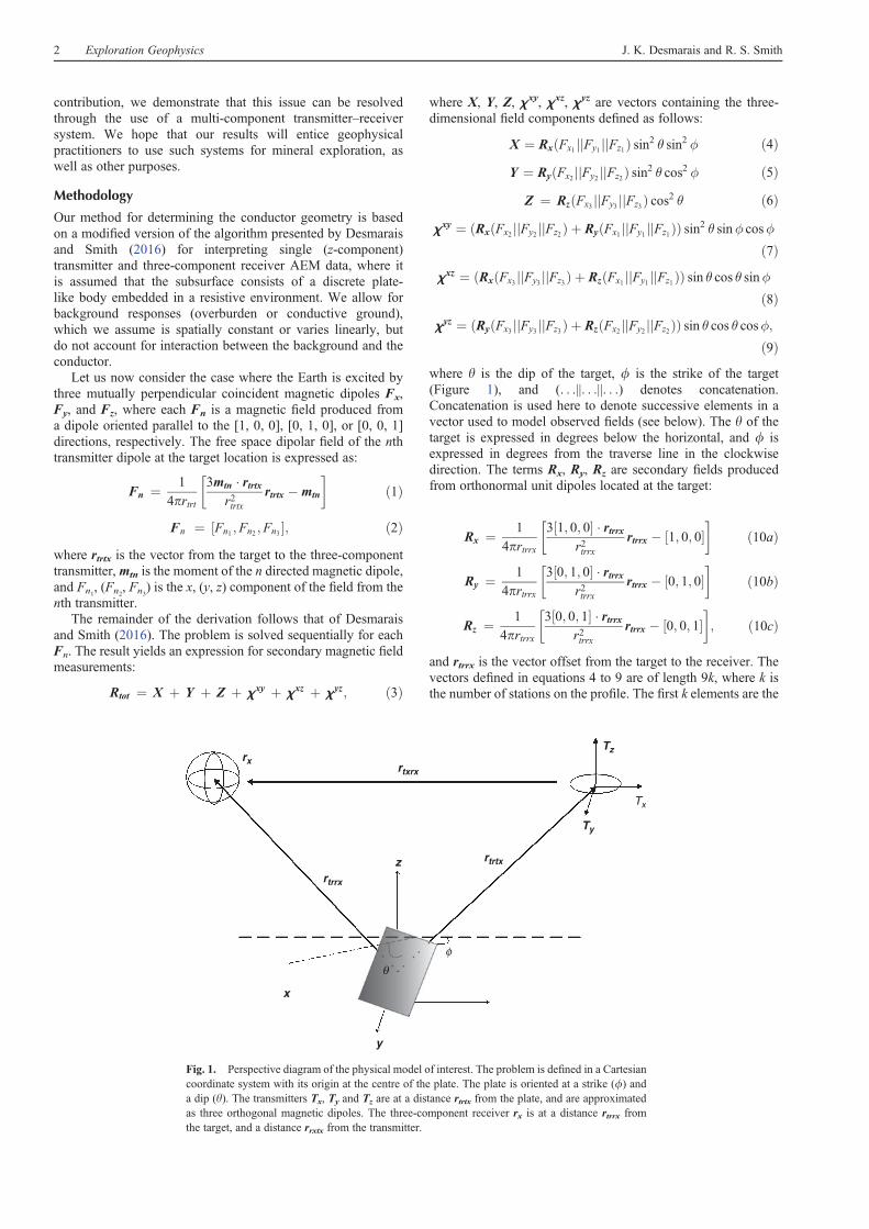
Fig. 1. Perspective diagram of the physical model of interest. The problem is defined in a Cartesiancoordinate system with its origin at the centre of the plate. The plate is oriented at a strike (f) anda dip (y). The transmitters Tx, Ty and Tz are at a distance rtrtx from the plate, and are approximatedas three orthogonal magnetic dipoles. The three-component receiver rx is at a distance rtrrx fromthe target, and a distance rrxtx from the transmitter.

2 Exploration Geophysics J. K. Desmarais and R. S. Smith

x-component response associated with the x-componenttransmitter, followed by k elements of the y-componentresponse for the x-component transmitter; then k elements forthe z-component response associated with the x-componenttransmitter; this pattern is repeated for the y-componenttransmitter and then the z-component transmitter. Thesevectors are a measure of how well the transmitter and receivercouple to the dipole in the ground with y and f. Equations 3–10are analogous to equations 15–16 in Desmarais and Smith(2016), except that the terms Fxm Fym Fzm, {m2 (1, 3)} inequations 4–9 of this paper, are replaced by Fx, y, z in equation16 of Desmarais and Smith (2016).

To model a vector of 9k observed AEM measurements RR,equation 3 is reformulated as follows:

RR ¼ aX þ bY þ gZ þ dxxy þ exxz þ zxyz

þX3

n¼ 1

ðlxnCxn þ lynCyn þ lznCzn þ mxnLxn

þ mynLyn þ mznLznÞ

ð11Þ

where a, b, g, d, e, z, lxn, mxn, lyn, myn, lzn, mxn are weightingcoefficients to be determined; Cxn, Cyn and Czn account forconstant backgrounds in the x-, y-, and z-components of themeasurements arising from coupling with the n-directedtransmitter dipole; and Lxn, Lyn, and Lzn account for linearbackgrounds in the x-, y-, and z-components of themeasurements arising from coupling with the n-directeddipole. A discussion on the need to account for both local andregional background effects can be found in Desmarais andSmith (2016). In the formulation of Desmarais and Smith(2016), for single-component transmitter, the vectors had alength 3k instead of 9k for a k station survey. The backgroundvectors contain zeroes, except for the elements associated withthe relevant component. For example, the Cy1 term associatedwith the x-component transmitter and the y-component receiverwill have a value of 1 in elements k+1 to 2k, whileLz3will containvalues varying linearly from –1 to 1 in elements 8k+1 to 9k.

The set of weighting coefficients are determined by solvinga linear system similar to the one presented in Desmarais andSmith (2016), except that the system is 24 dimensional insteadof 12 dimensional as a result of the 12 additional backgroundterms. The linear system is solved in a least-squares sensefor a particular set of system parameters {y, f, rtrtx, rtrrx} ona preselected profile of k points. The solution yields a set ofweighting coefficients that enable the estimation of backgroundfrom the field data.

In order to find the set of system parameters that best describethe measured data, we use a look-up table procedure. The systemparameters are sequentially varied, and the linear system issolved at each iteration. This yields an ensemble of weightingcoefficients over a region of parameter space. The ensemble ofweighting coefficients are used to build an ensemble of predictedresponses. The predicted responses are compared with themeasured response. The predicted response closest to themeasured response (having the highest index of fit) isassociated with a set of parameters {yp, fp, rtrtx

p , rtrrxp }, and

these parameters are the ones which best describe the dipolethat explains the measured data.

Results

Tests on synthetic models

In this section, we demonstrate that one of the benefits of usinga three-component transmitter system is that it is more robust

than a single-component transmitter for the estimation ofgeometrical parameters of a conductor. Single z-componenttransmitter systems frequently have difficulty resolving all theparameters of a conductor because the y-component is corruptedby noise due to overburden.Desmarais andSmith (2016) show anexample of a conductor at the Reid Mahaffy test site that doesnot have a clear y-component response because the backgroundnoise is high. Using a z-component transmitter system with noy-component receiver yields ambiguous answers. However, athree-component transmitter with no y-component receiver isable to resolve the geometrical parameters of the conductor. Infact, we show that measuring Rzx, Rzz with Ryx (where the firstletter denotes the orientation of the transmitter and the secondletter denotes the orientation of the receiver) is all that is neededto determine the geometrical parameters for the case of aMEGATEM system geometry.

Conductors produce small y-component anomalies when theyapproach symmetry with respect to the traverse line (Smith andKeating, 1996). For a plate-like conductor, symmetry equates tobeing at a small offset and having a f nearly perpendicular orparallel to the traverse line. If a plate is oriented parallel orperpendicular and at a small offset to the traverse line, thenfrom the point of view of an observer standing on the traverseline, the plate appears identical to the left and right of the observerand is therefore symmetric. Conductors responsible for AEManomalies can often be considered to effectively be at smalloffsets to the traverse line, since AEM responses are dominatedby material in the conductor that is close to the receiver.

How symmetric the conductor needs to be, in order to lack a y-component response, depends on the type of background. If thebackground generates a response larger than the y-componentresponse of an anomalous target, the target will produce asignificant anomaly in the x- and z-components but not the y-component. The lack of a y-component response increases theamount of zeroes in the matrix being inverted, correspondinglyincreasing its conditioning number. Therefore, if a conductordoes not produce a significant y-component anomaly, it isadvantageous to exclude this component from theinterpretation procedure. This can be accomplished by

180 1.0

0.9

0.8

0.7

0.6

0.5

0.4

0.3

0.2

0.1

0

160

140

120

100

80

60

40

20

00 10 20 30 40 50 60 70 80 90

( )

Str

ike

(deg

rees

from

trav

erse

line

)φ

( ) Dip (degrees from horizontal)θ

Strike and dip: y-component excludedφp,

I

(uni

tless

)θ,

φ

θ p

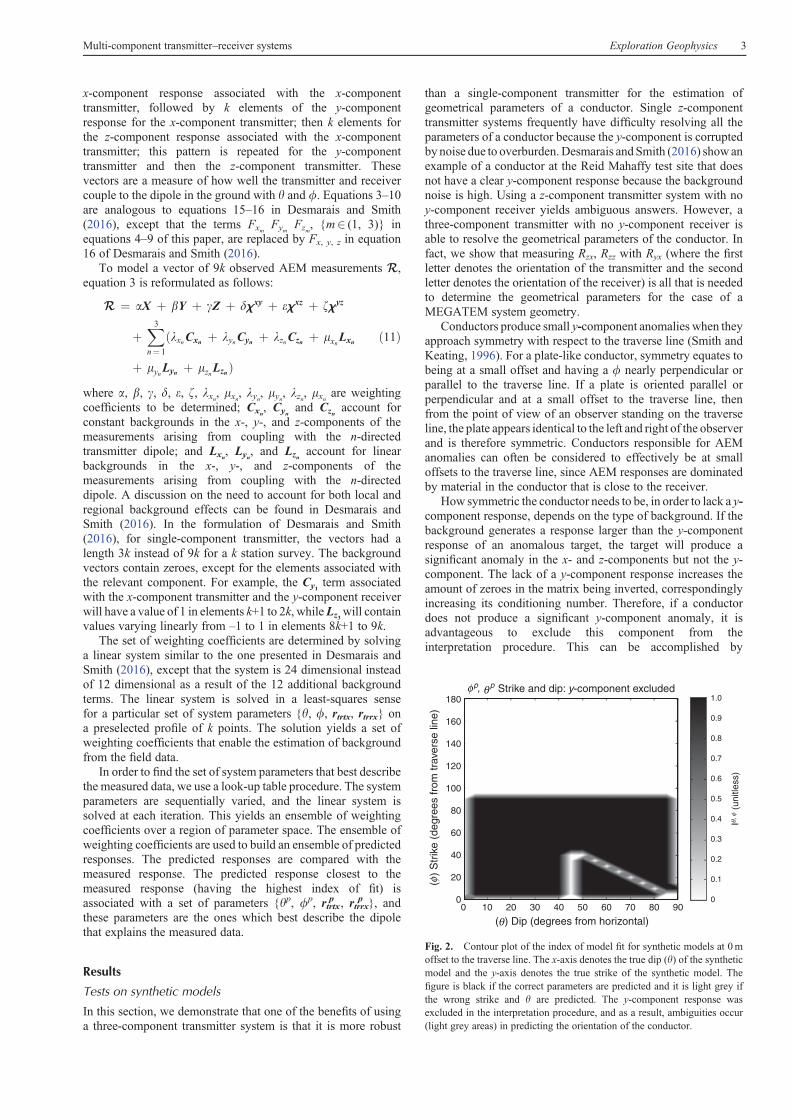
Fig. 2. Contour plot of the index of model fit for synthetic models at 0moffset to the traverse line. The x-axis denotes the true dip (y) of the syntheticmodel and the y-axis denotes the true strike of the synthetic model. Thefigure is black if the correct parameters are predicted and it is light grey ifthe wrong strike and y are predicted. The y-component response wasexcluded in the interpretation procedure, and as a result, ambiguities occur(light grey areas) in predicting the orientation of the conductor.

Multi-component transmitter–receiver systems Exploration Geophysics 3

8 (a)

(b)

(c)

x-component: = 70°, = 20°

y-component: = 70°, = 20°

z-component: = 70°, = 20°

×10–11

×10–10

×10–11

×10–10

×10–11

×10–10

6420

0

1

4

2

0

5

0

Res

pons

e (I

)R

espo

nse

(I)

Res

pons

e (I

)

–5

–10

–2

4

1

0

2

0

–2

–1

1

0

–1

1

0

–1

1

0

–1

–2–4

86420

–2–4–1500 –1000 –500 0 500 1000 1500

–1500 –1000 –500 0 500 1000 1500

–1500 –1000 –500 0

Profile position (m)



500 1000 1500

–1

–2

θ φ

θ φ

θ φ

x-component: = 45°, = 70°θ φ

y-component: = 45°, = 70°θ φ

z-component: = 45°, = 70°θ φ





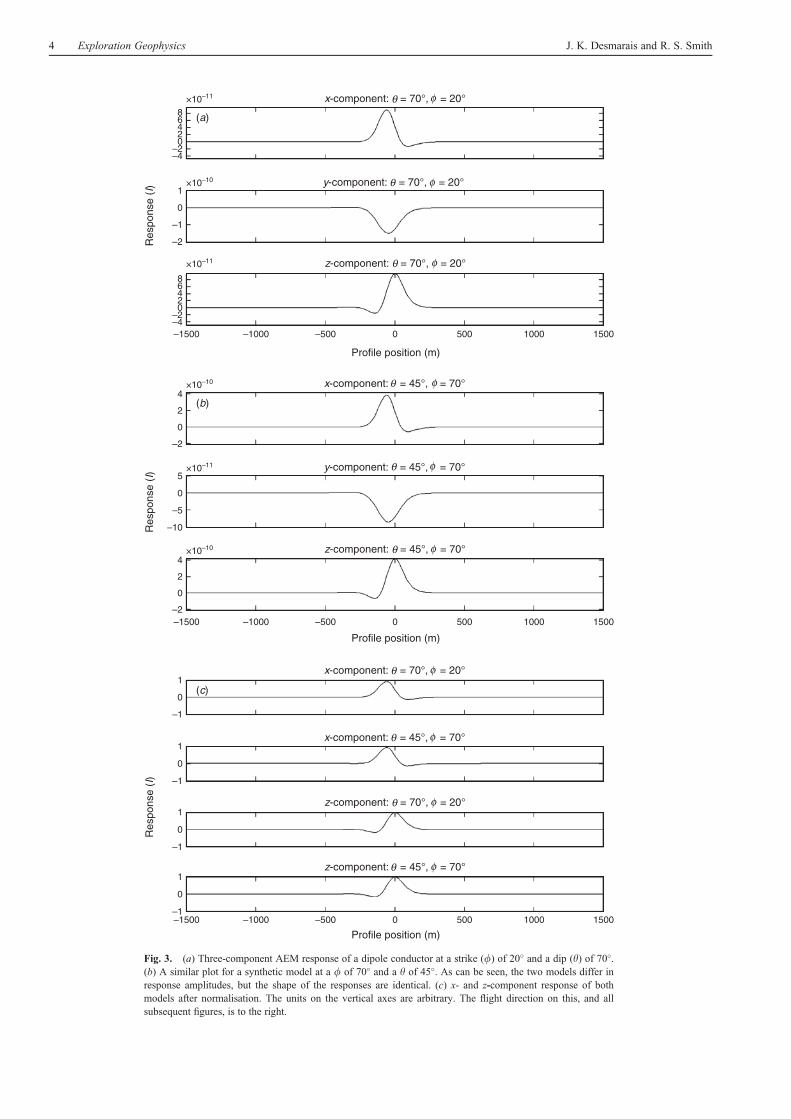
Fig. 3. (a) Three-component AEM response of a dipole conductor at a strike (f) of 20� and a dip (y) of 70�.(b) A similar plot for a synthetic model at a f of 70� and a y of 45�. As can be seen, the two models differ inresponse amplitudes, but the shape of the responses are identical. (c) x- and z-component response of bothmodels after normalisation. The units on the vertical axes are arbitrary. The flight direction on this, and allsubsequent figures, is to the right.


removing thebackground termsassociatedwith the y-component,and making all background and dipole vectors length 6k insteadof 9k for a k station survey.

To generate the synthetic models, the AEM system comprisesa multi-component transmitter flying along the x direction, andtowing a multi-component receiver offset by 128m in the x

4

2

1

4

2

0

–2

4

2

2

4

2

1

0

–1

1

0

–1

1

0

–1

1

0

–1

0

–2

1

0

0

–2

–1

0

0

–2

–2

–1

×10–10

×10–10

×10–10

×10–10

×10–10

×10–10

–1500 –1000 –500 0 500 1000 1500

–1500 –1000 –500 0 500 1000 1500

–1500 –1000 –500 0 500 1000 1500




Res

pons

e (I

)R

espo

nse

(I)

Res

pons

e (I

)(a)

(b)

(c)











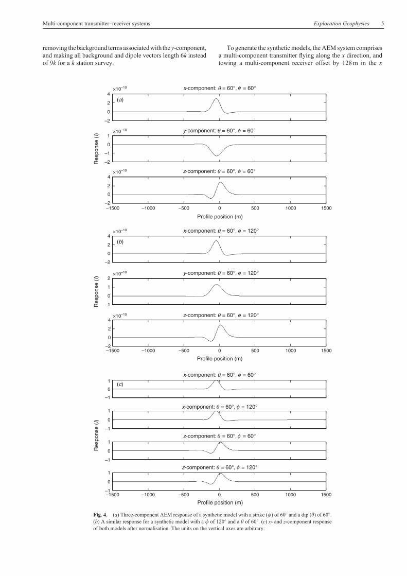
Fig. 4. (a) Three-component AEM response of a synthetic model with a strike (f) of 60� and a dip (y) of 60�.(b) A similar response for a synthetic model with a f of 120� and a y of 60�. (c) x- and z-component responseof both models after normalisation. The units on the vertical axes are arbitrary.


direction and 50m (down) in the z direction (the MEGATEMconfiguration). The dipolar target’s centre is positioned at 100mdepth in the centre of the profile (x= 0) at an offset of 0m to thetraverse line (y= 0).

The response from synthetic models were generated usingequation 3. A total of 703 models were tested with variable fand y. The f and y were varied at 5� intervals over the entirerange of target orientations {y2 (0, 90), f2 (0, 180)}. The yand f of the synthetic models was determined using the look-uptable approach described above and in Desmarais and Smith(2016). To image the estimated parameters, we use an index ofmodel fit similar to the one described in Desmarais and Smith(2016).

Figure 2 is a contour plot of the index of model fit for a setof synthetic models generated using a single-component (z-directed) transmitter and a two-component (x- and z-directed)receiver. Where the figure is dark, the index of model fit is closeto one and the correct f and y have been predicted. Where thefigure is light grey, the index of model fit is close to zero and theincorrect f and y have been predicted. Since Figure 2 is notcompletely dark, the index of model fit is not always in unity, andambiguities occur in predicting the orientation of the target.The light grey vertical feature occurring for synthetic modelsassociated with horizontal dips (y = 0�) occurs because when they is horizontal, the target couples with perfectly vertical fieldsregardless of thef. All of the horizontal (y= 0�) models thereforegenerate identical responses, and the f is unresolved.

Figure 2 also displays a light grey diagonal feature and a lightgrey vertical feature. The vertical feature occurswhen the y is 45�.An understanding of why these features emerge can be gatheredfrom Figure 3. The three-component response computed usingequation 3 for a synthetic model at a strike (f= 20�) and a dip(y = 70�) is shown in Figure 3a, while Figure 3b shows a similarresponse for a synthetic model at a strike of (f= 70�) and a dip(y = 45�). Comparing Figure 3a and Figure 3b, it is evident thatthe two models differ in absolute amplitudes, but the responseshapes and relative amplitudes of the components are identical.However, when implementing the interpretation algorithm ofDesmarais and Smith (2016), the amplitudes of the responses arenormalised. Normalisation is necessary to eliminate the effect ofdiffering delay time, conductivity, and body dimensions betweenthe observed data and the data in the look-up table. Modelprofiles are scaled through normalisation in order to have thesame maximum amplitude as that within the data segment underanalysis. This scaling is applied uniformly to all componentsused, so that x- and z-components (and y when used) have thesame scaling.

There is also a light grey horizontal feature associated withthe casewhen thef is parallel to the flight line (f = 0�), Figure 2).This occurs because, as the y varies, the shape and relativeamplitude of the x- and z-components remain constant, as inthe previous case. Therefore an ambiguity exists when predictingthe y of the conductor.

Figure 2 is grey for the models characterised by a strike(f > 90�). An understanding of why this occurs can begathered from Figure 4. Figure 4a shows a response associatedwith a synthetic model at a strike (f= 60�) and a dip(f= 60�).Figure 4b shows a similar response for a synthetic model with ay of 120� and a y of 60�. Comparing Figure 4a with Figure 4b, itcan be seen that these two models only differ in the sign ofthe y-component. Figure 4c shows the x- and z-componentresponses for the two models once they have been normalised.As before, the responses for both models are identical. A greyfeature also occurs for models having vertical dips y90�. Thisoccurs because, as the f changes from 90�, the amplitude of the

x- and z-components increases; however, their relativeamplitudes remain the same, so that the f is unresolved afternormalisation.

The problems outlined above do not persist for syntheticmodels at a non-zero offset to the traverse line, as theconductor is no longer symmetric, so that each value of f andy we tested generated x- and z-component responses that wereunique. However, this discussion is not concernedwithmodels atoffsets to the traverse line, since models at offsets to the traverseline generate y-component responses, and we are concerned withthe case where y-component data is too small or corrupted bynoise.

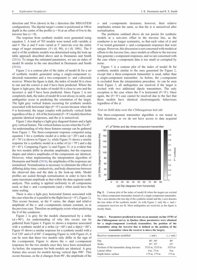
Figure 5 is a contour plot of the index of model fit forsynthetic models similar to the ones generated for Figure 2,except that a three-component transmitter is used, rather thana single-component transmitter. As before, the y-componentis excluded from the interpretation procedure. As can be seenfrom Figure 5, all ambiguities are resolved if the target isexcited with two additional dipole transmitters. The onlyexception is the case where the y is horizontal (y= 0�). Onceagain, the (y= 0�) case cannot be resolved due to the fact thatthese models have identical electromagnetic behavioursregardless of the f.

Test on field data over the Chibougamau test site

The three-component transmitter algorithm is not tested infield situations, as we do not have access to data acquired

180

160

140

120

100

80

60

40

20

00 10 20 30 40 50 60 70 80 90


( )

Str

ike

(deg

rees

from

trav

erse

line

)φ

1.0

0.9

0.8

0.7

0.6

0.5

0.4

0.3

0.2

0.1

0

Strike and dip: three-component transmitterφp, θ p

I

(uni

tless

)θ,

φ

Fig. 5. Contour plot of the index of model fit when the targets are excitedby a three-component transmitter instead of a single-component transmitter.The x-axis denotes the true dip of the synthetic model and the y-axis denotesthe true strike of the synthetic model. As with Figure 2, only the x- and z-component receivers are fit. Most ambiguities are resolved, as the figure ismostly black.

Table 1. Parameters predicted in tests on an anomaly on line 15701 ofthe Chibougamau survey in Quebec (these parameters were obtainedfor a single-component (vertical) transmitter; the position of thetransmitter along the traverse line is defined as the position of the

transmitter when the receiver is above the target).

Receiver components modelled x and z x, y and z

Dip 80�, 80� 80�

Strike 85�, 95� 65�

Position of the transmitter along traverse 5535m, 5535m 5555mLateral offset 0m, 75m 0mDepth below surface 175m, 175m 175m


using such an instrument. However, in what follows, wedisplay the failure of the single-component (vertical)transmitter algorithm to predict the orientation of theconductor when no y-component data is available. We hopethat this example will motivate the future use of multi-component transmitters.

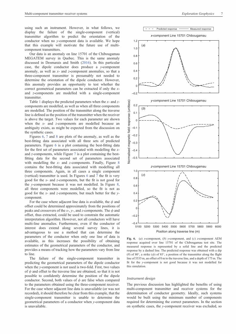
Our data is an anomaly on line 15701 of the ChibougamauMEGATEM survey in Quebec. This is the same anomalydiscussed in Desmarais and Smith (2016). In this particularcase, the dipole conductor does produce a y-componentanomaly, as well as x- and z-component anomalies, so that athree-component transmitter is presumably not needed todetermine the orientation of the dipole conductor. However,this anomaly provides an opportunity to test whether thecorrect geometrical parameters can be extracted if only the x-and z-components are modelled with a single-componenttransmitter.

Table 1 displays the predicted parameters when the x- and z-components are modelled, as well as when all three componentsare modelled. The position of the transmitter along the traverseline is defined as the position of the transmitter when the receiveris above the target. Two values for each parameter are shownwhen the x- and z-components are modelled because anambiguity exists, as might be expected from the discussion onthe synthetic cases.

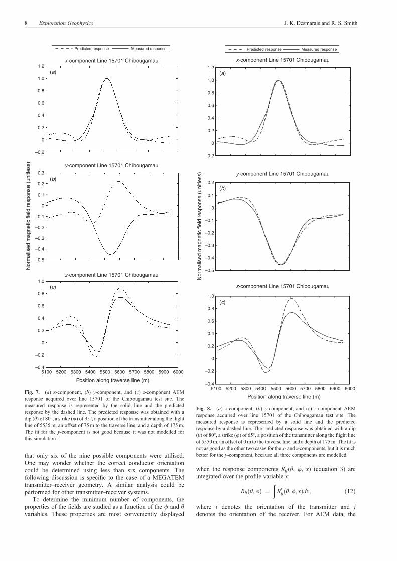
Figures 6, 7 and 8 are plots of the anomaly, as well as thebest-fitting data associated with all three sets of predictedparameters. Figure 6 is a plot containing the best-fitting datafor the first set of parameters associated with modelling the x-and z-components, while Figure 7 is a plot containing the best-fitting data for the second set of parameters associatedwith modelling the x- and z-components. Finally, Figure 8contains the best-fitting data associated with modelling allthree components. Again, in all cases a single component(vertical) transmitter is used. In Figures 6 and 7 the fit is verygood for the x- and z-components, but the fit is not good forthe y-component because it was not modelled. In Figure 8,all three components were modelled, so the fit is not asgood for the x- and z-components, but much better for the y-component.

For the case where adjacent line data is available, the f andoffset could be determined approximately from the positions ofpeaks and crossovers of the x-, y-, and z-components. The f andoffset, thus extracted, could be used to constrain the automaticinterpretation algorithm. However, not all conductors will havemulti-line anomalies. Furthermore, even if the conductor ofinterest does extend along several survey lines, it isadvantageous to use a method that can determine theparameters of the conductor when only one line of data isavailable, as this increases the possibility of obtainingestimates of the geometrical parameters of the conductor, andprovides a means of tracking how the parameters vary from lineto line.

The failure of the single-component transmitter inpredicting the geometrical parameters of the dipole conductorwhen the y-component is not used is two-fold. First, two valuesof f and offset to the traverse line are obtained, so that it is notpossible to confidently determine the position of the dipoleconductor. Second, both values of f are false when comparedto the parameters obtained using the three-component receiver.For the case where adjacent line data is unavailable (or was notrecorded), it should therefore be clear from this example, that thesingle-component transmitter is unable to determine thegeometrical parameters of a conductor when y-component datais unavailable.

Instrument design

The previous discussion has highlighted the benefits of usingmulti-component transmitter and receiver systems for thedetermination of conductor geometry. Ideally, such systemswould be built using the minimum number of componentsrequired for determining the correct parameters. In the sectionon synthetic cases, the y-component receiver was excluded, so

1.2

(a)

(b)

(c)

1.0

0.8

0.6

0.4

0.2

0

–0.2

0.2

0.1

0

–0.1

–0.2

–0.3

–0.4

–0.5

0.8

1.0

0.6

0.4

0.2

0

–0.2

–0.45100 5200 5300 5400

Position along traverse line (m)

Nor

mal

ised

mag

netic

fiel

d re

spon

se (

unitl

ess)

5500 5600 5700 5800 5900 6000

x-component Line 15701 Chibougamau

y-component Line 15701 Chibougamau

z-component Line 15701 Chibougamau

Predicted response Measured response

Fig. 6. (a) x-component, (b) y-component, and (c) z-component AEMresponse acquired over line 15701 of the Chibougamau test site. Themeasured response is represented by a solid line and the predictedresponse by a dashed line. The predicted response was obtained with a dip(y) of 80�, a strike (f) of 85�, a position of the transmitter along the flightline of 5535m, an offset of 0m to the traverse line, and a depth of 175m. Thefit for the y-component is not good because it was not modelled forthis simulation.


that only six of the nine possible components were utilised.One may wonder whether the correct conductor orientationcould be determined using less than six components. Thefollowing discussion is specific to the case of a MEGATEMtransmitter–receiver geometry. A similar analysis could beperformed for other transmitter–receiver systems.

To determine the minimum number of components, theproperties of the fields are studied as a function of the f and yvariables. These properties are most conveniently displayed

when the response components Rij0(y, f, x) (equation 3) are

integrated over the profile variable x:

Rijð�; �Þ ¼ðR0ijð�; �; xÞdx; ð12Þ

where i denotes the orientation of the transmitter and jdenotes the orientation of the receiver. For AEM data, the

1.2


1.0

0.8

0.6

0.4

0.2

0.3

1.0

0.8

0.6

0.4

0.2

0

–0.2

–0.4

0.2

0.1

0

0

–0.2

–0.1

–0.2

–0.3

–0.4

–0.5

5100 5200 5300 5400


5500 5600 5700 5800 5900 6000




Nor

mal

ised

mag

netic

fiel

d re

spon

se (

unitl

ess)

(a)

(b)

(c)

Fig. 7. (a) x-component, (b) y-component, and (c) z-component AEMresponse acquired over line 15701 of the Chibougamau test site. Themeasured response is represented by the solid line and the predictedresponse by the dashed line. The predicted response was obtained with adip (y) of 80�, a strike (f) of 95�, a position of the transmitter along the flightline of 5535m, an offset of 75m to the traverse line, and a depth of 175m.The fit for the y-component is not good because it was not modelled forthis simulation.

1.2

1.0

0.8

0.6

0.4

0.2

0

–0.2

0.2

0.1

0

–0.1

–0.2

–0.3

–0.4

–0.5

1.0

0.8

0.6

0.4

0.2

0

–0.2

–0.4

Nor

mal

ised

mag

netic

fiel

d re

spon

se (

unitl

ess)

(a)

(b)

(c)





5100 5200 5300 5400


5500 5600 5700 5800 5900 6000

Fig. 8. (a) x-component, (b) y-component, and (c) z-component AEMresponse acquired over line 15701 of the Chibougamau test site. Themeasured response is represented by a solid line and the predictedresponse by a dashed line. The predicted response was obtained with a dip(y) of 80�, a strike (f) of 65�, a position of the transmitter along the flight lineof 5550m, an offset of 0m to the traverse line, and a depth of 175m. The fit isnot as good as the other two cases for the x- and z-components, but it is muchbetter for the y-component, because all three components are modelled.


profile Rij0along the x-axis rarely has positive and negative

parts that are equal and opposite, consequently cancelling eachother and giving an integral of zero value; hence Rij is a goodapproximation of the amplitude of the response as a function ofy and f.

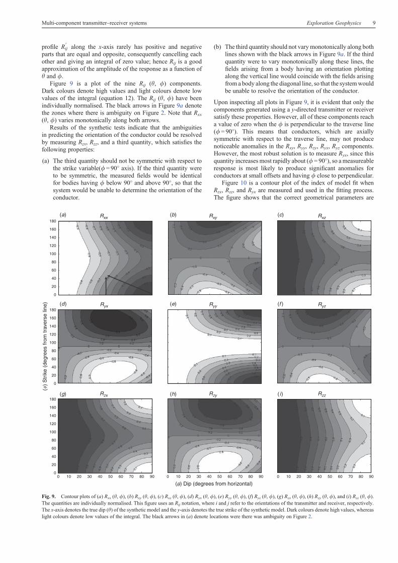
Figure 9 is a plot of the nine Rij (y, f) components.Dark colours denote high values and light colours denote lowvalues of the integral (equation 12). The Rij (y, f) have beenindividually normalised. The black arrows in Figure 9a denotethe zones where there is ambiguity on Figure 2. Note that Rxx

(y, f) varies monotonically along both arrows.Results of the synthetic tests indicate that the ambiguities

in predicting the orientation of the conductor could be resolvedby measuring Rzx, Rzz, and a third quantity, which satisfies thefollowing properties:

(a) The third quantity should not be symmetric with respect tothe strike variable(f= 90� axis). If the third quantity wereto be symmetric, the measured fields would be identicalfor bodies having f below 90� and above 90�, so that thesystem would be unable to determine the orientation of theconductor.

(b) The third quantity should not vary monotonically along bothlines shown with the black arrows in Figure 9a. If the thirdquantity were to vary monotonically along these lines, thefields arising from a body having an orientation plottingalong the vertical line would coincide with the fields arisingfrom a body along the diagonal line, so that the systemwouldbe unable to resolve the orientation of the conductor.

Upon inspecting all plots in Figure 9, it is evident that only thecomponents generated using a y-directed transmitter or receiversatisfy these properties. However, all of these components reacha value of zero when the f is perpendicular to the traverse line(f= 90�). This means that conductors, which are axiallysymmetric with respect to the traverse line, may not producenoticeable anomalies in the Rxy, Ryy, Rzy, Ryx, Ryz components.However, the most robust solution is to measure Ryx, since thisquantity increases most rapidly about (f= 90�), so a measureableresponse is most likely to produce significant anomalies forconductors at small offsets and having f close to perpendicular.

Figure 10 is a contour plot of the index of model fit whenRzx, Rzz, and Ryx are measured and used in the fitting process.The figure shows that the correct geometrical parameters are

180Rxx

Ryx

Rzx

Rxy

Ryy

Rzy

Rxz

Ryz

Rzz

160

140

120

100

80

60

40

20

0

180

160

140

120

100

80

60

40

20

0

180

160

140

120

100

80

60

40

20

00 10 20 30 40 50 60 70 80 90 0 10 20 30 40 50 60 70 80 90 0 10 20 30 40 50 60 70 80 90

( )

Str

ike

(deg

rees

from

trav

erse

line

)


(a) (b) (c)

(d) (e) (f )

(g) (h) ( i)

Fig. 9. Contour plots of (a) Rxx (y, f), (b) Rxy (y, f), (c) Rxz (y, f), (d) Ryx (y, f), (e) Ryy (y, f), (f) Ryz (y, f), (g) Rzx (y, f), (h) Rzy (y, f), and (i) Rzz (y, f).The quantities are individually normalised. This figure uses an Rij notation, where i and j refer to the orientations of the transmitter and receiver, respectively.The x-axis denotes the true dip (y) of the synthetic model and the y-axis denotes the true strike of the synthetic model. Dark colours denote high values, whereaslight colours denote low values of the integral. The black arrows in (a) denote locations were there was ambiguity on Figure 2.


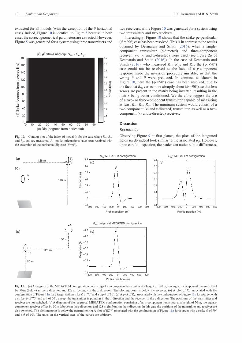
extracted for all models (with the exception of the y horizontalcase). Indeed, Figure 10 is identical to Figure 5 because in bothcases the correct geometrical parameters are extracted. However,Figure 5 was generated for a system using three transmitters and

two receivers, while Figure 10 was generated for a system usingtwo transmitters and two receivers.

Interestingly, Figure 10 shows that the strike perpendicular(f= 90�) case has been resolved. This is in contrast to the resultsobtained by Desmarais and Smith (2016), when a single-component transmitter (z-directed) and three-componentreceiver (x-, y-, and z-directed) were used (see figure 2a ofDesmarais and Smith (2016)). In the case of Desmarais andSmith (2016), who measured Rzx, Rzy, and Rzz, the (f > 90�)case could not be resolved as the lack of a y-componentresponse made the inversion procedure unstable, so that thewrong y and y were predicted. In contrast, as shown inFigure 10, here the (f= 90�) case has been resolved, due tothe fact that Ryx varies more abruptly about (f= 90�), so that lesszeroes are present in the matrix being inverted, resulting in thematrix being better conditioned. We therefore suggest the useof a two- or three-component transmitter capable of measuringat least Rzx, Rzz, Ryx. The minimum system would consist of atwo-component (y- and z-directed) transmitter, as well as a two-component (x- and z-directed) receiver.

Discussion

Reciprocity

Observing Figure 9 at first glance, the plots of the integratedfields Rij do indeed look similar to the associated Rji. However,upon careful inspection, the reader can notice subtle differences.

180

160

140

120

100

80

60

40

20

0

( )

Str

ike

(deg

rees

from

trav

erse

line

)φ

0 10 20 30 40 50 60 70 80 90

1.0

0.9

0.8

0.7

0.6

0.5

0.4

0.3

0.2

0.1

0


Strike and dip: Rzz, Rzx, Ryxφp, θ p

I

(uni

tless

)θ,

φ

Fig. 10. Contour plot of the index of model fit for the case where Rzz, Rzx

and Ryx and are measured. All model orientations have been resolved withthe exception of the horizontal dip case (y= 0�).

(a)128 m

128 m

1.2 0.6

0.5

0.4

0.3

0.2

0.1

0

–0.1

–1.2

–1.0

–0.8

–0.6

–0.4

–0.2

0.2

0

1.0

0.8

0.6

0.4

Res

pons

e (I

)R

espo

nse

(I)

0.2

–0.2–800 –600 –400 –200 0 200


400 600 800

0

120 m

50 m

70 m

50 m

rx

Tx

rz

Tz

(b)

(d) (e)

(c)

–800 –600 –400 –200 0 200

Rxz: reciprocal MEGATEM configuration

Rxz: MEGATEM configurationRzx: MEGATEM configuration

400 600 800

–800 –600 –400 –200 0 200



400 600 800

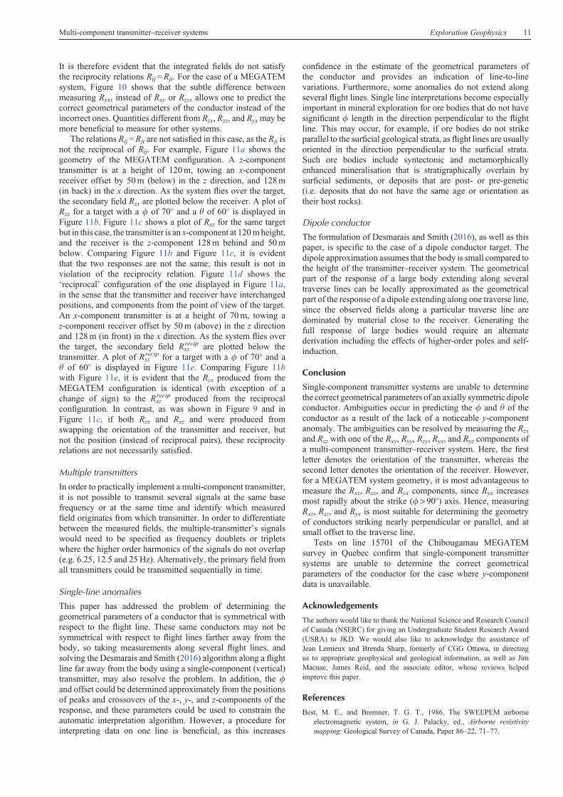
Fig. 11. (a) A diagram of the MEGATEM configuration consisting of a z-component transmitter at a height of 120m, towing an x-component receiver offsetby 50m (below) in the z direction and 128m (behind) in the x direction. The plotting point is below the receiver. (b) A plot of Rzx associated with theconfiguration of Figure 11a for a target with a strikef of 70� and a dip y of 60�. (c) A plot of Rxz associated with the configuration of Figure 11a for a target witha strike f of 70� and a y of 60�, except the transmitter is pointing in the x direction and the receiver in the z direction. The positions of the transmitter andreceiver are not switched. (d) A diagram of the reciprocal MEGATEM configuration consisting of an x-component transmitter at a height of 70m, towing a z-component receiver offset by 50m (above) in the z direction, and 128m (in front) in the x direction. In this case the positions of the transmitter and receiver arealso switched. The plotting point is below the transmitter. (e) A plot of Rxz

recip associated with the configuration of Figure 11d for a target with a strike f of 70�

and a y of 60�. The units on the vertical axes of the curves are arbitrary.


It is therefore evident that the integrated fields do not satisfythe reciprocity relations Rij =Rji. For the case of a MEGATEMsystem, Figure 10 shows that the subtle difference betweenmeasuring Ryx, instead of Rxy or Rzy, allows one to predict thecorrect geometrical parameters of the conductor instead of theincorrect ones. Quantities different from Rzx, Rzz, and Ryxmay bemore beneficial to measure for other systems.

The relations Rij =Rji are not satisfied in this case, as the Rji isnot the reciprocal of Rij. For example, Figure 11a shows thegeometry of the MEGATEM configuration. A z-componenttransmitter is at a height of 120m, towing an x-componentreceiver offset by 50m (below) in the z direction, and 128m(in back) in the x direction. As the system flies over the target,the secondary field Rzx are plotted below the receiver. A plot ofRzx for a target with a f of 70� and a y of 60� is displayed inFigure 11b. Figure 11c shows a plot of Rxz for the same targetbut in this case, the transmitter is an x-component at 120mheight,and the receiver is the z-component 128m behind and 50mbelow. Comparing Figure 11b and Figure 11c, it is evidentthat the two responses are not the same; this result is not inviolation of the reciprocity relation. Figure 11d shows the‘reciprocal’ configuration of the one displayed in Figure 11a,in the sense that the transmitter and receiver have interchangedpositions, and components from the point of view of the target.An x-component transmitter is at a height of 70m, towing az-component receiver offset by 50m (above) in the z directionand 128m (in front) in the x direction. As the system flies overthe target, the secondary field Rxz

recip are plotted below thetransmitter. A plot of Rxz

recip for a target with a f of 70� and ay of 60� is displayed in Figure 11e. Comparing Figure 11bwith Figure 11e, it is evident that the Rzx produced from theMEGATEM configuration is identical (with exception of achange of sign) to the Rxz

recip produced from the reciprocalconfiguration. In contrast, as was shown in Figure 9 and inFigure 11c, if both Rzx and Rxz and were produced fromswapping the orientation of the transmitter and receiver, butnot the position (instead of reciprocal pairs), these reciprocityrelations are not necessarily satisfied.

Multiple transmitters

In order to practically implement a multi-component transmitter,it is not possible to transmit several signals at the same basefrequency or at the same time and identify which measuredfield originates from which transmitter. In order to differentiatebetween the measured fields, the multiple-transmitter’s signalswould need to be specified as frequency doublets or tripletswhere the higher order harmonics of the signals do not overlap(e.g. 6.25, 12.5 and 25Hz). Alternatively, the primary field fromall transmitters could be transmitted sequentially in time.

Single-line anomalies

This paper has addressed the problem of determining thegeometrical parameters of a conductor that is symmetrical withrespect to the flight line. These same conductors may not besymmetrical with respect to flight lines farther away from thebody, so taking measurements along several flight lines, andsolving the Desmarais and Smith (2016) algorithm along a flightline far away from the body using a single-component (vertical)transmitter, may also resolve the problem. In addition, the fand offset could be determined approximately from the positionsof peaks and crossovers of the x-, y-, and z-components of theresponse, and these parameters could be used to constrain theautomatic interpretation algorithm. However, a procedure forinterpreting data on one line is beneficial, as this increases

confidence in the estimate of the geometrical parameters ofthe conductor and provides an indication of line-to-linevariations. Furthermore, some anomalies do not extend alongseveral flight lines. Single line interpretations become especiallyimportant in mineral exploration for ore bodies that do not havesignificant f length in the direction perpendicular to the flightline. This may occur, for example, if ore bodies do not strikeparallel to the surficial geological strata, as flight lines are usuallyoriented in the direction perpendicular to the surficial strata.Such ore bodies include syntectonic and metamorphicallyenhanced mineralisation that is stratigraphically overlain bysurficial sediments, or deposits that are post- or pre-genetic(i.e. deposits that do not have the same age or orientation astheir host rocks).

Dipole conductor

The formulation of Desmarais and Smith (2016), as well as thispaper, is specific to the case of a dipole conductor target. Thedipole approximation assumes that the body is small compared tothe height of the transmitter–receiver system. The geometricalpart of the response of a large body extending along severaltraverse lines can be locally approximated as the geometricalpart of the response of a dipole extending along one traverse line,since the observed fields along a particular traverse line aredominated by material close to the receiver. Generating thefull response of large bodies would require an alternatederivation including the effects of higher-order poles and self-induction.

Conclusion

Single-component transmitter systems are unable to determinethe correct geometrical parameters of an axially symmetric dipoleconductor. Ambiguities occur in predicting the f and y of theconductor as a result of the lack of a noticeable y-componentanomaly. The ambiguities can be resolved by measuring the Rzx

and Rzz with one of the Rxy, Ryy, Rzy, Ryx, and Ryz components ofa multi-component transmitter–receiver system. Here, the firstletter denotes the orientation of the transmitter, whereas thesecond letter denotes the orientation of the receiver. However,for a MEGATEM system geometry, it is most advantageous tomeasure the Rxz, Rzz, and Ryx components, since Ryx increasesmost rapidly about the strike (f > 90�) axis. Hence, measuringRxz, Rzz, and Ryx is most suitable for determining the geometryof conductors striking nearly perpendicular or parallel, and atsmall offset to the traverse line.

Tests on line 15701 of the Chibougamau MEGATEMsurvey in Quebec confirm that single-component transmittersystems are unable to determine the correct geometricalparameters of the conductor for the case where y-componentdata is unavailable.

Acknowledgements

The authors would like to thank the National Science and Research Councilof Canada (NSERC) for giving an Undergraduate Student Research Award(USRA) to JKD. We would also like to acknowledge the assistance ofJean Lemieux and Brenda Sharp, formerly of CGG Ottawa, in directingus to appropriate geophysical and geological information, as well as JimMacnae, James Reid, and the associate editor, whose reviews helpedimprove this paper.

References

Best, M. E., and Bremner, T. G. T., 1986, The SWEEPEM airborneelectromagnetic system, in G. J. Palacky, ed., Airborne resistivitymapping: Geological Survey of Canada, Paper 86–22, 71–77.


Davydycheva, S., 2010a, Separation of azimuthal effects for new-generationresistivity logging tools – Part I: Geophysics, 75, E31–E40. doi:10.1190/1.3269974

Davydycheva, S., 2010b, 3D modelling of new-generation (1999–2010)resistivity logging tools: The Leading Edge, 29, 780–789. doi:10.1190/1.3462778

Desmarais, J. K., and Smith, R. S., 2016, Decomposing the electromagneticresponse of magnetic dipoles to determine the geometric parametersof a dipole conductor: Exploration Geophysics, 47, 13–23. doi:10.1071/EG14070

Fraser, D. C., 1979, The multicoil II airborne electromagnetic system:Geophysics, 44, 1367–1394. doi:10.1190/1.1441013

Grant, F. S., and West, G. F., 1965, Interpretation theory in appliedgeophysics: McGraw-Hill.

Hogg, R. L. S., 1986, The AERODAT multigeometry, broadband transienthelicopter electromagnetic system, in G. J. Palacky, ed., Airborneresistivity mapping: Geological Survey of Canada, Paper 86–22, 79–89.

Raab, F. H., Blood, E. B., Steiner, T. O., and Jones, H. R., 1979, Magneticposition and orientation tracking system: IEEE Transactions onAerospace and Electronic Systems, AES-15, 709–718. doi:10.1109/TAES.1979.308860

Smith, R. S., 2014, Multi-component electromagnetic prospecting apparatusand method of use thereof: United States patent application publication.US Patent No. 2014/012505 A1.

Smith, R. S., and Keating, P. B., 1996, The usefulness of multicomponent,time-domain airborne electromagnetic measurements: Geophysics, 61,74–81. doi:10.1190/1.1443958

Smith, J. T., Morrison, H. F., Doolittle, L. R., and Tseng, H., 2007, Multi-transmitter multi-receiver null coupled systems for inductive detectionand characterization of metallic objects: Journal of Applied Geophysics,61, 227–234. doi:10.1016/j.jappgeo.2006.05.011

Snyder, D. D., and George, D. C., 2006, Qualitative and quantitative UXOdetection with EMI using arrays of multi-component receivers:Proceedings of the Symposium on the Application of Geophysics toEngineering and Environmental Problems, 19, 1749–1760.

Wang, G. L., Torres-Verdin, C., and Gianzero, S., 2009, Fast simulation oftriaxial borehole inductionmeasurements acquired in axially symmetricaland transversely isotropic media:Geophysics, 74, E233–E249. doi:10.1190/1.3261745

Wright, D. L., Moulton, C. W., Asch, T. H., Hutton, S. R., Brown, P. J.,Nabighian,M. N., and Li, Y., 2005, ALLTEM, a triangular wave on-timetime-domain system for UXO applications: Proceedings of theSymposium on the Application of Geophysics to Engineering andEnvironmental Problems, 18, 1357–1367.

Wright, D. L., Moulton, C. W., Asch, T. H., Brown, P. J., and Hutton, S. R.,2006, ALLTEM for UXO applications—first field tests: Proceedings ofthe Symposium on the Application of Geophysics to Engineering andEnvironmental Problems, 19, 1761–1775.

Wright,D.L.,Moulton,C.W.,Asch,T.H.,Brown,P. J.,Nabighian,M.N.,Li,Y., and Oden, C. P., 2007, ALLTEM UXO detection sensitivity andinversions for target parameters from Yuma proving ground test data:Proceedings of the Symposium on the Application of Geophysics toEngineering and Environmental Problems, 20, 1422–1435.


www.publish.csiro.au/journals/eg

dx.doi.org/10.1190/1.3269974

dx.doi.org/10.1190/1.3269974

dx.doi.org/10.1190/1.3462778

dx.doi.org/10.1190/1.3462778

dx.doi.org/10.1071/EG14070

dx.doi.org/10.1071/EG14070

dx.doi.org/10.1190/1.1441013

dx.doi.org/10.1109/TAES.1979.308860

dx.doi.org/10.1109/TAES.1979.308860

dx.doi.org/10.1190/1.1443958

dx.doi.org/10.1016/j.jappgeo.2006.05.011

dx.doi.org/10.1190/1.3261745

dx.doi.org/10.1190/1.3261745

Benefits of using multicomponent transmitter-receiver systems for determining geometrical parameters of a dipole conductor from single line anomalies

Documents