Bending of a Tapered Rod: Modern Application and ... · equilibrium is known for the deflection of a tapered rod. We report in this paper a comprehensive numerical analysis and experimental

World Journal of Mechanics, 2018, 8, 272-300 http://www.scirp.org/journal/wjm

ISSN Online: 2160-0503 ISSN Print: 2160-049X

DOI: 10.4236/wjm.2018.87022 Jul. 31, 2018 272 World Journal of Mechanics

Bending of a Tapered Rod: Modern Application and Experimental Test of Elastica Theory

M. P. Silverman, Joseph Farrah

Department of Physics, Trinity College, Hartford, USA

Abstract A tapered rod mounted at one end (base) and subject to a normal force at the other end (tip) is a fundamental structure of continuum mechanics that oc-curs widely at all size scales from radio towers to fishing rods to mi-cro-electromechanical sensors. Although the bending of a uniform rod is well studied and gives rise to mathematical shapes described by elliptic integrals, no exact closed form solution to the nonlinear differential equations of static equilibrium is known for the deflection of a tapered rod. We report in this paper a comprehensive numerical analysis and experimental test of the exact theory of bending deformation of a tapered rod. Given the rod geometry and elastic modulus, the theory yields virtually all the geometric and physical fea-tures that an analyst, experimenter, or instrument designer might want as a function of impressed load, such as the exact curve of deformation (termed the elastica), maximum tip displacement, maximum tip deflection angle, dis-tribution of curvature, and distribution of bending moment. Applied experi-mentally, the theory permits rapid estimation of the elastic modulus of a rod, which is not easily obtainable by other means. We have tested the theory by photographing the shapes of a set of flexible rods of different lengths and ta-pers subject to a range of impressed loads and using digital image analysis to extract the coordinates of the elastica curves. The extent of flexure in these experiments far exceeded the range of applicability of approximations that li-nearize the equations of equilibrium or neglect tapering of the rod. Agree-ment between the measured deflection curves and the exact theoretical pre-dictions was excellent in all but several cases. In these exceptional cases, the nature of the anomalies provided important information regarding the devia-tion of the rods from an ideal Euler-Bernoulli cantilever, which thereby per-mitted us to model the deformation of the rods more accurately.

Keywords Elastica, Deflection of Tapered Cantilever, Euler-Bernoulli Beam, Elastic

How to cite this paper: Silverman, M.P. and Farrah, J. (2018) Bending of a Tapered Rod: Modern Application and Experimental Test of Elastica Theory. World Journal of Mechanics, 8, 272-300. https://doi.org/10.4236/wjm.2018.87022 Received: June 19, 2018 Accepted: July 28, 2018 Published: July 31, 2018 Copyright © 2018 by authors and Scientific Research Publishing Inc. This work is licensed under the Creative Commons Attribution International License (CC BY 4.0). http://creativecommons.org/licenses/by/4.0/

Open Access

http://www.scirp.org/journal/wjm

https://doi.org/10.4236/wjm.2018.87022

http://www.scirp.org

https://doi.org/10.4236/wjm.2018.87022

http://creativecommons.org/licenses/by/4.0/

M. P. Silverman, J. Farrah

DOI: 10.4236/wjm.2018.87022 273 World Journal of Mechanics

Modulus, Flexure Formula

1. Introduction

Progress in physics is often made by creative application and testing of certain fundamental model systems relevant to new experimental methods and emerg-ing technologies. One such model system, which is the focal point of this paper, is the tapered cantilever, a structure whose shape under applied forces is of criti-cal interest to scientists and engineers in a wide range of fields of application. We report in this paper a comprehensive comparison of the theoretically pre-dicted and experimentally measured shapes of a flexible tapered rod described by this model system.

The theoretical shape of a flexible object bent by a load—historically referred to as the elastica—is an important part of the mechanics of continuous media. The basic equations relating the curvature of the shape and the bending moment of the object were first formulated by James Bernoulli in the late 17th Century and subsequently investigated in great detail by Euler in the mid 18th Century. In the years following Euler up to the present time, the theory of the elastica has been applied to numerous physical systems of great diversity ranging from large massive objects like bridges and architectural constructions, to medium size light-weight structures for aircraft and aerospace vehicles, to very small systems like the surface of a capillary or components of micro-electromechanical systems [MEMS]) [1] [2].

Among the fundamental model systems to which elastica theory pertains is that of a cantilever, a flexible structural element such as a rod or plate anchored at one end to a support. Physical examples of cantilevers, such as free-standing radio towers, brick chimneys, diving boards, mobile mechanical cranes, fixed-wing aircraft and many other systems, can be seen almost anywhere one looks. Much less visible and less widely known is the ubiquitous occurrence of cantilever structures in modern MEMS, such as cantilever transducers in atomic force microscopy [3], cantilever arrays in chemical sensors and biosensors for medical diagnostic applications [4].

A load applied to the free end of a cantilever is experienced at points throughout the length as a bending moment and shear stress. The proportional relationship between the curvature of the geometrical shape and the bending moment of the physical object defines the Euler-Bernoulli beam. Although there is an extensive pedagogical and research literature on the bending of structural elements modeled as cantilevers, most analyses, including those in advanced monographs such as [5] [6] [7], adopt the approximation, which in practice has come to characterize the Euler-Bernoulli beam, to neglect the square of the slope of the elastic curve in the equations of equilibrium. While this approximation may be valid in traditional engineering applications, the development of modern

https://doi.org/10.4236/wjm.2018.87022



composite materials, as well as the capacity to fabricate ultra-small, precisely shaped, compliant structures, have given rise to cantilever devices of great flex-ibility [8]. In such cases, the small-slope approximation, which reduces the ma-thematical analysis from a nonlinear to a linear equation, can lead to highly in-correct physical predictions.

Of the investigations of large deflections of cantilever beams known to the authors (see [9] [10] [11] and references therein), nearly all concerned beams of uniform cross section, since elastica theory in these cases can be solved in closed form in terms of incomplete elliptic integrals [12], as first done in [13]. Howev-er, many modern physical applications utilize tapered cantilever beams. Reasons for this configuration vary. In general, the bending moment of a cantilever is greatest at the support and diminishes to zero at the end. Thus, for macro-scale applications, there is no need to use as much material to maintain structural in-tegrity along the full length of the cantilever. Moreover, in certain specific mi-cro-scale applications, such as in atomic force microscopy and other mi-cro-electromechanical systems of importance in modern physics, the tapered de-sign is ideally suited to the function of the device.

To our knowledge, previous investigations of the deflection of tapered canti-levers employed various approximations to Euler-Bernoulli beams (see [14] [15] [16] [17] and references therein) with objectives very different from those of this paper. Nearly all were purely theoretical except for [14], which was concerned with the fracture of cantilever-shaped projectiles designed for ordnance. The earliest (and only) reference we know of a theoretical and experimental study of the large deflection of a tapered cantilever is [18], published in 1968, whereby the author tested predictions of just the end-point displacement as a function of applied force. Given the primitive state of computers at the time and the physical limitations of the available samples (wood, Plexiglas), no comparisons of calcu-lation and measurement comprising the full elastica shape of the test objects were given.

Benefiting from progress over the past half century of fast computers, ad-vanced symbolic mathematical software, sophisticated image analysis software, and strong, flexible synthetic materials, we report here what we believe to be the most comprehensive experimental and theoretical analysis of the elastica to date as it pertains to a tapered cantilever. In Section 2, the exact nonlinear differential equations for the equilibrium shape of an end-loaded tapered rod are derived, solved numerically, and compared with results for a uniform rod. In Section 3, the experimental procedure and analysis of a set of tapered rods of different lengths and taper ratios are described. Our conclusions are summarized in Section 4.

2. Equilibrium Shape of a Tapered Rod under Load

In this section we derive and solve the exact differential equations that deter-mine the equilibrium shape of a vertical tapered flexible rod with circular cross section subject to a constant horizontal force applied at the tip. The standard

https://doi.org/10.4236/wjm.2018.87022



assumptions for analysis of an ideal Euler-Bernoulli beam are made [19]; these include:

1) The length of the beam is much greater than the maximum cross-section radius;

2) The longitudinal axis of the beam lies within the neutral surface and does not experience a change of length under load;

3) The cross section of the beam at any location remains plane and perpendi-cular to the longitudinal axis during deflection;

4) Deformation of the cross section within its own plane is neglected; this is tantamount to neglect of bending-induced shear strain;

5) The normal stress within a cross section varies linearly with perpendicular distance from the neutral axis. In other words, the beam behaves like a linear elastic medium subject to Hooke’s law.

It is to be recalled that the neutral surface of a beam is the interface that sepa-rates the fibers under compression from the fibers under tension when the beam is bent by a load. The neutral axis within any cross section is the line of intersec-tion of the neutral surface with the cross section.

Figure 1 illustrates the system geometry pertinent to the analysis. The un-loaded, undeformed rod of length L is oriented vertically. Upon application of a horizontal force F applied at the tip, the rod, which is clamped at point O, bends as shown. Any point P along the curve of deformation (elastica curve) can be lo-cated by its longitudinal and transverse coordinates ( ),x y or by its arc length s and slope θ , i.e. the angle made by the tangent line at P to the vertical. The maximum longitudinal extension of the rod under load is of length a ; the angle of the tangent to the tip position where s L= is designated Lθ .

Figure 1. Deformation of a flexible rod of length L subject to a tip force F. The base is fixed at point O. An arbitrary point P on the curve of deformation (elastica) can be defined by coordi-nates x (longitudinal) and y (transverse) or by s (arc length) and θ (angle of tangent line).

https://doi.org/10.4236/wjm.2018.87022



The rod, itself, shown schematically in Figure 2, is a tapered circular cylinder with respective base and tip radii 0R , 1R , and apex angle given by

( ) ( )0 1tan 2 R R Lα = − . (1)

The radius of a circular cross section at an arbitrary arc length s follows from the geometry of similar triangles

( ) 10

0

1 1 Rsr s RL R

= + −

. (2)

Given the preceding assumptions, the theoretical relation that determines the shape of the bent rod is the Euler-Bernoulli flexure formula [20]

( ) ( ) ( )z zs M s EI sκ = (3)

relating the normal curvature ( )sκ [21],

( )

2 2

3 22

d d dd 1 d d

y xs y x

θκ = =

+

, (4)

to the product of the internal bending moment (torque) ( )zM s ,

( )dzS

M v v Sσ= −∫

, (5)

the bending moment of inertia ( )zI s computed about the neutral axis, 2dz

S

I v S= ∫∫ , (6)

and the modulus of elasticity (Young’s modulus) E. The integrals in Equation (5) and Equation (6) are over a cross-section ( )S s , v is the perpendicular distance from the neutral axis within a cross section, and ( )vσ

is the axial stress within the cross section. From the geometry shown in Figure 1 and Figure 2, it follows that the bending moment of the cantilever takes the form of a simple product

( ) ( )zM x F a x= − , (7)

and the bending moment of inertia is

( )4

10

0

1 1zRsI s I

L R

= + −

(8)

where

Figure 2. Geometry of the tapered rod: a truncated circular cylinder of length L with re-spective base and tip radii 0R , 1R . The radius r of an arbitrary cross section at arc length s is given by Equation (2) and the apex angle α is given by Equation (1).

https://doi.org/10.4236/wjm.2018.87022



40 0

π4

I R= (9)

is the bending moment of inertia of a uniform cylindrical rod of radius 0R .

2.1. Numerical Solution of the Exact Euler-Bernoulli Equation

The two equivalent expressions for curvature in Equation (4) suggest two possi-ble approaches to the equation of equilibrium, i.e. to find θ as a function of s, or y as a function of x. Although the function ( )y x provides the traditional and most convenient representation of the shape of the rod, a direct calculation of ( )y x would require solving the second-order nonlinear differential equa-tion

( )( )( )2 2

03 22

1

0

4d d 0

1 d d 1 1

F EI a xy x

Rsy xL R

−− =

+ − −

(10)

obtained by substituting Equations (7) and (8) into (3). Equation (10) poses at least two difficulties: 1) it contains both arc length s and longitudinal extension x, and the relation between s and x is not known in advance of the solution; 2) the maximum longitudinal extension a is also not known at the outset.

We seek instead a differential equation for θ as a function of s. Making the same substitutions into Equation (3) that led to Equation (10) now yields the first-order nonlinear differential equation

( )( )0

1

0

4d 0d

1 1

F EI a xs Rs

L R

θ −− = − −

(11)

which again contains x and a . However, upon taking the derivative of both sides of Equation (11) with respect to s and recognizing that

d d cosd d sinx sy s

θθ

==

(12)

one obtains after some algebra the second-order differential equation in norma-lized variables

( )( ) ( )

2

2 44 1d d cos 0

dd 1 1 1 1

Aρθ θ θσσ ρ σ ρ σ

−− + =

− − − − (13)

where A is a dimensionless rigidity constant 2

0A FL EI= , (14)

ρ is the ratio of tip to base radii

1 0R Rρ = , (15)

and

s Lx Ly L

σξη

===

(16)

https://doi.org/10.4236/wjm.2018.87022



are dimensionless variables that facilitate both the numerical computation and comparison of results for different rods and various values of tip load. The ad-vantage of Equation (13) is that it expresses the variation in θ with respect to only the variable σ ; the associated longitudinal variable ξ no longer appears.

As a second-order differential equation, Equation (13) requires two boundary conditions:

( )( )

1

0 0

d d 0.σ

θ

θ σ=

=

= (17)

The first condition applies because the rod is clamped at the base ( 0σ ξ= = ). The second condition applies because there is no bending moment at the tip ( 1σ = or a Lξ = ), as follows analytically from Equation (11).

Given its nonlinear character and complicated dependence on arc length, we know of no closed form analytical solution to Equation (13). To solve the equa-tion, therefore, we resorted to numerical methods implemented by Maple, which is one of the most powerful and widely used commercially available mathemati-cal engines. The Maple command dsolve, applied to an ordinary differential eq-uation (ODE) [in contrast to a partial differential equation (PDE)], utilizes one of several algorithms employing a trapezoidal method with Richardson en-hancement (also known as Richardson’s extrapolation to zero mesh width) [22] [23]. As an illustration of the numerical procedure, which may be helpful to readers who use a symbolic mathematical application, the command in our pro-gram took the form

([ ]

( ) )

: dsolve ode,numeric, range 0 1,

output ' listprocedure ',method bvp midrich ,

approxsoln :θ σ σ

Θ = =

= =

= =

(18)

which we interpret and explain as follows. The name ode is the expression symbolic of Equation (13). Use of normalized

variables (16) enabled us to confine the range of integration between 0 and 1, rather than a much larger range corresponding to the actual length L of a rod in physical units, which could impair convergence and greatly increase computa-tion time. The specific algorithm in statement (18) chosen for numerical solu-tion of the boundary value problem (bvp), termed midrich by Maple, is a mid-point method employing the Richardson extrapolation. The Maple default to-lerance limit is 10 digit precision, which is the level we employed. (One can change that level to n-digit precision by the global statement Digits: = n.) If the first two lines alone of command (18) are insufficient to achieve convergence, one could initiate the numerical method with the option approxsoln that sug-gests an approximate trial solution. In general, we found that a trial solution was needed only in cases of very large deformation, whereupon a simple linear ap-proximation ( )θ σ σ= worked satisfactorily.

The solution Θ returned by dsolve in (18) is a matrix function of the nor-malized arc length σ with components

https://doi.org/10.4236/wjm.2018.87022



( )1σ σΘ = (19)

( ) ( )2σ θ σΘ = (20)

( ) ( )3

dd

σ θ σσ

Θ = . (21)

To plot or compute with ( )θ σ , one must define a scalar function (designated in our program by the symbol ϑ ) by a statement such as

( )( ): ,evalϑ θ σ= Θ (22)

that creates a procedure, which in Maple is an object that can be invoked by a function, passed arguments, perform operations, and return results [24]. In Eq-uation (22) the procedure designated by ϑ evaluates the second component of Θ as a function of σ . Likewise, a statement such as

( )( )( ): , ,eval diffχ θ σ σ= Θ (23)

defines a scalar function χ that represents a procedure to evaluate the third component of Θ , which is the derivative ( )( ) ( ), d ddiff θ σ σ θ σ σ≡ , corres-ponding to the normalized curvature, Equation (4).

Examples of graphical solutions generated from command (18) are shown in Figure 3 and Figure 4. Figure 3 shows in Panel A the graphical output ( )θ σ vs σ for a rod characterized by 2 mL = , 0 1cmR = , 1 0.125 cmR = ,

6 GPaE = , and a sequence of loads ranging from 2 N to 10 N. As the load in-creases—i.e. plots range from a to e—the slope at the tip increases from about 70˚ to 90˚. Panel B shows the corresponding variation in curvature for the same sequence of increasing loads. With greater load, the flex point—point of greatest curvature—shifts to lower arc lengths, i.e. closer to the base of the rod.

Figure 4 provides a complementary perspective. Panel A shows ( )θ σ vs σ for a rod of the same length, base radius, and modulus as in the preceding figure, but for a fixed load of 10 N and a sequence of tip/base ratios ranging from 1:1 (plot a; no taper = uniform rod) to 1:16 (plot e; steep taper). For a fixed load, the

Figure 3. Tangent angle θ (Panel (A)) and associated curvature (Panel (B)) as a func-tion of normalized arc length σ for a rod of length 2 mL = , 0 1.0 cmR = ,

1 1 8 cmR = , modulus 6 GPaE = , and loads F (in N) of: (a) 2, (b) 4, (c) 6, (d) 8, (e) 10.

https://doi.org/10.4236/wjm.2018.87022



Figure 4. Tangent angle θ (Panel (A)) and associated curvature (Panel (B)) as a func-tion of normalized arc length σ for a rod of length 2 mL = , base radius 0 1.0 cmR = , modulus 6 GPaE = , load F = 10 N, and taper ratios of: (a) 1:1, (b) 1:2, (c) 1:4, (d) 1:8, (e) 1:16.

more tapered the rod, the greater is the deflection; at 10 N applied force, the tip angle of the rod with steepest taper was 90˚ compared with only 30˚ for the uni-form rod. Panel B again shows the corresponding variations in curvature. For a uniform rod (plot a) subject to fixed load, the curvature decreases linearly to 0 with arc length. With increasing taper, the curvature increases to higher maxi-mum values before plunging to 0 at the tip of the rod. The location of the maxi-mum curvature, however, is not very sensitive to the degree of taper. The total time taken by Maple to solve Equation (13) numerically and generate the five graphical solutions in each panel of the two figures did not exceed a few seconds.

From the numerical solution ( )θ σ , the corresponding elastica curve ( )η ξ was generated parametrically by integration of Equation (12) using what is termed an update equation [25]. Upon dividing the range [ ]0,1 of σ into N segments and defining the discrete tangent angle

( )k k Nθ θ≡ , (24)

for 0,1,2, ,k N= , the normalized Cartesian coordinates of the elastica can be calculated iteratively in steps of 1Nσ −∆ = by

( )( )

11

11

cos

sink k k

k k k

N

N

ξ ξ θ

η η θ

−−

−−

= +

= + (25)

from the initial conditions 0 0 0ξ η= = . Figure 5 and Figure 6 show the solu-tions ( )η ξ , corresponding respectively to the conditions of Figure 3 and Fig-ure 4, calculated from Equation (25) with N = 500. The time taken by Maple to generate the five elastica curves of each figure was again less than a few seconds. Figure 6 illustrates in a visually striking way that a highly tapered rod (plot e) can be bent nearly flat while the corresponding uniform rod subject to the same load suffers only a moderate deformation (plot a). In other words, neglect of ta-pering in the calculation of the deflection of a cantilever can lead to significant error.

https://doi.org/10.4236/wjm.2018.87022



Figure 5. Normalized horizontal deflection η as a function of normalized vertical ex-tension ξ for a rod corresponding to conditions of Figure 3.

Figure 6. Normalized horizontal deflection η as a function of normalized vertical ex-tension ξ for a rod corresponding to conditions of Figure 4.

2.2. Special Case I: Uniform Cross Section; Arbitrary Deflection

For a uniform rod the taper ratio 1 0 1R Rρ ≡ = , and therefore Equation (10) reduces to

( )( ) ( )3 222 2

0d d 1 d d 0y x F EI a x y x + − + = (26)

https://doi.org/10.4236/wjm.2018.87022



or, in terms of normalized variables,

( ) ( )3 222 2d d 1 d d 0LAη ξ α ξ η ξ + − + = , (27)

where

L a Lα = . (28)

Because the rod is rigidly fastened at the base, the boundary conditions of Equation (27) are

( )( )

0

0 0

d d 0ξ

η

η ξ=

=

= (29)

in contrast to the boundary conditions (17) of ( )θ σ , which constrain θ at the base and d dθ σ at the tip.

Although at first thought it may seem inconsistent that the Cartesian deriva-tive in (29) vanishes at the base whereas the angular derivative in (17) vanishes at the tip, there is no inconsistency. Recall that d dθ σ is proportional to the curvature κ , which is related to the second derivative of y with respect to x (or η with respect to ξ ), as given in Equation (4). Thus, setting ( )

0d d 0

xy x

==

in Equation (4) does not conflict with setting ( )d d 0x a

sθ== in Equation (11).

It is readily demonstrable, in fact, that both Equation (11) (or (13)) and Equa-tion (26) lead to the same value of curvature ( ) 00 Fa EIκ = at the base ( )0s x= = of the uniform rod. Starting with Equation (26), however, there is no a priori information by which to specify the value of d dy x at the tip ( ) or s L x a= = in advance of the solution.

Using the Maple command dsolve on Equation (27) yields an integral solution

( ) ( )2 20

2d

2 1 11 12 2

z z aA zAza Az Aza Az

ξ

η ξ−

= − + + −

∫ (30)

that can, with further effort, be cast into a complicated expression containing incomplete elliptic integrals. There is little point, however, in either making such a transformation or working with expression (30) because one can obtain com-putationally more useful relations by directly solving angular Equation (13), which reduces to

2

2

d cos 0d

Aθθ

σ+ = (31)

for 1ρ = . Equation (31) takes the form of Newton’s second law of motion for a particle

of unit mass subject to a force cosA θ− . Note, this is just an analogy with θ the analogue of particle coordinate and σ the analogue of time. Consider this problem from the perspective of Lagrangian and Hamiltonian mechanics [26]. The Lagrangian function ( ),L θ θ then takes the form

( ) 21, Kinetic Energy Potential Energy sin2

L Aθ θ θ θ= − = − (32)

https://doi.org/10.4236/wjm.2018.87022



where d dθ θ σ≡ . The canonical momentum p is defined by

p L θ θ= ∂ ∂ = (33)

from which the Hamiltonian follows by a Legendre transformation [27]

( ) ( ) 21, , sin2

H p p L p Aθ θ θ θ θ= − = + . (34)

It is straightforward to verify that the Hamiltonian equations of motion lead directly to Equations (31) and (33)

cos 0p H Aθ θ θ= −∂ ∂ ⇒ + =

(35)

H p pθ θ= ∂ ∂ ⇒ = . (36)

Substitution of p given by Equation (36) into the Hamiltonian (34) yields

21 sin2

H Aθ θ= + (37)

which must be a conserved quantity (i.e. a constant) since H is not an explicit function of σ .

The constant is found by evaluating Equation (37) at the end point of the rod for which ( )1 Lθ θ= (see Figure 1) and ( )1 0θ = . Thus one obtains the equiv-alent of a first integral of motion

21 sin sin2 LA Aθ θ θ+ = (38)

from which follows the derivative

( )d d 2 sin sinLAθ σ θ θ= − (39)

and by integration the coordinates of the elastica of a uniform rod in parametric form

( )0

1 d2 sin sinL

zA z

θ

σ θθ

=−∫ (40)

( )0

1 cos d2 sin sinL

z zA z

θ

ξ θθ

=−∫ (41)

( )0

1 sin d2 sin sinL

z zA z

θ

η θθ

=−∫ , (42)

where use has been made of Equation (12). While it is often advantageous to have closed-form solutions to a problem, it

should be noted that an alternative and computationally more efficient way to obtain the elastica coordinates ( ),ξ η from the derivative (39) is to apply again the iterative algorithm (25). It takes much more computer time to evaluate the elliptic integrals (41) and (42) than to process the update algorithm even for N on the order of 1000. Computation time is relevant here because the boundary value Lθ (i.e. tangent angle at the tip) is not known at the outset and must be determined by trial and error. One way to do this is by numerically finding the value of Lθ for which the integral (40) is unity

https://doi.org/10.4236/wjm.2018.87022



( )0

1 d12 sin sin

L

LL

L zL A z

θ

σ θθ

= = =−∫ . (43)

2.3. Special Case II: Uniform Cross Section; Small-Angle Approximation

For purposes of comparison we consider the familiar case of small-angle deflec-tion of a rod of uniform cross section. This is the case described by the Eu-ler-Bernoulli approximation which neglects ( )2d dy x in Equation (10), which thereby reduces to

( )2 2d d LAη ξ α ξ= − (44)

in normalized coordinates for 1ρ = . Equation (44) can be integrated directly to yield the third-order polynomial

( ) 21 12 3LAη ξ ξ α ξ = −

. (45)

The value of the maximum longitudinal extension, L a Lα = , is again not known at the outset and can be determined by requiring, as was done with Equ-ation (43), the full normalized length of the rod to be unity:

( ) ( )2

01 d d d 1L

Lα

σ α η ξ ξ= + =∫ . (46)

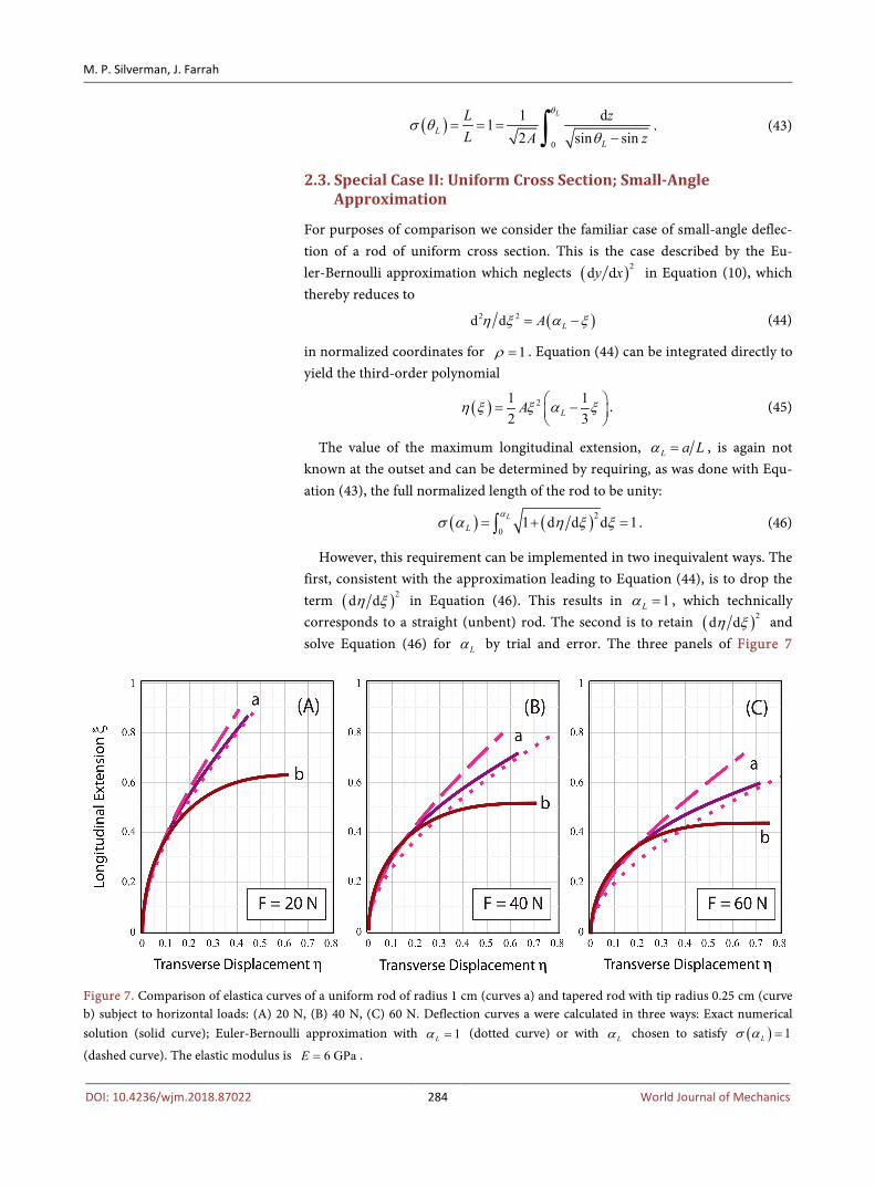
However, this requirement can be implemented in two inequivalent ways. The first, consistent with the approximation leading to Equation (44), is to drop the term ( )2d dη ξ in Equation (46). This results in 1Lα = , which technically corresponds to a straight (unbent) rod. The second is to retain ( )2d dη ξ and solve Equation (46) for Lα by trial and error. The three panels of Figure 7

Figure 7. Comparison of elastica curves of a uniform rod of radius 1 cm (curves a) and tapered rod with tip radius 0.25 cm (curve b) subject to horizontal loads: (A) 20 N, (B) 40 N, (C) 60 N. Deflection curves a were calculated in three ways: Exact numerical solution (solid curve); Euler-Bernoulli approximation with 1Lα = (dotted curve) or with Lα chosen to satisfy ( ) 1Lσ α =

(dashed curve). The elastic modulus is 6 GPaE = .

https://doi.org/10.4236/wjm.2018.87022



show comparative plots of the resulting elastica curves for a uniform rod (plots a) subject to what may be considered small, medium, and large loads. In all three cases one finds that • the first method ( 1Lα = ) leads to an approximate curve (dotted) that gener-

ally follows the exact curve (solid) but is in increasingly poor agreement over its entire length as the load and deformation increase;

• the second method ( ( ) 1Lσ α = ) leads to an approximate curve (dashed) that agrees well with the exact curve, even for large deformations, up to the point where the exact curve begins to flatten, after which the two curves diverge markedly.

Superposed on the plots in the three panels is the exact curve (plot b), calcu-lated from Equation (13) for a corresponding tapered rod with taper ratio 1:4. One sees again that for a given load the deflection of a tapered rod is much greater than that of a uniform rod.

3. Experimental Test and Determination of Elastic Modulus

An experimental configuration corresponding closely to that of Figure 1 was set up to record photographically and measure accurately the deformations pro-duced on a set of five fishing rods of different lengths and tapers. The geome-trical features of the rods are summarized in Table 1. In the US, fishing rod sizes and load-bearing capabilities are generally given in English units (feet; pounds); these are shown in the tables and associated figures of this paper, but analyses were implemented in metric units. The symbol W represents load in pounds, in contrast to F, which represents force in newtons.

A fishing rod is a cantilever of exceptional flexibility designed for casting an artificial lure made of lightweight materials. Modern fishing rods are a compo-site of synthetic materials such as fiberglass, carbon/graphite, Kevlar, boron, or some combination of these in a matrix of polyester or epoxy resin [28]. The fi-bers are laid down in a complex pattern designed to prevent the rod from flat-tening under stress. Apart from the handle of the rod, which is generally a non-flexible material covered with a frictional surface like cork to prevent slip-page, the cantilever portion usually has a fairly uniform taper. The degree of ta-per determines the extent of flexure for a given stress, as illustrated in Figure 6. Rods that deflect over a greater portion of their length are easier to cast and Table 1. Geometric properties of the rods.

Rod No. Total Length

(ft) Length without

Handle (m) Base Diameter

(cm) Tip Diameter

(cm)

1 6 1.52 1.2 0.3

2 6 1.52 1.0 0.3

3 7 1.68 1.3 0.3

4 7 1.52 1.6 0.3

5 10 2.44 1.7 0.3

https://doi.org/10.4236/wjm.2018.87022



present a wide forward loop of a kind that is often pictured in sports magazines and tourist literature devoted to outdoor activities.

Since fishing is a sport and hobby of immense popularity worldwide with a li-terature (dating back centuries) believed to be more abundant than that of any other individual sport [28], it is important to note that the analysis and experi-ment presented in this paper have practical ramifications beyond testing a fun-damental part of the mechanics of continuous media. First, the experimental procedure and theoretical analysis together provide a means of deducing the elastic modulus E of an individual fishing rod, which, given the complexity of the composition and construction of a rod, is difficult to measure in other ways. To judge from the numerous inquiries for E that we have seen on the internet, this is a material property of interest to prospective purchasers and users of fishing rods. However, we have been unable to find any values of E reported by rod manufacturers or vendors for their rods. At best, one can find broad ranges for different materials [29].

Second, rod manufacturers have tried various means of static deflection pro-filing [28] to correlate the deflection shape, tip deflection distance, and im-pressed weight for purposes of rod classification. In this regard an important practical outcome of this paper is to provide the means of predicting exactly the entire rod geometry under static deflection once the rod length, base and tip ra-dii, modulus, and load are given. Thus, provided the rod behaves like a linear elastic medium in keeping with the assumptions of Section 2, this paper removes all guesswork from establishing the correlations among impressed force, shape, and maximum deflection.

3.1. Procedure and Data

The deflection curve of each of the five rods in Table 1 was measured for each of four impressed horizontal loads in the following way. A rod was positioned ver-tically and fastened so that the handle of the rod was immobilized and only the tapered cantilever portion of the rod could deflect under stress. The stress was transmitted to the rod by means of a thin nylon fishing line attached at the tip of the rod and pulled horizontally at a force measured by an attached digital scale calibrated in pounds and accurate to 0.01 lb (0.0445 N). Positioned close to the rod was a vertical post with two points calibrated to be 1 0.002± m apart. At static equilibrium, a digital photograph was taken of the deflected rod and cali-bration post for processing by the image analysis software called Tracker [30].

Tracker is an open-source modeling tool created by Douglas Brown and available for Mac, Windows, and Linux platforms. Detailed operational informa-tion is available at the referenced web site, but, in brief, we obtained the coordi-nates of the rod deflection curves by • importing a digital photo of each rod subject to each load (5 rods × 4 loads)

into the application; • setting the origin of the Cartesian coordinate system with respect to which

the points on the deflection curve of a rod were to be measured;

https://doi.org/10.4236/wjm.2018.87022



• correlating the calibration length in the photo with a proxy calibration line in the computer display;

• selecting a representative sample of equally spaced points along the full length of the deflection curve with the computer mouse.

The Tracker output yielded the experimental coordinates ( ),x y = (longitu-dinal extension, transverse deflection) in units of our calibration length, which was taken to be 1 m. Each pair of coordinates was then divided by the length of the rod (not including the handle) to yield the normalized points ( ),ξ η . Tables 2-6 summarize the normalized coordinates deduced from Tracker for Rods 1, 2, Table 2. Deformation of Rod 1 as a function of load (L = 1.524 m).

Force (lbs) 2 4 6 8

Force (N) 8.896 17.793 26.689 35.586

Arc σ ξ η ξ η ξ η ξ η

0.000 0.000 0.000 0.000 0.000 0.000 0.000 0.000 0.000

0.100 0.006 0.084 0.013 0.084 0.019 0.084 0.019 0.084

0.200 0.019 0.162 0.039 0.149 0.045 0.149 0.052 0.143

0.300 0.058 0.253 0.084 0.227 0.104 0.221 0.117 0.208

0.400 0.104 0.325 0.149 0.286 0.175 0.273 0.195 0.247

0.500 0.169 0.383 0.234 0.338 0.253 0.318 0.286 0.279

0.600 0.247 0.442 0.312 0.357 0.344 0.338 0.370 0.286

0.700 0.331 0.481 0.422 0.370 0.442 0.344 0.474 0.292

0.800 0.429 0.494 0.494 0.377 0.539 0.351 0.565 0.292

0.900 0.519 0.500 0.597 0.377 0.623 0.351 0.656 0.292

1.000 0.604 0.506 0.669 0.377 0.708 0.351 0.734 0.292

Table 3. Deformation of Rod 2 as a function of load (L = 1.524 m).

Force (lbs) 2 4 6 8

Force (N) 8.896 17.793 26.689 35.586


0.000 0.000 0.000 0.000 0.000 0.000 0.000 0.000 0.000

0.100 0.007 0.092 0.013 0.099 0.013 0.086 0.020 0.086

0.200 0.020 0.178 0.033 0.171 0.039 0.164 0.046 0.164

0.300 0.046 0.257 0.072 0.257 0.092 0.250 0.105 0.243

0.400 0.086 0.349 0.132 0.336 0.151 0.309 0.171 0.303

0.500 0.145 0.434 0.197 0.401 0.230 0.368 0.257 0.355

0.600 0.197 0.507 0.270 0.461 0.316 0.408 0.336 0.388

0.700 0.276 0.572 0.355 0.500 0.408 0.434 0.434 0.408

0.800 0.362 0.618 0.447 0.520 0.500 0.441 0.526 0.414

0.900 0.467 0.638 0.539 0.533 0.599 0.441 0.625 0.414

1.000 0.546 0.651 0.638 0.533 0.691 0.441 0.717 0.414

https://doi.org/10.4236/wjm.2018.87022




Force (lbs) 2 4 6 8

Force (N) 8.896 17.793 26.689 35.586


0.000 0.000 0.000 0.000 0.000 0.000 0.000 0.000 0.000

0.091 0.006 0.083 0.006 0.083 0.012 0.083 0.012 0.083

0.182 0.012 0.173 0.024 0.167 0.024 0.167 0.030 0.167

0.273 0.018 0.256 0.042 0.250 0.048 0.250 0.060 0.250

0.364 0.036 0.333 0.065 0.333 0.083 0.333 0.095 0.327

0.455 0.054 0.417 0.095 0.405 0.125 0.399 0.143 0.393

0.546 0.083 0.506 0.143 0.488 0.179 0.470 0.202 0.458

0.637 0.119 0.583 0.202 0.548 0.244 0.524 0.274 0.506

0.727 0.167 0.661 0.274 0.607 0.321 0.560 0.351 0.542

0.818 0.220 0.726 0.345 0.643 0.405 0.589 0.435 0.560

0.909 0.292 0.780 0.435 0.667 0.488 0.589 0.518 0.565

1.000 0.363 0.821 0.512 0.667 0.565 0.589 0.595 0.565


Force (lbs) 2 4 6 8

Force (N) 8.896 17.793 26.689 35.586


0.000 0.000 0.000 0.000 0.000 0.000 0.000 0.000 0.000

0.100 0.007 0.092 0.007 0.092 0.007 0.092 0.007 0.092

0.200 0.013 0.184 0.013 0.184 0.020 0.191 0.020 0.191

0.300 0.013 0.289 0.026 0.289 0.033 0.289 0.046 0.289

0.400 0.026 0.382 0.046 0.382 0.059 0.382 0.079 0.375

0.500 0.046 0.480 0.066 0.474 0.099 0.474 0.125 0.461

0.600 0.072 0.572 0.112 0.559 0.151 0.546 0.184 0.526

0.700 0.118 0.658 0.178 0.632 0.224 0.599 0.263 0.579

0.800 0.191 0.717 0.257 0.671 0.316 0.625 0.349 0.592

0.900 0.283 0.750 0.362 0.684 0.414 0.625 0.447 0.592

1.000 0.382 0.763 0.454 0.684 0.513 0.625 0.546 0.592

3, 4, 5, respectively. The coordinates reported in Tables 2-6 comprise the expe-rimental points in the graphical comparisons of experiment and theory shown in Figures 8-12 and discussed in Section 3.2. It will be seen that the theory devel-oped in Section 2 accounted very well for the deflection curves of Rods 1-3 and the large-angle deflection curves of Rod 5. Anomalies observed for Rod 4 and the small-angle deflection curves of Rod 5 point to deviations from ideality with

https://doi.org/10.4236/wjm.2018.87022




Force (lbs) 2 4 6 8

Force (N) 8.896 17.793 26.689 35.586


0.000 0.000 0.000 0.000 0.000 0.000 0.000 0.000 0.000

0.063 0.004 0.061 0.004 0.061 0.008 0.061 0.008 0.061

0.125 0.008 0.123 0.012 0.123 0.016 0.123 0.016 0.123

0.188 0.012 0.184 0.020 0.184 0.029 0.180 0.033 0.180

0.250 0.016 0.246 0.029 0.246 0.041 0.229 0.049 0.229

0.313 0.029 0.303 0.045 0.299 0.061 0.287 0.070 0.287

0.375 0.037 0.361 0.061 0.356 0.086 0.340 0.098 0.336

0.438 0.049 0.422 0.082 0.410 0.115 0.397 0.131 0.389

0.500 0.061 0.479 0.107 0.467 0.148 0.447 0.164 0.438

0.563 0.078 0.541 0.135 0.525 0.188 0.500 0.209 0.484

0.625 0.098 0.594 0.168 0.570 0.225 0.537 0.254 0.520

0.688 0.127 0.656 0.209 0.623 0.279 0.582 0.307 0.557

0.750 0.156 0.705 0.250 0.664 0.328 0.606 0.356 0.582

0.813 0.193 0.754 0.303 0.705 0.385 0.635 0.418 0.598

0.875 0.229 0.799 0.348 0.733 0.443 0.643 0.471 0.611

0.938 0.262 0.828 0.397 0.750 0.492 0.652 0.520 0.615

1.000 0.311 0.861 0.443 0.766 0.541 0.652 0.570 0.615

respect to the Euler-Bernoulli beam.

3.2. Experimental Deflection Curves

A comparison of theoretical and experimental deflection curves for Rods 1 through 5 is shown graphically in Figures 8-12 respectively. Each figure com-prises four panels corresponding to each of the four impressed loads (W = 2, 4, 6, 8 pounds). Within each panel, the solid wine-colored curve is the theoretically predicted elastica curve obtained by solving Equation (13), given the known geometry of the rod, the load, and the initially unknown elastic modulus E. Val-ues for E were determined by trial and inspection of the resulting match with the experimental curve marked by blue solid-circle plotting symbols at points where the image-analysis software was instructed to determine coordinates. For pur-poses of comparison, the exact deflection curve of the corresponding uniform rod (dashed black curve) and the Euler-Bernoulli approximate deflection curve of correct total arc length (solid pink curve) are also shown in each panel.

In regard to our method of curve fitting and parameter estimation, it bears emphasizing for both conceptual and practical reasons that there was nothing to be gained by using a statistical fitting procedure, such as the method of maxi-mum likelihood or method of least-squares [31]. Indeed, use of such a fitting

https://doi.org/10.4236/wjm.2018.87022



Figure 8. Comparison of (a) exact elastica theory (heavy solid maroon line) and experimental deformations (blue circles) of Rod 1 for specified loads W in pounds. System parameters are: length 1.52 m, taper ratio 0.25, and mean modulus 6.0 0.4 GPaE ≈ ± . Superposed on each plot are the deformation curve for a uniform rod calculated (b) exactly (dashed black line) and (c) by linear approximation (thin solid pink line).

procedure would have been inappropriate for the problem at hand.

As a practical matter, the method of trial and inspection was implementable by computer very quickly and led to highly satisfactory, if not nearly perfect, fits of theory and experiment shown in Figures 8-10. A numerical value of E ade-quate to our purpose could be obtained by trial and inspection for each match of theory with experiment in just a few minutes. Use of a statistical fitting proce-dure on a nonlinear differential equation whose output must subsequently be integrated over to get the elastica coordinates would have taken much more computation time, assuming the method even converged, and, as Figures 8-10 show, could not have led to fits significantly better than what was already achieved.

https://doi.org/10.4236/wjm.2018.87022



Figure 9. Comparison exact theoretical and experimental deformation curves of Rod 2. Symbolic representa-tion is the same as in Figure 8. System parameters are: length 1.52 m, taper ratio 0.30, and mean modulus

27.5 1.5 GPaE ≈ ± .

Conceptually, the primary purpose of a statistical fitting procedure is to yield

the best match between experiment and theory, or the best estimate of a theoret-ical parameter, under conditions where the experimental measurements contain random error (e.g. Gaussian noise). For example, as the name of the method suggests, the least-squares procedure will attempt to achieve such a match by minimizing the square of the residuals (i.e. deviations) between the totality of experimental measurements and the corresponding computed theoretical points. As a consequence, the resulting least-squares curve might pass through the scat-ter of experimental points in such a way as to provide an approximate overall fit (provided the scatter is not too great), but without any actual agreement between individual measured and calculated points.

In contrast to the conditions for which a statistical fitting procedure might be

https://doi.org/10.4236/wjm.2018.87022




32.0 2.4 GPaE ≈ ± .

justified, the coordinates of our experimental deflection curves were obtained directly from high-resolution digital images by an image-analysis algorithm, and consequently contained very little random noise. Thus, the objective of our trial and inspection procedure was to match as many individual experimental points as possible to the section of the theoretical curve where the bending is low (i.e. near the base where the exact theory agrees with the linear approximation) and to see whether the rest of the experimental points also fell on the theoretical curve where the bending is high (and the exact theory deviates markedly from the linear approximation). If this was achievable at the different impressed loads for nearly the same values of elastic modulus, then one could have confidence that (1) the particular physical rod satisfied the assumptions of an ideal Eu-ler-Bernoulli beam summarized in Section 2, (2) the collection of the data did

https://doi.org/10.4236/wjm.2018.87022




21.5 0.9 GPaE ≈ ± .

not entail any significant systematic error1, and (3) the theory developed in this paper accurately accounted for the measured static deflection curve. This was clearly the case for the application of our theory to Rods 1, 2, and 3 shown in Figures 8-10.

Comparable profiles of Rod 4 in Figure 11 show an excellent fit of theory to experiment for approximately the initial 70% of the rod length and then a con-sistent flatness for all four impressed loads. The onset of the flatness appears al-most like a phase change with discontinuous slope. This is not a matter of either

1A potential systematic error might have been to photograph the deflected rod from a line of sight not perpendicular to the plane of the deflection curve. Had that occurred, the transverse coordinates of the rod would be foreshortened, the resulting experimental deflection curve would be distorted, and the fit between theory and experiment would be poor over the entire length of the curve.

https://doi.org/10.4236/wjm.2018.87022




31.5 1.7 GPaE ≈ ± .

random or systematic error in the collection or processing of the data. A devia-tion of this kind from exact theory indicates a failure of the rod to conform to one or more of the assumed conditions for the validity of Equation (13). The shape of the experimental profile strongly suggests that the flexural rigidity

xB EI= (called stiffness by rod manufacturers) has a different constant value in the two sections of the rod before and after the transition at the normalized arc length 0.7σ ≈ . Modern composite materials make it possible for manufactur-ers to create rods with a variable stiffness [32]. Since the stiffness is the product of a material parameter (E) and a geometric parameter ( zI ), either or both can effect a change in flexural rigidity. Assuming, by virtue of the way the rod is manufactured, that the circular cross section of the rod retains its shape, we be-lieve E to be the variable quantity, although this assumption will not affect the

https://doi.org/10.4236/wjm.2018.87022



model proposed below. We hypothesize that Rod 4 behaves like an Euler-Bernoulli cantilever with a

constant stiffness within each of the two sections. We can therefore represent the variation in stiffness—and therefore the arc-dependence of the rigidity constant defined by Equation (14)—by a simple model

( ) ( ) ( )2

0

0 0,AFLA

E I fσ

σ σ ε σ= = (47)

in which

( ) 00

0

1,f

σ σσ ε σ

ε σ σ≤

= > (48)

and

( )20 00A FL E I= (49)

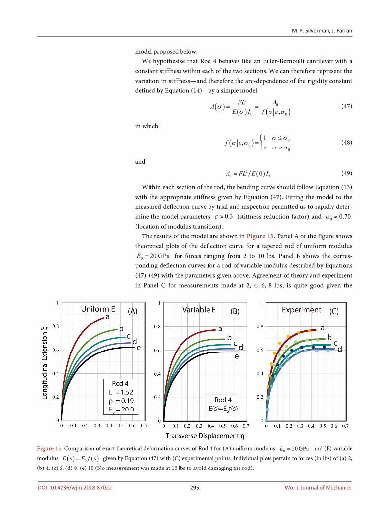
Within each section of the rod, the bending curve should follow Equation (13) with the appropriate stiffness given by Equation (47). Fitting the model to the measured deflection curve by trial and inspection permitted us to rapidly deter-mine the model parameters 0.3ε ≈ (stiffness reduction factor) and 0 0.70σ ≈ (location of modulus transition).

The results of the model are shown in Figure 13. Panel A of the figure shows theoretical plots of the deflection curve for a tapered rod of uniform modulus

0 20 GPaE = for forces ranging from 2 to 10 lbs. Panel B shows the corres-ponding deflection curves for a rod of variable modulus described by Equations (47)-(49) with the parameters given above. Agreement of theory and experiment in Panel C for measurements made at 2, 4, 6, 8 lbs, is quite good given the

Figure 13. Comparison of exact theoretical deformation curves of Rod 4 for (A) uniform modulus 0 20 GPaE = and (B) variable

modulus ( ) ( )0E s E f s= given by Equation (47) with (C) experimental points. Individual plots pertain to forces (in lbs) of (a) 2,

(b) 4, (c) 6, (d) 8, (e) 10 (No measurement was made at 10 lbs to avoid damaging the rod).

https://doi.org/10.4236/wjm.2018.87022



simplicity of the model. No measurements were made at 10 lbs to avoid possibly damaging the rods. Moreover, as shown by plots e and d in both Panels A and B, the theoretical deflection curve expected for a force of 10 lbs (plot e) does not differ significantly from the curve produced by a force of 8 lbs (plot d).

The deflection profiles of Rod 5 in Figure 12, show weakly anomalous beha-vior in a small section of the rod near the tip for the smaller applied forces of 2 and 4 lbs and excellent agreement again over the full length of the rod at the larger applied forces of 6 and 8 lbs. In contrast to the response of Rod 4, the de-formation curve of Rod 5 revealed the rod to be stiffer than expected theoreti-cally at the lower loads. Assuming, as before, that the cross section of the rod at any arc length remains circular, the features exhibited by Rod 5 suggest that the modulus E is greater in the end section. In other words, above some threshold force the modulus is uniform throughout the rod as indicated by the panels for W = 6, 8 lbs, but below threshold the rod behaves like an Euler-Bernoulli beam with different constant modulus in the front and rear sections.

We can account quantitatively for the observed features of Rod 5 by the same model as for Rod 4, but with different parameters. Fitting the exact theoretical calculations to the data by trial and inspection yielded a stiffness enhancement factor 2.9ε ≈ , and partition location 0 0.75σ ≈ , which gave very satisfactory results, as seen in Figure 14. Panel A of the figure shows the deflection curves (solid) as calculated exactly by Equation (13) with model (47) for the partitioned modulus, and the corresponding deflection curves (dotted) for the rod with uni-form modulus. Panel B shows the agreement (plots a and b) between the parti-tioned-modulus model and the deflection curves of Figure 12 measured for

Figure 14. Comparison of exact theoretical deformation curves of Rod 5 for (A) uniform modulus (dotted curve) 0 30 GPaE = and variable modulus (solid curve) ( ) ( )0E s E f s=

given by Equations (47) and (48) with (B) experimental points. Individual plots pertain to applied forces (in lbs) of (a) 2, (b) 4, (c) 6, (d) 8, (e) 10.

https://doi.org/10.4236/wjm.2018.87022



applied loads W of 2 and 4 pounds. Although the exact theory based on a uniform modulus in Rod 5 agreed very

well with the experimental deflection curves for W = 6 and 8 lbs, as shown in Figure 12, it is of interest to see how that agreement would be affected if the deflection curve were generated by the preceding two-section model. This com-parison is shown for W = 8 lbs by plot d in Panel B of Figure 14. The agreement with experiment is only marginally poorer than the excellent match shown in Figure 12 for a uniform load. This suggests the possibility that the modulus of Rod 5 may have a weak force dependence (without a threshold) that falls off ra-pidly with increasing W, thereby leading to no appreciable distortion of the def-lection curves for large W. Further investigation of the stress dependence of Rod 5, however, is outside the scope of this paper.

4. Conclusions

This paper reports a comprehensive theoretical analysis and experimental test of the static deflection of a tapered rod subject to an end load that can generate an arbitrarily large bending deformation, assuming the rod retains its circular cross section and linear elastic response. Large-scale and small-scale systems of this kind occur widely in modern physics. The calculation of the bending curve for this system leads to a non-linear second order differential equation for which a closed-form solution is unknown and which, therefore, must be solved numeri-cally. In this regard the choice of coordinate system is very important.

If the exact differential equation is expressed directly in terms of the desired Cartesian coordinates of the deflection curve (x = longitudinal extension; y = transverse displacement), the resulting equation contains a geometric parameter and dynamical relation that are unknown at the outset. Attempts to solve this equation iteratively by means of a powerful mathematical tool like Maple took long computation times and did not reliably converge to a solution. However, if the equation is expressed in terms of arc length s and tangent angle θ , then the resulting differential equation for ( )sθ contains only the single variable s without any unknown parameters. From the solution ( )sθ , the function ( )y x of the elastica was calculated rapidly by iterative numerical integration of equa-tions relating the derivatives d dx s and d dy s to ( )sθ . Using Maple, we were able to solve the deflection equation to 10-digit precision and calculate the exact elastica shape for each desired configuration of rod geometry, elastic mod-ulus, and applied force within a few seconds.

Comparison of the exact deflection curves of tapered and uniform rods of identical properties apart from taper showed, for a variety of rod geometries, elastic moduli, and loads, that neglect of tapering could result in greatly unde-restimating the extent of bending.

To test the elastica theory of a tapered rod, we recorded and analyzed the def-lection curves of a series of highly flexible rods with total lengths ranging from 6 feet (1.83 m) to 10 feet (3.05 m) and taper ratios ranging from 3:10 to 3:17. The

https://doi.org/10.4236/wjm.2018.87022



rods were made of various composites of fiberglass and resins designed to main-tain their circular cross sections under stress within elastic limits. Given their properties, we expected these rods to undergo moderate to large deflections when subjected to loads ranging from 2 lbs (8.90 N) to 8 lbs (35.59 N).

Our experimental results showed the following: • Excellent agreement was obtained between theory and experiment for all four

loads applied to the three shortest rods with three highest taper ratios (see Rods 1, 2, 3 in Table 1). Maximum deflection angles in all 12 cases (3 rods × 4 forces) ranged from about 70˚ to 90˚ which constituted very large deflec-tions for which neither the exact nonlinear theory for uniform rods (taper ra-tio = 1; theory solvable in terms of elliptic integrals) nor the widely used Eu-ler-Bernoulli approximate theory (which generates a 3rd order polynomial) is applicable. The difference in calculated tip deflection angles between the ta-pered rods and corresponding uniform rods ranged from about 5˚ to 65˚.

• Weakly discordant results were initially obtained between some of the theo-retically predicted shapes and the measured deflection curves of the longest two rods with lowest taper ratios (see Rods 4, 5 in Table 1). The anomalies could be understood as arising from a difference in flexural rigidity at the narrow end compared with that throughout the rest of the rod. A simple theoretical model was devised to yield the reduction or enhancement of rod stiffness and the transition location. Theoretical prediction of the elastica curves, taking account of the stiffness model, was in excellent accord with the measured deflection curves.

Although the stiffness model does not explain the physical mechanism for the bipartite modulus of Rods 4 and 5, the practical utility of our procedure is that it permits numerical prediction of virtually all the geometrical and physical prop-erties of the equilibrium cantilever configuration that an analyst, experimenter, or instrument designer might want to correlate with load, such as the overall shape (the elastica curve), maximum deflection angle, maximum linear deflec-tion, point of maximum curvature, bending moment, distribution of bending stress, and other quantities.

As a final point, we mention that in many applications on length scales rang-ing from fishing rods to micro-electromechanical devices there may be interest not only in the equilibrium configuration but also in the dynamical response of a tapered rod to a time-dependent perturbation. Although this subject is outside the scope of our paper, it is to be noted that the equations of static equilibrium analyzed here provide the starting point for an exact dynamical analysis, since, in the absence of a perturbation, the system relaxes to the equilibrium state. Al-though dynamical analyses have been performed on uniform cantilevers in the approximation of small-angle deflections [33], we are unaware of any exact dy-namical analysis of a tapered cantilever.

Acknowledgements

M. P. Silverman gratefully acknowledges the George A. Jarvis research fund for support of this project.

https://doi.org/10.4236/wjm.2018.87022



Conflicts of Interest

The authors declare no conflicts of interest regarding the publication of this pa-per.

References [1] Levien, R. (2008) The Elastica: A Mathematical History. Electrical Engineering and

Computer Sciences University of California at Berkeley Technical Report No. UCB/EECS 2008-103. http://www.eecs.berkeley.edu/Pubs/TechRpts/2008/EECS-2008-103.html

[2] Fertis, D.G. (2006) Nonlinear Structural Engineering with Unique Theories and Methods to Solve Effectively Complex Nonlinear Problems. Springer, New York, NY.

[3] Sarid, D. (1994) Scanning Force Microscopy with Applications to Electric, Magnet-ic, and Atomic Forces. Oxford University Press, Oxford, UK.

[4] Banica, F.G. (2012) Chemical Sensors and Biosensors: Fundamentals and Applica-tions. Wiley, New York, NY. https://doi.org/10.1002/9781118354162

[5] Timoshenko, S. (1934) Theory of Elasticity. McGraw-Hill, New York, NY, 33-42.

[6] Budynas, R.G. (1977) Advanced Strength and Applied Stress Analysis. McGraw-Hill, New York, NY, 508 p.

[7] Filonenko-Borodich, M. (1965) Theory of Elasticity. Dover Publications, New York, NY, 155-162.

[8] Zeng, D. and Zheng, Q. (2010) Large Deflection Theory of Nanobeams. Acta Me-chanica Solida Sinica, 23, 394-399. https://doi.org/10.1016/S0894-9166(10)60041-9

[9] Mutyalarao, M., Bharathi, D. and Rao, N. (2010) Large Deflections of a Cantilever Beam under an Inclined End Load. Applied Mathematics and Computation, 217, 3607-3613. https://doi.org/10.1016/j.amc.2010.09.021

[10] Tari, H. (2013) On the Parametric Large Deflection Study of Euler-Bernoulli Canti-lever Beams Subjected to Combined Tip Point Loading. International Journal of Non-Linear Mechanics, 49, 90-99. https://doi.org/10.1016/j.ijnonlinmec.2012.09.004

[11] Tari, H., Kinzel, G.L. and Mendelsohn, D.A. (2015) Cartesian and Piecewise Para-metric Large Deflection Solutions of Tip Point Loaded Euler-Bernoulli Cantilever Beams. International Journal of Mechanical Sciences, 100, 216-225. https://doi.org/10.1016/j.ijmecsci.2015.06.024

[12] Landau, L.D. and Lifshitz, E.M. (1970) Theory of Elasticity. Pergamon Press, New York, NY, 75-97.

[13] Bisshopp, K.E. and Drucker, D.C. (1945) Large Deflection of Cantilever Beams. Quarterly of Applied Mathematics, 3, 272-275. https://doi.org/10.1090/qam/13360

[14] Avitzur, B. (1985) Deflection in Tapered Cantilever Beams. Technical Report ARLCS-TR-85027, US Army Armament Research and Development Center, Wa-tervliet, NY.

[15] McCutcheon, W.J. (1983) Deflections and Stresses in Circular Tapered Beams and Poles. Civil Engineering for Practicing and Design Engineers, 2, 207-233.

[16] Kien, N.D. (2014) Large Displacement Behaviour of Tapered Cantilever Eu-ler-Bernoulli Beams Made of Functionally Graded Material. Applied Mathematics and Computation, 237, 340-355. https://doi.org/10.1016/j.amc.2014.03.104

https://doi.org/10.4236/wjm.2018.87022

http://www.eecs.berkeley.edu/Pubs/TechRpts/2008/EECS-2008-103.html

https://doi.org/10.1002/9781118354162

https://doi.org/10.1016/S0894-9166(10)60041-9

https://doi.org/10.1016/j.amc.2010.09.021

https://doi.org/10.1016/j.ijnonlinmec.2012.09.004

https://doi.org/10.1016/j.ijmecsci.2015.06.024

https://doi.org/10.1090/qam/13360

https://doi.org/10.1016/j.amc.2014.03.104



[17] Rajasekaran, S. and Khaniki, H.B. (2017) Bending, Buckling, and Vibration of Small-Scale Tapered Beams. International Journal of Engineering Science, 120, 172-188. https://doi.org/10.1016/j.ijengsci.2017.08.005

[18] Kemper, J.D. (1968) Large Deflections of Tapered Cantilever Beams. International Journal of Mechanical Sciences, 10, 469-478.

[19] Hibbeler, R.C. (1997) Mechanics of Materials. 3rd Edition, Prentice Hall, Upper Saddle River, NJ, USA, 855 p.

[20] Stippes, M., Wempner, G., Stern, M. and Beckett, R. (1961) The Mechanics of De-formable Bodies. Charles E. Merrill Books Inc., Columbus, OH, USA, 240-244.

[21] Struik, D.J. (1961) Lecture on Classical Differential Geometry. Addison-Wesley, Reading, MA, USA, 74-77.

[22] Isaacson, E. and Keller, H.B. (1966) Analysis of Numerical Methods. Wiley, New York, 367-374.

[23] Sirca, S. and Horvat, M. (2012) Computational Methods for Physicists. Springer, Heidelberg, Germany, 716 p. https://doi.org/10.1007/978-3-642-32478-9

[24] Maple User Manual (2012) Maplesoft. McKinney, TX, USA, 378-381.

[25] Silverman, M.P. (2017) Brownian Motion of Decaying Particles: Transition Proba-bility, Computer Simulation, and First-Passage Times. Journal of Modern Physics, 8, 1809-1849. https://doi.org/10.4236/jmp.2017.811108

[26] Goldstein, H. (1980) Classical Mechanics. Addison-Wesley, Reading, MA, USA, 16-21, 339-347.

[27] Callen, H.B. (1960) Thermodynamics: An Introduction to the Physical Theories of Equilibrium Thermostatics and Irreversible Thermodynamics. Wiley, New York, NY, 90-98. https://doi.org/10.1115/1.3644060

[28] Phillips, D. (2000) The Technology of Fly Rods: An In-Depth Look at the Design of the Modern Fly Rod, Its History and Its Role in Fly Fishing. Frank Amato Publica-tions, Portland, OR, USA.

[29] http://www.allfishingbuy.com/Fishing-Rods-Materials.htm

[30] Tracker Image Analysis Software Home Page. https://physlets.org/tracker/

[31] Silverman, M.P. (2014) A Certain Uncertainty: Nature’s Random Ways. Cambridge University Press, Cambridge, UK, 54-66. https://doi.org/10.1017/CBO9781139507370

[32] Monahan, P. (2013) Understanding Rod Action and Choosing the Right Rod for You. https://news.orvis.com/fly-fishing/Understanding-Rod-Action

[33] Ashhab, M., Salapaka, M.V., Dahleh, M. and Mezic, I. (1999) Dynamical Analysis and Control of Microcantilevers. Automatica, 35, 1663-1670. https://doi.org/10.1016/S0005-1098(99)00077-1

https://doi.org/10.4236/wjm.2018.87022

https://doi.org/10.1016/j.ijengsci.2017.08.005

https://doi.org/10.1007/978-3-642-32478-9

https://doi.org/10.4236/jmp.2017.811108

https://doi.org/10.1115/1.3644060

http://www.allfishingbuy.com/Fishing-Rods-Materials.htm

https://physlets.org/tracker/

https://doi.org/10.1017/CBO9781139507370

https://news.orvis.com/fly-fishing/Understanding-Rod-Action

https://doi.org/10.1016/S0005-1098(99)00077-1

Bending of a Tapered Rod: Modern Application and ... · equilibrium is known for the deflection of a tapered rod. We report in this paper a comprehensive numerical analysis and experimental

Documents