Benchmarking high order finite element approximations for one-dimensional boundary layer problems

Benchmarking high order finite element approximations forone-dimensional boundary layer problems

Marcello Malagu1,2, Elena Benvenuti1, Angelo Simone2

1Department of Engineering, University of Ferrara, ItalyE-mail: [email protected], [email protected]

2Faculty of Civil Engineering and Geosciences, Delft University of Technology, The NetherlandsE-mail: [email protected]

Keywords: FEM, B-spline, C∞ GFEM, boundary layers.

SUMMARY. In this article we investigate the application of high order approximation techniques toone-dimensional boundary layer problems. In particular, we use second order differential equationsand coupled second order differential equations as case studies. The accuracy and convergence rateof numerical solution obtained with Lagrange, Hermite, B-spline finite elements and C∞ generalizedfinite elements is assessed against analytical solutions.

1 INTRODUCTIONThe aim of this paper is to compare high order finite element approximation techniques in the

solution of classical engineering problems which exhibit boundary layers. In particular, we considerthe one-dimensional diffusion-transport-reaction equation whose weak and discrete formulations aredescribed in Section 2.

The analysis of transport (or advection) dominated problems with the traditional finite elementmethods (FEM) is computationally burdensome and more convenient approaches have been pro-posed [1]. Among the others, Hughes et al. [2] applied higher-order Non-Uniform Rational B-spline(NURBS) basis functions to advection-diffusion problems. In particular, it was observed that thequality of the numerical solutions improved with the oder of the basis functions. Thus, higher orderbasis functions could represent a strategic approach to solve diffusion problems with sharp boundarylayers [3].

In this contribution, we use B-spline and C∞ GFEM approximations along with classical La-grange and Hermite basis functions. B-spline basis functions, widely used in Isogeometric Analy-sis [2], are piecewise polynomials which yield smooth and high order basis functions, of arbitraryorder, on compact supports. This technique can achieve a high degree of continuity through theso-called k-refinement technique as described in Section 3.1. C∞ shape functions (C∞ GFEM) wereintroduced by Edwards [4] who proposed to employ a meshfree-like approach defined on a standardfinite element grid as detailed in Section 3.2. With reference to the discrete form of the diffusion-transport-reaction equation described in Section 2, the pull-out problem and the electro-kinetic prob-lem are numerically investigated in Section 4 and 5, respectively. Further, the advection-diffusionequation is investigated by making use of the standard Gelerkin method and the Galerkin Least-Squares (GLS) method in Section 6.

2 DIFFUSION-TRANSPORT-REACTION EQUATIONLet Ω be a one-dimensional domain with the boundary Γ divided into a natural (Γu) and an es-

sential (Γt ) part such that Γu∪Γt = Γ and Γu∩Γt = 0. The strong form of the problem corresponding

1

to the diffusion-transport-reaction equation is stated as:

− (au,x),x + bu,x + cu = f in Ω,

u = u on Γu, (1)t = au,x = t on Γt ,

where the subscript x preceded by a comma denotes differentiation with respect to x itself, u is theunknown field and a, b, c and f are given functions (or constants). As in many applications, if theratio between the the transport term b or the reaction term c and the diffusion term a is much greaterthan one, the solution of (1) presents boundary layers.

Seeking for the approximate solution of the problem by the finite element method, the weak formof the problem statement is posed as follows:

find u ∈ U | (au,x, v,x)Ω + (bu,x, v)Ω + (cu, v)Ω = ( f , v)Ω − (au,x, v)Γt∀v ∈ V , (2)

where (·, ·)Ω denotes the L2-inner product on Ω, whereas U and V are the trial solutions spaceand the weighting functions space, respectively, such that U = u|u ∈ H1, u = u onΓu and V =v|v ∈ H1, v = 0 on Γu.

Referring to the Galerkin FEM, we approximate the trial functions u and the weight functions vby means of uh ∈ Uh = uh|uh ∈ H1, uh = u onΓu and vh ∈ Vh = vh|vh ∈ H1, vh = 0 on Γu,respectively. Thus, the finite element formulation of (1) is:

find uh ∈ Uh |(auh,x, vh,x

)Ω +

(buh,x, vh

)Ω + (cuh, vh)Ω = ( f , vh)Ω −

(auh,x, vh

)Γt∀vh ∈ Vh.

(3)However, solutions of diffusion problems obtained with the Galerkin method usually show oscilla-tions which vanish only with a large number of elements [1].

In order to improve the quality of the classical finite element method, the Galerkin Least-Squaresmethod stabilizes the numerical approximation of problem by adding a further term in the Galerkinformulation (3). By making reference to [1], the discretized GLS formulation of the diffusion-transport-reaction equation reads:

find uh ∈ Uh |(auh,x, vh,x

)Ω +

(buh,x, vh

)Ω + (cuh, vh)Ω +(

−auh,xx +buh,x + cuh, τ(−avh,xx +bvh,x + cvh))

Ω = ( f , vh)Ω −(auh,x, vh

)Γt+(

−auh,xx +buh,x + cuh, τ(−avh,xx +bvh,x + cvh))

Ω ∀vh ∈ Vh. (4)

In the above equation, the stabilization parameter

τ =h

2|b|min(

1,|b|

6|a|p2

), (5)

where h is the finite element size and p the polynomial order of the basis functions [5].

3 HIGH ORDER APPROXIMATIONS SCHEMES3.1 B-spline basis functions

B-splines are piecewise polynomial functions which can be used to construct higher order andcontinuous basis functions on compact supports. Each support is spanned by a sequence of coordi-nates, known as knots, which is related to the basis functions number n and order p. The knot set

2

Ξ = ξ1, ξ2, ..., ξn+p+1, termed knot vector, subdivides the domain into n+ p knot spans which areequivalent to the element domains of a standard finite element mesh. Once the basis functions oforder p and the knot vector Ξ are known, B-spline basis functions Ni,p are defined by means of theCox-de Boor recursion formula [2]. These basis functions form a partition of unity and they are non-negative over the whole domain. B-spline basis functions are usually Cp+1-continuous over theirsupport which is defined by p+1 knot spans. However, if a knot has multiplicity m, the continuityof the basis functions will decrease to Cp−m at that knot.

The quality of the approximation can be improved by employing h-refinement and p-refinementwhich are similar to the corresponding techniques used in the traditional finite element method.A combination of these two techniques, the so-called k-refinement, is a distinguishing feature ofB-spline basis functions. With this refinement scheme, order elevation and knots insertion are per-formed at the same time. In particular, this strategy leads to a periodic, sometimes referred to ashomogeneous, set of highly continuous basis functions [2].

3.2 C∞ GFEMThe C∞ generalized finite element method was proposed by Edwards [4] in order to build finite

elements with arbitrarily smooth basis functions. In C∞ GFEM, highly continuous basis functions,similar to those used in meshfree methods, have support on a standard finite element mesh. Inparticular, all finite elements sharing node xα define a polygonal region ωα called cloud. In a one-dimensional setting, ωα reduces to the portion of domain between nodes xα−1 and xα+1.

The construction of C∞ basis functions requires several accessory functions and starts with thedefinition of the cloud boundary functions

Eα, j(x) =

e−ξ

−γ

j ξ j > 00 otherwise,

(6)

which are defined on the support cloud ωα . The parametric coordinate

ξ j =

(1−2γ

loge β

) 1γ (x− x j)

hα j, (7)

where j is equal to α±1 and hα j is the distance between nodes xα and x j (we assume γ = 0.6 andβ = 0.3 [6]). These cloud boundary functions are used to define the weighting functions

Wα(x) = ecα

Mα

∏j=1

Eα, j(x) with cα = Mα

(1−2γ

loge β

)−1

, (8)

where the parameter Mα indicates the number of cloud boundary functions supported on ωα . C∞

partition of unity functions ϕα(x) at node xα are constructed through the Shepard’s formula usingthe weighting functions Wα(x) according to

ϕα(x) =Wα(x)

∑κ(x)Wκ(x)with κ(x) ∈ γ|Wγ(x) 6= 0. (9)

As shown in [6], C∞ basis functions satisfy the Kronecker delta property ϕα(xβ ) = δαβ . Finally,C∞ GFEM basis functions φαi(x) of order i at node xα are defined as the product of C∞ partition ofunity functions ϕα(x) and polynomial enrichments Lαi(x) as

φαi(x) = ϕα(x)Lαi(x) with Lαi(x) =(x− xα)

i

hα

, (10)

3

where hα is the cloud radius. For one-dimensional uniform meshes, like those used in this work,hα is the finite elements size. The basis functions φαi are employed to approximate the unknownsolution according to

u(x) wn

∑α=1

pα

∑i=0

uαiφαi(x) =n

∑α=1

pα

∑i=0

uαiLαi(x)ϕα(x) (11)

in which pα is the order of the polynomial enrichment function and, at the same time, indicatesthe number of degrees of freedom at node xα . From (10)-(11), Dirichlet boundary condition canbe enforced as in traditional finite element methods on the degree of freedom corresponding to thepolynomial enrichment of order zero [6].

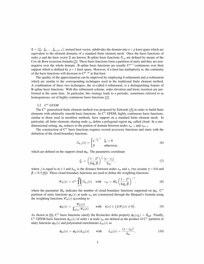
4 PULL-OUT PROBLEMThe governing equations of a simple one-dimensional pull-out problem can be derived from (1)

by assuming a as the product between the cross sectional area A and the elastic modulus E of thefiber, c as the rate of softening k with respect to sliding, and by setting the parameters b and f equalto zero. Furthermore, in this study case we make use of the boundary conditions t|0 = 1 kN andu|L = 0 m, where L is the fiber length. The exact solution of the problem is expressed as

u(x) =

(1+ e2

√ε(L−x)

)e√

εx

EA(2e2√

εL +1)√

ε, (12)

where ε = k/EA = a/c controls the boundary layer at the origin of the domain. In order to test thedifferent approximation techniques we set A = 1 m2, E = 1 Pa and k = 104 N. The problem is solvedby means of B-spline finite elements and C∞ GFEM along with the classical Lagrange and Hermitefinite elements. Furthermore, we discretize the domain with meshes of uniform density.

The numerical solutions computed with 25 degrees of freedom (dofs) present oscillations close tothe left boundary point as illustrated in Figure 1. These spurious oscillations depend on the approx-imation scheme. Lagrange basis functions yield steep oscillations at interelement boundaries due tothe C0 approximation of u(x). High order Hermite and B-spline basis functions improve consider-ably the results. In particular, septic Hermite Basis functions and quartic B-spline basis functionslead to almost monotone approximations. Despite the high continuity of the basis functions, C∞

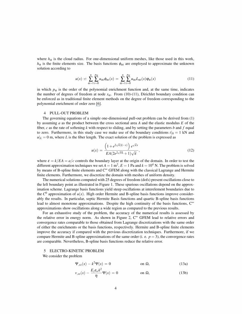
approximations show oscillations along a wide region as compared to the previous results.For an exhaustive study of the problem, the accuracy of the numerical results is assessed by

the relative error in energy norm. As shown in Figure 2, C∞ GFEM lead to relative errors andconvergence rates comparable to those obtained from Lagrange discretizations with the same orderof either the enrichments or the basis functions, respectively. Hermite and B-spline finite elementsimprove the accuracy if compared with the previous discretization techniques. Furthermore, if wecompare Hermite and B-spline approximations of the same order (i. e. p = 3), the convergence ratesare comparable. Nevertheless, B-spline basis functions reduce the relative error.

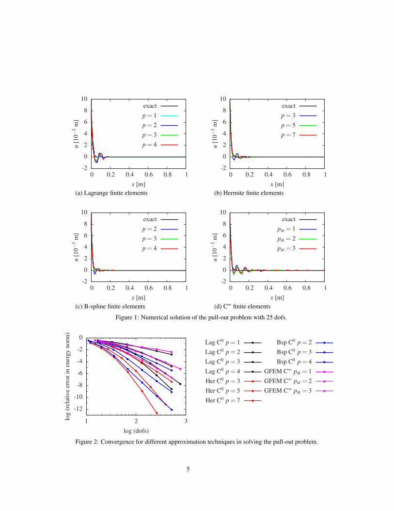
5 ELECTRO-KINETIC PROBLEMWe consider the problem

Ψ,xx(x) − k2Ψ(x) = 0 on Ω, (13a)

v,xx(x) −Ezεwk2

ηΨ(x) = 0 on Ω, (13b)

4

p = 7p = 5p = 3exact

x [m]

u[1

0−3

m]

10.80.60.40.20

10

8

6

4

2

0

-2

pα = 3pα = 2pα = 1

exact

x [m]

u[1

0−3

m]

10.80.60.40.20

10

8

6

4

2

0

-2

p = 4p = 3p = 2p = 1exact

x [m]

u[1

0−3

m]

10.80.60.40.20

10

8

6

4

2

0

-2

p = 4p = 3p = 2exact

x [m]

u[1

0−3

m]

10.80.60.40.20

10

8

6

4

2

0

-2

GFEM C∞ pα = 3GFEM C∞ pα = 2GFEM C∞ pα = 1

Bsp C0 p = 4Bsp C0 p = 3Bsp C0 p = 2

Her C0 p = 7Her C0 p = 5Her C0 p = 3Lag C0 p = 4Lag C0 p = 3Lag C0 p = 2Lag C0 p = 1

log (dofs)

log

(rel

ativ

eer

rori

nen

ergy

norm

)

321

0

-2

-4

-6

-8

-10

-12

(a) Lagrange finite elements (b) Hermite finite elements

(d) C∞ finite elements

Figure 1: Numerical solution of the pull-out problem with 25 dofs.

(c) B-spline finite elements

Figure 2: Convergence for different approximation techniques in solving the pull-out problem.

5

p = 4p = 3p = 2p = 1exact

x [m]

v[1

06m

/s]

0.050.040.030.020.010

0

-2

-4

-6

-8

-10

p = 7p = 5p = 3exact

x [m]

v[1

06m

/s]

0.050.040.030.020.010

0

-2

-4

-6

-8

-10

p = 7p = 5p = 3exact

x [m]

v[1

06m

/s]

0.050.040.030.020.010

2

0

-2

-4

-6

-8

-10

pα = 3pα = 2pα = 1

exact

x [m]

v[1

06m

/s]

0.050.040.030.020.010

0

-2

-4

-6

-8

-10

GFEM C∞ pα = 3GFEM C∞ pα = 2GFEM C∞ pα = 1

Bsp C3 p = 4Bsp C2 p = 3Bsp C1 p = 2

Her C3 p = 7Her C2 p = 5Her C1 p = 3Lag C0 p = 4Lag C0 p = 3Lag C0 p = 2Lag C0 p = 1

log (dofs)

log

(rel

ativ

eer

rori

nen

ergy

norm

)

321

0

-2

-4

-6

-8

-10

-12

(a) Lagrange finite elements (b) Hermite finite elements

(d) C∞ finite elements(c) B-spline finite elementsFigure 3: Numerical solution of the electro-kinetic problem with 25 dofs (only half of the solution is

plotted due simmetry).

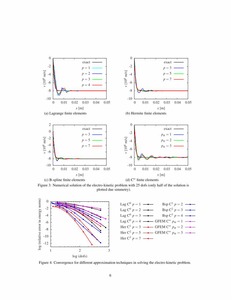
Figure 4: Convergence for different approximation techniques in solving the electro-kinetic problem.

6

which describes the relation between the electrostatic potential Ψ of a liquid between two electricallycharged walls and its velocity v induced by the electro-osmosis process [7]. We observe that bothequations in (13) can be easily derived from (1). Namely, (13a) is a diffusion-reaction equation(b = 0) whereas (13b) is a diffusion equation (b = c = 0). The constant k is the Debye-Huckelparameter, Ez the electric field strength, εw the water permittivity and η the viscosity of the fluid. Byassuming Ψ|0,L = Ψ0 = 1 V and v|0,L = 0 m/s, the exact solution of the problem is defined by

Ψ(x) = Ψ0(1− e−kL)ekx − (1− ekL)e−kx

(ekL− e−kL)and (14a)

v(x) =Ezεw

η(Ψ(x)−Ψ0) . (14b)

The electrostatic potential Ψ and the fluid velocity v present boundary layers when k has high value.Here, we assume k = 103 m−1, Ez = 100 N/C, εw = 80.1 and η = 1.002 mPa s. Once again, thedomain is discretized with a uniform mesh.

The numerical approximations of Ψ(x) (omitted for the sake of brevity) present oscillations atthe boundaries. These results are in agreement with those computed in Section 4 since (13a) isa diffusion-reaction equation. Moreover, also the approximations of v(x) illustrated in Figure 3present similar oscillations. Finally, since the relative error in energy norm depends on the error inapproximating both Ψ(x) and v(x), the convergence rates shown in Figure 4 are comparable withthose in Figure 2.

6 ADVECTION-DIFFUSION EQUATIONThe advection-diffusion equation is easily derived from (1) by neglecting the reaction term c.

Hence, if we assume f = 1 K/m2and the boundary conditions u|0,L = 0 K, the exact solution of theproblem is expressed by

u(x) =1v

(x− 1− ePex

1− ePe

), (15)

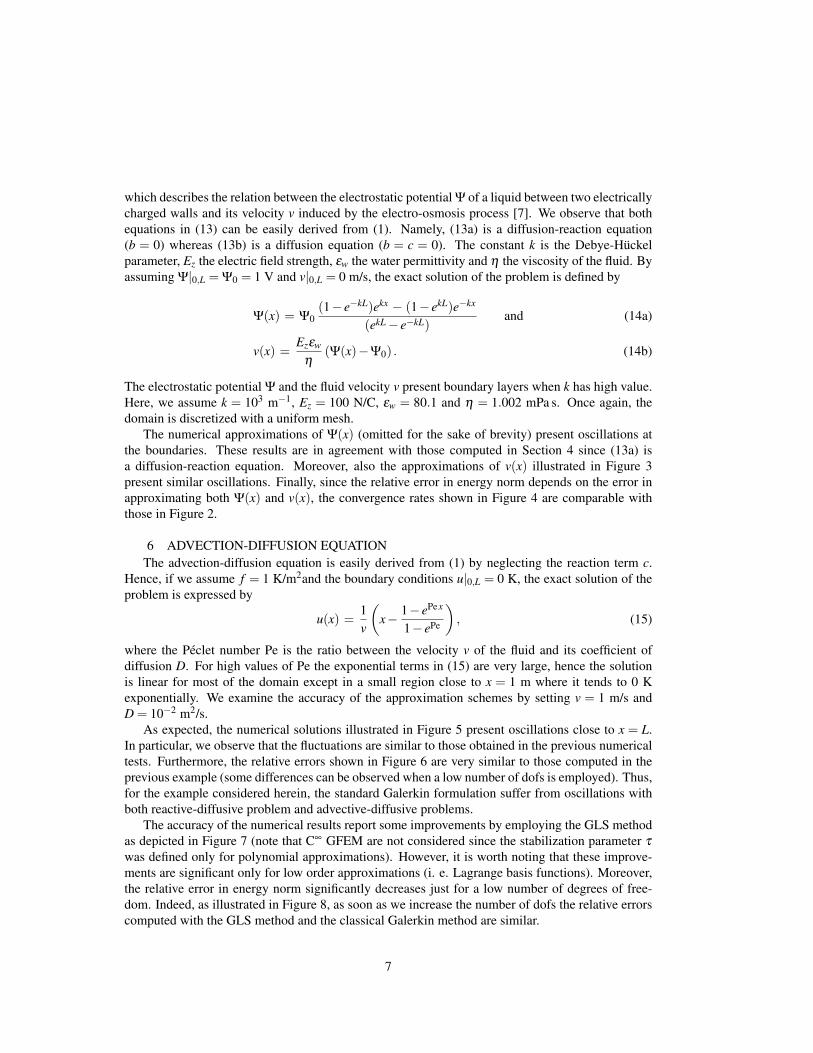
where the Peclet number Pe is the ratio between the velocity v of the fluid and its coefficient ofdiffusion D. For high values of Pe the exponential terms in (15) are very large, hence the solutionis linear for most of the domain except in a small region close to x = 1 m where it tends to 0 Kexponentially. We examine the accuracy of the approximation schemes by setting v = 1 m/s andD = 10−2 m2/s.

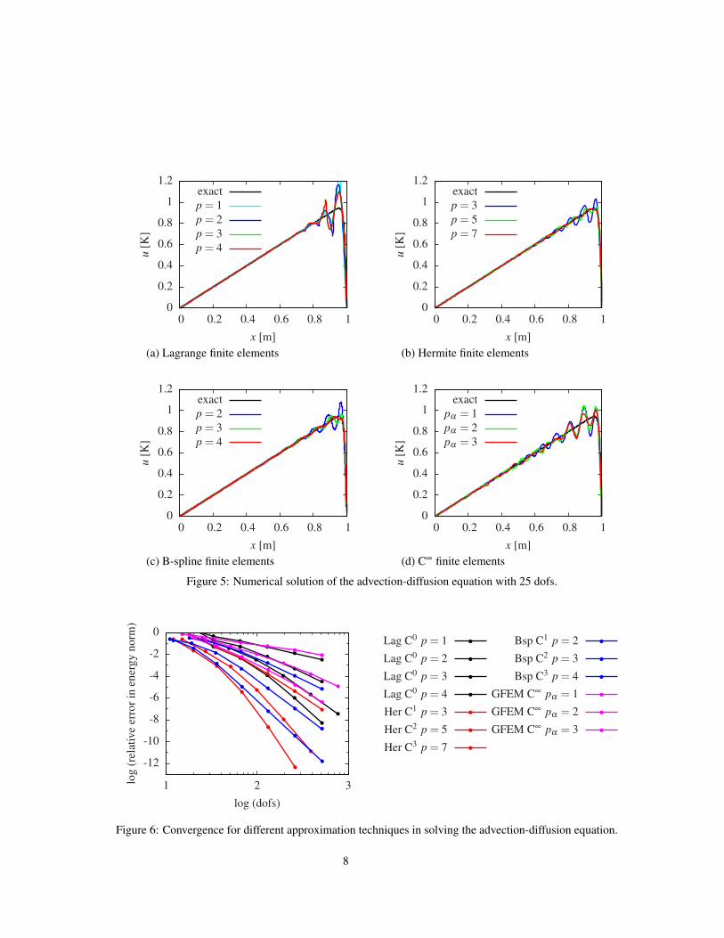
As expected, the numerical solutions illustrated in Figure 5 present oscillations close to x = L.In particular, we observe that the fluctuations are similar to those obtained in the previous numericaltests. Furthermore, the relative errors shown in Figure 6 are very similar to those computed in theprevious example (some differences can be observed when a low number of dofs is employed). Thus,for the example considered herein, the standard Galerkin formulation suffer from oscillations withboth reactive-diffusive problem and advective-diffusive problems.

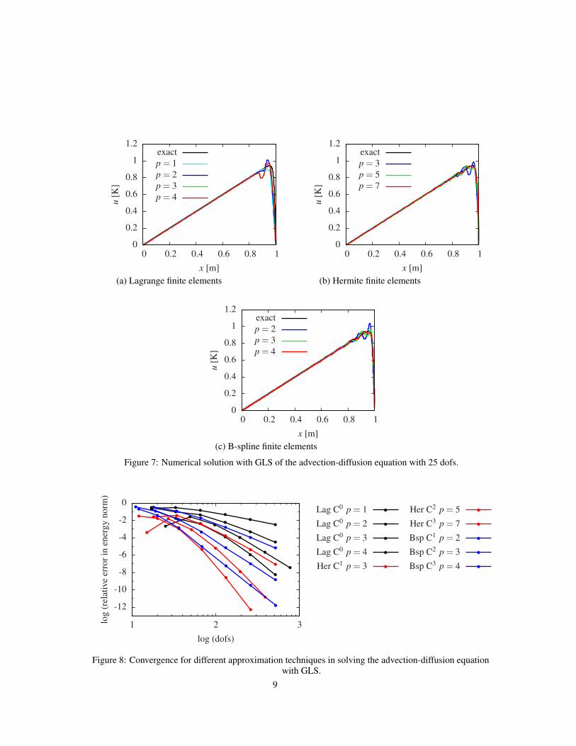
The accuracy of the numerical results report some improvements by employing the GLS methodas depicted in Figure 7 (note that C∞ GFEM are not considered since the stabilization parameter τ

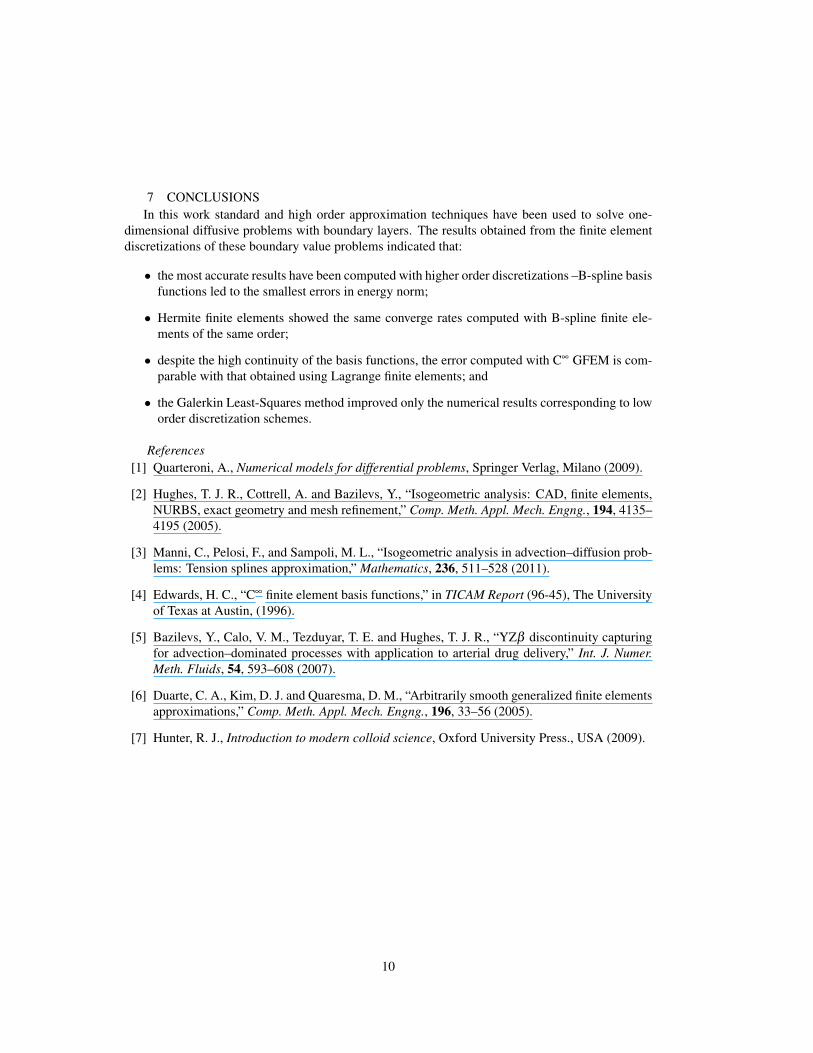
was defined only for polynomial approximations). However, it is worth noting that these improve-ments are significant only for low order approximations (i. e. Lagrange basis functions). Moreover,the relative error in energy norm significantly decreases just for a low number of degrees of free-dom. Indeed, as illustrated in Figure 8, as soon as we increase the number of dofs the relative errorscomputed with the GLS method and the classical Galerkin method are similar.

7

GFEM C∞ pα = 3GFEM C∞ pα = 2GFEM C∞ pα = 1

Bsp C3 p = 4Bsp C2 p = 3Bsp C1 p = 2

Her C3 p = 7Her C2 p = 5Her C1 p = 3Lag C0 p = 4Lag C0 p = 3Lag C0 p = 2Lag C0 p = 1

log (dofs)

log

(rel

ativ

eer

rori

nen

ergy

norm

)

321

0

-2

-4

-6

-8

-10

-12

p = 4p = 3p = 2p = 1exact

x [m]

u[K

]

10.80.60.40.20

1.2

1

0.8

0.6

0.4

0.2

0

p = 7p = 5p = 3exact

x [m]

u[K

]

10.80.60.40.20

1.2

1

0.8

0.6

0.4

0.2

0

p = 4p = 3p = 2exact

x [m]

u[K

]

10.80.60.40.20

1.2

1

0.8

0.6

0.4

0.2

0

pα = 3pα = 2pα = 1

exact

x [m]

u[K

]

10.80.60.40.20

1.2

1

0.8

0.6

0.4

0.2

0

Figure 6: Convergence for different approximation techniques in solving the advection-diffusion equation.

(a) Lagrange finite elements (b) Hermite finite elements

Figure 5: Numerical solution of the advection-diffusion equation with 25 dofs.

(c) B-spline finite elements (d) C∞ finite elements

8

p = 4p = 3p = 2p = 1exact

x [m]

u[K

]

10.80.60.40.20

1.2

1

0.8

0.6

0.4

0.2

0

p = 7p = 5p = 3exact

x [m]

u[K

]

10.80.60.40.20

1.2

1

0.8

0.6

0.4

0.2

0

p = 4p = 3p = 2exact

x [m]

u[K

]

10.80.60.40.20

1.2

1

0.8

0.6

0.4

0.2

0

Bsp C3 p = 4Bsp C2 p = 3Bsp C1 p = 2Her C3 p = 7Her C2 p = 5

Her C1 p = 3Lag C0 p = 4Lag C0 p = 3Lag C0 p = 2Lag C0 p = 1

log (dofs)

log

(rel

ativ

eer

rori

nen

ergy

norm

)

321

0

-2

-4

-6

-8

-10

-12

(a) Lagrange finite elements (b) Hermite finite elements

(c) B-spline finite elements

with GLS.Figure 8: Convergence for different approximation techniques in solving the advection-diffusion equation

Figure 7: Numerical solution with GLS of the advection-diffusion equation with 25 dofs.

9

7 CONCLUSIONSIn this work standard and high order approximation techniques have been used to solve one-

dimensional diffusive problems with boundary layers. The results obtained from the finite elementdiscretizations of these boundary value problems indicated that:

• the most accurate results have been computed with higher order discretizations –B-spline basisfunctions led to the smallest errors in energy norm;

• Hermite finite elements showed the same converge rates computed with B-spline finite ele-ments of the same order;

• despite the high continuity of the basis functions, the error computed with C∞ GFEM is com-parable with that obtained using Lagrange finite elements; and

• the Galerkin Least-Squares method improved only the numerical results corresponding to loworder discretization schemes.

References[1] Quarteroni, A., Numerical models for differential problems, Springer Verlag, Milano (2009).

[2] Hughes, T. J. R., Cottrell, A. and Bazilevs, Y., “Isogeometric analysis: CAD, finite elements,NURBS, exact geometry and mesh refinement,” Comp. Meth. Appl. Mech. Engng., 194, 4135–4195 (2005).

[3] Manni, C., Pelosi, F., and Sampoli, M. L., “Isogeometric analysis in advection–diffusion prob-lems: Tension splines approximation,” Mathematics, 236, 511–528 (2011).

[4] Edwards, H. C., “C∞ finite element basis functions,” in TICAM Report (96-45), The Universityof Texas at Austin, (1996).

[5] Bazilevs, Y., Calo, V. M., Tezduyar, T. E. and Hughes, T. J. R., “YZβ discontinuity capturingfor advection–dominated processes with application to arterial drug delivery,” Int. J. Numer.Meth. Fluids, 54, 593–608 (2007).

[6] Duarte, C. A., Kim, D. J. and Quaresma, D. M., “Arbitrarily smooth generalized finite elementsapproximations,” Comp. Meth. Appl. Mech. Engng., 196, 33–56 (2005).

[7] Hunter, R. J., Introduction to modern colloid science, Oxford University Press., USA (2009).

10