Part 6: Core Theory II: Bellman Equations and Dynamic Programming Introduction to Reinforcement Learning

Welcome message from author
This document is posted to help you gain knowledge. Please leave a comment to let me know what you think about it! Share it to your friends and learn new things together.
Transcript
Part 6: Core Theory II: Bellman Equations and Dynamic
Programming
Introduction to Reinforcement Learning
Bellman Equations Recursive relationships among values that can be used to compute values

The tree of transition dynamicsa path, or trajectory
state
action
possible path
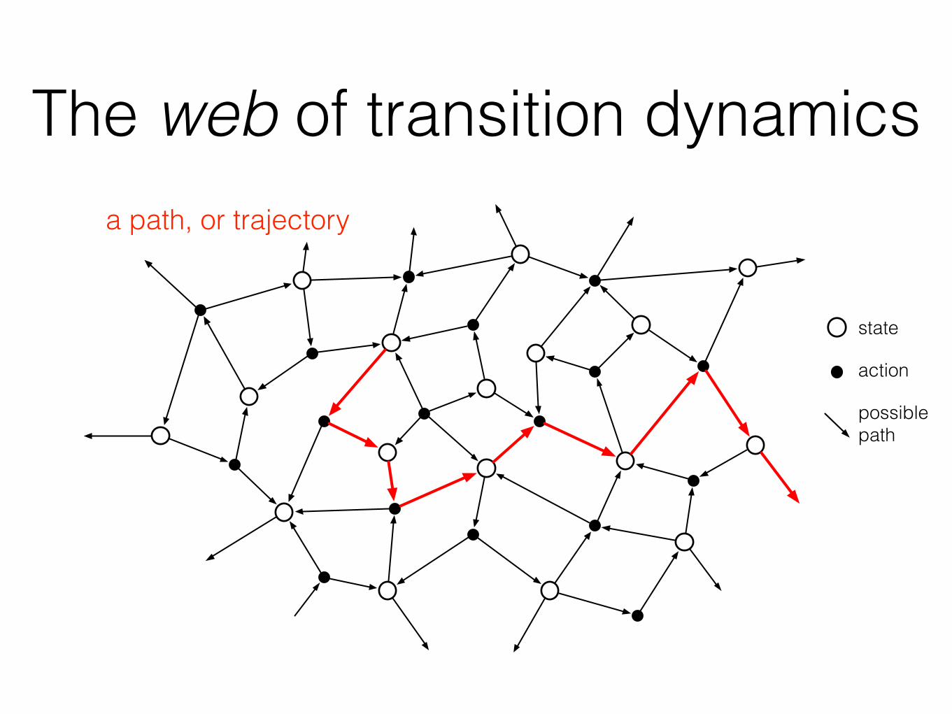
The web of transition dynamicsa path, or trajectory
state
action
possible path
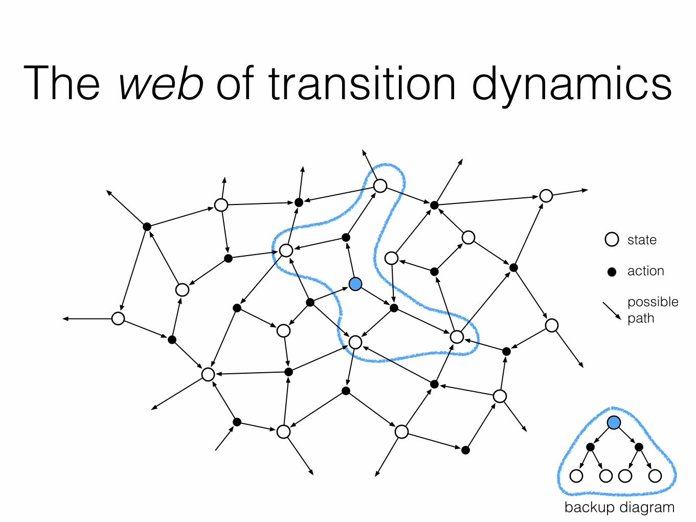
The web of transition dynamics
backup diagram
state
action
possible path
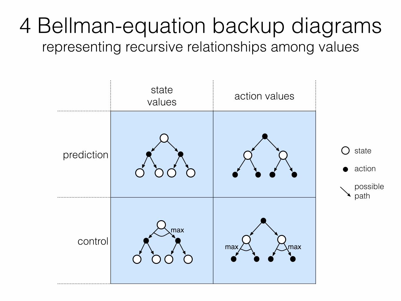
4 Bellman-equation backup diagrams representing recursive relationships among values
state values action values
prediction
controlmax
max max
state
action
possible path

R. S. Sutton and A. G. Barto: Reinforcement Learning: An Introduction 10
Bellman Equation for a Policy π
Gt = Rt+1 + γ Rt+2 + γ2Rt+3 + γ
3Rt+4L= Rt+1 + γ Rt+2 + γ Rt+3 + γ
2Rt+4L( )= Rt+1 + γGt+1
The basic idea:
So: vπ (s) = Eπ Gt St = s{ }= Eπ Rt+1 + γ vπ St+1( ) St = s{ }
Or, without the expectation operator:
...+
...+
v⇡(s) =X
a
⇡(a|s)X
s0,r
p(s0, r|s, a)hr + �v⇡(s
0)i
v⇡(s) = E⇡
⇥Rt+1 + �Rt+2 + �2Rt+3 + · · ·
�� St=s⇤
= E⇡[Rt+1 + �v⇡(St+1) | St=s] (1)
=X
a
⇡(a|s)X
s0,r
p(s0, r|s, a)hr + �v⇡(s
0)i, (2)
i
R. S. Sutton and A. G. Barto: Reinforcement Learning: An Introduction 11
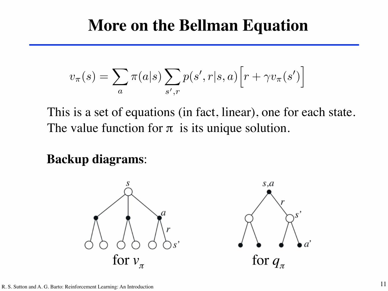
More on the Bellman Equation
This is a set of equations (in fact, linear), one for each state.The value function for π is its unique solution.
Backup diagrams:
for vπ for qπ
v⇡(s) =X
a
⇡(a|s)X
s0,r
p(s0, r|s, a)hr + �v⇡(s
0)i
v⇡(s) = E⇡
⇥Rt+1 + �Rt+2 + �2Rt+3 + · · ·
�� St=s⇤
= E⇡[Rt+1 + �v⇡(St+1) | St=s] (1)
=X
a
⇡(a|s)X
s0,r
p(s0, r|s, a)hr + �v⇡(s
0)i, (2)
i
R. S. Sutton and A. G. Barto: Reinforcement Learning: An Introduction 12
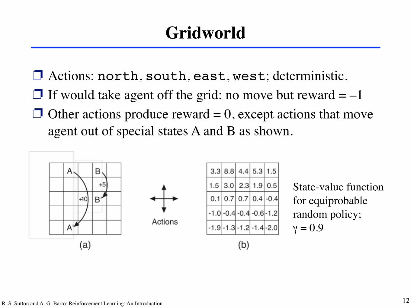
Gridworld
❐ Actions: north, south, east, west; deterministic.❐ If would take agent off the grid: no move but reward = –1❐ Other actions produce reward = 0, except actions that move
agent out of special states A and B as shown.
State-value function for equiprobable random policy;γ = 0.9
R. S. Sutton and A. G. Barto: Reinforcement Learning: An Introduction 13
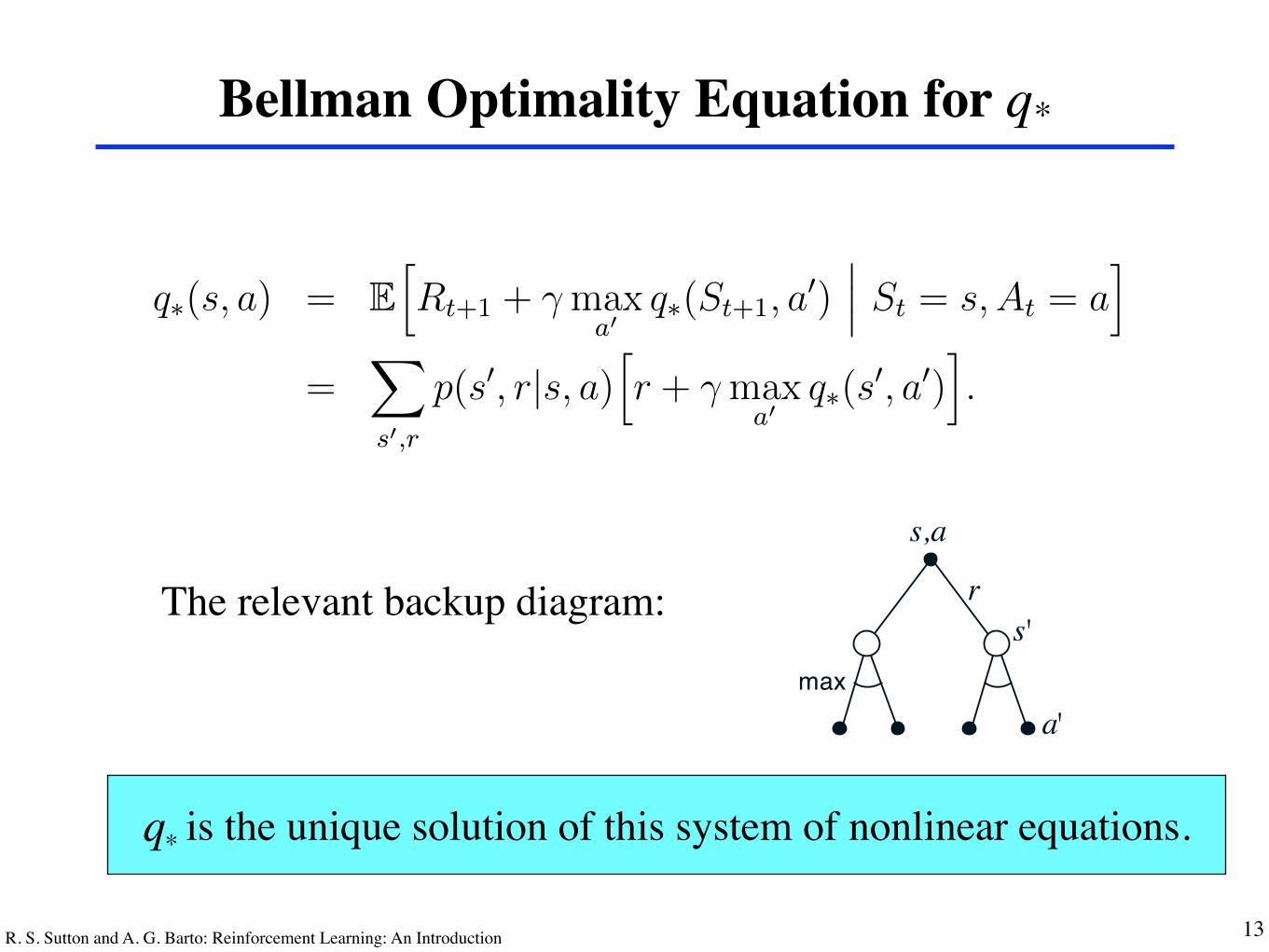
Bellman Optimality Equation for q*
The relevant backup diagram:
is the unique solution of this system of nonlinear equations.q*
s,as
a
s'
r
a'
s'
r
(b)(a)
max
max
68 CHAPTER 3. THE REINFORCEMENT LEARNING PROBLEM
q⇤(s, driver). These are the values of each state if we first play a stroke withthe driver and afterward select either the driver or the putter, whichever isbetter. The driver enables us to hit the ball farther, but with less accuracy.We can reach the hole in one shot using the driver only if we are already veryclose; thus the �1 contour for q⇤(s, driver) covers only a small portion ofthe green. If we have two strokes, however, then we can reach the hole frommuch farther away, as shown by the �2 contour. In this case we don’t haveto drive all the way to within the small �1 contour, but only to anywhereon the green; from there we can use the putter. The optimal action-valuefunction gives the values after committing to a particular first action, in thiscase, to the driver, but afterward using whichever actions are best. The �3contour is still farther out and includes the starting tee. From the tee, the bestsequence of actions is two drives and one putt, sinking the ball in three strokes.
Because v⇤ is the value function for a policy, it must satisfy the self-consistency condition given by the Bellman equation for state values (3.12).Because it is the optimal value function, however, v⇤’s consistency conditioncan be written in a special form without reference to any specific policy. Thisis the Bellman equation for v⇤, or the Bellman optimality equation. Intuitively,the Bellman optimality equation expresses the fact that the value of a stateunder an optimal policy must equal the expected return for the best actionfrom that state:
v⇤(s) = maxa2A(s)
q⇡⇤(s, a)
= maxa
E⇡⇤[Gt | St =s, At =a]
= maxa
E⇡⇤
" 1X
k=0
�kRt+k+1
����� St =s, At =a
#
= maxa
E⇡⇤
"Rt+1 + �
1X
k=0
�kRt+k+2
����� St =s, At =a
#
= maxa
E[Rt+1 + �v⇤(St+1) | St =s, At =a] (3.16)
= maxa2A(s)
X
s0,r
p(s0, r|s, a)⇥r + �v⇤(s
0)⇤. (3.17)
The last two equations are two forms of the Bellman optimality equation forv⇤. The Bellman optimality equation for q⇤ is
q⇤(s, a) = EhRt+1 + � max
a0q⇤(St+1, a
0)��� St = s, At = a
i
=X
s0,r
p(s0, r|s, a)hr + � max
a0q⇤(s
0, a0)i.
Dynamic Programming Using Bellman equations to compute values
and optimal policies (thus a form of planning)
R. S. Sutton and A. G. Barto: Reinforcement Learning: An Introduction 3
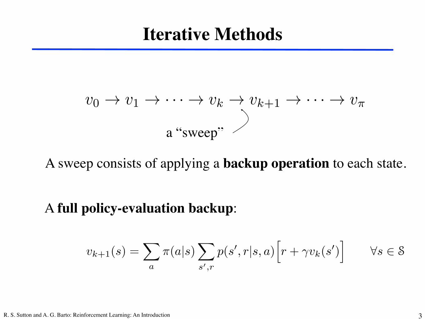
Iterative Methods
a “sweep”
A sweep consists of applying a backup operation to each state.
A full policy-evaluation backup:
v0 ! v1 ! · · · ! vk ! vk+1 ! · · · ! v⇡
v⇡(s) =X
a
⇡(a|s)X
s0,r
p(s0, r|s, a)hr + �v⇡(s
0)
i
vk+1(s) =X
a
⇡(a|s)X
s0,r
p(s0, r|s, a)hr + �vk(s
0)
i8s 2 S
v⇡(s) = E⇡[Gt | St = s] = E⇡
" 1X
k=0
�kRt+k+1
����� St = s
#
v⇡(s) = E⇡
⇥Rt+1 + �Rt+2 + �2Rt+3 + · · ·
�� St=s⇤
= E⇡[Rt+1 + �v⇡(St+1) | St=s] (1)
=
X
a
⇡(a|s)X
s0,r
p(s0, r|s, a)hr + �v⇡(s
0)
i, (2)
v⇤(s) = max
aq⇡⇤(s, a)
= max
aE[Rt+1 + �v⇤(St+1) | St=s,At=a] (3)
= max
a
X
s0,r
p(s0, r|s, a)⇥r + �v⇤(s
0)
⇤. (4)
i
R. S. Sutton and A. G. Barto: Reinforcement Learning: An Introduction 5
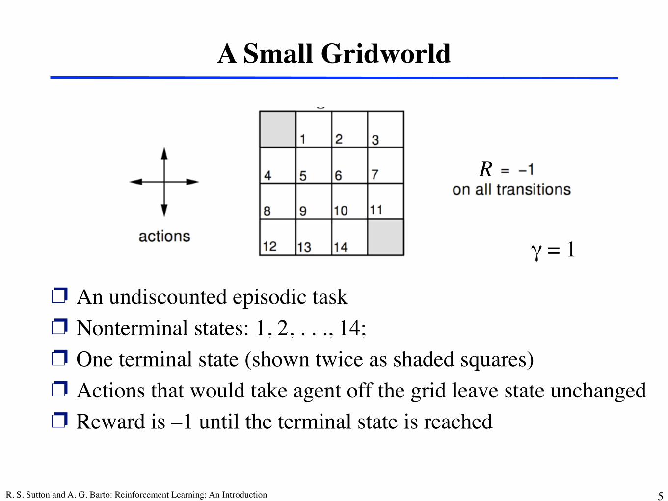
A Small Gridworld
❐ An undiscounted episodic task❐ Nonterminal states: 1, 2, . . ., 14; ❐ One terminal state (shown twice as shaded squares)❐ Actions that would take agent off the grid leave state unchanged❐ Reward is –1 until the terminal state is reached
R
γ = 1
R. S. Sutton and A. G. Barto: Reinforcement Learning: An Introduction 6
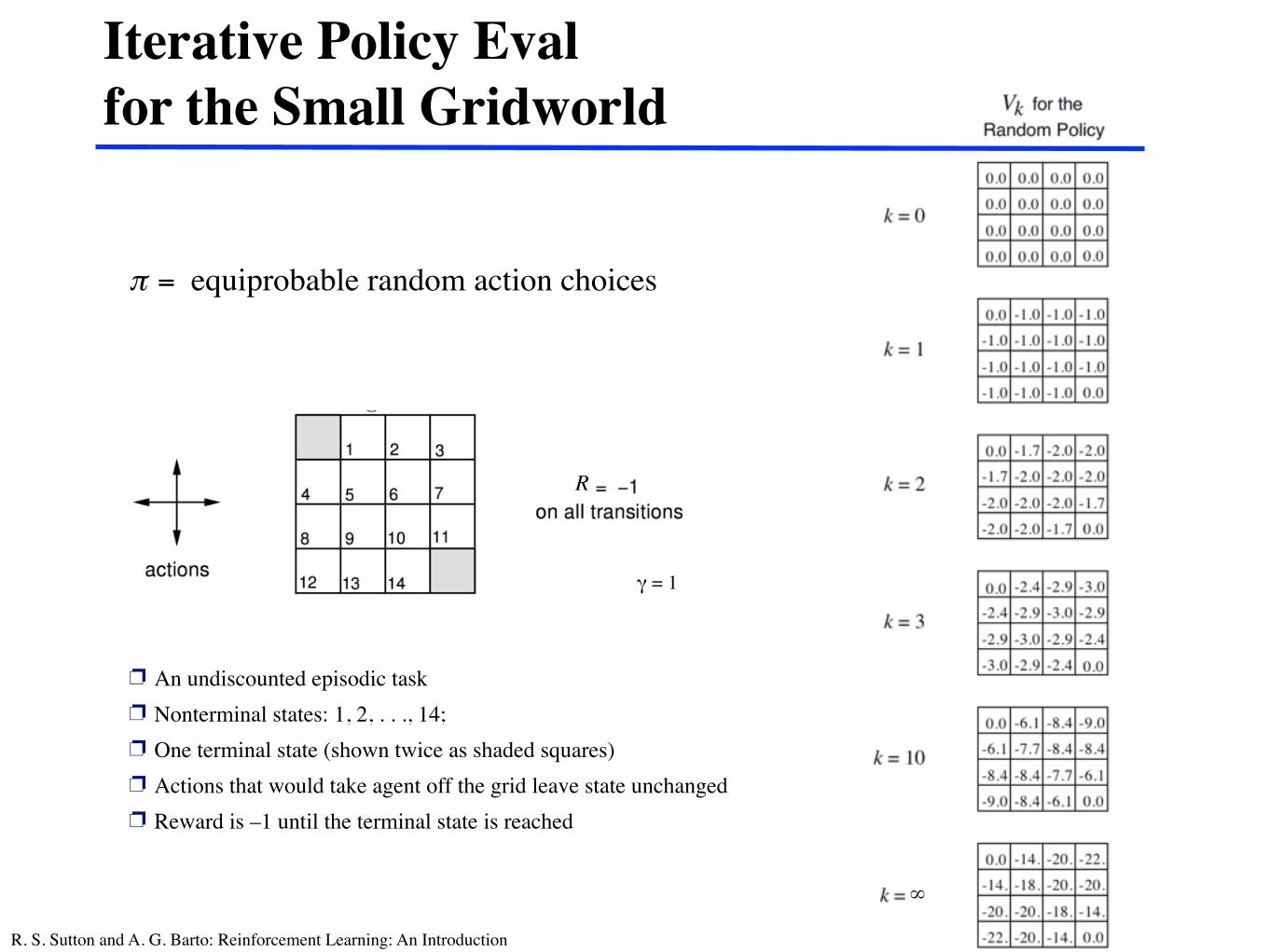
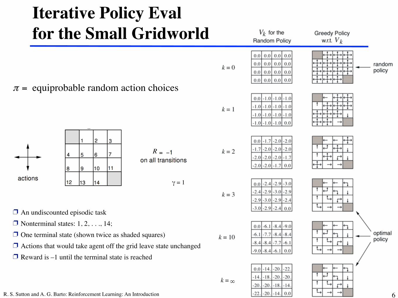
Iterative Policy Eval for the Small Gridworld
€
π = equiprobable random action choices
∞
R
γ = 1
❐ An undiscounted episodic task❐ Nonterminal states: 1, 2, . . ., 14; ❐ One terminal state (shown twice as shaded squares)❐ Actions that would take agent off the grid leave state unchanged❐ Reward is –1 until the terminal state is reached
R. S. Sutton and A. G. Barto: Reinforcement Learning: An Introduction 4
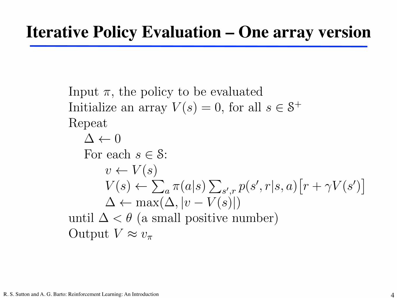
Iterative Policy Evaluation – One array version86 CHAPTER 4. DYNAMIC PROGRAMMING
Input ⇡, the policy to be evaluatedInitialize an array V (s) = 0, for all s 2 S+
Repeat� 0For each s 2 S:
v V (s)V (s)
Pa ⇡(a|s)
Ps0,r p(s0, r|s, a)
⇥r + �V (s0)
⇤
� max(�, |v � V (s)|)until � < ✓ (a small positive number)Output V ⇡ v⇡
Figure 4.1: Iterative policy evaluation.
Another implementation point concerns the termination of the algorithm.Formally, iterative policy evaluation converges only in the limit, but in practiceit must be halted short of this. A typical stopping condition for iterative policyevaluation is to test the quantity maxs2S |vk+1(s)�vk(s)| after each sweep andstop when it is su�ciently small. Figure 4.1 gives a complete algorithm foriterative policy evaluation with this stopping criterion.
Example 4.1 Consider the 4⇥4 gridworld shown below.
actions
r = !1
on all transitions
1 2 3
4 5 6 7
8 9 10 11
12 13 14
R
The nonterminal states are S = {1, 2, . . . , 14}. There are four actions pos-sible in each state, A = {up, down, right, left}, which deterministicallycause the corresponding state transitions, except that actions that would takethe agent o↵ the grid in fact leave the state unchanged. Thus, for instance,p(6|5, right) = 1, p(10|5, right) = 0, and p(7|7, right) = 1. This is an undis-counted, episodic task. The reward is �1 on all transitions until the terminalstate is reached. The terminal state is shaded in the figure (although it isshown in two places, it is formally one state). The expected reward function isthus r(s, a, s0) = �1 for all states s, s0 and actions a. Suppose the agent followsthe equiprobable random policy (all actions equally likely). The left side ofFigure 4.2 shows the sequence of value functions {vk} computed by iterativepolicy evaluation. The final estimate is in fact v⇡, which in this case gives foreach state the negation of the expected number of steps from that state until
R. S. Sutton and A. G. Barto: Reinforcement Learning: An Introduction 6
Iterative Policy Eval for the Small Gridworld
∞
❐ An undiscounted episodic task❐ Nonterminal states: 1, 2, . . ., 14; ❐ One terminal state (shown twice as shaded squares)❐ Actions that would take agent off the grid leave state unchanged❐ Reward is –1 until the terminal state is reached
€
π = equiprobable random action choices
R
γ = 1
R. S. Sutton and A. G. Barto: Reinforcement Learning: An Introduction 17
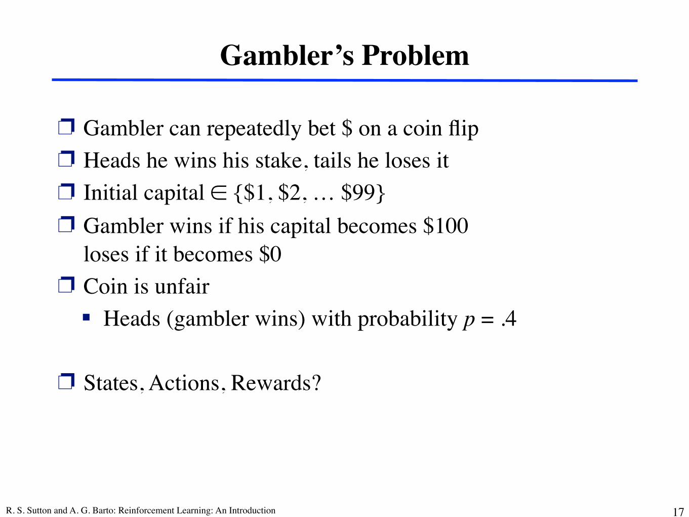
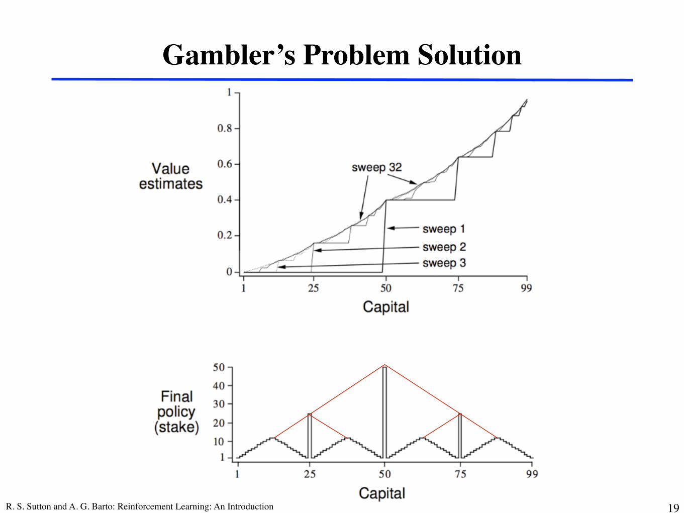
Gambler’s Problem
❐ Gambler can repeatedly bet $ on a coin flip❐ Heads he wins his stake, tails he loses it❐ Initial capital ∈ {$1, $2, … $99}❐ Gambler wins if his capital becomes $100
loses if it becomes $0❐ Coin is unfair
! Heads (gambler wins) with probability p = .4
❐ States, Actions, Rewards?
R. S. Sutton and A. G. Barto: Reinforcement Learning: An Introduction 18
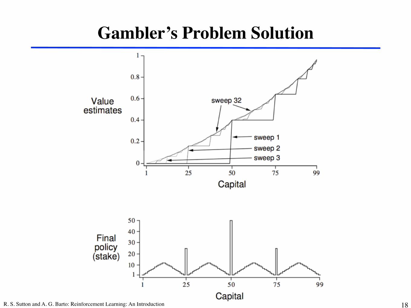
Gambler’s Problem Solution
R. S. Sutton and A. G. Barto: Reinforcement Learning: An Introduction 19
Gambler’s Problem Solution
R. S. Sutton and A. G. Barto: Reinforcement Learning: An Introduction 22
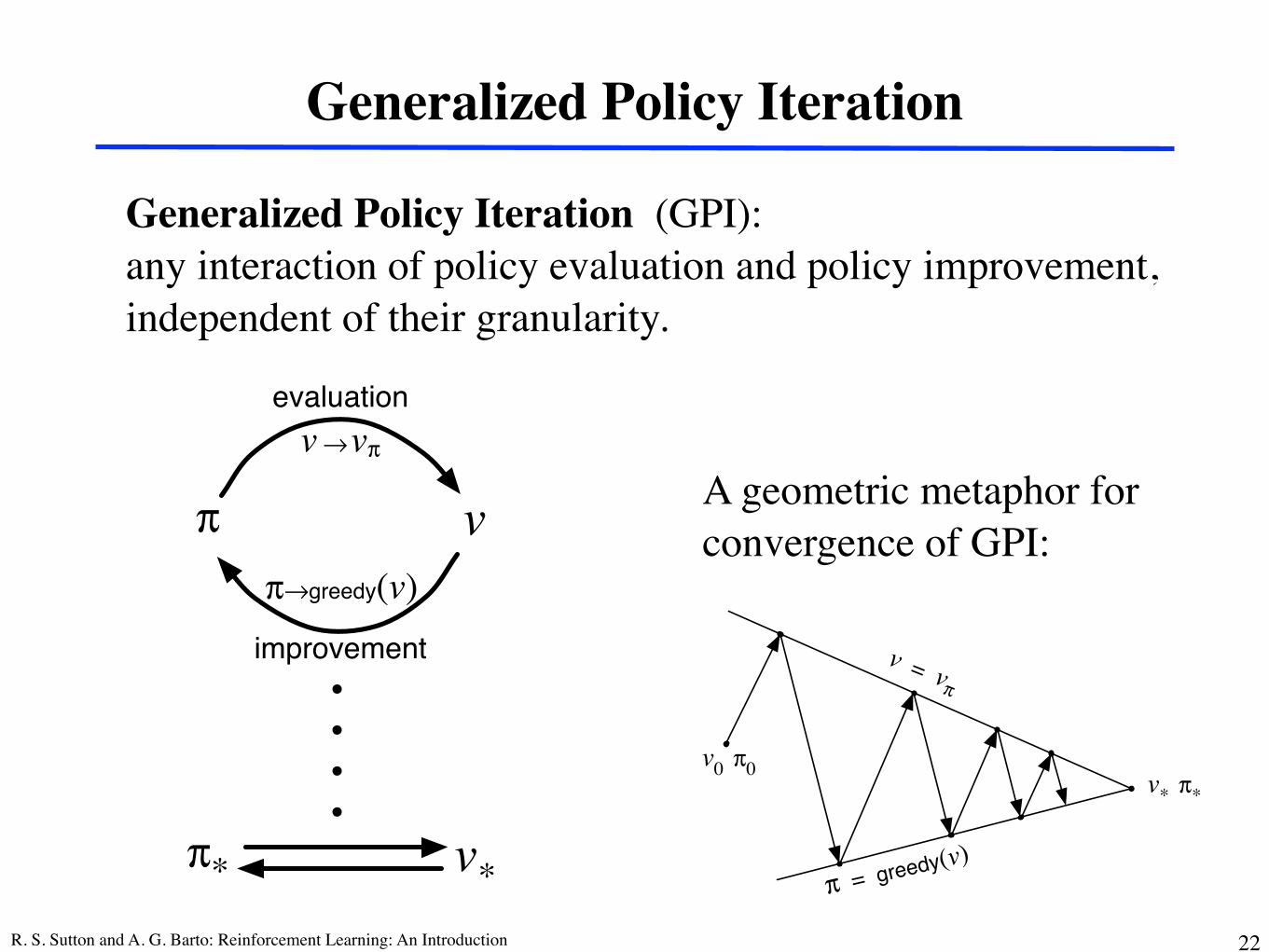
Generalized Policy Iteration
Generalized Policy Iteration (GPI): any interaction of policy evaluation and policy improvement, independent of their granularity.
A geometric metaphor forconvergence of GPI:
100 CHAPTER 4. DYNAMIC PROGRAMMING
π v
evaluationv → vπ
improvement
π→greedy(v)
v*π*
Figure 4.7: Generalized policy iteration: Value and policy functions interactuntil they are optimal and thus consistent with each other.
being driven toward the value function for the policy. This overall schema forGPI is illustrated in Figure 4.7.
It is easy to see that if both the evaluation process and the improvementprocess stabilize, that is, no longer produce changes, then the value functionand policy must be optimal. The value function stabilizes only when it is con-sistent with the current policy, and the policy stabilizes only when it is greedywith respect to the current value function. Thus, both processes stabilize onlywhen a policy has been found that is greedy with respect to its own evaluationfunction. This implies that the Bellman optimality equation (4.1) holds, andthus that the policy and the value function are optimal.
The evaluation and improvement processes in GPI can be viewed as bothcompeting and cooperating. They compete in the sense that they pull in op-posing directions. Making the policy greedy with respect to the value functiontypically makes the value function incorrect for the changed policy, and mak-ing the value function consistent with the policy typically causes that policy nolonger to be greedy. In the long run, however, these two processes interact tofind a single joint solution: the optimal value function and an optimal policy.
One might also think of the interaction between the evaluation and im-provement processes in GPI in terms of two constraints or goals—for example,as two lines in two-dimensional space:
4.7. EFFICIENCY OF DYNAMIC PROGRAMMING 101
v0 π0
v = vπ
π = greedy(v)
v* π*
Although the real geometry is much more complicated than this, the diagramsuggests what happens in the real case. Each process drives the value functionor policy toward one of the lines representing a solution to one of the twogoals. The goals interact because the two lines are not orthogonal. Drivingdirectly toward one goal causes some movement away from the other goal.Inevitably, however, the joint process is brought closer to the overall goal ofoptimality. The arrows in this diagram correspond to the behavior of policyiteration in that each takes the system all the way to achieving one of the twogoals completely. In GPI one could also take smaller, incomplete steps towardeach goal. In either case, the two processes together achieve the overall goalof optimality even though neither is attempting to achieve it directly.
4.7 E�ciency of Dynamic Programming
DP may not be practical for very large problems, but compared with othermethods for solving MDPs, DP methods are actually quite e�cient. If weignore a few technical details, then the (worst case) time DP methods take tofind an optimal policy is polynomial in the number of states and actions. If n
and m denote the number of states and actions, this means that a DP methodtakes a number of computational operations that is less than some polynomialfunction of n and m. A DP method is guaranteed to find an optimal policy inpolynomial time even though the total number of (deterministic) policies is m
n.In this sense, DP is exponentially faster than any direct search in policy spacecould be, because direct search would have to exhaustively examine each policyto provide the same guarantee. Linear programming methods can also be usedto solve MDPs, and in some cases their worst-case convergence guarantees arebetter than those of DP methods. But linear programming methods becomeimpractical at a much smaller number of states than do DP methods (by afactor of about 100). For the largest problems, only DP methods are feasible.
DP is sometimes thought to be of limited applicability because of the curse
R. S. Sutton and A. G. Barto: Reinforcement Learning: An Introduction 12
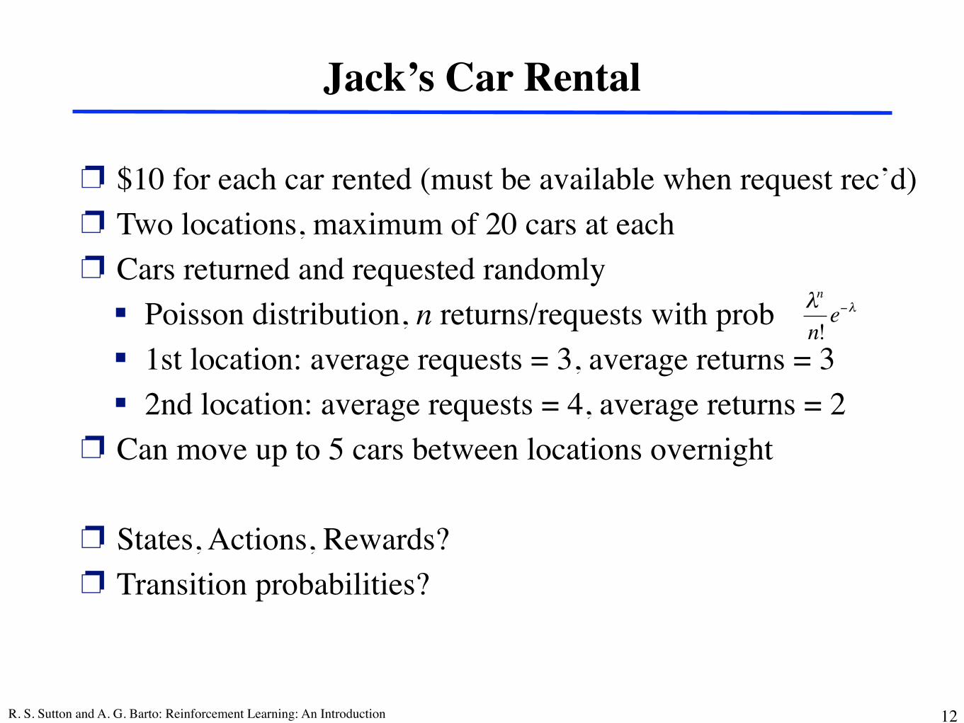
Jack’s Car Rental
❐ $10 for each car rented (must be available when request rec’d)❐ Two locations, maximum of 20 cars at each❐ Cars returned and requested randomly
! Poisson distribution, n returns/requests with prob! 1st location: average requests = 3, average returns = 3! 2nd location: average requests = 4, average returns = 2
❐ Can move up to 5 cars between locations overnight
❐ States, Actions, Rewards?❐ Transition probabilities?
€
λn
n!e−λ
R. S. Sutton and A. G. Barto: Reinforcement Learning: An Introduction 13
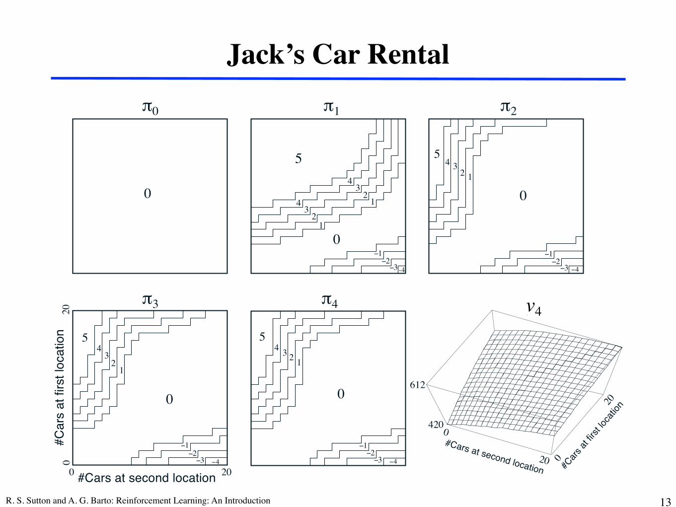
Jack’s Car Rental
94 CHAPTER 4. DYNAMIC PROGRAMMING
4V
612
#Cars at second location
0420
20 0
20
#Cars
at firs
t lo
cation
1
1
5
!1!2
-4
432
432
!3
0
0
5
!1!2!3 !4
12
34
0
"1"0 "2
!3 !4
!2
0
12
34
!1
"3
2
!4!3!2
0
1
34
5
!1
"4
#Cars at second location
#C
ars
at
firs
t lo
ca
tio
n
5
200
020 v4
Figure 4.4: The sequence of policies found by policy iteration on Jack’s carrental problem, and the final state-value function. The first five diagrams show,for each number of cars at each location at the end of the day, the numberof cars to be moved from the first location to the second (negative numbersindicate transfers from the second location to the first). Each successive policyis a strict improvement over the previous policy, and the last policy is optimal.
R. S. Sutton and A. G. Barto: Reinforcement Learning: An Introduction 31
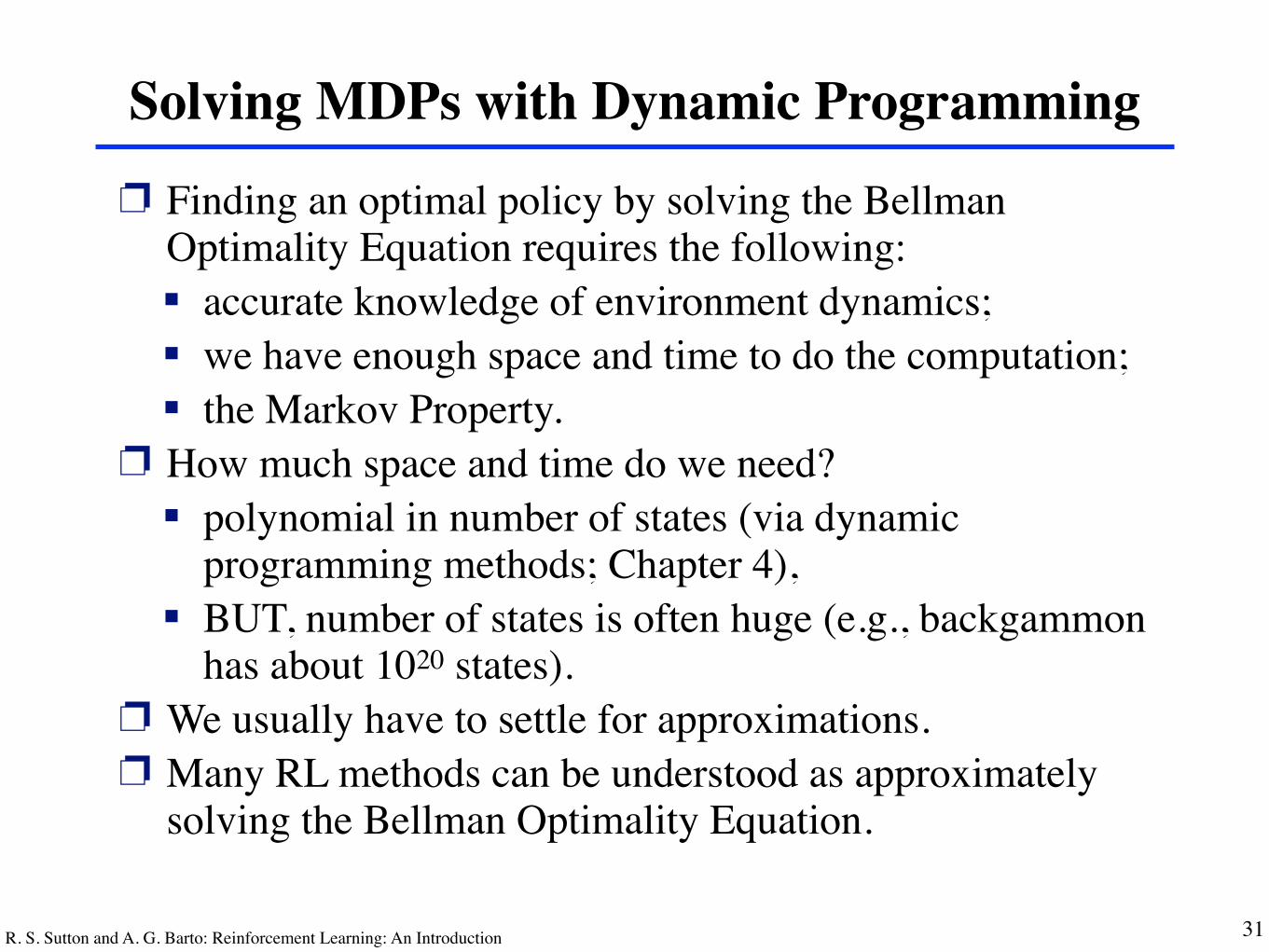
Solving MDPs with Dynamic Programming❐ Finding an optimal policy by solving the Bellman
Optimality Equation requires the following:! accurate knowledge of environment dynamics;! we have enough space and time to do the computation;! the Markov Property.
❐ How much space and time do we need?! polynomial in number of states (via dynamic
programming methods; Chapter 4),! BUT, number of states is often huge (e.g., backgammon
has about 1020 states).❐ We usually have to settle for approximations.❐ Many RL methods can be understood as approximately
solving the Bellman Optimality Equation.
R. S. Sutton and A. G. Barto: Reinforcement Learning: An Introduction 23
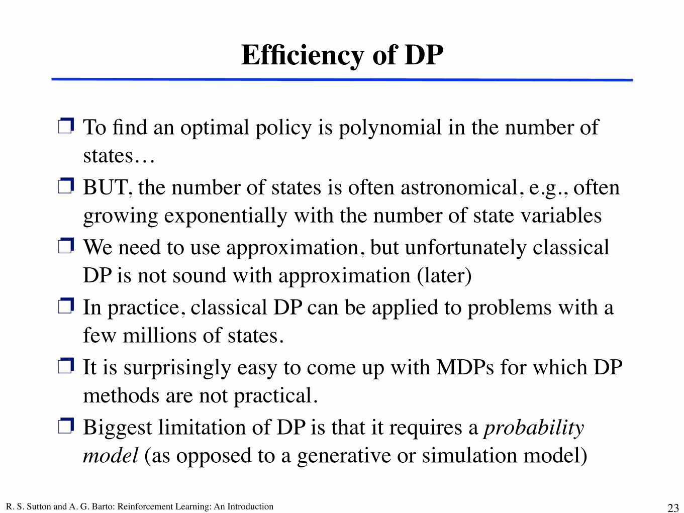
Efficiency of DP
❐ To find an optimal policy is polynomial in the number of states…
❐ BUT, the number of states is often astronomical, e.g., often growing exponentially with the number of state variables
❐ We need to use approximation, but unfortunately classical DP is not sound with approximation (later)
❐ In practice, classical DP can be applied to problems with a few millions of states.
❐ It is surprisingly easy to come up with MDPs for which DP methods are not practical.
❐ Biggest limitation of DP is that it requires a probability model (as opposed to a generative or simulation model)
R. S. Sutton and A. G. Barto: Reinforcement Learning: An Introduction
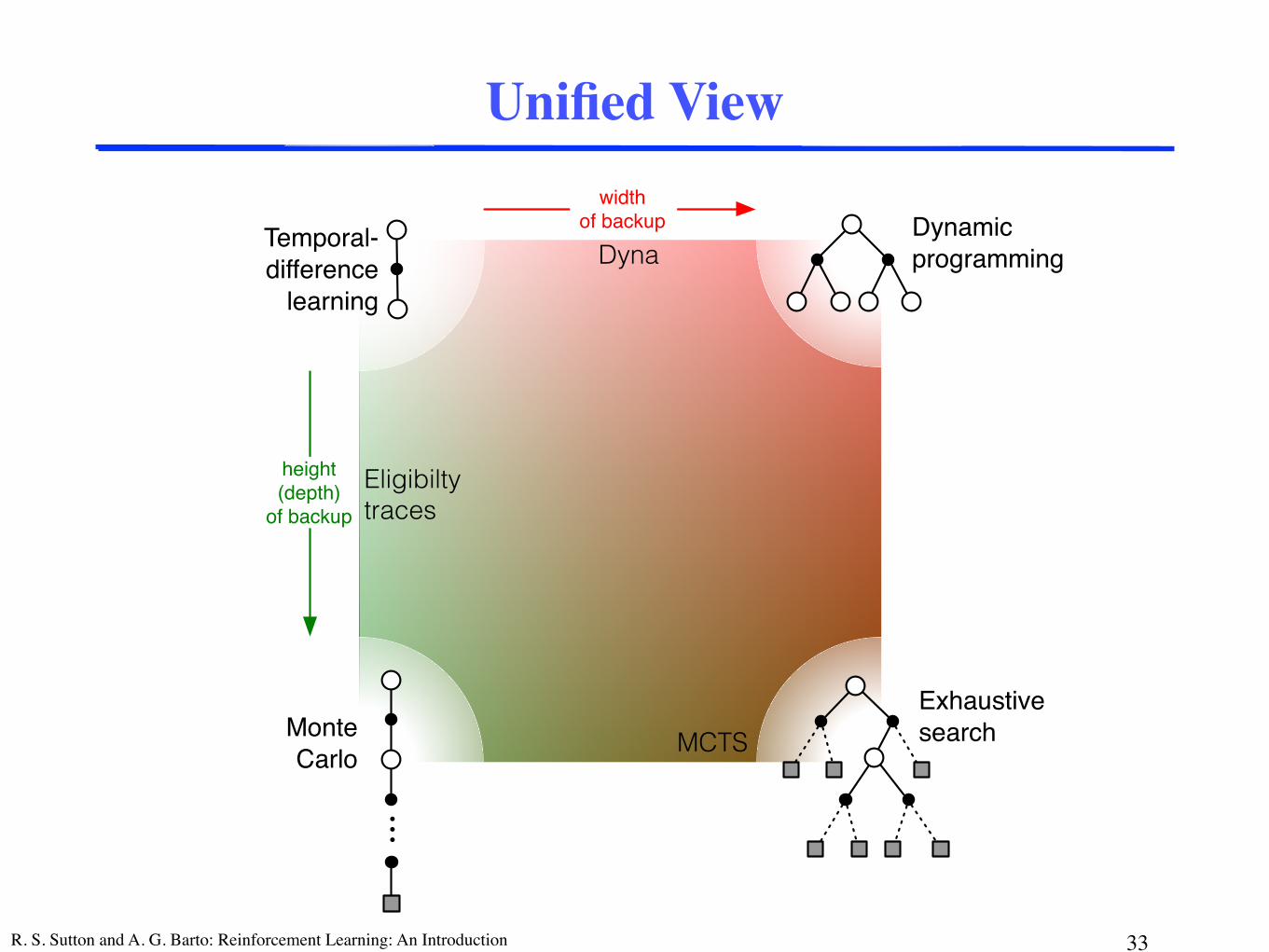
widthof backup
height(depth)
of backup
Temporal-difference
learning
Dynamicprogramming
MonteCarlo
...
Exhaustivesearch
33
Unified View
Eligibilty traces
Dyna
MCTS
Related Documents