Belief Aggregation with Automated Market Makers * Rajiv Sethi † Jennifer Wortman Vaughan ‡ July 10, 2013 Abstract We consider the properties of a cost function based automated market maker aggregating the beliefs of risk-averse traders with finite budgets. Individuals can interact with the market maker an arbitrary number of times before the state of the world is revealed. We show that the resulting sequence of prices offered by the market maker is convergent under general conditions, and explore the properties of the limiting price and trader portfolios. The limiting price cannot be expressed as a function of trader beliefs, since it is sensitive to the market maker’s cost function as well as the order in which traders interact with the market. For a range of trader preferences, however, we show numerically that the limiting price provides a good approximation to a weighted average of beliefs, inclusive of the market designer’s prior belief as reflected in the initial contract price. This average is computed by weighting trader beliefs by their respective budgets, and weighting the initial contract price by the market maker’s worst-case loss, implicit in the cost function. Since cost function parameters are chosen by the market designer, this allows for an inference regarding the budget-weighted average of trader beliefs. * This project was initiated while Sethi was visiting Microsoft Research, New York City. † Department of Economics, Barnard College, Columbia University and the Santa Fe Institute. ‡ Microsoft Research, New York City and UCLA.

Welcome message from author
This document is posted to help you gain knowledge. Please leave a comment to let me know what you think about it! Share it to your friends and learn new things together.
Transcript
Belief Aggregation with Automated Market Makers∗
Rajiv Sethi† Jennifer Wortman Vaughan‡
July 10, 2013
Abstract
We consider the properties of a cost function based automated market maker aggregating the
beliefs of risk-averse traders with finite budgets. Individuals can interact with the market
maker an arbitrary number of times before the state of the world is revealed. We show that the
resulting sequence of prices offered by the market maker is convergent under general conditions,
and explore the properties of the limiting price and trader portfolios. The limiting price cannot
be expressed as a function of trader beliefs, since it is sensitive to the market maker’s cost
function as well as the order in which traders interact with the market. For a range of trader
preferences, however, we show numerically that the limiting price provides a good approximation
to a weighted average of beliefs, inclusive of the market designer’s prior belief as reflected in the
initial contract price. This average is computed by weighting trader beliefs by their respective
budgets, and weighting the initial contract price by the market maker’s worst-case loss, implicit
in the cost function. Since cost function parameters are chosen by the market designer, this
allows for an inference regarding the budget-weighted average of trader beliefs.
∗This project was initiated while Sethi was visiting Microsoft Research, New York City.†Department of Economics, Barnard College, Columbia University and the Santa Fe Institute.‡Microsoft Research, New York City and UCLA.
1 Introduction
It has long been recognized that markets are mechanisms that accomplish both resource allocation
and belief aggregation, and that these two functions are inextricably linked.1 In many instances
where belief aggregation is desirable, however, spontaneous markets do not exist. This is the case
within organizations, where mechanisms such as meetings and internal correspondence are highly
imperfect vehicles for the transmission of information and opinion.2
The need for belief aggregation and the inefficiency of traditional mechanisms for securing it
has led a number of organizations to experiment with internal “prediction markets” that involve
the purchase and sale of securities with state-contingent payoffs. Among the earliest adopters
were Hewlett-Packard, using real money contracts, and Google, which created an internal currency
convertible into raffle tickets and prizes (Chen and Plott, 2002; Cowgill et al., 2009). Several
other organizations have since followed suit, including non-profits and government agencies.3 The
Penn-Berkeley Good Judgment Project, twice winners of a forecasting competition sponsored by
IARPA (the U.S. Intelligence Advanced Research Projects Activity), has also made extensive use
of prediction markets (Ungar et al., 2012).
The earliest prediction markets, including those used by HP and Google, were web-based dou-
ble auctions for the trading of binary securities. Their design was based on the pioneering Iowa
Electronic Markets, which has listed contracts on such events as the outcomes of presidential and
congressional elections for over two decades (Berg et al., 2008). This is a peer-to-peer market in
which the exchange itself bears no risk, and traders are required to have enough cash margin to
cover their worst case loss at all times. Such markets can work well if there is active participation
by a large number of traders and sufficient liquidity to maintain interest. But since all liquidity
is endogenously generated by the market participants, there may be situations in which bid-ask
spreads remain wide and trading is intermittent for long stretches of time. Furthermore, prices
across different contracts may be inconsistent in the sense that opportunities for arbitrage remain
unexploited.4
An alternative approach to prediction market construction entails the use of an automated
1See, especially, Hayek (1945), who drew attention to the importance of the latter role.2Chen and Plott (2002) make this point as follows: “Gathering the bits and pieces by traditional means, such
as business meetings, is highly inefficient because of a host of practical problems related to location, incentives,
the insignificant amounts of information in any one place, and even the absence of a methodology for gathering it.
Furthermore, business practices such a quotas and budget settings create incentives for individuals not to reveal their
information.”3Among corporations, the list includes Microsoft, Intel, Eli Lily, GE, Siemens, and many others (Charette, 2007;
Broughton, 2013). Providers of software for the implementation of prediction markets include Inkling, Consensus
Point, and Lumenogic.4Chen and Plott (2002), for instance, report that the sum of the market prices of a set of binary securities on
mutually exclusive and exhaustive events exceeded the amount that the single winning security would pay off in all
12 experiments in the HP market.
2

market maker that stands ready to buy and sell an indefinite amount of any contract, but adjusts
prices in response to its net position. The most commonly studied class of such markets is that of
market scoring rules, of which the logarithmic market scoring rule is an example (Hanson, 2003,
2007; Chen and Pennock, 2007). These market makers, which are based on proper scoring rules,
maintain a bid-ask spread that is identically zero at all times, but only an infinitesimal amount
can be purchased or sold at the currently quoted price. The average price at which an order
trades depends on order size in accordance with a specified potential function referred to as the
cost function. Market scoring rules satisfy several nice properties. Arbitrage opportunities are
prevented from arising, so that no trader may ever make a single purchase or sale in a way that
guarantees a positive net payoff regardless of the state of the world. Additionally and crucially,
the overall exposure to loss faced by the market maker is kept bounded.5 The prediction market
platforms offered by Consensus Point and Inkling are based on automated market makers of this
kind.
In this paper we focus on the properties of an algorithmic prediction market in which binary
securities are traded by myopic, risk-averse individuals with heterogeneous prior beliefs and finite
budgets. Traders interact repeatedly with a market maker rather than directly with each other,
and can buy and sell unlimited amounts (subject to budget and collateral constraints) at prices
determined by the market maker’s cost function. A sequence of prices is generated by the behavior
of traders, who can adjust their portfolios each time they face the market. We show that this price
sequence is convergent under very general conditions. Convergence does not follow from feasibility
alone, even in a market with a single trader, since any such trader can move the price back and
forth between two points without ever exhausting her budget. Hence convergence relies on the
optimality of trader behavior.
Given convergence, we turn to the question of how the limiting price and trader portfolios
should be interpreted. The beliefs of individual traders cannot be inferred from their respective
limiting portfolios even in an ordinal sense. For instance, it is is possible for a trader with more
pessimistic beliefs about the likelihood of an event to end up with larger asset position than one
with the same initial budget and more optimistic beliefs. This can happen, for instance, because
the former faced lower prices on average when accessing the market in early periods. Hence the
ranking of trader beliefs need not correspond to the ranking of asset positions even if all initial
budgets are identical.6 Given the limiting price, however, the set of traders with positive limiting
asset positions must be more optimistic about the likelihood of the event than the belief implicit
in this price, while those with negative limiting asset positions must be more pessimistic.
5Abernethy et al. (2011, 2013) have generalized the idea of a market scoring rule to settings in which the state
space is exponentially large compared with the set of offered securities, and fully characterized the class of automated
market makers that guarantee no arbitrage, bounded market maker loss, and other desirable properties. Chen et al.
(2013) have extended these results to cover markets over continuous state spaces.6This is a common feature in markets where out-of-equilibrium trading can occur; see, for instance, Hahn and
Negishi (1962) and Foley (1994).
3
This limiting price clearly cannot be expressed as a function of trader beliefs, since it is sensitive
to the market maker cost function as well as the order in which traders interact with the market.
We show that for a range of beliefs and trader preferences, the limiting price provides a good
approximation to a weighted average of beliefs, where trader beliefs are weighted by their budgets,
the price faced by the initial trader is interpreted as the market maker’s belief, and this belief is
weighted by the market maker’s maximum loss implicit in the cost function. Since the cost function
parameters are chosen by the market designer, this approximation allows for an inference regarding
the budget-weighted average of trader beliefs. Furthermore, in markets with internal currencies,
the budgets themselves can be chosen to be equal if one wants to estimate a simple average of
trader beliefs. Alternatively, budgets can be allowed to vary endogenously by allowing the same
currency to be used in a sequence of markets, so that traders with strong forecasting performance
come to carry greater weight over time.
There are two strands of literature to which our work is directly connected. Pennock (1999),
Manski (2006), Gjerstad (2004), and Wolfers and Zitzewitz (2006) have previously considered pre-
diction markets with heterogeneous priors and finite budgets, but rather than a market maker al-
lowing for a sequence of trades, they considered a single equilibrium price determined by a market
clearing condition. Manski showed that with risk-neutral traders the equilibrium price corresponds
to the corresponding quantile of the belief distribution, and can therefore be quite distant from
the average belief. When traders are risk averse with log utility, however, the equilibrium price
is precisely equal to the budget-weighted average of trader beliefs (Pennock, 1999). This con-
nection becomes approximate if one allows for departures from log utility while maintaining risk
aversion (Gjerstad, 2004; Wolfers and Zitzewitz, 2006).
A second strand of literature examines market scoring rules with a common prior but hetero-
geneous information. Ostrovsky (2012) finds that with risk-neutral traders in this setting, prices
converge to the common belief that would arise if all information were pooled and applied to the
common prior. Chen et al. (2012) showed how this idea can be used to design sets of securities to
aggregate information relevant to a particular event of interest. Full information aggregation and a
common posterior belief also occur with risk-averse traders under a weak smoothness condition (Iyer
et al., 2010). These results reflect the fact that with a common prior, posterior beliefs must be iden-
tical if they are public information (Aumann, 1976), and repeated belief announcements generically
leads to belief convergence (Geanakopolos and Polemarchakis, 1982). With heterogeneous priors,
of course, posterior beliefs may differ even if all information is aggregated. More importantly, all
information may not be aggregated if the priors themselves are unobservable (Sethi and Yildiz,
2012). In order to focus on the role of heterogeneous priors, we abstract here from differences in
information, effectively assuming that all information is public at the start of the trading process.
The market therefore serves to aggregate opinions based on the differential interpretation of public
information, rather than to aggregate information held by otherwise identical individuals with a
common prior.
4

Also related to our work is that of Othman and Sandholm (2010), who examine the prices that
emerge when a set of risk neutral traders with heterogeneous priors face an automated marker
maker in sequence, with each trader interacting with the market just once. They establish that
the last price in the resulting finite sequence is heavily dependent on the order in which traders
arrive, but that the price is relatively stable when the number of traders is large and their order
is chosen uniformly at random. In contrast, the set of traders in our model each face the market
repeatedly, resulting in an infinite sequence of prices and portfolios with a well defined limit. It is
the properties of this limit with which we are concerned.
2 The Model
We explore a setting in which a finite set of traders with heterogeneous prior beliefs and common
information interact repeatedly with an electronic market maker. When given an opportunity to
trade, each individual adjusts his market position in order to maximize expected utility conditional
on his subjective belief. This shifts the market state and determines the price faced by the next
trader, and so on, in sequence, for an indefinite number of periods.
Formally, let N = {1, ..., n} denote the set of traders. The true state of the world is denoted
ω ∈ {0, 1}, to be revealed after the trading process has run its course.7 The subjective belief of
trader i that ω = 1 is denoted pi, and each trader is endowed at the start of the process with a
cash endowment yi. Traders may have heterogeneous initial cash holdings as well as heterogeneous
beliefs.
Traders participate in a cost function based market operated by an automated market maker.
The market maker offers only a single security that may be redeemed for $1 if ω = 1 and $0
otherwise. Traders may buy or (short) sell this security, and are allowed to buy/sell arbitrary
fractions of securities. They interact with the market one at a time, repeatedly, in arbitrary order.
Specifically, let k : N → N denote the trading order, where k(t) is the trader who accesses the
market in period t. We assume that each trader can access the market an infinite number of times:
Assumption 1. For each i ∈ N , the set {t | k(t) = i} is infinite.
A special case of this arises if traders access the market in the same order repeatedly, so that
k(1), ..., k(n) are all distinct and k(t) = k(t− n) for all t > n.
At the end of any given period t ∈ N, each trader has a cash position yi,t and a (possibly
negative) asset position zi,t. Traders are constrained to take positions that leave them with non-
negative wealth in all states:
7To accommodate an unbounded number of trades one could assume, as in Ostrovsky (2012), that the sth trade
occurs at time 1 − 1/s and that the state is revealed at time 1. In practice, convergence to a limiting price is quite
rapid and requires just a few rounds of trading.
5
Assumption 2. For each i and t, yi,t ≥ 0 and yi,t + zi,t ≥ 0.
For traders with positive asset positions this means only that their cash cannot be negative. For
traders with short positions, it means that they must have enough cash collateral to meet their
obligations if ω = 1 occurs. Initially all asset positions are zero and cash positions are strictly
positive: zi,0 = 0 and yi,0 = yi > 0 for all i.
The behavior of the market maker is fully specified by a potential function C, referred to as the
cost function. Let qt denote the (possibly negative) number of securities that have been purchased
from the market at the end of period t, and set q0 = 0. If trader k(t) purchases rt units of the
security in period t, he is charged C(qt) − C(qt−1), where qt = qt−1 + rt. Specifically, if rt is the
(possibly negative) quantity of the security purchased by the trader j = k(t) in period t, then
zj,t = zj,t−1 + rt
and
yj,t = yj,t−1 − C(qt) + C(qt−1).
The use of a cost function implies that the market is path independent in the sense that the cost of
purchasing r units of the security and then immediately purchasing r′ units is the same as the cost
of purchasing r+ r′ units together in a single purchase. The cost function C satisfies the following
standard properties (Abernethy et al., 2011, 2013).
Assumption 3. C : R→ R is smooth, increasing, convex, and satisfies bounded loss.
The bounded loss condition requires that regardless of trader budgets, behavior and the realized
state, there is a finite bound on the loss that the market maker can suffer. Specifically, the quantity
maxq∈R{max {q − C(q),−C(q)}}
is assumed to be upper bounded.
At the end of period t the instantaneous price πt of the security, that is, the price per unit
security of an infinitesimally small fraction of a security, is simply C ′(qt), the derivative of C
evaluated at q = qt. The bounded loss condition implies that for any π ∈ (0, 1), there exists some
q ∈ R such that C ′(q) = π (Abernethy et al., 2011, 2013). Let p0 = C ′(0) denote the initial price,
before the onset of trading. This may be interpreted as the prior belief of the market maker.
When given the opportunity to trade, traders myopically maximize the expected value of a
utility function u(w), where w is the wealth remaining after the true state has been revealed.8 We
assume the following.
8For simplicity we assume that all traders share the same utility function, but all of our theoretical results carry
over easily to the setting in which each trader i has a distinct utility function ui satisfying the criteria in Assumption 4.
6

Assumption 4. u : R+ → R is smooth, increasing and strictly concave, with limw→0 u′(w) =∞.
Hence trader j = k(t) chooses rt ∈ R to maximize
pju(zj,t + yj,t) + (1− pj)u(yj,t). (1)
Since u is increasing and concave, and C is convex, this quantity is concave in rt and it suffices to
find a local maximum.
After the period t transaction, the state is updated as follows:
yj,t ← yj,t−1 − C(qt−1 + rt) + C(qt−1)
zj,t ← zj,t−1 + rt
yi,t ← yi,t−1 ∀i 6= j
zi,t ← zi,t−1 ∀i 6= j
qt ← qt−1 + rt
πt ← C ′(qt)
The next trader to face the market, k(t+ 1), then encounters the market state qt, and so on. This
generates sequences of prices {πt}, market maker positions {qt}, and trader portfolios {yi,t, zi,t}.We show below that these sequences necessarily converge, and use bars to denote the limiting values
of all variables. Hence π denotes the limiting price, q the limiting market state, and (yi, zi) the
limiting portfolio of each trader i.
3 Examples
The model may be illustrated with some simple examples. Suppose that the trader preferences
belong to the following class:
u(w) =w1−ρ
1− ρ(2)
where ρ ≥ 0 is a parameter. This class of CRRA (Constant Relative Risk Aversion) preferences
includes risk neutrality and log utility as special cases.9
Prices are set by the market maker in accordance with a Logarithmic Market Scoring Rule
(LMSR), based on the cost function
C(q) = b log(eq/b + a) (3)
9Specifically, risk neutrality corresponds to ρ = 0 and log utility to the limit as ρ→ 1. Risk neutrality falls outside
of our model as Assumption 4 is violated.
7
0 100.45
0.73
k (1) = 2
k (1) = 1
Period
Price
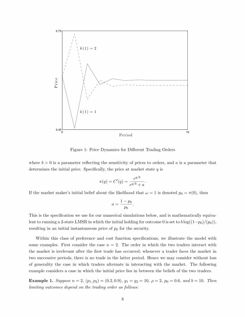
Figure 1: Price Dynamics for Different Trading Orders
where b > 0 is a parameter reflecting the sensitivity of prices to orders, and a is a parameter that
determines the initial price. Specifically, the price at market state q is
π(q) = C ′(q) =eq/b
eq/b + a.
If the market maker’s initial belief about the likelihood that ω = 1 is denoted p0 = π(0), then
a =1− p0p0
.
This is the specification we use for our numerical simulations below, and is mathematically equiva-
lent to running a 2-state LMSR in which the initial holding for outcome 0 is set to b log((1−p0)/(p0)),resulting in an initial instantaneous price of p0 for the security.
Within this class of preference and cost function specifications, we illustrate the model with
some examples. First consider the case n = 2. The order in which the two traders interact with
the market is irrelevant after the first trade has occurred; whenever a trader faces the market in
two successive periods, there is no trade in the latter period. Hence we may consider without loss
of generality the case in which traders alternate in interacting with the market. The following
example considers a case in which the initial price lies in between the beliefs of the two traders.
Example 1. Suppose n = 2, (p1, p2) = (0.2, 0.9), y1 = y2 = 10, ρ = 2, p0 = 0.6, and b = 10. Then
limiting outcomes depend on the trading order as follows:
8

0 180.35
0.7
Period
Price
Figure 2: Rebalancing by Trader 2 (transactions in bold)
k(1) π q (y1, y2) (z1, z2)
1 0.59 0.39 (14.75, 5.48) (−8.61, 8.22)
2 0.58 1.00 (15.58, 5.01) (−8.89, 7.89)
The price paths for the two cases are shown in Figure 1. Note that the order of trading affects
the limiting outcomes. This order dependence of the limiting price does not generally arise in
information-based models with a common prior, as in Ostrovsky (2012).
In Example 1, regardless of the trading order, traders always trade in the direction of their
beliefs, buying when the price is below their subjective belief and selling when it is above. But this
need not always be the case, as the following example shows.
Example 2. Suppose n = 3, (p1, p2, p3) = (0.1, 0.7, 0.9), y1 = y2 = y3 = 10, k(t) = t for t ≤ 3
and k(t) = k(t − 3) thereafter. All other specifications are as in Example 1. Then the sequence
of prices converges to π = 0.58, with limiting market maker position q = 0.79. Limiting holdings
of cash are (y1, y2, y3) = (16.21, 9.00, 5.26) and limiting holdings of the security are (z1, z2, z3) =
(−11.62, 2.68, 8.14). Trader 2 buys at time t = 2 and sells at time t = 5, although πt < p2 for all t.
Figure 2 illustrates the dynamics of prices and trades for the first 18 periods. Each of the three
participants trades six times in sequence. The initial price equals the initial market maker belief.
As can be seen from the figure, the second trader buys at t = 2 but sells at t = 5, even though the
9
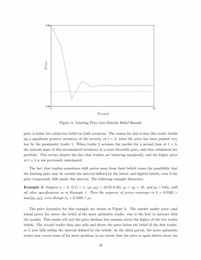
0 100.53
0.64
Period
Price
Figure 3: Limiting Price Lies Outside Belief Bounds
price is below her subjective belief on both occasions. The reason for this is that this trader builds
up a significant positive inventory of the security at t = 2, when the price has been pushed very
low by the pessimistic trader 1. When trader 2 accesses the market for a second time at t = 5,
she unloads some of this accumulated inventory at a more favorable price, and thus rebalances her
portfolio. This occurs despite the fact that traders are behaving myopically, and the higher price
at t = 5 is not previously anticipated.
The fact that traders sometimes shift prices away from their beliefs raises the possibility that
the limiting price may lie outside the interval defined by the lowest and highest beliefs, even if the
price temporarily falls inside this interval. The following example illustrates.
Example 3. Suppose n = 2, k(1) = 1, (p1, p2) = (0.55, 0.40), y1 = y2 = 10, and p0 = 0.64, with
all other specifications as in Example 1. Then the sequence of prices converges to π = 0.5582 >
max{p1, p2}, even though π2 = 0.5403 < p1.
The price dynamics for this example are shown in Figure 3. The market maker prior (and
initial price) lies above the belief of the most optimistic trader, who is the first to interact with
the market. This trader sell and the price declines but remains above the higher of the two trader
beliefs. The second trader then also sells and drives the price below the belief of the first trader,
so it now falls within the interval defined by the beliefs. In the third period, the more optimistic
trader now covers some of his short position, to an extent that the price is again driven above his
10

belief. After this point the price never falls back below the highest belief.
We show below that this phenomenon cannot occur if the market maker belief (and hence initial
price) itself lies within the interval defined by the trader beliefs. That is, if the initial price is in
the interval, then all subsequent prices also lie in this interval.
4 Price Bounds
We know that traders may trade against their beliefs: an optimist may sell at a price that is below
his expectation or a pessimist may buy at a price above his expectation. But not all such trades are
possible. The following result states that a trader will trade against his belief only if this involves
a reduction in risk, by selling from a long position or buying to cover a short position in the asset.
This is intuitive, since trading against one’s belief involves a reduction in expected payoff and can
only be motivated by a reduction in risk.10
Lemma 1. Let i = k(t).
1. If pi ≤ πt−1 and zi,t−1 ≥ 0, then πt ≤ πt−1.
2. If pi ≥ πt−1 and zi,t−1 ≤ 0, then πt ≥ πt−1.
Next we show that a trader with a positive asset position, facing a price that is below his belief,
will not buy so much of the asset that the price rises above his belief. Similarly, a trader who holds
a short position and faces a price above his belief will not sell additional units to such a degree
that the price falls below his belief.
Lemma 2. Let i = k(t).
1. If pi ≥ πt−1 and zi,t−1 ≥ 0, then πt ≤ pi.
2. If pi ≤ πt−1 and zi,t−1 ≤ 0, then πt ≥ pi.
These results allow us to place bounds on the sequence of prices. We can still show that the
price remains within the interval defined by the lowest and highest belief, as long as the initial
price lies in this interval. Define I = [pmin, pmax], where pmin and pmax are the lowest and highest
elements in the set {p0, . . . , pn}. Notice that this set includes the initial market price p0, which can
be interpreted as the belief of the market maker. We then have:
Proposition 1. For all t ≥ 0, πt ∈ I.
10Proofs of all formal claims are in the Appendix.
11

Proposition 1 establishes that prices remain within the interval defined by trader beliefs as
long as the initial price, reflecting the market designer’s prior belief, also lies in this interval and,
more generally, that the price sequence must lie in the interval defined by the entire set of beliefs,
inclusive of the market maker’s prior. An immediate implication of this is that prices are always
bounded away from the extremes of 0 and 1. We show next that the price sequence is not just
bounded in this manner but also convergent.
5 Convergence
Given that i = k(t) is the trader facing the market in period t, let s(t) denote the last period in
which this trader interacted with the market, and set s = 0 is there is no such period (that is, if i
has not traded prior to period t). If s(t) > 0, then the trader’s position (yi,t−1, zi,t−1) at the start
of period t must have been optimal at the price πs(t) at which this trader last left the market. The
following result states that this trader’s period t transaction results in a price πt that is a weighted
average of the price at which the trader last left the market, and the price at which he now finds
it.
Lemma 3. For each t such that s(t) > 0, there exists αt ∈ [0, 1) such that πt = αtπs(t)+(1−αt)πt−1.
If the prices πt−1 and πs(t) are identical, then Lemma 3 holds for any α ∈ [0, 1). If not, then the
following result establishes that there is an upper bound α < 1 such that αt < α for all t provided
that the prices πs and πt−1 are separated by some number η > 0.
Lemma 4. For any η > 0, there exists α(η) < 1 such that, for all t with s(t) > 0 and |πs−πt−1| ≥ η,
αt < α.
We are now in a position to establish convergence. We do so for the special case in which traders
interact with the market in the same fixed sequence with k(t) = k(t − n) for all t > n, although
the proof may be generalized to cover arbitrary trading orders.
For t > n define πt and πt as follows:
πt = max{πt−s | s = 0, ..., n− 1},
πt = min{πt−s | s = 0, ..., n− 1}
These are the highest and lowest prices observed over the past n periods, once the period t
transaction has been completed. Then from Lemma 3 we have:
Lemma 5. The sequences {πt} and {πt} are non-increasing and non-decreasing respectively.
12

An immediate consequence is that both sequences are convergent; let π and π denote their
respective limits. We therefore have
lim supπt = π ≥ π = lim inf πt.
The sequence of prices is convergent if and only if the above holds with strict equality. The following
is a key step in establishing convergence.
Lemma 6. For any γ > 0, there exists δ ∈ (0, γ) and t′ ∈ N such that, for all t > t′, πt > π − δimplies πt−1 > π − γ.
This result can be used to construct a sequence of n consecutive prices all of which are arbitrarily
close to π, and hence all greater than π if π < π. But every sequence of n consecutive prices must
include at least one that is no greater than π, which is enough to prove convergence:
Theorem 1. The sequence {πt} is convergent.
We now turn to the question of how the limiting price and portfolios may be interpreted, having
established that these limits are well-defined.
6 Limiting Portfolios
Recall that π denotes the limiting price. For any trader i with belief pi and limiting portfolio
(yi, zi), the following must hold:
Proposition 2. For each trader i, zi > 0 (resp. zi < 0) if and only if pi > π (resp. pi < π).
This result is very intuitive. If a trader with belief higher than the terminal price holds a short
position, such a trader could reduce risk and increase expected return by buying a small quantity
of the asset. If, instead, he holds a zero position he could increase utility despite increasing risk by
buying a small amount of the asset. Hence such a trader must hold a positive position. The case
of traders with negative positions is analogous. Note that the result does not imply that positions
are monotonic in beliefs: this need not be the case even if all budgets are equal.
Proposition 2 implies that, given the limiting price, the set of traders may be partitioned into
two groups, such that all members of one group hold positive limiting asset positions and assign
greater likelihood to the occurrence of the event than the limiting price, while all those in the other
group hold short limiting positions in the asset and assign lower likelihood to the occurrence of the
even than the limiting price. One cannot, however, rank the beliefs of individuals who belong to
the same group based on their limiting portfolios. That is, a trader with a larger limiting asset
position may place lower likelihood on the occurrence of the event than a trader with a smaller asset
position, even if both begin with the same cash position. This is a common feature of markets in
13

which out-of-equilibrium trading is permitted, since the prices faced by individual traders depend
on the beliefs of their predecessors in the trading order.
We now show that under certain conditions, the limiting price may be used to make inferences
about a weighted average of trader beliefs.
7 Limiting Prices
We have proved that prices converge in markets operated by cost function based automated market
makers when traders are risk averse with heterogeneous beliefs. In this section, we investigate
the value to which they converge. We have already shown that this value depends on the order
in which traders interact with the market, so it cannot be any deterministic function of traders’
beliefs and budgets. However, we will see that under a wide range of conditions, this value is very
close to a deterministic quantity. In particular, it is close to a weighted average of the beliefs of the
traders and the initial market price (which can be interpreted as the market maker’s prior belief),
with traders’ beliefs weighted by their budgets and the initial market price weighted by the market
maker’s worst case loss. Specifically, we use numerical methods to explore the conjecture that
π ≈ 1
y
n∑i=0
yipi, (4)
where p0 is the initial price, y0 is the maximum loss implicit in the cost function, and
y =
n∑i=0
yi
as before. Since the initial price and the cost function are both chosen by the designer, it is
possible to infer the budget-weighted average of trader beliefs if the above approximation is close.
For instance, with a Logarithmic Market Scoring Rule (LMSR) market maker (as in Equation 3),
the maximum loss is
y0 = b log1
min{p0, 1− p0}.
Since p0 and b are chosen by design, if the sum of trader budgets is also known then the approxi-
mation (4) may be used to deduce
1
y − y0
n∑i=1
yipi,
which is the budget weighted average of trader beliefs. The budgets may themselves be chosen by
design in the case of internal currencies, or simply carried over from one market to the next, in
order to place increasing weight on the forecasts of successful forecasters over time.
In the simulations below we explore the degree to which this approximation is reasonable,
restricting attention to the LMSR market maker (as in Equation 3) and traders with CRRA utility
(as in Equation 2).
14

0 10
1
Weighted Ave rage of Be l i e f s ( I nc l uding Marke t Make r P ri or)
Lim
itin
gPrice
We i ghted Ave rage of Be l i e f s ( I nc l uding Marke t Make r P ri or)
Lim
itin
gPrice
Figure 4: Correlation between the market’s final prices and the weighted average of traders’ beliefs
and the initial price when traders’ beliefs are drawn uniformly in [0, 1].
7.1 Log Utility
We begin by describing a set of simulations for traders with log utility. In each of these simulations,
in each round, a trader chosen uniformly at random is given the opportunity to trade, and chooses
the purchase or sale that myopically maximizes his expected utility. This is repeated until there is
no trader who wishes to make a non-negligible purchase or sale (which in this case means trading
more than 0.001 units of the security) at which point we say the market has converged.11
In the first set of simulations, the number of traders is fixed at 5. An LMSR market maker
is used with an initial price of 0.5 and the liquidity parameter b = 20, giving the market maker
a worst case loss of 20 log 2 ≈ 13.86. The market is simulated 100 times. Each time, each trader
i’s belief pi is sampled independently and uniformly in [0, 1] and his initial budget yi is sampled
independently and uniformly in [10, 20].
Figure 4 illustrates the high correlation between the market’s final prices and the weighted
average of the traders’ beliefs and initial price. Each dot represents one run of the simulation,
with the x-axis showing the weighted average of all beliefs (inclusive of p0) in accordance with the
right side of (4), and the y-axis showing the final market price. Over the 100 runs, the average
11We experimented with smaller convergence tolerances; the results change only negligibly.
15
5 10 15 20 25 30 35 40 45 500
0.01
0.02
0.03
0.04
0.05
0.06
0.07
0.08
0.09
0.1
0.11
0.12
0.13
0.14
Numb er of Trade rs
Mean
Absolu
teDiff
erenceBetween
Weighted
AverageandLim
itin
gPrice
s ol i d l i ne : i nc l ude s marke t make r
dashed l i ne : trade rs onl y
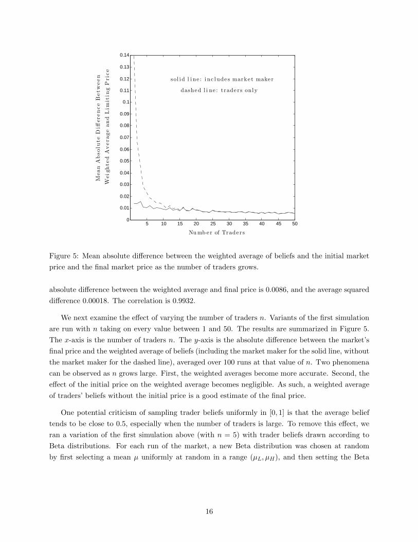
Figure 5: Mean absolute difference between the weighted average of beliefs and the initial market
price and the final market price as the number of traders grows.
absolute difference between the weighted average and final price is 0.0086, and the average squared
difference 0.00018. The correlation is 0.9932.
We next examine the effect of varying the number of traders n. Variants of the first simulation
are run with n taking on every value between 1 and 50. The results are summarized in Figure 5.
The x-axis is the number of traders n. The y-axis is the absolute difference between the market’s
final price and the weighted average of beliefs (including the market maker for the solid line, without
the market maker for the dashed line), averaged over 100 runs at that value of n. Two phenomena
can be observed as n grows large. First, the weighted averages become more accurate. Second, the
effect of the initial price on the weighted average becomes negligible. As such, a weighted average
of traders’ beliefs without the initial price is a good estimate of the final price.
One potential criticism of sampling trader beliefs uniformly in [0, 1] is that the average belief
tends to be close to 0.5, especially when the number of traders is large. To remove this effect, we
ran a variation of the first simulation above (with n = 5) with trader beliefs drawn according to
Beta distributions. For each run of the market, a new Beta distribution was chosen at random
by first selecting a mean µ uniformly at random in a range (µL, µH), and then setting the Beta
16
0 10
1
Weighted Ave rage of Be l i e f s ( I nc l uding Marke t Make r P ri or)
Lim
itin
gPrice
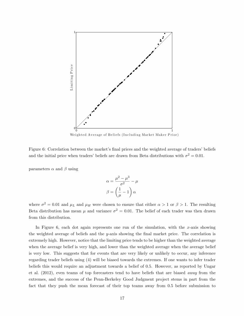
Figure 6: Correlation between the market’s final prices and the weighted average of traders’ beliefs
and the initial price when traders’ beliefs are drawn from Beta distributions with σ2 = 0.01.
parameters α and β using
α =µ2 − µ3
σ2− µ
β =
(1
µ− 1
)α
where σ2 = 0.01 and µL and µH were chosen to ensure that either α > 1 or β > 1. The resulting
Beta distribution has mean µ and variance σ2 = 0.01. The belief of each trader was then drawn
from this distribution.
In Figure 6, each dot again represents one run of the simulation, with the x-axis showing
the weighted average of beliefs and the y-axis showing the final market price. The correlation is
extremely high. However, notice that the limiting price tends to be higher than the weighted average
when the average belief is very high, and lower than the weighted average when the average belief
is very low. This suggests that for events that are very likely or unlikely to occur, any inference
regarding trader beliefs using (4) will be biased towards the extremes. If one wants to infer trader
beliefs this would require an adjustment towards a belief of 0.5. However, as reported by Ungar
et al. (2012), even teams of top forecasters tend to have beliefs that are biased away from the
extremes, and the success of the Penn-Berkeley Good Judgment project stems in part from the
fact that they push the mean forecast of their top teams away from 0.5 before submission to
17

0 1 2 3 4 5 6 7 8 9 100
0.01
0.02
0.03
0.04
0.05
0.06
0.07
0.08
CRRA Paramete r Rho
Mean
Absolu
teDifferenceBetween
Weighted
Averageand
Lim
itin
gPrice s ol i d l i ne : i nc l ude s marke t make r
dashed l i ne : trade rs onl y
Figure 7: Mean absolute difference between the weighted average of trader beliefs and the initial
market price and the final market price as the CRRA utility parameter ρ is varied.
IARPA. Figure 6 reveals that algorithmic prediction markets produce this effect automatically, and
this might explain why prediction markets outperform the unadjusted mean forecasts of their top
teams.
This effect arises because the bounded loss requirement causes prices to be adjusted very sharply
upwards if traders as a group accumulate a large long position, and very sharply downwards if they
are heavily short. The result is an inversion of the usual favorite-longshot bias found in peer-to-peer
markets and sports betting (Wolfers and Zitzewitz, 2006).
7.2 Varying Risk Aversion
We also examined the effect of varying the CRRA utility parameter ρ which controls the extent to
which the traders are risk averse. We repeated the first simulation above with ρ taking on every
multiple of 0.2 between 0 and 10. In the extreme case when ρ = 0, traders are risk neutral and
therefore our theory does not apply. In all other cases, traders are risk averse to different degrees.
The results are shown in Figure 7. While the approximation is reasonable throughout this
range, it is especially close when preferences are close to the log utility case. Values of ρ in the
range (1, 2) yield excellent approximations, reflecting levels of risk aversion slightly higher than in
18

the log utility case.
Since the market designer chooses the cost function, Equation (4) can be used to infer the
weighted average of trader beliefs from the limiting price. Our results show that this inference will
be most precise if the coefficient of relative risk aversion ρ lies in a particular range. But even if
this is not the case, (4) still provides a method for adjusting the limiting price in order to obtain
a better estimate of trader beliefs by taking into account the properties of the cost function. This
is superior in all cases to a naive interpretation of the market price that neglects the properties of
the algorithm being used to elicit beliefs.
8 Conclusions
Prediction markets based on automated market makers have become a fixture of the forecasting
landscape in a broad range of organizations, although little is understood about how market prices
should be interpreted in terms of trader beliefs and the attributes of cost functions. In this paper
we have taken a step towards filling this gap, by exploring the properties of limiting prices and
portfolios when risk averse traders interact repeatedly in arbitrary order with the market. Although
exact interpretations of the price in terms of trader beliefs is not possible in this environment, good
approximations can be obtained if traders are risk-averse and their beliefs are not distributed in a
manner that is too extreme.
There are at least two natural extensions of this work. First, one could allow for the possibility
that traders may deviate from myopic optimization if they believe that a more favorable price
will be available when they next have an opportunity to trade. This would require traders to
hold beliefs about the beliefs and trading strategies of others, as well as beliefs about the order of
trading. Given the complexity of the problem, it is likely that traders will use heuristics rather than
full-scale optimization in any departure from myopic behavior. It seems worth exploring variations
of our model with the incorporation of plausible heuristics.
Second, one could allow for both heterogeneous priors and differences in information. Clearly
the priors themselves cannot be common knowledge, since discovery of these is part of the rationale
for constructing the market. Hence traders would need to update not only beliefs about the state,
but also their beliefs about the beliefs of others as the process unfolds. In a model of sequential
and truthful belief announcements, Sethi and Yildiz (2012) show that information need not be fully
aggregated when priors are independently distributed and unobservable. Whether or not this is
also the case when information is revealed by trades rather than by belief announcements remains
an open question worthy of attention.
19
Appendix
Proof of Lemma 1. To prove the first case, assume that pi ≤ πt−1 and zi,t−1 ≥ 0. By the convexity
of C, showing that πt ≤ πt−1 is equivalent to showing that trader i does not select rt > 0. For this,
it suffices to show that he prefers rt = 0 to any rt > 0.
Consider some r > 0. By the convexity of C, the cost of purchasing r at time t is at least
πt−1r which is at least pir by our assumption that pi ≤ πt−1. The expected utility of trader i after
making this purchase is therefore upper bounded by the function
v(r) = piu(yi,t−1 + zi,t−1 − pir + r) + (1− pi)u(yi,t−1 − pir).
Taking the derivative of this function with respect to r yields
v′(r) = pi(1− pi)(u′(yi,t−1 + zi,t−1 − pir + r)− u′(yi,t−1 − pir)
).
Since u is concave (and so u′ is decreasing) and zi,t−1 ≥ 0, v′(r) is decreasing for r > 0. Since v(0)
is exactly the expected utility of trader i with r = 0 and v(r) is an upper bound on his utility when
r > 0, this implies that trader i prefers rt = 0 to any value rt > 0, as desired.
The proof of the second case is analogous to the proof of the first.
Proof of Lemma 2. To prove the first case, assume that pi ≥ πt−1 and zi,t−1 ≥ 0. We must show
that trader i does not select a bundle that would result in a price of πt > pi. For this, it suffices to
show that he would prefer to move the price to exactly pi rather than to any higher price.
Since any cost function based market is path independent, moving the price from πt−1 to πt
costs the same as moving the price from πt−1 to pi and then from pi to πt. Therefore, it suffices to
show that if trader i first moves the price to pi, he prefers to keep it there rather than subsequently
moving it to a higher value.
By the convexity of C, the price can be increased from πt−1 to pi only by purchasing a non-
negative number of shares. Let z ≥ zi,t−1 ≥ 0 be the asset position of trader i after this move.
Since his asset position is still non-negative, and the market price is now exactly equal to his beliefs,
we can apply Lemma 1 to immediately show that he prefers to keep the price at pi or decrease it
rather than increase it, which completes the proof.
The proof of the second case is analogous to the proof of the first, relying on the second case in
Lemma 1.
Proof of Proposition 1. Since π0 = p0 and p0 ∈ I by definition, it is clear that π0 ∈ I. Suppose, by
way of contradiction, that there exists t ≥ 1 such that πs ∈ I for all s < t and πt /∈ I. We consider
the case πt > pmax (the case πt < pmin may be proved analogously).
20

Let i = k(t), and suppose first that zi,t−1 = 0. If pi ≤ πt−1 then πt ≤ πt−1 ≤ pmax from Lemma
1 and the fact that πt−1 ∈ I, a contradiction. And if pi ≥ πt−1 then πt ≤ pi ≤ pmax from Lemma 2
and the fact that pi ∈ I, a contradiction.
Now suppose that zi,t 6= 0. Then there exists s < t such that k(s) = i and k(t′) 6= i for all
t′ ∈ {s+ 1, ..., t− 1}. We know that (yi,t−1, zi,t−1) is an optimal portfolio for i at market state qs,
when the market price is πs ≤ pmax. If πt−1 = πs then i will not change his portfolio in period t,
so πt = πt−1 ≤ pmax, a contradiction. If πt−1 > πs then i will sell in period t, so πt < πt−1 ≤ pmax,
a contradiction.
Finally, if πt−1 < πs, then i will buy in period t. Any such transaction may be viewed as taking
two steps in sequence: buy until the price reaches πs, and then buy or sell to reach the new optimum.
After the first stage the market state will be qs and the endowment will be (y, z) where y < yi,t−1
and z > zi,t−1. Since i did not want to buy or sell at this market state with portfolio (yi,t−1, zi,t−1),
he will want to sell with portfolio (y, z). Hence πt < πt−1 ≤ pmax, a contradiction.
Proof of Lemma 3. Suppose that trader i with endowment (y, z) is considering purchasing r units
of the asset at some market state q, and let cq(r) = C(q + r) − C(q) denote the cost of this
transaction. If r < 0, this is a sale and the cost is negative. The expected utility of trader i after
this transaction is given by
piu(y − cq(r) + z + r) + (1− pi)u(y − cq(r)).
Taking the derivative with respect to r gives
pi(1− c′q(r))u′(y − cq(r) + z + r)− (1− pi)c′q(r)u′(y − cq(r)). (5)
Consider any t such that s(t) > 0 and let i = k(t). For notational simplicity, we will write s in
place of s(t). We know that trader i would not want to buy or sell at endowment (yi,s, zi,s) and
market state q such that C ′(q) = c′q(0) = πs; otherwise, the path independence of the cost function
implies that trader i would not have left the price in this state at time s. From Equation 5, this
tells us that
pi(1− πs)u′(yi,s + zi,s)− (1− pi)πsu′(yi,s) = 0 (6)
Now consider the decision of trader i at time t. Since the endowment of trader i at the start of
period t is precisely (yi,s, zi,s) and the current price is πt−1, Equation 5 tells us that trader i would
want to buy a positive quantity of the asset if and only if
pi(1− πt−1)u′(yi,s + zi,s)− (1− pi)πt−1u′(yi,s) > 0.
From Equation 6, this holds if and only if πt−1 < πs. Similarly, trader i would want to sell a
positive quantity (or buy a negative quantity) if and only if πt−1 > πs.
21
First consider the case in which πt−1 < πs, so the trader wants to buy. Suppose that i submits
an order that restores the market to the state q such that C ′(q) = cq(0) = πs. Let (y′, z′) denote
the resulting endowment, and note that y′ < yi,s and y′ + z′ > yi,s + zi,s. We shall show that at
this endowment and price, the trader now wishes to sell. To see this, consider a purchase (possibly
negative) of r units starting from the endowment (y′, z′) at market state q. As before, the expected
utility is given by
piu(y′ − cq(r) + z′ + r) + (1− pi)u(y′ − cq(r)),
and its derivative at r = 0 is
pi(1− πs)u′(y′ + z′)− (1− pi)πsu′(y′).
This must be less than 0 by Equation 6, the concavity of u, and the fact that y′ < y and y′+z′ > y+z.
By path independence of the cost function, this implies that while i would like to buy at price πt−1,
he would not buy enough to push the price back to πs, yielding the result.
The proof for the case in which πt−1 > πs is analogous.
Proof of Lemma 4. Define
Γ = {(y, z) | y > 0, y + z > 0},
and define the function ψ : Γ→ (0, 1) as
ψ(y, z) =piu′(y + z)
piu′(y + z) + (1− pi)u′(y).
From (6), the endowment (y, z) ∈ Γ is optimal for trader i at price ψ(y, z) in the sense that a trader
with portfolio (y, z) would not want to buy or sell if the current price were ψ(y, z). Note that ψ is
continuous since u is smooth, so the inverse image ψ−1(E) of any closed set E ⊂ (0, 1) is closed.
In particular, ψ−1({π}) is closed for any π ∈ I = [pmin, pmax].
Consider any t such that s(t) > 0, and let s = s(t) and i = k(t). Since πs ∈ I and limw→0 u′(w) =
∞, optimal portfolios will satisfy the non-negative wealth constraints with strict inequality in all
periods. That is, (yi,s, zi,s) ∈ Γ. By Lemma 3, the choice problem faced by trader i in period t
with budget y = yi,s and assets z = zi,s may be expressed as follows: choose α ∈ [0, 1) to maximize
piu(y − cπs,πt−1(α) + z + rπs,πt−1(α)) + (1− pi)u(y − cπs,πt−1(α)),
where rπs,πt−1(α) is the (positive or negative) quantity of assets that trader i would need to purchase
to bring the market price to πt = απs + (1 − α)πt−1, and cπs,πt−1(α) is the cost of this purchase.
The bounded loss of C implies that these quantities must exist since it must be possible to move
the market price to anything in (0, 1) (Abernethy et al., 2011, 2013). Furthermore, one can easily
verify that for any given values of πs and πt−1, rπs,πt−1(α) and cπs,πt−1(α) are both continuous since
22
the cost function C is smooth and convex. The necessary and sufficient condition for a maximum
is
pi(r′πs,πt−1
(α)− c′πs,πt−1(α))u′(y − cπs,πt−1(α) + z + rπs,πt−1(α))
−(1− pi)c′πs,πt−1(α)u′(y − cπs,πt−1(α)) = 0.
For any given tuple (y, z, πs, πt−1) with πs 6= πt−1, this condition implies a unique solution
α(y, z, πs, πt−1) by Lemma 3. By the continuity of u(·), rπs,πt−1(·), and cπs,πt−1(·), α(·) is also
continuous where it is defined.
Note that for any η > 0, α(·) is well-defined on the domain
∆ ={
(y, z, πs, πt−1) ∈ R4 | (πs, πt−1) ∈ [pmin, pmax]2, (y, z) ∈ ψ−1({πs}), |πs − πt−1| ≥ η}.
Since ψ−1({πs}) is closed and bounded, ∆ is compact. Since compactness is preserved by continuous
functions, α must also have a compact range, which excludes α = 1 by Lemma 3; although some
states in ∆ may not be reachable in the market, the proof of Lemma 3 holds for all states in this
set. Hence the range of α over domain ∆ must have a maximum element α(η) < 1.
Proof of Lemma 6. Note that for any η > 0, there exist ε > 0 and δ > 0 such that
η > ε+δ + α(η)ε
1− α(η), (7)
since α(η) < 1 from Lemma 4. Let η > 0 be given and consider any positive ε and δ consistent
with (7). By definition of π, there exists t′ such that, for all t > t′ − n, πt < π + ε. Consider any
τ > t′ such that πτ > π − δ. Clearly πτ−n < π + ε. By Lemma 3 we have
πτ = ατπτ−n + (1− ατ )πτ−1. (8)
This implies
(1− ατ )πτ−1 = πτ − ατπτ−n > π − δ − ατ (π + ε).
Hence
πτ−1 > π − δ + ατε
1− ατ> πτ −
(ε+
δ + ατε
1− ατ
)(9)
where the last inequality follows from the fact that πτ < π + ε.
We claim that
πτ−1 > πτ − η.
Suppose not. Then πτ − πτ−1 ≥ η, which by (8) implies that πτ−n − πτ−1 ≥ η, and ατ ≤ α(η).
Hence from (9), we obtain
πτ−1 > πτ −(ε+
δ + α(η)ε
1− α(η)
),
23

which implies πτ−1 > πτ − η from (7), a contradiction. Hence πτ−1 > πτ − η. Note that δ < η from
(7), so
πτ−1 > π − δ − η > π − 2η.
Setting η = γ/2 yields the desired result.
Proof of Theorem 1. From Lemma 6, for any γ > 0, there exists t′ ∈ N and a sequence of positive
numbers δ1, ..., δn such that
γ = δ1 > δ2 > ... > δn > 0
and, for all t > t′ and i = 2, ..., n,
πt+i > π − δi =⇒ πt+i−1 > π − δi−1.
Furthermore, there exists t > t′ such that πt+n ≥ π > π−δn. Suppose that π > π and set γ = π−π.
Then there exists a sequence of n consecutive prices πt+1, ..., πt+n all of which exceed π. Hence
πt+n > π, a contradiction.
Proof of Proposition 2. Consider a trader with belief p, portfolio (y, z), facing price π. From the
first order condition for optimality, this trader will choose to remain at this portfolio if and only if
p(1− π)u′(y + z) = π(1− p)u′(y),
or
π =pu′(y + z)
pu′(y + z) + (1− p)u′(y).
Concavity of u implies that
π =pu′(y + z)
pu′(y + z) + (1− p)u′(y)< p
if and only if z > 0. Similarly, π > p if and only if z < 0. Since the terminal portfolio is optimal
given the terminal price, the result follows.
24
References
Jacob Abernethy, Yiling Chen, and Jennifer Wortman Vaughan. An optimization-based framework for
automated market-making. In Proceedings of the 12th ACM Conference on Electronic Commerce (ACM
EC), 2011.
Jacob Abernethy, Yiling Chen, and Jennifer Wortman Vaughan. Efficient market making via convex opti-
mization, and a connection to online learning. ACM Transactions on Economics and Computation, 1(2):
12:1–12:39, 2013.
Robert J. Aumann. Agreeing to disagree. Annals of Statistics, 4(6):1236–1239, 1976.
Joyce Berg, Robert Forsythe, Forrest Nelson, and Thomas Rietz. Results from a dozen years of election
futures markets research. In Handbook of Experimental Economics Results, Volume 1, 2008.
Philip Delves Broughton. Prediction markets: value among the crowd. Financial Times, April 2013.
Robert Charette. An internal futures market. Information Management, March 2007.
Kay-Yut Chen and Charles Plott. Information aggregation mechanisms: Concept, design and field imple-
mentation. Social Science Working Paper no. 1131. Pasadena: California Institute of Technology, 2002.
Yiling Chen and David M. Pennock. A utility framework for bounded-loss market makers. In Proceedings
of the 23rd Conference on Uncertainty in Artificial Intelligence (UAI), 2007.
Yiling Chen, Mike Ruberry, and Jennifer Wortman Vaughan. Designing informative securities. In Proceedings
of the 28th Conference on Uncertainty in Artificial Intelligence (UAI), 2012.
Yiling Chen, Mike Ruberry, and Jennifer Wortman Vaughan. Cost function market makers for measurable
spaces. In Proceedings of the 14th ACM Conference on Electronic Commerce (ACM EC), 2013.
Bo Cowgill, Justin Wolfers, and Eric Zitzewitz. Using prediction markets to track information flows: Evidence
from Google. Working Paper, 2009.
Duncan K. Foley. A statistical equilibrium theory of markets. Journal of Economic Theory, 62(2):321–345,
1994.
John D. Geanakopolos and Heraklis M. Polemarchakis. We can’t disagree forever. Journal of Economic
Theory, 28(1):192–200, 1982.
Steven Gjerstad. Risk aversion, beliefs, and prediction market equilibrium. Working Paper, Economic Science
Laboratory, University of Arizona, 2004.
Frank H. Hahn and Takashi Negishi. A theorem on non-tatonnement stability. Econometrica, 30(3):463–469,
1962.
Robin D. Hanson. Combinatorial information market design. Information Systems Frontiers, 5(1):107–119,
2003.
Robin D. Hanson. Logarithmic market scoring rules for modular combinatorial information aggregation.
Journal of Prediction Markets, 1(1):1–15, 2007.
25

Friedrich A. Hayek. The use of knowledge in society. American Economic Review, 35(4):519–530, 1945.
Krishnamurthy Iyer, Ramesh Johari, and Ciamic C. Moallemi. Information aggregation and allocative
efficiency in smooth markets. Working Paper, 2010.
Charles F. Manski. Interpreting the predictions of prediction markets. Economics Letters, 91(3):425–429,
2006.
Michael Ostrovsky. Information aggregation in dynamic markets with strategic traders. Econometrica, 80
(6):2595–2648, November 2012.
Abraham Othman and Tuomas Sandholm. When do markets with simple agents fail? In Proceedings of the
9th International Conference on Autonomous Agents and Multiagent Systems (AAMAS), 2010.
David M. Pennock. Aggregating Probabilistic Beliefs: Market Mechanisms and Graphical Representations.
PhD thesis, The University of Michigan, 1999.
Rajiv Sethi and Muhamet Yildiz. Public disagreement. American Economic Journal: Microeconomics, 4(3):
57–95, 2012.
Lyle Ungar, Barb Mellors, Ville Satopaa, Jon Baron, Phil Tetlock, Jaime Ramos, and Sam Swift. The good
judgment project: A large scale test of different methods of combining expert predictions. AAAI Technical
Report FS-12-06, 2012.
Justin Wolfers and Eric Zitzewitz. Interpreting prediction market prices as probabilities. NBER Working
Paper No. 12200, 2006.
26
Related Documents


