Behavioural Finance, Options Markets and Financial Crises

Durham E-Theses

Behavioural Finance, Options Markets and Financial

Crises: Application to the UK Market 1998-2010

WHITFIELD, IAN,ALAN

How to cite:

WHITFIELD, IAN,ALAN (2013) Behavioural Finance, Options Markets and Financial Crises: Application

to the UK Market 1998-2010, Durham theses, Durham University. Available at Durham E-Theses Online:http://etheses.dur.ac.uk/7714/

Use policy

The full-text may be used and/or reproduced, and given to third parties in any format or medium, without prior permission orcharge, for personal research or study, educational, or not-for-pro�t purposes provided that:

• a full bibliographic reference is made to the original source

• a link is made to the metadata record in Durham E-Theses

• the full-text is not changed in any way

The full-text must not be sold in any format or medium without the formal permission of the copyright holders.

Please consult the full Durham E-Theses policy for further details.

http://www.dur.ac.uk

http://etheses.dur.ac.uk/7714/

http://etheses.dur.ac.uk/7714/

http://etheses.dur.ac.uk/policies/

Academic Support O�ce, Durham University, University O�ce, Old Elvet, Durham DH1 3HPe-mail: [email protected] Tel: +44 0191 334 6107

http://etheses.dur.ac.uk

2

http://etheses.dur.ac.uk

Behavioural Finance, Options Markets

and Financial Crises: Application to the

UK Market 1998-2010

By Ian Alan Whitfield

Submitted for the degree of

Doctor of Philosophy

Durham Business School

University of Durham

1st February 2013

javascript:ClickThumbnail(82)

i

Behavioural Finance, Options Markets and Financial Crises: Application to the

UK Market 1998-2010

By Ian Alan Whitfield

Abstract

This thesis examines the relationship between behavioural finance and options

markets. Particular focus is on the analysis of option prices, implied volatility and

trading activity which in turn provides insights into predictability, momentum and

overreaction.

The thesis is contextualised by a general to specific evaluation of the literature that

forms the basis of the behavioural finance paradigm. The review is extended to

analyse the extent to which support for the behavioural finance approach has been

produced by research on options. Behavioural finance retains an element of

controversy as it runs counter to a key pillar of neoclassical finance, the efficient

markets hypothesis. Hence the onus is on researchers in this field to produce

evidence that refutes the notion of market efficiency and to build models with

testable implications that are better able to capture the mechanics of financial

markets.

This thesis is motivated by a desire to investigate, in detail, key aspects of human

behaviour and to test whether they are particularly apparent in options markets. It is

important to study the information which can be extracted from options data and to

analyse whether this has any predictive power for spot prices. By extension, it is of

further interest to examine whether movements in spot prices exert influence on

option prices. In particular, aspects of options that capture human behaviour such as

pricing of puts relative to calls, implied volatility, trading volume and open interest.

The topical relevance of the work is highlighted by thorough application to the UK

ii

market during two recent periods of intense financial turbulence; the bursting of the

dotcom bubble in 2001 and the liquidity/banking crisis of 2007/8.

The empirical work examines the pricing of exchange-traded options relative to

theoretical values, the forecasting performance of implied volatility indexes, the

ability of trading volume and open interest to capture behavioural aspects of trading

behaviour, and momentum and overreaction effects. Hence the work provides a

unique and thorough investigation into behavioural finance and options markets in

the UK. Results indicate an important role for investor sentiment although they do

not necessarily indicate exploitable inefficiencies.

iii

Declaration

No part of this thesis has been submitted elsewhere for any other

degree or qualification in this or any other university. It is all my own

work unless referenced to the contrary in the text.

Copyright © 2013 by Ian Alan Whitfield

The copyright of this thesis rests with the author. No quotations from it

should be published without the author‟s prior written consent and

information derived from it should be acknowledged.

iv

Acknowledgements

I would like to thank my colleagues for their advice, support and

patience during the preparation of this thesis. I am indebted to

Toby Watson for invaluable assistance through numerous data

collection and organisation crises. Also sincere thanks to David

Barr, Arthur Walker and Ian Lincoln for useful and insightful

guidance and comments. All of your help is much appreciated.

v

Table of Contents

ABSTRACT i

DECLARATION iii

ACKNOWLEDGEMENTS ix

LIST OF FIGURES x

LIST OF TABLES xI

INTRODUCTION 1

CHAPTER 1

Behavioural Finance; Past, Present and Future 9

1.1 Introduction 10

1.2 The Efficient Markets Hypothesis 12

1.2.1 Theoretical basis of the efficient markets hypothesis 13

1.2.2 Empirical support for the efficient markets hypothesis 15

1.3 Behavioural finance building block one: psychology 18

1.3.1 Beliefs 19

1.3.1.1 Framing 19

1.3.1.2 Overconfidence 20

1.3.1.3 Optimism and wishful thinking 27

1.3.1.4 Representativeness 29

1.3.1.5 Conservatism 30

1.3.1.6 Confirmation bias 30

1.3.1.7 Anchoring 30

1.3.1.8 Cognitive dissonance 31

1.3.1.9 Memory bias 31

1.3.2 Preferences: from expected utility to prospect theory 32

1.4 Behavioural finance building block two: limits to arbitrage 43

1.5 The noise trader challenge to EMH 49

vi

1.6 Empirical challenges to EMH 51

1.6.1 Excess volatility 51

1.6.2 Anomalies in returns 57

1.7 Overreaction and underreaction 59

1.7.1 Overreaction 61

1.7.2 Underreaction 70

1.7.3 Reconciling overreaction and underreaction 73

1.8 The closed end fund puzzle 76

1.9 The equity premium puzzle 87

1.10 Collective behaviour 90

1.11 Behavioural Corporate Finance 94

1.12 Speculative bubbles 96

1.13 Investor behaviour and moods 99

1.14 Future directions of behavioural finance 102

1.14.1 Stock markets 102

1.14.2 Derivative markets 103

1.14.3 Key criticisms of behavioural finance 103

1.14.4 The next paradigm? 103

1.15 Conclusion 105

CHAPTER 2

Behavioural Finance and Options Markets 106

2.1 Introduction 107

2.2 Violations of rational pricing bounds 107

2.3 Violations of put-call parity 110

2.4 Deviations of market prices from theoretical prices 113

2.5 Overreaction and underreaction in options markets 114

2.6 Momentum Effects and the Demand Parameter in Option Pricing 121

2.7 Irrational early exercise of American-style call options 129

vii

2.8 Trading behaviour of options market participants 132

2.9 Conclusion 135

CHAPTER 3

Premiums on Stock Index Options and Expectations of the Early 21st Century

Bear Market:

Evidence from FTSE100 European Style Index Options 136

3.1 Introduction, motivation and literature 137

3.2 Hypothesis and methodology 146

3.2.1 Call/put premiums 147

3.2.2 Black-Scholes prices 148

3.2.2.1 The model 148

3.2.2.2 Risk-neutral valuation 154

3.2.2.3 The model applied to FTSE100 index options 155

3.2.3 Implied volatility 158

3.3 Data 163

3.4 Results and analysis 169

3.4.1 Call/put premiums 169

3.4.2 Black-Scholes prices 176

3.4.3 Implied volatilities 185

3.5 Volatility Smiles and the Risk Neutral Distribution 190

3.6 Conclusion 195

CHAPTER 4

Was the 2007 Crisis Expected?

An Analysis of Implied Volatility in UK Index Options Markets 197

4.1 Introduction and motivation 198

4.2 Literature 200

viii

4.3 Initial tests to examine the VIX/VFTSE relationship 209

4.3.1 Introduction 209

4.3.2 Data 209

4.3.3 OLS regression analysis and unit root tests 211

4.3.4 Granger causality tests 213

4.3.5 Cointegration tests ` 215

4.3.6 Conclusion 216

4.4 The VIX and the UK equity market in the pre-financial crisis, crisis and

post-crisis periods 217


4.4.2 Data 217

4.4.3 Methodology 219

4.4.4 Results 226


4.5 The VUK and the UK equity market before and during the financial crisis

237


4.5.2 Data 210


4.5.4 Results 243


CHAPTER 5

An Analysis of Trading Volume and Open Interest in UK FTSE100 Index and Individual Equity Options Markets during the 2007-2008 Financial Crisis

254

5.1 Introduction and motivation 255

5.2 Literature 258

5.3 Data 263

ix

5.4 Methodology 272

5.5 Results 276

5.6 A behavioural perspective on trading volume and open interest 295

5.7 Conclusion 301

CHAPTER 6

On the Presence of Momentum Effects and Short-Term Overreaction in

the UK Index Options Market 2006-2010 303

6.1 Introduction 304

6.2 Data 306

6.3 Momentum 307


6.3.2 Results 310

6.3.2.1 Put-Call Parity Boundary Violation Tests 310

6.3.3 Implied Volatility Spread Results 315

6.3.3.1 Sub-Periods 318

6.4 Short-Run Overreaction 320


6.5 Discussion and Conclusion 333

CHAPTER 7 335

Summary, Conclusions and Suggestions for Future Research 260

7.1 Summary of issues and key contributions 336

7.2 Future research 341

BIBLIOGRAPHY 342

Appendix 1

Cox, Ross and Rubinstein (1979) binomial asset pricing model 362

Appendix 2

The Heston (1993) model as applied to the tests of Poteshman (2001) 367

x

Appendix 3 Constituents of equity portfolio of financial stocks with associated LIFFE

exchange-traded equity options 369

xi

List of Figures

1.1 Building Blocks of Behavioural Finance 10

1.2 Loss Aversion 37

3.1 FTSE100 Stock Index 1/6/1998-12/9/2003 165

3.2 FTSE100 Stock Index 1/9/2000-22/3/2001 173

3.4 Implied Volatility Skews 190

3.5 FTSE100 Stock Index 1/8/1997-1/8/1999 173

4.1 Time Series Graph of the VIX 2007-2009 208

4.2 Time Series Graph of the VIX and VFTSE 2010-2011 (Closing) 210

4.3 GARCH News Impact Curves 221

4.4 FTSE100 Daily Returns and the VUK: 2006-2010 241

4.5 Daily Returns and the VUK: June 2007 through December 2008 242

4.6 FTSE100 Stock Index May 2007 – December 2008 250

xii

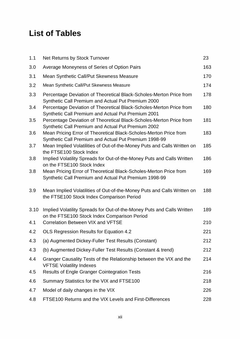
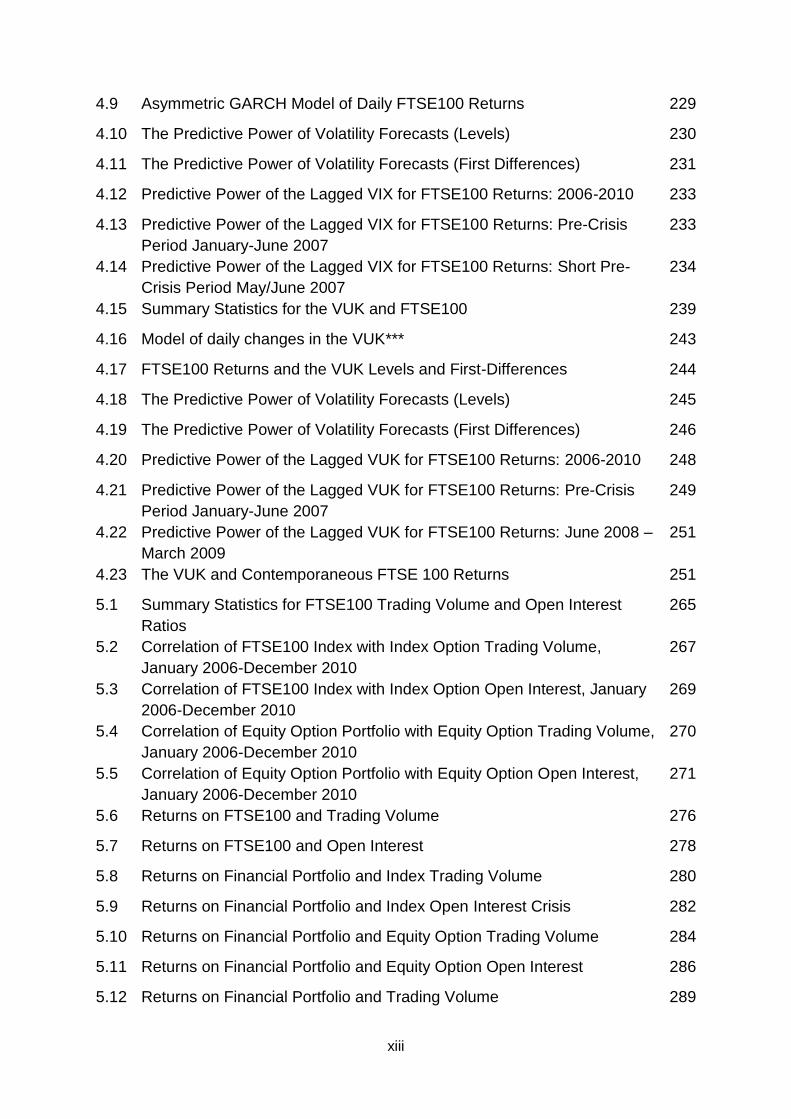
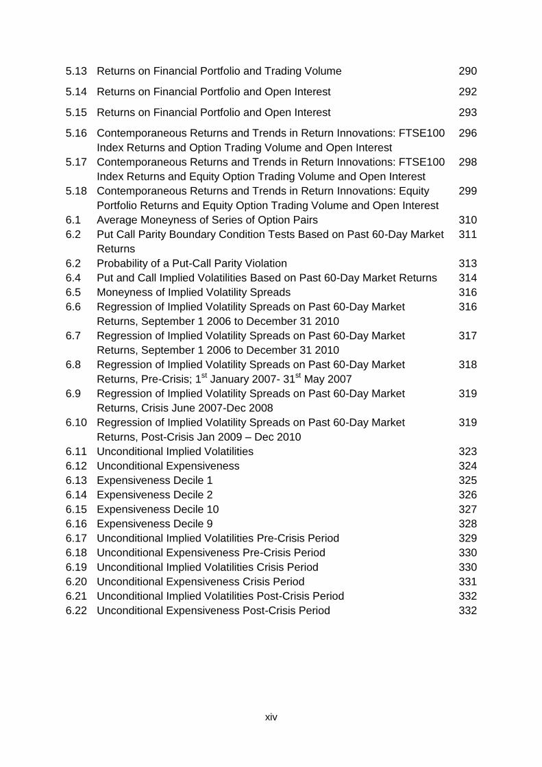
List of Tables

1.1 Net Returns by Stock Turnover 23

3.0 Average Moneyness of Series of Option Pairs 163

3.1 Mean Synthetic Call/Put Skewness Measure 170

3.2 Mean Synthetic Call/Put Skewness Measure 174

3.3 Percentage Deviation of Theoretical Black-Scholes-Merton Price from

Synthetic Call Premium and Actual Put Premium 2000

178



180



181

3.6 Mean Pricing Error of Theoretical Black-Scholes-Merton Price from

Synthetic Call Premium and Actual Put Premium 1998-99

183

3.7 Mean Implied Volatilities of Out-of-the-Money Puts and Calls Written on

the FTSE100 Stock Index

185

3.8 Implied Volatility Spreads for Out-of-the-Money Puts and Calls Written

on the FTSE100 Stock Index

186

3.8 Mean Pricing Error of Theoretical Black-Scholes-Merton Price from

Synthetic Call Premium and Actual Put Premium 1998-99

169

3.9 Mean Implied Volatilities of Out-of-the-Money Puts and Calls Written on

the FTSE100 Stock Index Comparison Period

188

3.10 Implied Volatility Spreads for Out-of-the-Money Puts and Calls Written

on the FTSE100 Stock Index Comparison Period

189

4.1 Correlation Between VIX and VFTSE 210

4.2 OLS Regression Results for Equation 4.2 221

4.3 (a) Augmented Dickey-Fuller Test Results (Constant) 212

4.3 (b) Augmented Dickey-Fuller Test Results (Constant & trend) 212

4.4 Granger Causality Tests of the Relationship between the VIX and the

VFTSE Volatility Indexes

214

4.5 Results of Engle Granger Cointegration Tests 216

4.6 Summary Statistics for the VIX and FTSE100 218

4.7 Model of daily changes in the VIX 226

4.8 FTSE100 Returns and the VIX Levels and First-Differences 228

xiii

4.9 Asymmetric GARCH Model of Daily FTSE100 Returns 229

4.10 The Predictive Power of Volatility Forecasts (Levels) 230

4.11 The Predictive Power of Volatility Forecasts (First Differences) 231

4.12 Predictive Power of the Lagged VIX for FTSE100 Returns: 2006-2010 233

4.13 Predictive Power of the Lagged VIX for FTSE100 Returns: Pre-Crisis

Period January-June 2007

233

4.14 Predictive Power of the Lagged VIX for FTSE100 Returns: Short Pre-

Crisis Period May/June 2007

234

4.15 Summary Statistics for the VUK and FTSE100 239

4.16 Model of daily changes in the VUK*** 243

4.17 FTSE100 Returns and the VUK Levels and First-Differences 244

4.18 The Predictive Power of Volatility Forecasts (Levels) 245

4.19 The Predictive Power of Volatility Forecasts (First Differences) 246

4.20 Predictive Power of the Lagged VUK for FTSE100 Returns: 2006-2010 248

4.21 Predictive Power of the Lagged VUK for FTSE100 Returns: Pre-Crisis

Period January-June 2007

249

4.22 Predictive Power of the Lagged VUK for FTSE100 Returns: June 2008 –

March 2009

251

4.23 The VUK and Contemporaneous FTSE 100 Returns 251

5.1 Summary Statistics for FTSE100 Trading Volume and Open Interest

Ratios

265

5.2 Correlation of FTSE100 Index with Index Option Trading Volume,

January 2006-December 2010

267

5.3 Correlation of FTSE100 Index with Index Option Open Interest, January

2006-December 2010

269

5.4 Correlation of Equity Option Portfolio with Equity Option Trading Volume,


270

5.5 Correlation of Equity Option Portfolio with Equity Option Open Interest,


271

5.6 Returns on FTSE100 and Trading Volume 276

5.7 Returns on FTSE100 and Open Interest 278

5.8 Returns on Financial Portfolio and Index Trading Volume 280

5.9 Returns on Financial Portfolio and Index Open Interest Crisis 282

5.10 Returns on Financial Portfolio and Equity Option Trading Volume 284

5.11 Returns on Financial Portfolio and Equity Option Open Interest 286

5.12 Returns on Financial Portfolio and Trading Volume 289

xiv

5.13 Returns on Financial Portfolio and Trading Volume 290

5.14 Returns on Financial Portfolio and Open Interest 292

5.15 Returns on Financial Portfolio and Open Interest 293

5.16 Contemporaneous Returns and Trends in Return Innovations: FTSE100

Index Returns and Option Trading Volume and Open Interest

296

5.17 Contemporaneous Returns and Trends in Return Innovations: FTSE100

Index Returns and Equity Option Trading Volume and Open Interest

298

5.18 Contemporaneous Returns and Trends in Return Innovations: Equity

Portfolio Returns and Equity Option Trading Volume and Open Interest

299

6.1 Average Moneyness of Series of Option Pairs 310

6.2 Put Call Parity Boundary Condition Tests Based on Past 60-Day Market

Returns

311

6.2 Probability of a Put-Call Parity Violation 313

6.4 Put and Call Implied Volatilities Based on Past 60-Day Market Returns 314

6.5 Moneyness of Implied Volatility Spreads 316

6.6 Regression of Implied Volatility Spreads on Past 60-Day Market

Returns, September 1 2006 to December 31 2010

316



317


Returns, Pre-Crisis; 1st January 2007- 31st May 2007

318


Returns, Crisis June 2007-Dec 2008

319


Returns, Post-Crisis Jan 2009 – Dec 2010

319

6.11 Unconditional Implied Volatilities 323

6.12 Unconditional Expensiveness 324

6.13 Expensiveness Decile 1 325




6.17 Unconditional Implied Volatilities Pre-Crisis Period 329

6.18 Unconditional Expensiveness Pre-Crisis Period 330

6.19 Unconditional Implied Volatilities Crisis Period 330

6.20 Unconditional Expensiveness Crisis Period 331

6.21 Unconditional Implied Volatilities Post-Crisis Period 332

6.22 Unconditional Expensiveness Post-Crisis Period 332

1

INTRODUCTION

The overall objective of this thesis is to examine options markets for evidence of

behavioural factors. Rather than evaluate behavioural factors in options more

generally, this study focuses on a fairly recent time period containing two sub-

periods of high market volatility; the burst of the dot com bubble in 2000 and the

financial crisis of 2007/8. A number of approaches are adopted to pursue the central

objective. The behaviour of option prices and implied volatility are examined prior to,

and during the burst of the dot com bubble in order to establish whether they contain

any predictive ability for future market moves. A UK implied volatility index is

constructed which covers the period before, during and after the 2007/8 crisis. The

index‟s forecasting ability for future volatility and predictive ability for future market

returns is then analysed. A sentiment measure is constructed, using trading volume

and open interest of FTSE100 index options and options written on the stocks of

financial stocks, and used to test for predictive power. Furthermore, the sentiment

measure is analysed following sharp, consecutive short-term market moves of a

consistent sign. The objective is to test whether trading behaviour is induced by

perceived trends. Standard option pricing models do not incorporate price pressure

as a parameter. This study hypothesises that demand is an important parameter in

the pricing of options. A non-parametric approach is adopted to test for momentum

effects before, during and after the 2007/8 financial crisis. The non-parametric

approach involves evaluating put-call parity violations following 60-day positive and

negative market returns. Momentum tests are also performed by employing a

parametric approach which involves analysis of the behaviour of implied volatility

spreads following positive and negative market returns. If momentum effects are

2

identified in options markets then this implies that demand provides an additional

parameter in option pricing. Finally the relationship between implied volatility and

realised volatility, conditional on short-run significant price changes in the underlying

index, is examined. The hypothesis to be tested is that options market investors in

the UK overreact to short term moves in the underlying index.

The thesis begins by contextualising the empirical chapters. This is done by

reviewing important historical and more recent literature in the field of behavioural

finance generally. This is followed by a second review chapter which focuses on

research into behavioural finance and options markets. Behavioural finance presents

an important and growing challenge to the neoclassical finance paradigm and

involves the application of cognitive psychology to analyse human behaviour in

financial markets. Why is behavioural finance important? The desire to build

alternative models has arisen because neoclassical finance theory does not appear

to explain adequately a number of aspects of human behaviour within financial

markets. For example, why do individuals trade frequently? What rules or guidelines

do investors use to construct portfolios and how well do these portfolios perform?

Why do we observe variation in returns across investments in financial assets for

reasons other than risk‟ or more precisely how investors perceive risk?1 Questions of

this nature do not appear to be satisfactorily addressed by models of traditional

finance and pose significant problems for the efficient markets hypothesis.

A substantial body of literature within finance, and particularly within asset-pricing, is

based on the assumption of an efficient capital market (see inter alia Kendall, 1953,

Fama, 1970) and rational investor behaviour. In an efficient capital market the prices

of securities will reflect all relevant available information. This implies that any new

1 Key questions adapted from Subrahmanyam (2007).

3

information revealed about a firm will be recognised by market participants who will

then update their views accordingly. Thus the information will be rapidly impounded

into that firm‟s security prices and investors will not be able to make consistent

abnormal profits by trading on the basis of information after it has been revealed. It

follows that investors should only be able to consistently make fair returns on

average, based upon the risks associated with the securities they have invested in.

In such circumstances fairly and correctly priced securities provide reliable

information on which to base financial decisions.

The relatively new research area of behavioural finance runs counter to the efficient

markets hypothesis and the notion of the fully rational investor. A key aspect of

behavioural finance theories is that investors make systematic errors, which can

result in a sustained shift of security prices away from their fundamental values.

Increasingly, behavioural finance is addressing, and in many cases providing

plausible explanations of, many apparent inefficiencies, anomalies and irrational

investor behaviour in financial markets. Some key research topics and examples of

interesting contributions to the literature are as follows:

Excess Volatility (Shiller, 1981, LeRoy and Porter, 1981)

Overreaction (DeBondt and Thaler, 1985, Daniel, Hirshleifer and Subramanyam, 1998)

Disposition effect (Shefrin and Statman, 1985)

Predictability (Fama and French, 1988)

Conservatism and underreaction (Barberis, Shleifer and Vishny, 1998)

Closed end fund puzzle (Lee, Shleifer and Thaler, 1991, Shleifer, 2000)

Excessive trading (Odean, 1999)

4

Abnormal price movements relating to events such as mergers, share

repurchases and IPOs (Ikenberry, Lakonishok and Vermaelen, 1995)

Collective behaviour (Sentana and Wadhwani, 1992)

Speculative bubbles in equity markets in the late 1990s and subsequent

downturn in 2000/2001. Irrational Exuberance (Shiller, 2000).

The behavioural arguments offered in much of the literature have gained momentum

over recent years and have become increasingly persuasive. In particular, these

arguments provide an attractive alternative approach when considered in the context

of the difficulties that traditional models face in explaining many previously

unexplained market phenomena.

It may at first seem counter-intuitive to analyse behavioural finance in derivative

markets and in particular options markets. In conventional finance the price of a

derivative is tied strongly to that of the underlying asset by arbitrage conditions. For

example, the Black-Scholes (1973) option pricing model is derived by constructing

an instantaneously riskless no-arbitrage portfolio of stocks and options. If the cash

flows of the derivative can be replicated by implementing a dynamic strategy using

stocks and riskless bonds then the derivative is regarded as a redundant asset.

However, the fact that options not only exist but are also extensively traded indicates

that market participants do not perceive them as redundant assets. The options

market provides investors with the opportunity to enhance their utility by expanding

the range of risk management and leverage opportunities available. An option gives

the holder the opportunity to transfer risk to another individual who, in return for a

fee, is willing to accept that risk. Hence investors are able to avoid regret by using

5

the options market. Options also facilitate leveraged speculation in stocks with

limited downside risk. Options, particularly index options have low transactions costs

compared to the underlying assets. For example, contrast the cost of shorting all of

the constituent stocks in the FTSE100 in their value-weighted proportions with the

cost of buying a FTSE100 put option. Furthermore, it is not necessarily correct to

assume that the options market is populated by the same individuals who populate

the equity market. Nor should it be assumed that each population share the same

degree of sophistication.

Relatively recent literature has been published which identifies behavioural issues

such as overreaction, momentum, predictability, loss aversion and narrow framing in

options markets or, more precisely, individuals trading in these markets. It is

therefore a worthwhile exercise to compile a significant quantity of theory and

evidence on this apparently anomalous activity into a single study and to perform

some further empirical analysis to potentially produce evidence of behavioural biases

in options markets. In particular it is important to investigate whether we can identify

aspects of investor behaviour before, during and after periods of significant market

turbulence from options market data. In this study the „dotcom bubble‟ and „liquidity

crisis‟ periods of the early 21st century will be examined by focusing on the key

indicators of option market activity identified above. Options can be used to reveal

the risk-neutral distribution and investor preferences. Although extensive analysis

has been performed on US data there is much less published work that examines

the UK market.

The motivation for this thesis is to provide an in depth critical evaluation of the

behavioural finance paradigm and to facilitate a better understanding of the role of

human behaviour in the operation of options markets. A thorough understanding of

6

the concepts and issues is important for practitioners and for the creation of

knowledge through academic research. Chapter 1 carries out a thorough critical

review of the behavioural finance literature with focus on key concepts and issues in

equity markets. Chapter 2 builds on Chapter 1 by identifying and discussing the

important behavioural aspects of options markets in a critical review of this more

specialised literature. This in turn serves to motivate the empirical analysis carried

out in the following chapters.

Unfortunately, the existing literature on behavioural finance and options markets is

limited in its scope with the vast majority of published literature focused on the

United States and concentrated on equity markets. This study addresses the gap in

the literature by pulling together and reviewing the key behavioural contributions to

the analysis of options markets and performing a thorough empirical evaluation of

the issues using UK data. Furthermore, recent financial crises provide a fascinating

opportunity to analyse investor behaviour during periods of extreme market pressure

and to examine whether options markets are able to reveal any information that

asset markets do not.

The four pieces of empirical work presented in this thesis aim to contribute to the

understanding of investor behaviour in options markets and any implications that this

behaviour has for future market volatility and returns.

Chapter 3 provides insights into the trading behaviour of options markets participants

by examining the relative pricing and implied volatility of stock index put and call

options traded on the London International Financial Futures Exchange before,

during and after the dotcom bubble. The chapter identifies important issues which

7

are analysed in depth. The subsequent results and their interpretation provide key

insights into investor behaviour.

Chapter 4 builds on the analysis in chapter 3 in terms of implied volatility before

during and immediately after the financial crisis of 2007/8. First the relationship

between volatility indexes across international boundaries is examined by performing

a variety of econometric tests on the VIX and VFTSE. The volatility forecasting ability

and return predictability of volatility indexes is then tested. A useful contribution of

this chapter is the construction of a unique volatility index which captures at-the-

money implied volatility of FTSE100 index options from 2006, 2 years prior to the

introduction of the VFTSE index. This permits ex post analysis of volatility and return

behaviour from an ex ante perspective.

Chapter 5 focuses on the volume of trading and open interest observed during the

2007/8 financial crisis. The highlight of this analysis is an examination of the trading

behaviour of options market participants in response to individual changes in return

(or return innovations) compared with that in response to a series of consecutive

returns of the same sign. Important insights are discovered which conform to the

frequently observed behavioural biases of conservatism and the representativeness

heuristic.

Chapter 6 completes the empirical analysis by testing for momentum and short-run

overreaction effects before, during and after the 2007/8 financial crisis. It is

hypothesised that price pressure is an important parameter in option pricing but that,

in the short-run, options market traders overreact to a relatively small number of

days‟ information if it is perceived to be of a large magnitude.

8

These four empirical chapters together provide a consolidated investigation and

provide insights into trading behaviour in the UK options market that should be of

interest to academics and practitioners. The results and their implications are

summarised in Chapter 7 alongside suggestions for further research.

9

Chapter One

Behavioural Finance: Past, Present and

Future

10

1.1 Introduction

In order to acquire familiarity with behavioural finance it is important to appreciate

that the paradigm is founded upon two key building blocks, limits to arbitrage and

psychology. Figure 1.1 identifies a number of important components of these

building blocks.

Figure 1.1 Building Blocks of Behavioural Finance

- Miller 1977 - Prospect Theory, Representativeness

- Shleifer & Vishny, 1997 (Kahneman & Tversky, 1979)

- Shleifer, 2000 - Loss aversion

- Lamont & Thaler, 2003 (Tversky and Kahneman, 1974, 1991)

- Barberis & Thaler, 2002 - Conservatism

(Edwards, 1968)

- Noise

(Black, 1986)

- Biased self-attribution (Daniel, Hirschleifer &

Subramanyam, 1999, Barberis, Shleifer & Vishny 1998)

- Framing, Anchoring, Regret

(Tversky and Kahneman, 1974)

Limits to

Arbitrage

Psychology

Behavioural

Finance

11

The task facing researchers in the field of behavioural finance is to provide insights

into numerous market phenomena that are unexplained, or for which traditional

explanations are deemed less than satisfactory, using aspects of human behaviour

identified by psychology. These insights can then be used to facilitate analysis of the

implications for financial markets and hopefully lead to improvements in financial

decision-making and the predictions of financial models. One way to rationalise the

study of financial decision-making with the assistance of theories and evidence

borrowed from psychology, is to consider the participants in financial markets. It

does not seem unreasonable to assume that agents operating within financial

markets are as likely to be subject to the preferences, beliefs and biases prevalent in

the rest of society. Moreover, it is the consequences of these psychological factors,

particularly on the market prices and returns of financial securities, that have

implications for the efficiency of financial markets. According to Shleifer (2000),

behavioural finance abandons the traditional assumption of competitive financial

markets populated by only rational agents and replaces it with competitive financial

markets populated by both fully rational agents and others who may be biased,

stupid or confused. When these different categories of agent interact on a daily

basis, security prices and returns are affected to such an extent that it seems

unlikely that market efficiency will hold. It is the recognition of the human element in

the decision making process that permits behavioural finance to offer explanations

for a number of financial phenomena.

This chapter begins with a review of the concept of efficient markets complemented

by a discussion of the key building blocks of behavioural finance. In addition it is

important to include some definitions of concepts borrowed from psychology

supplemented by an exploration of their relationship with the financial decision-

12

making process. Subsequent discussion focuses on the challenges, both theoretical

and empirical, faced by market efficiency and some of the behavioural explanations

proposed for apparent inefficiencies. The chapter will conclude by suggesting some

possible future directions for research in behavioural finance.

1.2 The Efficient Markets Hypothesis

The efficient markets hypothesis (EMH) is one of the cornerstones of modern finance

and is a key component of traditional approaches to asset pricing. EMH is among the

most widely tested hypotheses in financial economics with much of the early

empirical work reviewed by Fama (1976).

According to EMH, an average investor will be unable to devise strategies to

consistently outperform the aggregate market. As a consequence, the vast amounts

of time and effort that investors devote to analysing, picking and trading securities is

unnecessary. For more than ten years following its conception a substantial body of

empirical evidence was published which was broadly supportive of EMH. More

recently, the theoretical foundations of, and empirical support for EMH have been

seriously challenged. For example, arbitrage is likely to be much less effective than

supporters of EMH had previously assumed. The behavioural finance perspective is

that the conclusion of efficient markets is incorrect, as the assumptions which

underpin it are unrealistic. Although from the perspective of Friedman (1953) this is,

of itself, not problematic.2 Nevertheless, under conditions of limited arbitrage, there

can be systematic and significant deviations from market efficiency which are likely

to persist for long periods of time.

2 Friedman (1953) notes that assumptions in economics are necessary components of important and significant

hypotheses. Furthermore the most significant hypotheses are likely to have the most unrealistic assumptions.

The assumptions only need to be sufficiently good approximations in order to see whether the hypothesis or

theory produces sufficiently accurate predictions.

13

The challenge for proponents of behavioural finance is to explain the evidence that,

from the EMH perspective, appears to be anomalous and to generate predictions

that can be supported by the data.

1.2.1 Theoretical Basis of the Efficient Markets Hypothesis

According to Shleifer (2000), the theoretical case in favour of EMH is founded on

three central arguments each of which rely on progressively weaker assumptions:

(i) Financial markets are populated by rational investors who value securities

rationally. That is, each security is valued according to its expected future

cash flows which are discounted according to risk characteristics. The arrival

of good news rapidly increases the security price while the arrival of bad news

is quickly reflected in a price reduction. Such adjustments assume that new

information is rapidly impounded in security prices. An implication of smoothly

operating markets populated by rational investors is that it is impossible to

consistently earn abnormal risk-adjusted returns. An efficient capital market is

the outcome of equilibrium in competitive markets populated by fully rational

investors.

(ii) In response to this argument it is perhaps difficult to support the notion that all

investors value all securities rationally all of the time. Supporters of EMH

propose that trades of irrational investors are random and consequently will

not significantly affect prices. Where large numbers of irrational investors

trade randomly their trades will cancel each other out, provided their trading

strategies are uncorrelated. The outcome is that prices settle at, or close to

their fundamental values. A limitation of this argument is that it relies crucially

on an absence of correlation in trading strategies.

14

Shleifer notes that psychological evidence indicates that people do not

deviate from rationality randomly, instead most deviate in the same way.

Rather than trading randomly with each other many investors try to buy the

same securities or sell the same securities at approximately the same time. If

noise traders behave socially by following each other‟s mistakes, by listening

to rumours or by imitating their compatriots then correlated trading becomes

particularly severe. Investor sentiment is a reflection of the similar errors of

judgement made by a large number of investors as opposed to random,

unrelated errors. The literature on collective behaviour is reviewed in greater

depth later in this chapter.

(iii) If irrationality is not random and traders engage in collective behaviour, then

their trading strategies will be correlated. Supporters of EMH argue that

irrational traders will be met in the market by rational arbitrageurs whose

trades eliminate the irrational component of prices. As long as the assumption

of unlimited arbitrage holds, a case can be made in support of EMH. Arbitrage

may be defined as “a trading strategy that takes advantage of two or more

securities being mispriced relative to each other” (Hull 2009, p773). For

example, a stock that is overpriced in a market relative to its fundamental

value because of correlated purchases by irrational investors will represent a

bad buy. In this case the price of the stock will exceed the present value of its

risk-adjusted future cash flows. Arbitrageurs will sell or short-sell this stock

and hedge by simultaneously buying other „essentially similar‟ securities. An

arbitrage profit is made when the prices converge. The activities of

competitive arbitrageurs will rapidly force the price of the overpriced security

down to its fundamental value. Arbitrageurs will adopt a similar strategy when

15

encountering underpriced securities and in the process eliminate the

mispricing. Thus, even when some investors are not fully rational and their

behaviour is correlated, provided close substitutes for securities are available,

arbitrage will ensure they are priced according to their fundamental values.

The availability of perfect substitutes to hedge out fundamental risk is central

to the effectiveness of arbitrage.

If irrational investors purchase overpriced and sell underpriced securities the

returns they earn will be lower than those earned by passive investors and

arbitrageurs. It follows that they will eventually lose money and consequently

their influence on the market will diminish or disappear entirely. The outcome

is that mispricings will be temporary and efficiency will hold.

1.2.2 Empirical Support for the Efficient Markets Hypothesis

The vast majority of empirical evidence produced in the 1960s and 1970s supported

the efficient markets hypothesis. There are two broad predictions of EMH that form

the basis of empirical analysis:

(i) Security prices should react quickly and accurately to information – those who

receive delayed information, for example in the financial press or company

publications, should not be able to earn abnormal profits by trading on the

basis of this information. If this is the case then price adjustments will be

accurate on average. Prices should not overreact or underreact and there

should not be price trends or reversals after the initial impact.

(ii) Prices should not move in the absence of news about the value of the

security.

This means that earning consistent superior returns after an adjustment for risk

should be impossible. Clearly, earning, on average, a positive cash flow from stale

16

information does not necessarily indicate inefficiency, it could merely be

compensation for bearing risk. It follows that in order to test for efficiency there is a

problem identifying and quantifying the risk of a particular investment. A popular

method is to utilise a model of risk and expected return such as the Capital Asset

Pricing Model (CAPM) developed independently by Sharpe (1964), Lintner (1965)

and Black (1972). Occasionally research has uncovered an opportunity to earn

consistent abnormal profits as a result of trading on the basis of stale information.

Critics have generally responded by identifying a model that reduces the positive

abnormal cash flow to fair compensation for risk.

Fama (1970) formalised EMH by presenting three levels of efficiency; weak, semi-

strong and strong. If a stronger level of efficiency holds then lower levels

automatically hold although the converse is not true.

Weak form efficiency states that investors cannot earn consistent abnormal risk-

adjusted returns by trading on the basis of past prices. If markets are weak form

efficient there will be no repeating patterns in prices rendering technical analysis

futile.

Semi-strong form efficiency states that investors cannot earn consistent superior

risk-adjusted returns from using publicly available information. Once information is in

the public domain it will immediately be impounded into prices meaning it is already

too late for fundamental analysts to trade profitably.

Strong form efficiency requires that an investor cannot earn consistent abnormal

risk-adjusted profits by trading on inside information. Strong form EMH states that

this holds because inside information quickly leaks out and is incorporated into

prices. Most research recognises that there may be profitable insider trading.

17

The following section summarises some important early evidence that is broadly

supportive of EMH.

Fama (1965) found that stock prices from the Dow Jones Industrial Average

approximately followed random walks. Consistent with the weak form of EMH, there

appeared to be no systematic evidence of profitability of „technical‟ trading strategies.

Fama, Fisher, Jensen and Roll (1969) used event studies to analyse stock splits on

the New York Stock Exchange. They investigated whether company stock prices

adjust immediately to news or if the adjustment takes place over a period of days

and produced evidence to support semi-strong form efficiency. Event studies can be

used to evaluate the impact of any corporate news event on security prices. Keown

and Pinkerton (1981) examined the share price of targets for takeover bids and

noted that they begin to rise prior to the announcement of the bid as news of the

possible bid leaks out and is incorporated into prices. Share prices then jump on the

date of the public announcement to reflect the takeover premium offered to target

firm shareholders. This is not followed by a continued upward trend or a downward

reversal as all information is impounded into price by the day following the

announcement. The results are presented as consistent with semi-strong form

efficiency as prices adjust rapidly to the news.

Scholes (1972) analysed the implication of EMH that security prices should not react

to irrelevant or non-information. Scholes employed the event study methodology to

evaluate how share prices react to sales of large blocks of shares in individual

companies by major shareholders. This analysis also directly addresses the issue of

availability of close substitutes for individual securities, i.e. a security (or portfolio)

with very similar cash flows in all states of the world, and therefore with similar risk

characteristics to those of a given security. As noted earlier, the existence of close

18

substitutes is essential to the effectiveness of arbitrage. Given the availability of

close substitutes, investors should be indifferent as to which shares, in the same risk

class, to hold. If large blocks of shares are sold there should not be any material

impact on the share‟s price. The price should be determined by the share‟s value

relative to that of its close substitutes rather than by supply. Scholes identifies

relatively minor responses of share price to block sales. These are attributed to the

possible, albeit small, adverse news signal provided when large blockholders decide

to sell their shares. This result is consistent with the prediction of EMH that share

prices do not react to non-information and highlights the willingness of investors to

adjust their portfolios to absorb more shares without a large influence on share price.

1.3 Behavioural Finance Building Block One: Psychology

The objective of this section is to examine the contribution of psychology as a key

behavioural building block and to consider important applications in finance. The

deviations from rationality that contribute to the type of mispricings arbitrageurs

would like to exploit are identified within the discipline of psychology. Psychologists

provide evidence on the biases that cause irrational behaviour and categorise them

as either beliefs or preferences.

The discipline (or sub-discipline) of cognitive psychology involves analysis of the

ways in which people gather, process and store information in order to understand

their surroundings. In other words how people think, perceive, remember and learn.

The key emphasis of the field is on how understanding their environment affects how

people behave. Cognitive psychology is a very broad field with numerous

applications so this discussion will be confined to aspects pertinent to the

understanding of financial decisions.

19

It is generally accepted in the field of psychology that people perceive and

understand information in ways which are biased and limited. For example, Reber

(1995) identifies perception as being determined by attention, constancy, motivation,

organisation, set, learning, distortion, hallucination and illusion. How people

understand their environment is shaped by simple abstractions known as mental

frames. They choose what they want to believe and once these frames are formed

they can be highly resistant to change.

Heuristics, in the cognitive context relevant to behavioural finance, refer to the

various methods people use to solve problems, make decisions and form beliefs. Put

simply, they are rules of thumb that have been learned over time and guide the way

in which decisions are made and problems solved. Heuristics are likely to influence

financial decision-making as it often occurs under incomplete information, when time

is limited or where problems are highly complex. Examples of heuristics that will

feature prominently in this study are framing, anchoring and representativeness.

The beliefs and preferences considered most important to finance are discussed in

the following sections.

1.3.1 Beliefs

1.3.1.1 Framing

Framing is a key aspect of prospect theory which will be discussed in greater depth

in the section on preferences. Framing is a cognitive bias that arises because of the

way in which a decision or problem is presented to the decision-maker. The way

questions are asked influences the answers that people give. Individuals are all

sensitive to the context in which something is presented hence framing can result in

significant shifts in preferences. If investors make different choices depending on

20

how a given problem is presented to them this is a clear deviation from rationality.

For example, Bernartzi & Thaler (1995) note that investors allocate a greater

proportion of their wealth to stocks and a lower proportion to bonds when they

observe an impressive history of long-run stock returns relative to returns on bonds

as opposed to when they only observe volatile short-run stock returns.

1.3.1.2 Overconfidence

The discussion in the previous section indicates that individuals may be biased when

forming their beliefs. One important type of bias is overconfidence which is apparent

when people put too much faith in their own judgements. For example an individual

investor may display overconfidence in his ability to pick stocks that will appreciate in

value. Evidence of overconfidence is of particular importance in financial economics.

Generally overconfidence has been demonstrated in experimental studies where

people assign confidence intervals to quantitative estimates which are too narrow.

Furthermore, people make poor estimates of probabilities. According to Fischoff,

Slovic and Lichtenstein (1977), events assigned a probability of one occur on

average 80% of the time and events assigned a probability of zero occur on average

20% of the time.

In order to further examine overconfidence it is important to identify the key

characteristics of overconfident people. Nofsinger (2010) notes that they

overestimate their knowledge, underestimate risks and exaggerate their ability to

control events. To highlight overconfidence in decision-making Nofsinger argues that

the selection of financial securities is a very difficult task yet it is typical of the type of

task in which people display the most overconfidence.

21

People are most overconfident when they feel that they have some control over the

outcome of what in many cases are completely uncontrollable events. This is known

as the illusion of control. If this psychological factor were applied to investors the

expectation is that overconfident investors will believe that stocks they own will

perform better than ones they don‟t own. Investors expect that the stocks they have

purchased will provide them with an above average return. There is a perception that

the ownership provides a degree of control. The hypothesis that people believe they

exercise a degree of control over uncontrollable events can be examined by

considering the behaviour of online investors.

Daniel, Hirshleifer and Subrahmanyam (1998) assert that the self-attribution bias is a

significant contributor to overconfidence and can contribute to momentum in asset

prices. Investors need to gather and analyse information prior to making buy and sell

decisions. Overconfident investors will overstate the accuracy of this information and

their ability to accurately interpret it particularly when they have enjoyed prior

success. Self-attribution exacerbates overconfidence due to the tendency of

investors to attribute success to personal skill but failure to bad luck. Furthermore,

individual investors will be much more prone to overconfident behaviour in bull

markets because they will have been likely to have received a stream of positive

returns. The opposite is true in bear markets where negative returns would be the

norm.3 Overweighting one‟s own ability relative to publicly availability will inevitably

lead to poor decisions and an increase in the quantity and magnitude of errors.

The evidence regarding overconfidence is focused on the implications for investor

behaviour. In particular excessive trading and risk taking are prime examples. In

3 See Hilary and Menzly (2006) for a study of analyst predictions following prior success.

22

examining whether overconfidence is problematic the ultimate indicator is

performance.

The traditional finance assumption of rationality will be seriously challenged if

evidence of excessive trading is produced. If investors are truly rational there should

be very little trading on stock markets. If all investors are rational, and they know that

all other investors are rational, then investor X should be reluctant to buy a security

from investor Y if investor Y is willing to sell. Furthermore every purchase or sale of a

share incurs transactions costs. Hence a consequence of excessive trading is that

excessive transactions costs are incurred which seriously erode net returns. Despite

compelling reasons not to overtrade, the volume of trading on global financial

markets is extremely high. It is evident that individual and institutional investors trade

much more than can be justified than if they were truly rational.

Barber and Odean (2000) find that, once trading costs are taken into consideration,

the average return earned by investors is substantially below the return on standard

benchmarks. They identify transactions costs incurred by excessive trading as

responsible for eroding a significant proportion of returns, with the remainder

attributed to poor security selection. Both causes are consistent with the notion of

overconfident investors. In an earlier study Odean (1999) notes that the average

return on stocks that excessively trading investors buy, in the following year, is less

than the average return on the stocks that they sell. In the year following the trades

the stocks sold outperformed the stocks bought by 5.8%. It appears that the more

overconfident the investor is the more they will trade and will earn lower average

returns as a result.

23

Barber and Odean (2000) explore the relationship between high turnover4 and

portfolio returns. An investor who receives good information and is proficient at

interpreting it should be able to achieve high returns. Certainly the returns should be

better than those from a simple buy-and-hold strategy once trading costs have been

taken into account. If they do not have superior information or superior ability then

the high trading costs incurred mean they will, on average underperform the simple

buy-and-hold strategy.

Barber and Odean looked at a sample of 78,000 household accounts over the period

1991-96 and sorted these into 5 groups according to turnover. Each group contained

20% of the sample and were found to achieve the same annual gross returns,

18.7%. Hence the high turnover investors did not achieve additional returns for their

additional efforts. This is further exacerbated because commissions need to be paid

when stocks are bought and sold, increasing the aggregate costs for high frequency

traders. Hence the net returns are much lower for the high turnover group (11.4% on

average) than for the low turnover group (18.5% on average). This finding is

illustrated in terms of money in Table 1.1.

Table 1.1 Net Returns by Stock Turnover

Group Return Investment After 5 Years

Low Turnover 18.5% £10,000 £23,366

High Turnover 11.4% £10,000 £17,156

Difference 7.1% £6,210

4 Turnover is the percentage of stocks in a portfolio that changed during a year.

24

The destructive impact on returns leads Barber and Odean to state that trading is

hazardous to your wealth!

Psychologists have found that men are more overconfident than women in tasks that

are seen as masculine. Managing finances is categorised as masculine, indicating

that men will be more overconfident about their ability to make investment decisions.

Consequently it is logical to expect that they will trade more. Barber and Odean

(2001) test this hypothesis by investigating the trading behaviour of 38,000

households through a large discount brokerage firm between 1991 and 1997. They

examined the stock turnover of single and married men and women and discovered

that single men trade the most (85%), then married men (73%), married women

(53%) and single women (51%). This finding demonstrates that men tend to be more

overconfident, trade more and consequently earn lower returns on average than

women. The work of Barber and Odean in this field is limited in the sense that it is

restricted to small investors.

Statman, Thorley and Vorkink (2006) examine the aggregate stock market for

evidence of overconfidence. For an aggregate market to exhibit overconfidence

many investors need to be overconfident at the same time. Under the assumption

that many investors attribute their high returns to their individual skill and become

overconfident, investors would be most likely to be collectively overconfidence

following or during a sustained aggregate market increase. If, as a consequence,

they trade excessively it will appear as a significant increase in trading volume on

stock exchanges. Statman, Thorley and Vorkink demonstrate that, over a 40 year

period, high trading volume follows months where there have been high returns.

Furthermore low trading volume follows months with market declines. This evidence

supports the notion of overconfidence in the aggregate stock market.

25

A notable feature of overconfident investors is that they are likely to misinterpret their

degree of risk exposure. A key pillar of traditional finance is portfolio theory which

highlights the risk return trade-off and the benefits of diversification. It is assumed

that rational investors will seek to maximise returns for the lowest possible risk.

Conversely the portfolios of overconfident investors will be relatively undiversified

and include a relatively large proportion of high-risk stocks. Hence their portfolios will

be highly volatile and have high betas.

Barber and Odean (2000) analyse the portfolios of investors for evidence of the

characteristics of overconfidence. They find that the portfolios held by single men are

the most volatile, have the highest beta values and tend to have the highest

concentration of stocks of small companies. Consistent with their findings on

excessive trading, this was followed by married men, married women and single

women. Where groups were sorted by turnover, the high turnover groups included

the largest number of small firm stocks and had the highest betas compared with the

low turnover group. This finding is presented as evidence that investors who trade

the most are the most susceptible to underestimation of their risk exposure. Again

this study is limited to the extent that it only considers relatively small investors.

Literature on the causes of overconfidence places particular emphasis on knowledge

and information. Individuals may believe that a greater quantity of information

improves their ability and hence their decision making. This aspect of human

behaviour is generally referred to as the illusion of knowledge. The impact of

information and perceived knowledge is highlighted in the evolution of trading from

telephone to on-line which appears to increase overconfidence. The internet

provides a vast amount of historical and current information which may lead

individual investors to believe they are better informed and more able to properly

26

interpret the information than they really are. Much of their additional information

arrives in the form of analyst tips via newsgroups and chat rooms. However it is not

always clear which of these tips are expert recommendations.

Dewally (2003) analyses recommendations posted on the message boards of

internet newsgroups and finds that stocks recommended as a buy under a

momentum strategy underperform the market by more than 19% in the subsequent

month. However, those recommended under a value strategy outperform the market

by more than 25% the next month. Overall, trading on the basis of these tips does

not produce returns significantly different from the market in general.

Tumarkin and Whitelaw (2001) find that when positive stock recommendations are

posted the volume of trading increases but the increase in volume is not associated

with a rise in returns. This is interpreted as evidence that positive recommendations

appear to make investors overconfident.

In aggregate the evidence is consistent with investors who are prone to the illusion of

control. In particular, the availability of online trading allows investors to easily gather

information and use this to inform their own buying and selling decisions. This active

participation engenders a sense of familiarity which in turn strengthens the

perception of control. Furthermore online trading came to prominence during the bull

market of the late 1990s. The associated early positive outcomes are likely to

reinforce the illusion of control.

Barber and Odean (2002) analyse the trading patterns of 1,607 investors who

switched from telephone-based to internet-based trading. They note that investors

who switched often earned high returns prior to switching and hence were likely to

possess an increased level of confidence. Barber and Odean discover an immediate

27

increase in the turnover of these traders from 70% to 120% before it settled at 90%.

Increased turnover was associated with poorer performance with average annual

returns falling from 18% to 12% which represented an underperformance relative to

the aggregate the market of 3.5%. This evidence clearly suggests that investors who

enjoyed past successes became overconfident prior to switching to online trading.

Internet trading may have made them more overconfident for the reasons already

discussed. The outcome is excessive trading and reduced returns. The interpretation

of these results seems rather narrow as it may be that availability and novelty are

important determinants of the surge in trading activity rather than just

overconfidence. This aspect is overlooked in Barber and Odean.

1.3.1.3 Optimism and Wishful Thinking.

Psychologists argue that people are over optimistic in that they hold generally

unrealistic views of their abilities and prospects. Associated with this type of belief is

a systematic planning fallacy. The most clear and common example of this fallacy is

when individuals regularly predict that tasks will be completed much more quickly

than is realistic or is actually realised. Similarly, people hold unrealistically optimistic

perspectives of their personal prospects and abilities.

Optimism is an important factor in a number of aspects of investor behaviour. For

example an optimistic investor may believe that their ability in security selection

makes a bad outcome for their portfolio less likely than is realistic. This can result in

insufficient analysis of investments and a tendency to disregard or downplay

negative information. For example, when negative news is released about a firm the

optimist, with a personal stake, maintains the belief that the firm is a good

investment.

28

An early theoretical challenge to EMH was presented by Miller (1977) who argued

that, under conditions of uncertainty, investor opinion on the returns from holding

risky stocks will diverge. Where short-selling is limited the price of a stock will be

driven by the most optimistic investors; those who choose to purchase the stock and

hold it in their portfolios. If pessimistic investors cannot short sell then the stock is

likely to be overpriced. Miller argues that divergence of opinion will be an increasing

function of risk and, as a consequence, higher risk securities will offer lower returns

particularly where information is scarce. Such a finding is in direct contradiction to

EMH and the CAPM.

Hong and Stein (1999) apply Miller‟s theory to firm size. They note that, where there

is difference of opinion, optimistic investors drive prices, particularly for small firms,

due to incomplete information. Optimistic investors value stocks much higher than

pessimistic investors. As the latter are short sale constrained they merely exit the

market. This means that arbitrageurs can only trade with optimistic investors but

cannot easily establish the degree of mispricing. Large firms typically have more

analyst coverage than small firms, hence more complete information is easily

available to all market participants. The outcome is that large firms are less likely to

be mispriced (or the mispricing less severe) where there is difference in opinion.

Investors who purchase stocks whose price is driven up by optimism will normally

lose as the optimism unwinds. This was particularly evident in the dot-com bubble

which burst in 2000. Such rampant optimism is often referred to as irrational

exuberance.

29

1.3.1.4 Representativeness

Representativeness is essentially a bias where individuals form views according to

stereotypes. Kahneman and Tversky (1972) define representativeness as a bias

towards formulating expected outcomes from a distribution of impressions. In other

words an expected outcome is biased by the subject being representative of a

particular class.

Representativeness is highlighted by Tversky and Kahneman (1974), who argue that

when people attempt to establish the probability that a set of data A, is generated by

a model B, or that an item A belongs to a particular class B, they tend to employ the

representativeness heuristic. People will evaluate the probability by the extent to

which A appears to reflect the key characteristics of B. Representativeness can

generate a bias known as base rate neglect where the probability of an event is

downplayed in favour of more easily accessible information.

Representativeness will be considered further in later chapters hence only a brief

overview of applications to finance is necessary here. For example, Barberis,

Shleifer and Vishny (1998), note that representativeness is prevalent in financial

markets where individuals find trends in data too readily and extrapolate these into

the future.

Representativeness can lead to sample size neglect where individuals believe that a

small sample is representative of the parent population. For example, if a financial

analyst makes a series of accurate positive stock recommendations then investors

will tend to believe that this is a talented analyst who is able to predict the market.

They are likely to reason that a run of successes is not representative of a bad

analyst and the analyst will be likely to confirm this view.

30

A further relevant application is a bias known as the gambler‟s fallacy effect. For

example if a stock index has fallen on four successive days investors may believe

that a rise in the index is due.

1.3.1.5 Conservatism

Conservatism is another bias which will be considered in greater depth in later

chapters, particularly when discussing the reconciliation of underreaction and

overreaction. Conservatism is evident in situations when people put too much weight

on their initial beliefs relative to available sample evidence. If people have a

particular view or belief they may be resistant to alter it even when faced with

overwhelming evidence to the contrary. The effect of conservatism in finance is that

market participants react too little to the available data and place too much reliance

on their prior beliefs.

1.3.1.6 Confirmation Bias

Confirmation Bias refers to a situation where people actively seek information that

confirms their views. Furthermore, once people have formed a hypothesis they

sometimes misread additional contradictory evidence as actually being in their

favour. For example an investor may observe one stock analyst that confirms his

opinion and four who disagree. If the investor suffers from confirmation bias he may

give more weight to the opinion of the first analyst than to the opinions of the other

four.

1.3.1.7 Anchoring

Anchoring occurs when people begin with a, possibly arbitrary, initial value when

forming estimates then adjust away from it. Evidence shows that people anchor too

31

much on the initial value. For example the purchase price of a stock or a fairly recent

high price may affect investor decision making. This is particularly important in

situations of uncertainty. People will try to find an initial value to anchor to and use

this to provide a basis for their estimate.

1.3.1.8 Cognitive Dissonance

When faced with evidence that their beliefs may be incorrect or inaccurate people

experience mental conflict. In order to resolve this conflict they will go through a

series of mental processes. The brain attempts to ignore or downplay the information

that conflicts with the individual‟s established beliefs. Goetzmann and Peles (1997)

quiz professional investors about returns on their previous year‟s investments in

mutual funds and find that they over-estimate past returns by 3.40% on average and

over-estimate their performance relative to the market by 5.11%. This finding is

presented as evidence that investors want to believe they made good investment

decisions. If there is evidence to the contrary the brain filters it out and alters

recollection. Goetzmann and Peles argue that cognitive dissonance explains mutual

fund inertia. Investors in poor performing funds filter out the previous poor

performance of the mutual fund and fail to switch to better performers. The

implication for financial markets is that cognitive dissonance of investors weakens a

constraint on managerial performance.

1.3.1.9 Memory Bias

Memory Biases are apparent in cases where more recent and hence more salient

events will carry greater weight. Investor estimates and consequently their behaviour

may be distorted where not all memories are equally retrievable or available. For

example, consider an investor who purchases two stocks, X and Y, at the beginning

32

of the year for £20 each. X falls slowly over the year to £15; Y remains at £20 for

most of the year then falls dramatically to £16 in the last few days of the year.

Although the investor lost more on X they are likely to feel more pessimistic about Y

because the pain of the sudden loss is salient and emotionally painful.

1.3.2 Preferences: From Expected Utility to Prospect Theory

The analysis of preferences is focused on how individuals make decisions under

conditions of uncertainty.5 Traditionally, investment decision making under

uncertainty involves investors who either accept that they have incomplete

information and make the best decisions they can, given their information set, or

investors who seek out as much relevant information as possible prior to making

decisions.

Any discussion of preferences requires an understanding of prospect theory which

was developed by Kahneman and Tversky (1979, 1986). This involves an

appreciation of how investors evaluate risky gambles. Prospect theory was

developed in response to experimental evidence, which suggested that investors

systematically violate expected utility theory when choosing from among risky

gambles. The apparent weaknesses of expected utility theory, which is the orthodox

approach to preferences, provide one of the key drivers of the behavioural approach

to financial decision-making. Recent work in behavioural finance argues that some of

the insights psychologists have drawn from violations of expected utility are central

to understanding a number of financial phenomena.

5 Formally risk and uncertainty can be characterised as a situation when there are more potential outcomes than

can actually occur. However a situation of risk has a probability distribution of outcomes whereas no

probabilities can be assigned under a situation of uncertainty. In the finance literature it is not uncommon to

observe the two terms used interchangeably.

33

The starting point for expected utility theory is a fair gamble or lottery where the utility

offered is a weighted average of expected outcomes. This can be used to produce a

generalised utility function:

U = L(oi, pi) = L(o1, o2....., on; p1,p2...., pn)

Where oi are potential outcomes with associated pi probabilities, i = 1 ... n.

Expected utility theory represents the utility of expected outcomes with respect to the

best and worst possible outcomes. Hence it is possible to construct an ordering of

weighted expected outcomes with associated probabilities. Expected utility is

individual to each investor therefore the probability weights attached to each

outcome are subjective. Clearly these can be difficult to formulate and are subject to

considerable uncertainty. The standard utility function for a risk-averse investor will

be increasing in wealth but at a decreasing rate. Expected utility is concerned with

how decisions under uncertainty should be made as opposed to how they actually

are made.

In response to the fact that probabilities are rarely objectively known, Savage (1954),

developed subjective expected utility. The advantage of this is that it can

accommodate ambiguity aversion (Ellsberg, 1961), which can be described as a

dislike of vague uncertainty where information that could be known is not. In fact

people dislike subjective uncertainty more than they dislike objective uncertainty. In

essence, the preferences of individuals are weighted by their subjective probability

assessment. Investors may display ambiguity aversion where they feel less

competent in assessing relevant probabilities when compared with others who are

more competent in that particular area or when compared with investments in which

they have more expertise.

34

A significant challenge to expected utility theory is the view that it does not properly

describe how investors actually make decisions. Financial decision making often

violates the von Neumann-Morgenstern axioms which underpin the notion of

rationality. Some key assumptions relevant to investor behaviour are:

Alternative investments can be ranked.

The dominant investment is preferred; i.e. the investment which offers the

best outcome in all states of the world or in most states of the world and no

worse in the remainder.

Irrelevant alternatives are ignored in the choice process.

Investors rank alternatives continuously as a linear combination of the best

and worst outcomes.

Investors care about outcomes and probabilities. How they are bundled or

presented does not affect expected utility.

Problems with expected utility are highlighted by some famous paradoxes. For

example the Ellsberg paradox demonstrates a violation of the irrelevance axiom by

illustrating that the evaluation of a prospect can be seen to depend upon its

packaging with an irrelevant alternative (Ellsberg, 1961). The Allais paradox (Allais,

1953) sees the reversal of preferences between alternatives by the majority of

individuals when they are presented to the decision maker in a different way thus

highlighting the difficulty expected utility theory has in explaining observed choices

under uncertainty.

Prospect theory concerns decision making under uncertainty and provides an

alternative to the conventional economic model. In common with expected utility

theory prospect theory proposes that the value of a risky alternative is the product of

35

a function of outcome values and their probabilities. However unlike under expected

utility, both functions are psychological to the extent that they are matters of taste.

The objective of prospect theory is to attempt to capture the individual‟s attitudes to

risky gambles as parsimoniously as possible.

Prospect theory was motivated by a number of observed violations of expected utility

theory. Mental frames, which can be manipulated with the effect of changing an

investor‟s decision, are the key drivers of the observed violations.

A simple framing problem posed by Tversky and Kahneman (1981) is as follows:

The government is preparing for a deadly outbreak of Asian flu from which it is

estimated that 600 people will die. A sample of students are asked which course of

action they support:

Action A offers a vaccine which can save 200 lives

Action B offers a vaccine which will stop anyone dying at all if it works (which it will

do with a probability of 1/3) but will cure no one if it does not work.

A second group of students are asked which action they support given the same

health threat:

Action C accepts that 400 victims of the flu will die.

Action D offers a vaccine which has a probability of 1/3 of curing all victims, but if it

doesn‟t work will result in all 600 victims dying.

In the first case, given this choice, 75% of students asked selected programme A.

The risk of all 600 victims dying appeared too tragic to be compensated by the hope

that all would be saved.

36

In the second case 66% of students selected programme D. The potential death of

400 was sufficient to discourage most from selecting programme C even though it

provides the same outcome as programme A. This is a clear illustration of framing

effects as it demonstrates that it is how the question is asked as well as the question

being asked which determines the answer. The notion of consistent ranking is clearly

violated.

Under the prospect theory approach people seek to maximise a weighted sum of

utilities. However the weights that they seek to maximise do not match the actual

probabilities. Importantly, under prospect theory, the utilities are determined by a

value function instead of a utility function.

According to Kahneman and Tversky people also suffer from a certainty effect where

they tend to allocate zero weight to outcomes which are relatively unlikely but not

impossible. Conversely, outcomes that are relatively certain, but not guaranteed,

tend to be allocated a weight of one. In other words, they behave as if they believe

highly improbable events to be impossible and highly probable events to be certain.

In addition to overweighting small and large probabilities, moderate probabilities are

underweighted.

The concern of prospect theory is to model how decisions actually are made. It

posits that it is gains and losses relative to some meaningful reference point, rather

than final wealth itself, which determine utility or value. Thus people value changes

as opposed to states. This is in marked contrast to the expected utility focus on

alternative values of final wealth. A particular feature of investor behaviour is the

tendency to evaluate individual gambles independently from other areas of wealth.

For example, a risky investment will be evaluated as if it were the only gamble faced

37

by the investor, rather than considering its merits as an addition to the risky

investments already held.

Another principle of prospect theory is that losses hurt more than gains please the

investor. Individuals are considerably more concerned about gains and losses

relative to current wealth than they are about maximising the expected utility of

wealth.

The prospect theory value function is defined over gains and losses around a

reference point. The reference point provides a benchmark and is determined by the

subjective feelings of the individual. The attitude towards risk changes around the

reference point from concave for gains to convex for losses. Loss aversion is

illustrated by the slope of the value function which is steeper for losses than it is for

gains.

Figure 1.2 Loss Aversion

Gains Losses

Reference

Point

Value

38

Figure 1.2 illustrates that a loss is more painful than a gain of equivalent magnitude

is pleasant. Investors‟ loss aversion is clearly demonstrated by their greater

sensitivity to losses as opposed to gains. The investor‟s degree of risk aversion

appears to increase with the size of a gamble to the extent that they will be

extremely risk averse over large stake gambles.

Shefrin and Statman (1985) applied prospect theory to investor behaviour. They

referred to the predisposition to retain stocks that had incurred losses and sell stocks

that had made gains as the disposition effect. The disposition effect is consistent

with the prediction of prospect theory that people dislike incurring losses much more

than they enjoy making gains. Investors demonstrate an aversion to the feeling of

regret and are willing to gamble in the domain of losses (relative to their reference

point). Hence they hold on to losing stocks in the hope that they will recover, or the

expectation that they will „bounce back‟, and sell winning stocks to realise the gains.

This is in contrast to Constantinides‟ (1983) tax-based explanation of disposition

which was later rejected by Odean (1998) on the grounds that it fails to capture

significant features of the data. Furthermore, his finding, that winners outperform

losers following rebalancing, rules out private information as a possible explanation

for the disposition effect. Odean‟s presents his findings as support for a prospect

theory-driven disposition effect. Odean finds that small retail investors in particular

are susceptible to the disposition effect and incur losses as a result. Shefrin and

Statman argue that investors, even in the face of tax advantages, are reluctant to

close a position at a loss. It appears that investors indulge in mental accounting

when assessing individual investments.

Odean (1999) produced evidence to indicate that investors retain losing stocks a

median of 124 days and retain winning stocks a median of 102 days. Furthermore

39

1.5 times as many gains are realised as opposed to losses. Odean found that the

unsold losers earned a 5% return in the subsequent year whereas the sold winners

earned returns of 11.6%. This indicates that the disposition effect results in sub-

optimal strategies.

Locke and Mann (1999) investigate the behaviour of professional futures floor

traders at the Chicago Mercantile Exchange during 1995. They find evidence that the

futures traders display patterns which are consistent with the predictions of the

disposition effect. This finding indicates that professional traders, as well as retail

investors, exhibit behaviour consistent with the disposition effect.

Frazzini (2006) finds that the disposition effect contributes towards underreaction as

the tendency of investors to realise gains suppresses share price and to hold on to

losers props up share price. The underreaction effect is followed by post news drift.

Prospect theory may be presented in a dynamic setting by analysing repeated

games where the perception of risk appears to change depending on prior

outcomes. For example, Thaler and Johnson (1990) demonstrated that investors are

more risk seeking following prior losses and more risk averse following prior gains.

This finding indicates that losses are likely to be more painful following negative

returns. This is referred to as a break-even effect as investors hold on to the

possibility of recouping losses. Losses are likely to be less painful following positive

returns. This result is generally referred to as the „house money‟ effect as a greater

willingness to gamble with money gained is evident (i.e. the House‟s money).

Barberis, Huang & Santos (2001) also investigate dynamic aspects of loss aversion

and support the notion of a house money effect in financial markets. They conclude

40

that recent gains in financial markets make investors less risk averse or more risk

loving and recent losses make investors more risk averse.

The finding of a house money effect does not necessarily imply investor irrationality.

Rather it may simply be a prudent update on confidence in the investor‟s own ability

or a mechanism to protect against losses that cannot be funded or that are too

damaging.

The disposition effect highlights attitudes to risk as a key fundamental area in which

investors deviate from rationality. Investments are assessed on the basis of gains

and losses relative to some reference point which may vary according to the

situation rather than on the basis of attainable final wealth. Investors display loss

aversion and become much more risk seeking when faced with losses. However,

when faced with large gains they become much more risk averse. The resulting

behaviour is inconsistent with building wealth. Rational behaviour would involve

selling loss making positions and holding on to profitable positions. Cashing in to

preserve gains and holding on to loss making positions in the hope that the losses

can be recouped can be interpreted as a clear illustration of irrational behaviour in

financial markets. However, although prospect theory provides a plausible structure

to analyse the disposition effect, the literature discussed so far does not provide a

rigorous model for analysing investor behaviour.

Barberis and Xiong (2009) question the role of prospect theory as a cause of the

disposition effect. They construct a model to analyse the trading behaviour of an

investor with prospect theory preferences. Barberis and Xiong consider two

implementations of prospect theory; to annual trading gains and losses and also to

realised gains and losses. Their simulated trading strategy indicates that an annual

41

gains and losses model fails to predict a disposition effect whereas a realised gains

and losses model does predict a disposition effect. In fact, for some values of

expected return and numbers of trading periods a reverse disposition effect is found.

The key implication of the authors‟ findings is that investors distinguish between

paper gains and losses and realised gains and losses. Prospect theory is found to

predict a disposition effect when realised gains and losses are used because the

investor feels the benefit of prospect utility at the point of sale. Barberis and Xiong‟s

results are derived from an artificial data set where a riskless asset and risky asset

both follow a binomial process.

Hens and Vlcek (2008) evaluate the role of prospect theory in the disposition effect

by considering whether the effect is conditional on whether the stock was purchased

or already held. Hens and Vlcek argue that the disposition effect cannot be explained

by prospect theory if the investor were to purchase, rather than be endowed with the

risky asset. Central to this argument is that, faced with the prospects of selling

winners and holding losers, an investor would not have invested in the first place.

The prospect theory argument rests on the assumption that the investor has bought

the stock and therefore has not decided to end up in a situation where the disposition

effect might occur. Hence prospect theory explains the disposition effect from an ex

post perspective but not ex ante.

Hens and Vlcek construct a theoretical model to examine the ex ante and ex post

disposition effect with particular focus on the myopic small individual investor. The

model involves two consecutive portfolio choices. In other words the investor is

required to buy the asset in the first period and makes the decision whether to hold

or sell in the next. The authors find that investors who conform to the disposition

effect would not have purchased the stocks in the first place. The implication is that

42

prospect theory can explain the existence of the ex post but not the ex ante

disposition effect. Furthermore, the strength of the ex post disposition effect is found

to vary inversely with the degree of investor risk aversion and positively with the

degree of downside risk of the underlying asset. Hens and Vlcek‟s model is limited in

that it only considers a binomial case. For a more complete analysis the model will

need to be applied to multiple risky assets. It would also be interesting to see how

the model performs empirically.

Tversky and Kahneman (1992) propose cumulative prospect theory where the

individual‟s attitude to risk is determined jointly by the prospect theory value function

and cumulative probability. The outcome is that individuals are risk seeking for small

probabilities of gains and risk averse for low probabilities of losses yet conform to the

predictions of standard prospect theory when probabilities are high. However, where

the inflection point sits is inexact. Barberis and Huang (2008) apply cumulative

prospect theory to investor behaviour in financial markets by focusing on the

probability weighting function. Investors can have homogeneous preferences and

beliefs under cumulative prospect theory yet can hold different portfolios. Barberis

and Huang introduce a small positively skewed security offering a return slightly in

excess of the riskless rate of interest. Under cumulative prospect theory the security

can become overpriced and earn a negative abnormal return. Some investors, who

overweight tails, are willing to take large undiversified positions in the positively

skewed security as it mimics a lottery-style gamble. At the same time it is difficult for

other investors to exploit the overpricing due to risks in taking short positions in

skewed securities. Barberis and Huang offer cumulative prospect theory as an

explanation for the low long-term average returns on IPOs. IPOs are issued by

relatively young firms with positively skewed returns. They often become overpriced

43

and subsequently earn low returns yet still attract investors. Cumulative prospect

theory also has applications to the pricing of put options and offers an explanation for

the volatility smile, particularly in individual equity options with relatively low

institutional ownership.

1.4 Behavioural Finance Building Block Two: Limits to Arbitrage

According to Barberis and Thaler (2002) behavioural finance presents the argument

that arbitrage strategies designed to correct a perceived mispricing can be very risky

even if the security seems wildly mispriced. This means that mispricings can remain

unchallenged. Shleifer (2000) argues that ultimately, the theoretical case for efficient

markets depends on the effectiveness of arbitrage. Shleifer states that in contrast to

the neoclassical perspective, behavioural finance argues that in a real-world setting

arbitrage is risky and, as a consequence, its effectiveness as an equilibrating

mechanism is limited. Derivative securities such as options and futures normally

have close substitutes even though arbitrage may require considerable trading. But

the majority of equity and debt securities lack obvious substitutes. Thus, in the case

of stocks and bonds, arbitrage may not enable price levels to be determined with any

great degree of certainty. Figlewski (1979) and Campbell and Kyle (1993) indicate

that arbitrage moves prices towards, but not completely to, fundamental value

because risk-averse arbitrageurs are reluctant to take large arbitrage positions.

Under the traditional framework of rational agents and no market frictions a security‟s

price will equal its fundamental value. However this rests crucially on the assumption

that arbitrage is riskless. The behavioural finance approach posits that asset prices

deviate from fundamental value as a result of the actions of traders who are not fully

rational. Traditional finance offers the counter argument that rational traders will

quickly eliminate these deviations. For arbitrage to operate efficiently deviations from

44

fundamental value must create attractive investment opportunities which rational

investors immediately accept and, as a result, correct the mispricing. However, even

when an asset is significantly mispriced strategies designed to correct the mispricing

can be costly and risky. This can make them unattractive and hence the mispricing is

not corrected. The strategies rational traders are assumed to take under the

traditional view are not pure arbitrage.

Barberis & Thaler (2002) pointed out that markets can be inefficient yet there are not

necessarily excess risk-adjusted average returns available. If prices are right there is

no free lunch but the absence of a free lunch does not imply that prices are right.

Just because professional money managers are not able to consistently beat the

market does not necessarily imply that markets are efficient. Barberis and Thaler

argue that findings to this effect do not provide strong evidence of market efficiency.

The finding of no profitable inefficiencies does not mean that inefficiencies are

unimportant. Ultimately we should be concerned as to whether resources are

allocated to their most promising investment opportunities and that allocation is

influenced by the accuracy of prices.

There are three key sources of risk faced by risk-averse arbitrageurs that limit the

effectiveness of arbitrage: fundamental risk, noise trader risk and implementation

costs.

Fundamental risk presents a significant deterrent to arbitrage where the arbitrageur

bears unsystematic risk that news regarding the securities he is short in is

unexpectedly good and that news regarding securities he is long in is unexpectedly

bad. Fundamental risk occurs for example where a long position is taken in a

particular stock and subsequent bad news is released about the company. The short

45

position in the substitute position, which forms the other leg of the arbitrage strategy,

fails to offset this as substitutes are rarely perfect. In practice they are normally very

far from perfect which exacerbates fundamental risk. With imperfect substitutes

arbitrageurs are operating „risk-arbitrage‟ strategies which focus on the statistical

likelihood, as opposed to the certainty, of convergence of relative prices. There can

be additional risk if the substitute shares are also mispriced.

Noise trader risk (Black, 1986) concerns the possibility that the mispricing being

exploited by the arbitrageur worsens in the short run. For example, pessimistic

sentiment causing a stock to be undervalued may deepen in the short run causing

the price to fall even further. The importance of noise trader risk should not be

underestimated as it can result in early liquidation of arbitrageurs‟ positions,

potentially incurring substantial losses. Most real world arbitrageurs are managing

other peoples‟ money hence there is a separation of brains and capital. Investors

without the specialised knowledge to evaluate the arbitrageurs‟ strategies will simply

evaluate their returns. If the mispricing worsens in the short run then this will appear

as negative returns and lead to the questioning of the arbitrageur‟s competence. If

investors, as a result, withdraw their funds then arbitrageurs may need to

prematurely liquidate their positions and the mispricing will persist. Also the fear of

this scenario makes arbitrageurs less aggressive in combating mispricings. The

situation can be exacerbated by creditors. If they observe the value of their collateral

eroding they will call their loans. Because arbitrage is usually performance-based

investors will withdraw funds from arbitrageurs with poor recent performance and

allocate to those with better recent performance. Consequently arbitrageurs are

likely to operate with short time horizons. However, performance does rest on the

assumption that investor inertia is minimal.

46

Mispricing can then be reinforced by difficulties in raising new funds to exploit

arbitrage opportunities. When positions are liquidated shares are sold below

fundamental values because other arbitrageurs will be facing similar constraints.

Arbitrage is also hampered by the need to sell securities short to hedge fundamental

risk. Should the original owner of the shorted securities require them back, and no

other alternatives are available, then the arbitrageur will be forced to close the

position. This potential scenario again makes them more cautious. The outcome is

that arbitrage is most limited when mispricings are most severe.

When arbitrage is risky there is no reason to assume that irrational investors will exit

from the market. When noise traders and arbitrageurs are both bearing risk, the

expected returns of each depends upon the quantity of risk they bear and on the

compensation offered by the market for assuming such risk. It may be the case that,

on average, the returns earned by arbitrageurs exceed those earned by uninformed

investors. This does not imply that it is more likely that the former will get rich and the

latter become poor in the long-run. Misjudgements of noise traders may lead them to

take on more risk and be on average rewarded with higher average returns. This

makes the proposition that irrationality in financial markets is irrelevant somewhat

questionable.

Transactions costs are an impediment to arbitrage as they reduce the attraction of

exploiting mispricings. There may also be short-sales impediments such as fees and

legal constraints. Furthermore arbitrageurs face search costs before they begin to

incur transactions costs. The outcome is that arbitrage in practice is both costly and

risky. Under certain conditions costs and risks will limit arbitrage which, in turn, leads

to persistent deviations of price from fundamental value.

47

Any mispricing which is persistent provides evidence of limited arbitrage. If arbitrage

were not limited the mispricing would be removed. However a considerable obstacle

in identifying a mispricing is the joint hypothesis problem. There are, however, some

frequently cited examples of mispricing. Froot and Dabora (1999) provide a review of

cases of twin securities. One prominent example is the relative mispricing of Royal

Dutch and Shell equity which was sustained for several years despite shareholders

of each being entitled to a constant proportion of the group‟s overall cash flows. This

provides strong evidence of inefficiency and limited arbitrage as the shares are close

substitutes for each other hence minimising fundamental risk. Also establishing short

positions in either share should have been fairly straightforward ruling out any

significant implementation costs. Thus the cause of the misalignment must have

been investor sentiment. Barberis and Thaler (2002) point to the example that an

arbitrageur buying a 10% undervalued Royal Dutch share in 1983 would have

endured the mispricing increasing in severity over the following six months. It is

plausible that in this case arbitrageurs were risk averse with short horizons, the risk

was systematic and arbitrage required specialised research and skills. As further

evidence the shares did not trade at their correct values until 2001.

Companies that are either included or removed from an index have been observed

to change in value without any associated change in fundamentals. Harris and Gurel

(1986) and Shleifer (1986) investigate stocks that are added to the S&P 500 and

note that a stock jumps in price by an average of 3.5% despite no change in

fundamentals. Inclusion in the S&P 500 does not imply any information about a firm‟s

cash flows or level of risk. Inclusion should not be accompanied by significant share

price reactions in response to new demand because the initial holders of included

stocks should be willing to sell and to purchase substitute securities. However,

48

Wurgler & Zhuravskaya (2002) find evidence to suggest that there are significant,

sustained share price increases on news of inclusion in an index. Barberis, Shleifer

and Wurgler (2005) investigate comovement in asset returns. They state that

inclusion in an index should not affect the correlation of a stock‟s return with returns

of other stocks. Barberis et al employ a bivariate regression to separate the

sentiment and fundamentals theories of comovement. They find that, after inclusion

in the S&P500 index, a stock‟s beta with the index increases which provides support

for the sentiment theory of comovement.

The evidence on index inclusions casts doubt on a basic implication of EMH: the

non-reaction of prices to non-information. Persistent reaction of prices to non-

information provides support to the notion that arbitrage is limited. The arbitrageur

faces considerable risk in attempting to exploit any mispricings because the strategy

involves shorting the included security and simultaneously buying a close substitute.

The key limitation is that individual stocks rarely have good substitutes. There is also

considerable noise trader risk because the price trend may actually continue in the

short run.

Equity carve-outs are a further example of limited arbitrage in cases where the

stocks of the subsidiary become overpriced relative to those of the parent, as in the

frequently cited example of the carve-out of Palm by 3Com in 2000. The market

value of Palm following the IPO implied that the non-Palm business of 3Com had a

significant negative value. This severe mispricing persisted for several weeks despite

presenting a costless arbitrage opportunity with no fundamental or noise trader risk.

According to Lamont and Thaler (2003) arbitrage was limited by implementation

costs. Very few Palm shares were available to short and those that were had

prohibitively high borrowing costs. The demand for shorting was so high that it could

49

not be met and the mispricing persisted. In this case there were restrictions on short

selling but these were market-determined rather than regulatory.

The debate continues amongst economists as to whether limited arbitrage affects

the efficiency of markets. Proponents of EMH argue that only isolated cases exist

whereas supporters of behavioural finance argue that limited arbitrage is much more

widespread.

1.5 The Noise Trader Challenge to EMH

Excess volatility in financial markets is often attributed to the actions of noise traders.

Hence it is important to provide a clear definition of noise. Noise relates to the

random fluctuations in prices and trading volumes observed on financial markets that

may be wrongly perceived as information. These random fluctuations can cause

confusion about market direction and trends despite noise in reality being random

and meaningless. Hence traders who make buying and selling decisions on the

basis of this are regarded as uninformed or „noise‟ traders.

Black (1986) formalised the distinction between informed and uninformed traders

and characterised the former as trading on the basis of information and the latter as

trading on the basis of 'noise'. Black argued that agents who trade on the basis of

information are correct in expecting to make profits. In contrast, agents who expect

to make profits, but trade on the basis of noise, as if it were information, are

incorrect. This may be interpreted as noise traders‟ beliefs that they are privy to

special information gleaned from signals provided by acknowledged „experts‟.

Nevertheless, Black emphasises that noise trading is an essential requirement for

the liquidity of markets. A further observation is that a large number of factors cause

stock prices to stray from theoretical values. Black recognises the importance of the

50

presence of noise in that, although it makes financial markets imperfect, it makes

them possible. Black argues that in the absence of noise trading there would be very

little trading in individual assets. Agents would merely trade in mutual funds,

portfolios, index futures or index options to change broad market exposure. The key

insight is that if an informed trader wanted to trade on information there would be no

counterparty to the trade if all traders were fully informed. With no trading of

individual securities there will be no trading in futures, options or other derivatives as

there will be no way of correctly pricing them. It is the uninformed traders who

provide liquidity to financial markets and provide an incentive for informed traders to

trade. However, noise trading adds a disturbance component to the information

component in stock prices.

Because value is not observable, it is possible for events that have no information

content to affect price. The price of a stock will be a noisy estimate of its value. Noise

creates the opportunity to trade profitably, but at the same time makes it difficult to

trade profitably. People trade on noise firstly because they like to trade and secondly

because they think they are trading on the basis of information rather than noise.

This is not consistent with only taking actions in order to maximise the expected

utility of wealth or with always making the best use of available information.

It is rather difficult to accept that people generally, and specifically investors, are

always fully rational in their decision-making. However, as pointed out in section

1.2.1, proponents of EMH argue that irrational traders will be met in the market by

rational traders whose trades will eliminate the irrational component in prices. When

investors decide to buy shares it is likely that this decision will be influenced by at

least some irrelevant information. It follows that investors will not always pursue

51

passive investment strategies that would be the norm for uninformed traders under

EMH.

Irrationality of individuals is highlighted by what is known as non-Bayesian

expectation formation. This means that individuals systematically violate Bayes rule

and other principles of probability theory when predicting outcomes under conditions

of uncertainty. For instance, an investor might interpret a relatively short history of

rapid growth in a firm‟s earnings as representative and consequently extrapolate this

too far into the future. The rapid earnings could merely be a chance event rather

than conforming to the investor‟s model. Such heuristics are useful in many

situations but they may lead investors seriously astray. By overpricing the firm, future

returns are lowered if past growth rates are not maintained and prices adjust to more

realistic valuations. Hence investor expectations are not solely based on

fundamental information.

1.6 Empirical challenges to EMH

1.6.1 Excess Volatility

An early key empirical challenge to EMH is presented by Shiller (1981). Shiller

employs data from the S&P500 and Dow Jones Industrial Average to demonstrate

that equity prices are considerably more volatile than can be justified by a simple

model where prices are equal to the PV of expected future dividends. Excess

volatility may be interpreted as prices changing for no reason or because of animal

spirits or mass psychology.

Shiller examines whether the model of an efficient aggregate stock market is

consistent with statistical evidence. Of particular concern is whether stocks are more

volatile than can be justified if markets are truly efficient. A number of anomalies

52

have been identified that are mostly considered small, isolated departures from

market efficiency. For example the weekend effect and January effect are calendar

effects which expose the possibility of earning consistent abnormal returns from

basic trading strategies. Similarly the size, book to market ratio and earnings to price

ratio effects are typical of pricing anomalies. However, if most of the volatility in the

aggregate stock market cannot be rationalised then this presents a serious challenge

to EMH.

Under EMH a share price is equal to the mathematical expectation, conditional on all

available information, of the present value of all future dividends accruing to the

share (Pt*). Pt* is not known ex ante so share price must be re-defined as the optimal

forecast of Pt*. It follows that Pt = EtPt* which implies that any unexpected

movements in stock price must be as a result of new information about fundamental

value.

Testing for excessive volatility suffers from a joint hypothesis problem hence a model

based on rational behaviour is required to provide a benchmark. Shiller selects a

dividend valuation model which is consistent with stock prices being determined by

fundamentals.

∑

( ) (1.1)

Shiller proposes that violations of what he termed variance bounds will indicate that

stock prices are inconsistent with key economic variables; dividends and the

discount rate.

( )

( ) (1.2)

Where:

53

EtDt+I = expected value, at time t, of dividends at time t+i

Vt = fundamental value

k = the required rate of return

EtPt+n = expected price, at time t, of the price at time t+n

The model assumes homogeneity of investor expectations of future dividends and a

constant and known required rate of return.

Shiller‟s test of EMH is performed by computing Vt and comparing this with the

realised stock price. The observed terminal price and dividend data is used with the

assumed constant discount rate to produce a perfect forecast stock price.

Pt* = perfect forecast stock price (1.3)

The analysis is then repeatedly rolled forward one year at a time to create a series

for Pt*:

∑

( )

( ) (1.4)

The actual price and the perfect foresight price will differ by the sum of the forecast

errors of dividends weighted by the discount factor.

( ) (1.5)

In the absence of systematic forecast errors by investors the expectation would be

that they would be close to zero on average over a long sample period. The

weighted sum of the errors should be relatively small and broad movements in Pt*

will be correlated with those in Pt.

54

Shiller graphed the two series and found little correlation with considerably more

variation in P than in P*. The relationship between the variances of the two series

was examined as in equation (1.6).

( ) ∑( )

(1.6)

Where x is either Pt* or Pt.

The series of forecast errors, t, can be observed in hindsight.

(1.7)

t is a weighted average of the forecast errors for dividends. If investors are rational

then t will be independent of all information at time t when they make their forecasts

and therefore be independent of Pt. The variance equation (1.8) is produced on the

basis of equation (1.7).

( ) ( ) ( ) ( ) (1.8)

The presence of informational efficiency in the market will be consistent with a zero

covariance term.

( ) ( ) ( ) (1.9)

( )

( ) ( ) (1.10)

Or,

(

)

( )

Or,

55

(

)

( ) (1.11)

VR and SDR are the variance and standard deviation ratios respectively.

Shiller argues that if rational information processing occurs and the market sets

prices according to a dividend valuation model with a constant discount rate then the

variance inequality should hold and VR and SDR should be greater than 1. The

results of the variance bounds tests indicate that that inequality (1.11) is significantly

violated. The actual price variance is approximately 5.6 times that of the variance of

the perfect forecast stock price. The actual stock price is considerably more volatile

than can be rationalised according to fundamentals. Shiller also examines the

variability in real interest rates that would be necessary to equate Var(Pt*) with

Var(Pt). He finds that the standard deviation of real returns needs to be greater than

4% per annum. This finding suggests that the results should not be significantly

affected by relaxing the assumption of a constant required rate of return as the

actual historical variability in real interest rates is much smaller.

Similar tests are performed by LeRoy and Porter (1981), using data from the S&P

Composite Index and 3 major US corporations, whose findings support those of

Shiller.

Marsh and Merton (1986) criticise Shiller‟s work arguing that dividends are non-

stationary. The finding of non-stationarity is problematic for variance bounds tests as

it implies that the population variances are functions of time and the sample

variances are not a correct measure of the population variances. So the stochastic

trends need to be removed from the data to meaningfully apply variance bounds

tests. However Campbell and Shiller (1988) and Campbell (1991) develop models

56

which allow for non-stationary dividends. When variance bounds tests are run, in

each case, excess volatility remains.

A further argument is that, although the aggregate market may be wildly inefficient,

individual stock prices may correspond, to an extent, to efficient markets theory. This

is because there is predictable variation in the future paths of individual dividends

whereas in the aggregate there are not. This means that movements among

individual stocks appear much more reasonable than do movements in the market

as a whole. Jung and Shiller (2002) find evidence to support this assertion.

The key implication from Shiller is that there is excess volatility in the aggregate

stock market relative to the present value of expected cash flows implied under

efficient markets. The search goes on for a way to rationalise this volatility however it

does appear that aggregate markets contain a substantial amount of noise. Hence

Shiller‟s work can be viewed as an important early contribution to the Behavioural

Finance paradigm. However Shiller‟s work has limitations in that the variance bounds

tests assume stationary dividends and a constant rate of interest. Furthermore

Shiller only rejects a joint hypothesis of excess volatility and the validity of the

dividend valuation model.

57

1.6.2 Anomalies in Returns

Challenging the strong-form EMH, small stocks have historically earned higher

returns than large stocks. This superior return has been concentrated in January of

each year yet there is no evidence that small stocks have a corresponding higher

level of risk in January. Since both firm size and the coming of the month of January

is information known to the market, this evidence points to excess returns based on

stale information which contradicts semi-strong form EMH. However, both the small

firm effect and the January effect appear to have weakened considerably in recent

years. The market value of a company‟s equity relative to the book value of its

assets gives a ratio that provides a rough measure of the cheapness of a stock.

Companies with high market to book ratios are categorised as expensive „growth‟

companies and those with low market to book ratios are the cheapest „value‟

companies. Market to book ratios that are particularly high may reflect excessive

market optimism about the future profitability of companies. This optimism can be a

result of overreaction to past good news. De Bondt & Thaler (1987), Fama & French

(1992), and Lakonishok, Shleifer and Vishny (1994) find that, historically, portfolios

formed of companies with high market to book ratios have earned considerably lower

returns than those with low market to book ratios. Also, it is apparent that portfolios

of high market to book companies have higher market risk, and perform particularly

badly in extreme market downturns and recessions. This challenges EMH as it

seems that stale information can predict returns. Conversely Fama & French (1993,

1996) interpret a firm‟s size and market to book ratios as measures of the

fundamental riskiness of a stock. Stocks of smaller firms or stocks of firms with low

market to book ratios should produce higher average returns as they are

fundamentally riskier according to their higher exposure to size and market to book

58

factors. The converse is true for large stocks with high market to book ratios. Shleifer

(2000) casts doubt on these economic interpretations and argues that it is uncertain

how such critical indicators of fundamental risk, more important than market risk,

have emerged when previously unnoticed. Fama and French (1996) speculate that

low size and market to book ratios may be a proxy for distress risk but provide no

direct evidence. Shleifer counters that if this were the case the size effect would not

have disappeared and there is also no reason why it would be concentrated in

January.

If stock prices react to non-information this would also pose a significant challenge to

EMH. One of the largest one day percentage price falls in history was the 1987

crash, which happened without any apparent news. Many sharp moves in stock

prices seem to occur without being accompanied by any significant news. This

observation is consistent with excess volatility in stock prices. Roll (1988) finds that

movements in prices of individual stocks are largely unaccounted for by public news

or by movements in potential substitutes. Security prices appear to move in

response to shocks other than news.

Many findings of inefficiency have been challenged on grounds such as data

snooping, trading costs, sample selection bias and improper risk adjustment.

However, recent evidence is much less favourable to EMH then that of the 1960s

and 1970s. Summers (1986) argues that the failure to find contradictory evidence

until recently is because many tests of market efficiency have low power in

discriminating against plausible forms of inefficiency. It is often difficult to tell

empirically whether some time series, such as the value of a stock index, follows a

random walk or alternatively a mean-reverting process that might come from a

persistent whim.

59

The cumulative impact of theory, evidence and practice has been to undermine the

dominance of the EMH and to motivate considerable research into inefficient

markets under the banner of behavioural finance.

1.7 Overreaction and Underreaction

A significant body of empirical evidence has been presented in favour of short-

horizon underreaction and long-horizon overreaction in security markets. More

recently some evidence has been presented which suggests similar phenomena

exist in the options market. To date the vast majority of this evidence has been

focused on the United States although research has been published that finds similar

patterns in markets of other countries. The objective of this section is to review this

body of evidence which will underpin consideration of the reconciliation of

overreaction and underreaction proposed by Barberis, Shleifer and Vishny (1998) in

the context of options markets in Chapter 2.

It is important to contextualise the significant challenge posed to EMH by the finding

of underreaction and overreaction. When new information regarding a particular

company is revealed investors are often anchored to their prior beliefs regarding the

company‟s stock and hence are conservative in their trading patterns. Essentially,

following a good piece of news, for example a positive earnings announcement, the

price of a stock will rise but of an insufficient magnitude relative to the piece of news.

There follows a period of gradual adjustment as the positive news is finally

embedded into prices hence the price continues to trend upward following the initial

adjustment. Bad news has a similar effect in that, after the initial negative reaction,

prices continue to trend downwards.

60

Underreaction evidence identified in empirical research is generally over short

horizons. More specifically, it is apparent that security prices underreact to news

over horizons of up to 1 year. What this means in a market efficiency context is that,

for example, good news is impounded too slowly into prices and hence has power in

predicting future positive returns. Clearly this evidence challenges the weak-form

version of EMH, which posits that, because share price should immediately adjust to

reflect all available relevant information, there should not be any consistent abnormal

returns to be made from analysing stock price history.

Conversely, over long horizons, empirical research in finance has also identified

overreaction in security prices. In essence, following a sustained period of good or

bad news regarding a particular company, investors interpret this as representative

of the future behaviour of the company‟s stock price. That is, they extrapolate this

trend into the future and in doing so overreact to pieces of information of the same

sign. Once this error is recognised there follows a period of adjustment that appears

as return reversals. In particular, over horizons of 3-5 years, where news is either

consistently good or consistently bad, security prices tend to overreact. What this

means is that, for example, a security associated with a long run of good news will

tend to become overpriced before reverting to a mean value. This again is a

challenge to the weak-form of EMH.

Moreover, the finding of underreaction and overreaction suggests that consistent

superior returns may be available to sophisticated investors without any associated

increase in risk. If markets do overreact, contrarian strategies, that is buying past

losers and selling past winners, should yield abnormal returns. Similarly, if markets

underreact in the short-run, then short-run momentum strategies, that is buying

winners and selling losers, should yield abnormal returns.

61

1.7.1 Overreaction

A powerful challenge to the efficient markets hypothesis was presented in the

seminal overreaction hypothesis proposed by DeBondt and Thaler (1985). De Bondt

and Thaler investigate stocks traded on the New York Stock Exchange between

1926 and 1982 and compare the performance of two groups of companies. These

are categorised as winners (W) that had previously enjoyed positive returns and

losers (L) that had previously suffered negative returns. Portfolios are formed

comprising the best and the worst performing stocks over the previous three years

and cumulative abnormal returns are computed. DeBondt and Thaler set out the

conditions that:

( ) ( ) (1.12)

Thus over the following five years they find extremely high returns for the losers and

relatively poor returns from the winners. This difference is not explained by the

greater riskiness of the losers, at least using standard risk adjustments such as the

CAPM. The findings are explained as stock prices overreacting; the losers have

become too cheap and bounce back, the winners have become too expensive and

earn lower subsequent returns. This apparent illustration of overreaction presented

by DeBondt and Thaler is supported by the findings of a number of subsequent

studies but rejected by others. Merton (1985) questions the finding of asymmetric

overreaction. He argues that it is unsatisfactory that there is no clear theoretical

explanation why overreaction results in losers winning almost three times what

winners lose. Furthermore, Merton highlights the seasonality of the results in that

most of the excess returns occur in January, implying that the overreaction

62

hypothesis is mostly a January effect. Merton also argues that the reported statistical

significance is likely to overstate the strength of the results.

DeBondt and Thaler (1987) present further evidence of overreaction when

incorporating a time-varying risk coefficient (CAPM betas). They demonstrate that

the excess performance for badly performing equities in the test period is negatively

correlated with both long- and short-run formation period performance; i.e.

overreaction effects persist. DeBondt and Thaler make adjustments for firm size and

conclude that overreaction is not primarily a size effect. However they do find that a

large proportion of the contrarian profits are earned in successive Januarys.

Evidence of overreaction is also presented by Jegadeesh (1990) and Lehman

(1990). Both studies discover overreaction and the profitability of contrarian

strategies over one and six month horizons respectively.

Although there is substantial evidence of stock market overreaction over both short

and long horizons there is a lack of consensus about why it occurs. In particular,

explanations of market overreaction have been proposed which can be reconciled

with the EMH. These may be summarised as thin trading (Lo and MacKinley, 1988),

differential risk (Chan, 1988), data biases (Lakonishok, Shleifer and Vishny, 1994)

and bid-ask biases (Conrad, Gultekin and Kaul, 1997).

Lo and Mackinlay (1988) offer an explanation for the observed serial correlation in

stock returns. They argue that this may merely be due to infrequent trading resulting

in stale prices. This work is followed up by Lo and MacKinlay (1990) who find that

much of the perceived profit from contrarian investment strategies can be attributed

to cross effects among stocks. Furthermore these cross effects demonstrate a lead-

lag effect in stock returns of size-sorted portfolios. That is, the returns from larger

63

stocks generally lead those from smaller stocks. This implies that stock market

overreaction is not the only explanation of contrarian profits, as these may be

available even if no stock overreacts to information.

Chan (1988) criticises the work of DeBondt and Thaler (1985) for failing to adjust for

the riskiness involved in implementing long-term contrarian strategies. Chan argues

that the reversal in returns reflects changes in equilibrium required returns which are

not controlled for in DeBondt and Thaler (1985). Chan employs the Capital Asset

Pricing Model (CAPM) to demonstrate that very small returns earned by contrarian

strategies are most likely economically insignificant. He argues that the estimation of

abnormal returns is sensitive to the procedure employed. The betas of previous loser

stocks will increase after the formation period whilst the betas of previous winners

will decrease. Thus losers are riskier and have a higher expected return in the

subsequent period, the opposite being true for the winners. In the sample of

DeBondt and Thaler (1985) the beta of the arbitrage portfolio increases by 0.604

from the formation period to the testing period. It follows that betas from the past

cannot be employed. Furthermore, it is incorrect to analyse the relationship between

average return and average beta because both the betas and the expected market

risk premium may react to some common variables and hence show correlation. Ball

and Kothari (1989) support the findings of Chan (1988) in that the betas of extreme

losers exceed those of extreme winners by 0.76 in the period following portfolio

formation.

Zarowin (1990) examines whether market overreaction may be due to either size or

seasonality effects and produces results which indicate a reduction in excess returns

from losers when firm size is controlled for. Without adjustment for firm size, losers

significantly outperform winners. Neither the January effect nor differences in risk

64

can account for these results. When winners and losers of comparable size are

analysed, significant differences are only apparent in January. Zarowin proposes that

since losers tend to be small and small firms outperform large firms, abnormal

returns occur as a result of size discrepancies between winners and losers. Thus

overreaction may simply be another manifestation of the size effect. Pettengill and

Jordan (1990) find that the smaller the firms are then the larger are the contrarian

profits. They also discover that overreaction is strongest in January. Clare and

Thomas (1995) test the overreaction hypothesis using UK data from 1955 to 1990

and also confirm that a size effect is present. They find evidence of overreaction but

note that contrarian profits are unlikely to be economically significant. The general

implication of these studies is that market overreaction is at least partly a product of

the size and January effects.

Poterba and Summers (1988) find long-term serial correlation among stocks listed

on the London Stock Exchange. Dissanaike (1997) examines both extreme winners

and losers and intermediate performers and finds evidence that generally supports

the overreaction hypothesis. The analysis is restricted to large, well-established

companies. The rationale for this sample is to minimise any biases caused by bid-

ask effects and thin trading. In addition, the study seeks to establish whether or not

overreaction can be explained by time-varying risk. No evidence is found to suggest

that this is the case.

Conrad and Kaul (1993) suggest that the overreaction hypothesis might be explained

by factors such as bid-ask biases and infrequent trading. They show that long-term

contrarian profits are upwardly biased since they are obtained by cumulating single-

period returns over long periods. This cumulates both true returns and the upward

bias in single-period returns caused by measurement errors such as the bid-ask

65

effect. Using a buy and hold performance measure and excluding January, they

show that there is no evidence of contrarian profits. Moreover, they argue that the

actual return on an arbitrage portfolio of winners and losers is only explained by the

January effect. However, there is no relationship between the January effect and the

prior performance of stocks. Their findings lead to a conclusion that it is a

combination of the January effect and biased performance measures that lead to

overreaction and contrarian profits. An important implication of Conrad and Kaul‟s

work is that cumulative abnormal returns (CAR‟s) should not be used to reflect the

effect of new events on stock prices as this may introduce bias particularly with high

frequency data.

Conrad, Gultekin and Kaul (1997) argue that negative serial covariance caused by

bid-ask errors in transactions prices are key to explaining profits from short-term

contrarian strategies rather than overreaction. This conclusion is reached when

returns used are computed using bid prices that do not include bid-ask errors.

Loughran and Ritter (1996) disagree with Conrad and Kaul. They argue that it is the

use of a pooled cross section time series regression, where prices predict market

returns, that leads to most of the different results in Conrad and Kaul (1993). It is

argued that Conrad and Kaul confound cross section patterns with time series

patterns. Additionally, they misstate their t-statistics by ignoring the

contemporaneous correlations of residuals of stocks from the same year and

introduce a survivorship bias. Loughran and Ritter find that it is neither CARs nor buy

and hold performance measures that lead to the overreaction results of DeBondt and

Thaler (1985). Also, when portfolio formation is based upon CARs, the bid-ask bias

leads to some low-priced stocks being classified as winners despite low ranking-

period buy and hold returns, thereby lowering the power of tests. When portfolio

66

formation is based upon buy and hold returns, losers outperform winners by more

than CARs. When price is employed for portfolio formation, subsequent return

differences are even larger. Loughran and Ritter (1996) provide evidence that the

losers whose prices are below five dollars have the highest subsequent buy and hold

returns, however all of the extra returns come from January. Following a bull market

few losers are in this low-price category but following a bear market numerous losers

are. This makes it difficult to separate aggregate market mean reversion from price

effects.

Jegadeesh & Titman (1993) demonstrate that movements in individual stock prices

over a period of six to twelve months tend to predict future movements in the same

direction. This shows that relatively short-term trends continue thus challenging the

weak form EMH.

Jegadeesh and Titman (1995) investigate price reaction to both common and firm-

specific factors. They discover that stock prices display delayed reaction to common

factors but overreact to information that is specific to the firm. They also note that

although both overreaction and delayed reaction could give rise to profitability of

contrarian strategies, delayed reaction cannot be exploited by contrarian strategies.

Further, it is shown that the most important source of observed profits from

contrarian strategies is the reversal of the firm-specific component of returns. This is

generally considered to be a correction of prior overreaction. Additionally, Jegadeesh

and Titman (1995) propose that return reversals may also be induced by price

pressure from liquidity motivated trades. Under this explanation, the return reversals

and contrarian profits seem to decline over time as the liquidity of the market

increases.

67

Lakonishok, Shleifer and Vishny (1994) suggest that biased data source and

selection offer an alternative explanation of overreaction.

Evidence on overreaction is available from a variety of markets. For example, Da

Costa and Newton (1994) employ data from the Brazilian stock market from 1970 to

1989. They find that these stocks demonstrate higher price reversals than are

observed on the New York and American Stock Exchanges. They also find evidence

of asymmetric overreaction, although differential risk is unable to explain these

results. Bowman and Iverson (1998) present similar results when investigating

weekly observations on New Zealand stock market data. Bremer and Hiraki (1999)

study data from the Tokyo Stock Exchange and demonstrate overreaction in the

period 1981-1998. Grinblatt and Keloharju (2000) find evidence to suggest that

contrarian investment strategies may yield excess profits in the Finnish market.

Chang, Mcleavey and Rhee (1995) find that short-term contrarian strategies would

yield abnormal profits in the Japanese stock market. Their findings are similar to

those of Hameed and Ting (2000) who investigate the Malaysian stock market.

Kang, Liu and Ni (2002) investigate Chinese „A‟ shares from 1993 to 2000. They find

statistically significant excess returns to short-horizon contrarian investment

strategies hence providing support for the overreaction hypothesis. Overreaction is

attributed to a size-related lead-lag structure due to investors having less information

on small firms than on large firms. However, Kang et al‟s study is limited by the

relatively short history of available data. Thus long-term horizon analysis is not

possible. The Canadian stock market is studied by Assoe and Sy (2003). They

discover that short-term contrarian strategies would have been profitable between

1964 and 1998. However these profits would not have been economically significant

68

in the presence of transactions costs. The results would also appear to be

determined by the small firm and January effects.

A significant body of research, using various samples from a number of countries,

points to stock market overreaction. However it is important to note the differences

between the data and methodologies employed. There is disagreement regarding

the choice of frequency. For example, Ball and Kothari (1989) indicate that when

annual rather than monthly returns are analysed the evidence of market overreaction

appears to be weaker. Conrad and Kaul (1993) argue that more frequent returns,

such as daily, can result in cumulative abnormal returns being upwardly or

downwardly biased due to bid-ask effects.

There is also variation in the duration of formation and testing periods. Jegadeesh

(1990) and Lehman (1990) examine the overreaction hypothesis in short-term

horizons (one and six months respectively). In contrast, De Bondt and Thaler (1985)

study long-term horizons (three to five years).

A further variation is the basis for portfolio formation. The majority of studies form

winner and loser portfolios based on cumulative abnormal returns. The study of

Conrad and Kaul (1993) differs in that they employ a buy and hold performance

measure. Furthermore, Conrad, Gultekin and Kaul (1997) employ returns computed

from bid prices that do not contain bid-ask errors.

There are also differences in the ways in which abnormal returns are defined.

Generally a variety models, in particular CAPM, the market model and the Fama and

French three-factor model, have been used to generate abnormal returns. Antoniou,

Galariotis and Spyrou (2005) investigate the Athens Stock Exchange and find that

the detection of contrarian profits is very sensitive to the definition of abnormal

69

returns. For example, when market-adjusted returns are used, a variety of strategies

fail to produce abnormal returns. However, when risk-adjusted returns are used

there is evidence of the availability of contrarian profits from long-term strategies.

Most of these profits can however be eliminated when a Kalman Filter algorithm is

used to compute the risk-adjusted returns and time-variation in systematic risk is

allowed for. Hence, it is suggested that returns are merely appropriate for the level of

systematic risk and the Athens Stock Exchange may be efficient. Although this

procedure is applied to an emerging European market which would be expected to

exhibit a high level of volatility, apparently no attempt has been made to compare

this with a more developed market.

There are also inconsistencies in the way winners and losers are defined. De Bondt

and Thaler (1985) define the best and worst 35 performing stocks over their

monitoring period as the winners and losers respectively. However, Zarowin (1990)

considers the top and bottom quintiles of the samples as the winners and losers.

Clare and Thomas (1995) use similar definitions to Zarowin. They propose that

adopting this method will allow the most rigorous test of the portfolio. Antioniou,

Galariotis and Spyrou (2004) select the five top performing stocks and the bottom

five performing stocks in their study, which takes consideration of transactions costs.

Evidence of overreaction is presented in the literature. However, many of the

findings are sensitive to factors such as the choice of sample period, market index,

models for risk adjustment, definition of winners and losers and duration of formation

and testing periods. Whilst critics of the overreaction hypothesis argue that

contrarian profits disappear once appropriate adjustments are made for risk.

70

1.7.2 Underreaction

Several studies uncover significant evidence of underreaction which in turn suggests

that momentum strategies may be profitable. If post-earnings announcement price

drifts can be identified then there will be opportunities to earn consistent superior

returns.

Ball (1978) observed that stock prices underreact to public earnings announcements

leading to the availability of consistent abnormal returns during the post-

announcement period. This is result is particularly apparent when announced

earnings differ significantly from expected earnings. Ball hypothesises that earnings

act as a proxy for omitted variables from a two-parameter asset pricing model.

Bernard and Thomas (1990) investigate a sample of 2,626 firms over the period

1974 to 1986 and find evidence to indicate that earnings changes exhibit a slight

trend at one, two and three quarter horizons and a slight reversal after a year.

Bernard and Thomas interpret this finding as evidence that investors do not

recognise positive autocorrelations in earnings changes, rather they believe that

earnings follow a random walk. This belief causes them to underreact to earnings

announcements. The key suggestion is that underreaction occurs because investors

typically believe that earnings are more stationary than they are in reality. This idea

has firm foundations in psychology.

A study of the Toronto Stock Exchange by Kryzanowski and Zhang (1992) identified

significant underreaction over one- and two-year horizons along with insignificant

reversal behaviour over longer horizons of up to ten years. Jegadeesh and Titman

(1993) consider transactions costs in their study of US markets from 1965 to 1989

and find evidence of significant market underreaction and momentum profits. This

71

finding is supported by Cutler, Poterba and Summers (1991) who investigate returns

in stock, bond and foreign exchange indexes for the period 1960-1988 and find

evidence of underreaction. Fama and French (1996) argue that their three-factor

model can provide an interpretation of most of the return predictability, however it

cannot provide an explanation for underreaction profits.

Bernard (1992) summarises studies relating to the cross-section of expected returns

in the United States. The studies surveyed sort stocks into groups based on how

much of a surprise is contained in their earnings announcement. The simple

construct employed to quantify an earnings surprise is standardised unexpected

earnings (SUE). This is defined as the difference between a company‟s earnings in a

given quarter and its earnings during the same quarter in the previous year. This is

scaled by the standard deviation of the company‟s earnings. An alternative measure

of an earnings surprise is the stock price reaction to an earnings announcement.

Jegadeesh and Titman (1993) investigate the potential to earn abnormal returns by

implementing relative strength trading strategies. That is, buying past winners and

selling past losers. They find evidence that returns on NYSE and AMEX stocks

between 1965 and 1989 exhibit positive autocorrelation. Jegadeesh and Titman offer

a number of key findings. Firstly, profits from the strategies do not arise from their

systematic risk. Second, the profits do not result from any lead-lag effect that may be

present as a result of delayed stock price reactions to information about a common

factor. Third, the findings are consistent with delayed price reaction to firm-specific

information. They assert that this momentum is an indication that investors

underreact to information.

72

Chan, Jegadeesh and Lakonishok (1997) find evidence to support the hypothesis

that investors underreact to news and incorporate news into prices slowly. They

integrate the evidence on earnings drift with that on momentum. Chan et al employ

three methods to measure earnings surprises. These are SUE, stock price reaction

to the earnings announcement and revisions in analyst‟s forecasts of earnings. All of

these measures, as well as past returns, have predictive power for subsequent stock

returns at horizons of six months and one year. Stocks with a positive earnings

surprise, as well as stocks with high past returns, are found to subsequently

outperform stocks with a negative earnings surprise and poor returns. Chan et al

conclude that their evidence indicates underreaction to news and the slow

incorporation of information into prices.

Ikenberry, Lakonishok and Vermaelen (1995) investigate short-term and long-term

company performance following the announcement of open market share

repurchases by US companies between January 1980 and December 1990. They

note that undervaluation seems to be a key motivating factor for managers to initiate

share repurchases thus providing a signal to investors. Nevertheless, Ikenberry et al

find that significant abnormal returns are available, particularly for „value‟ stocks,

because market participants underreact to the signal provided by repurchase

announcements. Michaely, Thaler and Womack (1995) find that markets underreact

to cash dividend initiations followed by a post announcement drift.

Loughran and Ritter (1995) examine a large sample of US companies between 1970

and 1990 and find that the performance of stocks following initial public offerings and

seasoned equity offerings is poor relative to stocks of companies that do not issue

new equity. They argue that an issue of new equity is a signal of bad news, however

investors underrect to this news hence there is subsequent underperformance. In

73

fact Loughran and Ritter‟s results imply that 44% more funds would need to be

invested in issuers than in non-issuers to achieve equivalent final wealth over a five

year holding period. Loughran and Ritter offer a partial explanation of this result as

companies taking advantage of transitory windows where the company is perceived

as overvalued.

Spiess and Affleck-Graves (1995, 1999) find similar evidence of underreaction to

that of Loughran and Ritter when examining the post issue performance of equity

following seasoned equity offerings and following the issue of debt securities. Spiess

and Affleck-Graves (1995) investigate the seasoned equity offerings of US

companies. The sample is restricted to only primary seasoned offerings and covers

the period from 1975 to 1989. Post-issue performance is then analysed for up to five

year horizons. The interpretation of the finding of underperformance is attributed to

asymmetric information and managers‟ ability and willingness to time the market.

Hence long-run underperformance is a direct result of slow interpretation and

adjustment to the market signal provided by the offering. Spiess and Affleck-Graves

(1999) use the same sample period and discover that companies making new debt,

including convertible debt, offerings suffer considerable long-run post-issue

underperformance. The explanation is once more underreaction to the negative

signal of a new issue of securities.

1.7.3 Reconciling Overreaction and Underreaction

The key behavioural explanations of underreaction and overreaction are provided by

Barberis, Shleifer and Vishny (1998), Daniel, Hirshleifer and Subrahmanyam (1998)

and Amir and Ganzach (1998). Of particular interest to this study is the model of

Barberis, Shleifer and Vishny. A substantial body of evidence from stock markets

74

has been reviewed in the preceding section which points to two key findings. Firstly,

markets appear to underreact to short term changes. Second, the same markets

tend to overreact to sustained changes. Barberis, Shleifer and Vishny present a

model which seeks to reconcile these two observations and is based on

psychological evidence. The key to this model is to explain how investors form

beliefs that can consequently lead to both underreaction and overreaction. They

posit that financial markets are populated by a representative investor who is prone

to both conservatism and the representative heuristic. In the first instance the

investor is strongly influenced by prior beliefs and hence tends to underreact to

individual pieces of information. This is consistent with the definition provided by

Edwards (1968). In the second instance, once a pattern has been (too readily)

identified in the data the investor believes this to be representative and so overreacts

to periods of mostly similar information. This second finding is consistent with

Tversky and Kahneman (1974) on representativeness in experimental subjects. The

model is based on limited arbitrage where investor sentiment is unpredictable and

potential arbitrageurs face the risk that the deviations of prices from fundamental

value can be sustained or even exacerbated by investor sentiment. The

representative investor believes that firm earnings switch between mean-reversion

and trending. When this switch will occur is in the investor‟s mind. As earnings are

observed the investor updates his beliefs. For example, earnings surprises of the

opposite sign reinforce the belief of mean-reversion, whereas earnings surprises of

the same sign increases the probability, in the investor‟s mind, of a trending regime.

Daniel, Hirshleifer and Subrahmanyam (1998) employ the psychological concepts of

overconfidence in the precision of investor information and biased self-attribution to

produce a model of investor sentiment which also seeks to reconcile the evidence on

75

overreaction and underreaction. Daniel et al define an overconfident investor as

being prone to overestimate the precision of private information but not that of

publicly available information signals. The private signal is overweighted leading to

overreaction followed by more public information becoming available which

ultimately leads to a price correction. In short, Daniel et al argue that stock prices

overreact to private information and underreact to public information. This is

illustrated by informed managers buying back their own company stock when they

perceive it to be underpriced. The information signal then becomes public and acts

as a predictor of future positive returns. Following a successful decision by an

overconfident investor this overconfidence is reinforced by the self-attribution bias.

This leads to momentum in equity prices which is eventually corrected as public

information becomes fully available. Hence there is short-run momentum followed by

long-run price reversals. In their theoretical model Daniel et al are unable to identify

any class of investor that overconfident traders belong to.

Amir and Ganzach (1998) investigate over and underreaction in the context of the

forecasts of security analysts. They demonstrate that analysts overreact when

changing forecasts relative to the previous year but underreact when updating

forecasts within the current year.

Hong and Stein (1998) examine the interactions between momentum traders and

news watchers. They argue that this interaction leads to underreaction and

overreaction because momentum traders trade on the basis of price patterns whilst

ignoring information about fundamentals. Conversely news watchers trade on the

basis of information on fundamentals but ignore price patterns.

76

Underreaction and overreaction present a significant to challenge to the efficient

markets hypothesis. These phenomena will be investigated further in the context of

options markets in Chapter 2.

Fama (1998) provides a detailed article criticising behavioural finance and supporting

the efficient markets hypothesis. Fama‟s first objection is that overreaction and

underreaction occur roughly as frequently as each other and effectively cancel each

other out. Consistent with an efficient market they become random fluctuations. His

second objection is to the methodologies employed to produce long-term return

anomalies. Fama argues that using different models for normal expected returns

reduces anomalies to chance events. He attacks behavioural finance as not testing

specific alternatives to market efficiency so that the alternative hypothesis is vague.

This means that no better model is being proposed that can itself be subjected to a

rigorous testing procedure. The interpretation of results from tests of long-term return

reversals also come in for criticism. Fama argues that long-term return continuation

is almost as frequent. Fama goes through a range of studies, particularly in relation

to corporate restructuring and provides similar criticism. The most powerful criticism

is that of methodologies and the use of relatively small t-statistics as evidence of a

result. T-statistics that Fama argues could easily become insignificant following an

adjustment to methodology.

1.8 The Closed End Fund (CEF) Puzzle

A closed end fund (or investment trust) is a fund which typically holds other publicly

traded securities and issues a fixed number of shares that are traded on the stock

market. To liquidate a holding in a fund, investors must sell their shares to other

investors rather than redeem them with the fund itself for the net asset value per

share as they would with an open end fund.

77

The seminal behavioural article on the closed end fund puzzle is by Lee, Shleifer and

Thaler (1991). Many of the points in this section are interpretations of issues in this

article. The closed end fund puzzle is the empirical finding that shares in these funds

typically sell at prices not equal to the per share market value of assets the fund

holds; known as the net asset value (NAV). These shares occasionally trade at a

premium but commonly trade at a discount. For example, Gemmill and Thomas

(2002) note that, over a 30 year period, the average discount was 18 percent in the

United Kingdom and 14 percent in the United States.

Lee, Shleifer and Thaler (1991) identify four important components of the puzzle

which characterise the life cycle of a closed end fund:

1. When first initiated funds have a premium of almost 10% on average. This

premium arises because of underwriting fees and start-up costs which reduce the

NAV relative to stock price. It appears counter-intuitive that investors would be

willing to pay a premium to invest in new funds when existing funds normally

trade at a discount.

2. Within 4 months of start-up closed end funds are usually trading at a discount of

over 10% and such discounts remain the norm. However, Berk and Stanton

(2005) have demonstrated that, with larger samples, the speed with which

discounts appear is much slower.

3. There are significant fluctuations in discounts although they appear to be mean-

reverting. This observation raises the possibility of earning consistent abnormal

returns from buying deeply discounted funds.

4. On the termination of a fund, through either liquidation or open ending, fund

prices rise and discounts shrink when the announcement is made.

78

One question that is difficult to answer is why investors continue to subscribe to IPOs

in closed end funds that subsequently trade at a discount when they could invest in

open ended funds which always trade at their par value.

There have been several explanations offered for the closed end fund puzzle. These

explanations vary from being unconvincing to very plausible.

The agency costs explanation rests on the argument that fund managers incur high

running costs and don‟t perform as well as they should. This reduces the value of the

fund relative to NAV. However fluctuations in discounts appear to be too wide to be

justified by agency costs. Furthermore management fees are typically a fixed

percentage of NAV and do not fluctuate as much as discounts. The agency costs

explanation fails to address why investors are willing to pay a premium for a fund

which is expected to eventually trade at a discount.

Illiquidity may explain the puzzle if funds have holdings of assets that are subject to

trading restrictions. The market value of restricted stock is generally lower than that

of its unrestricted counterpart. Calculating NAV may overvalue these stocks leading

to a price which is below NAV. This explanation is problematic as only a small

proportion of funds hold restricted stock. Many of the largest funds that trade at

discounts hold only liquid publicly traded securities. Nevertheless Malkiel (1977)

finds that there is a relationship between the quantity of restricted stock held and the

size of the discount. Hence restricted stock holdings may explain a portion of the

discount on certain selected funds but not for the substantial discounts of large,

diversified funds. However Cherkes, Sagi and Stanton (2009) revive the liquidity

argument by modelling the relationship between the fees paid by investors and the

perceived benefit of funds‟ liquidity compared to that of the underlying assets.

79

Investors see closed end funds as a way to add illiquid underlying assets to their

portfolios by taking liquid positions in closed end funds. By adopting this approach

Cherkes et al conclude that the liquidity argument cannot be dismissed as a partial

explanation for the close end fund puzzle. However they are unable to fully account

for purchases of fund shares in IPOs when similarly priced seasoned funds offer

superior performance.

CEFs often hold blocks of individual securities which may only be liquidated quickly

at a price which is below the market price. Most transactions in equity markets

involve a relatively small number of shares so it follows that the quoted market price

is usually that of the marginal share. NAV is calculated using the price of the

marginal share hence the proceeds from a block sale will be below the NAV. The

block trading perspective seems dubious given that CEF prices actually rise on the

announcement of fund liquidation or open ending.

Discounts may arise because NAV fails to reflect any capital gains tax that needs to

be paid by the fund if the constituent assets are sold. This explanation is

contradicted somewhat by the rising prices that are observed when termination of a

fund is announced. Furthermore, CEF prices converge on NAVs from below rather

than NAVs converging to fund share prices from above. The latter would clearly be

expected if the measured NAVs were too high.

Key to the behavioural finance explanation is that investor sentiment about future

returns from holding the fund will fluctuate. The notion of fluctuating investor

sentiment permits development of a model which is consistent with empirical

evidence and yields testable implications. It separates the fund, F from its underlying

portfolio, S. Assuming noise traders‟ beliefs about the return on F relative to the

return on S are subject to fluctuating sentiment, optimism about F leads to noise

80

traders driving CEF prices relative to fundamental values. Similarly, the actions of

pessimistic noise traders drives down the price of F relative to that of S. Importantly,

any variations in noise trader sentiment will be unpredictable.

Holding a CEF exposes the investor to price risk from holding the fund‟s portfolio and

to noise trader risk from fluctuating sentiment. Any investor holding a CEF risks the

discount widening in the future if noise traders become relatively more pessimistic

about CEFs.

Less-sophisticated individual investors are likely to hold and trade a relatively large

proportion of CEF shares but a relatively small proportion of the assets contained in

the funds‟ investment portfolios. Weiss (1989) observes that CEFs are owned and

traded primarily by individual investors. The same group of investors also account for

significant holdings of low market capitalisation shares. Assuming that small stocks

and CEFs are subject to the same individual investor sentiment, fluctuations in the

discounts on CEFs should be correlated with small stock returns. Co-movement is

testable and, if found, would be inconsistent with market efficiency.

In a fully efficient market the mispricing of a CEF relative to its constituent portfolio

should be eliminated by arbitrage. The purchase of an underpriced CEF and

simultaneous short sale of its underlying portfolio will not be perfect arbitrage unless

arbitrageurs have an infinite time horizon and are never forced to liquidate their

positions. If arbitrageurs need to liquidate at some finite time then they face the risk

that the discount will become wider after the arbitrage is initiated resulting in a loss.

Arbitrageurs would never need to liquidate their positions if they received the full

proceeds from the initial short sales, since the initial investment would have been

negative and all future cash flows would be zero. However, as full use of the

proceeds is normally restricted, they may need to liquidate positions in order to

81

obtain funds. Here, bearing noise trader risk is unavoidable. Because arbitrage

against noise traders is not riskless, arbitrageurs can take only limited positions and

mispricing can persist.

Pontiff (1996) examined a cross-section of CEFs and found that higher levels of

costs are generally associated with greater mispricing of CEFs relative to their

portfolios.

A possible alternative to „buy and hold‟ arbitrage is to take over a CEF and

subsequently sell off its assets to realise the NAV. Grossman & Hart (1980) found

that shareholders will demand the full NAV from bidders. Also managers resist bids

wiping out potential profits. Consequently there is little profit from CEF takeovers

after transactions costs so it is unsurprising that they are not common.

The behavioural approach of Lee, Shleifer and Thaler (1991) provides an appealing

explanation of the four parts of the CEF puzzle. Because holding a CEF is riskier

than holding its portfolio directly, and because this risk is systematic, the required

rate of return on assets held as fund shares must, on average, be higher than that on

the same assets purchased directly. So, the fund must sell at a discount to NAV to

attract investors. The average underpricing of CEFs comes solely from the fact that

holding the fund is riskier than holding its portfolio.

This theory implies that, during periods when noise traders are particularly optimistic

about CEFs, entrepreneurs can profit by collating assets into CEFs and selling them

to noise traders. Only noise traders, who are too optimistic about the true expected

return on the fund‟s shares, buy them initially when the expected return over the next

few months is negative. So CEFs provide an opportunity for sophisticated

entrepreneurs to benefit at the expense of a less sophisticated public.

82

Discounts on CEFs fluctuate with changes in investor sentiment about future returns.

It is the fluctuations in the discounts that make holding the fund risky and therefore

account for average underpricing.

Share prices rise on the announcement of open ending and discounts first fall and

are then eliminated at the time open ending or liquidation occurs. Once it is known

that a fund will be open ended or liquidated, noise trader risk will be eliminated along

with the discount. When open ending or liquidation is announced any investor can

buy the fund and sell short its portfolio knowing that upon open ending his arbitrage

position can be profitably closed with certainty. The risk of having to sell when the

discount is even wider no longer exists; that is the noise trader risk has gone. The

investor sentiment theory predicts that any discounts which remain after the

announcement of open ending or liquidation should become small or disappear

eventually.

New funds are initiated when noise traders are optimistic about their returns. This

should happen when investors also favour seasoned funds (as they are close

substitutes for new funds). This implication may be tested by examining the

behaviour of the discounts on seasoned funds when new funds are started.

For investor sentiment to affect CEF prices despite the workings of arbitrage, the risk

created by changes in investor sentiment must be widespread. That which affects

discounts on CEFs must affect other assets as well. Smaller cap stocks, as well as

other stocks held and traded predominantly by individual investors, are likely to be

influenced by the same sentiment as CEFs. This implies, contrary to the basic notion

of efficient markets, that there will be a comovement in the prices of fundamentally

unrelated securities solely because they are traded by similar investors and therefore

83

influenced by similar sentiment. This would contradict the EMH view that security

prices should not move in the absence of news.

These implications are not satisfactorily explored by other theories of CEF discounts.

Lee, Shleifer & Thaler (1991) examine CEFs that were traded in the US over the

period 1960-86. Lee et al find that the discounts on CEFs are positively correlated

suggesting that they are driven by the same investor sentiment. However, they also

find that the changes in, and levels of discounts are not strongly related to aggregate

stock market returns indicating that the sentiment does not extend to the overall

market. Furthermore, whenever discounts are low there are clusters of fund start-

ups. A comovement effect is identified with discounts widening whenever the stocks

of relatively small companies perform poorly and vice versa. The evidence of

comovement is significantly weaker with stocks that have relatively large market

capitalisation.

Individual investors are significant holders and traders of smaller stocks so changes

in their sentiment should affect both CEFs and smaller stocks. Portfolios of stocks

ranked by size are considered. For decile 10, the largest firms, stock prices do poorly

when discounts narrow. For the other nine portfolios, stocks do well when discounts

shrink. When individual investors become optimistic about CEFs and smaller stocks,

these stocks do well and discounts narrow. When individual investors become

pessimistic about CEFs and smaller stocks, smaller stocks do badly and discounts

widen.

For the smallest stocks, which typically have the highest individual ownership, the

comovement with CEFs is the greatest. For larger cap stocks, which have lower

individual ownership, this comovement is weaker. The largest stocks seem to move

in the opposite direction to the discounts.

84

Brauer and Chang (1990) find that the prices of CEFs exhibit a January effect even

though the prices of the funds' portfolios do not. The CEF discounts are found to

shrink in January. Ritter (1988) finds that 40% of the year-to-year variation in the

turn-of-the-year effect is explained by the buying and selling activities of individual

investors. These findings support the notion that CEF prices are affected by

individual investor trading, some of which occurs at the end of the year, rather than

purely by company fundamentals.

A further argument is that fluctuations in discounts do reflect the additional risk from

holding a fund rather than its portfolio but this is fundamental rather than noise trader

risk. It may be that small firms are affected by the same fundamental risk. This

argument is not necessarily plausible as funds holding predominantly large stocks

appear to co-move with smaller stocks.

Lee et al. (1991) look at the relationship between the value-weighted discount and

the fundamental 'risk' factors identified by Chen, Roll and Ross (1986). If the

discounts are highly correlated with measures of fundamental risk, then the investor

sentiment interpretation may be suspect. Lee et al find that changes in discounts are

not correlated with changes in 'fundamental' factors, except for a weak and not

obviously interpretable correlation with changes in the expected inflation rate.

Consistent with the investor sentiment interpretation, Malkiel (1977) found that

discounts on CEFs narrow when there are more purchases of open end funds than

redemptions. Malkiel‟s interpretation of this finding is that similar changes in investor

demand drive open fund purchases and closed end fund appreciation. Investors,

whose sentiment changes, are also investors in open end funds and tend to be

individual rather than institutional investors.

85

Analysis of the closed-end fund puzzle produces two broad implications. Firstly,

there is clear evidence of comovement between fundamentally unrelated securities.

Comovement occurs because of the influence of investor sentiment on fund prices

under conditions of limited arbitrage. It is very difficult to reconcile this finding with

the notion of market efficiency. Secondly, and most importantly, the finding of

comovement demonstrates that behavioural finance can and does produce new

empirical hypotheses of inefficient markets that can be examined with market data.

This begins to answer the common criticism of behavioural finance that its

predictions are difficult to test empirically.

Gemmill and Thomas (2002) use retail investor flows into particular sectors of UK

funds as a proxy for noise trader sentiment in order to examine fluctuations in the

closed end fund discount.6 Although changes in discounts are found to be a function

of time-varying noise trader demand, the key drivers of the level of closed end fund

discounts are identified as the combination of arbitrage costs and managerial

expenses. Gemmill and Thomas find that funds whose managers charge fees, but

provide little or no value in return, will trade at a discount to net asset value. The

discount depends upon the proportion of value paid to managers along with the

proportion paid out to investors. Although this is a plausible explanation for discounts

per se, it does not address why closed end funds trade at a discount whilst similar

open end funds trade at net asset value.

Rather than focus exclusively on managers‟ fees, Berk and Stanton (2007) examine

the managerial ability explanation of the frequently observed discount on closed end

funds. Their starting point is the apparent lack of ability of fund managers to add

value. Berk and Stanton posit that a trade-off exists between managerial ability and

6 Investment flows of small investors into closed end funds are used as an indicator of investor sentiment.

86

fees which can account for fluctuations in discounts. Investors will be willing to pay a

premium where managers have a high level of ability however these high-performing

managers will also demand large fees. Therefore the size of discount (or premium)

depends upon investors‟ expectations about managerial performance and the nature

of managers‟ compensation contracts. The managerial approach is motivated by the

findings of a number of authors who produce evidence that the stocks that closed

end funds buy significantly outperform those that they sell.7

Berk and Stanton find that managerial ability combined with the manager‟s labour

contract, particularly where bad managers become entrenched, provides a partial

explanation for the closed end fund puzzle. The weakness of Berk and Stanton‟s

model is that it fails to account for the predictability of fund returns, indicative of a

lack of competition amongst investors. They also find that managerial turnover is a

driver of discounts. In particular, funds with a recent change of manager exhibit

above normal net asset value returns whilst those with a long-term incumbent exhibit

below normal net asset value returns. This finding supports that of Wermers, Wu and

Zechner (2005). Furthermore, Berk and Stanton‟s model predicts that discounts

widen when good managers leave a fund voluntarily.

The models constructed by authors such as Berk and Stanton (2007) and Cherkes,

Sagi and Stanton (2009) provide a significant challenge to the investor sentiment

explanation of the closed end fund puzzle. Certainly their findings provide

considerable support to the rational view of discounts and premiums to net asset

value.

7 See for example, Chen, Jegadeesh and Wermers (2000) and Berk and Green (2004).

87

1.9 The Equity Premium Puzzle

The equity premium puzzle was identified by Mehra and Prescott (1985) who show

that the realised return on US equity over a period of 60 years is approximately 7.9%

whilst the realised return on US treasury bills over the same period is approximately

1%. Mehra and Prescott also document similar equity premiums in the UK, Japan,

Germany and France. It is argued that the equity premium is too large to be justified

by the variance of returns unless investors are unrealistically risk averse. According

to Mehra and Prescott the equity premium, low riskless rate of interest and smooth

consumption behaviour can only be explained by an implausible degree of risk

aversion. The puzzle therefore involves two central questions. Firstly, what causes

such a large equity premium and secondly why would any investor choose to hold

bills? In both cases investors are giving up a current and certain level of

consumption for an expected higher level of future consumption. Yet in the case of

bills they are willing to do so for a return of only 1%.

Siegel (1992) examines the equity premium over a much longer time period and

finds that, although the return on equity has always been high, the gap between this

return and the return on bonds has steadily widened due to falling returns on

government fixed-income securities. Weil (1989) also notes the existence of an

equity premium puzzle although presents the low rates of return on riskless

securities as the main enigma.

Constantinides (1990) argues that the utility derived from consumption depends

upon past levels of consumption. This dependency results in a high degree of

aversion to reductions in consumption and a consequent requirement for a high

equity premium. However this does not explain the divergence between equity and

88

treasury-bill returns. The explanation also fails in the light of low direct equity

investment with the majority of holdings being concentrated with high net worth

individuals.

Bernartzi and Thaler (1995) published the key behavioural work on the equity

premium puzzle. The central psychological traits are that investors are loss averse

and evaluate their portfolios on a frequent basis. Bernartzi and Thaler refer to this

combination as myopic loss aversion. They argue that prospect theory helps explain

why investors demand such a large equity premium. Individuals have a high

sensitivity to losses even when they do not affect consumption. The more often

individuals evaluate their holdings the shorter their horizons become as they observe

short-term return variability. The combined effect of risk aversion and frequent wealth

monitoring is that investors demand a high equity premium.

Barberis, Huang and Santos (2001) present an explanation for the equity premium

puzzle that involves investors who are loss-averse and frame assets narrowly.

Hence investors frame their portfolios narrowly and perceive risk in the light of past

investment decisions and outcomes. This is found to generate a time-varying risk

premium that results in much greater price volatility than the volatility of related

dividends. A particularly large equity premium is generated by the combination of

excess volatility and loss aversion.

Constantinides, Donaldson and Mehra (2002) present the equity premium puzzle in

the context of a generation gap where the young investors face borrowing

constraints whilst the middle-aged investors hold diversified portfolios of stocks and

bonds. In the absence of borrowing constraints the young investors would borrow

and invest in equity thus narrowing the gap in premiums. The higher bond yield will

89

then encourage middle-aged investors to re-allocate more of their portfolios to debt

securities.

Although the Barberis, Huang and Santos and Bernartzi and Thaler explanations are

particularly appealing from a behavioural perspective, the model of Constantinides,

Donaldson and Mehra provides useful insights and contributions to the debate.

90

1.10 Collective Behaviour

It is important to appreciate that collective behaviour of market participants has the

potential to significantly affect prices in financial markets. Prices may be pushed

away from fundamental values and potential valuable private information may not be

revealed if investing becomes a collective action. Galbraith (1994) and Visano (2002)

provide a number of insights into the behavioural phenomenon of collective

behaviour which is frequently observed in financial markets and generally follows an

established pattern. A perceived new development or opportunity arises which either

represents a breakthrough or advancement in knowledge. Less informed investors

who observe this development are optimistic about its prospects and will be inclined

to invest in it. This, in turn, attracts other investors creating a sense of euphoria

which is reinforced by rising prices. The observation of rising prices further

exacerbates the inclination of other investors to imitate and reinforces

overconfidence in the opportunity. Once the fundamentals of the opportunity become

apparent, assuming the initial expectations were over-inflated, a readjustment takes

place as prices fall to the appropriate level. A clear example is provided by the

technology bubble of the late 1990s which follows the classic pattern of collective

behaviour.

There are two sub-categories of collective investor behaviour which have been

identified in the literature; positive feedback trading and herding. Positive feedback

trading is trend chasing behaviour where rising prices provide a buy signal and

falling prices a sell signal. Furthermore, contrarian strategies may be interpreted as

negative feedback trading. Clearly such behaviour contradicts the notion of weak-

form market efficiency. Sentana and Wadhwani (1992) identify uninformed traders as

key participants in collective behaviour. However De Long, Shleifer, Summers and

91

Waldmann (1990) and Andergassen (2005) find that rational investors, who are

aware that prices may be too high, will also buy with the expectation that uninformed

traders will continue to push prices further away from fundamentals. The level of

analyst coverage and market manipulation may also have an impact on feedback

trading.

The Sentana and Wadhwani (1992) model has been widely used to examine for the

presence of positive feedback traders. Their model can be used to identify positive

feedback trading and can be adjusted to analyse the relative strength of trading in

rising and falling markets. Koutmos (1997) used the Sentana and Wadhwani model

to investigate markets in Australia, Belgium, Germany, Italy, Japan and the UK for

the period 1986-1991. His results confirmed the presence of significant positive

feedback trading which generated negative return autocorrelation. Furthermore,

Koutmos identified the presence of directional asymmetry. Aguirre and Saidi (1999)

examined 18 series of exchange rates from EU, ASEAN and NAFTA countries for

the period 1987-1997. They found evidence to indicate that exchange rate markets

are characterised by significant positive and negative feedback trading. However,

although there was some evidence of directional asymmetry, it was not always

present. Koutmos and Saidi (2001) investigated markets in South East Asia between

1990 and 1996 and found evidence of significant positive feedback trading which

generated negative return autocorrelation. They again found evidence of directional

asymmetry. Watanabe (2002) investigated the Japanese market between 1976 and

1996 and found evidence to support the findings of Koutmos and Saidi. Although

directional asymmetry was again present, margin trading was found to be a possible

explanatory factor. Bohl and Reitz (2006) performed similar test on the German

92

market for the period 1998-2002 and their results confirmed the presence of

significant positive feedback trading which generated negative return autocorrelation.

The second sub-category of investor behaviour arises from the tendency of

individuals to observe what other investors are doing and attempt to imitate them.

The recommendations of analysts, for example the internet postings discussed in the

section on overconfidence, reinforces the imitative behaviour. According to

Hirshleifer and Teoh (2003) herding is a behavioural similarity stemming from the

interactive observations of individuals. In other words people follow those who they

interact with. Bikhchandani and Sharma (2000) sub-divide herding behaviour as

being either intentional or spurious. Herding behaviour may often be caused by the

behavioural biases discussed in Chapter 1. For example, the representativeness

heuristic identified by Barberis, Shleifer and Vishny (1998) may lead to individuals

collectively (and erroneously) perceiving a price movement as representative of a

trend.

Devenow and Welch (1996) argue that less sophisticated or less well-informed

investors seek to benefit from mimicking the investment decisions of those seen as

better-informed or privy to superior information.

Scharfstein and Stein (1990), Truman (1994) and Graham (1999) investigate

managerial motives for herding behaviour. They argue that poor-performing portfolio

managers will copy the decisions of better-performing managers to the extent that

ultimately it becomes difficult to distinguish between the two categories. The

motivation is provided to the poor-performing group by the opportunity to enhance

their reputation or improve career prospects.

93

Herding may also be attributed to the relative homogeneity of the investment

community particularly as they are likely to share common backgrounds in education

and experience. This makes it likely that they will form opinions and expectations in a

similar way and hence make the same or similar investment decisions. They are also

likely to be driven by similar compensation packages and will be governed by the

same rules and guidelines.

Christie and Huang (1995) analysed the cross-sectional dispersion of stock returns

on the assertion that a lower dispersion would indicate herding behaviour as returns

would be concentrated around their mean value. However, ultimately Christie and

Huang found no evidence of herding during extreme market periods.

Chang, Cheng and Khorana (2000) investigated the emerging markets of Korea and

Taiwan and uncovered evidence of significant herding. However, when they applied

the same analysis to the more developed markets of the US, UK, Japan and Hong

Kong they were unable to find any evidence of herding.

There is substantial consensus in the literature which highlights herding as more

prominent in emerging as opposed to more developed financial markets. Less

transparency, lax regulation and thin trading are offered as plausible explanations.

Under these circumstances the quality of information is comparatively low hence the

investment decisions of others are perceived as potentially a more valuable source.

Herding appears to be most prominent in the largest and smallest company shares.

For large company shares this may be partly explained by index-tracking funds

which are constrained in their choice of portfolio constituents. The collective buying

and selling patterns when particular shares are either included or deleted from an

index will appear as herding behaviour. For small company shares, the low analyst

94

coverage discussed in Chapter 1 combined with relatively low liquidity can result in

more weight being attached to peer opinion and hence reflected in herding

behaviour.

A significant body of literature supports the existence of herding across financial

markets and suggests that it is a key contributor to speculative bubbles. This finding

further justifies investigation into the major financial crises in the first part of the 21st

century.

1.11 Behavioural Corporate Finance

Behavioural corporate finance presents corporate activity such as the issue of

securities, dividend policy and investment decisions as responses to mispricing in

markets. What follows is a short review of some key literature in this field.

Shefrin (2001) discusses implications for directors and managers of behavioural

corporate finance and argues that they need to recognise and act on impediments to

long-run value maximisation. There are internal and external impediments to the

traditional corporate objective. Internally, managerial behaviour is affected by

cognitive biases such as overconfidence and loss-aversion. Externally the values of

securities are affected by errors by analysts and investors in their assessment of

fundamental value. The key to the influence of external impediments is that

managers are aware that stock prices can influence investors‟ perceptions about

company value. Hence managers may take action aimed at creating mispricing or in

response to mispricing.

Baker and Wurgler (2000) find that firms issue more equity than debt in periods prior

to low market returns indicating that managers time the market with their financing

decisions. They examine managerial responses to mispricing and argue that capital

95

structure reflects the consequences of past efforts to time the market. For example

initial public offerings and seasoned equity offerings occur when share prices are

high and stock repurchases occur when prices are low.

Baker and Wurgler (2004) propose a catering theory of dividends which relaxes the

Modigliani and Miller assumption of market efficiency. Baker and Wurgler argue that

investors like to receive dividends at particular points in time. Companies cater to the

preferences of investors by paying dividends when they are appreciated and omitting

dividends when they are not. This is explained by a dividend premium for stocks that

pay dividends which varies over time. The dividend premium is represented by a

range of proxies and each proxy is found to be a significant predictor of the initiation

rate of dividends. The reason for the variation is that it allows firms to take advantage

of investor sentiment. Catering to time-varying demand of investors is seen by

managers as a way of maximising share price.

Shleifer and Vishny (2003) construct a model of mergers and acquisitions where

transactions are driven by the market valuations of the merging firms. The model is

based on an inefficient market, where some firms are undervalued, but with well-

informed managers who recognise inefficiencies and exploit them. In other words,

managers act as arbitrageurs in an inefficient market for firms. Shleifer and Vishny

also argue that managers will make a concerted effort to get their equity overvalued

prior to making acquisitions of undervalued firms with stock. Hence firms with

overvalued stock tend to survive and prosper whilst those with undervalued stock

become takeover targets.

96

1.12 Speculative Bubbles

The clearest example of collective behaviour in financial markets is the phenomenon

of speculative bubbles. Their existence is a direct indication of sentiment in

investment decisions. Bubbles are particularly important in this study as options

markets are used to examine investor behaviour over the recent technology bubble.

Bubbles are not a particularly modern phenomenon. For example the tulip bulb

bubble occurred in the 1630s and the South Sea bubble occurred in the 1720s.8 The

relatively recent speculative bubble was inflated by the growth of internet companies

from early 1995. This, in turn was a key driver in the significant rise in the value of

aggregate stock markets of major economies. Shiller (2000) borrows Alan

Greenspan‟s term irrational exuberance to explain the internet stock bubble of the

late 1990‟s as investors bidding up stock prices to unrealistically high levels as a

result of mass market psychology. The peak of the technology bubble may be

identified at the point where the NASDAQ index reached 5048.62 points. This

occurred on the 11th of March 2001. Investor sentiment was clearly evident in the

rush to subscribe to IPOs for internet and technology companies, many of which

lacked the fundamentals to justify their valuations. Ljungqvist and Wilhelm (2003)

find that in 1999 average first day returns for all stocks stood at 73% but had fallen to

58% by 2000. In contrast, first day returns for internet stocks during1999 and 2000

stood at 89%. The bubble burst as investor confidence was eroded by subsequent

poor company performance. This was reflected in the decline of the NASDAQ to a

level of just over 1100 points by October 2002. Sharma, Easterwood and Kumar

(2006) attribute the bubble to herding amongst institutional investors.

8 Chancellor (2000) provides a thorough account of these early bubbles.

97

Johansen and Sornette (2001), in a study of bubbles in emerging markets,

characterise speculative bubbles as following a life-cycle. In its early stages the

bubble begins relatively smoothly but with increasing demand for assets in a

predominantly bullish market. The potential to achieve significant gains attracts new

investment which is often supported by high levels of leverage. Less sophisticated

investors observe the upward trend and join in. Market prices then begin to diverge

significantly from fundamental values. As the price peaks the number of new

investors decreases and market turbulence increases ultimately leading to its

collapse.

The price of any asset during a bubble period will be made up of fundamental value,

given by the present value of future cash flows, plus a bubble component. However

testing for bubbles empirically is not possible as observed fundamentals ex post

provide an inappropriate proxy for expected future cash flows ex ante. Even in cases

where stocks are observed to have been massively overpriced relative to realised

cash flows there is often a non-zero probability that at some point in the future the

companies may generate returns that will justify the high valuations.

Numerous sources of bubbles have been identified in the literature. Shiller (1984)

argues that bubbles occur as a result of mass psychology and the interaction of

sophisticated and unsophisticated investors. Shiller argues that the market contains

much fewer sophisticated investors than is usually assumed and instead is heavily

populated by investors who are susceptible to trends and fads. Shiller tests his

proposals using the S&P Composite stock index to demonstrate that stock prices

overreact to dividends and these mispricings are not eliminated by sophisticated

investors.

98

De Long, Shleifer, Summers and Waldmann (1990) argue that irrational optimistic

noise traders contribute to bubbles by pushing prices away from fundamental value.

Because noise trader sentiment is very unpredictable the level of risk faced by

potential arbitrageurs deters them from entering the market to eliminate price

discrepancies. Essentially arbitrageurs with short time horizons are unwilling to bear

fundamental risk allowing noise traders to earn increased returns as a result of

destabilising the market. De Long et al follow Black (1986) in asserting that noise

traders trade on the basis of noise as if it were information.

Bubbles are identified as rational by Flood and Hodrick (1990), Allen and Gorton

(1991) and Montier (2004). Allen and Gorton distinguish between fund managers

who are able to correctly identify undervalued firms and those who cannot. Those

who are unable to identify undervalued firms buy into trends anyway as they are

rewarded for achieving positive returns. This is a rational strategy if they have the

potential to achieve rewards from the upside but do not share in the downside risk.

Flood and Hodrick argue that bubbles are driven by positive feedback trading hence

a rising current price is a signal of a higher future price even if the stock is currently

trading above fundamental value. Montier notes that rational investors recognise the

existence of a bubble and assess the probability of it bursting in a given period. This

determines whether they remain in the market or get out. Remaining in the market is

highly risky but contributes to the inflation of the bubble.

Ofek and Richardson (2003) consider the dot com bubble and note that there were

frequent arbitrage opportunities available. They pose the question why, when

technology stock prices were clearly irrationally high, did rational traders fail to short

these stocks and restore prices to their fundamental values. Ofek and Richardson

note that, during this period, investors were unable to borrow sufficient stocks to sell

99

short at a reasonable cost. Thus non-regulatory short sales constraints resulted in

limited arbitrage.

1.13 Investor Behaviour and Moods

A number of relatively recent studies have analysed the impact of investors‟ mood on

investment decision making. More precisely, studies seek to establish whether mood

factors have explanatory power for financial anomalies.

Schwarz and Clore (1983) produced the seminal work investigating the influence of

mood on the happiness and satisfaction of individuals. Misattribution bias is

examined by Schwarz and Clore who find that if mood is misattributed to another

source the negative feelings that cause the dissatisfaction can be eliminated. They

propose that incorrect judgements arise when individuals mistakenly attribute their

feelings to inappropriate sources. For example, a happier, more positive outlook

during periods of good weather may be misattributed to a perception of positive life

prospects. Ariel (1990) examines US stock returns prior to holidays and finds that

they are higher than normal. This is attributed to a positive investor outlook in

anticipation of a holiday. Forgas (1995) asserts that the mood effect will be more

powerful when relevant information is characterised by complexity and uncertainty.

The impact is likely to be considerably stronger on unsophisticated investors

compared to on professional traders.

Schwarz and Bless (1991) and Shu (2010) argue that positive mood leads to

optimism and reduces risk aversion. Investors with a positive demeanour are

therefore more likely to make decisions based on the type of heuristics presented in

Chapter 1. Good mood is also likely to increase the possibility that that the volume of

investment will increase and should therefore be associated with rising prices.

100

Wright and Bower (1992) argue that investors who are in a good mood will assign

relatively high probabilities to positive outcomes. This leads them to underestimate

risk and hence invest in risky assets. Such investment behaviour means that the

investor faces volatile returns and potential subsequent poor performance. Likewise,

Kamstra, Kramer and Levi (2003) suggest that bad moods will decrease the

likelihood of investing in risky assets. This is particularly the case in autumn and

winter when there are fewer hours of daylight. Petty, Gleicher and Baker (1991) add

that negative emotions are usually associated with more in depth analysis and

evaluation of information, less risk-taking and generally better decision-making.

It is well-documented that sunshine makes people feel good which in turn will make

them feel optimistic about investment decisions. The other side of the coin is that a

lack of sunshine is linked to low mood and depression. Saunders (1993) finds that

returns on the New York Stock Exchange and on the American Stock Exchange are

strongly linked to the level of cloud cover, adding support to the relationship between

sunshine and investor mood. Hirshleifer and Shumway (2003) apply the

psychological evidence in order to examine the impact of sunshine on the stock

market returns of 26 countries. The sunshine must be in the city where the stock

exchange is located and the degree of cloudiness is measured against the expected

degree of cloudiness for the time of the year. This controls for any seasonal effects

on stock market returns. Hirshleifer and Shumway conclude that sunshine has a

strong positive relationship with stock market returns but no negative relationship is

detected with inclement weather. Other weather effects are found by Krivelyova and

Robotti (2003) who find that geomagnetic storms have a negative effect on US stock

market index returns. The result is robust when applied to most other international

markets. Cao and Wei (2005) hypothesise that lower temperatures are related to

101

aggression and risk taking and therefore should result in higher returns. They find

results from global markets to support this hypothesis and also that warm weather

leads to apathy and hence lower returns.

The impact of lunar cycles on the performance of global stock markets was analysed

by Yuan, Zheng and Zhu (2006). It is posited that the full moon is correlated with low

mood. Yuan et al find that stock returns were consistently and significantly lower

around a full moon than around a new moon. The effect is also found to be strongest

in developing markets.

There are some studies that investigate the effects of social events on investor

behaviour. In particular, negative stock market reactions to defeats in football

matches are examined.9 Edmans, Garcia and Norli (2007) looked at the returns on

stock markets following the respective country‟s performance in an international

football match. Negative returns were observed the day after the match. Negative

returns were found to be larger if the match was more important and also if the

country concerned was a traditionally strong footballing nation. Interestingly, there

was no relationship found between victories and stock returns. Similar effects were

found when investigating a variety of other sports. Klein, Zwergel and Heiden (2009)

produce results which contradict those of Edmans et al. Klein et al investigate World

Cup and European Championship matches between 1990 and 2006 and benchmark

index returns for 14 European countries. Games were also categorised as to how

expected a particular result would be. Klein et al were unable to produce evidence

that the result of a match, however unexpected, had an influence on aggregate stock

market returns.

9 The author, a long time supporter of Newcastle United F.C., has considerable experience in this respect!

102

This brief literature review on the impact of investor moods on stock market returns

provides some support for the notion that markets move for reasons other than

information. This further supports the justification for the behavioural finance

paradigm and casts further doubt on neoclassical finance.

1.14 Future Directions of Behavioural Finance

1.14.1 Stock Markets

The models that have been offered to date are restricted in the sense that they

generally incorporate only one of the three key areas; investors‟ beliefs, investors‟

preferences and limits to arbitrage. Possible future research could extend

behavioural models to incorporate more than one of these three areas.

There are numerous competing theoretical behavioural explanations of some of the

empirical evidence. These theories will be more compelling if more models can be

formulated with testable implications. Empirical tests must be capable of comparing

and contrasting these behavioural theories with those that underpin neoclassical

finance.

It will also be useful to search for evidence which identifies whether agents within

financial markets actually behave in the way behavioural models suggest they do.

Financial crises, accounting scandals and other events that have occurred in recent

years have made observers increasingly sceptical of the efficient markets hypothesis

and the neoclassical paradigm. Hence the opportunity is presented for proponents of

behavioural finance to examine how human behaviour and rigidities result in a

market which is less than efficient.

103

1.14.2 Derivative Markets

The overwhelming majority of the behavioural finance literature to date focuses on

the markets for underlying securities. In particular, stock market data is readily

available, accurate and lends itself well to empirical analysis. Much less analysis has

been focused on the derivative securities which are written on the underlying assets.

This is presumably because derivatives are regarded as redundant assets. An

interesting addition to the behavioural finance literature would therefore be to drop

that assumption. Some studies have been published that analyse the role that

derivatives have to play in this topical and evolving branch of finance. Such

examination is underpinned by a rejection of the notion that derivatives, and in

particular options, are redundant assets. This study will attempt to contribute to the

existing body of literature by investigating some of the behavioural issues involving

options markets.

1.14.3 Key Criticisms of Behavioural Finance

Proponents of traditional finance present a number of criticisms of behavioural

finance. The future of the behavioural finance paradigm rests on being able to

answer these criticisms. Common objections are that the models are rather ad hoc

or simply not testable. Furthermore, any tests which are performed are criticised for

involving data mining. Behavioural finance is also dismissed as possessing no

unified theory. Subrahmanyam (2007) provides a counter argument that the models

that have been proposed are based on human behaviour and can explain the

evidence. He also argues that the data mining accusation is simply not true.

Furthermore, it is better to focus on theories consistent with the evidence rather than

rational economic theories with limited empirical support. If people in general, and

104

investors in particular, do not conform to the concept of rationality then assuming

they are rational is dubious in terms of understanding financial phenomena.

1.14.4 The Next Paradigm?

Behavioural Finance is no longer a new approach. Indeed its roots are in the 1970s

and 1980s. The debate between the rational and behavioural approaches continues

but behavioural finance suffers from being unable to produce an asset pricing model.

The next paradigm could well be one which presents the market as a considerably

more complex place populated by heterogeneous participants. Mauboussin (2002)

and Farmer (2002) provide important research into evolutionary finance.

Evolutionary finance considers adaptive agents in financial markets who compete

tactically in light of evolving circumstances. Investors continuously evaluate trades

and update their portfolios accordingly so that each investor evolves as part of a

pool. The interaction of the trading strategies of heterogeneous agents over time

results in a recurring cycle of feedback, processing, decisions, investment, price

information and adaptation. Evolutionary finance appears to provide a fertile

opportunity for future research.

105

1.15 Conclusion

This chapter has provided an extensive critical review of the vast body of literature

published in the field of behavioural finance. It has been demonstrated that the

behavioural finance paradigm presents a significant challenge to neoclassical

finance in general and the efficient markets hypothesis in particular. The findings of

this chapter provide ample motivation for an in-depth evaluation of literature which

examines for the influence of behavioural finance in options markets. This evaluation

in turn is expected to provide motivation for further empirical analysis using options

data.

106

Chapter 2

Behavioural Finance and Options Markets

107

2.1 Introduction

A number of important theoretical and empirical challenges to the efficient markets

hypothesis have been identified in the literature. One consequence of the

dissatisfaction with EMH is the expanding body of literature reviewed in the previous

section. This literature, for the most part, is focused on equity markets, whilst there is

apparently little attention given to derivative markets. One obvious reason for the

relatively sparse behavioural literature on options markets is that, where arbitrage is

not limited, option prices can be fixed in relation to the prices of underlying and

riskless assets. As a consequence option prices should not contain any additional

information. However if arbitrage is limited, as in Shleifer (2000), then other factors

such as demand and supply may affect option prices. This, in turn, means that option

prices could contain additional information to that found in equities and provides

motivation to examine the literature related to options markets. Furthermore, it is

important to establish whether research into options markets is able to produce

empirical evidence which provides support to the behavioural finance paradigm.

This section examines some of the key early literature in six main areas which form a

basis for more recent developments and the subsequent empirical work in this

thesis. The options market tests are sub-divided as follows; the violation of rational

pricing bounds, the robustness of the put-call parity relationship, the deviation of

market prices from model-determined theoretical prices, misreaction to information,

demand and momentum, irrational early-exercise and trading behaviour.

2.2 Violations of Rational Pricing Bounds

Merton (1973) built on the work of Stoll (1969) to produce a highly influential paper

which derived theoretical upper and lower pricing bounds for European-style put and

108

call options. Merton argued that under conditions of riskless and frictionless arbitrage

the pricing bounds should not be violated. Importantly, the bounds which were

derived, presented below, do not depend on any assumptions about the key factors

known to affect option price nor on any assumptions about the stochastic process

followed by the asset underlying the option contract. European-style options are in

lower case and American-style in upper case.

Call upper bound

(2.1)

Call lower bound (Non-Dividend Paying Stock)

( ) (2.2)

With Dividends

( ) (2.3)

Put upper bound

(2.4)

Put lower bound (Non-Dividend Paying Stock)

( ) (2.5)

With Dividends

( ) (2.6)

109

Galai (1978) performed ex ante tests of the lower boundary conditions of call options

listed on the CBOE using daily prices for the period of April to November 1973. Galai

also tested for the synchronicity of options trading with trading on the associated

underlying assets. Galai notes that violations of the option pricing bounds do not

necessarily indicate an exploitable arbitrage opportunity as the arbitrageur must first

identify the mispricing then execute trades in two markets in order to exploit it. There

is no guarantee that the next price move will be in the arbitrageur‟s favour.

Furthermore, results should be interpreted with caution, as closing prices at this time

reflected the last trade to take place in a market which was much less liquid than the

current options market. Galai finds numerous violations of the boundary conditions

ex post but concludes that any „arbitrage‟ profits are subject to considerable

uncertainty ex ante. Hence profitable opportunities are reduced considerably or

disappear altogether. Moreover, his finding of non-synchronised trading further

reduced the probability of exploiting violations of the boundary conditions.

Bhattacharya (1983) performed tests of the efficiency of options traded on the CBOE

using transactions data from August 1976 to June 1977. His tests focused on

violations of the options pricing bounds proposed by Merton (1973) and Galai (1978)

and on relative mispricing of calls with different strike prices but all else equal.

Bhattacharya found that there were some small but infrequent violations of pricing

bounds however there were no positive returns to be earned once transactions costs

were included. More violations were found when the calls with different strike prices

were paired into spreads however it remained unclear as to whether the violations

were exploitable.

110

2.3 Violations of Put-Call Parity

Merton (1973) extended the option pricing bounds presented above to produce the

now well-established put-call parity condition. Put-call parity demonstrates that the

price of a European-style put can be deduced from that of a European-style call

written on the same underlying asset, with the same strike price and with identical

maturity dates:

Non-Dividend Paying Stock

(2.7)

With Dividends

(2.8)

The condition does not apply to American-style options, however a similar

relationship holds which identifies a range in which an option price must lie:

Non-Dividend Paying Stock

(2.9)

With Dividends

(2.10)

The put-call parity relationship is a no-arbitrage relationship involving options and

their underlying stocks and is derived under the assumption that investors are able to

short-sell these stocks.

Gould and Galai (1974) examine the hedged positions that need to be constructed

which will theoretically yield a riskless rate of return. The objective of Gould and

111

Galai‟s work was to establish the transactions costs associated with constructing a

hedged position. These transactions costs have the effect of extending the boundary

conditions.

Klemkosky and Resnick (1979) test for put-call parity using options traded on the

CBOE between 1977 and 1978. Initially the market appears to be inefficient as

numerous violations of put-call parity are discovered. However Klemkosky and

Resnick (1980) recognise that their earlier work was biased due to non-synchronous

trading and transactions costs. Once adjustments are made to allow for these effects

any potential arbitrage opportunities disappeared. Similar issues are illustrated by

Bodurtha and Courtadon (1986) in the currency options market.

Loudon (1988) analyses options traded on a single Australian stock, Broken Hill

Proprietary Company Limited, during takeover activity in 1985. The justification for

focusing on a single company is that intense option trading took place during the

takeover period hence this offered the best opportunity for obtaining simultaneous

price data. The availability of simultaneous price data allows Loudon to construct a

robust test of put-call parity. The options are American-style so a relationship

equivalent to that presented in equation (2.9) is tested. Loudon finds some violations,

particularly of the lower option pricing bound. However these violations were not

exploitable due to transactions costs consisting mainly of institutional restrictions.

Nisbet (1992) examines the efficiency of the UK options market using transactions

data from June to December 1988. As these are single stock options they are

American-style and hence contain the added complication of the possibility of early

exercise. Nisbet finds a substantial number of ex ante profitable opportunities arising

from put-call parity violations however over half of these are eliminated following

112

adjustments for transactions costs arising from the bid-ask spread. Furthermore it is

noted that exploiting these opportunities in practice will be severely limited by short

selling restrictions and the potential for early exercise of American-style options.

Kamara and Miller (1995) analyse S&P 500 stock index options and find that less

violations are apparent than identified in earlier studies on individual equity options.

Lamont and Thaler (2003) posit that different investors populate the options market

than populate the equity market. This separation of investors means that irrationality

in the equity market does not necessarily imply irrationality in the options market. It is

therefore possible, under conditions of limited arbitrage that, at any given time, the

market price of a stock may differ considerably from the price implied by the

premium of an option written on that stock. Lamont and Thaler analyse the stocks of

three companies that have been subject to an equity carve-out, where the market

value of the parent company is less than the value of its ownership in the carve out.

These mispricings are presented as clear evidence of limited arbitrage caused by

impediments to short-selling.

Ofek, Richardson and Whitelaw (2004) use OptionMetrics data from 1999 to 2001 to

investigate efficient option pricing when short-selling of the underlying stocks is

restricted. They find that the magnitude of put-call parity violations increase with the

rebate spread. The rebate spread is used to measure the cost and difficulty of short-

selling and is given as the rate earned from the proceeds of a short-sale minus the

standard rate. Ofek et al find a significant negative relationship between the rebate

rate and the size of violations where rebate rates are negative, which is

approximately 31% of the time. Ofek, Richardson and Whitelaw‟s findings are

consistent with the behavioural finance perspective of irrational investors in the

equity market pushing prices away from fundamental value and the mispricings

113

persisting due to short-sales limiting arbitrage. Furthermore, Ofek Richardson and

Whitelaw find that put call parity violations have significant predictive power for future

stock returns.

2.4 Deviations of Market Prices from Theoretical Prices

Early empirical tests of option market efficiency were carried out by Black and

Scholes (1972) who found evidence of systematic deviations of market prices from

theoretical prices. In particular, Black and Scholes found that deep in-the-money-

options tended to be overpriced and deep out-of-the-money options tended to be

underpriced.

Finnerty (1978) analysed the efficiency of options listed on the Chicago Board

Options Exchange (CBOE). Finnerty uses options and underlying asset data from

1973 to 1974 to produce a riskless portfolio which is rebalanced weekly. He finds

results to confirm Black and Scholes‟ assertion that the model tends to overprice

options on high variance securities and underprice those on low variance securities.

Galai (1977) also analyses CBOE data in testing for market efficiency. Galai

performs ex post and ex ante equilibrium tests on a riskless Black-Scholes hedged

portfolio of stocks and options. The former investigates the potential for the Black-

Scholes to produce abnormal profits whilst the latter investigates whether a trader

will be able to purchase profitable hedged positions in practice. Galai recognises the

joint hypothesis problem but continues on the assumption that the Black-Scholes

model is „correct‟. Some deviations are found both ex post and ex ante however

these did not appear to be exploitable

114

2.5 Overreaction and Underreaction in Options Markets

Important evidence has been produced indicating that overreaction occurs in options

markets. Early contributions were provided by Stein (1989) and relatively more

recently by Poteshman (2001). Poteshman provides some support for the findings of

Stein and also finds evidence of underreaction and increasing misreaction which he

rationalises in the context of the investor sentiment model of Barberis, Shleifer and

Vishny (1998).

Stein (1989) posits that evidence of traders‟ overreaction to new information may be

found in the S&P100 options market. Although traditional option pricing theory

suggests that, under the assumption of constant volatility, option prices are fixed by

arbitrage considerations, this will not necessarily be the case when volatility cannot

be directly observed, must be estimated and is changing. Thus options will retain a

component that is independent of the price of the underlying asset. Stein argues that

options may be considered as reflecting a speculative market in volatility. An option‟s

implied volatility ought to equal the average volatility that is expected to prevail over

its life. It follows that term structure tests can be performed to assess if the structure

of implied volatilities over time is consistent with rational expectations. For example,

if volatility is mean-reverting an implied volatility above this mean for a short-dated

option should be countered by a lower implied volatility for the next shortest dated

option and vice versa. Stein‟s evidence contradicts this rational expectations view in

that, although volatility shocks decay rapidly, market participants do not take this fully

into account when pricing options. Less smoothing across implied volatilities

extracted from options of different maturities is found than anticipated and long-term

options overreact relative to short-term. The implication is that market participants

believe that a relatively small number of innovations in short-term options‟ implied

115

volatility are representative of the temporal structure. In practice practice market

participants should attach more weight to historical data that suggest that these

innovations will not persist.

Although the mispricings identified are not of the magnitude that may occur with

stocks or bonds, they are interpreted as having strong implications. The only

uncertain variable in option pricing is volatility whereas the prices of primary

securities, such as stocks, contain risk premia. The pricing of risk premia means that

irrational excess variability in the stock and bond markets may be interpreted as

rational market responses to time-varying equilibrium rates of return. Since required

rates of return are not observable, it is difficult to reach a definitive conclusion. The

arbitrage conditions underpinning option prices should allow options to be priced

independent of risk and therefore they should not suffer from this ambiguity. In

addition, mispricing in options pinpoints overreaction to new information as the

specific cause of excess fluctuations. Much of the literature on inefficient capital

markets is unable to be so specific in identifying a cause. Indeed, when traders are

pricing long-term options their best and clearest source of information is the implied

volatility of the respective shorter-term option. The remaining inputs are the, easily

objectively quantified, parameters of the process driving volatility. This is in sharp

contrast to the large, often subjective, information necessary for the correct pricing of

stocks. Because of this comparison, Stein suggests that it is tempting to suppose

that simplistic and perhaps overreactive rules of thumb must be of fundamental

importance in the stock market.

Essentially Stein employs two types of tests of the joint hypothesis that the pricing

model used to recover implied volatilities is correct and that volatility expectations

are formed rationally. He uses daily observations on implied volatility for S&P 100

116

(OEX) index options for the period December 1983 to September 1987. There are

two series, which Stein terms nearby and distant. The nearby series are the nearest

options to maturity whilst the distant options have the next maturity. This means that

each series have maturities that are one month apart. Implied volatility is taken as

the average of that of the closest to the money puts and calls. The binomial model of

Cox, Ross and Rubinstein (1979) that accounts for early exercise and the dividend

yield is used for the calculations.10 Stein uses daily closing prices of the options and

the index.

Using close to the money options reduces the likelihood of any problems of biases

resulting from stochastic volatility. Stein asserts that the prices of at the money or

close to the money options are almost exactly linear in volatility at all maturities. He

continues to state that implied volatilities derived from the Cox, Ross and Rubinstein

model should accurately reflect the average volatility that is likely to prevail over the

life of the options. Stein also emphasises that pricing biases alone would not be

sufficient to produce false acceptances of overreactions in his tests.

The key conclusion from Stein‟s model-dependent study is that, under the

assumption that the Cox, Ross and Rubinstein option pricing model is correct, there

is clear evidence of consistent overreaction in the term structure of implied volatility.

Poteshman (2001) investigates options market reaction to changes in the

instantaneous variance of the underlying asset. His overall objective is to investigate

the options market for evidence of investor misreaction similar to that found in the

equity market; i.e. where investors underreact to information over short horizons and

overreact to information over long horizons. More specifically Poteshman examines

10

A derivation of the Cox, Ross and Rubinstein model is presented in Appendix 1.

117

whether investors in options markets underreact to information contained in daily

changes in instantaneous variance over short horizons and to find if the long horizon

overreaction presented by Stein (1989) in the S&P 100 options market is present in

the S&P 500 options market during a more recent period. He argues that his

evidence is consistent with that from stock markets and significantly contributes to

the debate on investor misreaction by employing options market data. Furthermore,

Poteshman commends options data as providing ideal opportunities to move the

debate forward. This commendation is supported using three important arguments:

the primary importance of instantaneous variance of the underlying asset in option

pricing; the apparent lack of empirical literature that examines the reaction of options

market investors to information that follows a stream of similar information; the high

degree of liquidity of the S&P 500 options market and the sophistication of investors

which jointly contribute to providing a high quality data set.

The Barberis, Shleifer and Vishny (1998) model, outlined in Chapter 1, reconciles

short horizon underreaction and long horizon overreaction where investors are

subject to conservatism and the representativeness heuristic. Investors underreact to

individual pieces of information but interpret periods of similar information as

indicative of a trend. Although conservatism causes unconditional underreaction to

individual pieces of information, interaction with the representative heuristic means

that the investor tends to underreact to information that follows a relatively small

quantity of similar information and to overreact to information preceded by a

relatively large quantity of similar information. The theoretical mechanism devised by

Barberis, Shleifer and Vishny underpins the options market analysis of Poteshman

(2001).

118

Poteshman examines exchange-traded options to establish whether options market

investors tend to underreact (overreact) to current daily changes in instantaneous

variance that are preceded mostly by daily changes in instantaneous variances of

the opposite (same) sign. The transactions data relates to options traded on the

CBOE for a ten year sample period which runs from 1988 to 1997. The results are

produced by using the stochastic volatility model of Heston (1993) which generalises

the Black-Scholes-Merton model while retaining the relationship between the

distribution of spot returns and the cross-sectional properties of option prices and

provides a closed-form solution for options on assets with stochastic volatility.11

Poteshman cites Bakshi, Cao and Chen (1997) and Chernov and Ghysels (2000) to

support his selection of the Heston model.

Bakshi, Cao and Chen (1997) investigate the improvements on Black-Scholes

pricing of European-style S&P 500 call options that can be achieved by incorporating

stochastic volatility, jump-diffusion and stochastic interest rates. They find that little

improvement on their stochastic volatility-jump diffusion model can be achieved by

incorporating stochastic interest rates. Furthermore, for hedging purposes, the best

performance is achieved by stochastic volatility alone. Bakshi et al conclude that the

stochastic volatility-jump diffusion model outperforms other stochastic volatility

models and the Black Scholes model with respect to accuracy of option pricing and

hedging. However, the findings of Bakshi et al are criticised in the literature, in

particular by Bollen and Whaley (2004), as a number of their parameter estimates

are significantly different to those estimated directly from the index returns.

Chernov and Ghysels (2000) investigate jointly the risk-neutral measure of derivative

pricing and modelling of the behaviour of the underlying asset, using the S&P 500

11

The Heston model is briefly presented in Appendix 2.

119

index and associated option contract. Although their work is not explicitly focused on

a particular model they do employ the Heston model extensively, mainly because it

has the advantage of providing analytic solutions. Chernov and Ghysels estimate the

model by finding parameter values that minimise the sum of the squared option

pricing errors. They find that the Heston model outperforms other models, such as

GARCH, in terms of option pricing. It is however criticised due to its assumptions of

constant interest and dividend rates. The problem of non-synchronicity of index and

option values and the incorporation of the expected future rate of dividend payments

is addressed by creating a dividend-discounted spot price which serves as the

underlying asset value. Poteshman adopts the approach of Chernov and Ghysels

(2000) in estimating the Heston model by finding parameter values that minimise the

sum of the squared option pricing errors. This is then used to produce a daily time

series instantaneous variances for each Wednesday in the sample period. The

instantaneous variance is a parameter of the diffusion process in the Heston model.

The market price of volatility risk is proportional to instantaneous variance in this

model. The unexpected change in instantaneous variance is then estimated by

subtracting the expected change from the actual change. Poteshman constructs

three statistics to investigate misreaction.

The first statistic is used to examine the extent to which the unexpected change in

instantaneous variance is overprojected into the far future relative to the near future.

He finds that where the actual change is greater than the expected change, the

change in the instantaneous variance of short maturity options exceeds that of long

maturity options. Where the actual change is less than the expected change, the

change in the instantaneous variance of long maturity options exceeds that of short

maturity options. This finding is interpreted as the unexpected change in volatility

120

being under projected into the far relative to the near future and hence consistent

with short-horizon underreaction.

The second statistic is constructed to examine if the difference between the

instantaneous variances implied by long maturity options and that implied by short

maturity options is increasing in the level of instantaneous variance. This is found to

be the case and is interpreted as evidence of long horizon overreaction to similar

shocks in instantaneous variance amongst options investors.

Perhaps the most interesting results are produced following examination of a third

statistic which measures the quantity of previous similar information on changes in

instantaneous variance. A regression is run to measure the unexpected change in

instantaneous variance conditional on the quantity of previous similar information.

Poteshman finds statistically significant evidence of increasing investor misreaction

to information.

All of the tau tests performed by Poteshman indicate significant results which accord

with his hypotheses. Hence Poteshman is successful in moving the debate on

overreaction in options markets forward.

Cao, Li and Yu (2005) build on the work of Poteshman by examining S&P 500

options and long-maturity S&P 500 LEAPS12 for misreaction and to test whether

trading strategies can be constructed which yield economically significant abnormal

returns. Cao, Li and Yu use the variance shocks of the short-term options to predict

the prices of longer-term options. It is found that when pricing all of the long-term

options in their sample, investors underreact to short-term variance shocks.

However, when there is a run of four consecutive variance shocks of the same sign

12

LEAPS, or long-term equity anticipation securities are options with expiry dates of up to 39 months.

121

in short-term options, investors‟ reaction to these shocks increases. Momentum

strategies are constructed to test whether these findings are exploitable. The

momentum strategies outperform a benchmark return by between 1% and 3%

although these trading profits disappear when transactions costs are taken into

consideration.

Although Stein (1989) and Poteshman (2001) produce some evidence of investor

misreaction in options markets they say little about the development of option pricing

in terms of additional parameters. Indeed Bates (2003) notes that new approaches to

option pricing are required which consider the risks faced by market-makers. The

failure to significantly improve on the Black-Scholes-Merton approach motivates an

investigation into the role of demand pressure in option pricing. Previously, most of

the improvements in option pricing have been achieved by modelling the stochastic

process followed by the underlying asset.

It is clear that a body of evidence has been published which supports the notion that

options markets are similar to equity markets in that evidence of underreaction,

overreaction and increasing misreaction has been uncovered. However,

demonstrating that these findings result in economically exploitable opportunities is

more problematic.

2.6 Momentum Effects and the Demand Parameter in Option Pricing

A growing body of literature examines whether additional parameters to those

included in traditional pricing models are important in option pricing. This is partly

driven by evidence of different expensiveness of, and differential returns on put and

call options. For example, Coval and Shumway (2001) find that the expected returns

on S&P500 index options are negative whilst those on the corresponding calls are

122

positive. Constantinedes, Jackwerth and Savov (2011) find that returns on S&P500

options are a function of strike price. They identify out-of-the-money put volume and

changes in the VIX as key factors and link these to mutual fund demand for portfolio

insurance and speculative demand for leveraged equity positions.

Amin, Coval and Seyhun (2004) introduce demand as a parameter in option pricing

by examining the relationship between stock price momentum and option prices.

The key objective of Amin et al is to examine for a divergence between call and put

prices as a function of past stock returns. More specifically they analyse S&P100

options to establish whether investors bid up call prices following a stream of positive

market returns and bid up put prices following a stream of negative market returns.

They note that standard option pricing models do not allow for factors such as

expected future returns on the underlying asset to be priced. However, in imperfect

markets it is not straightforward to replicate option payoffs using the underlying asset

and a risk-free asset and, as a consequence, option prices can deviate from the

price of the associated replicating portfolio. It is argued that, if markets are imperfect,

then option prices will be determined by supply and demand under conditions of

limited arbitrage. This in turn implies that additional factors such as market

momentum may have an important role in option pricing. It is proposed that stock

market momentum will affect investor expectations about future stock returns and

consequently influence the supply of and demand for options. Momentum will also

influence investor demand for portfolio insurance.

Investors who perceive a stream of past positive returns as indicative of a trend can

seek to exploit this trend by purchasing call options. As a result upward pressure is

created on call option prices. Conversely, a stream of negative past returns can lead

123

to upward pressure on put option prices. If the degree of desired exposure to stock

prices depends upon recent stock market movements, then investors may turn to

index options to provide a relatively cheap and easy way to achieve and adjust broad

market exposure.

Amin et al divide their analysis by adopting two distinct approaches. Firstly they

examine for put-call parity violations in S&P100 options as a function of past stock

returns over the period 1983-1995. Importantly they examine whether the boundary

conditions are violated more frequently after stock price increases or decreases.

They find that 60-day absolute stock price changes of 5% or more, significantly

increase the probability that put-call parity will be violated. Following 60-day stock

market increases calls become overpriced relative to puts and vice versa for

decreases.

Amin et al also evaluate boundary conditions across the period surrounding the 1987

stock market crash. Their results are similar to those over the entire period although

the results are weaker, but remain statistically significant, in the post-crash period.

Amin et al‘s initial results illustrate that the probability of boundary violations, and the

magnitude of these violations, depend upon past stock returns. They conclude that

their results provide support for the market momentum hypothesis and are robust to

inclusion of transactions costs in the form of the bid-ask spread. However this first

set of tests do not indicate whether price pressure affects option prices generally or

only under more extreme market conditions. This is addressed by their parametric

approach.

Amin et al’s second approach is to employ parametric tests to examine whether the

magnitude of the violations of put call parity are affected by past stock returns and to

124

examine whether the market momentum hypothesis holds for parametric

specifications of option prices. In the parametric tests they measure the overpricing

of calls relative to puts by constructing a volatility spread which is simply the implied

volatility of a call option minus the implied volatility of the corresponding put option

with identical contract specifications. They regress the volatility spread on 60-day

past stock returns and find that this produces positive coefficients, indicating that the

volatility spread increases following stock market increases and decreases following

stock market decreases. Negative returns are found to lead to increased implied

volatility across all options although this is most pronounced for those of short

maturity and deep in or out of the money. The authors recognise that this is

consistent with commonly observed implied volatility skews. Falling stock prices

increase put implied volatilities more than those of calls hence puts become

relatively more expensive. When stock prices rise, the prices of calls increase

relative to those of puts.

Amin et al find that declines in stock prices more than double volatility smiles and

they interpret this finding as evidence that price pressure is particularly strong for

options that are away from the money. Further, they suggest that investors highly

value these options in bull and bear markets and that past stock returns are likely to

have explanatory power for volatility smiles. Amin et al also examine the volatility

spread as a function of maturity and percent of moneyness.13 They find that the

decline in the volatility spread that follows declines in stock prices is robust with

respect to moneyness.

Past stock returns continue to show up with a positive coefficient against the volatility

spread when additional variables are included in the regression. This suggests that

13

Percent of moneyness is defined as the percent by which the option’s strike price is in the money relative to

the opening level of the index.

125

investors‟ expectations about future returns directly affect their index option

valuations, regardless of other influences. However, the inclusion of expectations

about increased stock return volatility is found to reduce the volatility spread. This is

interpreted as consistent with a scenario where portfolio insurance considerations

play a role which is independent from the market momentum explanation.

Amin et al offer a plausible set of explanations for their findings. Central to their

argument is the market momentum hypothesis where investors project past stock

returns into the future and bid up put or call prices accordingly. It follows that the

hypothesis predicts a positive influence of past stock returns on the volatility spread.

Nevertheless, it may be the case that past stock returns act as a proxy for an omitted

variable such as the negative relationship between stock returns and volatility.

Hence the supply of and demand for options is affected by a combination of return

expectations and portfolio insurance considerations. When volatility is high, investors

desire reduced stock market exposure and bid up put option prices. When volatility

falls, investors desire increased stock market exposure bidding up call prices.

Amin et al do not consider whether the finding of momentum effects is likely to

provide an opportunity for investors to identify unexploited arbitrage opportunities.

However it is emphasised that this is not the purpose of the study. The key objective

here is to identify pressures on option prices. Nevertheless, considerable emphasis

is placed on the implications for investors. In particular, following large stock price

increases, speculation on further stock price increases are more expensive to

implement using call options. The authors conclude that it would be better for

investors to speculate using stocks or futures rather than options.

126

In contrast to Amin et al Cremers and Weinbaum (2010), find that implied volatility

spreads provide information about future stock prices. Cremers and Weinbaum

extract implied volatility spreads from US equity option data to demonstrate that

stocks with relatively expensive calls written on them outperform those with relatively

expensive puts. They also find abnormal positive and negative returns, particularly

for firms where there is a high degree of asymmetric information.

Bollen and Whaley (2004) examine S&P500 options and 20 individual stock

options14, from June 1988 through December 2000, in order to assess the role of

supply and demand in the options market. They do this by investigating the

relationship between net buying pressure15 and the shape of the implied volatility

function. Bollen and Whaley‟s results demonstrate that, during their sample period,

most trading in stock options involves calls whilst most trading in index options

involves puts. Hence their demand driven model involves examination of the

difference between the slopes of the call and put implied volatility functions in

response to net buying pressure.

Bollen and Whaley demonstrate that investor demand affects the steepness of the

implied volatility function. Furthermore, they find that significant abnormal returns are

available by constructing a delta-neutral strategy which involves writing index put

options. Out-of-the-money puts are found to be the most profitable. However, even

before transactions costs, they find it impossible to systematically profit from a

similar strategy which involves writing options on individual stocks. Bollen and

Whaley establish a relationship between deviations of the implied volatility function

14

The 20 stock options selected are traded continuously throughout the sample period and are the most liquid. 15

Net buying pressure is defined as the difference between the number of buyer-motivated contracts and

number of seller-motivated contracts traded each day according to whether they are executed above or below the

bid/ask midpoint.

127

from realised volatility and profitability of the delta-neutral strategy. This deviation is

also linked to investor demand for options adding support to their net buying

pressure hypothesis under conditions of limited arbitrage.

A key weakness of Bollen and Whaley‟s analysis is that, in order to examine whether

traders can systematically profit by constructing delta-hedged positions, they

unconditionally write liquid puts and calls. In practice, an informed option trader

would write puts and calls conditional on recent stock performance in order to profit

from overreaction.

Garleanu, Pedersen and Poteshman (2009) construct a theoretical model which

shows how option demand affects its price and skew as well as price and skew of

other options written on the same underlying asset. The premise is that market-

makers are unable to hedge a proportion of the risk faced when writing options with

the result being that this risk is priced. It follows that an increase in net demand for

options will be reflected in option price. Garleanu et al employ a unique data set

which contains trading information on S&P500 and individual stock options. This

data set allows them to analyse the net demand of public customers and firm

proprietary traders from the start of 1996 through to the end of 2001. Net demand is

computed as the sum of long open interest minus the sum of short open interest for

each investor category. They find that index options are „expensive‟ relative to

individual equity options because of high positive demand by end-users. The higher

is the demand from end-users then the higher the price of options. The effect is

stronger following recent market-maker gains than following recent market-maker

losses. Garleanu et al relate their empirical findings to their theoretical model, where

the effect on price from an increase in demand is proportional to the component of

the option that market-makers are unable to hedge. Hence Garleanu et al provide

128

support for the demand-driven approach to option pricing although they do not

identify any driver of demand from end-users.

Gettlemen, Julio and Risik (2011) build on the work of Amin, Coval and Seyhun,

Bollen and Whaley and that of Garleanu, Pedersen and Poteshman by examining

options written on individual stocks and constructing profitable trading strategies.

Gettleman et al identify significant stock price moves as the driver of option demand

and perform short-term overreaction tests on individual stock options. They take it as

given that demand is instrumental in option pricing and assert that it is possible to

produce contrasting results to those of Bollen and Whaley by partitioning the stocks

in a particular way. Rather than following previous studies by simply writing the most

actively traded options, Gettlemen et al implement conditioning based on recent

stock price performance. They examine the relationship between implied volatility of

individual stock options in the S&P500 and the ex post realised volatility of those

stocks following sharp movements in the underlying stock prices. Their key finding is

that implied volatility is significantly higher than realised volatility. For example,

following sharp stock price declines the implied volatility of short-term out-of-the-

money puts is on average 31% higher than the realised volatility of the underlying

stock over the remaining life of the option. Gettlemen et al are able to construct

trading strategies, based on this finding, that systematically produce profits after

allowing for transactions costs. This involves writing individual stock options following

large stock price movements; a strategy which earns returns of up to 20% over a 30-

day period.

Gettlemen et al point out that there is anecdotal evidence indicating that investors

turn to the options market to act rapidly on pressing information. They argue that, as

129

a consequence, there should be a systematic way to generate profits in the options

market based on investor behaviour. If systematic profits can be generated then this

represents a significant challenge to the weak form of the efficient markets

hypothesis.

The finding of overpricing is interpreted as an indication of investor overreaction to

recent information as opposed to the long term overreaction documented in the

earlier literature. The overreaction is explained as a consequence of panic induced in

unsophisticated investors by sharp price declines. These investors purchase out-of-

the-money puts on stocks they own as insurance, causing implied volatility to rise to

levels above the eventual realised volatility of the underlying stocks. In imperfect

markets with limited arbitrage, sophisticated investors can sell out-of-the-money puts

and delta hedge to earn significant profits.

The preceding literature in aggregate provides support for momentum effects and

the presence of a demand parameter in option pricing. Trading strategies have been

constructed to yield abnormal profits, but only conditional on sharp movements in the

price of the underlying asset over a short time period. Writing options unconditionally

does not appear to yield abnormal profits. The availability of consistent abnormal

profits offers a challenge to the efficient markets hypothesis although limited

arbitrage plays an important role.

2.7 Irrational Early Exercise of American-Style Call Options

Any finding of persistent irrational behaviour of investors is problematic for

neoclassical finance as it clearly violates a key pillar. Any evidence of irrational

behaviour in options markets, that supports that found in equity markets, provides

130

further ammunition to the critics of efficient markets and supporters of behavioural

finance.

According to Hull (2009), in the absence of market frictions, it should never be

optimal to early-exercise an American-style call option written on a non-dividend-

paying stock. This is simply because no interest income is sacrificed, the present

value of the exercise price will fall as the option nears expiry and the option may yet

go further into the money. Even if the investor perceives an opportunity to benefit

from an overpriced stock it will be better to sell the option because its intrinsic value,

(St – K), will be less than the option‟s re-sale value. Poteshman and Serbin (2003)

add that it is irrational to early-exercise American-style call options on dividend-

paying stocks except for a period just prior to the ex-dividend date.

Finucane (1997) examines call options traded on the CBOE between 1988 and 1989

for irrational early exercise. He finds that around 20% of call exercise occurs at dates

other than the ex-dividend date. Transaction costs lead to some early exercise being

classified as rational when the difference between the exercise value and the value

of the option is small. However approximately 40% of the contracts which are early

exercised are done so irrationally where the cash flows received from exercising the

option would have been less than those received from selling it. This finding roughly

accords with that of Diz and Finucane (1993) who produce evidence of irrational

early exercise in the S&P 100 index options market. The slight differences are

attributed to the greater importance of dividends in stock options and greater

importance of transactions costs in index options. Transactions costs may lead to

rational early exercise of options particularly if the costs involved in selling an option

are greater than those involved in exercising it. For example, Diz and Finucane note

that the holder of an American-style index option may rationally early exercise to

131

avoid the indirect costs of the index option bid-ask spread. The sale of the option will

be at the bid price which may be below the exercise value of an in-the-money option.

Dawson (1996) points out the institutional differences between the US and UK

markets and presents evidence to demonstrate that the scale of transactions costs

make it rational to sell or close out options rather than early exercise. An important

exception is where investors wish to use their options to rebalance their portfolios of

the underlying asset.

Early exercise may also be rational if there is a significant impact on the market for

the underlying asset. If early exercise the asset price by a sufficient amount then

early exercise could be worthwhile.

Poteshman and Serbin (2003) look for evidence of irrational behaviour of different

categories of investor who exercise options early. They select a sample of all options

listed on the CBOE and cover the period from 1996 to 1999. The sample is

subdivided according to the assumed sophistication of each of three categories of

investor. An irrational exercise is defined as one which violates non-satiation when

allowing for commission and taxation effects. Evidence of irrational behaviour is

usually challenged on the basis that investor rationality is normally assessed against

an equilibrium model which may be misspecified. Poteshman and Serbin‟s tests are

independent of any pricing model as the key to irrational investor behaviour is the

comparison between cash flows from exercising or selling the option. Irrational early

exercise is identified amongst customers of discount brokers and of full-service

brokers but not amongst traders at large investment houses who trade for their firms‟

own accounts. Furthermore irrational early exercise is associated with underlying

stocks reaching their highest levels over the past year and following periods of high

underlying stock returns. This finding appears to be broadly consistent with the

132

predictions of prospect theory as investors become more risk-averse relevant to a

reference point following a gain.

More recent contributions to the literature focus on failure to early-exercise options

when it is rational to do so. For example, Pool, Stoll and Whaley (2008), find that the

failure to exercise call options prior to the ex-dividend date cost US option holders in

the region of $491 million between January 1996 and September 2008. Furthermore,

Barraclough and Whaley (2012) find that the failure to exercise put options cost US

option holders in the region of $1.9 billion in foregone interest income over the same

time period.

2.8 Trading Behaviour of Options Market Participants

Lakonishok, Lee and Poteshman (2003) associate behavioural finance with the

activity of options market traders in terms of trading volume and open interest. They

discover direct evidence of behavioural considerations. More precisely, Lakonishok

et al analyse the behaviour of options market investors by attempting to address a

number of questions. They employ detailed daily data on open interest and volume

for all options listed on the CBOE from 1990 through 2001. This data is subdivided to

reflect investors with varying degrees of sophistication. Open interest data provide

long and short positions for each investor type. Volume data are classified by buying

or selling investor and whether new positions are established or existing ones

closed. The authors assert that this is a unique dataset.

The key objective of Lakonishok et al is to evaluate the extent to which behavioural

factors, in particular the desire of investors to avoid regret, drive the use of options

by investors with different degrees of sophistication. In particular, behaviour prior to

and during the stock market bubble of the late 1990s and early 2000 is investigated.

133

Lakonishok et al create four volume categories and regress each of these on the

underlying stock returns over various past horizons, underlying stock book-to-market

ratios and underlying stock volatilities. The tests are used to investigate the factors

that motivate option market activity and the extent to which different types of investor

are momentum or contrarian. They also test the impact on option volume of shocks

to the independent variables. The analysis is conducted over the entire sample

period (1990-2001) and sub-periods to isolate the late „90s bubble. Options are also

divided according to whether they are written on growth or value stocks and are

tested for evidence of any change in investor behaviour after the bubble began to

burst. Lakonishok et al produce a number of key findings which summarise the

behaviour of participants in options markets.

The trading behaviour of participants in options markets suggests that they are loss-

averse investors who engage in narrow framing. These investors are motivated by

the need for satisfaction about their financial decisions as a result of avoiding

outcomes that they subsequently regret.

Non-market maker investors are found to have short call option open interest

positions that are larger than their long call option open interest positions. The short

positions are held for considerably longer than the long positions. This finding

suggests that calls are primarily used for hedging long stock positions rather than for

speculating that stock price will fall. This finding is counter to the prediction of

Lakonishok et al but may be consistent with loss aversion and narrow framing. They

posit that positions in covered calls are being used to protect against losses in

individual positions rather than as a leveraged position in a stock. Investors are also

found to open more new short call positions following periods of high returns on the

underlying asset. This effect was found to be particularly strong for wealthier

134

investors. It is again argued that this is consistent with loss aversion and narrow

framing whilst being exacerbated by the house money effect.

Non-market maker investors are found to have more open interest in short put than

in long put positions. The rationale for option market traders to often sell out-of-the-

money puts on perceived overvalued stocks is that if the stock price rises, or only

declines slightly, during the option life the trader benefits by keeping the premium. If

the stock price falls they believe that they are buying an undervalued stock at a very

attractive price. This suggests that investors frame narrowly and focus on individual

positions rather than their portfolios. Thus strategies emphasise reducing losses

while heavily discounting gains.

Lakonishok et al find that non-market maker investors buy more calls to open new

positions when past returns on the underlying asset are relatively high thus indicating

trend chasing behaviour. This is observed for returns as far in the past as two years

which suggests that investor sentiment is established over long horizons. It is also

noted that writing more calls to open new short positions is positively related to past

returns on the underlying stock. The short call position may be combined with a long

stock to establish a conservative stock ownership position. The quantity of put

options written to open new short positions is found to be negatively related to past

returns on the underlying asset over the past quarter. Writing puts on stocks whose

prices have fallen is found to become more attractive which is consistent with

contrarian strategies.

During the late 1990s/2000 bubble the volume of call options purchased to open new

positions by the least sophisticated investors was found to be much higher during the

height of the bubble period as opposed to before or after. No similar pattern was

135

observed when the behaviour of more sophisticated investors was analysed.

Lakonishok et al argue that speculation from less sophisticated investors

exacerbated the bubble although there was much less aggressive trend-chasing

from more sophisticated investors. The absence of an increase in open buy put

volume indicated that investors did not use the options market as a vehicle to

overcome short sale constraints. In aggregate the buying and selling activity during

this period indicates that, despite appropriate securities being readily available,

investors find it difficult to trade against a bubble.

In summary the findings of Lakonishok et al are consistent with key behavioural

finance concepts such as loss aversion, mental accounting/ narrow framing and

regret avoidance. Surprisingly put options don‟t appear to be used as a means to

overcome short sales restrictions. This may be partly explained by analyst focus on

buy relative to sell recommendations.

2.9 Conclusion

The evidence reviewed above identifies behavioural biases that permeate the

options market in a similar way to the stock market. Irrationality, overreaction,

momentum, conservatism, representativeness and regret have all been highlighted

in this chapter. It follows that analysis of the options market from a behavioural

perspective is warranted. Evidence from the equity market combined with that from

the options market provides ample justification for the analysis of relative option

pricing, implied volatility, trading behaviour and momentum effects which form the

basis of the next four chapters.

136

Chapter 3

Premiums on Stock Index Options and

Expectations of the Early 21st Century

Bear Market: Evidence from FTSE100

European Style Index Options

137

3.1 Introduction, Motivation and Literature

The central objective of this chapter is to test whether the relative prices and implied

volatilities of traded put and call index options written on the UK large capitalisation

index, the FTSE100, contain any predictive power for future stock market returns. If

predictive power is contained in option prices and/or implied volatility then this may

be used by options market investors to construct trading strategies that yield

consistent abnormal profits where arbitrage is limited. The study is focused on the

period preceding, and during the dot com bubble around the start of the 21st century.

Chen, Hong and Stein (2001) assert that the implied volatilities of stock index options

have been strong indicators of negative returns in the U.S. stock market since the

October 1987 crash. In addition, Rubinstein (1994) demonstrates that, since the

1987 crash, S&P500 options display a persistent implied volatility smile and implied

volatility term structure. Simply put, as well as implied volatility being a function of

strike price it also seems to be a function of the time remaining until the option

matures resulting in a three-dimensional volatility surface. It is highlighted that

similar, but not as pronounced, implied volatility surfaces are likely to be generated

by options on other underlying assets including individual equity options. However,

smiles for individual equity options are much flatter than those for index options.

According to Toft and Prucyk (1997), the volatility smiles of individual equity options

have been considerably flatter than those of index options since the 1987 stock

market crash. Flatter volatility smiles make pricing of options more accurate when

using standard option pricing models with lognormal distributions such as that of

Black and Scholes (1973).

138

A higher volatility, implied by an option pricing model such as that of Black and

Scholes (1973), is consistent with a higher option premium. As volatility is the key

parameter in option pricing models that is not directly observable, implied volatility

may be interpreted as picking up factors excluded from the model such as investor

expectations. Clearly the volatility of an underlying security, such as a stock index,

does not vary according to the strike price of an option. Hence, pricing options

according to a volatility smile or smirk may be interpreted as either evidence of the

presence of the influence of investor sentiment or a skewed risk-neutral distribution.

A key determinant of the option premium is the price of the underlying security. In

particular, as prices fall put options become more valuable as there is an increased

probability that the option will be in-the-money and by a greater amount. Similarly

there will be an increased probability that call options will be out-of-the-money and

will thus expire unexercised. It follows that bearish expectations of investors should

be observable in puts having higher prices and greater implied volatility than

corresponding calls. In addition concerns over the possibility of extreme market

moves should be reflected in risk-averse investors pricing further out-of-the-money

options by using higher implied volatilities. Bates (1991) focuses on whether or not

out-of-the-money put options are unusually expensive relative to similarly out-of-the-

money calls. Although there is no apparent solution to quantifying what is a usual

premium, the relatively high price of stock index puts may be interpreted in terms of

their portfolio insurance benefit. Demand is likely to be higher for puts to reflect the

protection they offer against falls in portfolio value. There is unlikely to be similar

demand for calls in terms of short stock portfolios, although calls do offer a relatively

low risk long equity position.

139

Bates hypothesises that the U.S. market crashed in October 1987 because it was

expected to crash. That is, the crash was a „rational bubble‟. If there is a rational

bubble in stock prices then the price is made up of fundamental value plus an

additional component. This reflects a self-confirming belief that the price depends

upon a variable or variables that are intrinsically irrelevant. Bates argues that

explanations that had previously been offered were not major enough to rationalise

the magnitude of the crash. Ex post analysis would suggest that the market behaved

in accordance with a rational bubble. However, after the event it is somewhat

unsatisfactory to draw such conclusions from historical stock price movements due

to hindsight bias. Greater inference could be drawn from some reliable indicators of

crash expectations that could have been identified prior to the event. Bates interprets

conditional skewness, inferred from options prices, as a measure of crash

expectations. He finds that there was a strong perception of downside risk on the

market during the year prior to the 1987 crash. This is evidenced by out-of-the-

money puts being priced higher than out-of-the-money calls between October 1986

and August 1987. Implicit crash fears subsided as the market peaked in August 1987

and the relationship returned to „normal‟ levels for the two months preceding the

crash. Bates interprets this finding as an indication that, if the crash was a rational

bubble, it burst in the month of August 1987 rather than in the subsequent October.

This interpretation is not particularly convincing or well-argued. S&P500 futures

options were still being written on the days leading up to the crash and it seems

implausible that „crash insurance‟ would become cheaper during this period.

Furthermore, no compelling case is made as to why there would be a two month

disconnect between events in the options and equity markets. Bates also finds that

there was a resurgence in implicit crash fears after the stock market crash actually

140

occurred which is consistent with traders pricing in concerns about future crashes as

a reaction to the events of October 1987.

Two methods were used to demonstrate the finding of a strong perception of

downside risk. Firstly, out-the-money put options were examined and found to be

unusually expensive relative to out-of-the-money calls, a result that cannot be

explained by standard option pricing models based on the assumption of positively

skewed distributions. Secondly, a jump-diffusion model was fitted to daily options

prices during 1987, and expected negative jumps were invariably found starting a

year prior to the crash. Bates hypothesises that market participants expected

substantial negative jumps, or crashes in the market during the year preceding the

crash. He derives an option-pricing model for American style options on jump-

diffusion processes, when jump risk is undiversifiable, under the hypothesis of time-

separable power utility. The parameters of the risk-neutral process implicit in S&P

500 futures puts and calls‟ transaction prices are estimated using non-linear least

squares. Bates estimates these implicit parameters for each day from 1985-1987 to

produce a chronology of overlapping crash expectations:

The volatility conditional on no jumps

The probability of a jump

The mean jump size (positive or negative) conditional on a jump occurring

The standard deviation of jump sizes conditional on a jump occurring

Bates employs observations of transactions prices of S&P 500 futures options from

1985 – 1987. The objective is to identify any evidence of expectations of an

impending stock market crash that can be inferred by option premiums. It is asserted

141

that option prices give direct insights into the climate of expectations prior to the

crash.

Bates points out that the major exchange traded index options in the United States

are American style, which can be exercised at any time up until maturity. The

possibility of early exercise can make it more difficult to isolate any indicator of crash

expectations in put premiums. This difficulty arises because cash flows from the

underlying index impart considerable influence on the optimality of early exercise. If

the cost-of-carry parameter is significantly positive there is a greater likelihood of

early exercise of American puts relative to calls and therefore they will have a higher

premium. Similarly, if the cost-of-carry parameter is significantly negative then

American calls are more prone to early exercise. To circumvent this problem Bates

investigates options written on the S&P 500 futures contract and justifies this choice

as follows:

“In the special case of American options on futures contracts, however, the

fact that the cost of carry is zero creates a knife-edge case in which the symmetry or

asymmetry of the risk-neutral distribution is mirrored in the symmetry or asymmetry

of the early-exercise decision for calls and puts and also in the early-exercise

premia. For these options, relative prices of out-of-the-money calls and puts can be

used as a quick diagnostic of the symmetry or skewness of the risk-neutral

distribution, and thereby as a diagnostic of the merits of the underlying distributional

hypothesis.”

Bates, D., 1991, pp 1014-1015

Bates refers to this diagnostic as a „skewness premium‟.

142

Gemmill and Saflekos (2000) propose a transformation of American to European

style options, hence circumventing the early exercise problem. This involves using a

binomial model, which considers dividends to compute an American style implied

volatility. This implied volatility is then used to calculate the European option price

with an equivalent binomial model.

Index options listed on LIFFE include European style contracts written on the

FTSE100. Indeed, Brandt and Wu (2002) state that, during the time period relevant

to this chapter, both European and American options with the same maturities are

heavily traded „side by side‟ on LIFFE.

Investigation into the behaviour of these put and call prices avoids the need to

consider any early exercise option premium and should clearly indicate the presence

of asymmetries suggestive of investor sentiment and, perhaps, crash expectations.

A further problem is that exercise prices set by LIFFE will be distributed

asymmetrically around the underlying index value at any given point in time. Thus no

consistent set of X% out-of-the-money puts relevant to X% out-of-the-money calls

exists. To circumvent this problem interpolation must be performed between put and

call data in order to produce comparable series.

The literature discussed in this chapter identifies the premiums and implied

volatilities of „out-of-the-money‟ options as indicators of crash expectations. The

basic premise is that if investors expect stock prices to fall then the premiums of out-

of-the-money puts will increase relative to those of similarly out-of-the-money calls.

Bates (1991) examines the skewness premia on S&P 500 American style futures

options and finds that this was indeed the case during the period prior to the crash of

October 1987. Gemmill (1996) compares the markets of the United Kingdom and

143

United States. He finds no evidence to suggest that traders in London were overly

concerned about the possibility of a crash either before or after the 1987 event.

Chen, Hong and Stein (2001) note that in the United States, post-crash the implied

volatilities of out-of-the-money puts have exceeded those for out-of-the-money calls;

that is the volatility skew in index-implied volatilities is more pronounced in puts than

in corresponding calls. One explanation of this feature of the smile is that traders are

concerned about the possibility of a crash and that they price options according to

these concerns.

If a significant relationship can also be identified between realised option premiums

and subsequent stock market moves in more recent periods, then one could infer

predictability in market prices. This would in turn appear to be a violation of weak-

form market efficiency. Analysts would be able to recognise these patterns in

security prices and may have the opportunity to trade accordingly. Even if no

predictability can be inferred it may still be the case that option premiums and

implied volatilities can provide interesting insights into investor sentiment.

If the premiums of out-of-the-money stock index put options can be demonstrated to

be useful in forecasting extreme market movements, and these crashes can be

attributed to behavioural causes, then not only is it apparent that behavioural

influences are impacting on the underlying market variable, they are also playing a

role in the pricing of the derivative security written on that index. Of particular

concern is whether reliable indicators, such as option premiums, can demonstrate

that crashes occur because they are expected to do so. Such a conclusion is

consistent with Bates (1991) who interprets the crash of October 1987 as a self-

fulfilling prophecy.

144

Gemmill (1996) focuses his study on volatility smiles in FTSE100 index options. The

key objective is to investigate how the skewness of the smile changes over time and

whether this process either predicts market movements or reflects past market

movements. Gemmill‟s main finding is that skewness in the United Kingdom was

unrelated to the 1987 crash. The finding is apparently inconsistent with that of Bates

(1991) who finds that, post-crash, traders increase their purchases of put options in

order to insure themselves against further crashes. One explanation for this

inconsistency, proposed by Gemmill, is that the trading volume in index options in

the United Kingdom was considerably less than in the United States hence there is

insufficient liquidity in the former to facilitate portfolio insurance strategies by fund

managers. Gemmill is inconclusive as to what drives the changes in volatility smiles

over time although the implication is that a satisfactory behavioural theory is needed.

Gemmill and Saflekos (2000) produce results that suggest that investor sentiment

does affect the shape of implied distributions. However, this occurs after, rather than

before, extreme market events. Hence, implied volatilities extracted from option

prices will reveal investor sentiment but will have little, if any forecasting ability.

Gemmill and Saflekos employ data taken from LIFFE over the period 1987-1997 to

analyse a number of key sub-periods. In addition to the period around the time of the

1987 crash they look at the 1992 European monetary crisis, the 1997 Asian crash

and the 1987, 1992 and 1997 British general elections. Similar results are found from

analysing each of these periods, in that the options market is unable to predict

crashes or outcomes, rather it reacts to them. However, they do conclude that

implied distributions reveal market sentiment and may be useful to contrarian

investors who do not agree with the consensus shape of the distribution.

145

An interesting extension to the work of Bates, Gemmill, Gemmill and Saflekos, and

Chen, Hong and Stein involves investigating the ability of the premiums of out-of-the-

money European style stock index options to forecast the relatively recent UK bear

market. Such a study involves investigating realised values and implied volatilities of

put and call options written on U.K. stock indexes for a period beginning four months

prior to the bear market at the beginning of the 21st century and continuing up to 30th

June 2002. This sub-period will be studied in order to determine whether there is any

change in the forecasting ability of put option premiums and of the skew in index-

implied volatilities. Indeed it will be argued that a bear market is suggestive of a

period of consensus where investors share a common bearish belief. Hence

arbitrageurs will be confident that common information signals will significantly

reduce the possibility of information being concealed from the market. A further

extension to the studies of Bates and Gemmill is to break the analysis down into a

number of shorter sample periods. Consequently it will be possible to track the

behaviour of skewness in option prices and implied volatilities over time.

For comparison, and as a test of the robustness of the results, the same procedures

will be carried out on data relating to out-of-the-money put and call index options for

the 1998-99 period. This sample period is selected in order to test for observable

relationships when the market is in the midst of a period of sustained growth. For

consistency, a period of sustained growth will be defined as one whose duration is at

least as long as that of the bear market under investigation. Thus the aggregate

stock market, proxied by the index underlying the options contracts, must have been

rising for a period of two years prior to the sample. In this case we will be considering

a period of options expiry from September 1998 to June 1999. This follows from, and

146

is itself, a phase of sustained growth. For example, the FTSE100 on the 30th August

1996 stood at 3867 and had grown steadily to a level of 5249 by 31st August 1998.

3.2 Hypothesis and Methodology

The key hypothesis to be tested is that the premiums or implied volatilities of

FTSE100 stock index options can be used to forecast subsequent movements in the

underlying index. If this is the case, and traders price options according to their

expectations, then this would suggest predictability in the aggregate stock market.

The main focus of the analysis is on the period immediately prior to, and during, the

recent bear market. This period, featuring the technology stock bubble, culminates in

the most pronounced stock market fall since the 1987 crash.

Although the principal focus of this study is to examine the ability of out-of-the-money

European style stock index options written on the FTSE100 to forecast the recent UK

bear market, an earlier period is also analysed for completeness. The benefit of

analysing this period, defined above, is that it will enable comparison between

investor sentiment across different market conditions and potentially indicate if any

observed predictability is bi-directional.

Initial testing will be focused on analysing the relative prices of out-of-the-money call

and put options written on the FTSE100 up to and during the recent bear market.

This will be followed by the estimation of Black-Scholes prices and implied volatilities

for the contracts under consideration in order to construct and evaluate the resultant

volatility smile or smirk. For comparison, data taken from a period of significant

market growth will also be analysed. If call/put premiums are found to be less

negative, neutral or positive during this period then weight will be added to the case

for the predictive power of stock index options.

147

3.2.1 Call/Put Premiums

For each period of the analysis, premiums are used for put options with four

different strike prices relative to the closing forward price for the underlying index, on

each day. A higher subscript indicates the option is further out-of-the-money with the

relevant strike price denoted Kp1, …, Kp4, and the associated premium p1, …,p4. To

permit sensible comparison of put and call prices it is first necessary to create a

synthetic call strike price (Ksc1, …Ksc4) in order to create a synthetic call premium

(sc1, …sc4).16 Rather than computing two series of options with constant moneyness,

this study uses actual put prices as the base hence creating series which are

themselves volatile. This approach requires only one artificial series to be created

and provides a realistic representation of option price behaviour.

For example,

Ksc1i = FTSEi + (FTSEi – Kp1i) (3.1)

sc1i = [(Ksc1i – Kcbi)/( Kcai – Kcbi)]x(cai – cbi)+cbi (3.2)

where:

Ksc1i = synthetic call strike on day i

FTSEi = closing forward price on day i

Kp1i = actual put strike on day i

sc1i = synthetic call price on day i

Kcbi = actual call strike below the forward on day i

Kcai = actual call strike above the forward on day i

cai = actual call premium corresponding to Kcai

cbi = actual call premium corresponding to Kcbi

16

The computation of synthetic call prices needed to produce skewness premiums follows the procedure set out

in Hull (2009) and equation (1) in Gemmill (1996).

148

Finally, a call/put premium is calculated which measures the price of an out-of-the-

money call relative to that of a similarly out-of-the-money put. Or, the percentage

deviation of x% out-of-the-money call prices from x% out-of-the-money put prices.

CP = (sc1i – p1i)/p1i (3.3)

Where,

p1i = actual put premium relevant to Kp1i

This statistic follows Bates‟ (1997) definition as a measure of moneyness bias known

as a skewness premium. In other words equation (3.3) indicates the percentage

deviation between call option and put option prices where, for each pair, the options

are comparably out-of-the-money.

Call/put premiums were calculated for the range of out-of-the-money options for

each of the thirty days in the sample period. Options with strike prices further out-of-

the-money were not analysed as the volume of trading in these contracts was

deemed insufficient to produce reliable prices and hence results.

3.2.2 Black-Scholes Prices

3.2.2.1 The Model

The starting point is the estimate of the theoretical Black-Scholes price for each out-

of-the-money put option and corresponding synthetic call option. This may then be

compared with actual premiums and used in the computation of implied volatilities.

Prior to performing estimations using the Black-Scholes model it is important to

consider the model of price behaviour that the underlying asset is assumed to follow.

Bachelier (1900) proposed a model of the behaviour of stock prices that assumed

that the underlying asset prices follow an arithmetic Brownian motion or generalized

Wiener process.

149

dtdz

where

dzdtdx

(3.4)

The arithmetic Brownian motion contains a drift component and a volatility

component, which includes the Wiener process dz. However, two problems arise in

that an arithmetic Brownian motion permits asset prices to become negative and that

expected return is not a function of asset price. Clearly, because of the property of

limited liability, asset prices cannot become negative. For example, share prices,

even when corporations go bankrupt, become worthless (i.e. zero price) and the

shareholders‟ loss is limited to their investment.

Samulelson (1965), proposed an alternative stochastic process that overcomes

these issues:

dzdtx

dx

xdzxdtdx

(3.5)

The process presented in equation (3.5) is known as a geometric Brownian motion.

The important distinction between this process and the arithmetic Brownian motion is

the inclusion of x. In the case of a share of stock x would be the stock price. A

geometric Brownian motion is also a continuous-time Markov stochastic process and

belongs to the family of Itô processes. It has the desirable property that x will always

be non-negative provided that x0 is non-negative. A continuous-time Markov

stochastic process describes a variable that can change in an uncertain way at any

point in time. The Markov property implies that only the current value of the variable

is of any relevance in predicting the next value. This is clearly consistent with the

weak-form of the efficient markets hypothesis. An Itô process refers to any

150

generalized Wiener process with drift and volatility terms that can be functions of the

underlying variable x and time t.

The price of any derivative is a function of the stochastic variables underlying the

derivative, in this case the stock price and time. An important rule for the analysis of

derivatives is Itô‟s Lemma. It is a partial differentiation rule that provides insights into

the behaviour of functions of stochastic variables. It is clear that Itô‟s Lemma can be

applied to the option pricing problem faced by Black, Scholes and Merton. This

application, along with the concept of a no-arbitrage portfolio, is central to the

following derivation, which is adapted from Hull (2009).

If we have a variable x that follows an Itô process

dztxbdttxadx ),(),( (3.6)

Where dz is a Wiener process and a and b are functions of x and t. The variable x

has a drift rate of a and a variance rate of b2. Itô‟s Lemma shows that a function G of

x and t follows the process

bdzx

Gdtb

x

G

t

Ga

x

GdG

2

2

2

2

1 (3.7)

Where dz is the same Wiener process as in equation (3.6). Thus, G also follows an

Itô process. It has a drift rate of

2

2

2

2

1b

x

G

t

Ga

x

G

151

and a variance rate of

2

2

bx

G

The stock price is assumed to follow the geometric Brownian motion in equation

(3.8).

SdzSdtdS (3.8)

μ and ζ are constant. As discussed above, equation (3.8) is assumed to be a

reasonable model of stock price movements. Itô‟s Lemma may then be applied, with

the result that the process followed by a function G of S and t is

SdzS

GdtS

S

G

t

GS

S

GdG

22

2

2

2

1 (3.9)

Both the stock price S and G = f(S) are affected by the same underlying source of

uncertainty, the Weiner process dz. This property is of key importance to the

derivation of the Black-Scholes model.

Equation (3.8) implies that asset prices are lognormally distributed, or alternatively

that asset price returns are normally distributed.

),(~ ttNx

x

(3.10)

Black and Scholes used the process in (3.8) to model share prices in their option

pricing formula. Since their work, a geometric Brownian motion is the usual

assumption for asset prices in finance.

152

The Black-Scholes derivation considers the following „no-arbitrage‟ portfolio of

shares of stock and European call options written on that stock.

-1 call option, c

(3.11)

S

c

shares, S

Π is defined as the value of this portfolio so that:

SS

cc

(3.12)

dSS

cdcd

(3.13)

and

dtSS

c

t

c

SdzSdtS

cSdz

S

cdtS

S

cdt

t

cSdt

S

cd

22

2

2

22

2

2

2

1

2

1

(3.14)

The change in the portfolio value over an instant of time, dt is riskless. This is

because it does not involve the Weiner process dz. To exclude the possibility of

riskless arbitrage, the portfolio must instantaneously earn the same rate of return as

other short-term risk-free securities. Thus

dtrd (3.15)

153

The result presented in equation (3.16) is achieved by substituting from equations

(3.13) and (3.14).

22 2

2

22 2

2

22 2

2

1

2

1

2

10

2

c c cS dt r c S dt

t S S

c c cS rc rS

t S S

c c cS rS rc

S S t

(3.16)

The final line of equation set (3.16) is known as the Black-Scholes partial differential

equation. The particular solution for the European call is obtained by applying

boundary conditions:

0,max, KSKSTSc TT

(3.17)

Tttc ,00,0

The solution of (3.16) subject to (3.17) is the Black-Scholes formula for a European

call.

2

0 1 2

2

1,2

1 2 1 2

( ) ( )

ln / / 2

2

rT

xs

c S N d Ke N d

S K r Td

T

N x e ds

(3.18)

Where the function N(x) is the cumulative probability distribution function for a

standardised normal distribution. Equivalently, the European put option is given by

equation (3.19) with d1and d2 defined as in equation (3.18).

)()( 102 dNSdNKep rT (3.19)

154

3.2.2.2 Risk-Neutral Valuation

The Black-Scholes partial differential equation and the resulting option price do not

involve any variable affected by the risk preferences of investors. If risk preferences

do not enter the equation, then clearly they cannot affect its solution. Thus, the very

simple assumption that all investors are risk neutral can be made. So, in a risk-

neutral world, the present value of any future cash flow can be obtained by

discounting with the risk free rate. However the assumption of a lognormal risk-

neutral distribution is likely to be inappropriate for the pricing of stock index options.

For a European call, risk-neutral valuation implies that it can be assumed that the

expected rate of return from the underlying asset is the risk-free rate of return. Then

the expected payoff from the option at maturity can be calculated and discounted at

the risk-free rate of interest.

Namely,

KSEec T

QrT max (3.20)

Where EQ[x] denotes the expected value of x in a risk-neutral world. It can be shown

that the expectation is equal to

)()(max 210 dKNdNeSKSE rT

T

Q

(3.21)

Substituting this in equation (3.20) results in the Black-Scholes equation.

)()( 210 dNKedNSc rT

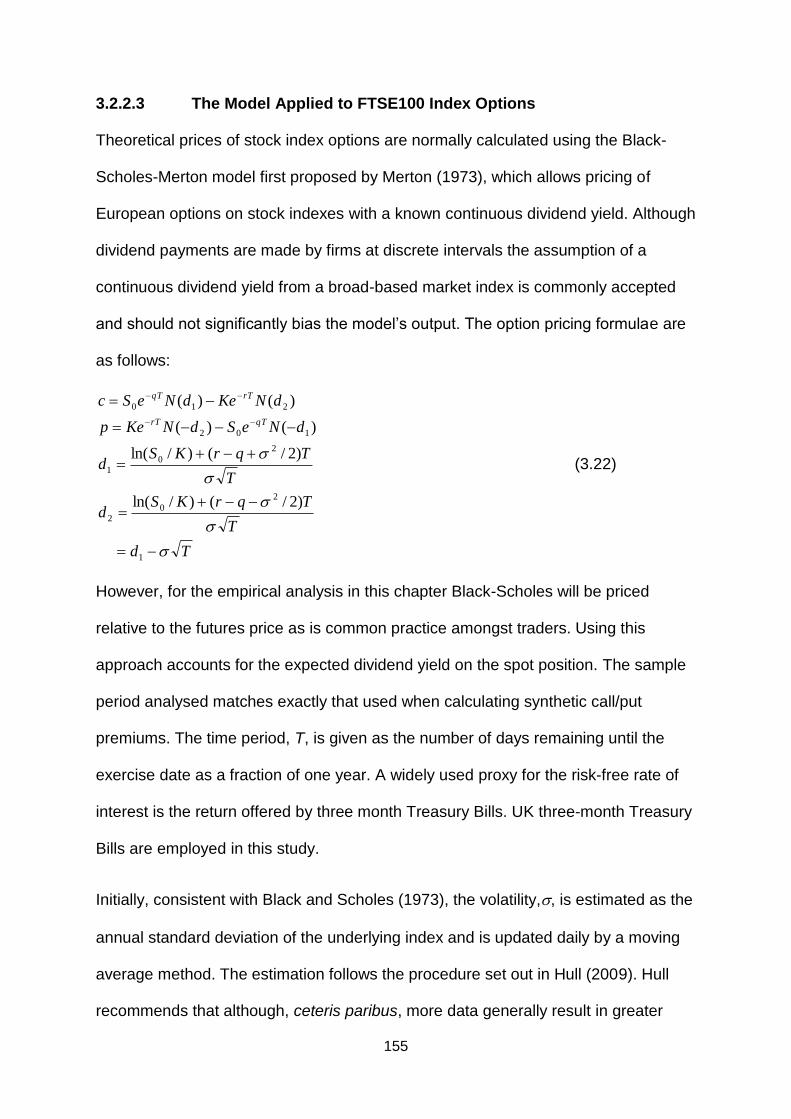
155

3.2.2.3 The Model Applied to FTSE100 Index Options

Theoretical prices of stock index options are normally calculated using the Black-

Scholes-Merton model first proposed by Merton (1973), which allows pricing of

European options on stock indexes with a known continuous dividend yield. Although

dividend payments are made by firms at discrete intervals the assumption of a

continuous dividend yield from a broad-based market index is commonly accepted

and should not significantly bias the model‟s output. The option pricing formulae are

as follows:

Td

T

TqrKSd

T

TqrKSd

dNeSdNKep

dNKedNeSc

qTrT

rTqT

1

2

0

2

2

0

1

102

210

)2/()/ln(

)2/()/ln(

)()(

)()(

(3.22)

However, for the empirical analysis in this chapter Black-Scholes will be priced

relative to the futures price as is common practice amongst traders. Using this

approach accounts for the expected dividend yield on the spot position. The sample

period analysed matches exactly that used when calculating synthetic call/put

premiums. The time period, T, is given as the number of days remaining until the

exercise date as a fraction of one year. A widely used proxy for the risk-free rate of

interest is the return offered by three month Treasury Bills. UK three-month Treasury

Bills are employed in this study.

Initially, consistent with Black and Scholes (1973), the volatility,, is estimated as the

annual standard deviation of the underlying index and is updated daily by a moving

average method. The estimation follows the procedure set out in Hull (2009). Hull

recommends that although, ceteris paribus, more data generally result in greater

156

accuracy, volatility does change over time and older data may have little relevance in

predicting the future. It is suggested that a time window of 90-180 days is

appropriate, with the number of observations, n, set to match the length of time

remaining until the option matures. In the case of this study the options are relatively

close to maturity and hence, for the purposes of computing each volatility estimate, n

is set to 90 days. For example, the January 2000 contracts matured on 21st January.

The volatility used to price these contracts on 1st November 1999 will be computed

from returns on the FTSE100 for the 90 days prior to that date. Following Fama

(1965) and French (1980) trading days will be used to estimate volatility. Thus

annual volatility will be calculated as volatility per trading day multiplied by 252 .

Volatility per trading day is computed in accordance with equations (3.23) and (3.24).

1

lni

ii S

Su (3.23)

2

11

2

1

1

1

1

n

i

i

n

i

i unn

un

s (3.24)

One of the main problems with testing the Black-Scholes model has been the

selection of an appropriate measure of volatility. As volatility is the only directly

unobservable input into the Black-Scholes equation it is probable that many pricing

errors occur as a result of incorrectly estimating the volatility of the underlying asset.

An appropriate robustness test would be to estimate Black-Scholes prices using

alternative volatility measures. Possible alternative volatility updating schemes that

157

could be employed are the exponentially weighted moving average (EWMA) or the

GARCH (1,1)17.

The EWMA model presented in equation (3.25) is employed with a value of λ = 0.94.

This is consistent with J.P. Morgan‟s RiskMetrics database. According to Hull (2009),

J.P. Morgan‟s RiskMetrics Monitor (1995) asserts that a λ value of 0.94 gives

estimates of volatility that provide the closest match to realised volatility.

2

1

2

1

2 1 nnn u (3.25)

Moving average daily volatilities are calculated using 252 daily observations and

converted to annual volatilities.

The GARCH(1,1) model presented in equation (3.26) is employed for volatility

updating using parameters produced by maximum likelihood estimation.

2

1

2

1

2

nnn u (3.26)

where

LV

Intuitively, using daily data a GARCH(1,1) models today‟s estimate of volatility

squared as a weighted average of the long-run variance rate, yesterday‟s market

return squared and yesterday‟s volatility forecast.

The GARCH(1,1) model may improve upon the EWMA as it gives some weight to

the long-run average variance rate thus allowing for mean reversion as well as

17

The GARCH estimation employed here is not to be confused with the GARCH option pricing models

proposed by Duan (1995), Heston and Nandi (1999) or Ritchken and Trevor (1999). In this study EWMA and

GARCH are merely being employed to forecast the volatility parameter for a Black-Scholes framework.

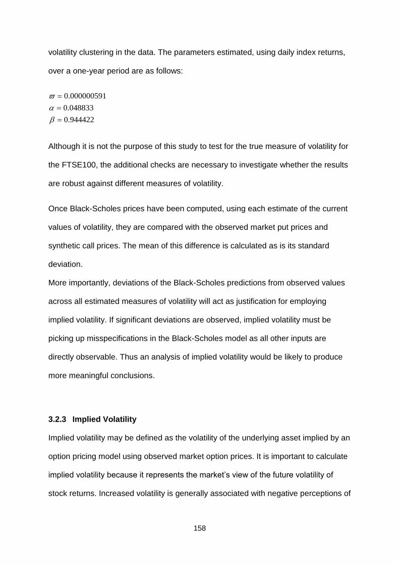
158

volatility clustering in the data. The parameters estimated, using daily index returns,

over a one-year period are as follows:

944422.0

048833.0

000000591.0

Although it is not the purpose of this study to test for the true measure of volatility for

the FTSE100, the additional checks are necessary to investigate whether the results

are robust against different measures of volatility.

Once Black-Scholes prices have been computed, using each estimate of the current

values of volatility, they are compared with the observed market put prices and

synthetic call prices. The mean of this difference is calculated as is its standard

deviation.

More importantly, deviations of the Black-Scholes predictions from observed values

across all estimated measures of volatility will act as justification for employing

implied volatility. If significant deviations are observed, implied volatility must be

picking up misspecifications in the Black-Scholes model as all other inputs are

directly observable. Thus an analysis of implied volatility would be likely to produce

more meaningful conclusions.

3.2.3 Implied Volatility

Implied volatility may be defined as the volatility of the underlying asset implied by an

option pricing model using observed market option prices. It is important to calculate

implied volatility because it represents the market‟s view of the future volatility of

stock returns. Increased volatility is generally associated with negative perceptions of

159

the future movements in the aggregate stock market and is hence a useful indicator

of crash expectations. It should be possible to construct a time series of implied

volatility which is indicative of consensus among traders‟ estimates of changing

volatility before and during the bear market at the turn of the century. Justification for

the analysis of implied volatility is provided by Chiras and Manaster (1978). They

employed data from the Chicago Board Options Exchange to compute implied

volatility. The explanatory power of the implied volatility was then compared with that

of historical volatility with the result that the former was found to provide much better

estimates of future volatility. This suggests that traders have access to, and are

using, more than simply historical data to form their expectations. Implied volatilities

are based on current prices and would therefore be expected to have future

expectations impounded in them. Gemmill (1996) argued that implied volatility is

preferable to prices when calculating skewness for a number of reasons. Firstly, as

option prices are almost linear in volatility there should be very little difference in the

behaviour of an implied volatility-based and a price-based measure of skewness.

Second, the volatility-based measure has the advantage that, unlike prices, volatility

is not sensitive to maturity. Gemmill asserts that this should make the volatility-based

measure less prone to sampling error. A further advantage is a consistency with

market practice in that traders talk in terms of volatility as opposed to price smiles.

Gemmill and Saflekos (2000) assert that traders price options using a Black-Scholes

model but with different levels of volatility applied to each exercise price, resulting in

a volatility smile. They would then apply the volatility smile from day t-1 to compute

the prices of options on day t. This is clearly inconsistent with the theoretical model

in which volatility is assumed to be constant across all exercise prices. In addition,

MacBeth and Merville (1979) note that, for individual equities, implied volatilities are

160

higher for in-the-money than for out-of-the-money contracts. This finding contradicts

that of Black (1975) who finds the opposite result. Furthermore, Merton (1976) found

implied volatilities that were high for both deep in- and out-of-the-money options. The

one obvious conclusion to draw from these results is that there is variability in the

market‟s expectation of the volatility of the underlying asset over time.

It is important to exercise caution by recognising some of the weaknesses in the

predictive power of implied volatility. For example, Canina and Figlewski (1993)

analysed the predictive power of implied volatility extracted from S&P 100 options.

They examine returns on the S&P 100 index between 1983 and 1987 and discover

that the implied volatility forecasts are biased. Furthermore Canina and Figlewski do

not find statistically significant forecasting power. However Christensen and

Prabhala (1998) adjust Canina and Figlewski‟s methodology and extend the sample

period by 8 years to find implied volatility which is unbiased and has statistically

significant forecasting power.

Once implied volatilities have been calculated they may then be displayed

graphically as a volatility smile or skew. Further and more in-depth analysis of

literature in this area will be presented in relation to implied volatility indexes in

Chapter 4.

Implied volatility needs to be calculated using an iterative procedure such as that

used by the solver add-in in Microsoft Excel. The package chooses alternative

values of implied volatility so as to minimise

2ˆ cc

where

c theoretical (B-S) premium

c = quoted call premium

161

The purpose of calculating implied volatilities of put and synthetic call options is to

determine if the implied volatility of the former exceeds that of the latter. Also the

intertemporal magnitude of this relationship is of interest, based on the assumption

that there is a usual degree of skewness.

The Black-Scholes model gives rise to the expectation that implied volatility will be

constant across puts and calls and also across exercise prices. In other words the

volatility smile will be flat. The market view of the volatility of the underlying asset at

a particular point should not change simply because a different class of derivative is

being priced. However there may be an expectation of observing differing volatilities

for puts and calls asymmetrically distributed around the spot price. Differing implied

volatilities for different degrees of „moneyness‟ within an option type is evidence of a

symmetric or asymmetric volatility smile (or skew) which is not flat. Evidence of such

a pattern of implied volatility suggests some type of inaccuracy in the Black-Scholes

model. In particular, the Black-Scholes model is objective in that it does not provide

for investor sentiment or the pricing of jump risk. However, the purpose of this study

is not to test the validity of the pricing model, rather the intention is to identify

evidence of traders‟ expectations and if those expectations are fulfilled. Further,

volatility smiles and skews may correspond to negatively skewed implied probability

distributions.

Implied volatilities for each contract are calculated for both put and synthetic call

contracts and their development over time is studied. The relative implied volatilities

can then be compared by calculating a percentage difference for each contract on

each day. A mean value of percentage difference in implied volatility is then

produced for each degree of „moneyness‟ of a particular contract. A positive value

162

indicates greater implied volatility in puts whereas a negative value indicates greater

implied volatility in calls.

163

3.3 Data

Aggregate end-of-day values for the FTSE100 index, FTSE100 futures price and

rates of return on UK 3-month Treasury bills are collected from Datastream. These

are consistent with data on the associated European style index options contract

listed on the London International Financial Futures Exchange (LIFFE)18. Owing to

the relatively low option trading volume during the period of analysis the options

selected are those closest to maturity as these contracts account for the bulk of the

trading volume. Options with a variety of maturities will be examined in Chapter 6 in

relation to momentum and overreaction tests. The data employed in Chapter 6 is

sampled over a more recent period and is associated with higher trading volume of

FTSE100 index options. The average moneyness of each series of put call pairs is

given in Table 3.0. Moneyness is defined as the exercise price divided by the

forward price. These values are consistent with out-of-the-money puts. The

moneyness of a call in a matched pair will be approximated by the reciprocal.

Table 3.0 Average Moneyness of Series of Option Pairs

Series Title CP1 CP2 CP3 CP4

K/F 0.994448 0.986345 0.978242 0.970139

18

Options data is purchased from LIFFE Euronext Online. The options selected expire on the third Friday of the

delivery month or the preceding Thursday if the Friday is a public holiday.

164

Although some studies employ the LIBOR as the risk free rate for option pricing the

selection of rate is of little importance due to the relative insensitivity of option price

to this parameter as asserted by Macbeth and Merville (1979). Furthermore, Black

(1989) has noted that, in general, it is volatility rather than interest rates that has the

most significant impact on option prices.

The data collected begin from 1st June 1998 continuing up to, and including 30th June

2002. This allows examination of the period prior to and during the recent bear

market and allows comparison of expectations across a range of different time

periods.

Figure 3.1 illustrates the level of the index underlying the options contracts over the

period 1st June 1998 to 12th September 2003. It can be clearly observed that the

FTSE100 index peaked at the beginning of January 2000. However, it must be noted

that the downturn was initially gradual with some sustained periods of stability. One

would expect that there would be little initial impact upon investor expectations

simply because there is only a very small change over the first twelve months. This

may be regarded as short-run fluctuations which would not appear to be indicative of

a long-run trend. However, from the beginning of 2001 the downturn gains

momentum and, if traders are already bearish, this should be more likely to have a

significant impact on their expectations. Or more precisely, it should increase the

likelihood of them implementing protective put strategies. This in itself would not

necessarily indicate any inefficiency in the market, rather it would be consistent with

traders adjusting their expectations in response to the arrival of new information. For

any inefficiency to exist it needs to be shown that traders are able to identify a period

of falling prices prior to those price falls occurring.

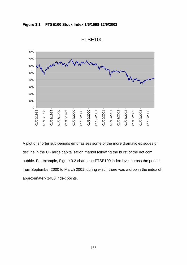
165

Figure 3.1 FTSE100 Stock Index 1/6/1998-12/9/2003

A plot of shorter sub-periods emphasises some of the more dramatic episodes of

decline in the UK large capitalisation market following the burst of the dot com

bubble. For example, Figure 3.2 charts the FTSE100 index level across the period

from September 2000 to March 2001, during which there was a drop in the index of

approximately 1400 index points.

0

1000

2000

3000

4000

5000

6000

7000

8000

01

/06

/199

8

01

/10

/199

8

01

/02

/199

9

01

/06

/199

9

01

/10

/199

9

01

/02

/200

0

01

/06

/200

0

01

/10

/200

0

01

/02

/200

1

01

/06

/200

1

01

/10

/200

1

01

/02

/200

2

01

/06

/200

2

01

/10

/200

2

01

/02

/200

3

01

/06

/200

3

FTSE100

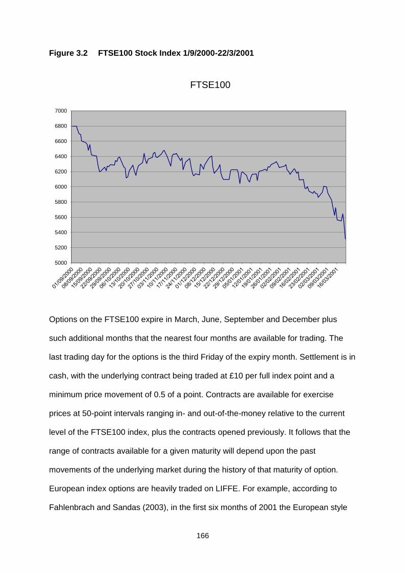
166


Options on the FTSE100 expire in March, June, September and December plus

such additional months that the nearest four months are available for trading. The

last trading day for the options is the third Friday of the expiry month. Settlement is in

cash, with the underlying contract being traded at £10 per full index point and a

minimum price movement of 0.5 of a point. Contracts are available for exercise

prices at 50-point intervals ranging in- and out-of-the-money relative to the current

level of the FTSE100 index, plus the contracts opened previously. It follows that the

range of contracts available for a given maturity will depend upon the past

movements of the underlying market during the history of that maturity of option.

European index options are heavily traded on LIFFE. For example, according to

Fahlenbrach and Sandas (2003), in the first six months of 2001 the European style

5000

5200

5400

5600

5800

6000

6200

6400

6600

6800

7000

FTSE100

167

FTSE 100 index option contract had an average monthly volume of 1.25 million

contracts and an average monthly open interest of over 1.4 million contracts.

Initially tests were performed on closing put and call premiums from 1st November

1999 to 10th December 1999 for European style contracts due to expire in January

2000. This is the first contract to expire after the FTSE100 peaked on 3rd January

2000.

Consistent with Bates (1991), the sample excludes contracts with maturity in excess

of 118 days and less than 28 days. Longer maturity contracts are too thinly traded

and those of shorter maturity too close to expiration, and hence information may be

obscured by the associated market activity, to provide reliable indicators of crash

expectations. Moreover, Heston (1993) argues that very short term options have

substantial time decay that could interfere with the ability to isolate the volatility

parameters, and very long term options are simply not actively traded.

End of day prices at four strike prices for calls and four strike prices for puts are used

in order to ensure a reasonably wide „moneyness‟ range. Again, contracts further

out-of-the-money are considered to be too thinly traded to provide reliable

information. In the case of FTSE100 options, many contracts outside of the selected

moneyness range are not traded at all during the sample period.

End-of-day data should be sufficiently frequent in order to analyse investor sentiment

because, if crash expectations persist over a lengthy time period, it is unlikely that

significant information will be revealed by the pattern on a single day other than

perhaps the day prior to the onset of a crash. However the bear market that began in

2000 was gradual and the data is unlikely to exhibit anything as dramatic as the

crash of 1987 for example.

168

As options are only available for specific exercise prices determined by the

exchange, the exercise prices of out-of-the-money puts and calls will be

asymmetrically distributed around the value of the underlying index. For example, on

the 1st November 1999 the FTSE100 closed at 6284. On the same date there was

also a call option with strike price 6325. That is, forty-one index points out-of-the-

money. However there was no exchange-traded put option with a strike price of

6243. The nearest out-of-the-money contract to the spot price had a strike of 6275.

Clearly this means that any comparison between put and call premiums will reflect

not only crash expectations but also the differing degrees of „moneyness.‟

To address this problem an iterative interpolation process is employed in order to

produce option prices distributed symmetrically around the index value. This process

is used to adjust call prices to create what will be referred to as a „synthetic call

premium‟. This follows the procedure adopted by Gemmill (1996) who uses linear

interpolation to produce implied volatilities of options with strike prices 2% away from

the forward price.

All options used are European style thus avoiding the problem of any early exercise

premium associated with American options.

169

3.4 Results and Analysis

3.4.1 Call/Put Premiums

The results presented in Table 3.1 are based on the prices of options that expire on

the third Friday of the delivery month. The expiry month for each contract is given in

the first column of the table. Call/put premiums, or skewness measures, of out-of-

the-money options with exercise prices evenly distributed around the forward price

are presented. Synthetic call/put pairs are matched in terms of moneyness and

maturity. The moneyness range, CP1 to CP4 is defined in Table 3.0. For consistency

each monthly series is sampled at the end of each of the 30 trading days prior to the

final 30 days of trading. Thus the sample period is T-60 to T-30, where T is the

expiry date and only trading days are counted.

Table 3.1 Mean Synthetic Call/Put Skewness Measure

Contact Expiry January 2000 – June 2002

( )

Expiry

N CP1 CP2 CP3 CP4

January 2000 30 -0.038451***

(4.413933)

-0.00519

(-0.61286)

-0.05342***

(-5.87339)

-0.11351***

(-11.2141)

March 2000 30 -0.09721***

(-10.6153)

-0.13214***

(-14.2787)

-0.17069***

(-17.4542)

-0.21374***

(-21.4929)

June 2000 30 -0.11356***

(-8.74182)

-0.14355***

(-10.9059)

-0.17681***

(-13.2547)

-0.2195***

(-15.5118)

September 2000 30 -0.10878***

(-8.1671)

-0.1393***

(-10.1632)

-0.17341***

(-11.8888)

-0.21328***

(-13.4478)

December 2000 30 -0.1852***

(-26.0485)

-0.21749***

(-29.1955)

-0.25319***

(-31.3221)

-0.2933***

(-32.5510)

March 2001 30 -0.2028***

(-69.552)

-0.23882***

(-74.8194)

-0.27956***

(-66.5500)

-0.3247***

(-56.1617)

170

June 2001 30 -0.1736***

(-42.1105)

-0.20771***

(-38.4579)

-0.24731***

(-34.7471)

-0.2941***

(-30.6061)

September 2001 30 -0.15357

(-54.5713)***

-0.18787

(-57.5087)

-0.2287

(-57.2304)

-0.27675

(-52.9571)

June 2002 30 -0.11893***

(-11.6009)

-0.17351**

(-16.4031)

-0.2360***

(-20.7238)

-0.30522***

(-23.2497)

Numbers in parentheses are t-statistics. *** significant at the 1% level, ** significant at the 5% level. Critical values are 2.462 and 2.045 respectively.

The results presented in Table 3.1 are all negative and, apart from the second out-

of-the-money series maturing in January 2000, are all significant. This is consistent

with a „usual‟ situation of puts priced highly relative calls matched by moneyness and

maturity. The most notable feature of the results is the shift in both the size and

significance of the skewness measure that occurs between observations on the

contracts maturing in September and December 2000. The FTSE100 fell by less

than 0.5% in the period between the observation mid-points of the two series.

However the index fell by 3.78% between the expiry dates of the respective option

contracts. This finding is consistent with a strong perception of downside risk

amongst option traders towards the end of 2000.

The smallest and least significant values of the skewness measure relate to values

of the January maturity option pair from prices in November and December 1999.

This may be interpreted as the highest level of trader optimism throughout the

sample period. The value of the skewness measure increases consistently for the

March, June and September maturity contracts prior to the major shift.

With regard to moneyness the expensiveness of puts relative to calls increases as

options are observed further out-of-the-money. This provides support to the findings

of Rubinstein (1994) and Chen, Hong and Stein (2001) that traders are concerned

171

about the possibility of a downturn and weight this more highly than the possibility of

an upturn. They then price put and call options to accord with these concerns.

The move from the January to the March contract also coincides with a shift in the

size and significance of the synthetic call/put skewness measure. Although this shift

is not of the magnitude of that observed later in the year it is noteworthy as it

coincides with the onset of the downturn. Observations on this contract run through

January up to the 14th of February 2000. Out-of-the-money put premiums have

clearly increased, compared to observations on the preceding contract, relative to

those of the corresponding out-of-the-money synthetic call premiums during this

period. This result may be interpreted as traders becoming more pessimistic about

future market moves. The large negative figure for the deepest out-of-the-money

options suggests that traders believe that a large market downturn is considerably

more likely than an upturn of similar magnitude. This pricing behaviour is consistent

with aversion to extreme losses.

The results for the remainder of the period show a steady decline in the value of the

skewness measure for options near the money. However, for the deepest out-of-the-

money options the value of the skewness measure remains consistently high. As the

prices of deepest out-of-the-money options hold the greatest amount of information

(for example see Pan and Poteshman, 2006), they provide important insights into the

expectations of investors. As all of these values are negative and significant, with a

mean value of -0.2988 for the December 2000 through September 2001 contracts, it

can be inferred that options investor expectations were bearish throughout this

period.

A notable feature of Figure 3.1 is a data „spike‟ and high level of market turbulence

around the time of the events of September 2001. Option premiums could not be

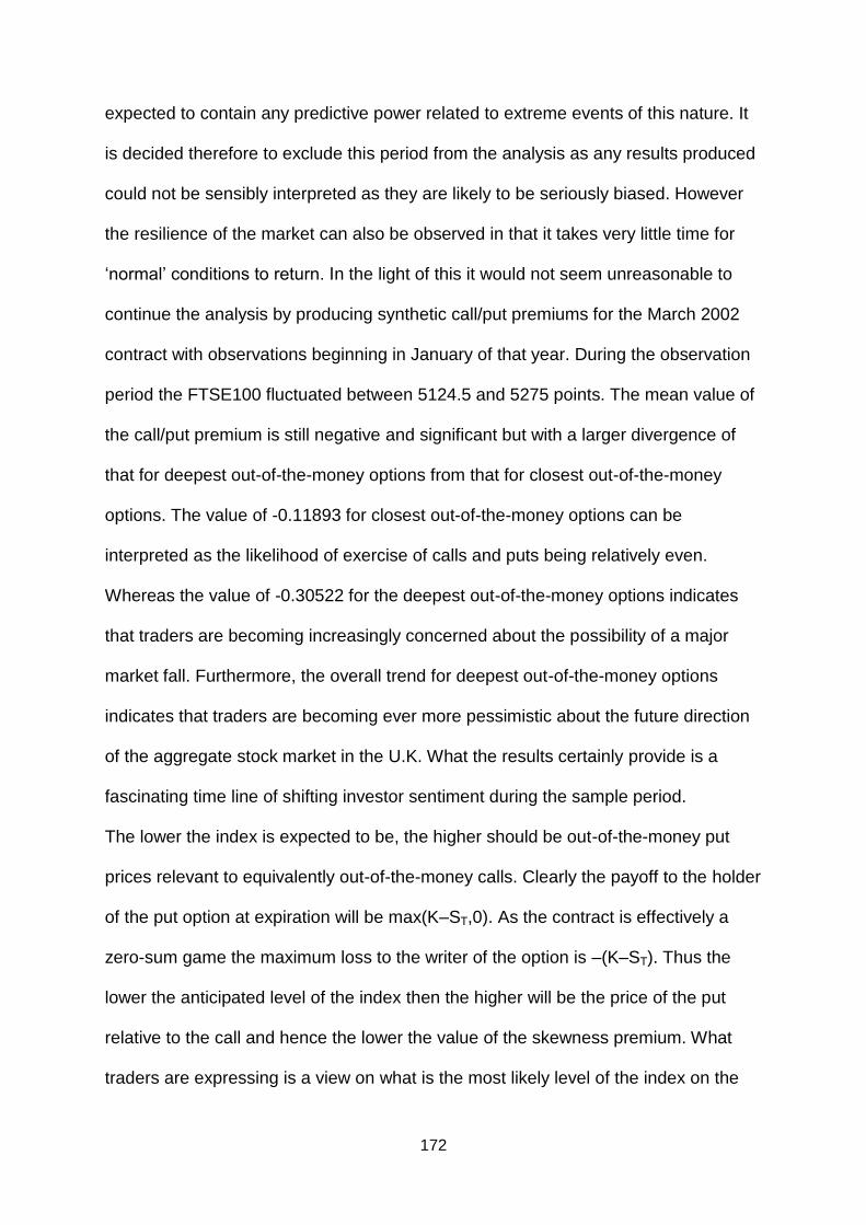
172

expected to contain any predictive power related to extreme events of this nature. It

is decided therefore to exclude this period from the analysis as any results produced

could not be sensibly interpreted as they are likely to be seriously biased. However

the resilience of the market can also be observed in that it takes very little time for

„normal‟ conditions to return. In the light of this it would not seem unreasonable to

continue the analysis by producing synthetic call/put premiums for the March 2002

contract with observations beginning in January of that year. During the observation

period the FTSE100 fluctuated between 5124.5 and 5275 points. The mean value of

the call/put premium is still negative and significant but with a larger divergence of

that for deepest out-of-the-money options from that for closest out-of-the-money

options. The value of -0.11893 for closest out-of-the-money options can be

interpreted as the likelihood of exercise of calls and puts being relatively even.

Whereas the value of -0.30522 for the deepest out-of-the-money options indicates

that traders are becoming increasingly concerned about the possibility of a major

market fall. Furthermore, the overall trend for deepest out-of-the-money options

indicates that traders are becoming ever more pessimistic about the future direction

of the aggregate stock market in the U.K. What the results certainly provide is a

fascinating time line of shifting investor sentiment during the sample period.

The lower the index is expected to be, the higher should be out-of-the-money put

prices relevant to equivalently out-of-the-money calls. Clearly the payoff to the holder

of the put option at expiration will be max(K–ST,0). As the contract is effectively a

zero-sum game the maximum loss to the writer of the option is –(K–ST). Thus the

lower the anticipated level of the index then the higher will be the price of the put

relative to the call and hence the lower the value of the skewness premium. What

traders are expressing is a view on what is the most likely level of the index on the

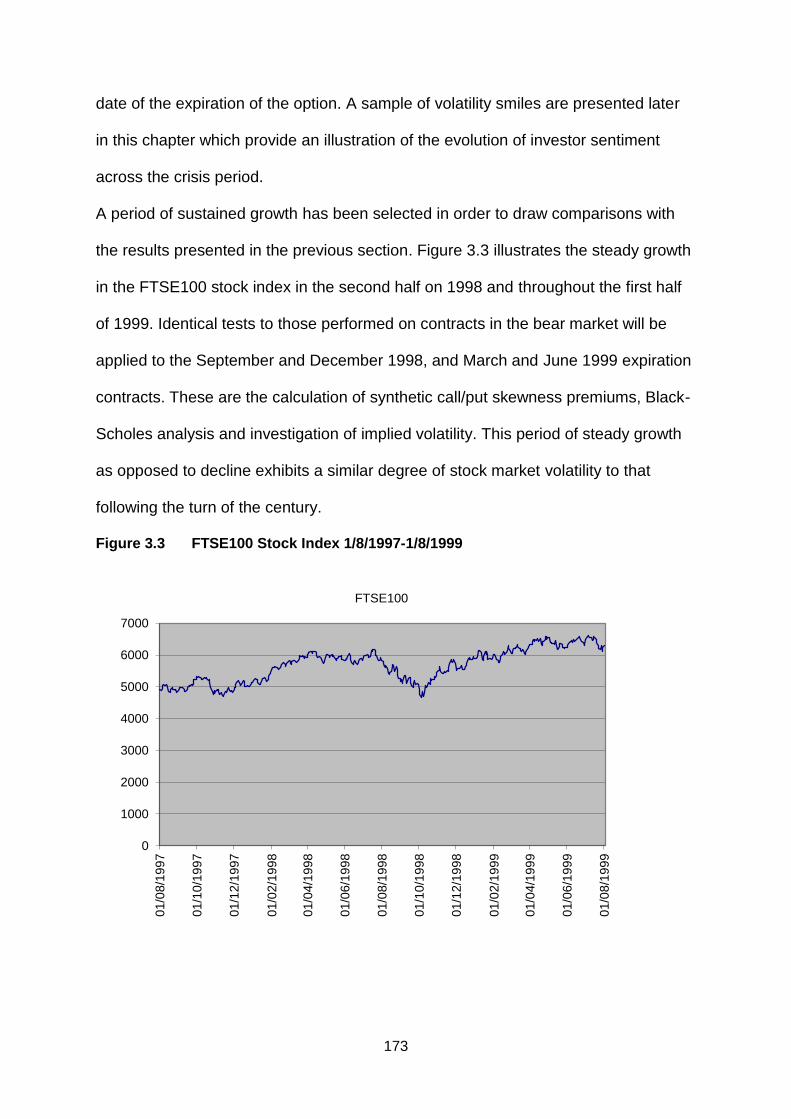
173

date of the expiration of the option. A sample of volatility smiles are presented later

in this chapter which provide an illustration of the evolution of investor sentiment

across the crisis period.

A period of sustained growth has been selected in order to draw comparisons with

the results presented in the previous section. Figure 3.3 illustrates the steady growth

in the FTSE100 stock index in the second half on 1998 and throughout the first half

of 1999. Identical tests to those performed on contracts in the bear market will be

applied to the September and December 1998, and March and June 1999 expiration

contracts. These are the calculation of synthetic call/put skewness premiums, Black-

Scholes analysis and investigation of implied volatility. This period of steady growth

as opposed to decline exhibits a similar degree of stock market volatility to that

following the turn of the century.


0

1000

2000

3000

4000

5000

6000

7000

01

/08

/19

97

01

/10

/19

97

01

/12

/19

97

01

/02

/19

98

01/0

4/1

998

01

/06

/19

98

01

/08

/19

98

01

/10

/19

98

01

/12

/19

98

01

/02

/19

99

01

/04

/19

99

01

/06

/19

99

01

/08

/19

99

FTSE100

174

Mean synthetic call/put skewness measures are presented in Table 3.2.

Table 3.2 Mean Synthetic Call/Put Skewness Measure

Contract Expiry September 1998 – June 1999

Expiry Observations CP1 CP2 CP3 CP4

September

1998

30 -0.2404

(-44.8016)

-0.27107

(-45.7967)

-0.30851

(-51.8877)

-0.35344

(0.034334)

December

1998

30 -0.14712

(-35.3770)

-0.18131

(-35.6990)

-0.21899

(-34.5475)

-0.26135

(-37.3776)

March

1999

30 -0.11203

(-47.3799)

-0.1396

(-55.8871)

-0.16929

(-49.9947)

-0.1994

(-45.6029)

June

1999

30 -0.18781

(-51.2229)

-0.18781

(-51.2229)

-0.22816

(-58.7345)

-0.2723

(-58.4907)

Figures in parentheses are t-statistics.

All of the skewness measures contained in Table 3.2 are negative and significant

indicating that FTSE100 put options remain expensive relative to corresponding calls

for each degree of moneyness.

The first row of observations contained in Table 3.2 relate to the period July 1st to

August 11th 1998. During this period the FTSE100 fluctuated between 5435 and

6222 points. A notable feature of the results is that out-of-the-money puts are still

expensive relative to out-of-the-money calls despite the general trend of the

aggregate UK stock market in 1998 being upward. Furthermore, the relationship

becomes more pronounced according to how far out-of-the-money the series is. This

finding poses a number of questions:

(i) Do the data suggest that market participants are pessimistic at this point in

time? This, in itself, would not be a violation of market efficiency.

(ii) Is there a detectable pattern in the relationship between put and call

options and hence a violation of market efficiency? That is, if the

175

relationship between equally out-of-the-money puts and calls consistently

predicts aggregate market moves, such predictability contradicts the weak

form of the efficient markets hypothesis.

(iii) Are investors becoming more optimistic but, perhaps because of

anchoring and/ or conservatism, this optimism is subject to a lag? This

would also contradict market efficiency.

(iv) Are the data merely demonstrating a persistent relationship between the

relative premiums of out-of-the-money puts and calls? If this were the case

then there would be no repeating patterns in prices that could be exploited

by arbitrageurs. Hence, at most this would represent a technical

inefficiency.

In an attempt to address these questions the results for the next three contracts

under investigation are presented in the next three rows of Table 3.2.

The second row of observations relate to the period October 1st to November 11th

1998. During this period the FTSE100 fluctuated between 4699 and 5664 points.

Although the aggregate market dipped during this period, as can be observed on

Figure 3.2, the pattern of the mean call/put premium displayed in Table 3.2 is very

similar to that for the September contract. Thus it is difficult to draw any further

inferences. The third and fourth rows of observations relate to the period from

January 4th to February 12th 1999 and April 1st to May14th 1999 respectively. During

this period the FTSE100 fluctuated between 5765 and 6635 points. With reference to

the questions posed earlier:

(i) Overall it would appear that traders remained concerned about the

possibility of a market decline as puts are consistently expensive relative

to calls.

176

(ii) It is not possible to confidently infer market predictability from these

results.

(iii) It may be that traders are slowly becoming more optimistic, however it

seems that pessimistic expectations persist within risk-averse traders

alongside aversion to extreme losses.

3.4.2 Black-Scholes Prices

The Black-Scholes model, using the relevant futures contract as the underlying

asset, is employed to price FTSE100 index options. The null hypothesis is that there

will be no significant difference between the Black-Scholes price and the market

price. The alternative hypothesis is that the Black-Scholes model will produce

systematic and significantly different prices to those observed in the market. The

model is estimated using standard deviation as the traditional measure of volatility.

However, as a robustness check, volatility is also estimated using an EWMA and

GARCH(1,1) model which allow for time varying volatility. Rejection of the null

hypothesis motivates the analysis of implied volatility for further tests, as the volatility

parameter will be picking up other influences, such as investor expectations, not

included in the specification of the model.

The reported statistics are numbered by moneyness, M, which runs from 1 to 4 and

have the same values as presented in table 3.0 corresponding to CP1 to CP4.

Hence these denote, for each contract, the nearest to fourth nearest out-of-the-

money options respectively. The mean statistic in column four, in each case, tells us

the mean value, over the sample period for a particular contract, of the observed (or

synthetic) option price minus the theoretical Black-Scholes price. If the value is

177

positive then the Black-Scholes model is underpricing the option, and if negative the

model is overpricing the option.

The Black-Scholes analysis generates some interesting results. The first notable

feature is the divergence of the theoretical call price from the observed price. In

order to verify that this finding was not simply attributable to the method used to

calculate synthetic call premiums the same calculations were applied to actual out of

the money call contracts. On average the percentage divergence of the actual call

price from the Black-Scholes price was found to be at least as large as was found

when using synthetic calls.

178

Table 3.3 Percentage Deviation of Theoretical Black-Scholes-Merton Price from Synthetic Call Premium and Actual Put Premium 2000

Maturity M Contract Mean Pricing Error

Standard Deviation

EWMA GARCH

Jan 1 Call -0.10316*** (-10.7547)

-0.01038 (-1.27485)

-0.01606* (-2.09031)

Put 0.251308*** (16.20808)

0.475771*** (26.28433)

0.459719*** (29.81945)

2 Call -0.12603*** (-11.9435)

-0.02122** (-2.30409)

-0.02783*** (-3.22064)

Put 0.295601*** (17.05338)

0.572783*** (26.20732)

0.553062*** (29.83999)

3 Call -0.15154*** (-13.4329)

-0.03426*** (-3.46688)

-0.04186*** (-4.56952)

Put 0.372214*** (19.49185)

0.694381*** (26.43539)

0.669971*** (30.3943)

4 Call -0.18195*** (-14.7245)

-0.05224*** (-4.67709)

-0.06089*** (-5.90646)

Put 0.488826*** (23.18965)

0.842336*** (26.67895)

0.811952*** (31.02001)

Mar 1 Call 0.004494 (0.377577)

-0.06462*** (-2.30244)

-0.04329* (-1.74649)

Put 0.884263*** (28.38101)

0.707325*** (6.054117)

0.759051*** (7.835681)

2 Call 0.004294 (0.325414)

-0.07242** (-2.20215)

-0.049** (-1.69909)

Put 1.039308*** (29.25237)

0.838331*** (5.701576)

0.895404*** (7.442147)

3 Call 0.001931

(0.133739)

-0.08211**

(-2.13396)

-0.05673** (-1.69503)

Put 1.223234***

(29.53575)

0.997892***

(5.313873)

1.05945*** (6.989161)

4 Call 0.001363

(0.084821)

-0.09013**

(-2.01395)

-0.06287* (-1.62843)

Put 1.452179***

(30.5598)

1.201166***

(4.964374)

1.265934*** (6.585095)

Jun 1 Call -0.1712***

(-8.95433)

-0.17916***

(-8.86636)

-0.16614*** (-7.61992)

Put 0.367675***

(9.318349)

0.347601***

(7.789321)

0.436964*** (8.839514)

2 Call -0.1885***

(-8.90713)

-0.19701***

(-8.78896)

-0.18195*** (-7.5991)

Put 0.419902***

(9.388686)

0.397728***

(7.821245)

0.498969*** (8.911336)

3 Call -0.20739***

(-9.00197)

-0.21642***

(-8.84255)

-0.19924*** (7.67228)

Put 0.484862***

(9.623212)

0.460472***

(7.958929)

0.575825*** (9.086265)

4 Call -0.2301***

(-9.09137)

-0.2396***

(-8.9133)

-0.22036*** (-7.77512)

Put 0.562755***

(9.930322)

0.535744***

(8.15939)

0.667974*** (9.307021)

Sep 1 Call -0.36441** -0.23746*** -0.24496***

179

(-48.8095) (-38.8074) (-45.4197)

Put 0.175372***

(20.42252)

0.800301***

(15.19505)

0.744521*** (18.78662)

2 Call -0.39771***

(-45.5732)

-0.25444***

(-37.6116)

-0.26361*** (-44.5011)

Put 0.184841***

(18.27696)

0.932832***

(14.09144)

0.860127*** (17.49945)

3 Call -0.4339***

(-44.3994)

-0.27429***

(-36.7682)

-0.2853*** (-44.1446)

Put 0.199645***

(16.2697)

1.100709***

(12.94113)

1.005273*** (16.05732)

4 Call -0.46706***

(-43.9061)

-0.2883***

(-22.9661)

-0.30177*** (-28.2244)

Put 0.222192***

(14.8082)

1.315972***

(12.03028)

1.189654*** (14.95187)

Dec 1 Call -0.06144***

(-3.21202)

-0.03508*

(-1.47214)

-0.02951 (-1.26421)

Put 0.624373***

(13.13467)

0.81879***

(13.80338)

0.834038*** (14.95094)

2 Call -0.06627***

(-2.95612)

-0.03148

(-1.08143)

-0.02515 (-0.91865)

Put 0.727549***

(13.34351)

0.967036***

(13.62529)

0.985076*** (14.86255)

3 Call -0.07564***

(-2.9793)

-0.0315

(-0.94349)

-0.02439 (-0.78272)

Put 0.85732***

(13.36909)

1.154763***

(13.32945)

1.176195*** (14.60699)

4 Call -0.08605***

(-2.95483)

-0.03118

(-0.7982)

-0.02331 (-0.64729)

Put 1.018337***

(13.57769)

1.391077***

(13.142)

1.416613*** (14.49322)

Figures in parentheses are t-statistics. The relevant 1%, 5% and 10% critical values

are 2.462, 1.699 and 1.311 respectively.

Most of the percentage deviations presented in Table 3.3 are significant at the 1%

level indicating that the Black Scholes price is consistently different to the market

price across call and put options. The relationship is also robust to the measure of

volatility.

It is clear from the results presented in Table 3.3 that the Black-Scholes model

consistently underprices FTSE100 put options and consistently overprices the

corresponding calls. In general, there is a significant deviation of the observed price

from the theoretical price.

180



Standard Deviation

EWMA GARCH

Mar 1 Call -0.22485*** (-10.0131)

-0.20051*** (-13.9985)

-0.19631*** (-12.4128)

Put 0.365665*** (8.7304)

0.454519*** (16.32939)

0.46278*** (16.57386)

2 Call -0.25119*** (-9.97842)

-0.22327*** (-14.0076)

-0.21881*** (-12.3959)

Put 0.422698*** (8.535601)

0.531994*** (15.9558)

0.54054*** (16.3128)

3 Call -0.27856*** (-9.95092)

-0.24719*** (-14.0009)

-0.24245** (-12.3626)

Put 0.4935*** (8.515349)

0.629576*** (15.34685)

0.637888*** (16.0083)

4 Call -0.3086*** (-10.0855)

-0.27419*** (-14.3052)

-0.26915*** (-12.5862)

Put 0.580873*** (8.583309)

0.750963*** (14.98669)

0.758451*** (15.98649)

Jun 1 Call -0.24173*** (-8.6783)

-0.34884*** (-30.4796)

-0.32512*** (-24.2798)

Put 0.117085*** (3.195552)

-0.08531*** (-8.27877)

-0.04147*** (-3.52642)

2 Call -0.2737*** (-8.82722)

-0.38921*** (-30.0424)

-0.36419*** (-24.148)

Put 0.13721*** (3.210466)

-0.0915*** (-7.84735)

-0.04299*** (-3.15489)

3 Call -0.30682*** (-8.94525)

-0.43059*** (-29.5385)

-0.40444*** (-23.9531)

Put 0.164891*** (3.326583)

-0.09405*** (-6.89272)

-0.04031*** (-2.51973)

4 Call -0.34364*** (-9.1783)

-0.47475*** (-29.5221)

-0.44463*** (-23.8088)

Put 0.203184*** (3.579858)

-0.09078*** (-5.79069)

-0.03107* (-1.69992)

Sep 1 Call -0.28464*** (-32.6512)

-0.09776*** (-5.51194)

-0.09551*** (-5.55873)

Put 0.298283*** (16.47048)

0.579819*** (15.14959)

0.585589*** (16.10146)

2 Call -0.31351*** (-33.418)

-0.10682*** (-5.20942)

-0.10423*** (-5.2471)

Put 0.341695*** (15.8637)

0.691287*** (14.89256)

0.698276*** (15.83212)

3 Call -0.34597*** (-34.1399)

-0.11914*** (-5.04322)

-0.11622*** (-5.07327)

Put 0.396187*** (15.34002)

0.830275*** (14.83049)

0.838799*** (15.77191)

4 Call -0.38155*** (-35.3146)

-0.13479*** (-5.03818)

-0.13156*** (-5.06672)

Put 0.459612*** (14.48115)

1.000369*** (14.38363)

1.010611*** (15.27393)

Figures in parentheses are t-statistics. The relevant 1%, 5% and 10% critical values are 2.462, 1.699 and 1.311 respectively.

181

The results in Table 3.4 are not too dissimilar to those in 3.3 in that there is

significant divergence between the theoretical and observed price. Puts are

consistently undervalued by the Black Scholes model whilst calls are consistently

overpriced. The underpricing of puts becomes quite extreme towards the end of the

period.



Standard Deviation

EWMA GARCH

Mar 1 Call -0.23962*** (-16.8683)

0.113127

(0.41604)

0.093055*** (7.40327)

Put -0.11018***

(-5.58272)

0.384641

(1.241955)

0.354485*** (22.43448)

2 Call -0.28321***

(-19.0338)

0.122193

(0.425572)

0.097451*** (6.991132)

Put -0.09689***

(-3.95283)

0.513428*

(1.528226)

0.473333*** (26.02847)

3 Call -0.33055***

(-20.9878)

0.129706

(0.414861)

0.099603*** (6.043049)

Put -0.08114***

(-2.67045)

0.674614**

(1.74372)

0.621073*** (25.82853)

4 Call -0.37901***

(-22.8729)

0.138089

(0.412609)

0.101896*** (5.42408)

Put -0.05586*

(-1.4943)

0.889961**

(1.992573)

0.817758*** (25.51367)

Jun 1 Call 0.087238***

(9.517713)

0.229344***

(9.98592)

0.169536*** (9.270732)

Put 0.467739***

(31.93452)

0.727667***

(17.86314)

0.615905*** (19.69386)

2 Call 0.087377***

(8.261485)

0.270695***

(9.205573)

0.191947*** (8.384807)

Put 0.618183***

(29.83411)

0.983692***

(17.45122)

0.822707*** (19.49254)

3 Call 0.087704***

(7.480335)

0.321305***

(8.730219)

0.218875*** (7.847843)

Put 0.822938***

(27.06769)

1.34426***

(16.79124)

1.108669*** (18.98475)

4 Call 0.085527***

(6.288785)

0.379921***

(8.205459)

0.248168*** (7.243019)

Put 1.105842

(24.15011)

1.86481***

(15.73663)

1.512446*** (17.94232)


182

One striking feature of the results presented in Table 3.5 is that for the March

contract the Black Scholes model overprices put and call options yet underprices put

and call options for the June contract. This is in sharp contrast to estimates produced

in other periods and corresponds to the inclusion of extreme market volatility around

September 11th 2001 and the subsequent recovery of markets at the beginning of

2002.

The results of the presented in Tables 3.3 to 3.5 demonstrate that there is a

significant difference between the Black Scholes price and the market price of

FTSE100 options. This mispricing relationship is robust to the choice of volatility

measure. This implies that either the Black-Scholes model for the pricing of index

options is misspecified or that the method used to calculate volatility is inappropriate.

Although a further problem could be the non-synchronicity of the option price and the

index level, this would not be able to account for deviations of this magnitude.19

The most obvious empirical tests of the Black-Scholes model seek to determine

whether predicted prices are biased relative to the observed market prices. Early

work by Galai (1977) and Bhattacharya (1983) examined CBOE data and each study

found evidence to suggest that the Black-Scholes model accurately predicts call

option prices. Although in Bhattacharya (1980) evidence is presented that suggests

that at-the-money options close to maturity are overvalued by Black-Scholes.

However, Macbeth and Merville (1979) find that, for six major companies listed on

CBOE, the Black-Scholes model underprices in-the-money and overprices out-of-

the-money options. This mispricing increases with the extent to which the option is

in- or out-of-the-money. Furthermore, when options have less than ninety days to

19

The FTSE100 index is computed on a continuous basis so that the published closing price is exact at that time.

However, the closing option price represents the value at the time of the last trade.

183

maturity out-of-the-money options are still overpriced but there is no apparent

relationship between the degree of mispricing and moneyness. Clearly there are a

number of similarities between the findings Macbeth and Merville and the results

presented above.

The results in this section should be interpreted with caution. One of the key

problems with a Black-Scholes analysis is the estimation of the underlying volatility.

The measure employed in this study shows that annual volatility increases steadily

from 17.9884% on 1st November 1999 to 30.6054% on 13th May 2002. It may well be

the case that traders are using their own expectations of volatility to value options

rather than historical volatility. Hence an analysis of the volatility implied by observed

out-of-the-money option prices may be deemed more appropriate when evaluating

crash expectations.

The Black-Scholes-Merton results for the comparison period, when the UK market

experienced sustained growth, are displayed in Table 3.6. The reported statistics are

displayed in the same way as those in Table 3.3.

Table 3.6 Mean Pricing Error of Theoretical Black-Scholes-Merton Price

from Synthetic Call Premium and Actual Put Premium 1998-99

Standard Deviation

EWMA GARCH

Sep 1998

1 Call -0.08283*** (-7.62811)

-0.07845*** (-6.56102)

-0.10944*** (-10.9658)

Put 1.643844*** (48.47593)

1.686216*** (34.40061)

1.45497*** (39.83742)

2 Call -0.07341*** (-5.76205)

-0.06779*** (-4.80383)

-0.10558*** (-9.14467)

Put 1.975519*** (46.2399)

2.034023*** (31.76765)

1.732687*** (37.41437)

3 Call -0.06361*** (-4.2554)

-0.05647 (-3.38739)

-0.10217*** (-7.69191)

Put 2.393994*** (44.22404)

1.293633*** (27.79017)

2.078694*** (35.90524)

4 Call -0.05534*** (-3.16592)

-0.04647** (-2.38432)

-0.10107*** (-6.62524)

Put 2.922529*** 3.032877*** 2.510256***

184

(41.39336) (28.20637) (33.58543)

Dec 1998

1 Call 0.063881* (1.429734)

0.080073* (1.677516)

-0.0352 (-0.94391)

Put 0.552932*** (8.017754)

0.583337*** (7.684102)

0.355711*** (6.462787)

2 Call 0.066327* (1.313237)

0.074121* (1.444868)

-0.0528* (-1.33712)

Put 0.657901*** (7.937833)

0.678741*** (7.757917)

0.414115*** (6.643655)

3 Call 0.063263* (1.140129)

0.072556 (1.273204)

-0.06761* (-1.5682)

Put 0.771898*** (8.09918)

0.797126*** (7.872861)

0.487018*** (6.89512)

4 Call 0.046412 (0.796021)

0.056084 (0.945569)

-0.09512** (-2.14531)

Put 0.906162*** (8.18189)

0.93718*** (7.902101)

0.572261*** (7.051992)

Mar 1999

1 Call 0.103537*** (7.796546)

0.09257*** (6.627509)

0.264118*** (12.32667)

Put 0.521427*** (26.57038)

0.501089*** (24.36819)

0.841386*** (20.7892)

2 Call 0.106279*** (7.291718)

0.093858*** (6.137221)

0.288844*** (11.90083)

Put 0.596922*** (25.89954)

0.572834*** (24.25682)

0.974914*** (20.80191)

3 Call 0.105818*** (6.580957)

0.091854*** (5.464987)

0.312127*** (11.29846)

Put 0.684251*** (25.14716)

0.655492*** (24.35574)

1.132334*** (20.87296)

4 Call 0.101045*** (5.744334)

0.085474*** (4.661918)

0.332543*** (10.63762)

Put 0.793499*** (22.18986)

0.758966*** (21.98047)

1.328419*** (20.23561)

Jun 1999

1 Call -0.1297*** (-14.0303)

-0.11987*** (-10.7305)

-0.00965 (-0.51079)

Put 0.325314*** (23.28968)

0.306215*** (8.025557)

0.569259*** (9.641578)

2 Call -0.14999*** (-14.7617)

-0.13886*** (-11.0323)

-0.01397 (-0.64691)

Put 0.384464***

(23.73105)

0.470727***

(11.38544)

0.807752*** (12.11884)

3 Call -0.17204***

(-15.5926)

-0.15961***

(-11.5626)

-0.01913 (-0.7886)

Put 0.449526***

(23.67573)

0.757762***

(8.068858)

1.20226*** (9.899317)

4 Call -0.19796***

(-16.1123)

-0.18428***

(-12.1378)

-0.02749 (-0.9995)

Put 0.524498***

(24.52272)

0.617423***

(9.829967)

1.089912*** (12.40753)


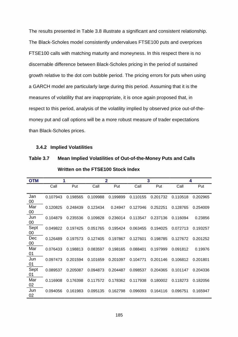
185

The results presented in Table 3.8 illustrate a significant and consistent relationship.

The Black-Scholes model consistently undervalues FTSE100 puts and overprices

FTSE100 calls with matching maturity and moneyness. In this respect there is no

discernable difference between Black-Scholes pricing in the period of sustained

growth relative to the dot com bubble period. The pricing errors for puts when using

a GARCH model are particularly large during this period. Assuming that it is the

measures of volatility that are inappropriate, it is once again proposed that, in

respect to this period, analysis of the volatility implied by observed price out-of-the-

money put and call options will be a more robust measure of trader expectations

than Black-Scholes prices.

3.4.2 Implied Volatilities

Table 3.7 Mean Implied Volatilities of Out-of-the-Money Puts and Calls

Written on the FTSE100 Stock Index

OTM 1 2 3 4

Call Put Call Put Call Put Call Put

Jan 00

0.107943 0.198565 0.109988 0.199899 0.110155 0.201732 0.110518 0.202965

Mar 00

0.120825 0.248439 0.123434 0.24947 0.127046 0.252251 0.128765 0.254009

Jun 00

0.104879 0.235536 0.109828 0.236014 0.113547 0.237136 0.116094 0.23856

Sept 00

0.049822 0.197425 0.051765 0.195424 0.063455 0.194025 0.072713 0.193257

Dec 00

0.126489 0.197573 0.127405 0.197867 0.127601 0.198785 0.127672 0.201252

Mar 01

0.076433 0.198813 0.083597 0.198165 0.088401 0.197999 0.091812 0.19976

Jun 01

0.097473 0.201594 0.101659 0.201097 0.104771 0.201146 0.106812 0.201801

Sept 01

0.089537 0.205087 0.094873 0.204487 0.098537 0.204365 0.101147 0.204336

Mar 02

0.116908 0.176398 0.117572 0.178362 0.117938 0.180002 0.118273 0.182056

Jun 02

0.094056 0.161983 0.095135 0.162798 0.096093 0.164116 0.096751 0.165947

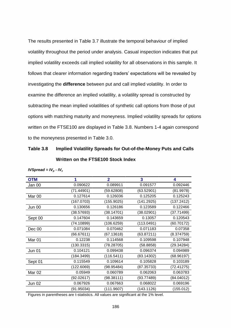
186

The results presented in Table 3.7 illustrate the temporal behaviour of implied

volatility throughout the period under analysis. Casual inspection indicates that put

implied volatility exceeds call implied volatility for all observations in this sample. It

follows that clearer information regarding traders‟ expectations will be revealed by

investigating the difference between put and call implied volatility. In order to

examine the difference an implied volatility, a volatility spread is constructed by

subtracting the mean implied volatilities of synthetic call options from those of put

options with matching maturity and moneyness. Implied volatility spreads for options

written on the FTSE100 are displayed in Table 3.8. Numbers 1-4 again correspond

to the moneyness presented in Table 3.0.

Table 3.8 Implied Volatility Spreads for Out-of-the-Money Puts and Calls

Written on the FTSE100 Stock Index

IVSpread = IVp - IVc

OTM 1 2 3 4

Jan 00 0.090622 0.089911 0.091577 0.092446

(71.44901) (59.62808) (63.52901) (81.9978)

Mar 00 0.127614 0.126036 0.125205 0.125243

(167.0703) (155.9025) (141.2925) (137.2412)

Jun 00 0.130656 0.126186 0.123589 0.122466

(38.57693) (38.14701) (38.02901) (37.71499)

Sept 00 0.147604 0.143659 0.13057 0.120543

(74.10899) (106.6259) (113.0491) (60.70172)

Dec 00 0.071084 0.070462 0.071183 0.07358

(66.67611) (67.13618) (63.87211) (8.374759)

Mar 01 0.12238 0.114568 0.109598 0.107948

(130.3315) (78.28705) (58.8858) (29.34284)

Jun 01 0.104121 0.099438 0.096374 0.094989

(184.3499) (116.5411) (83.14302) (68.96197)

Sept 01 0.115549 0.109614 0.105828 0.103189

(122.6069) (98.95484) (87.35733) (72.41275)

Mar 02 0.05949 0.060789 0.062063 0.063783

(92.02617) (98.38111) (93.77489) (84.04012)

Jun 02 0.067926 0.067663 0.068022 0.069196

(91.95034) (111.9607) (143.1126) (155.012)

Figures in parentheses are t-statistics. All values are significant at the 1% level.

187

All of the figures presented in Table 3.8 are significant and positive. This means that

the implied volatility of puts exceeds the implied volatility of calls throughout the

period. There is however evidence that the volatility smile evolves through time. The

implied volatility of puts relative to calls increases as we move from the January

2000 contract through the September 2000 contract. Following a narrowing of the

volatility spread for the December 2000 contract the implied volatility spread exceeds

10 percentage points until it narrows in 2002. Notably, moneyness seems to have

little impact on the magnitude of the spread during this period.

A sample of call and put implied volatility smirks are presented in Figure 3.4, Panels

A to F, to accompany the discussion of unorthodox preferences and the risk-neutral

distribution. The volatility smirks provide a graphic illustration of the behaviour of

implied volatility over time. It is clear that put implied volatility exceeds that of calls

with matching moneyness. There is also a pronounced skew with volatility increasing

as options are observed further out-of-the-money.

188

Table 3.9 Mean Implied Volatilities of Out-of-the-Money Puts and Calls Written

on the FTSE100 Stock Index Comparison Period

OTM 1 2 3 4

Call Put Call Put Call Put Call Put

Sept 98 0.079327 0.251099 0.074906 0.250355 0.084159 0.249994 0.090227 0.249804

Dec 98 0.126489 0.197573 0.127405 0.197867 0.127601 0.198785 0.127722 0.200129

Mar 99 0.209092 0.313832 0.208485 0.315207 0.207376 0.316696 0.205729 0.319163

Jun 99 0.112274 0.214564 0.114101 0.215656 0.115566 0.216464 0.116477 0.217312

Table 3.9 illustrates the temporal behaviour of implied volatility throughout the

comparative period. Perhaps the most notable feature of these results is the

increase in implied volatility used to price both put and call options maturing in March

1999 with a subsequent fall in each for the contract maturing in June 1999. On initial

inspection this pattern indicates that traders are concerned about the future volatility

of the market index and are hence using high estimates of implied volatility to price

options. However, at this stage it is not possible to infer the direction of expected

price changes that dominates.

Again, more information may be revealed by investigating the volatility spread

calculated from mean implied volatilities obtained from symmetrically distributed put

and synthetic call option prices. These are displayed in Table 3.10. Numbers 1-4

denote the moneyness as defined in Table 3.0 for the nearest to fourth-nearest out-

of-the-money contracts respectively.

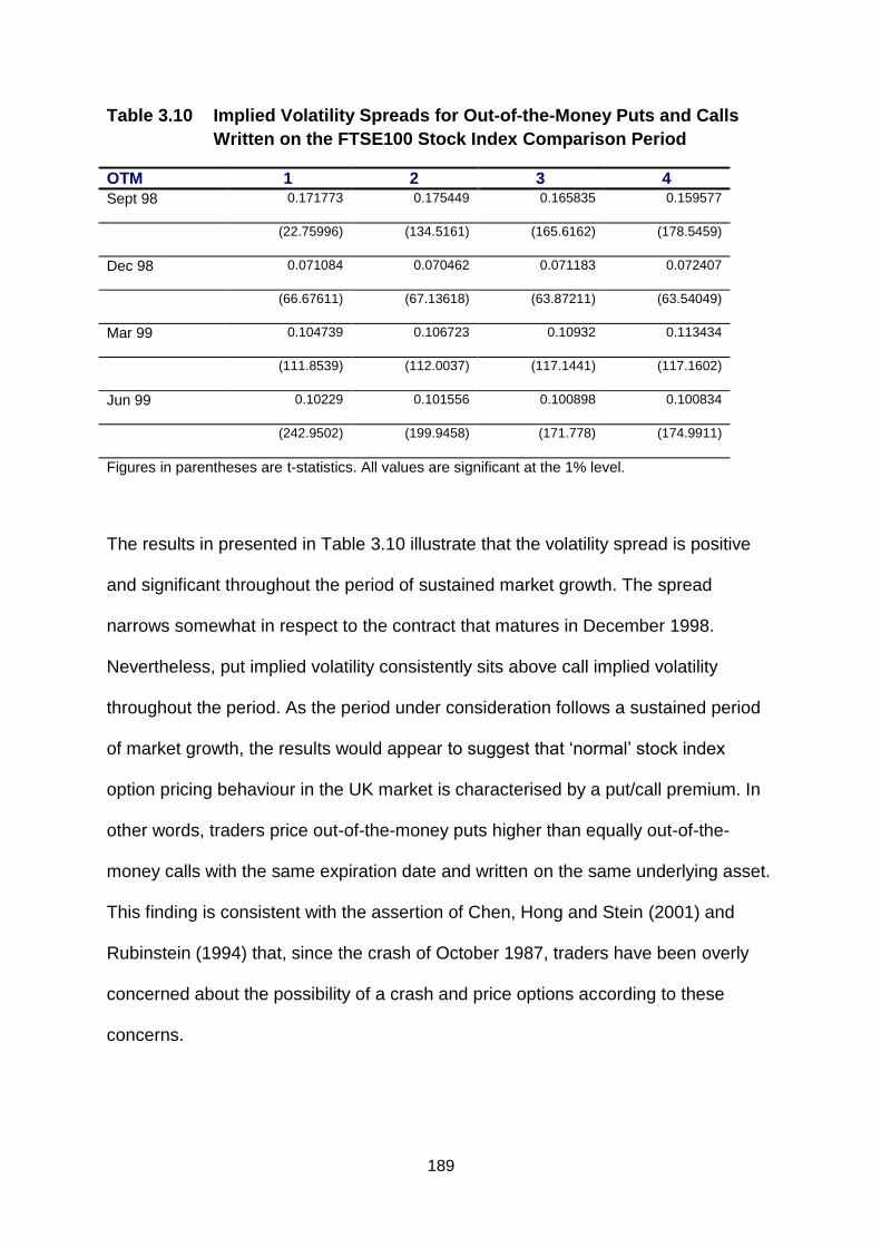
189

Table 3.10 Implied Volatility Spreads for Out-of-the-Money Puts and Calls

Written on the FTSE100 Stock Index Comparison Period

OTM 1 2 3 4

Sept 98 0.171773 0.175449 0.165835 0.159577

(22.75996) (134.5161) (165.6162) (178.5459)

Dec 98 0.071084 0.070462 0.071183 0.072407

(66.67611) (67.13618) (63.87211) (63.54049)

Mar 99 0.104739 0.106723 0.10932 0.113434

(111.8539) (112.0037) (117.1441) (117.1602)

Jun 99 0.10229 0.101556 0.100898 0.100834

(242.9502) (199.9458) (171.778) (174.9911)

Figures in parentheses are t-statistics. All values are significant at the 1% level.

The results in presented in Table 3.10 illustrate that the volatility spread is positive

and significant throughout the period of sustained market growth. The spread

narrows somewhat in respect to the contract that matures in December 1998.

Nevertheless, put implied volatility consistently sits above call implied volatility

throughout the period. As the period under consideration follows a sustained period

of market growth, the results would appear to suggest that „normal‟ stock index

option pricing behaviour in the UK market is characterised by a put/call premium. In

other words, traders price out-of-the-money puts higher than equally out-of-the-

money calls with the same expiration date and written on the same underlying asset.

This finding is consistent with the assertion of Chen, Hong and Stein (2001) and

Rubinstein (1994) that, since the crash of October 1987, traders have been overly

concerned about the possibility of a crash and price options according to these

concerns.

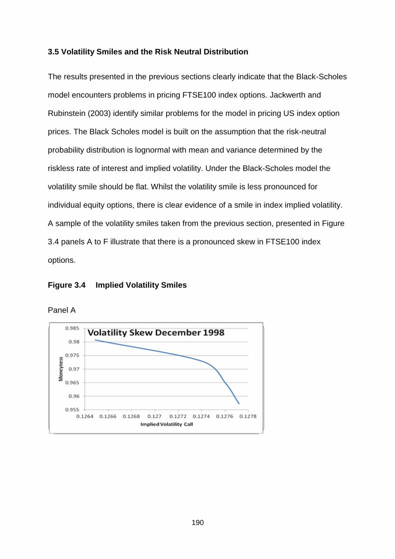
190

3.5 Volatility Smiles and the Risk Neutral Distribution

The results presented in the previous sections clearly indicate that the Black-Scholes

model encounters problems in pricing FTSE100 index options. Jackwerth and

Rubinstein (2003) identify similar problems for the model in pricing US index option

prices. The Black Scholes model is built on the assumption that the risk-neutral

probability distribution is lognormal with mean and variance determined by the

riskless rate of interest and implied volatility. Under the Black-Scholes model the

volatility smile should be flat. Whilst the volatility smile is less pronounced for

individual equity options, there is clear evidence of a smile in index implied volatility.

A sample of the volatility smiles taken from the previous section, presented in Figure

3.4 panels A to F illustrate that there is a pronounced skew in FTSE100 index

options.

Figure 3.4 Implied Volatility Smiles

Panel A

Mo

ne

yne

ss

Implied Volatility Call

Volatility Skew December 1998

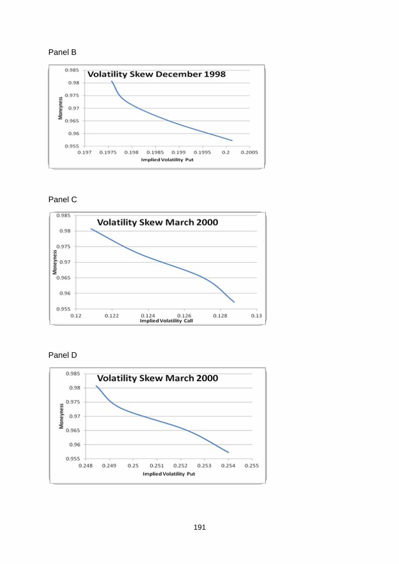
191

Panel B

Panel C

Panel D

Mo

ne

yne

ss

Implied Volatility Put

Volatility Skew December 1998 M

on

eyn

ess


Volatility Skew March 2000

Mo

ne

yne

ss


Volatility Skew March 2000

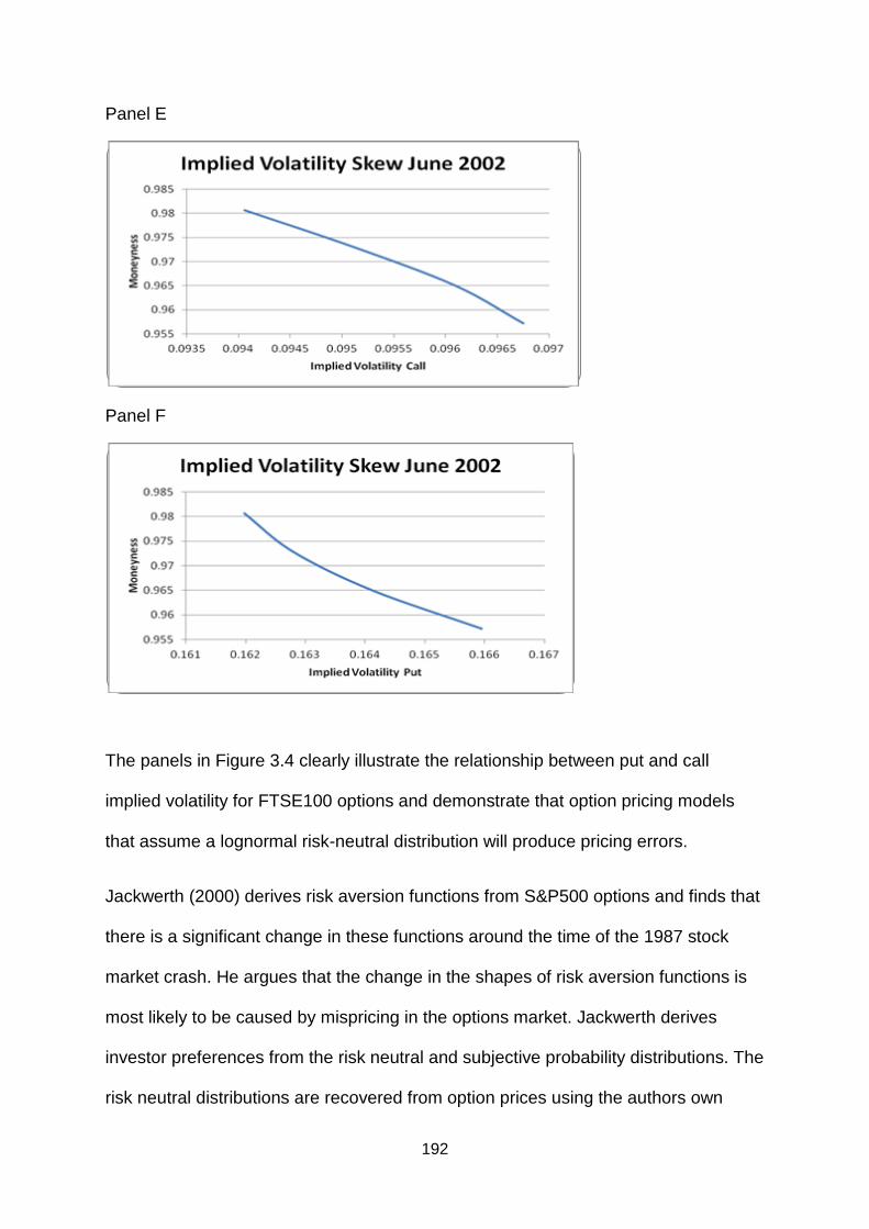
192

Panel E

Panel F

The panels in Figure 3.4 clearly illustrate the relationship between put and call

implied volatility for FTSE100 options and demonstrate that option pricing models

that assume a lognormal risk-neutral distribution will produce pricing errors.

Jackwerth (2000) derives risk aversion functions from S&P500 options and finds that

there is a significant change in these functions around the time of the 1987 stock

market crash. He argues that the change in the shapes of risk aversion functions is

most likely to be caused by mispricing in the options market. Jackwerth derives

investor preferences from the risk neutral and subjective probability distributions. The

risk neutral distributions are recovered from option prices using the authors own

Mo

ne

yne

ss


Implied Volatility Skew June 2002

Mo

ne

yne

ss


Implied Volatility Skew June 2002

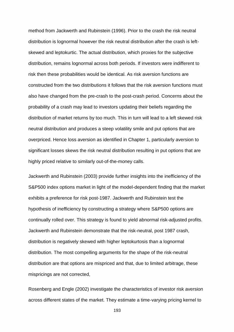
193

method from Jackwerth and Rubinstein (1996). Prior to the crash the risk neutral

distribution is lognormal however the risk neutral distribution after the crash is left-

skewed and leptokurtic. The actual distribution, which proxies for the subjective

distribution, remains lognormal across both periods. If investors were indifferent to

risk then these probabilities would be identical. As risk aversion functions are

constructed from the two distributions it follows that the risk aversion functions must

also have changed from the pre-crash to the post-crash period. Concerns about the

probability of a crash may lead to investors updating their beliefs regarding the

distribution of market returns by too much. This in turn will lead to a left skewed risk

neutral distribution and produces a steep volatility smile and put options that are

overpriced. Hence loss aversion as identified in Chapter 1, particularly aversion to

significant losses skews the risk neutral distribution resulting in put options that are

highly priced relative to similarly out-of-the-money calls.

Jackwerth and Rubinstein (2003) provide further insights into the inefficiency of the

S&P500 index options market in light of the model-dependent finding that the market

exhibits a preference for risk post-1987. Jackwerth and Rubinstein test the

hypothesis of inefficiency by constructing a strategy where S&P500 options are

continually rolled over. This strategy is found to yield abnormal risk-adjusted profits.

Jackwerth and Rubinstein demonstrate that the risk-neutral, post 1987 crash,

distribution is negatively skewed with higher leptokurtosis than a lognormal

distribution. The most compelling arguments for the shape of the risk-neutral

distribution are that options are mispriced and that, due to limited arbitrage, these

mispricings are not corrected,

Rosenberg and Engle (2002) investigate the characteristics of investor risk aversion

across different states of the market. They estimate a time-varying pricing kernel to

194

produce a risk-neutral distribution that is less leptokurtic and less left-skewed than

that of Jackwerth (2000). They estimate their empirical pricing kernel using S&P500

index prices and option payoff probabilities. The empirical pricing kernel is then the

preference function that best fits actual prices. Rosenberg and Engle‟s results

demonstrate that investors become more risk averse during recessions and less risk

averse during periods of growth. This is demonstrated by examining the correlation

between empirical risk aversion and the width of the credit spread and also with the

steepness of the term structure slope. They find negative correlation with the former

and positive with the latter.

Bondarenko (2003) attempts to explain what he terms the „overpriced puts puzzle‟ in

an equilibrium framework as opposed to the partial equilibrium frameworks of Hull

and White (1987) and Heston (1993). To contextualise the extent of put

expensiveness he notes that for S&P500 at-the-money puts to break even, crashes

of the magnitude of the 1987 crash would need to occur 1.3 times per year. More

importantly the trade in puts accounts for a significant transfer of wealth from buyers

to sellers. Bondarenko argues that Jackwerth‟s kernel pricing puzzle may be

spurious as it is wrongly based on the assumption that the pricing kernel is a function

of the value of the market portfolio. He also finds that standard equilibrium models

(CAPM and Rubinstein (1976)) are incompatible with the level of put prices.

Bondarenko uses a model-free equilibrium approach where the fair compensation for

taking the risk involved in writing puts depends on a non-standard equilibrium model

of risk and return and incorporates a rationality restriction. The risk neutral

distribution is estimated non-parametrically from S&P500 option prices. However, the

model is unable to explain the high price of put options.

195

The literature which uses unorthodox preferences, such as loss aversion and time-

varying risk-aversion, to explain the shape of the risk-neutral distribution goes some

way towards explaining the shape and the evolution of the volatility smile for index

options.

3.5 Conclusion

The analysis of FTSE100 put and call option prices matched by moneyness and

maturity fails to provide any conclusive evidence of return predictability for the

FTSE100 index. Puts are priced more highly than calls during the dot com bubble

boom and burst around the turn of the century. However, the relationship is found to

be comparable during a period of sustained growth. Over the entire period it is

apparent that there is no consistent way in which market moves can be predicted

using stock index option prices hence market efficiency cannot be rejected on these

grounds.

The Black-Scholes model, which assumes a lognormal risk-neutral distribution,

significantly undervalues puts and overvalues calls across the period under

investigation. The only exceptions occur in a short period across the final quarter of

2001. The finding of under- and overvaluation is robust across four different

moneyness categories and to the use of static and time-varying volatility estimates.

This finding motivates an analysis of implied volatility and implied volatility spreads.

The volatility spreads indicate that implied volatility of FTSE100 puts lies consistently

above that of corresponding calls. The implied volatility itself indicates a pronounced

volatility skew which is clear from the charts in section. 3.5. The evolution of the

smile does not imply predictability but it does appear that options market investors

react to events in the market. For example the highest put implied volatility is

observed for the contract which matures in March 2000. The option prices used in

196

backing out this implied volatility were observed in January and February of 2000,

immediately after the bubble burst.

The apparent mispricing of FTSE100 options indicates that there are implicit crash

fears in the UK market and these pre-date the dot com bubble. The shape of the

volatility smiles indicate that option investors are loss-averse and particularly averse

to the extreme losses that can be suffered as a result of a crash. When implicit crash

fears are priced, option prices reveal a risk-normal distribution which is not

lognormal. Hence it is unsurprising that there are significant pricing errors when a

Black-Scholes model is used to price FTSE100 index options.

Generally, it seems that traders‟ fear of downside risk dominates their perception of

upside potential. Put simply, traders are aware that market crashes occur and, when

they do, losses are likely to be substantial. Thus, the put option premium is

analogous to an insurance policy against a significant event that has been witnessed

in recent history. Overall, the results presented in this chapter provide motivation of a

more in-depth analysis of implied volatility in UK markets.

197

Chapter 4

Was the 2007 Crisis Expected?

An Analysis of Implied Volatility in UK

Index Options Markets

198

4.1 Introduction and Motivation

The first major financial crisis of the 21st century began in mid-2007 when the losses

associated with subprime lending became apparent. This was quickly followed by

events such as the closure of Dillon Reed, bailout of Bear Stearns‟ hedge funds,

bankruptcy of American Home Mortgages, plight of Northern Rock, bailout of AIG

and collapse of Lehman Brothers.20 In an efficient capital market the assumption

would be that the financial crisis and credit crunch could not have been predicted; it

was new information that would be impounded into prices as soon as it became

publicly available. However it is clear that the seeds of the crisis were sown in the

years prior to 2007 which raises the question as to whether professional option

traders may have anticipated the crisis.

As discussed in Chapter 3, if option traders were privy to information prior to an

extreme market event, or period of turbulence regarding the probability of such an

event occurring, then clearly this would be priced into option premiums. More

precisely, the demand for stock index put options would exceed that for stock index

calls with a similar degree of moneyness. Option writers would react to the higher

demand and perceived information signal and adjust the prices of index options

accordingly. If investors are able to anticipate financial crises then this will allow

them to re-balance their portfolios and hence insulate them from the most damaging

impacts. The availability of volatility indexes and their interpretation as a gauge of

investor sentiment provides an additional means by which to analyse market

predictability.

An alternative approach to that employed in Chapter 3 is taken in Chapter 4 where

the focus will be on implied volatility indexes such as the VIX and VFTSE. Index

20

Pilbeam (2010) provides a detailed timeline of key events in the financial crisis.

199

option implied volatility incorporates investor expectations and, if investor

expectations turn out to be correct on average, it should provide a useful predictor of

future spot market behaviour. Furthermore, implied volatility is a widely recognised

and important gauge of expected future volatility as investors are considering options

which mature over a range of future exercise dates. This chapter provides an

important contribution to the literature as a unique volatility index is constructed to

facilitate examination of the relationship between implied volatility and the UK stock

market prior to the introduction of the VFTSE in 2008.

This key objective of this chapter will be to examine and seek to address a number

of important questions:

Do the contemporaneous relationships between volatility indexes and UK

stock market returns support the notion of „fear indexes‟?

Do volatility indexes contain any predictive power for the actual, or realised,

volatility of stock indexes?

Do volatility indexes contain any predictive power for aggregate stock market

returns?

To what extent can volatility indexes provide an insight into investor sentiment

before, during and after the recent financial crisis?

200

4.2 Literature Review

The VIX is the Chicago Board Options Exchange (CBOE) volatility index which

calculates the implied volatility of American-style S&P 500 options over a 30-day

horizon. It is a weighted average of the implied volatilities of eight call and put

options which are close-to-the-money. The VIX serves as an indicator of optimism

and pessimism and hence is sometimes referred to, for example by Whaley (2000),

as the „fear indicator‟. Simon (2003) adds that the level of the VIX indicates the price

investors are willing to pay in terms of implied volatility to hedge stock portfolios with

index put options or to take long positions in index calls. Moreover Simlai (2010)

expands the notion of the VIX as a fear index to a barometer of investor sentiment in

both bullish and bearish markets. It can be interpreted as market participants‟

consensus view of expected future stock market volatility.

A number of studies have used implied volatility as a means to predict future

volatility. Prominent articles are those by Day and Lewis (1992), Lamoureux and

Lastrapes (1993), Fleming (1998) and Christensen and Prabhala (1998).

Day and Lewis (1992) compare the volatility forecasting performance of Black-

Scholes-Merton implied volatility extracted from S&P 100 stock index options with

forecasts produced using GARCH models on weekly data. They find that implied

volatility may offer incremental information relative to conditional volatility provided

by GARCH and EGARCH models and vice versa. This indicates that neither method

completely characterises in-sample stock market volatility.

Lamoureux and Lastrapes (1993) investigate the implied volatility of at-the-money

call options using the Hull and White (1987) stochastic volatility model and compare

its forecasting performance with that of a GARCH model. Lamoureux and Lastrapes

201

extend the work of Day and Lewis by investigating daily data on individual stock

options traded on the CBOE between 1982 and 1984 and by testing an out-of-

sample model. Lamoureux and Lastrapes reject the option pricing model as a price-

determining market mechanism but do find that the model can be adjusted to provide

important information for forecasting stock variance over a 90 to 180 day horizon.

Canina and Figlewski (1993) investigate the informational content of implied volatility

extracted from American-style S&P 100 options. Closing prices for the sample period

March 1983 to March 1987 are input into a binomial option pricing model. The

implied volatilities produced exhibit a clear volatility skew. Canina and Figlewski‟s

key finding is that implied volatility is not a good estimate of the market expectation

of realised volatility. Furthermore implied volatility is incorporated into past volatility

which, in turn, is significantly related to future volatility. However the bulk of the

subsequent literature contradicts these findings. Christensen and Prabhala (1998)

use monthly observations over a longer time period to produce evidence in contrast

to that of Canina and Figlewski. Christensen and Prabhala also investigate S&P 100

implied volatility but use non-overlapping data for the period November 1983 to May

1995. The authors find that, despite producing biased forecasts, implied volatility

does predict realised future volatility and incorporates historical volatility.

Furthermore, the predictive power of implied volatility is found to improve following

the 1987 stock market crash. Jorion (1995) produces evidence from currency options

that contrasts with that of Canina and Figlewski. He finds that implied volatility

estimates outperform GARCH models in forecasting future volatility.

Fleming (1998) also considers the implied volatility of S&P 100 options and

compares this to historical volatility and conditional volatility produced by GARCH

models. Fleming finds that implied volatility produces biased forecasts although it is

202

unclear whether this is a result of option market inefficiency or misspecification of the

volatility process in the option pricing model. He also finds that implied volatility

produces useful estimates of future volatility which are independent of those

produced by a GARCH model. Fleming concludes by highlighting the importance of

implied volatility as a measure of investor sentiment, a potential input for asset

pricing and an indicator of expected returns.

Fleming, Ostdiek and Whaley (1995) examine the predictive power of the VIX for

future realised stock market volatility. They perform their analysis on daily and

weekly returns on the S&P 100 index and changes in the VIX over the period 1986 to

1992. Fleming et al find evidence of significant negative contemporaneous

correlation between changes in the VIX and returns on the S&P 100. Hence high

volatility is associated with negative stock market moves and vice versa. Interestingly

the effect is asymmetric with larger absolute changes in volatility associated with

negative returns as opposed to positive returns of equivalent magnitude. Fleming et

al also find the VIX to be a good predictor of realised future stock market volatility

and add that it imbeds the expectations of market participants.

Blair, Poon and Taylor (2001) compare the predictive ability of implied volatility with

that of ARCH models using daily data on the VIX and S&P 100. They also use high

frequency intraday data on the index to compute a measure of realised volatility. The

sample period is from January 1987 to December 1999. The authors also consider

how important the choice of measure of realised volatility is to the predictive power of

volatility forecasts. Blair, Poon and Taylor find that in-sample ARCH models provide

no additional information on index returns over and above that provided by the VIX.

Moreover little further information is produced by the inclusion of the high frequency

203

returns. For out-of-sample forecasts the VIX outperforms all other methods tested in

terms of accuracy.

Martens and Zein (2004) consider volatility forecasts using publicly available high

frequency data. The S&P 500 index and associated option contract is examined

along with currency futures and options on the YEN/USD and on crude oil. Martens

and Zein‟s findings indicate that implied volatility outperforms a GARCH(1,1) model

in each case for daily data. For high frequency data the GARCH extended with high

volatility forecasts outperforms the GARCH extended with realised volatility.

However, when realised volatilities are produced using squared high frequency

returns, long memory GARCH forecasts can at least match the performance, and in

some cases outperform the implied volatility forecasts. Martens and Zein note that

each type of forecast contains information which is not contained in the other.

A further comparative analysis based on the S&P 100 and the VIX is conducted by

Koopman, Jungbacker and Hol (2005) who employ intraday data. Koopman et al

investigate a variety of models to produce a ranking of volatility forecasts. They

conclude that the most accurate forecasts of realised volatility can be produced

using an autoregressive fractionally integrated moving average model followed by

those produced using an unobserved components model.

Giot (2005) examines both the contemporaneous relationship between implied

volatility and returns and the relationship between implied volatility and future returns

using daily return data from August 1994 to January 2003. The sample period

includes bull and bear markets and periods of high and low volatility. Giot

demonstrates that there is a negative and significant relationship between the

contemporaneous returns on the S&P 500 index and the VIX and VXN volatility

204

indexes21. Giot also found weak evidence of a positive relationship between future

returns and implied volatility indexes. Similar relationships were found by Simlai

(2010) although the results presented also indicate that there is a strong information

flow from the S&P 500 to the VIX. Simlai examines correlations in index option

implied volatility using the VIX, the 10-year US T-bill rate and the S&P 500. The

period under investigation covers the technology boom from 1995 to 2001. Simlai

selects daily data and employs a variety of GARCH models to examine whether the

variability of index option implied volatility is driven by market information. The key

findings are the aforementioned significant flow of information from the S&P 500 to

the VIX and that high implied volatility is associated with falling index values.

Simon (2003) investigates the relationship between the NASDAQ 100 index (NDX)

and its associated VXN volatility index. He finds that the response of the VXN to

changes in the NASDAQ 100 index is remarkably stable for the duration of the

technology stock bubble of the late 1990s/2000 and beyond. In particular the

volatility index falls in response to large positive returns on the underlying index and

rises in response to large negative returns. However he also finds that, although the

VXN has predictive power for actual volatility, it consistently predicts higher volatility

than is realised. Furthermore, he finds that over the entire sample period greater

positive and negative deviations of the NDX from its 5-day moving average lead to

statistically significant greater increases in the VXN. Simon offers reconciliation of

this finding with the finding that positive NDX returns are associated with greater

VXN declines. He explains that positive returns per se reduce fear and hence lead to

reduced demand for puts for hedging and for calls in their role as a low risk position

in a stock. However sustained upward deviations from a moving average are

21

The VXN is an index that is constructed from implied volatility of close-to-the-money, near maturity

American-style option contracts on the NASDAQ100 index.

205

perceived as a trend in the NDX. This in turn makes long calls more attractive due to

the convexity of delta. Interestingly, during the bubble period negative deviations of

the NDX from its 5-day moving average were not associated with higher increases in

the VXN. Simon offers a plausible explanation that deviations were not perceived as

signalling a downward trend because the overall trend had been overwhelmingly

positive. The relationship in the post-bubble period is found to be consistent with that

for the entire sample period.

Simon considers why the VXN moves in opposite directions in response to large

positive and negative NDX returns and summarises with three key explanations:

1. Implied volatility reflects how actual volatility reacts to positive and negative

returns.

2. The VXN is driven by option trading dynamics. The insurance demand for

puts and demand for calls as a low-risk equity position rise in response to

negative returns on the underlying. During market rallies market participants

are inclined to purchase less puts for hedging purposes and are more willing

to hold equities as the perception of downside risk is less salient.

3. The commonly observed volatility skew reflects higher implied volatilities for

options with low exercise prices. As equity prices rise, at-the-money options

have higher exercise prices and lower implied volatilities than those previously

at-the-money. As at-the-money options are used to compute volatility indexes,

the volatility skew may partly explain the tendency of market rallies to be

associated with falling implied volatility and declines with rising implied

volatility.

206

The vast majority of studies of the forecasting power of implied volatility have

examined index options whilst there are apparently very few studies published that

investigate the information content of implied volatility of single stock options.

Notable exceptions are those published by Gemmill and Dickins (1986), Lamoureux

and Lastrapes (1993) and Taylor, Yadav and Zhang (2010).

Gemmill and Dickens (1986) examine the prices of equity call options of 16

companies listed on the London traded options market. Their objective is to examine

whether the Black Scholes model can be used to identify mispriced options and

whether profitable strategies can be constructed as a result. Delta hedged portfolios

are constructed which yield significant positive returns, however the positive returns

do not survive the inclusion of transactions costs. Hence the market efficiency

cannot be rejected for the period under analysis (1978-1983) and inferences are

difficult to draw due to non-synchronous trading of stocks and options.

Lamoureux and Lastrapes (1993) employ the Hull and White (1987) model to test the

orthogonality restriction that information available when market prices are set is not

superior to implied variance in predicting realised return variance using CBOE

options and associated stocks. Implied variances are collected from at-the-money

call options written on individual stocks whilst a GARCH model is used to predict

return variance from market prices. The key findings are that implied variance

significantly underpredicts realised variance and that forecasts from past returns

contain relevant information additional to that contained in implied variance.

Taylor, Yadav and Zhang (2010) adopt a model-free approach to investigate the

information content of implied volatility for 149 US firms for the period January 1996

to December 1999. The advantage of selecting a model-free approach is that such

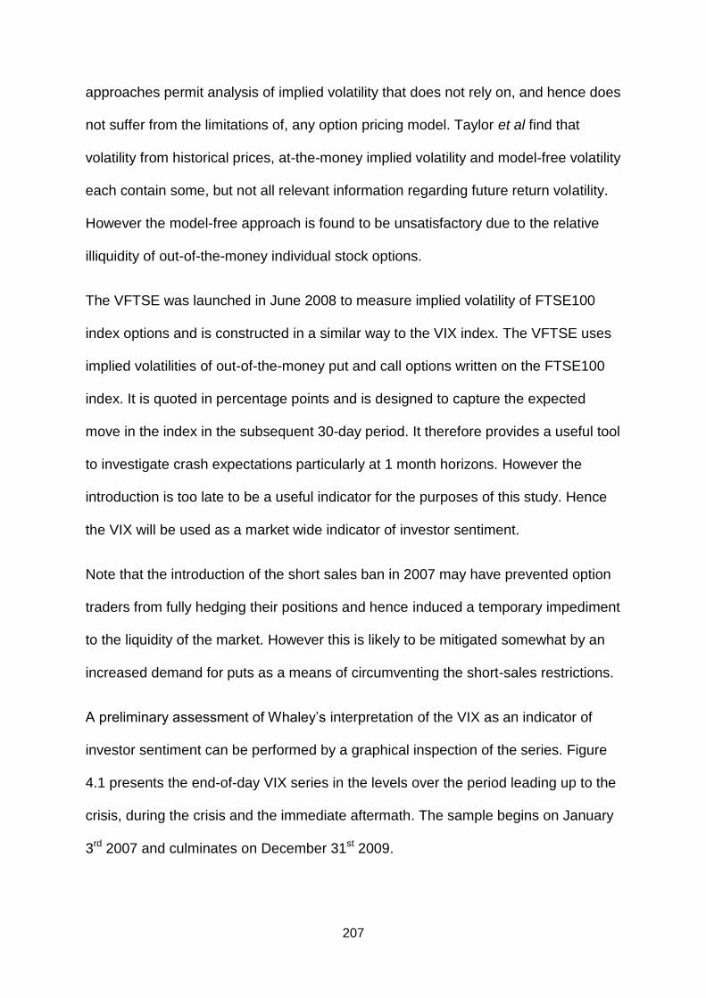
207

approaches permit analysis of implied volatility that does not rely on, and hence does

not suffer from the limitations of, any option pricing model. Taylor et al find that

volatility from historical prices, at-the-money implied volatility and model-free volatility

each contain some, but not all relevant information regarding future return volatility.

However the model-free approach is found to be unsatisfactory due to the relative

illiquidity of out-of-the-money individual stock options.

The VFTSE was launched in June 2008 to measure implied volatility of FTSE100

index options and is constructed in a similar way to the VIX index. The VFTSE uses

implied volatilities of out-of-the-money put and call options written on the FTSE100

index. It is quoted in percentage points and is designed to capture the expected

move in the index in the subsequent 30-day period. It therefore provides a useful tool

to investigate crash expectations particularly at 1 month horizons. However the

introduction is too late to be a useful indicator for the purposes of this study. Hence

the VIX will be used as a market wide indicator of investor sentiment.

Note that the introduction of the short sales ban in 2007 may have prevented option

traders from fully hedging their positions and hence induced a temporary impediment

to the liquidity of the market. However this is likely to be mitigated somewhat by an

increased demand for puts as a means of circumventing the short-sales restrictions.

A preliminary assessment of Whaley‟s interpretation of the VIX as an indicator of

investor sentiment can be performed by a graphical inspection of the series. Figure

4.1 presents the end-of-day VIX series in the levels over the period leading up to the

crisis, during the crisis and the immediate aftermath. The sample begins on January

3rd 2007 and culminates on December 31st 2009.

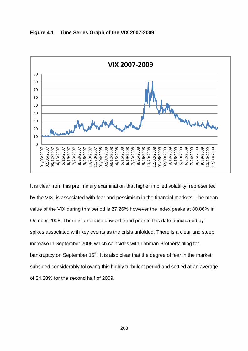
208

Figure 4.1 Time Series Graph of the VIX 2007-2009

It is clear from this preliminary examination that higher implied volatility, represented

by the VIX, is associated with fear and pessimism in the financial markets. The mean

value of the VIX during this period is 27.26% however the index peaks at 80.86% in

October 2008. There is a notable upward trend prior to this date punctuated by

spikes associated with key events as the crisis unfolded. There is a clear and steep

increase in September 2008 which coincides with Lehman Brothers‟ filing for

bankruptcy on September 15th. It is also clear that the degree of fear in the market

subsided considerably following this highly turbulent period and settled at an average

of 24.28% for the second half of 2009.

0

10

20

30

40

50

60

70

80

90

01

/03

/20

07

02

/06

/20

07

03

/12

/20

07

4/1

3/2

00

7

5/1

6/2

00

7

6/1

9/2

00

7

7/2

3/2

00

7

8/2

3/2

00

7

9/2

6/2

00

7

10

/29

/20

07

11

/30

/20

07

01

/04

/20

08

02

/07

/20

08

03

/12

/20

08

4/1

5/2

00

8

5/1

6/2

00

8

6/1

9/2

00

8

7/2

3/2

00

8

8/2

5/2

00

8

9/2

6/2

00

8

10

/29

/20

08

12

/02

/20

08

01

/06

/20

09

02

/09

/20

09

3/1

3/2

00

9

4/1

6/2

00

9

5/1

9/2

00

9

6/2

2/2

00

9

7/2

4/2

00

9

8/2

6/2

00

9

9/2

9/2

00

9

10

/30

/20

09

12

/03

/20

09

VIX 2007-2009

209

4.3 Initial Tests to Examine the VIX/VFTSE Relationship

4.3.1 Introduction

In order to establish whether the VIX is an appropriate proxy for the VFTSE a

number of tests were run using daily opening, closing, high and low values, and,

more importantly, using the closing value of the VIX on the opening value of the

VFTSE. Gemmill and Kamayama (2000) demonstrate, using a vector autoregressive

model, that changes in the implied volatility of the UK market on a given day are

driven by lagged changes in implied volatility of the US market. This result accords

with intuition as the US market closes 6 hours (Central Time in Chicago) after the

close of markets in London. It follows that the strongest relationship should be

between the opening value of the VFTSE on day n and the closing value of the VIX

on day n-1. Gemmill and Kamayama also examine for similar spillover effects using

the Nikkei 225.

This range of values examined should mitigate against the non-contemporaneous

nature of opening and closing values arising from the time difference between the

UK and US.

4.3.2 Data

Historical daily price data for opening, closing, high and low values for the VIX are

collected from the Chicago Board Options Exchange (CBOE). Corresponding values

for the VFTSE are collected from Euronext LIFFE. It is necessary to select a fairly

recent sample period given the limited VFTSE data availability. Hence the data

selected cover the period from 4/1/2010 until 29/3/2011. Figure 4.2 provides a visual

inspection of the relationship between closing values of the two series:

210

Figure 4.2 Time Series Graph of the VIX and VFTSE 2010-2011 (Closing)

The shape of each index series is very similar although for most periods implied

volatility is higher in the US than in the UK particularly in the major spikes between

April and June 2010. It appears that in some periods the VIX leads the VFTSE whilst

in others the relationship is reversed. Overall it appears that the VIX moves prior to

the VFTSE strengthening the case for examining the relationship between the

closing values of the VIX and the opening values of the VFTSE.

The initial test performed was a simple correlation to determine the relationship

between the series:

∑( )( )

√∑( ) ∑( ) (4.1)

Running equation 4.1 produced the following coefficients where subscripts indicate

opening, closing, high, low and close on open values respectively.

Table 4.1: Correlation Between VIX and VFTSE

ρo ρc ρh ρl Ρco

Coefficient 0.610864 0.721895 0.750183 0.647782 0.6267

0

5

10

15

20

25

30

35

40

45

50

04

/01

/20

10

04

/02

/20

10

04

/03

/20

10

04

/04

/20

10

04

/05

/20

10

04

/06

/20

10

04

/07

/20

10

04

/08

/20

10

04

/09

/20

10

04

/10

/20

10

04

/11

/20

10

04

/12

/20

10

04

/01

/20

11

04

/02

/20

11

04

/03

/20

11

VIXC

VFTSEC

211

The results in table 4.1 provide support for the graphical representation in Figure 4.2.

The fairly strong positive correlation indicates that the two volatility series move

together over time although does not indicate the direction of causation.

4.3.3 OLS Regression Analysis and Unit Root Tests

To further examine the relationship the following OLS regression was also run, again

using daily opening, closing, high and low values:

(4.2a)

In addition, the following OLS regression was run for VIX closing on VFTSE

opening:

(4.2b)

Table 4.2: OLS Regression Results for Equation 4.2

Coefficient Standard Error

t- statistic (p) R2

Opening 0.506943 0.037696 13.47453 (8.67E-33) 0.373154

Closing 0.494773 0.027158 18.21865 (1.08E-50) 0.521132

High 0.511366 0.025809 19.81366 (9.79E-57) 0.5627755

Low 0.469756 0.031634 14.84989 (6.49E-38) 0.419622

Closing on Opening

0.522492 0.037262 14.02211(0.0000) 0.392752

The results presented in Table 4.2 indicate a positive and significant relationship

between the two series. However care must be taken to examine for a unit root in

each series in order to guard against spurious interpretation of the regression

results. Hence it was proposed that the following augmented Dickey-Fuller test, with

a null hypothesis of a unit root, was performed on each series:

∑ (4.3)

212

Where yt relates to each individual series for the VIX and VFTSE. The test is initially

performed without a time trend as we would not expect to find a deterministic trend in

a volatility index. However for completeness the test was subsequently run with the

inclusion of a time trend.

The running of a Breusch-Godfrey LM test confirmed the presence of serial

correlation in the VIX and in the VFTSE. An Augmented Dickey-Fuller test with a

maximum of 2 lags of the dependent variable was found to be appropriate. 3 lags of

the dependent variable were required to remove the serial correlation in VFTSE

opening values when a deterministic trend is included. The results are presented in

Tables 4.3(a) and 4.3(b). Subscripts o, c, h and l are used to denote opening closing,

high and low values respectively.

Table 4.3 (a) Augmented Dickey-Fuller Test Results (Constant)

DF t-Statistic Prob Unit Root Lags DF t-statistic 1st Diff

VIXo -3.117215* 0.0263 Y 2 -18.45321

VIXc -3.358579** 0.0132 Y 2 -18.24469

VIXh -3.189547** 0.0216 Y 2 -16.40145

VIXl -2.915457* 0.0447 Y 2 -17.82849

VFTSEo -3.555261 0.0073 N 1 -15.53693

VFTSEc -3.173655* 0.0225 Y 1 -16.80101

VFTSEh -3.170122* 0.0228 Y 1 -17.23061

VFTSEl -4.137819 0.0010 N 2 -23.27591 ***significant at the 1% level, ** significant at the 5% level, * significant at the 10% level

Table 4.3 (b) Augmented Dickey-Fuller Test Results (Constant & trend)

DF t-Statistic Prob Unit Root Lags DF t-statistic 1st Diff

VIXo -3.248282* 0.0771 Y 2 -18.42716

VIXc -3.521989** 0.0388 Y 2 -18.22055

VIXh -3.344442* 0.0612 Y 2 -16.37877

VIXl -3.067644*** 0.1160 Y 2 -17.80482

VFTSEo -3.854432* 0.0151 Y 3 -15.51366

VFTSEc -3.361460** 0.0586 Y 1 -16.77698

VFTSEh -3.333089** 0.0629 Y 1 -17.20848

VFTSEl -4.304823 0.0035 N 1 -23.23913 ***significant at the 1% level, ** significant at the 5% level, * significant at the 10% level

213

In the levels, for the majority of cases, the test statistic does not exceed the critical

value at least at the 10% level. Therefore the null hypothesis of a unit root in the

volatility series cannot be rejected. All series are found to be difference stationary.

Hence all series except for VFTSEO and VFTSEL are integrated of order 1 or I(1).

The results are largely insensitive to the inclusion of the trend term other than

VFTSEO which is found to contain a unit root when the trend is included.

4.3.4 Granger Causality Tests

Granger (1969) pioneered the analysis of causality in financial data. In order to

establish the likelihood of any temporal directional effects Granger Causality tests

are performed. This involves testing whether past values of variable „x‟ are able to

significantly explain current values of variable „y‟ once past values of „y‟ have been

controlled for. If this is found to be the case then „x‟ can be said to Granger cause „y‟.

The same test can then be repeated to establish whether „y‟ Granger Causes „x‟. The

first-differenced or returns series must be used because an assumption in Granger

Causality is that the series under consideration are stationary. Granger Causality is

also based on the fundamental assumption that the past can predict the future but

the future cannot predict the past. Tests of causality in the context of this study are

used to further establish the relationship between the VIX and VFTSE and hence

add weight to the justification for using the former as a proxy for the latter.

Table 4.4 contains the results of Granger Causality tests using four lags, with optimal

lag length selected using the akaike information criterion. The F-statistics are

reported for each direction. Figures in parentheses are probability values.

214

Table 4.4: Granger Causality Tests of the Relationship between the VIX and

the VFTSE Volatility Indexes

US indicates the first difference of the VIX and UK indicates the first difference of the

VFTSE.

Direction US → UK UK → US

Opening 3.88710 (0.00430)*** 2.73896 (0.02900)**

Closing 8.92138 (8.2E-07)*** 3.04702 (0.01749)**

High 18.8761 (8.0E-14)*** 4.85753 (0.00083)***

Low 8.19787 (2.8E-06)*** 1.78305 (0.13220)

Closing on Opening

5.74277 (0.0002)*** 2.84356 (0.0244)

***significant at the 1% level, **significant at the 5% level. Figures in parentheses are p-values.

The preliminary results in table 4.4 indicate that there are relationships between the

VIX and the VFTSE. For all pairs of variables UK implied volatility appears to react

significantly to US implied volatility. Furthermore, for the opening and closing pairs,

US implied volatility appears to react significantly to UK implied volatility. Most

importantly, opening UK implied volatility reacts significantly to closing US implied

volatility. These results should be interpreted with caution however because they are

sensitive to the choice of lag length. In addition, a finding that „x‟ does not Granger

Cause „y‟ does not necessarily imply that „x‟ and „y‟ are independent.

215

4.3.5 Cointegration Tests

Given that pairs of closing and high values including a constant and pairs of opening,

closing and high values including a constant and trend are non-stationary in the

levels but stationary in first-differences, it would seem reasonable to proceed with

cointegration tests on these variables. Results are presented for all pairs for

completeness. Where two series are integrated of order one [I(1)], it may be possible

to combine these series to produce a series with a lower order of integration. In other

words, this method is used to establish if the series are cointegrated. The finding of

cointegration indicates a stable long-run equilibrium relationship between the two

series.

The Engle and Granger (1987) procedure is employed which first involves running

the following cointegrating regressions for the respective pairs of series:

(4.4a)

(4.4b)

The regression is underpinned by an assumption that the direction of causation is

from the US to the UK. This seems to be a reasonable assumption given the

strength of the Granger Causality results. The residuals produced from the

regression will correspond to the error in equilibrium. These residuals are then tested

for a unit root using an ADF test. If it is inferred that the residuals do not contain a

unit root and hence the error term is stationary, then the null hypothesis that the two

difference series are not cointegrated will be rejected. This then permits inference

that there is a meaningful relationship between the series.

216

Table 4.5 Results of Engle Granger Cointegration Tests

Constant Constant & Trend

-statistic Probability -statistic Probability

Opening -5.600462 0.0000 -5.816573 0.0000

Closing -5.5992663 0.0000 -6.10042 0.0000

High -6.074444 0.0000 -6.129917 0.0000

Low -6.370623 0.0000 -6.436467 0.0000

Closing on Opening

-6.454672 0.0000 -6.651217 0.0000

For tests with a constant and constant with a trend the MacKinnon (1991) 5% critical values are -2.870899 and -3.424775 respectively.

Table 4.5 compares the computed -statistic with the appropriate critical values. It is

clear that none of the series of residuals contains a unit root. As a it can be inferred

that all of the series are stationary. Furthermore, given the unit root test results

reported in tables 4.3 (a) and 4.3 (b) it can also be inferred that cointegration exists

between the pairs of closing and high values including a constant and pairs of

opening, closing, high and closing on opening values including a constant and trend.

4.3.6 Conclusion

The results presented in the previous sections indicate that a stable, long-run

relationship between the VIX and the VFTSE exists. This is helpful given the lack of

a UK-based aggregate market volatility index throughout much of the period under

investigation. Whilst accepting that this is not an ideal solution it is justifiable to

proceed by using the lagged VIX as a proxy for UK implied volatility and, by

extension, sentiment of investors in the UK options market.

217

4.4 The VIX and the UK Equity Market in the Pre-Financial Crisis, Crisis and

Post-Crisis Periods

4.4.1 Introduction

The last 30 years have been characterised by significant globalisation of financial

markets with a consequent increase in the risk of contagion when crises occur. A

particularly strong link exists between the markets of the US and the UK. Hence

there is justification for using investor sentiment in the US to proxy for that in the UK;

this is further supported by the results in the preceding section. The analysis that

follows comes with that these markets are not perfectly positively correlated.

However the correlation between opening UK volatility on day t and US volatility

The sample period to be examined is from June 2006 through December 2010 so as

to include one year of data from prior to the onset of the crisis. Sub-periods are

defined as the pre-crisis period, crisis period and the post-crisis period. The

beginning of the pre-crisis period is initially chosen as January 2007. However, as

this choice is rather arbitrary a number of alternative pre-crisis periods will also be

analysed. The crisis period is selected to begin in June 2007 and continue until the

end of December 2008. The remainder of the sample is defined as the post-crisis

period. The purpose of sub-dividing the periods is to analyse the evolution of investor

sentiment as the crisis itself evolved through a number of distinct phases.

4.4.2 Data

FTSE100 index data and dividend yields are collected from Datastream and used to

construct a daily returns series. Daily VIX data is collected from the CBOE. Closing

values are selected as the appropriate series for this analysis. Closing values are

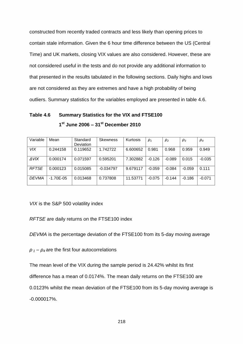
218

constructed from recently traded contracts and less likely than opening prices to

contain stale information. Given the 6 hour time difference between the US (Central

Time) and UK markets, closing VIX values are also considered. However, these are

not considered useful in the tests and do not provide any additional information to

that presented in the results tabulated in the following sections. Daily highs and lows

are not considered as they are extremes and have a high probability of being

outliers. Summary statistics for the variables employed are presented in table 4.6.

Table 4.6 Summary Statistics for the VIX and FTSE100

1st June 2006 – 31st December 2010

Variable Mean Standard Deviation

Skewness Kurtosis ρ1 ρ2 ρ3 ρ4

VIX 0.244158 0.119652 1.742722 6.600652 0.981 0.968 0.959 0.949

ΔVIX 0.000174 0.071597 0.595201 7.302882 -0.126 -0.089 0.015 -0.035

RFTSE 0.000123 0.015085 -0.034797 9.679117 -0.059 -0.084 -0.059 0.111

DEVMA -1.70E-05 0.013468 0.737808 11.53771 -0.075 -0.144 -0.186 -0.071

VIX is the S&P 500 volatility index

RFTSE are daily returns on the FTSE100 index

DEVMA is the percentage deviation of the FTSE100 from its 5-day moving average

ρ 1 – ρ4 are the first four autocorrelations

The mean level of the VIX during the sample period is 24.42% whilst its first

difference has a mean of 0.0174%. The mean daily returns on the FTSE100 are

0.0123% whilst the mean deviation of the FTSE100 from its 5-day moving average is

-0.000017%.

219

Autocorrelation is present for the VIX and for the deviation of the FTSE100 from its

5-day moving average. Autocorrelation is present but less strong for the first

difference of the VIX and for the FTSE100 returns. These results are fairly

unsurprising; in particular we would expect volatility indexes to be autocorrelated as

volatility is typically characterised by clustering. The high levels of skewness and

kurtosis indicate non-normality and provide further support for the presence of

autocorrelation and heteroskedasticity. Appropriate adjustments will therefore be

made in the empirical tests. The models to be estimated will focus on three key

issues. It is important to establish how the VIX responds to positive and negative

FTSE returns and deviations from its 5-day moving average in order to assess

whether it acts as a fear gauge22 for the UK market. Lagged VIX returns are also

included as an explanatory variable and the model is run for the entire sample

period, the pre-crisis period, crisis period and post-crisis period. Secondly, the

predictive power of the VIX for actual volatility in the UK will be analysed and

compared to that of time-varying volatility models such as GARCH and EWMA.

Finally tests will be constructed to examine the impact of the lagged VIX on

aggregate UK stock market returns in the pre-crisis period and the immediate

aftermath. The pre-crisis period is defined as above although a shorter crisis period

will be examined for the remainder of 2007.

4.4.3 Methodology

The initial step is to establish the relationship between aggregate market returns and

implied volatility by running regression 4.5. It is hypothesised that the opposite

response of the VIX to negative and positive returns on the S&P 500 similar to those

22

Whaley (2000) coined the term ‘investor fear gauge’ in response to the observation that high levels of market

turmoil coincided with high levels of the VIX. The key relationship is that when the market falls the VIX rises

and vice versa.

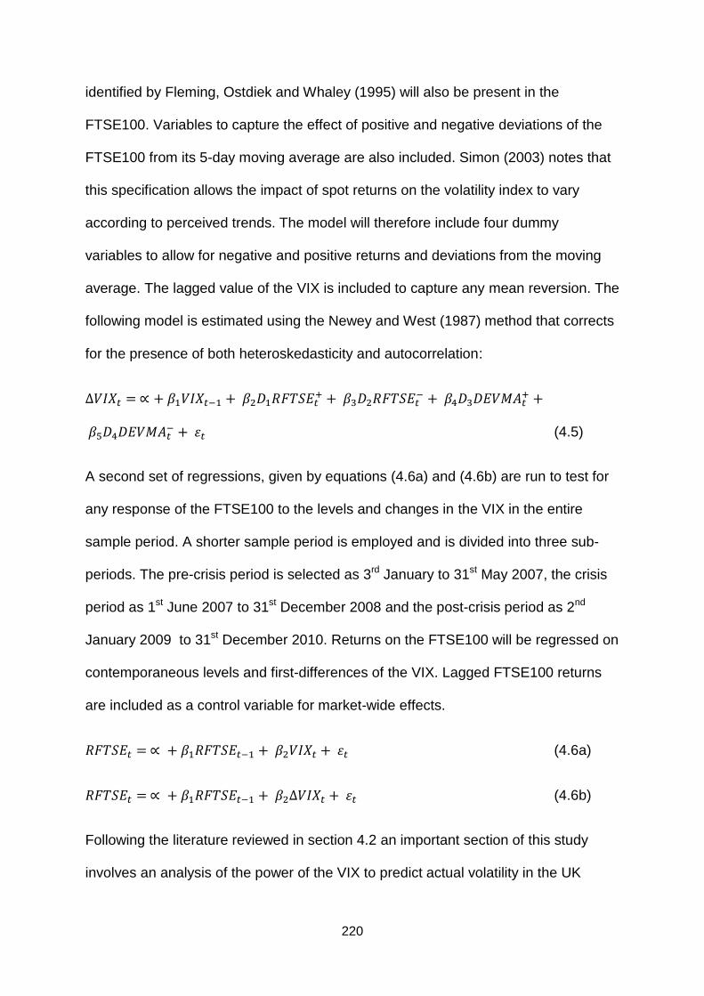
220

identified by Fleming, Ostdiek and Whaley (1995) will also be present in the

FTSE100. Variables to capture the effect of positive and negative deviations of the

FTSE100 from its 5-day moving average are also included. Simon (2003) notes that

this specification allows the impact of spot returns on the volatility index to vary

according to perceived trends. The model will therefore include four dummy

variables to allow for negative and positive returns and deviations from the moving

average. The lagged value of the VIX is included to capture any mean reversion. The

following model is estimated using the Newey and West (1987) method that corrects

for the presence of both heteroskedasticity and autocorrelation:

(4.5)

A second set of regressions, given by equations (4.6a) and (4.6b) are run to test for

any response of the FTSE100 to the levels and changes in the VIX in the entire

sample period. A shorter sample period is employed and is divided into three sub-

periods. The pre-crisis period is selected as 3rd January to 31st May 2007, the crisis

period as 1st June 2007 to 31st December 2008 and the post-crisis period as 2nd

January 2009 to 31st December 2010. Returns on the FTSE100 will be regressed on

contemporaneous levels and first-differences of the VIX. Lagged FTSE100 returns

are included as a control variable for market-wide effects.

(4.6a)

(4.6b)

Following the literature reviewed in section 4.2 an important section of this study

involves an analysis of the power of the VIX to predict actual volatility in the UK

221

market. A direct measure of the information content of option prices is the ability of

implied volatility to predict the future volatility of the underlying asset. Implied

volatility predictions will be compared with those produced by a GJR GARCH

(Glosten, Jaganathan and Runkle, 1993) model and an EWMA model. The use of a

GJR GARCH model is consistent with previous studies, such as Simon (2003), as it

picks up the frequently observed asymmetry in financial time series data. The value

of λ is chosen as 0.94 which is the appropriate value for daily index volatilities as

suggested by J.P. Morgan‟s RiskMetrics in 1994.

The GJR GARCH is designed to capture the asymmetric response of volatility to

news. In short, it is a typical characteristic of financial time series data that it

becomes more volatile in response to bad news than in response to good news of

equivalent magnitude. A standard GARCH (p,q) model does not capture this „stylised

fact‟. The asymmetric response can be illustrated in the following news impact curve

of the type proposed by Engle and Ng (1993):

Figure 4.3 GARCH News Impact Curves

ht

-ve +ve

222

The solid line represents the GARCH(1,1) whilst the dashed line represents the GJR

GARCH which dominates on the negative side of the diagram.

Initially the GJR GARCH model will be estimated in order to determine whether the

FTSE100 displays an asymmetric response of volatility to news. The model is

presented in equations (4.7a) and (4.7b):

( ) (4.7a)

(4.7b)

Where:

Rt = ln(Pt/Pt-1)

Pt = value of the FTSE100 index on day t

Dt-1 = 0 if εt-1 > 0, or Dt-1 = 1 otherwise

Hence the dummy variable magnifies the impact of the lagged innovation if it is

negative but the model collapses to a GARCH (1,1) if the lagged innovation is

positive. Hence this specification is capable of capturing the asymmetric response of

volatility to news. If is found to be statistically significant and positive then it can be

inferred that negative return innovations have a greater impact on the conditional

volatility of the FTSE100 than positive return innovations of the same magnitude.

Once more, predicted volatility will be analysed over the pre-crisis, crisis and post-

crisis periods as well as over the entire sample period.

223

Predictive Power of the VIX, GARCH and EWMA Forecasts for FTSE100

Volatility

In order to test the forecasting performance of the VIX it is compared to an out-of-

sample GJR GARCH over the period January 2007 to December 2010. As the model

is formulated to forecast one day ahead, a method similar to that of Lamoureux and

Lastrapes (1993) is adopted to transform GJR GARCH forecasts of daily variance to

forecasts of average daily variance for the remaining life of the relevant option

contract. The asymmetric GARCH parameters are estimated from FTSE100 returns

over the two year period which immediately precedes the forecasting period. An out-

of-sample model is used to produce estimates of volatility for day t+1 and is rolled

over for each subsequent day to produce a series of estimates up to day n where n

is one week prior to the maturity of the option. The average of these volatility

estimates is taken as the market consensus of volatility for the period under

consideration.

Finally the forecasting power of the VIX and GJR GARCH is compared with that of

the following EWMA model with λ set equal to 0.94:

( ) (4.8)

The remaining analysis in this section involves an adaptation of the methodology set

out in Simon (2003). In order to establish whether the VIX has predictive power in

relation to UK aggregate market return volatility a number of regressions are run

using levels and first differences. The predictive power of the VIX is compared to that

of the GARCH and EWMA models. The first of these regressions are in the levels

and are given by equation (4.9).

224

(4.9)

Where,

ζt, = the actual volatility of FTSE100 returns from 22 trading days before the nearest

to maturity option expiration through expiration.

ζVIX, ζG, ζEWMA = VIX, GARCH and EWMA forecasts of actual volatility measured 22

trading days prior to expiration of the nearest to maturity option.

The regression model in first differences is given by equation (4.10).

[ ] (4.10)

In equation 4.10 the dependent variable is the change in actual FTSE100 volatility

over the 22 days prior to the previous option expiration to the 22 days prior to the

nearest to maturity option expiration. The explanatory variable is the change in

actual volatility predicted by the VIX, GARCH or EWMA from its level prior to the

previous option expiration.

Consistent with Blair, Poon and Taylor (2001), Giot (2005) and Frijns, Tallau and

Tourani-Rad (2010) the actual or realised volatility is computed as the sum of the

squared daily returns. This is presented in equation (4.11):

√∑

(4.11)

Each model will indicate whether or not the volatility forecasts are biased. For an

unbiased forecast, the value of should not be significantly different to zero and the

slope coefficients should not be significantly different to one. For a volatility forecast

225

to have predictive power the coefficients attached to the volatility forecast in each

regression should be significantly greater than zero. In addition, Wald tests are

performed to test the joint restrictions that each intercept is equal to zero and that the

coefficient attached to each of the volatility forecasts is equal to one.

A further set of regressions is run in levels and first differences to establish whether

the information provided by the GARCH or EWMA forecasts is included in the VIX.

Equations (4.12a) for the levels and (4.12b) for first differences represent the

regression of actual FTSE100 volatility on the VIX and either the GARCH or the

EWMA volatility forecasts.

(4.12a)

[ ] [

] (4.12b)

If the information provided by the GARCH and EWMA volatility forecasts is contained

in the VIX then the coefficients attached to these forecasts should not be statistically

significant whilst the coefficients attached to the VIX should be statistically

significant. Likewise if information provided by the VIX is contained in the GARCH

and EWMA forecasts then the coefficients attached to the VIX will not be statistically

significant.

Predictive Power of the VIX for FTSE 100 Returns

A further test is run to investigate whether the VIX has any predictive power for

FTSE100 returns. If lagged values of the VIX, in levels or returns, are negatively and

significantly related to FTSE100 returns then the inference may be drawn that, if

investor expectations are incorporated into implied volatility, options markets have

predictive power for equity market returns. The regressions given by equations

(4.13a) and (4.13b) will be used to test this proposition.

226

(4.13a)

(4.13b)

The equation is specified for 22 lags although models with 1, 7 and 14 day lags will

also be analysed. The selection of lags is important as 22 working days is consistent

with the forward-looking horizon of implied volatility. The 1-day lag test examines for

the presence of price discovery with intermediate lags examined for completeness.

4.4.4 Results

The results from regression 4.5 are presented in table 4.7

Table 4.7 Model of daily changes in the VIX

Variable Whole Period Pre-Crisis Crisis Post-Crisis

Α -0.012512*** (0.0062)

0.183901*** (0.0074)

0.014446* (0.0691)

0.026154*** (0.0042)

β1 -0.101582*** (0.0000)

-1.541497*** (0.0085)

-0.096575*** (0.0015)

-0.169199*** (0.0000)

β 2 -1.214738*** (0.0002)

-1.695082 (0.3686)

-0.943129** (0.0123)

-1.227084** (0.0278)

β 3 -3.592918*** (0.0000)

-5.534605 (0.2634)

-3.293195*** (0.0000)

-4.042293*** (0.0000)

β 4 0.942115 (0.1131)

0.816662 (0.7880)

0.894682 (0.3192)

1.494741* (0.0693)

β 5 1.677950 (0.4793)

-5.846116 (0.3970)

1.308756 (0.2740)

-1.130183 (0.4550)

R2 0.267450 0.258229 0.283649 0.327680 Figures in parentheses are p-values. *** significant at the 1% level; ** significant at the 5% level, * significant at the 10% level.

It is apparent that for the whole sample period and each sub-period that the VIX

displays mean-reversion as each value of β1 is negative. Each coefficient estimate

on the lagged VIX return is negative and significant. Therefore a higher level of the

VIX is associated with a subsequent decline and vice versa. The coefficients on the

227

negative and positive lagged FTSE100 returns are also negative and significant,

except for during the pre-crisis period, indicating that positive lagged returns on the

FTSE100 are associated with declines in the VIX whilst negative lagged FTSE100

returns are associated with increases in the VIX. However these results should be

interpreted with caution because if, as expected, the VIX is moving in the opposite

direction to the US aggregate market then what is observed here could merely be a

result of correlation between the US and UK large capitalisation stock markets. It is

also important to note that the „contemporaneous‟ values for the VIX are also lagged

by six hours given the time difference between London and Chicago. Coefficients

attached to deviations of the FTSE100 from its 5-day moving average are not

statistically significant in both the whole period and each sub-period other than for

positive deviations in the post-crisis period, hence no inferences can be drawn about

these. The main conclusion to draw from this analysis is that the VIX moves in

opposite directions relative to the UK large capitalisation stock market. However the

primary relationship is with the US equity market. It follows that the evidence

supporting the notion of the VIX as a proxy fear gauge for the UK market is relatively

weak. Given the relationship between the UK and US equity markets it is

unsurprising that a highly directional relationship is identified.

228

Table 4.8 FTSE100 Returns and the VIX Levels and First-Differences

Levels Variable Whole Period Pre-Crisis Crisis Post-Crisis

Α 0.003804*** (0.0065)

0.012498** (0.0206)

0.003412 (0.2038)

0.006613*** (0.0045)

β1 -0.070820** (0.0448)

-0.026112 (0.7982)

-0.100271* (0.0651)

-0.027755 (0.4809)

β2 -0.015034** (0.0221)

-0.092191** (0.0398)

-0.015534 (0.1690)

-0.021921** (0.0213)

R2 0.017561 0.062568 0.020576 0.020871

First-Differences Variable Whole Period Pre-Crisis Crisis Post-Crisis

Α 0.000144 (0.6392)

0.000691 (0.2119)

-0.000593 (0.3399)

0.000507 (0.2686)

β1 -0.023848 (0.3786)

0.064261 (0.6450)

-0.035573 (0.3479)

-0.006917 (0.8693)

β2 -0.101020*** (0.0000)

-0.036333*** (0.0000)

-0.119779*** (0.0000)

-0.104705*** (0.0000)

R2 0.232138 0.146296 0.237117 0.272819 *** significant at the 1% level; ** significant at the 5% level, * significant at the 10% level. Figures in parentheses are p-values.

The most striking feature of the results in table 4.8 is the significant inverse

relationship between the first-difference of the VIX and the FTSE100. The VIX in the

level is less important as the VIX is non-stationary hence results are likely to be

misleading. The first-difference results suggest that the VIX is a useful indicator of

investor sentiment in the UK market. When investors are concerned in times of

falling returns the VIX rises; hence the VIX lives up to its reputation as a fear index.

This is particularly apparent when the model is run in first-differences and produces

coefficients that are all negative and significant. The negative coefficient attached to

the lagged VIX indicates that increasing volatility is associated with a subsequent fall

in returns. The results are consistent by sub-period except for the crisis period in the

levels.

229

Table 4.9 Asymmetric GARCH Model of Daily FTSE100 Returns

( )

Period

Entire 0.0000028*** (0.0000)

-0.013927 (0.3411)

0.188046*** (0.0000)

0.904380*** (0.0000)

Pre-Crisis 0.00000397*** (0.0000)

-0.233824*** (0.0000)

0.298379*** (0.0000)

1.00584*** (0.0000)

Crisis 0.0000102*** (0.0001)

-0.053287** (0.0291)

0.323583*** (0.0000)

0.870266*** (0.0000)

Post-Crisis 0.00000328*** (0.0020)

-0.030228 (0.1278)

0.162253*** (0.0000)

0.924778*** (0.0000)

Figures in parentheses are p-values. ***Significant at the 1% level **Significant at the 5% level

The results displayed in Table 4.9 provide support for the notion of asymmetric

volatility in response to innovations of equivalent magnitude but opposite sign. The

significant and positive value of for the entire period indicates that the news effect

is asymmetric. Notably the news effect is most prominent in the crisis and pre-crisis

periods. In particular, during the crisis period, negative innovations result in

considerable increases in conditional volatility. The value of is insignificant in the

pre-crisis and crisis periods, however if the model is run as a standard GARCH (1,1)

the influence of the lagged innovation becomes significant. The results also indicate

that conditional volatility is mean-reverting for all periods.

Tables 4.10 and 4.11 contain the regression results from equations (4.9) and (4.10)

and is based on 47 observations over the period from January 2007 to December

2010.

230

Table 4.10 The Predictive Power of Volatility Forecasts (Levels)

Constant VIX GARCH EWMA R2 D-W Wald Test

-0.002877** [0.001107]

0.516515*!

[0.089009] 0.275057 1.35 56.937

(0.0000)

-0.003512** [0.001599]

0.724681*!

[0.184368] 0.426721 1.93 79.02

(0.0000)

-0.002531** [0.001208]

0.572193*! [0.120957]

0.273363 1.62 41.358 (0.0000)

-0.003117** [0.001205]

-0.088156 [0.284704]

0.808352*** [0.435874]

0.429045 1.96

-0.003009** [0.001152]

0.278611 [0.167417]

0.284019 [0.250889]

0.284056 1.49

The Newey-West correction for autocorrelation and heteroskedasticity is used in the estimation and figures in parentheses are standard errors. * Significantly different from zero at the 10% level; ** at the 5% level. *** at the 1% level. The Wald test is for the joint hypothesis that the intercept is equal to zero and that the coefficient attached to the volatility estimate is equal to one. The Wald F-statistic is reported and probability values for the test are in parentheses.

! Significantly different from one.

The results presented in Table 4.10 indicate that the intercept coefficients in each

case are significantly less than zero. Furthermore in all cases, except for that where

GARCH and VIX volatility forecasts are jointly included in the model, the slope

coefficients are significantly less than one indicating that the volatility forecasts are

biased estimates of actual volatility. The results indicate that the VIX, GARCH and

EWMA volatility forecasts all have significant forecasting power. The combination of

a slope coefficient which is significantly greater than zero but significantly less than

one and an intercept which is significantly less than zero indicates that when volatility

forecasts are high relative to recent volatility their predictions of future volatility are

too high. The VIX and EWMA forecasts each explain approximately 27% of the

overall variation in the level of realised volatility whilst the GARCH forecast explains

approximately 43%. The model estimated including the GARCH and VIX forecasts

produces a GARCH coefficient which is not significantly different from one and an

insignificant coefficient for the VIX. This suggests that the GARCH encompasses the

231

forecasting information provided by the VIX. When the EWMA and VIX forecasts are

included both slope coefficients become insignificant. Hence in all cases it is not

possible to conclude that the information provided by the GARCH and EWMA

volatility forecasts is contained in the VIX.

Table 4.11 The Predictive Power of Volatility Forecasts (First Differences)

[ ]

Constant VIX GARCH EWMA R2 D-W Wald Test

-0.003645 [0.005246]

0.335981!

[0.403226] 0.046136 2.09 116.287

(0.0000)

-0.006446*** [0.002331]

0.919404*** [0.306324]

0.252161 2.19 25.435 (0.0000)

-0.003400 [0.007766]

0.39409!

[0.799395] 0.026736 2.25 61.953

(0.0000)

-0.005879 [0.004270]

-0.083846 [0.361270]

0.969166*** [0.344148]

0.254296 2.25

-0.003535 [0.007878]

0.354077** [164455]

-0.035416 [0.863421]

0.046218 2.09

The White correction for heteroskedasticity is used in the estimation and figures in parentheses are standard errors. * Significantly different from zero at the 10% level; ** at the 5% level. *** at the 1% level. The Wald test is for the joint hypothesis that the intercept is equal to zero and that the coefficient attached to the volatility estimate is equal to one. The Wald F-statistic is reported and probability values for the test are in parentheses.


The results in Table 4.11 show that the GARCH forecast by itself has a significantly

positive coefficient which is not significantly different from one, however the intercept

is significantly negative. Hence the GARCH forecast produces biased predictions of

actual volatility changes. When GARCH estimates are high relative to recent realised

volatility they over-predict rising volatility. The GARCH forecast explains

approximately 25% of the overall variation in realised volatility changes but the

coefficients attached to the VIX and EWMA forecasts are not significantly different to

zero.

232

When both the GARCH and VIX forecasts are included in the model the GARCH

continues to enter with a significantly positive coefficient whilst the VIX remains

insignificant. Hence the overall results are unchanged. Interestingly when the EWMA

and VIX are included the VIX volatility forecast becomes significantly greater than

zero although it only explains approximately 4.6% of the overall variation in realised

volatility changes.

Overall these results suggest that the GARCH model provides the most powerful

prediction of realised volatility. It provides significant predictive power both in levels

and first differences although the results also indicate that GARCH gives a biased

forecast of realised volatility. Furthermore, although significant in the levels, the

forecasting power of the EWMA and VIX is considerably weaker and insignificant

when combined with GARCH and in first-differences.

The VIX and FTSE100 Return Predictability

Potential return predictability is examined using equations (4.13a) and (4.13b) for a

variety of lag lengths denoted by the letter n. Results are presented in tables 4.12,

4.13 and 4.14.

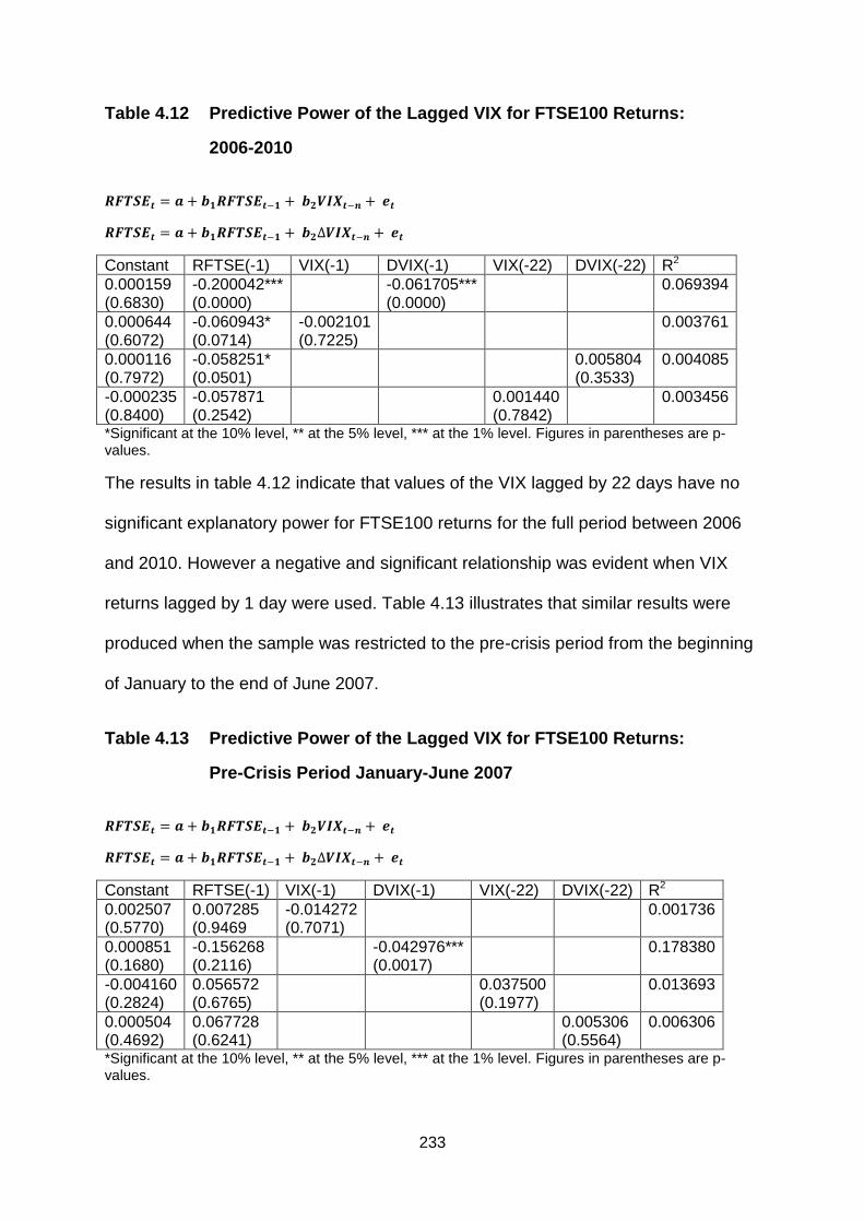
233

Table 4.12 Predictive Power of the Lagged VIX for FTSE100 Returns:

2006-2010

Constant RFTSE(-1) VIX(-1) DVIX(-1) VIX(-22) DVIX(-22) R2

0.000159 (0.6830)

-0.200042*** (0.0000)

-0.061705*** (0.0000)

0.069394

0.000644 (0.6072)

-0.060943* (0.0714)

-0.002101 (0.7225)

0.003761

0.000116 (0.7972)

-0.058251* (0.0501)

0.005804 (0.3533)

0.004085

-0.000235 (0.8400)

-0.057871 (0.2542)

0.001440 (0.7842)

0.003456

*Significant at the 10% level, ** at the 5% level, *** at the 1% level. Figures in parentheses are p-values.

The results in table 4.12 indicate that values of the VIX lagged by 22 days have no

significant explanatory power for FTSE100 returns for the full period between 2006

and 2010. However a negative and significant relationship was evident when VIX

returns lagged by 1 day were used. Table 4.13 illustrates that similar results were

produced when the sample was restricted to the pre-crisis period from the beginning

of January to the end of June 2007.


Pre-Crisis Period January-June 2007

Constant RFTSE(-1) VIX(-1) DVIX(-1) VIX(-22) DVIX(-22) R2

0.002507 (0.5770)

0.007285 (0.9469

-0.014272 (0.7071)

0.001736

0.000851 (0.1680)

-0.156268 (0.2116)

-0.042976*** (0.0017)

0.178380

-0.004160 (0.2824)

0.056572 (0.6765)

0.037500 (0.1977)

0.013693

0.000504 (0.4692)

0.067728 (0.6241)

0.005306 (0.5564)

0.006306


234

The model was also run with the VIX in the levels and first-differences with lags of

seven and fourteen days however no significant explanatory power was found.

A much shorter pre-crisis period which consisted of the 30 days prior to July 2007

was also examined. Again the results failed to provide significant evidence of return

predictability other than for the VIX lagged by seven days. Hence this result is

presented in Table 4.14 for completeness.


Short Pre-Crisis Period May/June 2007

Constant RFTSE(-1) VIX(-7) DVIX(-7) VIX DVIX R2

0.025489* (0.0630)

0.261432 (0.1688)

-0.183032* (0.0543)

0.119175

0.000153 (0.9050)

0.151328 (0.4034)

0.014446 (0.4565)

0.061439

0.009010 (0.3522)

0.181844 ((0.3267)

-0.061028 (0.3554)

0.062242

0.000333 (0.7919)

0.203641 (0.2576)

-0.022339 (0.1562)

0.113471


The weak results relating to lag lengths of greater than 1 day are likely to either be

because investor sentiment captured by volatility indexes cannot be used as a

predictor of aggregate market returns or, alternatively, the VIX is an inappropriate

proxy for investor sentiment in the UK large capitalisation equity market. The

significance of changes in the VIX lagged by 1 day indicate that there may be a

mechanism for price discovery in option trading data which warrants further

investigation.

235

4.4.5 Conclusion

The results presented in the preceding sections indicate that the VIX provides a

useful indicator of investor sentiment. Despite representing implied volatility of

S&P500 options, initial inspection appears to indicate that the VIX has some value

as a proxy for investor sentiment in the UK aggregate large capitalisation stock

market. Furthermore, the VIX appears to possess forecasting power for future

realised FTSE100 return volatility. However, this finding should be interpreted with a

considerable degree of caution because the forecasting power of the VIX disappears

with the inclusion of conditional GARCH volatility in the model. This is unsurprising

as the GARCH model produces estimates using UK data and also incorporates time-

varying volatility. No significant predictive power of the VIX for FTSE100 returns is

found. All of the results presented remain fairly consistent across the three sub-

periods of the financial crisis. This indicates that there was no major change in the

behaviour of options market traders as the crisis evolved. Or at least no major

change in trader behaviour can be implied from this data set.

Both the VIX and the VFTSE demonstrate clear mean-reversion. Furthermore, as

expected, there is a negative relationship between the VUK and the FTSE100 index.

Implied volatility increases when the market falls and decreases when the market

rises.

Given the results of the analysis of return predictability it would be inappropriate to

draw any strong inferences regarding the relationship between the VIX and

FTSE100 returns other than the VIX seems an inappropriate proxy for investor

sentiment in the UK market for the period and sub-periods analysed. At best it

236

indicates a weak price discovery mechanism. Consequently it is necessary to

employ an alternative approach in the search for further insights.

237

4.5 The VUK and the UK Equity Market Before and During the Financial Crisis

4.5.1 Introduction

As a consequence of the (lack of) strength of the results in the previous section it is

difficult to present a compelling argument for the relationship between the VIX and

returns in the UK equity market. In order to further examine the relationship between

implied volatility and spot asset returns, options market data will be used to construct

an ex ante VFTSE which may be used to model the sentiment of investors in the UK

prior to 2008. Henceforth this will be referred to as the VUK. The VUK will be

constructed in a similar way to the VFTSE in order to be a consistent indicator of

investor sentiment. This represents a unique contribution to the literature as it

permits examination of a series which did not previously exist.

Areal (2008) examined three different methodologies to produce the VFTSE in order

to find the preferred measure. Areal notes that the UK options market, although

liquid, is not as liquid as that in the US. For example, most of the liquidity in the UK

market is in close-to-the-money or at-the-money options. Hence it is inappropriate to

construct a volatility index using an identical measure to that used to produce the

VIX. As this study requires computation of an historical VUK index, an adaptation of

Areal‟s measure, which focuses on near-the-money options, will be employed.

4.5.2 Data

Data is collected to compute implied volatilities for the eight nearest-to-the-money

option contracts. These options are two puts and two calls for the nearest to

expiration and two puts and two calls for the second-nearest to expiration contracts.

238

Daily closing prices for FTSE100 European-style options, with their associated

exercise prices, for close-to-the-money contracts with the nearest two maturity dates

are collected from Euronext LIFFE. The entire sample period is from January 2006 to

December 2010, a total of 1,232 observations. This is a longer period than that

analysed in the previous section in order to compensate for the missing observations

from the Euronext LIFFE data noted below. Consequently the previous computations

on spot index data are repeated to ensure consistency. During the sample period the

expiry date of options traded on LIFFE was the third Friday of the month or the

previous working day if the Friday was a public holiday. The computations are

performed excluding options with less than one week to maturity. This addresses the

problems of low liquidity in close to expiration options and the high volatility

associated with imminent exercise or expiry.

FTSE100 index closing prices and dividend yields are collected from Datastream for

the entire sample period. There is no apparent consensus on the selection of an

appropriate riskless rate of interest to include in the option pricing model. For

example, Christensen and Prabhala (1998) assert that a one-month LIBOR rate

should be used as the risk-free rate as this is the rate most likely to be faced by

option traders. However numerous studies, including that of Areal (2008), suggest

some matching of the interest rate to the maturity of the option. Daily UK Treasury-

Bill rates for maturities closest to those of the options under consideration, collected

from Datastream, are used for the purposes of this study as they facilitate a

reasonable degree of maturity matching.

239

Table 4.15 Summary Statistics for the VUK and FTSE100

2nd January 2006 – 31st December 2012


Skewness Kurtosis ρ1 ρ2 ρ3 ρ4

VUK 0.188631 0.098100 2.054628 8.659449 0.953 0.922 0.904 0.892

ΔVUK 0.0000307 0.029821 -0.605756 21.13307 -0.167 -0.138 -0.076 0.029

RFTSE 0.0000494 0.014880 -0.060720 9.841489 -0.083 -0.050 -0.064 0.117

DEVMA -0.0000119 0.013245 0.820014 11.39718 -0.097 -0.114 -0.188 -0.071

VUK is the FTSE100 volatility index

RFTSE are daily returns on the FTSE100 index

DEVMA is the percentage deviation of the FTSE100 from its 5-day moving average

ρ 1 – ρ4 are the first four autocorrelations

The mean level of the VUK during the sample period is 18.86% whilst its first

difference has a mean of 0.00307%. Hence the implied volatility extracted from

FTSE 100 options in levels and first differences is considerably below that given by

the VIX. This is to be expected given the relationship between the VIX and the

VFTSE illustrated in Figure 4.2. Mean daily returns on the FTSE100 are 0.0049%

and the mean deviation of the FTSE100 from its 5-day moving average is -0.0019%.

Autocorrelation is present for the VUK, first difference of the VUK, FTSE100 returns

and the deviation of the FTSE100 from its 5-day moving average. Again these

results are fairly unsurprising. The high levels of kurtosis provide further support for

the presence of autocorrelation and heteroskedasticity. Appropriate adjustments will

therefore be made in the empirical tests which will focus on the same key issues

examined in section 4.4.

240

4.5.3 Methodology

The Black-Scholes-Merton model for options with a continuous dividend yield, as

presented and explained in Chapter 3, is used to extract a series of implied

volatilities for each of the option contracts in the sample. Implied volatilities are

calculated by setting the Black-Scholes price equal to the market price for each

option and solving for volatility for each of the 10,136 option prices in the sample.

The interpolation procedure presented in equation (4.14) is followed to produce at-

the-money implied volatilities for nearest and second-nearest to expiration put and

call options. This example uses notation for nearest to expiration puts.

(

)

(

)

(

)

(4.14)

Where:

S = price of the underlying asset

K = option exercise price

= implied volatility

The same procedure is applied to produce p,S-N, c,N and c,S-N.

The implied volatility for the nearest and second nearest to expiration contracts is

then computed by averaging that of the corresponding puts and calls as illustrated in

equations (4.15a) and (4.15b).

( ) (4.15a)

( ) (4.15b)

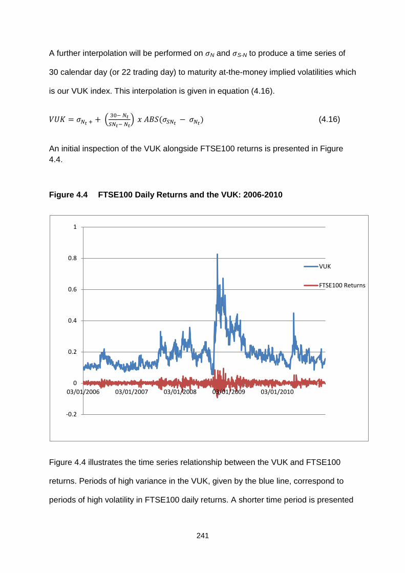
241

A further interpolation will be performed on N and S-N to produce a time series of

30 calendar day (or 22 trading day) to maturity at-the-money implied volatilities which

is our VUK index. This interpolation is given in equation (4.16).

(

) ( ) (4.16)

An initial inspection of the VUK alongside FTSE100 returns is presented in Figure

4.4.

Figure 4.4 FTSE100 Daily Returns and the VUK: 2006-2010

Figure 4.4 illustrates the time series relationship between the VUK and FTSE100

returns. Periods of high variance in the VUK, given by the blue line, correspond to

periods of high volatility in FTSE100 daily returns. A shorter time period is presented

-0.2

0

0.2

0.4

0.6

0.8

1

03/01/2006 03/01/2007 03/01/2008 03/01/2009 03/01/2010

VUK

FTSE100 Returns

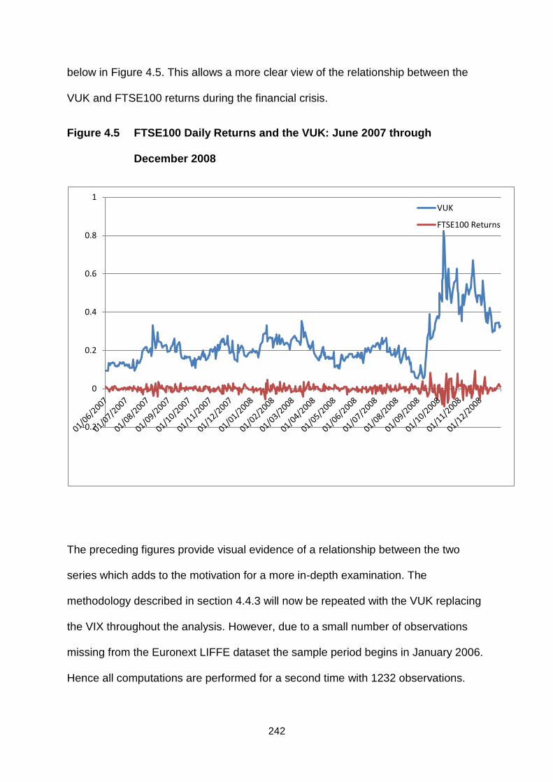
242

below in Figure 4.5. This allows a more clear view of the relationship between the

VUK and FTSE100 returns during the financial crisis.

Figure 4.5 FTSE100 Daily Returns and the VUK: June 2007 through

December 2008

The preceding figures provide visual evidence of a relationship between the two

series which adds to the motivation for a more in-depth examination. The

methodology described in section 4.4.3 will now be repeated with the VUK replacing

the VIX throughout the analysis. However, due to a small number of observations

missing from the Euronext LIFFE dataset the sample period begins in January 2006.

Hence all computations are performed for a second time with 1232 observations.

-0.2

0

0.2

0.4

0.6

0.8

1VUK

FTSE100 Returns

243

4.5.4 Results

Results from the regression presented in equation (4.2) are presented in table 4.16.

Table 4.16 Model of daily changes in the VUK

Variable Whole Period Pre-Crisis Crisis Post-Crisis

0.00739*** (0.0000)

0.024097*** (0.0075)

0.008763** (0.0164)

0.014507*** (0.0000)

β1 0.002620 (0.8626)

-0.165814** (0.0239)

0.011600 (0.6321)

-0.027913 (0.1169)

β 2 -1.787660*** (0.0000)

-2.001821*** (0.0000)

-2.168635*** (0.0000)

-1.266847*** (0.0000)

β 3 0.137884 (0.5057)

-0.326692 (0.1054)

0.229380 (0.5085)

0.329834* (0.0648)

β 4 0.322267 (0.2054)

0.030054 (0.9690)

0.488113 (0.2120)

-0.242473 (0.4850)

β 5 -0.574559 (0.1320)

-1.008977** (0.0336)

-1.132080** (0.0426)

0.274088 (0.5961)

R2 0.282543 0.473045 0.409652 0.150857 Figures in parentheses are p-values. *** significant at the 1% level; ** significant at the 5% level, * significant at the 10% level.

The results presented in Table 4.16 provide useful insights. Positive changes in the

FTSE100 are strongly linked to negative changes in the VUK. This indicates that

when stock returns are high the VUK volatility index falls. Except for the post-crisis

period, the coefficients attached to negative changes in the FTSE100 are not

statistically significant. These results suggest that the VUK responds asymmetrically

to positive and negative contemporaneous returns. This is in sharp contrast to the

findings of Simon (2003) on the VXN. Interestingly, during the crisis and pre-crisis

periods the results are reversed. Positive deviations of the FTSE100 from its 5-day

moving average are insignificant whereas negative deviations from its 5-day moving

average are negative and significant. One interpretation of this result is that, when a

negative trend is perceived during a predominantly falling market, demand for

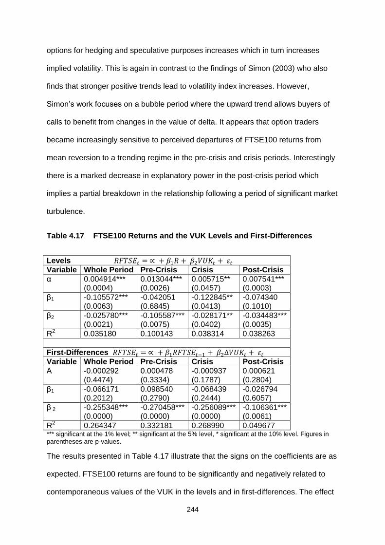
244

options for hedging and speculative purposes increases which in turn increases

implied volatility. This is again in contrast to the findings of Simon (2003) who also

finds that stronger positive trends lead to volatility index increases. However,

Simon‟s work focuses on a bubble period where the upward trend allows buyers of

calls to benefit from changes in the value of delta. It appears that option traders

became increasingly sensitive to perceived departures of FTSE100 returns from

mean reversion to a trending regime in the pre-crisis and crisis periods. Interestingly

there is a marked decrease in explanatory power in the post-crisis period which

implies a partial breakdown in the relationship following a period of significant market

turbulence.

Table 4.17 FTSE100 Returns and the VUK Levels and First-Differences

Levels Variable Whole Period Pre-Crisis Crisis Post-Crisis

α 0.004914*** (0.0004)

0.013044*** (0.0026)

0.005715** (0.0457)

0.007541*** (0.0003)

β1 -0.105572*** (0.0063)

-0.042051 (0.6845)

-0.122845** (0.0413)

-0.074340 (0.1010)

β2 -0.025780*** (0.0021)

-0.105587*** (0.0075)

-0.028171** (0.0402)

-0.034483*** (0.0035)

R2 0.035180 0.100143 0.038314 0.038263

First-Differences Variable Whole Period Pre-Crisis Crisis Post-Crisis

Α -0.000292 (0.4474)

0.000478 (0.3334)

-0.000937 (0.1787)

0.000621 (0.2804)

β1 -0.066171 (0.2012)

0.098540 (0.2790)

-0.068439 (0.2444)

-0.026794 (0.6057)

β 2 -0.255348*** (0.0000)

-0.270458*** (0.0000)

-0.256089*** (0.0000)

-0.106361*** (0.0061)

R2 0.264347 0.332181 0.268990 0.049677 *** significant at the 1% level; ** significant at the 5% level, * significant at the 10% level. Figures in parentheses are p-values.

The results presented in Table 4.17 illustrate that the signs on the coefficients are as

expected. FTSE100 returns are found to be significantly and negatively related to

contemporaneous values of the VUK in the levels and in first-differences. The effect

245

is much more powerful in first-differences indicating that it is the increase in implied

volatility rather than the level which is most strongly associated with negative returns

on the FTSE100 index. It is clear that the first-differenced series of the VUK is a

powerful tool for illustrating investor sentiment in the UK market and may be

regarded as an appropriate fear gauge. The VUK in the levels is less important and

may be misleading given that the VUK is non-stationary.23 Other than during the

crisis period the coefficient attached to the lagged FTSE100 returns is not significant.

Table 4.18 contains the regression results from running equations (4.9) and (4.12a)

and is based on 47 observations over the period January 2007-December 2010.

Table 4.18 The Predictive Power of Volatility Forecasts (Levels)

Constant VUK GARCH EWMA R2 D-W Wald Test

-0.004903*** [0.001373]

0.789057*** [0.168193]

0.353361 1.53 122.4324 (0.0000)

-0.003350*** [0.001034]

0.690128***! [0.132273]

0.451548 2.18 142.1537 (0.0000)

-0.00264*** [0.000909]

0.564585***! [0.107235]

0.312943 1.83 1657442 (0.0000)

-0.004023*** [0.000815]

0.137502 [0.204264]

0.600873**! [0.255426]

0.454726 2.12

-0.004750*** [0.001271]

0.631866***! [0.191217]

0.133058 [0.127044]

0.356719 1.60

The Newey-West correction for autocorrelation and heteroskedasticity is used in the estimation. Figures in parentheses are standard errors. * Significantly different from zero at the 10% level; ** at the 5% level. *** at the 1% level. The Wald test is for the joint hypothesis that the intercept is equal to zero and that the coefficient attached to the volatility estimate is equal to one. The Wald F-statistic is reported and probability values for the test are in parentheses.


The results presented in Table 4.18 indicate that the intercept coefficients in each

case are significantly less than zero. Furthermore, in the GARCH and EWMA

estimations the slope coefficients are significantly less than one. This indicates that

23

An Augmented Dickey Fuller test on the VUK with 3 lags gives a t-statistic of -3.438 and probability of

(0.000). The VUK is found to be stationary in first differences.

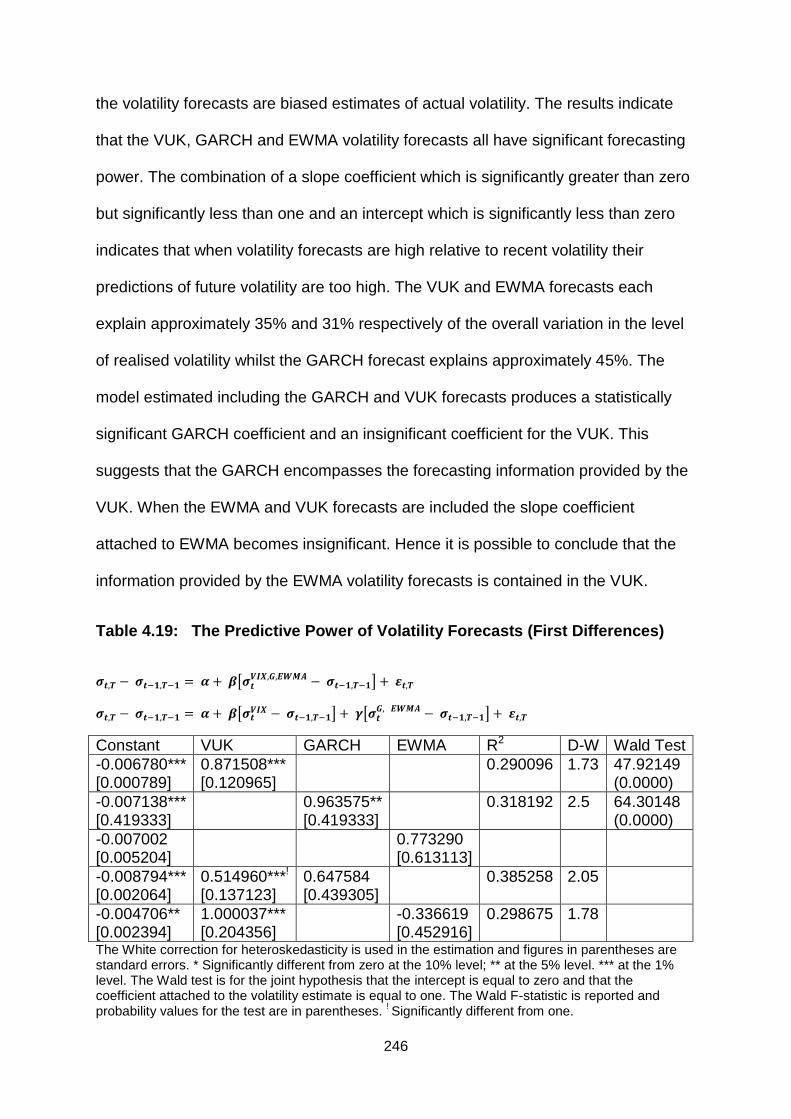
246

the volatility forecasts are biased estimates of actual volatility. The results indicate

that the VUK, GARCH and EWMA volatility forecasts all have significant forecasting

power. The combination of a slope coefficient which is significantly greater than zero

but significantly less than one and an intercept which is significantly less than zero

indicates that when volatility forecasts are high relative to recent volatility their

predictions of future volatility are too high. The VUK and EWMA forecasts each

explain approximately 35% and 31% respectively of the overall variation in the level

of realised volatility whilst the GARCH forecast explains approximately 45%. The

model estimated including the GARCH and VUK forecasts produces a statistically

significant GARCH coefficient and an insignificant coefficient for the VUK. This

suggests that the GARCH encompasses the forecasting information provided by the

VUK. When the EWMA and VUK forecasts are included the slope coefficient

attached to EWMA becomes insignificant. Hence it is possible to conclude that the

information provided by the EWMA volatility forecasts is contained in the VUK.

Table 4.19: The Predictive Power of Volatility Forecasts (First Differences)

[ ]

[ ] [

]

Constant VUK GARCH EWMA R2 D-W Wald Test

-0.006780*** [0.000789]

0.871508*** [0.120965]

0.290096 1.73 47.92149 (0.0000)

-0.007138*** [0.419333]

0.963575** [0.419333]

0.318192 2.5 64.30148 (0.0000)

-0.007002 [0.005204]

0.773290 [0.613113]

-0.008794*** [0.002064]

0.514960***!

[0.137123] 0.647584 [0.439305]

0.385258 2.05

-0.004706** [0.002394]

1.000037*** [0.204356]

-0.336619

[0.452916] 0.298675 1.78

The White correction for heteroskedasticity is used in the estimation and figures in parentheses are standard errors. * Significantly different from zero at the 10% level; ** at the 5% level. *** at the 1% level. The Wald test is for the joint hypothesis that the intercept is equal to zero and that the coefficient attached to the volatility estimate is equal to one. The Wald F-statistic is reported and probability values for the test are in parentheses.


247

The results in Table 4.19 show that the VUK and GARCH forecasts by themselves

have significantly positive coefficients which are not significantly different from one,

however the intercepts are significantly negative. Hence the VUK and GARCH

forecasts produce biased predictions of actual volatility changes. When these

estimates are high relative to recent realised volatility they over-predict rising

volatility. The GARCH forecast explains approximately 32% of the overall variation in

realised volatility changes and the VUK approximately 29%. However the coefficient

attached to the EWMA forecast is not significantly different to zero.

When both the GARCH and VUK forecasts are included in the model the VUK

continues to enter with a significantly positive coefficient whilst the GARCH becomes

insignificant. This is a reversal of the result found in the levels and suggests that in

first-differences the VUK encompasses the forecasting information provided by the

GARCH. When the EWMA and VUK are included the VUK volatility forecast remains

significant and explains approximately 30% of the overall variation in realised

volatility changes.

Overall these results suggest that the VUK and the GARCH model are powerful

predictors of realised volatility in the FTSE100 index. They provide significant

predictive power both in levels and first differences although the results also indicate

that the forecasts of realised volatility are biased. Furthermore, the forecasting power

of the EWMA is found to be insignificant in levels and in first-differences.

248

The VUK and FTSE100 Return Predictability

Potential stock market return predictability provided by the VUK is examined using

equations (4.13a) and (4.13b) for a variety of lag lengths. Results are presented in

table 4.20.

Table 4.20 Predictive Power of the Lagged VUK for FTSE100 Returns:

2006-2010

Constant RFTSE(-1) VUK(-1) DVUK(-1) VUK(-22) DVUK(-22) R2

0.001248 (0.4192)

-0.089339*** (0.0152)

-0.006371 (0.4919)

0.008574

0.0000557 (0.8851)

-0.199698*** (0.0001)

-0.138912*** (0.0006)

0.070539

-0.000656 (0.4819)

-0.083473*** (0.0037)

0.003612 (0.4076)

0.007403

0.0000313 (0.9420)

-0.083445*** (0.0037)

0.009753 (0.4974)

0.007221


Lagged values of the VUK were found to have no significant explanatory power for

FTSE100 returns regardless of the lag length selected for the full period between

2006 and 2010. However some weak explanatory power was found in the change in

the VUK lagged by one day. This suggests that options markets may be performing

a weak price discovery function. The results presented in Table 4.21 illustrate that

findings were broadly similar when the sample was restricted to the pre-crisis period

from the beginning of January to the end of June 2007.

249


Pre-Crisis Period January-June 2007

Constant RFTSE(-1) VUK(-1) DVUK(-1) VUK(-22) DVUK(-22) R2

-0.011948*** (0.0000)

0.110197 (0.1401)

0.119037*** (0.0000)

0.117704

0.000442 (0.3519)

0.218390** (0.0404)

0.1085882** (0.0421)

0.056033

0.001375 (0.6099)

0.084239 (0.2805)

-0.007539 (0.7348)

0.007498

0.000516 (0.3225)

0.083141 (0.2933)

-0.002044 (0.9559)

0.006668


The results are very similar to those found when the entire period is analysed. Again

there is evidence of price discovery in the lagged change in the VUK. However

during this period there is also some predictive power evident in the lagged VUK

index level.

The most plausible explanation of the relatively weak results presented above is that

a VUK volatility index has little value as an indicator of return predictability in the

underlying equity market and only limited value as a price discovery mechanism.

This explanation implies that professional options traders do not price future market

moves into contracts with any degree of accuracy. Hence implied volatility does not

provide a strong signal of crash expectations even during turbulent periods.

However, despite the financial crisis first breaking in 2007 no significant negative

returns were observed on the FTSE100 until mid-2008. It appears that the UK large

capitalisation equity market remained remarkably robust to these events for a

sustained time period. This is one possible contributory factor to the absence of a

significant relationship between the lagged UK volatility index and FTSE100 returns.

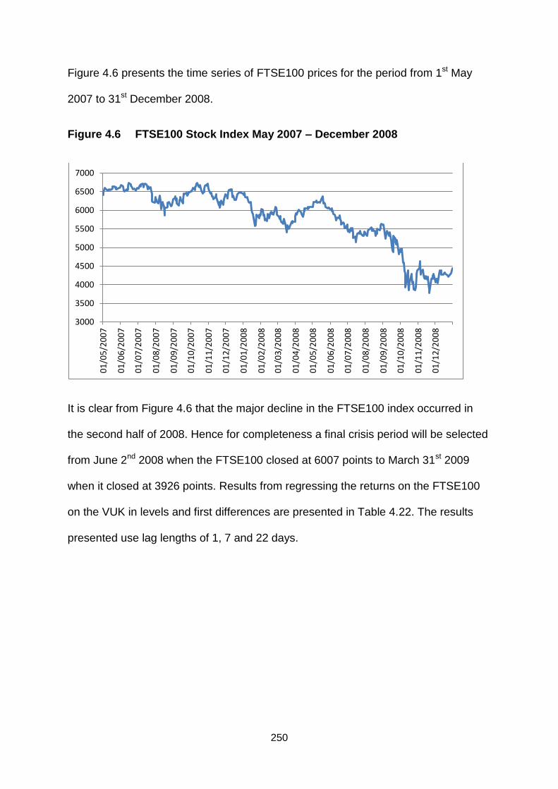
250

Figure 4.6 presents the time series of FTSE100 prices for the period from 1st May

2007 to 31st December 2008.

Figure 4.6 FTSE100 Stock Index May 2007 – December 2008

It is clear from Figure 4.6 that the major decline in the FTSE100 index occurred in

the second half of 2008. Hence for completeness a final crisis period will be selected

from June 2nd 2008 when the FTSE100 closed at 6007 points to March 31st 2009

when it closed at 3926 points. Results from regressing the returns on the FTSE100

on the VUK in levels and first differences are presented in Table 4.22. The results

presented use lag lengths of 1, 7 and 22 days.

3000

3500

4000

4500

5000

5500

6000

6500

7000

01

/05

/20

07

01

/06

/20

07

01

/07

/20

07

01

/08

/20

07

01

/09

/20

07

01

/10

/20

07

01

/11

/20

07

01

/12

/20

07

01

/01

/20

08

01

/02

/20

08

01

/03

/20

08

01

/04

/20

08

01

/05

/20

08

01

/06

/20

08

01

/07

/20

08

01

/08

/20

08

01

/09

/20

08

01

/10

/20

08

01

/11

/20

08

01

/12

/20

08

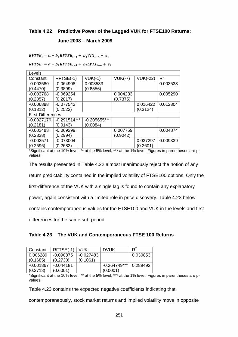
251


June 2008 – March 2009

Levels

Constant RFTSE(-1) VUK(-1) VUK(-7) VUK(-22) R2

-0.003580 (0.4470)

-0.064908 (0.3899)

0.003533 (0.8556)

0.003533

-0.003768 (0.2857)

-0.069254 (0.2817)

0.004233 (0.7375)

0.005290

-0.006888 (0.1312)

-0.077542 (0.2522)

0.016422 (0.3124)

0.012804

First-Differences

-0.0027176 (0.2181)

-0.291514*** (0.0143)

-0.205655*** (0.0084)

-0.002483 (0.2838)

-0.069299 (0.2994)

0.007759 (0.9042)

0.004874

-0.002571 (0.2596)

-0.073004 (0.2683)

0.037297 (0.2601)

0.009339


The results presented in Table 4.22 almost unanimously reject the notion of any

return predictability contained in the implied volatility of FTSE100 options. Only the

first-difference of the VUK with a single lag is found to contain any explanatory

power, again consistent with a limited role in price discovery. Table 4.23 below

contains contemporaneous values for the FTSE100 and VUK in the levels and first-

differences for the same sub-period.

Table 4.23 The VUK and Contemporaneous FTSE 100 Returns

Constant RFTSE(-1) VUK DVUK R2

0.006289 (0.1685)

-0.090875 (0.2730)

-0.027483 (0.1061)

0.030853

-0.001867 (0.2713)

-0.044181 (0.6001)

-0.264749*** (0.0001)

0.289492


Table 4.23 contains the expected negative coefficients indicating that,

contemporaneously, stock market returns and implied volatility move in opposite

252

directions. However statistical significance is only found when the first-difference of

the VUK is the explanatory variable. This is to be expected as the VUK, in common

with the VIX, is non-stationary. The information in Table 4.23 provides support for the

hypothesis that the VUK in first-differences performs a price discovery role for the

underlying FTSE 100 index.

4.5.5 Conclusion

The results in this section are made possible by the construction of a unique volatility

index that is used to draw meaningful inferences about the relationships between

volatility implied by FTSE 100 index option prices and the underlying equity index.

The relationships identified between contemporaneous FTSE100 stock index returns

and volatility indexes provide support for the conclusion of Whaley (2000) who finds

that they are representative of the sentiment of market participants. Volatility indexes

are found to provide a useful indication of future realised volatility. In general they

provide better predictions than an EWMA model and at least as good predictions as

an asymmetric GARCH model.

The results presented do not support the hypothesis that implied volatility indexes

provide an accurate prediction of future market returns. Hence there is no evidence

produced here that indicates an opportunity to earn consistent abnormal profits.

There is some evidence of a role of options in price discovery which motivates

further investigation in terms of trading volume and open interest. However there is

no evidence in this chapter of market inefficiency. In other words it cannot be inferred

that information about volatility is not being rapidly incorporated into prices.

Furthermore, results are found to be fairly consistent across each sub-period of the

financial crisis.

253

It is recognised that there are some limitations to the results which are governed by

the availability of UK options market data. The use of daily data poses a problem of

non-synchronisation given that the equity market and options market have different

closing times. Nevertheless, if the impact of non-synchronous prices is random then

the tests should be unbiased.

254

Chapter 5

An Analysis of Trading Volume and Open

Interest in UK FTSE100 Index and

Individual Equity Options Markets during

the 2007-2008 Financial Crisis

255

5.1 Introduction and Motivation

The motivation for this chapter is to build on the analysis presented in Chapter 4 by

undertaking an investigation of investor trading behaviour in FTSE100 index and

single equity options traded on LIFFE. More precisely, the relationship between the

aggregate large capitalisation market, financial stocks and options underlying the

index and the financial stocks will be examined in order to contribute to the debate

on the means by which information is incorporated into asset prices. The central

objective of this chapter is to establish whether any predictive power for financial

stock returns can be identified in options market trading behaviour and, if so, how

strong this relationship is.

Options are not necessarily redundant assets, even though their returns can be

replicated by employing a dynamic trading strategy which involves a combination of

stocks and riskless assets. The reason for this is that they can provide investors with

a low cost, leveraged alternative to taking an equity position and, furthermore, do not

suffer from the short-sales restrictions that are present in equity markets. So, in

incomplete markets where price is driven by trading, informed traders who take

advantage of this alternative will contribute to price discovery in equity markets.

Although the majority of studies do not find evidence of predictability at an aggregate

level during periods of relative tranquillity, it is nevertheless worthwhile to test for any

predictability (particularly using individual securities related to the financial sector)

during a period of significant financial turbulence. If significant predictive power can

be identified than this will pose a challenge for the efficient markets hypothesis,

albeit due to limited arbitrage.

256

It is intuitive to expect that an increase in call trading volume will be observed in

rising markets, as traders seek to benefit from greater leverage. Similarly when the

market is declining, more put trading volume is likely to occur as a result of

speculative or hedging demand aimed at overcoming short sales restrictions or

achieving portfolio insurance. It follows that pessimistic investor expectations should

result in an increase of trading in puts relative to that in calls. Again it is likely that

relatively fewer call positions will be opened for speculative purposes when investors

do not expect prices to rise with the consequent impact on relative trading volume.

Even though it is possible to profit from the time decay by writing call options the

purchase of puts provides a much more attractive opportunity. Furthermore, as

suggested by Simon (2003) the absolute impact on call trading volume is likely to be

tempered somewhat by the actions of risk-averse investors who view call options as

a low risk means of investing in stocks. Should investor expectations be particularly

pessimistic towards companies in the financial sector then the imbalance in trading

should be most pronounced in options written on the stocks of financial firms.

Net open interest provides an additional source of information on option trading

behaviour. Open interest indicates the number of option contracts which remain

outstanding at the close of each trading day. As option traders themselves write

options, open interest may be regarded as endogenous and therefore reflect the

beliefs and risk preferences of options traders. Beliefs and risk-preferences are both

factors that are prominent in the field of behavioural finance. Trading volume

comprises four components; opening a contract to buy, opening a contract to sell,

closing out a contract to buy and closing out a contract to sell. The last two

components reduce open interest, so on any given day an increase in trading

volume could have a net effect of either increasing or decreasing open interest. A

257

positive change in open interest indicates that more contracts are being opened than

are being closed out thus it provides a useful indicator of option trading behaviour.

However, open interest also has its limitations as it only measures the number of

contracts outstanding.

The contemporaneous relationship between relative trading volume/open interest

and index/equity portfolio returns will be also be examined for evidence of price

discovery. Furthermore, a behavioural approach will be formulated to isolate trading

behaviour in response to a series of return innovations of the same sign.

Daily trading volume and open interest of FTSE100 and single equity put and call

options traded in the UK options market are recorded by Euronext LIFFE. The index

options are European-style whilst the equity options are American-style. All of the

options in each category trade with a variety of strike prices and mature on the third

Friday of the delivery month. Time series of trading volume and open interest ratios

for index and single stock options will be analysed for the period 2006-2010 in an

attempt to detect any changes in behaviour to occur during this period and to identify

any predictive power that may be inferred from the data.

This chapter will examine and seek to address the following questions which are

related to those posed in Chapter 4:

Is there any significant predictive relationship between the relative trading

volume and open interest of put and call options written on the FTSE100 and

future spot market returns?

Is there any significant predictive relationship between the relative trading

volume and open interest of put and call options written on financial stocks

and future spot market returns?

258

Is it possible to infer any change in investor behaviour across each stage of

the financial crisis?

Is relative trading behaviour influenced by a series of return innovations of the

same sign?

5.2 Literature

There is seemingly little literature available that relates trading volume to crash

expectations although a number of studies have focused on the informational

content of trading volume and open interest during periods of relative tranquillity in

markets and during periods of relative turbulence.

Manaster and Rendleman (1982) produced one of the first investigations into market

expectations embedded into option prices. The purpose of this study was to

determine whether the options market responds more quickly than the stock market

to the arrival of new information. Manaster and Rendleman used daily data to

compute the stock price implied by the Black-Scholes model and compared this with

the market price. Their results indicated that the implied prices contain information

about future stock returns. However they are unable to establish whether traders

could use this information to earn excess returns.

Stephan and Whaley (1990) use intraday data on CBOE options from the first

quarter of 1986 to produce implied stock prices. They argue that intraday data

produces more reliable results as it overcomes the problem of non-

contemporaneous closing prices. The change in implied stock price is compared to

the change in the actual stock price to identify a lead-lag relationship. Stephan and

Whaley conclude that stock returns lead option returns by an average of about

fifteen to twenty minutes.

259

One important concern regarding tests of implied stock prices is that they are likely

to be sensitive to the method of volatility computation.

Figlewski and Webb (1993) investigate the role of CBOE options in improving

transactional and informational efficiency in the S&P500 stock market in the context

of short-selling restrictions. The relationship between short interest and stocks with

and without exchange-traded options is examined.24 Short interest should be higher

for stocks with options written on them because the puts can be used as an

alternative to short-selling by constrained investors. Market makers subsequently

take short positions to cover the options written, leading to higher short interest for

stocks with corresponding exchange-traded options. Figlewski and Webb

hypothesise that there should be positive correlation between short interest and the

difference between put and call implied volatilities. They conclude that the

relationships between short interest and exchange-traded options and between short

interest and implied volatilities indicates that option trading contributes to

transactional and informational efficiency in stock markets.

Mayhew, Sarin and Shastri (1995) analyse market microstructure and note that

option margin requirements play a role in efficiency because higher margins reduce

liquidity. This in turn decreases the rate of information flow to equity markets

because of the impact on arbitrage links, relative trading costs and investor

migration. In particular less-informed investors, who are assumed to be more capital

constrained, are likely to migrate in response to margin changes which in turn affects

relative concentration. Mayhew, Sarin and Shastri find evidence that supports

migration between markets and changes in relative concentration. They also note

24

Short interest is defined as the number of shares that have been sold short but not yet covered by

repurchasing.

260

that the 1986 decrease in margin on options traded on the CBOE increased

information to the stock market, but that the margin increase of 1998 resulted in no

change in the underlying market. The study has a behavioural aspect as it is

uninformed traders that are most sensitive to margin changes and are therefore key

to the results.

Amin and Lee (1997) examine the relationship between option trading volume and

firm-specific news and produce evidence of price discovery. Their sample contains

options traded on the CBOE in 1988 and 1989 with corresponding stock prices from

the New York and American stock exchanges. Amin and Lee present evidence of an

increase in option market activity up to four days prior to an earnings announcement

which is sustained for several days afterwards. Of course, the additional volume

could be a response to volatility risk or an opportunity for volatility speculation where

traders construct strategies such as straddles, strangles, strips and straps. However,

Amin and Lee find that the trading volume is directional as put option open interest

increased prior to negative earnings news and decreased prior to positive earnings

news. This finding implies that predictability may be found in open interest data

which in turn will be a reasonable proxy for private information. Furthermore, Amin

and Lee find that option traders also provide private information to the market during

non-announcement periods.

Easley, O‟hara and Srinivas (1998) also investigate the role of options in

informational efficiency where traders have heterogeneous information sets. They

find evidence to indicate a link between trading volume and stock returns, which is

independent of significant events in the market such as takeover announcements.

Stock price changes are found to lead options market trading volume but when

261

option trades are categorised as driven by good news or bad news they find that

trading volume provides information about future stock price changes.

Chakraverty, Gulen and Mayhew (2004) investigate the role of options in price

discovery using individual equity options traded on the CBOE between 1988 and

1992. They find that options do perform a price discovery function with the

information flow greatest when trading volume is high. The evidence of price

discovery does not imply that informed traders use their information to trade in

options markets although Chakraverty at al do not rule out the possibility of this

information being made public through the hedging decisions of informed market

makers. If spot market traders observe these „signals‟ then this would be akin to

trading on the basis of „inside‟ information which, if profitable, represents a violation

of the strong form of the efficient markets hypothesis.

Cao, Chen and Griffin (2005) investigate the informational content of trading volume

in CBOE options between 1986 and 1994 prior to merger and acquisition activity.

They find that the highest pre-announcement buyer-initiated call trading volume is

associated with the highest announcement day returns. This is interpreted as

informed options traders playing a key role in price discovery for extreme

informational events. Cao et al did find that trading volume of call options written on

firms prior to a takeover announcement had predictive power for the magnitude of

takeover premiums. Cao et al find little to suggest that option trading volume predicts

stock returns during periods when market behaviour is normal. This finding is

supported by Chan, Chung and Fong (2002) who find that option trading volume

provides no predictive power.

262

Pan and Poteshman (2006) investigate the information regarding future stock price

movements contained in the trading volume of CBOE options. The authors‟ data set

allows them to separate public information from that which is privately held and to

categorise option traders by degree of sophistication. They find that the trading

behaviour of informed traders demonstrates significant predictability for future stock

returns. The information provided by option trading volume is found to take several

weeks to be impounded into stock prices. However it is argued that this finding does

not contradict the efficient markets hypothesis simply because the information used

in the tests would not have been publicly available at the time. One interesting point

is that although informed trading is evident in the individual stock option market there

was no such evidence to be found in the index option market. This indicates that

informed investors do not have access to private information at an aggregate level.

Buraschi and Jiltsov (2006) examine S&P500 index option data under the

assumption that option market participants have heterogeneous beliefs. This is used

to establish an option pricing model under conditions of uncertainty. Importantly for

this study Buraschi and Jiltsov establish a link between these heterogeneous beliefs

and option market open interest. They demonstrate that a one standard deviation

increase in an index of heterogeneous beliefs results in a 20% increase in option

open interest. This study differs from previous work in that index options, where

trades are much less likely to be driven by private information, are considered.

Cao and Yang (2009) develop a theoretical model which considers traders with

heterogeneous beliefs and is extended to multiple periods. They find that public

information that is likely to result in investor disagreement has different implications

for participants in equity and options markets. Cao and Yang assert that trading

volume in equities increases in response to public news and diffuses slowly,

263

whereas option trading is clustered before and during the public news event. A

limitation of Cao and Yang‟s approach is that it excludes the possibility of investor

acquisition of private information.

Chang, Hsieh and Lai (2009) examine the Taiwan stock market for any evidence of

stock return predictability in option trading volume. In particular they investigate the

impact that option market activity of foreign investors has on domestic returns. It is

hypothesised that the high liquidity and low transactions costs in the options market

attract informed investors more than the related equity markets. It follows that activity

in the options market is likely to provide information on the future movement of the

underlying asset. Chang et al are unable to find any predictability for stock market

returns using aggregate trading volume or open interest lagged up to seven days.

However, when the data was disaggregated, strong predictive power was found in

the trading volume of foreign institutional investors.

5.3 Data

Daily trading volume and open interest of European-style FTSE100 index and

American-style individual equity put and call options are collected from Euronext

LIFFE. Stock prices of the financial companies underlying the individual equity

options are collected from Datastream. The financial stock portfolio consists of fifteen

stocks from the banking, financial services and insurance sectors. The stocks

selected correspond to those financial companies with associated options traded on

LIFFE. The list of companies with their LIFFE codes and sectors is presented in

Appendix 3. The sum of all put and call options traded on a given day are used to

construct the first series of trading volume and open interest ratios for the empirical

tests. However, following Pan and Poteshman (2006) out-of-the-money options are

264

also used for the empirical work in order to capture leverage effects. The rationale is

that, if an investor has private positive or negative information, greater leverage can

be achieved by purchasing out-of-the-money calls or puts respectively. Furthermore,

out-of-the-money options typically have higher trading volume than those in-the-

money. The combined effect is that any predictability of future returns is likely to be

most evident in results produced from analysis of out-of-the-money options.

Data on the FTSE100, to be employed in the analysis that follows, is the same set as

that used in the previous chapter. Additional stock price data on the financial firms

consists of end of day prices and is collected from Datastream. The entire sample

period is once more from January 2006 to December 2010.

An initial inspection of the data is performed using correlation across a variety of

variables. Summary statistics for trading volume and open interest ratios are

presented in Table 5.1. These are split by series generated using all options and

those generated using out-of-the-money options only. Correlations between the

FTSE100 index and trading volume/open interest for FTSE100 index puts and calls

for the entire period and sub-periods are presented in Table 5.2. The pre-crisis, crisis

and post-crisis sub-periods follow the original specification set out in Chapter 4.

265

Table 5.1 Summary Statistics for Trading Volume and Open

Interest Ratios

Panel A: FTSE100 Index Options


Skewness Kurtosis (raw)

ρ1 ρ2 ρ3 ρ4

All Options

PCRTVt 0.571976 0.119129 -0.192775 2.840329 0.212 0.170 0.143 0.120

PCROIt 0.539782 0.069396 -2.001669 12.06661 0.044 0.641 0.221 0.425

Out-of-the-Money Options

PCRTVt 0.584723 0.130215 -0.209123 2.753567 0.208 0.197 0.172 0.173

PCROIt 0.611242 0.142323 -0.921888 3.192259 0.980 0.966 0.953 0.943

Panel B: Equity Portfolio Options


Skewness Kurtosis (raw)

ρ1 ρ2 ρ3 ρ4

All Options

PCRTVt 0.879808 0.098967 -0.422893 1.955826 0.912 0.882 0.877 0.866

PCROIt 0.715245 0.201475 0.466646 1.283746 0.994 0.989 0.984 0.979

Out-of-the-Money Options

PCRTVt 0.530766 0.195100 -0.093838 2.305914 0.169 0.116 0.039 0.072

PCROIt 0.466050 0.135393 0.915698 4.046132 0.968 0.946 0.926 0.909

PCRTVt is the put call ratio for trading volume

PCROIt is the put call ratio for open interest

For all options the mean values of the put to call trading volume ratio and of the put

to call open interest ratio lie between 0.466 and 0.89. This indicates that, on average

throughout the entire period, there is more trading activity in FTSE100 index and

individual equity puts than in the respective calls. The mean values increase when

the sample is restricted to out-of-the-money index options but decrease when

restricted to out-of-the-money equity options. This indicates that a greater amount of

put relative to call trading is taking place in this moneyness range for index options

but the reverse is true for equity options. All of the distributions for trading volume

266

are platykurtic, whilst the distributions for the open interest ratio are leptokurtic apart

from that for open interest for all equity options. The presence of strong

autocorrelation and a high level of kurtosis indicates a significant departure from

normality. To correct for this, the Newey-West procedure for autocorrelation and

heteroskedasticity will be used in the empirical tests.

The correlation coefficients presented in the following tables provide an initial

indication of the relationship between each ratio and the portfolios underlying the

option contract.

267

Table 5.2 Correlation of FTSE100 Index and Index Returns with Index

Option Trading Volume, January 2006-December 2010

Panel A: All Options

Entire Period

TTV PCRTV TVP TVC

FTSE100 -0.10633*** (-3.7330)

0.251954*** (9.0863)

-0.0023 (-0.0802)

-0.2028*** (-7.2280)

RFTSE100 -0.13388*** (-4.7150)

-0.18974*** (-6.7445)

-0.21052*** (-7.5157)

0.003548 (0.1238)

Pre-Crisis

FTSE100 -0.21822** (-2.2913)

-0.02847 (-0.2918)

-0.23461** (-2.4731)

-0.11511 (-1.1874)

RFTSE100 -0.17666 (-1.8391)

-0.26243*** (-2.7868)

-0.2993*** (-3.2142)

0.06420 (0.6592)

Crisis

FTSE100 -0.09782** (-1.9658)

0.14187*** (2.8665)

-0.03184 (-0.6370)

-0.10913

RFTSE100 -0.09025* (-1.8125)

-0.20844*** (-4.2624)

-0.22668*** (-4.6547)

-0.0334** (-2.1957)

Post-Crisis

FTSE100 -0.22443*** (-4.945)

0.22113*** (4.8684)

-0.14887*** (-3.2324)

-0.33614*** (-7.6331)

RFTSE100 -0.0985** (-2.1252)

-0.2133*** (-4.6877)

-0.20997*** (-4.6111)

0.075338 (1.6222)

Panel B: Out-of-the-Money Options

Entire Period

TTV PCRTV TVP TVC

FTSE100 -0.1127*** (-3.9568)

0.224527*** (8.0379)

-0.00382 (-0.1333)

-0.19717*** (-7.0160)

RFTSE100 -0.09739*** (-3.4135)

0.029 (1.0121)

-0.06213** (-2.1715)

-0.10186*** (-3.5719)

Pre-Crisis

FTSE100 -0.17312* (-1.8012)

0.0474375 (0.4866)

-0.14196 (-1.4695)

-0.14102 (-1.4597)

RFTSE100 -0.15845 (-1.6444)

-0.02422 (-0.2482)

-0.14619 (-1.0198)

-0.10595 (-1.0918)

Crisis

FTSE100 0.00123 (0.0242)

0.16323*** (3.2966)

0.02481 (0.4945)

-0.11777** (-2.36301)

RFTSE100 0.01643 (0.3273)

0.06006 (1.1989)

-0.02535 (-0.5053)

-0.15407*** (-3.1070)

Post-Crisis

FTSE100 -0.21917*** (-4.8230)

0.23667*** (5.2302)

-0.12793*** (-2.7695)

-0.34762*** (-7.9601)

RFTSE100 0.04425 (0.9509)

-0.04492 (-0.9655)

-0.13027*** (-2.8211)

-0.01076 (-0.2311)

Figures in parentheses are t-statistics. The relevant 1%, 5% and 10% critical values for the pre-crisis sub-period are 2.617, 1.98 and 1.658 respectively and 2.576, 1.96 and 1.645 respectively for the remaining sub-periods and entire period.

268

FTSE100 is the FTSE100 level

RFTSE100 is FTSE100 returns

TTV is total trading volume

PCRTV is the put/call ratio for trading volume

TVP is total trading volume of puts

TVC is total trading volume of calls

First the correlation coefficients for all options, presented in Table 5.2, Panel A, are

considered. Total trading volume, relative trading volume and put option trading

volume are negatively correlated with index returns reflecting the increase in demand

for either hedging or speculative purposes when the market declines. The negative

relationship with put volume is strongest in each period which may be due to the

value of put options in portfolio insurance strategies or to facilitate momentum

strategies. Trading volume of call options is positively related to index returns in all

periods other than the crisis period which may be interpreted as a reflection of the

benefit of holding calls in market rallies. However the negative relationship, small but

significant at the 5% level, during the crisis period indicates an increased demand for

calls during a significant market decline. This observation accords with the finding of

Simon (2003) that investors will purchase calls as a less risky alternative to stocks in

strongly bearish markets.

Correlation coefficients for out-of-the-money options are presented in Table 5.2,

Panel B. The results are broadly similar although there is less statistical significance

in the pre-crisis and crisis periods.

269

Table 5.3 Correlation of FTSE100 Index with Index Option Open Interest,



Entire Period

TOI PCROI OIP OIC

FTSE100 -0.36142*** 0.355578 -0.085247 -0.516844

(-13.4333) (13.1844)*** (-2.9651)*** (-20.9226)***

RFTSE100 0.003158 0.001738 0.003149 0.00209

(0.1094) (0.0602) (0.1091) (0.0724)

Pre-Crisis

FTSE100 0.389249*** 0.354352*** 0.436886*** 0.308857***

(4.3095) (3.8645) (4.9531) (3.3120)

RFTSE100 0.006578 -0.00475 0.006198 0.006847

(0.0671) (-0.0484) (0.0632) (0.0698)

Crisis

FTSE100 -0.46813*** 0.860454*** -0.204434*** -0.646386***

(-10.6084) (33.8168) (-4.1821) (-16.9642)

RFTSE100 -0.02135 0.003215 -0.02248 -0.018612

(-0.4276) (0.0644) (-0.4502) (-0.3728)

Post-Crisis

FTSE100 -0.16797*** -0.06782*** -0.150018*** -0.12044***

(-3.5864) (-1.4308) (-3.1936) (-2.5536)

RFTSE100 0.037415 (0.7880)

0.022996 (0.4841)

0.041116 (0.8661)

0.01692 (0.3562


Entire Period

TOI PCROI OIP OIC FTSE100 -0.26633***

((-9.5436) 0.13763*** (4.7992)

0.48130*** (18.9654)

-0.69801*** (-33.6679)

RFTSE100 0.05746** (1.9878)

0.13763*** (4.7992)

0.14411*** (5.0301)

-0.10569*** (-3.6712)

Pre-Crisis

FTSE100 0.19101* (1.9556)

0.85521*** (16.5833)

0.74993*** (11.3931)

-0.62859*** (-8.1227)

RFTSE100 -0.00585 (-0.0589)

0.27933*** (2.9235)

0.17899* (1.8282)

-0.22685** (-2.3408)

Crisis

FTSE100 -0.06596 (-1.31873)

0.91932*** (46.6054)

0.83299*** (30.0355)

-0.86726*** (-34.753)

RFTSE100 0.06045 (1.2082)

0.15664*** (3.1640)

0.15351*** (3.0993)

-0.10153** (-2.03606)

Post-Crisis

FTSE100 -0.10788** (-2.2710)

0.87107*** (37.1162)

0.62269*** (16.6548)

-0.87285*** (-37.4333)

RFTSE100 0.09163* (1.9258)

0.11887** (2.5055)

0.13286*** (2.8053)

-0.10758** (-2.2647)


270

Table 5.3 contains correlation coefficients between FTSE100 returns and open

interest with each variable defined in the same way as in Table 5.2. In Panel A,

where all options in the sample are included, little correlation is apparent with

FTSE100 returns. However there is strong and significant correlation between each

variable and the level of the FTSE100. The signs are somewhat unexpected showing

negative correlation between the FTSE100 level and call open interest and positive

correlation between the FTSE100 level and put open interest. Similar results are

reported in Panel B with the put call ratio for open interest positively correlated with

the FTSE100 level across all periods.

The correlation tests are repeated for the portfolios of single equity options and the

results presented in Tables 5.4 and 5.5.

Table 5.4 Correlation of Equity Option Portfolio Returns with Equity Option

Trading Volume, January 2006-December 2010


TTV PCRTV TVP TVC

Entire Period -0.05664** (-1.9629)

-0.07147** (-2.4791)

-0.05703** (-1.9762)

0.058977** (2.0440)

Pre-Crisis -0.09433 (-0.9522)

-0.12368 (-1.2527)

-0.09833 (-0.9930)

0.094445 (0.9534)

Crisis -0.03261 (-0.6199)

-0.09043* (-1.7252)**

-0.03354 (-0.6376)

0.110162** (2.1059)

Post-Crisis 0.058231 (1.2686)

-0.1066** (-2.3317)

0.0578899 (1.2613)

0.099807** (2.1816)


TTV PCRTV TVP TVC

Entire Period -0.03481 (-1.2051)

-0.099867*** (-3.4725)

-0.06448** (-2.2354)

0.012305 (0.4258)

Pre-Crisis -0.0441 (-0.4437)

0.043213 (0.4347)

-0.03102 (-0.31185)

-0.038362 (-0.3858)

Crisis -0.0616 (-1.1726)

-0.141454*** (-2.7149)

-0.08746* (-1.6682)

-0.01709 -0.3248

Post-Crisis 0.024492 (0.5328)

-0.088688* (-1.9365)

-0.01351 (-0.2939)

0.063912 (1.3928)


271

Correlation is again weak although there is consistent negative correlation between

returns on the equity portfolio and the put call ratio for all options and for out-of-the-

money options. There is also positive correlation between returns on the equity

portfolio and call trading volume when all options are examined but not for the sub-

sample of out-of-the-money options. The signs attached to significant coefficients

accord with expectations as negative returns are associated with increases in put

relative to call trading volume and, for the entire period when all options are included,

with increases in total trading volume.

Table 5.5 Correlation of Equity Option Portfolio with Equity Option Open

Interest, January 2006-December 2010

TOI PCROI OIP OIC

Entire Period -0.00201 (-0.0696)

-0.03946 (-1.3662)

-0.00522 (-0.1808)

0.027011 (0.9349)

Pre-Crisis -0.0499 (-0.5021)

0.118696 (1.2014)

-0.04706 (-0.4735)

-0.10058 (-1.0160)

Crisis -0.03433 (-0.6527)

0.107054** (2.0458)

-0.03386 (-0.6437)

-0.02383 (-0.4528)

Post-Crisis 0.050875 (1.1079)

0.051632 (1.1244)

0.051006 (1.1107)

0.03434 (0.7472)


TOI PCROI OIP OIC

Entire Period -0.03354 (-1.1610)

-0.12492*** (-4.356)

0.04362 (1.5104)

-0.10082*** (-3.5060)

Pre-Crisis -0.02913 (-0.2929)

-0.25863*** (-2.6908)

0.04875 (0.4905)

-0.11482 (-1.1616)

Crisis -0.03716 (-0.7065)

-0.09686* (-1.8490)

0.05226 (0.9943)

-0.13828*** (-2.6528)

Post-Crisis 0.010074 (0.2191)

-0.14898*** (-3.27673)

0.09939** (2.1724)

-0.12577*** (-2.7573)


272

The coefficients presented in Table 5.5 are mostly insignificant when all options are

included and indicate little correlation between the equity option portfolio and

corresponding open interest with no consistency in sign. However, there is

considerably more evidence of correlation when the sample is confined to out-of-the-

money options. The put-call ratio for open interest is negatively related to returns on

the underlying equity portfolio. Open interest on calls is also negatively related to

returns on the equity portfolio.

The information contained in the preceding correlation statistics provides sufficient

motivation for further and more robust tests of the relationship between option

trading volume and stock market returns. Although the relationship between open

interest and stock market returns is much weaker it may still be useful to proceed

with similar tests, particularly using out-of-the-money options written on the stocks in

the equity portfolio.

5.4 Methodology

The key explanatory variable is a statistic which represents lagged monthly put

relative to call trading volume. Pan and Poteshman (2006) argue that the put call

ratio presented in equation (5.1) provides a parsimonious representation of the

information content of trading volume. In particular the put call ratio of out-of-the-

money options are regarded as useful sources of information.

(5.1)

Where:

273

TVPt is the trading volume of FTSE 100 European-style index put options

TVCt is the trading volume of FTSE 100 European-style index call options

PCRTVt is the Put-Call Ratio for trading volume of the index options

If trading volume on calls increases, because of perceived positive information this

will reduce the value of the put-call ratio assuming that put trading volume does not

increase by a corresponding or greater amount. The converse will be true if trading

volume on puts increases because of perceived negative information.

Following the work of Amin and Lee (1997) and Buraschi and Jiltsov (2006) open

interest will be analysed. As in Amin and Lee the following put-call ratio constructed

from open interest will be examined.

(5.2)

Each put-call ratio will be lagged by 1 day and the regression will include the lagged

index as a control variable. Consistent with the analysis in Chapter 4, the model is

re-estimated using a variety of lag lengths with those of 7 and 22 days reported for

completeness.

The regression given in equation (5.3) will be run to examine the predictive power of

relative put/call trading volume for returns on the UK, large market capitalisation,

aggregate stock market. The lagged FTSE100 return series is included as a control

variable.

(5.3)

Where k is either 1, 7 or 22.

274

Trading Volume and Open Interest in the Financial Sector

Equation (5.3) will be re-run although this time the relative trading volume statistic

will be constructed using the portfolio of options written on financial stocks.

(5.4)

Where:

TVP is the aggregate trading volume of American-style put options written on UK

banking stocks

TVC is the aggregate trading volume of American-style call options written on UK

banking stocks

PCRTVE is the put/call trading volume ratio for options written on the constituents of

the equity portfolio

Finally the return on the financial stock portfolio will be regressed on the index option

trading volume and open interest ratios respectively.

The relationship between returns on the portfolio of financial stocks and trading

volume/ open interest ratios is also examined contemporaneously. No initial

assumption regarding the direction of the relationship is made and the regressions

given in equations (5.5) and (5.6) are run.

(5.5)

(5.6)

Where:

275

PCRtTV,OI is the put-call ratio for trading volume or open interest.

Rportt is the return on the portfolio of financial stocks.

A significant value of β2 in equation (5.5) would indicate that the relative trading

volume/open interest of put and call options serves a price discovery function. This

implies that the trading behaviour of professional options traders results in private

information being impounded into equity prices via a lead-lag mechanism. Significant

values of β1 and β2 in equation (5.6) would indicate that trading volume/open interest

responds to contemporaneous and lagged values of the stock portfolio.

A behavioural approach is taken to examine the response of trading volume and

open interest to a series of return innovations of the same sign. The regression given

by equation (5.7) is run where the index option trading volume/open interest ratio is

regressed on the FTSE100 returns and a dummy variable.

(5.7)

DUM = 1 if the previous number of consecutive days containing daily returns of the

same sign is ≥3

DUM = 0 otherwise

The dummy variable approach will be repeated using trading volume/open interest of

the portfolio of options written on financial stocks as the dependent variable and also

returns on the financial stock portfolio to construct the explanatory variables.

276

5.5 Results

Table 5.6 Returns on FTSE100 and Trading Volume of FTSE100 Index

Options


Entire Period

Constant DFTSE(-1) PCRTV(-1) PCRTV (-7) PCRTV (-22) R2

0.001339 (0.5118)

-0.081267** (0.0159)

-0.002263 (0.5139)

0.006377

-0.000203 (0.9151)

-0.077665** (0.0148)

0.000419 (0.8951)

0.006058

-0.001930 (0.3989)

-0.078491** (0.0141)

0.003427 (0.3638)

0.006774

Pre-Crisis

Constant DFTSE(-1) PCRTV (-1) PCRTV (-7) PCRTV (-22) R2

-0.002112 (0.6009)

0.038094 (0.7556)

0.004390 (0.4866)

0.004404

0.005608 (0.2148)

0.004801 (0.9681)

-0.008138 (0.2659)

0.014196

-0.005153 (0.2161)

-0.014005 (0.9001)

0.009395 (0.1324)

0.018044

Crisis


0.000755 (0.8721)

-0.102448** (0.0470)

-0.003159 (0.7038)

0.010051

0.001824 (0.6509)

-0.100985** (0.0320)

-0.005021 (0.4658)

0.010578

-0.006792 (0.1884)

-0.096521** (0.0386)

0.010120 (0.2310)

0.013266

Post-Crisis


0.004018 (0.1535)

-0.041202 (0.4299)

-0.006303 (0.2088)

0.003856

-0.002005 (0.4609)

-0.030819 (0.5318)

0.004816 (0.3132)

0.002664

-000221 (0.9420)

-0.030997 (0.5205)

0.001508 (0.7837)

0.001062

277


Entire Period

Constant RFTSE(-1) PCRTV(-1) PCRTV (-7) PCRTV (-22) Adj R2

-5.317813 (0.6390)

-0.084005** (0.0048)

9.510348 (0.6021)

0.005842

-2.279699 (0.8191)

-0.084369* ((0.0051)

4.28172 (0.7913)

0.005542

-18.52252* (0.0623)

-0.084222*** (0.0050)

31.98667** (0.0447)

0.008489

Pre-Crisis

Constant RFTSE(-1) PCRTV (-1) PCRTV (-7) PCRTV (-22) Adj R2

-8.820682 (0.7065)

0.03455 (0.7579)

18.60816 (0.5891)

0.0016101

26.74199 (0.2759)

0.14723 (0.9008)

-36.9588 (0.3169)

0.009310

31.68030 (0.1172)

0.026002 (0.8204)

-44.93432 (0.1961)

0.004978

Crisis


18.30971 (0.3858)

-0.116887** (0.0049)

-44.78893 (0.2376)

0.01219

-14.38665 (0.5027)

-0.117842* (0.0058)

14.110256 (0.7094)

0.009336

-38.34915 (0.0648)*

-0.114305*** (0.0065)

57.05958 (0.1026)

0.014263

Post-Crisis


19.01555 (0.1178)

-0.00103 (0.9830)

-26.20833 (0.2233)

0.001726

11.17691 (0.4331)

0.001027 (0.9833)

-13.27592 (0.5815)

0.003927

-17.13928 (0.1899)

-0.006383 (0.8925)

37.77351* (0.0808)

0.001555


The results presented in Table 5.6 provide support for the bulk of the literature, for

example Stephan and Whaley (1990), in finding no significant relationship between

FTSE100 returns and relative trading volume of FTSE100 index options using daily

data. The only exceptions are for out-of-the-money options and a lag length of 22

days for the entire and post-crisis periods. Even in these cases the results are fairly

weak. It is therefore reasonable to argue that the findings for the UK are broadly the

same as those for CBOE options in the US and are robust throughout the recent

278

financial crisis. For completeness the tests were also performed using a variety of

lag lengths and with the first-difference of the trading volume ratio as the

informational dependent variable. The results were not sensitive to these

adjustments.

Table 5.7 Returns on FTSE100 and Open Interest of FTSE100 Index Options


Entire Period

Constant RFTSE(-1) PCROI (-1) PCROI (-7) PCROI (-22) Adj R2

-0.002224 (0.4713)

-0.071327** (0.0264)

-0.004023 (0.4594)

0.005451

-0.000768 (0.7423)

-0.071251** (0.0269)

0.001504 (0.7111)

0.005151

0.002595 (0.3515)

-0.071331** (0.0271)

-0.004749 (0.3378)

0.005531

Pre-Crisis


-0.024985 (0.5576)

0.029219 (0.8036)

0.044609 (0.5463)

0.003212

0.030234 (0.4057)

0.028342 (0.8133)

-0.052139 (0.4131)

0.003723

0.058800 (0.3668)

0.026643 (0.8119)

-0.102472 (0.3734)

0.009232

Crisis


0.005314 (0.8311)

-0.098198** (0.0371)

-0.011467 (0.7960)

0.009805

0.026846 (0.2627)

-0.100411** (0.0307)

-0.050537 (0.2375)

0.013161

0.026957 (0.2441)

-0.100230** (0.0330)

-0.050484 (0.2221)

0.012594

Post-Crisis


0.001317 (0.6921)

-0.007010 (0.8869)

-0.001481 (0.8120)

0.000167

-0.003944* (0.0723)

-0.005493 (0.9117)

0.009053** (0.0257)

0.004276

0.001346 (0.6525)

-0.006881 (0.8894)

-0.001538 (0.7878)

0.000159

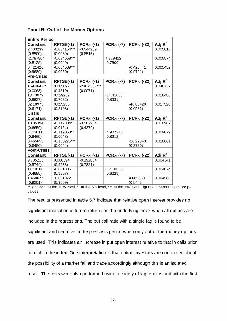
279


Entire Period


2.403239 (0.8500)

-0.084154*** (0.0069)

-3.544969 (0.8515)

0.005616

-2.787804 (0.8138)

-0.084658*** (0.0049)

4.929412 (0.7800)

0.005574

0.421426 (0.9689)

-0.084539*** (0.0050)

-0.426441 (0.9791)

0.005452

Pre-Crisis


169.4642** (0.0068)

0.085092 (0.4519)

-230.4337*** (0.0071)

0.046732

13.43079 (0.8627)

0.029259 (0.7032)

-14.41068 (0.8931)

0.018486

32.18975 (0.6171)

0.025233 (0.8193)

-40.83420 (0.6586)

0.017528

Crisis


10.05394 (0.6659)

-0.112334** (0.0124)

-32.02954 (0.4279)

0.010967

-4.036116 (0.8469)

-0.119068** (0.0048)

-4.907345 (0.8912)

0.009079

8.465655 (0.6486)

-0.120275*** (0.0044)

-28.27943 (0.3730)

0.010661

Post-Crisis


9.705213 (0.5744)

0.000394 (0.9933)

-9.192034 (0.7321)

0.004341

11.49106 (0.4659)

-0.001835 (0.9697)

-12.18855 (0.6229)

0.004074

1.450677 (0.9201)

-0.001972 (0.9669)

4.609853 (0.8448

0.004588


The results presented in table 5.7 indicate that relative open interest provides no

significant indication of future returns on the underlying index when all options are

included in the regressions. The put call ratio with a single lag is found to be

significant and negative in the pre-crisis period when only out-of-the-money options

are used. This indicates an increase in put open interest relative to that in calls prior

to a fall in the index. One interpretation is that option investors are concerned about

the possibility of a market fall and trade accordingly although this is an isolated

result. The tests were also performed using a variety of lag lengths and with the first-

280

difference of the open interest ratio as the informational dependent variable. The

results were not sensitive to these adjustments.

Table 5.8 Returns on Portfolio of Individual Financial Stocks and FTSE100

Index Option Trading Volume

The regression in equation (5.3) is run again with the return on the financial stock

portfolio replacing the FTSE100 as the dependent variable.


Entire Period

Constant RPort(-1) PCRTV (-1) PCRTV (-7) PCRTV (-22) Adj R2

-0.002803 (0.5134)

0.012219 (0.7880)

0.004145 (0.5508)

0.000454

0.001121 (0.7675)

0.009147 (0.8314)

-0.002752 (0.6546)

0.000249

-0.000566 (0.8871)

0.009030 (0.8339)

0.000166 (0.9798)

0.000082

Pre-Crisis


-0.005656 (0.2905)

0.084961 (0.4468)

0.009714 (0.2378)

0.015336

0.003550 (0.5650)

0.045853 (0.6654)

-0.005310 (0.5868)

0.006726

-0.007350 (0.1638)

0.024780 (0.7950)

0.012465 (0.1176)

0.022298

Crisis


-0.005130 (0.4776)

-0.005261 (0.9207)

0.004686 (0.7116)

0.000433

0.000937 (0.8898)

-0.10400 (0.8347)

-0.006026 (0.6025)

0.000680

-0.011065 (0.1030)

-0.008355 (0.8641)

0.015062 (0.1847)

0.003790

Post-Crisis


0.001576 (0.8485)

0.025812 (0.7502)

-0.002117 (0.8780)

0.000801

0.002281 (0.7261)

0.027680 (0.7143)

-0.003445 (0.7544)

0.000920

0.005981 (0.4329)

0.028031 (0.7108)

-0.010323 (0.4458)

0.002414

281

Panel B: Out-of-the-Money

Entire Period


0.000901 (0.8243)

0.020406 (0.6418)

-0.002074 (0.7486)

0.001143

0.000631 (0.8635)

0.020373 (0.6427)

-0.00164 (0.7748)

0.001189

-0.0017 (0.5874)

0.020729 (0.6360)

0.002295 (0.6489)

0.001139

Pre-Crisis


-0.007910 (0.0985)

0.062860 (0.5693)

0.012449* (0.0649)

0.011978

0.001559 (0.7743)

0.053211 (0.6322)

-0.002403 (0.7658)

0.015334

0.006365* (0.0763)

0.055558 (0.5942)

-0.009957 (0.1102)

0.000124

Crisis


0.004526 (0.4751)

0.005879 (0.9090)

-0.012098 (0.2979)

0.003017

-0.004677 (0.5021)

0.004018 (0.9391)

0.004324 (0.7159)

0.005189

-0.010672* (0.0744)

0.003224 (0.9498)

0.003224 (0.9498)

0.014886 (0.1629)

0.001696

Post-Crisis


0.003672 (0.6463)

0.035351 (0.6487)

-0.005757 (0.6559)

0.002201

0.005604 (0.3953)

0.032221 (0.6799)

-0.009208 (0.3882)

0.001087

0.002801 (0.6045)

0.035213 (0.6410)

-0.004223 (0.6468)

0.002522


Only one of the coefficients in Table 5.8, the put to call ratio with one lag, is found to

be statistically significant. Even then the relationship is very weak. Hence it is not

possible to infer any return predictability from FTSE100 index trading volume on the

portfolio of financial stocks in the crisis period or sub-periods.

282

Table 5.9 Returns on Portfolio of Individual Financial Stocks and FTSE100

Index Option Open Interest


Entire Period

Constant RPort(-1) PCROI(-1) PCROI (-7) PCROI (-22) Adj R2

0.001860 (0.6659)

0.009211 (0.8308)

-0.004280 (0.5591)

0.000226

0.005357 (0.1704)

0.009069 (0.8332)

-0.010788 (0.1030)

0.000998

0.003256 (0.4550)

0.009036 (0.8343)

-0.006910 (0.3555)

0.000459

Pre-Crisis


-0.030514 (0.5887)

0.058508 (0.5667)

0.053690 (0.5840)

0.00503

0.074945 (0.2092)

0.050679 (0.6088)

-0.131220 (0.2131)

0.014126

0.107107 (0.2347)

0.040481 (0.6480)

-0.188017 (0.2382)

0.020263

Crisis


-0.024111 (0.5587)

-0.011055 (0.8276)

0.039286 (0.5921)

0.001097

0.005874 (0.8878)

-0.009759 (0.8453)

-0.015172 (0.8378)

0.000245

-0.010008 (0.8040)

-0.009839 (0.8444)

0.013570 (0.8497)

0.000193

Post-Crisis


0.002506 (0.5443)

0.027470 (0.7185)

-0.004161 (0.6048)

0.000925

0.006584 (0.0854)

0.028419 (0.7084)

-0.012320 (0.1038)

0.002398

0.004118 (0.3944)

0.027044 (0.7233)

-0.007383 (0.4183)

0.001256

283


Entire Period


-0.000906 (0.8604)

0.020049 (0.6408)

0.020049 (0.6404)

0.001234

-0.001284 (0.7977)

0.020396 (0.6381)

0.001565 (0.8311)

0.001182

-0.005158 (0.3530)

0.018520 (0.6599)

0.007868 (0.3399)

0.000709

Pre-Crisis


0.028208** (0.0464)

0.102423 (0.3163)

-0.039057** (0.0419)

0.01753

-0.006039 (0.7485)

0.069482 (0.5674)

0.008437 (0.7454)

0.014734

0.008389 (0.6266)

0.054235 (0.5999)

-0.011765 (0.6371)

0.013999

Crisis


-0.000235 (0.9696)

0.005311 (0.9179)

-0.003764 0.005239

-0.002631 (0.6760)

0.004939 (0.9238)

0.000702 (0.9453)

0.005506

-0.007007 (0.3875)

0.004218 (0.9352)

0.008435 (0.5094)

0.004277

Post-Crisis


0.001223 (0.9041)

0.036081 (0.6340)

-0.001290 (0.9339)

0.002917

0.002199 (0.8137)

0.036183 (0.6375)

-0.003046 (0.8312)

0.002681

-0.004728 (0.5909)

0.033361 (0.6376)

0.009168 (0.5055)

0.000435


None of the coefficients in the results presented in Table 5.9, Panel A are statistically

significant. In Panel B the coefficient for 1 lag of the put to call open interest ratio is

significant and negative for the pre-crisis period. This can be interpreted as limited

evidence of return predictability in financial stocks from index option open interest

prior to the crisis period. However, in aggregate the hypothesis that daily lagged

relative trading volume and open interest from equity options has no explanatory

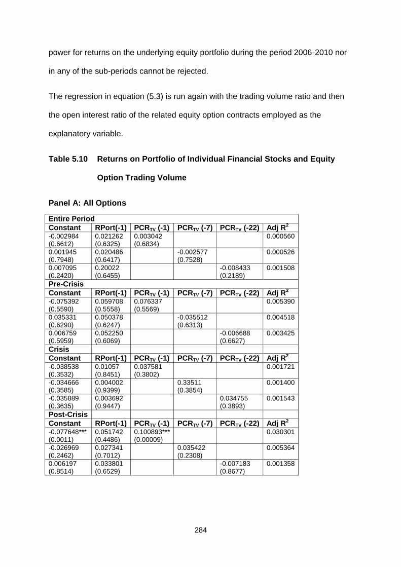
284

power for returns on the underlying equity portfolio during the period 2006-2010 nor

in any of the sub-periods cannot be rejected.

The regression in equation (5.3) is run again with the trading volume ratio and then

the open interest ratio of the related equity option contracts employed as the

explanatory variable.

Table 5.10 Returns on Portfolio of Individual Financial Stocks and Equity

Option Trading Volume


Entire Period


-0.002984 (0.6612)

0.021262 (0.6325)

0.003042 (0.6834)

0.000560

0.001945 (0.7948)

0.020486 (0.6417)

-0.002577 (0.7528)

0.000526

0.007095 (0.2420)

0.20022 (0.6455)

-0.008433 (0.2189)

0.001508

Pre-Crisis


-0.075392 (0.5590)

0.059708 (0.5558)

0.076337 (0.5569)

0.005390

0.035331 (0.6290)

0.050378 (0.6247)

-0.035512 (0.6313)

0.004518

0.006759 (0.5959)

0.052250 (0.6069)

-0.006688 (0.6627)

0.003425

Crisis


-0.038538 (0.3532)

0.01057 (0.8451)

0.037581 (0.3802)

0.001721

-0.034666 (0.3585)

0.004002 (0.9399)

0.33511 (0.3854)

0.001400

-0.035889 (0.3635)

0.003692 (0.9447)

0.034755 (0.3893)

0.001543

Post-Crisis


-0.077648*** (0.0011)

0.051742 (0.4486)

0.100893*** (0.00009)

0.030301

-0.026969 (0.2462)

0.027341 (0.7012)

0.035422 (0.2308)

0.005364

0.006197 (0.8514)

0.033801 (0.6529)

-0.007183 (0.8677)

0.001358

285


Entire Period


0.001249 (0.5915)

0.018092 (0.6797)

-0.002942 (0.4391)

0.000738

0.000937 (0.7064)

0.020380 (0.6441)

-0.002386 (0.5852)

0.000917

0.000458 (0.8261)

0.020382 (0.6435)

0.001542 (0.6576)

0.001138

Pre-Crisis


0.000920 (0.7378)

0.062028 (0.5511)

-0.001727 (0.7090)

0.014845

0.000447 (0.8225)

0.056973 (0.5919)

-0.000808 (0.8290)

0.015953

-0.004166 (0.1051)

0.044609 (0.6121)

0.008116* (0.0501)

0.010774

Crisis


0.004833 (0.3405)

-0.006921 (0.8896)

-0.013144 (0.1052)

0.001223

0.001282 (0.7750)

0.004076 (0.9372)

-0.006509 (0.4085)

0.003820

0.006013 (0.1858)

-0.002222 (0.9650)

-0.015127* (0.0515)

0.003213

Post-Crisis


-0.002043 (0.6806)

0.038935 (0.6053)

0.004567 (0.5670)

0.002025

0.001096 (0.8497)

0.036539 (0.6268)

-0.001219 (0.9003)

0.002857

-0.002939 (0.4912)

0.035104 (0.6368)

0.006294 (0.3496)

0.001117


The results presented in Table 5.10 are mostly insignificant. In Panel A, only relative

trading volume lagged by one day during the crisis period is statistically significant

and even in this case the value of the R-squared statistic is very low. In Panel B, the

put to call ratio with 22 lags is significant with 22 lags. The relationship is positive in

the pre-crisis period and negative in the crisis period suggesting that little can be

inferred in terms of predictability. The tests were also run with 2 and 3 lags but no

statistically significant coefficients were produced. Furthermore, the results are

286

insensitive to using the first-difference of the trading volume or open interest ratio as

the informational explanatory variable. A statistically significant but small relationship

is found when contemporaneous trading volume is used.

Table 5.11 Returns on Portfolio of Individual Financial Stocks and Equity

Option Open Interest


Entire Period

Constant RPort(-1) PCROI (-1) PCROI (-7) PCROI (-22) Adj R2

0.003678 (0.1681)

0.018619 (0.5197)

-0.00571 (0.1209)

0.002428

0.002949 (0.2716)

0.019079 (0.5106)

-0.004570 (0.2050)

0.01773

0.005319** (0.0497)

0.017168 (0.5559)

-0.007886** (0.0301)

0.004417

Pre-Crisis


0.032900 (0.1101)

0.058180 (0.5552)

-0.033080 (0.1122)

0.027548

-0.001215 (0.8780)

0.053339 (0.5930)

0.001502 (0.8543)

0.003158

0.001447 (0.7789)

0.052566 (0.5984)

-0.00134 (0.8099)

0.003397

Crisis


-0.003906 (0.9142)

0.006549 (0.8984)

0.001504 (0.9680)

0.000049

-0.049006 (0.2373)

0.003943 (0.9403)

0.048617 (0.2613)

0.003539

-0.006173 (0.8590)

0.006396 (0.9028)

0.003868 (0.9137)

0.000068

Post-Crisis


-0.053959** (0.0321)

0.029801 (0.6857)

0.098710** (0.0270)

0.006325

-0.013653* (0.0905)

0.031217 (0.6764)

0.025504* (0.0657)

0.003282

0.016746 (0.4491)

0.028835 (0.6378)

-0.028426 (0.4769)

0.008395

287


Entire Period


-0.003711 (0.3284)

0.025302 (0.5514)

0.007302 (0.4167)

0.000280

-0.002147 (0.5645)

0.01981 (0.6584)

0.00391 (0.6566)

-0.002103 (0.5713)

0.020281 (0.6490)

0.00376 (0.6654)

0.000871

Pre-Crisis


-0.017441 (0.0648)

0.10838 (0.3046)

0.040387* (0.0679)

0.017458

0.006646 (0.5349)

0.060529) (0.5715)

-0.015398 (0.5370)

0.010266

0.002442 (0.7105)

0.058754 (0.5726)

-0.005715 (0.7017)

0.015227

Crisis


-0.019391*** (0.0056)

0.016374 (0.7441)

0.034714** (0.0169)

0.014421

-0.010663 (0.1430)

-0.00235 (0.9658)

0.017171 (0.2398)

0.000945

-0.011704 (0.1682)

-0.000732 (0.9891)

0.019866 (0.2372)

0.000732

Post-Crisis


0.000530 (0.9396)

0.036169 (0.6074)

-0.000178 (0.9908)

0.002921

-0.001339 (0.8409)

0.036058 (0.6386)

0.003435 (0.8160)

0.002606

-0.00008 (0.9891)

0.036344 (0.6310)

0.000994 (0.9399)

0.002893


The results in Table 5.11 show few significant coefficients; four in total, evenly split

between Panels A and B and with no consistency in time. Once again there is little

evidence of return predictability for the equity portfolio provided by equity option

open interest.

The results presented in the preceding tables provide a clear rejection of the

hypothesis that relative trading volume and open interest provide information on spot

market returns when daily data is analysed. Nevertheless the results provide some

support to the argument of Pan and Poteshman (2006) that trading volume and open

288

interest data for out-of-the-money options contain more information than is contained

in the trading volume and open interest data in aggregate. Consequently it cannot be

inferred that any trading information can be gathered by analysing lagged trading

volume or lagged open interest that will be useful in achieving abnormal returns.

These results are insensitive to the selection of sample period across the duration of

the recent financial crisis and are consistent with the efficient markets hypothesis.

Modelling the Contemporaneous Relationship between Equity Returns,

Trading Volume and Open Interest

The results presented in Tables 5.12 to 5.15 are produced by running the

regressions given in equations (5.5) and (5.6). The contemporaneous relationship

between returns on the financial portfolio and corresponding trading volume and

open interest ratios is examined, with no initial assumption regarding the direction.

The hypothesis to be tested is that there is a price discovery relationship between

returns on the portfolio of financial stocks and the trading volume and open interest

of options written on those stocks.

289

Table 5.12 Returns on Financial Portfolio and Trading Volume

Dependant variable is the portfolio return:


Entire Period

Constant RPort(-1) PCRTV Adj R2

0.015463* (0.0652)

0.017146 (0.7058)

-0.017146* (0.0506)

0.005439

Pre-Crisis


0.175229 (0.3906)

0.035016 (0.7546)

-0.176656 (0.3904)

0.016491

Crisis


0.077003 (0.1012)

0.007166 (0.8896)

-0.082776* (0.0873)

0.008229

Post-Crisis


0.051677 (0.1064)

0.028515 (0.7151)

-0.065957 (0.1021)

0.013255


Entire Period


0.006464*** (0.0010)

0.018634 (0.6717)

-0.012766*** (0.0001)

0.008670

Pre-Crisis


-0.001835 (0.4525)

0.065775 (0.5345)

0.003604 (0.3446)

0.010280

Crisis


0.009911** (0.0344)

-0.007281 (0.8906)

-0.022559*** (0.0034)

0.014743

Post-Crisis


0.008109** (0.0331)

0.041064 (0.5853)

-0.014097 (0.0186)

0.005655


In Panel A, the signs attached to the trading volume ratio are all negative indicating

the expected result that negative returns on the equity portfolio are linked

contemporaneously with increases in the trading volume ratio. However the

relationship is only statistically significant over the entire period and the crisis period

290

with the associated R-squared statistics weak in each case. In Panel B the

relationship is the same but significant at the 1% level. This result suggests the

possibility of a weak price discovery relationship particularly when the trading volume

of out-of-the-money put options is examined.

Table 5.13 Returns on Financial Portfolio and Trading Volume

Dependant Variable is the Trading Volume Ratio.


Entire Period

Constant RPort RPort(-1) R2

0.879722*** (0.0000)

-0.282891* (0.0520)

0.005108

0.879701*** (0.0000)

-0.1811538 (0.1391)

0.002104

Pre-Crisis


0.990634*** (0.0000)

-0.082829 (0.3823)

0.015296

0.990633 (0.0000)

-0.102895* (0.0875)

0.023551

Crisis


0.959796 (0.1024)

-0.098825 (0.1024)

0.008177

0.960054*** (0.0000)

0.005102 (0.9189)

0.000022

Post-Crisis


0.774928 (0.0000)

-0.186464 (0.1010)

0.012444

0.774865*** (0.0000)

-0.076132 (0.3350)

0.002074

291


Entire Period


0.530527*** (0.0000)

-0.778918*** (0.0009)

0.009973

0.530714*** (0.0000)

-0.136211 (0.5154)

0.000305

Pre-Crisis


0.515786*** (0.0000)

1.520053 (0.3851)

0.005120

0.516014*** (0.0000)

-1.652115 (0.3857)

0.005930

Crisis


0.538278*** (0.0000)

-0.895759** (0.0156)

0.020119

0.539076*** (0.0000)

-0.542153* (0.0676)

0.004629

Post-Crisis


0.544532*** (0.0000)

-0.593570** (0.0472)

0.008177

0.544113*** (0.0000)

0.336914 (0.2118)

0.000522


The results in Panel A indicate that, over the entire period there is a significant

negative impact of equity portfolio return on the trading volume ratio. There is also a

significant negative impact of lagged portfolio return during the pre-crisis period. The

signs on all but the lagged portfolio in the crisis period are negative as expected. In

Panel B there is a significant and negative impact of equity portfolio return on the

trading volume ratio in all but the pre-crisis period. This relationship extends to the

lagged return on the equity portfolio over the crisis period. It seems just as likely that

trading volume reacts to stock returns rather than price discovery information flowing

in the opposite direction.

292

Table 5.14 Returns on Financial Portfolio and Open Interest

Dependant variable is the portfolio return:


Entire Period

Constant RPort(-1) PCROI Adj R2

0.003100 (0.2381)

0.018829 (0.6719)

-0.004764 (0.1662)

0.001887

Pre-Crisis


-0.190039 (0.2591)

0.048439 (0.6115)

-0.191775 (0.2573)

0.016426

Crisis


-0.087581** (0.0260)

-0.004900 (0.9263)

-0.088930** (0.0281)

0.011484

Post-Crisis


-0.345265* (0.0625)

0.017917 (0.7835)

-0.627054* (0.0608)

0.018125


Entire Period


0.010361*** (0.0084)

0.005688 (0.8869)

-0.022902** (0,0145)

0.013903

Pre-Crisis


0.024201* (0.0761)

-0.011383 (0.9128)

-0.055869 (0.0928)

0.047215

Crisis


0.007820 (0.2801)

-0.000471 (0.9930)

-0.020356 (0.1873)

0.001406

Post-Crisis


0.016397** ((0.0314)

0.011087 (0.8625)

-0.030961* (0.0624)

0.021261


The signs of the coefficients attached to the open interest ratio in each case are

negative as expected indicating that falling index returns are associated with an

increase in the number of open positions in put options on financial stocks at the

close of each trading day. The coefficients are statistically significant for the crisis

293

and post-crisis period in Panel A and the entire and post-crisis periods in Panel B.

These results provide some evidence that the relationship has changed over the

recent financial crisis. It is not possible to reject a contemporaneous impact of open

interest on the financial stock portfolio returns indicating fairly weak price discovery.

Table 5.15 Returns on Financial Portfolio and Open Interest

Dependant variable is the open interest ratio


Entire Period


0.715148*** (0.0000)

-0.317947 (0.1635)

0.001557

0.715292*** (0.0000)

-0.329773 (0.1499)

0.001676

Pre-Crisis


0.992128*** (0.0000)

0.072247 (0.1993)

0.014089

0.992140*** (0.0000)

0.024787 (0.7721)

0.001655

Crisis


0.917544*** (0.0000)

0.360913 (0.3000)

0.835438

0.917643*** (0.0000)

0.383181 (0.2751)

0.009839

Post-Crisis


0.551521*** (0.0000)

0.027947** (0.0424)

0.017808

0.551522*** (0.0000)

0.024910* (0.0686)

0.014149

294


Entire Period


0.465842*** (0.0000)

-0.676176** (0.0127)

0.015606

0.465985*** (0.000)

-0.641236 (0.0215)

0.014049

Pre-Crisis


0.432625*** (0.0000)

-1.188191* (0.0533)

0.065598

0.432727*** (0.0000)

-1.274474* (0.0507)

0.074000

Crisis


0.494558*** (0.0000)

-0.339464 (0.1597)

0.006908

0.494722*** (0.0000)

-0.266254 (0.2612)

0.004250

Post-Crisis


0.515435*** (0.0000)

-0.807342* (0.0565)

0.025279

0.515429*** (0.0000)

-0.814805* (0.0623)

0.025757


In Panel A, although for the entire period the signs on the coefficients attached to the

dependent variables are negative they are positive for each sub-period. However the

coefficients for all periods other than the post-crisis are not statistically significant.

Hence it is not possible to infer any consistent relationship between

contemporaneous and lagged stock returns and open interest using the aggregate

open interest of the equity options. In Panel B, the coefficients attached to portfolio

returns in the entire, pre-crisis and post-crises periods are negative and significant. It

follows that, when only out-of-the-money options are examined, there is evidence

that trading volume and open interest react to returns on the underlying assets.

295

5.6 A Behavioural Perspective on Trading Volume and Open Interest

In this section it is hypothesised that trading behaviour in the UK market occurs as a

rational response to spot market activity as traders update their beliefs regarding risk

in accordance with the direction and magnitude of market returns. If this is the case

then total trading volume should increase (decrease) with negative (positive) returns

that are contemporaneous or lagged by one day. It is unlikely that lagged returns of

more than one day will have a significant effect on trading volume. However, from a

behavioural perspective a series of returns of the same sign may lead conservative

traders to perceive this to be a trend and to update their beliefs accordingly. A

consequence would be that a series of negative returns would lead to an increase in

put purchases relative to calls and vice versa. Table 5.16 presents the results from

running equation (5.7) where the index option trading volume ratio is regressed on

the FTSE100 returns and a dummy variable. The dummy variable is equal to 1 if

three or more of the consecutive preceding FTSE100 returns are of the same sign

and zero otherwise. Tests are run for the entire period only, as the clustering of runs

of positive and negative returns is likely to bias the results for sub-periods.

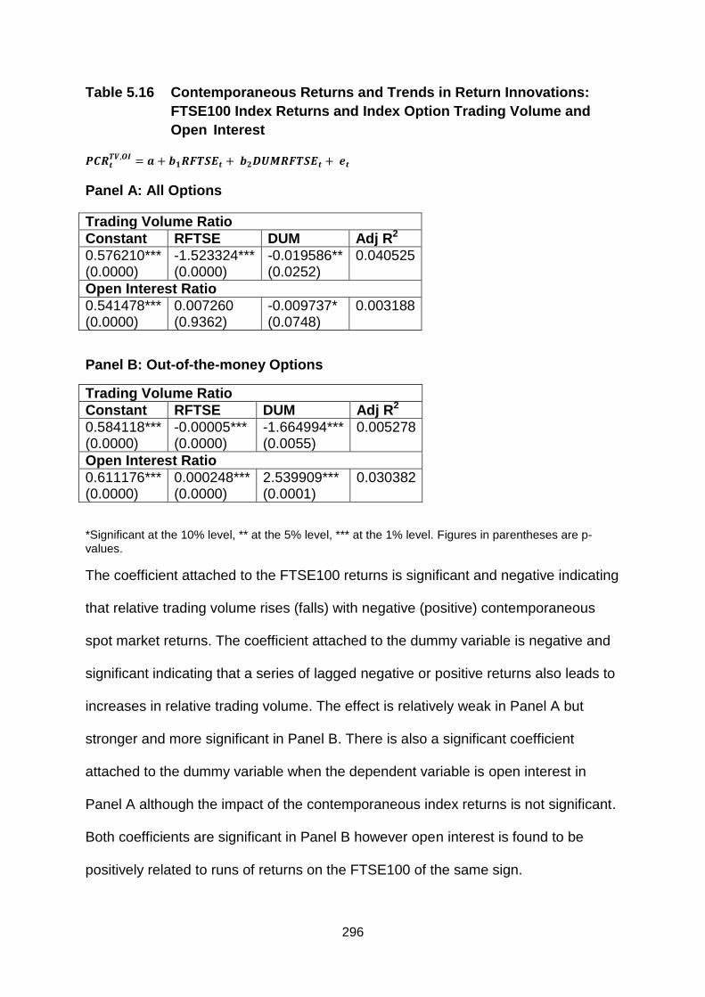
296

Table 5.16 Contemporaneous Returns and Trends in Return Innovations:

FTSE100 Index Returns and Index Option Trading Volume and

Open Interest


Trading Volume Ratio

Constant RFTSE DUM Adj R2

0.576210*** (0.0000)

-1.523324*** (0.0000)

-0.019586** (0.0252)

0.040525

Open Interest Ratio

0.541478*** (0.0000)

0.007260 (0.9362)

-0.009737* (0.0748)

0.003188

Panel B: Out-of-the-money Options

Trading Volume Ratio

Constant RFTSE DUM Adj R2

0.584118*** (0.0000)

-0.00005*** (0.0000)

-1.664994*** (0.0055)

0.005278

Open Interest Ratio

0.611176*** (0.0000)

0.000248*** (0.0000)

2.539909*** (0.0001)

0.030382


The coefficient attached to the FTSE100 returns is significant and negative indicating

that relative trading volume rises (falls) with negative (positive) contemporaneous

spot market returns. The coefficient attached to the dummy variable is negative and

significant indicating that a series of lagged negative or positive returns also leads to

increases in relative trading volume. The effect is relatively weak in Panel A but

stronger and more significant in Panel B. There is also a significant coefficient

attached to the dummy variable when the dependent variable is open interest in

Panel A although the impact of the contemporaneous index returns is not significant.

Both coefficients are significant in Panel B however open interest is found to be

positively related to runs of returns on the FTSE100 of the same sign.

297

The observation that the results are strongest in Panel B can be interpreted as

options investors turning to out-of-the-money options following an upward or

downward trend. The negative coefficient attached to the dummy variable regressed

on the trading volume ratio can be interpreted as investors trading more put (call)

options than call (put) options following a consecutive 3-day negative (positive) run.

The positive coefficient attached to the dummy variable regressed on the open

interest ratio is more difficult to rationalise. The implication is that more put (call)

positions are closed out relative to call (put) positions in a falling (rising) market. As

the options are European-style no early exercise can take place. It follows that a

change in the open interest ratio is as a result of options being either written or

closed out by taking offsetting positions. Another point to note is that open interest

will contain option positions that remain open for a period of time but have no trading

volume. A run of stock market rises (falls) results in more calls (puts) ceasing to be

out-of-the-money. This means that they exit the out-of-the-money data set whilst the

corresponding, previously in-the-money options of the other category enter. Should

there be a sharp rise or fall in the underlying market, this will result in a considerable

impact on the size of the open interest ratio.

A further test is performed to establish the impact of returns on the portfolio of

financial stocks on the trading volume and open interest ratios with results presented

in Table 5.17.

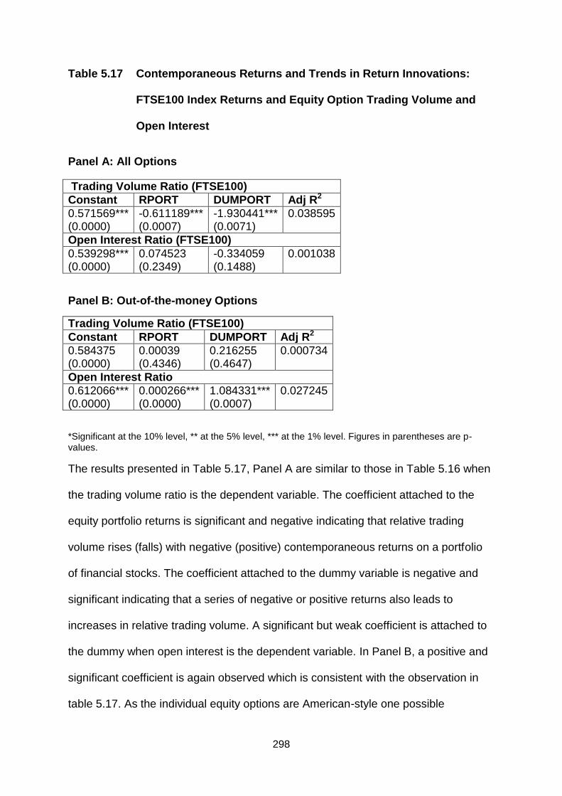
298


FTSE100 Index Returns and Equity Option Trading Volume and

Open Interest


Trading Volume Ratio (FTSE100)

Constant RPORT DUMPORT Adj R2

0.571569*** (0.0000)

-0.611189*** (0.0007)

-1.930441*** (0.0071)

0.038595

Open Interest Ratio (FTSE100)

0.539298*** (0.0000)

0.074523 (0.2349)

-0.334059 (0.1488)

0.001038


Trading Volume Ratio (FTSE100)


0.584375 (0.0000)

0.00039 (0.4346)

0.216255 (0.4647)

0.000734

Open Interest Ratio

0.612066*** (0.0000)

0.000266*** (0.0000)

1.084331*** (0.0007)

0.027245


The results presented in Table 5.17, Panel A are similar to those in Table 5.16 when

the trading volume ratio is the dependent variable. The coefficient attached to the

equity portfolio returns is significant and negative indicating that relative trading

volume rises (falls) with negative (positive) contemporaneous returns on a portfolio

of financial stocks. The coefficient attached to the dummy variable is negative and

significant indicating that a series of negative or positive returns also leads to

increases in relative trading volume. A significant but weak coefficient is attached to

the dummy when open interest is the dependent variable. In Panel B, a positive and

significant coefficient is again observed which is consistent with the observation in

table 5.17. As the individual equity options are American-style one possible

299

interpretation is that option traders display a disposition effect. This implies that the

holders of options realise gains by early exercising options that move into (or deeper

into) the money following a series of consecutive price changes in the underlying

asset. This explanation is consistent with options being held for speculative rather

than hedging purposes. However, the explanation offered is impossible to support

without precise information on the type of trades that take place on each trading day.

To complete this section of the analysis the trading volume and open interest ratios

of the equity portfolio will be regressed on the contemporaneous equity portfolio

returns and a dummy variable for the equity portfolio which is constructed in the

same way as that for the FTSE100.


Equity Portfolio Returns and Equity Option Trading Volume and

Open Interest

Trading Volume Ratio (Equity Port)


0.954329*** (0.0000)

-0.027861 (0.8885)

-1.485778*** (0.0002)

0.028537

Open Interest Ratio (Equity Port)

0.776168*** (0.0000)

-0.055089 (0.9493)

-3.263313** (0.0327)

0.010036


Trading Volume Ratio (Equity Port)


0.530322*** (0.0000)

0.000048 (0.5248)

0.166560 (0.7066)

0.001227

Open Interest Ratio

0.464168*** (0.0000)

-0.000131** (0.0104)

-1.820266*** (0.0000)

0.032729


300

The results in Table 5.18, Panel A indicate no significant relationship between

contemporaneous equity portfolio returns and the respective trading volume and

open interest ratios. There is however a significant negative relationship between the

dummy variable and each dependent variable. This result indicates that a run of

positive (negative) returns of the same sign is associated with a decrease (increase)

in relative trading volume and open interest. In Panel B, both coefficients are

insignificant for the trading volume ratio. Interestingly, the coefficient attached to the

dummy variable for equity portfolio returns is negative in contrast to that in Tables

5.17 and 5.18. This does however support the hypothesis that open interest of puts

rises relative to that of calls following a run of consecutive daily stock returns of the

same sign.

The findings in this section are consistent with the behavioural models of Barberis,

Shleifer and Vishny (1998) in the equity market and Poteshman (2001) in the options

market which were discussed in detail in Chapter 2. Options market traders seem to

display conservatism in their trading behaviour in response to returns in the

aggregate and individual equity markets. Conversely, when these returns follow a

consecutive series of innovations of the same sign, investors demonstrate

representativeness by perceiving this as a trend and modify their trading behaviour

accordingly.

301

5.7 Conclusion

The results presented above clearly indicate that there is no evidence of stock

market predictability in daily trading volume and open interest data from the UK

exchange-traded options market. This implies that published options market

information cannot be used by investors to construct profitable trading strategies.

This does not necessarily imply that particular categories of trader are not privy to

private information, as the Euronext LIFFE data cannot be disaggregated for the

purposes of such an examination. The rejection of predictability may not be

interpreted as an automatic rejection of a price discovery function. Price discovery

will be a consequence of the trades of sophisticated investors with access to private

information. These findings are consistent with market efficiency as there appear to

be no exploitable opportunities from predictability and a simultaneous contribution to

informational efficiency through the price discovery function.

A key indication of the behavioural traits evident in equity markets is identified in the

analysis of the response of relative trading volume to a consecutive series of returns

of the same sign. The relationship is consistent across index and equity options

whether in aggregate or restricted to out-of-the-money contracts. The evidence

presented is consistent with investors‟ conservative responses to individual pieces of

information and updates to beliefs when information follows a quantity of similar

information. The updating occurs when the information is perceived to be

representative of a trend. The results are a little less clear for out-of-the-money

options when open interest is the dependent variable. Behavioural explanations have

been offered for the results however the composition of the dataset is likely to be

altered following consecutive rises or falls in the underlying asset particularly if there

are a large number of options which are fairly close-to-the-money. In interesting

302

extension to this work would be to further segregate the trading volume and open

interest data according to moneyness; particularly options that are fairly deep in- or

out-of-the-money.

A limitation of this study arises because the Euronext LIFFE database does not sub-

divide trading volume by opening or closing of positions or by the category of

investor carrying out the transaction. An obvious extension to this work would be to

perform analysis of the UK market using data which can be sub-divided in terms of

trader sophistication and type of transaction. If trading is correlated with private

information then transactions data from the UK options market is likely to provide

valuable insights into option trader behaviour and possible predictions for future

stock price movements.

303

Chapter 6

On the Presence of Momentum Effects

and Short-Term Overreaction in the UK

FTSE100 Index Options Market 2006-

2010

304

6.1 Introduction

The overall objective of this chapter is to test for evidence of momentum effects and

short-term overreaction in the UK FTSE100 index options market. More precisely,

the relationship between option prices and past market moves and the relationship

between option implied volatility and ex post realised volatility will be examined.

Again the focus will be on the financial crisis period of 2007/8 although momentum

and overreaction will also be evaluated across the pre- and post-crisis periods. The

first hypothesis is that momentum in stock prices will contribute to investors‟

expectations about future stock prices. These investor expectations will, in turn,

affect the demand for and supply of call and put options. If, as a consequence, the

forces of demand and supply induce price pressure then investor expectations about

future stock prices provides an additional parameter for the pricing of options. The

second hypothesis is that options market investors exhibit short-term overreaction to

price changes. However, in common with Gettleman, Julio and Risik (2011) it is

hypothesised that overreaction is conditional on significant price changes over a

relatively short time period.

Literature which evaluates underreaction and momentum strategies in the context of

equity markets is relatively common and has been discussed in Chapter 1, section

1.7.2. Evidence of the relationship between option prices and stock market

momentum is relatively sparse in comparison. However Amin, Coval and Seyhun

(2004) partially address this apparent gap in the literature and produce evidence to

indicate that, where markets are imperfect, past stock returns exert a strong

influence on S&P100 option prices.

305

Evidence of long term overreaction in the options market was first presented by Stein

(1989). Poteshman advanced research into this area and produced evidence

consistent with long term overreaction and short term underreaction. In contrast to

Poteshman, evidence of short term overrreaction conditional on preceding sharp

stock price moves was identified by Gettleman, Julio and Risik (2011). Gettleman et

al then constructed portfolios of stocks and options, on the basis of this overreaction,

that were found to produce consistent abnormal profits. All of the above studies

focus on the US aggregate or individual stock and options markets.

This chapter contributes to the literature by analysing the UK index options market

for both evidence of momentum effects and conditional short term overreaction. If

evidence of these effects are found in options markets, these findings will

complement similar evidence found in equity markets most notably be DeBondt and

Thaler (1985, 1987) and Jegadeesh and Titman (1993). Consistent with chapters 4

and 5, the analysis centres on the time period around the 2007/8 financial crisis.

The motivation to examine for a momentum effect in the UK market is to identify

whether a demand-driven parameter is important in the pricing of FTSE100 index

options. Tests for momentum effects involve a non-parametric approach of put-call

parity violations and a parametric approach of implied volatility spreads. The

behaviour of each of these measures is examined in light of previous returns on the

underlying market. The financial crisis of 2007/8 should be a particularly interesting

time to examine put-call parity violations as it contains a period of restrictions on

short selling. Nishiotis and Rompolis (2010) find a significant increase in the

magnitude of put-call parity violations during the 2008 short sales ban in the US.

They attribute the increase in the size of violations to either overpriced stocks during

the ban as a consequence of the limited ability of arbitrageurs to offset the influence

306

of overly optimistic investors on stock prices, or the delay in informational feedback

from the options market to the stock market. They also find that put prices become

expensive relevant to equivalent calls as they provide an alternative to short selling.

Furthermore the magnitude of put-call parity violations are found to be significant

predictors of future stock market returns.

The second objective of this chapter is to test for short-term option trader

overreaction to sharp declines in stock prices. Anecdotal evidence that investors

access the options market to act rapidly on pressing information, as noted in

Gettleman et al, partly motivates an evaluation of overreaction. Furthermore,

evidence of systematic short-term overreaction to declines in stock price may offer

opportunities for profitable trading strategies which poses a challenge to the efficient

markets hypothesis.

6.2 Data

The data set comprises European style put and call options written on the FTSE100

index. Restricting the sample to the largest and most actively traded segment of the

UK traded options market reduces the possibility of any liquidity issues. Options data

are purchased from Euronext LIFFE whilst data on interest rates and Futures prices

are obtained from Datastream. The option prices are daily closing prices and are

calculated as the mid-point of the bid-offer spread. The spot price is that of the

FTSE100 index, taken when the options market closes, for the put-call parity tests

and the relevant futures price for the implied volatility spreads.

The entire sample period runs from 8th September 2006 to 31st December 2010

although various sub-periods are selected in the analysis. Omissions in the LIFFE

database have led to the exclusion of 37 days of observations from the sample.

307

Options without positive trading volume are also excluded. All but four of these

omitted observations are from 2010. The sample contains 18,020 matched pairs of

options.25 Options are „paired‟ by either strike price or moneyness depending upon

the type of test to be performed. Options need to be paired by strike price for the put-

call boundary violation tests and by moneyness for the implied volatility spread.

6.3 Momentum

6.3.1 Methodology

The hypothesis to be tested is that there is a divergence of put and call prices as a

function of past stock returns over the period September 2006 through December

2010. An increase in stock prices over a 60-day period will lead to an increase in the

price of calls relative to that of puts and a corresponding decrease will lead to an

increase in the price of puts relative to that of calls. The 60-day period is consistent

with that selected by Amin, Coval and Seyhun (2004) and, although not definitive, is

judged a reasonable time frame for momentum tests and is sufficiently distinct from

the 5-day event period used in the subsequent overreaction tests. The options data

comprises end of day prices, strike prices and maturities for calls and puts. Options

are sorted into pairs in terms of moneyness and maturity. For example, for the put-

call-parity tests, a nearest to the money series is produced containing put and call

options with identical specifications. Four further series are produced: an in (out)-of

the money put (call) with the corresponding (out-of) in-the-money call (put). Options

further in- or out-of-the-money are not used due to relatively low trading volume and

the consequent potential for stale prices. In terms of maturity, the options selected

25

A small number of pairs were omitted from the implied volatility spreads in cases where the software was

unable to solve the option pricing model for volatility. This also serves to exclude all pairs containing options

without a positive intrinsic value.

308

are for the first and second quoted months plus the next traded month on the March,

June, September, December cycle which has not already been included in the first

two maturity sets. Again, longer maturity options are excluded due to the problem of

stale prices. Hence the sample consists of 5 exercise prices and 3 maturity ranges

giving a total of 15 series of put-call pairs.

The underlying index value is selected at the time the options market closes. As the

options under consideration are the most liquid contracts then, consistent with

Gettleman et al, the 1 month treasury-bill rate is selected as the riskless rate of

interest. The test procedure is based on the assumption that option traders

accurately forecast future dividends up to the expiry date of each option. Stock

returns are analysed over a 60-day period.

The initial test involves identification of violations of put-call boundary conditions. In

particular the following put-call parity relationship will be examined:

(6.1)

Values of greater than zero indicate that puts are overpriced relative to calls whilst

values of less than zero indicate that calls are overpriced relative to puts.

Importantly, systematic violations of the boundary conditions as a function of past

stock returns provide evidence supportive of the market momentum hypothesis. The

probability of boundary violations is given by:

(6.2)

The use of end-of-day option prices and closing index prices comes with the caveat

that it is not possible to precisely measure deviations from put-call parity as, even in

the most liquid of markets, there are non-synchronous trading problems and

309

transactions costs. However, this does not represent a significant problem for the

momentum and overreaction tests performed here as the objective is to identify

pressures on option prices. In particular, to examine the change in magnitude of the

violations following return behaviour of the underlying index.

The second test is a parametric test of the overpricing of calls relative to puts using a

volatility spread. It is hypothesised that puts will be overpriced relative to calls

following negative 60-day returns and that calls will be overpriced relative to puts

following positive 60-day returns. Further, it is hypothesised that the more positive

(negative) the 60-day returns, the larger (smaller) will be each implied volatility

spread. The implied volatility spread is presented in equation 6.3:

(6.3)

Where C and P denote FTSE100 calls and puts and the subscripts indicate the

contracts‟ moneyness and maturity.

The LIFFE database does not contain implied volatilities hence the volatility spread

needs to be computed for each of the put-call pairs. The volatility spread is

calculated as the implied volatility of a call relative to a put with identical contract

specifications and with the same degree of moneyness. The test is model-dependent

as an option pricing model is required for the computation of implied volatility. The

Black Scholes model, with the futures price used for the underlying asset, is used to

calculate implied volatility for all of the index options. Put and call implied volatilities

as a function of positive and negative 60-day stock returns are examined separated

by exercise price and maturity. The implied volatility spreads are then regressed on

past market returns in order to quantify the differential response of put and call

implied volatilities to these returns. The regression is given in equation 6.4:

310

(6.4)

Where:

IVSM,T is the implied volatility spread for moneyness M and maturity T

RFTSEt-k,t-1 is the return on the FTSE100 index from day t-k to day t-1

6.3.2 Results

6.3.2.1 Put-Call Parity Boundary Violation Tests

The first set of results, presented in Table 6.2, report the mean boundary condition

violations and the probability of boundary condition violations (B > 0) following past

60-day returns. A negative mean violation indicates that puts are expensive relative

to equivalent calls. The results are also partitioned according to moneyness where

series 1 contains the furthest out-of (in)-the-money calls (puts), series 3 at-the-

money puts and calls and series 5 the furthest out-of(in)-the-money puts (calls).

Average moneyness (strike price divided by index) of each series is given in table

6.1.

Table 6.1 Average Moneyness of Series of Option Pairs

Series of Option Pairs

1 2 3 4 5

Moneyness 1.05805 1.02956 0.99995 0.98754 0.97913

311

Table 6.2 Put Call Parity Boundary Condition Tests Based on Past 60-Day

Market Returns

B = p – c + Se-qt – Ke-rt

Panel A

Return Mean Violation

Moneyness

1 2 3 4 5

R>0.15 -5.38865 -5.37357 -5.2451 -5.19819 -5.18209

0.15>R>0.1 -3.70799 -3.67564 -3.62176 -3.54701 -3.44933

0.1>R>0.05 -0.75972 -0.72732 -0.70061 -0.64417 -0.57583

0.05>R>0 3.990654 4.020536 4.026766 4.058361 4.113182

0>R>-0.05 1.920414 1.970254 2.000886 1.768342 1.864858

-0.05>R>-0.1 -3.27251 -3.20252 -3.18744 -2.99084 -2.92752

-0.1>R>-0.15 -2.77103 -2.66172 -2.57805 -2.33576 -7.37072

-0.15>R -3.24004 -3.16986 -3.08217 -1.71789 -3.04679

Panel B

Return Probability Violation>0

Moneyness

1 2 3 4 5

R>0.15 0.190476 0.190476 0.190476 0.190476 0.190476

0.15>R>0.1 0.257862 0.257862 0.264151 0.264151 0.264151

0.1>R>0.05 0.336296 0.334815 0.336296 0.336296 0.334815

0.05>R>0 0.467066 0.469062 0.469062 0.471058 0.467066

0>R>-0.05 0.43609 0.43609 0.438596 0.441103 0.443609

-0.05>R>-0.1 0.264798 0.264798 0.264798 0.264798 0.267913

-0.1>R>-0.15 0.326667 0.326667 0.340000 0.333333 0.313333

-0.15>R 0.296296 0.310185 0.305556 0.351852 0.347222

The mean violations for each set presented in panel A of Table 6.2 are given in index

points. The probabilities of boundary condition violations are given in panel B. An

observation is not considered a violation if its magnitude is 5 index points or less in

order to make some allowance for non-synchronous prices and trading costs.

There is a negative relationship between past index returns and the mean boundary

condition violations where past 60-day returns are either greater than 5% or less

than 5%. The relationship is increasing in returns where returns are positive

312

indicating the call prices are being bid up relative to puts by an increasing margin.

The relationship is robust to the moneyness of each series. Where past index returns

are between +5% and -5% the mean boundary violations are positive indicating that

in this region puts are overpriced relative to calls. One possible interpretation is that

positive or negative past returns of a relatively small magnitude are perceived by

investors as a downward trend. However, negative past returns of a relatively large

magnitude are perceived as temporary, indicating that investors view the market as

mean-reverting.

The probability of a boundary violation, with B > 0, is negatively related to past

returns in the range of greater than +15% to +5%. This result is inconsistent with the

market momentum hypothesis in that call prices are successively lower relative to

those of puts following increases in the value of the index. However, for the range of

returns from +5% to -0.15% the relationship is generally positive. This result is

consistent with the market momentum hypothesis in that put prices are successively

higher relative to those of calls following decreases in the value of the index. The

exception is for the range of past returns between -10% and -15% which is

associated with more positive violations than the range of past returns between -5%

and -10%. Again the relationship is robust to the moneyness of each series. The

results are quite similar to those of Amin, Cohal and Seyhun (2004), for the S&P100

market, suggesting that demand may have some role in option pricing across

markets and time periods. Amin et al interpret their findings as past returns exerting

a strong influence on index option prices. Although the results above offer some

support for this view it is debatable whether they are strong enough to draw the

same conclusion.

313

As a further robustness check the probability of positive boundary violations

conditional on a boundary violation are presented in Table 6.3. As expected this

increases the magnitude of the statistics but does not alter the results and their

interpretation. What it does indicate is that, according to the put-call parity

relationship, FTSE100 index puts are priced high relative to calls following all past

60-day returns other than those between -0.05% and +0.05%.

Table 6.3 Probability of a Put-Call Parity Violation

Return Probability Violation>0 Conditional on Probability Violation

Moneyness

1 2 3 4 5

R>0.15 0.2707 0.222222 0.222222 0.222222 0.222222

0.15>R>0.1 0.350427 0.350427 0.352941 0.358974 0.304348

0.1>R>0.05 0.466119 0.466942 0.468041 0.469979 0.42803

0.05>R>0 0.619048 0.616797 0.619236 0.620237 0.617414

0>R>-0.05 0.535385 0.537037 0.53681 0.536585 0.539634

-0.05>R>-0.1 0.326923 0.324427 0.326923 0.32567 0.311594

-0.1>R>-0.15 0.424242 0.426087 0.437768 0.434783 0.391667

-0.15>R 0.390244 0.403614 0.39521 0.444444 0.438596

6.3.2.2 Parametric Momentum Tests: Implied Volatility Spreads and Past Returns

The parametric approach permits a more general evaluation of the market

momentum hypothesis as it is not restricted to boundary violations. It also allows

analysis of the relationship between past index returns and the magnitude of

violations. Using a range of option moneyness and maturities in the sample helps to

address any systematic mispricing issues inherent in the option pricing model.

Table 6.4 contains the implied volatilities of FTSE100 put (Panel A) and call (Panel

B) options separated by moneyness and maturity. Panels A and B are sub-divided

according to positive 60-day FTSE100 returns (greater than 5%) and negative

FTSE100 returns (less than -5%).

314

Table 6.4 Put and Call Implied Volatilities Based on Past 60-Day Market

Returns

Panel A

K* 1 2 3 4 5

Call implied volatility when R > 0.05

N 0.197438 0.173219 0.173219 0.173066 0.173949

M 0.188042 0.257731 0.179455 0.177204 0.269947

F 0.193502 0.182106 0.179279 0.175032 0.170674

Call implied volatility when R < -0.05

N 0.307015 0.300577 0.293593 0.288918 0.286878

M 0.333359 0.170911 0.278298 0.288276 0.413432

F 0.390542 0.27722 0.272738 0.266802 0.260377

Panel B

K* 1 2 3 4 5

Put implied volatility when R > 0.05

N 0.094922 0.17503 0.168238 0.168577 0.166573

M 0.20351 0.282057 0.193182 0.190054 0.311298

F 0.206614 0.226741 0.218973 0.214107 0.210535

Put implied volatility when R < -0.05

N 0.138017 0.309045 0.304513 0.298316 0.292806

M 0.367267 0.204485 0.307579 0.31615 0.443885

F 0.390631 0.282212 0.323165 0.316223 0.310124

K* is the standardised exercise price which is the exercise price divided by the contemporaneous price of the underlying.

The results presented in table 6.4 are as expected in the sense that all of the implied

volatility estimates increase as the FTSE100 index declines. A switch in returns from

5% to -5% increases call implied volatility, on average, by 10.4 percentage points

315

from 19.1% to 29.5%. Similarly for puts, implied volatility increases, on average, by

10.5 percentage points from 20.2% to 30.7%. The results are mostly robust across

moneyness and maturity apart from one apparently anomalous middle maturity put-

call pair with moneyness category 2. Here the implied volatility changes are reversed

giving the appearance of a data error; however, this is not the case. To properly

assess the difference between the changes in the respective implied volatilities of

put and call options it is necessary to analyse the implied volatility spreads.

Implied volatility spreads need to be generated from put and call options which are

matched on moneyness and maturity. Achieving series that are appropriately

matched necessitates dropping some observations. Nevertheless the sample size

remains large enough (15,470 in total) to be able to draw meaningful conclusions.

Two important comparisons are made. First the difference in expensiveness

following a negative and a positive price change in the price of the underlying asset

over a 5-day period of the same magnitude. Second, the size of the volatility spread

following a 10% as opposed to a 20% change in the price of the underlying asset.

6.3.3 Implied Volatility Spread Results

Each series of implied volatility spread is categorised in terms of moneyness; series

1 is the furthest out of the money, series 3 at the money and series 5 furthest in the

money. Moneyness for calls is calculated as K/F for calls and the reciprocal for puts.

The average moneyness values for each series are presented in table 6.5. N

denotes the number of observations for each series.

316

Table 6.5 Moneyness of Implied Volatility Spreads

Maturity Near N Mid N Far N

1 1.018571 979 1.027191 1053 1.029135 1042

2 1.00917 1031 1.009484 992 1.017396 1059

3 1.000014 1055 1.000081 1042 1.000032 1060

4 0.990942 1031 0.990768 992 0.982982 1060

5 0.981802 980 0.973754 1052 0.971849 1042

Sample statistics for the at-the-money implied volatility spreads are presented in

table 6.6. These are broadly representative of the full sample. The sample statistics

for the remaining implied volatility spreads are available from the author on request.

Table 6.6 Regression of Implied Volatility Spreads on Past 60-Day Market Returns, September 1 2006 to December 31 2010

Near Mid Far

Mean -0.010144 -0.025832 -0.048980

Standard Deviation

0.045502 0.025274 0.019646

Maximum 0.196542 0.040256 0.019387

Minimum -0.136858 -0.136982 -0.128333

ρ1 0.902 0.865 0.856

ρ1 0.221 0.292 0.310 The terms ρ1 and ρ2 denote partial autocorrelation coefficients.

When daily volatility spreads are used as the dependent variable the residuals

exhibit strong autocorrelation however this can be removed in all cases by including

2 lags of the dependent variable in each of the regressions. Each regression is run

using the Newey and West (2007) adjustment for autocorrelation and

heteroskedasticity. Positive first order partial autocorrelation coefficients of a similar

magnitude are interpreted by Amin et al (2004) as evidence that the implied volatility

spreads follow a slow moving diffusion process. This finding is consistent with

changes in the volatility spread being driven by sustained price pressure on options.

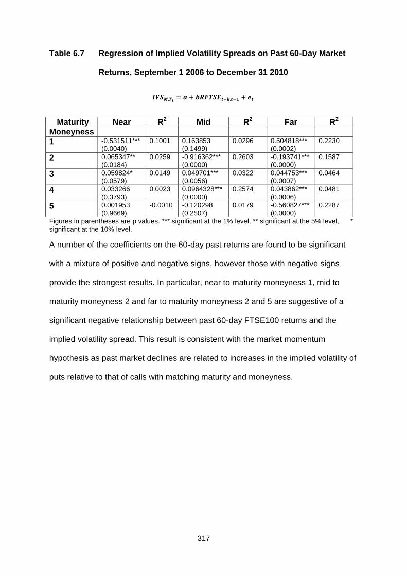
317

Table 6.7 Regression of Implied Volatility Spreads on Past 60-Day Market


Maturity Near R2 Mid R2 Far R2

Moneyness

1 -0.531511*** (0.0040)

0.1001 0.163853 (0.1499)

0.0296 0.504818*** (0.0002)

0.2230

2 0.065347** (0.0184)

0.0259 -0.916362*** (0.0000)

0.2603 -0.193741*** (0.0000)

0.1587

3 0.059824* (0.0579)

0.0149 0.049701*** (0.0056)

0.0322 0.044753*** (0.0007)

0.0464

4 0.033266 (0.3793)

0.0023 0.0964328*** (0.0000)

0.2574 0.043862*** (0.0006)

0.0481

5 0.001953 (0.9669)

-0.0010 -0.120298 (0.2507)

0.0179 -0.560827*** (0.0000)

0.2287

Figures in parentheses are p values. *** significant at the 1% level, ** significant at the 5% level, * significant at the 10% level.

A number of the coefficients on the 60-day past returns are found to be significant

with a mixture of positive and negative signs, however those with negative signs

provide the strongest results. In particular, near to maturity moneyness 1, mid to

maturity moneyness 2 and far to maturity moneyness 2 and 5 are suggestive of a

significant negative relationship between past 60-day FTSE100 returns and the

implied volatility spread. This result is consistent with the market momentum

hypothesis as past market declines are related to increases in the implied volatility of

puts relative to that of calls with matching maturity and moneyness.

318

6.3.3.1 Sub-Periods

Table 6.8 Regression of Implied Volatility Spreads on Past 60-Day Market Returns, Pre-Crisis; 1st January 2007- 31st May 2007

Maturity Near R2 Mid R2 Far R2

Moneyness

1 -0.005214 (0.9597)

-0.0104 1.006374*** (0.0002)

0.1643 0.252575*** (0.0006)

0.2186

2 -0.127237 (0.2802)

0.0114 -0.260631 (0.2532)

-0.0011 -0.006310 (0.8973)

-0.0095

3 -0.253757** (0.0493)

0.0524 0.142778 (0.1352)

0.0471 -0.064221 (0.2693)

0.0196

4 -0.422728*** (0.0041)

0.0935 0.323148 (0.3076)

0.0010 -0.045419 (0.3560)

0.0120

5 -0.679894*** (0.0007)

0.1337 -0.463425** (0.0294)

0.0680 -0.171292 (0.3073)

0.0192


The results presented in Table 6.8 indicate that, for the pre-crisis sub-period, nearest

to maturity options have negative coefficients although only those with moneyness 3,

4 and 5 are significant. Nevertheless this is an interesting result as these categories

contain at-the-money as well as in-the-money puts rather than out-of-the-money

options which have been highlighted in the literature reviewed in previous chapters

as having the greatest information content. The results for volatility spreads

constructed using out-of-the-money options which produce significant coefficients on

past returns show a positive relationship. In aggregate the results for the pre-crises

period are inconclusive with respect to the market momentum hypothesis.

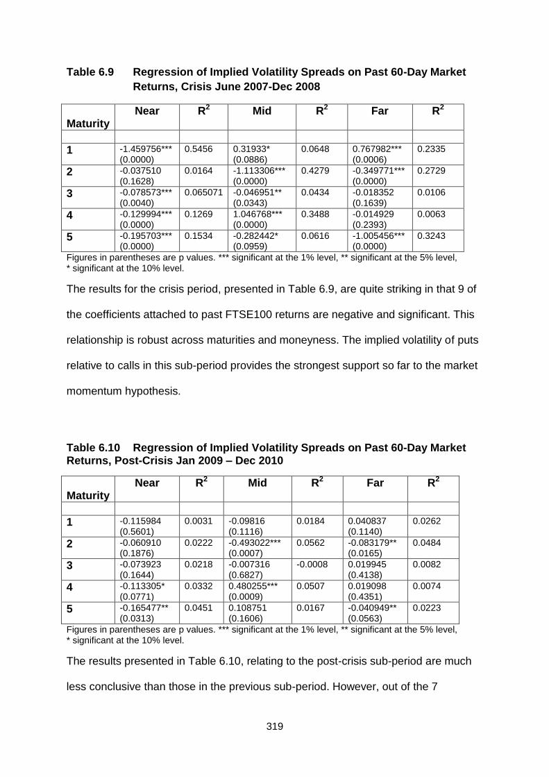
319

Table 6.9 Regression of Implied Volatility Spreads on Past 60-Day Market

Returns, Crisis June 2007-Dec 2008

Maturity

Near R2 Mid R2 Far R2

1 -1.459756*** (0.0000)

0.5456 0.31933* (0.0886)

0.0648 0.767982*** (0.0006)

0.2335

2 -0.037510 (0.1628)

0.0164 -1.113306*** (0.0000)

0.4279 -0.349771*** (0.0000)

0.2729

3 -0.078573*** (0.0040)

0.065071 -0.046951** (0.0343)

0.0434 -0.018352 (0.1639)

0.0106

4 -0.129994*** (0.0000)

0.1269 1.046768*** (0.0000)

0.3488 -0.014929 (0.2393)

0.0063

5 -0.195703*** (0.0000)

0.1534 -0.282442* (0.0959)

0.0616 -1.005456*** (0.0000)

0.3243


The results for the crisis period, presented in Table 6.9, are quite striking in that 9 of

the coefficients attached to past FTSE100 returns are negative and significant. This

relationship is robust across maturities and moneyness. The implied volatility of puts

relative to calls in this sub-period provides the strongest support so far to the market

momentum hypothesis.

Table 6.10 Regression of Implied Volatility Spreads on Past 60-Day Market Returns, Post-Crisis Jan 2009 – Dec 2010

Maturity

Near R2 Mid R2 Far R2

1 -0.115984 (0.5601)

0.0031 -0.09816 (0.1116)

0.0184 0.040837 (0.1140)

0.0262

2 -0.060910 (0.1876)

0.0222 -0.493022*** (0.0007)

0.0562 -0.083179** (0.0165)

0.0484

3 -0.073923 (0.1644)

0.0218 -0.007316 (0.6827)

-0.0008 0.019945 (0.4138)

0.0082

4 -0.113305* (0.0771)

0.0332 0.480255*** (0.0009)

0.0507 0.019098 (0.4351)

0.0074

5 -0.165477** (0.0313)

0.0451 0.108751 (0.1606)

0.0167 -0.040949** (0.0563)

0.0223


The results presented in Table 6.10, relating to the post-crisis sub-period are much

less conclusive than those in the previous sub-period. However, out of the 7

320

significant coefficients attached to past FTSE100 returns 6 are found to be negative.

The results are fairly evenly dispersed across maturity and moneyness and provide

some support, albeit weaker than from the previous sub-period, for the market

momentum hypothesis.

Overall the tests performed by regression 60-day past FTSE100 returns on implied

volatility spreads generated using FTSE100 options provide considerable support for

the market momentum hypothesis. It seems that demand does have a role to play in

the pricing of options.

6.4 Short-Run Overreaction

6.4.1 Introduction

This section further examines the relationship between past FTSE100 returns and

FTSE100 index option prices, under the assumption that demand is instrumental in

option pricing. In order to examine for overreaction, market price changes are

selected which are the most extreme in the sample and are over much shorter time

periods than the 60-day period analysed in the previous section. The objective is to

evaluate whether options investors exhibit short-term overreaction following sharp

movements in the FTSE100. It seems quite reasonable that option traders will be

much more inclined to write options conditional on recent stock price changes than

to write these unconditionally. The hypothesis is therefore that puts will become

overpriced following steep declines in the index and that, the more pronounced the

decline, the greater the overpricing. The same data set as used in the momentum

analysis is used for the overreaction tests. However, the testing procedure is

somewhat different and focuses on a measure of expensiveness. The measure of

expensiveness is given by the difference between implied volatility and ex post

321

realised volatility for the remaining life of the option. If implied volatility is significantly

and consistently different to ex post realised volatility this implies that options are

mispriced. For the purposes of this study the focus will be on whether implied

volatility exceeds ex post realised volatility both unconditionally and conditional on

sharp, short-term price changes in the underlying asset. Conditional excess volatility

relative to ex post realised volatility is employed by Gettleman, Julio and Risik (2011)

as a measure of expensiveness. If options are found to be consistently „expensive‟

following sharp, short-term changes in the value of the underlying asset then this is

interpreted as option traders overreacting to information. In this respect they

perceive a short sequence of price changes leading to a significant rise or fall in the

underlying asset as indicative of a trend.

The overreaction tests are performed in event time. Hence the options that are

included in the tests are selected conditional on recent underlying index returns. The

definition of an event relating to a broad market index is somewhat arbitrary. To

address this, 5-day return groups are sorted according to their magnitudes. The

sample is divided into deciles and ranked lowest to highest. Deciles 1, 2, 9 and 10

are analysed and are defined as follows:

Decile 1 – the most negative five day returns in the sample

Decile 2 – the second most negative five day returns in the sample

Decile 9 – the most positive five day returns in the sample

Decile 10 – the second most positive five day returns in the sample

After sorting a number of observations are removed from each of the examined

deciles to ensure no overlapping of events. The event windows are non-overlapping

322

in the sense that if an event occurs in a particular 5-day period, no subsequent event

period can begin until that 5-day period is complete.

Five categories of options are considered with category 1 being furthest in-the-

money, category 2 in-the-money, category 3 at- or close to-the-money, category 4

out-of-the-money and category 5 furthest out-of-the-money. This means that the

sample contains pairs of options with a variety of strike prices but maintains a

consistent relationship with the value of the underlying index throughout the entire

period. The measure of expensiveness is compared across each category with a

common maturity date. Only the most liquid options are included in the sample to

ensure the reliability of prices. The maturity of the options selected is a maximum of

six months with no options included with less than one week to expiration. Ex post

realised volatility is calculated as the volatility of the underlying asset over the

remaining life of the option subsequent to an extreme market movement. It is

computed as follows:

∑ √

(6.3)

Where rt is the daily return on the underlying asset

The analysis is performed using averages of implied volatility and expensiveness for

each maturity and moneyness combination. Expensiveness is defined as the

difference between implied volatility and the ex post realised volatility of the

underlying asset up to the maturity of the option under consideration. Tables 6.11

and 6.12 contain unconditional implied volatilities and measures of expensiveness

for each moneyness and maturity taken over the entire sample period. Tables 6.13

323

to 6.16 contain implied volatilities and moneyness measures conditional on past 5-

day returns.

Table 6.11 Unconditional Implied Volatilities

Moneyness 1 2 3 4 5

Panel A: Calls

Near 0.199616 0.199687 0.201523 0.208891 0.21877

Mid 0.305517 0.199778 0.199956 0.210888 0.296687

Far 0.189493 0.193956 0.198259 0.20112 0.241676

Average 0.231542 0.197807 0.199913 0.206966 0.252378

Panel B: Puts

Near 0.135532 0.217051 0.211578 0.209584 0.207989

Mid 0.317583 0.237265 0.225812 0.224878 0.341323

Far 0.2593 0.23946 0.247285 0.241923 0.238064

Average 0.237472 0.231259 0.228225 0.225462 0.262459

In most cases put implied volatilities exceed those of the corresponding calls. This

relationship is most pronounced, on average, for at-the-money and closest in-the-

money options. There is also clear evidence of a skewed volatility smile with the

smile for puts sitting above that for calls apart from one low paired observation for

nearest to maturity, deepest-in-the-money options.

The unconditional expensiveness indicates the magnitude of implied volatility relative

to ex post realised volatility up to the maturity of the option. A positive figure

indicates that the implied volatility exceeds the ex post realised volatility. It follows

that a positive figure identifies an option as being overpriced according to its implied

volatility.

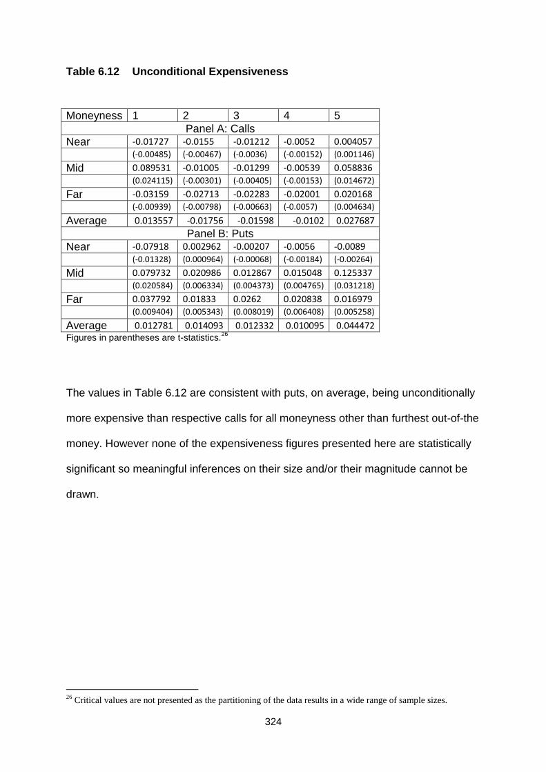
324

Table 6.12 Unconditional Expensiveness

Moneyness 1 2 3 4 5

Panel A: Calls

Near -0.01727 -0.0155 -0.01212 -0.0052 0.004057

(-0.00485) (-0.00467) (-0.0036) (-0.00152) (0.001146)

Mid 0.089531 -0.01005 -0.01299 -0.00539 0.058836

(0.024115) (-0.00301) (-0.00405) (-0.00153) (0.014672)

Far -0.03159 -0.02713 -0.02283 -0.02001 0.020168

(-0.00939) (-0.00798) (-0.00663) (-0.0057) (0.004634)

Average 0.013557 -0.01756 -0.01598 -0.0102 0.027687

Panel B: Puts

Near -0.07918 0.002962 -0.00207 -0.0056 -0.0089

(-0.01328) (0.000964) (-0.00068) (-0.00184) (-0.00264)

Mid 0.079732 0.020986 0.012867 0.015048 0.125337

(0.020584) (0.006334) (0.004373) (0.004765) (0.031218)

Far 0.037792 0.01833 0.0262 0.020838 0.016979

(0.009404) (0.005343) (0.008019) (0.006408) (0.005258)

Average 0.012781 0.014093 0.012332 0.010095 0.044472 Figures in parentheses are t-statistics.

26

The values in Table 6.12 are consistent with puts, on average, being unconditionally

more expensive than respective calls for all moneyness other than furthest out-of-the

money. However none of the expensiveness figures presented here are statistically

significant so meaningful inferences on their size and/or their magnitude cannot be

drawn.

26

Critical values are not presented as the partitioning of the data results in a wide range of sample sizes.

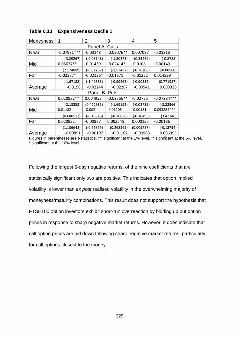
325

Table 6.13 Expensiveness Decile 1

Moneyness 1 2 3 4 5

Panel A: Calls

Near -0.07931*** -0.03148 -0.03076** 0.007087 -0.01213

(-3.29267) (-0.03148) (-1.80373) (0.55469) (-0.8788)

Mid 0.05627** -0.01459 -0.02414* -0.0108 -0.00149

(2.174889) (-0.81267) (-1.53437) (-0.76208) (-0.08568)

Far -0.02377* -0.02126* -0.01371 -0.01252 0.014599

(-1.67188) (-1.49585) (-0.99462) (-0.90552) (0.771987)

Average -0.0156 -0.02244 -0.02287 -0.00541 0.000326

Panel B: Puts

Near 0.020932** 0.004952 -0.02556** -0.02735 -0.07284***

(-2.13358) (0.422983) (-1.69192) (-0.02735) (-3.38366)

Mid 0.01182 -0.002 -0.01105 -0.00181 0.093884***

(0.686513) (-0.15515) (-0.76856) (-0.10495) (3.42346)

Far 0.020932 -0.00887 0.003545 0.000135 -0.00186

(1.106648) (-0.66855) (0.268569) (0.009787) (-0.13794)

Average -0.00891 -0.00197 -0.01102 -0.00968 0.006395 Figures in parentheses are t-statistics. *** significant at the 1% level, ** significant at the 5% level, * significant at the 10% level.

Following the largest 5-day negative returns, of the nine coefficients that are

statistically significant only two are positive. This indicates that option implied

volatility is lower than ex post realised volatility in the overwhelming majority of

moneyness/maturity combinations. This result does not support the hypothesis that

FTSE100 option investors exhibit short-run overreaction by bidding up put option

prices in response to sharp negative market returns. However, it does indicate that

call option prices are bid down following sharp negative market returns, particularly

for call options closest to the money.

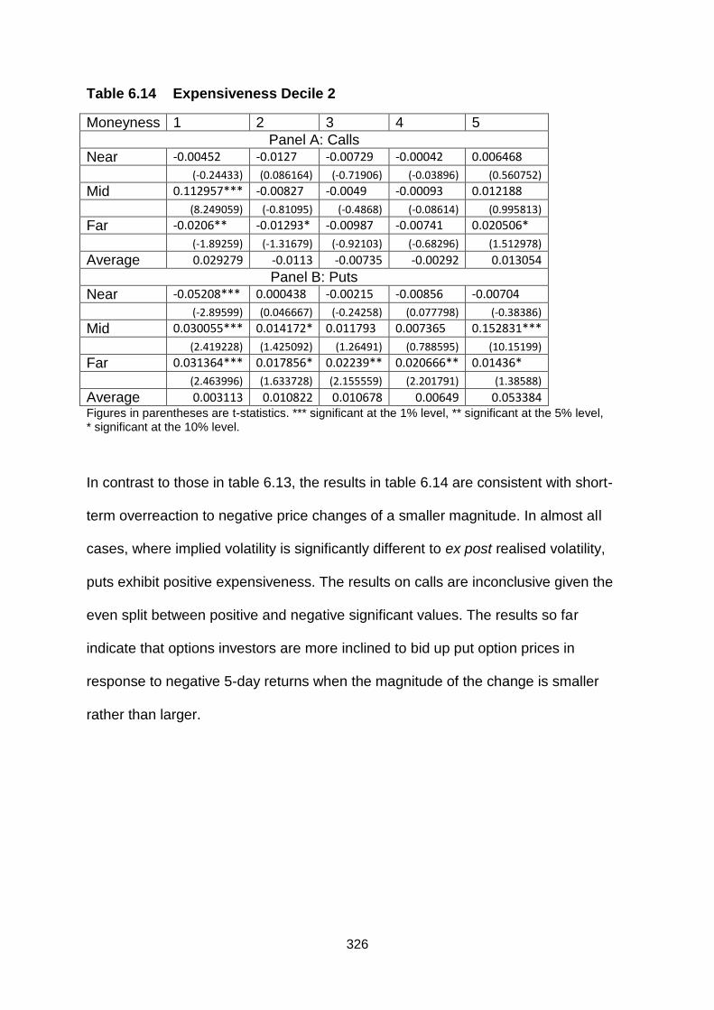
326


Moneyness 1 2 3 4 5

Panel A: Calls

Near -0.00452 -0.0127 -0.00729 -0.00042 0.006468

(-0.24433) (0.086164) (-0.71906) (-0.03896) (0.560752)

Mid 0.112957*** -0.00827 -0.0049 -0.00093 0.012188

(8.249059) (-0.81095) (-0.4868) (-0.08614) (0.995813)

Far -0.0206** -0.01293* -0.00987 -0.00741 0.020506*

(-1.89259) (-1.31679) (-0.92103) (-0.68296) (1.512978)

Average 0.029279 -0.0113 -0.00735 -0.00292 0.013054

Panel B: Puts

Near -0.05208*** 0.000438 -0.00215 -0.00856 -0.00704

(-2.89599) (0.046667) (-0.24258) (0.077798) (-0.38386)

Mid 0.030055*** 0.014172* 0.011793 0.007365 0.152831***

(2.419228) (1.425092) (1.26491) (0.788595) (10.15199)

Far 0.031364*** 0.017856* 0.02239** 0.020666** 0.01436*

(2.463996) (1.633728) (2.155559) (2.201791) (1.38588)

Average 0.003113 0.010822 0.010678 0.00649 0.053384 Figures in parentheses are t-statistics. *** significant at the 1% level, ** significant at the 5% level, * significant at the 10% level.

In contrast to those in table 6.13, the results in table 6.14 are consistent with short-

term overreaction to negative price changes of a smaller magnitude. In almost all

cases, where implied volatility is significantly different to ex post realised volatility,

puts exhibit positive expensiveness. The results on calls are inconclusive given the

even split between positive and negative significant values. The results so far

indicate that options investors are more inclined to bid up put option prices in

response to negative 5-day returns when the magnitude of the change is smaller

rather than larger.

327


Moneyness 1 2 3 4 5

Panel A: Calls

Near -0.01024* -0.00382 -0.00248 0.002781 0.007009

(-1.59155) (0.086771) (-1.10017) (-0.48858) (0.047069)

Mid 0.105102*** 0.004957* -0.00675 0.001267 0.017353

(5.790247) (-1.38289) (-1.18441) (-0.92569) (-0.49533)

Far -0.0111** -0.00748** -0.00635* -0.00443* 0.03014

(-2.17143) (-1.94877) (-1.41587) (-1.37167) (0.265096)

Average 0.027921 -0.00211 -0.00519 -0.00013 0.018167

Panel B: Puts

Near -0.04896*** 0.003692 -0.00126 -0.0028 -0.00625

(-2.5646) (-0.01203) (-0.59484) (0.0781) (-1.23719)

Mid 0.030697 0.011673 0.003722 0.015557 0.143081***

(1.021417) (0.455377) (0.243694) (0.039902) (7.341759)

Far 0.0337 0.008939 0.014286 0.016497 0.013436

(1.218581) (0.735573) (1.175691) (0.822241) (0.48241)

Average 0.005146 0.008101 0.005583 0.009751 0.050089 Figures in parentheses are t-statistics. *** significant at the 1% level, ** significant at the 5% level, * significant at the 10% level.

The results presented in table 6.15 do not provide support for the short-term

overreaction hypothesis. Expensiveness values for puts are only significant in two

instances, one positive and one negative, so no inferences can be drawn.

Furthermore, call implied volatility is not found to be consistently higher than ex post

realised volatility following the largest positive past 5-day returns on the FTSE100

index. Only mid to maturity in-the-money calls produce expensiveness values that

are positive and significant.

328


Moneyness 1 2 3 4 5

Panel A: Calls

Near -0.02067 -0.01309 -0.01169 -0.00529 0.007009

(-0.72343) (0.072143) (-0.25041) (0.264111) (0.641075)

Mid 0.084645*** -0.01622 -0.01323 -0.01051 -0.00641

(6.371722) (0.338969) (-0.59671) (0.099915) (1.126765)

Far -0.02421 -0.02161 -0.01538 -0.0162 0.002586**

(-0.99423) (-0.66902) (-0.52555) (-0.36272) (1.742325)

Average 0.013255 -0.01697 -0.01343 -0.01067 0.001062

Panel B: Puts

Near -0.04896** -0.00011 -0.00564 -0.00667 -0.0153

(-2.29877) (0.397759) (-0.14295) (0.064815) (-0.50201)

Mid 0.012805** 0.004741 0.0025 0.000442 0.115954***

(1.997335) (0.95941) (0.363331) (1.095013) (8.051304)

Far 0.011813 0.008259 0.012016 0.008613* 0.005062

(0.004503) (0.738945) (1.210976) (1.509802) (1.239264)

Average -0.00811 0.004297 0.002959 0.000795 0.035239 Figures in parentheses are t-statistics. *** significant at the 1% level, ** significant at the 5% level, * significant at the 10% level.

The results in table 6.16 are largely consistent with those in table 6.15 providing little

support for the short-term overreaction hypothesis. Although all of the significant

expensiveness values for calls have the expected sign, this only applies to two

observations. Three out of four significant put values have positive signs indicating

that investors appear more likely to bid up index put option prices following the

second-largest category of positive index returns. However, the large number of

insignificant values provides little support for the overreaction hypothesis.

In aggregate the results can, at best, be regarded as providing very weak support for

the overreaction hypothesis. This finding is in contrast to, but does not contradict,

that of Gettleman, Julio and Risik (2011) as they focus on the market for individual

equity options rather than index options.

The characteristics of the sample period, particularly the volatility of the market, may

go some way towards explaining the seemingly counter-intuitive results. One

329

possible explanation for the lack of positive and significant expensiveness figures for

put options when 5-day returns are most negative is the extremely high market

volatility in the second half of 2008.27 In order to test this explanation the data is

partitioned according to the pre-crisis, crisis and post-crisis periods defined earlier.

Unconditional implied volatility and unconditional expensiveness can then be

examined across each sub-period. It is not worthwhile further partitioning these sub-

periods due to the clustering of negative and positive returns. Results are presented

in tables 6.17 to 6.22.

Table 6.17 Unconditional Implied Volatilities Pre-Crisis Period

Moneyness 1 2 3 4 5

Panel A: Calls

Near 0.096883 0.090779 0.09033 0.092723 0.096572

Mid 0.15997 0.096323 0.097942 0.09803 0.097191

Far 0.094152 0.095084 0.094882 0.09166 0.095665

Average 0.117002 0.094062 0.094385 0.094138 0.096476

Panel B: Puts

Near 0.137843 0.130535 0.126482 0.128491 0.138379

Mid 0.148708 0.141539 0.140015 0.138601 0.190454

Far 0.152025 0.16066 0.156514 0.154282 0.154631

Average 0.146192 0.144245 0.141004 0.140458 0.161155

Table 6.17 indicates that implied volatilities of index puts exceed those of

corresponding index calls across the moneyness range for the pre-crisis period.

There is evidence of a negatively skewed volatility smile for puts although this is less

pronounced than that for the entire period.

27

For example UK market volatility in excess of 50% was regularly observed during the final third of 2008.

330

Table 6.18 Unconditional Expensiveness Pre-Crisis Period

Moneyness 1 2 3 4 5

Panel A: Calls

Near -0.0046 -0.01034 -0.01067 -0.0085 -0.00626

(-0.00922) (-0.02224) (-0.0221( (-0.01759) (-0.01252)

Mid 0.053284 -0.01043 -0.00874 -0.00821 -0.0095

(0.077795) (-0.03049) (-0.02516) (-0.02387) (-0.02564)

Far -0.04186 -0.04093 -0.04113 -0.04435 -0.04084

(-0.06527) (-0.08209) (-0.08196) (-0.08765) (-0.07325)

Average 0.002275 -0.02057 -0.02018 -0.02035 -0.01887

Panel B: Puts

Near 0.03501 0.029308 0.02548 0.027367 0.036898

(0.073343) (0.059567) (0.04923) (0.053251) (0.064345)

Mid 0.042022 0.035304 0.033329 0.031847 0.083768

(0.113442) (0.097324) (0.090835) (0.089114) (0.15937)

Far 0.015518 0.02465 0.020501 0.018269 0.018618

(0.028365) (0.050095) (0.041623) (0.037312) (0.144804)


None of the values presented in table 6.18 are statistically significant. This means

that neither calls nor puts are overpriced according to the measure of

expensiveness. The clear inference is that implied volatility is not significantly

different to ex post realised volatility in the pre-crisis period.

Table 6.19 Unconditional Implied Volatilities Crisis Period

Moneyness 1 2 3 4 5

Panel A: Calls

Near 0.220463 0.222243 0.223989 0.229999 0.234711

Mid 0.349064 0.22643 0.220124 0.240304 0.262316

Far 0.209368 0.213744 0.217868 0.22132 0.312064

Average 0.259632 0.220806 0.22066 0.230541 0.269697

Panel B: Puts

Near 0.173735 0.265647 0.2623 0.260673 0.253102

Mid 0.310175 0.283444 0.262393 0.26831 0.371556

Far 0.326869 0.25251 0.277477 0.271729 0.267356

Average 0.27026 0.2672 0.26739 0.266904 0.297338

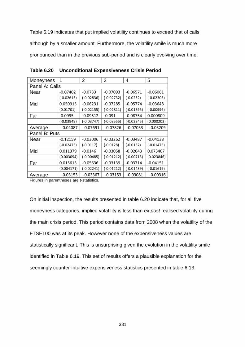
331

Table 6.19 indicates that put implied volatility continues to exceed that of calls

although by a smaller amount. Furthermore, the volatility smile is much more

pronounced than in the previous sub-period and is clearly evolving over time.

Table 6.20 Unconditional Expensiveness Crisis Period

Moneyness 1 2 3 4 5

Panel A: Calls

Near -0.07402 -0.0733 -0.07093 -0.06571 -0.06061

(-0.02615) (-0.02836) (-0.02732) (-0.0252) (-0.02303)

Mid 0.050915 -0.06231 -0.07285 -0.05774 -0.03648

(0.01701) (-0.02155) (-0.02811) (-0.01895) (-0.00996)

Far -0.0995 -0.09512 -0.091 -0.08754 0.000809

(-0.03949) (-0.03747) (-0.03555) (-0.03345) (0.000203)

Average -0.04087 -0.07691 -0.07826 -0.07033 -0.03209

Panel B: Puts

Near -0.12159 -0.03006 -0.03262 -0.03487 -0.04138

(-0.02473) (-0.0117) (-0.0128) (-0.0137) (-0.01475)

Mid 0.011379 -0.0146 -0.03058 -0.02043 0.073407

(0.003094) (-0.00485) (-0.01212) (-0.00715) (0.023846)

Far 0.015613 -0.05636 -0.03139 -0.03714 -0.04151

(0.004171) (-0.02241) (-0.01212) (-0.01439) (-0.01619)

Average -0.03153 -0.03367 -0.03153 -0.03081 -0.00316 Figures in parentheses are t-statistics.

On initial inspection, the results presented in table 6.20 indicate that, for all five

moneyness categories, implied volatility is less than ex post realised volatility during

the main crisis period. This period contains data from 2008 when the volatility of the

FTSE100 was at its peak. However none of the expensiveness values are

statistically significant. This is unsurprising given the evolution in the volatility smile

identified in Table 6.19. This set of results offers a plausible explanation for the

seemingly counter-intuitive expensiveness statistics presented in table 6.13.

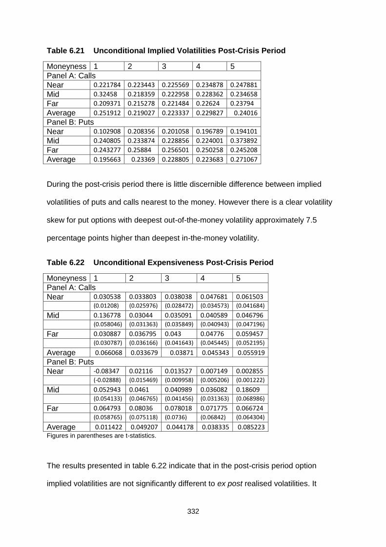
332

Table 6.21 Unconditional Implied Volatilities Post-Crisis Period

Moneyness 1 2 3 4 5

Panel A: Calls

Near 0.221784 0.223443 0.225569 0.234878 0.247881

Mid 0.32458 0.218359 0.222958 0.228362 0.234658

Far 0.209371 0.215278 0.221484 0.22624 0.23794

Average 0.251912 0.219027 0.223337 0.229827 0.24016

Panel B: Puts

Near 0.102908 0.208356 0.201058 0.196789 0.194101

Mid 0.240805 0.233874 0.228856 0.224001 0.373892

Far 0.243277 0.25884 0.256501 0.250258 0.245208

Average 0.195663 0.23369 0.228805 0.223683 0.271067

During the post-crisis period there is little discernible difference between implied

volatilities of puts and calls nearest to the money. However there is a clear volatility

skew for put options with deepest out-of-the-money volatility approximately 7.5

percentage points higher than deepest in-the-money volatility.

Table 6.22 Unconditional Expensiveness Post-Crisis Period

Moneyness 1 2 3 4 5

Panel A: Calls

Near 0.030538 0.033803 0.038038 0.047681 0.061503

(0.01208) (0.025976) (0.028472) (0.034573) (0.041684)

Mid 0.136778 0.03044 0.035091 0.040589 0.046796

(0.058046) (0.031363) (0.035849) (0.040943) (0.047196)

Far 0.030887 0.036795 0.043 0.04776 0.059457

(0.030787) (0.036166) (0.041643) (0.045445) (0.052195)

Average 0.066068 0.033679 0.03871 0.045343 0.055919

Panel B: Puts

Near -0.08347 0.02116 0.013527 0.007149 0.002855

(-0.02888) (0.015469) (0.009958) (0.005206) (0.001222)

Mid 0.052943 0.0461 0.040989 0.036082 0.18609

(0.054133) (0.046765) (0.041456) (0.031363) (0.068986)

Far 0.064793 0.08036 0.078018 0.071775 0.066724

(0.058765) (0.075118) (0.0736) (0.06842) (0.064304)


The results presented in table 6.22 indicate that in the post-crisis period option

implied volatilities are not significantly different to ex post realised volatilities. It

333

should also be highlighted that the post-crisis period contains the first quarter of

2009 during which high market volatility persisted. Option prices appear to be priced

highly yet consistently with the high volatility that was a feature of this period.

It is clear from the preceding analysis that there is no evidence of unconditional

overreaction of FTSE100 traders to FTSE100 returns. The evolution of the volatility

smile indicates that, unconditionally, option traders price options broadly in line with

ex post realised volatility.

6.5 Discussion and Conclusion

This chapter has provided an analysis of momentum and short-term overreaction

effects in the FTSE100 index options market around the time of the 2007/8 financial

crisis.

Model-independent tests for violations of the put-call boundary condition for

European-style FTSE100 options following 60-day market returns along with

parametric tests of implied volatility spreads are carried out. The results of the put-

call boundary violation tests provide some support for the market momentum

hypothesis although this is fairly weak. Stronger support is provided by the results of

regressions of the implied volatility spread on 60-day FTSE100 returns. These

results are interpreted as indicating a role for a demand parameter in option pricing.

The difference between implied volatility and realised volatility of the FTSE100,

conditional on significant index price moves, is examined as a measure of

expensiveness. These price movements are sorted into deciles with the two most

negative and two most positive selected as containing events. Fairly weak evidence

of conditional short-term overreaction is found, although in no way can this be

334

interpreted as consistent. This relationship is strongest following the second most

negative 5-day price movements (decile 2).

There is no evidence of unconditional overreaction because no significant

divergence between implied volatility and ex post realised volatility is identified. This

result is holds for the entire sample period as well as the pre-crisis, crisis and post-

crisis sub-periods. It does not seem that options market investors overreact

unconditionally to information at an aggregate level. One possible future extension to

this work would be to examine for short-term conditional overreaction using

individual equity options traded on Euronext LIFFE.

The volatility smile for options evolves in line with the volatility of the underlying

market and is consistent with a negatively skewed risk-neutral distribution.

Furthermore put options have consistently higher implied volatilities than call options

matched by moneyness and maturity.

Overall, the findings of this chapter support those of Amin, Coval and Seyhun (2004)

in inferring a role for demand in option pricing. However, little support is offered for

the findings of Gettleman, Julio and Risik (2011). As a consequence, this chapter

provides no motivation to construct a portfolio of FTSE100 options and underlying

stocks to test whether it is possible to generate systematic profits. If no evidence can

be found of short term overreaction it is not possible to form contrarian portfolios.

335

Chapter 7

Summary, Conclusions and Suggestions

for Future Research

336

7.1 Summary of Issues and Key Contributions

A substantial body of literature has been published that runs counter to the

neoclassical paradigm and, in particular rejects the conclusion of an efficient capital

market. Furthermore literature has been published which produces evidence in

derivative markets which supports the findings in the equity market. In aggregate this

literature provides the basis of the behavioural finance paradigm. To address all of

the contributions would take several volumes. However, key contributions and

subject areas have been covered in this thesis.

A debate between the proponents of efficient markets and those of behavioural

finance has continued for over 25 years with little agreement. The debate which was

initially focused on the equity market has more recently been extended to the options

market and focuses on the key areas of relative pricing, implied volatility and trading

behaviour. To date the overwhelming majority of published work has focused on the

United States market with data normally sourced from the Chicago Board Options

Exchange. The four empirical chapters in this thesis comprise the key areas of

options market research with data sourced from Euronext LIFFE for options traded in

London. Furthermore the analysis in each chapter is applied to one of the most

turbulent decades in financial history encompassing the inflation and subsequent

bursting of the dotcom bubble and the liquidity and banking crisis precipitated by the

sub-prime lending debacle. The combination of a UK-based study and application to

major financial crises makes this work an important contribution to the behavioural

finance literature. There is apparently little or no existing literature with this particular

focus.

337

Options provide a means by which to hedge against or speculate on future moves in

the price of the corresponding underlying assets. Option writers need some objective

parameters by which to price options based on the probability that they will

encounter a negative cash flow on exercise/expiry and, if a negative cash flow is

encountered, the magnitude of the flow. Academic research has produced a number

of models to calculate a fair option price based on observable parameters. Notable

models are those of Black, Scholes and Merton (1973) and Cox, Ross and

Rubinstein (1979). Attempts have been made to build on this work including

prominent models which are able to incorporate stochastic volatility such as those of

Hull and White (1987) and Heston (1993). However, the degree of pricing accuracy

has not improved greatly despite the proliferation of stochastic volatility models. The

one parameter in option pricing models which must be computed is volatility.

Volatility has proved to be so problematic that option traders regularly use implied

volatility of short-dated at-the-money options to price in- or out-of-the-money and

longer-dated options on the assumption that the market price is correct. However

this technique is still model-dependent. One key aspect of option pricing is the notion

of the option as a redundant asset with cash flows that can be replicated by a

combination of risky assets. Hence risk preferences are not included in the models

and options are priced under the assumption of risk-neutrality and frictionless

markets. If the sentiment of investors is a partial determinant of option price then it

will be apparent directly in the relative pricing of puts and calls or indirectly in model-

dependent implied volatility. It follows that an opportunity to test this proposition

arises in periods of significant market upheaval by examining the relative prices of

put and call options with strike prices symmetrically distributed around the price of

the underlying asset.

338

The first empirical chapter in this thesis extended existing research by examining

relative put and call prices in the UK index options market over the dotcom bubble

period at the turn of the century. The key finding presented in this chapter is that

relative option prices and associated implied volatility incorporated the negative

expectations of investors at the time of the dotcom bubble. However, this relationship

was found to persist during periods of relative tranquillity in markets, supporting the

assertion of Rubinstein (1994) that investors suffer from „crashophobia‟. The

calculation of a volatility spread and plotting of the behaviour of the volatility smile

across the sample period provided insights into investor behaviour and illustrated the

difficulties that option prices with lognormal risk-neutral distributions encounter in

pricing index options.

One of the most basic human emotions is fear. The great fear of stock market

investors or portfolio managers is that they may lose a substantial amount of the

value of their portfolios. Whaley (2000) proposes that this fear in the US is captured

by the VIX; an index of implied volatility constructed using options traded on the S&P

500 stock index. Numerous studies have analysed the VIX as a market consensus

view of future volatility whilst some have examined it as a predictor of stock market

returns. The literature reveals a significant role in volatility forecasting but is much

less clear on return predictability. Again, the bulk of the literature is focused on

volatility indexes in the US. The UK presents a gap in the literature as the

corresponding volatility index constructed from FTSE100 index options, the VFTSE,

was introduced fairly recently. This study provides a unique contribution to the

literature as a volatility index is constructed which permits analysis of the UK fear

gauge prior to the 2008 introduction of the VFTSE. In Chapter 4, the second

empirical chapter, a volatility index is constructed, the VUK, using FTSE100 option

339

implied volatilities from 2006 to 2010. A range of tests is applied to establish the

relationship between the VUK and the underlying large capitalisation market. Clear

evidence is produced to support the notion of the VUK as an index that reflects the

fear of UK investors. Furthermore, the VUK is found to be a good, although biased,

predictor of the future volatility of FTSE100 returns. No clear evidence of FTSE100

return predictability is found using the VUK indicating that the index is unable to

provide any indication of exploitable trading opportunities, at least when daily prices

are observed. Hence analysis of the VUK does not produce any evidence that

contradicts the efficient markets hypothesis. This represents an important finding

because no support for the behavioural finance paradigm is found using UK data in

this respect. The behaviour of the VUK is found to be fairly consistent across the

financial crisis. The clear negative correlation with index returns supports the notion

of the VUK as a fear index. Finally the VUK is found to be mean-reverting.

The third empirical chapter focuses on the third key behavioural issue in options

markets; trading behaviour. A number of studies find that patterns of trading

behaviour provide insights into investor sentiment. A prominent and thorough

example is that of Lakonishok, Lee and Poteshman (2003). A frequent observation is

that increases in trading volume and open interest are related to negative spot

market returns. Again the overwhelming majority of published literature is focused on

US markets. The important contribution to the literature provided by this study is an

analysis of the relationship between trading volume/open interest and the UK stock

market during the recent financial crisis. The empirical chapter first examines the

FTSE100 index and index options but then extends the analysis to a portfolio of

financial stocks that have exchange-traded options written on them. This

disaggregation is motivated by an expectation that the impact of the financial crisis is

340

likely to be greater than that on the aggregate market. Option portfolios are further

disaggregated by constraining the sample to include only out-of-the-money options.

The findings of Chapter 4 are supported in that little evidence of return predictability

is found. Again, this is an important finding which adds further weight to the case for

market efficiency. Some evidence is presented to support the price discovery role of

trading volume. Taken together these findings are consistent with the efficient

markets hypothesis. The most important finding in this chapter regards the change in

investor behaviour in response to a series of return innovations of the same sign as

opposed to a single return innovation. The put/call ratios of trading volume and of

open interest are shown to be negatively and significantly related to

contemporaneous spot market returns when there are three or more return

innovations of the same sign. However, no significant relationship is found between

the put/call ratios and daily innovations. This finding provides a clear indication that

UK investors are subject to conservatism and the representative heuristic. It seems

that the behavioural biases commonly observed in the equity market are also

present in the options market.

The fourth empirical chapter examines for evidence of momentum effects and

overreaction in the UK index options market over the financial crisis period of 2007/8.

Both a non-parametric approach and a parametric approach are employed to test for

momentum effects. Boundary condition violations and the behaviour of implied

volatility spreads are examined following 60-day positive and negative returns and

produce evidence supporting the momentum effect in the FTSE100 options market.

Overall, the findings of this chapter support those of Amin, Coval and Seyhun (2004)

in inferring a role for demand in option pricing.

341

Tests for short-run overreaction, conditional on sharp changes in the FTSE100 over

a preceding 5-day period, fail to provide compelling evidence that the UK index

options market overreacts. Hence, little support is offered for the findings of

Gettleman, Julio and Risik (2011). As a consequence, this chapter provides no

motivation to construct a portfolio of FTSE100 options and underlying stocks to test

whether it is possible to generate systematic profits.

Ultimately the achievement of this thesis has been to provide a thorough analysis of

behavioural finance in the context of options market behaviour in the UK. The

empirical results suggest that behavioural biases exist in UK markets but that the

market tends towards efficiency.

6.2 Future Research

This thesis has provided numerous insights into investor behaviour in UK markets

and consequently provides an important contribution to the literature. It is imperative

that this thesis provides a foundation for future research. For example, exchange-

traded options in other European markets and markets further afield provides a rich

source of data for broader analysis. If a Euronext.LIFFE database could be produced

that disaggregates data in a similar way to that provided by the CBOE it would

provide the opportunity for a huge step forward in investigating the behaviour of

market participants with varying degrees of sophistication. Furthermore there may be

insights into momentum and overreaction effects in equity option data which cannot

be found in index option data.

342

Bibliography

Aguirre, M.S., Saidi, R., 1999. Feedback trading in exchange-rate markets: evidence

from within and across economic blocks, Journal of Economics and Finance 23, 1-

14.

Allais, M., 1953. The behaviour of rational man in risk situations – a critique of the

axioms and postulates of the American school. Econometrica 21, 503-546.

Allen, F., Gorton, G., 1991. Rational finite bubbles. NBER Working Paper, Number

3707.

Amir, E., Ganzach, Y., 1998. Overreaction and underreaction in analysts‟ forecast. Journal of Economic Behaviour and Organisation 37, 333-347.

Amin, K.I., Lee, C.M.C., 1997. Option trading, price discovery and earnings news dissemination. Contemporary Accounting Research 14, 153-192.

Amin, K.I., Coval, J., Seyhun, H.N., 2004. Index option prices and stock market

momentum. Journal of Business 77, 835-873.

Andergassen, R., 2005. Rational destabilising speculation and the rising of bubbles. Journal of Behavioural Finance 2, 69-83.

Antoniou, A., Galariotis, E., Spyrou, S., 2005. Contrarian profits and the overreaction hypothesis: the case of the Athens Stock Exchange. European Financial Management 11, 71-98.

Areal, N.M.P.B.C, 2008. FTSE-100 implied volatility index. NEGE Working Paper.

Ariel, R.A., 1990. High stock returns before holidays: existence and evidence on possible causes. Journal of Finance 45, 1611-1626.

Assoe, K., Sy, O., 2003. Profitability of the short-run contrarian strategy in Canadian stock markets. Canadian Journal of Administrative Sciences 20, 311-319.

Bachelier, L., 1900. Théorie de la spéculation. Annales Scientifiques de l’École

Normale Supérieure 3, 21-86.

Baker, M., Wurgler, J., 2000. The equity share in new issues and aggregate stock returns. Journal of Finance 55, 2219-2258.

Baker, M., Wurgler, J., 2004. A catering theory of dividends. Journal of Finance 59, 1125-1165.

Bakshi, G., Cao, C., and Chen, Z., 1997. Empirical performance of alternative option

pricing models. Journal of Finance, 52, 2003-2049.

Ball, R., 1978. Anomalies in relationships between securities‟ yields and yield

surrogates. Journal of Financial Economics, 6, 103-126.

343

Ball, R., Kothari, S., 1989. Nonstationary expected returns: implications for tests of

market efficiency and serial correlation in returns. Journal of Financial Economics 25,

51-74.

Bandi, F.M., Perron, B., 2006. Long memory and the relation between implied and

realized volatility. Journal of Financial Econometrics, 4, 636-670.

Barber, B., and Odean, T., 2000. Trading is hazardous to your wealth: The common stock investment performance of individual investors. Journal of Finance 55, 773-806. Barber, B., and Odean, T., 2001. Boys will be boys: Gender, overconfidence, and common stock investment. Quarterly Journal of Economics 116, 261-292. Barber, B., and Odean, T., 2002. Online investors: do the slow die first? Review of Financial Studies 15, 455-487. Barberis, N., Huang, M., Santos, T., 2001. Prospect theory and asset prices. Quarterly Journal of Economics 116, 1-53. Barberis, N., Huang, M., 2008. Stocks as lotteries: the implications of probability weighting for security prices. American Economic Review 98, 2066-2100. Barberis, N., Shleifer, A., Vishny, R., 1998. A model of investor sentiment. Journal of Financial Economics 49, 307-343.

Barberis, N., Shleifer, A., Wurgler, J., 2003. Comovement. Journal of Financial Economics 75, 283-317.

Barberis, N., Thaler, R., 2002. A survey of behavioral finance. NBER working paper

9222.

Barberis, N., Xiong, W., 2009. What drives the disposition effect? An analysis of a

long-standing preference-based explanation, Journal of Finance 66, 751-784.

Barraclough, K., Whaley, R.E., 2012. Early exercise of put options on stocks Journal

of Finance 67, 1423-1456.

Bates, D., 1991. The crash of '87: was it expected? The evidence from options

markets. Journal of Finance 46, 1009-1044.

Bates, D., 1997. Post-'87 crash fears in S&P 500 futures options. NBER working

paper 5894.

Bates, D.S., 2003. Empirical option pricing: a retrospection. Journal of Econometrics

116, 387-404.

344

Bekiros, S.D., Georgoutsos, D.A., 2008. Non-linear dynamics in financial asset returns: the predictive power of the CBOE volatility. The European Journal of Finance, 14, 397-408.

Berk, J.B., Green, R.C., 2004. Mutual fund flows and performance in rational

markets. Journal of Political Economy 112, 1269-1295.

Berk, J.B., Stanton, R., 2007. Managerial ability, compensation and the closed-end

fund discount. Journal of Finance 62, 529-556.

Bernard, V., 1992. Stock price reactions to earnings announcements: a summary of

recent anomalous evidence and possible explanations, in Thaler, R., ed, Advances

in Behavioural Finance. Russell Sage Foundation, New York, 303-340.

Bernard, V., Thomas, J., 1990. Evidence that stock prices do not fully reflect the

implications of current earnings for future earnings. Journal of Accounting and

Economics 13, 305-340.

Bernartzi, Thaler, R. 1995. Myopic loss aversion and the equity premium puzzle.

Quarterly Journal of Economics 110, 73-92.

Bhattacharya, M., 1980, Empirical properties of the Black-Scholes formula under

ideal conditions. Journal of Financial and Quantitative Analysis 15, 1081–1105.

Bhattacharya, M., 1983. Transactions data tests of efficiency of the Chicago Board

Options Exchange, Journal of Financial Economics 12, 161-185.

Bikchandani, S., Sharma, S., 2000. Herd behaviour in financial markets: a review.

IMF Staff Papers 48.

Black, F., 1972. Capital market equilibrium with restricted borrowing. Journal of

Business 45, 444-455.

Black, F., 1975. Fact and fantasy in the use of options. Financial Analysts Journal

31, 36-72.

Black, F., 1986. Noise. Journal of Finance 41, 529-543.

Black, F., 1989. How to use the holes in Black-Scholes. Journal of Applied Corporate

Finance 1, 67-73.

Black, F., Scholes, M., 1972. The valuation of option contracts and a test of market

efficiency. Journal of Finance 27, 399-418.

Black, F., Scholes, M., 1973. The pricing of options and corporate liabilities. Journal

of Political Economy 81, 637-659.

345

Blair, B.J., Poon, S.H., Taylor, S. 2001. Forecasting S&P 100 volatility: the

incremental information content of implied volatilities and high-frequency index

returns. Journal of econometrics, 105, 5-26.

Bodurtha, J., Courtadon, G., 1986. Efficiency of the foreign currency options market.

Journal of Finance, 41, 151-162.

Bohl, M.T., Reitz, S., 2006. Do positive feedback traders act on Germany‟s Neuer

market? Quarterly Journal of Business and Economics 44, 3-14

Bollen, N.P.B., Whaley, R.E., 2004. Does net buying pressure affect the shape of

implied volatility functions? Journal of Finance 59, 711-753.

Bondarenko, O., 2003. Why are put options so expensive? University of Illinois at

Chicago Working Paper.

Bowman, R., Iverson, D., 1998. Short-run overreaction in the New Zealand stock

market. Pacific-Basin Finance Journal 6, 475-491.

Brandt, M.W., Wu, T., 2002. Cross-sectional tests of deterministic volatility functions.

Journal of Empirical Finance 9, 525-550.

Brauer, G.A., Chang, E., 1990. Return seasonality in stocks and their underlying

assets: tax loss selling versus information explanations. Review of Financial Studies

3, 257-280.

Bremer, M., Hiraki, T., 1999. Volume and individual security returns on the Tokyo

Stock Exchange. Pacific-Basin Finance Journal 7, 351-370.

Burashi, A., Jiltsov, A., 2006. Model uncertainty and option markets with heterogeneous beliefs. Journal of Finance 61, 2841-2897.

Campbell, J.Y., 1991. A variance decomposition for stock returns. Economic Journal

101, 157-179.

Campbell, J.Y., Kyle, A.S., 1993. Smart money, noise trading and stock price

behaviour. Review of Economic Studies 60, 1-34.

Campbell, J.Y., Lo, A.W., Mackinlay, A.C., 1997. The Econometrics of Financial

Markets. New Jersey: Princeton University Press.

Campbell, J.Y., Shiller, R.J., 1988. Stock prices, earnings and expected dividends.

Journal of Finance 43, 661-676.

Canina, L., Figlewski, S. 1993, The informational content of implied volatility. Review

of Financial Studies 6 (3), 659-681.

Cao, C., Chen, Z., Griffin, J.M., 2005, Informational content of option volume prior to

takeovers. Journal of Business 78, 1073-1109.

346

Cao, C., Li, H., Yu, F., 2005, Is investor misreaction economically significant?

Evidence from short- and long-term S&P 500 index options. Journal of Futures

Markets 25, 717-752.

Cao, M., Wei, J., 2005. Stock market returns: a note on temperature anomaly.

Journal of Banking and Finance 29, 1559-1573.

Cao, H.C., Yang, H.O., Differences of opinion of public information and speculative

trading in stocks and options. Review of Financial Studies 22, 299-335.

Chakraverty, S., Gulen, H., Mayhew. S., 2004, Informed trading in stock and options

markets. Journal of Finance 59, 1235-1257.

Chan, K.C., 1988. On the contrarian investment strategy Journal of Business 61,

147-164.

Chan, K., Chung, P., Fong, W.M., 2002, The informational role of stock and option

volume. Review of Financial Studies 15, 1049-1075.

Chan. L., Jegadeesh, N., Lakonishok, J., 1997. Momentum strategies. Journal of

Finance 51, 1681-1713.

Chang, E.C., Cheng, J.W., Khorana, A., 2000. An examination of herd behaviour in

equity markets: an international perspective. Journal of Banking and Finance 24,

1651-1679.

Chancellor, E., 2000. The Devil Take the Hindmost: A History of Financial

Speculation. London: Macmillan.

Chang, C-C., Hsieh, P-F., Lai, H-N., 2009. Do informed option investors predict stock

returns? Evidence from the Taiwan Stock Exchange. Journal of Banking and

Finance 33, 757-764.

Chang, R.P., Mcleavey, D.W., Rhee, S.G., 1995. Short-term abnormal returns of the

contrarian strategy in the Japanese stock market. Journal of Business, Finance and

Accounting 22, 1035-1048.

Chen, H-L., Jegadeesh, N., Wermers, R., 2000. The value of active mutual fund

management: an examination of the stockholdings and trades of fund managers.

Journal of Financial and Quantitative Analysis 35, 343-368.

Chen, J., Hong, H., Stein, J.C., 2001. Forecasting crashes: trading volume, past

returns, and conditional skewness in stock prices. Journal of Financial Economics

61, 345-381.

Chen, N-F, Roll, R., Ross, S., 1986. Economic forces and the stock market. Journal

of Business 59, 383-403.

347

Cherkes, M., Sagi, J., Stanton, R., 2009. A liquidity-based theory of closed-end

funds. Review of Financial studies 22, 257-297.

Chernov, M., Ghysels, E., 2000. A study towards a unified approach to the joint

estimation of objective and risk neutral measures for the purpose of options valuation.

Journal of Financial Economics 56, 407-458.

Chiras, D., Manaster, S. 1978. The information content of option prices and a test of

market efficiency. Journal of Financial Econometrics 6, 213-234.

Christensen, B.J., Prabhala, N.R., 1998. The relation between implied and realized

volatility. Journal of Financial Economics 50 (2) 125-150.

Christie, W.G., Huang, R.D., 1995. Following the Pied Piper: do individual returns

herd around the market? Financial Analysts Journal 51, 31-37.

Clare, A., Thomas, S., 1995. The overreaction hypothesis and the UK stock market.

Journal of Business, Finance and Accounting 22, 961-973.

Conrad, J., Kaul, G., 1993. Long-term market overreaction or biases in computed

returns? Journal of Finance 48, 39-63.

Conrad, J., Gultekin, M., Kaul, G., 1993. Asymmetric predictability of conditional

variances. Review of Financial Studies 4, 597-622.

Conrad, J., Gultekin, M., Kaul, G., 1997. Profitability of short-term contrarian

strategies: implications for market efficiency. Journal of Business and Economic

Statistics 15, 379-386.

Constantinides, G.M., 1983. Capital market equilibrium with personal tax.

Econometrica 51, 3, 611-636.

Constantinides, G.M., 1990. Habit formation: a resolution of the equity premium

puzzle. Journal of Political Economy 98, 519-543.

Constantinides, G.M., Donaldson, J.B., Mehra, R., 2002. Junior can‟t borrow: a new

perspective on the equity premium puzzle.

Constantinides, G. M., Jackwerth, J. C., and Savov, A. Z., 2011. The Puzzle of Index Option returns, University of Chicago Working Paper.

Coval, J.D., Shumway, T., 2001. Expected option returns. Journal of Finance 56, 983-1009. Cox, J.C., Ross, S.A., Rubinstein, M., 1979. Option pricing: a simplified approach.


Cremers, M., Weinbaum, D., 2010. Deviations from put-call parity and stock return

predictability. Journal of Financial and Quantitative Analysis 45, 335-367.

348

Cuthbertson, C., Nitzsche, D., 2001. Financial Engineering. Chichester: Wiley.

Cutler, D.M., Poterba, J.M., Summers, L.H., 1991. Speculative dynamics. Review of

Economic Studies 58, 529-546.

Da Costa, J., Newton, C.A., 1994. Overreaction in the Brazilian stock market.

Journal of Banking and Finance, 18, 633-642.

Daniel, K.D., Hirshleifer, D., Subrahmanyam, A., 1998. Investor psychology and

security market under- and over-reactions, Journal of Finance 53, 1839-1886.

Das, S.R., Sundaram, R.K., 1999. Of smiles and smirks: a term structure

perspective. Journal of Financial and Quantitative Analysis 34, 211-239.

Dawson, P., 1996. Rational early exercise of equity and index options: the impact of

market frictions. Journal of Business Finance and Accounting 23, 931-951.

Day, T.E., Lewis, C.M., 1992. Stock market volatility and the informational content of

stock index options. Journal of Econometrics, 52, 267-287.

De Bondt, W., Thaler, R., 1985. Does the stock market overreact?, Journal of

Finance vol 40, no 3, 793-805.

De Bondt, W., Thaler, R., 1987. Further evidence on investor overreaction and stock

market seasonality, Journal of Finance 42, 557-581.

De Long, J.B., Shleifer, A., Summers, L.H., Waldmann, R.J., 1990. Positive feedback investment strategies and destabilising rational speculation. Journal of Finance 45, 379-395.

Devenow, A., Welch, I., 1996. Rational herding in financial economics. European

Economic Review 40, 603-615.

Dewally, M., 2003. Internet investment advice: investing with a rock of salt. Financial

Analysts Journal 59, 65-77.

Dissanaike, G., 1997. Do stock market investors overreact? Journal of Business

Finance and Accounting 24, 27-49.

Diz, F., Finucane, T.J., 1993. The rationality of early exercise decisions: evidence

from the S&P 100 index options market. Review of Financial Studies 6, 765-797.

Doukas, J.A., McKnight, P.J., 2005. European Momentum Strategies, Information

Diffusion, and Investor Conservatism. European Financial Management 11, 313-338.

Duan, J-C., 1995. The GARCH option pricing model. Mathematical Finance 5, 13-32.

Easley, D., O‟hara, M., and Srinivas, P.S., 1998. Option volume and stock prices:

evidence on where informed traders trade. Journal of Finance 53, 431-465.

349

Edmans, A., Garcia, D., Norli, O., 2007. Sports sentiment and stock returns. Journal

of Finance 62, 1967-1998.

Edwards, W., 1968. Conservatism in human information processing. In B. Kleinmutz

(ed.), Formal Representation of Human Judgement. New York; John Wiley and

Sons.

Ellsberg, D., 1961. Risk, ambiguity and the savage axioms. Quarterly Journal of


Engle, R.F, Granger, C.W.J., 1987. Co-integration and error correction:

representation, estimation and testing. Econometrica 55, 251-276.

Engle, R.F., Mustafa, C., 1992. Implied ARCH models from options prices. Journal of

Econometrics, 52, 289-311.

Engle, R.F, Ng, V.K., 1993. Measuring and testing the impact of news on volatility.


Fahlenbrach, R., Sandas, P., 2003. Bid-ask spreads and inventory risk: evidence

from the FTSE-100 index options market. Center for Economic Policy Research

Working Paper.

Fama, E.F., 1965. The behaviour of stock market prices. Journal of Business 38, 34-

105.

Fama, E.F., 1970. Efficient capital markets, a review of theory and empirical work.

Journal of Finance 25, 2, 383-417.

Fama, E.F., 1976. Foundations of Finance. New York: Basic Books.

Fama, E.F., 1998. Market efficiency, long-term returns, and behavioral finance.


Fama, E.F., Fisher, L., Jensen, M.C., and Roll, R., 1969. The adjustment of stock

prices to new information. International Economic Review 10, 1-21.

Fama, E.F., French, K.R., 1988. Permanent and temporary components of stock

market prices. Journal of Political Economy 96, 246-273.

Fama, E.F., French, K.R., 1992. The cross-section of expected stock returns.


Fama, E.F., French, K.R., 1993. Common risk factors in the returns on stocks and

bonds. Journal of Financial Economics 33, 3-56.

Fama, E.F., French, K.R., 1996. Multifactor explanations of asset pricing anomalies.


350

Farmer, J.D., 2002. Market force, ecology and evolution. Industrial and Corporate

Change 11, 895-953.

Figlewski, S., 1979. Subjective information and market efficiency in a betting market.

Journal of Political Economy 87, 75-88.

Figlewski, S., Webb, G.P., 1993. Options, Short Sales and Market Completeness.


Finnerty, J.E., 1978. The Chicago Board Options Exchange and market efficiency.

Journal of Financial and Quantitative Analysis.

Finucane, T.J., 1997. An empirical analysis of common stock call exercise: a note.

Journal of Banking and Finance 21, 563-571.

Fischhoff, B., Slovic, P., Lichtenstein, S., 1977. Knowing with certainty: the

appropriateness of extreme confidence. Journal of Experimental Psychology: Human

Perception and Performance 3, 552-564.

Fleming, J., Ostdiek, B., Whaley, R.E., 1995. Predicting stock market volatility: A

new measure. Journal of Futures Markets 15, 265-302.

Fleming, J., 1998. The quality of market volatility forecasts implied by S&P 100 index

option prices. Journal of Empirical Finance 5, 317-345.

Flood, R., Hodrick, R., 1990. On testing for speculative bubbles. Journal of Economic

Perspectives 4, 85-101.

Forgas, J.P., 1995. Mood and judgement: the affect infusion model. Psychological

Bulletin 117, 39-66.

Frazzini, A., 2006, The disposition effect and underreaction to news. Journal of

Finance 61, 2017-2046.

French, K.R., 1980. Stock returns and the weekend effect. Journal of Financial

Economics 8, 55-69.

Frijns, B., Tallau, C., Tourani-Rad, A., 2010. The information content of implied

volatility: evidence from Australia. Journal of Futures Markets 30, 134-155.

Friedman, M., 1953. The methodology of positive economics. American Economic

Review.

Froot, K.A., Dabora, E.M. 1999. How are stock prices affected by the location of

trade. Journal of Financial Economics 53, 189-216.

Galai, D., 1977. Tests of market efficiency of the Chicago Board Options Exchange.

Journal of Business 50, 167-197.

351

Galai, D., 1978. Empirical tests of boundary conditionsfor CBOE options. Journal of

Financial Economics 6, 187-211.

Galbraith, J.K., 1994. A Short History of Financial Euphoria Whittle Penguin, New

York.

Garleanu, N., Pedersen, L.H., Poteshman, A.M., 2009. Demand-based option

pricing. Review of Financial Studies 22, 4259-4299.

Gemmill, G., 1986. The forecasting performance of stock options on the London

Traded Options Market, Journal of Business, Finance and Accounting 13, 535-546.

Gemmill, G., 1996. Transparency and liquidity: a study of block trades on the London

Stock Exchange under different publication rules. Journal of Finance 51, 1765-1790.

Gemmill, G., Dickins, P., 1986. An examination of the efficiency of the London

Traded Options Market, Applied Economics 18, 995-1010.

Gemmill, G., Saflekos, A., 2000. How useful are implied distributions? Evidence from

stock-index options. Journal of Derivatives 7, 83-98.

Gemmill, G., Thomas, D.C., 2002. Noise trading, costly arbitrage and asset prices:

evidence from closed-end funds. Journal of Finance 57, 2571-2594.

Gemmill, G., Kamiyama, N., 2000. International transmission of option volatility and

skewness: when you‟re smiling does the whole world smile? City University Cass

Business School Working paper.

Gettleman, E., Julio, B., Risik, E.A., 2011. Option Market Overreaction to Stock Price

Changes. University of Illinois Working Paper.

Giot, P., 2005. Relationships between implied volatility indexes and stock index

returns. Journal of Portfolio Management 26, 12-17.

Glosten, L.R., Jagannathan, R., Runkle, D.E., 1993. On the relation between the

expected value and the volatility of the nominal excess return on stocks. Journal of

Finance 48, 1779-1801.

Goetzmann, W.N., Peles, N., 1997. Cognitive dissonance and mutual fund investors.

Journal of Financial Research 20, 145-158.

Gould, J., Galai, D., 1974. Transactions costs and the relationship between put and

call prices. Journal of Financial Economics 1, 105-129.

Graham, J.R., 1999. Herding among investment newsletters: theory and evidence.


Granger, C.W.J., 1969. Investigating causal relations by econometric models and

cross-spectral methods. Econometrica 37, 24-36.

352

Greene, W.H., 1993. Econometric Analysis. New York: Macmillan.

Grinblatt, M., Keloharju, M., 2000. The investment behaviour and performance of

various investor types: a study of Finland‟s unique data set. Journal of Financial


Grossman, S.J., Hart, O.D., 1980. Takeover bids, the free-rider problem, and the

theory of the corporation. Bell Journal of Economics and Management Science

Spring, 42-64.

Hameed, A., Ting, S., 2000. Trading volume and short-horizon contrarian profits‟

evidence from Malaysian stock market. Pacific-Basin Finance Journal 8, 67-84.

Harris, L., Gurel E., 1986. Price and volume effects associated with changes in the

S&P 500: new evidence for the existence of price pressure. Journal of Finance 41,

851-860.

Hens, T., Vlcek, M., 2009 Does prospect theory explain the disposition effect?

NCCRFVRM Working Paper No. 247.

Heston, S.L., 1993. A closed-form solution for options with stochastic volatility with

applications to bond and currency options. Review of Financial Studies, Vol. 6, Issue

2, pp 327-343.

Heston, S.L., Nandi, S., 1997. A closed-form GARCH option pricing model. Federal

Reserve Bank of Atlanta Working Paper 97-9.

Hilary, G., Menzly, L., 2006. Does past success lead analysts to become

overconfident? Management Science 52, 489-500.

Hirshleifer, D., Shumway, T., 2003. Good day sunshine: stock returns and the

weather. Journal of Finance 58, 1009-1032.

Hirshleifer, D., Teoh, S.T., 2003. Herd behaviour and cascading in capital markets: a

review and synthesis. European Financial Management Journal 9, 25-66.

Hong, H., Stein, J.C., 1999. Differences of opinion, rational arbitrage and market

crashes. NBER working paper.

Hull, J.C., 2009. Options, Futures and Other Derivatives. 7th Edition, Upper Saddle

River: Prentice Hall.

Hull, J.C., White, A., 1987. The pricing of options on assets with stochastic

volatilities. Journal of Finance, 42, 281-300.

Ikenberry, D., Lakonishok, J., Vermaelen, T., 1995. Market underreaction to open

market share repurchases. Journal of Financial Economics 39, 181-208.

353

Jackwerth, J.C., 2000. Recovering risk aversion from option prices and realized

returns. Review of Financial Studies 13, 433-351.

Jackwerth, J.C., Rubinstein, M., 2003. Recovering probabilities and risk aversion

from option prices and realized returns. University of Munich Working Paper 11638.

Jegadeesh, N., 1990. Evidence of predictable behaviour of security returns. Journal

of Finance 45, 881-898.

Jegadeesh, N., Titman, S., 1993. Returns to buying winners and selling losers:

implications for stock market efficiency. Journal of Finance 48, 65-91.

Jegadeesh, N., Titman, S., 1995. Overreaction, delayed reaction and contrarian

profits. Review of Financial Studies 8, 973-993.

Johansen, A., Sornette, D., 2001. Log-periodic power law bubbles in Latin American

and Asian markets and correlated anti-bubbles in Western stock markets: an

empirical study. International Journal of Theoretical and Applied Finance 4, 853-920.

Jorion, P., 1995. Predicting volatility in the foreign exchange market. Journal of

Finance 50, 507-528.

Jung, J., Shiller, R.J. 2002. One simple test of Samuelson‟s dictum for the stock

market. NBER Working Paper 9348.

Kahneman, D., Tversky, A., 1972. Subjective probability: a judgement of

representativeness. Cognitive Psychology 3, 430-454.

Kahneman, D., Tversky, A., 1979. Prospect theory: an analysis of decision under

risk. Econometrica 47, 263-291.

Kamara, A., Miller, T.W., 1995. Daily and intradaily tests of European put-call parity.

Journal of Financial and Quantitative Analysis 30, 519-539.

Kamstra, M.J., Kramer, L.A,, Levi, M.D., 2003. Winter blues: a SAD stock market

cycle. American Economic Review 93, 324-343.

Kang, J., Liu, M.H., Ni, S.X., 2002. Contrarian and momentum strategies in the

China stock market: 1993-2000. Pacific-Basin Finance Journal 10, 243-265.

Kendall, M.G., 1953. The analysis of economic time series. Journal of the Royal

Statistical Society 96, 11-25.

Keown, A.J., Pinkerton, J.M., 1981. Merger announcements and insider trading

activity. Journal of Finance 36, 855-869.

Klein, C., Zwergel, B., Heiden, S., 2009. On the existence of sports sentiment: the

relation between football match results and stock index returns in Europe. Review of

Managerial Science 3, 191-208.

354

Klemkosky, R.C., Resnick, B.G., 1979. Put-Call parity and market efficiency. Journal

of Finance 34, 1141-1155.

Klemkosky, R.C., Resnick, B.G., 1980. An ex-ante analysis of put-call parity. Journal

of Financial Economics 8, 363-378.

Koopman, S.J., Jungbacker, B., Hol, E., 2005. Forecasting daily variability on the

S&P 100 stock index using historical, realized and implied volatility measurements.

Journal of Empirical Finance 12, 445-475.

Koutmos, G., 1997, Feedback trading and the autocorrelation pattern of stock

returns: further empirical evidence. Journal of International Money and Finance 16,

625-636.

Koutmos, G., Saidi, R., 2001. Positive feedback trading in emerging capital markets.

Applied Financial Economics 11, 291-297.

Krivelyova, A., Robotti, C., 2003. Playing the field: geomagnetic storms and the stock

market. Federal Reserve Bank of Atlanta Working Paper 2003-5b.

Kryzanowski, L., Zhang, H., 1992. Economic forces and seasonality in security

returns. Review of Quantitative Finance and Accounting 2, 227-244.

Lakonishok, J., Shleifer, A., Vishny, R., 1994. Contrarian investment, extrapolation,

and risk. Journal of Finance 49, 5, 1541-1578.

Lakonishok, J., Lee, Poteshman, A.M., 2003. Option market activity and behavioural

finance. NBER Working Paper.

Lamont, O.A., Thaler, R., 2003. Can the market add and subtract? Mispricing in tech

stock carve-outs. Journal of Political Economy 111, 267-268.

Lamoureux, C.G., Lastrapes, W.D., 1993. Forecasting stock-return variance: toward

an understanding of stochastic implied volatilities. Review of Financial Studies, 6,

293-326.

Lehman, B., 1990. Fads, martingales and market efficiency. Quarterly Journal of


Lee, C.M.C, Shleifer, A., Thaler, R.H., 1991. Investor sentiment and the closed-end

fund puzzle. Journal of Finance 47, 75-109.

LeRoy, S., Porter, R., 1981. The present value relation: tests based on variance

bounds. Econometrica 49, 555-574.

Lintner, J., 1965. The valuation of risk assets and the selection of risky investments

in stock portfolios and capital budgets. Review of Economics and Statistics 47, 13-

37.

355

Lo, A.W., MacKinlay, A.C., 1988. Stock market prices do not follow random walks:

evidence form a simple specification test. Review of Financial Studies 1, 41-66.

Lo, A.W., MacKinlay, A.C., 1990. When are contrarian profits due to market

overreaction? Review of Financial Studies 3, 175-205.

Locke, P R., Mann, S.C., 1999. Do professional traders exhibit loss realization aversion? Texas Christian University Working Paper. Locke, P.R., Mann, S.C., 2005. Professional Trader Discipline and Trade

Disposition. Journal of Financial Economics 76, 401-444.

Loudon, G.F., 1988. Put-call parity theory: evidence from the big Australian.

Australian Journal of Management 13, 53-67.

Loughran, T., Ritter, J., 1995. The new issues puzzle. Journal of Finance, 50, 23-51.

Loughran, T., Ritter, J., 1996. Long-term market overreaction: the effect of low-priced

stocks. Journal of Finance 51, 1959-1970.

Ljungqvist, A., Wilhelm, W.J. 2003. IPO pricing and the dotcom bubble, Journal of

Finance, 58, 723-752.

MacBeth, J.D., Merville, L.J., 1979. An empirical examination of the Black-Scholes

call option pricing model. Journal of Finance. 34, 1173-1186.

MacKinnin, J.G., 1991. Critical values for cointegration tests. Chapter 13 in Engle,

R.F., Granger, C.W.J., (eds.), Long-run Economic Relationships: Readings in

Cointegration, Oxford University Press.

Malkiel, B.G., 1977. The valuation of closed-end investment company shares.


Manaster, S., Rendleman, R.J., 1982. Option prices as predictors of equilibrium stock prices. Journal of Finance 37, 1043-1057.

Marsh, T.A., Merton, R.C., 1986. Dividend variability and variance bounds tests for

the rationality of stock market prices. American Economic Review 76, 483-98.

Martens, M., Zein, J., 2004. Predicting financial volatility: high frequency time series

forecast vis-„a-vis implied volatility. Journal of Futures Markets 24, 1005-1028.

Mauboussin, M.J., 2002. Revisiting market efficiency: the stock market as a complex adaptive system. Journal of Applied Corporate Finance 14, 8-16.

Mayhew, S., Sarin, A., Shastri, K., 1995. The allocation of informed traders across related markets: an analysis of the impact of changes in equity-option margin requirements. Journal of Finance 50, 1635-1653.

Mehra, R., Prescott, E.C. 1985. The equity premium: a puzzle. Journal of Monetary


356

Merton, R.C., 1973. Theory of rational option pricing. Bell Journal of Economics and

Management Science 4, 141-83.

Merton, R.C., 1976. Option pricing when underlying stock returns are discontinuous,


Merton, R.C., (1985). On the current state of the stock market rationality hypothesis. MIT Working Paper #1717-85.

Michaely, R., Thaler, R.H, and Womack, K., 1995. Price reactions to dividend initiations and omissions: overreaction or drift? Journal of Finance 50, 573-608.

Miller, E.M., 1977. Risk, uncertainty and divergence of opinion. Journal of Finance, 32, 1151-1168.

Montier, J., 2004. Running with the Devil – The Advent of a Cynical Bubble. SSRN

Working Paper 489262.

Newey, W.K., West, K.D., 1987. A simple, positive semi-definite, heteroskedasticity and autocorrelation consistent covariance matrix. Econometrica 55, 703-708.

Nisbet, M., 1992. Put-call parity theory and an empirical test of the efficiency of the London Traded Options Market. Journal of Banking and Finance 16, 381-403.

Nishiotis, G.P., Rompolis, L.S., 2010. Put-call parity violations and return

predictability: evidence from the 2008 short sale ban. SSRN Working Paper

1884119.

Nofsinger, J.R., 2010. The Psychology of Investing, 4th Edition, Prentice Hall,

Boston.

Odean, T., 1998. Are investors reluctant to realize their losses? Journal of Finance

53, 1775-1798.

Odean, T., 1999. Do investors trade too much? American Economic Review, 89,

1279-1298.

Odean, T., 2002. Volume, volatility, price and profit when all traders are above

average. Journal of Finance 53, 1887-1934.

Ofek, E., Richardson, M., 2003. Dot com mania: the rise and fall of internet stock

prices. Journal of Finance 58, 1113-1137.

Ofek, E., Richardson, M., Whitelaw, R.F., 2004. Limited arbitrage and short sales

restrictions: evidence from the options markets. Journal of Financial Economics 74,

305-342.

Pan, J., Poteshman, A.M., 2006. The information in option volume for future stock prices. Review of Financial Studies 19, 871-906.

357

Pettengill, G., Jordan, B., 1990. The overreaction hypothesis, firm size and stock

market seasonality. Journal of Portfolio Management 16, 60-64.

Petty, R.E., Gleicher, F., Baker, S.M., 1991. Multiple roles for affect in persuasion. In:

Forgas, J., ed. Emotion and Social Judgements, Pergamon, Oxford.

Pilbeam, K., 2010. Finance and Financial Markets 2nd Edition. Palgrave Macmillan,

Basingstoke.

Pontiff, J., 1996. Costly arbitrage: evidence from closed-end funds. American


Pool, V.K., Stoll, H.R., Whaley, R.E., 2008. Failure to exercise call options: an

anomaly and a trading game Journal of Financial Markets 11, 1-35.

Poterba, J.M., Summers, L.H., 1988. Mean reversion in stock prices: evidence and

implications. Journal of Financial Economics 22, 27-59.

Poteshman, A.M., 2001. Underreaction, overreaction, and increasing misreaction to

information in the options market. Journal of Finance, 44, pp 1011-1022.

Poteshman, A.M., Serbin, V., 2003. Clearly irrational financial market behaviour: evidence from the early exercise of exchange traded stock options. Journal of Finance 58, 37-70. Reber, A.S., 1995. Dictionary of Psychology 2nd Edition, London: Penguin Reference. Ritchken, P., Trevor, R., 1999. Pricing options under generalized GARCH and stochastic volatility processes. Journal of Finance 54, 377-402. Ritter, J.R., 1988. The buying and selling behaviour of individual investors at the turn of the year. Journal of Finance 43, 701-717.

Roll, R. 1988. R2. Journal of Finance 43, 541-566.

Rosenberg, J.V., Engle, R.F., 2002. Option hedging using empirical pricing kernels. New York University Working Paper.

Rubinstein, M., 1994. Implied binomial trees. Journal of Finance 49, 771-818.

Samuelson, P.A., 1965. Rational theory of warrant pricing. Industrial Management Review 6, 13-31.

Saunders, E.M., 1993. Stock prices and Wall Street weather. American Economic

Review 83, 1337-1345.

Savage, L.J., 1954. The Foundations of Statistics, Wiley, New York.

Scharfstein, D.S., Stein, J.C. 1990. Herd behaviour and investment. American

Economic Review 80, 465 479.

358

Scholes, M., 1972. The market for securities: substitution versus price pressure and

the effects of information on share prices. Journal of Business 45, 179-211.

Scharfstein, D.S., Stein, J.C., 1990. Herd behaviour and investment. American


Schwarz, N., Bless, H., 1991. Happy and mindless, but sad and smart? The impact

of affective states on analytic reasoning. In: Forgas, J., Emotion and Social

Judgement, Pergamon, Oxford.

Schwarz, N., Clore, G.L., 1983. Mood, misattribution and judgements of well-being:

informative and directive functions of affective states. Journal of Personality and

Social Psychology 45, 513-523.

Sentana, E., Wadhwani, S., 1992. Feedback traders and stock return

autocorrelations: evidence from a century of daily data. Economic Journal 102, 415-

425.

Sharma, V., Easterwood, J.C., Kumar, R., 2006. Institutional herding and the internet

bubble. Virginia Tech Working Paper.

Sharpe, W., 1964. Capital asset prices: a theory of market equilibrium under

conditions of risk. Journal of Finance 19, 768-783.

Shefrin, H., 2000. Beyond Greed and Fear; Understanding Behavioural Finance and

the Psychology of Investing, Harvard Business School Press.

Shefrin, H., 2001. Behavioural Corporate Finance. Journal of Applied Corporate Finance 14, 113-124.

Shefrin, H., Statman, M. 1985. The disposition to sell winners too early and ride losers too long: Theory and evidence. Journal of Finance, 40, 777–790. Shiller, R.J. 1981. Do stock prices move too much to be justified by subsequent

changes in dividends? American Economic Review, 71, 421-437.

Shiller, R.J. 1984. Stock prices and social dynamics. Brookings Papers on Economic

Activity, 2, 457-498.

Shiller, R.J. 2000. Irrational Exuberance, Princeton University Press, Princeton.

Shiller, R.J. 2003. From efficient markets theory to behavioural finance. Journal of

Economic Perspectives 17, 83-104.

Shleifer, A. 1986. Do demand curves for stocks slope down? Journal of Finance 41,

579-590.

Shleifer, A., 2000. Inefficient Markets: An Introduction to Behavioural Finance,

Oxford University Press, Oxford.

359

Shleifer, A., Vishny, R., 1997. The limits of arbitrage. Journal of Finance 52, 35-55.

Shleifer, A., Vishny, R.W., 2003. Stock market driven acquisitions. Journal of Financial Economics 70, 295-312.

Shu, H-C., 2010. Investor mood and financial markets. Journal of Economic

Behaviour and Organisation 76, 267-282.

Siegel, J.J. 1992. The equity premium: stock and bond returns since 1802. Financial

Analysts Journal 48, 28-38.

Simlai, P., 2010. What drives the implied volatility of index options? Journal of

Derivatives and Hedge Funds 16, 85-99.

Simon, D.P., 2003 The NASDAQ volatility index during and after the bubble, Journal

of Derivatives 11, 9-24.

Spiess, K., Affleck-Graves, J., 1995. Underperformance in long-run stock returns

following seasoned equity offerings. Journal of Financial Economics 38, 243-267.

Spiess, K., Affleck-Graves, J., 1999. The long-run performance of common stock

following debt offerings. Journal of Financial Economics 54, 45-73.

Statman, M., Thorley, S., Vorkink, K., 2006. Investor overconfidence and trading

volume. Review of Financial Studies 19, 1531-1565.

Stein, J.C., 1989. Overreactions in the options market, Journal of Finance, 44, 1011-

1022.

Stephan, J., Whaley, R.E., 1990. Intraday price change and trading volume relations

in the stock and stock option markets. Journal of Finance 45, 191-220.

Stoll, H.R., 1969. The relationship between put and call option prices. Journal of

Finance, 24, 802-824.

Subrahmanyam, A., 2007. Behavioural finance: a review and synthesis. European

Financial Management 14, 12-29.

Summers, L.H., 1986. Does the stock market rationally reflect fundamental values?


Taylor, J.T., Yadav, P.K., Zhang, Y., 2009. The information content of implied

volatilities and model-free expectations: evidence from options written on individual

stocks. Journal of Banking and Finance 34, 871-881.

Thaler, R.H., Johnson, E.J., 1990. Gambling with the house money and trying to

break even: the effect of prior outcomes on risky choice. Management Science 36,

643-660.

360

Toft, K.B. Prucyk, B., 1997. Options of leveraged equity: theory and empirical tests.


Truman, B., 1994. Analyst forecasts and herding behaviour. Review of Financial

Studies 7, 927-124.

Tumarkin, R., Whitelaw, R., 2001. News or noise? Internet postings and stock prices.

Financial Analysts Journal 57, 41-51.

Tversky, A., Kahneman, D., 1974. Judgement under uncertainty: heuristics and

biases. Science 185, 1124-1131.

Tversky, A., Kahneman, D., 1986. Rational choice and the framing of decisions.

Journal of Business 59, S251-S258.

Tversky, A., Kahneman, D., 1981. The framing of decisions and the psychology of

choice. Science 211, 453-458.

Tversky, A., Kahneman, D., 1991. Loss aversion in riskless choice: a reference-

dependent model. Quarterly Journal of Economics 104, 1039-1061.

Tversky, A., Kahneman, D., 1992. Advances in prospect theory: cumulative

representation of uncertainty. Journal of Risk and Uncertainty 5, 297-323.

Visano, B.S., 2002. Financial manias and panics: a socioeconomics perspective.

American Journal of Economics and Sociology 61, 803-827.

Watanabe, T., 2002. Margin requirements, positive feedback trading and stock return

autocorrelations: the case of Japan. Applied Financial Economics 12, 395-403.

Weil, P. 1989. The equity premium puzzle and the risk-free rate puzzle. Journal of

Monetary Economics 24, 401-421.

Weiss, K., 1989. The post-offering price performance of closed-end funds. Financial

Management 18, 57-67.

Wermers, R., Wu, Y., Zechner, J., 2005. Portfolio performance, discount dynamics

and the turnover of closed-end fund managers. University of Maryland Working

Paper.

Whaley, R.E., 2000. The investor fear gauge. Journal of Portfolio Management, 26,

12-17.

Wright, W. F., Bower, G. H. 1992. Mood effects on subjective probability assessment. Organizational Behavior and Human Decision Process 52, 276-291.

Wurgler, J., Zhuravskaya, E., 2002. Does arbitrage flatten demand curves for

stocks? Journal of Business 75, 583-608.

361

Yuan, K., Zheng, L., Zhu, Q., 2006. Are investors moonstruck? Lunar Phases and

stock returns. Journal of Empirical Finance 13, 1-23.

Zarowin, P., 1990. Size, seasonality and stock market overreaction. Journal of

Financial and Quantitative Analysis 25, 113-125.

362

Appendix 1: Cox, Ross and Rubinstein (1979) Binomial Asset Pricing Model

The Cox, Ross and Rubinstein model has considerable merit in pedagogy and

overcomes the Black-Scholes limitations in pricing American-style options. The

starting point for their binomial asset pricing model is a simple market containing 2

assets, the underlying and riskless asset, and 2 possible states of the world given

by:

u = eζ√Δt (A1.1a)

d = e-ζ√Δt (A1.1b)

Cox, Ross and Rubinstein demonstrate that, in the absence of arbitrage, a European

call option may be accurately priced as follows. Assume the underlying asset follows

a binomial process:

u.S0

S0

d.S0

________________

t = 0 t = t

S0 denotes the price of the asset at the initiation of the contract. The price at t = t

will be either Su = u.S0 or Sd = d.S0.

The risk free asset pays £1 at t = t regardless of which state of nature prevails.

363

1

e-rt

1

________________

t = 0 t = t

The risk free asset may be viewed as a zero-coupon bond with face value = £1.

Purchasing a zero-coupon bond for £e-rt at t = 0 will yield e-rt x ert = 1 at t = t. If a

constant, continuously compounded risk free rate is assumed. Then d, u and r

satisfy:

0 < d < 1 < ert < u (A1.2)

Although actual stock price movements are considerably more complex than those

implied by the binomial asset pricing model, the binomial model is valuable in that it

approximates continuous time models when sufficient, increasingly small, time steps

are used.

Depending on which state of the world prevails at time t = t, a European call option

will have different values denoted cu and cd.

364

cu

c0

cd

________________

t = 0 t = t

In order to price the option, at time t = 0 a no-arbitrage portfolio is constructed which

contains:

- One underlying asset S0

- European call options c0

The value of the portfolio is

V0 = S0 + c0 (A1.3)

There are two possible positions at t = t:

Vu = uS0 + cu

V0

Vd = dS0 + cd

__________________

t = 0 t = t

365

The value of is selected so as to make the no-arbitrage portfolio risk free, that is, it

yields a risk free rate of return ert. Therefore, the no-arbitrage condition is:

Vu = Vd = V0ert (A1.4)

or equivalently

0 0 0 0

r t

u duS c dS c S c e (A1.5)

This may be re-arranged to:

0

0

( )0,

1

u d

d u

r t r tr t

u d

S u dc c

c c

and

e d e dc e c c

u d u d

(A1.6)

The coefficient indicates the number of call options necessary to include in an

arbitrage portfolio containing one asset. The negative sign of implies that a short

position in calls is required to hedge a long asset portfolio. Thus, is the number of

call options written to make the portfolio risk-free.

A similar procedure is followed to find the long asset position when one call has been

written. The inverse of is taken and its sign reversed. This gives the hedge ratio or

delta of the call option.

10u d

u d

c c

S S

(A1.7)

366

The no-arbitrage result for c0 in can be presented more parsimoniously by defining

Q, the risk-neutral probability, as:

r te dQ

u d

(A1.8)

The price of a European option is given as its expected value computed using risk-

neutral probabilities Q and (1 – Q) discounted at the risk free rate of interest. The

Cox, Ross and Rubinstein formula for a single period may be presented as:

0 . (1 ).r t

u dc e Q c Q c (A1.9)

Equation (A1.9) may then be generalized to multiperiod settings, where for each

node:

( ) ( )

1 1. (1 ).r t u d

n n nc e Q c Q c

(A1.10)

The model may be adapted to consider an underlying asset that pays a continuous

dividend yield, q. The risk-neutral probability Q is modified accordingly.

Q (e(r-q)t – d)/(u-d) (A1.11)

In order to price American-style options, the model needs to be modified in order to

consider the possibility of early exercise. The appropriate model is:

( ) ( )

1 1max , (1 )r t u d

n n n nP K S e QP Q P

(A1.12)

367

Appendix 2: The Heston (1993) Model as Applied to the Tests of Poteshman

(2001)

Heston (1993) derived a closed-form solution for the price of a European call option

written on an asset with stochastic volatility. His model allows the underlying asset‟s

returns and volatility to be correlated. The model relaxes the Black-Scholes

assumption that continuously compounded stock returns are normally distributed.

The inclusion of correlation in Heston‟s model has important impacts on skewness.

The model can be described by the set of equations given in (A2.1):

( , , )

( )

( , )

( , , )

Stt t t t

t

V

t t t t t

S V

t t

t t t

dSS V t dt V dW

S

dV k V d V dW

Corr dW dW

S V t V

(A2.1)

Where and , , , , , &k r are constants. The underlying asset at time t and

its instantaneous variance are denoted by St and Vt respectively. The set of

equations is driven by wiener processes that are correlated with coefficient ρ. The

market price of variance risk is represented by λ(St, Vt, T) and r is the riskless

borrowing and lending rate. δ is included as the underlying asset is assumed to pay

a continuous dividend yield.

Heston examined the kurtosis and skewness of the closed-form solution for

European-style call options and concluded that, if the volatility is uncorrelated with

returns on the underlying asset, increasing the volatility of volatility increases the

kurtosis of the spot return but does not increase the skewness. Random volatility is

368

associated with increases in the prices of deep in- or out-of -the-money options

relative to near-the-money options. If volatility is correlated with returns on the

underlying asset then skewness occurs. Positive skewness is associated with

increases in the prices of out-of-the-money options relative to in-the-money options.

Heston added that it is essential to properly choose the correlation of volatility with

spot returns as well as the volatility of volatility.

369

Appendix 3: Constituents of Equity Portfolio of Financial Stocks with

Associated LIFFE Exchange-Traded Equity Options

Company Code Category

3i Group PLC III Financial Services

Aviva PLC CUA Insurance

Barclays PLC BBL Banks

HSBC Holdings PLC HSB Banks

Land Securities Group PLC LS Financial Services

Legal & General Group PLC LGE Insurance

Lloyds Banking Group PLC TSB Banks

London Stock Exchange Group PLC LSE Financial Services

MAN Group PLC EMG Financial Services

Old Mutual PLC OMT Financial Services

Prudential PLC PRU Insurance

Royal Bank of Scotland Group PLC RBS Banks

RSA Insurance Group PLC RYL Insurance

Standard Chartered PLC SCB Banks

Behavioural Finance, Options Markets and Financial Crises

Documents