Behavioural breaks in the heterogeneous agent model: the impact of herding, overconfidence, and market sentiment

Behavioural breaks in the heterogeneous agent model: the impact ofherding, overconfidence, and market sentiment.I

Jiri Kukackaa,b, Jozef Barunika,b,∗

aInstitute of Economic Studies, Faculty of Social Sciences, Charles University, Opletalova 21, 110 00, Prague,Czech Republic

bInstitute of Information Theory and Automation, Academy of Sciences of the Czech Republic, Pod Vodarenskouvezi 4, 182 00, Prague, Czech Republic

Abstract

The main aim of this work is to incorporate selected findings from behavioural finance into a Het-erogeneous Agent Model using the Brock and Hommes (1998) framework. Behavioural patternsare injected into an asset pricing framework through the so-called ‘Break Point Date’, which allowsus to examine their direct impact. In particular, we analyse the dynamics of the model aroundthe behavioural break. Price behaviour of 30 Dow Jones Industrial Average constituents coveringfive particularly turbulent U.S. stock market periods reveals interesting pattern in this aspect.To replicate it, we apply numerical analysis using the Heterogeneous Agent Model extended withthe selected findings from behavioural finance: herding, overconfidence, and market sentiment.We show that these behavioural breaks can be well modelled via the Heterogeneous Agent Modelframework and they extend the original model considerably. Various modifications lead to signifi-cantly different results and model with behavioural breaks is also able to partially replicate pricebehaviour found in the data during turbulent stock market periods.JEL: C1, C61, D84, G01, G12Keywords: heterogeneous agent model, behavioural finance, herding, overconfidence, market senti-ment, stock market crash

1. Introduction

The representative agent approach and the Efficient Market Hypothesis (Fama, 1970) togetherwith the Rational Expectations Hypothesis (Muth, 1961, Lucas, 1972), which have dominatedthe field in the past, are being replaced by more realistic agent based computational approachesin recent literature. These movements in economic thought are reflected in a subset of agentbased models, referred to as Heterogeneous Agent Models (HAM henceforth), abandoning agents’full rationality. Agents do not become irrational but ‘boundedly rational’ (Simon, 1955, 1957;Sargent, 1993), they posses heterogeneous expectations, use simple forecasting rules to predict

IWe are grateful to Lukas Vacha for many useful discussions. The support from the Czech Science Foundationunder the 402/09/0965 project and Grant Agency of the Charles University under the 588912 project is gratefullyacknowledged. This is a preliminary draft version compiled May 8, 2013. Please do not use, cite or copy the textwithout permissions from authors.

∗Corresponding authorEmail addresses: [email protected] (Jiri Kukacka), [email protected] (Jozef Barunik)

arX

iv:1

205.

3763

v2 [

q-fi

n.G

N]

6 M

ay 2

013

future development of market prices and the accuracy of their decisions is evaluated retroactively.Based on the simple profitability analysis, agents switch between several trading strategies — theparallel with the human learning process is more than apparent. Market fractions thus co-evolveover time and interactions between agents endogenously influence market prices which are no longerdriven by exogenous news only.

Behavioural finance can be viewed as another answer to unrealistic assumptions of the EfficientMarket Hypothesis. It suggests to employ the insights from behavioural sciences such as psychologyand sociology into financial market models dating initial work back to the 1970s (Kahneman andTversky, 1974, 1979). Just as HAM do, behavioural finance also builds on the bounded rationalityand argues that some phenomena observed in the financial world can be better explained usingmodels with agents which are not fully rational. Some authors even suggest the “behavioural originof the stylized facts of financial returns”, and of the “statistical regularities of the data” (Alfaranoet al., 2005, pp. 19 & 39). These psychological finding may have significant impacts on the theoryof stock trading as they directly violate the Efficient Market Hypothesis (Shiller, 2003).

Both approaches — HAM and behavioural finance — complement one another and could beused together as HAM framework could serve as a useful theoretical tool for verification of find-ings from behavioural finance. LeBaron (2005, pg. 41) argues that “agent-based technologies arewell suited for testing behavioural theories” and anticipates that “the connections between agent-based approaches and behavioural approaches will probably become more intertwined as both fieldsprogress”. Moreover, many studies have highlighted different behavioural patterns as an opti-mal way of motivating the underlying HAM assumptions of strategy switching and heterogeneousbeliefs. Barberis and Thaler (2003) and Scheinkman and Xiong (2004) mention overconfidence,De Grauwe and Grimaldi (2006) and Boswijk et al. (2007) suggest market sentiment, and Chang(2007) and Chiarella et al. (2003) put stress on herding behaviour.

Being an interdisciplinary research on the edge of economics and other fields such as psychology,sociology, and especially physics, interacting agents attracted researchers from many fields. Kaizojiet al. (2002) innovate a spin model motivated by the Ising model (Ising, 1925; Onsager, 1944) andapply it to interpret the magnetization in terms of financial markets and to study the mechanismscreating bubbles and crashes. Westerhoff (2004) discusses the role of emotions such as greed andfear in the determination of stock prices. The work of Dong (2007) extends an interacting herdingmodel by the clustering tendency of agents. An innovative approach introduced in Shimokawa et al.(2007) studies the loss-aversion features embedded into an agent-based model. Authors show manyconsistencies with stylized facts and ‘puzzles’ in financial markets and demonstrate that a rise ofloss-aversion amplifies the price distortions. Lamba and Seaman (2008) propose an original tresholdapproach to the heterogeneous agent modeling within which the strategy of an agent is defined bya pair of moving thresholds around the current price. This method allows to include various typesof agent motivations and behaviours in a consistent manner. Liu et al. (2008) consider an effectof the HAM market microstructure, clearing house frequency, and behavioral assumptions on thedifferences between high-frequency returns and daily returns. Kaltwasser (2010) presents anothersimple HAM, where traders have different beliefs about the fundamental rate. The model includesonly fundamentalists and even in the absence of trend followers, cyclical fluctuations of the exchangerate can emerge. The most recently, Diks et al. (2013) study the effect of memory in the frameworkof the simple HAM with agents switching between costly innovation and cheap imitation strategies.Authors highlight the fact, that although memory is commonly acknowledged to reduce the varianceof prices and quantitatively stabilize the model, it can also have a qualitatively destabilizing effect.

2

We leave another interesting results of this interdisciplinary research (Abdullah, 2003; Ferreiraet al., 2005; Sansone and Garofalo, 2007; Schutz et al., 2009; Zhu et al., 2009; Biondi et al., 2012)for the reader’s inquisitiveness.

The central idea of our work is therefore to take advantage of both approaches and to inter-connect particular findings from behavioural finance with heterogeneous expectations in an assetpricing framework in order to study resulting price dynamics. By doing so, we also investigatewhether current HAM methodology can be reasonably extended by applying findings from thefield of behavioural finance. Or conversely, whether HAM can serve as a tool for theoretical verifi-cation of these findings. Considering HAM methodology, we follow the Brock and Hommes (1998)model approach and its extensions. From the plethora of well documented behavioural biases weexamine the impact of herding, overconfidence, and market sentiment as these are generally sup-posed to have a strong impact on traders’ behaviour not only during turbulent periods. Standardstatistical tools of data analysis together with computational simulations are employed. Specifi-cally, we aim at answering the question if selected findings from behavioural finance can be wellmodelled via the HAM, extend it and finally replicate price behaviour of real world market data.

For this purpose, we collect a unique dataset of 30 Dow Jones Industrial Average constituentscovering five particularly turbulent stock market periods. The sample we consider starts withBlack Monday 1987, the largest one-day stock market drop in the history, and terminates withthe Lehman Brothers Holdings bankruptcy in 2008, one of the milestones of the recent financialcrisis of 2007–2010. We aim at studying the price behaviour around the crash days. In the secondpart of the work, we develop a simulation based framework where we inject a selected behaviouralfindings into the HAM and study the behaviour of simulated prices around this break point.

The work is structured as follows. After the introduction, we motivate a selected findings frombehavioural finance we would like to study and we offer a description of the Brock and Hommes(1998) heterogeneous model framework. Next, we study a dataset of different financial crisesperiods and we find similarities in changes before and after the market crash. Finally, we pay ourattention to the numerical analysis and simulation techniques used to study behavioural changesin the HAM.

2. Selected findings from behavioural finance

From the plethora of biases, irregularities or seemingly irrational behavioural patterns studiedwithin the field of behavioural finance we focus on three particular findings and extend the modelin the following behavioural directions:

(i) Herding;

(ii) Overconfidence;

(iii) Market sentiment.

There are several good reasons why we should place special focus on these behavioural biases.First, they are robust and well documented in many studies. Second, they are generally supposedto have strong impact on traders’ behaviour over the long run, not only during turbulent periods.Third, all three phenomena can be well integrated into the Brock and Hommes (1998) modelframework which is rather compact and does not otherwise allow for major modifications withoutdeviating from its overall structure. Let us briefly motivate each of the biases.

3

2.1. Herding

Herding (or herd behaviour) describes a situation when many people make similar decisionsbased on a specific piece of information while ignoring other highly relevant facts. Keynes (1936)comments on herding tendencies when he describes the stock market as a ‘beauty contest’. For afinancial market example, if stock prices go up, it is likely to attract public attention and allowsfor irrational enthusiasm that can develop into a market bubble in the end. High expectations offuture prices are the reason for current high prices and vice versa, no matter that there is likelyto be no real merit behind these expectations. As in a herd, people ‘follow the crowd’ in terms ofboth expectations and real investment decisions. Momentum trading or positive feedback tradingcan serve as good examples.

However, herding might be far from being irrational. On the individual level, imitating ofactions of others — e.g. market leaders — might be an extremely cheap, easy, and effective way oflearning and decision-making. Chang (2007) for instance understands herding as an evolutionaryadaptation, which developed naturally as a cost-effective way of processing information. Moreover,for traders professing market psychology, moving against the herd may present an attractive in-vestment strategy. On the other hand, for economy as a whole, herding is likely to decrease marketefficiency and can even have disastrous impact.

Generally, people do not like uncertainty and behave according to observed patterns even if itis often hard to find any objective reasoning supporting such a strategy (Shiller, 2003). Peopleare also highly influenced by their environment and the world of finance is no exception. Foranimals, safety is one of fundamental reasons why they herd and for investors, professional moneymanagers, or analysts the same holds in many situations (De Bondt and Thaler, 1995). Theseinteresting explanations are given by Diks and Weide (2005, pg. 750): “being too different fromthe rest can be risky and might jeopardize career perspectives or reputation” or “younger analystsforecast closer to the average forecast”, as “they are more likely to be terminated when they deviatefrom the consensus”.

Herding is sometimes considered as an opposite tendency to overconfidence regarding informa-tion efficiency. Bernardo and Welch (2001, pg. 326) for example argues that thanks to overconfidentindividuals, information “that would be lost if rational individuals instead just followed the herd”is preserved. For brevity reasons, we do not offer a complete literature review on the topic ofherding but do refer to several key contributions. For concerned readers, Hirshleifer (2001), Diksand Weide (2005), Alfarano et al. (2005), or Hommes (2006) are likely to serve as a good sourcesof information. Modelling approaches to herding are offered by Kirman (1991, 1993), who studiesherding behaviour in ant colonies and might be considered as a ‘promoter’ of modelling of thismechanism. A HAM discussing herding behaviour is introduced by Chiarella and He (2002b), whoreveal a tendency to herd when a particular strategy becomes significantly profitable. Chiarellaet al. (2003) confirm the potential of imitating to be a rational strategy. Diks and Weide (2005)suggest that herding might increase market volatility.

2.2. Overconfidence

Many psychological studies indicate that people are generally overconfident. In a nutshell,overconfidence is a consistent tendency to overestimate own’s skills and the accuracy of one’sjudgments. People often believe in their own superior knowledge and put much more weight onprivate information — especially if they are personally involved in gathering and assessing data— than on public signals — particularly when these are ambiguous. People also poorly estimate

4

probabilities of future events and are too optimistic about future success — especially when itcomes to challenging tasks. De Bondt and Thaler (1995, pg. 389) even comment on overconfidenceas “perhaps the most robust finding in the psychology of judgment”.

The most famous example to illustrate overconfidence concerns driving abilities. From a sampleof 81 U.S. students 82% believed they were in the top 30% of drivers in terms of driving safety andalmost 93% found themselves above average in terms of driving skills (Svenson, 1981). Anotherinteresting fact is that men have been found to be more overconfident than women and expertsmore overconfident than laymen (Barberis and Thaler, 2003).

Overconfidence is an extremely relevant topic for financial markets. Investors overconfidentabout their trading abilities are prone to pursue excessive trading (Odean, 1998, 1999; Barber andOdean, 2000, 2002), hold under-diversified portfolios (Goetzmann and Kumar, 2008), or under-estimate risk (De Bondt, 1998). All these factors are likely to implicate higher transaction costshand-in-hand with lower returns (Barber and Odean, 2000). On the other hand, one of positiveimplications of overconfident behaviour might be the reduced tendency to herd (Bernardo andWelch, 2001).

Regarding further literature, we mention a few typical theoretical approaches to overconfidencemodelling. Interested readers are, however, referred to Daniel et al. (1998), Hirshleifer (2001),or Barberis and Thaler (2003) to gain more information about the topic and other modellingapproaches. Daniel et al. (1998) present a model of securities over- and under-reaction based onoverconfidence which is defined as the overestimation of private signals precision.1 In their workthey reveal a tendency of overconfidence to impact market prices and increase market volatility. Inmany studies, overconfidence is modelled as “overestimation of the precision of one’s information”(Scheinkman and Xiong, 2004, pg. 15). In another way of looking at it, Barberis and Thaler (2003)for instance suggest that overconfidence can be modelled as an underestimation of variance.

2.3. Market sentiment

Last finding from behavioural finance which we use is market sentiment. Defined broadly,market sentiment refers to exaggeratedly pessimistic or optimistic and wishful beliefs about futuremarket development, stock cash flows, and investment risks which are not fully justified by infor-mation at hand. To the best of our knowledge, market sentiment seems to be one of the mostpowerful driving forces on the stock market — as early as 1936 Keynes highlighted the role ofsentiment as one of major determinants of investment decisions. This is particularly true duringmarket crashes — de Jong et al. (2009, pg. 1934) for instance point out that “there is a clear shiftin sentiment during extreme events” and a study by Shiller (2000) shows that investor sentimentin terms of bubble expectation and investor confidence vary significantly through time. Marketsentiment causes irrational shifts of aggregate demand or supply as the behaviour affected by mar-ket sentiment is correlated among traders (Schleifer and Summers, 1990). These shifts might betriggered for various reasons. Investors might follow ‘market gurus’ or expert advice, use the samepricing models or sources of information (rating agencies), react rashly to signals they do not fullyunderstand, or just follow the crowd.

The academic literature concerning market sentiment from various points of view is ratherextensive. Here, we briefly refer to several interesting works. An article by Barberis et al. (1998)

1Which is consistent with our description of overconfidence but in sharp contrast with the model of investorsentiment by Barberis et al. (1998) mentioned in subsection 2.3 in which all information is public but subject tomisinterpretation. However, the results of both models regarding the effect on market prices are comparable.

5

introduces a model of investor sentiment which is developed to reflect psychological as well asempirical evidence of overreaction and under-reaction of stock prices. A study by Baker et al.(2005) briefly suggests several approaches to sentiment and overconfidence modelling. Baker andWurgler (2007) develop the Sentiment Index — a methodology of measuring investor sentiment— and describe in detail which empirical proxies to employ for its creation. Boswijk et al. (2007)propose a simple theoretical framework of measuring the average market sentiment within theHAM framework. Finally, in their article, Vacha et al. (2009) consider the simple form of marketsentiment in the HAM framework.

3. Framework for heterogeneous agents model

Our modeling framework is within the Brock and Hommes (1998) HAM. The model is a financialmarket application of the adaptive belief system — the endogenous, evolutionary selection ofheterogeneous expectation rules following the framework of Lucas (1978) and proposed in Brockand Hommes (1997, 1998). We consider an asset pricing model with one risk free and one riskyasset. The dynamics of the wealth is as follows:

Wt+1 = RWt + (pt+1 + yt+1 −Rpt)zt, (1)

where Wt+1 stands for the total wealth at time t + 1, pt denotes the ex-dividend price per shareof the risky asset at time t, and {yt} denotes its stochastic dividend process. The risk-free asset isperfectly elastically supplied at constant gross interest rate R = 1 + r, where r is the interest rate.Finally, zt denotes the number of shares of the risky asset purchased at time t. The type of utilityfunction considered is essential for each economic model and determines its nature and dynamics.The utility for each2 investor (trader or agent alternatively) h is given by U(W ) = −exp(−aW ),where a > 0 denotes the risk aversion, which is assumed to be equal for all investors.3 Fordetermining the market prices in this model, the Walrasian auction scenario is assumed. I.e. themarket clearing price pt is defined as the price that makes demand for the risky asset equal tosupply at each trading period t and investors are ‘price takers’. The detailed description of theprice formation mechanism is offered further in this section and finally summarized by Equation 13and Equation 14.

Let Et, Vt denote the conditional expectation and conditional variance operators, respectively,based on a publicly available information set consisting of past prices and dividends, i.e. on theinformation set Ft = {pt, pt−1, . . . ; yt, yt−1, . . . }. Let Eh,t, Vh,t denote the beliefs of investor type

2This is a crucial assumption without which the original model of Brock and Hommes (1998) looses one of itsgreatest advantages of analytical tractability.

3The generalized version of the model with the aim to study the model behaviour after relaxing a number ofassumptions — especially homogeneous risk aversion — has been proposed by Chiarella and He (2002a). Authorsallow agents to have different risk attitudes by generalizing Equation 2 and letting the risk aversion coefficient ah differamong particular traders. The paper is focused mainly on a study of two-belief systems. Typically, fundamentalistsare expected to be more risk averse than chartists and thus the relative risk ratio acf = achart.

afund.< 1. Authors offer an

exuberant analysis of many specific setting combinations and conclude that relaxing some assumptions of the originalBrock and Hommes (1998) model leads to a markedly enriched system with some significant differences (e.g. stabilityof the model equilibrium might depend directly on acf ; decreasing acf may trigger chaotic fluctuations around thefundamental price, i.e. when fundamentalists are more risk averse, market becomes more chaotic; or that addingnoise has a small effect when acf is large, but the opposite is true when acf is small). On the other hand, many ofthe original results are robust enough with regard to suggested generalizations.

6

h (trader type h alternatively) about the conditional expectation and conditional variance. Foranalytical tractability, beliefs about the conditional variance of excess returns are assumed to beconstant and the same for all investor types, i.e. Vh,t(pt+1+yt+1−Rpt) = σ2. Thus the conditionalvariance of total wealth Vh,t(Wt+1) = z2t σ

2.Each investor is assumed to be a myopic4 mean variance maximizer, so for each investor h the

demand for the risky asset zh,t is the solution of:

maxzt

{Eh,t[Wt+1]−

a

2Vh,t[Wt+1]

}. (2)

ThusEh,t[pt+1 + yt+1 −Rpt]− aσ2zh,t = 0, (3)

zh,t =Eh,t[pt+1 + yt+1 −Rpt]

aσ2. (4)

Let nh,t be the fraction of investors of type h at time t and its sum is one, i.e.∑H

h=1 nh,t = 1. Letzs,t be the overall supply of outside risky shares. The Walrasian temporary marker equilibrium fordemand and supply of the risky asset then yields:

H∑h=1

nh,tzh,t =H∑

h=1

nh,t

{Eh,t[pt+1 + yt+1 −Rpt]

aσ2

}= zs,t, (5)

where H is the number of different investor types. In the simple case H = 1 we obtain theequilibrium pricing equation and for the specific case of zero supply of outside risky shares, i.e.zs,t = 0 for all t, the market equilibrium then satisfies:

Rpt =H∑

h=1

nh,t{Eh,t[pt+1 + yt+1]}. (6)

In a completely rational market Equation 6 reduces to Rpt = Et[pt+1 + yt+1] and the price of therisky asset is completely determined by economic fundamentals and given by the discounted sumof its future dividend cash flow:

p∗t =

∞∑k=1

Et[yt+k]

(1 + r)k, (7)

where p∗t depends upon the stochastic dividend process {yt} and denotes the fundamental pricewhich serves as a benchmark for asset valuation based on economic fundamentals under rationalexpectations. In the specific case where the process {yt} is independent and identically distributed,Et{yt+1} = y is a constant. The fundamental price, which all investors are able to derive, is thengiven by the simple formula:

p∗ =∞∑k=1

y

(1 + r)k=y

r. (8)

For the further analysis it is convenient to work not with the price levels, but with the deviationxt from the fundamental price p∗t :

xt = pt − p∗t . (9)

4To be ‘myopic’ means to have a lack of long run perspective in planning. Roughly speaking, it is the oppositeexpression to ‘intertemporal’ in economic modelling.

7

3.1. Heterogeneous beliefs

Now we introduce the heterogeneous beliefs about future prices. We follow the Brock andHommes (1998) approach and assume the beliefs of individual trader types in the form:

Eh,t(pt+1 + yt+1) = Et(p∗t+1 + yt+1) + fh(xt−1, . . . , xt−L), for all h, t, (10)

where p∗t+1 denotes the fundamental price (Equation 7), Et(p∗t+1 + yt+1) denotes the conditional

expectation of the fundamental price based on the information set Ft = {pt, pt−1, . . . ; yt, yt−1, . . . },xt = pt − p∗t is the deviation from the fundamental price (Equation 9), fh is some deterministicfunction which can differ across trader types h and represents a ‘h-type’ model of the market, andL denotes the number of lags.

It is now important to be very precise about the class of beliefs. From the expression inEquation 10 it follows that beliefs about future dividends flow:

Eh,t(yt+1) = Et(yt+1), h = 1, . . . H, (11)

are the same for all trader types and equal to the true conditional expectation. In the case wherethe dividend process {yt} is i.i.d., from Equation 8 we know that all trader types are able to derivethe same fundamental price p∗t .

On the other hand, traders’ beliefs about future price abandon the idea of perfect rationalityand move the model closer to the real world. The form of this class of beliefs:

Eh,t(pt+1) = Et(p∗t+1) + fh(xt−1, . . . , xt−L), for all h, t, (12)

allows prices to deviate from their fundamental value p∗t , which is a crucial step in heterogeneousagent modelling. fh allows individual trader types to believe that the market price will differ fromits fundamental value p∗t .

An important consequence of the assumptions above is that heterogeneous market equilibriumfrom Equation 6 can be reformulated in the deviations form, which can be conveniently used inempirical and experimental testing. We thus use Equation 9, 10 and the fact that

∑Hh=1 nh,t = 1

to obtain:

Rxt =

H∑h=1

nh,tEh,t[xt+1] =

H∑h=1

nh,tfh(xt−1, . . . , xt−L) ≡H∑

h=1

nh,tfh,t, (13)

where nh,t is the value related to the beginning of period t, before the equilibrium price deviationxt has been observed. The actual market clearing price pt might then be calculated simply usingEquation 9 as pt = xt + p∗t , expressed more precisely, combining Equation 8, Equation 9, andEquation 13 as:

pt = xt + p∗t =

∑Hh=1 nh,tfh,t

R+y

r. (14)

3.2. Selection of strategies

Beliefs of individual trader types are updated evolutionary and thus create adaptive beliefsystem, where the selection is controlled by endogenous market forces (Brock and Hommes, 1997).It is actually an expectation feedback system as variables depend partly on the present values andpartly on the future expectations. Market fractions of trader types nh,t are then given by thediscrete choice probability — the multinomial logit model:

8

nh,t =exp(βUh,t−1)

Zt, (15)

Zt ≡H∑

h=1

exp(βUh,t−1), (16)

where the one-period-lagged timing of Uh,t−1 ensures that all information for the market fractionnh,t updating are available at the beginning of period t, β is the intensity of choice parameter mea-suring how fast traders are willing to switch between different strategies. Zt is then normalizationensuring

∑Hh=1 nh,t = 1.

3.3. Basic belief types

In the original paper by Brock and Hommes (1998), authors analyse the behaviour of theartificial market consisting of a few simple belief types (trader types or strategies). The aim ofinvestigating the model with only two, three, or four belief types is to describe the role of eachparticular belief type in deviation from fundamental price and to investigate the complexity of thesimple model dynamics with the help of the bifurcation theory.

All beliefs have the simple linear form:

fh,t = ghxt−1 + bh, (17)

where gh denotes the trend and bh is the bias of trader type h. This form comes from the argumentthat only a very simple forecasting rules can have a real impact on equilibrium prices as complicatedrules are unlikely to be learned and followed by sufficient number of traders. Hommes (2006) alsonotices another important feature of Equation 17, which is that xt−1 is used to forecast xt+1,because Equation 5 has not revealed equilibrium pt yet when pt+1 forecast is estimated.

The first belief type are fundamentalists or rational ‘smart money’ traders. They believe thatthe asset price is determined solely by economic fundamentals according to the EMH introducedin Fama (1970) and computed as the present value of the discounted future dividends flow. Fun-damentalists believe that prices always converge to their fundamental values. In the model, fun-damentalists comprise the special case of Equation 17 where gh = bh = fh,t = 0. It is importantto note that fundamentalists’ demand also reflects market actions of other trader types. Funda-mentalists have all past market prices and dividends in their information set Fh,t, but they are notaware of the fractions nh,t of other trader types.

Chartists or technical analysts, sometimes called ‘noise traders’ represent another belief type.They believe that asset price is not determined by economic fundamentals only, but it can bepartially predicted using simple technical trading rules, extrapolation techniques or taking variouspatterns observed in the past prices into account. If bh = 0, trader h is called a pure trend chaserif 0 < gh ≤ R and a strong trend chaser if gh > R. Additionally, if −R ≤ gh < 0, the trader h iscalled contrarian or strong contrarian if gh < −R.

Next, if gh = 0 trader h is considered to be purely upward biased if bh > 0 or purely downwardbiased if bh < 0.

9

4. Empirical findings

After the necessary introductions, we proceed to the analysis. In this section, we start withstudying the behaviour of real world stock markets around a break point chosen to be a stockmarket crisis. In the next sections, we will try to answer the question if the empirical findings canbe matched with the HAM.

4.1. Choice of the data

The benchmark dataset we collect consists of all 30 constituents of the Dow Jones IndustrialAverage (DJIA) stock market index covering five particularly turbulent stock market periods. Thesample we consider starts with Black Monday 1987, the largest one-day stock market drop inthe history, and terminates with the Lehman Brothers Holdings bankruptcy in 2008, one of themilestones of the recent financial crisis of 2007–2010.

While we analyse the dynamics of the model around the BPD where new behavioural elementsare injected, data coming from the turbulent market periods will help us to verify or contradictour findings. Financial crises and stock market crashes can be widely considered as periods wheninvestors’ rationality is restrained and where behavioural patterns are likely to emerge, strengthenand often play the dominant role. For example Malkiel (2003, pg. 72–76) perceives periodssurrounding Black Monday 1987 and Dot-com Bubble 2000 as typical examples of behaviouralmarket crashes where not rational, “psychological considerations must have played the dominantrole”. Table 1 gives a summary of particular events and related BPD. We try to minimize the

Table 1: Financial Crises periods of 1987–2011

Event BPD Description

Black Monday 1987 October 19, 1987 (Mo) The historical largest one-dayDJIA drop: -22.61%

Ruble Devaluation 1998 August 17, 1998 (Mo) Russian government announcedthe ruble devaluation and ruble-denominated debts restructuring;important point in the Russian fi-nancial crisis

Dot-com Bubble Burst October 10, 2000 (Fri) NASDAQ reached its historicalintra-day peak of 5132.52 USD andclosed at 5048.62; on Monday 13it opened, however, at 4879.03,recording the 3% decline

WTC 9/11 Attack in NY September 11, 2001 (Tue) NYSE consequently closed and re-opened again after September 17(Mo)

Lehman Brothers HoldingsBankruptcy

September 15, 2008 (Mo) ‘Chapter 11’ bankruptcy protec-tion publicly announced; one of themilestones of the Financial crisis of2007-2010

arbitrariness of event choice by considering two reasonable criteria which chosen events ought tosatisfy. First, the BPD should be well determinable. A good example is e.g. September 11, 2001.

10

Second, when looking back, the event should have had a direct and substantial impact on the U.S.stock market. Therefore, e.g. Black Wednesday in the UK in 1992 is not considered.

Several financial crisis periods such as well known Scandinavian banking crises in 1990s, alreadymentioned Black Wednesday in 1992, Asian financial crisis around 1997, and others do not satisfysome of these criteria well and therefore we omit them from our analysis. Moreover, to obtaina mutually consistent data, we have purposely decided to use the DJIA index, one of the oldest,closely watched, and most stable indices in the world. The need for certain consistency alsorestricts how deep into history we can immerse. With regard to historical changes among DJIAcomponents, March 12, 1987 has been assessed as the historical border line as since then half of theindex components have been gradually substituted. Detailed description of the DJIA componentsis given later in the text. Additionally, if there are more potential BPD during a particular crisisperiod, we opt for the first one as we suppose this one is likely to have the greatest psychologicalimpact and even if not, it fits best into the model we consider in this work.

4.2. Data description

The sample consists of the differences of the daily closing prices for all DJIA stock marketindex constituents covering five particularly turbulent stock market periods (Table 1). The pricedifferences have been chosen instead of usually analysed stock prices or returns as they empiricallyresemble the outcomes of the model under the study — after repeated simulations the averagestatistics are mutually comparable, especially in the short-run.

We choose one month (20 working days) before and one month (20 working days) after thespecific BPD. We have decided for this rather short period for two reasons. First, the dynamicsof the model stabilizes quite fast. Second, from the psychological aspect, we expect to observe themost interesting changes in behavioural patterns especially very close to the BPD. The full sampleconsists of 5519 observations.

Some of the historical data are, nonetheless, unavailable for particular stocks. The reason isthat either the company ceased to exist (a bankruptcy, a merge, or an acquisition) or a particularstock trading was suspended for some time. In both cases the historical data of a particular stockare unavailable.5 There is also one specific case of the American International Group (AIG) inthe dataset. AIG stock was removed from the index and replaced by the Kraft Food (KFT) onSeptember 22, 2008 — i.e. during the ‘Lehman Brothers 2008’ period — after a series of enormousdrops around September 15, 2008. To keep sample consistency we omit this stock as an outlier.

DJIA index consists of 30 stock and the index base has changed 48 times during its historystarting in 1896. Therefore the structure of the partial samples varies across time and due tounavailability of some data, the partial samples are not all of the same magnitude. However, forthe purpose of our analysis this is not a problem. What we only need is a consistent set of asmany observations as possible to extract patterns of data dynamics around the BPD. Table 6 inAppendix outlines changes in the structure of the index during the period we consider and showsprecisely which data are used.

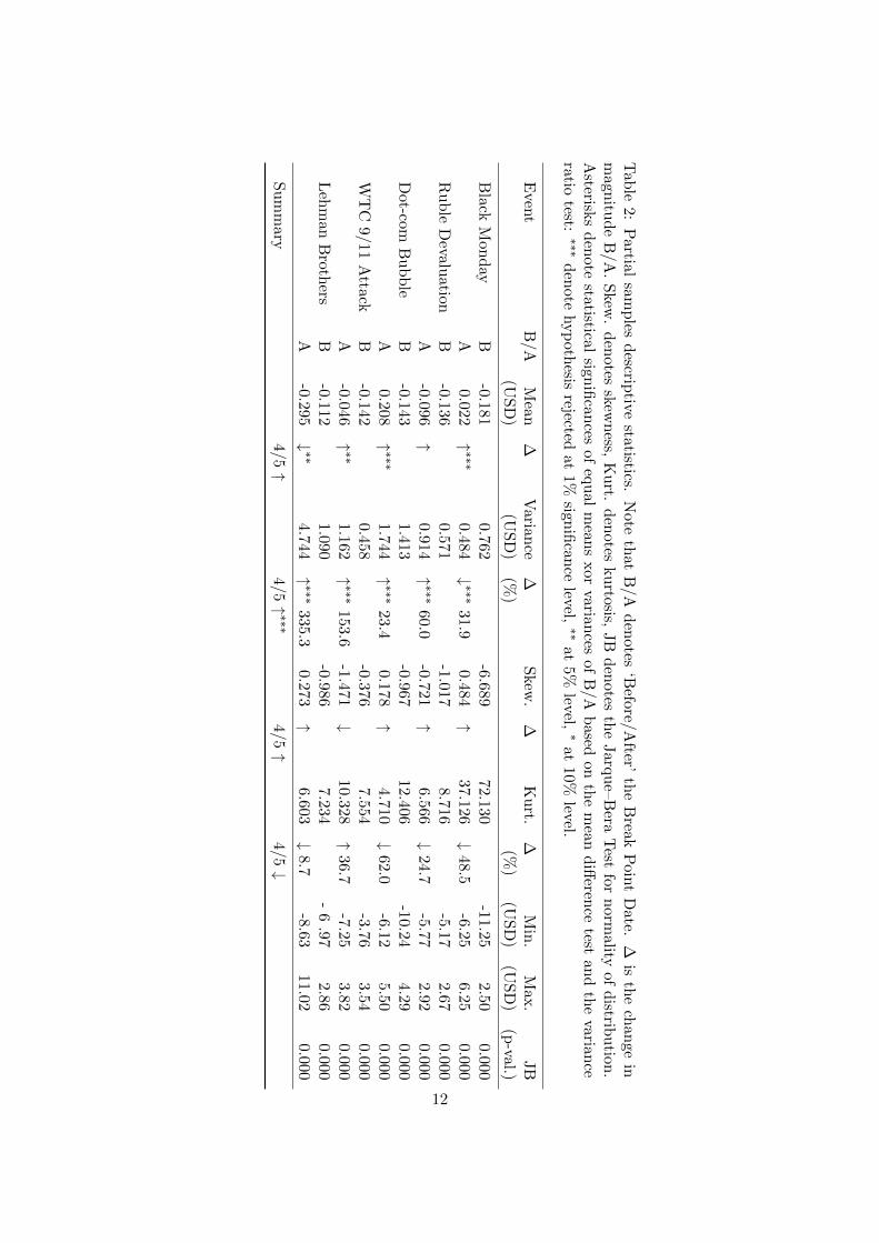
Figure 1 depicts probability density functions of the empirical distributions of the price differ-ences for each partial sample before and after the BPD. Excess kurtosis and heavy tails are distinctat first glance. Figure 2 shows tails of the empirical distributions of the price differences for eachpartial sample before and after the BPD. Table 2 then offers a summary of important descriptivestatistics keeping the same logic as Figure 1 and Figure 2.

5If a company changed its name, it usually keeps its ticker symbol and the historical data remain available.

11

Tab

le2:

Partial

samp

lesd

escriptive

statistics.N

oteth

atB

/Ad

enotes

‘Before/A

fter’th

eB

reakP

oint

Date.

∆is

the

chan

gein

magn

itud

eB

/A

.S

kew.

den

otesskew

ness,

Ku

rt.d

enotes

ku

rtosis,JB

den

otesth

eJarq

ue–B

eraT

estfor

norm

alityof

distrib

ution

.A

sterisks

den

ote

statistical

signifi

cances

ofeq

ual

mean

sxor

variances

ofB

/Ab

asedon

the

mean

diff

erence

testan

dth

evarian

ceratio

test:∗∗∗

den

ote

hyp

oth

esisrejected

at1%

signifi

cance

level,∗∗

at5%

level,∗

at10%

level.

Even

tB

/AM

ean

∆V

ariance

∆Skew

.∆

Ku

rt.∆

Min

.M

ax.

JB

(US

D)

(USD

)(%

)(%

)(U

SD

)(U

SD

)(p

-val.)

Black

Mon

day

B-0

.181

0.762-6.689

72.130-11.25

2.500.000

A0.0

22↑ ∗∗∗

0.484↓ ∗∗∗

31.90.484

↑37.126

↓48.5

-6.256.25

0.000R

ub

leD

evaluatio

nB

-0.1360.571

-1.0178.716

-5.172.67

0.000A

-0.0

96↑

0.914↑ ∗∗∗

60.0-0.721

↑6.566

↓24.7

-5.772.92

0.000D

ot-com

Bu

bb

leB

-0.143

1.413-0.967

12.406-10.24

4.290.000

A0.2

08↑ ∗∗∗

1.744↑ ∗∗∗

23.40.178

↑4.710

↓62.0

-6.125.50

0.000W

TC

9/11

Attack

B-0

.142

0.458-0.376

7.554-3.76

3.540.000

A-0

.046

↑ ∗∗1.162

↑ ∗∗∗153.6

-1.471↓

10.328↑

36.7-7.25

3.820.000

Leh

man

Broth

ersB

-0.112

1.090-0.986

7.234-

6.97

2.860.000

A-0.29

5↓ ∗∗

4.744↑ ∗∗∗

335.30.273

↑6.603

↓8.7

-8.6311.02

0.000

Su

mm

ary

4/5

↑4/5

↑ ∗∗∗4/5

↑4/5

↓

12

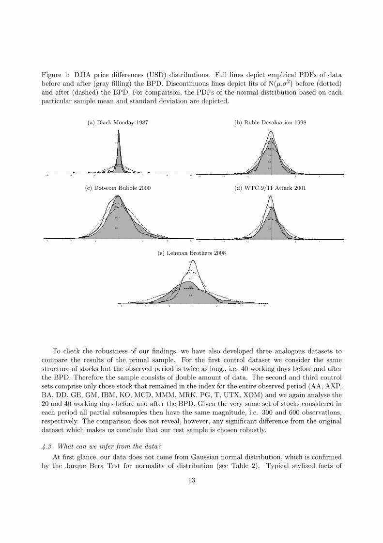
Figure 1: DJIA price differences (USD) distributions. Full lines depict empirical PDFs of databefore and after (gray filling) the BPD. Discontinuous lines depict fits of N(µ,σ2) before (dotted)and after (dashed) the BPD. For comparison, the PDFs of the normal distribution based on eachparticular sample mean and standard deviation are depicted.

(a) Black Monday 1987

-6 -4 -2 2 4 6

0.5

1.0

1.5

2.0

2.5

(b) Ruble Devaluation 1998

-6 -4 -2 2 4 6

0.1

0.2

0.3

0.4

0.5

0.6

0.7

(c) Dot-com Bubble 2000

-6 -4 -2 2 4 6

0.1

0.2

0.3

0.4

(d) WTC 9/11 Attack 2001

-6 -4 -2 2 4 6

0.2

0.4

0.6

0.8

(e) Lehman Brothers 2008

-6 -4 -2 2 4 6

0.1

0.2

0.3

0.4

0.5

To check the robustness of our findings, we have also developed three analogous datasets tocompare the results of the primal sample. For the first control dataset we consider the samestructure of stocks but the observed period is twice as long., i.e. 40 working days before and afterthe BPD. Therefore the sample consists of double amount of data. The second and third controlsets comprise only those stock that remained in the index for the entire observed period (AA, AXP,BA, DD, GE, GM, IBM, KO, MCD, MMM, MRK, PG, T, UTX, XOM) and we again analyse the20 and 40 working days before and after the BPD. Given the very same set of stocks considered ineach period all partial subsamples then have the same magnitude, i.e. 300 and 600 observations,respectively. The comparison does not reveal, however, any significant difference from the originaldataset which makes us conclude that our test sample is chosen robustly.

4.3. What can we infer from the data?

At first glance, our data does not come from Gaussian normal distribution, which is confirmedby the Jarque–Bera Test for normality of distribution (see Table 2). Typical stylized facts of

13

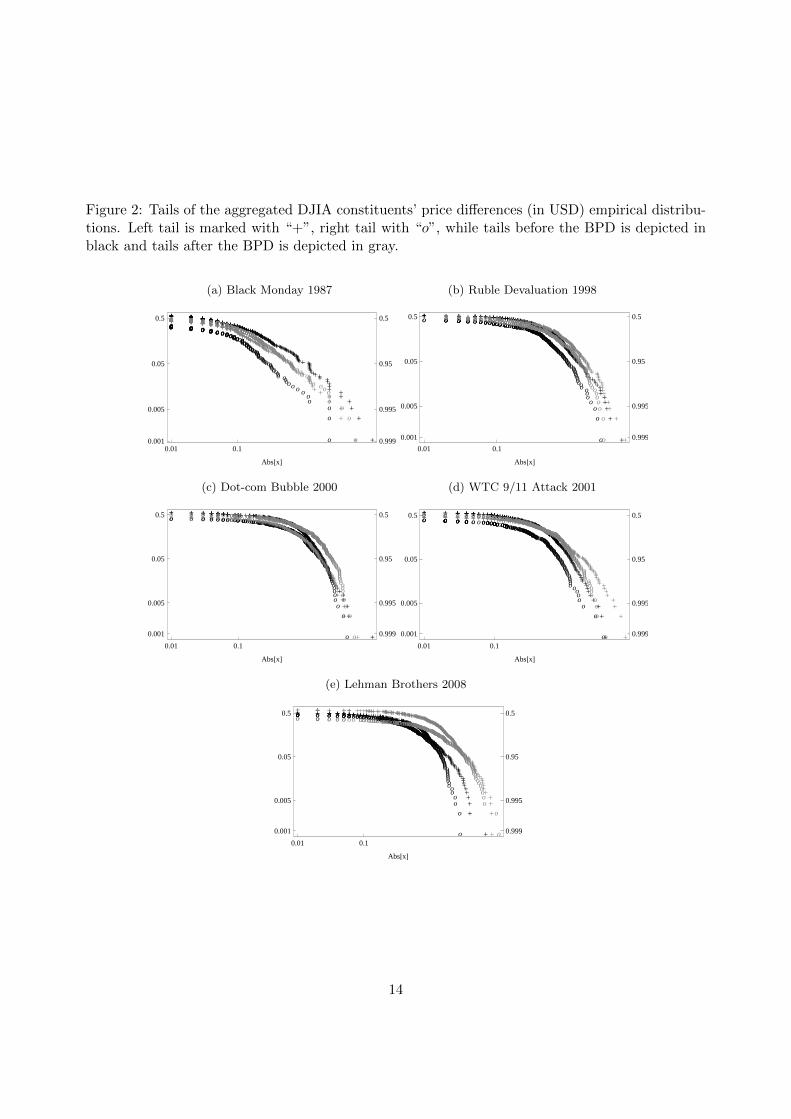
Figure 2: Tails of the aggregated DJIA constituents’ price differences (in USD) empirical distribu-tions. Left tail is marked with “+”, right tail with “o”, while tails before the BPD is depicted inblack and tails after the BPD is depicted in gray.

(a) Black Monday 1987

+

+

+

+

++

+++

++++

++++++++++++++++

+++++++

+++++++++

+++++++++++

++++++++++++++

++++++++++++++++

+++++++++++++++++++

+++++++++++++++++++++++

+++++++++++++++++++++++++++++++++++++++++++++++++++++++++++++++++++++++++++++++++++++++++++++++++++++++++++++++++++++++++++++++++++++++++++++

ooooooooooooooo oooooooooooo ooooooo oooooooooo oooooo oooooooooooooooooooooooooooooooooooooooooooooooooooooooooooooooooooooooooooooooooooooooooooooooooooo ooooo o o oo

oo

o +

+

+

+

++

+++

+++++++

++++

++++++

+++++++++

+++++++++++++

+++++++++++

++++++++++++++

+++++++++++++++++

++++++++++++++++++++++++++++++++++++++++++++++++++++++++++++++++++++++++++++++++++++++++++++++++++++++++++++++++++++

oooooooooo oooooooooooo ooooooo oooooooo oooooooooooo oooooooooooooooooooooooooooooooooooooooooooooooooooooooooooooooooooooooooooooooooooooooooooooooooooooooooooooooooooooooooooooooooooooooooooooooooooooooooooooooooooooo ooooo ooooo

oo

o0.01 0.1

0.5

0.05

0.005

0.001

0.5

0.95

0.995

0.999

Abs@xD

(b) Ruble Devaluation 1998

+

+

+

+

++++

++++

+++++

+++++

++++++

+++++++

+++++++++

+++++++++++

+++++++++++++++++++++++++++++

+++++++++++++++++++

+++++++++++++++++++++++

+++++++++++++++++++++++++++++

+++++++++++++++++++++++++++++++++++

++++++++++++++++++++++++++++++++++++++++++

++++++++++++++++++++++++++++++++++++++++++++++++++++++++++++++++++++++++

oo oooo oooooo ooooo ooo oooo oooooooooooooooooooooooooooooooooooooooooooooooooooooooooooooooooooooooooooooooooooooooooooooooooooooooooooooooooooooooooooooooooooooooooooooooooooooooooooooooooooooooooooooooooooooooooooooooooooooooooooooooooo oooooo

o +

+

+

+

++++++

++++++

+++++++++++++

++++++++

+++++++++

+++++++++++

+++++++++++++

+++++++++++++++++

+++++++++++++++++++++

+++++++++++++++++++++++++

++++++++++++++++++++++++++++++

+++++++++++++++++++++++++++++++++++++++++++++++++++++++++++

++++++++++++++++++++++++++++++++++++++++++++++++++++++++++++++++++ooo ooooo oooooo oooooo ooo oooooooooooooooooooooooooooooooooooooooooooooooooooooooooooooooooooooooooooooooooooooooooooooooooooooooooooooooooooooooooooooooooooooooooooooooooooooooooooooooooooooooooooooooooooooooooooooooooooooooooooooooooooooooooooooooooooooooooooooooo

o0.01 0.1

0.5

0.05

0.005

0.001

0.5

0.95

0.995

0.999

Abs@xD

(c) Dot-com Bubble 2000

+

+

+

+

++

++

++++++++

++++

+++++++++++++

+++++++++++++

++++++++++++++++++

+++++++++++++++

+++++++++++++++++++

+++++++++++++++++++++++

++++++++++++++++++++++++++++

++++++++++++++++++++++++++++++++++

++++++++++++++++++++++++++++++++++++++++++

++++++++++++++++++++++++++++++++++++++++++++++++++++++++++++++++++++++++++++++++++++++++++++++++++++++++++

oo o oo oo oo oooooooooooo oooooooooooooooooooooooooooooooooooooooooooooooooooooooooooooooooooooooooooooooooooooooooooooooooooooooooooooooooooooooooooooooooooooooooooooooooooooooooooooooooooooooooooooooooooooooooooooooooooooooooooooooooooooooooo

o

o +

+

+

+

++++++++

++++

+++++++

++++++

++++++++++++

++++++++++

++++++++++++++++++++

+++++++++++++++++

+++++++++++++++++++++

+++++++++++++++++++++++++

+++++++++++++++++++++++++++++++

++++++++++++++++++++++++++++++++++++++

++++++++++++++++++++++++++++++++++++++++++++++++++++++++++++++++

o oo oo oo oooo oooooooooooooooo ooooo ooooooooooooooooooooooooooooooooooooooooooooooooooooooooooooooooooooooooooooooooooooooooooooooooooooooooooooooooooooooooooooooooooooooooooooooooooooooooooooooooooooooooooooooooooooooooooooooooooooooooooooooooooooooooooooooooooooooooooooooooooooooooooooooooooooooooooo

o

o0.01 0.1

0.5

0.05

0.005

0.001

0.5

0.95

0.995

0.999

Abs@xD

(d) WTC 9/11 Attack 2001

+

+

+

+

+++++

+++

++++

++++++++++

+++++++

++++++++

++++++++++

+++++++++++++

++++++++++++++++++++++++

+++++++++++++++++++++

+++++++++++++++++++++++++

+++++++++++++++++++++++++++++++

++++++++++++++++++++++++++++++++++++++

++++++++++++++++++++++++++++++++++++++++++++++

+++++++++++++++++++++++++++++++++++++++++++++++++++++++++++++++++++++++++++++++++++++++++++

ooo ooooooooo ooooo oooooo oo ooooooooooooooooooooooooooooooooooooooooooooooooooooooooooooooooooooooooooooooooooooooooooooooooooooooooooooooooooooooooooooooooooooooooooooooooooooooooooooooooooooooooooooooooooooooooooooooooooooooooooooo

o

o +

+

+

+

++

++

++++

++++

+++++++

++++++

++++++++

++++++++++++++

+++++++++++++

+++++++++++++++

+++++++++++++++++++

+++++++++++++++++++++++

++++++++++++++++++++++++++++

++++++++++++++++++++++++++++++++++

++++++++++++++++++++++++++++++++++++++++++++++++++++++++++++++++++++++++++++++++++++++++

oooo ooooooo oo oooo ooo oooooooooooooooooooooooooooooooooooooooooooooooooooooooooooooooooooooooooooooooooooooooooooooooooooooooooooooooooooooooooooooooooooooooooooooooooooooooooooooooooooooooooooooooooooooooooooooooooooooooooooooooooooooooooooooooooooooooooooooooooooooooooooooooooooooooooooooooooooooooooooo

o0.01 0.1

0.5

0.05

0.005

0.001

0.5

0.95

0.995

0.999

Abs@xD

(e) Lehman Brothers 2008

+

+

+

+++

+++++

++++++

+++++

+++++++++++++

+++++++++

+++++++++++

+++++++++++++

++++++++++++++++++++++++++++++++++++++

+++++++++++++++++++++++++

++++++++++++++++++++++++++++++

++++++++++++++++++++++++++++++++++++++

++++++++++++++++++++++++++++++++++++++++++++++++++

+++++++++++++++++++++++++++++++++++++++++++++++++++++ooooo oo ooo ooo oooo oooooooooooooooooooooooooooooooooooooooooooooooooooooooooooooooooooooooooooooooooooooooooooooooooooooooooooooooooooooooooooooooooooooooooooooooooooooooooooooooooooooooooooooooooooooooooooooooooooooooooooooooooooooooooooooooooooooooooooooooooooooooooooooo

o

o +

+

+

++

++++++

++++++++

++++++

+++++++++

++++++++++++++

+++++++++++++++++++++++++++

++++++++++++++++++

++++++++++++++++++++++++++++++++++

+++++++++++++++++++++++++++++

++++++++++++++++++++++++++++++++++++

++++++++++++++++++++++++++++++++++++++++++++

++++++++++++++++++++++++++++++++++++++++++++++++++++++

++++++++++++++++++++++++++++++++++++++++++++++++++++++++++++++++

oo ooooo oo oo oo oo ooooooooooooooooooooooooooooooooooooooooooooooooooooooooooooooooooooooooooooooooooooooooooooooooooooooooooooooooooooooooooooooooooooooooooooooooooooooooooooooooooooooooooooooooooooooooooooooooooooooooooooooo

o

o0.01 0.1

0.5

0.05

0.005

0.001

0.5

0.95

0.995

0.999

Abs@xD

14

financial returns such as excess kurtosis or heavy tails are also fulfilled. In Table 2 one can clearlysee shifts of mean, variance, skewness and kurtosis between the ‘before’ and ‘after’ periods. Thefirst three of these four descriptive statistics increase in four of five analysed periods, while kurtosisdecreases in the same ratio of cases. These findings are not only interesting from the statisticalpoint of view, economic interpretation might be interesting to study as well.

Let us start with mean which rather increases. One of the possible explanations might bethat after a sudden market crash the resulting short-run tendency is to compensate the huge dropin prices by several increases. Speculators might play a substantial role in this situation. Theseincreases then statistically exceed the huge drop at the beginning which leads to the overall pictureof a higher mean. Another rationale might be that the market crash is a climax when the negativetrend of market prices culminates. After that, therefore, there is no more space for drops and themarket naturally increases.

Increasing variance measures the increasing market risk and uncertainty resulting in its unpre-dictability. This is one of the accompaniments of all turbulent market periods.

The most challenging issue for an economic interpretation is the increasing skewness. Thismeans that the mass of the distribution shifts from right to left, the right tail becomes longerand high values become more scarce. All of these features are likely to be related to general crisistendencies but their interpretation with regard to the increasing mean does not seem unambiguous.

Finally, for the decreasing trend of kurtosis several straightforward explanations may apply. Inthe crisis period after a market crash extreme observations (both negative and positive) becomemore likely and, in the contrary, observations close to mean are less probable. Tails of relateddistribution thus become heavier as shown by Figure 1 and Figure 2 and kurtosis decreases.

The most interesting part now will be to compare these considerable empirical results with theoutcomes of the model simulations.

5. A setup for simulations

To be able to mutually compare all different model setups, we define a joint setup which willbe used for all simulations. In the simulations, we follow our previous work (Barunik et al., 2009;Vacha et al., 2009, 2012) basing our model in the Brock and Hommes (1998) setting. Adaptivebelief system is compactly described (Hommes, 2006) by the three mutually dependent equations:

Rxt =H∑

h=1

nh,tfh,t + εt ≡H∑

h=1

nh,t(ghxt−1 + bh) + εt, (18)

nh,t =exp(βUh,t−1)∑Hh=1 exp(βUh,t−1)

, (19)

Uh,t−1 = (xt−1 −Rxt−2)fh,t−2 −Rxt−2

aσ2

≡ (xt−1 −Rxt−2)ghxt−3 + bh −Rxt−2

aσ2, (20)

where εt denotes the noise term representing the market uncertainty and unpredictable occasions.The Walrasian price formation mechanism is inherently comprised within the first Equation 18 ofthis system as described in detail in section 3 and summarized in Equation 13 and Equation 14.

The inevitable feature of all heterogeneous agent models are too many degrees of freedomtogether with a large number of parameters which can be modified and studied. Therefore we need

15

to fix several variables to be able to analyse particular changes of the model ceteris paribus. As inBarunik et al. (2009) and Vacha et al. (2009), we set the constant gross interest rate R = 1+r = 1.1;the linear term 1/aσ2 consisting of the risk aversion coefficient a > 0 and the constant conditionalvariance of excess returns σ2 is fixed to 1. In addition to that, we use relatively small number oftraders, H = 5 and neither memory nor learning process are implemented to keep the impact ofthe behavioural modifications as clear as possible.

To examine the impact of suggested changes on the model outcomes, we rely on Monte Carlomethods. To obtain statistically valid and reasonably robust sample, we rely on the number of 100runs. The trend parameter gh is drawn from the normal distribution N(0, 0.16), the bias parameterbh is drawn from the normal distributionN(0, 0.09). When g1 = b1 = 0, fundamentalists are presentat the market. We allow fundamentalists to appear in the market either randomly or by control.

Finally, the magnitude of noise has to be considered carefully as it represents the notion ofmarket uncertainty so it is inevitable part of the model, but it should not overshadow the effect ofanalysed modifications. We examine the effect of various noise settings, namely εt ∈ U(−0.02, 0.02),εt ∈ U(−0.05, 0.05) and εt ∈ U(−0.1, 0.1) and conclude that although different noise variancecauses some minor changes in model outcomes, all models across different noises embody majorsimilarities. Thus the noise term εt is drawn from the uniform distr. U(−0.05, 0.05) which seemreasonable6 to us.

In our simulations, we change the intensity of choice β and the intensity of the behaviouralelement. The literature estimating β using a real marked data is extremely scarce as it is difficultto estimate the intensity of choice due to the non-linear nature of the model. One recent exampleis Frijns et al. (2010, pg. 2281) who find that the intensity of choice “is positive and of considerablemagnitude throughout the sample” of daily closing DAX prices covering the entire year 2000. Henceβ still remains a rather theoretical concept. However, larger β implies higher willingness of tradersto switch between strategies based on their profitability — the best strategies at each specificperiod are chosen by more agents — and reversals in the price development are thus more likely.To comprise the large variety of possible values we use7 the range β ∈ 〈5, . . . 500〉 with single stepsof 55, i.e. β = {5, 60, 115, 170, 225, 280, 335, 390, 445, 500}. On the other hand, for each behaviouralelement the range varies and we describe its logic in further sections. The length of the generatedtime series corresponds to 250 days, i.e. t = {0, . . . 250}. First 10% of observations are discardedas initial period.

The way we implement the behavioural elements into the framework is that we change thedynamics of the model in the middle of generated time series, i.e. from the 126th iteration viainjecting a new behavioural element. Then, we study the dynamics of the system closely beforeand after this change. The choice of the empirical benchmark sample introduced in the previoustext reflects exactly this procedure. The last 10% of observations are discarded as well to obtainsamples of the same magnitude.

In studying the effect of behavioural elements on the model outcomes, we focus on four sub-series. First, we split the generated series into 2 halves, before and after the 126 iteration whenbehavioural break is put into the model. Second, we focus on last 20 observations before thebehavioural break and first 20 observations after the behavioural break. By cumulating these four

6Results for different noise settings are available upon request from authors.7In the choice of β, we follow our previous research. In Barunik et al. (2009) and Vacha et al. (2009), we use

β = 300, in Vacha et al. (2012), we use β = 500 for example. Results for different β ∈ 〈0, . . . 1000〉 are available uponrequest from authors.

16

groups of series from different iterations, we are finally left with (i) the complete ‘before’ sampleof 10000 observations; (ii) the 20 day ‘before’ sample of 2000 observations; (iii) the 20 day ‘after’sample of 2000 observations; (iv) the complete ‘after’ sample of 10000 observations.

5.1. Modelling of behavioural patterns: herding

As a certain notion of herding is naturally included8 in the evolutionary adaptive system ofstrategy switching, we present different original modelling approach to herding. The examinationof herding patterns in HAM is always based on short-run profitabilities of individual strategies andherding is detected via the evolution of market fractions nh,t. This concept of herding is hencemore or less (boundedly) rational. Therefore we introduce a concept of rather irrational, ‘blind’herding, which is based on public information and aims to imitate traders’ behaviour during largestocks sell-offs after a market crash.

In this approach one of trading strategies (h = 5) does not behave in the traditional way butcopies the behaviour of the most successful traders of the previous day. At time t the strategyprimarily evaluates its own performance measure, then compares the performance measures of allother strategies and for the next period t + 1 it adjusts its beliefs about the trend g5 and bias b5parameters, so that they mimic the last period’s most profitable strategy. The mimicking effect isthus one period lagged and this delay represents the reaction of less informed market participantwho just follow the crowd.

Thus instead of 5 strategies present at the market, we can observe only 4 of them while thelast, fifth mimics the most profitable one. Including the fifth mimicking strategy can lead tosubstantially different results in favor of the strategy which is currently being imitated, especiallywhen the intensity of choice β is small.

5.2. Modelling of behavioural patterns: overconfidence

Behavioural overconfidence can be modelled as a routine tendency to overestimate the accuracyof own judgments. Trying to incorporate this into the model framework, we are left with noother choice than work with the trend gh and bias bh parameters. However, this makes perfectsense and we model overconfidence as an overestimation of generated values. Roughly speaking,an overconfident trend chasing trader behaves even more surely and follows the observed trendstrongly than in a normal (randomly generated) situation. He also expects the price to rise or dropeven more than according to his (randomly generated) premises. The range of the ‘overconfidenceelement’ is 〈0.05, . . . 0.5〉 and one can imagine this as the representation of the excess assurancein percentage terms — from 5 to 50%. Three options are examined: overconfidence affecting thetrend parameter gh only, overconfidence affecting the bias parameter bh only, and overconfidenceaffecting both parameters. As overconfidence is positive ‘from definition’, negative values are notconsidered.

5.3. Modelling of behavioural patterns: market sentiment

We model the market sentiment as shifts of the mean values of probability distributions fromwhich the trend parameter gh and the bias parameter bh are generated. Both impacts of the ‘posi-tive’ and the ‘negative’ sentiment are examined. Vacha et al. (2009) model the market sentiment asjumps of the trend parameter gh between realizations from the normal distributions N(0.04, 0.16)

8See e.g. Chiarella and He (2002b), Chiarella et al. (2003), De Grauwe and Grimaldi (2006), or Hommes (2006).

17

and N(−0.04, 0.16). We generally consider four options: (i) sentiment affecting the trend param-eter gh only (the same case as we consider in Vacha et al., 2009); (ii) sentiment affecting the biasparameter bh only; (iii) sentiment affecting both parameters; (iv) and finally so called ‘mixed’ casewhere the positive sentiment affecting bias bh is combined with the negative sign of the trendparameter gh and vice versa. The interpretation of both effects is, however, considerably different.

If we decrease the mean of the trend parameter gh, the contrarian strategies are more likelyto be generated. Nonetheless, this does not tell much about the type of sentiment we have set —whether the sentiment is intended to be positive or negative — we primarily adjust the responseof agents to actual price development. On the other hand, manipulating with the mean of thebias parameter bh we directly set the trend — decreasing the mean we model negative marketsentiment (price rather drops tomorrow) and vice versa. Next, as we aim to model the behaviourin extremely turbulent times, we assume higher shifts than only one tenth of the standard deviationas in Vacha et al. (2009). The range for the positive sentiment element is 〈0.04, . . . , 0.4〉 for trendand 〈0.03, . . . , 0.3〉 for bias, i.e. the minimum is one tenth of the standard deviation and themaximum equals one standard deviation of related distributions. For degree of negative sentiment,the opposite values 〈−0.4, . . . ,−0.04〉 for trend and 〈−0.3, . . . ,−0.03〉 for bias are used. At firstsight, this approach might seem a little similar to the overconfidence modelling, but the oppositeis true. Although both appertain to the trend and bias parameters, in the overconfidence case weonly symmetrically strengthen traders’ responses to the current market development, while in themarket sentiment case we asymmetrically deflect the market behaviour and traders’ beliefs.

5.4. Illustration of generated series

To illustrate the impact of the behavioural elements incorporation on the model outcomes,Figure 3 depicts three pairs of randomly generated series — one for herding, one for overconfidenceaffecting both parameters, and one for market sentiment affecting both parameters. One canclearly see the structural change at the BPD. Regarding the single series properties, these arestrongly influenced by the random combination of generated parameters and we use it here justas an illustration. However, aggregated distribution resulting from all simulations in total indeedexhibits properties which are in agreement with empirical data in financial markets.

6. Results and interpretations

In total, we simulate 13 different setup combinations including no behavioural impact, herding,three different setup combinations for overconfidence, and eight setup combinations for marketsentiment according to the description in previous text. The overview of the aggregate results issummarised in Table 3.

Within each simulation, we keep tracking many features. First, we evaluate the same patternwhich has been revealed within the empirical benchmark sample, i.e. the shifts of mean, variance,skewness, and kurtosis between the ‘before’ and ‘after’ periods. While studying the empirical data,we have found that the first three of these four descriptive statistics increase in four of five analysedperiods, while kurtosis decreases in the same ratio of cases. We also mention the arithmetic averageof the percentual magnitude changes before and after the BPD for variance and kurtosis.

Second, using the Cramer–von Mises Test for equal distributions we observe whether there arestatistically significant differences among particular samples, namely we compare: the complete‘before’ sample (B) to the ‘20 day before’ sample (b), the ‘20 day before’ sample (b) to the ‘20 dayafter’ sample (a), the ‘20 day after’ sample (a) to the complete ‘after’ sample (A), and finally the

18

Tab

le3:

Sim

ula

tion

sR

esu

lts

—O

verv

iew

.N

ote

that

Var

.d

enot

esva

rian

ce,

Ske

w.

den

otes

skew

nes

s,K

urt

.d

enot

esku

rtos

is,

+/-

den

ote

‘pos

itiv

e/n

egat

ive’

mar

ket

senti

men

t.B

/Ad

enot

es‘B

efor

e/A

fter

’th

eB

reak

Poi

nt

Dat

e.C

aps

stan

dfo

rth

eco

mp

lete

sam

ple

s,sm

all

lett

ers

for

the

20

day

ssa

mp

les.

∅∆

isth

ear

ith

met

icav

erag

eof

%m

agn

itu

de

chan

ges

B/A

the

Bre

akP

oint

Dat

efo

rva

rian

cean

dku

rtos

is.

Inth

eC

ram

er–vo

nM

ises

Tes

tfo

req

ual

dis

trib

uti

ons

B/A

(H0)

the

nu

mb

erof

non

-rej

ecti

ons

at5%

sig.

leve

lis

cou

nte

d.

Inth

eJarq

ue–

Ber

aT

est

for

nor

mal

ity

ofd

istr

ibu

tion

(H0)

nu

mb

erof

non

-rej

ecti

ons

at5%

sign

if.

leve

lis

cou

nte

d.

Sam

ple

Mea

n↑

Var.

↑∅

∆S

kew

.↑

Ku

rt.

↓∅

∆C

ram

er–v

onM

ises

T.

Jar

qu

e–B

era

T.

(ou

tof

100

run

s)(%

)(o

ut

of10

0ru

ns)

(%)

B-b

b-a

a-A

A-B

Bb

aA

No

Beh

avio

ura

lIm

pac

t48

53

9.3

5048

18.5

100

100

100

100

27

72

Her

din

g78

39

24.0

6044

44.0

100

6110

04

11

31

Ove

rcon

fid

ence

(bia

s)47

9781

.851

5441

.710

018

100

21

47

0O

verc

onfi

den

ce(t

ren

d)

52

9414

5.9

488

557.

110

098

100

581

70

0O

verc

onfi

den

ce53

9954

8.7

534

695.

510

014

100

14

131

0M

.S

enti

men

t+(b

ias)

100

7933

.696

3620

9.9

100

310

00

18

52

M.

Sen

tim

ent+

(tre

nd

)47

9925

1.9

479

641.

710

046

100

171

162

0M

.S

enti

men

t+(m

ix)

100

3-2

0.0

5174

-20.

710

01

100

01

616

4M

.S

enti

men

t+10

099

443.

386

1074

0.4

100

410

00

37

00

M.

Sen

tim

ent-

(bia

s)2

7532

.910

4056

100

310

00

16

60

M.

Sen

tim

ent-

(tre

nd

)44

2-2

5.5

4686

-24.

510

070

100

222

318

5M

.S

enti

men

t-(m

ix)

097

429.

118

1371

3.4

100

110

00

29

22

M.

Sen

tim

ent-

02

-21.

632

78-2

0.7

100

310

00

13

103

19

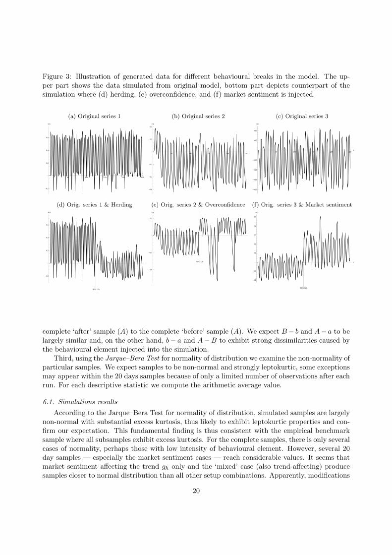
Figure 3: Illustration of generated data for different behavioural breaks in the model. The up-per part shows the data simulated from original model, bottom part depicts counterpart of thesimulation where (d) herding, (e) overconfidence, and (f) market sentiment is injected.

(a) Original series 1

50 100 150 200 250t

-0.2

0.2

0.4

0.6

xHtL

(b) Original series 2

50 100 150 200 250t

-0.6

-0.4

-0.2

0.2

0.4

xHtL

(c) Original series 3

50 100 150 200 250t

-0.20

-0.15

-0.10

-0.05

0.05

0.10

xHtL

(d) Orig. series 1 & Herding

BPD 126

t

-0.2

0.2

0.4

0.6

xHtL

(e) Orig. series 2 & Overconfidence

BPD 126

t

-1.0

-0.5

0.5

xHtL

(f) Orig. series 3 & Market sentiment

BPD 126

t

-0.2

-0.1

0.1

0.2

0.3

0.4

0.5

xHtL

complete ‘after’ sample (A) to the complete ‘before’ sample (A). We expect B− b and A− a to belargely similar and, on the other hand, b− a and A−B to exhibit strong dissimilarities caused bythe behavioural element injected into the simulation.

Third, using the Jarque–Bera Test for normality of distribution we examine the non-normality ofparticular samples. We expect samples to be non-normal and strongly leptokurtic, some exceptionsmay appear within the 20 days samples because of only a limited number of observations after eachrun. For each descriptive statistic we compute the arithmetic average value.

6.1. Simulations results

According to the Jarque–Bera Test for normality of distribution, simulated samples are largelynon-normal with substantial excess kurtosis, thus likely to exhibit leptokurtic properties and con-firm our expectation. This fundamental finding is thus consistent with the empirical benchmarksample where all subsamples exhibit excess kurtosis. For the complete samples, there is only severalcases of normality, perhaps those with low intensity of behavioural element. However, several 20day samples — especially the market sentiment cases — reach considerable values. It seems thatmarket sentiment affecting the trend gh only and the ‘mixed’ case (also trend-affecting) producesamples closer to normal distribution than all other setup combinations. Apparently, modifications

20

affecting trend gh when the behavioural ‘sentiment element’ is included have certain tendency tooffset the ability to produce real market-like leptokurtic distributions — one of the most highlightedfeatures of the model. This finding is, however, partially consistent with the benchmark sampletendency to exhibit decreases in kurtosis after the BPD.

6.2. Empirical pattern fitting

Let us look on results of the three behavioural modifications of the model. Herding seems toaffect the model structure the least. It exhibits more or less an average effect on all descriptivestatistics with prevailing effect of kurtosis increase which goes counter the empirical findings.Although the presence of the herding towards the most profitable strategy produces some minordifferences, namely mean shifts and dissimilarities in distributions, herding effect is comparativelyrather similar to the case without any behavioural impact. When comparing the distributions ofthe data 20 days before and after the herding occurs in the model (b − a case) we can see thatdistribution does not change significantly in 61 out of 100 cases.

While herding does not bring any strong results, overconfidence seems to influence the modelmuch more significantly. All three overconfidence setups increase variance in the large majority ofcases (94 to 99 out of 100). This result is comparable with our empirical findings as well as withconclusions of Daniel et al. (1998) and in fact is expected. On the other hand, overconfidence doesnot affect the mean of the distributions. An intriguing feature is the rapid variance and kurtosisincrease after the BPD in both cases with the trend overconfidence. When comparing these resultsto the findings from the empirical data we can see that overconfidence affecting the bias parameterbh only reveals substantially higher ability to fit the decreasing kurtosis empirical pattern. At thesame time it does not produce such extensive variance and especially kurtosis increases. Whenthinking about an economic interpretation, one can understand this specific setup as a situationwhen all market participant strictly use similar pricing models and thus their trend extrapolationis not a subject to any bias, while their personal feelings and expectations of the market futuredevelopment are highly impacted by overconfidence. Moreover, only in 18 out of 100 cases we cannot distinguish between the distributions of generated data ’before’ and ’after’ the BPD. In thecase of overconfidence affecting trend parameter, 98 out of 100 cases can not be distinguished fromeach other. This means that overconfidence affecting trend does not change the distribution ofgenerated data at all. Thus we conclude that the case of overconfidence affecting bias matches theempirical data best.

Turning our attention to the market sentiment we find out that it seems to be — comparedto the previous modifications — the most promising behavioural change of the model structure.At first glance, effects of the positive and the negative market sentiment generate roughly inverseresults. The positive market sentiment fits the empirical benchmark sample pattern considerablybetter, whereas the negative market sentiment is able only to mimic decreases in kurtosis (2 of 4cases) and variance increases (2 of 4 cases). This might be explained in a similar way as we offerfor the positive mean shifts within the empirical benchmark sample.

As the positive sentiment matches the behaviour found in the empirical data best, we focuson its results mainly. Market sentiment affecting trend gh seems to be a weak modification asit exhibits average values for the mean and skewness shifts and has very low performance in thecase of kurtosis. Mixed sentiment cancels the important variance shift almost entirely out but isable to mimic the kurtosis decrease. Again, we observe excessive variance and especially kurtosisupward jumps when the trend affecting sentiment is introduced. Sentiment changes affectingeither both trend gh and bias bh or bias bh only seem to be the most successful modifications

21

and we again conclude that the market sentiment affecting bias parameter bh only best matchesthe empirical findings. This particular modification embodies higher performance in the kurtosisdecrease fitting and, most importantly, it exhibits much more reasonable percentual changes ofvariance and kurtosis in comparison with the empirical values.

Employing the Cramer–von Mises Test for equal distributions we study the ability of particularbehavioural modifications to produce significantly different data distributions before and after theBPD. From this perspective, herding and all trend affecting setup combinations generally seemto be the weakest modifications. On the other hand, almost all non-trend sentiment modificationexhibit excellent results from this point of view. Our expectation that the 20 day samples and thecomplete samples from the same period come from the same distribution has been 100% affirmedas no single deviation appeared.

Increases of variance seem to be the most robust results of the majority of the overconfidenceand market sentiment setup combinations. This finding confirms the conclusions of Daniel et al.(1998) and Diks and Weide (2005). The tendency of the minimum and maximum values then alsomore or less confirms our expectation of higher volatility after the BPD. Nonetheless, the minimumand maximum values are rather chance results as they only represent a single extreme value of all100 runs.

6.3. Model extensions

While being rather successful in replicating empirical findings by behavioural injections in theHAM model, we focus on further possibilities of model extensions in order to test robustness ofour results. In further analysis, we drop the setups with negative market sentiment as these arefar from the empirical data.

The overviews of the aggregate results are summarised in Table 4 & 5. The structure of thetracked information remains the same as in the previous analysis.

6.3.1. Fundamentalists by default

Fundamentalists play crucial role in the theoretical model framework. Until now, we alloweda fundamental strategy to be generated only within random setting, but next we would like tostudy the change of the market behaviour in case when the one fundamental strategy will surelybe present in the market. Therefore, we will always set g1 = b1 = 0 for one of strategies.

Looking at the results, fundamentalists’ default presence seems to have only a minor and non-systematic impact on the model outcomes. It affects mainly kurtosis and moves only two setupcombinations slightly closer to the empirical benchmark sample. The effect on kurtosis is alsoevident from the results of the Jarque–Bera Test which rejects normality in more cases than withinthe primary results.

In the overconfidence case, fundamentalists strongly decrease variance but only for the setupcombination where both trend gh and bias bh are affected. For the same setup kurtosis stronglyincreases in the ‘before’ sample and strongly decreases in the ‘after’ sample. In this specific casefundamentalists thus balance the kurtosis magnitudes before and after the BPD.

In the market sentiment case, we can also observe decreasing fundamentalists’ impact on kur-tosis, but only in the ‘mix’ case.

6.3.2. Stochastic formation of parameters

It is perhaps more realistic to assume that the levels of the market sentiment or overconfidenceas well as the tendency to switch between particular strategies vary both among traders and in

22

Tab

le4:

Exte

nsi

ons

resu

lts

I.—

over

vie

w.

Not

eth

atV

ar.

den

otes

vari

ance

,S

kew

.d

enot

essk

ewn

ess,

Ku

rt.

den

otes

ku

rtos

is,

+/-

den

ote

‘pos

itiv

e/n

egat

ive’

mar

ket

senti

men

t.B

/Ad

enot

es‘B

efor

e/A

fter

’th

eB

reak

Poi

nt

Dat

e.C

aps

stan

dfo

rth

eco

mp

lete

sam

ple

s,sm

all

lett

ers

for

the

20

day

ssa

mp

les.

∅∆

isth

ear

ith

met

icav

erag

eof

%m

agn

itu

de

chan

ges

B/A

the

Bre

akP

oint

Dat

efo

rva

rian

cean

dku

rtos

is.

Inth

eC

ram

er–vo

nM

ises

Tes

tfo

req

ual

dis

trib

uti

ons

B/A

(H0)

the

nu

mb

erof

non

-rej

ecti

ons

at5%

sig.

leve

lis

cou

nte

d.

Inth

eJarq

ue–

Ber

aT

est

for

nor

mal

ity

ofd

istr

ibu

tion

(H0)

nu

mb

erof

non

-rej

ecti

ons

at5%

sign

if.

leve

lis

cou

nte

d.

Exte

nsi

on&

Sam

ple

Mea

n↑

Var

.↑

∅∆

Ske

w.

↑K

urt

.↓

∅∆

Cra

mer

–von

Mis

esT

.Jar

qu

e–B

era

T.

(ou

tof

100

run

s)(%

)(o

ut

of10

0ru

ns)

(%)

B-b

b-a

a-A

A-B

Bb

aA

Fu

nd

am

enta

list

s:

Her

din

g76

2914

.073

3730

.210

038

100

10

10

0O

verc

onfi

den

ce(b

ias)

5199

86.3

4652

57.5

100

1910

04

16

50

Ove

rcon

fid

ence

(tre

nd

)45

9812

7.8

426

419.

810

099

100

702

92

1O

verc

onfi

den

ce52

9810

3.8

5366

50.1

100

2010

04

04

21

M.

Sen

tim

ent+

(bia

s)99

7832

.993

3210

7.4

100

310

00

23

32

M.

Sen

tim

ent+

(tre

nd

)56

9824

1.7

606

524.

710

049

100

210

90

0M

.S

enti

men

t+(m

ix)

100

2-2

7.8

6584

-27.

010

02

100

00

214

2M

.S

enti

men

t+10

098

394.

487

860

6.0

100

310

00

13

10

Sto

chas

tic

Par

am

eter

s:

Her

din

g80

36-5

.147

5056

.510

076

100

131

77

1O

verc

onfi

den

ce(b

ias)

4198

74.8

5251

27.2

100

010

00

26

51

Ove

rcon

fid

ence

(tre

nd

)50

9916

7.8

522

765.

810

010

010

054

311

00

Ove

rcon

fid

ence

58

100

317.

156

363

6.4

100

010

00

48

10

M.

Sen

tim

ent+

(bia

s)100

8620

.794

3761

.410

00

100

02

71

0M

.S

enti

men

t+(t

ren

d)

51

9931

6.0

541

957.

810

018

100

00

40

0M

.S

enti

men

t+(m

ix)

100

3-2

1.7

4489

-22.

810

00

100

00

624

5M

.S

enti

men

t+10

0100

356.

498

394

6.0

100

010

00

35

00

23

Tab

le5:

Exten

sion

sR

esults

II.—

Overv

iew.

Note

that

Var.

den

otesvarian

ce,S

kew.

den

otessk

ewn

ess,K

urt.

den

otesku

rtosis,+

/-d

enote

‘positive/

neg

ative’m

arketsen

timen

t.B

/Ad

enotes

‘Before/A

fter’th

eB

reakP

oint

Date.

Cap

sstan

dfor

the

comp

letesa

mp

les,sm

all

lettersfo

rth

e20

day

ssam

ples.

∅∆

isth

earith

metic

averageof

%m

agnitu

de

chan

gesB

/Ath

eB

reakP

oint

Date

forvarian

cean

dku

rtosis.In

the

Cram

er–von

Mises

Test

foreq

ual

distrib

ution

sB

/A(H

0 )th

enu

mb

erof

non

-rejections

at5%

sig.level

isco

unted

.In

the

Jarq

ue–B

eraT

estfo

rnorm

alityof

distrib

ution

(H0 )

nu

mb

erof

non

-rejections

at5%

signif.

levelis

counted

.

Exten

sion&

Sam

ple

Mea

n↑

Var.

↑∅

∆S

kew.

↑K

urt.

↓∅

∆C

ramer–von

Mises

T.

Jarq

ue–B

eraT

.(ou

tof

100

run

s)(%

)(ou

tof

100ru

ns)

(%)

B-b

b-a

a-AA

-BB

ba

A

Com

bin

ations:

Herd

.&

Over.

(bias)

88

4952.7

6233

137.9100

72100

83

84

1H

erd.

&S

ent.+

(bias)

9958

111.387

29156.2

1000

1000

18

10

Over.

(b.)

&S

ent.+

(b.)

100

97112.7

9131

80.895

1100

01

103

2H

.&

O.

(b.)

&S

.+(b

.)100

6658.6

8633

122.9100

0100

01

102

0

Mem

ory:

Herd

ing

85

6970.9

6543

60.197

3395

100

10

0O

verconfi

den

ce(b

ias)49

95135.2

4753

101.9100

1198

31

22

1O

verconfi

den

ce(tren

d)

4195

96.246

5028.7

9715

953

01

21

Overcon

fid

ence

51

99362.1

528

400.499

1696

30

11

0M

.S

entim

ent+

(bia

s)99

64122.2

7748

161.3100

237

00

42

0M

.S

entim

ent+

(trend

)55

95299.2

5918

345.3100

2596

100

01

0M

.S

entim

ent+

(mix

)100

4-30.1

6776

-15.799

134

00

20

0M

.S

entim

ent+

98

97489.5

8414

506.698

131

01

20

0

24

time. In an effort to reflect this sensible idea, we introduce the stochastic formation of the intensityof choice β as well as the behavioural element intensity. Both parameters are newly generatedrandomly for each simulation, which means we employ 10.000 different random combinations ofthese two model inputs for each setup combinations. Parameter ranges remain the same, i.e.:

• The intensity of choice β is drawn from the uniform distribution U(5, 500);

• The intensity of overconfidence is drawn from the uniform distribution U(0.05, 0.5);

• The intensity of the market sentiment is drawn from the uniform distribution U(0.04, 0.4) fortrend gh and from U(0.03, 0.3) for bias bh.

Table 4 reveals that stochastic formation of parameters does not bring any considerable differ-ence to model outcomes. In fact, this modification does not change the structure of the results, soour previous findings are robust to change of parameters in the model.

6.3.3. Combinations

Next, we consider the possible combinations of more behavioural modifications in the model andexamine whether combinations of impacts lead rather to a consolidation of results or to cancelingthe effects out. We combine four setups which best match the empirical findings. Hence, followingcombinations emerge:

• Herding & overconfidence affecting the bias parameter bh only;

• Herding & market sentiment affecting the bias parameter bh only;

• Overconfidence & market sentiment affecting the bias parameter bh only;

• Combination of all these three modifications.

Results of these simulations seem ambiguous and at first glance it is not clear which componentdominates. The combinations of various modifications lead more likely to canceling the effectsout than to a consolidation of results. Market sentiment seems to be the governing element, butits effect is comparatively smaller when it is combined with other modifications than when itworks alone. Herding follows and outperforms the impact of overconfidence. Compared with theprimary findings, no strong tendencies are apparent, new results are most often either the same orsomewhere ‘half-way’ between original results.

6.3.4. Memory

The effect of memory is undoubtedly one of the most interesting features which can be studiedwithin the heterogeneous agent modelling. The real-life parallel with the human memory and learn-ing is apparent. As Hommes (2006, pg. 56) points out, “another important issue is how memoryin the fitness measure affects stability of evolutionary adaptive systems and survival of technicaltrading”. Memory effect has been widely examined in various studies and we also incorporate thisnotion into our system. Memory process is the most distinctive modification of the model struc-ture from all four considered extensions and for its implementation we use the similar approach as

25

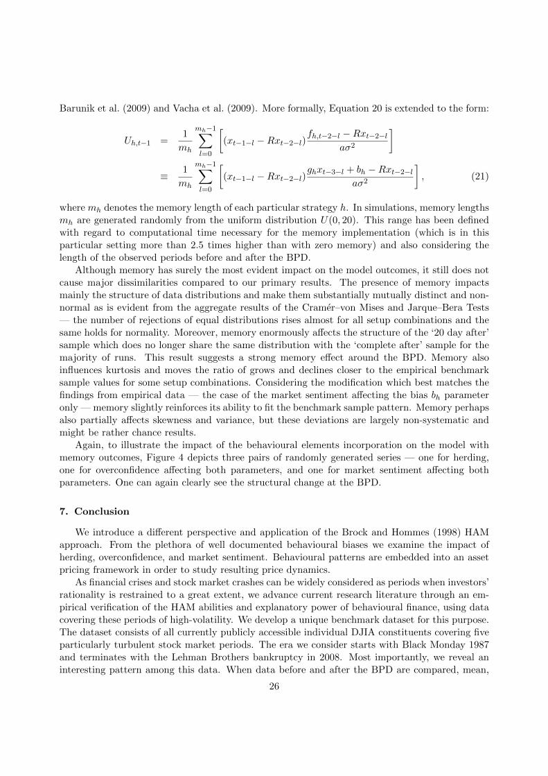
Barunik et al. (2009) and Vacha et al. (2009). More formally, Equation 20 is extended to the form:

Uh,t−1 =1

mh

mh−1∑l=0

[(xt−1−l −Rxt−2−l)

fh,t−2−l −Rxt−2−laσ2

]

≡ 1

mh

mh−1∑l=0

[(xt−1−l −Rxt−2−l)

ghxt−3−l + bh −Rxt−2−laσ2

], (21)

where mh denotes the memory length of each particular strategy h. In simulations, memory lengthsmh are generated randomly from the uniform distribution U(0, 20). This range has been definedwith regard to computational time necessary for the memory implementation (which is in thisparticular setting more than 2.5 times higher than with zero memory) and also considering thelength of the observed periods before and after the BPD.

Although memory has surely the most evident impact on the model outcomes, it still does notcause major dissimilarities compared to our primary results. The presence of memory impactsmainly the structure of data distributions and make them substantially mutually distinct and non-normal as is evident from the aggregate results of the Cramer–von Mises and Jarque–Bera Tests— the number of rejections of equal distributions rises almost for all setup combinations and thesame holds for normality. Moreover, memory enormously affects the structure of the ‘20 day after’sample which does no longer share the same distribution with the ‘complete after’ sample for themajority of runs. This result suggests a strong memory effect around the BPD. Memory alsoinfluences kurtosis and moves the ratio of grows and declines closer to the empirical benchmarksample values for some setup combinations. Considering the modification which best matches thefindings from empirical data — the case of the market sentiment affecting the bias bh parameteronly — memory slightly reinforces its ability to fit the benchmark sample pattern. Memory perhapsalso partially affects skewness and variance, but these deviations are largely non-systematic andmight be rather chance results.

Again, to illustrate the impact of the behavioural elements incorporation on the model withmemory outcomes, Figure 4 depicts three pairs of randomly generated series — one for herding,one for overconfidence affecting both parameters, and one for market sentiment affecting bothparameters. One can again clearly see the structural change at the BPD.

7. Conclusion

We introduce a different perspective and application of the Brock and Hommes (1998) HAMapproach. From the plethora of well documented behavioural biases we examine the impact ofherding, overconfidence, and market sentiment. Behavioural patterns are embedded into an assetpricing framework in order to study resulting price dynamics.

As financial crises and stock market crashes can be widely considered as periods when investors’rationality is restrained to a great extent, we advance current research literature through an em-pirical verification of the HAM abilities and explanatory power of behavioural finance, using datacovering these periods of high-volatility. We develop a unique benchmark dataset for this purpose.The dataset consists of all currently publicly accessible individual DJIA constituents covering fiveparticularly turbulent stock market periods. The era we consider starts with Black Monday 1987and terminates with the Lehman Brothers bankruptcy in 2008. Most importantly, we reveal aninteresting pattern among this data. When data before and after the BPD are compared, mean,

26

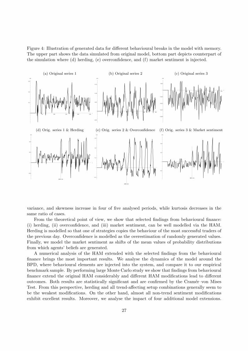
Figure 4: Illustration of generated data for different behavioural breaks in the model with memory.The upper part shows the data simulated from original model, bottom part depicts counterpart ofthe simulation where (d) herding, (e) overconfidence, and (f) market sentiment is injected.

(a) Original series 1

50 100 150 200 250t

0.1

0.2

0.3

xHtL

(b) Original series 2

50 100 150 200 250t

-0.05

0.05

0.10

0.15

xHtL

(c) Original series 3

50 100 150 200 250t

-0.20

-0.15

-0.10

-0.05

0.05

xHtL

(d) Orig. series 1 & Herding

BPD 126

t

-0.2

0.2

0.4

xHtL

(e) Orig. series 2 & Overconfidence

BPD 126

t

-0.1

0.1

0.2

0.3

xHtL

(f) Orig. series 3 & Market sentiment

BPD 126

t

-0.2

0.2

0.4

xHtL

variance, and skewness increase in four of five analysed periods, while kurtosis decreases in thesame ratio of cases.

From the theoretical point of view, we show that selected findings from behavioural finance:(i) herding, (ii) overconfidence, and (iii) market sentiment, can be well modelled via the HAM.Herding is modelled so that one of strategies copies the behaviour of the most successful traders ofthe previous day. Overconfidence is modelled as the overestimation of randomly generated values.Finally, we model the market sentiment as shifts of the mean values of probability distributionsfrom which agents’ beliefs are generated.

A numerical analysis of the HAM extended with the selected findings from the behaviouralfinance brings the most important results. We analyse the dynamics of the model around theBPD, where behavioural elements are injected into the system, and compare it to our empiricalbenchmark sample. By performing large Monte Carlo study we show that findings from behaviouralfinance extend the original HAM considerably and different HAM modifications lead to differentoutcomes. Both results are statistically significant and are confirmed by the Cramer–von MisesTest. From this perspective, herding and all trend-affecting setup combinations generally seem tobe the weakest modifications. On the other hand, almost all non-trend sentiment modificationsexhibit excellent results. Moreover, we analyse the impact of four additional model extensions.

27

These comprise the default presence of fundamentalists, stochastic formation of parameters, variousdifferent combinations, and memory. Generally, the first three modifications cause more or less onlyminor differences, while memory exhibits the most evident and statistically significant influence onthe model structure. Results further indicate that HAM is able to partially replicate price behaviourduring turbulent stock market periods. In particular, the market sentiment case affecting the biasparameter only exhibits a very good fit when compared to the empirical benchmark sample. Whenmemory is added into the system, a strong impact around the BPD is observed. Memory alsoreinforces the ability to fit the benchmark pattern for particular setup combinations.

To conclude, our approach suggests an alternative tool for examining the dynamics of changesin the HAM structure. To the best of our knowledge, this work also offers a first attempt tomatch the fields of HAM and behavioral finance in order to merge both approaches. We study theimpact of ‘behavioural breaks’ but other phenomena such as interest rate shocks or new suppliesof information might be implemented as well. As such, our work might be viewed as a step towardan intriguing extension of HAM — its empirical validation — while we show that it makes sense toconsider behavioural finance within the heterogeneous agent modelling framework and that bothapproaches can desirably complement one another.

References

Abdullah, W. A. T. W. (2003). Emergence of heterogeneity in an agent-based model. Physica A: Statistical Mechanicsand its Applications 324, 311–316.

Alfarano, S., T. Lux, and F. Wagner (2005). Estimation of agent-based models: The case of an asymmetric herdingmodels. Computational Economics 26, 19–49.

Baker, M. and J. Wurgler (2007). Investor sentiment in the stock market. The Journal of Economic Perspectives 21,129–151.

Baker, M. P., R. S. Ruback, and J. A. Wurgler (2005). Behavioral corporate finance: A survey. Technical report,NBER Working Papers.

Barber, B. M. and T. Odean (2000). Trading is hazardous to your wealth: The common stock investment performanceof individual investors. The Journal of Finance 55 (2), 773–806.

Barber, B. M. and T. Odean (2002). Online investors: Do the slow die first. Review of Financial Studies 15 (2),455–488.

Barberis, N., A. Shleifer, and R. Vishny (1998). A model of investor sentiment. Journal of Financial Economics 49,307–343.

Barberis, N. and R. H. Thaler (2003). Handbook of the Economics of Finance, Chapter 18: A Survey of BehavioralFinance, pp. 1051–1121. Elsevier Science B.V.

Barunik, J., L. Vacha, and M. Vosvrda (2009). Smart predictors in the heterogeneous agent model. Journal ofEconomic Interaction and Coordination 4, 163–172.

Bernardo, A. E. and I. Welch (2001). On the evolution of overconfidence and entrepreneurs. Journal of Economics& Management Strategy 10 (3), 301–330.

Biondi, Y., P. Giannoccolo, and S. Galam (2012). Formation of share market prices under heterogeneous beliefs andcommon knowledge. Physica A: Statistical Mechanics and its Applications 391 (22), 5532–5545.

Boswijk, H. P., C. H. Hommes, and S. Manzan (2007, February). Behavioral heterogeneity in stock prices. Journalof Economic Dynamics & Control 31 (2), 1938–1970.

Brock, W. A. and C. H. Hommes (1997). A rational route to randomness. Econometrica 65 (5), 1059–1095.Brock, W. A. and C. H. Hommes (1998). Heterogeneous beliefs and routes to chaos in a simple asset pricing model.

Journal of Economic Dynamics & Control 22, 1235–1274.Chang, S.-K. (2007). A simple asset pricing model with social interactions and heterogeneous beliefs. Journal of

Economic Dynamics & Control 31, 1300–1325.Chiarella, C., M. Gallegati, R. Leombruni, and A. Palestrini (2003). Asset price dynamics among heterogeneous

interacting agents. Computational Economics 22, 213–223.Chiarella, C. and X.-Z. He (2002a). An adaptive model on asset pricing and wealth dynamics with heterogeneous

trading strategies. Technical report, University of Technology, Sydney, Australia.

28

Chiarella, C. and X.-Z. He (2002b). Heterogeneous beliefs, risk and learning in a simple asset pricing model.Computational Economics 19, 95–132.

Daniel, K., D. Hirshleifer, and A. Subrahmanyam (1998). Investor psychology and security market under- andoverreactions. The Journal of Finance 53 (6), 1839–1855.

De Bondt, W. F. M. (1998). A portrait of the individual investor. European Economic Review 42, 831–844.De Bondt, W. F. M. and R. H. Thaler (1995). Handbooks in Operations Research and Management Science, Vol. 9,

Chapter 13: Financial Decision-Making in Markets and Firms: A Behavioral Perspective, pp. 385–410. Amster-dam: North Holland.

De Grauwe, P. and M. Grimaldi (2006). Exchange rate puzzles: A tale of switching attractors. European EconomicReview 50, 1–33.

de Jong, E., W. F. C. Verschoor, and R. C. J. Zwinkels (2009). Behavioural heterogeneity and shift-contagion:Evidence from the asian crisis. Journal of Economic Dynamics & Control 33, 1929–1944.

Diks, C., C. Hommes, and P. Zeppini (2013). More memory under evolutionary learning may lead to chaos. PhysicaA: Statistical Mechanics and its Applications 392 (4), 808–812.

Diks, C. and R. Weide (2005). Herding, a-synchronous updating and heterogeneity in memory in a cbs. Journal ofEconomic Dynamics & Control 29, 741–763.

Dong, L. (2007). Market behaviors and dynamic evolution on heterogeneous agent clusters. Physica A: StatisticalMechanics and its Applications 376 (0), 573–578.

Fama, E. F. (1970). Efficient capital markets: A review of theory and empirical work. The Journal of Finance 25 (2),383–417.

Ferreira, F. F., V. M. de Oliveira, A. F. Crepaldi, and P. R. Campos (2005). Agent-based model with heterogeneousfundamental prices. Physica A: Statistical Mechanics and its Applications 357, 534–542.

Frijns, B., T. Lehnert, and R. C. J. Zwinkels (2010). Behavioral heterogeneity in the option market. Journal ofEconomic Dynamics & Control 34, 2273–2287.

Goetzmann, W. N. and A. Kumar (2008). Equity portfolio diversification. Review of Finance 12, 433–463.Hirshleifer, D. (2001). Investor psychology and asset pricing. The Journal of Finance 56, 1533–1597.Hommes, C. H. (2006). Handbook of Computational Economics, Agent-Based Computational Economics, Chapter

Heterogeneous Agent Models in Economics and Finance, pp. 1109–1186. Elsevier Science B.V.Ising, E. (1925). Beitrag zur theorie des ferromagnetismus. Zeitschrift fur Physik 31 (1), 253–258.Kahneman, D. and A. N. Tversky (1974). Judgment under uncertainty: Heuristics and biases. Science 185, 1124–

1131.Kahneman, D. and A. N. Tversky (1979). Prospect theory: An analysis of decision under risk. Econometrica 47 (2),

263–291.Kaizoji, T., S. Bornholdt, and Y. Fujiwara (2002). Dynamics of price and trading volume in a spin model of stock

warkets with heterogeneous agents. Physica A: Statistical Mechanics and its Applications 316, 441–452.Kaltwasser, P. R. (2010). Uncertainty about fundamentals and herding behavior in the forex market. Physica A:

Statistical Mechanics and its Applications 389 (6), 1215–1222.Keynes, J. M. (1936). The General Theory of Employment, Interest, and Money. London: Macmillan.Kirman, A. (1991). Money and Financial Markets, Chapter Epidemics of Opinion and Speculative Bubbles in

Financial Markets, pp. 354–368. Macmillan, New York, USA.Kirman, A. (1993). Ants, rationality, and recruitment. The Quarterly Journal of Economics 108 (1), 137–156.Lamba, H. and T. Seaman (2008). Rational expectations, psychology and inductive learning via moving thresholds.

Physica A: Statistical Mechanics and its Applications 387 (15), 3904–3909.LeBaron, B. (2005). Agent-based computational finance. Technical report, International Business School, Brandeis

University, USA.Liu, X., S. Gregor, and J. Yang (2008). The effects of behavioral and structural assumptions in artificial stock

market. Physica A: Statistical Mechanics and its Applications 387 (11), 2535–2546.Lucas, R. E. J. (1972). Expectations and the neutrality of money. Journal of Economic Theory 4 (2), 103–124.Lucas, R. E. J. (1978). Asset prices in an exchange economy. Econometrica 46, 1429–1445.Malkiel, B. G. (2003). The efficiency market hypothesis and its critics. Journal of Economic Perspectives 17, 59–82.Muth, J. F. (1961). Rational expectations and the theory of price movements. Econometrica 29 (3), 315–335.Odean, T. (1998). Are investors reluctant to realize their losses? Journal of Finance 53, 1775–1798.Odean, T. (1999). Do investors trade too much? American Economic Review 89, 1279–1298.Onsager, L. (1944, Feb). Crystal statistics. i. a two-dimensional model with an order-disorder transition. Phys.

Rev. 65, 117–149.Sansone, A. and G. Garofalo (2007). Asset price dynamics in a financial market with heterogeneous trading strategies

29

and time delays. Physica A: Statistical Mechanics and its Applications 382 (1), 247–257.Sargent, T. J. (1993). Bounded Rationality in Macroeconomics. Oxford: Clarendon Press.Scheinkman, J. and W. Xiong (2004). Heterogeneous beliefs, speculation and trading in financial markets. Technical

report, Princeton University, USA.Schleifer, A. and L. H. Summers (1990). The noise trader approach to finance. The Journal of Economic Perspec-

tives 4 (2), 19–33.Schutz, G. M., F. P. de Almeida Prado, R. J. Harris, and V. Belitsky (2009). Short-time behaviour of demand and

price viewed through an exactly solvable model for heterogeneous interacting market agents. Physica A: StatisticalMechanics and its Applications 388 (19), 4126–4144.

Shiller, R. J. (2000). Measuring bubble expectations and investor confidence. The Jornal of Psychology and FinancialMarkets 1 (1), 49–60.

Shiller, R. J. (2003). From efficient markets theory to behavioral finance. Journal of Economic Perspectives 17 (1),83–104.

Shimokawa, T., K. Suzuki, and T. Misawa (2007). An agent-based approach to financial stylized facts. Physica A:Statistical Mechanics and its Applications 379 (1), 207–225.

Simon, H. A. (1955). A behavioral model of rational choice. The Quarterly Journal of Economics 69 (1), 99–118.Simon, H. A. (1957). Models of Man. New York: Wiley.Svenson, O. (1981). Are we all less risky and more skillful than our fellow drivers? Acta Psychologica 47, 143–148.Vacha, L., J. Barunik, and M. Vosvrda (2009). Smart agents and sentiment in the heterogeneous agent model. Prague

Economic Papers 3, 209–219.Vacha, L., J. Barunik, and M. Vosvrda (2012). How do skilled traders change the structure of the market. Interna-

tional Review of Financial Analysis 23, 66–71.Westerhoff, F. H. (2004). Greed, fear and stock market dynamics. Physica A: Statistical Mechanics and its Applica-

tions 343 (0), 635–642.Zhu, M., C. Chiarella, X.-Z. He, and D. Wang (2009). Does the market maker stabilize the market? Physica A:

Statistical Mechanics and its Applications 388, 3164–3180.

Appendix

30

Tab

le6:

DJIA

Com

pon

ents

1987

–200

8

Eve

nt

Per

iod

Sto

cks

(tic

ker

sym

bol

s)#

Bla

ckM

on

day

Sep

t21

–O

ct19,

198

7A

A,

AX

P,

BA

,C

VX

,D

D,

EK

,F

L,

GE

,G

M,

GT

,H

ON

,IB

M,

IP,

KO

,M

CD

,M

MM

,M

O,

MR

K,

NA

V,

PG

,T

,U

TX

,X

OM

;N

/A:

BS

,P

RI,

‘old

’S

,T

X,

UK

,‘o

ld’

WX

,X

n

460

Oct

19

–N

ov16,

198

7–||–

460

Ru

ble

Dev

alu

ati

on

Ju

l20

–A

ug

17,

1998

AA

,A

XP

,B

A,

C,

CA

T,

CV

X,

DD

,D

IS,

EK

,G

E,

GM

,G

T,

HO

N,

HP

Q,

IBM

,IP

,JN

J,

JP

M,

KO

,M

CD

,M

MM

,M

O,

MR

K,

PG

,T

,U

TX

,W

MT

,X

OM

;N

/A:

‘old

’S

,U

K

560

Au

g17

–S

ep15,

1998

–||–

560

Dot

-com

Bu

bb

leF

eb10

–M

ar10

,2000

AA

,A

XP

,B

A,

C,

CA

T,

DD

,D

IS,

EK

,G

E,

GM

,H

D,

HO

N,

HP

Q,

IBM

,IN

TC

,IP

,JN

J,

JP

M,

KO

,M

CD

,M

MM

,M

O,

MR

K,

MSF

T,

PG

,T

,U

TX

,W

MT

,X

OM

;N

/A:

IPon

lyfo

rF

eb23

,20

00,

SB

C

579

Mar

10

–A

pr

7,

2000

–||–

580

WT

C9/1

1A

ttack

Au

g10

–S

ep10

,200

1A

A,

AX

P,

BA

,C

,C

AT

,D

D,

DIS

,E

K,

GE

,G

M,

HD

,H

ON

,H

PQ

,IB

M,

INT

C,

IP,

JN

J,

JP

M,

KO

,M

CD

,M

MM

,M

O,

MR

K,

MSF

T,

PG

,T

,U

TX

,W

MT

,X

OM

;N

/A:

SB

C

580

Sep

10

–O

ct12,

2001

–||–

580

Leh

man

Bro

ther

sA

ug

15

–S

ep15,

2008

AA

,A

XP

,B

A,B

AC

,C

,C

AT

,C

VX

,D

D,D

IS,G

E,G

M,H

D,H

PQ

,IB

M,IN

TC

,JN

J,

JP

M,

KO

,M

CD

,M

MM

,M

RK

,M

SF

T,

PF

E,

PG

,T

,U

TX

,V

Z,

WM

T,

XO

M;

omit

ted

asan

outl

ier:

AIG

580

Sep

15

–O

ct13,

2008

–||–

,bu

tom

itte

dA

IGw

asre

pla

ced

by

KF

Ton

Sep

tem

ber

22,

2008

—w

eom

itK

FT

asw

ell

toke

epd

atas

etco

nsi

sten

cy58

0

Note:#

standsfornumber

ofobservations.

N/A

standsforstock

notavailable

foraparticularperiod.

‘old’den

otesco

mpanieswhichhistorica

lticker

symbolis

nowadaysusedforanoth

erco

mpany.

31

Behavioural breaks in the heterogeneous agent model: the impact of herding, overconfidence, and market sentiment

Documents