1 BEHAVIOUR AND DESIGN OF STEEL FIBRE REINFORCED CONCRETE SLABS A thesis submitted to Imperial College London in partial fulfilment of the requirements for the degree of Doctor of Philosophy in the Faculty of Engineering by SOTIRIOS OIKONOMOU-MPEGETIS B.Eng. (Hons), M.Sc., D.I.C. Structural Engineering Research Group Department of Civil and Environmental Engineering Imperial College London London, SW7 2AZ

Welcome message from author
This document is posted to help you gain knowledge. Please leave a comment to let me know what you think about it! Share it to your friends and learn new things together.
Transcript
1
BEHAVIOUR AND DESIGN OF STEEL FIBRE
REINFORCED CONCRETE SLABS
A thesis submitted to Imperial College London in partial fulfilment of the requirements for the
degree of Doctor of Philosophy in the Faculty of Engineering
by
SOTIRIOS OIKONOMOU-MPEGETIS
B.Eng. (Hons), M.Sc., D.I.C.
Structural Engineering Research Group
Department of Civil and Environmental Engineering
Imperial College London
London, SW7 2AZ

2
In loving memory of my father who passed away on the 22nd of August 2012

3
Declaration
The work presented in this dissertation was carried out in the Department of Civil and
Environmental Engineering at Imperial College London from October 2009. This thesis is the result of
my own work and any quotation from, or description of the work of others is acknowledged herein
by reference to the sources, whether published or unpublished.
This dissertation is not the same as any that I have submitted for any degree, diploma or other
qualification at any other university. No part of this thesis has been or is being concurrently
submitted for any such degree or other qualification.
The copyright of this thesis rests with the author and is made available under a Creative Commons
Attribution Non-Commercial No Derivatives licence. Researchers are free to copy, distribute or
transmit the thesis on the condition that they attribute it, that they do not use it for commercial
purposes and that they do not alter, transform or build upon it. For any reuse or redistribution,
researchers must make clear to others the licence terms of this work.
Sotirios Oikonomou-Mpegetis
London, September 2013
4
Abstract
Using Steel Fibre Reinforced Concrete (SFRC) can bring substantial benefits to the construction
industry of which savings in construction time and labour are most significant. In addition, steel
fibres enhance crack control particularly when acting in conjunction with reinforcement bars.
Despite the aforementioned benefits of SFRC, there is a still a lack of consensus on the principles
that should be adopted in its design. Currently, a number of different test methods are used to
determine the material properties of SFRC but there is no agreement on which method is best. As a
result, steel fibre suppliers claim widely differing properties for similar fibres which leads to
confusion amongst designers and in some cases inadequate structural performance.
This research considers the design of SFRC slabs with emphasis on pile supported slabs which are
frequently designed using proprietary methods due to the absence of codified guidance. Key issues
in the design of such slabs are control of cracking in service and the calculation of flexural and
punching shear resistances. A fundamental challenge is that SFRC exhibits a strain softening
response at the dosages commonly used in slabs. At present, the yield line method is generally
considered most suitable for designing such slabs at the ultimate limit state but there is a lack of
consensus on the design moment of resistance as the bending moment along the yield lines reduces
with increasing crack width. This thesis investigates these matters using a combination of
experimental and theoretical work. The experimental work compares material properties derived
from notched beam and round plate tests and seeks to determine a relationship between the two.
Tests were also carried out on continuous slabs with the same material properties as used in the
notched beam and round plate tests. Round plate tests were also carried out to determine the
contribution of steel fibres to punching shear resistance. The theoretical work investigates the
applicability of yield line analysis to the design of SFRC slabs using a combination of numerical
modelling and design oriented analytical models. Design for punching shear and the serviceability
limit state of cracking are also considered.

5
Acknowledgements
I would like to express my heartfelt gratitude to my supervisor Dr. Robert Vollum. His advice and
guidance has been instrumental in the completion of this thesis. I would like to thank him for all the
time that he has invested in me and all the knowledge that he transferred to me all these years. His
support and kindness will always be remembered.
I would like to express my gratitude to Dr. Ali Abbas for his advice and for giving me the opportunity
to undertake a PhD in Imperial College London. A special mention should be made to the technicians
at the Structures Lab at Imperial College for their good work in the experimental part of this project.
I would like to thank my family for their support during my education. Their encouragement guided
me through all the good and the bad times. Special recognition is due to my wonderful mother for
her endless encouragement and kindness.
I want to dedicate this thesis to the loving memory of my father whose endless sacrifices made this
work possible.

6
Table of Contents
Declaration .............................................................................................................................................. 3
Abstract ................................................................................................................................................... 4
Acknowledgements ................................................................................................................................. 5
Table of Contents .................................................................................................................................... 6
List of Figures ........................................................................................................................................ 14
List of Tables ......................................................................................................................................... 26
List of Symbols ...................................................................................................................................... 27
Introduction .......................................................................................................................................... 29
1.1 Background ........................................................................................................................... 29
1.2 Objectives.............................................................................................................................. 32
1.3 Research Methodology ......................................................................................................... 32
1.4 Outline of Thesis ................................................................................................................... 33
Literature Review .................................................................................................................................. 35
2.1 Introduction .......................................................................................................................... 35
2.2 Historical Development of Steel Fibre Reinforced Concrete ................................................ 35
2.2.1 Origin of Steel-Fibre Reinforced Concrete .................................................................... 35
2.2.2 Historical Development ................................................................................................ 36
2.3 Intrinsic Properties of Steel Fibre Reinforced Concrete ....................................................... 37
2.3.1 Relevant Mechanics Concepts of Fibre-Reinforced Composites .................................. 37
2.3.2 Tensile Behaviour of Steel Fibre Reinforced Concrete ................................................. 37
2.3.3 Compressive Behaviour of Steel Fibre Reinforced Concrete ........................................ 39
2.3.4 Flexural Behaviour and Fracture Toughness of Steel Fibre Reinforced Concrete ........ 40
2.4 Current Testing Practice for Steel Fibre Reinforced Concrete .............................................. 42
2.4.1 Background ................................................................................................................... 42
2.4.2 Beam (Bending) Tests ................................................................................................... 42
2.4.3 Slab and Plate Tests ...................................................................................................... 47
7
2.4.4 Critical Assessment of Testing Methods ....................................................................... 49
2.5 Constitutive Behaviour of Steel Fibre Reinforced Concrete ................................................. 52
2.5.1 Introduction to SFRC Constitutive Modelling and Research Background ..................... 52
2.5.2 Stress-Crack Width Philosophy ..................................................................................... 52
2.5.3 Stress-Strain Approach .................................................................................................. 62
2.5.4 Crack Band Width .......................................................................................................... 65
2.5.5 Critical Review of Constitutive Modelling Concepts ..................................................... 66
2.6 Concluding Remarks .............................................................................................................. 67
Design of SFRC Pile Supported Slabs ..................................................................................................... 68
3.1 Background ........................................................................................................................... 68
3.2 Design Aspects ...................................................................................................................... 68
3.2.1 General Overview ......................................................................................................... 68
3.2.2 Anatomy of a Pile Supported Slab ................................................................................ 68
3.2.3 Design Loading .............................................................................................................. 69
3.2.4 Pathology of Pile – Supported Slabs ............................................................................. 69
3.3 Elastic Design ........................................................................................................................ 70
3.4 Yield Line Method ................................................................................................................. 71
3.5 Punching Shear ..................................................................................................................... 76
3.6 Serviceability Limit States ..................................................................................................... 79
3.6.1 Restrained Shrinkage .................................................................................................... 79
3.6.2 Cracking ......................................................................................................................... 80
3.6.3 Deflection ...................................................................................................................... 81
3.7 Shortcomings of Current Design Guidelines ......................................................................... 81
3.8 Concluding Remarks .............................................................................................................. 83
Experimental Programme ..................................................................................................................... 85
4.1 Introduction .......................................................................................................................... 85
4.2 Summary of Tests .................................................................................................................. 85
4.3 Fabrication of Test Specimens .............................................................................................. 87
8
4.3.1 Concrete Mix Design ..................................................................................................... 87
4.3.2 Casting and curing of specimens ................................................................................... 88
4.4 Beam Tests ............................................................................................................................ 89
4.4.1 Geometry of Test Specimens ........................................................................................ 89
4.4.2 Instrumentation ............................................................................................................ 90
4.4.3 Testing Procedure ......................................................................................................... 92
4.5 Statically Determinate Plate Tests ........................................................................................ 92
4.5.1 Geometry of Test Specimens ........................................................................................ 92
4.5.2 Instrumentation ............................................................................................................ 93
4.5.3 Testing Procedure ......................................................................................................... 95
4.6 Statically Indeterminate Plate Tests ..................................................................................... 96
4.6.1 Geometry of Test Specimens ........................................................................................ 96
4.6.2 Instrumentation and Testing ........................................................................................ 99
4.6 Crack widths in Round Determinate Panel Tests .................................................................. 99
4.6.1 Test setup ...................................................................................................................... 99
4.6.2 Instrumentation .......................................................................................................... 100
4.6.3 Testing Procedure ....................................................................................................... 103
4.7 Damaged Determinate Round Panel Tests under Reloading ............................................. 104
4.7.1 Test setup .................................................................................................................... 104
4.7.2 Testing Procedure ....................................................................................................... 104
4.8 Statically Indeterminate Slab Tests ..................................................................................... 105
4.8.1 Geometry of Test Specimens ...................................................................................... 105
4.8.2 Test Setup ................................................................................................................... 106
4.8.3 Instrumentation .......................................................................................................... 107
4.8.4 Testing Procedure ....................................................................................................... 110
4.9 Statically Indeterminate Slab Tests with Restraint ............................................................. 110
4.9.1 General considerations ............................................................................................... 110
4.9.2 Test Setup ................................................................................................................... 111

9
4.9.3 Instrumentation and Testing Procedure ..................................................................... 113
4.10 Punching Shear Tests .......................................................................................................... 113
4.10.1 General considerations ............................................................................................... 113
4.11 Concluding Remarks ............................................................................................................ 116
Experimental Results .......................................................................................................................... 117
5.1 General Remarks ................................................................................................................. 117
5.2 Control Specimens .............................................................................................................. 117
5.2.1 General Overview ....................................................................................................... 117
5.2.2 Compressive Test ........................................................................................................ 117
5.2.3 Splitting ‘Brazilian’ Test ............................................................................................... 118
5.3 Notched Beam Tests ........................................................................................................... 118
5.3.1 Failure Mechanism ...................................................................................................... 118
5.3.3 Load – Deflection Response ........................................................................................ 119
5.3.4 Fibre Distribution and Orientation .............................................................................. 123
5.3.5 Residual strength – CMOD Response ......................................................................... 128
5.3.6 Displacement – CMOD Response ................................................................................ 133
5.4 Statically Determinate Round Plate Tests ........................................................................... 136
5.4.1 General Overview ....................................................................................................... 136
5.4.2 Results ......................................................................................................................... 136
5.5 Statically Indeterminate Round Plate Tests ........................................................................ 141
5.5.1 General Overview ....................................................................................................... 141
5.5.2 Structural Response .................................................................................................... 141
5.6 Additional Statically Determinate Round Panel Tests ........................................................ 147
5.6.1 General Remarks ......................................................................................................... 147
5.6.2 Load – Deflection Behaviour ....................................................................................... 147
5.6.3 Crack Widths ............................................................................................................... 150
5.6.4 Crack Width along a Fracture Surface ......................................................................... 160
5.6.5 Crack Profile through the thickness ............................................................................ 163
10
5.7 Damaged Determinate Round Panel Tests under Reloading ............................................. 166
5.7.1 General Remarks ......................................................................................................... 166
5.7.2 Load – Deflection Behaviour ....................................................................................... 166
5.7.3 Crack Width Development .......................................................................................... 169
5.7.4 Crack Width along a Fracture Surface ......................................................................... 173
5.8 Slab Tests ............................................................................................................................ 178
5.8.1 Failure Mechanism ...................................................................................................... 178
5.8.2 Crack Width ................................................................................................................. 181
5.9 Slab Tests with Axial Restraint ............................................................................................ 186
5.9.1 Test Results ................................................................................................................. 186
5.10 Punching Shear Tests .......................................................................................................... 191
5.10.1 Test Results ................................................................................................................. 191
5.11 Concluding Remarks ............................................................................................................ 196
Numerical Methodology ..................................................................................................................... 197
6.1 General Remarks ................................................................................................................. 197
6.2 Review of the Finite Element Method ................................................................................ 197
6.2.1 Linear Finite Element Analysis .................................................................................... 197
6.2.2 Non-Linear Finite Element Analysis ............................................................................ 199
6.3 Constitutive Modelling Approaches in NLFEA .................................................................... 200
6.3.1 General Overview ....................................................................................................... 200
6.3.2 Discrete cracking ......................................................................................................... 200
6.3.3 Smeared cracking ........................................................................................................ 201
6.3.4 Solution procedure adopted ....................................................................................... 201
6.4 Constitutive Modelling Approaches Adopted ..................................................................... 203
6.4.1 Introduction to Concrete Constitutive Modelling Approaches................................... 203
6.4.2 Concrete Smeared Cracking (Inelastic Constitutive Model) ....................................... 203
6.4.3 Concrete Damaged Plasticity ...................................................................................... 206
6.4.4 Brittle Concrete Cracking ............................................................................................ 207
11
6.4.5 Choice of Material Model ........................................................................................... 209
6.5 Constitutive Model Adopted ............................................................................................... 210
6.5.1 Introductory Principles ................................................................................................ 210
6.5.2 Uni-axial tension and compression conditions ........................................................... 211
6.5.3 Post-Failure Tensile behaviour .................................................................................... 212
6.5.4 Post-Failure Compressive behaviour .......................................................................... 213
6.5.5 Plastic Flow .................................................................................................................. 214
6.5.6 Yield Function .............................................................................................................. 214
6.6 Material Parameters used in Damaged Plasticity Model.................................................... 216
6.6.1 General Remarks ......................................................................................................... 216
6.6.2 Poisson’s ratio ............................................................................................................. 216
6.6.3 Elastic (Young’s) Modulus ........................................................................................... 217
6.6.4 Uniaxial Compressive Behaviour ................................................................................. 217
6.6.5 Uniaxial Tensile Behaviour .......................................................................................... 217
6.6.6 Plastic Flow .................................................................................................................. 217
6.6.7 Ratio of Biaxial to Uniaxial Compressive Strength ...................................................... 218
6.7 Concluding Remarks ............................................................................................................ 218
Numerical Modelling of Structural Tests ............................................................................................ 219
7.1 General Remarks ................................................................................................................. 219
7.2 Inverse Analysis of Notched Beam Tests using Discrete Cracking ...................................... 219
7.2.1 General Overview ....................................................................................................... 219
7.2.2 Inverse analysis modelling .......................................................................................... 221
7.2.3 Input Parameters ........................................................................................................ 222
7.2.4 Non Linear Finite Element Analysis (NLFEA) ............................................................... 223
7.3 Analysis of Round Determinate Plate ................................................................................. 228
7.3.1 Introduction to Yield Line Analysis .............................................................................. 228
7.3.2 Yield Line Analysis of Statically Determinate Round Panel ......................................... 228
7.4 Comparative Analysis of RDP with NLFEA and Yield Line Analysis ..................................... 230
12
7.4.1 Input Parameters ........................................................................................................ 230
7.4.2 Results of analysis of RDP tests ................................................................................... 231
7.4.3 Moment along the Yield Line ...................................................................................... 234
7.4.4 Rotation along yield lines ............................................................................................ 244
7.4.5 Crack width along the yield line .................................................................................. 247
7.4.6 Derivation of EN 14651 residual concrete strengths from RDP tests ......................... 251
7.4.7 Comparison of variability of residual strengths determined from RDP and notched
beams 256
7.5 Smeared Cracking Inverse Analysis of the RDP ................................................................... 261
7.5.1 General Overview ....................................................................................................... 261
7.5.2 Smeared crack inverse analysis of the RDP ................................................................ 262
7.6 Wide Beam Failure Mechanism - Two Span Slab Tests ...................................................... 264
7.6.1 General Overview ....................................................................................................... 264
7.6.2 Yield Line Analysis of Wide Beam Failure Mechanism ................................................ 264
7.6.4 Smeared Cracking Approach ....................................................................................... 266
7.6.5 Discrete Cracking Approach ........................................................................................ 269
7.6.6 Comparison of predicted and measured crack widths ............................................... 274
7.6.7 Comparison of the discrete and smeared cracking approaches for the two span slabs
277
7.6.8 Effect of additional restraint on the structural behaviour .......................................... 279
7.7 Punching Shear Tests .......................................................................................................... 282
7.7.1 General Remarks ......................................................................................................... 282
7.6.2 Material Properties and Flexural Resistance .............................................................. 283
7.7.3 Analysis of Punching Shear Tests ................................................................................ 285
7.7.4 Comparison with EC2 and design recommendations in TR34 4th Edition ................... 287
7.8 Concluding Remarks ............................................................................................................ 288
Analysis of Pile Supported Slabs ......................................................................................................... 290
8.1 General Remarks ................................................................................................................. 290
13
8.2 Discrete Cracking Approach ................................................................................................ 290
8.2.1 General modelling considerations .............................................................................. 290
8.2.2 Non Linear Finite Element Analysis (NLFEA) ............................................................... 292
8.2.3 Moment distribution along the Yield Line .................................................................. 298
8.2.4 Rotation along the Yield Line ...................................................................................... 302
8.2.5 Effect of axial restraint ................................................................................................ 307
8.3 Smeared Cracking Approach ............................................................................................... 310
8.3.1 General modelling considerations .............................................................................. 310
8.3.2 Structural Response of Pile Supported Slab under UDL – Smeared crack analysis .... 313
8.4 Concluding Remarks and Recommended Considerations .................................................. 316
8.4.1 Recommended considerations for SFRC slabs ............................................................ 317
Conclusions ......................................................................................................................................... 319
9.1 Recapitulation ..................................................................................................................... 319
9.2 Conclusions from literature survey ..................................................................................... 320
9.3 Shortcomings of current design guidelines ........................................................................ 320
9.4 Conclusions from experimental work ................................................................................. 321
9.5 Conclusions from present NLFEA ........................................................................................ 322
9.5 Recommended Considerations ........................................................................................... 323
9.6 Recommendations for future research ............................................................................... 324
Bibliography ........................................................................................................................................ 325
APPENDIX ............................................................................................................................................ 341
APPENDIX A: ........................................................................................................................................ 342
APPENDIX B: ........................................................................................................................................ 346
APPENDIX C: ........................................................................................................................................ 351
14
List of Figures
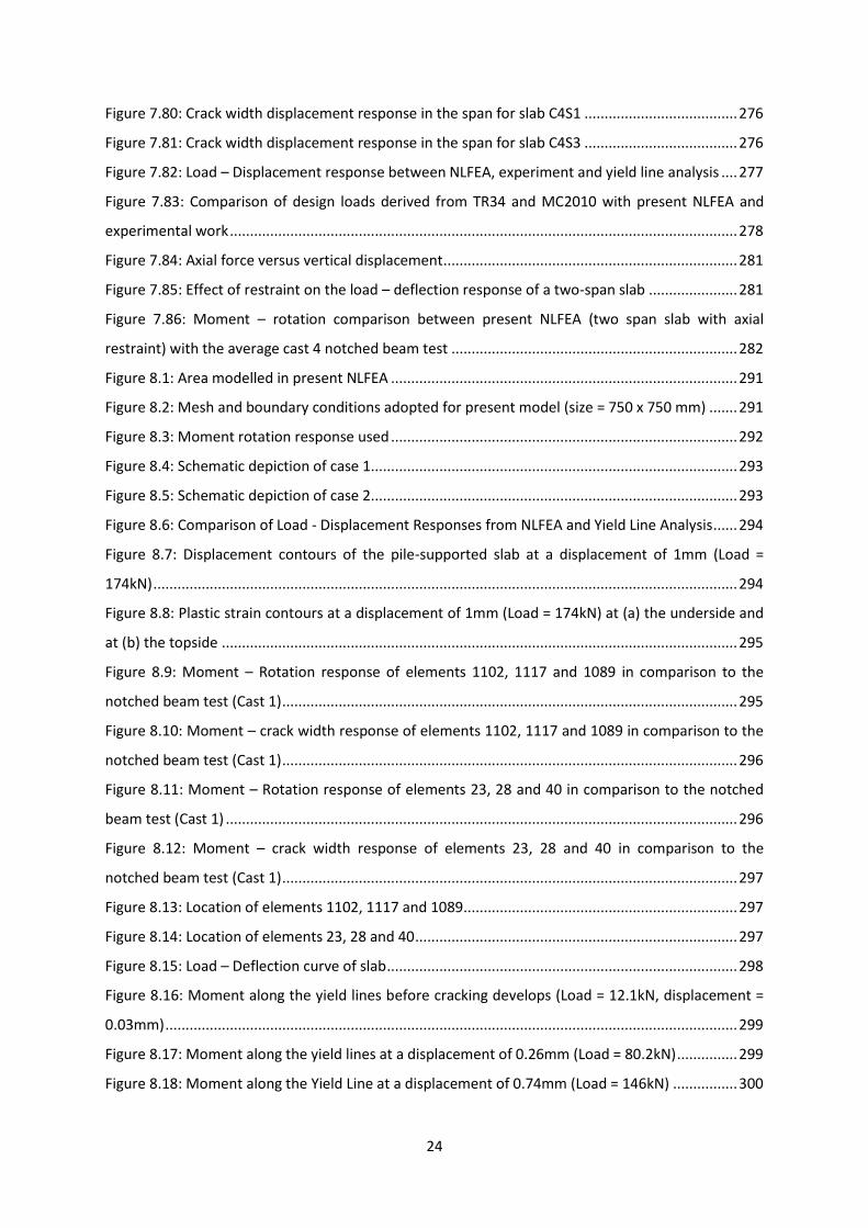
Figure 1.1: Layout of a typical pile-supported slab, (adopted from
http://www.twintec.co.uk/products_freetop.asp) .............................................................................. 29
Figure 1.2: Cross-section of typical pile-supported slabs, as adopted from (The Concrete Society,
2003) ..................................................................................................................................................... 30
Figure 1.3: Typical steel fibres used in industrial applications, such as the construction of pile-
supported slabs (adopted from http://www.mswukltd.co.uk/dramix_steelfibres.htm) ..................... 32
Figure 2.1: Schematic depiction of tensile response for different dosages of steel fibres (from Maild,
2005 as cited in Kooiman, 2000) ........................................................................................................... 38
Figure 2.2: Depiction of typical SFRC and plain concrete specimen when subjected to compression
(Konig & Kutzing, as cited in Kooiman, 2000) ....................................................................................... 40
Figure 2.3: Typical Response of SFRC in Flexure (Barros & Figueiras, 1999) ........................................ 41
Figure 2.4: Typical stress distributions in a concrete section subjected to four-point bending (Tlemat,
Pilakoutas, & Neocleous, 2006) ............................................................................................................ 41
Figure 2.5: Three-point and Four-point bending configurations, as adopted from (Kooiman, 2000) .. 42
Figure 2.6: Definition of fracture toughness values Df,2 and Df,3 , adapted from (RILEM, 2000) as cited
in (Kooiman, 2000) ................................................................................................................................ 44
Figure 2.7: Correspondence of flexural load and CMOD, adopted from (British Standards Institution,
2005) ..................................................................................................................................................... 45
Figure 2.8: Schematic Illustration of the ASTM C 1550 statically determinate round panel test, as
adopted from (Bernard, 2005) .............................................................................................................. 48
Figure 2.9: Anatomy of a crack propagating through plain concrete, as suggested by the Fictitious
Crack Model framework (Karihaloo, 1995) ........................................................................................... 53
Figure 2.10: Anatomy of a crack propagating through SFRC, as suggested by the Fictitious Crack
Model framework (RILEM, 2002) .......................................................................................................... 54
Figure 2.11: Distribution of the bond stresses along a set of fibres at a crack width w, adopted from
(Hillerborg, 1980) .................................................................................................................................. 54
Figure 2.12: Schematic representation of the cracked hinge concept as formulated by Pedersen,
adapted from (RILEM, 2002) ................................................................................................................. 56
Figure 2.13: Schematic representation of the cracked hinge using independent spring elements as
proposed by Olesen, from (Olesen, 2001) ............................................................................................ 59
Figure 2.14: Tri-linear tension softening relation, as adopted from (Barros et al., 2005) .................... 60
15
Figure 2.15: Schematic Illustration of the (a) rigid plastic and (b) linear models applied in Model Code
2010 (International Federation for Structural Concrete, 2010) ........................................................... 61
Figure 2.16: Stress-strain relationship, as adapted from (RILEM, 2003) .............................................. 63
Figure 2.17: Definition of the size factor h , as adapted from (RILEM, 2003) ..................................... 64
Figure 2.18: Crack band width approach developed by Bazant and Oh (1983), diagram adopted from
(Kooiman, 2008) .................................................................................................................................... 66
Figure 3.1: Schematic depiction of the wide beam failure mechanism in a pile-supported ground
floor, as adopted from (Kennedy and Goodchild, 2003) ...................................................................... 72
Figure 3.2: Folded Plate Failure Mechanism in (a) an exterior (perimeter) and (b) in an interior panel
under uniformly distributed load, adopted from (The Concrete Society, 2012) .................................. 72
Figure 3.3: Folded Plate Failure Mechanism in (a) an exterior (perimeter) and (b) in an interior panel
under concentrated line load, adopted from (The Concrete Society, 2012) ........................................ 73
Figure 3.4: Schematic depiction of the circular fan failure mechanism in a pile-supported ground
floor, as adapted from (Kennedy and Goodchild, 2003) ...................................................................... 74
Figure 3.5: Definition of the critical perimeter for punching shear at the pile head and at the point
load, adopted from (The Concrete Society, 2012) ................................................................................ 79
Figure 4.1: Casting mould for the standard beam specimens .............................................................. 88
Figure 4.2: Casting mould for the round panel specimens ................................................................... 89
Figure 4.3: Casting mould for the long beam tests ............................................................................... 89
Figure 4.4: Three-point bending beam test adopted for the present study, as per the
recommendations of BS EN 14651 ....................................................................................................... 90
Figure 4.5: Recommended arrangement for measuring the CMOD (adopted from BS EN 14651:2005)
.............................................................................................................................................................. 91
Figure 4.6: Test setup for the three-point bending beam test ............................................................. 91
Figure 4.7: Displacement transducer detail .......................................................................................... 91
Figure 4.8: Statically determinate round panel test adopted for the current research study ............. 93
Figure 4.9: Set-up of the specimen onto the test rig ............................................................................ 94
Figure 4.10: Underside of the specimen just before the commencement of the testing .................... 94
Figure 4.11: Support structure details for the statically determinate round panel test (a) showing the
transfer plates and (b) showing the supports ....................................................................................... 95
Figure 4.12: Statically indeterminate round panel test adopted for the current research study ........ 96
Figure 4.13: Positioning of the (a) statically indeterminate test specimen onto the supports and (b)
detail of the support structure used ..................................................................................................... 97

16
Figure 4.14: LVDT used to (a) measure the vertical displacement (b) the bedding – in of the steel
support (c) the deflection of the support structure relative to the laboratory floor ........................... 98
Figure 4.15: Test setup used for the measuring of the crack widths.................................................. 100
Figure 4.16: Load plate placed on the underside of the specimen .................................................... 100
Figure 4.17: Demec points on the topside (tension side) of the specimen in question ..................... 101
Figure 4.18: Positioning of Demec points and Demec point reading references ............................... 101
Figure 4.19: Positioning of Linear Variable Displacement Transducers under each support ............. 102
Figure 4.20: Actuator used for the present experiment ..................................................................... 103
Figure 4.21: Test setup of for the two-span slab (a) side view (b) section through the slab ............. 105
Figure 4.22: Details of the supports used in the present experiment (a) side view (b) front view .... 106
Figure 4.23: Instron actuator and spreader beam used in the present experimental setup ............. 106
Figure 4.24: Load bearing detail ......................................................................................................... 107
Figure 4.25: Demec points used to record the total strain and the crack width ................................ 107
Figure 4.26: Arrangement of Demec points on to the slab (a) top view (b) side 1 (c) side 2 ............. 108
Figure 4.27: LVDT used to measure the span displacement ............................................................... 108
Figure 4.28: LVDT used to measure the bedding in of the slab onto (a) the middle support and (b) the
supports .............................................................................................................................................. 109
Figure 4.29: Load cells used for the measuring of load at each of the three supports ...................... 109
Figure 4.30: Displacement transducer mounted along the crack ....................................................... 110
Figure 4.31: Experimental setup, using a restraint frame .................................................................. 111
Figure 4.32: Details of restraining frame (a) and (b) show the pumps installed either side of the frame
and (c) shows the connecting steel..................................................................................................... 112
Figure 4.33: Depiction of statically determinate round plate test ..................................................... 114
Figure 4.34: Depiction of punching test type 1, with a single B16 hoop ............................................ 115
Figure 4.35: Depiction of punching test type 2, with two B16 hoops ................................................ 115
Figure 4.36: Loading arrangement of punching shear tests ............................................................... 116
Figure 5.1: Failure mode of three point bending beam with a single crack ....................................... 119
Figure 5.2: Three point bending beam load – deflection response for Cast 1 ................................... 121
Figure 5.3: Three point bending beam load – deflection response for Cast 2 ................................... 121
Figure 5.4: Three point bending beam load – deflection response for Cast 3 ................................... 122
Figure 5.5: Three point bending beam load – deflection response for Cast 4 ................................... 122
Figure 5.6: Characteristic mode of failure of a three-point bending beam test under flexure .......... 123
Figure 5.7: Balling of fibres in test specimen C2B6 ............................................................................. 123
Figure 5.8: Division of the beam cross-sectional area to evaluate the fibre distribution .................. 124
17
Figure 5.9: Number of fibres through the cross section for Beams in C1 ........................................... 124
Figure 5.10: Amount of fibres through the cross section for Beams in C2 ......................................... 125
Figure 5.11: Amount of fibres through the cross section for Beams in C3 ......................................... 126
Figure 5.12: Cross-section of beams (a) C3B1 and (b) C3B4 ............................................................... 127
Figure 5.13: Amount of fibres through the cross section for Beams in C4 ......................................... 127
Figure 5.14: Displacement transducer for the measurement of the CMOD ...................................... 128
Figure 5.15: Residual flexural tensile strength vs CMOD for the three point bending beams in cast C1
............................................................................................................................................................ 129
Figure 5.16: Residual flexural tensile strength vs CMOD for the three point bending beams in cast C2
............................................................................................................................................................ 129
Figure 5.17: Residual flexural tensile strength vs CMOD for the three point bending beams in cast C3
............................................................................................................................................................ 130
Figure 5.18: Residual flexural tensile strength vs CMOD for the three point bending beams in cast C4
............................................................................................................................................................ 130
Figure 5.19: Three point bending CMOD – Vertical Displacement response for Cast 1 ..................... 134
Figure 5.20: Three point bending CMOD – Vertical Displacement response for Cast 2 ..................... 134
Figure 5.21: Three point bending CMOD – Vertical Displacement response for Cast 3 ..................... 135
Figure 5.22: Three point bending CMOD – Vertical Displacement response for Cast 4 ..................... 135
Figure 5.23: Typical failure mechanism of a statically determinate round panel specimen .............. 136
Figure 5.24: Load – Deflection response for cast 1 ............................................................................. 137
Figure 5.25: Crack pattern for slab C1S1 (a) photograph (b) angles at which the cracks form .......... 138
Figure 5.26: Crack pattern for slab C1S2 (a) photograph (b) angles at which the cracks form .......... 139
Figure 5.27: Crack pattern for slab C1S3 (a) photograph (b) angles at which the cracks form .......... 140
Figure 5.28: Structural response of the statically indeterminate round panel experiments ............. 142
Figure 5.29: Comparison between the statically determinate (RDP) with the statically indeterminate
round panel tests ................................................................................................................................ 142
Figure 5.30: Failure Mechanism encountered for the statically indeterminate round panel tests ... 143
Figure 5.31: Loss of contact with support ........................................................................................... 143
Figure 5.32: Crack pattern for slab C2S1 (a) photograph (b) angles at which the cracks form .......... 144
Figure 5.33: Crack pattern for slab C2S2 (a) photograph (b) angles at which the cracks form .......... 145
Figure 5.34: Crack pattern for slab C2S3 (a) photograph (b) angles at which the cracks form .......... 146
Figure 5.35: Load – Deflection behaviour for round panels C3S1 and C3S2 ...................................... 147
Figure 5.36: Crack pattern for slab C3S1 (a) photograph (b) angles at which the cracks form .......... 148
Figure 5.37: Crack pattern for slab C3S2 (a) photograph (b) angles at which the cracks form .......... 149

18
Figure 5.38: Location of Demec points and transducers in relation to the cracks for slab C3S1 ....... 151
Figure 5.39: Location of Demec points and transducers in relation to the cracks for slab C3S2 ....... 151
Figure 5.40: Crack width measurements in crack 3 (Slab C3S1) ......................................................... 152
Figure 5.41: Crack width vs average edge displacement for crack 1 in slab C3S1 .............................. 153
Figure 5.42: Crack width vs average edge displacement for crack 2 in slab C3S1 .............................. 153
Figure 5.43: Crack width vs average edge displacement for crack 3 in C3S1 ..................................... 154
Figure 5.44: Displacement vs crack width comparison between the three cracks formed in slab C3S1
............................................................................................................................................................ 154
Figure 5.45: Crack width vs average edge displacement for crack 1 in slab C3S2 .............................. 155
Figure 5.46: Crack width vs average edge displacement for crack 2 in slab C3S2 .............................. 155
Figure 5.47: Crack width vs average edge displacement for crack 3 in slab C3S2 .............................. 156
Figure 5.48: Displacement vs crack width comparison between the three cracks formed in slab C3S2
............................................................................................................................................................ 156
Figure 5.49: Load – crack width response for crack 1 in slab C3S1 .................................................... 157
Figure 5.50: Load – crack width response for crack 2 in slab C3S1 .................................................... 157
Figure 5.51: Load – crack width response for crack 3 in slab C3S1 .................................................... 158
Figure 5.52: Load – crack width response for crack 1 in slab C3S2 .................................................... 158
Figure 5.53: Load – crack width response for crack 2 in slab C3S2 .................................................... 159
Figure 5.54: Load – crack width response for crack 3 in slab C3S2 .................................................... 159
Figure 5.55: Crack width at various displacements – Slab C3S1 – Crack 1 ......................................... 160
Figure 5.56: Crack width at various displacements – Slab C3S1 – Crack 2 ......................................... 161
Figure 5.57: Crack width at various displacements – Slab C3S1 – Crack 3 ......................................... 161
Figure 5.58: Crack width at various displacements – Slab C3S2 – Crack 1 ......................................... 162
Figure 5.59: Crack width at various displacements – Slab C3S2 – Crack 2 ......................................... 162
Figure 5.60: Crack width at various displacements – Slab C3S2 – Crack 2 ......................................... 163
Figure 5.61: Crack width profile through thickness for slab C3S1 – Crack 1 ...................................... 164
Figure 5.62: Crack width profile through thickness for slab C3S1 – Crack 2 ...................................... 164
Figure 5.63: Crack width profile through thickness for slab C3S2 – Crack 1 ...................................... 165
Figure 5.64: Crack width profile through thickness for slab C3S2 – Crack 3 ...................................... 165
Figure 5.65: Load – deflection response of slab C3S3 ........................................................................ 167
Figure 5.66: Failure Mechanism observed in slab C3S3 ...................................................................... 167
Figure 5.67: Crack pattern for slab C3S3 (a) photograph (b) angles at which cracks form ................ 168
Figure 5.68: Location of Demec points and transducers in relation to the cracks for slab C3S3 ....... 169
Figure 5.69: Load – crack width response for crack 1 in slab C3S3 .................................................... 170

19
Figure 5.70: Load – crack width response for crack 2 in slab C3S3 .................................................... 170
Figure 5.71: Load – crack width response for crack 3 in slab C3S3 .................................................... 171
Figure 5.72: Crack width vs average edge displacement for crack 1 in slab C3S3 .............................. 171
Figure 5.73: Crack width vs average edge displacement for crack 2 in slab C3S3 .............................. 172
Figure 5.74: Crack width vs average edge displacement for crack 3 in slab C3S3 .............................. 172
Figure 5.75: Comparison of crack widths throughout the experiment – slab C3S3 ........................... 173
Figure 5.76: Crack profile – Crack 1 - Cycle 1 (load = 65kN) ............................................................... 174
Figure 5.77: Crack profile – Crack 1 - Cycle 2 (load = 62 kN) .............................................................. 174
Figure 5.78: Crack profile – Crack 1 - Cycle 3 (load = 60kN) ............................................................... 175
Figure 5.79: Crack profile – Crack 2 - Cycle 1 (load = 65kN) ............................................................... 175
Figure 5.80: Crack profile – Crack 2 - Cycle 2 (load = 62kN) ............................................................... 176
Figure 5.81: Crack profile – Crack 2 - Cycle 3 (load = 60kN) ............................................................... 176
Figure 5.82: Crack profile – Crack 3 - Cycle 1 (load = 65kN) ............................................................... 177
Figure 5.83: Crack profile – Crack 3 - Cycle 2 (load = 62kN) ............................................................... 177
Figure 5.84: Crack profile – Crack 3 - Cycle 3 (load = 60 kN) .............................................................. 178
Figure 5.85: Cracking on the central support – slab C4S1 .................................................................. 179
Figure 5.86: Load – displacement response for slabs C4S1 and C4S3 ................................................ 179
Figure 5.87: Moment – Rotation Response at the span and the support for slab C4S1 .................... 180
Figure 5.88: Moment – Rotation Response at the span and the support for slab C4S3 .................... 180
Figure 5.89: Displacement – Crack width response for crack 1 – slab C4S1 ....................................... 181
Figure 5.90: Displacement – Crack width response for crack 2 – slab C4S1 ....................................... 182
Figure 5.91: Displacement – Crack width response for crack 1 (span) – slab C4S3 ............................ 182
Figure 5.92: Displacement – Crack width response for crack 2 (support) – slab C4S3 ....................... 183
Figure 5.93: Displacement – Crack width response for crack 3 (span) – slab C4S3 ............................ 183
Figure 5.94: Crack width profile at span (crack 1) .............................................................................. 184
Figure 5.95: Crack width profile at support (crack 2) ......................................................................... 184
Figure 5.96: Crack width profile at span (crack 1) .............................................................................. 185
Figure 5.97: Crack width profile at support (crack 2) ......................................................................... 185
Figure 5.98: Load – Deflection response of slab C4S2 ........................................................................ 187
Figure 5.99: Load – Deflection response of slabs C4S1, C4S2 and C4S3 ............................................. 187
Figure 5.100: Moment – Rotation Response at the span and the support for slab C4S2 .................. 188
Figure 5.101: Crack Width – Displacement Response at the support for slab C4S2 .......................... 188
Figure 5.102: Crack Width – Displacement Response at the span for slab C4S2 ............................... 189
Figure 5.103: Crack Width Profile at the span – slab C4S2 ................................................................. 189
20
Figure 5.104: Crack Width Profile at the support – slab C4S2 ............................................................ 190
Figure 5.105: Cracking of slab C4S2 (a) at the central support and (b) at the span ........................... 190
Figure 5.106: Load displacement in Flexural Tests ............................................................................. 191
Figure 5.107: Load displacement in Type I Punching Shear Tests ...................................................... 192
Figure 5.108: Load displacement in Type II Punching Shear Tests ..................................................... 192
Figure 5.109: Cracking in Type I Punching Shear Tests (Plain Concrete) ............................................ 193
Figure 5.110: Cracking in Type II Punching Shear Tests (Plain Concrete) ........................................... 194
Figure 5.111: Cracking in Type I Punching Shear Tests (HE 55/25) ..................................................... 195
Figure 5.112: Cracking in Type II Punching Shear Tests (HE 55/25) .................................................... 196
Figure 6.1: Discrete crack propagation, adapted from (de Borst, Remmers, Needleman, & Abellan,
2004) ................................................................................................................................................... 201
Figure 6.2: Uni-axial behaviour of concrete, associated with the smeared cracking model, adopted
from (SIMULIA, 2009) ......................................................................................................................... 204
Figure 6.3: Concrete Yield Surfaces adopted in the Smeared Cracking Model, as adopted from
(SIMULIA, 2009) .................................................................................................................................. 205
Figure 6.4: Mohr-Coulomb failure surface, as utilised by the smeared cracking approach, adopted
from (SIMULIA, 2009) ......................................................................................................................... 205
Figure 6.5: Uni-axial response of concrete in tension as postulated by the Concrete Damaged
Plasticity Model, adopted from (SIMULIA, 2009) ............................................................................... 206
Figure 6.6: Uni-axial response of concrete in compression as postulated by the Concrete Damaged
Plasticity Model, adopted from (SIMULIA, 2009) ............................................................................... 207
Figure 6.7: Yield surface under plane stress, adopted from (SIMULIA, 2009) .................................... 207
Figure 6.8: Rankine criterion in the deviatoric plane, as adopted from (SIMULIA, 2009) .................. 208
Figure 6.9: Rankine criterion in the state of plane stress, as adopted from (SIMULIA, 2009) ........... 209
Figure 6.10: Yield surfaces in (a) the deviatoric plane corresponding to different values of K and (b) in
a state of plane stress ......................................................................................................................... 216
Figure 7.1: Inverse analysis procedure followed in the present investigation (adapted from (Kooiman,
2000) ................................................................................................................................................... 220
Figure 7.2: RILEM beam test used in the present inverse analysis ..................................................... 221
Figure 7.3: Tension softening response assumed for the inverse analysis procedure ....................... 222
Figure 7.4: Element types used in the inverse analysis (a) to model the crack and to (b) model the
elastic region ....................................................................................................................................... 224
Figure 7.5: Effect of increasing the Gauss Points on the load deflection response of a notched beam
modelled with shell elements ............................................................................................................. 224
21
Figure 7.6: Mesh adopted (a) for shell elements and (b) plane stress elements ............................... 224
Figure 7.7: Mesh sensitivity for notched beam for different element sizes (σ-w derived for 20mm
elements) ............................................................................................................................................ 225
Figure 7.8: Results obtained from present inverse analysis for (a) Cast 1 (b) Cast 2(c) Cast 3 and (d)
Cast 4 ................................................................................................................................................... 225
Figure 7.9: σ-w response used for each of the four castings .............................................................. 226
Figure 7.10: Measured Average Load – Deflection Response of each of the four castings ............... 226
Figure 7.11: σ-w responses obtained using plane stress and shell elements for Cast 1 .................... 227
Figure 7.12: Comparison of load displacement responses for the plane stress and shell elements
obtained from the inverse analysis (Cast 1) ....................................................................................... 227
Figure 7.13: Test arrangement adopted for the statically determinate round panel test ................. 228
Figure 7.14: Yield and pivot boundaries of a round panel specimen analysed with Yield Line Theory
(Bernard, 2005). .................................................................................................................................. 229
Figure 7.15: Mesh adopted for present case study ............................................................................ 231
Figure 7.16: Crack pattern observed for the Round Determinate Round Panel Test ......................... 231
Figure 7.17: Comparison of the experimental results with present NLFEA and Classical Yield Line
Theory for Cast 1 ................................................................................................................................. 232
Figure 7.18: Comparison of the notched beam test results with the RDP (Cast 1) ............................ 233
Figure 7.19: Comparison of the notched beam test results with the RDP (Cast 3) ............................ 233
Figure 7.20: Moment – Rotation response of Elements 1, 2 and 3 in comparison with the notched
beam and the RDP .............................................................................................................................. 234
Figure 7.21: Position of Elements 1, 2 and 3 within the Statically Determinate Round Plate ........... 235
Figure 7.22: Moment – Rotation response of Elements 11, 12 and 13 in comparison with the notched
beam and the RDP .............................................................................................................................. 235
Figure 7.23: Position of Elements 11, 12 and 13 within the Statically Determinate Round Plate ..... 235
Figure 7.24: Average Beam Test Response for cast 1 showing the best fit line used for determination
of the Yield Line Response .................................................................................................................. 236
Figure 7.25: Load – deflection response of the RDP from the NLFEA ................................................ 238
Figure 7.26: Moment along the Yield Line at First Crack in the NLFEA (Load = 19.72kN, Displacement
= 0.06mm) ........................................................................................................................................... 238
Figure 7.27: Axial Force along the Yield Line at First Crack (Load = 19.72kN, Displacement = 0.06mm)
............................................................................................................................................................ 239
Figure 7.28: Moment along the Yield Line at a load of 70.3kN (displacement = 1.5mm, CMOD =
0.69mm) .............................................................................................................................................. 239
22
Figure 7.29: Axial Force along the Yield Line at a load of 70.3kN (displacement = 1.5mm, CMOD =
0.69mm) .............................................................................................................................................. 240
Figure 7.30: Moment along the Yield Line at Peak Load (Load = 70.5kN, Displacement = 3.47mm,
CMOD = 1.6mm) ................................................................................................................................. 240
Figure 7.31: Axial Force along the Yield Line at Peak Load (Load = 70.5kN, Displacement = 3.47mm,
CMOD = 1.6mm) ................................................................................................................................. 241
Figure 7.32: Moment along the Yield Line at a displacement of 6mm (load of 68kN, CMOD = 2.76mm)
............................................................................................................................................................ 241
Figure 7.33: Axial Force along the Yield Line at a displacement of 6mm (load of 68kN, CMOD =
2.76mm) .............................................................................................................................................. 242
Figure 7.34: Moment along the Yield Line at a displacement of 10mm (load of 66.4kN, CMOD =
4.6mm) ................................................................................................................................................ 242
Figure 7.35: Axial force along the Yield Line at a displacement of 10mm (load of 66.4kN, CMOD =
4.6mm) ................................................................................................................................................ 243
Figure 7.36: Rotation along the Yield Line at First Crack (Load = 19.72kN, Displacement = 0.06mm)
............................................................................................................................................................ 244
Figure 7.37: Rotation along the Yield Line at a load of 70.3kN (displacement = 1.5mm, CMOD =
0.69mm) .............................................................................................................................................. 245
Figure 7.38: Rotation along the Yield Line at Peak Load (Load = 70.5kN, Displacement = 3.47mm,
CMOD = 1.6mm) ................................................................................................................................. 245
Figure 7.39: Rotation along the Yield Line at a displacement of 6mm (load of 68kN, CMOD = 2.76mm)
............................................................................................................................................................ 246
Figure 7.40: Rotation along the Yield Line at a displacement of 10mm (load of 66.4kN, CMOD =
4.6mm) ................................................................................................................................................ 246
Figure 7.41: Crack width – Displacement response for elements 1,2 and 3 in the NLFEA ................. 248
Figure 7.42: Position of Elements 1, 2 and 3 within the Statically Determinate Round Plate ........... 248
Figure 7.43: Crack width – Displacement response for elements 11,12 and 13 in the NLFEA ........... 249
Figure 7.44: Position of Elements 11, 12 and 13 within the Statically Determinate Round Plate ..... 249
Figure 7.45: Crack width along the yield line at a load of 70.3kN (displacement = 1.5mm) .............. 250
Figure 7.46: Crack width along the yield line Peak Load (Load = 70.5kN, Displacement = 3.47mm) . 250
Figure 7.47: Crack width along the yield line at a displacement of 6mm (load of 68kN) ................... 251
Figure 7.48: Crack width – displacement response for C3S1 .............................................................. 253
Figure 7.49: Crack width – displacement response for C3S2 .............................................................. 253
Figure 7.50: CMOD – Displacement for Cast 1 .................................................................................... 254
23
Figure 7.51: CMOD – Displacement for Cast 3 .................................................................................... 254
Figure 7.52: Measured average residual strengths of the RDP and Beam Tests in Cast 1 ................. 258
Figure 7.53: Measured average residual strengths of the RDP and Beam Tests in Cast 3 ................. 258
Figure 7.54: Comparison of the measured CMOD – Mean residual strengths for Casts 1 and 3 (RDP)
............................................................................................................................................................ 259
Figure 7.55: Mean residual strengths of the notched beams and RDP in all castings ........................ 259
Figure 7.56: Test arrangement adopted for the statically determinate round panel test ................. 261
Figure 7.57: Tension softening response assumed for the statically determinate round panel inverse
analysis procedure .............................................................................................................................. 261
Figure 7.58: Statically Determinate Round Panel Test (a) Mesh adopted for the present inverse
analysis and (b) plastic strain contours ............................................................................................... 262
Figure 7.59: Element adopted for present inverse analysis ............................................................... 263
Figure 7.60: Results of inverse analysis of the statically determinate round panel test .................... 263
Figure 7.61: Stress – displacement response obtained from the inverse analysis ............................. 263
Figure 7.62: Test setup of for the two-span slab (a) side view (b) section through the slab ............. 264
Figure 7.63: Wide beam failure mechanism considered in the present investigation ....................... 265
Figure 7.64: Assumptions made in the yield line analysis of the wide beam failure mechanism ...... 265
Figure 7.65: Mesh adopted for the smeared cracking model of the two-span slab .......................... 267
Figure 7.66: Crack pattern (a) at the underside and (b) on the topside of the two span slab ........... 267
Figure 7.67: Load – Displacement Response ...................................................................................... 268
Figure 7.68: Comparison of beam and two span slab tests in cast 4 .................................................. 268
Figure 7.69: Mesh adopted for the discrete cracking model of the two-span slab ............................ 269
Figure 7.70: Crack pattern (a) at the underside and (b) on the topside of the two span slab ........... 269
Figure 7.71: Load – Displacement response of the two span slab discrete cracking model .............. 271
Figure 7.72: Moment – Rotation comparison between present NLFEA (Two Span Slab) with the beam
test ...................................................................................................................................................... 271
Figure 7.73: Comparison of the two span slab behaviour predicted by yield line with the two span
slab experiment (Cast 4) ..................................................................................................................... 272
Figure 7.74: Moment – Rotation response of C4S1 and present NLFEA ............................................ 272
Figure 7.75: Moment – Rotation response of C4S3 and present NLFEA ............................................ 273
Figure 7.76: Moment – Load response observed in the present NLFEA and in C4S1 ......................... 273
Figure 7.77: Moment – Load response observed in the present NLFEA and in C4S3 ......................... 274
Figure 7.78: Crack width displacement response at the support for slab C4S1 ................................. 275
Figure 7.79: Crack width displacement response at the support for slab C4S3 ................................. 275
24
Figure 7.80: Crack width displacement response in the span for slab C4S1 ...................................... 276
Figure 7.81: Crack width displacement response in the span for slab C4S3 ...................................... 276
Figure 7.82: Load – Displacement response between NLFEA, experiment and yield line analysis .... 277
Figure 7.83: Comparison of design loads derived from TR34 and MC2010 with present NLFEA and
experimental work .............................................................................................................................. 278
Figure 7.84: Axial force versus vertical displacement ......................................................................... 281
Figure 7.85: Effect of restraint on the load – deflection response of a two-span slab ...................... 281
Figure 7.86: Moment – rotation comparison between present NLFEA (two span slab with axial
restraint) with the average cast 4 notched beam test ....................................................................... 282
Figure 8.1: Area modelled in present NLFEA ...................................................................................... 291
Figure 8.2: Mesh and boundary conditions adopted for present model (size = 750 x 750 mm) ....... 291
Figure 8.3: Moment rotation response used ...................................................................................... 292
Figure 8.4: Schematic depiction of case 1........................................................................................... 293
Figure 8.5: Schematic depiction of case 2........................................................................................... 293
Figure 8.6: Comparison of Load - Displacement Responses from NLFEA and Yield Line Analysis ...... 294
Figure 8.7: Displacement contours of the pile-supported slab at a displacement of 1mm (Load =
174kN) ................................................................................................................................................. 294
Figure 8.8: Plastic strain contours at a displacement of 1mm (Load = 174kN) at (a) the underside and
at (b) the topside ................................................................................................................................ 295
Figure 8.9: Moment – Rotation response of elements 1102, 1117 and 1089 in comparison to the
notched beam test (Cast 1) ................................................................................................................. 295
Figure 8.10: Moment – crack width response of elements 1102, 1117 and 1089 in comparison to the
notched beam test (Cast 1) ................................................................................................................. 296
Figure 8.11: Moment – Rotation response of elements 23, 28 and 40 in comparison to the notched
beam test (Cast 1) ............................................................................................................................... 296
Figure 8.12: Moment – crack width response of elements 23, 28 and 40 in comparison to the
notched beam test (Cast 1) ................................................................................................................. 297
Figure 8.13: Location of elements 1102, 1117 and 1089.................................................................... 297
Figure 8.14: Location of elements 23, 28 and 40 ................................................................................ 297
Figure 8.15: Load – Deflection curve of slab ....................................................................................... 298
Figure 8.16: Moment along the yield lines before cracking develops (Load = 12.1kN, displacement =
0.03mm) .............................................................................................................................................. 299
Figure 8.17: Moment along the yield lines at a displacement of 0.26mm (Load = 80.2kN) ............... 299
Figure 8.18: Moment along the Yield Line at a displacement of 0.74mm (Load = 146kN) ................ 300

25
Figure 8.19: Moment along the Yield Line at a displacement of 3.55mm (Load = 193kN) ................ 300
Figure 8.20: Moment along the Yield Line at a displacement of 7.5mm (Load = 195.2kN) ............... 301
Figure 8.21: Moment along the Yield Line at a displacement of 11.5mm (Load = 191.1kN) ............. 301
Figure 8.22: Rotation along the along the Yield Line at a displacement of 0.74mm (Load = 146kN) 303
Figure 8.23: Crack width along the Yield Line at a displacement of 0.74mm (Load = 146kN) ........... 303
Figure 8.24: Rotation along the Yield Line at a displacement of 3.55mm (Load = 193kN) ................ 304
Figure 8.25: Crack width along the Yield Line at a displacement of 3.55mm (Load = 193kN) ........... 304
Figure 8.26: Rotations along the Yield Line at a displacement of 7.5mm (Load = 195.2kN) .............. 305
Figure 8.27: Crack width along the Yield Line at a displacement of 7.5mm (Load = 195.2kN) .......... 305
Figure 8.28: Rotations along the Yield Line at a displacement of 11.5mm (Load = 191.1kN) ............ 306
Figure 8.29: Crack width along the Yield Line at a displacement of 11.5mm (Load = 191.1kN) ........ 306
Figure 8.30: Axial force applied to simulate the effect of restraint from the adjacent bays ............. 307
Figure 8.31: Axial force applied to each edge on the slab .................................................................. 308
Figure 8.32: Effect of the axial restraint shown in Figure 8.31 on the load – deflection response of a
pile-supported slab ............................................................................................................................. 308
Figure 8.33: Comparison of axial stresses assumed in the previous NLFEA and in a pile supported slab
with full restraint ................................................................................................................................ 309
Figure 8.34: Load deflection response of a pile supported slab with full restraint ............................ 309
Figure 8.35: Tension softening response assumed for the statically determinate round panel inverse
analysis procedure .............................................................................................................................. 310
Figure 8.36: Stress – displacement response obtained from the inverse analysis ............................. 311
Figure 8.37: Modified stress – displacement response used for the present smeared cracking analysis
of a pile – supported slab .................................................................................................................... 311
Figure 8.38: Modified stress – displacement response ...................................................................... 312
Figure 8.39: Element adopted for present inverse analysis ............................................................... 312
Figure 8.40: Mesh adopted for the smeared cracking analysis (Mesh size = 750mm x 750mm,
Element size = 20mm) ......................................................................................................................... 313
Figure 8.41: Principal plastic contour strains at (a) the underside and (b) the top side of the pile
supported slab at first cracking ........................................................................................................... 314
Figure 8.42: Principal plastic contour strains at a load of 179kN (a) the underside and (b) the top side
of the pile supported slab ................................................................................................................... 314
Figure 8.43: Principal plastic contour strains at peak load of 198kN at (a) the underside and (b) the
top side of the pile supported slab ..................................................................................................... 315

26
Figure 8.44: Comparison of the load – deflection response between the discrete and smeared
cracking approaches ........................................................................................................................... 316
List of Tables
Table 4.1: Concrete mix design adopted for the current study ............................................................ 87
Table 5.1: Average SFRC compressive cube strengths........................................................................ 117
Table 5.2: Average concrete tensile strength ..................................................................................... 118
Table 5.3: Flexural strengths calculated for Cast C1 ........................................................................... 131
Table 5.4: Flexural strengths calculated for Cast C2 ........................................................................... 131
Table 5.5: Flexural strengths calculated for Cast C3 ........................................................................... 132
Table 5.6: Flexural strengths calculated for Cast C4 ........................................................................... 132
Table 5.7: Mean, standard deviation and coefficient of variation for all beam tests ........................ 133
Table 7.1: Calculation of rotations at specific displacements............................................................. 233
Table 7.2: Displacements calculated at specified CMODs for the RDP in Cast 1 ................................ 255
Table 7.3: Displacements calculated at specified CMODs for the RDP in Cast 3 ................................ 255
Table 7.4: Loads at specified CMODs for the RDPs in Cast 1 (extracted directly from the test results)
............................................................................................................................................................ 255
Table 7.5: Loads at specified CMODs for the RDPs in Cast 3 (extracted directly from the test results)
............................................................................................................................................................ 255
Table 7.6: Residual strengths at specified CMODs in cast 1 ............................................................... 256
Table 7.7: Residual strengths at specified CMODs in cast 3 ............................................................... 256
Table 7.8: Mean, standard deviation and coefficient of variation for all RDP tests ........................... 257
Table 7.9: Ultimate and design bending moments proposed by MC2010 and TR34 for cast 1 ......... 260
Table 7.10: Ultimate and design bending moments proposed by MC2010 and TR34 for cast 3 ....... 260
Table 7.11: Displacements at specified CMODs ................................................................................. 284
Table 7.12: Loads at specified CMODs (extracted directly from the test results) .............................. 284
Table 7.13: Moments at given CMODs ............................................................................................... 285
Table 7.14: Residual strengths ............................................................................................................ 285
Table 7.15: Peak Loads in Type I Punching Shear Tests ...................................................................... 286
Table 7.16: Peak Loads in Type II Punching Shear Tests ..................................................................... 287
Table 7.17: Measured increase in shear resistance (TR34) ................................................................ 288

27
List of Symbols
The list of symbols used within the present thesis is denoted below. In the case where a term has a
double meaning, its definition will become apparent in the context it is used in. Terms not defined
within the present section are defined within the main text:
fE Elastic Modulus of Steel Fibres
mE Elastic Modulus of the Concrete Matrix
uF Load at the Limit of Proportionality
L Length of specimen
L d Fibre aspect ratio
M Moment per unit width
JCLT Fracture toughness up to a deflection of 3mm
fV Volume of fibres within a composite material
mV Volume occupied by the brittle matrix within a composite material
fW Percentage of steel fibres within the concrete mix
b Beam width
d Depth of beam
h Depth of the beam specimen
tf Ultimate tensile stress of plain concrete
cf Compressive strength of steel fibre reinforced concrete
Lf Flexural strength
mf Tensile strength of the matrix
2sph Height above the notch of a beam

28
k Slip modulus of steel fibre
l Length of steel fibre
s Length of non-linear hinge
w Crack opening
cw Characteristic crack opening
fia Fraction of the cross-sectional area
Midpoint deflection
fi Strain in a given fibre i
c Strain in a fibre-reinforced composite
10c Strain corresponding to the peak stress for steel fibre reinforced concrete
o Effectiveness coefficient of fibres with respect to orientation
L Effectiveness coefficient of steel fibres with respect to their length
Stress
u Ultimate bond stress
CMOD Crack Mouth Opening Displacement
LOP Limit of Proportionality
LVDT Linear Variable Deflection Transducer
NLFEA Non Linear Finite Element Analysis
RDP Round Determinate Plate
29
Chapter One
Introduction
1.1 Background
The ground floor slab is an important structural component in any building structure, particularly in
industrial warehouses. Its prime function is to resist and transfer the imposed loads into the ground.
In many cases, the underlying soil does not have sufficient bearing capacity to support the weight of
the ground floor slab in addition to the operational loads that may occur during its service life. To
overcome such situations, slabs are often supported on pile foundations as shown in Figures 1.1 and
1.2.
Figure 1.1: Layout of a typical pile-supported slab, (adopted from
http://www.twintec.co.uk/products_freetop.asp)
The failure of such a structural component could incur substantial financial cost for maintenance and
repair, especially considering the removal of machinery and the temporary halt in industrial or
commercial operations.
Traditionally, such slabs would be constructed using concrete reinforced with steel bars or welded
mesh fabric. An alternative method of construction, which is becoming increasingly common both in
the UK and overseas, is the replacement of some or all of the reinforcement with steel fibres (Figure
1.3). The advantages of such a method result from the considerable decrease in construction time
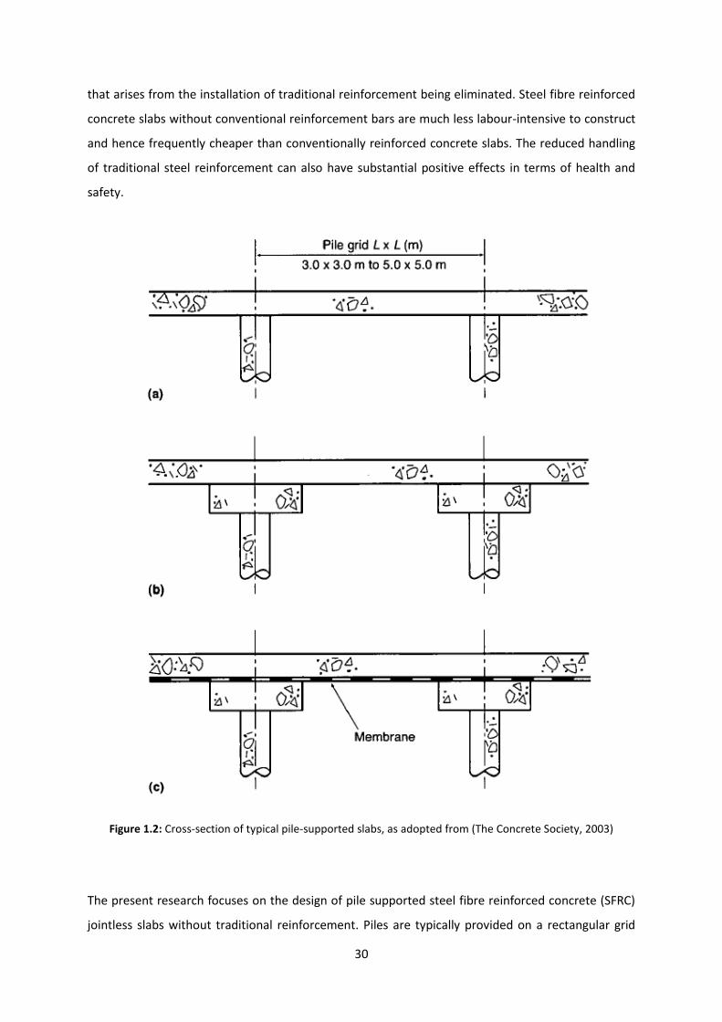
30
that arises from the installation of traditional reinforcement being eliminated. Steel fibre reinforced
concrete slabs without conventional reinforcement bars are much less labour-intensive to construct
and hence frequently cheaper than conventionally reinforced concrete slabs. The reduced handling
of traditional steel reinforcement can also have substantial positive effects in terms of health and
safety.
Figure 1.2: Cross-section of typical pile-supported slabs, as adopted from (The Concrete Society, 2003)
The present research focuses on the design of pile supported steel fibre reinforced concrete (SFRC)
jointless slabs without traditional reinforcement. Piles are typically provided on a rectangular grid
31
with spacings of 3m to 5m. The slab thickness is typically selected on the basis of a span to depth
ratio of 15 with a minimum slab thickness of 200mm (The Concrete Society, 2012). Previous case
studies show that typical steel fibre dosages lie between 35 – 50 kg/m3 (Hedebratt & Silfwerbrand,
2004) (The Concrete Society, 2007). Cracking can arise in pile supported slabs due to the combined
effects of restrained shrinkage and imposed loading. Cracking due to restraint is typically minimised
by casting the slab onto a polythene membrane to minimise frictional restraint (1.2(c)). Additionally,
piles are not built into slabs to minimise lateral restraint from the piles. The soil is assumed to
provide temporary support during the construction of the slab but not subsequently when the slab is
assumed to be fully supported by the piles (The Concrete Society, 2012).
Due to the absence of codified or authoritative guidance, SFRC pile supported slabs are frequently
designed using proprietary methods. Although SFRC has been in use for a number of years, there is
little agreement on the design principles that should be adopted (The Concrete Society, 2007). At
present, a wide variety of test methods involving beam and plate tests are used in industry to
determine the material properties and structural response of SFRC. The present work aims to
compare the properties derived from the beam and round plate tests and relate these to the design
of SFRC pile supported slabs.
The key design concerns are the flexural and punching shear resistances at the ultimate limit state
and cracking at the serviceability limit state. The yield line method is widely used for the design of
pile supported slabs at the ultimate limit state. However, there is a lack of agreement on the
moment of resistance that should be used in design. The applicability of the yield line method for
the design of SFRC pile supported slabs is considered within the present thesis.
The enhancement in the punching shear resistance of slabs provided by the addition of the steel
fibres has been researched (Swamy & Ali, 1982) (Alexander & Simmonds, 1992) (Labib, 2008).
However, due to a lack of test data, there is a lack of codified guidance on the determination of the
punching shear resistance of SFRC slabs without conventional reinforcement. Consequently, a series
of tests were carried out to determine the punching shear resistance of SFRC in the absence of
conventional reinforcement.
At the serviceability limit state, a key objective is to minimise cracking. Cracking due to imposed
loading is most likely to occur over piles and under point loads where flexural stresses are greatest.
Pile supported slabs are commonly used in industrial warehouses where any cracking can result in
impaired performance. Although, extensive cracking does not necessarily result in catastrophic
failure, the financial repercussions can be severe as the slab becomes unserviceable. Currently, very

32
little guidance is available on the calculation of crack widths in SFRC slabs without conventional
reinforcement. This thesis examines the feasibility of relating the crack widths in SFRC slabs to the
imposed deformation.
Figure 1.3: Typical steel fibres used in industrial applications, such as the construction of pile-supported slabs
(adopted from http://www.mswukltd.co.uk/dramix_steelfibres.htm)
1.2 Objectives
The overall aim of the present research is to investigate the behaviour and design of steel-fibre
reinforced concrete pile-supported slabs. More specific objectives are:
To review current design provisions for the design of steel fibre reinforced pile-supported slabs
without traditional steel reinforcement.
To compare the flexural resistances given by notched beam and round plate tests.
To develop procedures for modelling pile-supported slabs in flexure using discrete and smeared
cracking approaches.
To investigate the applicability of yield line analysis to the design of SFRC slabs using design
orientated models and numerical modelling.
To develop improved design guidelines for steel fibre reinforced concrete slabs.
1.3 Research Methodology
To achieve the fore mentioned aims and objectives the following methodology has been devised:
To undertake a comprehensive review of relevant literature, in order to identify the state of the
art and unresolved issues, in the assessment and design of SFRC pile-supported slabs.
To review current design provisions for SFRC pile-supported slabs with emphasis on the residual
strength after cracking and serviceability issues such as cracking.

33
To identify, appropriate material models for simulating the structural behaviour of SFRC.
To undertake a program of structural tests to determine the material properties of SFRC.
To identify and use appropriate numerical models, to simulate the behaviour of pile-supported
slabs, including flexural failure, load-deflection behaviour, crack initiation and crack propagation
using the finite element method.
To relate crack widths to displacements in Round Determinate Panel (RDP) tests and continuous
slabs.
To examine the serviceability limit state performance of SFRC slabs designed with Yield Line
Analysis.
Evaluate the increase in punching shear resistance offered by the addition of steel fibres.
Make design recommendations for SFRC pile supported slabs.
1.4 Outline of Thesis
The present chapter provides a brief introduction into the design issues and constraints commonly
encountered in pile-supported slabs. The statement of the problem as well as the aims and the
objectives of the present research are defined.
Chapter Two presents a critical review of the state of the art. It examines the enhancement in
behaviour that is provided by the addition of steel fibres into the concrete mix with emphasis on the
post-peak response. A historical overview of the fracture mechanics concepts governing the
behaviour of SFRC is presented following the approach of Hillerborg et al. (1976). The stress – strain
(σ-ε), stress – crack width (σ-w) and crack band width approaches for numerical modelling are
critically reviewed. A critical assessment of the existing methods of determining the material
properties of SFRC, such as the EN 14651 notched beam and the ASTM beam and plate tests, is
undertaken.
Chapter Three describes current codified design provisions for SFRC pile-supported slabs. Possible
failure mechanisms in flexure and punching shear (ultimate limit state) are reviewed are also the
serviceability limit state issues governing the long-term performance such as shrinkage and cracking.
The shortcomings of the current design guidelines are discussed particularly with reference to the
determination of the crack widths in pile-supported slabs at the serviceability limit state.
Chapter Four describes the experimental programme carried out which included beam, RDP, slab
and punching shear tests. Details of the instrumentation, geometry and experimental procedure are

34
given for each of the above. Further details regarding the concrete mix, casting procedure and type
and dosages of fibres are also provided.
Chapter Five presents the results of the experimental programme described in Chapter Four. The
chapter begins with the EN 14651 beam test data. The discussion extends to the statically
determinate and indeterminate plate tests. Particular focus is given on the variability of the
performances encountered. This is followed by presentation of the additional plate and slab tests
undertaken with a particular focus on the additional crack width measurements obtained. A
discussion of the punching shear test results is also included.
Chapter Six describes the numerical modelling methodology adopted for the simulation of the
behaviour of SFRC pile-supported slabs. The chapter begins with a short introduction into the
application of the finite element method in structural engineering. This is followed by a brief
discussion of the smeared and discrete cracking approaches commonly associated with concrete
modelling. A review of the concrete constitutive models available with ABAQUS is given. The
proposed constitutive model is subsequently presented.
Chapter Seven presents the results of the Non Linear Finite Element Analysis (NLFEA). The chapter
begins with an introduction to the inverse analysis modelling procedure adopted for the
determination of a suitable stress – crack width (σ-w) response. This concept is extended to both the
EN 14651 beam tests and the RDP. The results obtained by both of these are subsequently analysed
and compared with the Yield Line Method. The moment and rotations along the Yield Line in the
RDP are examined. The experimental results are compared with the current design provisions
offered by the Technical report 34 and he Model Code 2010 (bulletin 66). The results of the slab
tests are analysed and compared with Yield Line and the present NLFEA.
Chapter Eight extends the NLFEA in the modelling of pile-supported slabs failing under flexure.
Particular focus is given on the moment along the Yield Line during the various stages of loading.
This is followed by a comparison of the discrete and the smeared cracking analysis methods.
Chapter Nine gives a summary of the present research project and the conclusions obtained from
the experiments and the NLFEA.

35
Chapter Two
Literature Review
2.1 Introduction
Concrete is intrinsically strong in compression but weak in tension. The traditional method of
overcoming this deficiency is to provide steel reinforcing bars to carry the tensile forces once the
concrete has cracked, or pre-stressing so that the majority of the concrete remains under
compression.
In many ground floor slabs for both commercial and industrial applications, only a nominal amount
of steel reinforcement is required to resist flexure and control cracking induced by the combined
effects of loading and restrained shrinkage. Alternatively, some or all of the conventional
reinforcement can be replaced with steel fibres.
Over the past few years, this concept has been largely adopted in many industrial and commercial
applications such as the construction of tunnel linings, pavements and ground floors. Nonetheless,
the wide application of steel fibres has not led to clear guidelines in regard to the behaviour and
design of such structures.
2.2 Historical Development of Steel Fibre Reinforced Concrete
2.2.1 Origin of Steel-Fibre Reinforced Concrete
The provision of fibrous materials to enhance the structural integrity of a brittle matrix is not an
entirely new notion. In fact, fibres have been utilised as reinforcement since ancient times. The use
of fibre-reinforced composites, such as mud bricks reinforced with straws or mortar reinforced with
horsehair can be traced back to ancient Egypt, some 2500 years ago (Illston & Domone, 2004).
At the turn of the 20th century, asbestos fibres were commonly incorporated in concrete
construction. Experimentation involving the use of steel fibres can be traced back as early as 1910 by
Porter (1910). Both the compressive and tensile strength of the concrete were found to be increased
significantly from the inclusion of short pieces of steel. Within the same publication (Porter, 1910) it

36
was also foreseen that such reinforcement would be widely implemented in many structural
applications.
Four years later, the first patent was taken out by W. Ficklen. The patent stated the inclusion of
small metal segments impregnated within the concrete mix in order to increase its fracture
toughness (Ficklen, 1914).
Very modest advances were made in the technology of composite materials until the early 1950s. At
that time the health risks associated with the asbestos fibres, which had become a very common
building material, were discovered. This triggered a substantial amount of research into alternative
forms of construction, one of them being steel-fibre reinforced concrete.
2.2.2 Historical Development
The first meaningful contribution to fibre strengthening mechanics was made by Romualdi et al.
(1963) in the early 1960s. Romualdi et al. (1963) postulated a fracture mechanics approach for the
derivation of the cracking strength of mortar reinforced with closely spaced steel fibres. This was the
first attempt to develop a framework to describe the constitutive behaviour of a fibre reinforced
composite.
In 1974, Swamy et al. proposed a constitutive relationship for the estimation of the flexural strength
of steel fibre reinforced concrete. Within the context of this publication, it was argued that the
interfacial bond stress between the brittle matrix and its fibrous components was largely linear. A
reasonable correspondence with the proposed relationship and previous experimental data was
attained.
Unfortunately, the above framework only applied to composites with the ability to sustain additional
load after the formation of the first crack, also termed tension hardening behaviour (Lim,
Paramasivam, & Lee, 1987). Addressing this issue, Lim et al. (1987) formulated an analytical model to
describe the tensile behaviour of steel fibre reinforced concrete, simulating both tension hardening
and tension softening behaviour.
The increasing demand of the construction industry for alternative construction methods has led to
the development and implementation of Steel Fibre Reinforced Concrete (SFRC) in a wide variety of
both industrial and commercial applications. Such applications include the design and construction
of pile-supported and ground-supported floor slabs, pavements and tunnel linings. This has triggered
considerable developments, in more recent years, in SFRC constitutive modelling (Hillerborg, 1980)
(Barros & Figueiras, 1999) (Bernard & Pircher, 2000) (RILEM Technical Committee, 2002)
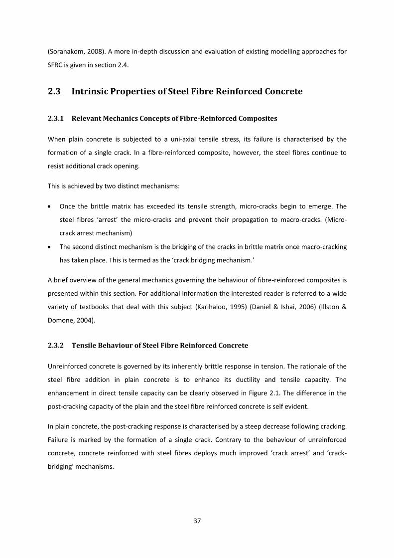
37
(Soranakom, 2008). A more in-depth discussion and evaluation of existing modelling approaches for
SFRC is given in section 2.4.
2.3 Intrinsic Properties of Steel Fibre Reinforced Concrete
2.3.1 Relevant Mechanics Concepts of Fibre-Reinforced Composites
When plain concrete is subjected to a uni-axial tensile stress, its failure is characterised by the
formation of a single crack. In a fibre-reinforced composite, however, the steel fibres continue to
resist additional crack opening.
This is achieved by two distinct mechanisms:
Once the brittle matrix has exceeded its tensile strength, micro-cracks begin to emerge. The
steel fibres ‘arrest’ the micro-cracks and prevent their propagation to macro-cracks. (Micro-
crack arrest mechanism)
The second distinct mechanism is the bridging of the cracks in brittle matrix once macro-cracking
has taken place. This is termed as the ‘crack bridging mechanism.’
A brief overview of the general mechanics governing the behaviour of fibre-reinforced composites is
presented within this section. For additional information the interested reader is referred to a wide
variety of textbooks that deal with this subject (Karihaloo, 1995) (Daniel & Ishai, 2006) (Illston &
Domone, 2004).
2.3.2 Tensile Behaviour of Steel Fibre Reinforced Concrete
Unreinforced concrete is governed by its inherently brittle response in tension. The rationale of the
steel fibre addition in plain concrete is to enhance its ductility and tensile capacity. The
enhancement in direct tensile capacity can be clearly observed in Figure 2.1. The difference in the
post-cracking capacity of the plain and the steel fibre reinforced concrete is self evident.
In plain concrete, the post-cracking response is characterised by a steep decrease following cracking.
Failure is marked by the formation of a single crack. Contrary to the behaviour of unreinforced
concrete, concrete reinforced with steel fibres deploys much improved ‘crack arrest’ and ‘crack-
bridging’ mechanisms.

38
Figure 2.1: Schematic depiction of tensile response for different dosages of steel fibres (from Maild, 2005 as
cited in Kooiman, 2000)
The tensile response of a steel fibre reinforced composite can generally be sub-divided into three
distinct phases:
Elastic phase
Micro-cracking phase
Fibre pull out and failure (macro-cracking) phase
Elastic Phase
The elastic phase characterises the response of the SFRC prior to crack formation. The elastic
modulus and the ultimate tensile strength of the composite can be derived from the following
equations (Daniel & Ishai, 2006):
mmffoc VEVEE (2.1)
m
ff
ofmcE
EVVff 1 (2.2)
where, o and are orientation and length effectiveness coefficients of the steel fibres respectively,
fE and mE denote the elastic moduli of the steel fibres and the concrete matrix, fV and mV indicate
the volume of the fibres and the matrix, whereas mf denotes the tensile strength of the matrix.
Micro-cracking Phase
This stage is characterised by the exceeding of the tensile strength of the concrete matrix and the
formation of the first micro-cracks. At the cracks, the load carried by the concrete is transferred to

39
the steel fibres. The fibres intersecting a crack will resist additional crack opening via the crack arrest
and crack bridging mechanisms, as defined in section 2.3.1.
If the fibres cannot resist additional stress after the initial crack formation, then the behaviour of the
composite is governed by a single crack (RILEM Technical Committee, 2002). This response is termed
tension softening.
In contrast, when the fibres can resist additional stress after the initial crack formation, then the
behaviour is characterised by a multiple crack formation. This is also known as a strain hardening
(pseudo-strain) response.
Fibre Pull-Out and Failure (Macro-cracking) Phase
The fibre pullout and macro-cracking phase is the final stage of the tensile response of a steel fibre
reinforced composite. If the failure is governed by gradual pull-out of the fibres, then a ductile
response can be observed. In contrast, if the failure is primarily governed by fracture of the fibres
themselves, then a brittle response occurs.
The post-cracking response is influenced by the bond stresses at the matrix-fibre interface, the
dosage of fibre (as demonstrated in Figure 2.1), the fibre type (straight, crimped, hooked-end) as
well as the fibre dosage.
2.3.3 Compressive Behaviour of Steel Fibre Reinforced Concrete
Steel fibres have a much smaller impact on the compressive response of Steel Fibre Reinforced
Concrete, than its tensile response. Research has shown that there is a small decrease in the Elastic
Modulus of the concrete when steel fibres are added to the matrix (Neves et al., 2005). This fact is
attributed to the small voids introduced from the addition of the steel fibres.
However, the steel fibres introduce additional ductility in the overall compressive response
(Kooiman, van der Veen, & Walraven, 2000) (Lim & Nawy, 2005). This can prove beneficial in the
case of a compressive failure (Barros & Figueiras, 1999) (Labib, 2008). Both of these effects are
demonstrated graphically in Figure 2.2:
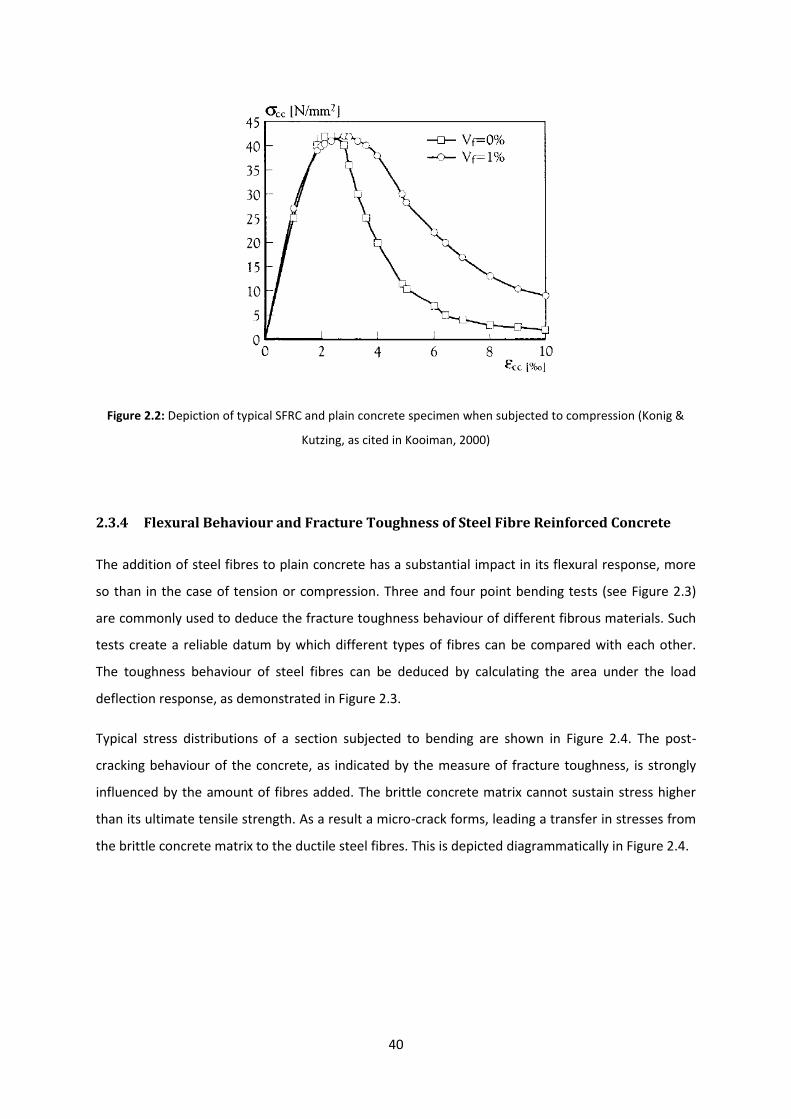
40
Figure 2.2: Depiction of typical SFRC and plain concrete specimen when subjected to compression (Konig &
Kutzing, as cited in Kooiman, 2000)
2.3.4 Flexural Behaviour and Fracture Toughness of Steel Fibre Reinforced Concrete
The addition of steel fibres to plain concrete has a substantial impact in its flexural response, more
so than in the case of tension or compression. Three and four point bending tests (see Figure 2.3)
are commonly used to deduce the fracture toughness behaviour of different fibrous materials. Such
tests create a reliable datum by which different types of fibres can be compared with each other.
The toughness behaviour of steel fibres can be deduced by calculating the area under the load
deflection response, as demonstrated in Figure 2.3.
Typical stress distributions of a section subjected to bending are shown in Figure 2.4. The post-
cracking behaviour of the concrete, as indicated by the measure of fracture toughness, is strongly
influenced by the amount of fibres added. The brittle concrete matrix cannot sustain stress higher
than its ultimate tensile strength. As a result a micro-crack forms, leading a transfer in stresses from
the brittle concrete matrix to the ductile steel fibres. This is depicted diagrammatically in Figure 2.4.
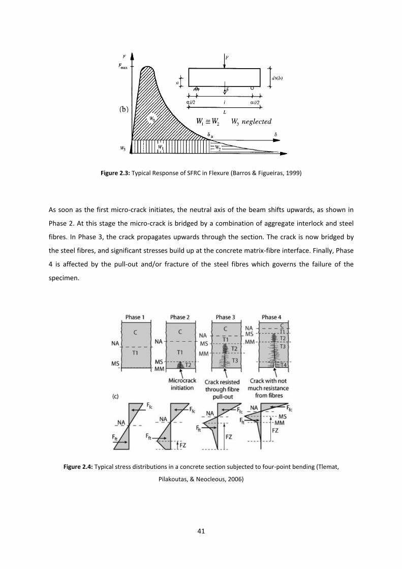
41
Figure 2.3: Typical Response of SFRC in Flexure (Barros & Figueiras, 1999)
As soon as the first micro-crack initiates, the neutral axis of the beam shifts upwards, as shown in
Phase 2. At this stage the micro-crack is bridged by a combination of aggregate interlock and steel
fibres. In Phase 3, the crack propagates upwards through the section. The crack is now bridged by
the steel fibres, and significant stresses build up at the concrete matrix-fibre interface. Finally, Phase
4 is affected by the pull-out and/or fracture of the steel fibres which governs the failure of the
specimen.
Figure 2.4: Typical stress distributions in a concrete section subjected to four-point bending (Tlemat,
Pilakoutas, & Neocleous, 2006)
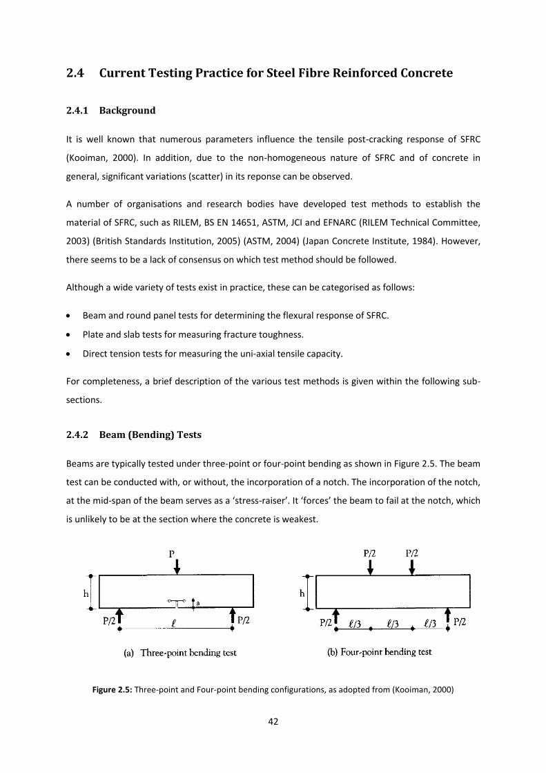
42
2.4 Current Testing Practice for Steel Fibre Reinforced Concrete
2.4.1 Background
It is well known that numerous parameters influence the tensile post-cracking response of SFRC
(Kooiman, 2000). In addition, due to the non-homogeneous nature of SFRC and of concrete in
general, significant variations (scatter) in its reponse can be observed.
A number of organisations and research bodies have developed test methods to establish the
material of SFRC, such as RILEM, BS EN 14651, ASTM, JCI and EFNARC (RILEM Technical Committee,
2003) (British Standards Institution, 2005) (ASTM, 2004) (Japan Concrete Institute, 1984). However,
there seems to be a lack of consensus on which test method should be followed.
Although a wide variety of tests exist in practice, these can be categorised as follows:
Beam and round panel tests for determining the flexural response of SFRC.
Plate and slab tests for measuring fracture toughness.
Direct tension tests for measuring the uni-axial tensile capacity.
For completeness, a brief description of the various test methods is given within the following sub-
sections.
2.4.2 Beam (Bending) Tests
Beams are typically tested under three-point or four-point bending as shown in Figure 2.5. The beam
test can be conducted with, or without, the incorporation of a notch. The incorporation of the notch,
at the mid-span of the beam serves as a ‘stress-raiser’. It ‘forces’ the beam to fail at the notch, which
is unlikely to be at the section where the concrete is weakest.
Figure 2.5: Three-point and Four-point bending configurations, as adopted from (Kooiman, 2000)
43
A number of bending test methods have been proposed for use in the design of SFRC. The most
important of these are explained within the next few sub-sections. Of these, the Japanese beam test
(Japan Concrete Institute, 1984) was commonly used in the UK before the introduction of the EN
14651 test method, which is based on the RILEM beam test (RILEM Technical Committee, 2000).
JCI-SF4
The JCI-SF4 beam test (Japan Concrete Institute, 1984) was used in the UK before it was superseded
by the notched beam test of BS EN 14651. A minimum of six beam bending tests of dimensions 150 x
150 x 600mm with a span of 450mm under four point bending must be executed according to the
recommendations of the JCI.
The computation of the equivalent flexural strength involves the determination of the fracture
toughness up to a pre-determined deflection of 3mm at the centre of the beam. The equivalent
flexural strength is evaluated with the following expression:
, ,3 2150
JCLct fleq
T Lf
bh (2.3)
where, JCLT is the fracture toughness up to a deflection of 3mm; L is the length of the specimen;
150 = span/150 = 3mm;b is the beam width and h denotes the depth of the specimen.
The test results are only valid upon the initiation of a single crack in the middle third of the beam
(Japan Concrete Institute, 1984) which can lead to some tests being discarded. In addition, the load
and the crack width are arbitrarily related since the position of the crack varies with the position of
the weakest section within the central third of the beam. Therefore, the crack width corresponding
to a particular deflection depends on the position of the crack. The fact that the crack could in
theory occur anywhere along the beam also makes it difficult to measure crack widths.
In light of the constraints presented by the JCI-SF4, BS EN 14651:2005 adopted the
recommendations of the RILEM Technical committee. Consequently, the use of JCI-SF4 has been
superseded in the UK by BS EN 14651:2005.
RILEM TC-162 TDF
RILEM recently proposed a standard three-point bending configuration for the evaluation of the
flexural performance of SFRC (RILEM Technical Committee, 2002). The RILEM beam-bending test
incorporates a notch in order to predetermine the failure mode of the specimen. This is done so that
the Crack Mouth Opening Displacement (CMOD) can also be measured during the test.

44
According to the RILEM Recommendations, test specimens with a square cross section of 150mm x
150mm should be used, with a minimum total length of 550mm encompassing a span length of
500mm and a notch of 25mm (RILEM, 2000).
This method uses the concept of the Limit of Proportionality (LOP). The LOP is defined as the highest
flexural stress within the interval of 0.05mm (RILEM, 2000). It is a function of the flexural strength
and is defined by the following expression:
, 2
3
2
ufct fl
sp
F Lf
bh (2.4)
where, uF is the load at the limit of proportionality, L is the span of the specimen, whereasb and sph
are the beam width and the height above the notch of the beam respectively.
By making use of the fracture toughness values, as defined in Figure 2.6, one can determine the
equivalent tensile strength by the use of the following empirical equations (RILEM, 2000).
Figure 2.6: Definition of fracture toughness values Df,2 and Df,3 , adapted from (RILEM, 2000) as cited in
(Kooiman, 2000)
,2, ,2,
,2 2
3
2 0.65 0.50
f I f II
eq
sp
D D Lf
bh
(2.5)
,3, ,3,
,3 2
3
2 2.65 2.50
f I f II
eq
sp
D D Lf
bh
(2.6)
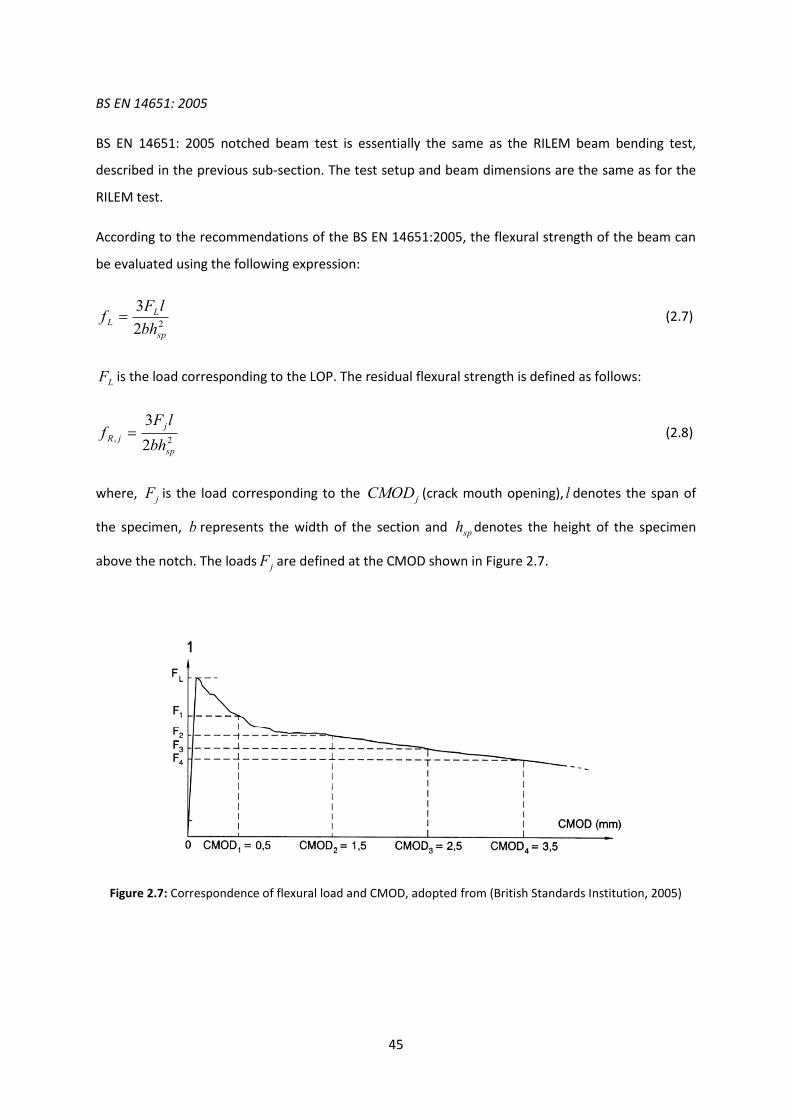
45
BS EN 14651: 2005
BS EN 14651: 2005 notched beam test is essentially the same as the RILEM beam bending test,
described in the previous sub-section. The test setup and beam dimensions are the same as for the
RILEM test.
According to the recommendations of the BS EN 14651:2005, the flexural strength of the beam can
be evaluated using the following expression:
22
3
sp
LL
bh
lFf (2.7)
LF is the load corresponding to the LOP. The residual flexural strength is defined as follows:
2,2
3
sp
j
jRbh
lFf (2.8)
where, jF is the load corresponding to the jCMOD (crack mouth opening), l denotes the span of
the specimen, b represents the width of the section and sph denotes the height of the specimen
above the notch. The loads jF are defined at the CMOD shown in Figure 2.7.
Figure 2.7: Correspondence of flexural load and CMOD, adopted from (British Standards Institution, 2005)

46
ASTM Beam Test C1399
The ASTM beam test uses a four-point bending configuration, unlike the RILEM and EN 14651 beam
bending tests. ASTM C1399 (2004) specifies specimens of 100 x 100 x 350mm with a span of 300mm
under four point bending. The distance between the two loads is 100mm.
The beam is initially loaded up to a deflection of 0.5mm. Then the load is slowly relieved and the
beam is re-loaded again (American Society for Testing and Materials , 2004). The residual strength is
determined from averaging the loads at four pre-determined deflections of 0.5mm, 0.75mm, 1.0mm
and 1.25mm. The toughness can then be measured from the load under the curve up to a deflection
of 0.5mm.
The geometry (length and width) of the crack obtained before the release of the load can vary
between different specimens. Like JCI, the load and the crack width are not directly related, as the
position of the crack can vary.
ASTM Beam Test C1609
ASTM C1609 (2005) uses 150mm x 150mm x 350mm beams tested under four point loading over a
span of 300mm. The difference between the present standard and the C1399 is that the loading is
continuous.
The fact that the loading is continuous allows the recording of the response of the fibres
immediately after the first crack. This is a critical point in assessing the ductility offered by the fibres
as opposed to plain concrete. The fact that the crack width cannot be recorded is still a major
drawback, particularly as steel fibres are typically used for crack control.
Model Code 2010
Model Code (MC 2010) adopts the BS EN 14651:2005 beam test.
The residual flexural strength as well as the LOP of a three point bending notched beam is calculated
using equation 2.4 as per the BS EN 14651:2005 recommendations. The moment of resistance uM of
a section is defined as follows:
26
22
3 spFTuspR
u
bhfbhfM (2.9)
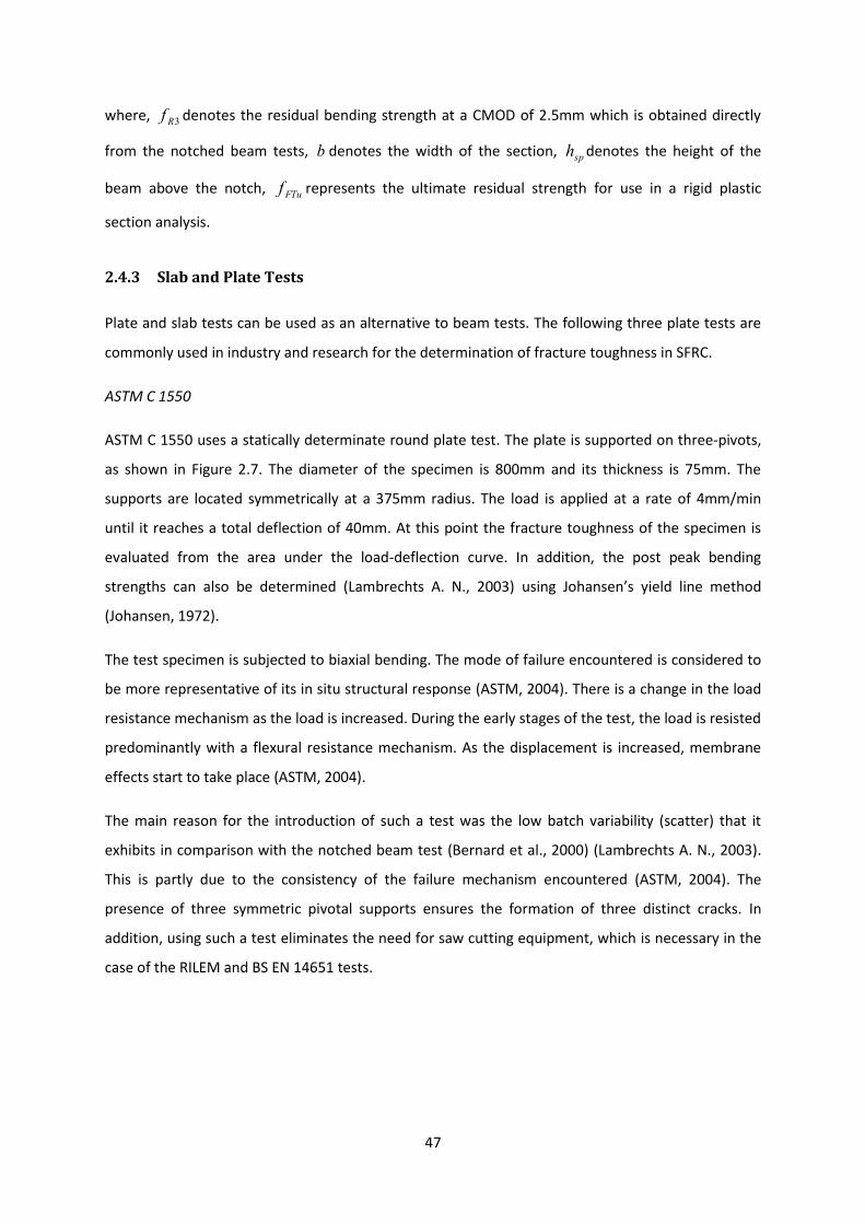
47
where, 3Rf denotes the residual bending strength at a CMOD of 2.5mm which is obtained directly
from the notched beam tests, b denotes the width of the section, sph denotes the height of the
beam above the notch, FTuf represents the ultimate residual strength for use in a rigid plastic
section analysis.
2.4.3 Slab and Plate Tests
Plate and slab tests can be used as an alternative to beam tests. The following three plate tests are
commonly used in industry and research for the determination of fracture toughness in SFRC.
ASTM C 1550
ASTM C 1550 uses a statically determinate round plate test. The plate is supported on three-pivots,
as shown in Figure 2.7. The diameter of the specimen is 800mm and its thickness is 75mm. The
supports are located symmetrically at a 375mm radius. The load is applied at a rate of 4mm/min
until it reaches a total deflection of 40mm. At this point the fracture toughness of the specimen is
evaluated from the area under the load-deflection curve. In addition, the post peak bending
strengths can also be determined (Lambrechts A. N., 2003) using Johansen’s yield line method
(Johansen, 1972).
The test specimen is subjected to biaxial bending. The mode of failure encountered is considered to
be more representative of its in situ structural response (ASTM, 2004). There is a change in the load
resistance mechanism as the load is increased. During the early stages of the test, the load is resisted
predominantly with a flexural resistance mechanism. As the displacement is increased, membrane
effects start to take place (ASTM, 2004).
The main reason for the introduction of such a test was the low batch variability (scatter) that it
exhibits in comparison with the notched beam test (Bernard et al., 2000) (Lambrechts A. N., 2003).
This is partly due to the consistency of the failure mechanism encountered (ASTM, 2004). The
presence of three symmetric pivotal supports ensures the formation of three distinct cracks. In
addition, using such a test eliminates the need for saw cutting equipment, which is necessary in the
case of the RILEM and BS EN 14651 tests.

48
Figure 2.8: Schematic Illustration of the ASTM C 1550 statically determinate round panel test, as adopted from
(Bernard, 2005)
EFNARC
The EFNARC tests were proposed mainly for use with sprayed concrete. Unlike the ASTM C 1550, a
square panel, rather than a circular plate, is used with dimensions of 600 x 600 x 100mm. The panel
is supported on each side, with a clear span of 500mm. This test falls under the category of
indeterminate panel tests.
The fracture toughness is then evaluated by measuring the area under the load-deflection curve up
to a central deflection of 25mm. One of the major drawbacks of this test is the unpredictability of
the crack pattern (Lambrechts A. N., 2007) particularly after the addition of the fibres into the mix.
The fibres provide an improved crack arrest mechanism combined with the ability to re-distribute
moments after cracking.
BS EN 14488 Plate Test
BS EN 14488 adopts the recommendation of the EFNARC panel test, as described in the previous
sub-section.
49
Other Plate Tests
In the case of pile-supported slabs it is commonplace to use tests that are claimed to better simulate
service conditions. A number of fibre suppliers utilise non-standard statically indeterminate plate
tests as part of their design process. At present, design based on testing indeterminate round plates
is not a generally accepted test method (The Concrete Society, 2007).
2.4.4 Critical Assessment of Testing Methods
Having presented a brief overview of some common beam and plate test methods, this section
critically reviews these test methods. Emphasis is placed on the development of design guidelines
for SFRC pile-supported slabs.
Beam Tests
The prime benefit of beam tests is that they give material properties (Sukontasukkul, 2003). The test
however suffers from the disadvantage that the results can exhibit considerable scatter. However
there is a widespread belief, amongst many steel fibre suppliers that beam tests do not model
accurately the response of pile-supported slabs (Concrete society, 2007). The main reasoning behind
this argument is the fact that simply supported beams do not exhibit the load re-distribution that
occurs in pile-supported slabs on cracking. As a result the post-peak response does not correspond
with that of a statically indeterminate pile-supported slab (Destree, 2004). After the initiation of the
crack in the beam test, a drop in flexural load is typical of a tension softening response. On the other
hand, pile-supported slabs do not necessarily behave in such fashion as they are statically
indeterminate. Consequently, a re-distribution of stresses occurs within the slab after initial cracking
(Lambrechts A. N., 2007) which can result in an initially hardening response. The redistribution of
stresses can occur from adjacent bays or piles.
The counter argument is that the beam tests give material properties whereas indeterminate plate
tests give the structural response. Hypothetically, the structural response of the statically
indeterminate test, or the pile supported slab, should be predictable once the relevant material
properties are known.
The previous sub-sections described various standard beam tests in which variations included both
the loading arrangement (three point bending – RILEM, BS EN 14651, four point bending – ASTM
C1399, C1609) and loading method (continuous – RILEM, BS EN 14651, non-continuous – ASTM
C1399). Each test exhibits its own distinct benefits and drawbacks as described below.
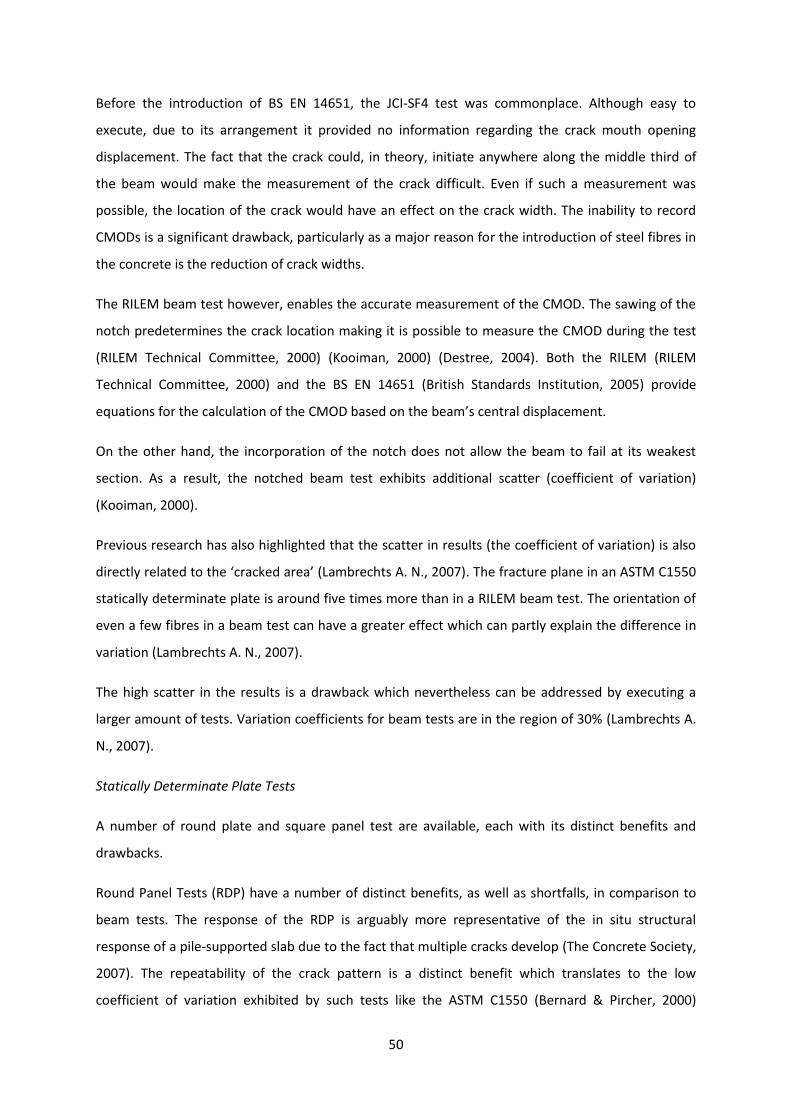
50
Before the introduction of BS EN 14651, the JCI-SF4 test was commonplace. Although easy to
execute, due to its arrangement it provided no information regarding the crack mouth opening
displacement. The fact that the crack could, in theory, initiate anywhere along the middle third of
the beam would make the measurement of the crack difficult. Even if such a measurement was
possible, the location of the crack would have an effect on the crack width. The inability to record
CMODs is a significant drawback, particularly as a major reason for the introduction of steel fibres in
the concrete is the reduction of crack widths.
The RILEM beam test however, enables the accurate measurement of the CMOD. The sawing of the
notch predetermines the crack location making it is possible to measure the CMOD during the test
(RILEM Technical Committee, 2000) (Kooiman, 2000) (Destree, 2004). Both the RILEM (RILEM
Technical Committee, 2000) and the BS EN 14651 (British Standards Institution, 2005) provide
equations for the calculation of the CMOD based on the beam’s central displacement.
On the other hand, the incorporation of the notch does not allow the beam to fail at its weakest
section. As a result, the notched beam test exhibits additional scatter (coefficient of variation)
(Kooiman, 2000).
Previous research has also highlighted that the scatter in results (the coefficient of variation) is also
directly related to the ‘cracked area’ (Lambrechts A. N., 2007). The fracture plane in an ASTM C1550
statically determinate plate is around five times more than in a RILEM beam test. The orientation of
even a few fibres in a beam test can have a greater effect which can partly explain the difference in
variation (Lambrechts A. N., 2007).
The high scatter in the results is a drawback which nevertheless can be addressed by executing a
larger amount of tests. Variation coefficients for beam tests are in the region of 30% (Lambrechts A.
N., 2007).
Statically Determinate Plate Tests
A number of round plate and square panel test are available, each with its distinct benefits and
drawbacks.
Round Panel Tests (RDP) have a number of distinct benefits, as well as shortfalls, in comparison to
beam tests. The response of the RDP is arguably more representative of the in situ structural
response of a pile-supported slab due to the fact that multiple cracks develop (The Concrete Society,
2007). The repeatability of the crack pattern is a distinct benefit which translates to the low
coefficient of variation exhibited by such tests like the ASTM C1550 (Bernard & Pircher, 2000)

51
(Lambrechts A. N., 2003) (Marti, Pfyl, Sigrist, & Ulaga, 1999). According to Lambrecht (2007) ‘the
average variation coefficient is around 10%’. This is approximately a third of the variation of
coefficient for standard beam tests.
Previous research has demonstrated that the influence of the location of the three radial cracks has
a very small effect on the load resistance of the plate (Bernard & Xu, 2008).
As plate tests generate a larger number of cracks, they are able to absorb more fracture energy than
beams (Sukontasukkul, 2003). That can enable the fibres to demonstrate their ability in bridging a
crack. A few researchers categorise the RDP test as a more logical choice for the determination of
the fracture toughness of SFRC (Banthia, Gupta, & Yan, Impact Resistance of Fibre Reinforced Wet-
Mix Shotcrete-Part 2: Plate Tests, 1999) (Sukontasukkul, 2003).
The ASTM C1550 is a RDP which has been designed for easy fabrication as well as execution (Bernard
& Pircher, 2000). The three pivotal points ensure that the test is always in conctact with the support
regardless of the flatness of the specimen itself.
The limitation of this test is that it is not easy to record the crack width. The fact that the crack width
tends to vary along the yield lines makes such a calculation even more difficult.
Statically Indeterminate Plate Tests
Whereas the statically determinate tests (beam tests and round determinate round panels) help to
extract material properties, tests of statically indeterminate nature (Arcelor plate test, EN 14488,
EFNARC panel test) are predominately used to understand the structural behaviour of SFRC with
regard to specific applications (Lambrechts A. N., 2007).
Their statically indeterminate nature makes it difficult to extract the intrinsic material properties of
the SFRC. Primarily, this is due to the fact that the stress distribution is not known and cannot be
derived due to the indeterminate boundary conditions. Such tests do not exhibit a consistent mode
of failure as in the case of the RDP (Bernard, 2000). The cracking pattern observed can also be
unpredictable, particularly in the case of the square panel specimens, postulated in EN 14488-5. The
addition of the fibres into the mix can make the crack pattern even less predictable given the ability
of the fibres to transfer stresses across the concrete matrix after fracture has initiated (Lambrechts
A. N., 2007).
A distinct advantage of the RDP over the ENFRAC test is the even load distribution. The three
symmetric pivotal supports ensure an even load distribution ‘regardless of tolerances’ and surface
flatness (Bernard & Pircher, 2000). Furthermore, the flexural resistance of such tests is not directly

52
related to the crack-width (Concrete Society, 2007). This is due to the known fact that the flexural
resistance tends to vary along the yield lines as the CMOD is not known.
For this reason, it can be argued that indeterminate plate and slab tests should not be used to
measure the material properties but rather to monitor the overall structural response.
2.5 Constitutive Behaviour of Steel Fibre Reinforced Concrete
2.5.1 Introduction to SFRC Constitutive Modelling and Research Background
The benefits introduced by the incorporation of SFRC have led to a dramatic increase in usage in a
multitude of practical applications. This posed a research challenge to introduce and generate a
constitutive model to imitate the structural behaviour of SFRC.
A large number of constitutive models have been developed for SFRC (Romualdi & Batson, 1963)
(Hillerborg, 1980) (Lim, Paramasivam, & Lee, 1987) (Barros & Figueiras, 1999) (Olesen, 2001) (RILEM
Technical Committee, 2002) (RILEM Technical Committee, 2003), all encompassing different
research philosophies. The various constitutive models can be categorised, according to their
philosophy, as follows:
Stress-crack width
Stress-strain
Crack band width philosophy
The following sections examine these three approaches in detail. Each modelling philosophy is
described and analysed in detail. This analysis forms a stepping stone to the modelling approach
selected in the present work.
2.5.2 Stress-Crack Width Philosophy
The primary constitutive modelling philosophy that will be described within the context of the
present chapter is the stress-crack width approach.
The promulgation of a crack through plain concrete can be represented by a region of micro-cracking
incorporating a ‘process zone and a localized crack’ (Hillerborg et al., 1976) (RILEM Technical
Committee, 2002). In turn, the localised crack zone is sub-divided into a traction free crack (also
termed as a macro-crack) and a zone where aggregate interlock occurs. This concept is
diagrammatically illustrated below (Figure 2.9).
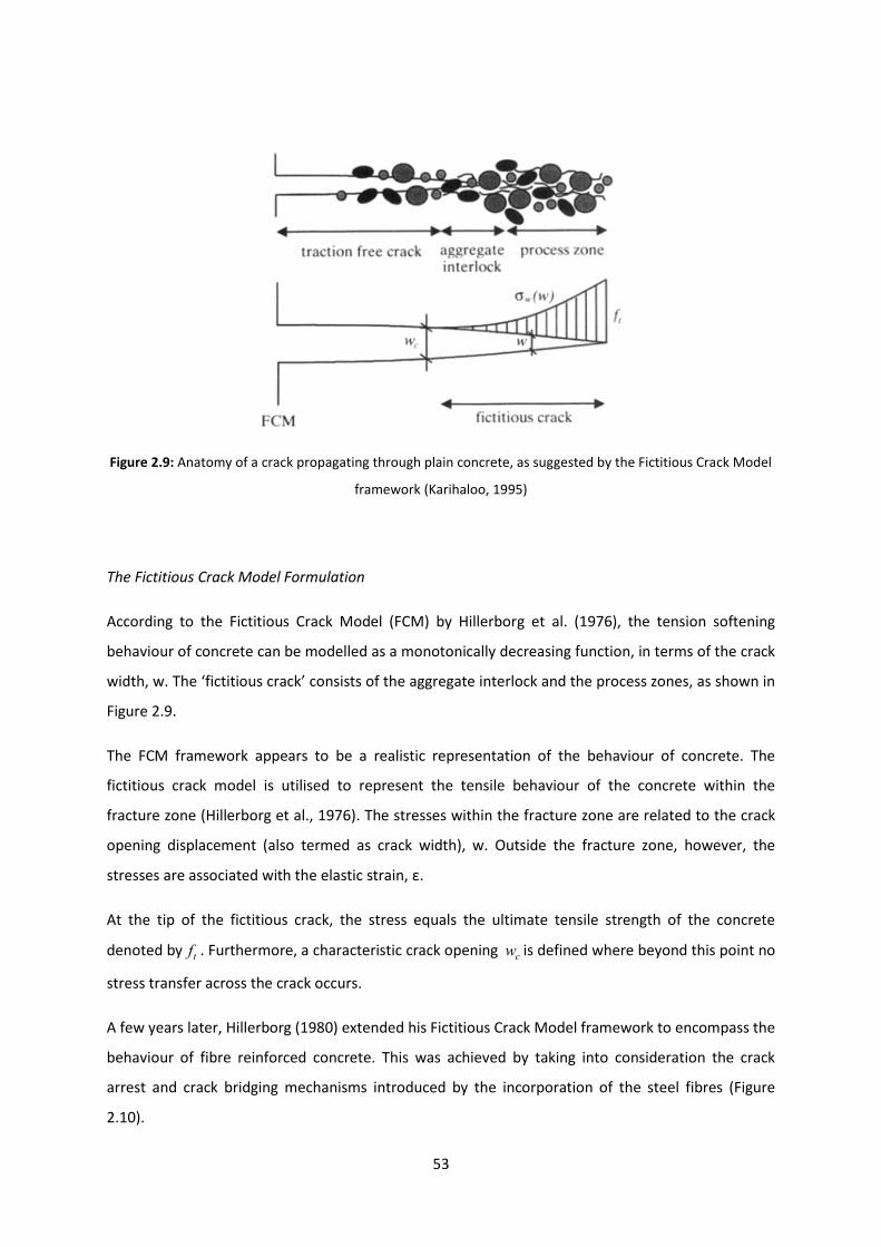
53
Figure 2.9: Anatomy of a crack propagating through plain concrete, as suggested by the Fictitious Crack Model
framework (Karihaloo, 1995)
The Fictitious Crack Model Formulation
According to the Fictitious Crack Model (FCM) by Hillerborg et al. (1976), the tension softening
behaviour of concrete can be modelled as a monotonically decreasing function, in terms of the crack
width, w. The ‘fictitious crack’ consists of the aggregate interlock and the process zones, as shown in
Figure 2.9.
The FCM framework appears to be a realistic representation of the behaviour of concrete. The
fictitious crack model is utilised to represent the tensile behaviour of the concrete within the
fracture zone (Hillerborg et al., 1976). The stresses within the fracture zone are related to the crack
opening displacement (also termed as crack width), w. Outside the fracture zone, however, the
stresses are associated with the elastic strain, ε.
At the tip of the fictitious crack, the stress equals the ultimate tensile strength of the concrete
denoted by tf . Furthermore, a characteristic crack opening cw is defined where beyond this point no
stress transfer across the crack occurs.
A few years later, Hillerborg (1980) extended his Fictitious Crack Model framework to encompass the
behaviour of fibre reinforced concrete. This was achieved by taking into consideration the crack
arrest and crack bridging mechanisms introduced by the incorporation of the steel fibres (Figure
2.10).
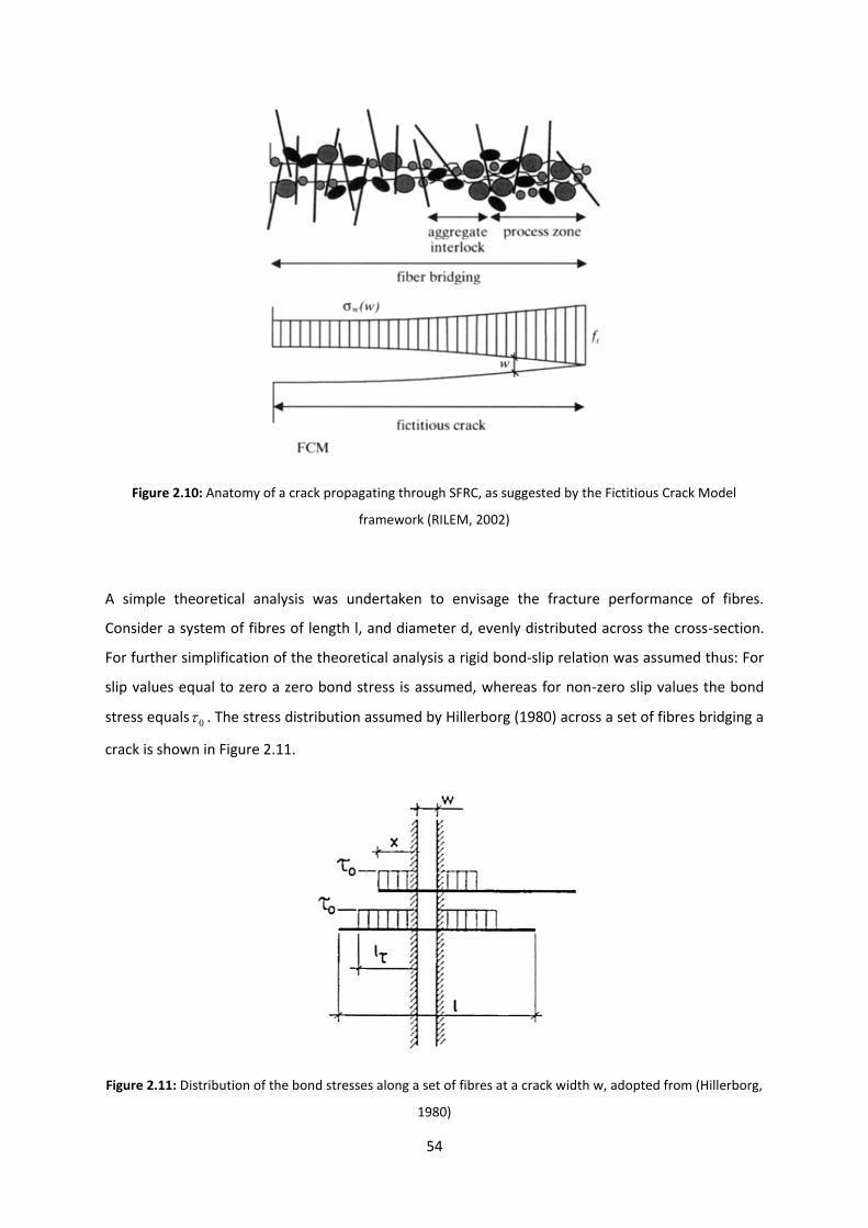
54
Figure 2.10: Anatomy of a crack propagating through SFRC, as suggested by the Fictitious Crack Model
framework (RILEM, 2002)
A simple theoretical analysis was undertaken to envisage the fracture performance of fibres.
Consider a system of fibres of length l, and diameter d, evenly distributed across the cross-section.
For further simplification of the theoretical analysis a rigid bond-slip relation was assumed thus: For
slip values equal to zero a zero bond stress is assumed, whereas for non-zero slip values the bond
stress equals 0 . The stress distribution assumed by Hillerborg (1980) across a set of fibres bridging a
crack is shown in Figure 2.11.
Figure 2.11: Distribution of the bond stresses along a set of fibres at a crack width w, adopted from (Hillerborg,
1980)

55
Hillerborg (1980) categorised the behaviour of fibres into two types: Fibres that encompass an
embedded length (on both sides) equal or greater than l , which are considered as fully anchored,
and fibres which the embedded length on one side is length than l .
For fully anchored fibres the tensile stress was derived, as follows:
04l
d
(2.10)
The crack width can then be formulated by multiplying the elastic extension and the embedded
length of the fibre between the points of zero slip:
w lE
(2.11)
On the other hand, the stress for fibres with an embedded length xwhich is less than l is described
by the following relationship:
04x
d (2.12)
Thus the mean stress carried by a fibre bridging the crack is given below:
04 1mean
l ll
d l l
(2.13)
In turn, the crack width can be described as a function of the bond stress, 0 and the critical fibre
length, l , thus:
22
04ll
wEd l
(2.14)
The Fictitious Crack Model (FCM) formulation has provided a significant framework to analyse the
crack formation and propagation in steel fibre reinforced concrete structures.
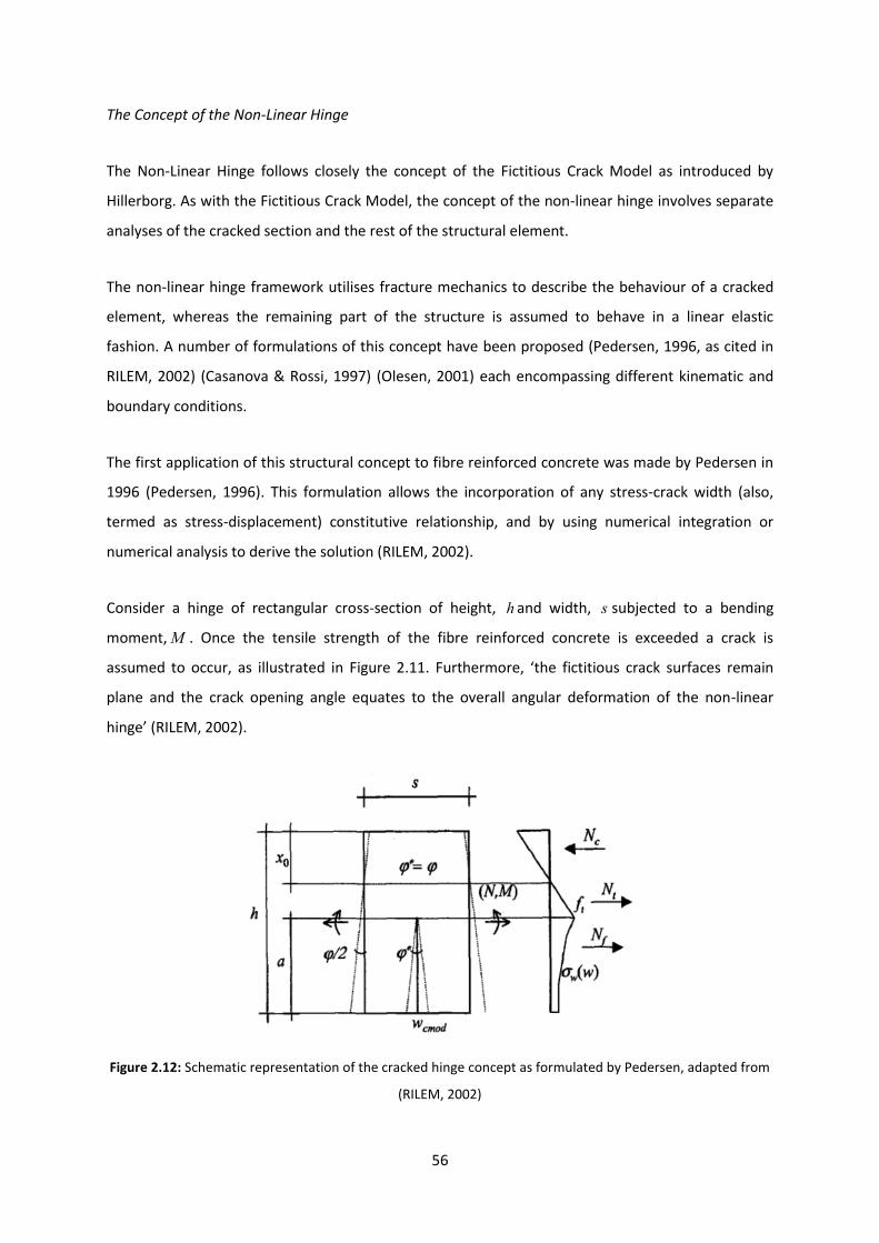
56
The Concept of the Non-Linear Hinge
The Non-Linear Hinge follows closely the concept of the Fictitious Crack Model as introduced by
Hillerborg. As with the Fictitious Crack Model, the concept of the non-linear hinge involves separate
analyses of the cracked section and the rest of the structural element.
The non-linear hinge framework utilises fracture mechanics to describe the behaviour of a cracked
element, whereas the remaining part of the structure is assumed to behave in a linear elastic
fashion. A number of formulations of this concept have been proposed (Pedersen, 1996, as cited in
RILEM, 2002) (Casanova & Rossi, 1997) (Olesen, 2001) each encompassing different kinematic and
boundary conditions.
The first application of this structural concept to fibre reinforced concrete was made by Pedersen in
1996 (Pedersen, 1996). This formulation allows the incorporation of any stress-crack width (also,
termed as stress-displacement) constitutive relationship, and by using numerical integration or
numerical analysis to derive the solution (RILEM, 2002).
Consider a hinge of rectangular cross-section of height, h and width, s subjected to a bending
moment,M . Once the tensile strength of the fibre reinforced concrete is exceeded a crack is
assumed to occur, as illustrated in Figure 2.11. Furthermore, ‘the fictitious crack surfaces remain
plane and the crack opening angle equates to the overall angular deformation of the non-linear
hinge’ (RILEM, 2002).
Figure 2.12: Schematic representation of the cracked hinge concept as formulated by Pedersen, adapted from
(RILEM, 2002)

57
As indicated in Figure 2.12, the shape of the crack as well as the crack boundary is assumed to
remain linear throughout the analysis. As a result, the following expression relating the crack width,
wwith the crack mouth opening angle * can be derived:
*w
a (2.15)
The tensile behaviour, within the SFRC cross-section is assumed to follow the stress-displacement
(crack-width) constitutive relation. Therefore both the bending moment and the axial force can be
deduced as a result of numerical integration as follows:
0
1
*
w
f wN u du
(2.16)
2 0
1
*
w
f wM u u du
(2.17)
As a result, the depth of the neutral axis denoted by 0h x , can then be determined by the following
relation:
0
1 tfh x s wE
(2.18)
In the above relation, s denotes the length of the non-linear hinge as indicated in Figure 2.12.
The axial force per unit width is split into two components: cN indicates the axial force per unit
width within the compression field, whereas tN indicates the axial force per unit width in the tensile
field of the section. The two components of the axial force can be described analytically by
equations (2.19) and (2.20):
20
2c
ExN
s
(2.19)
2
2
t
t
f sN
E (2.20)
Moreover, the moment of resistance can then be determined by taking moments about the neutral
axis of the section:
0 0 2
2 3 6 3 3 2c t f f
x xh h a hM N N a N M
(2.21)

58
Utilising the same logic, Casanova and Rossi (Casanova & Rossi, 1997) proposed an alternative
method of analysing SFRC sections. Although, like Pedersen (Pedersen, 1996), they assumed that
‘the fictitious crack surfaces remain plane and the crack deformation equates the overall angular
deformation of the non-linear hinge (Casanova & Rossi, 1997 as cited in RILEM, 2002), a parabolic
function of the curvature is used to define cracked mouth opening.
It is noteworthy, that the length of the non-linear hinge does not remain constant, but rather varies
with the crack length, a as follows:
2s a (2.22)
The crack mouth opening displacement can be computed using numerical integration using the
following constitutive relation:
21 222
3w a
(2.23)
where, 1 and 2 are the curvatures of the elastic and cracked parts of the hinge respectively, and
are defined by the following two expressions:
1 3
12M
Eh (2.24)
where M denotes the moment per unit width of the hinge .
2
0
c
x
(2.25)
where, c denotes the compressive strain and 0x denotes the neutral axis.
A few years later, Olesen (2001) suggested that the non-linear hinge could be modelled with
significant accuracy using ‘a layer of independent spring elements’ (Olesen, 2001). These elements
are divided into horizontal increments and are attached either side of the cracked boundary. This
concept is illustrated diagrammatically in Figure 2.13.
Consequently, the mean curvature, * and the longitudinal strain, * are defined by the following
expressions:
* 2s
(2.26)
0* *y y y (2.27)

59
where, y and 0y are the beam depth and depth to neutral axis respectively.
Figure 2.13: Schematic representation of the cracked hinge using independent spring elements as proposed by
Olesen, from (Olesen, 2001)
The deformation of each horizontal hinge strip is then computed by adding the elastic extension of
the strip to the crack opening:
*w w y
u y s y s w yE
(2.28)
As a result, the following constitutive relations are proposed for analysing the crack formation and
propagation of SFRC. These expressions are valid both for the bi-linear and the multi-linear cases,
and can be readily applied to any stress-displacement relationship:
02
1
i
i
y yw y
(2.29)
021,2
1
i i
w
i
y y Ew y i
s
(2.30)
where, the parameters i and i are defined as follows:
t ii
f s
E
(2.31)
t ii
f b s
E (2.32)
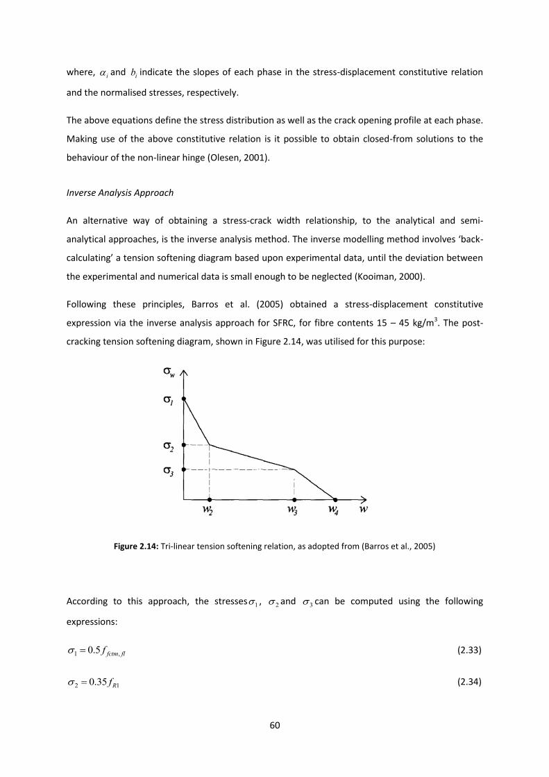
60
where, i and ib indicate the slopes of each phase in the stress-displacement constitutive relation
and the normalised stresses, respectively.
The above equations define the stress distribution as well as the crack opening profile at each phase.
Making use of the above constitutive relation is it possible to obtain closed-from solutions to the
behaviour of the non-linear hinge (Olesen, 2001).
Inverse Analysis Approach
An alternative way of obtaining a stress-crack width relationship, to the analytical and semi-
analytical approaches, is the inverse analysis method. The inverse modelling method involves ‘back-
calculating’ a tension softening diagram based upon experimental data, until the deviation between
the experimental and numerical data is small enough to be neglected (Kooiman, 2000).
Following these principles, Barros et al. (2005) obtained a stress-displacement constitutive
expression via the inverse analysis approach for SFRC, for fibre contents 15 – 45 kg/m3. The post-
cracking tension softening diagram, shown in Figure 2.14, was utilised for this purpose:
Figure 2.14: Tri-linear tension softening relation, as adopted from (Barros et al., 2005)
According to this approach, the stresses 1 , 2 and 3 can be computed using the following
expressions:
1 ,0.5 fctm flf (2.33)
2 10.35 Rf (2.34)
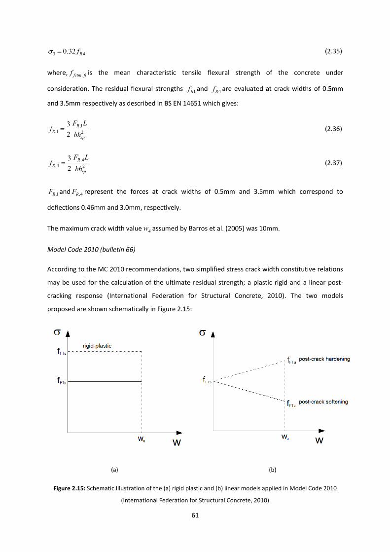
61
3 40.32 Rf (2.35)
where, ,fctm flf is the mean characteristic tensile flexural strength of the concrete under
consideration. The residual flexural strengths 1Rf and 4Rf are evaluated at crack widths of 0.5mm
and 3.5mm respectively as described in BS EN 14651 which gives:
,1
,1 2
3
2
R
R
sp
F Lf
bh (2.36)
,4
,4 2
3
2
R
R
sp
F Lf
bh (2.37)
,1RF and ,4RF represent the forces at crack widths of 0.5mm and 3.5mm which correspond to
deflections 0.46mm and 3.0mm, respectively.
The maximum crack width value 4w assumed by Barros et al. (2005) was 10mm.
Model Code 2010 (bulletin 66)
According to the MC 2010 recommendations, two simplified stress crack width constitutive relations
may be used for the calculation of the ultimate residual strength; a plastic rigid and a linear post-
cracking response (International Federation for Structural Concrete, 2010). The two models
proposed are shown schematically in Figure 2.15:
(a) (b)
Figure 2.15: Schematic Illustration of the (a) rigid plastic and (b) linear models applied in Model Code 2010
(International Federation for Structural Concrete, 2010)
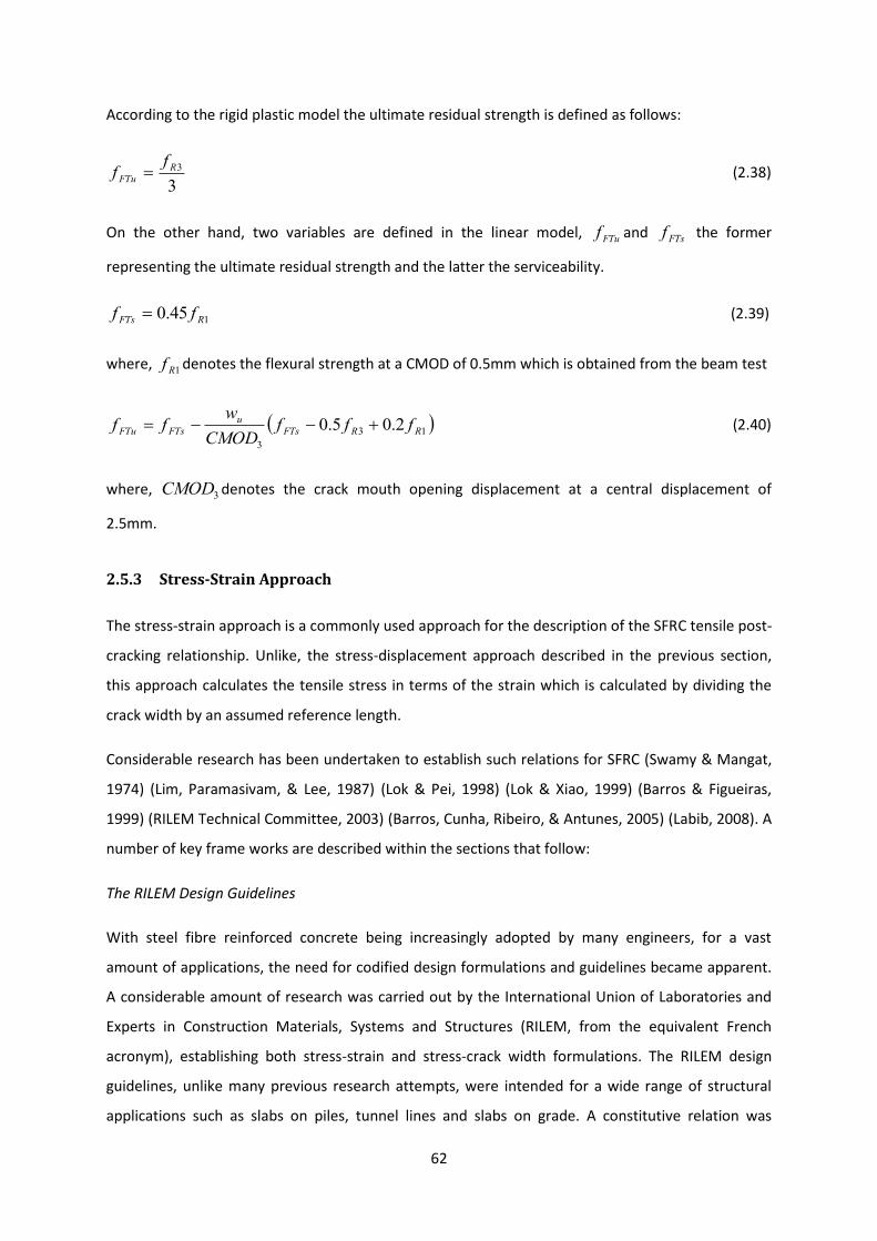
62
According to the rigid plastic model the ultimate residual strength is defined as follows:
3
3R
FTu
ff (2.38)
On the other hand, two variables are defined in the linear model, FTuf and FTsf the former
representing the ultimate residual strength and the latter the serviceability.
145.0 RFTs ff (2.39)
where, 1Rf denotes the flexural strength at a CMOD of 0.5mm which is obtained from the beam test
13
3
2.05.0 RRFTs
u
FTsFTu fffCMOD
wff (2.40)
where, 3CMOD denotes the crack mouth opening displacement at a central displacement of
2.5mm.
2.5.3 Stress-Strain Approach
The stress-strain approach is a commonly used approach for the description of the SFRC tensile post-
cracking relationship. Unlike, the stress-displacement approach described in the previous section,
this approach calculates the tensile stress in terms of the strain which is calculated by dividing the
crack width by an assumed reference length.
Considerable research has been undertaken to establish such relations for SFRC (Swamy & Mangat,
1974) (Lim, Paramasivam, & Lee, 1987) (Lok & Pei, 1998) (Lok & Xiao, 1999) (Barros & Figueiras,
1999) (RILEM Technical Committee, 2003) (Barros, Cunha, Ribeiro, & Antunes, 2005) (Labib, 2008). A
number of key frame works are described within the sections that follow:
The RILEM Design Guidelines
With steel fibre reinforced concrete being increasingly adopted by many engineers, for a vast
amount of applications, the need for codified design formulations and guidelines became apparent.
A considerable amount of research was carried out by the International Union of Laboratories and
Experts in Construction Materials, Systems and Structures (RILEM, from the equivalent French
acronym), establishing both stress-strain and stress-crack width formulations. The RILEM design
guidelines, unlike many previous research attempts, were intended for a wide range of structural
applications such as slabs on piles, tunnel lines and slabs on grade. A constitutive relation was

63
proposed to define the post-cracking tensile behaviour of SFRC using the residual flexural stress, as
obtained from three-point bending experiments. This relation is depicted in Figure 2.16.
Figure 2.16: Stress-strain relationship, as adapted from (RILEM, 2003)
The stresses illustrated in the above figure can be evaluated by making use of the following semi-
empirical relationships:
1 ,0.7 1.6fctm flf d (2.41)
2 ,10.45 R hf (2.42)
3 ,40.37 R hf (2.43)
where, ,fctm flf is the flexural characteristic tensile mean strength of the concrete, ,1Rf and ,4Rf are
the flexural residual stresses, corresponding to loads ,1RF and ,4RF at a crack mouth opening
displacement (CMOD) of 0.5mm (deflection of 0.46mm) and 3.5mm (deflection of 3.0mm)
respectively. In addition, size factor h can be evaluated from the following diagram:
c3.5 2.0
c
3
21 3
2
1
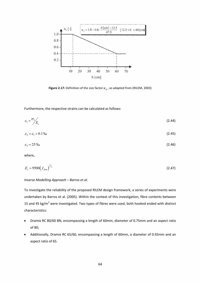
64
Figure 2.17: Definition of the size factor h , as adapted from (RILEM, 2003)
Furthermore, the respective strains can be calculated as follows:
11
cE
(2.44)
2 1 0.1‰ (2.45)
3 25‰ (2.46)
where,
1
39500c fcmE f (2.47)
Inverse Modelling Approach – Barros et al.
To investigate the reliability of the proposed RILEM design framework, a series of experiments were
undertaken by Barros et al. (2005). Within the context of this investigation, fibre contents between
15 and 45 kg/m3 were investigated. Two types of fibres were used, both hooked ended with distinct
characteristics:
Dramix RC 80/60 BN, encompassing a length of 60mm, diameter of 0.75mm and an aspect ratio
of 80;
Additionally, Dramix RC 65/60, encompassing a length of 60mm, a diameter of 0.92mm and an
aspect ratio of 65.
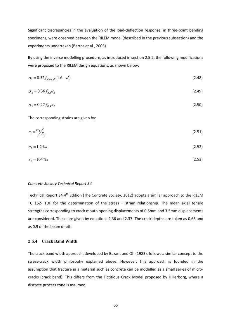
65
Significant discrepancies in the evaluation of the load-deflection response, in three-point bending
specimens, were observed between the RILEM model (described in the previous subsection) and the
experiments undertaken (Barros et al., 2005).
By using the inverse modelling procedure, as introduced in section 2.5.2, the following modifications
were proposed to the RILEM design equations, as shown below:
1 ,0.52 1.6fctm flf d (2.48)
2 ,10.36 R hf (2.49)
3 ,40.27 R hf (2.50)
The corresponding strains are given by:
11
cE
(2.51)
2 1.2‰ (2.52)
3 104‰ (2.53)
Concrete Society Technical Report 34
Technical Report 34 4th Edition (The Concrete Society, 2012) adopts a similar approach to the RILEM
TC 162- TDF for the determination of the stress – strain relationship. The mean axial tensile
strengths corresponding to crack mouth opening displacements of 0.5mm and 3.5mm displacements
are considered. These are given by equations 2.36 and 2.37. The crack depths are taken as 0.66 and
as 0.9 of the beam depth.
2.5.4 Crack Band Width
The crack band width approach, developed by Bazant and Oh (1983), follows a similar concept to the
stress-crack width philosophy explained above. However, this approach is founded in the
assumption that fracture in a material such as concrete can be modelled as a small series of micro-
cracks (crack band). This differs from the Fictitious Crack Model proposed by Hillerborg, where a
discrete process zone is assumed.

66
Figure 2.18: Crack band width approach developed by Bazant and Oh (1983), diagram adopted from (Kooiman,
2008)
Rather than using a direct stress-crack width relation, the width of the crack band is converted into a
strain. The outcome is a stress-strain relationship, which however uses similar fracture mechanics
concepts as the stress-crack width method. This method is commonly associated with the well-
known smeared-cracking approach in finite element analysis. In such an approach the formation of
many micro-cracks translate into a degradation of the stiffness at the integration point. (de Borst,
Remmers, Needleman, & Abellan, 2004). The application of the smeared cracking approach does not
require prior knowledge of the failure mode or the crack pattern that may arise in a pile-supported
slab. Such a method has the potential to be applied in the initial design stages in order to obtain a
better understanding of the mode of failure before a more detailed analysis and design takes place.
2.5.5 Critical Review of Constitutive Modelling Concepts
The inverse analysis approach presents itself as an easy to use method for the determination of the
structural properties. This approach can usually be accomplished using commercial packages.
Furthermore it would be applicable in the design of pile supported slabs as fewer parameters would
need to be verified. On the downside, such a method may not provide a full understanding of the
behaviour of the SFRC (Kooiman, 2000). Furthermore, the relation obtained can only be applied to
the structural situation at hand. Such a method does not allow the determination of a large number
of parameters with great accuracy.
Implementing the inverse analysis method using a stress-crack width response does not yield ‘an
unambigious stress-crack width relation’ as shown in Chapter 7 and discussed by (Kooiman, 2000).
The RILEM and Barros (2005) stress-strain models were described. Barros questioned the accuracy of
the RILEM stress-strain model. Technical Report 34 (2012 Draft) have adopted the stress-strain
approach proposed by RILEM. However, a few small adjustments were made in the constitutive
response that they implemented.
67
2.6 Concluding Remarks
The literature review highlighted the benefits and drawbacks of the beam and round determinate
plate (RDP) tests currently used to determine the flexural properties of SFRC. Although beam tests
allow for the derivation of the material properties they exhibit more scatter than RDP tests
(Lambrechts A. N.,2007). The RILEM beam test setup, as adopted by BS EN 14651, allows for the
direct measurement of the crack mouth opening displacement (CMOD) unlike conventional RDP
tests. This is its major advantage and the reason that it has been considered in the present work.
On the other hand, statically determinate RDP tests are more representative of the in situ behaviour
of SFRC slabs as the position of the cracks is not predetermined by a notch. The repeatability of the
crack pattern as well as the low scatter reported by previous researchers (Bernard & Pircher, 2000)
(Lambrechts A. N.,2007) are important benefits. The main drawback in such tests is the difficulty of
directly measuring crack widths using the recommended test setup. This is a significant disadvantage
since the residual flexural resistance of SFRC depends on the CMOD. Therefore, the standard RDP
test arrangement was modified in some of the author’s tests by loading the slabs from their
underside to allow a direct measurement of crack width. The resulting crack width measurements
were related to the applied loads and the displacements yielding some interesting results.
The constitutive modelling approaches for SFRC were reviewed forming a stepping stone to the
modelling approach selected in this work. The discrete crack Fictitious Crack Model framework
(Hillerborg, 1980) appears to be a realistic representation of the fracture mechanics that govern the
behaviour of SFRC. The main drawback of conventional discrete crack approaches is that the position
of the cracks needs to be known in advance of the analysis. The smeared crack approach is founded
on the assumption that concrete fracture occurs as a series of micro cracks. Although no prior
knowledge of the crack positions is required when using this approach, only limited crack width
information can be obtained. Using a discrete crack approach appears to be the most effective way
in obtaining crack width information from the NLFEA and is the principal procedure adopted in the
present study.The post cracking response of the SFRC is modelled indirectly in the current work
using assumed stress-crack opening relationship (-w) relationships which were derived by trial and
error using inverse analysis. The method involves the back-calculation of a -w relationship that is
systematically adjusted by trial and error to fit an experimentally determined load displacement
response. The alternative and much more complex modelling approach, which is not considered in
the present research, is to model individual fibres within the concrete matrix accounting for
slippage.
68
Chapter Three
Design of SFRC Pile Supported Slabs
3.1 Background
The increasing application of SFRC in commercial and industrial ventures has led to a demand for a
unified code of practice (The Concrete Society, 2007). Over the past few years a considerable
number of design recommendations have been proposed for the determination of material
properties and design of SFRC (British Standards Institution, 2005) (Destree, 2000) (Destree, 2005)
(International Federation for Structural Concrete, 2010) (Lambrechts A. N., 2003) (RILEM Technical
Committee, 2002) (The Concrete Society, 2003) (The Concrete Society, 2007) (The Concrete Society,
2012).
This chapter reviews the existing methods for the design and analysis of SFRC pile-supported slabs.
3.2 Design Aspects
3.2.1 General Overview
One of the most promising applications of Steel Fibre Reinforced Concrete (SFRC) is the construction
of pile supported slabs (The Concrete Society, 2007). The construction of slabs on piles usually
occurs when the ground is unable to adequately support the slab and its loads. This is particularly
applicable to industrial floors, where very high loads frequently arise in combination with poor
ground conditions. Key factors which determine the thickness of industrial pile-supported slabs
include the pile spacing and diameter as well as racking and wheel loads. All of the above are
discussed in the sections that follow:
3.2.2 Anatomy of a Pile Supported Slab
The past few decades have seen a huge increase in the use and design of pile supported slabs
incorporating only steel fibres (Destree, 2005). The typical pile spacing ‘ranges from 3m to 5m’ and
‘with a span to depth ratio of 15’ (The Concrete Society, 2003) (Destree, 2004). Typical thicknesses
range from 200mm to 320mm (The Concrete Society, 2007). The dosages normally used in pile
supported slabs range from 35 – 50 kg/m3 with 45 kg/m3 being a very common dosage (Hedebratt &

69
Silfwerbrand, 2004) (The Concrete Society, 2007). Omitting the traditional reinforcement can yield
numerous benefits; in terms of construction time, improved ductility and better corrosion resistance
(Silfwerbrand, 2008).
3.2.3 Design Loading
The majority of pile-supported slabs are designed for industrial and commercial purposes (The
Concrete Society, 2007). Such applications include the construction of large warehouse and factory
floors. TR 34 (The Concrete Society, 2003) makes reference to three types of loading; Uniformly
Distributed Loads (UDL), Line Load (LL) and Point Loads (PL).
UDLs include blocked pallet loads stacked one on top of the other, loads from fixed machinery and
equipment. According to the recommendations of TR34, the maximum height for such pallets is
limited to 4m. In many cases fixed machinery is supported on bases independent of the floor. The
effect of the vibration of the machinery should be taken into account in the dynamic loading of the
slab (The Concrete Society, 2003).
Point loads include heavy racking leg loads from racking pallets as well as wheel loads from heavy
good vehicles or forklift trucks. In some cases, the wheel loads due to heavy goods vehicle such as a
counterbalance truck can affect a particular area of the slab. As a result, large bending moments of
similar magnitude as the static loads can occur (The Concrete Society, 2012). In such cases the
effects of cyclic loading and fatigue need to be addressed accordingly. Heavy point loads can also
arise from the supports of mezzanines that are frequently constructed in industrial warehouses (The
Concrete Society, 2003). Typical point loads can vary between 35kN – 100kN.
Line loads can arise from dividing walls or other partitions (Bekaert, 2009) as well as ‘rail mounted
fixed equipment’ (The Concrete Society, 2003). Equipment mounted on rails can be considered as
line loads if the rails are mounted directly on the slab. However, if they are mounted on base plates
then they can to be designed as point loads.
3.2.4 Pathology of Pile – Supported Slabs
In the ultimate limit state two distinct modes of failure can occur; flexural failure and punching
shear. The most common type of flexural failure in reinforced concrete slabs is the so-called ‘folded-
plate mechanism’ (Kennedy & Goodchild, 2003). This type of mechanism consists of positive and
negative yield lines running parallel to each other (Figure 3.1). The second type of failure mechanism

70
that can occur is a conical collapse mechanism around the perimeter of the pile head. Punching
shear failures can also occur at the piles (Figure 3.4).
However, one of the biggest challenges is to achieve a satisfactory performance of SFRC pile
supported slabs at the serviceability limit state. In a number of cases, slabs have failed to satisfy the
serviceability limit state owing to severe cracking (Hulett, 2011). Although cracking may not result in
a catastrophic failure, it impairs the slab performance considerably. In addition the financial
repercussions should also be taken into account, especially considering the transport and/or
removal of heavy machinery, forklift trucks, racking pallets etc. The temporary halt of the operations
can be very costly.
3.3 Elastic Design
Elastic design methods have been used in the past for the design of pile supported slabs. In the
serviceability limit state it is possible to check whether cracking is likely to occur (The Concrete
Society, 2007). A number of design methods adopt elastic design principles such as the Dutch Code
NEN 6720 (The Concrete Society, 2007) and Bekaert (Thooft, 1999).
The Dutch Code NEN 6720 recommends that pile-supported floors should be designed elastically, at
the Ultimate Limit State (ULS). According to NEN 6720, the maximum design (support) moment that
a pile-supported slab has to be designed for is given by the following expression:
2M qL (3.1)
where, denotes the moment coefficient and is determined by the code, q denotes the applied
load and Ldenotes the span in consideration.
With regard to the above equation, a number of recommendations exist with regard to the
determination of the moment coefficient . The Dutch Code NEN 6720 recommends that:
0.132 is used for internal panels
0.178 is used when dealing with external panels
And 0.190 is used when corner panels are considered
The slab is divided into two edge strips, of width equivalent to 4L and one middle strip of
2L
. It
allows the determination of the ultimate design moment from elastic or finite element analysis as an
71
alternative to the above design method. Furthermore, beam tests are used to obtain the material
properties of the required SFRC.
The Dutch code uses mean rather than characteristic strengths. This mainly has to do with the load
re-distribution that occurs in such a structural element. It is argued that by using the characteristic
strengths for such elements one can obtain an overly conservative design solution.
In NEN 6720, only Uniformly Distributed Loads (UDL) are incorporated in the design procedure. Even
line loads arising from forklift trucks or racking loads are converted to an equivalent UDL. The sizing
of the slab in the Dutch code is done in such a way that no conventional reinforcement is required in
the tensile zone of the interior panels.
It can be argued that using an elastic method for the design of SFRC pile-supported slabs is
inefficient (The Concrete Society, 2007). This is due to the fact that the addition of steel fibres in the
dosages commonly used in pile supported slabs does not greatly increase the peak flexural
resistance of the concrete. The fibres come into effect after the peak flexural load by arresting crack
growth. The Dutch code allows for moment redistribution in the internal span of up to 20%.
3.4 Yield Line Method
The yield line theory, developed by Johansen (Johansen, 1972), is a widely accepted method for the
design of pile-supported slabs (The Concrete Society, 2007). The yield line theory is a plastic method
of design. It is an upper bound analysis requiring the postulation of a failure mechanism. Using the
principle of virtual work, by equating the external work done by loads and the internal work done by
the displacements, one can identify the failure load.
As described in section 3.2.4, SFRC pile-supported slabs give rise to two principal modes of failure
(Kennedy & Goodchild, 2003) (The Concrete Society, 2012).The first is widely known as the Folded
Plate Mechanism and is characteristic of flexural failure (Figures 3.1 and 3.2). The second is the
conical collapse mechanism. Technical Report 34 (The Concrete Society, 2012) provides some
guidance regarding the calculation of both mechanisms, applying Classical Yield Line Theory.

72
Figure 3.1: Schematic depiction of the wide beam failure mechanism in a pile-supported ground floor, as
adopted from (Kennedy and Goodchild, 2003)
(a) (b)
Figure 3.2: Folded Plate Failure Mechanism in (a) an exterior (perimeter) and (b) in an interior panel under
uniformly distributed load, adopted from (The Concrete Society, 2012)
Figure 3.2 illustrates the behaviour of the Folded Plate Failure Mechanism in the case of an exterior
and interior panel under a UDL. The ultimate collapse load is found by equating the external and
internal work.

73
In the case of an internal panel:
8
2
eu
np
LqMM (3.2)
where, pM denotes the sagging (positive) moment, nM denotes the hogging (negative) moment,
uq represents the UDL, and eL represents the effective span which TR34 defines as:
ce hLL 7.0 (3.3)
The ultimate collapse load of an exterior panel can be obtained from the following expression:
2
2
112 eu
p
np Lq
M
MM
(3.4)
The equation can be simplified further, assuming that np MM .
83.5
2
eu
np
LqMM (3.5)
The second load case, considered in the design of SFRC pile-supported slabs, is for concentrated line
loads. Such loads may arise from applications such as racking pallets and mezzanine supports.
(a) (b)
Figure 3.3: Folded Plate Failure Mechanism in (a) an exterior (perimeter) and (b) in an interior panel under
concentrated line load, adopted from (The Concrete Society, 2012)

74
The ultimate moment of resistance under a concentrated load in an interior panel is given by the
following equation (The Concrete Society, 2012):
84
2
e
sw
e
lnp
Lq
LQMM (3.6)
where, pM denotes the sagging (positive) moment, nM denotes the hogging (negative) moment,
lQ denotes the line load, uq represents the self weight of the pile supported slab, and eL represents
the effective length defined in equation 3.7:
ce hLL 7.0 (3.7)
In the case of the exterior (perimeter) panels, this equation becomes:
842
2
esweln
p
LqLQMM (3.8)
The equation can be simplified further, if np MM .
63
2
eswel
np
LqLQMM (3.9)
The second yield line pattern is one that involves a circular fan of radius, r at each pile (Figure 3.4).
Figure 3.4: Schematic depiction of the circular fan failure mechanism in a pile-supported ground floor, as
adapted from (Kennedy and Goodchild, 2003)
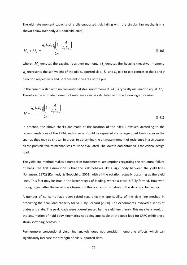
75
The ultimate moment capacity of a pile-supported slab failing with the circular fan mechanism is
shown below (Kennedy & Goodchild, 2003):
2
13
21
21
LL
ALLq
MM
u
np (3.10)
where, pM denotes the sagging (positive) moment, nM denotes the hogging (negative) moment,
uq represents the self weight of the pile supported slab, 1L and 2L pile to pile centres in the x and y
direction respectively and A represents the area of the pile.
In the case of a slab with no conventional steel reinforcement pM is typically assumed to equal nM
Therefore the ultimate moment of resistance can be calculated with the following expression:
2
13
21
21
LL
ALLq
M
u
(3.11)
In practice, the above checks are made at the location of the piles. However, according to the
recommendations of the TR34, such checks should be repeated if any large point loads occur in the
span as they may be critical. In order, to determine the ultimate moment of resistance in a structure,
all the possible failure mechanisms must be evaluated. The lowest load obtained is the critical design
load.
The yield line method makes a number of fundamental assumptions regarding the structural failure
of slabs. The first assumption is that the slab behaves like a rigid body between the yield lines
(Johansen, 1972) (Kennedy & Goodchild, 2003) with all the rotation actually occurring at the yield
lines. This fact may be true in the latter stages of loading, where a crack is fully formed. However,
during or just after the initial crack formation this is an approximation to the structural behaviour.
A number of concerns have been raised regarding the applicability of the yield line method in
predicting the peak load capacity for SFRC by Bernard (2000). The experiments involved a series of
plates and slabs. The peak loads were overestimated by the yield line theory. This may be a result of
the assumption of rigid body kinematics not being applicable at the peak load for SFRC exhibiting a
strain softening behaviour.
Furthermore conventional yield line analysis does not consider membrane effects which can
significantly increase the strength of pile supported slabs.
76
3.5 Punching Shear
Considerable research has been carried out to determine the effect of fibres on the punching shear
capacity of slabs (Patel, 1970) (Criswell, 1974) (Swamy & Ali, 1982) (Alexander & Simmonds, 1992)
(Labib, 2008). However, the majority of research has dealt with the incorporation of the fibres as an
addition to traditional steel reinforcement. Previous research has shown that steel fibres increase
the punching shear resistance of slabs (Criswell, 1974) (Alexander & Simmonds, 1992).
In 1970, Patel (Patel, 1970) investigated the effect of adding fibres into seven slab column
connections with conventional reinforcement. The steel fibre dosages used were 0.574% and 1.2%
by volume. The incorporation of the fibres was observed to enhance the load required for visible
flexural cracking of the slab. Although the cracking pattern remained the same, increasing the fibre
dosage from 0.574% to 1.2% resulted in the cracks becoming smaller. It was noted that as the
dominant mode of failure was flexural the fibres were effective in preventing punching shear.
The experimental work of Criswell (1974), on the addition of fibres in square column stubs with
traditional reinforcement, confirmed the positive effect of fibres in preventing punching shear
failure. Four stubs in total were tested, two with a reinforcement ratio of 1.0% and two with a
reinforcement ratio of 1.88%. All the slabs were reinforced with a dosage of 1.0% of steel fibres by
volume. The behaviour of the slabs with a reinforcement ratio of 1.0% was governed by flexural
failure whereas the behaviour of the slabs with a reinforcement ratio of 1.88% was governed by
punching shear. It was noted that the incorporation of the fibres increased the residual strength
even if the failure was due to punching. In addition, the highest percentage increase in failure
strength was provided by the fibres added in the slab reinforced with 1.0%.
Swamy and Ali (1982) also observed an increase in punching resistance from the addition of steel
fibres into 19 slabs with traditional reinforcement. The fibre content used varied from 0 to
94.2kg/m3. Alexander et al (1992) tested six square slabs of dimensions 2750mm x 2750mm x
155mm. The fibre amounts used varied from 0 to 69 kg/m3. An increase in the punching shear
resistance of slabs in the region of 20% - 30% was noted. The above findings were confirmed by the
experimental research of Tan and Paramasivam (1994).
The experimental work undertaken by Labib (2008) on circular SFRC slabs concluded that increasing
the fibre content has a positive effect on the ultimate failure load. Higher fibre dosages resulted in
smaller deflections at the same loading levels, thus confirming the findings of Swamy and Ali (1982).
In 2011 Susetyo et al., tested 10 panels under shear investigating the addition of steel fibres into
slabs with traditional reinforcement. The panels incorporated fibre contents from 0.5% - 1.5% by
77
volume. Their results demonstrated that the slabs with increasing fibre content exhibited smaller
crack widths as well as an enhanced shear resistance between 22% and 130%.
The punching shear response of pile-supported slab can significantly be affected by the inclusion of
fibres. The inclusion of the fibres, apart from increasing the failure load (Swamy & Ali, 1982)
(Alexander & Simmonds, 1992) (Tan & Paramasivam, 1994) (Labib, 2008) (Susetyo et al., 2011) can
also increase the ductility (Swamy & Ali, 1982) (Labib, 2008) (Susetyo et al., 2011) of the slab. The
crack width at a pre-specified load is reduced, as fibres help bridge cracks (Labib, 2008). Fibres can
act as shear reinforcement by transferring tension across the cracks. In addition, the depth of the
flexural compression zone may increase thus increasing the shear resistance.
The punching shear capacity of a structural element can be calculated by checking the shear at a pre-
determined distance away from the pile-head. BS 8110, Eurocode 2 as well as the NEN 6720, adopt
this logic. However, the critical distance d varies between codes.
NEN 6720 checks punching shear along a perimeter at a distance d from the pile face; whereas BS
8110 and EC2 check it at 1.5d and 2d, respectively, where d is the depth to the centre-line of the
tension reinforcement bars. However, all the fore-mentioned codes make the assumption that
conventional steel reinforcement is incorporated in the design.
The shear resistance of SFRC is taken as the sum of the resistances provided by the concrete and
fibres. TR34 takes the shear resistance provided by the concrete in SFRC only slabs as the minimum
shear resistance recommended by EC2 for members with conventional reinforcement which is given
by:
2123
1min, 035.0 ckc fkv (3.12)
In which the coefficient 1k is defined as follows:
12001 2k
d (3.13)
Consequently, the punching resistance of SFRC slabs without conventional flexural and shear
reinforcement is given by:
udvvV fc min, (3.14)
where, fv denotes the contribution of steel fibres in the punching shear capacity, d denotes the
effective depth and u denotes the control perimeter.

78
In the case where bars are not present, TR34 defines d as 0.75h. Technical Report 34 3rd edition (The
Concrete Society, 2003) calculates the contribution of steel fibres to shear resistance fv in
accordance with the RILEM (2002) recommendations as follows:
,3 ,0.12f e ctk flv R f (3.15)
where, ,3eR and ,ctk flf denote the flexural strength ratio and the flexural strengths.
A minimum shear capacity of 3 2 1 210.035 ckk f is recommended by EC2 in the case of plain concrete.
Therefore the shear capacity in a slab with fibre-only reinforcement can be calculated by the
following expression (The Concrete Society, 2003):
3 2 1 21 ,3 ,0.035 0.12p c e ctk flP k f R f u d (3.16)
where, d denotes the effective depth of the section and u denotes the length of the perimeter at a
distance of 2d from the loaded area (Figure 3.5).
The above design method is also recommended by Technical Report 63 (The Concrete Society, 2007)
for SFRC slabs on piles without conventional reinforcement.
Technical Report 34 (2012 Final Draft) is of the view that the RILEM design guidelines overestimate
the increase in shear resistance provided by fibres. ‘In the absence of verifiable research’, it applies a
reduction of 50% to the contribution of the steel fibres assumed by RILEM. Consequently, TR34
(2012 Final Draft) takes the contribution of the fibres to shear resistance as:
4321015.0 rrrr ffff (3.17)
where, 1rf ’ 2rf ’ 3rf and 4rf are residual strengths at 0.5mm, 1.5mm, 2.5mm and 3.5mm
respectively.
Technical Report 34 (The Concrete Society, 2012)recommends that the punching shear failure should
be checked at both at the pile location, as well as, any other location where high point loads are
located. Should the punching shear stresses be critical, then increasing the slab depth is suggested as
the most appropriate design option.
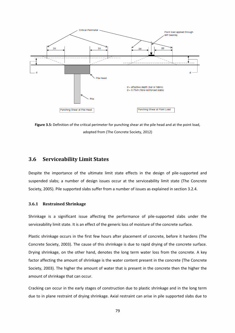
79
Figure 3.5: Definition of the critical perimeter for punching shear at the pile head and at the point load,
adopted from (The Concrete Society, 2012)
3.6 Serviceability Limit States
Despite the importance of the ultimate limit state effects in the design of pile-supported and
suspended slabs; a number of design issues occur at the serviceability limit state (The Concrete
Society, 2005). Pile supported slabs suffer from a number of issues as explained in section 3.2.4.
3.6.1 Restrained Shrinkage
Shrinkage is a significant issue affecting the performance of pile-supported slabs under the
serviceability limit state. It is an effect of the generic loss of moisture of the concrete surface.
Plastic shrinkage occurs in the first few hours after placement of concrete, before it hardens (The
Concrete Society, 2003). The cause of this shrinkage is due to rapid drying of the concrete surface.
Drying shrinkage, on the other hand, denotes the long term water loss from the concrete. A key
factor affecting the amount of shrinkage is the water content present in the concrete (The Concrete
Society, 2003). The higher the amount of water that is present in the concrete then the higher the
amount of shrinkage that can occur.
Cracking can occur in the early stages of construction due to plastic shrinkage and in the long term
due to in plane restraint of drying shrinkage. Axial restraint can arise in pile supported slabs due to
80
horizontal forces that develop between the underlying soil, the pile and the slab (Destree, 2000)
(Knapton, 2003). Shrinkage causes axial shortening of the slab. As a result tension forces arise, which
can cause cracking in axially restrained slabs. The uneven settlement of piles can also induce vertical
restraint forces thus affecting the load distribution in the slab (Thooft, 1999).
Technical Report 63 (The Concrete Society, 2007) proposed two different ways of controlling
shrinkage in pile-supported slabs. The first is by appropriate material specification (concrete mix,
specification of aggregates, etc.). The second involves the use of a membrane to reduce the friction
between the soil and the slab. It is also recommended to use joints and conventional reinforcement
as a tool for minimising the shrinkage induced cracking. The pile support shall not be built into the
slab. Doing so will induce additional restraint stresses. However, the pile bearing should be designed
so that ‘it provides full support over the contact area’ (The Concrete Society, 2012).
The problem of cracking due to restrained shrinkage is not well understood partially as a result of
the difficulties in accurately measuring in plane stresses induced by shrinkage. Technical Report 63
(The Concrete Society, 2007) proposed the following expression for calculating the shrinkage
stresses in slabs with full restraint. This expression would be relevant to pile-supported slabs due to
the additional restraint offered by the piled supports. However, it is only a rule of thumb and should
be used with some caution:
1
cm shsh
Ef
(3.18)
where, sh is the shrinkage strain and is the creep coefficient.
The approach taken in Technical Report 34 (2012 Final Draft) is to deal with shrinkage issues at a
material level. This can be achieved by selecting appropriate concrete mixes with low water content
as well as selecting suitable water-reducing and shrinkage reducing admixtures.
3.6.2 Cracking
A major origin of cracking, as explained in section 3.6.1 is caused by the axial shortening due to
shrinkage coupled with the horizontal forces developing between the ground, the pile head and the
slab. The presence of severe cracking can impair the serviceability performance of a pile supported
slab. Severe cracking can affect the floor flatness. Severe cracking could lead to damage of the
concrete due to traffic over the crack. As a result spalling can occur at cracks (Fricks, 1992).

81
There are aesthetic objections regarding the amount of cracking (Fricks, 1992) but these are limited
in the cases where pile-supported slabs are used for commercial ventures such as large shopping
malls. However, cracking is also a problem in industrial floors. The crack width calculations in design
standards and the RILEM design guidelines are only applicable to structures incorporating
conventional reinforcement in strain softening materials. This is due to the fact that it is difficult to
quantify the effect of the fibres on crack widths.
3.6.3 Deflection
Technical Report 34 (The Concrete Society, 2012) claims that any slabs designed using their
recommendations (outlined in the previous subsections) should have much lower deflections than
the EC2 limits of the span/250. In effect the deflections obtained will be significantly smaller than in
suspended flat slabs which are considerably more slender. As a result, deflection checks are not
deemed necessary for steel fibre reinforced pile supported slabs (The Concrete Society, 2012).
3.7 Shortcomings of Current Design Guidelines
Having reviewed, the different code provisions as well as the design approaches for the analysis and
design of SFRC pile-supported slabs, the need for a unified design approach has become apparent.
At the time of writing, EC2 gives no guidance on the design of SFRC. A few design codes, such as the
Dutch Code NEN 6720 provide some guidance regarding the design of pile-supported slabs.
However, the Dutch guidelines are limited to the cases where conventional reinforcement is
provided in addition to fibres.
Elastic Design
Elastic design guidelines have been in use in the past for the analysis and design of pile-supported
slabs (Thooft, 1999) (The Concrete Society, 2003) (Bekaert, 2009) (The Concrete Society, 2007).
Although such design methods have been used successfully in structures encompassing traditional
reinforcement, their effectiveness in design a SFRC section can be questioned as they fail to
recognise the beneficial effect of the ductility introduced by the fibres. In pile-supported slabs fibre
dosages are usually insufficient to significantly increase the flexural strength above that of plain
concrete (The Concrete Society, 2007). In fact, the addition of the fibres is to control the crack
widths at the serviceability limit state. Using elastic guidelines for the design of pile-supported slabs
may produce an over-conservative design section (as the effect of the fibres is not taken into
account).
82
Yield Line Method
The yield line method constitutes a theoretical upper bound design method for the design of pile-
supported slabs. Using the principle of virtual work, the ultimate failure load is found by equating
the external and internal work. A drawback of using this method is that it does not give any
information on the performance of the slab at the serviceability limit state.
The yield line method makes a number of assumptions which are only approximate, particularly for
materials exhibiting a ‘tension softening’ response. The first assumption is that the slab behaves like
a rigid body between yield lines (Johansen, 1972) (Kennedy & Goodchild, 2003). All the curvature is
assumed to be concentrated in the yield lines which occur at the cracks. In practice, ‘quasi-elastic
deformations can occur due to possible flexural, membrane, shear flexural and torsional stresses’
(Bernard et al., 2001). The regions of the slab between yield lines, behave as a rigid body at
sufficiently large crack widths as the elastic deformations of the slab are small in comparison to the
total deflection of the slab. However, this is not the case in the early stages of loading when cracks
first form.
The moment along the yield line is also assumed to be constant (Johansen, 1972) (Kennedy &
Goodchild, 2003). This assumption is considered reasonable for materials with a strain hardening
response such as concrete with traditional steel reinforcement but may not be reasonable near the
peak load for materials exhibiting a strain softening response.
Punching Shear
Previous research has demonstrated the benefits of fibres in increasing punching shear resistance
(Swamy & Ali, 1982) (Alexander & Simmonds, 1992) (Tan & Paramasivam, 1994) (Susetyo et al.,
2011). However, the above research is somewhat limited to particular load cases, slab geometry and
fibre type (Labib, 2008). The majority of tests have also been carried out on slabs with conventional
reinforcement as well as steel fibres.
The RILEM (2002) recommendations were the first to take account of the positive effect of the fibres
in punching shear that could be applied to structures encompassing steel fibres in addition to
traditional reinforcement. As the RILEM recommendations are ‘not supported by published
research’ (The Concrete Society, 2012), Technical Report 34 (2012 Final Draft) propose a reduction of
50% on the proposed value.
Eurocode 2 gives guidance on punching shear in slabs with conventional reinforcement. No
recommendation is given for steel fibre only structures or even for the positive effects of the fibres
83
in addition to the existing reinforcement. Concrete Society Technical Report 63 (The Concrete
Society, 2007) claims that equation 3.13, which is based on the RILEM guidelines RILEM (2003), will
yield over conservative results according to experimental research.
Serviceability Limit States
There is a lack of authoritative design guidance regarding the serviceability limit state of SFRC slabs.
TR34 (4th Edition) suggests that most of the practical problems regarding crack widths and shrinkage
can be minimised at a material level by the appropriate selection of admixtures and cement.
Available guidance on the calculation of crack width, such as the RILEM guidelines, applies to
structural members that are reinforced with conventional reinforcement as well as fibres. None of
the codes deal with the calculation of crack widths in SFRC only slabs.
3.8 Concluding Remarks
The present survey of the state of the art has demonstrated that additional guidelines are required
for the design of SFRC pile-supported slabs encompassing little or no reinforcement. There are
sufficient gaps and ‘grey’ areas in the current knowledge. At the time of writing, EC2 gives no
guidance on the design of structural elements reinforced with SFRC. The Dutch Code NEN 6720 limits
its guidance to the case where conventional reinforcement is provided in addition to fibres.
Although elastic analysis has been used for the design of pile-supported slabs (The Concrete Society,
2007) such an approach does not take into account the benefits of steel fibres on the post-cracking
response of SFRC. As a result an over-conservative design can be produced. Yield line analysis is
commonly used for the design of SFRC slabs at the design ultimate limit state. It makes a number of
simplifying assumptions. For example, the moment is assumed to be constant along yield lines and
the slab is assumed to behave as a rigid body between the yield lines. Further research is required to
investigate the applicability of these assumptions to SFRC slabs without traditional reinforcement.
The subsequent chapters in the present work examine the ability of the yield line method to predict
the response of SFRC slabs without conventional reinforcement. Emphasis is placed on determining
the variation of the moment along the yield lines in both RDP and pile supported slabs.
Punching shear in SFRC structures encompassing traditional reinforcement has been dealt in the
past by a number of researchers (Patel, 1970) (Criswell, 1974) (Swamy & Ali, 1982) (Alexander &
Simmonds, 1992) (Tan & Paramasivam, 1994) (Susetyo et al., 2011) (Maya Duque et al., 2012).
Unfortunately the above research is limited to particular load cases and fibre types (Labib, 2008).

84
RILEM (2002) was the first to provide some guidelines taking into account the effect of fibres in
increasing punching shear resistance. However, these guidelines are confined to cases where
traditional steel reinforcement is present. EC2 on the other hand, makes no provisions for the effect
of steel fibres on the shear capacity. This highlights the need for the present work to evaluate
empirically the increase in punching shear offered by the addition of steel fibres to slabs without
conventional reinforcement. The control of crack widths at the serviceability limit is of fundamental
importance to the design of SFRC pile and ground supported slabs. The available design guidance on
the calculation of the crack widths only applies to structures with traditional steel reinforcement.
The determination of crack widths is therefore investigated in the present work by relating
experimentally determined crack widths to imposed displacements using yield line analysis and
NLFEA. The next chapter describes the experimental methodology adopted in the current research
including the procedures used to measure crack widths in the RDP and continuous slab tests.
85
Chapter Four
Experimental Programme
4.1 Introduction
The Literature Review gives an overview of the behaviour, and methods used for the analysis and
design of pile-supported slabs. The lack of a universally accepted method for the design of such slabs
is evident.
The present chapter describes the experimental programme which was undertaken to develop a
better understanding of the behaviour of SFRC slabs. The experimental results are subsequently
used to refine the NLFEA procedures described in Chapter Six. The aim of the present chapter is to
acquaint the reader with the experimental methodology that was followed within this research
project. Details of the SFRC mix design are given along with a description of the setup of each test.
Accordingly, a detailed description of the adopted instrumentation is presented herein.
4.2 Summary of Tests
Notched beams and round determinate plates (RDP) were tested in order to compare the material
properties given by each test. The resulting material properties were then used to predict the
measured responses of a series of indeterminate slabs. The tests also examined the relationship
between crack width and displacement in round plates and continuous slab tests. The ultimate aim
of the test programme was to gain an improved understanding of the behaviour of SFRC in pile –
supported slabs.
The present experimental programme consisted of four distinct stages; each stage was done in a
separate casting:
Cast 1 consisted of:
6 notched beam tests of 150mm x 150mm x 550mm which were tested in accordance with the
requirements of EN 14651 (British Standards Institution, 2005).
3 simply supported statically determinate round panels of diameter 1m and thickness of 125mm,
with three supports, tested as per the recommendations of the ASTM C1550: Standard Method

86
for Flexural Toughness of Fiber Reinforced Concrete. The slab depth was chosen to be the same
as the depth of the notched beam tests in order to minimise size effects.
Cast 2 consisted of:
6 notched beam tests of 150mm x 150mm x 550mm which were tested in accordance with the
requirements of EN 14651 (British Standards Institution, 2005).
3 simply supported statically indeterminate round panels of diameter 1m and thickness of
125mm, with six supports, tested as per the recommendations of the ASTM C1550: Standard
Method for Flexural Toughness of Fiber Reinforced Concrete.
Cast 3 consisted of:
6 notched beam tests of 150mm x 150mm x 550mm which were tested in accordance with the
requirements of EN 14651 (British Standards Institution, 2005).
3 round panels of diameter 1m and depth of 125mm. Unlike the previous tests undertaken,
these would be tested with the load at the underside of the slab and the supports at the top.
This was done so that the cracking pattern, which in these tests occurs primarily at the
underside, forms on the topside so that it can be observed in more detail.
6 beam tests of dimensions 100mm x 100mm x 500mm, which were tested for flexural strength.
The influence of fibres was investigated by testing three beams with fibres and three without.
Cast 4 consisted of:
6 notched beam tests of 150mm x 150mm x 550mm which were tested in accordance with the
requirements of EN 14651 (British Standards Institution, 2005).
3 two span one-way slabs of length 3m, depth of 125mm and width of 500mm.
As in Cast 3, 6 beam tests of dimensions 100mm x 100mm x 500mm were tested for flexural
strength. Three of these beams were reinforced with fibres and three were made from plain
concrete.
More details of the experimental procedure as well as the casting are given within the sections that
follow:

87
4.3 Fabrication of Test Specimens
4.3.1 Concrete Mix Design
The concrete mix was designed to have a 28-day cube strength of 50MPa, with a medium workability
(slump 70mm – 100mm). The dosage of steel fibres used was 45 kg/m3, which represents 0.5% by
volume.
The concrete mix design that was chosen for the present study is presented in the table below:
Component Dosage (kg/m3)
Cement CEM I 52.5 R 350
Coarse Aggregate 1050
Fine aggregate 900
Superplasticizer 2.25
Steel Fibres 45
Water 130
Table 4.1: Concrete mix design adopted for the current study
Ordinary Portland cement 52.5R was used in order to get the targeted 28-day compressive cube
strength of 50 MPa. All the cement used was from a single batch, which was acquired shortly before
the commencement of the experimental programme.
Coarse aggregate with a maximum size of 10mm, rather than the industry standard of 20mm, was
used in order to improve the interaction between the steel fibres and the concrete. Sand with a
maximum particle size of 5mm was used for the fine aggregate. ConPlast SP430 superplasticizer was
used to increase the workability of the concrete. It is chloride free with low alkali content (FOSROC,
2007).
Low carbon cold-drawn Wirand hooked-end fibres, with reference FF3, were added to the mix at a
dosage of 45 kg/m3. This dosage is representative of that typically used in pile-supported slab
construction (The Concrete Society, 2007). The fibres have a length of 50mm, a diameter of 0.75mm
and an aspect ratio of 67. The Re3 value corresponding to this type of fibre at the present dosage is
108% according to the manufacturer’s technical data sheet (Maccafferi). These were loose type
fibres, which were added to the mix by hand.
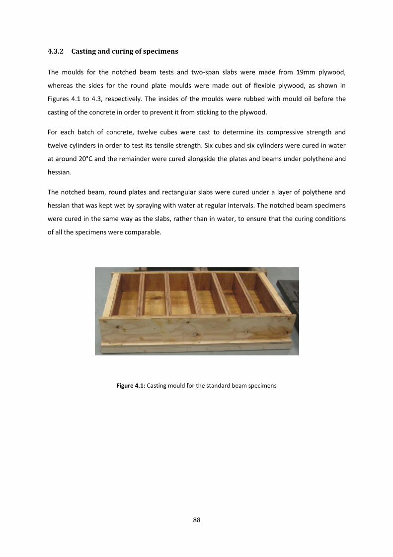
88
4.3.2 Casting and curing of specimens
The moulds for the notched beam tests and two-span slabs were made from 19mm plywood,
whereas the sides for the round plate moulds were made out of flexible plywood, as shown in
Figures 4.1 to 4.3, respectively. The insides of the moulds were rubbed with mould oil before the
casting of the concrete in order to prevent it from sticking to the plywood.
For each batch of concrete, twelve cubes were cast to determine its compressive strength and
twelve cylinders in order to test its tensile strength. Six cubes and six cylinders were cured in water
at around 20°C and the remainder were cured alongside the plates and beams under polythene and
hessian.
The notched beam, round plates and rectangular slabs were cured under a layer of polythene and
hessian that was kept wet by spraying with water at regular intervals. The notched beam specimens
were cured in the same way as the slabs, rather than in water, to ensure that the curing conditions
of all the specimens were comparable.
Figure 4.1: Casting mould for the standard beam specimens

89
Figure 4.2: Casting mould for the round panel specimens
Figure 4.3: Casting mould for the long beam tests
4.4 Beam Tests
4.4.1 Geometry of Test Specimens
The material properties of the SFRC were determined by testing notched beams with the geometry
shown in Figure 4.4. The test procedure described within this subsection is taken from the
recommendations of BS EN 14651 (British Standards Institution, 2005) which is based on the RILEM
162-TDF Beam Bending Test (RILEM Technical Committee, 2000).

90
Figure 4.4: Three-point bending beam test adopted for the present study, as per the recommendations of BS
EN 14651
The test specimens were notched using wet sawing, as described in BS EN 14651. The notch was
made at 90° from the trowled face of the beam. The width of the notch for each beam was less than
5mm and the height was 25mm ± 1mm from the tip of the notch.
4.4.2 Instrumentation
For the present study, the crack mouth opening displacement (CMOD) is of particular interest. To
measure the CMOD, a displacement transducer was mounted on the underside of the beam along its
longitudinal centre-line. The vertical distance y (Figure 4.5) was 4mm, as dictated by BS EN 14651.
The CMOD was also calculated from the beam displacement following the recommendations of BS
EN 14651.
The vertical displacement was measured with a pair of transducers mounted on each side of the
beam. The transducers were attached to a rigid frame that was supported on the top of the beam
over its supports as shown in Figures 4.6 and 4.7. This was done in order to measure the ‘true’
vertical deflection and not the sum of the deflection and the bedding in at the supports. As above,
this was done in accordance with BS EN 14651. The beam was simply supported on two steel rollers,
as shown in Figure 4.6, which only provided vertical restraint.
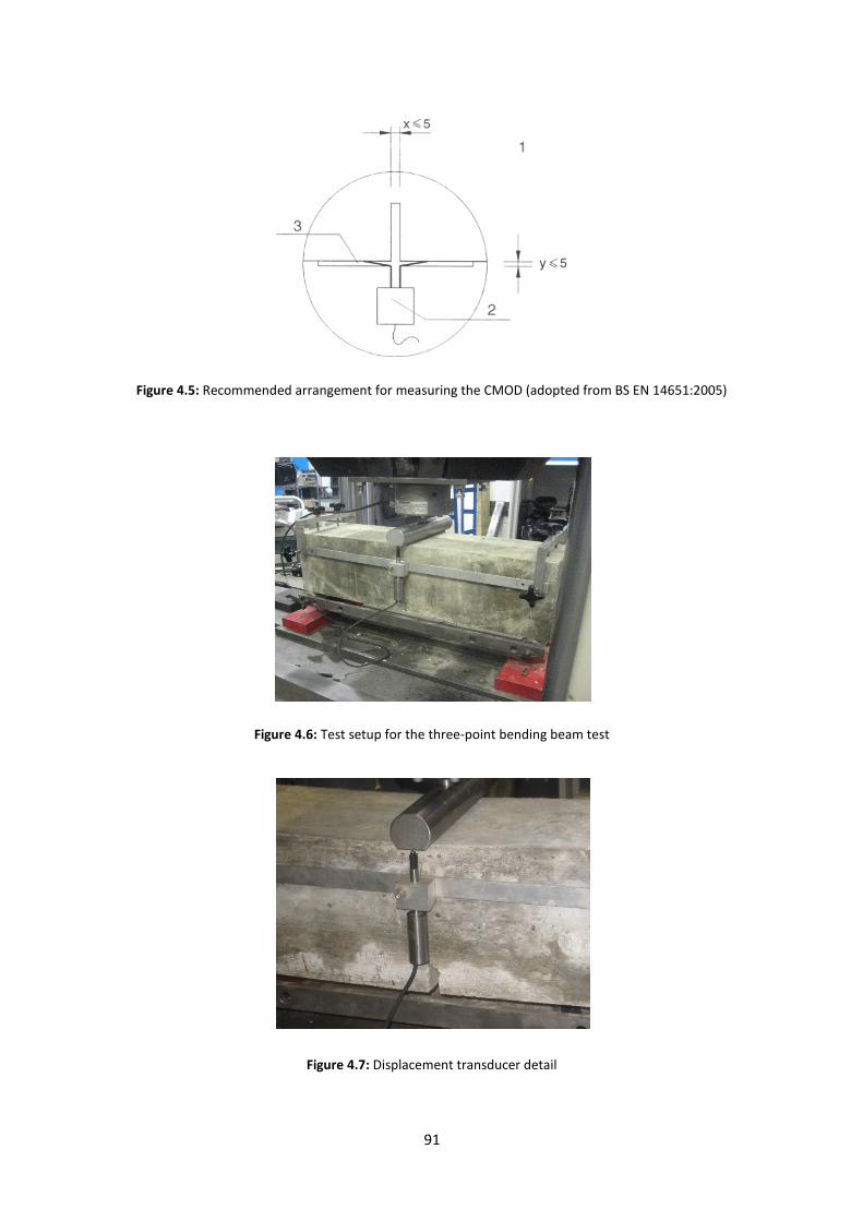
91
Figure 4.5: Recommended arrangement for measuring the CMOD (adopted from BS EN 14651:2005)
Figure 4.6: Test setup for the three-point bending beam test
Figure 4.7: Displacement transducer detail
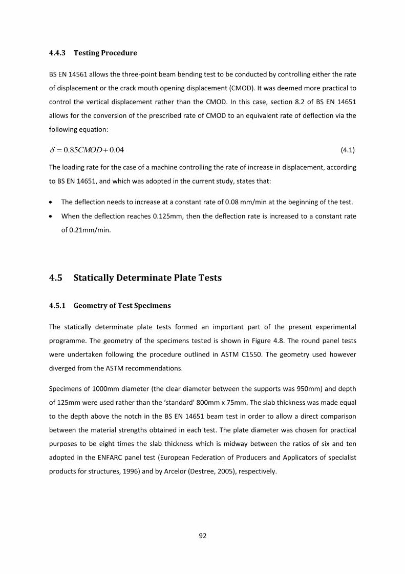
92
4.4.3 Testing Procedure
BS EN 14561 allows the three-point beam bending test to be conducted by controlling either the rate
of displacement or the crack mouth opening displacement (CMOD). It was deemed more practical to
control the vertical displacement rather than the CMOD. In this case, section 8.2 of BS EN 14651
allows for the conversion of the prescribed rate of CMOD to an equivalent rate of deflection via the
following equation:
04.085.0 CMOD (4.1)
The loading rate for the case of a machine controlling the rate of increase in displacement, according
to BS EN 14651, and which was adopted in the current study, states that:
The deflection needs to increase at a constant rate of 0.08 mm/min at the beginning of the test.
When the deflection reaches 0.125mm, then the deflection rate is increased to a constant rate
of 0.21mm/min.
4.5 Statically Determinate Plate Tests
4.5.1 Geometry of Test Specimens
The statically determinate plate tests formed an important part of the present experimental
programme. The geometry of the specimens tested is shown in Figure 4.8. The round panel tests
were undertaken following the procedure outlined in ASTM C1550. The geometry used however
diverged from the ASTM recommendations.
Specimens of 1000mm diameter (the clear diameter between the supports was 950mm) and depth
of 125mm were used rather than the ‘standard’ 800mm x 75mm. The slab thickness was made equal
to the depth above the notch in the BS EN 14651 beam test in order to allow a direct comparison
between the material strengths obtained in each test. The plate diameter was chosen for practical
purposes to be eight times the slab thickness which is midway between the ratios of six and ten
adopted in the ENFARC panel test (European Federation of Producers and Applicators of specialist
products for structures, 1996) and by Arcelor (Destree, 2005), respectively.
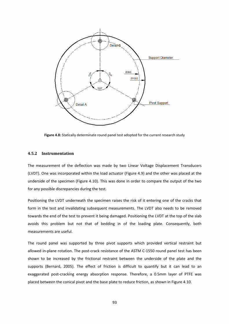
93
Figure 4.8: Statically determinate round panel test adopted for the current research study
4.5.2 Instrumentation
The measurement of the deflection was made by two Linear Voltage Displacement Transducers
(LVDT). One was incorporated within the load actuator (Figure 4.9) and the other was placed at the
underside of the specimen (Figure 4.10). This was done in order to compare the output of the two
for any possible discrepancies during the test.
Positioning the LVDT underneath the specimen raises the risk of it entering one of the cracks that
form in the test and invalidating subsequent measurements. The LVDT also needs to be removed
towards the end of the test to prevent it being damaged. Positioning the LVDT at the top of the slab
avoids this problem but not that of bedding in of the loading plate. Consequently, both
measurements are useful.
The round panel was supported by three pivot supports which provided vertical restraint but
allowed in-plane rotation. The post-crack resistance of the ASTM C-1550 round panel test has been
shown to be increased by the frictional restraint between the underside of the plate and the
supports (Bernard, 2005). The effect of friction is difficult to quantify but it can lead to an
exaggerated post-cracking energy absorption response. Therefore, a 0.5mm layer of PTFE was
placed between the conical pivot and the base plate to reduce friction, as shown in Figure 4.10.
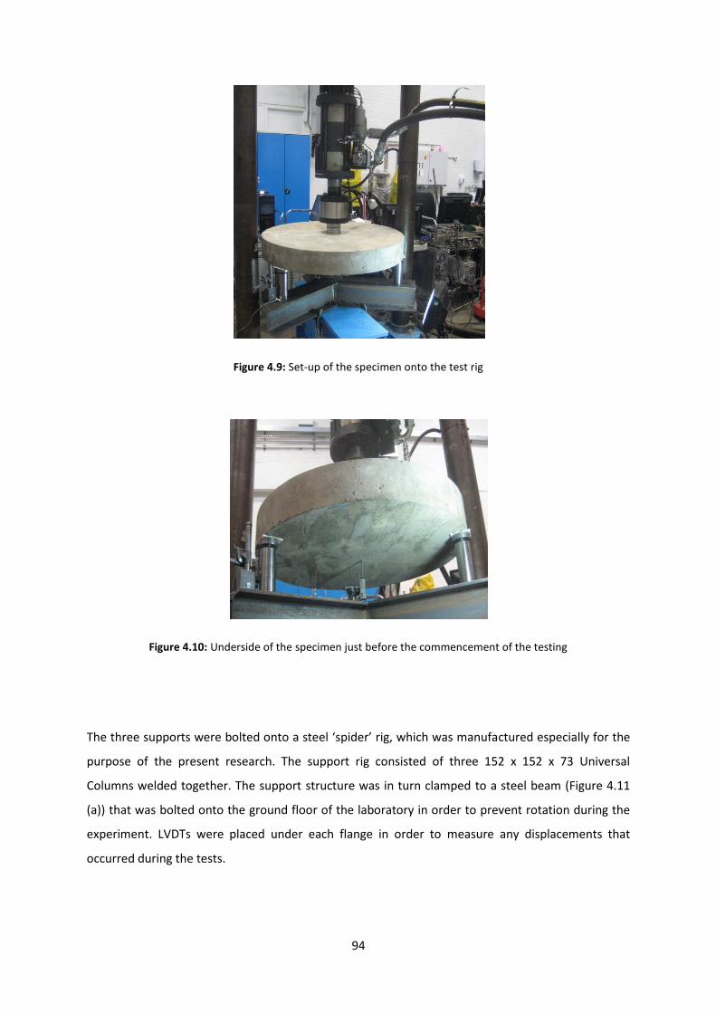
94
Figure 4.9: Set-up of the specimen onto the test rig
Figure 4.10: Underside of the specimen just before the commencement of the testing
The three supports were bolted onto a steel ‘spider’ rig, which was manufactured especially for the
purpose of the present research. The support rig consisted of three 152 x 152 x 73 Universal
Columns welded together. The support structure was in turn clamped to a steel beam (Figure 4.11
(a)) that was bolted onto the ground floor of the laboratory in order to prevent rotation during the
experiment. LVDTs were placed under each flange in order to measure any displacements that
occurred during the tests.
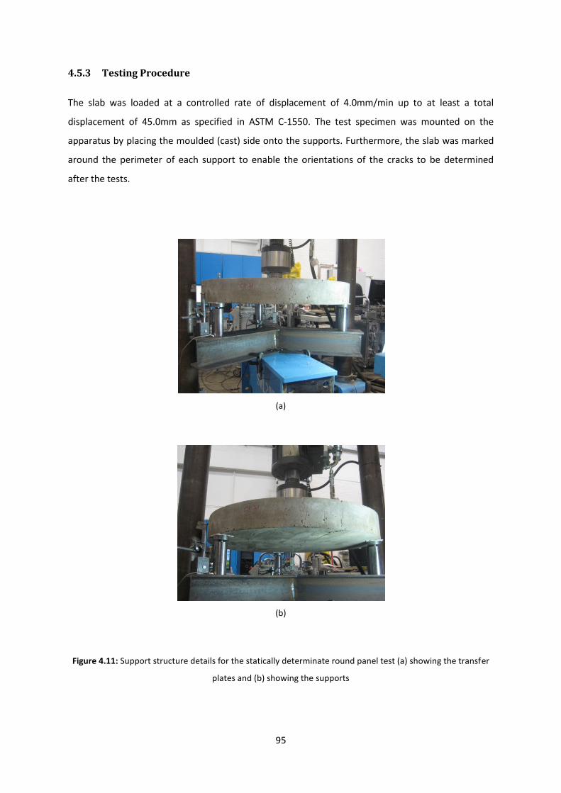
95
4.5.3 Testing Procedure
The slab was loaded at a controlled rate of displacement of 4.0mm/min up to at least a total
displacement of 45.0mm as specified in ASTM C-1550. The test specimen was mounted on the
apparatus by placing the moulded (cast) side onto the supports. Furthermore, the slab was marked
around the perimeter of each support to enable the orientations of the cracks to be determined
after the tests.
(a)
(b)
Figure 4.11: Support structure details for the statically determinate round panel test (a) showing the transfer
plates and (b) showing the supports
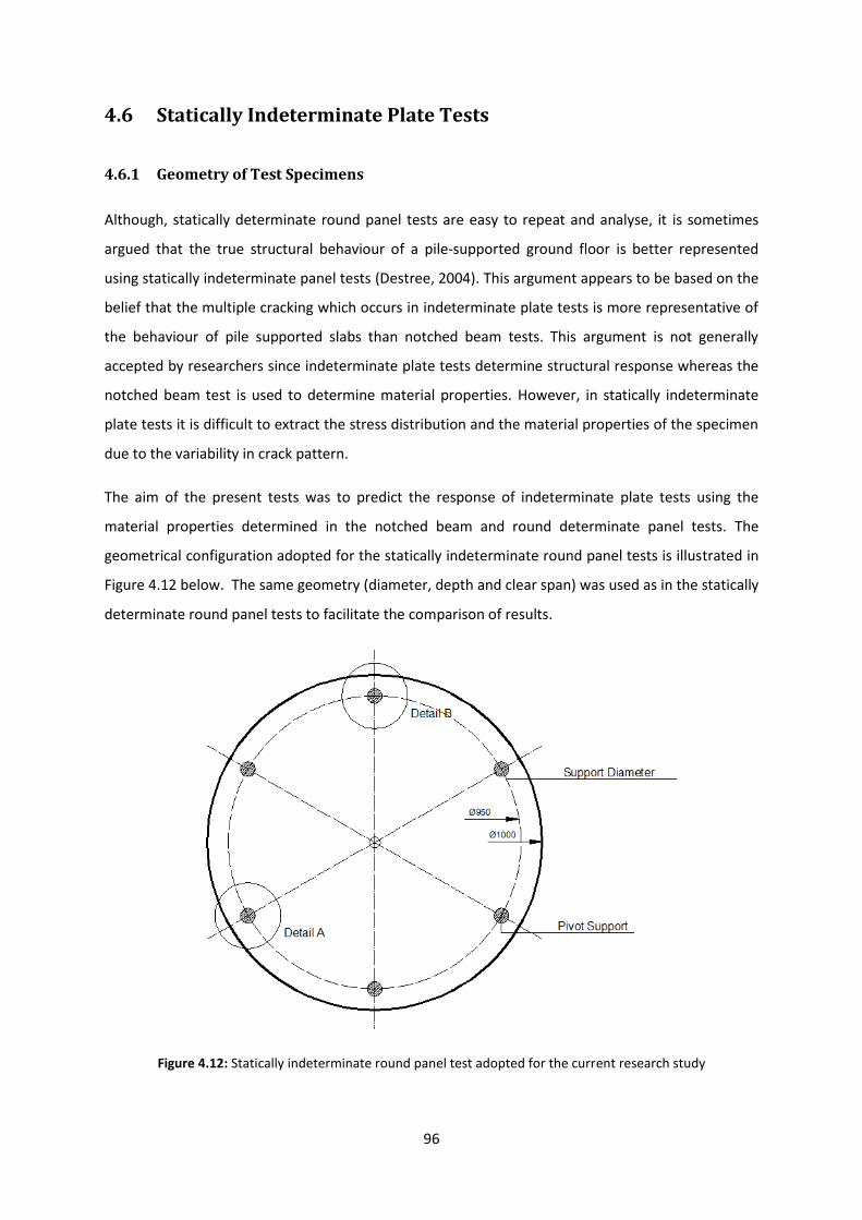
96
4.6 Statically Indeterminate Plate Tests
4.6.1 Geometry of Test Specimens
Although, statically determinate round panel tests are easy to repeat and analyse, it is sometimes
argued that the true structural behaviour of a pile-supported ground floor is better represented
using statically indeterminate panel tests (Destree, 2004). This argument appears to be based on the
belief that the multiple cracking which occurs in indeterminate plate tests is more representative of
the behaviour of pile supported slabs than notched beam tests. This argument is not generally
accepted by researchers since indeterminate plate tests determine structural response whereas the
notched beam test is used to determine material properties. However, in statically indeterminate
plate tests it is difficult to extract the stress distribution and the material properties of the specimen
due to the variability in crack pattern.
The aim of the present tests was to predict the response of indeterminate plate tests using the
material properties determined in the notched beam and round determinate panel tests. The
geometrical configuration adopted for the statically indeterminate round panel tests is illustrated in
Figure 4.12 below. The same geometry (diameter, depth and clear span) was used as in the statically
determinate round panel tests to facilitate the comparison of results.
Figure 4.12: Statically indeterminate round panel test adopted for the current research study
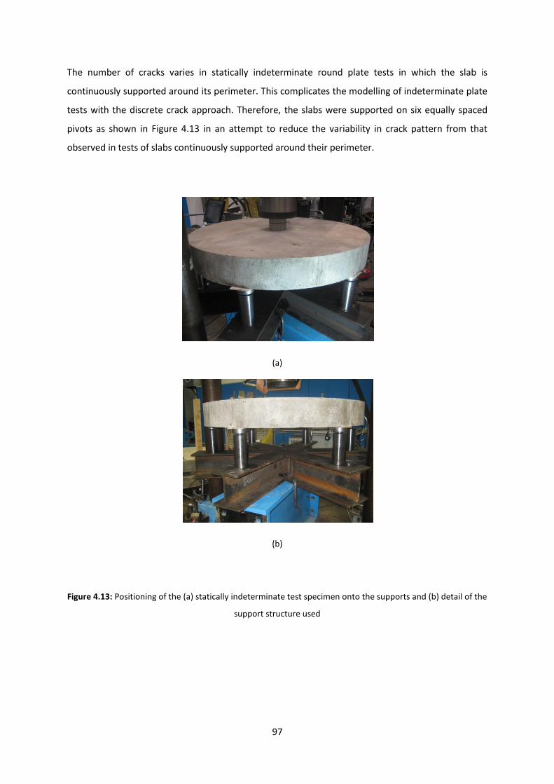
97
The number of cracks varies in statically indeterminate round plate tests in which the slab is
continuously supported around its perimeter. This complicates the modelling of indeterminate plate
tests with the discrete crack approach. Therefore, the slabs were supported on six equally spaced
pivots as shown in Figure 4.13 in an attempt to reduce the variability in crack pattern from that
observed in tests of slabs continuously supported around their perimeter.
(a)
(b)
Figure 4.13: Positioning of the (a) statically indeterminate test specimen onto the supports and (b) detail of the
support structure used

98
(a)
(b)
(c)
Figure 4.14: LVDT used to (a) measure the vertical displacement (b) the bedding – in of the steel support (c)
the deflection of the support structure relative to the laboratory floor

99
4.6.2 Instrumentation and Testing
The instrumentation in the statically indeterminate round plate tests was similar to that used in the
round determinate plate tests, which is described in Section 4.5.2. The effects of friction were
minimised by placing a 0.5mm thick layer of PTFE between the round base plate and the supports
which were identical to those used in the round determinate plate test (see Figures 4.9 and 4.10).
The load was imposed at a controlled rate of displacement of 4.0mm/min up to a total displacement
of 45mm as in the round determinate plate tests. In order to ensure that all supports were in
contact, the specimen was initially placed onto the three supports. Subsequently, the remaining
three supports were raised until they came into contact with the specimen.
4.6 Crack widths in Round Determinate Panel Tests
4.6.1 Test setup
As highlighted in the literature review, pile-supported slabs can, in some cases, suffer from
serviceability issues such as excessive cracking. An innovative test setup has been devised in order to
relate the crack width to the displacement, as part of the present research. It is not practical to
measure crack widths in the standard ASTM C-1550 test setup due to the difficulty of accessing the
underside of the specimen.
Therefore, it was decided to ‘reverse’ the loading arrangement as shown in Figure 4.15.
Consequently, the slab was supported at its centre as shown in Figure 4.16 and loaded from the top
through a three armed ‘spider’.
This test setup was adopted in order to have the cracks occurring at the top rather than the bottom
surface. This allowed crack widths to be measured during the experiment using both Demec gauges
and transducers. A more detailed description of the instrumentation used for this phase is given in
Section 4.6.2.
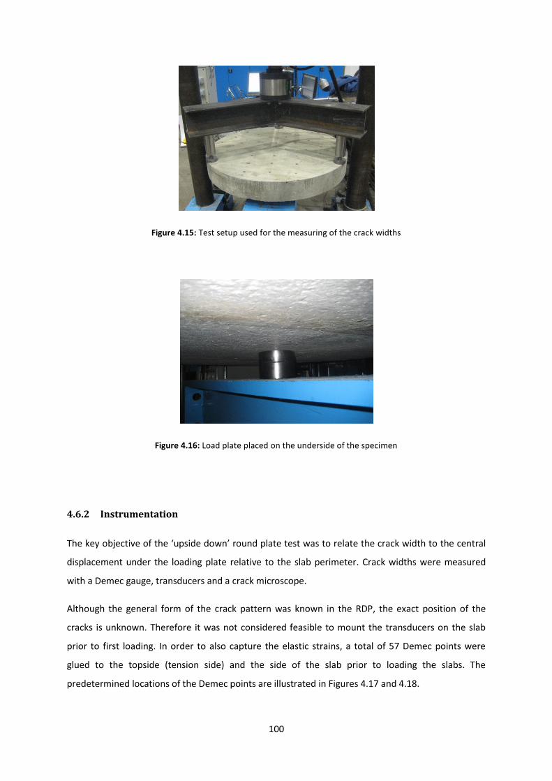
100
Figure 4.15: Test setup used for the measuring of the crack widths
Figure 4.16: Load plate placed on the underside of the specimen
4.6.2 Instrumentation
The key objective of the ‘upside down’ round plate test was to relate the crack width to the central
displacement under the loading plate relative to the slab perimeter. Crack widths were measured
with a Demec gauge, transducers and a crack microscope.
Although the general form of the crack pattern was known in the RDP, the exact position of the
cracks is unknown. Therefore it was not considered feasible to mount the transducers on the slab
prior to first loading. In order to also capture the elastic strains, a total of 57 Demec points were
glued to the topside (tension side) and the side of the slab prior to loading the slabs. The
predetermined locations of the Demec points are illustrated in Figures 4.17 and 4.18.

101
Figure 4.17: Demec points on the topside (tension side) of the specimen in question
Figure 4.18: Positioning of Demec points and Demec point reading references
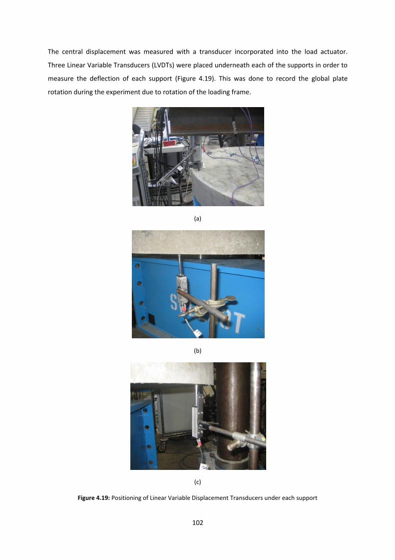
102
The central displacement was measured with a transducer incorporated into the load actuator.
Three Linear Variable Transducers (LVDTs) were placed underneath each of the supports in order to
measure the deflection of each support (Figure 4.19). This was done to record the global plate
rotation during the experiment due to rotation of the loading frame.
(a)
(b)
(c)
Figure 4.19: Positioning of Linear Variable Displacement Transducers under each support
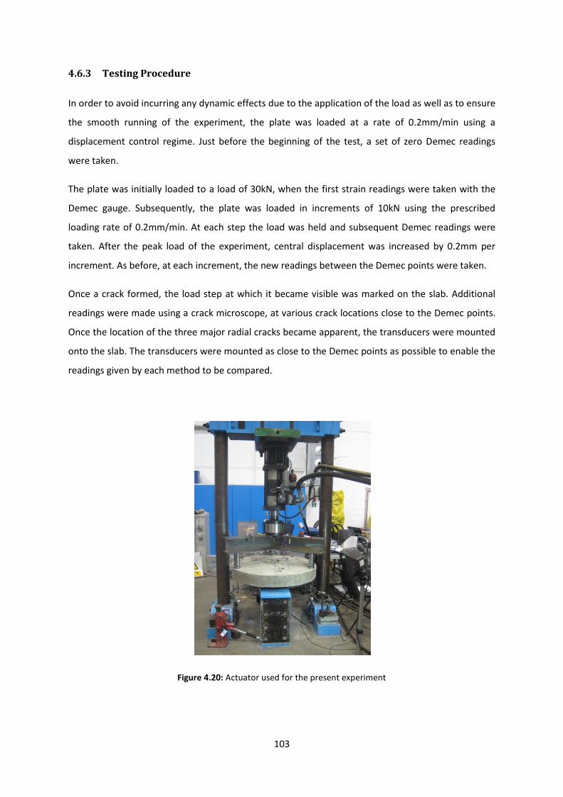
103
4.6.3 Testing Procedure
In order to avoid incurring any dynamic effects due to the application of the load as well as to ensure
the smooth running of the experiment, the plate was loaded at a rate of 0.2mm/min using a
displacement control regime. Just before the beginning of the test, a set of zero Demec readings
were taken.
The plate was initially loaded to a load of 30kN, when the first strain readings were taken with the
Demec gauge. Subsequently, the plate was loaded in increments of 10kN using the prescribed
loading rate of 0.2mm/min. At each step the load was held and subsequent Demec readings were
taken. After the peak load of the experiment, central displacement was increased by 0.2mm per
increment. As before, at each increment, the new readings between the Demec points were taken.
Once a crack formed, the load step at which it became visible was marked on the slab. Additional
readings were made using a crack microscope, at various crack locations close to the Demec points.
Once the location of the three major radial cracks became apparent, the transducers were mounted
onto the slab. The transducers were mounted as close to the Demec points as possible to enable the
readings given by each method to be compared.
Figure 4.20: Actuator used for the present experiment

104
4.7 Damaged Determinate Round Panel Tests under Reloading
4.7.1 Test setup
Pile supported ground floors are frequently subjected to loading and unloading of racks or shelves
and the movement of heavy goods vehicles. This can amount to hundreds of thousands of loading
and unloading cycles during the slab’s service life. The formation and propagation of cracks can
impair the performance of a pile supported slab during its service life. Although a number of
measures, such as minimising in plane restraint and the use of low shrinkage concretes, can be taken
to minimise or eliminate surface cracking, there are many instances where cracking occurs.
The present test considers the behaviour of a damaged pile supported slab under repeated
reloading. The tests are intended to give an indication of the residual stiffness and strength of
damaged SFRC slabs under extreme loading rather than information on fatigue which would require
an order of magnitude more load cycles. The test setup of the present experiment was identical with
the one described in Section 4.6.2 of the present chapter. The instrumentation of this test was
identical with that described in Section 4.6.3.
4.7.2 Testing Procedure
The slab was loaded up to the peak load in increments of 10kN per time at a loading rate of
0.2mm/min. At each increment (load step) the crack positions were marked and crack widths were
measured with the Demec gauge.
Once the locations of the three major radial cracks became apparent, a total of nine transducers
(three on each crack) were mounted. The transducers were mounted relatively close to the Demec
gauges, so that the number of readings obtained overlapped as described previously in section 4.6.3.
After the transducers were mounted, the slab was unloaded and re-loaded in three cycles. At the
first and last loading/unloading Demec readings were also taken. After this initial loading the slab
was loaded up to an approximate crack width of 1mm, where it was unloaded and loaded again
three times. The same sequence was repeated when the crack width reached to a crack width of
about 1.5mm.
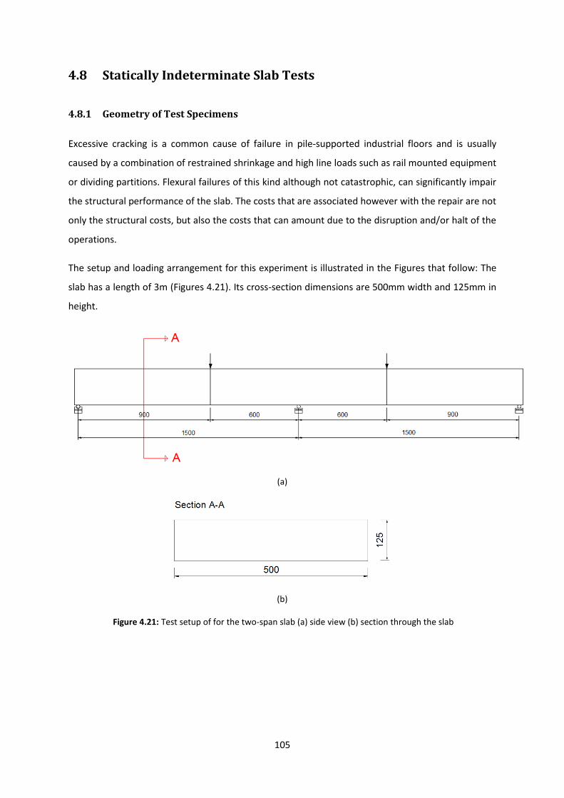
105
4.8 Statically Indeterminate Slab Tests
4.8.1 Geometry of Test Specimens
Excessive cracking is a common cause of failure in pile-supported industrial floors and is usually
caused by a combination of restrained shrinkage and high line loads such as rail mounted equipment
or dividing partitions. Flexural failures of this kind although not catastrophic, can significantly impair
the structural performance of the slab. The costs that are associated however with the repair are not
only the structural costs, but also the costs that can amount due to the disruption and/or halt of the
operations.
The setup and loading arrangement for this experiment is illustrated in the Figures that follow: The
slab has a length of 3m (Figures 4.21). Its cross-section dimensions are 500mm width and 125mm in
height.
(a)
(b)
Figure 4.21: Test setup of for the two-span slab (a) side view (b) section through the slab
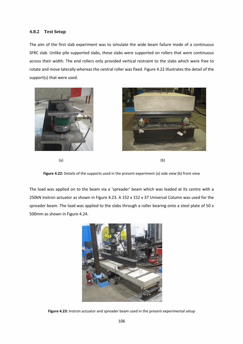
106
4.8.2 Test Setup
The aim of the first slab experiment was to simulate the wide beam failure mode of a continuous
SFRC slab. Unlike pile supported slabs, these slabs were supported on rollers that were continuous
across their width. The end rollers only provided vertical restraint to the slabs which were free to
rotate and move laterally whereas the central roller was fixed. Figure 4.22 illustrates the detail of the
support(s) that were used.
(a) (b)
Figure 4.22: Details of the supports used in the present experiment (a) side view (b) front view
The load was applied on to the beam via a ‘spreader’ beam which was loaded at its centre with a
250kN Instron actuator as shown in Figure 4.23. A 152 x 152 x 37 Universal Column was used for the
spreader beam. The load was applied to the slabs through a roller bearing onto a steel plate of 50 x
500mm as shown in Figure 4.24.
Figure 4.23: Instron actuator and spreader beam used in the present experimental setup
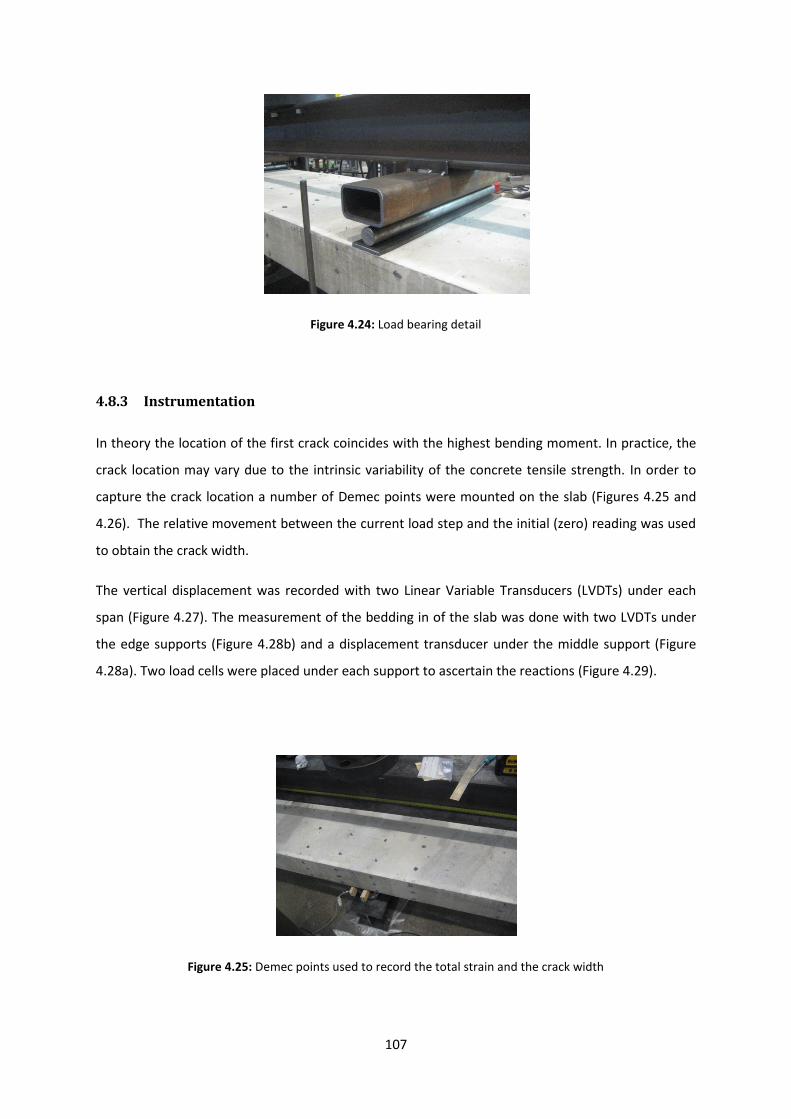
107
Figure 4.24: Load bearing detail
4.8.3 Instrumentation
In theory the location of the first crack coincides with the highest bending moment. In practice, the
crack location may vary due to the intrinsic variability of the concrete tensile strength. In order to
capture the crack location a number of Demec points were mounted on the slab (Figures 4.25 and
4.26). The relative movement between the current load step and the initial (zero) reading was used
to obtain the crack width.
The vertical displacement was recorded with two Linear Variable Transducers (LVDTs) under each
span (Figure 4.27). The measurement of the bedding in of the slab was done with two LVDTs under
the edge supports (Figure 4.28b) and a displacement transducer under the middle support (Figure
4.28a). Two load cells were placed under each support to ascertain the reactions (Figure 4.29).
Figure 4.25: Demec points used to record the total strain and the crack width
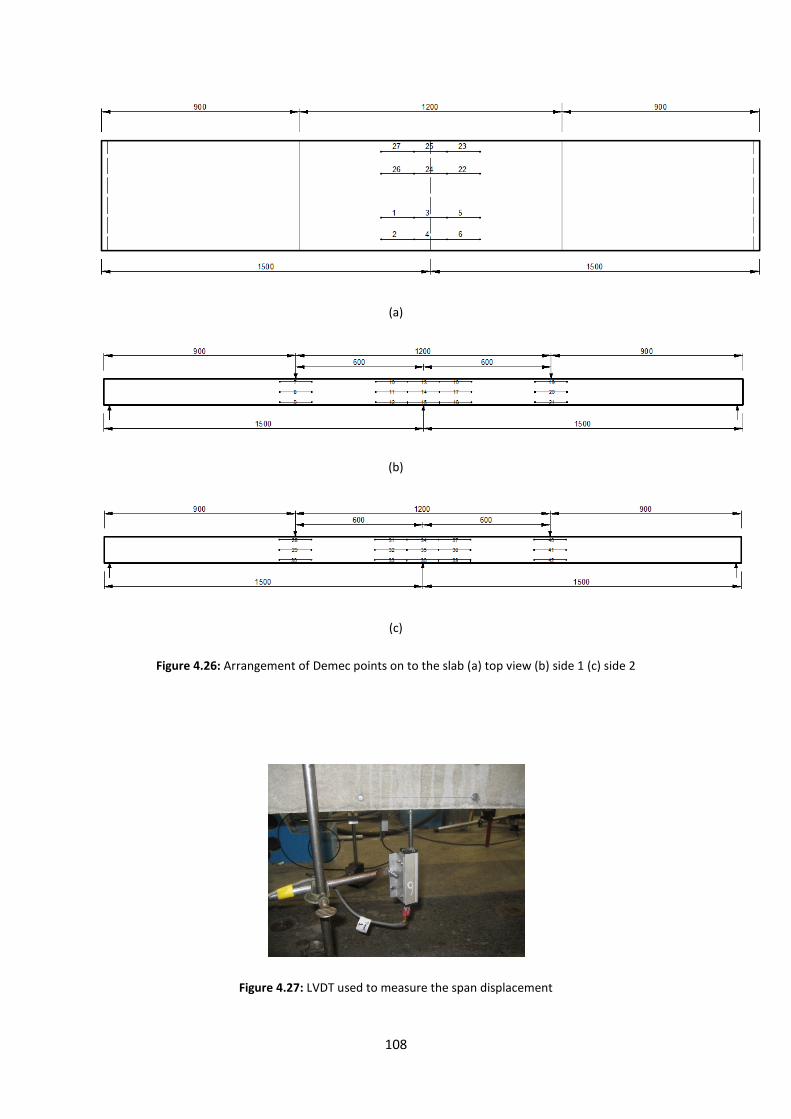
108
(a)
(b)
(c)
Figure 4.26: Arrangement of Demec points on to the slab (a) top view (b) side 1 (c) side 2
Figure 4.27: LVDT used to measure the span displacement
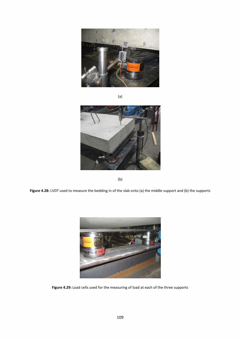
109
(a)
(b)
Figure 4.28: LVDT used to measure the bedding in of the slab onto (a) the middle support and (b) the supports
Figure 4.29: Load cells used for the measuring of load at each of the three supports
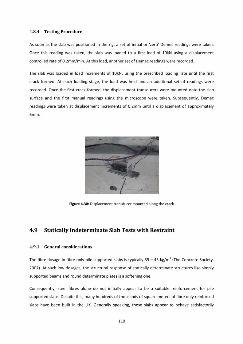
110
4.8.4 Testing Procedure
As soon as the slab was positioned in the rig, a set of initial or ‘zero’ Demec readings were taken.
Once this reading was taken, the slab was loaded to a first load of 10kN using a displacement
controlled rate of 0.2mm/min. At this load, another set of Demec readings were recorded.
The slab was loaded in load increments of 10kN, using the prescribed loading rate until the first
crack formed. At each loading stage, the load was held and an additional set of readings were
recorded. Once the first crack formed, the displacement transducers were mounted onto the slab
surface and the first manual readings using the microscope were taken. Subsequently, Demec
readings were taken at displacement increments of 0.2mm until a displacement of approximately
6mm.
Figure 4.30: Displacement transducer mounted along the crack
4.9 Statically Indeterminate Slab Tests with Restraint
4.9.1 General considerations
The fibre dosage in fibre-only pile-supported slabs is typically 35 – 45 kg/m3 (The Concrete Society,
2007). At such low dosages, the structural response of statically determinate structures like simply
supported beams and round determinate plates is a softening one.
Consequently, steel fibres alone do not initially appear to be a suitable reinforcement for pile
supported slabs. Despite this, many hundreds of thousands of square meters of fibre only reinforced
slabs have been built in the UK. Generally speaking, these slabs appear to behave satisfactorily
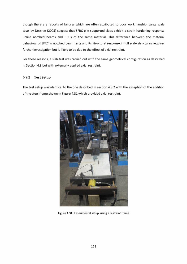
111
though there are reports of failures which are often attributed to poor workmanship. Large scale
tests by Destree (2005) suggest that SFRC pile supported slabs exhibit a strain hardening response
unlike notched beams and RDPs of the same material. This difference between the material
behaviour of SFRC in notched beam tests and its structural response in full scale structures requires
further investigation but is likely to be due to the effect of axial restraint.
For these reasons, a slab test was carried out with the same geometrical configuration as described
in Section 4.8 but with externally applied axial restraint.
4.9.2 Test Setup
The test setup was identical to the one described in section 4.8.2 with the exception of the addition
of the steel frame shown in Figure 4.31 which provided axial restraint.
Figure 4.31: Experimental setup, using a restraint frame
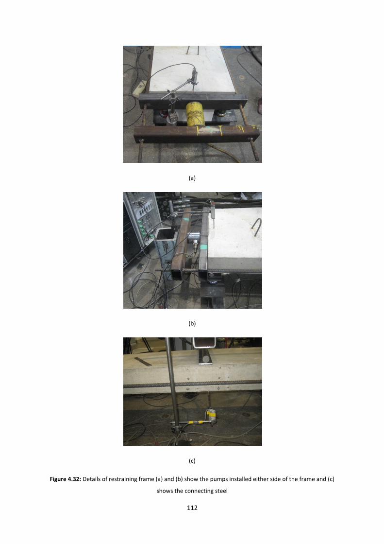
112
(a)
(b)
(c)
Figure 4.32: Details of restraining frame (a) and (b) show the pumps installed either side of the frame and (c)
shows the connecting steel
113
A manually controlled hydraulic actuator was used to apply and maintain an axial load to the slab as
shown in Figures 4.32 (a) and (b). The slab was loaded through an internal reaction frame that
consisted of two hollow steel sections tied together with two H16 reinforcement bars.
4.9.3 Instrumentation and Testing Procedure
The instrumentation used for the present experiment was identical to the one described in section
4.8.3, with the sole exception that a separate data scan unit was used to record the axial
compressive force applied to the slab.
The load was increased in increments of 10kN until the first crack formed. A set of Demec readings
was taken after each load increment. As soon as the exact locations of the cracks became apparent,
the displacement transducers were mounted into the slab. Demec readings continued to be taken in
order to ensure adequate overlap between these two methods of instrumentation. As soon as the
load started decreasing, the axial restraint was increased to 5kN. At this point, the displacement was
held and another set of Demec readings was taken. After this step, the displacement was increased
in increments of 0.5mm, always maintaining the same loading rate of 0.2mm/min.
4.10 Punching Shear Tests
4.10.1 General considerations
An additional set of sets was undertaken on behalf of Abbey Pynford to investigate the flexural and
punching shear resistance of SFRC. Four sets of round panel tests were carried out as described
below. All the plates were 125m thick with a diameter of 1m as described previously. The concrete
mix details have been omitted at the request of Abbey Pynford.
Cast 1 was a plain concrete mix. This mix was used as a benchmark with which the effect of the
steel fibres could be assessed against.
In Cast 2, Arcelor Mittal He-75-35 steel fibres were added at a dosage of 50kg/m3. These are
35mm long hooked fibres with a 0.75mm diameter and an aspect ratio of 47. The tensile
strength of the fibres was 1200MPa.
Cast 3 incorporated Arcelor Mittal He-55-35 steel fibres at a dosage of 50kg/m3. These are
35mm long hooked fibres with a 0.55mm diameter and an aspect ratio of 64. The tensile
strength of the fibres was 1200MPa.
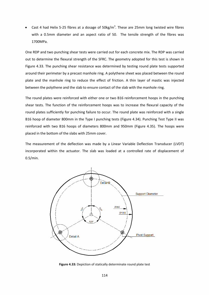
114
Cast 4 had Helix 5-25 fibres at a dosage of 50kg/m3. These are 25mm long twisted wire fibres
with a 0.5mm diameter and an aspect ratio of 50. The tensile strength of the fibres was
1700MPa.
One RDP and two punching shear tests were carried out for each concrete mix. The RDP was carried
out to determine the flexural strength of the SFRC. The geometry adopted for this test is shown in
Figure 4.33. The punching shear resistance was determined by testing round plate tests supported
around their perimeter by a precast manhole ring. A polythene sheet was placed between the round
plate and the manhole ring to reduce the effect of friction. A thin layer of mastic was injected
between the polythene and the slab to ensure contact of the slab with the manhole ring.
The round plates were reinforced with either one or two B16 reinforcement hoops in the punching
shear tests. The function of the reinforcement hoops was to increase the flexural capacity of the
round plates sufficiently for punching failure to occur. The round plate was reinforced with a single
B16 hoop of diameter 800mm in the Type I punching tests (Figure 4.34). Punching Test Type II was
reinforced with two B16 hoops of diameters 800mm and 950mm (Figure 4.35). The hoops were
placed in the bottom of the slabs with 25mm cover.
The measurement of the deflection was made by a Linear Variable Deflection Transducer (LVDT)
incorporated within the actuator. The slab was loaded at a controlled rate of displacement of
0.5/min.
Figure 4.33: Depiction of statically determinate round plate test

115
Figure 4.34: Depiction of punching test type 1, with a single B16 hoop
Figure 4.35: Depiction of punching test type 2, with two B16 hoops
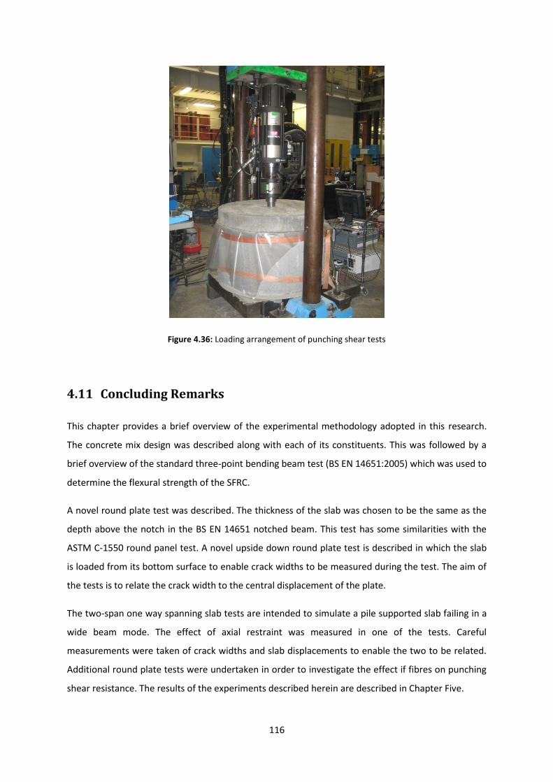
116
Figure 4.36: Loading arrangement of punching shear tests
4.11 Concluding Remarks
This chapter provides a brief overview of the experimental methodology adopted in this research.
The concrete mix design was described along with each of its constituents. This was followed by a
brief overview of the standard three-point bending beam test (BS EN 14651:2005) which was used to
determine the flexural strength of the SFRC.
A novel round plate test was described. The thickness of the slab was chosen to be the same as the
depth above the notch in the BS EN 14651 notched beam. This test has some similarities with the
ASTM C-1550 round panel test. A novel upside down round plate test is described in which the slab
is loaded from its bottom surface to enable crack widths to be measured during the test. The aim of
the tests is to relate the crack width to the central displacement of the plate.
The two-span one way spanning slab tests are intended to simulate a pile supported slab failing in a
wide beam mode. The effect of axial restraint was measured in one of the tests. Careful
measurements were taken of crack widths and slab displacements to enable the two to be related.
Additional round plate tests were undertaken in order to investigate the effect if fibres on punching
shear resistance. The results of the experiments described herein are described in Chapter Five.
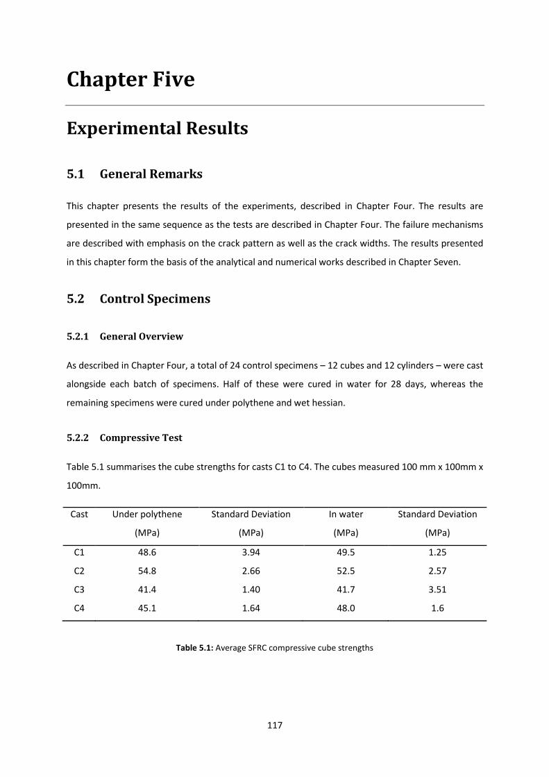
117
Chapter Five
Experimental Results
5.1 General Remarks
This chapter presents the results of the experiments, described in Chapter Four. The results are
presented in the same sequence as the tests are described in Chapter Four. The failure mechanisms
are described with emphasis on the crack pattern as well as the crack widths. The results presented
in this chapter form the basis of the analytical and numerical works described in Chapter Seven.
5.2 Control Specimens
5.2.1 General Overview
As described in Chapter Four, a total of 24 control specimens – 12 cubes and 12 cylinders – were cast
alongside each batch of specimens. Half of these were cured in water for 28 days, whereas the
remaining specimens were cured under polythene and wet hessian.
5.2.2 Compressive Test
Table 5.1 summarises the cube strengths for casts C1 to C4. The cubes measured 100 mm x 100mm x
100mm.
Cast Under polythene
(MPa)
Standard Deviation
(MPa)
In water
(MPa)
Standard Deviation
(MPa)
C1 48.6 3.94 49.5 1.25
C2 54.8 2.66 52.5 2.57
C3 41.4 1.40 41.7 3.51
C4 45.1 1.64 48.0 1.6
Table 5.1: Average SFRC compressive cube strengths
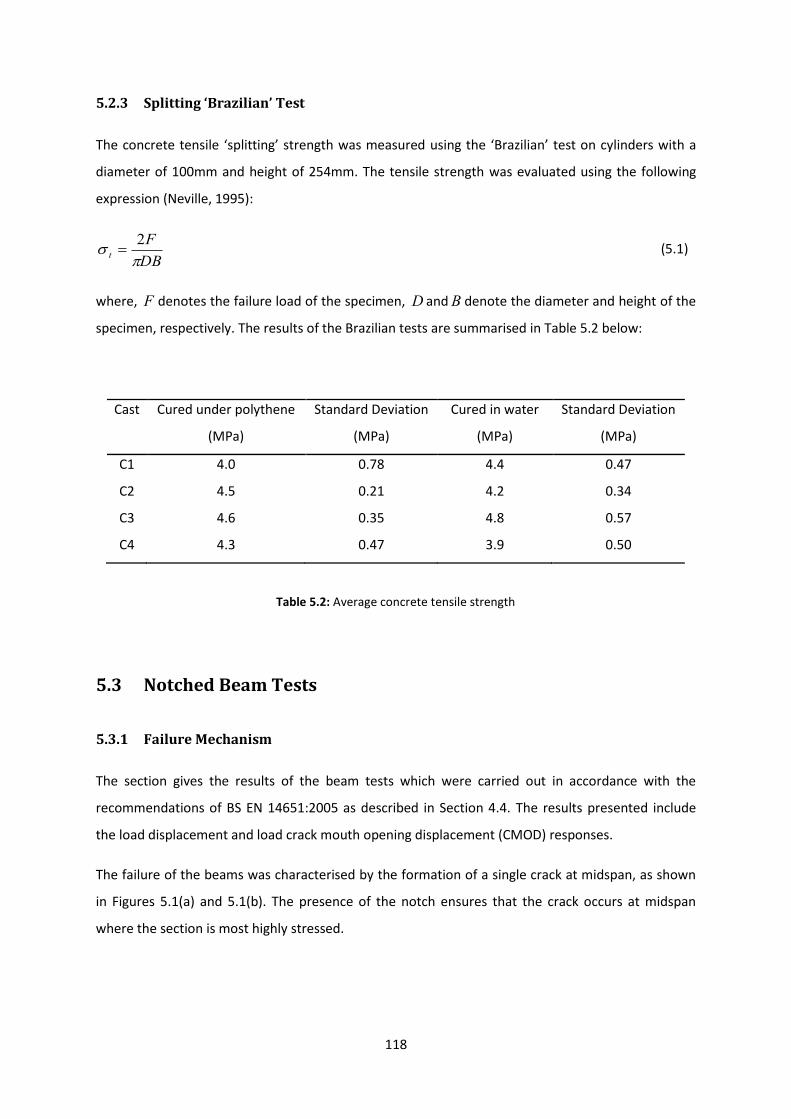
118
5.2.3 Splitting ‘Brazilian’ Test
The concrete tensile ‘splitting’ strength was measured using the ‘Brazilian’ test on cylinders with a
diameter of 100mm and height of 254mm. The tensile strength was evaluated using the following
expression (Neville, 1995):
DB
Ft
2 (5.1)
where, F denotes the failure load of the specimen, D andB denote the diameter and height of the
specimen, respectively. The results of the Brazilian tests are summarised in Table 5.2 below:
Cast Cured under polythene
(MPa)
Standard Deviation
(MPa)
Cured in water
(MPa)
Standard Deviation
(MPa)
C1 4.0 0.78 4.4 0.47
C2 4.5 0.21 4.2 0.34
C3 4.6 0.35 4.8 0.57
C4 4.3 0.47 3.9 0.50
Table 5.2: Average concrete tensile strength
5.3 Notched Beam Tests
5.3.1 Failure Mechanism
The section gives the results of the beam tests which were carried out in accordance with the
recommendations of BS EN 14651:2005 as described in Section 4.4. The results presented include
the load displacement and load crack mouth opening displacement (CMOD) responses.
The failure of the beams was characterised by the formation of a single crack at midspan, as shown
in Figures 5.1(a) and 5.1(b). The presence of the notch ensures that the crack occurs at midspan
where the section is most highly stressed.

119
(a)
(b)
Figure 5.1: Failure mode of three point bending beam with a single crack
5.3.3 Load – Deflection Response
EN 14651:2005 gives the option of either recording the load-deflection or the load – CMOD
response. For the purpose of the present research both responses were measured. Figures 5.2 to 5.5
give the load – deflection responses for each of the four sets of beams tested.
The load-deflection response of the SFRC beams under three point bending is characterised by three
distinct phases. Before cracking the response is linear. The cracking load is a function of the concrete
tensile strength and fibre dosage (Tlemat, Pilakoutas, & Neocleous, 2006). The fibre geometry has
very little effect on the load (Banthia & Trottier, 1994). The second phase is triggered by crack
formation and propagation. During this phase, the beam reached its peak load. Subsequently, the
load typically dropped as the fibre dosage of 45 kg/m3 was insufficient to maintain the peak load
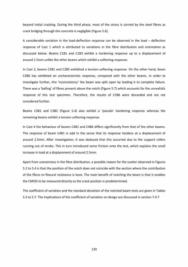
120
beyond initial cracking. During the third phase, most of the stress is carried by the steel fibres as
crack bridging through the concrete is negligible (Figure 5.6).
A considerable variation in the load-deflection response can be observed in the load – deflection
response of Cast 1 which is attributed to variations in the fibre distribution and orientation as
discussed below. Beams C1B1 and C1B3 exhibit a hardening response up to a displacement of
around 1.5mm unlike the other beams which exhibit a softening response.
In Cast 2, beams C2B1 and C2B5 exhibited a tension softening response. On the other hand, beam
C2B6 has exhibited an uncharacteristic response, compared with the other beams. In order to
investigate further, this ‘inconsistency’ the beam was split open by loading it to complete failure.
There was a ‘balling’ of fibres present above the notch (Figure 5.7) which accounts for the unrealistic
response of this test specimen. Therefore, the results of C2B6 were discarded and are not
considered further.
Beams C3B1 and C3B2 (Figure 5.4) also exhibit a ‘pseudo’ hardening response whereas the
remaining beams exhibit a tension softening response.
In Cast 4 the behaviour of beams C4B1 and C4B6 differs significantly from that of the other beams.
The response of beam C4B1 is odd in the sense that its response hardens at a displacement of
around 2.5mm. After investigation, it was deduced that this occurred due to the support rollers
running out of stroke. This in turn introduced some friction onto the test, which explains the small
increase in load at a displacement of around 2.5mm.
Apart from unevenness in the fibre distribution, a possible reason for the scatter observed in Figures
5.2 to 5.4 is that the position of the notch does not coincide with the section where the contribution
of the fibres to flexural resistance is least. The main benefit of notching the beam is that it enables
the CMOD to be measured directly as the crack position is predetermined.
The coefficient of variation and the standard deviation of the notched beam tests are given in Tables
5.3 to 5.7. The implications of the coefficient of variation on design are discussed in section 7.4.7

121
Figure 5.2: Three point bending beam load – deflection response for Cast 1
Figure 5.3: Three point bending beam load – deflection response for Cast 2
0
4
8
12
16
20
0 1 2 3 4 5 6
Load
(kN
)
Displacement (mm)
C1B1 C1B2
C1B3 C1B4
C1B5 C1B6
Average
0
5
10
15
20
25
30
0 1 2 3 4 5 6
Load
(kN
)
Displacement (mm)
C2B1 C2B2
C2B3 C2B4
C2B5 C2B6
Average

122
Figure 5.4: Three point bending beam load – deflection response for Cast 3
Figure 5.5: Three point bending beam load – deflection response for Cast 4
0
5
10
15
20
25
0 1 2 3 4 5 6
Load
(kN
)
Displacement (mm)
C3B1 C3B2
C3B3 C3B4
C3B5 C3B6
Average
0
5
10
15
20
25
0 1 2 3 4 5 6
Load
(kN
)
Displacement (mm)
C4B1 C4B2
C4B3 C4B4
C4B5 C4B6
Average
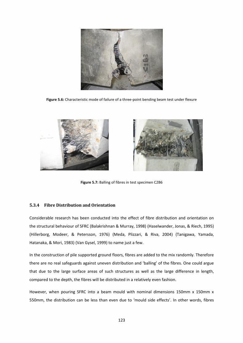
123
Figure 5.6: Characteristic mode of failure of a three-point bending beam test under flexure
Figure 5.7: Balling of fibres in test specimen C2B6
5.3.4 Fibre Distribution and Orientation
Considerable research has been conducted into the effect of fibre distribution and orientation on
the structural behaviour of SFRC (Balakrishnan & Murray, 1998) (Haselwander, Jonas, & Riech, 1995)
(Hillerborg, Modeer, & Petersson, 1976) (Meda, Plizzari, & Riva, 2004) (Tanigawa, Yamada,
Hatanaka, & Mori, 1983) (Van Gysel, 1999) to name just a few.
In the construction of pile supported ground floors, fibres are added to the mix randomly. Therefore
there are no real safeguards against uneven distribution and ‘balling’ of the fibres. One could argue
that due to the large surface areas of such structures as well as the large difference in length,
compared to the depth, the fibres will be distributed in a relatively even fashion.
However, when pouring SFRC into a beam mould with nominal dimensions 150mm x 150mm x
550mm, the distribution can be less than even due to ‘mould side effects’. In other words, fibres
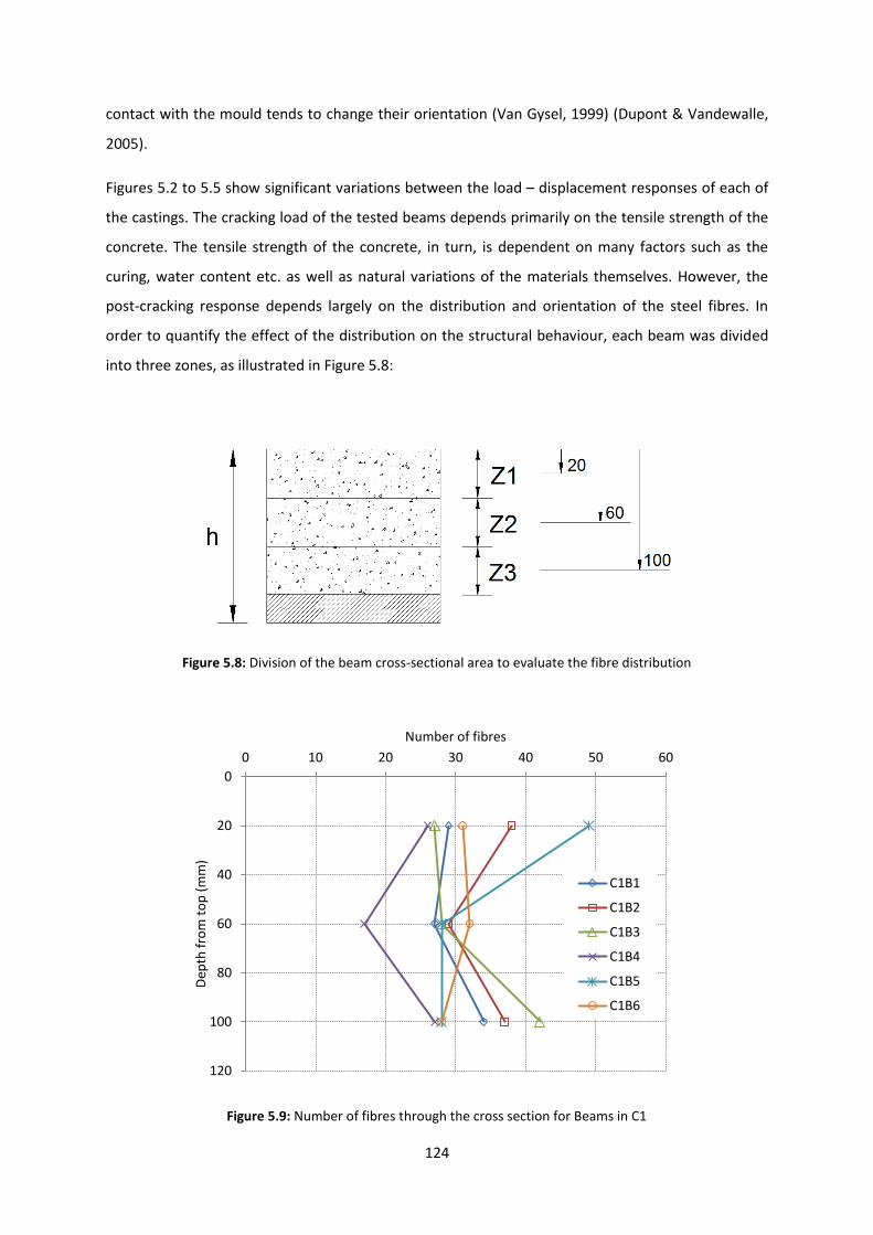
124
contact with the mould tends to change their orientation (Van Gysel, 1999) (Dupont & Vandewalle,
2005).
Figures 5.2 to 5.5 show significant variations between the load – displacement responses of each of
the castings. The cracking load of the tested beams depends primarily on the tensile strength of the
concrete. The tensile strength of the concrete, in turn, is dependent on many factors such as the
curing, water content etc. as well as natural variations of the materials themselves. However, the
post-cracking response depends largely on the distribution and orientation of the steel fibres. In
order to quantify the effect of the distribution on the structural behaviour, each beam was divided
into three zones, as illustrated in Figure 5.8:
Figure 5.8: Division of the beam cross-sectional area to evaluate the fibre distribution
Figure 5.9: Number of fibres through the cross section for Beams in C1
0
20
40
60
80
100
120
0 10 20 30 40 50 60
Dep
th f
rom
to
p (
mm
)
Number of fibres
C1B1
C1B2
C1B3
C1B4
C1B5
C1B6
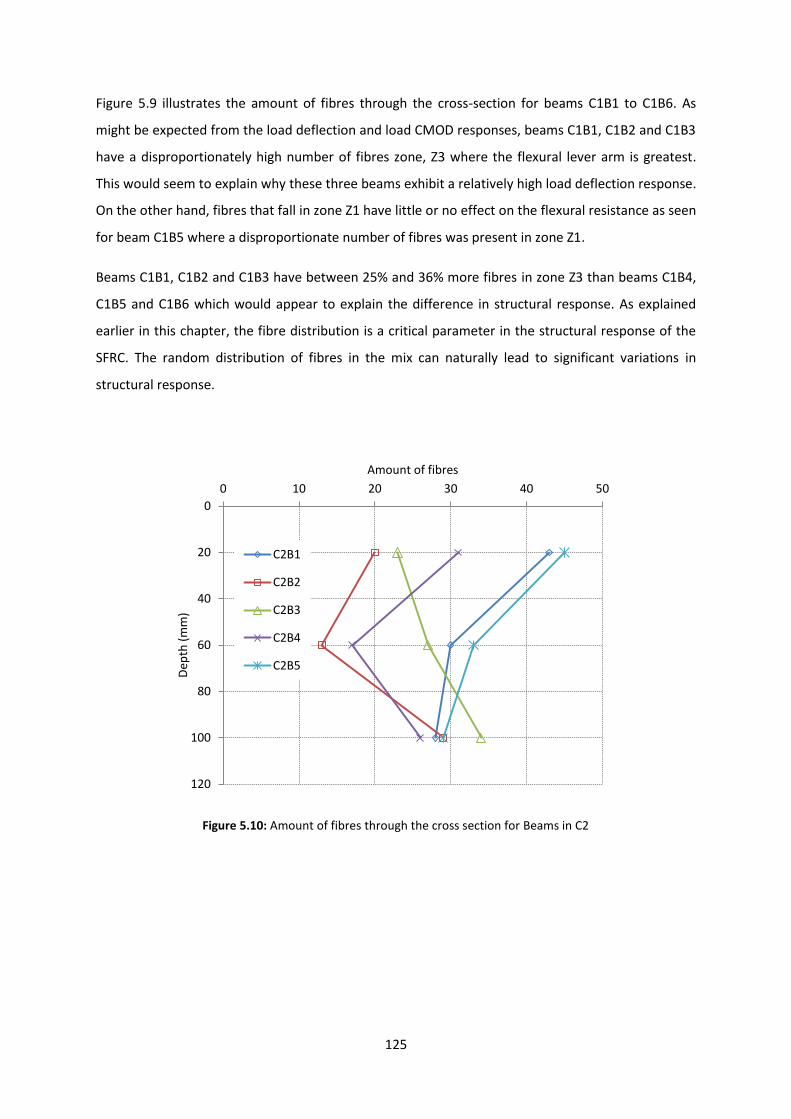
125
Figure 5.9 illustrates the amount of fibres through the cross-section for beams C1B1 to C1B6. As
might be expected from the load deflection and load CMOD responses, beams C1B1, C1B2 and C1B3
have a disproportionately high number of fibres zone, Z3 where the flexural lever arm is greatest.
This would seem to explain why these three beams exhibit a relatively high load deflection response.
On the other hand, fibres that fall in zone Z1 have little or no effect on the flexural resistance as seen
for beam C1B5 where a disproportionate number of fibres was present in zone Z1.
Beams C1B1, C1B2 and C1B3 have between 25% and 36% more fibres in zone Z3 than beams C1B4,
C1B5 and C1B6 which would appear to explain the difference in structural response. As explained
earlier in this chapter, the fibre distribution is a critical parameter in the structural response of the
SFRC. The random distribution of fibres in the mix can naturally lead to significant variations in
structural response.
Figure 5.10: Amount of fibres through the cross section for Beams in C2
0
20
40
60
80
100
120
0 10 20 30 40 50
Dep
th (
mm
)
Amount of fibres
C2B1
C2B2
C2B3
C2B4
C2B5

126
Figure 5.11: Amount of fibres through the cross section for Beams in C3
Unlike Cast C1, in Cast C2 the load – displacement response seems to be somewhat more consistent
with the exception of beam C2B3. The response of beam C2B6 has been discarded, as stated
previously due to the balling of fibres which exaggerated its behaviour. All the beams, with the
exception of C2B3 have a nearly identical number of fibres in zone Z3 which contributes most to
flexural resistance. This is consistent with the uniformity of the structural response. On the other
hand beam C2B3 had around 15% more fibres in the tensile zone than the rest of the specimens.
Figure 5.11 illustrates the fibre distribution counted in Cast C3. From the load deflection response
obtained (Figure 5.4) one can observe the difference in behaviour between beams C3B1 C3B2 and
the rest. C3B1 and B2 exhibit a somewhat stiffer response which, like in the previous cases, can be
partially explained by the distribution of steel fibres through the cross section. Beam C3B1 shows the
highest amount of steel fibres in the bottom third, along with beam C3B4. Although the fibre
contents of these two beams appear at a first glance to be similar, the actual dispersion is somewhat
different which could explain the differing structural responses of each. In the cross-section of beam
C3B4 one can observe that the fibres in the bottom third are dispersed towards one side of the
beam leaving the other totally ‘unreinforced’ (Figure 5.12b). This effect although present is much
less noticeable in beam C3B2 which may explain the difference in response.
Figure 5.13 illustrates the results of the fibre counting exercise for casting C4, the load-displacement
results of which are presented in Figure 5.5. The structural behaviour of the six beams seems to be
0
20
40
60
80
100
120
0 10 20 30 40 50 60
Dep
th (
mm
)
Amount of fibres
C3B1
C3B2
C3B3
C3B4
C3B5
C3B6
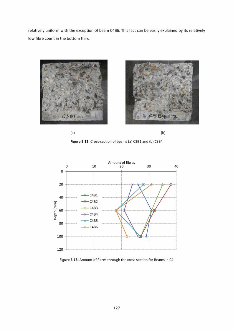
127
relatively uniform with the exception of beam C4B6. This fact can be easily explained by its relatively
low fibre count in the bottom third.
(a) (b)
Figure 5.12: Cross-section of beams (a) C3B1 and (b) C3B4
Figure 5.13: Amount of fibres through the cross section for Beams in C4
0
20
40
60
80
100
120
0 10 20 30 40
Dep
th (
mm
)
Amount of fibres
C4B1
C4B2
C4B3
C4B4
C4B5
C4B6
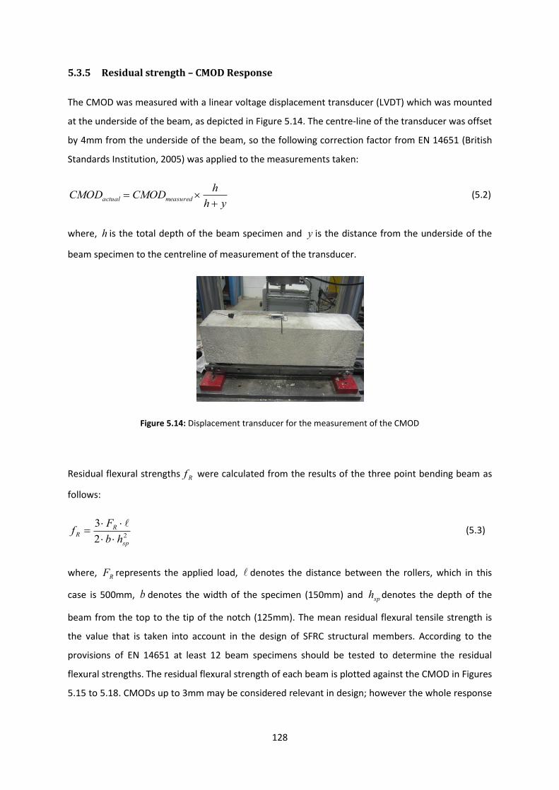
128
5.3.5 Residual strength – CMOD Response
The CMOD was measured with a linear voltage displacement transducer (LVDT) which was mounted
at the underside of the beam, as depicted in Figure 5.14. The centre-line of the transducer was offset
by 4mm from the underside of the beam, so the following correction factor from EN 14651 (British
Standards Institution, 2005) was applied to the measurements taken:
yh
hCMODCMOD measuredactual
(5.2)
where, h is the total depth of the beam specimen and y is the distance from the underside of the
beam specimen to the centreline of measurement of the transducer.
Figure 5.14: Displacement transducer for the measurement of the CMOD
Residual flexural strengths Rf were calculated from the results of the three point bending beam as
follows:
22
3
sp
RR
hb
Ff
(5.3)
where, RF represents the applied load, denotes the distance between the rollers, which in this
case is 500mm, b denotes the width of the specimen (150mm) and sph denotes the depth of the
beam from the top to the tip of the notch (125mm). The mean residual flexural tensile strength is
the value that is taken into account in the design of SFRC structural members. According to the
provisions of EN 14651 at least 12 beam specimens should be tested to determine the residual
flexural strengths. The residual flexural strength of each beam is plotted against the CMOD in Figures
5.15 to 5.18. CMODs up to 3mm may be considered relevant in design; however the whole response
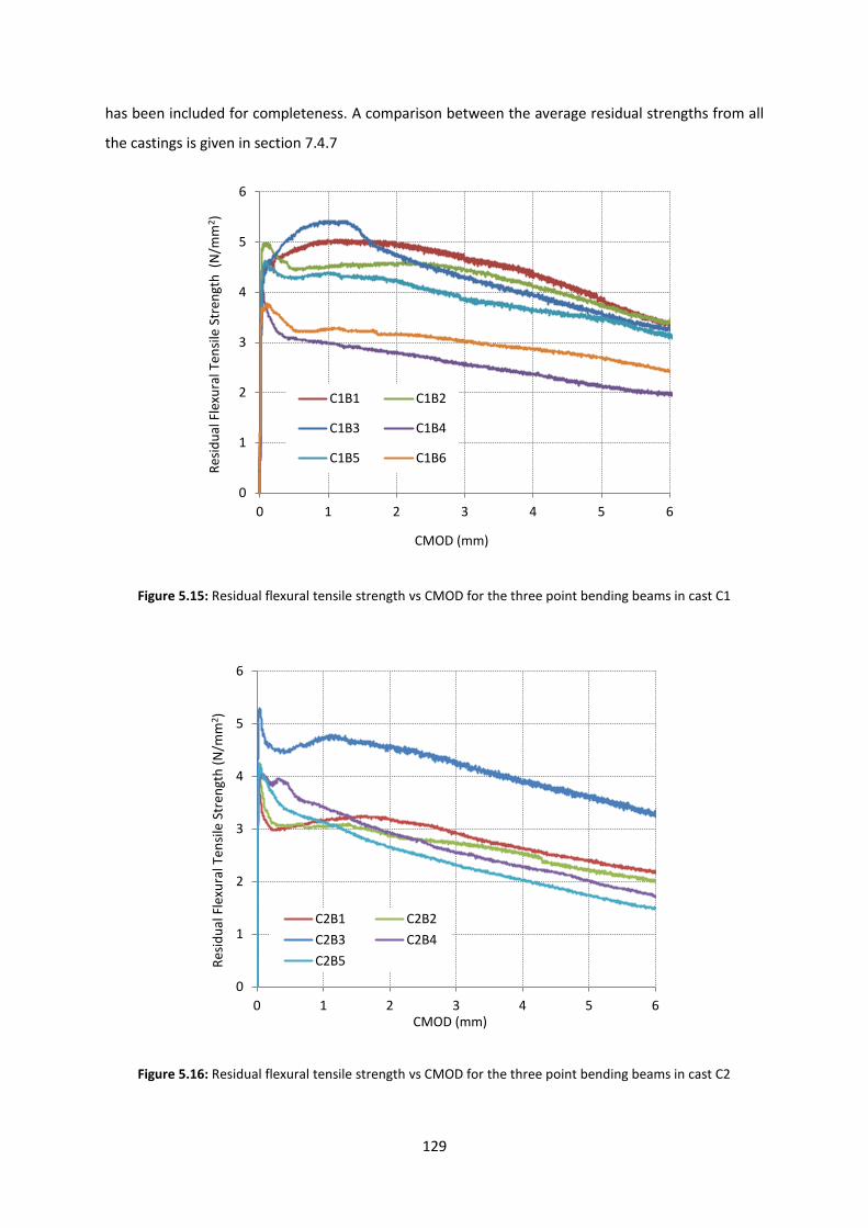
129
has been included for completeness. A comparison between the average residual strengths from all
the castings is given in section 7.4.7
Figure 5.15: Residual flexural tensile strength vs CMOD for the three point bending beams in cast C1
Figure 5.16: Residual flexural tensile strength vs CMOD for the three point bending beams in cast C2
0
1
2
3
4
5
6
0 1 2 3 4 5 6
Res
idu
al F
lexu
ral T
ensi
le S
tren
gth
(N
/mm
2 )
CMOD (mm)
C1B1 C1B2
C1B3 C1B4
C1B5 C1B6
0
1
2
3
4
5
6
0 1 2 3 4 5 6
Res
idu
al F
lexu
ral T
ensi
le S
tren
gth
(N
/mm
2)
CMOD (mm)
C2B1 C2B2
C2B3 C2B4
C2B5

130
Figure 5.17: Residual flexural tensile strength vs CMOD for the three point bending beams in cast C3
Figure 5.18: Residual flexural tensile strength vs CMOD for the three point bending beams in cast C4
0
1
2
3
4
5
6
0 1 2 3 4 5 6
Res
idu
al F
lexu
ral T
ensi
le S
tren
gth
(N
/mm
2)
CMOD (mm)
C3B1 C3B2
C3B3 C3B4
C3B5 C3B6
0
1
2
3
4
5
6
0 1 2 3 4 5 6
Res
idu
al F
lexu
ral T
ensi
le S
tren
gth
(N
/mm
2)
CMOD (mm)
C4B1 C4B2
C4B3 C4B4
C4B5
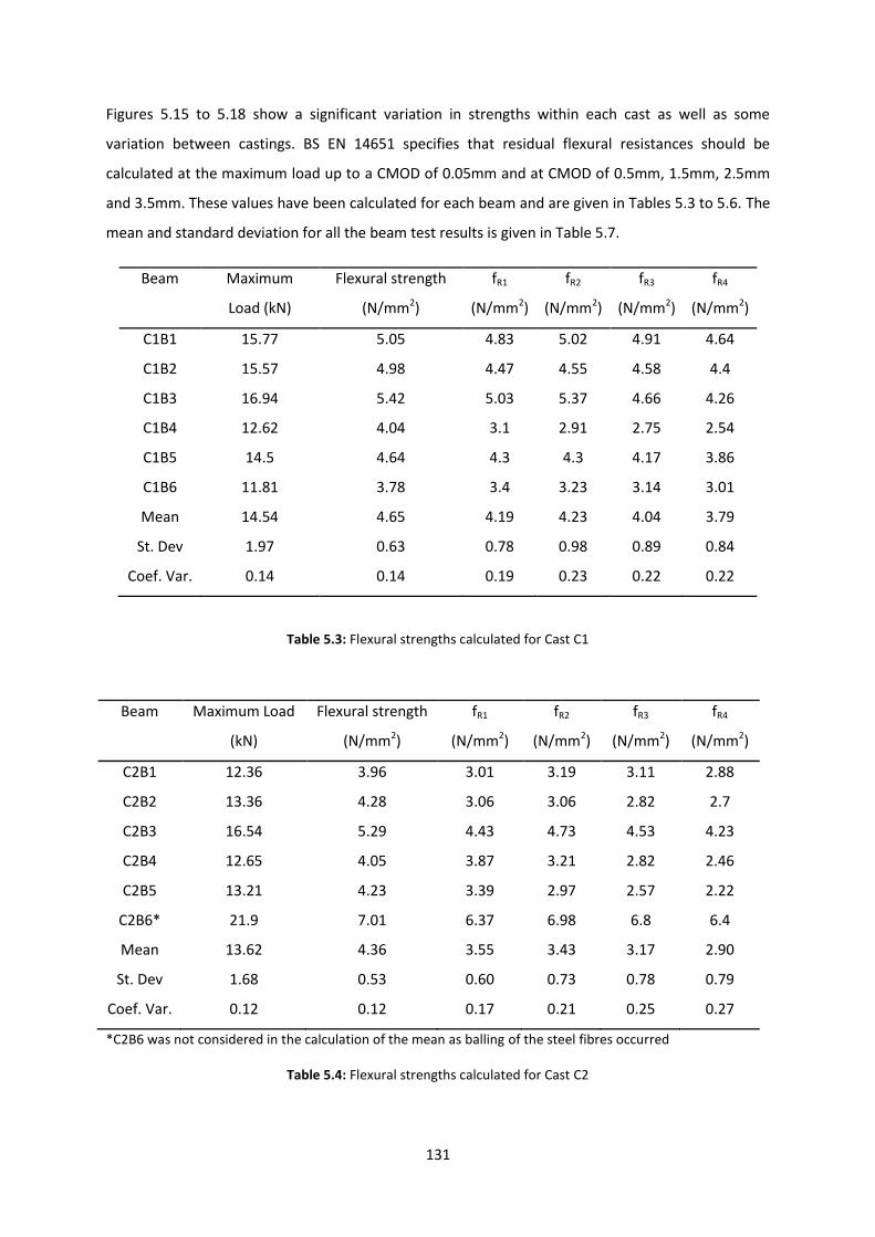
131
Figures 5.15 to 5.18 show a significant variation in strengths within each cast as well as some
variation between castings. BS EN 14651 specifies that residual flexural resistances should be
calculated at the maximum load up to a CMOD of 0.05mm and at CMOD of 0.5mm, 1.5mm, 2.5mm
and 3.5mm. These values have been calculated for each beam and are given in Tables 5.3 to 5.6. The
mean and standard deviation for all the beam test results is given in Table 5.7.
Beam Maximum
Load (kN)
Flexural strength
(N/mm2)
fR1
(N/mm2)
fR2
(N/mm2)
fR3
(N/mm2)
fR4
(N/mm2)
C1B1 15.77 5.05 4.83 5.02 4.91 4.64
C1B2 15.57 4.98 4.47 4.55 4.58 4.4
C1B3 16.94 5.42 5.03 5.37 4.66 4.26
C1B4 12.62 4.04 3.1 2.91 2.75 2.54
C1B5 14.5 4.64 4.3 4.3 4.17 3.86
C1B6 11.81 3.78 3.4 3.23 3.14 3.01
Mean 14.54 4.65 4.19 4.23 4.04 3.79
St. Dev 1.97 0.63 0.78 0.98 0.89 0.84
Coef. Var. 0.14 0.14 0.19 0.23 0.22 0.22
Table 5.3: Flexural strengths calculated for Cast C1
Beam Maximum Load
(kN)
Flexural strength
(N/mm2)
fR1
(N/mm2)
fR2
(N/mm2)
fR3
(N/mm2)
fR4
(N/mm2)
C2B1 12.36 3.96 3.01 3.19 3.11 2.88
C2B2 13.36 4.28 3.06 3.06 2.82 2.7
C2B3 16.54 5.29 4.43 4.73 4.53 4.23
C2B4 12.65 4.05 3.87 3.21 2.82 2.46
C2B5 13.21 4.23 3.39 2.97 2.57 2.22
C2B6* 21.9 7.01 6.37 6.98 6.8 6.4
Mean 13.62 4.36 3.55 3.43 3.17 2.90
St. Dev 1.68 0.53 0.60 0.73 0.78 0.79
Coef. Var. 0.12 0.12 0.17 0.21 0.25 0.27
*C2B6 was not considered in the calculation of the mean as balling of the steel fibres occurred
Table 5.4: Flexural strengths calculated for Cast C2

132
Beam Maximum
Load (kN)
Flexural strength
(N/mm2)
fR1
(N/mm2)
fR2
(N/mm2)
fR3
(N/mm2)
fR4
(N/mm2)
C3B1 15.52 4.97 4.85 4.93 4.78 4.52
C3B2 16.48 5.27 5.09 4.92 5.12 4.71
C3B3 13.75 4.4 3.82 3.82 3.67 3.45
C3B4 12.82 4.1 3.8 3.87 3.78 3.58
C3B5 13.16 4.21 3.84 3.69 3.44 3.16
C3B6 15.16 4.85 3.9 3.92 3.93 3.82
Mean 14.48 4.63 4.22 4.19 4.12 3.87
St. Dev 1.45 0.47 0.59 0.57 0.67 0.62
Coef. Var. 0.10 0.10 0.14 0.14 0.16 0.16
Table 5.5: Flexural strengths calculated for Cast C3
Beam Maximum
Load (kN)
Flexural strength
(N/mm2)
fR1
(N/mm2)
fR2
(N/mm2)
fR3
(N/mm2)
fR4
(N/mm2)
C4B1 15.93 5.1 4.64 4.59 4.46 5.1
C4B2 13.63 4.36 4.09 4.24 4.15 3.87
C4B3 13.39 4.28 4.2 4.19 3.95 3.76
C4B4 13.72 4.39 4.01 3.97 3.74 3.38
C4B5 14.82 4.74 4.68 4.36 3.61 3.19
C4B6 11.1 3.55 2.82 2.38 2.08 1.9
Mean 13.77 4.40 4.07 3.96 3.67 3.53
St. Dev 1.62 0.52 0.68 0.80 0.83 1.04
Coef. Var. 0.12 0.12 0.17 0.20 0.23 0.29
Table 5.6: Flexural strengths calculated for Cast C4
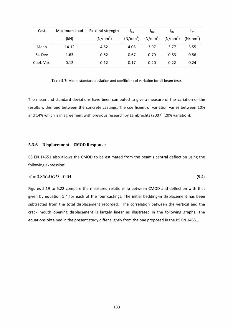
133
Cast Maximum Load
(kN)
Flexural strength
(N/mm2)
fR1
(N/mm2)
fR2
(N/mm2)
fR3
(N/mm2)
fR4
(N/mm2)
Mean 14.12 4.52 4.03 3.97 3.77 3.55
St. Dev 1.63 0.52 0.67 0.79 0.83 0.86
Coef. Var. 0.12 0.12 0.17 0.20 0.22 0.24
Table 5.7: Mean, standard deviation and coefficient of variation for all beam tests
The mean and standard deviations have been computed to give a measure of the variation of the
results within and between the concrete castings. The coefficient of variation varies between 10%
and 14% which is in agreement with previous research by Lambrechts (2007) (20% variation).
5.3.6 Displacement – CMOD Response
BS EN 14651 also allows the CMOD to be estimated from the beam’s central deflection using the
following expression:
04.085.0 CMOD (5.4)
Figures 5.19 to 5.22 compare the measured relationship between CMOD and deflection with that
given by equation 5.4 for each of the four castings. The initial bedding-in displacement has been
subtracted from the total displacement recorded. The correlation between the vertical and the
crack mouth opening displacement is largely linear as illustrated in the following graphs. The
equations obtained in the present study differ slightly from the one proposed in the BS EN 14651.

134
Figure 5.19: Three point bending CMOD – Vertical Displacement response for Cast 1
Figure 5.20: Three point bending CMOD – Vertical Displacement response for Cast 2
y = 0.9074x + 0.0727
0
2
4
6
8
0 1 2 3 4 5 6
Dis
pla
cem
ent
(mm
)
CMOD (mm)
C1B1 C1B2
C1B3 C1B4
C1B5 C1B6
EN 14651 Linear (C1B1)
y = 0.8972x + 0.0395
0
2
4
6
8
0 1 2 3 4 5 6
Dis
pla
cem
ent
(mm
)
CMOD (mm)
C2B1
C2B2
C2B3
C2B4
C2B5
C2B6
EN 14651
Linear (C2B1)
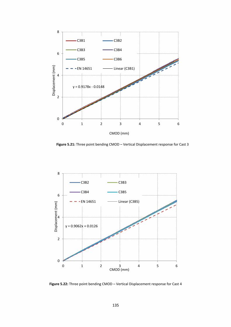
135
Figure 5.21: Three point bending CMOD – Vertical Displacement response for Cast 3
Figure 5.22: Three point bending CMOD – Vertical Displacement response for Cast 4
y = 0.9178x - 0.0148
0
2
4
6
8
0 1 2 3 4 5 6
Dis
pla
cem
ent
(mm
)
CMOD (mm)
C3B1 C3B2
C3B3 C3B4
C3B5 C3B6
EN 14651 Linear (C3B1)
y = 0.9062x + 0.0126
0
2
4
6
8
0 1 2 3 4 5 6
Dis
pla
cem
ent
(mm
)
CMOD (mm)
C3B2 C3B3
C3B4 C3B5
EN 14651 Linear (C3B5)

136
5.4 Statically Determinate Round Plate Tests
5.4.1 General Overview
This section gives the results of the tests on the Round Determinate Plate Tests. The test procedure
as well as the instrumentation adopted is described in Section 4.5 of the thesis. Although less
straight-forward, such tests would appear to simulate the behaviour of SFRC pile-supported slabs
more accurately than the three-point bending beams as the results are less sensitive to random
variations in the fibre distribution due to the greater area of the crack surfaces (Lambrechts A. N.,
2007).
5.4.2 Results
Statically determinate round plates tend to fail by the formation of three even cracks, as shown in
Figure 5.23. Figure 5.24 shows the load displacement response measured in the three RDP tests
from Cast 1.
(a)
(b)
Figure 5.23: Typical failure mechanism of a statically determinate round panel specimen
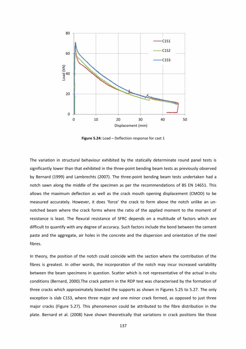
137
Figure 5.24: Load – Deflection response for cast 1
The variation in structural behaviour exhibited by the statically determinate round panel tests is
significantly lower than that exhibited in the three-point bending beam tests as previously observed
by Bernard (1999) and Lambrechts (2007). The three-point bending beam tests undertaken had a
notch sawn along the middle of the specimen as per the recommendations of BS EN 14651. This
allows the maximum deflection as well as the crack mouth opening displacement (CMOD) to be
measured accurately. However, it does ‘force’ the crack to form above the notch unlike an un-
notched beam where the crack forms where the ratio of the applied moment to the moment of
resistance is least. The flexural resistance of SFRC depends on a multitude of factors which are
difficult to quantify with any degree of accuracy. Such factors include the bond between the cement
paste and the aggregate, air holes in the concrete and the dispersion and orientation of the steel
fibres.
In theory, the position of the notch could coincide with the section where the contribution of the
fibres is greatest. In other words, the incorporation of the notch may incur increased variability
between the beam specimens in question. Scatter which is not representative of the actual in-situ
conditions (Bernard, 2000).The crack pattern in the RDP test was characterised by the formation of
three cracks which approximately bisected the supports as shown in Figures 5.25 to 5.27. The only
exception is slab C1S3, where three major and one minor crack formed, as opposed to just three
major cracks (Figure 5.27). This phenomenon could be attributed to the fibre distribution in the
plate. Bernard et al. (2008) have shown theoretically that variations in crack positions like those
0
20
40
60
80
0 10 20 30 40 50
Load
(kN
)
Displacement (mm)
C1S1
C1S2
C1S3

138
shown in Figure 5.27 do not significantly affect the load displacement of the RDP. This was also
confirmed experimentally by comparing the load displacements responses of slabs C1S1 and C1S2
with those of slab C1S3 (Figure 5.24).
(a)
(b)
Figure 5.25: Crack pattern for slab C1S1 (a) photograph (b) angles at which the cracks form

139
(a)
(b)
Figure 5.26: Crack pattern for slab C1S2 (a) photograph (b) angles at which the cracks form
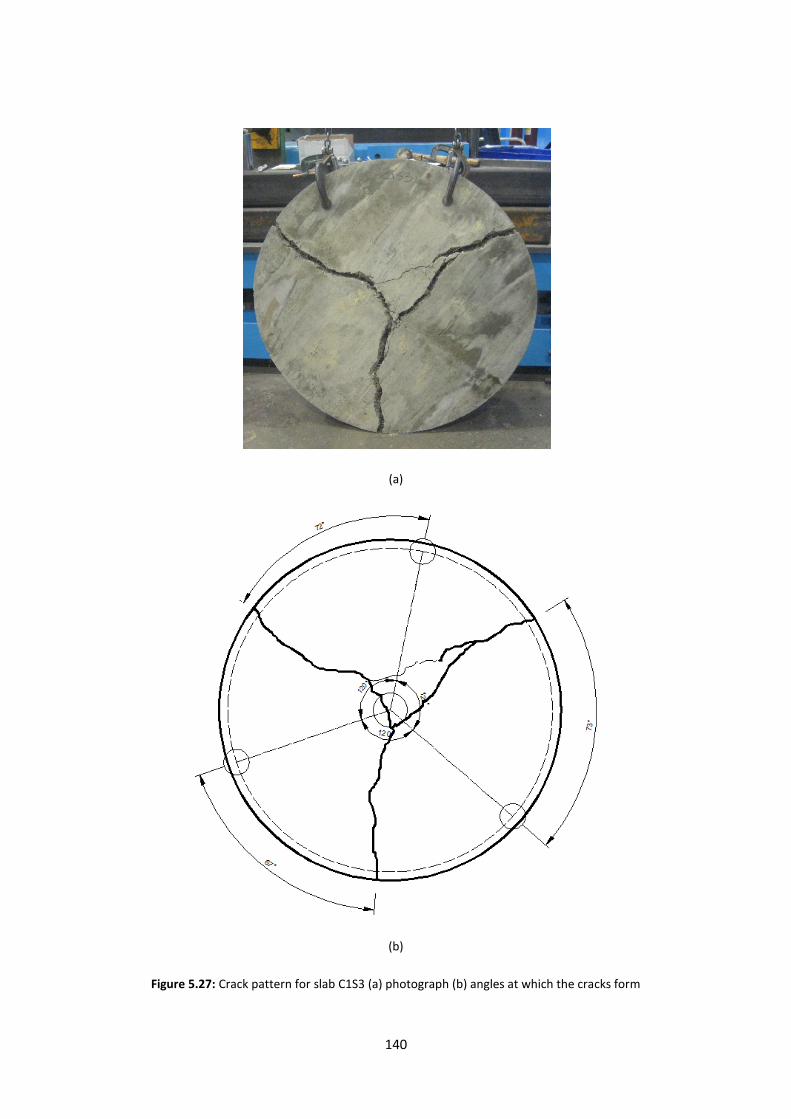
140
(a)
(b)
Figure 5.27: Crack pattern for slab C1S3 (a) photograph (b) angles at which the cracks form
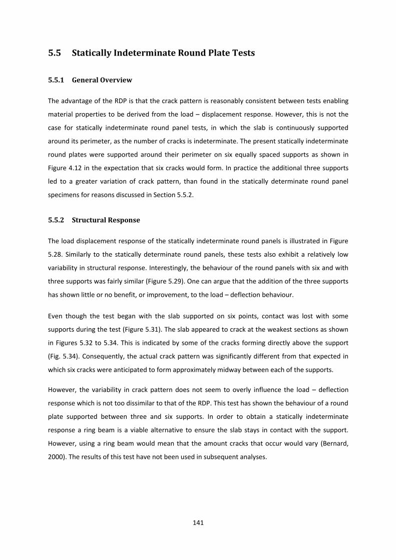
141
5.5 Statically Indeterminate Round Plate Tests
5.5.1 General Overview
The advantage of the RDP is that the crack pattern is reasonably consistent between tests enabling
material properties to be derived from the load – displacement response. However, this is not the
case for statically indeterminate round panel tests, in which the slab is continuously supported
around its perimeter, as the number of cracks is indeterminate. The present statically indeterminate
round plates were supported around their perimeter on six equally spaced supports as shown in
Figure 4.12 in the expectation that six cracks would form. In practice the additional three supports
led to a greater variation of crack pattern, than found in the statically determinate round panel
specimens for reasons discussed in Section 5.5.2.
5.5.2 Structural Response
The load displacement response of the statically indeterminate round panels is illustrated in Figure
5.28. Similarly to the statically determinate round panels, these tests also exhibit a relatively low
variability in structural response. Interestingly, the behaviour of the round panels with six and with
three supports was fairly similar (Figure 5.29). One can argue that the addition of the three supports
has shown little or no benefit, or improvement, to the load – deflection behaviour.
Even though the test began with the slab supported on six points, contact was lost with some
supports during the test (Figure 5.31). The slab appeared to crack at the weakest sections as shown
in Figures 5.32 to 5.34. This is indicated by some of the cracks forming directly above the support
(Fig. 5.34). Consequently, the actual crack pattern was significantly different from that expected in
which six cracks were anticipated to form approximately midway between each of the supports.
However, the variability in crack pattern does not seem to overly influence the load – deflection
response which is not too dissimilar to that of the RDP. This test has shown the behaviour of a round
plate supported between three and six supports. In order to obtain a statically indeterminate
response a ring beam is a viable alternative to ensure the slab stays in contact with the support.
However, using a ring beam would mean that the amount cracks that occur would vary (Bernard,
2000). The results of this test have not been used in subsequent analyses.
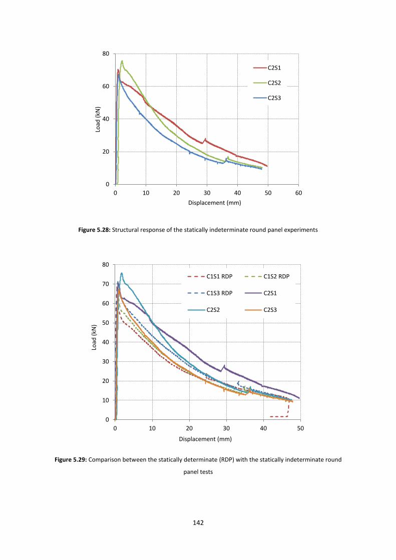
142
Figure 5.28: Structural response of the statically indeterminate round panel experiments
Figure 5.29: Comparison between the statically determinate (RDP) with the statically indeterminate round
panel tests
0
20
40
60
80
0 10 20 30 40 50 60
Load
(kN
)
Displacement (mm)
C2S1
C2S2
C2S3
0
10
20
30
40
50
60
70
80
0 10 20 30 40 50
Load
(kN
)
Displacement (mm)
C1S1 RDP C1S2 RDP
C1S3 RDP C2S1
C2S2 C2S3
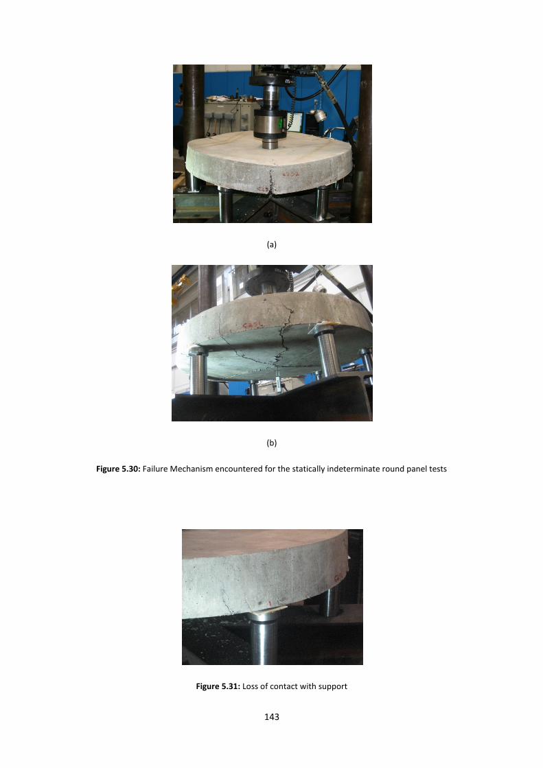
143
(a)
(b)
Figure 5.30: Failure Mechanism encountered for the statically indeterminate round panel tests
Figure 5.31: Loss of contact with support
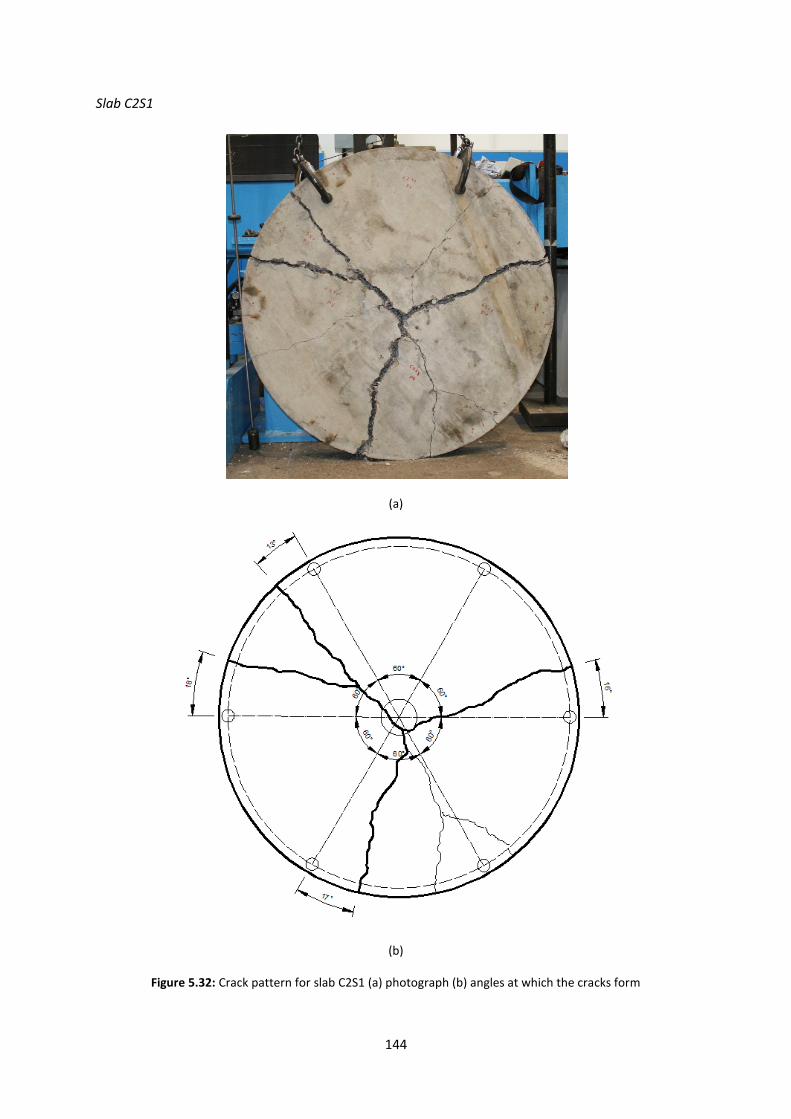
144
Slab C2S1
(a)
(b)
Figure 5.32: Crack pattern for slab C2S1 (a) photograph (b) angles at which the cracks form
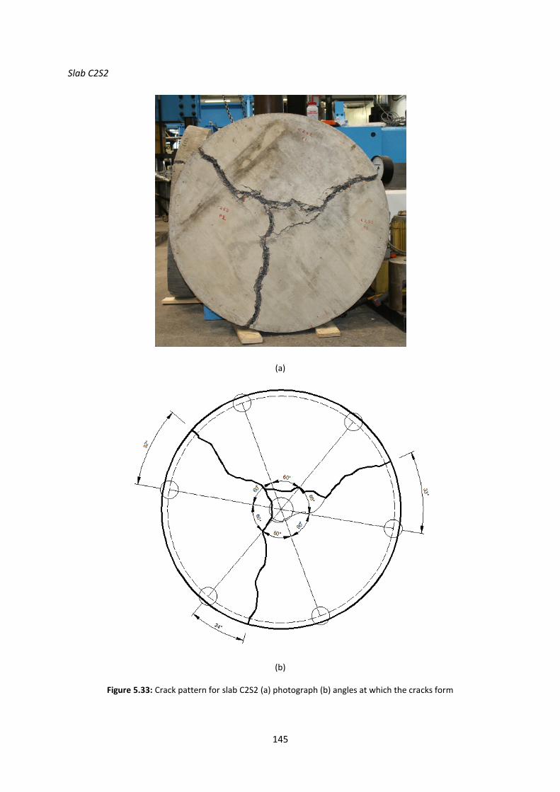
145
Slab C2S2
(a)
(b)
Figure 5.33: Crack pattern for slab C2S2 (a) photograph (b) angles at which the cracks form

146
Slab C2S3
(a)
(b)
Figure 5.34: Crack pattern for slab C2S3 (a) photograph (b) angles at which the cracks form
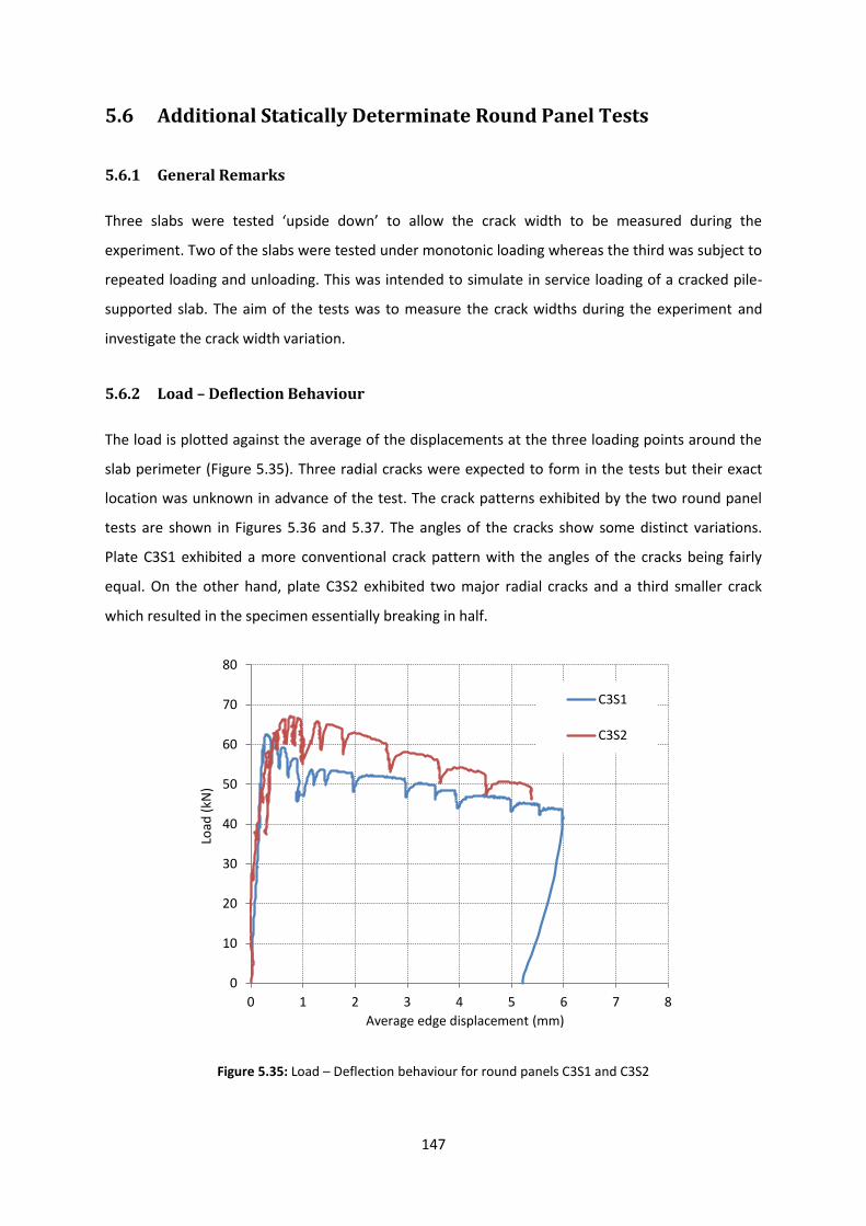
147
5.6 Additional Statically Determinate Round Panel Tests
5.6.1 General Remarks
Three slabs were tested ‘upside down’ to allow the crack width to be measured during the
experiment. Two of the slabs were tested under monotonic loading whereas the third was subject to
repeated loading and unloading. This was intended to simulate in service loading of a cracked pile-
supported slab. The aim of the tests was to measure the crack widths during the experiment and
investigate the crack width variation.
5.6.2 Load – Deflection Behaviour
The load is plotted against the average of the displacements at the three loading points around the
slab perimeter (Figure 5.35). Three radial cracks were expected to form in the tests but their exact
location was unknown in advance of the test. The crack patterns exhibited by the two round panel
tests are shown in Figures 5.36 and 5.37. The angles of the cracks show some distinct variations.
Plate C3S1 exhibited a more conventional crack pattern with the angles of the cracks being fairly
equal. On the other hand, plate C3S2 exhibited two major radial cracks and a third smaller crack
which resulted in the specimen essentially breaking in half.
Figure 5.35: Load – Deflection behaviour for round panels C3S1 and C3S2
0
10
20
30
40
50
60
70
80
0 1 2 3 4 5 6 7 8
Load
(kN
)
Average edge displacement (mm)
C3S1
C3S2

148
(a)
(b)
Figure 5.36: Crack pattern for slab C3S1 (a) photograph (b) angles at which the cracks form
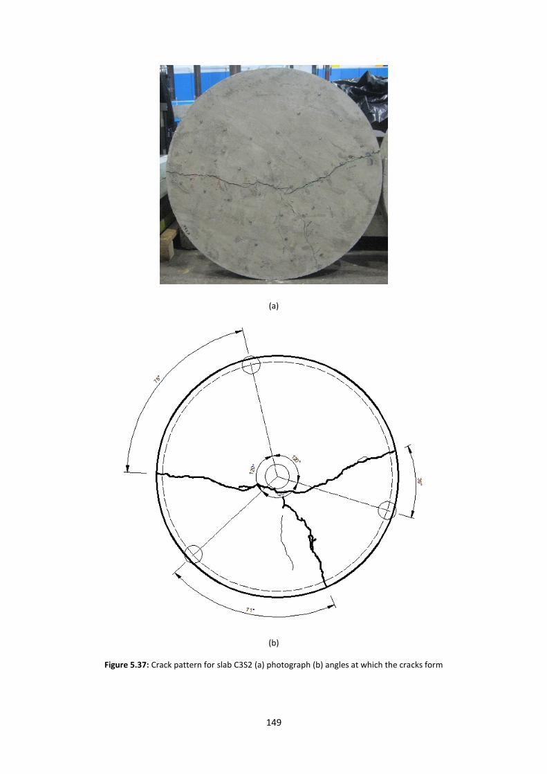
149
(a)
(b)
Figure 5.37: Crack pattern for slab C3S2 (a) photograph (b) angles at which the cracks form

150
5.6.3 Crack Widths
Round SFRC plates have been tested by many researchers (Barros & Figueiras, 2001) (Bernard, 2000)
(Bernard & Pircher, 2000) (Sukontasukkul, 2003) (Soranakom, 2008) (Bernard, 2008) (Arcelor, 2010
TBR) but as far as the author is aware none of these researchers have made direct measurements of
crack widths in round plate tests. This is no doubt a consequence of the round plate being
conventionally loaded from the top. At the time of writing, there are no recommendations or
provisions in any of the codes for the calculation of crack width in SFRC slabs without conventional
reinforcement. The experimental setup was designed, as mentioned in Chapter Four, with the aim of
directly measuring crack widths. The results obtained regarding the cracking behaviour of the SFRC
are presented in the sub-sections that follow. The locations of the Demec points and the transducers
in relation to the cracks formed are shown in Figure 5.38 and 5.39 for slabs C3S1 and C3S2
respectively.
Crack widths were estimated from the Demec strain measurements as the product of the gauge
length (150mm) and the difference between the total and elastic strains. The elastic strain was
assumed to equal the assumed cracking strain of 100μs at the peak load. Subsequently, it was
assumed to reduce linearly in proportion with the applied load as follows:
crcrP
P
max
mod (5.5)
where, P is the applied load, maxP is the peak load and cr is the cracking strain.
The error in crack width associated with this approximation is small since the peak elastic extension
over the 150mm gauge length is only 0.015mm which is typically at least an order of magnitude less
than the measured crack widths.
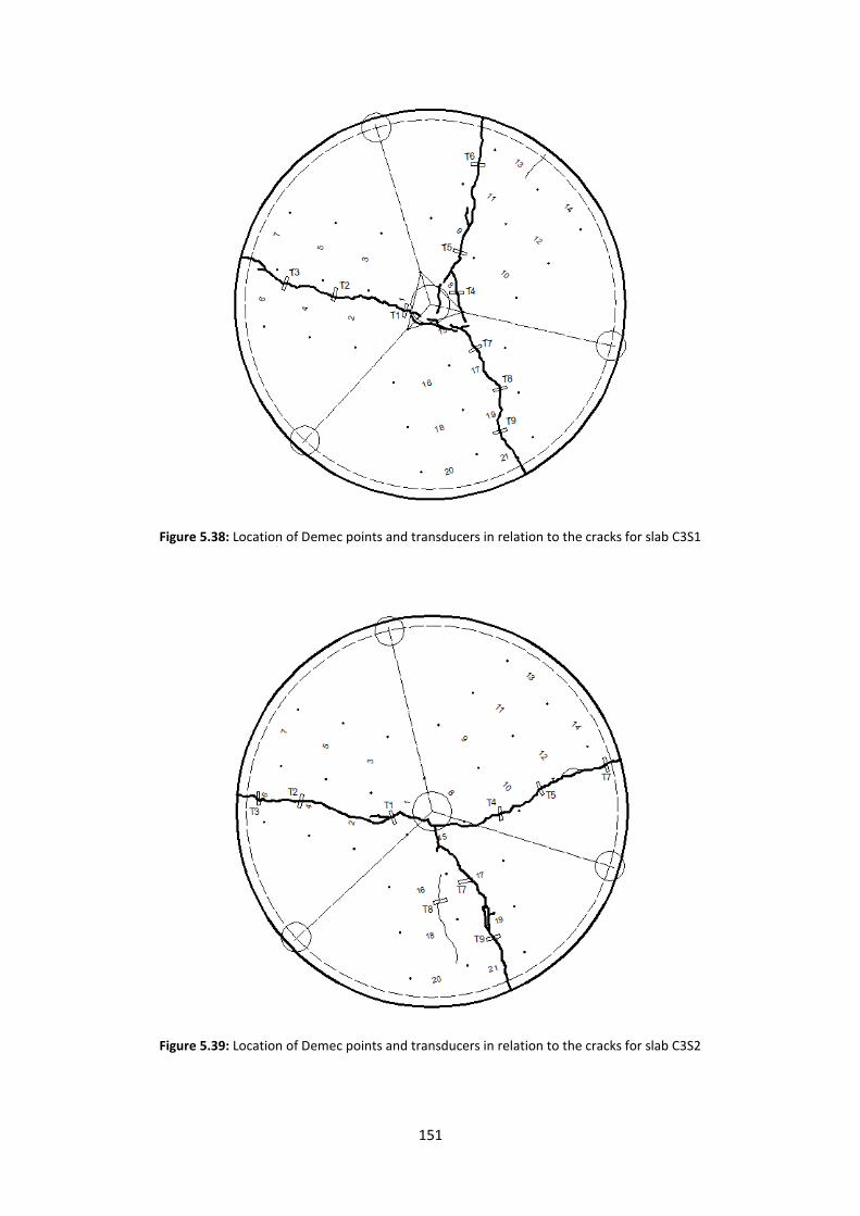
151
Figure 5.38: Location of Demec points and transducers in relation to the cracks for slab C3S1
Figure 5.39: Location of Demec points and transducers in relation to the cracks for slab C3S2

152
Figure 5.40: Crack width measurements in crack 3 (Slab C3S1)
For each distinct crack that was formed, the crack width response was recorded with the already
mounted Demec points as well as transducers which were mounted once the cracks had formed
(Figure 5.40). The transducers were mounted as close as possible to the Demec points in order to
have some overlap in readings to confirm the validity of the results. The crack width is plotted
against the average edge displacement in Figures 5.41 to 5.48, which should be read in conjunction
with Figures 5.38 and 5.39 which define the position of the Demec points and the transducers for
slabs C3S1 and C3S2. The ‘overlapping’ results between the Demec points and the transducers seem
to show a reasonably good agreement.
Figures 5.41 to 5.43 indicate that slab C3S1 cracked at a central displacement of approximately
1.4mm. After cracking the displacement – crack width is characterised by a linear response. The
behaviour of cracks two and three is very similar, particularly for crack widths less than 1.5mm.
However, both of these exhibit significant differences compared to the behaviour of crack one.
Unlike slab C3S1, a less uniform crack pattern developed in C3S2. There are two main cracks that
have effectively formed approximately 180 degrees from each other. This would seem to suggest
that the sections where the cracks formed were considerably weaker than elsewhere, especially
considering the fact that one of the cracks formed rather close to one of the supports.
In Figures 5.46 and 5.47 the relationship between crack opening and displacement is very similar for
all three cracks. Figure 5.48 seems consistent with the observation that the slab effectively broke
into two rather than three segments. Cracks one and two have similar widths, whereas crack three is
considerably narrower. Despite the significant difference in crack pattern, the load displacement
responses of slabs C3S1 and C3S2 are similar.
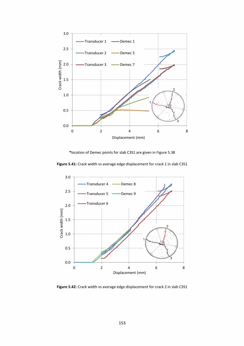
153
*location of Demec points for slab C3S1 are given in Figure 5.38
Figure 5.41: Crack width vs average edge displacement for crack 1 in slab C3S1
Figure 5.42: Crack width vs average edge displacement for crack 2 in slab C3S1
0.0
0.5
1.0
1.5
2.0
2.5
3.0
0 2 4 6 8
Cra
ck w
idth
(m
m)
Displacement (mm)
Transducer 1 Demec 1
Transducer 2 Demec 5
Transducer 3 Demec 7
0.0
0.5
1.0
1.5
2.0
2.5
3.0
0 2 4 6 8
Cra
ck w
idth
(m
m)
Displacement (mm)
Transducer 4 Demec 8
Transducer 5 Demec 9
Transducer 6

154
Figure 5.43: Crack width vs average edge displacement for crack 3 in C3S1
Figure 5.44: Displacement vs crack width comparison between the three cracks formed in slab C3S1
0
1
2
3
4
5
0 2 4 6 8
Cra
ck w
idth
(m
m)
Displacement (mm)
Demec 19 Transducer 8
Transducer 9 Demec 17
Demec 21 Transducer 7
Demec 15
0
1
2
3
4
5
0 2 4 6 8
Cra
ck w
idth
(m
m)
Displacement (mm)
Crack 1 - Transducer 1
Crack 1 - Demec 1
Crack 2 - Transducer 4
Crack 2 - Demec 7
Crack 3 - Demec 17
Crack 3 - Transducer 7
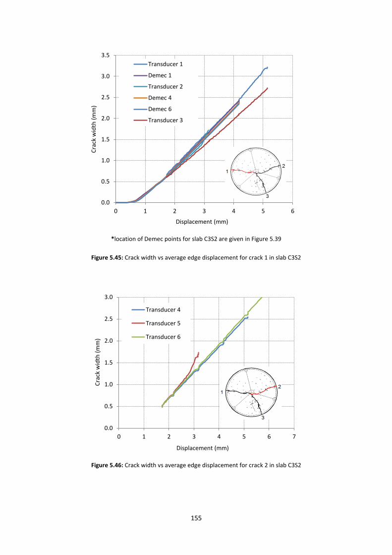
155
*location of Demec points for slab C3S2 are given in Figure 5.39
Figure 5.45: Crack width vs average edge displacement for crack 1 in slab C3S2
Figure 5.46: Crack width vs average edge displacement for crack 2 in slab C3S2
0.0
0.5
1.0
1.5
2.0
2.5
3.0
3.5
0 1 2 3 4 5 6
Cra
ck w
idth
(m
m)
Displacement (mm)
Transducer 1
Demec 1
Transducer 2
Demec 4
Demec 6
Transducer 3
0.0
0.5
1.0
1.5
2.0
2.5
3.0
0 1 2 3 4 5 6 7
Cra
ck w
idth
(m
m)
Displacement (mm)
Transducer 4
Transducer 5
Transducer 6

156
Figure 5.47: Crack width vs average edge displacement for crack 3 in slab C3S2
Figure 5.48: Displacement vs crack width comparison between the three cracks formed in slab C3S2
0.0
0.3
0.5
0.8
1.0
1.3
1.5
1.8
2.0
0 1 2 3 4 5 6 7 8
Cra
ck w
idth
(m
m)
Displacement (mm)
Transducer 7 Transducer 9
Demec 15 Demec 19
Demec 21 Demec 17
0.0
0.5
1.0
1.5
2.0
2.5
3.0
3.5
0 1 2 3 4 5 6 7 8
Cra
ck w
idth
(m
m)
Displacement (mm)
Crack 3 - Transducer 7
Crack 3 - Demec 19
Crack 2 - Transducer 6
Crack 1 - Transducer 1
Crack 1 - Demec 1
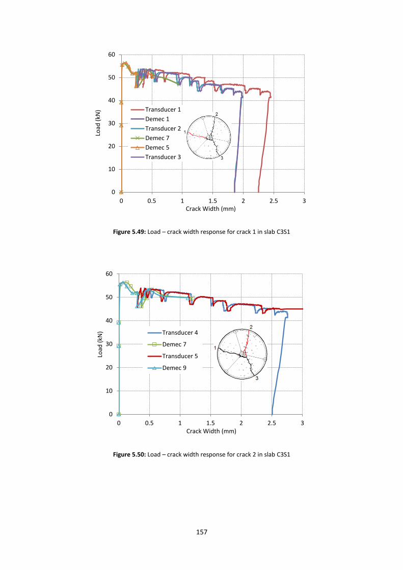
157
Figure 5.49: Load – crack width response for crack 1 in slab C3S1
Figure 5.50: Load – crack width response for crack 2 in slab C3S1
0
10
20
30
40
50
60
0 0.5 1 1.5 2 2.5 3
Load
(kN
)
Crack Width (mm)
Transducer 1
Demec 1
Transducer 2
Demec 7
Demec 5
Transducer 3
0
10
20
30
40
50
60
0 0.5 1 1.5 2 2.5 3
Load
(kN
)
Crack Width (mm)
Transducer 4
Demec 7
Transducer 5
Demec 9

158
Figure 5.51: Load – crack width response for crack 3 in slab C3S1
Figure 5.52: Load – crack width response for crack 1 in slab C3S2
0
10
20
30
40
50
60
0 0.5 1 1.5 2 2.5 3 3.5 4
Load
(kN
)
Crack Width(mm)
Transducer 8
Transducer 9
Demec 21
Transducer 7
Demec 15
0
10
20
30
40
50
60
70
0 0.5 1 1.5 2 2.5 3 3.5 4
Load
(kN
)
Crack width (mm)
Transducer 1
Transducer 2
Demec 5
Demec 6
Transducer 3

159
Figure 5.53: Load – crack width response for crack 2 in slab C3S2
Figure 5.54: Load – crack width response for crack 3 in slab C3S2
0
10
20
30
40
50
60
70
0 0.5 1 1.5 2 2.5 3 3.5 4
Load
(kN
)
Crack width (mm)
Transducer 4
Transducer 5
Transducer 6
0
10
20
30
40
50
60
70
0 0.25 0.5 0.75 1 1.25 1.5 1.75
Load
(kN
)
Crack width (mm)
Transducer 7
Transducer 9
Demec 19
Demec 17

160
5.6.4 Crack Width along a Fracture Surface
The yield line method is commonly used for the design of SFRC pile-supported slabs. A number of
assumptions are made in the method as discussed in Chapter Three. One of the key assumptions is
that the moment is constant along a crack which in turn implies that the crack width is uniform along
its length. In traditional reinforced concrete structures such a simplification may be regarded as
acceptable given that the structural member in question exhibits a tension hardening response.
This assumption is investigated by plotting the crack width along each crack at various displacements
in Figures 5.55 to 5.60 for slabs C3S1 and C3S2. The crack widths have been plotted using the output
of the Demec points.
Figures 5.55 to 5.60 show that there is some variation in crack width along its length particularly for
crack widths below approximately 0.7mm. However, the data are inconsistent and in some cases the
crack width appears to be virtually constant along its length. Where there is a variation in crack
width, the width is typically greatest at the centre of the plate and reduces with increasing distance
from the centre as shown in Figure 5.55.
Slab C3S1
* crack widths plotted using the results of the Demec points at various displacements
Figure 5.55: Crack width at various displacements – Slab C3S1 – Crack 1
0.0
0.1
0.2
0.3
0.4
0.5
0.6
0.7
0.8
0 100 200 300 400
Cra
ck W
idth
(m
m)
Distance from centre (mm)
2.60mm
2.20mm
1.87mm
1.57mm
1.37mm
1.20mm
1.05mm
0.90mm

161
Figure 5.56: Crack width at various displacements – Slab C3S1 – Crack 2
Figure 5.57: Crack width at various displacements – Slab C3S1 – Crack 3
0.0
0.1
0.2
0.3
0.4
0.5
0.6
0.7
0.8
0 100 200 300 400
Cra
ck W
idth
(m
m)
Distance from centre (mm)
2.61mm
2.20mm
1.87mm
1.57mm
1.37mm
1.20mm
1.05mm
0.90mm
0.0
0.2
0.4
0.6
0.8
1.0
1.2
1.4
0 100 200 300 400 500
Cra
ck W
idth
(m
m)
Distance from centre (mm)
2.61mm
2.20mm
1.87mm
1.57mm
1.37mm
1.20mm
1.05mm
0.90mm
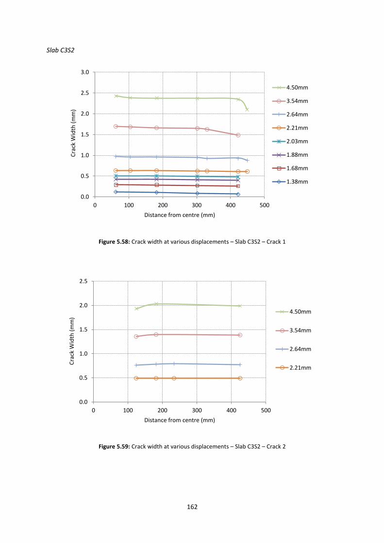
162
Slab C3S2
Figure 5.58: Crack width at various displacements – Slab C3S2 – Crack 1
Figure 5.59: Crack width at various displacements – Slab C3S2 – Crack 2
0.0
0.5
1.0
1.5
2.0
2.5
3.0
0 100 200 300 400 500
Cra
ck W
idth
(m
m)
Distance from centre (mm)
4.50mm
3.54mm
2.64mm
2.21mm
2.03mm
1.88mm
1.68mm
1.38mm
0.0
0.5
1.0
1.5
2.0
2.5
0 100 200 300 400 500
Cra
ck W
idth
(m
m)
Distance from centre (mm)
4.50mm
3.54mm
2.64mm
2.21mm
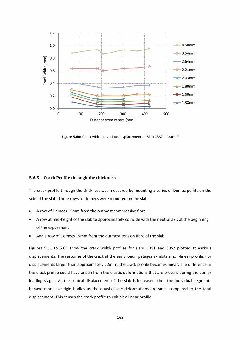
163
Figure 5.60: Crack width at various displacements – Slab C3S2 – Crack 2
5.6.5 Crack Profile through the thickness
The crack profile through the thickness was measured by mounting a series of Demec points on the
side of the slab. Three rows of Demecs were mounted on the slab:
A row of Demecs 15mm from the outmost compressive fibre
A row at mid-height of the slab to approximately coincide with the neutral axis at the beginning
of the experiment
And a row of Demecs 15mm from the outmost tension fibre of the slab
Figures 5.61 to 5.64 show the crack width profiles for slabs C3S1 and C3S2 plotted at various
displacements. The response of the crack at the early loading stages exhibits a non-linear profile. For
displacements larger than approximately 2.5mm, the crack profile becomes linear. The difference in
the crack profile could have arisen from the elastic deformations that are present during the earlier
loading stages. As the central displacement of the slab is increased, then the individual segments
behave more like rigid bodies as the quasi-elastic deformations are small compared to the total
displacement. This causes the crack profile to exhibit a linear profile.
0.0
0.2
0.4
0.6
0.8
1.0
1.2
0 100 200 300 400 500
Cra
ck W
idth
(m
m)
Distance from centre (mm)
4.50mm
3.54mm
2.64mm
2.21mm
2.03mm
1.88mm
1.68mm
1.38mm

164
Slab C3S1
*crack width profile through the thickness plotted at various displacements (in mm) (for the location of
the Demec points refer to Figure 4.18)
Figure 5.61: Crack width profile through thickness for slab C3S1 – Crack 1
Figure 5.62: Crack width profile through thickness for slab C3S1 – Crack 2
0
20
40
60
80
100
120
0.00 0.20 0.40 0.60 0.80 1.00
Dep
th t
hro
ugh
sla
b (
mm
)
Crack width (mm)
1.87mm
2.20mm
2.61mm
3.69mm
4.93mm
0
20
40
60
80
100
120
0.00 0.50 1.00 1.50 2.00
Dep
th t
hro
ugh
sla
b (
mm
)
Crack width (mm)
1.87mm
2.20mm
2.61mm
3.69mm
4.93mm

165
Slab C3S2
Figure 5.63: Crack width profile through thickness for slab C3S2 – Crack 1
Figure 5.64: Crack width profile through thickness for slab C3S2 – Crack 3
0
20
40
60
80
100
120
0.00 0.25 0.50 0.75 1.00 1.25 1.50
Dep
th t
hro
ugh
sla
b (
mm
)
Crack width (mm)
1.38mm
1.55mm
1.68mm
1.88mm
2.03mm
2.21mm
2.64mm
3.54mm
0
20
40
60
80
100
120
0.00 0.10 0.20 0.30 0.40 0.50 0.60
Dep
th t
hro
ugh
sla
b (
mm
)
Crack width (mm)
1.38mm
1.55mm
1.68mm
1.88mm
2.03mm
2.21mm
2.64mm
3.54mm

166
5.7 Damaged Determinate Round Panel Tests under Reloading
5.7.1 General Remarks
Slabs C3S1 and C3S2 were tested under monotonic loading. Pile-supported slabs are frequently
subjected to loading/unloading conditions during the loading and the un-loading of racks, the
relocation of equipment and forklift trucks. Therefore slab C3S3 was subjected under
loading/unloading to simulate the actual conditions of a pile-supported slab after failure with the
objective of determining the flexural response and observing the opening/closing of the cracks
during cycles.
5.7.2 Load – Deflection Behaviour
The load – deflection response of the round panel test is depicted in Figure 5.65. Comparing this
behaviour with the behaviour of round panels C3S1 and C3S2, one can notice that C3S3 exhibits
stronger behaviour. This can be attributed to many factors. The first factor is the amount and
orientation of steel fibres present at the weakest section. Another factor, as has been shown by the
beam tests, is the distribution of the fibres positioned in the bottom third contributing most to
flexural resistance. Furthermore, the question of the concrete variability also arises, particularly for
structures displaying a tension softening load – deflection response in which the peak load depends
on the concrete’s flexural strength.
The crack pattern in slab C3S3 is shown in Figure 5.67. The angles of the cracks are relatively
symmetrical, unlike slab C3S2. One would not expect complete symmetry as the slab tends to crack
in its weakest section.
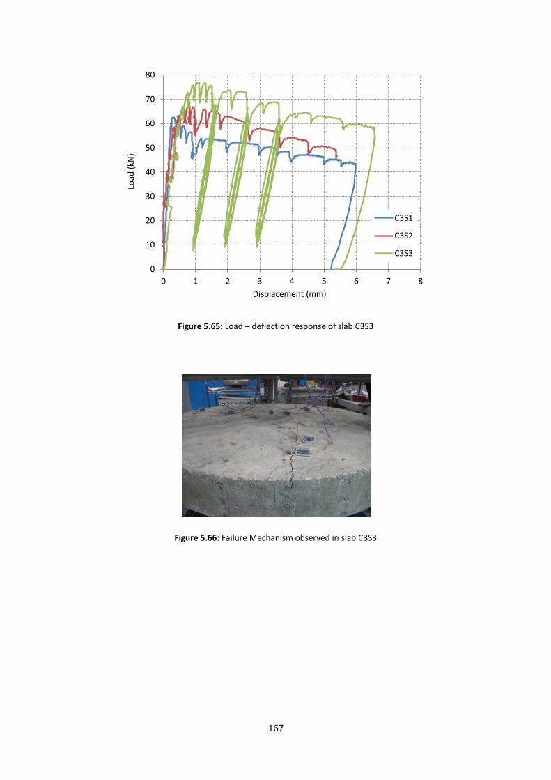
167
Figure 5.65: Load – deflection response of slab C3S3
Figure 5.66: Failure Mechanism observed in slab C3S3
0
10
20
30
40
50
60
70
80
0 1 2 3 4 5 6 7 8
Load
(kN
)
Displacement (mm)
C3S1
C3S2
C3S3

168
(a)
(b)
Figure 5.67: Crack pattern for slab C3S3 (a) photograph (b) angles at which cracks form

169
5.7.3 Crack Width Development
The crack width measurements taken during this test are of particular importance as they provide an
insight into the opening and closing of cracks during loading/unloading. The plate was subjected to a
total of three loading/unloading cycles (Figure 5.65). The slab was unloaded after the displacement
transducers were mounted to give an overlap between the readings of the transducers and the
Demec gauge. Each cycle consisted of three loading/unloading stages. Demec readings were only
taken after the first and third loading/unloading phases. The cycles were initiated at displacements
of 1.5mm, 2.5mm and 3.5mm. Before the initiation of each cycle a set of Demec readings was taken.
The slab was subsequently unloaded to approximately 10kN. Another set of Demec readings were
taken at this point. The slab was then reloaded to the load at the beginning of the cycle.
Figure 5.68 shows the location of the Demec points and the displacement transducers relative to the
location of the cracks. The load – crack width response is shown in Figures 5.69 – 5.71. The
relationship between crack width and displacement for each crack is shown in Figures 5.72 to 5.75,
which show a good agreement between the transducer and Demec readings. Slab C3S3 exhibited a
more symmetrical crack pattern than slabs C3S1 and C3S2 as shown in Figure 5.67. As a result, the
displacement – crack width response of all three cracks is very similar (Figures 5.72 – 5.75). This
shows that although the crack pattern does not affect significantly the overall load-displacement
response, the displacement – crack width relationship is affected.
Figure 5.68: Location of Demec points and transducers in relation to the cracks for slab C3S3
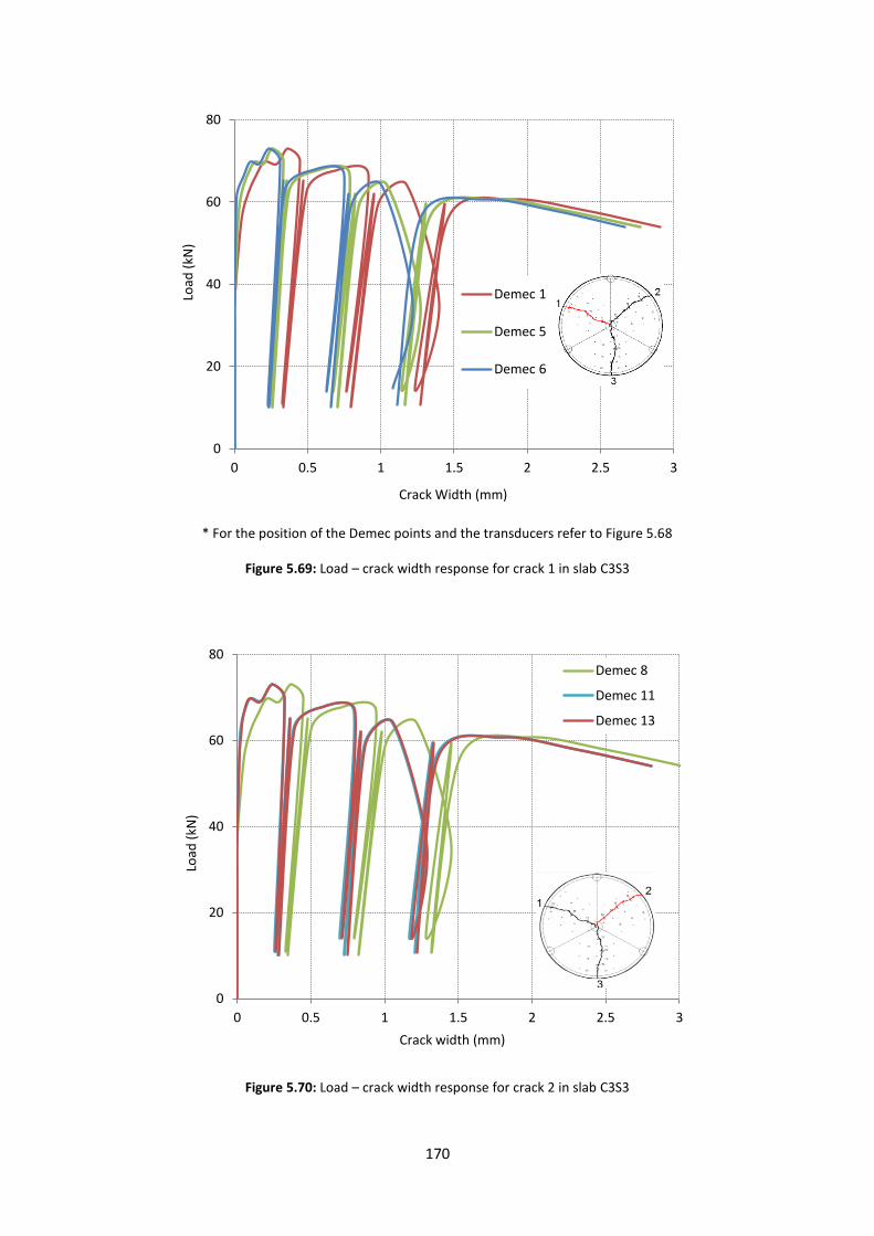
170
* For the position of the Demec points and the transducers refer to Figure 5.68
Figure 5.69: Load – crack width response for crack 1 in slab C3S3
Figure 5.70: Load – crack width response for crack 2 in slab C3S3
0
20
40
60
80
0 0.5 1 1.5 2 2.5 3
Load
(kN
)
Crack Width (mm)
Demec 1
Demec 5
Demec 6
0
20
40
60
80
0 0.5 1 1.5 2 2.5 3
Load
(kN
)
Crack width (mm)
Demec 8
Demec 11
Demec 13
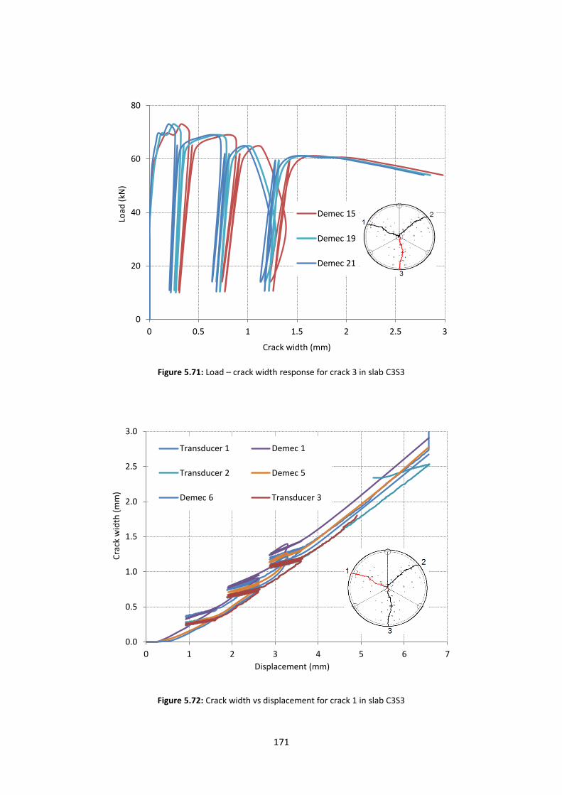
171
Figure 5.71: Load – crack width response for crack 3 in slab C3S3
Figure 5.72: Crack width vs displacement for crack 1 in slab C3S3
0
20
40
60
80
0 0.5 1 1.5 2 2.5 3
Load
(kN
)
Crack width (mm)
Demec 15
Demec 19
Demec 21
0.0
0.5
1.0
1.5
2.0
2.5
3.0
0 1 2 3 4 5 6 7
Cra
ck w
idth
(m
m)
Displacement (mm)
Transducer 1 Demec 1
Transducer 2 Demec 5
Demec 6 Transducer 3

172
Figure 5.73: Crack width vs displacement for crack 2 in slab C3S3
Figure 5.74: Crack width vs displacement for crack 3 in slab C3S3
0.0
0.5
1.0
1.5
2.0
2.5
3.0
3.5
0 1 2 3 4 5 6 7 8
Cra
ck w
idth
(m
m)
Displacement (mm)
Transducer 4
Demec 8
Transducer 5
Demec 11
Demec 13
0.0
0.5
1.0
1.5
2.0
2.5
0 1 2 3 4 5 6 7
Cra
ck w
idth
(m
m)
Displacement (mm)
Demec 21
Transducer 9
Transducer 8
Demec 19
Transducer 7
Demec 15
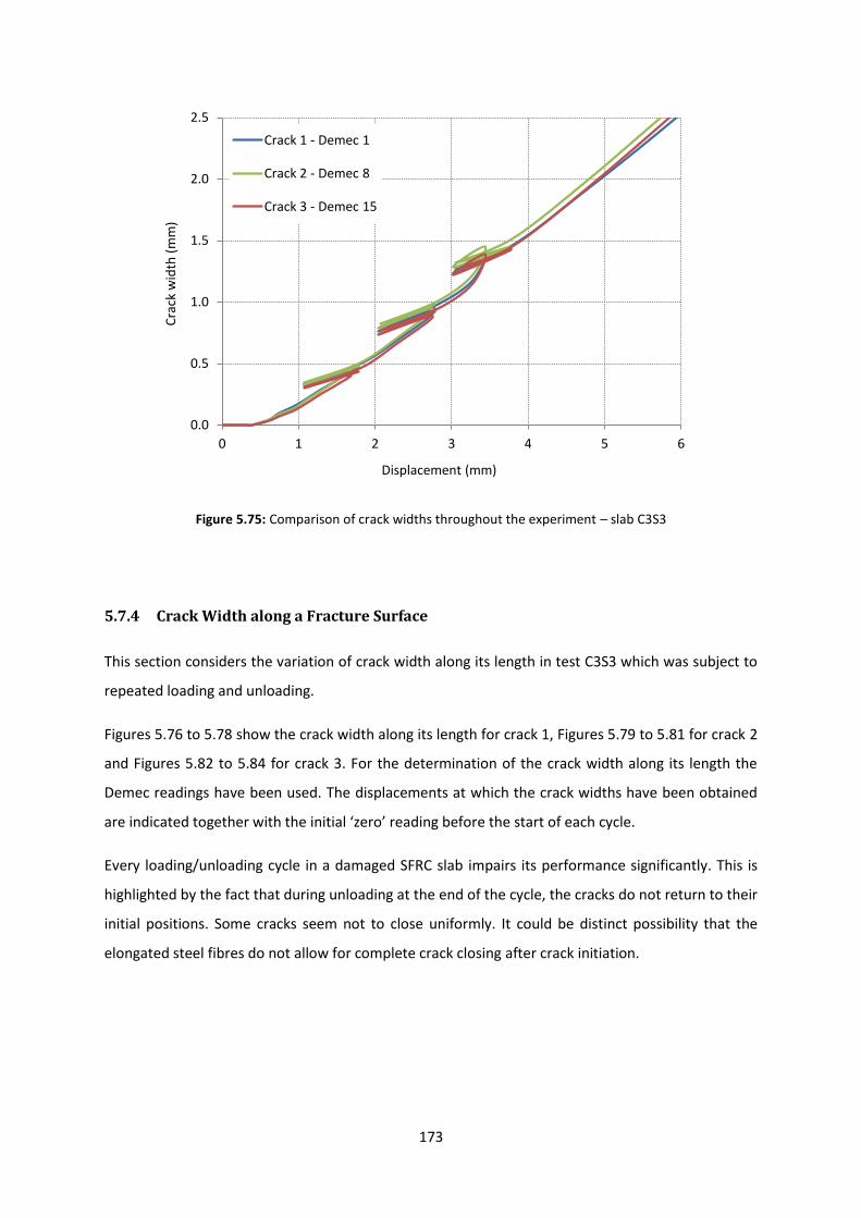
173
Figure 5.75: Comparison of crack widths throughout the experiment – slab C3S3
5.7.4 Crack Width along a Fracture Surface
This section considers the variation of crack width along its length in test C3S3 which was subject to
repeated loading and unloading.
Figures 5.76 to 5.78 show the crack width along its length for crack 1, Figures 5.79 to 5.81 for crack 2
and Figures 5.82 to 5.84 for crack 3. For the determination of the crack width along its length the
Demec readings have been used. The displacements at which the crack widths have been obtained
are indicated together with the initial ‘zero’ reading before the start of each cycle.
Every loading/unloading cycle in a damaged SFRC slab impairs its performance significantly. This is
highlighted by the fact that during unloading at the end of the cycle, the cracks do not return to their
initial positions. Some cracks seem not to close uniformly. It could be distinct possibility that the
elongated steel fibres do not allow for complete crack closing after crack initiation.
0.0
0.5
1.0
1.5
2.0
2.5
0 1 2 3 4 5 6
Cra
ck w
idth
(m
m)
Displacement (mm)
Crack 1 - Demec 1
Crack 2 - Demec 8
Crack 3 - Demec 15

174
*crack width profile at various displacements (in mm)
Figure 5.76: Crack profile – Crack 1 - Cycle 1 (load = 65kN)
Figure 5.77: Crack profile – Crack 1 - Cycle 2 (load = 62 kN)
.
0.0
0.1
0.2
0.3
0.4
0.5
0.6
0 100 200 300 400 500
Cra
ck W
idth
(m
m)
Distance from centre (mm)
1.67mm - zero reading 1.07mm - unloading 1
1.78mm - loading 1 1.08mm - unloading 3
1.79mm - loading 3
0.0
0.2
0.4
0.6
0.8
1.0
1.2
0 100 200 300 400 500
Cra
ck W
idth
(m
m)
Distance from centre (mm)
2.75mm 2.04mm - unloading 1
2.78mm - loading 1 2.07mm - unloading 3
2.80mm - loading 3
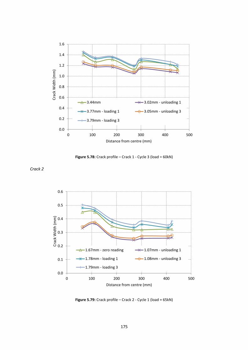
175
Figure 5.78: Crack profile – Crack 1 - Cycle 3 (load = 60kN)
Crack 2
Figure 5.79: Crack profile – Crack 2 - Cycle 1 (load = 65kN)
0.0
0.2
0.4
0.6
0.8
1.0
1.2
1.4
1.6
0 100 200 300 400 500
Cra
ck W
idth
(m
m)
Distance from centre (mm)
3.44mm 3.02mm - unloading 1
3.77mm - loading 1 3.05mm - unloading 3
3.79mm - loading 3
0.0
0.1
0.2
0.3
0.4
0.5
0.6
0 100 200 300 400 500
Cra
ck W
idth
(m
m)
Distance from centre (mm)
1.67mm - zero reading 1.07mm - unloading 1
1.78mm - loading 1 1.08mm - unloading 3
1.79mm - loading 3

176
Figure 5.80: Crack profile – Crack 2 - Cycle 2 (load = 62kN)
Figure 5.81: Crack profile – Crack 2 - Cycle 3 (load = 60kN)
0.0
0.2
0.4
0.6
0.8
1.0
1.2
0 100 200 300 400 500
Cra
ck W
idth
(m
m)
Distance from centre (mm)
2.75mm 2.04mm - unloading 1
2.78mm - loading 1 2.07mm - unloading 3
2.80mm - loading 3
0.0
0.2
0.4
0.6
0.8
1.0
1.2
1.4
1.6
0 100 200 300 400 500
Cra
ck W
idth
(m
m)
Distance from centre (mm)
3.44mm 3.02mm - unloading 1
3.77mm - loading 1 3.05mm - unloading 3
3.79mm - loading 3
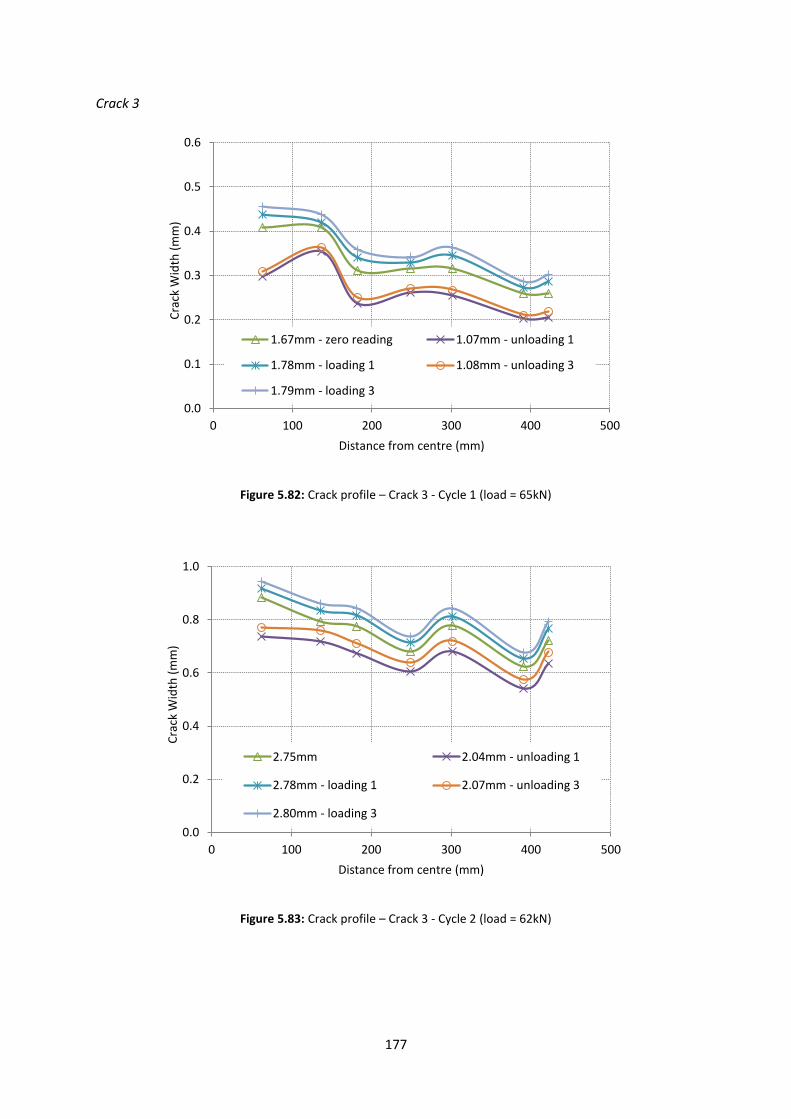
177
Crack 3
Figure 5.82: Crack profile – Crack 3 - Cycle 1 (load = 65kN)
Figure 5.83: Crack profile – Crack 3 - Cycle 2 (load = 62kN)
0.0
0.1
0.2
0.3
0.4
0.5
0.6
0 100 200 300 400 500
Cra
ck W
idth
(m
m)
Distance from centre (mm)
1.67mm - zero reading 1.07mm - unloading 1
1.78mm - loading 1 1.08mm - unloading 3
1.79mm - loading 3
0.0
0.2
0.4
0.6
0.8
1.0
0 100 200 300 400 500
Cra
ck W
idth
(m
m)
Distance from centre (mm)
2.75mm 2.04mm - unloading 1
2.78mm - loading 1 2.07mm - unloading 3
2.80mm - loading 3
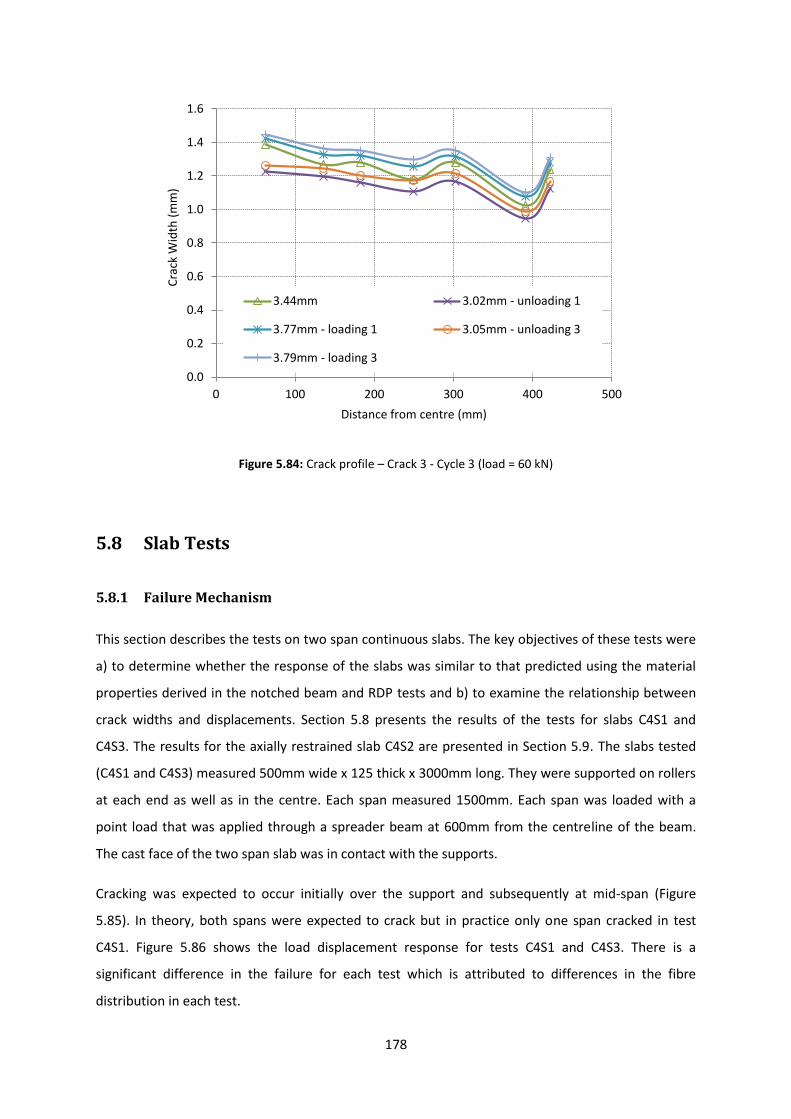
178
Figure 5.84: Crack profile – Crack 3 - Cycle 3 (load = 60 kN)
5.8 Slab Tests
5.8.1 Failure Mechanism
This section describes the tests on two span continuous slabs. The key objectives of these tests were
a) to determine whether the response of the slabs was similar to that predicted using the material
properties derived in the notched beam and RDP tests and b) to examine the relationship between
crack widths and displacements. Section 5.8 presents the results of the tests for slabs C4S1 and
C4S3. The results for the axially restrained slab C4S2 are presented in Section 5.9. The slabs tested
(C4S1 and C4S3) measured 500mm wide x 125 thick x 3000mm long. They were supported on rollers
at each end as well as in the centre. Each span measured 1500mm. Each span was loaded with a
point load that was applied through a spreader beam at 600mm from the centreline of the beam.
The cast face of the two span slab was in contact with the supports.
Cracking was expected to occur initially over the support and subsequently at mid-span (Figure
5.85). In theory, both spans were expected to crack but in practice only one span cracked in test
C4S1. Figure 5.86 shows the load displacement response for tests C4S1 and C4S3. There is a
significant difference in the failure for each test which is attributed to differences in the fibre
distribution in each test.
0.0
0.2
0.4
0.6
0.8
1.0
1.2
1.4
1.6
0 100 200 300 400 500
Cra
ck W
idth
(m
m)
Distance from centre (mm)
3.44mm 3.02mm - unloading 1
3.77mm - loading 1 3.05mm - unloading 3
3.79mm - loading 3
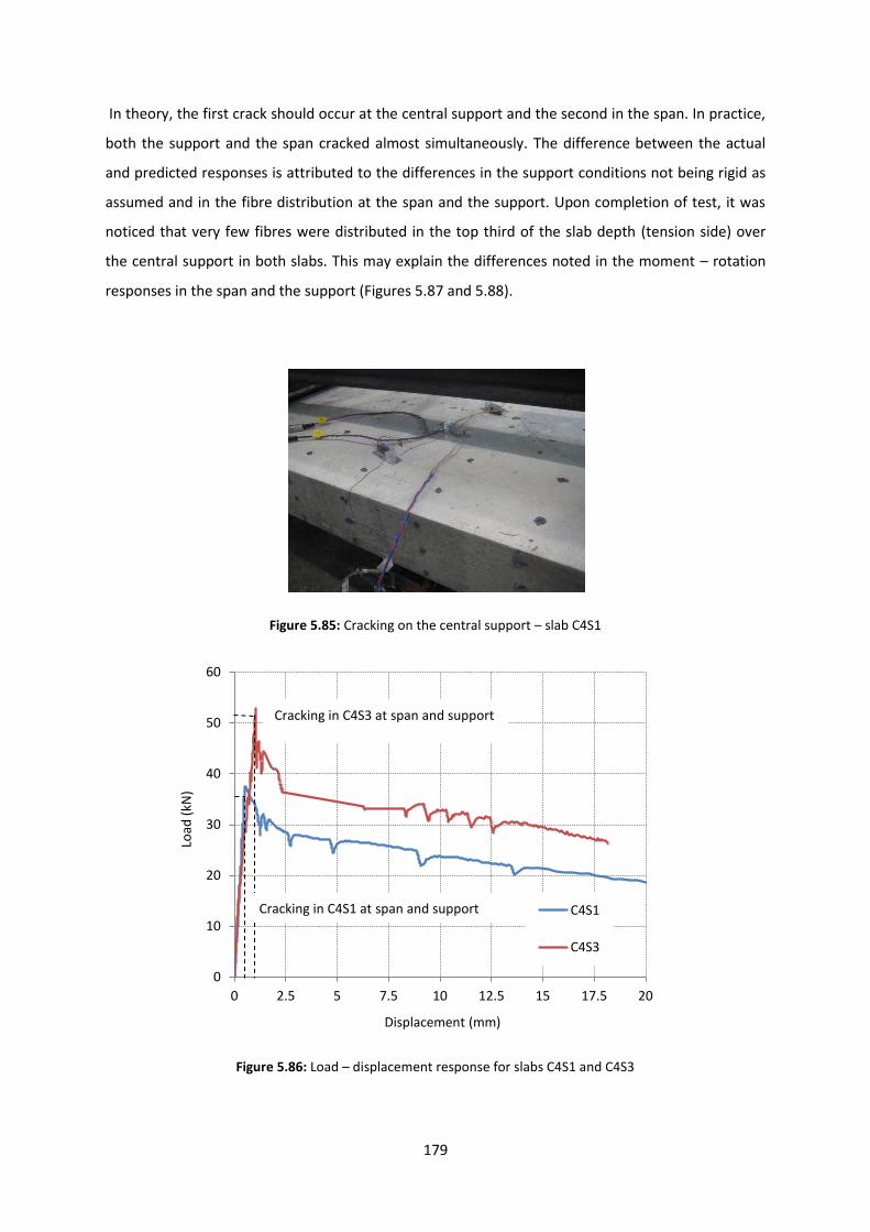
179
In theory, the first crack should occur at the central support and the second in the span. In practice,
both the support and the span cracked almost simultaneously. The difference between the actual
and predicted responses is attributed to the differences in the support conditions not being rigid as
assumed and in the fibre distribution at the span and the support. Upon completion of test, it was
noticed that very few fibres were distributed in the top third of the slab depth (tension side) over
the central support in both slabs. This may explain the differences noted in the moment – rotation
responses in the span and the support (Figures 5.87 and 5.88).
Figure 5.85: Cracking on the central support – slab C4S1
Figure 5.86: Load – displacement response for slabs C4S1 and C4S3
0
10
20
30
40
50
60
0 2.5 5 7.5 10 12.5 15 17.5 20
Load
(kN
)
Displacement (mm)
C4S1
C4S3
Cracking in C4S1 at span and support
Cracking in C4S3 at span and support
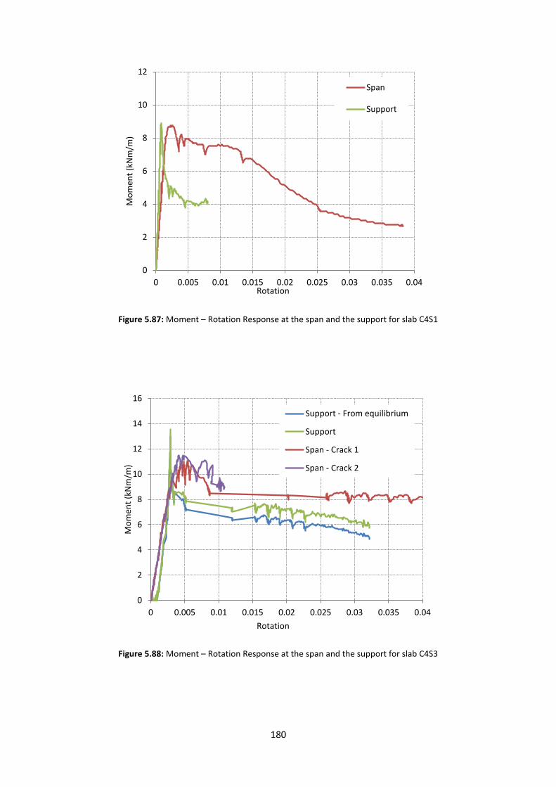
180
Figure 5.87: Moment – Rotation Response at the span and the support for slab C4S1
Figure 5.88: Moment – Rotation Response at the span and the support for slab C4S3
0
2
4
6
8
10
12
0 0.005 0.01 0.015 0.02 0.025 0.03 0.035 0.04
Mo
men
t (k
Nm
/m)
Rotation
Span
Support
0
2
4
6
8
10
12
14
16
0 0.005 0.01 0.015 0.02 0.025 0.03 0.035 0.04
Mo
men
t (k
Nm
/m)
Rotation
Support - From equilibrium
Support
Span - Crack 1
Span - Crack 2
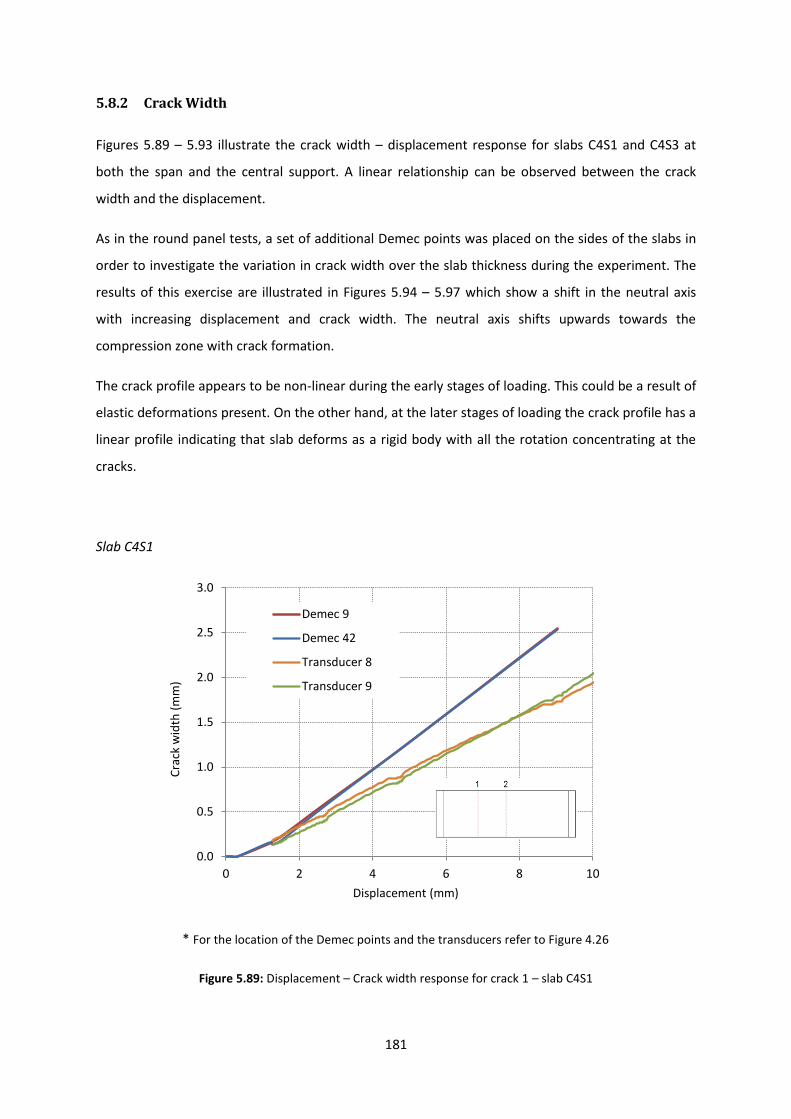
181
5.8.2 Crack Width
Figures 5.89 – 5.93 illustrate the crack width – displacement response for slabs C4S1 and C4S3 at
both the span and the central support. A linear relationship can be observed between the crack
width and the displacement.
As in the round panel tests, a set of additional Demec points was placed on the sides of the slabs in
order to investigate the variation in crack width over the slab thickness during the experiment. The
results of this exercise are illustrated in Figures 5.94 – 5.97 which show a shift in the neutral axis
with increasing displacement and crack width. The neutral axis shifts upwards towards the
compression zone with crack formation.
The crack profile appears to be non-linear during the early stages of loading. This could be a result of
elastic deformations present. On the other hand, at the later stages of loading the crack profile has a
linear profile indicating that slab deforms as a rigid body with all the rotation concentrating at the
cracks.
Slab C4S1
* For the location of the Demec points and the transducers refer to Figure 4.26
Figure 5.89: Displacement – Crack width response for crack 1 – slab C4S1
0.0
0.5
1.0
1.5
2.0
2.5
3.0
0 2 4 6 8 10
Cra
ck w
idth
(m
m)
Displacement (mm)
Demec 9
Demec 42
Transducer 8
Transducer 9
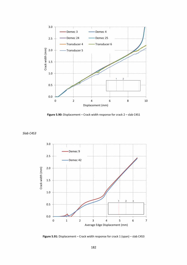
182
Figure 5.90: Displacement – Crack width response for crack 2 – slab C4S1
Slab C4S3
Figure 5.91: Displacement – Crack width response for crack 1 (span) – slab C4S3
0.0
0.5
1.0
1.5
2.0
2.5
3.0
0 2 4 6 8 10
Cra
ck w
idth
(m
m)
Displacement (mm)
Demec 3 Demec 4
Demec 24 Demec 25
Transducer 4 Transducer 6
Transducer 5
0.0
0.5
1.0
1.5
2.0
2.5
3.0
0 1 2 3 4 5 6 7
Cra
ck w
idth
(m
m)
Average Edge Displacement (mm)
Demec 9
Demec 42
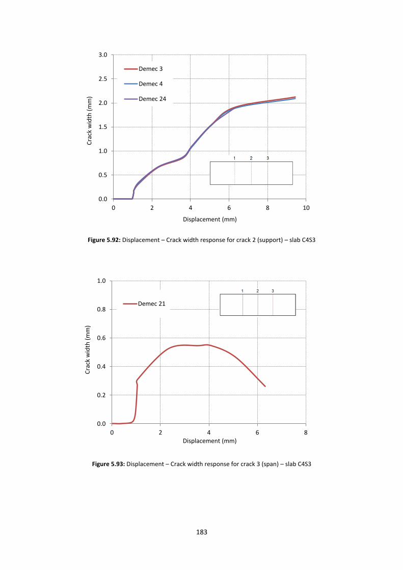
183
Figure 5.92: Displacement – Crack width response for crack 2 (support) – slab C4S3
Figure 5.93: Displacement – Crack width response for crack 3 (span) – slab C4S3
0.0
0.5
1.0
1.5
2.0
2.5
3.0
0 2 4 6 8 10
Cra
ck w
idth
(m
m)
Displacement (mm)
Demec 3
Demec 4
Demec 24
0.0
0.2
0.4
0.6
0.8
1.0
0 2 4 6 8
Cra
ck w
idth
(m
m)
Displacement (mm)
Demec 21

184
Slab C4S1
*crack width profile plotted at various displacements (in mm)
Figure 5.94: Crack width profile at span (crack 1)
Figure 5.95: Crack width profile at support (crack 2)
0
25
50
75
100
125
0.0 0.5 1.0 1.5 2.0 2.5 3.0
Dep
th t
hro
ugh
sla
b (
mm
)
Crack Width (mm)
1.19mm
1.26mm
1.54mm
2.72mm
4.80mm
9.05mm
0
25
50
75
100
125
0.0 0.5 1.0 1.5 2.0
Dep
th t
hro
ugh
sla
b (
mm
)
Crack Width (mm)
1.19mm
1.26mm
1.54mm
2.72mm
4.80mm
9.05mm

185
Slab C4S3
*crack width profile plotted at various displacements
Figure 5.96: Crack width profile at span (crack 1)
Figure 5.97: Crack width profile at support (crack 2)
0
25
50
75
100
125
0.0 0.2 0.4 0.6 0.8 1.0 1.2
Dep
th t
hro
ugh
sla
b (
mm
)
Crack Width (mm)
0.83mm
0.97mm
1.05mm
2.33mm
4.09mm
0
25
50
75
100
125
0.0 0.2 0.4 0.6 0.8 1.0 1.2
Dep
th t
hro
ugh
sla
b (
mm
)
Crack Width (mm)
0.83mm
0.97mm
1.05mm
2.33mm
4.09mm
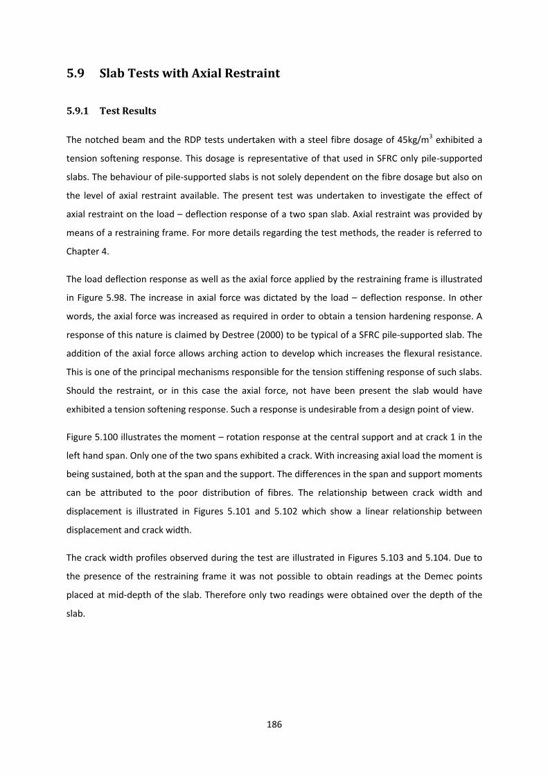
186
5.9 Slab Tests with Axial Restraint
5.9.1 Test Results
The notched beam and the RDP tests undertaken with a steel fibre dosage of 45kg/m3 exhibited a
tension softening response. This dosage is representative of that used in SFRC only pile-supported
slabs. The behaviour of pile-supported slabs is not solely dependent on the fibre dosage but also on
the level of axial restraint available. The present test was undertaken to investigate the effect of
axial restraint on the load – deflection response of a two span slab. Axial restraint was provided by
means of a restraining frame. For more details regarding the test methods, the reader is referred to
Chapter 4.
The load deflection response as well as the axial force applied by the restraining frame is illustrated
in Figure 5.98. The increase in axial force was dictated by the load – deflection response. In other
words, the axial force was increased as required in order to obtain a tension hardening response. A
response of this nature is claimed by Destree (2000) to be typical of a SFRC pile-supported slab. The
addition of the axial force allows arching action to develop which increases the flexural resistance.
This is one of the principal mechanisms responsible for the tension stiffening response of such slabs.
Should the restraint, or in this case the axial force, not have been present the slab would have
exhibited a tension softening response. Such a response is undesirable from a design point of view.
Figure 5.100 illustrates the moment – rotation response at the central support and at crack 1 in the
left hand span. Only one of the two spans exhibited a crack. With increasing axial load the moment is
being sustained, both at the span and the support. The differences in the span and support moments
can be attributed to the poor distribution of fibres. The relationship between crack width and
displacement is illustrated in Figures 5.101 and 5.102 which show a linear relationship between
displacement and crack width.
The crack width profiles observed during the test are illustrated in Figures 5.103 and 5.104. Due to
the presence of the restraining frame it was not possible to obtain readings at the Demec points
placed at mid-depth of the slab. Therefore only two readings were obtained over the depth of the
slab.

187
Figure 5.98: Load – Deflection response of slab C4S2
Figure 5.99: Load – Deflection response of slabs C4S1, C4S2 and C4S3
0
10
20
30
40
50
60
0 2.5 5 7.5 10 12.5 15 17.5
Load
(kN
)
Displacement (mm)
Load (kN)
Axial Force (kN)
0
10
20
30
40
50
60
0 2.5 5 7.5 10 12.5 15 17.5 20
Load
(kN
)
Displacement (mm)
C4S1
C4S2
C4S3
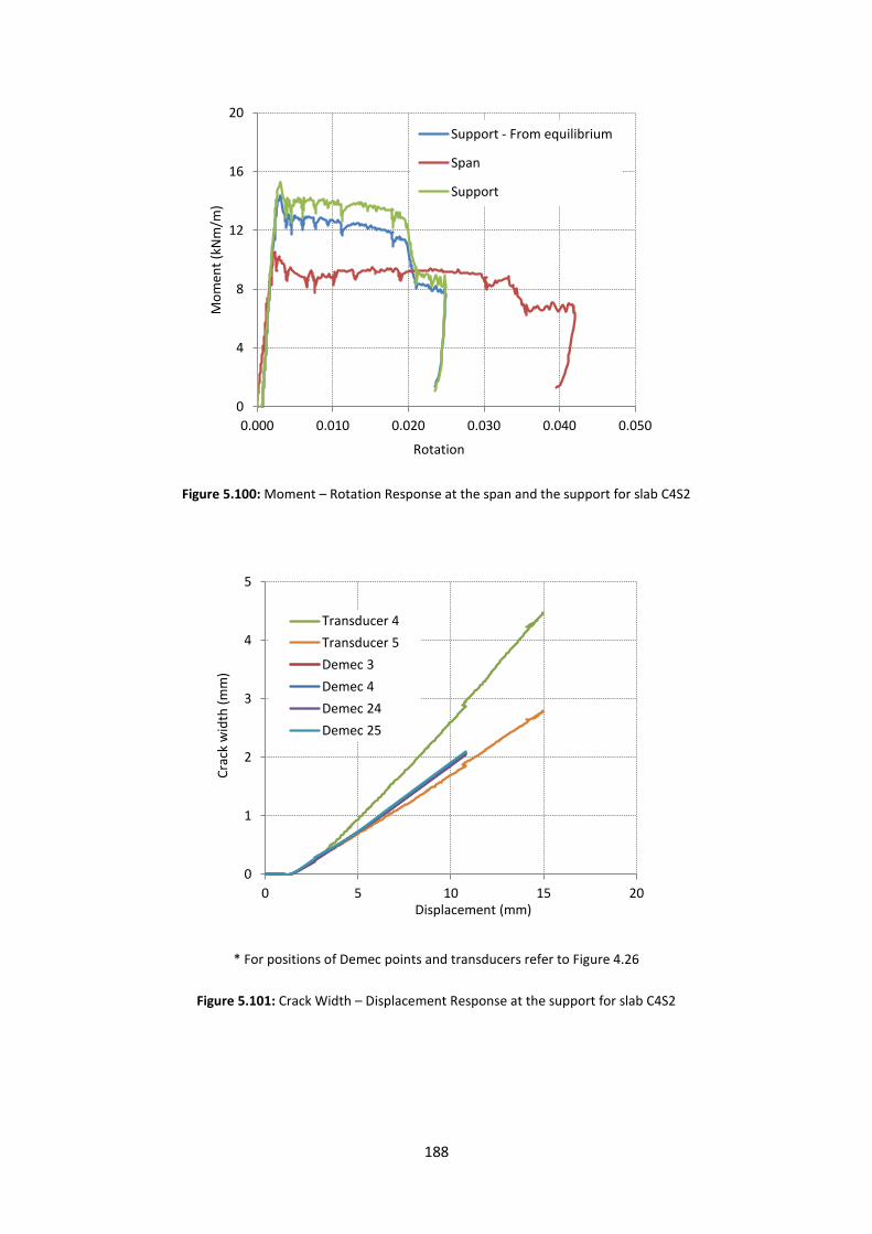
188
Figure 5.100: Moment – Rotation Response at the span and the support for slab C4S2
* For positions of Demec points and transducers refer to Figure 4.26
Figure 5.101: Crack Width – Displacement Response at the support for slab C4S2
0
4
8
12
16
20
0.000 0.010 0.020 0.030 0.040 0.050
Mo
men
t (k
Nm
/m)
Rotation
Support - From equilibrium
Span
Support
0
1
2
3
4
5
0 5 10 15 20
Cra
ck w
idth
(m
m)
Displacement (mm)
Transducer 4
Transducer 5
Demec 3
Demec 4
Demec 24
Demec 25

189
Figure 5.102: Crack Width – Displacement Response at the span for slab C4S2
* Crack width profile through the depth plotted at various displacements (in mm)
Figure 5.103: Crack Width Profile at the span – slab C4S2
0
1
2
3
4
5
6
0 5 10 15 20
Cra
ck w
idth
(m
m)
Displacement (mm)
Transducer 3
Transducer 6
Demec 9
Demec 42
0
25
50
75
100
125
0.0 0.4 0.8 1.2 1.6 2.0
Dep
th t
hro
ugh
sla
b (
mm
)
Crack Width (mm)
0.88mm
1.40mm
2.69mm
2.70mm
4.64mm
6.73mm
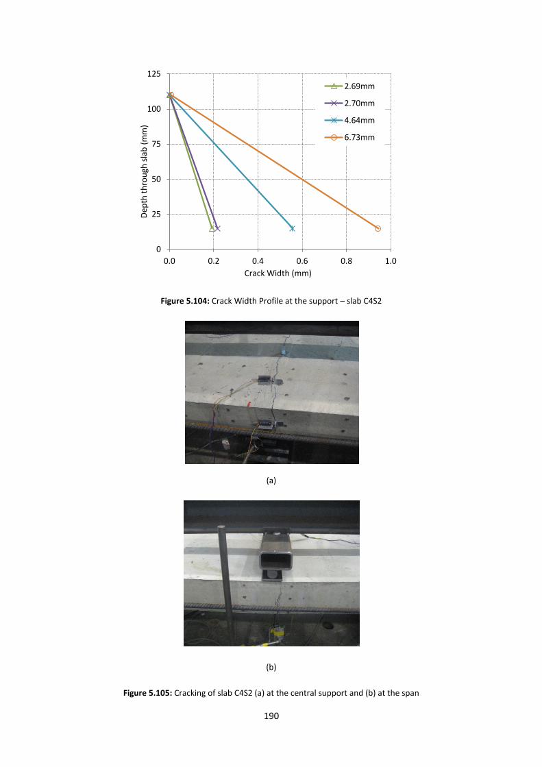
190
Figure 5.104: Crack Width Profile at the support – slab C4S2
(a)
(b)
Figure 5.105: Cracking of slab C4S2 (a) at the central support and (b) at the span
0
25
50
75
100
125
0.0 0.2 0.4 0.6 0.8 1.0
Dep
th t
hro
ugh
sla
b (
mm
)
Crack Width (mm)
2.69mm
2.70mm
4.64mm
6.73mm

191
5.10 Punching Shear Tests
5.10.1 Test Results
Two types of punching tests were carried out as part of the present research on behalf of Abbey
Pynford. The type I punching tests were reinforced with one hoop of steel reinforcement whereas
Type II incorporated two hoops of steel reinforcement. Self-compacting concrete with compressive
strength of 70MPa was used along with a fibre dosage of 50kg/m3. The methodology for the
punching shear tests is described in more detail in Section 4.10. The results obtained from these
tests are illustrated in Figures 5.106 to 5.108. RDP tests were carried out for all the fibres in order to
obtain the material properties. As expected, the plain concrete plates exhibited a very brittle post-
cracking response due to the absence of steel fibres. The addition of fibres increased the peak
strength by around 40%. In addition, fibres significantly improve the post-peak response through
crack bridging and crack arrest mechanisms.
The plates reinforced with one hoop exhibited a mixture of flexural and punching failure as shown by
the ductile nature of the load displacement response (Figure 5.107). On the other hand, the plates
reinforced with two hoops exhibited a punching type of failure (Figure 5.109). All three types of
fibres tested offer similar peak loads for both the Type I and Type II tests. However, the helical fibres
appear to offer more ductility, particularly for the Type II punching shear tests. The analysis of the
present punching shear tests is undertaken in Chapter 7 (Section 7.6).
Figure 5.106: Load displacement in Flexural Tests
0
20
40
60
80
100
120
0 5 10 15 20
Load
[kN
]
Central displacement [mm]
Flexure helix
flexure 55/35 fibre
Flexure 75/35 fibre
Plain concrete

192
Figure 5.107: Load displacement in Type I Punching Shear Tests
Figure 5.108: Load displacement in Type II Punching Shear Tests
0
50
100
150
200
250
300
0 5 10 15 20 25
Load
[kN
]
Central displacement [mm]
Plain concrete 1 hoop
75/35 fibre: 1 hoop
55/35 fibre: 1 hoop
Helix 1 hoop
0
50
100
150
200
250
300
350
0 2.5 5 7.5 10 12.5 15
Load
[kN
]
Central displacement [mm]
55/35 fibre: 2 hoop Plain concrete 2 hoop 75/35 fibre: 2 hoops Helix: 2 hoop
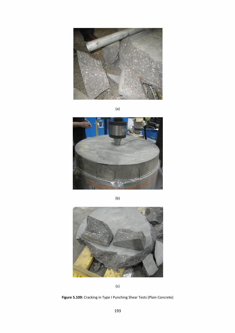
193
(a)
(b)
(c)
Figure 5.109: Cracking in Type I Punching Shear Tests (Plain Concrete)
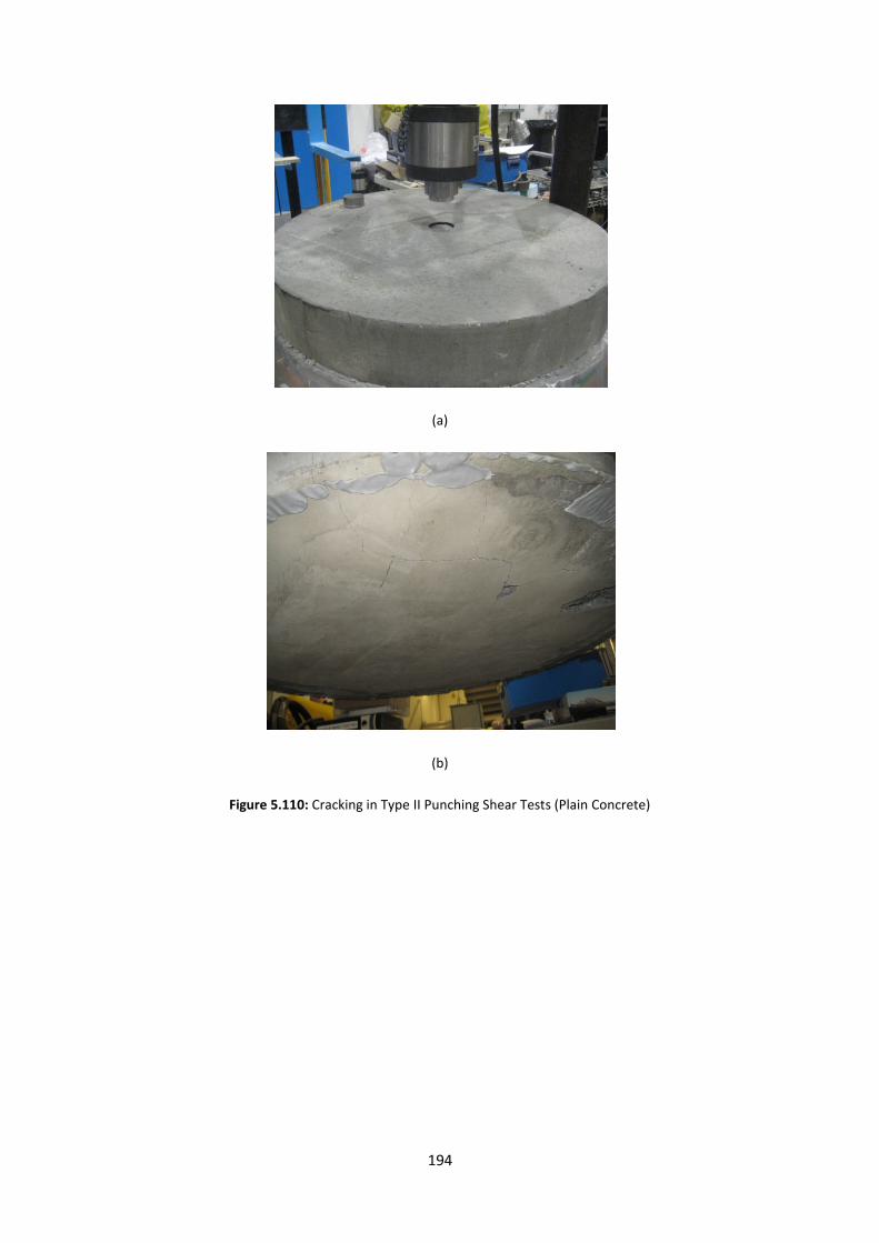
194
(a)
(b)
Figure 5.110: Cracking in Type II Punching Shear Tests (Plain Concrete)
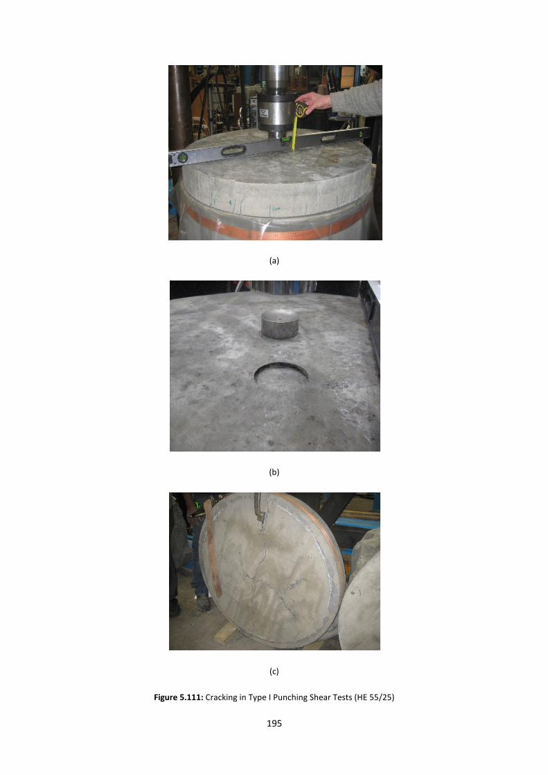
195
(a)
(b)
(c)
Figure 5.111: Cracking in Type I Punching Shear Tests (HE 55/25)
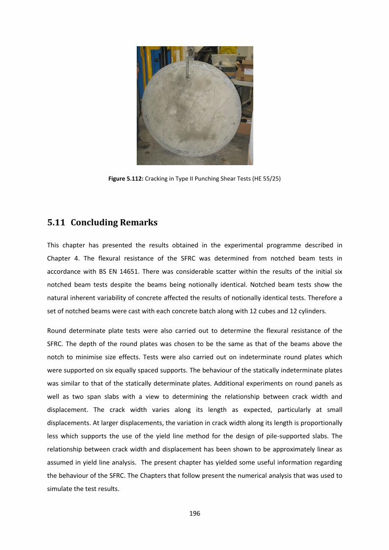
196
Figure 5.112: Cracking in Type II Punching Shear Tests (HE 55/25)
5.11 Concluding Remarks
This chapter has presented the results obtained in the experimental programme described in
Chapter 4. The flexural resistance of the SFRC was determined from notched beam tests in
accordance with BS EN 14651. There was considerable scatter within the results of the initial six
notched beam tests despite the beams being notionally identical. Notched beam tests show the
natural inherent variability of concrete affected the results of notionally identical tests. Therefore a
set of notched beams were cast with each concrete batch along with 12 cubes and 12 cylinders.
Round determinate plate tests were also carried out to determine the flexural resistance of the
SFRC. The depth of the round plates was chosen to be the same as that of the beams above the
notch to minimise size effects. Tests were also carried out on indeterminate round plates which
were supported on six equally spaced supports. The behaviour of the statically indeterminate plates
was similar to that of the statically determinate plates. Additional experiments on round panels as
well as two span slabs with a view to determining the relationship between crack width and
displacement. The crack width varies along its length as expected, particularly at small
displacements. At larger displacements, the variation in crack width along its length is proportionally
less which supports the use of the yield line method for the design of pile-supported slabs. The
relationship between crack width and displacement has been shown to be approximately linear as
assumed in yield line analysis. The present chapter has yielded some useful information regarding
the behaviour of the SFRC. The Chapters that follow present the numerical analysis that was used to
simulate the test results.

197
Chapter Six
Numerical Methodology
6.1 General Remarks
The present chapter gives a detailed description of the numerical methods of analysis used in
Chapters 7 and 8 of the present thesis. A brief account of the different constitutive concrete models
is given as well as a more detailed description of the preferred approach.
6.2 Review of the Finite Element Method
6.2.1 Linear Finite Element Analysis
In contemporary engineering, there exist numerous complex structural problems. In many cases
their immense complexity does not allow for the development of analytical solutions, for a variety of
reasons such as geometric and material non-linearities. This has led to the development of the finite
element method. Since, its introduction in the early 1950s, the finite element method (FEM) has
been used extensively both for research and design.
This method involves ‘breaking down’ the structure into discrete elements, thus shifting the focus of
attention from a continuum to a discrete domain. The element is comprised of nodes, which are
positioned at the inter-element boundaries, and in some cases inside the element. The behaviour of
each element is expressed in terms of its nodal displacements. In turn the inter-nodal behaviour is
defined by the use of appropriate shape functions.
u N d (6.1)
In the above expression, u denotes the matrix defining the displacements within an element N
denotes the shape functions matrix and d denotes the nodal displacement matrix.
Consequently, the strains can be derived from the following equation:
u B d (6.2)
where, denotes the strain matrix and B is defined as follows:
198
B N (6.3)
The stresses and strains within each element obey the following relation:
D (6.4)
where, and are the stress and strain matrices; whereas D denotes the matrix of the
constitutive relation between the stress and the strain. The constitutive relationship matrix can be
defined in accordance to the material behaviour considered (isotropic, anisotropic, linear, etc.).
The stresses can therefore be related to the nodal displacements, by substituting equation (6.2) into
equation (6.4).
D B d (6.5)
The concept of Virtual Work can then be used, to define the local stiffness matrix. This matrix relates
the external loads to the nodal displacements computed in equation (6.5).
Consider an external virtual force, F applied to a specified node. The internal work dissipated inside
the element can be computed as follows:
T
wI dV (6.6)
Furthermore, the internal work equation can be expressed in terms of the nodal displacements, by
simple substitution of equations (6.5) and (6.2) into equation (6.6).
T
wI B d D B d dV (6.7)
The external work, can then be derived:
T
wE d F (6.8)
where, T
d denotes the transpose of the nodal displacement matrix and F denotes the matrix of
external forces applied onto the element under consideration.
To achieve equilibrium conditions the total potential energy within the system must equal to zero.
Therefore, axiomatically the internal and external energies of the system must be equal:
TT
d F B d D B d dV (6.9)
199
By manipulating equation (6.9) to express the external force in terms of the nodal displacements, we
obtain:
T
F B D B d dV (6.10)
Equation (6.10) can also be expressed as:
F K d dV (6.11)
where, K denotes the stiffness matrix and is defined as:
T
K B D B dV (6.12)
The stiffness matrix needs to be transformed from the local element axes to the global axes before
assembling the stiffness matrix. Equation (6.12) is then solved, by numerical integration over a finite
number of points in order to obtain the forces and the nodal displacements associated with the
system.
The present sub-section has served in providing a brief overview of the linear finite element analysis
method. For a more in-depth discussion of the methods outlined above the interested reader is
referred to specialist finite element analysis textbooks such as (Zienkiewicz & Taylor, 1989).
6.2.2 Non-Linear Finite Element Analysis
The post-cracking behaviour of concrete is characterised by a non-linear response due to material
nonlinearity. Additionally, geometric non-linearities can arise if the geometrical arrangement of the
structure changes significantly during loading (Kotsovos & Pavlovic, 1995) (Zienkiewicz & Taylor,
1989). The influence of geometrical nonlinearity is usually small for concrete structures but can
become significant when crack widths are large compared with the element size (Tlemat, Pilakoutas,
& Neocleous, 2006).
Problems involving material and/or geometric non-linearities are solved using the incremental
iterative method . This method involves the load being applied in small increments. The solutions are
obtained using iterations until a sufficient level of accuracy is achieved. The philosophy behind this
approach involved in evaluating the load system from the stresses within the structure. The
evaluated load system is then compared with the applied load system. This results in a set of
residual forces which are then applied onto the structure to satisfy equilibrium. The process
continues until the residual forces meet pre specified converge criteria.
200
This is the procedure adopted for the present study. This procedure native to ABAQUS is described
in more detail within section 6.3.4. The constitutive model adopted is described in section 6.5.
6.3 Constitutive Modelling Approaches in NLFEA
6.3.1 General Overview
Modelling the post-cracking behaviour of concrete is a ‘challenging’ task. The load-deflection
response of concrete after cracking (both in tension and compression) is inherently non-linear.
Geometric non-linearities need to be introduced if the crack width is large compared to the element
size. The progression of existing cracks and the formation of additional ones can contribute to the
difficulties in the application of the FEM to the modelling of concrete structures.
Numerical approaches for modelling the onset and propagation of cracking in concrete can
essentially be divided into two main categories; discrete and smeared cracking.
6.3.2 Discrete cracking
The concept of the numerical simulation of concrete fracture using a discrete cracking formulation
was introduced in 1967 by Ngo and Scordelis (1967). This approach involves introducing a crack as a
‘geometric entity’ (de Borst, Remmers, Needleman, & Abellan, 2004) at a pre-specified location.
When the force at the node exceeds a pre-specified strength criterion, then the crack grows.
Consequently, the node is split into two, as the crack propagates (Figure 6.1). The same process
occurs for the remaining nodes.
Such a method is very appealing for the study of individual cracks. It can be argued that such a
method will yield a reasonable approximation of the concrete cracking process (Ngo & Scordelis,
1967). However, there are a number of distinct drawbacks in using such a method. Primarily, the
location of the cracks has to be pre-determined. For statically indeterminate structures, this can be
challenging. Furthermore, the additional refinements of the mesh required, as well as the constantly
changing boundary conditions can create a model that is difficult to handle numerically.
Secondly, cracks have to propagate along element boundaries thus creating a mesh bias (de Borst,
Remmers, Needleman, & Abellan, 2004). Automatic re-meshing can reduce the mesh bias
significantly, but would make this process even more computationally expensive. In addition, the
change in topology due to the crack can be very difficult to handle numerically (de Borst, Remmers,
Needleman, & Abellan, 2004).
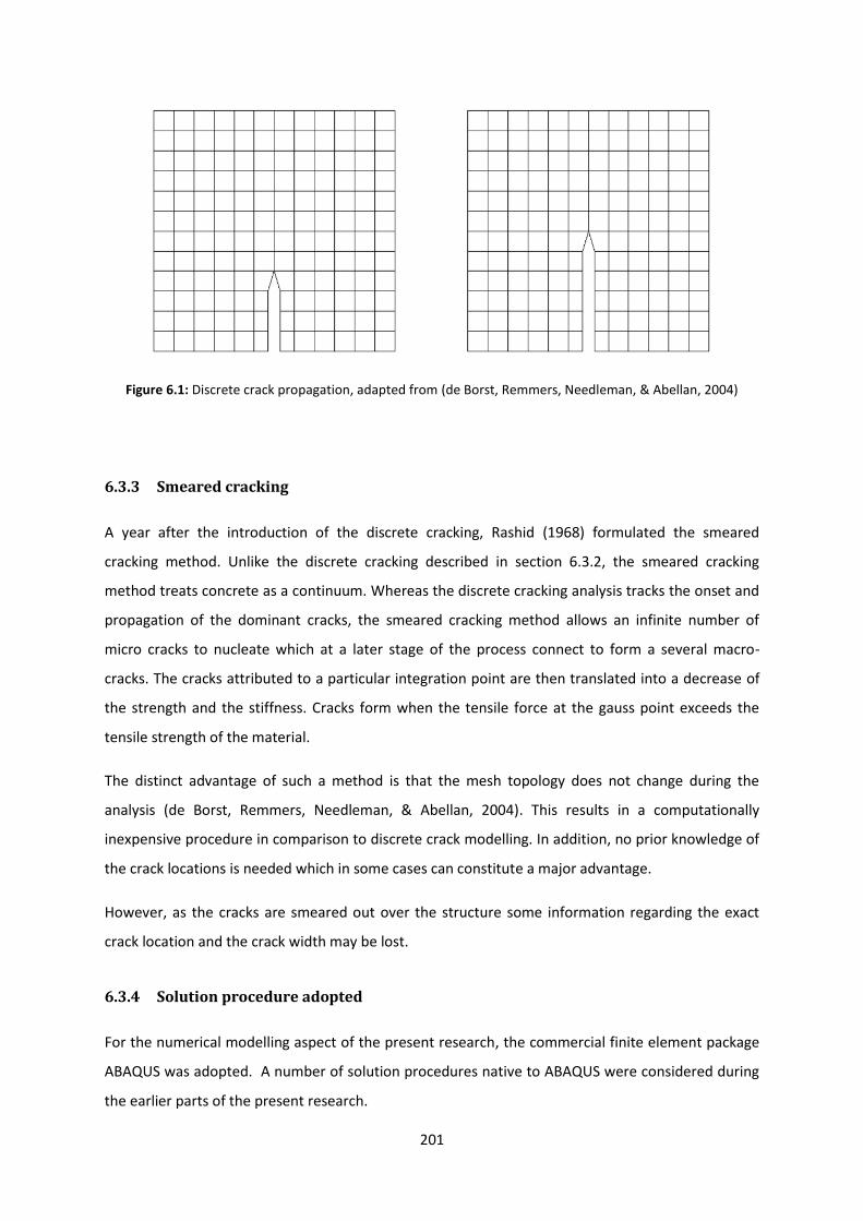
201
Figure 6.1: Discrete crack propagation, adapted from (de Borst, Remmers, Needleman, & Abellan, 2004)
6.3.3 Smeared cracking
A year after the introduction of the discrete cracking, Rashid (1968) formulated the smeared
cracking method. Unlike the discrete cracking described in section 6.3.2, the smeared cracking
method treats concrete as a continuum. Whereas the discrete cracking analysis tracks the onset and
propagation of the dominant cracks, the smeared cracking method allows an infinite number of
micro cracks to nucleate which at a later stage of the process connect to form a several macro-
cracks. The cracks attributed to a particular integration point are then translated into a decrease of
the strength and the stiffness. Cracks form when the tensile force at the gauss point exceeds the
tensile strength of the material.
The distinct advantage of such a method is that the mesh topology does not change during the
analysis (de Borst, Remmers, Needleman, & Abellan, 2004). This results in a computationally
inexpensive procedure in comparison to discrete crack modelling. In addition, no prior knowledge of
the crack locations is needed which in some cases can constitute a major advantage.
However, as the cracks are smeared out over the structure some information regarding the exact
crack location and the crack width may be lost.
6.3.4 Solution procedure adopted
For the numerical modelling aspect of the present research, the commercial finite element package
ABAQUS was adopted. A number of solution procedures native to ABAQUS were considered during
the earlier parts of the present research.
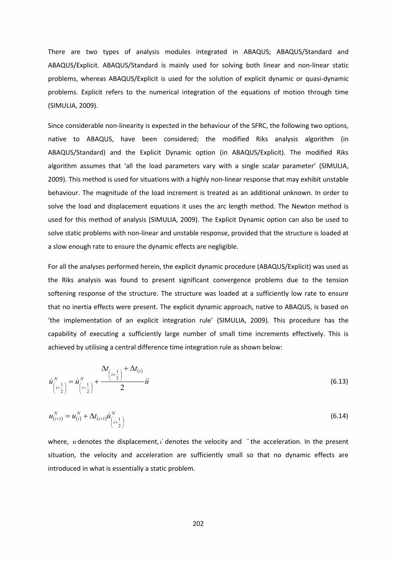
202
There are two types of analysis modules integrated in ABAQUS; ABAQUS/Standard and
ABAQUS/Explicit. ABAQUS/Standard is mainly used for solving both linear and non-linear static
problems, whereas ABAQUS/Explicit is used for the solution of explicit dynamic or quasi-dynamic
problems. Explicit refers to the numerical integration of the equations of motion through time
(SIMULIA, 2009).
Since considerable non-linearity is expected in the behaviour of the SFRC, the following two options,
native to ABAQUS, have been considered; the modified Riks analysis algorithm (in
ABAQUS/Standard) and the Explicit Dynamic option (in ABAQUS/Explicit). The modified Riks
algorithm assumes that ‘all the load parameters vary with a single scalar parameter’ (SIMULIA,
2009). This method is used for situations with a highly non-linear response that may exhibit unstable
behaviour. The magnitude of the load increment is treated as an additional unknown. In order to
solve the load and displacement equations it uses the arc length method. The Newton method is
used for this method of analysis (SIMULIA, 2009). The Explicit Dynamic option can also be used to
solve static problems with non-linear and unstable response, provided that the structure is loaded at
a slow enough rate to ensure the dynamic effects are negligible.
For all the analyses performed herein, the explicit dynamic procedure (ABAQUS/Explicit) was used as
the Riks analysis was found to present significant convergence problems due to the tension
softening response of the structure. The structure was loaded at a sufficiently low rate to ensure
that no inertia effects were present. The explicit dynamic approach, native to ABAQUS, is based on
‘the implementation of an explicit integration rule’ (SIMULIA, 2009). This procedure has the
capability of executing a sufficiently large number of small time increments effectively. This is
achieved by utilising a central difference time integration rule as shown below:
u
tt
uu
ii
N
i
N
i
2
2
1
2
1
2
1
(6.13)
N
ii
N
i
N
i utuu
2
111 (6.14)
where, u denotes the displacement,u denotes the velocity and u the acceleration. In the present
situation, the velocity and acceleration are sufficiently small so that no dynamic effects are
introduced in what is essentially a static problem.
203
The efficiency by using this approach lies, not with the fact that an explicit integration rule is used
but rather with the fact that a diagonal mass matrix is adopted (SIMULIA, 2009). The accelerations at
the beginning of each separate time step are computed as follows:
JiJ
i
NJN
i IPMu 1
(6.15)
where, NJM is the mass matrix, J
iP is the load vector and
J
iI is the internal force vector.
6.4 Constitutive Modelling Approaches Adopted
6.4.1 Introduction to Concrete Constitutive Modelling Approaches
The finite element analysis modelling of steel fibre reinforced concrete structures is complex, as
illustrated above. Within ABAQUS, three concrete constitutive modelling approaches are
encompassed based on the smeared crack approach; each representing a different philosophy. A
concise description of these approaches is presented within the following sub-sections of the
present thesis. For a more in-depth discussion of the underlying principles, the interested reader is
referred to the ABAQUS 6.9.1 Theory Manual (SIMULIA, 2009).
6.4.2 Concrete Smeared Cracking (Inelastic Constitutive Model)
The first modelling approach described herein, is the so-called concrete smeared cracking. This
model has been primarily developed for use in structural problems exhibiting ‘monotonic loadings
under low confined pressures’ (SIMULIA, 2009). Furthermore, as explained in Section 2.5.4., it
utilises the crack band width philosophy as postulated by Bazant and Oh (1983). The primary
assumption made, under this constitutive philosophy, is that the concrete behaviour is strongly
dominated by cracking. The compression and the cracking behaviour, associated with this model are
defined in terms of its uni-axial response, as depicted in Figure 6.2.
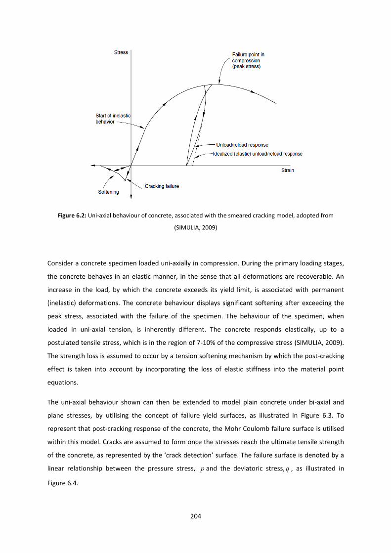
204
Figure 6.2: Uni-axial behaviour of concrete, associated with the smeared cracking model, adopted from
(SIMULIA, 2009)
Consider a concrete specimen loaded uni-axially in compression. During the primary loading stages,
the concrete behaves in an elastic manner, in the sense that all deformations are recoverable. An
increase in the load, by which the concrete exceeds its yield limit, is associated with permanent
(inelastic) deformations. The concrete behaviour displays significant softening after exceeding the
peak stress, associated with the failure of the specimen. The behaviour of the specimen, when
loaded in uni-axial tension, is inherently different. The concrete responds elastically, up to a
postulated tensile stress, which is in the region of 7-10% of the compressive stress (SIMULIA, 2009).
The strength loss is assumed to occur by a tension softening mechanism by which the post-cracking
effect is taken into account by incorporating the loss of elastic stiffness into the material point
equations.
The uni-axial behaviour shown can then be extended to model plain concrete under bi-axial and
plane stresses, by utilising the concept of failure yield surfaces, as illustrated in Figure 6.3. To
represent that post-cracking response of the concrete, the Mohr Coulomb failure surface is utilised
within this model. Cracks are assumed to form once the stresses reach the ultimate tensile strength
of the concrete, as represented by the ‘crack detection’ surface. The failure surface is denoted by a
linear relationship between the pressure stress, p and the deviatoric stress, q , as illustrated in
Figure 6.4.
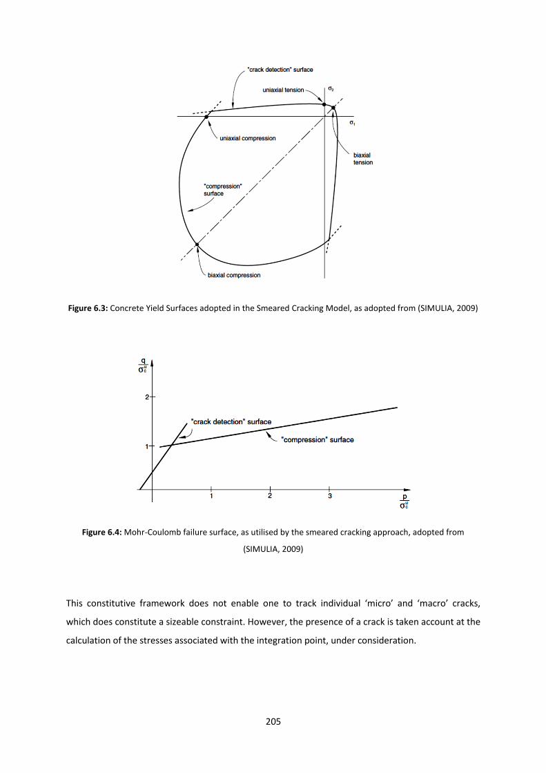
205
Figure 6.3: Concrete Yield Surfaces adopted in the Smeared Cracking Model, as adopted from (SIMULIA, 2009)
Figure 6.4: Mohr-Coulomb failure surface, as utilised by the smeared cracking approach, adopted from
(SIMULIA, 2009)
This constitutive framework does not enable one to track individual ‘micro’ and ‘macro’ cracks,
which does constitute a sizeable constraint. However, the presence of a crack is taken account at the
calculation of the stresses associated with the integration point, under consideration.

206
Using such a modelling approach can yield increased mesh sensitivity (Tlemat, Pilakoutas, &
Neocleous, 2006). This is of particular importance in the crack modelling, where a finer mesh leads
to ‘narrower crack bands’ (SIMULIA, 2009).
6.4.3 Concrete Damaged Plasticity
The second constitutive model incorporated within ABAQUS is concrete damaged plasticity. Its
primary purpose is to provide additional capability for the modelling of concrete, or other quasi-
brittle materials, under cyclic or dynamic loading.
When subjected to low confining pressures, concrete displays two main brittle failure mechanisms,
crushing in compression and cracking in tension. The brittle nature of concrete disappears, however,
when the confining pressure is significantly large to prevent macro-crack propagation. As a result,
the failure of concrete bears a resemblance to that of a ductile material with significant work
hardening.
Damaged plasticity strongly characterises the post-cracking behaviour of the concrete, both in
tension and compression, as demonstrated in Figures 6.5 and 6.6. When concrete is unloaded at any
point on the tension softening branch, its response is weakened or damaged (Figure 6.5). In the
constitutive equations this is represented by a scalar of damaged plasticity, which is multiplied by
the stress matrix. The state of failure or damage is determined by the use of a yield function, which
denotes a surface in the stress plane, as denoted in Figure 6.7 for plane stress.
Figure 6.5: Uni-axial response of concrete in tension as postulated by the Concrete Damaged Plasticity Model,
adopted from (SIMULIA, 2009)
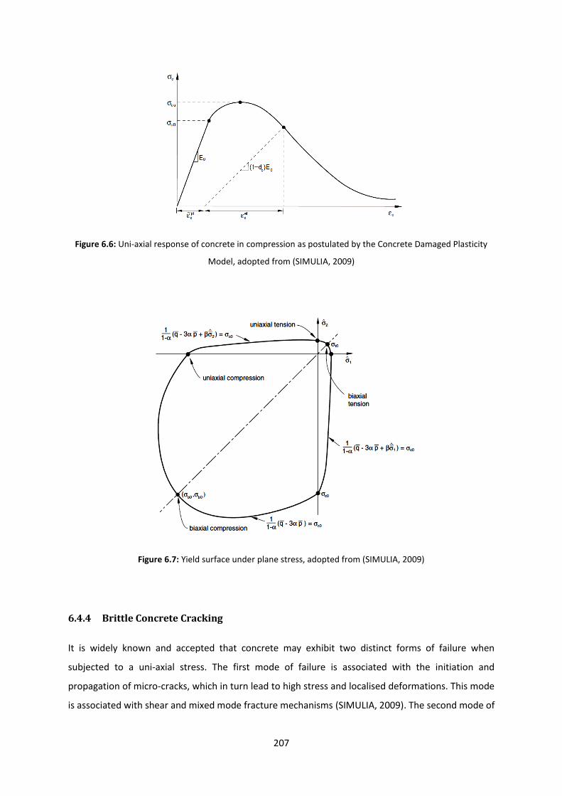
207
Figure 6.6: Uni-axial response of concrete in compression as postulated by the Concrete Damaged Plasticity
Model, adopted from (SIMULIA, 2009)
Figure 6.7: Yield surface under plane stress, adopted from (SIMULIA, 2009)
6.4.4 Brittle Concrete Cracking
It is widely known and accepted that concrete may exhibit two distinct forms of failure when
subjected to a uni-axial stress. The first mode of failure is associated with the initiation and
propagation of micro-cracks, which in turn lead to high stress and localised deformations. This mode
is associated with shear and mixed mode fracture mechanisms (SIMULIA, 2009). The second mode of

208
failure is one where micro and macro-cracking develop evenly around the specimen, thus leading to
uniform deformations. This mode is mainly associated with ‘distributed micro-cracking mechanisms
that are primarily observed under compression states of stress’ (SIMULIA, 2009). The first mode of
failure is strongly associated with the tension softening behaviour of concrete, whereas the second
is more characteristic of its compression response. The brittle concrete cracking model incorporated
in ABAQUS, and described herein deals with the first mode of failure.
The concrete brittle cracking model can be classified as a ‘smeared cracking model’. This is
essentially due to the fact that the individual macro-cracks are not modelled discretely. The
presence of cracking is however taken into account in the stress and material stiffness matrices at
each integration point.
The crack detection in this model obeys a simple Rankine criterion. According to this criterion, crack
formation occurs when the principal tensile stress exceeds that tensile strength of the specimen. The
Rankine criterion in the deviatoric plane as well as in the state of plane stress is shown in Figures 6.8
and 6.9, respectively.
Figure 6.8: Rankine criterion in the deviatoric plane, as adopted from (SIMULIA, 2009)
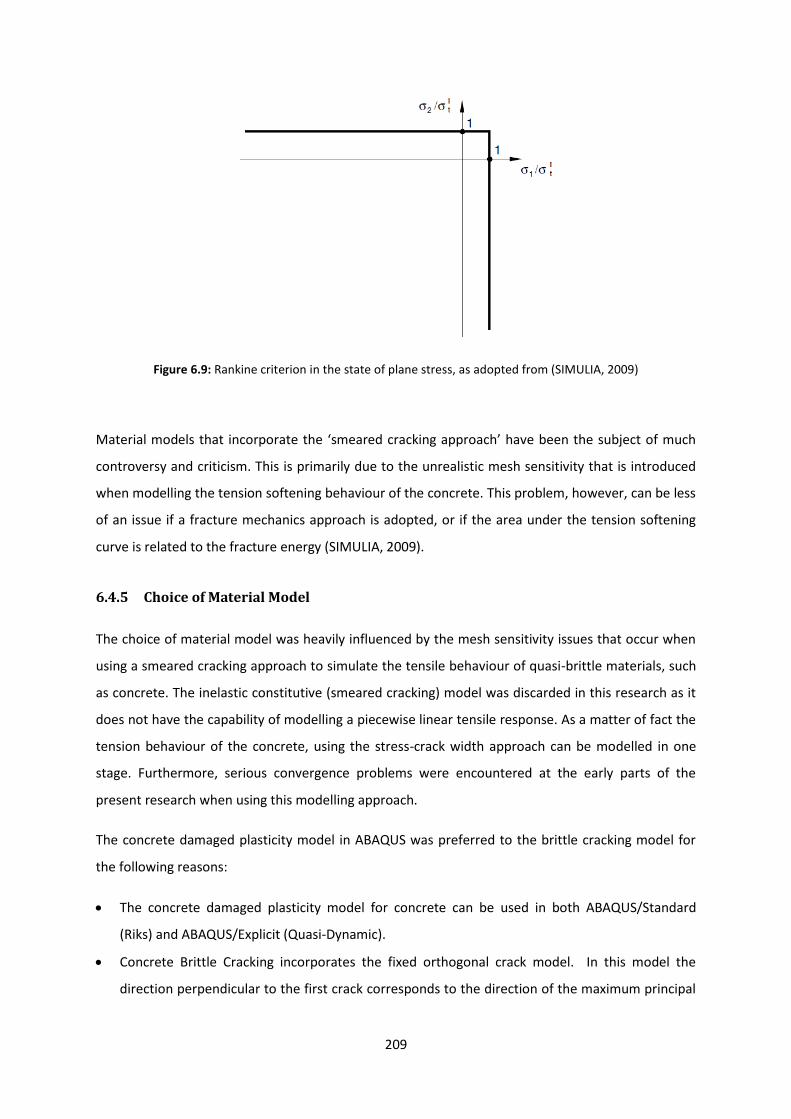
209
Figure 6.9: Rankine criterion in the state of plane stress, as adopted from (SIMULIA, 2009)
Material models that incorporate the ‘smeared cracking approach’ have been the subject of much
controversy and criticism. This is primarily due to the unrealistic mesh sensitivity that is introduced
when modelling the tension softening behaviour of the concrete. This problem, however, can be less
of an issue if a fracture mechanics approach is adopted, or if the area under the tension softening
curve is related to the fracture energy (SIMULIA, 2009).
6.4.5 Choice of Material Model
The choice of material model was heavily influenced by the mesh sensitivity issues that occur when
using a smeared cracking approach to simulate the tensile behaviour of quasi-brittle materials, such
as concrete. The inelastic constitutive (smeared cracking) model was discarded in this research as it
does not have the capability of modelling a piecewise linear tensile response. As a matter of fact the
tension behaviour of the concrete, using the stress-crack width approach can be modelled in one
stage. Furthermore, serious convergence problems were encountered at the early parts of the
present research when using this modelling approach.
The concrete damaged plasticity model in ABAQUS was preferred to the brittle cracking model for
the following reasons:
The concrete damaged plasticity model for concrete can be used in both ABAQUS/Standard
(Riks) and ABAQUS/Explicit (Quasi-Dynamic).
Concrete Brittle Cracking incorporates the fixed orthogonal crack model. In this model the
direction perpendicular to the first crack corresponds to the direction of the maximum principal

210
tensile stress. The direction of the first crack is taken into account in the subsequent
calculations, by allowing crack formations in orthogonal directions to this crack. A number of
objections have been raised against the use of models incorporating fixed orthogonal cracks. The
incorporation of shear retention tends to make the model too stiff (SIMULIA, 2009). Such
behaviour was observed during the modelling of the three-point bending beam tests, as
described in the subsequent sections of the present report.
The brittle cracking philosophy does not take into account the plastic characteristics of concrete
under compression. As a matter of fact, concrete is assumed to act in a linear elastic fashion.
Although this is a reasonable assumption in the case of the three point bending beam tests, the
model can prove to be quite restrictive.
Furthermore, during the preliminary part of the present research it was found that when
modelling notched beam tests, the strain pattern exhibited using the Concrete Damaged
Plasticity corresponds more closely to the actual experimental behaviour.
6.5 Constitutive Model Adopted
6.5.1 Introductory Principles
Concrete can be classified as a quasi-brittle material, exhibiting behaviour identical or similar to
different rock types or ceramics. Similarly to these quasi-brittle materials, there are two main causes
that can give rise to failure; crushing when subjected to severe compressive stress and cracking
when subjected to tensile loads.
As a result different stiffness effects, as well as ‘different degradation of the elastic stiffness’
(SIMULIA, 2009) can be observed in tension and compression. This can also be extended to include
the stiffness recovery effects under dynamic or cyclic loading. However, such a discussion is beyond
the scope of this chapter.
Lubliner at al. (1989) and Lee and Fenves (1998) used the above axioms to create constitutive
models for concrete taking into account the degradation of the elastic stiffness. These models form
the foundation upon which the Concrete Damaged Plasticity Model native to ABAQUS, and adopted
in the current study, is based.
All the figures and information presented in the following subsections have been extracted from the
relevant ABAQUS 6.9.1 documentation.
211
6.5.2 Uni-axial tension and compression conditions
The adopted concrete damaged plasticity model assumes that both the uni-axial tension and
compression responses are governed by the damaged plasticity rule, as illustrated in Figures 6.4 and
6.5. For the case of uniaxial tension, concrete is assumed to behave in a linear elastic fashion until a
stress, 0t has been reached (SIMULIA, 2009). This stress determines the start of micro-cracking in
the concrete matrix. The behaviour beyond this point is characterised by a tension softening
response thus making it suitable for the modelling of structures with low fibre dosages.
In a similar manner, when subjected to uniaxial compression the model behaves in a linear elastic
fashion until a compressive yield stress, 0c has been reached. After this point, some strain
hardening may be observed until the ultimate compressive stress cu is reached. Beyond this point, a
softening response is assumed by the model (SIMULIA, 2009).
When the structure in question is unloaded in the strain softening part of the curve, a permanent
plastic deformation occurs. As a result the response of the material, should it be loaded
subsequently, is considerably weaker due to the damage caused by the plastic deformation. The
‘degradation of stiffness’ is characterised by the following two variables, td and cd , which the
present model assumes them to be defined as functions of the plastic strain, the temperature or
other field variables (SIMULIA, 2009).
10;,, ti
t
plt dffd (6.16)
10;,, ti
t
plt dffd (6.17)
A degradation of stiffness coefficient of zero indicates an undamaged specimen. On the other hand,
a degradation stiffness coefficient of one represents a specimen that is fully damaged and suffers a
complete loss of its strength.
Subsequently, the following expressions can be derived to describe the behaviour of concrete under
uniaxial tension and compression conditions, assuming an undamaged specimen:
pltttt Ed 01 (6.18)
plcccc Ed 01 (6.19)

212
where, 0E represents the elastic stiffness matrix of a specimen without any damage. The effective
cohesive stresses for tension and compression can then be defined as follows: These stresses
determine the size of the yield surface, illustrated in Figure 6.6:
pltt
t
t
t Ed
01
(6.20)
plcc
c
c
c Ed
01
(6.21)
The same principles can be extended to cover the cases for dynamic and cyclic loading, where the
presence of the degradation coefficients is of higher importance. However, such a discussion is
beyond the scope of this chapter. For a more detailed discussion of the constitutive equations
applied and, indeed, the application of this model in the FEM the interested reader is referred to the
research by Lubliner at al. (1989) and Lee and Fenves (1998) and the ABAQUS 6.9.1 Theory and
User’s Manuals.
6.5.3 Post-Failure Tensile behaviour
The post-failure tensile response of concrete can be usually defined in terms of its cracking strain
(SIMULIA, 2009). The cracking strain c is defined as the total strain t minus the elastic strain el .
eltc (6.22)
The elastic strain may be defined as:
0Eel
(6.23)
where, denotes the tensile stress and 0E denotes the ‘undamaged’ elastic modulus of the
specimen in question.
The present discussion can be extended to cover the quantifying of the damage invoked by cyclic
and dynamic modelling on the tensile behaviour of the concrete. However, this is beyond the scope
of the present investigation. The interested reader is referred to the ABAQUS 6.9.1 Theory and User
Manuals where a more detailed explanation of the underlying principles takes place.
Defining stress as a function of the total strain (using a stress – strain response without considering
fracture energy) can introduce unreasonable mesh sensitivities to scenarios where little, or as in the
213
present case, no additional reinforcement is incorporated (SIMULIA, 2009). This is due to the fact
that the calculations of the Finite Element Method (FEM) do not ‘converge to a unique solution’
(SIMULIA, 2009). In the case of the SFRC refining the mesh may lead to narrower crack widths
(Pilakoutas, Neocleous, & Guadagnini, 2002), particularly if localised failure occurs, as for instance in
the case of a beam under three-point bending. The fibre content used in the present research gives
rise to a tension softening response, which can additionally cause convergence difficulties, as
illustrated earlier in the present chapter. In many cases, the incorporation of tension reinforcement
or the introduction of additional tension stiffening can eliminate the problem and thus a stress-
strain response can be used.
In such cases a stress – displacement response, or w as it is more commonly referred to, is more
suitable for use in the NLFEA. The Hillerborg energy fracture criterion is adopted within ABAQUS,
which enables the user to define the post-cracking failure response in terms of the crack width
(Hillerborg et al., 1976) (RILEM Technical Committee, 2002). The initial constitutive model developed
by Hillerborg et al. (1976) as well as its application to the SFRC (Hillerborg, 1980) has been described
and discussed in section 2.5.2 of the present research thesis. Within the framework of the Concrete
Damaged Plasticity Model, the post-failure response can be specified in terms of a stress-strain
relationship that is related to the fracture energy. Although, this method adopts all the advantages
offered by the σ-w approach it assumed that the post failure response is linear, which provides
substantial restrictions in the modelling of the SFRC. For the reasons discussed above the w
approach was adopted for the FE modelling.
6.5.4 Post-Failure Compressive behaviour
The compressive behaviour assumed by the current model is illustrated in Figure 6.5. The
compressive stress is defined as a function of the compressive strain (SIMULIA, 2009). ABAQUS uses
the inelastic strain,
in
c rather than the plastic strain pl
c . The inelastic strain is defined as follows:
el
c
t
c
in
c (6.24)
where, pl
c denotes the total strain. The elastic strain,
el
c can be accordingly defined as follows:
0E
cel
c
(6.25)
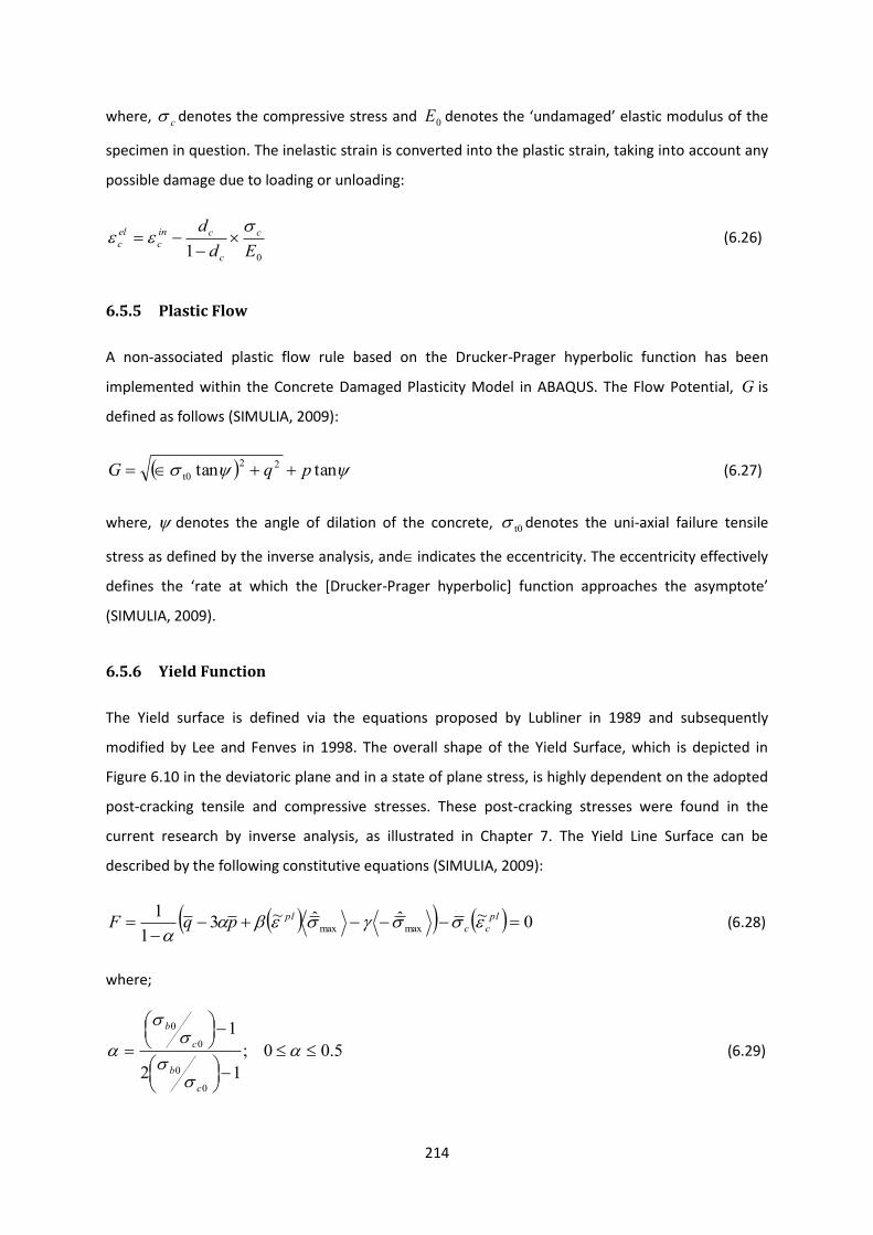
214
where, c denotes the compressive stress and 0E denotes the ‘undamaged’ elastic modulus of the
specimen in question. The inelastic strain is converted into the plastic strain, taking into account any
possible damage due to loading or unloading:
01 Ed
d c
c
cin
c
el
c
(6.26)
6.5.5 Plastic Flow
A non-associated plastic flow rule based on the Drucker-Prager hyperbolic function has been
implemented within the Concrete Damaged Plasticity Model in ABAQUS. The Flow Potential, G is
defined as follows (SIMULIA, 2009):
tantan 22
t0 pqG (6.27)
where, denotes the angle of dilation of the concrete, t0 denotes the uni-axial failure tensile
stress as defined by the inverse analysis, and indicates the eccentricity. The eccentricity effectively
defines the ‘rate at which the *Drucker-Prager hyperbolic+ function approaches the asymptote’
(SIMULIA, 2009).
6.5.6 Yield Function
The Yield surface is defined via the equations proposed by Lubliner in 1989 and subsequently
modified by Lee and Fenves in 1998. The overall shape of the Yield Surface, which is depicted in
Figure 6.10 in the deviatoric plane and in a state of plane stress, is highly dependent on the adopted
post-cracking tensile and compressive stresses. These post-cracking stresses were found in the
current research by inverse analysis, as illustrated in Chapter 7. The Yield Line Surface can be
described by the following constitutive equations (SIMULIA, 2009):
0~ˆˆ~31
1maxmax
pl
cc
plpqF
(6.28)
where;
5.00;
12
1
0
0
0
0
c
b
c
b
(6.29)
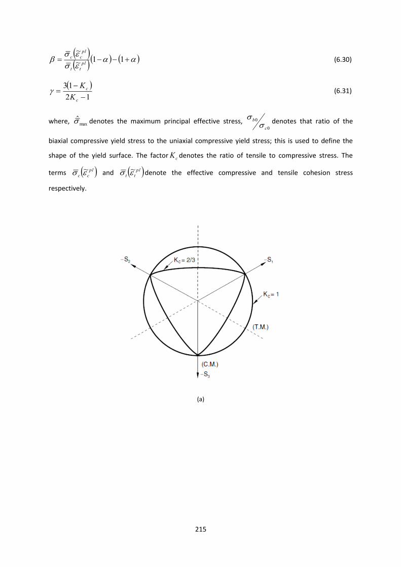
215
11~
~
pl
tt
pl
cc (6.30)
12
13
c
c
K
K (6.31)
where, max̂ denotes the maximum principal effective stress, 0
0
c
b
denotes that ratio of the
biaxial compressive yield stress to the uniaxial compressive yield stress; this is used to define the
shape of the yield surface. The factor cK denotes the ratio of tensile to compressive stress. The
terms plcc ~ and pltt ~ denote the effective compressive and tensile cohesion stress
respectively.
(a)

216
(b)
Figure 6.10: Yield surfaces in (a) the deviatoric plane corresponding to different values of K and (b) in a state of
plane stress
6.6 Material Parameters used in Damaged Plasticity Model
6.6.1 General Remarks
As described in the preceding subsections, a number of material parameters need to be defined by
the user to configure the concrete damaged plasticity model. The parameters described within the
context of the present section have been used throughout this investigation.
6.6.2 Poisson’s ratio
The Poisson’s ratio is the ratio of the expansion or contraction that occurs in the transverse direction
as a result of a compressive or tensile load. For uncracked concrete materials, the Poisson ratio
tends to vary between 0.15 – 0.20 (Illston & Domone, 2004). As the variability of this parameter is
sufficiently small, it can be deemed insignificant to influence the NLFEA results (Abbas, 2002) (Labib,
2008). Referring to previous work in the analysis of the SFRC (Labib, 2008), a value of 0.2 has also
been adopted in the present study.

217
6.6.3 Elastic (Young’s) Modulus
Previous research has demonstrated a small but insignificant decrease in Young’s Modulus after the
addition of the steel fibres to the concrete matrix (Neves et al., 2005). The empirical formulae used
by the relevant standards can determine with reasonable accuracy the Young’s Modulus. The
average compressive strength of the cubes (reinforced with steel fibres) has been used in the
calculation of the Young’s Modulus.
6.6.4 Uniaxial Compressive Behaviour
The uniaxial compressive behaviour does not play a significant part in the analysis and design of pile-
supported slabs, as the failure occurs at the tension face of the structure. Furthermore, significant
cracking occurs before any concrete yielding (due to compression) takes place.
The failure stress under compression has been extracted from the results of the cube compressive
tests undertaken. A small sensitivity analysis was undertaken during the early stages of the research
which demonstrated the low sensitivity of this parameter in the adopted model.
6.6.5 Uniaxial Tensile Behaviour
The uniaxial tensile stress – displacement response is one of the most dominant parameters that
affect the performance of the model. The uniaxial tensile behaviour of the SFRC has been derived
using the inverse method on the notched beam test results. This method is described in Chapter 7 of
the present thesis.
6.6.6 Plastic Flow
The plastic flow of concrete, as dictated by equation 6.27, is determined by the angle of dilation of
concrete as well as the eccentricity. The eccentricity determines the ‘rate at which the *plastic flow+
function approaches the asymptote’ (SIMULIA, 2009).
The angle of dilation of concrete has been the subject of previous research. Previous work relating to
the present field adopted an angle of dilation of 10° (Labib, 2008) (Marinkovic & Alendar, 2008).
Marinkovic et al. (2008) used a dilation angle of 10° in their numerical model simulating the
punching failure of reinforced concrete slabs. Labib (2008) used the same value in the analysis of
SFRC ground suspended floor slabs under punching shear. The same value has been used herein in
accordance with previous research. The default value for the eccentricity is 0.1. A value of 0.1 would
218
make the plastic flow potential relatively insensitive to variations in the angle of dilation.
Consequently, a value of 0.1 has been used.
6.6.7 Ratio of Biaxial to Uniaxial Compressive Strength
The ratio of biaxial to uniaxial compressive strength effectively determines the shape and size of the
failure surface of the SFRC in compression. The most reliable test results in regard to this parameter
where undertaken by Kupfer et al. in 1969. The ratio of the biaxial to the uniaxial strength of
concrete based on Kupfer’s work was derived as 1.16. This value was subsequently adopted by
Kmiecik et al. (2011) in an attempt to identify and configure the parameters of the concrete damage
plasticity model.
The default value used in ABAQUS is 1.16 (SIMULIA, 2009) following the work of Kupfer et al. (1969)
and this is the value that has been adopted for the present research. Lastly, the ratio of the second
stress invariant on the tensile meridian to that of the compressive meridian, cK has been assumed
to be 2/3. This is in accordance with SIMULIA (2009) as well as with previous work undertaken by
Jankowiac et al. (2005), Labib (2008) and Kmiecik at al. (2011).
6.7 Concluding Remarks
The intention of this chapter was to give the interested reader an insight into the NLFEA models
used in this thesis. A brief overview of the basic principles of the discrete and smeared crack
modelling approaches was given.
An introduction of the foundation principles of the finite element method was presented along with
an explanation in its applications in concrete modelling. This was followed by a discussion of the
concrete damaged plasticity, brittle and smeared cracking constitutive models available in ABAQUS
with particular focus on the philosophy of each.
The concrete damage plasticity model was considered as the most viable option due to the
constraints of the brittle and smeared cracking models discussed. The philosophy of this model was
discussed along with the material parameters used. The material parameters were determined
based on recommendations of previous researchers as well as preliminary sensitivity analysis
undertaken by the author. The present chapter has provided a number of useful recommendations
in the NLFEA undertaken in the chapters that follow.
219
Chapter Seven
Numerical Modelling of Structural Tests
7.1 General Remarks
The literature review in Chapter Three describes various standardised structural tests which are
routinely used to determine the material properties of SFRC. It also outlines the advantages and
disadvantages of each method. As discussed in Chapter Three, there is a lack of consensus amongst
researchers and manufacturers over which test is most appropriate. This causes confusion amongst
designers as well as deterring them from using SFRC in cases where its use would be beneficial.
This chapter presents the results of the numerical analyses undertaken to simulate the structural
tests described in Chapter Three. Section 7.2 describes the inverse analysis that was used to
determine the relationship between stress and crack width in the notched beam tests. Sections 7.3
and 7.4 describe the numerical model and numerical results for the RDP. Section 7.5 outlines the
smeared crack inverse analysis used on the RDP whereas section 7.6 presents the numerical results
of two span slabs.
7.2 Inverse Analysis of Notched Beam Tests using Discrete Cracking
7.2.1 General Overview
The inverse analysis method involves ‘back calculating’ a stress – crack width (σ-w) response based
on previous experimental data. It is a process of reverse engineering to get from the structural
response to the intrinsic material properties. The introduction of the NLFEA and the use of
computers have made this process relatively straightforward to carry out. Figure 7.1 illustrates the
main stages of the inverse analysis procedure, as adopted from Kooiman (2000). This process can be
subdivided into four stages. The first stage involves the input of the initial values. A small parametric
study could be undertaken to establish which variables affect the structural behaviour and have to
be determined by inverse analysis. The assumptions regarding the type of response have to be made
at this stage, whether it is linear, bi-linear etc.

220
Input Values
NLFEA Adjusted values
Experiment = NLFEA ?
Final values
Figure 7.1: Inverse analysis procedure followed in the present investigation (adapted from (Kooiman, 2000)
0
5
10
15
0 2 4 6 8
Load
(kN
)
Displacement (mm)
Experiment
NLFEA
No
Yes
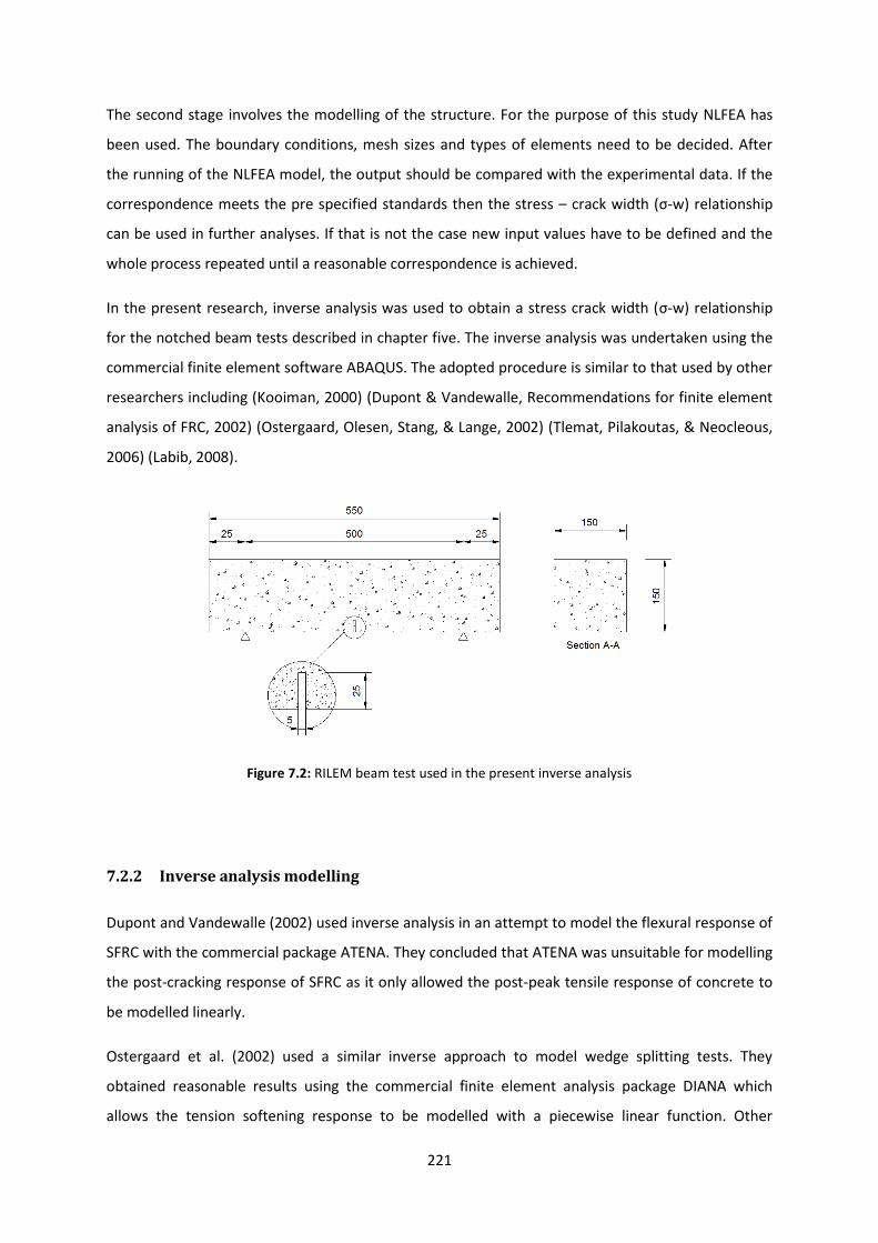
221
The second stage involves the modelling of the structure. For the purpose of this study NLFEA has
been used. The boundary conditions, mesh sizes and types of elements need to be decided. After
the running of the NLFEA model, the output should be compared with the experimental data. If the
correspondence meets the pre specified standards then the stress – crack width (σ-w) relationship
can be used in further analyses. If that is not the case new input values have to be defined and the
whole process repeated until a reasonable correspondence is achieved.
In the present research, inverse analysis was used to obtain a stress crack width (σ-w) relationship
for the notched beam tests described in chapter five. The inverse analysis was undertaken using the
commercial finite element software ABAQUS. The adopted procedure is similar to that used by other
researchers including (Kooiman, 2000) (Dupont & Vandewalle, Recommendations for finite element
analysis of FRC, 2002) (Ostergaard, Olesen, Stang, & Lange, 2002) (Tlemat, Pilakoutas, & Neocleous,
2006) (Labib, 2008).
Figure 7.2: RILEM beam test used in the present inverse analysis
7.2.2 Inverse analysis modelling
Dupont and Vandewalle (2002) used inverse analysis in an attempt to model the flexural response of
SFRC with the commercial package ATENA. They concluded that ATENA was unsuitable for modelling
the post-cracking response of SFRC as it only allowed the post-peak tensile response of concrete to
be modelled linearly.
Ostergaard et al. (2002) used a similar inverse approach to model wedge splitting tests. They
obtained reasonable results using the commercial finite element analysis package DIANA which
allows the tension softening response to be modelled with a piecewise linear function. Other

222
researchers have also used bilinear σ-w relationships to obtain reasonable agreement with
experimental data (Ostergaard, Olesen, Stang, & Lange, 2002) (Tlemat, Pilakoutas, & Neocleous,
2006). Stang (2002) used an alternative approach to model discrete cracks in DIANA. He modelled
the σ-w response using non-linear springs placed between the nodes (Stang, 2002). Hemmy (2002)
used analysis for the modelling of SFRC under three-point loading using ANSYS. However, he was
constrained by the fact that ANSYS only allows materials with a tension softening response to be
modelled using a linear response. Tlemat et al. (2006) successfully used ABAQUS to perform an
inverse analysis of the RILEM notched beam test. They used a four segment piecewise linear in
conjunction with an element size of 25mm. Labib (2008) also used ABAQUS to perform an inverse
analysis of the RILEM notched beam test. The inverse method yielded a constitutive model which
was used in subsequent analyses (Labib, 2008).
7.2.3 Input Parameters
The main parameters that influence the load-deflection response of a beam in three point bending
(Figure 7.2) are the stress – crack width relation σ-w (under direct tension) and the concrete elastic
modulus. As the EN 14651 beam test fails in flexural tension, the concrete compressive strength, and
the shape of the assumed stress-strain curve in compression, adopted in the analysis has little effect
on the calculated response (Labib, 2008). Sensitivity studies by the author confirmed this. The
present NLFEA adopts a stress – crack width (σ-w) relationship rather than a stress –strain (σ-ε) one.
The bi-linear σ-w relationship shown in Figure 7.3 is used in the present study, as it was found to be
the simplest relationship capable of modelling the observed responses of the notched beams by the
author.
Figure 7.3: Tension softening response assumed for the inverse analysis procedure
223
7.2.4 Non Linear Finite Element Analysis (NLFEA)
The beam illustrated in Figure 7.2 was modelled using a ‘pseudo-discrete’ cracking approach. The
beam was modelled with shell elements using the mesh shown in Figure 7.6a and with plane stress
elements using the mesh shown in Figure 7.6b. In each case, the elements at the crack were
modelled as nonlinear with the element to either side modelled elastically. In Figure 7.6(a), the
elements at the crack were modelled using the four-noded shell element S4R (Figure 7.4(a)) whereas
the elements to either side of the crack were modelled using the three-noded shell element S3R
(Figure 7.4(b)). Shell elements were used as in-plane bending stresses are dominant. Nine Gauss
points were defined through the thickness of the beam as preliminary analyses done by the author
showed that using more Gauss points does not improve accuracy significantly (Figure 7.5). The
reduced integration option was enabled to prevent shear locking.
The depth of the section was defined as the depth of the beam minus the height of the notch.
Preliminary FE runs showed that the load-deflection response of the beam is not influenced
significantly by the concrete below the notch. The mesh adopted is shown in Figure 7.6 (a). An
element size of 20mm was used. Choosing too small a mesh size results in very large strains when
the crack width exceeds the element size whereas choosing a too large a mesh size leads to
inaccurate solutions.
The load deflection response was found to vary considerably with the element size for a given σ-w
relationship as shown in Figure 7.7 for elements less than 20mm due to geometric non linearities.
Geometric non linearities became significant, as the crack width approached the element size, due
to the plastic strains becoming large compared to the element size. The final mesh size was chosen
after a systematic investigation into the influence of element size on the calculated response.
Choosing too small a mesh size is undesirable as it results in very large strains when the crack width
exceeds the element size. This in turn causes a loss of objectivity due to the influence of geometric
nonlinearities on the assumed -w relationship. On the other hand choosing a too large mesh size
leads to inaccurate solutions. A quasi-static analysis was used ensuring the load is applied sufficiently
slowly to ensure dynamic effects were negligible.
A comparative analysis of the notched beam was also carried out using plane stress elements (Figure
7.6(b)). The elements above the notch were modelled using four noded plane stress elements with
reduced integration. The ‘elastic’ region either side of the crack, was done using three-noded
triangular elements. Figure 7.8 compares the measured and predicted load displacement responses
for castings C1 to C4 obtained using the σ-w responses shown in Figure 7.9 for shell elements. The
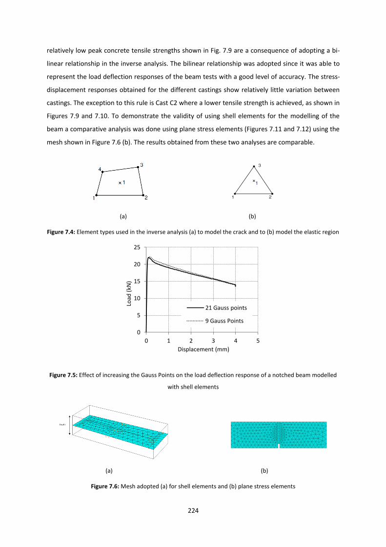
224
relatively low peak concrete tensile strengths shown in Fig. 7.9 are a consequence of adopting a bi-
linear relationship in the inverse analysis. The bilinear relationship was adopted since it was able to
represent the load deflection responses of the beam tests with a good level of accuracy. The stress-
displacement responses obtained for the different castings show relatively little variation between
castings. The exception to this rule is Cast C2 where a lower tensile strength is achieved, as shown in
Figures 7.9 and 7.10. To demonstrate the validity of using shell elements for the modelling of the
beam a comparative analysis was done using plane stress elements (Figures 7.11 and 7.12) using the
mesh shown in Figure 7.6 (b). The results obtained from these two analyses are comparable.
(a) (b)
Figure 7.4: Element types used in the inverse analysis (a) to model the crack and to (b) model the elastic region
Figure 7.5: Effect of increasing the Gauss Points on the load deflection response of a notched beam modelled
with shell elements
(a) (b)
Figure 7.6: Mesh adopted (a) for shell elements and (b) plane stress elements
0
5
10
15
20
25
0 1 2 3 4 5
Load
(kN
)
Displacement (mm)
21 Gauss points
9 Gauss Points
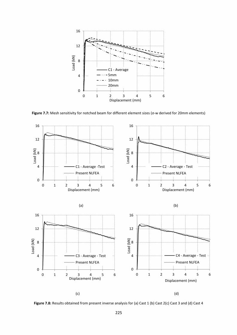
225
Figure 7.7: Mesh sensitivity for notched beam for different element sizes (σ-w derived for 20mm elements)
(a) (b)
(c) (d)
Figure 7.8: Results obtained from present inverse analysis for (a) Cast 1 (b) Cast 2(c) Cast 3 and (d) Cast 4
0
4
8
12
16
0 1 2 3 4 5 6
Load
(kN
)
Displacement (mm)
C1 - Average
5mm
10mm
20mm
0
4
8
12
16
0 1 2 3 4 5 6
Load
(kN
)
Displacement (mm)
C1 - Average -Test
Present NLFEA
0
4
8
12
16
0 1 2 3 4 5 6
Load
(kN
)
Displacement (mm)
C2 - Average - Test
Present NLFEA
0
4
8
12
16
0 1 2 3 4 5 6
Load
(kN
)
Displacement (mm)
C4 - Average - Test
Present NLFEA
0
4
8
12
16
0 1 2 3 4 5 6
Load
(kN
)
Displacement (mm)
C3 - Average - Test
Present NLFEA
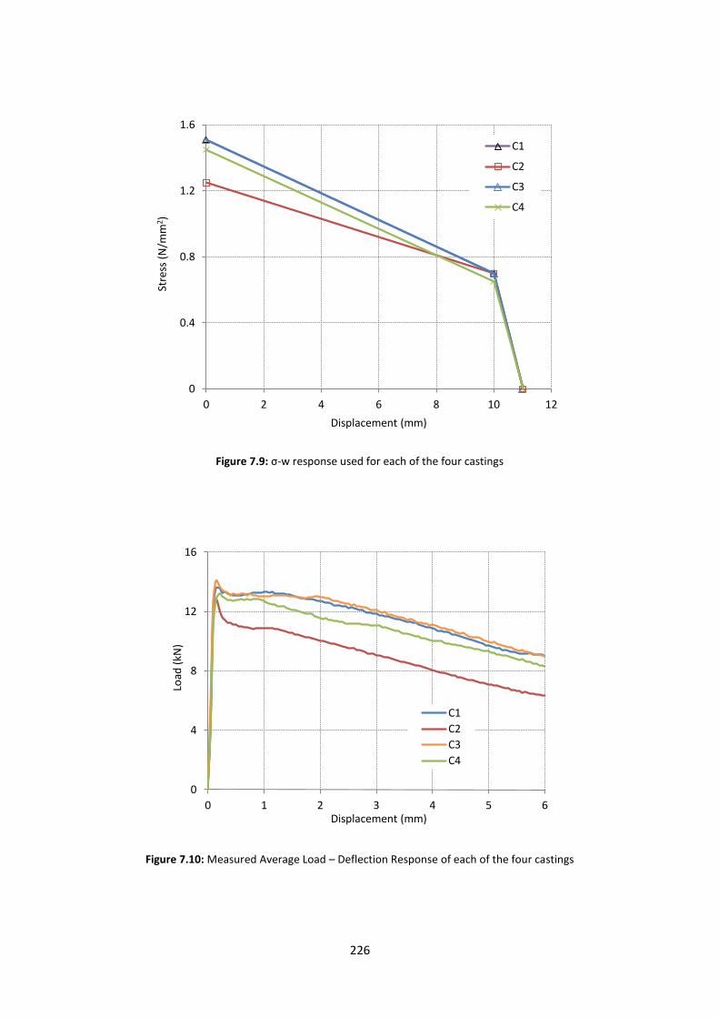
226
Figure 7.9: σ-w response used for each of the four castings
Figure 7.10: Measured Average Load – Deflection Response of each of the four castings
0
0.4
0.8
1.2
1.6
0 2 4 6 8 10 12
Stre
ss (
N/m
m2 )
Displacement (mm)
C1
C2
C3
C4
0
4
8
12
16
0 1 2 3 4 5 6
Load
(kN
)
Displacement (mm)
C1
C2
C3
C4
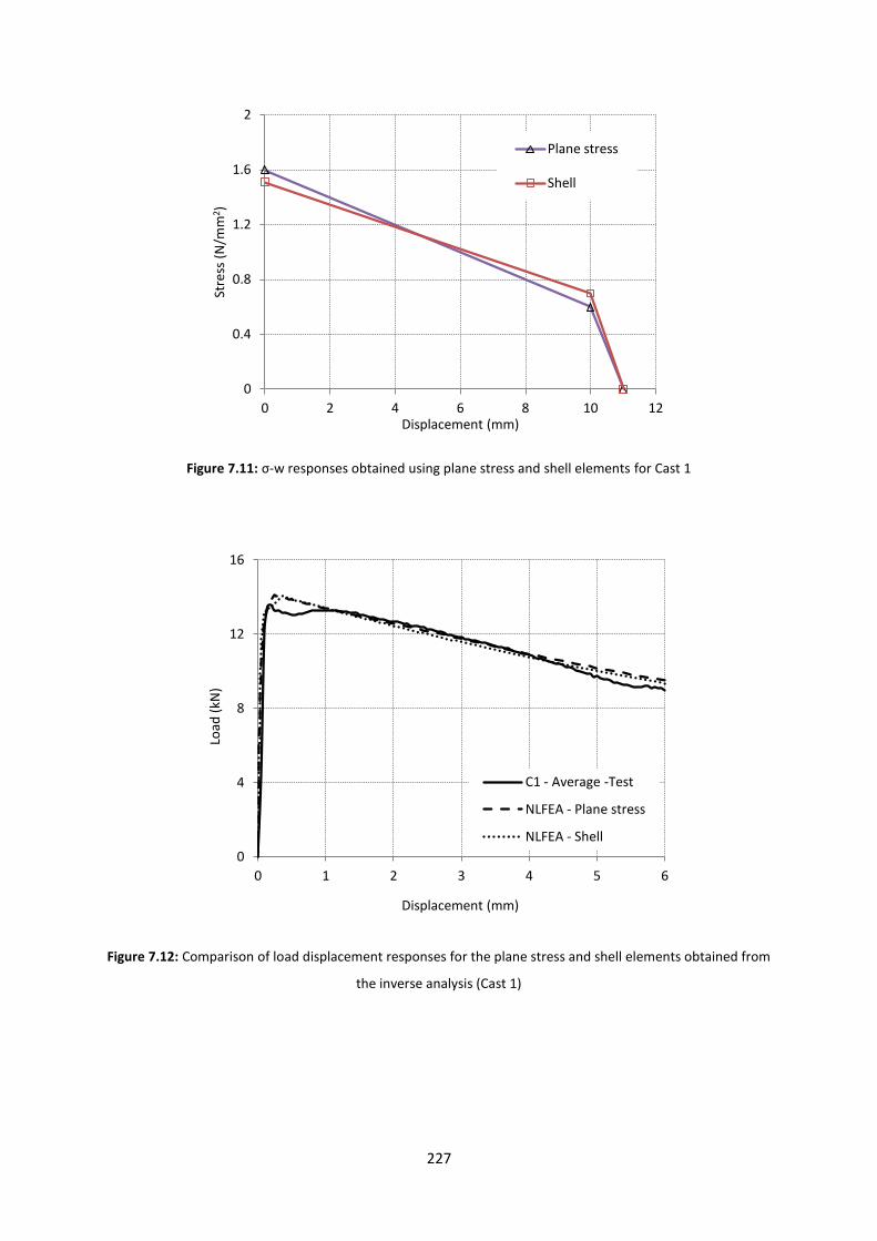
227
Figure 7.11: σ-w responses obtained using plane stress and shell elements for Cast 1
Figure 7.12: Comparison of load displacement responses for the plane stress and shell elements obtained from
the inverse analysis (Cast 1)
0
0.4
0.8
1.2
1.6
2
0 2 4 6 8 10 12
Stre
ss (
N/m
m2 )
Displacement (mm)
Plane stress
Shell
0
4
8
12
16
0 1 2 3 4 5 6
Load
(kN
)
Displacement (mm)
C1 - Average -Test
NLFEA - Plane stress
NLFEA - Shell

228
7.3 Analysis of Round Determinate Plate
7.3.1 Introduction to Yield Line Analysis
The Round Determinate Plate (RDP) Tests were initially modelled with classical yield line analysis
(Johansen, 1972), in which the rotations, and hence moments, are assumed to be constant along the
yield lines. This assumption is valid for concrete structures reinforced with conventional
reinforcement but it is only an approximation for SFRC slabs near their peak load when the crack
width varies along its length as demonstrated experimentally in Chapter Five.
7.3.2 Yield Line Analysis of Statically Determinate Round Panel
The arrangement adopted for the statically determinate plate test is replicated below for
convenience (Figure 7.13): The plate thickness was chosen to the same as that above the notch in
the beam tests to minimise size effects.
Figure 7.13: Test arrangement adopted for the statically determinate round panel test
Using the fundamental principle of the Yield Line Theory:
External work done by the loads = Internal Energy dissipated in the yield lines
extU P (7.1)

229
where, P denotes and load and the vertical displacement.
int 3 3U Rm (7.2)
where, R denotes the radius of the specimen, the rotation relative to the supports andm is the
moment along each yield line per unit length. Projecting the yield line onto the pivot line:
3x r (7.3)
where, r is the radius of the plate to the supports.
The rotation in the yield lines is given by:
3 (7.4)
r
(7.5)
Figure 7.14: Yield and pivot boundaries of a round panel specimen analysed with Yield Line Theory (Bernard,
2005).
Therefore calculating the internal energy we obtain:
rRm
r
rPU i 331int
(7.6)

230
The load, P is given by the following equation:
3 3
i
RP m
r r
(7.7)
R denotes the radius of the RDP (500mm), r is the radius to the supports (475mm) and ir is the
radius of the loading plate (50mm). The moments from the notched beam tests can be used in
Equation 7.7 in order to estimate the failure load of the RDP.
The crack width can be estimated by multiplying the rotation in the yield line by the depth of the
round panel:
46.0475
12533 h
rw
(7.8)
7.4 Comparative Analysis of RDP with NLFEA and Yield Line Analysis
7.4.1 Input Parameters
This section uses NLFEA to investigate the realism of the simplifying assumptions made in the Yield
Line analysis of RDP, as described in Section 3.4. The pseudo discrete crack approach is used for the
NLFEA in this section.
The load has been defined as a line load around the perimeter of the loading plate as the contact
area moves towards the perimeter of the loading plate during the test. It also avoids the problem of
unrealistic behaviour being predicted as a result of very large stresses developing in the central
element of the plate. Modelling the loading plate using such an approach seems also to be the most
realistic alternative to defining a contact model with the added advantage of being a
computationally cheaper solution.
A NLFEA was carried out using the finite element mesh shown in Figure 7.15 in which the cracking
was localised within elements of width 20mm as in the modelling of the notched beam tests (Figure
7.16). To model the cracks, four-noded rectangular shell elements were used with reduced
integration (S4R) (Figure 7.4(a)). For the modelling of the ‘elastic’ region three-noded triangular
elements with reduced integration were used (Figure 7.4(b)). The analyses were carried out using
the σ-w relationship derived for Cast 1 of the notched beams in Figure 7.8. The tensile strength of

231
the elements outside the predetermined crack locations was increased to ensure that cracking was
largely confined to the predetermined zones.
Figure 7.15: Mesh adopted for present case study
Figure 7.16: Crack pattern observed for the Round Determinate Round Panel Test
7.4.2 Results of analysis of RDP tests
Figure 7.17 shows that the results from the NLFEA and the yield line analysis using the average
notched beam test results show considerable differences in the load deflection behaviour. The yield
line resistance,P was calculated as a function of the central displacement using equation 7.7 in
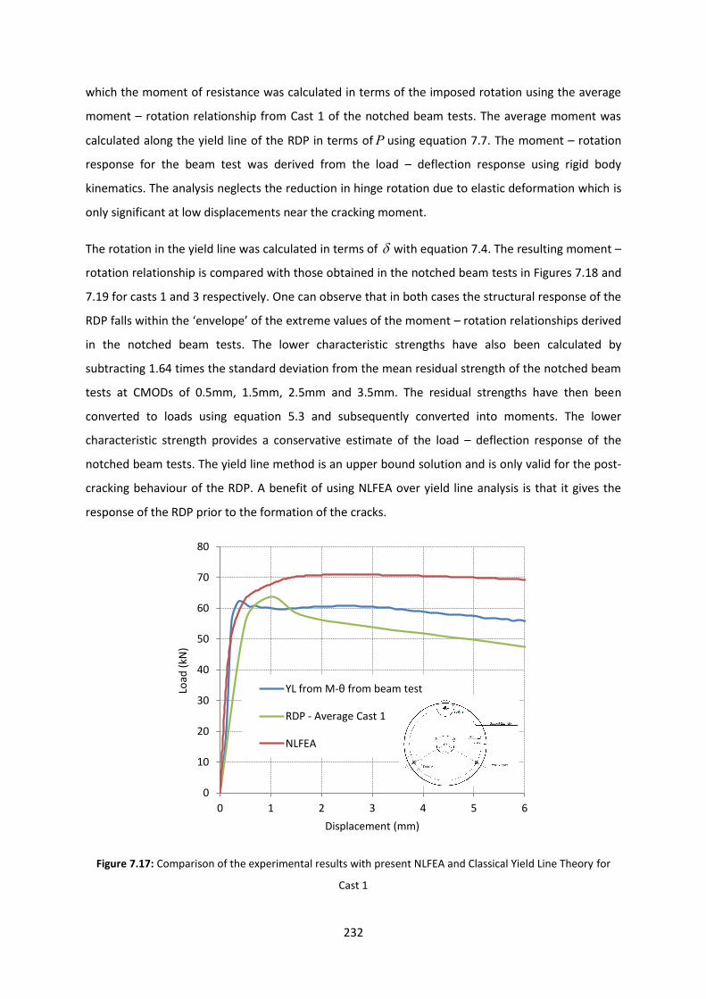
232
which the moment of resistance was calculated in terms of the imposed rotation using the average
moment – rotation relationship from Cast 1 of the notched beam tests. The average moment was
calculated along the yield line of the RDP in terms ofP using equation 7.7. The moment – rotation
response for the beam test was derived from the load – deflection response using rigid body
kinematics. The analysis neglects the reduction in hinge rotation due to elastic deformation which is
only significant at low displacements near the cracking moment.
The rotation in the yield line was calculated in terms of with equation 7.4. The resulting moment –
rotation relationship is compared with those obtained in the notched beam tests in Figures 7.18 and
7.19 for casts 1 and 3 respectively. One can observe that in both cases the structural response of the
RDP falls within the ‘envelope’ of the extreme values of the moment – rotation relationships derived
in the notched beam tests. The lower characteristic strengths have also been calculated by
subtracting 1.64 times the standard deviation from the mean residual strength of the notched beam
tests at CMODs of 0.5mm, 1.5mm, 2.5mm and 3.5mm. The residual strengths have then been
converted to loads using equation 5.3 and subsequently converted into moments. The lower
characteristic strength provides a conservative estimate of the load – deflection response of the
notched beam tests. The yield line method is an upper bound solution and is only valid for the post-
cracking behaviour of the RDP. A benefit of using NLFEA over yield line analysis is that it gives the
response of the RDP prior to the formation of the cracks.
Figure 7.17: Comparison of the experimental results with present NLFEA and Classical Yield Line Theory for
Cast 1
0
10
20
30
40
50
60
70
80
0 1 2 3 4 5 6
Load
(kN
)
Displacement (mm)
YL from M-θ from beam test
RDP - Average Cast 1
NLFEA
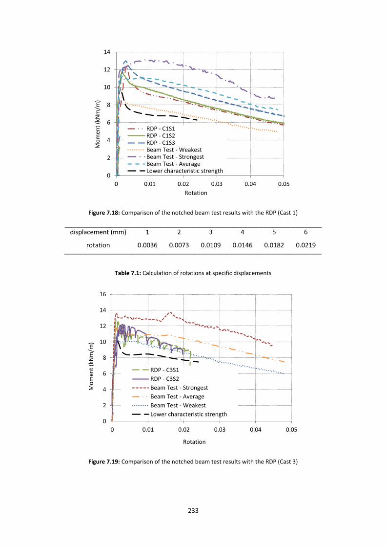
233
Figure 7.18: Comparison of the notched beam test results with the RDP (Cast 1)
displacement (mm) 1 2 3 4 5 6
rotation 0.0036 0.0073 0.0109 0.0146 0.0182 0.0219
Table 7.1: Calculation of rotations at specific displacements
Figure 7.19: Comparison of the notched beam test results with the RDP (Cast 3)
0
2
4
6
8
10
12
14
0 0.01 0.02 0.03 0.04 0.05
Mo
men
t (k
Nm
/m)
Rotation
RDP - C1S1 RDP - C1S2 RDP - C1S3 Beam Test - Weakest Beam Test - Strongest Beam Test - Average Lower characteristic strength
0
2
4
6
8
10
12
14
16
0 0.01 0.02 0.03 0.04 0.05
Mo
men
t (k
Nm
/m)
Rotation
RDP - C3S1
RDP - C3S2
Beam Test - Strongest
Beam Test - Average
Beam Test - Weakest
Lower characteristic strength
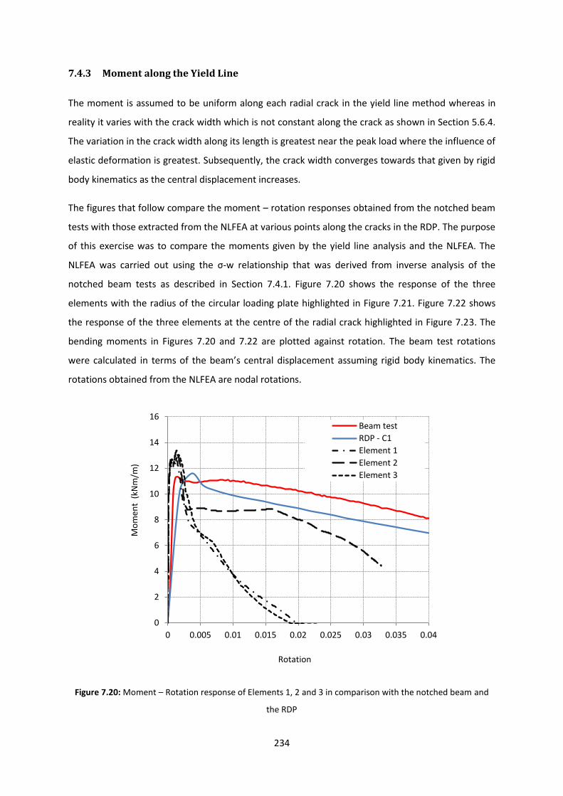
234
7.4.3 Moment along the Yield Line
The moment is assumed to be uniform along each radial crack in the yield line method whereas in
reality it varies with the crack width which is not constant along the crack as shown in Section 5.6.4.
The variation in the crack width along its length is greatest near the peak load where the influence of
elastic deformation is greatest. Subsequently, the crack width converges towards that given by rigid
body kinematics as the central displacement increases.
The figures that follow compare the moment – rotation responses obtained from the notched beam
tests with those extracted from the NLFEA at various points along the cracks in the RDP. The purpose
of this exercise was to compare the moments given by the yield line analysis and the NLFEA. The
NLFEA was carried out using the σ-w relationship that was derived from inverse analysis of the
notched beam tests as described in Section 7.4.1. Figure 7.20 shows the response of the three
elements with the radius of the circular loading plate highlighted in Figure 7.21. Figure 7.22 shows
the response of the three elements at the centre of the radial crack highlighted in Figure 7.23. The
bending moments in Figures 7.20 and 7.22 are plotted against rotation. The beam test rotations
were calculated in terms of the beam’s central displacement assuming rigid body kinematics. The
rotations obtained from the NLFEA are nodal rotations.
Figure 7.20: Moment – Rotation response of Elements 1, 2 and 3 in comparison with the notched beam and
the RDP
0
2
4
6
8
10
12
14
16
0 0.005 0.01 0.015 0.02 0.025 0.03 0.035 0.04
Mo
men
t (
kNm
/m)
Rotation
Beam test
RDP - C1
Element 1
Element 2
Element 3

235
Figure 7.21: Position of Elements 1, 2 and 3 within the Statically Determinate Round Plate
Figure 7.22: Moment – Rotation response of Elements 11, 12 and 13 in comparison with the notched beam
and the RDP
Figure 7.23: Position of Elements 11, 12 and 13 within the Statically Determinate Round Plate
Figures 7.20 and 7.22 show some differences between the moment – rotation responses of the
individual elements and the notched beam which are too great to be explained by the difference
between the predicted yield line and NLFEA responses shown in Figure 7.17. The following section
0
2
4
6
8
10
12
0 0.005 0.01 0.015 0.02 0.025 0.03 0.035 0.04
Mo
men
t (
kNm
/m)
Rotation
Beam Test
RDP - C1 Average
NLFEA - Element 11
NLFEA - Element 12
NLFEA - Element 13
3 2 1
11 13 12
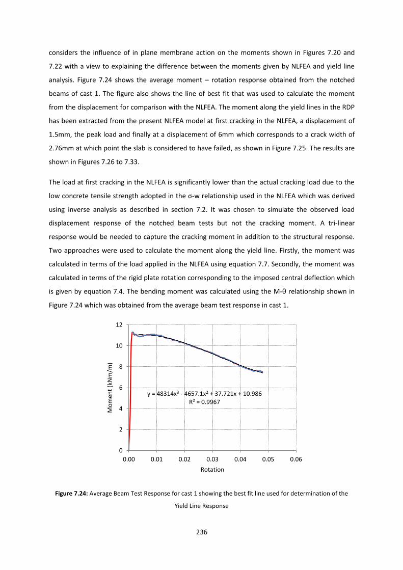
236
considers the influence of in plane membrane action on the moments shown in Figures 7.20 and
7.22 with a view to explaining the difference between the moments given by NLFEA and yield line
analysis. Figure 7.24 shows the average moment – rotation response obtained from the notched
beams of cast 1. The figure also shows the line of best fit that was used to calculate the moment
from the displacement for comparison with the NLFEA. The moment along the yield lines in the RDP
has been extracted from the present NLFEA model at first cracking in the NLFEA, a displacement of
1.5mm, the peak load and finally at a displacement of 6mm which corresponds to a crack width of
2.76mm at which point the slab is considered to have failed, as shown in Figure 7.25. The results are
shown in Figures 7.26 to 7.33.
The load at first cracking in the NLFEA is significantly lower than the actual cracking load due to the
low concrete tensile strength adopted in the σ-w relationship used in the NLFEA which was derived
using inverse analysis as described in section 7.2. It was chosen to simulate the observed load
displacement response of the notched beam tests but not the cracking moment. A tri-linear
response would be needed to capture the cracking moment in addition to the structural response.
Two approaches were used to calculate the moment along the yield line. Firstly, the moment was
calculated in terms of the load applied in the NLFEA using equation 7.7. Secondly, the moment was
calculated in terms of the rigid plate rotation corresponding to the imposed central deflection which
is given by equation 7.4. The bending moment was calculated using the M-θ relationship shown in
Figure 7.24 which was obtained from the average beam test response in cast 1.
Figure 7.24: Average Beam Test Response for cast 1 showing the best fit line used for determination of the
Yield Line Response
y = 48314x3 - 4657.1x2 + 37.721x + 10.986 R² = 0.9967
0
2
4
6
8
10
12
0.00 0.01 0.02 0.03 0.04 0.05 0.06
Mo
men
t (k
Nm
/m)
Rotation

237
The distribution of axial force normal to the direction of the crack (hoop force) at each load step has
also been plotted along the yield line to investigate the possible effect of membrane action on the
moment of resistance. To demonstrate the effect of the hoop force, the moments of resistance from
the notched beam test have been increased by the product of the hoop force (compression positive)
and half the slab depth.
Figures 7.26, 7.28, 7.30 and 7.32 compare the average moments along the yield line from the yield
line and NLFEA analyses. Figures 7.27, 7.29, 7.31 and 7.33 show the variation in hoop force along the
yield line at loads of 19.72kN, 70.3kN, 70.5kN and 68kN. The graphs show that the hoop forces were
relatively small but increased with increasing displacement. The resultant hoop forces along the
yield lines are close to zero as required for equilibrium. Figure 7.29 shows that at the peak load the
hoop force is compressive out to a radius of 400mm and tensile beyond that.
Figure 7.33 shows that the sign of the hoop force reverses at larger displacements becoming tensile
around the loading plate and compressive elsewhere which is consistent with the development of
tensile membrane action at larger displacements. The effect of the membrane forces on the
moment of resistance was investigated by adding 2Nh (where N denotes the axial force per unit
length and h denotes the depth of the section) to the moment calculated by inputting the rotation
from the NLFEA into the M-θ response of the notched beam. The results are shown in Figures 7.28,
7.30 and 7.32 which show that the resulting moments are almost equal to those extracted from the
NLFEA thus explaining the difference between the moments given by the NLFEA and yield line
analysis.
Figures 7.26, 7.28 and 7.30 also show that the average moment along the yield line in the NLFEA is
close to that calculated in terms of the rotation in the yield lines from equation 7.4 using the M-θ
relationship shown in Figure 7.24 from the beam tests.
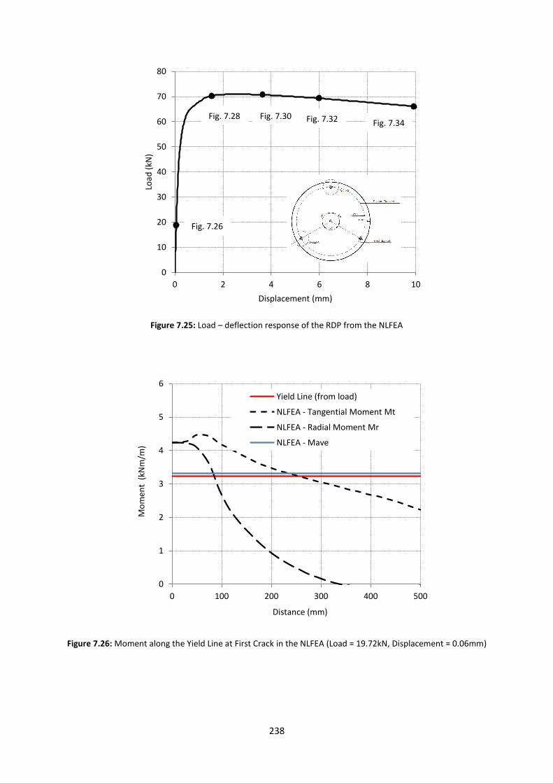
238
Figure 7.25: Load – deflection response of the RDP from the NLFEA
Figure 7.26: Moment along the Yield Line at First Crack in the NLFEA (Load = 19.72kN, Displacement = 0.06mm)
0
10
20
30
40
50
60
70
80
0 2 4 6 8 10
Load
(kN
)
Displacement (mm)
0
1
2
3
4
5
6
0 100 200 300 400 500
Mo
men
t (
kNm
/m)
Distance (mm)
Yield Line (from load)
NLFEA - Tangential Moment Mt
NLFEA - Radial Moment Mr
NLFEA - Mave
Fig. 7.26
Fig. 7.28 Fig. 7.32 Fig. 7.30 Fig. 7.34
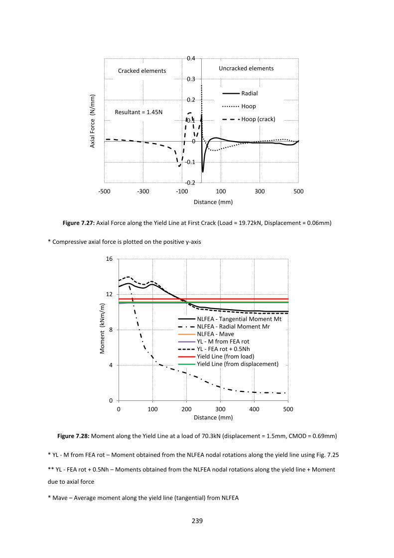
239
Figure 7.27: Axial Force along the Yield Line at First Crack (Load = 19.72kN, Displacement = 0.06mm)
* Compressive axial force is plotted on the positive y-axis
Figure 7.28: Moment along the Yield Line at a load of 70.3kN (displacement = 1.5mm, CMOD = 0.69mm)
* YL - M from FEA rot – Moment obtained from the NLFEA nodal rotations along the yield line using Fig. 7.25
** YL - FEA rot + 0.5Nh – Moments obtained from the NLFEA nodal rotations along the yield line + Moment
due to axial force
* Mave – Average moment along the yield line (tangential) from NLFEA
-0.2
-0.1
0
0.1
0.2
0.3
0.4
-500 -300 -100 100 300 500
Axi
al F
orc
e (
N/m
m)
Distance (mm)
Radial
Hoop
Hoop (crack)
0
4
8
12
16
0 100 200 300 400 500
Mo
men
t (
kNm
/m)
Distance (mm)
NLFEA - Tangential Moment Mt NLFEA - Radial Moment Mr NLFEA - Mave YL - M from FEA rot YL - FEA rot + 0.5Nh Yield Line (from load) Yield Line (from displacement)
Resultant = 1.45N
Uncracked elements Cracked elements

240
Figure 7.29: Axial Force along the Yield Line at a load of 70.3kN (displacement = 1.5mm, CMOD = 0.69mm)
Figure 7.30: Moment along the Yield Line at Peak Load (Load = 70.5kN, Displacement = 3.47mm, CMOD =
1.6mm)
-40
-20
0
20
40
60
80
-500 -300 -100 100 300 500
Axi
al F
orc
e (
N/m
m)
Distance (mm)
Radial
Hoop
Hoop (crack)
0
2
4
6
8
10
12
14
0 100 200 300 400 500
Mo
men
t (
kNm
/m)
Distance (mm)
NLFEA - Tangential Moment Mt
NLFEA - Radial Moment Mr
NLFEA - Mave
YL - M from FEA rot
YL - FEA rot + 0.5Nh
Yield Line (from load)
Yield Line (from displacement)
Resultant = 685N
Cracked elements Uncracked elements
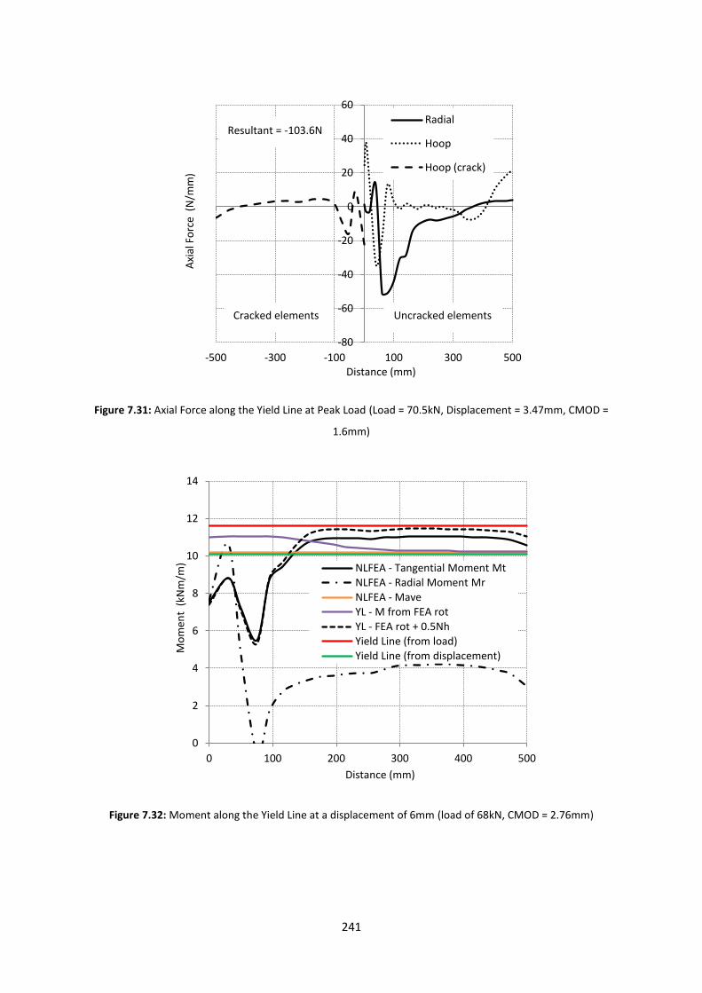
241
Figure 7.31: Axial Force along the Yield Line at Peak Load (Load = 70.5kN, Displacement = 3.47mm, CMOD =
1.6mm)
Figure 7.32: Moment along the Yield Line at a displacement of 6mm (load of 68kN, CMOD = 2.76mm)
-80
-60
-40
-20
0
20
40
60
-500 -300 -100 100 300 500
Axi
al F
orc
e (
N/m
m)
Distance (mm)
Radial
Hoop
Hoop (crack)
0
2
4
6
8
10
12
14
0 100 200 300 400 500
Mo
men
t (
kNm
/m)
Distance (mm)
NLFEA - Tangential Moment Mt NLFEA - Radial Moment Mr NLFEA - Mave YL - M from FEA rot YL - FEA rot + 0.5Nh Yield Line (from load) Yield Line (from displacement)
Resultant = -103.6N
Cracked elements Uncracked elements
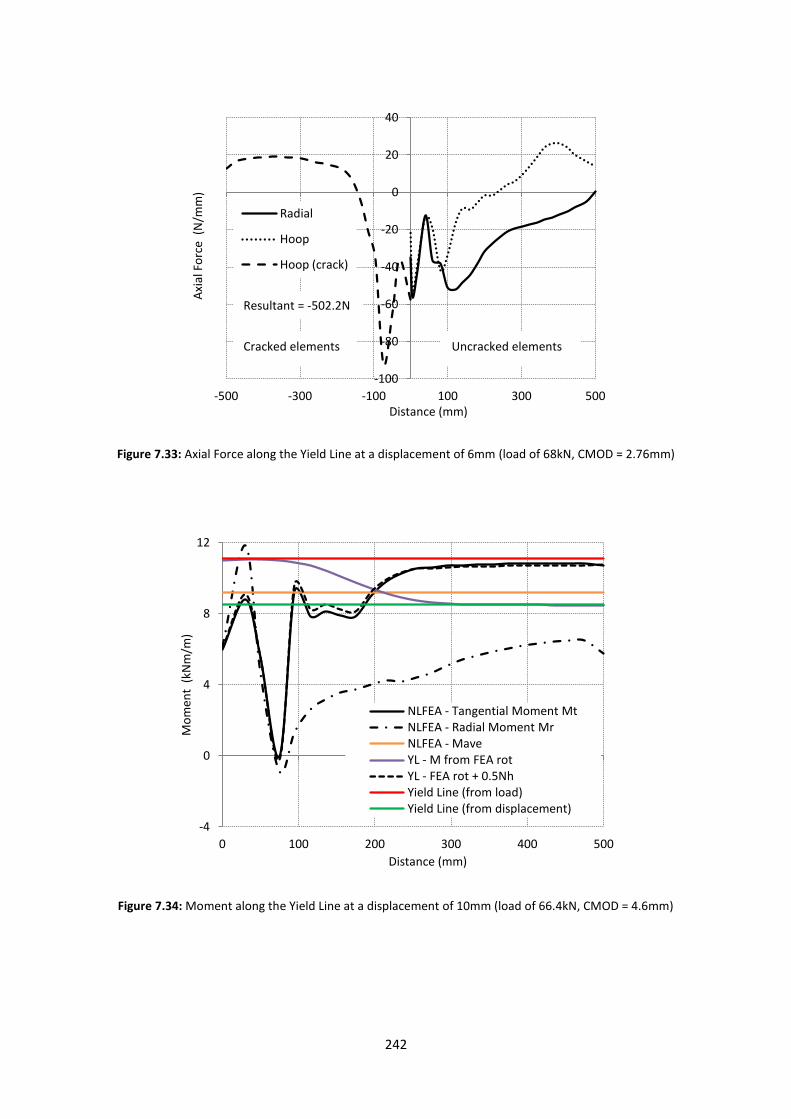
242
Figure 7.33: Axial Force along the Yield Line at a displacement of 6mm (load of 68kN, CMOD = 2.76mm)
Figure 7.34: Moment along the Yield Line at a displacement of 10mm (load of 66.4kN, CMOD = 4.6mm)
-100
-80
-60
-40
-20
0
20
40
-500 -300 -100 100 300 500
Axi
al F
orc
e (
N/m
m)
Distance (mm)
Radial
Hoop
Hoop (crack)
-4
0
4
8
12
0 100 200 300 400 500
Mo
men
t (
kNm
/m)
Distance (mm)
NLFEA - Tangential Moment Mt NLFEA - Radial Moment Mr NLFEA - Mave YL - M from FEA rot YL - FEA rot + 0.5Nh Yield Line (from load) Yield Line (from displacement)
Resultant = -502.2N
Cracked elements Uncracked elements

243
Figure 7.35: Axial force along the Yield Line at a displacement of 10mm (load of 66.4kN, CMOD = 4.6mm)
As stated at the beginning of the present section, the yield line method makes the assumption that
the moment is uniform along the cracks which form the yield lines. The NLFEA suggests that this is
not the case in reality but it seems a reasonable approximation as both methods give similar average
moments along the yield line when calculated at the same displacement. The axial force resultants
calculated show that the membrane forces are reasonably small, particularly at the earlier loading
stages but sufficient to account for the difference between the tangential moments given by the
NLFEA and yield line analysis. It is notable that the difference between the moments derived from
yield line analysis in terms of a) the imposed load and b) the imposed displacement increases with
increasing displacement. This difference is reflected in the divergence between the load resistances
given by NLFEA and yield line analysis in Figure 7.17. The increased load capacity given by the NLFEA
appears to be at least in part due to radial tensile membrane action evidence for which is provided
by the radial tensile forces in the uncracked elements shown in Figures 7.31, 7.33 and 7.35. There is
no doubt that the residual strength of the RDP can be increased by membrane action. It is however
unclear whether the membrane action observed in the NLFEA is realistic as it is clearly influenced by
the additional cracking which occurs in the NLFEA adjacent to the loading plate.
-200
-160
-120
-80
-40
0
40
80
-500 -300 -100 100 300 500
Axi
al F
orc
e (
N/m
m)
Distance (mm)
Radial
Hoop
Hoop (crack)
Resultant = -883N
Cracked elements Uncracked elements

244
7.4.4 Rotation along yield lines
A comparison was made between the rotations in the yield lines given by the NLFEA and the rigid
body kinematics of the yield line analysis. The yield line rotations were calculated in terms of the
actual plate deflection using equations 7.4 and 7.5. The NLFEA rotations were extracted from the
analysis. They are equal to twice the nodal rotation to either side of the crack. The results are given
in Figures 7.36 to 7.40.
The difference between the rotations is significant near the cracking load but reduces significantly
with increasing displacement. The crack widths are smaller below the peak load because the yield
line analysis assumes the slab to be fully cracked when it is not in reality. The yield line analysis also
overestimates rotations at small displacements as expected since it neglects elastic deformation
which is only significant at small displacements.
The ‘discontinuity’ that is observed at the centre of the RDP is due to the loading plate. All the
elements underneath the loading crack (Figure 7.15) causing the rotation to be distributed between
the elements rather than being concentrated in the three cracks.
Figure 7.36: Rotation along the Yield Line at First Crack (Load = 19.72kN, Displacement = 0.06mm)
0
0.00005
0.0001
0.00015
0.0002
0.00025
0.0003
0 100 200 300 400 500
Ro
tati
on
, UR
1
Distance (mm)
NLFEA
Yield Line Theory
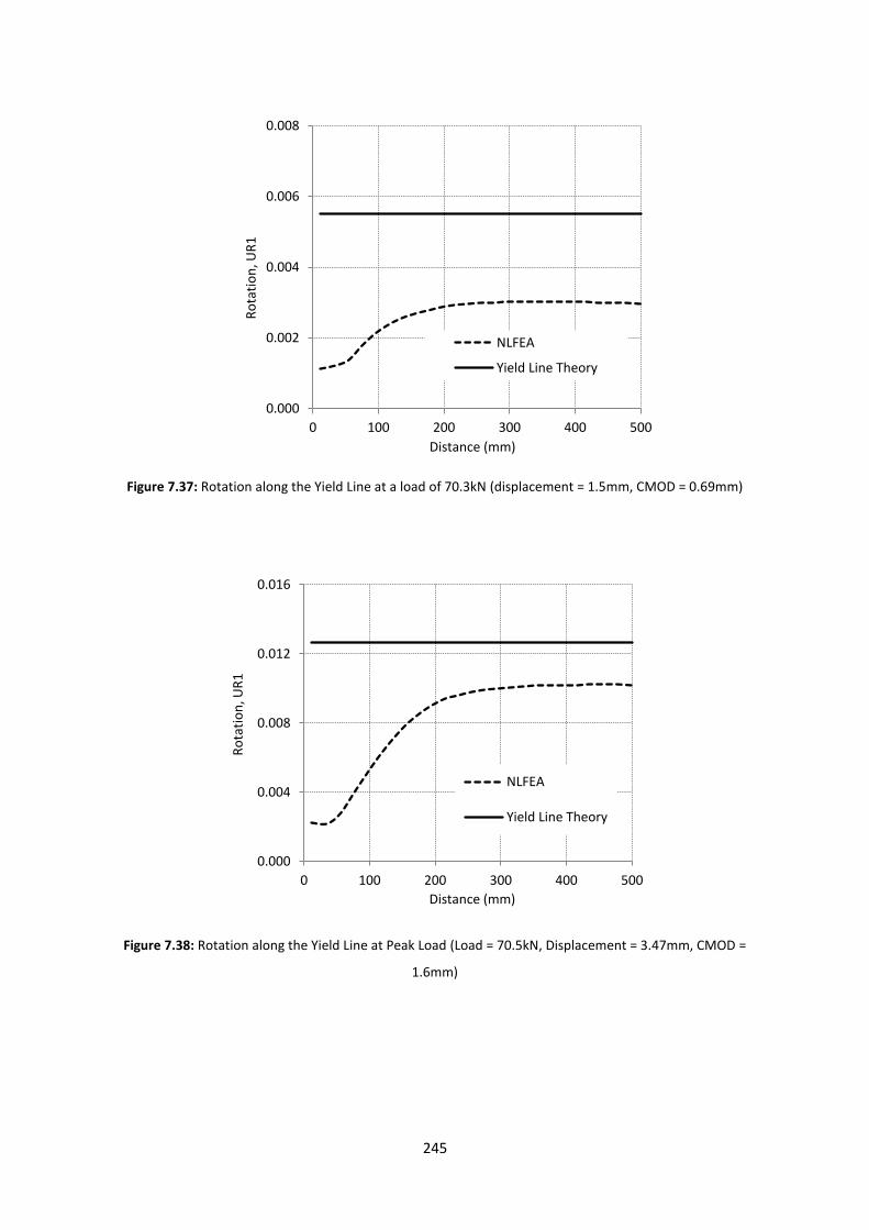
245
Figure 7.37: Rotation along the Yield Line at a load of 70.3kN (displacement = 1.5mm, CMOD = 0.69mm)
Figure 7.38: Rotation along the Yield Line at Peak Load (Load = 70.5kN, Displacement = 3.47mm, CMOD =
1.6mm)
0.000
0.002
0.004
0.006
0.008
0 100 200 300 400 500
Ro
tati
on
, UR
1
Distance (mm)
NLFEA
Yield Line Theory
0.000
0.004
0.008
0.012
0.016
0 100 200 300 400 500
Ro
tati
on
, UR
1
Distance (mm)
NLFEA
Yield Line Theory

246
Figure 7.39: Rotation along the Yield Line at a displacement of 6mm (load of 68kN, CMOD = 2.76mm)
Figure 7.40: Rotation along the Yield Line at a displacement of 10mm (load of 66.4kN, CMOD = 4.6mm)
0.000
0.005
0.010
0.015
0.020
0.025
0 100 200 300 400 500
Ro
tati
on
, UR
1
Distance (mm)
NLFEA
Yield Line Theory
0.000
0.010
0.020
0.030
0.040
0 100 200 300 400 500
Ro
tati
on
, UR
1
Distance (mm)
NLFEA
Yield Line Theory
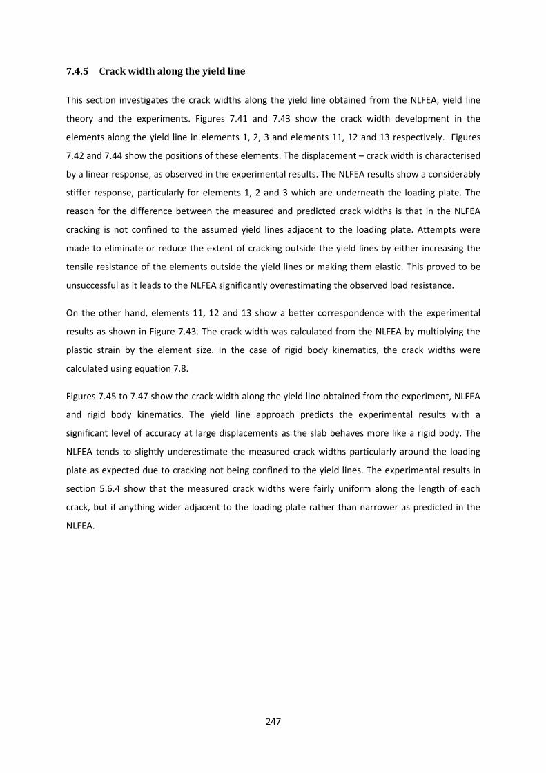
247
7.4.5 Crack width along the yield line
This section investigates the crack widths along the yield line obtained from the NLFEA, yield line
theory and the experiments. Figures 7.41 and 7.43 show the crack width development in the
elements along the yield line in elements 1, 2, 3 and elements 11, 12 and 13 respectively. Figures
7.42 and 7.44 show the positions of these elements. The displacement – crack width is characterised
by a linear response, as observed in the experimental results. The NLFEA results show a considerably
stiffer response, particularly for elements 1, 2 and 3 which are underneath the loading plate. The
reason for the difference between the measured and predicted crack widths is that in the NLFEA
cracking is not confined to the assumed yield lines adjacent to the loading plate. Attempts were
made to eliminate or reduce the extent of cracking outside the yield lines by either increasing the
tensile resistance of the elements outside the yield lines or making them elastic. This proved to be
unsuccessful as it leads to the NLFEA significantly overestimating the observed load resistance.
On the other hand, elements 11, 12 and 13 show a better correspondence with the experimental
results as shown in Figure 7.43. The crack width was calculated from the NLFEA by multiplying the
plastic strain by the element size. In the case of rigid body kinematics, the crack widths were
calculated using equation 7.8.
Figures 7.45 to 7.47 show the crack width along the yield line obtained from the experiment, NLFEA
and rigid body kinematics. The yield line approach predicts the experimental results with a
significant level of accuracy at large displacements as the slab behaves more like a rigid body. The
NLFEA tends to slightly underestimate the measured crack widths particularly around the loading
plate as expected due to cracking not being confined to the yield lines. The experimental results in
section 5.6.4 show that the measured crack widths were fairly uniform along the length of each
crack, but if anything wider adjacent to the loading plate rather than narrower as predicted in the
NLFEA.
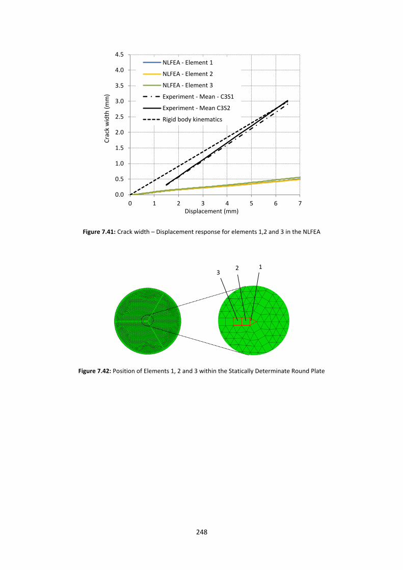
248
Figure 7.41: Crack width – Displacement response for elements 1,2 and 3 in the NLFEA
Figure 7.42: Position of Elements 1, 2 and 3 within the Statically Determinate Round Plate
0.0
0.5
1.0
1.5
2.0
2.5
3.0
3.5
4.0
4.5
0 1 2 3 4 5 6 7
Cra
ck w
idth
(m
m)
Displacement (mm)
NLFEA - Element 1
NLFEA - Element 2
NLFEA - Element 3
Experiment - Mean - C3S1
Experiment - Mean C3S2
Rigid body kinematics
3 2 1

249
Figure 7.43: Crack width – Displacement response for elements 11,12 and 13 in the NLFEA
Figure 7.44: Position of Elements 11, 12 and 13 within the Statically Determinate Round Plate
0.0
0.5
1.0
1.5
2.0
2.5
3.0
3.5
4.0
0 1 2 3 4 5 6 7
Cra
ck w
idth
(m
m)
Displacement (mm)
NLFEA - Element 11
NLFEA - Element 12
NLFEA - Element 13
Experiment - Mean - C3S1
Experiment - Mean C3S2
Rigid body kinematics
13 12 11
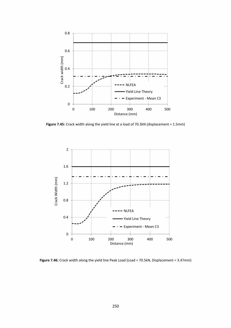
250
Figure 7.45: Crack width along the yield line at a load of 70.3kN (displacement = 1.5mm)
Figure 7.46: Crack width along the yield line Peak Load (Load = 70.5kN, Displacement = 3.47mm)
0
0.2
0.4
0.6
0.8
0 100 200 300 400 500
Cra
ck w
idth
(m
m)
Distance (mm)
NLFEA
Yield Line Theory
Experiment - Mean C3
0
0.4
0.8
1.2
1.6
2
0 100 200 300 400 500
Cra
ck W
idth
(m
m)
Distance (mm)
NLFEA
Yield Line Theory
Experiment - Mean C3

251
Figure 7.47: Crack width along the yield line at a displacement of 6mm (load of 68kN)
7.4.6 Derivation of EN 14651 residual concrete strengths from RDP tests
According to the recommendations of the Technical Report 34 (The Concrete Society, 2012), the
ultimate moment capacity can be calculated using the following expression:
14
2 16.029.0 rru bhM
(7.9)
where,
11 45.0 Rr f
(7.10)
44 37.0 Rr f
(7.11)
where, b denotes the width of the structural member and h denotes its depth. The residual
strengths 1Rf and
4Rf are determined from the notched beam test in accordance with the
recommendations of EN 14651 (British Standards Institution, 2005). 1Rf denotes the residual
strength at a CMOD of 0.5mm and 4Rf denotes the residual strength at a CMOD of 3.5mm.
0
0.5
1
1.5
2
2.5
3
0 100 200 300 400 500
Cra
ck w
idth
(m
m)
Distance (mm)
NLFEA
Yield Line Theory
Experiment - C3 Mean

252
On the other hand, MC2010 proposes that the ultimate moment of resistance should be taken as
that at a CMOD of 2.5mm but it gives the option of basing it on a lower user defined CMOD. Both
documents define a material safety factor of 1.5 for SFRC.
Residual concrete tensile strengths have been derived for each casting of RDP. This was done by
back calculating the moment of resistance along the yield lines at displacements corresponding to
CMOD of 0.5mm, 1.5mm, 2.5mm and 3.5mm. The procedure used to calculate the CMOD in the RDP
is analogous to that used in EN 14651 where the crack width is calculated in terms of the central
displacement as follows:
1. The displacement at which the RDP first cracked was assumed to equal that at which the load
displacement response first became non-linear.
2. The crack width was assumed to increase linearly with displacement from zero at first cracking
to the value of 0.46δ given by rigid body kinematics at a displacement of 7mm.
3. For displacements greater than 7mm, the crack width was calculated using rigid body kinematics
(equation 7.14).
First cracking is assumed to have occurred at displacements of 0.5mm in cast 1 and 0.8mm in cast 3.
Consequently, the CMOD was estimated as follows:
For displacements less than 7mm:
Cast 1 2477.04954.0 CMOD
(7.12)
Cast 3 4155.05194.0 CMOD
(7.13)
For displacements of more than 7mm:
46.0CMOD
(7.14)
Figures 7.48 and 7.49 show the crack width displacement response for slabs C3S1 and C3S2. The
mean crack width has been calculated and compared with the yield line analysis as well the assumed
responses given by equations 7.12 and 7.13 for casts 1 and 3 respectively. Figures 7.50 and 7.51
compare the CMOD’s given by equations 7.12 and 7.13 with those calculated assuming rigid body
kinematics.
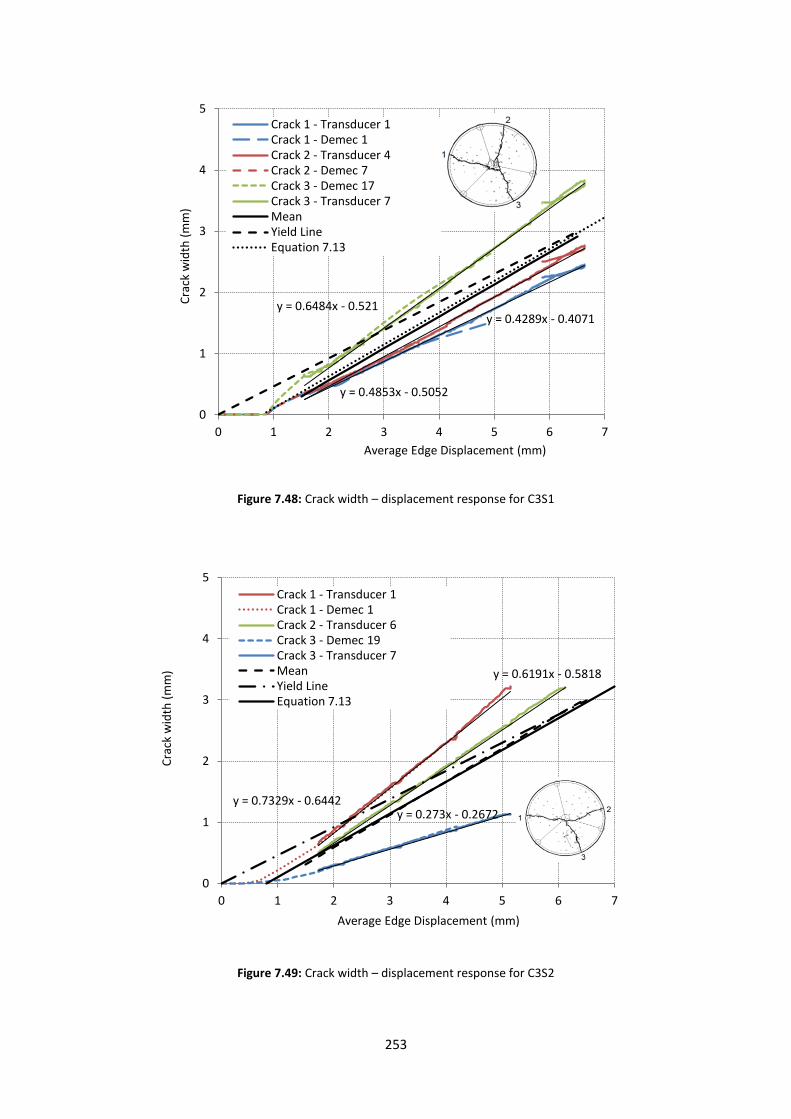
253
Figure 7.48: Crack width – displacement response for C3S1
Figure 7.49: Crack width – displacement response for C3S2
y = 0.4289x - 0.4071
y = 0.4853x - 0.5052
y = 0.6484x - 0.521
0
1
2
3
4
5
0 1 2 3 4 5 6 7
Cra
ck w
idth
(m
m)
Average Edge Displacement (mm)
Crack 1 - Transducer 1 Crack 1 - Demec 1 Crack 2 - Transducer 4 Crack 2 - Demec 7 Crack 3 - Demec 17 Crack 3 - Transducer 7 Mean Yield Line Equation 7.13
y = 0.7329x - 0.6442
y = 0.6191x - 0.5818
y = 0.273x - 0.2672
0
1
2
3
4
5
0 1 2 3 4 5 6 7
Cra
ck w
idth
(m
m)
Average Edge Displacement (mm)
Crack 1 - Transducer 1 Crack 1 - Demec 1 Crack 2 - Transducer 6 Crack 3 - Demec 19 Crack 3 - Transducer 7 Mean Yield Line Equation 7.13
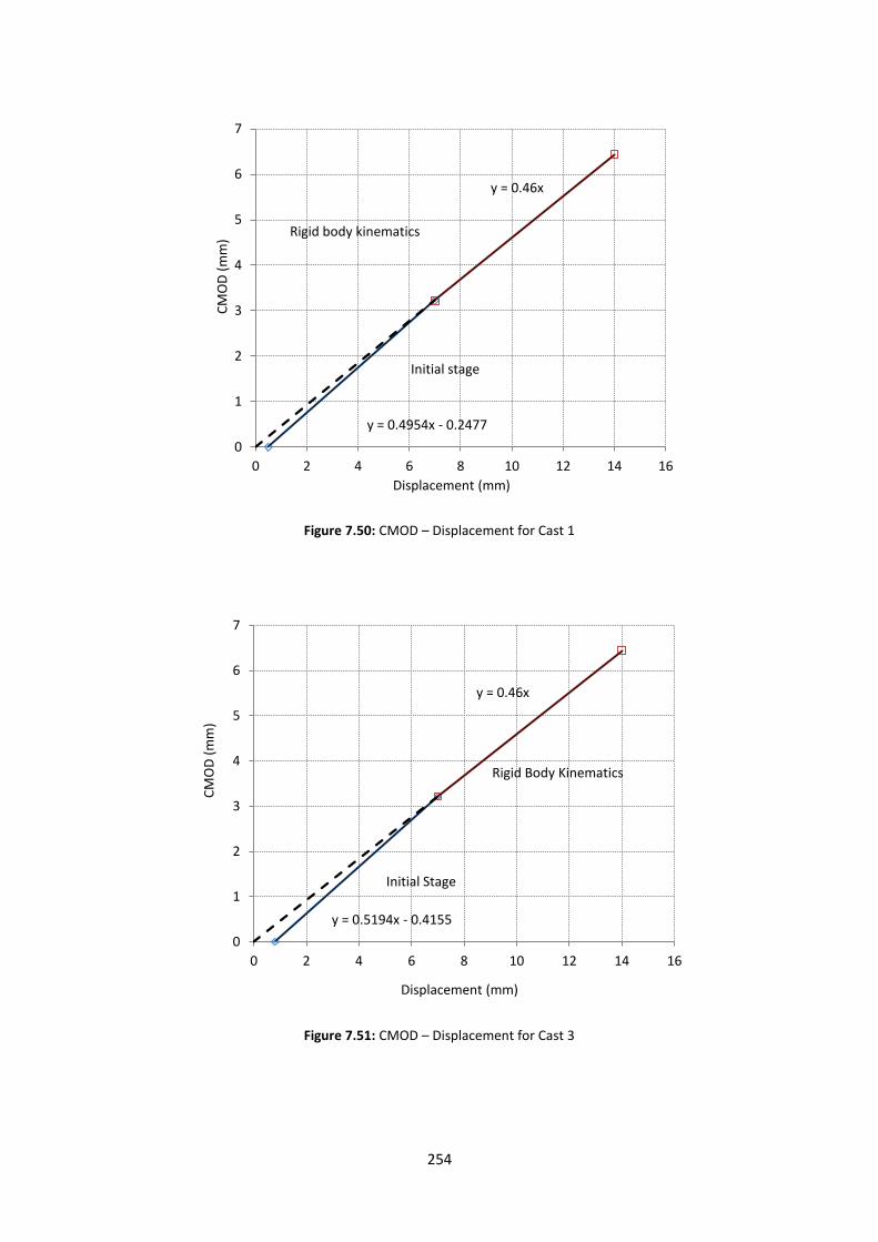
254
Figure 7.50: CMOD – Displacement for Cast 1
Figure 7.51: CMOD – Displacement for Cast 3
y = 0.4954x - 0.2477
y = 0.46x
0
1
2
3
4
5
6
7
0 2 4 6 8 10 12 14 16
CM
OD
(m
m)
Displacement (mm)
Initial stage
Rigid body kinematics
y = 0.5194x - 0.4155
y = 0.46x
0
1
2
3
4
5
6
7
0 2 4 6 8 10 12 14 16
CM
OD
(m
m)
Displacement (mm)
Initial Stage
Rigid Body Kinematics
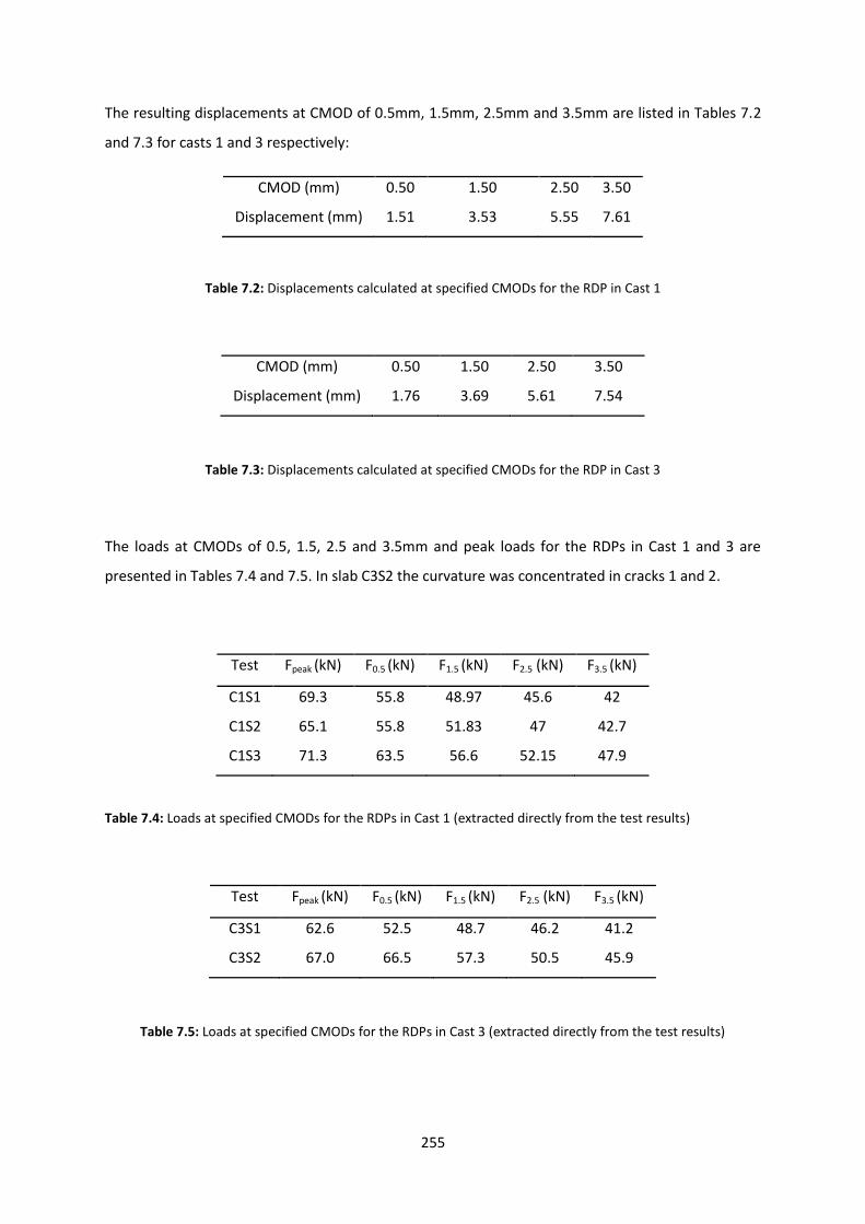
255
The resulting displacements at CMOD of 0.5mm, 1.5mm, 2.5mm and 3.5mm are listed in Tables 7.2
and 7.3 for casts 1 and 3 respectively:
CMOD (mm) 0.50 1.50 2.50 3.50
Displacement (mm) 1.51 3.53 5.55 7.61
Table 7.2: Displacements calculated at specified CMODs for the RDP in Cast 1
CMOD (mm) 0.50 1.50 2.50 3.50
Displacement (mm) 1.76 3.69 5.61 7.54
Table 7.3: Displacements calculated at specified CMODs for the RDP in Cast 3
The loads at CMODs of 0.5, 1.5, 2.5 and 3.5mm and peak loads for the RDPs in Cast 1 and 3 are
presented in Tables 7.4 and 7.5. In slab C3S2 the curvature was concentrated in cracks 1 and 2.
Test Fpeak (kN) F0.5 (kN) F1.5 (kN) F2.5 (kN) F3.5 (kN)
C1S1 69.3 55.8 48.97 45.6 42
C1S2 65.1 55.8 51.83 47 42.7
C1S3 71.3 63.5 56.6 52.15 47.9
Table 7.4: Loads at specified CMODs for the RDPs in Cast 1 (extracted directly from the test results)
Test Fpeak (kN) F0.5 (kN) F1.5 (kN) F2.5 (kN) F3.5 (kN)
C3S1 62.6 52.5 48.7 46.2 41.2
C3S2 67.0 66.5 57.3 50.5 45.9
Table 7.5: Loads at specified CMODs for the RDPs in Cast 3 (extracted directly from the test results)

256
The residual flexural stresses have been calculated by dividing the moment by the elastic section
modulus, Z. The resulting strengths are listed in Tables 7.6 and 7.7 for casts 1 and 3 respectively.
Test fL (MPa) f0.5 (MPa) f1.5 (MPa) f2.5 (MPa) f3.5 (MPa)
C1S1 4.6 3.7 3.3 3.0 2.8
C1S2 4.3 3.7 3.4 3.1 2.8
C1S3 4.7 4.2 3.8 3.5 3.2
Mean 4.6 3.9 3.5 3.2 2.9
Table 7.6: Residual strengths at specified CMODs in cast 1
Test fL (MPa) f0.5 (MPa) f1.5 (MPa) f2.5 (MPa) f3.5 (MPa)
C3S1 4.2 3.5 3.2 3.1 2.7
C3S2 4.5 4.4 3.8 3.4 3.1
Mean 4.3 4.0 3.5 3.2 2.9
Table 7.7: Residual strengths at specified CMODs in cast 3
7.4.7 Comparison of variability of residual strengths determined from RDP and notched
beams
Table 7.8 presents the mean, standard deviation and coefficient of variation of the maximum loads
and residual strengths for all the RDPs. The residual flexural strengths for the all the beam tests are
shown in Figures 5.3 to 5.7. The RDP tests exhibit a coefficient of variation of 4% (Table 7.8) whereas
the notched beams exhibit a variation of 12% (Table 5.7). This implies that a lower amount of
samples would need to be tested before a reasonable confidence level is achieved. The variation in
crack patterns in the RDP, examined in Chapter Five, does not affect significantly the overall load –
deflection response.
Figures 7.52 and 7.53 compare the residual strengths obtained from the RDP and beam tests for
casts 1 and 3. The residual strength for the notched beam tests have been calculated using the EN
14651 method, described in Section 2.4.2. The residual strengths obtained from the beam tests

257
(Tables 5.3 to 5.6) are significantly greater than the RDP, particularly for crack widths beyond 1mm.
For larger crack widths, the residual strengths exhibit a greater divergence. This is consistent with
the overestimate in strength that was found when predicting the response of the RDP using material
properties derived in the notched beam tests. This is due to the beam not being allowed to fail at its
weakest section due to the sawing of the notch unlike the RDP where the position of cracks is not
predetermined. This suggests that the notched beam tests may give an unsafe estimate of the
concrete residual strength.
Figure 7.54 shows the variation in residual strengths obtained from casts 1 and 3. The residual
strengths corresponding to casts 1 and 3 are almost identical which serves as a good indicator of the
consistency of the concrete mixing procedures used. Figure 7.55 compares the residual strengths of
all the RDP and notched beam tests. With the exception of cast 2, all the other castings exhibit
considerably higher residual strengths than the RDPs. In addition, the mean residual strength for
cast 1 and 3 for the notched beam tests are shown to be nearly identical.
In the yield line analysis a moment – rotation response was back calculated from the load deflection
responses of the RDP and the notched beam tests assuming rigid body kinematics. Conversely in the
derivation of residual strengths, the resistance is calculated at actual crack widths which are less
than those calculated from rigid body kinematics. The elastic deformation was neglected in the
calculation of crack width since it was relatively small compared with the overall deformation. In
design, the strength is calculated at a specified CMOD of 2.5 mm in MC2010 (though other CMOD
are allowed at the discretion of the designer) or in terms of an average flexural strength in TR34.
Maximum Load
(kN)
Flexural strength
(N/mm2)
fR1
(N/mm2)
fR2
(N/mm2)
fR3
(N/mm2)
fR4
(N/mm2)
Mean 66.67 4.46 3.91 3.50 3.21 2.92
St. Dev 2.66 0.18 0.28 0.17 0.14 0.14
Coef. Var. 0.04 0.04 0.07 0.05 0.04 0.05
Table 7.8: Mean, standard deviation and coefficient of variation for all RDP tests
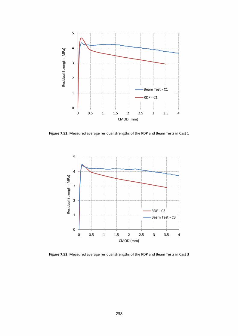
258
Figure 7.52: Measured average residual strengths of the RDP and Beam Tests in Cast 1
Figure 7.53: Measured average residual strengths of the RDP and Beam Tests in Cast 3
0
1
2
3
4
5
0 0.5 1 1.5 2 2.5 3 3.5 4
Res
idu
al S
tren
gth
(M
Pa)
CMOD (mm)
Beam Test - C1
RDP - C1
0
1
2
3
4
5
0 0.5 1 1.5 2 2.5 3 3.5 4
Res
idu
al S
tren
gth
(M
Pa)
CMOD (mm)
RDP - C3
Beam Test - C3

259
Figure 7.54: Comparison of the measured CMOD – Mean residual strengths for Casts 1 and 3 (RDP)
Figure 7.55: Mean residual strengths of the notched beams and RDP in all castings
Subsequently, the peak moment obtained in the RDP experiment has been compared to the
ultimate and design moments proposed by Technical Report 34 (The Concrete Society, 2012) and
Model Code 2010 (International Federation for Structural Concrete, 2010) (Tables 7.9 and 7.10). The
design moments of resistance obtained from Technical Report 34 and Model Code 2010 are
calculated for cracked sections and are therefore less than the peak moments obtained in the tests.
0
1
2
3
4
5
0 0.5 1 1.5 2 2.5 3 3.5 4
Res
idu
al S
tren
gth
(M
Pa)
CMOD (mm)
RDP - C3
RDP - C1
0
1
2
3
4
5
0 1 2 3 4 5 6 7 8
Res
idu
al S
tren
gth
(M
Pa)
CMOD (mm)
RDP - C3
RDP - C1
Beam Test - C1
Beam Test - C2
Beam Test - C3
Beam Test - C4
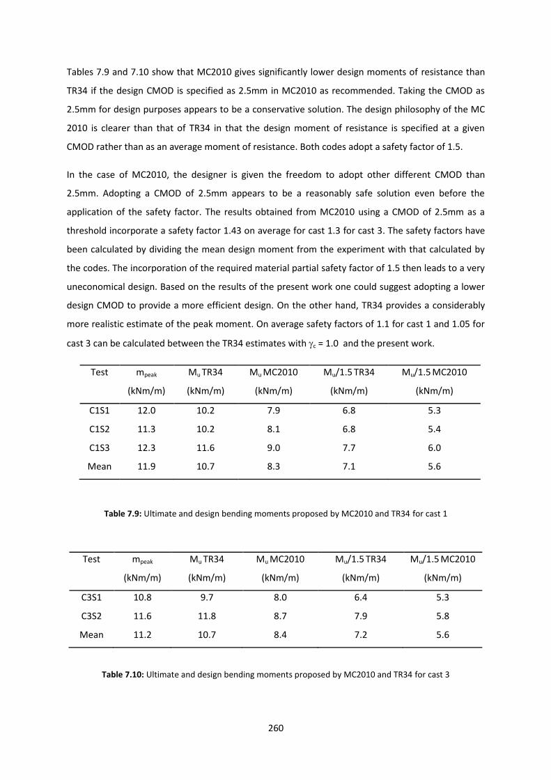
260
Tables 7.9 and 7.10 show that MC2010 gives significantly lower design moments of resistance than
TR34 if the design CMOD is specified as 2.5mm in MC2010 as recommended. Taking the CMOD as
2.5mm for design purposes appears to be a conservative solution. The design philosophy of the MC
2010 is clearer than that of TR34 in that the design moment of resistance is specified at a given
CMOD rather than as an average moment of resistance. Both codes adopt a safety factor of 1.5.
In the case of MC2010, the designer is given the freedom to adopt other different CMOD than
2.5mm. Adopting a CMOD of 2.5mm appears to be a reasonably safe solution even before the
application of the safety factor. The results obtained from MC2010 using a CMOD of 2.5mm as a
threshold incorporate a safety factor 1.43 on average for cast 1.3 for cast 3. The safety factors have
been calculated by dividing the mean design moment from the experiment with that calculated by
the codes. The incorporation of the required material partial safety factor of 1.5 then leads to a very
uneconomical design. Based on the results of the present work one could suggest adopting a lower
design CMOD to provide a more efficient design. On the other hand, TR34 provides a considerably
more realistic estimate of the peak moment. On average safety factors of 1.1 for cast 1 and 1.05 for
cast 3 can be calculated between the TR34 estimates with c = 1.0 and the present work.
Test mpeak
(kNm/m)
Mu TR34
(kNm/m)
Mu MC2010
(kNm/m)
Mu/1.5 TR34
(kNm/m)
Mu/1.5 MC2010
(kNm/m)
C1S1 12.0 10.2 7.9 6.8 5.3
C1S2 11.3 10.2 8.1 6.8 5.4
C1S3
Mean
12.3
11.9
11.6
10.7
9.0
8.3
7.7
7.1
6.0
5.6
Table 7.9: Ultimate and design bending moments proposed by MC2010 and TR34 for cast 1
Test mpeak
(kNm/m)
Mu TR34
(kNm/m)
Mu MC2010
(kNm/m)
Mu/1.5 TR34
(kNm/m)
Mu/1.5 MC2010
(kNm/m)
C3S1 10.8 9.7 8.0 6.4 5.3
C3S2 11.6 11.8 8.7 7.9 5.8
Mean 11.2 10.7 8.4 7.2 5.6
Table 7.10: Ultimate and design bending moments proposed by MC2010 and TR34 for cast 3

261
7.5 Smeared Cracking Inverse Analysis of the RDP
7.5.1 General Overview
This section describes the inverse analysis modelling procedure used for the statically determinate
round panel test. The experimental setup for this test is illustrated in Figure 7.56. The inverse
analysis was carried out using the procedure described in Section 7.2 and illustrated in Figure 7.2. A
preliminary study was undertaken which suggested that it was possible to capture the load –
displacement response of the RDP with a bi-linear σ-w relationship. Therefore, the tri-linear
response shown in Figure 7.57 was adopted.
Figure 7.56: Test arrangement adopted for the statically determinate round panel test
Figure 7.57: Tension softening response assumed for the statically determinate round panel inverse analysis
procedure
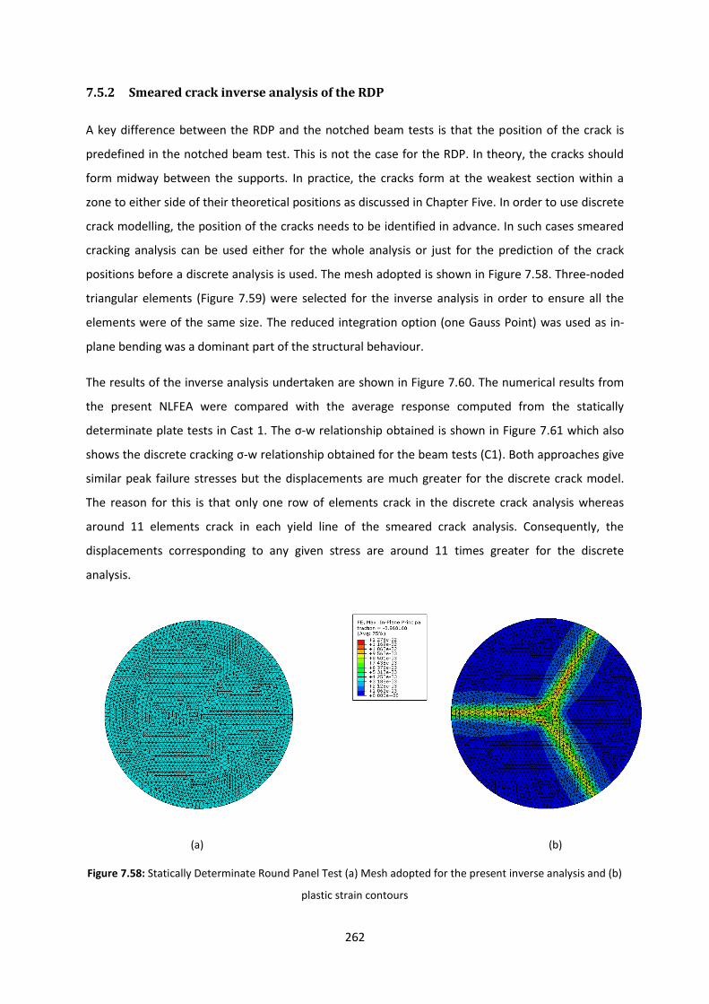
262
7.5.2 Smeared crack inverse analysis of the RDP
A key difference between the RDP and the notched beam tests is that the position of the crack is
predefined in the notched beam test. This is not the case for the RDP. In theory, the cracks should
form midway between the supports. In practice, the cracks form at the weakest section within a
zone to either side of their theoretical positions as discussed in Chapter Five. In order to use discrete
crack modelling, the position of the cracks needs to be identified in advance. In such cases smeared
cracking analysis can be used either for the whole analysis or just for the prediction of the crack
positions before a discrete analysis is used. The mesh adopted is shown in Figure 7.58. Three-noded
triangular elements (Figure 7.59) were selected for the inverse analysis in order to ensure all the
elements were of the same size. The reduced integration option (one Gauss Point) was used as in-
plane bending was a dominant part of the structural behaviour.
The results of the inverse analysis undertaken are shown in Figure 7.60. The numerical results from
the present NLFEA were compared with the average response computed from the statically
determinate plate tests in Cast 1. The σ-w relationship obtained is shown in Figure 7.61 which also
shows the discrete cracking σ-w relationship obtained for the beam tests (C1). Both approaches give
similar peak failure stresses but the displacements are much greater for the discrete crack model.
The reason for this is that only one row of elements crack in the discrete crack analysis whereas
around 11 elements crack in each yield line of the smeared crack analysis. Consequently, the
displacements corresponding to any given stress are around 11 times greater for the discrete
analysis.
(a) (b)
Figure 7.58: Statically Determinate Round Panel Test (a) Mesh adopted for the present inverse analysis and (b)
plastic strain contours

263
Figure 7.59: Element adopted for present inverse analysis
Figure 7.60: Results of inverse analysis of the statically determinate round panel test
Figure 7.61: Stress – displacement response obtained from the inverse analysis
0
20
40
60
80
0 10 20 30 40
Load
(kN
)
Displacement (mm)
Present NLFEA - Inverse analysis
C1 - Average
0
0.4
0.8
1.2
1.6
0 5 10 15
Stre
ss (
N/m
m2 )
Displacement (mm)
Smeared cracking
Discrete cracking
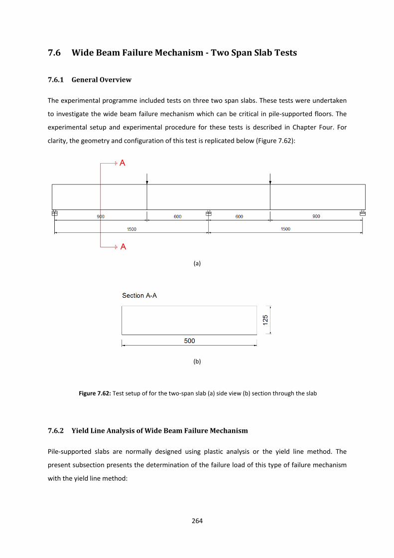
264
7.6 Wide Beam Failure Mechanism - Two Span Slab Tests
7.6.1 General Overview
The experimental programme included tests on three two span slabs. These tests were undertaken
to investigate the wide beam failure mechanism which can be critical in pile-supported floors. The
experimental setup and experimental procedure for these tests is described in Chapter Four. For
clarity, the geometry and configuration of this test is replicated below (Figure 7.62):
(a)
(b)
Figure 7.62: Test setup of for the two-span slab (a) side view (b) section through the slab
7.6.2 Yield Line Analysis of Wide Beam Failure Mechanism
Pile-supported slabs are normally designed using plastic analysis or the yield line method. The
present subsection presents the determination of the failure load of this type of failure mechanism
with the yield line method:
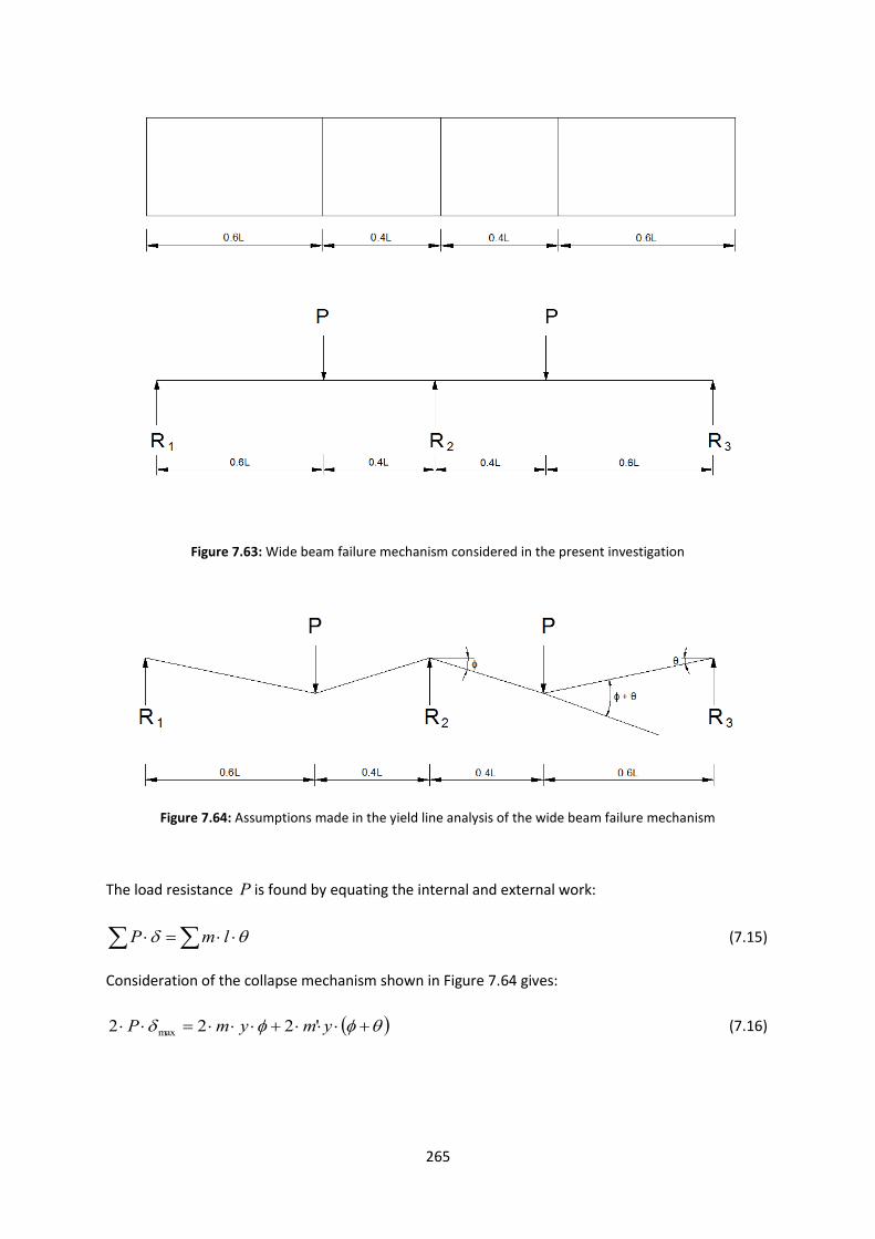
265
Figure 7.63: Wide beam failure mechanism considered in the present investigation
Figure 7.64: Assumptions made in the yield line analysis of the wide beam failure mechanism
The load resistance P is found by equating the internal and external work:
lmP
(7.15)
Consideration of the collapse mechanism shown in Figure 7.64 gives:
ymymP '222 max
(7.16)
266
Where, P denotes the load, y denotes the width of the beam, max denotes the vertical deflection,
m and 'm denote the sagging and hogging moments respectively and and denote the angles of
rotation of each of the rigid bodies, as illustrated in Figure 7.64.
From simple trigonometry, the angles and can be expressed in terms of the vertical deflection
max , thus:
L6.0
max
(7.17)
L4.0
max
(7.18)
Substituting equations (7.15) and (7.16) into equation (7.14) and cancelling out the common terms
gives the following expression:
yLL
mL
mP
6.0
1
4.0
1'
4.0
(7.19)
ymmL
P
'
3
5
2
5
(7.20)
7.6.4 Smeared Cracking Approach
The first numerical modelling approach considered herein is the smeared cracking method. The
benefit of using a smeared crack approach over a discrete crack one is that no prior knowledge is
required of the critical flexural failure mechanism. The disadvantage is that the analysis does not
capture the discrete nature of cracking in SFRC slabs without conventional reinforcement. Therefore,
crack widths cannot be directly extracted from the analysis.
The stress-displacement response obtained from the smeared crack inverse analysis of the statically
determinate round panel test (Figure 7.61) has been incorporated into the NLFEA model for the two-
span slab. The element type of choice was the S3R (Three-noded triangular element with reduced
integration) as illustrated in Figure 7.59. The elements with reduced integration have a single Gauss
point at the centre of the element. This option was activated to prevent possible shear locking
effects, as bending is dominant. The element size was 20mm using the mesh shown in Figure 7.65.
The mesh size was the same as used in the smeared cracking analysis of the RDP.

267
Figure 7.65: Mesh adopted for the smeared cracking model of the two-span slab
(a) (b)
Figure 7.66: Crack pattern (a) at the underside and (b) on the topside of the two span slab
Figure 7.66 shows that the crack patterns predicted by the NLFEA are consistent with those
observed in the tests. Two slabs were tested without axial restraint as described in Chapter Four.
Figure 7.67 shows that their load-deflection responses were quite different. Inspection of the
fracture cross-section after the experiment indicated that the majority of the steel fibres in test C4S1
had ‘sunk’ to the bottom of the slab causing the section to have a significantly lower residual
moment capacity after cracking than expected. Furthermore, in slab C4S1 only one span cracked
during the experiment.
Figure 7.67 shows good agreement between the results of the yield line and the NLFEA responses.
The non-linear response shown in Figure 7.67 was calculated with beam theory assuming the beam
behaves elastically between hinges. A benefit of using NLFEA over yield line analysis is that it gives
the sequence of crack formation unlike yield line analysis which only considers the response of a
fully cracked slab.
A yield line analysis was carried out to determine whether the observed variation in the strengths of
the two span beams is consistent with the variation in material properties observed in the notched

268
beam tests. The results of the analyses are given in Figure 7.68 which shows that the strengths of the
continuous slabs lie between the strengths calculated from the moment – rotation relationships
from the strongest and weakest beam tests.
Figure 7.67: Load – Displacement Response
Figure 7.68: Comparison of beam and two span slab tests in cast 4
0
10
20
30
40
50
60
70
0 2.5 5 7.5 10 12.5 15 17.5 20
Load
(kN
)
Displacement (mm)
C4S1 C4S3 Present NLFEA Yield Line Non-linear beam analysis
0
10
20
30
40
50
60
0 2.5 5 7.5 10 12.5 15 17.5 20
Load
(kN
)
Displacement (mm)
Experiment - C4S1
Experiment - C4S3
YL - Beam Test - Weakest C4
YL - Beam test - Strongest C4

269
7.6.5 Discrete Cracking Approach
The second approach considered herein is the discrete cracking approach which has the major
drawback that it requires prior knowledge of the crack pattern. However, this can prove to be an
advantage, once the crack pattern is known as the mesh can be locally refined where required saving
computational time.
Figure 7.69: Mesh adopted for the discrete cracking model of the two-span slab
(a) (b)
Figure 7.70: Crack pattern (a) at the underside and (b) on the topside of the two span slab
The discretization was straightforward in this case as the cracks were known to occur at the point of
loading as well as the central support. The slab was forced to crack in these places by increasing the
tensile strength of the concrete elsewhere. The aim of this exercise was to ensure that only one

270
column of elements cracked making the model analogous with the discrete cracking procedure used
for the three point bending notched beam test. Four-noded rectangular elements of size 20mm x
20mm with reduced integration (S4R) (Figure 7.4 (a)) were used. Elsewhere three-noded triangular
elements were used with reduced integration (S3R) (Figure 7.4(b)).
Figure 7.71 illustrates the load-deflection response from the present NLFEA model. It compares the
experimental response with those given by NLFEA and yield line analysis. For the computation of the
load – deflection response using the yield line method, the ‘average’ moment rotation response of
the corresponding beam tests was used (Cast C4). This was substituted in equations 7.11, 7.12 and
7.14 in order to obtain the structural response. Figure 7.71 shows that the results of the discrete
crack NLFEA compare favourably with the results of the smeared crack analysis. The results also
compare favourably with the yield line analysis for displacements greater than 1mm. The σ-w
response obtained from the smeared crack analysis gave good results for the two span slab because
the element size was the same and a similar number of elements cracked perpendicular to the crack
width.
Figure 7.74 compares the responses of the two span slab with the highest and lowest beam
responses in Cast Four. The responses of both slabs fall within the notched beam ‘envelope'. It is
noticeable that the measured response of slab C4S1 is nearly identical to that calculated using the
material properties derived from the weakest notched beam test.
A comparison has been made between the measured and predicted moment – rotation responses at
the central support and mid-span. The experimental moments were calculated in terms of the
reactions under each support which were measured using load cells. Figure 7.74 shows that slab
C4S1 exhibited a significant softer behaviour than the NLFEA model.
On the other hand, two cracks were observed in the case of C4S3. The moment – rotation response
of this appears to be more consistent with the present NLFEA. This was also reflected in the load –
deflection response of the slab. The peak load achieved with this slab is close to the present NLFEA
predictions, however this load is not sustained. The root of this issue was the poor dispersion of the
steel fibres which reduced the residual moment of resistance after cracking.
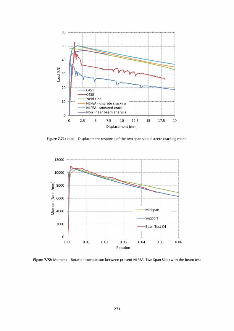
271
Figure 7.71: Load – Displacement response of the two span slab discrete cracking model
Figure 7.72: Moment – Rotation comparison between present NLFEA (Two Span Slab) with the beam test
0
10
20
30
40
50
60
0 2.5 5 7.5 10 12.5 15 17.5 20
Load
(kN
)
Displacement (mm)
C4S1 C4S3 Yield Line NLFEA - discrete cracking NLFEA - smeared crack Non linear beam analysis
0
2000
4000
6000
8000
10000
12000
0.00 0.01 0.02 0.03 0.04 0.05 0.06
Mo
men
t (N
mm
/mm
)
Rotation
Midspan
Support
BeamTest C4
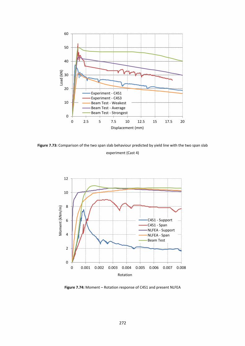
272
Figure 7.73: Comparison of the two span slab behaviour predicted by yield line with the two span slab
experiment (Cast 4)
Figure 7.74: Moment – Rotation response of C4S1 and present NLFEA
0
10
20
30
40
50
60
0 2.5 5 7.5 10 12.5 15 17.5 20
Load
(kN
)
Displacement (mm)
Experiment - C4S1 Experiment - C4S3 Beam Test - Weakest Beam Test - Average Beam Test - Strongest
0
2
4
6
8
10
12
0 0.001 0.002 0.003 0.004 0.005 0.006 0.007 0.008
Mo
men
t (k
Nm
/m)
Rotation
C4S1 - Support C4S1 - Span NLFEA - Support NLFEA - Span Beam Test
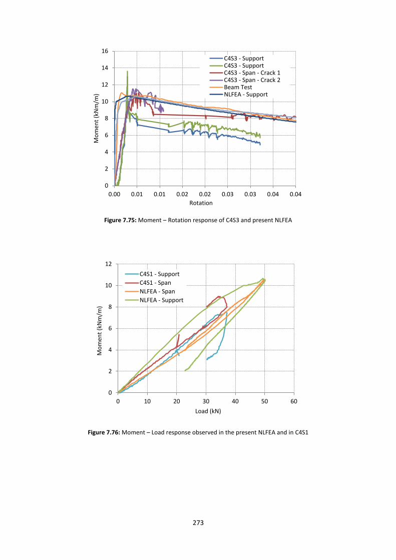
273
Figure 7.75: Moment – Rotation response of C4S3 and present NLFEA
Figure 7.76: Moment – Load response observed in the present NLFEA and in C4S1
0
2
4
6
8
10
12
14
16
0.00 0.01 0.01 0.02 0.02 0.03 0.03 0.04 0.04
Mo
men
t (k
Nm
/m)
Rotation
C4S3 - Support C4S3 - Support C4S3 - Span - Crack 1 C4S3 - Span - Crack 2 Beam Test NLFEA - Support
0
2
4
6
8
10
12
0 10 20 30 40 50 60
Mo
men
t (k
Nm
/m)
Load (kN)
C4S1 - Support
C4S1 - Span
NLFEA - Span
NLFEA - Support

274
Figure 7.77: Moment – Load response observed in the present NLFEA and in C4S3
7.6.6 Comparison of predicted and measured crack widths
This section presents a comparison between the measured and predicted crack widths from the
NLFEA and yield line theory. The crack width displacement responses of slabs C4S1 and C4S3 are
shown in Figures 7.78 to 7.81. The displacement – crack width is characterised by a linear response.
The predicted crack widths from rigid body kinematics and NLFEA are comparable. This suggests that
the yield line method is a good alternative to the NLFEA with the added advantage that it is relatively
straightforward to implement. In the case of Figure 7.78, the crack widths were given by NLFEA and
yield line analysis agree poorly with the experimental results since only one span cracked as
discussed previously. The effect of this is to approximately halve the crack width at the support since
the support rotation is halved. The comparison between the measured and predicted crack widths is
much better for slab C4S3 in Figure 7.79 since both spans cracked. The experimental deflection at
first cracking is excessive due to bedding in effects which have not been corrected.
0
2
4
6
8
10
12
14
0 10 20 30 40 50 60
Mo
men
t (k
Nm
/m)
Load (kN)
C4S3 - Span - Crack 1
C4S3 - Span - Crack 2
NLFEA - Span
NLFEA - Support

275
Figure 7.78: Crack width displacement response at the support for slab C4S1
Figure 7.79: Crack width displacement response at the support for slab C4S3
0.0
0.5
1.0
1.5
2.0
2.5
3.0
0 2 4 6 8
Cra
ck w
idth
(m
m)
Displacement (mm)
Experiment C4S1
NLFEA
Yield Line Theory
0.0
0.5
1.0
1.5
2.0
2.5
3.0
0 2 4 6 8
Cra
ck w
idth
(m
m)
Displacement (mm)
Experiment C4S3
NLFEA
Yield Line Theory
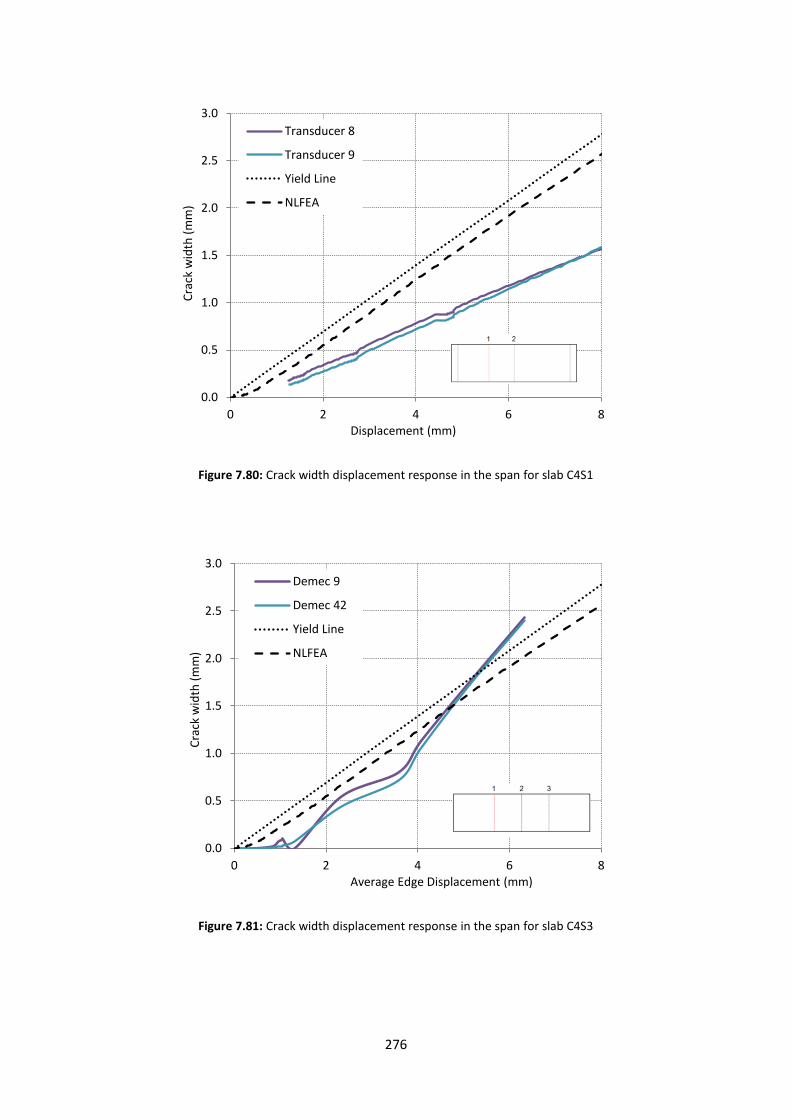
276
Figure 7.80: Crack width displacement response in the span for slab C4S1
Figure 7.81: Crack width displacement response in the span for slab C4S3
0.0
0.5
1.0
1.5
2.0
2.5
3.0
0 2 4 6 8
Cra
ck w
idth
(m
m)
Displacement (mm)
Transducer 8
Transducer 9
Yield Line
NLFEA
0.0
0.5
1.0
1.5
2.0
2.5
3.0
0 2 4 6 8
Cra
ck w
idth
(m
m)
Average Edge Displacement (mm)
Demec 9
Demec 42
Yield Line
NLFEA
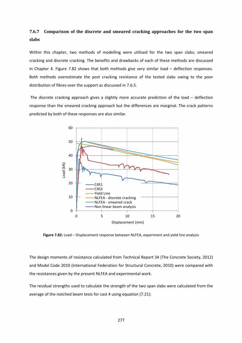
277
7.6.7 Comparison of the discrete and smeared cracking approaches for the two span
slabs
Within this chapter, two methods of modelling were utilised for the two span slabs; smeared
cracking and discrete cracking. The benefits and drawbacks of each of these methods are discussed
in Chapter 4. Figure 7.82 shows that both methods give very similar load – deflection responses.
Both methods overestimate the post cracking resistance of the tested slabs owing to the poor
distribution of fibres over the support as discussed in 7.6.5.
The discrete cracking approach gives a slightly more accurate prediction of the load – deflection
response than the smeared cracking approach but the differences are marginal. The crack patterns
predicted by both of these responses are also similar.
Figure 7.82: Load – Displacement response between NLFEA, experiment and yield line analysis
The design moments of resistance calculated from Technical Report 34 (The Concrete Society, 2012)
and Model Code 2010 (International Federation for Structural Concrete, 2010) were compared with
the resistances given by the present NLFEA and experimental work.
The residual strengths used to calculate the strength of the two span slabs were calculated from the
average of the notched beam tests for cast 4 using equation (7.21):
0
10
20
30
40
50
60
0 5 10 15 20
Load
(kN
)
Displacement (mm)
C4S1 C4S3 Yield Line NLFEA - discrete cracking NLFEA - smeared crack Non linear beam analysis
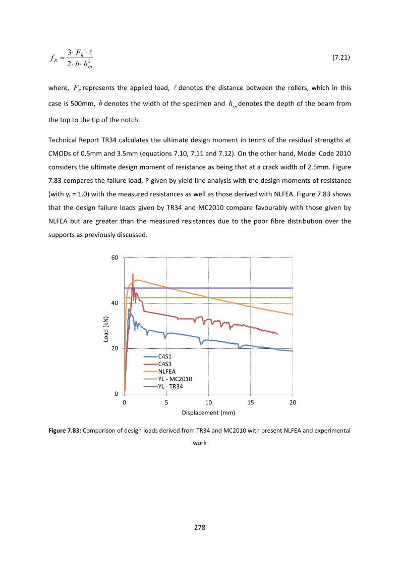
278
22
3
sp
RR
hb
Ff
(7.21)
where, RF represents the applied load, denotes the distance between the rollers, which in this
case is 500mm, b denotes the width of the specimen and sph denotes the depth of the beam from
the top to the tip of the notch.
Technical Report TR34 calculates the ultimate design moment in terms of the residual strengths at
CMODs of 0.5mm and 3.5mm (equations 7.10, 7.11 and 7.12). On the other hand, Model Code 2010
considers the ultimate design moment of resistance as being that at a crack width of 2.5mm. Figure
7.83 compares the failure load, P given by yield line analysis with the design moments of resistance
(with γc = 1.0) with the measured resistances as well as those derived with NLFEA. Figure 7.83 shows
that the design failure loads given by TR34 and MC2010 compare favourably with those given by
NLFEA but are greater than the measured resistances due to the poor fibre distribution over the
supports as previously discussed.
Figure 7.83: Comparison of design loads derived from TR34 and MC2010 with present NLFEA and experimental
work
0
20
40
60
0 5 10 15 20
Load
(kN
)
Displacement (mm)
C4S1 C4S3 NLFEA YL - MC2010 YL - TR34

279
7.6.8 Effect of additional restraint on the structural behaviour
Pile supported slabs are typically reinforced with fibre dosages of between 35 – 45 kg/m3 (The
Concrete Society, 2007). Incorporating such a dosage into a three point bending notched beam test
yields a tension softening response, as shown earlier in this research. From a design point of view, a
tension softening response is undesirable since it can lead to sudden failure without adequate
warning. In practice, SFRC pile supported slabs have been reported to develop a tension hardening
response (Thooft, 1999) (Destree, 2005).
Pile supported slabs commonly fail due to the folded plate and the circular fan mechanisms, as
described in Chapter Three. The load carrying capacity increases after initial micro cracking as the
fibres become activated. Subsequently, as the crack width increases there is a reduction in the load
being carried. If lateral restraint is present, membrane forces arise due to in plane restraint of the
lateral expansion that would otherwise arise following cracking (Eyre, 1994). These in plane
membrane forces are resisted by the axial restraint provided by the adjacent bays (Thooft, 1999)
(Nilsson, 2003) (Hedebratt & Silfwerbrand, 2004). Membrane forces arise due to in plane restraint of
the lateral expansion that would otherwise arise following cracking.
Rankin et al. (1997) presented a simple method based on deformation theory for predicting the
ultimate load capacity of laterally restrained reinforced concrete slabs. The method assumes an
elasto-plastic stress strain criterion. The load capacity from bending and compressive arching action
are calculated separately and then added to give the ultimate load capacity of the slab. The model
uses springs to model the effect of lateral restraint. A good correlation was reported between the
proposed method and previous empirical work.
Full scale experiments at Cardington by Peel Cross et al. (2001) were undertaken to assess the
contribution of compressive membrane action on the ultimate load capacity of interior, exterior and
corner panels in composite metal decking/concrete floor slabs. The interior panels exhibited 80%
higher strength than that calculated with yield line theory. This increase in load capacity has been
attributed to the comoressive membrane action occuring as a result of the lateral restraint. The
exterior and corner panel exhibited 51% and 47% respectively due to a lower contribution of axial
restraint.
Experimental research done by Nilson (2003) demonstrated the effect of the compressive arch
action on fibre reinforced sprayed concrete anchored in rock. Round slabs of various diameters were
loaded symmetrically which incorporated a fibre content of 30kg/m3. To simulate the effect of
compressive arch action, a steel ring was placed around some of the specimens. The aim of the work
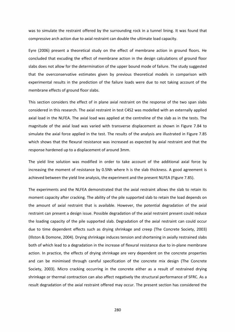
280
was to simulate the restraint offered by the surrounding rock in a tunnel lining. It was found that
compressive arch action due to axial restraint can double the ultimate load capacity.
Eyre (2006) present a theoretical study on the effect of membrane action in ground floors. He
concluded that excuding the effect of membrane action in the design calculations of ground floor
slabs does not allow for the determination of the upper bound mode of failure. The study suggested
that the overconservative estimates given by previous theoretical models in comparison with
experimental results in the prediction of the failure loads were due to not taking account of the
membrane effects of ground floor slabs.
This section considers the effect of in plane axial restraint on the response of the two span slabs
considered in this research. The axial restraint in test C4S2 was modelled with an externally applied
axial load in the NLFEA. The axial load was applied at the centreline of the slab as in the tests. The
magnitude of the axial load was varied with transverse displacement as shown in Figure 7.84 to
simulate the axial force applied in the test. The results of the analysis are illustrated in Figure 7.85
which shows that the flexural resistance was increased as expected by axial restraint and that the
response hardened up to a displacement of around 3mm.
The yield line solution was modified in order to take account of the additional axial force by
increasing the moment of resistance by 0.5Nh where h is the slab thickness. A good agreement is
achieved between the yield line analysis, the experiment and the present NLFEA (Figure 7.85).
The experiments and the NLFEA demonstrated that the axial restraint allows the slab to retain its
moment capacity after cracking. The ability of the pile supported slab to retain the load depends on
the amount of axial restraint that is available. However, the potential degradation of the axial
restraint can present a design issue. Possible degradation of the axial restraint present could reduce
the loading capacity of the pile supported slab. Degradation of the axial restraint can could occur
due to time dependent effects such as drying shrinkage and creep (The Concrete Society, 2003)
(Illston & Domone, 2004). Drying shrinkage induces tension and shortening in axially restrained slabs
both of which lead to a degradation in the increase of flexural resistance due to in-plane membrane
action. In practice, the effects of drying shrinkage are very dependent on the concrete properties
and can be minimised through careful specification of the concrete mix design (The Concrete
Society, 2003). Micro cracking occurring in the concrete either as a result of restrained drying
shrinkage or thermal contraction can also affect negatively the structural performance of SFRC. As a
result degradation of the axial restraint offered may occur. The present section has considered the

281
effect of axial restraint in the load deflection response of a SFRC slab. However, the subject of the
potential degradation of the axial force is beyond the scope of the present work.
Figure 7.84: Axial force versus vertical displacement
Figure 7.85: Effect of restraint on the load – deflection response of a two-span slab
0
10
20
30
0 2 4 6 8
Axi
al F
orc
e (k
N)
Displacement (mm)
Experiment
Yield Line
NLFEA
0
10
20
30
40
50
60
0 2 4 6 8 10
Load
(kN
)
Displacement (mm)
NLFEA
Yield Line
Experiment - C4S3
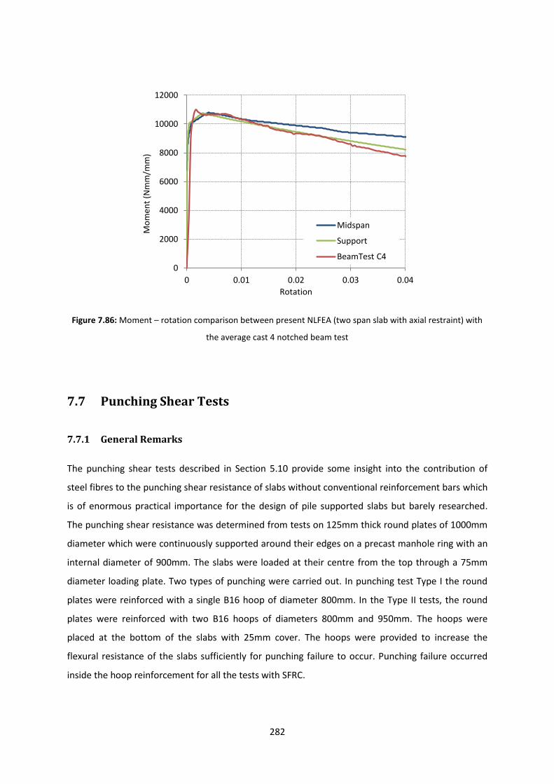
282
Figure 7.86: Moment – rotation comparison between present NLFEA (two span slab with axial restraint) with
the average cast 4 notched beam test
7.7 Punching Shear Tests
7.7.1 General Remarks
The punching shear tests described in Section 5.10 provide some insight into the contribution of
steel fibres to the punching shear resistance of slabs without conventional reinforcement bars which
is of enormous practical importance for the design of pile supported slabs but barely researched.
The punching shear resistance was determined from tests on 125mm thick round plates of 1000mm
diameter which were continuously supported around their edges on a precast manhole ring with an
internal diameter of 900mm. The slabs were loaded at their centre from the top through a 75mm
diameter loading plate. Two types of punching were carried out. In punching test Type I the round
plates were reinforced with a single B16 hoop of diameter 800mm. In the Type II tests, the round
plates were reinforced with two B16 hoops of diameters 800mm and 950mm. The hoops were
placed at the bottom of the slabs with 25mm cover. The hoops were provided to increase the
flexural resistance of the slabs sufficiently for punching failure to occur. Punching failure occurred
inside the hoop reinforcement for all the tests with SFRC.
0
2000
4000
6000
8000
10000
12000
0 0.01 0.02 0.03 0.04
Mo
men
t (N
mm
/mm
)
Rotation
Midspan
Support
BeamTest C4

283
7.6.2 Material Properties and Flexural Resistance
Self-compacting concrete was used with a compressive strength of 70MPa along with a fibre dosage
of 50kg/m3. The details of each of the four castings were described in Chapter Four and are provided
below for clarity:
Cast 1 was a plain concrete mix. This mix was used as a benchmark for assessing the effect of the
fibres.
In Cast 2, Arcelor Mittal He-75-35 steel fibres were added at a dosage of 50kg/m3. These are
35mm long hooked fibres with a 0.75mm diameter and an aspect ratio of 47. The tensile
strength of the fibres was 1200MPa.
Cast 3 incorporated Arcelor Mittal He-55-35 steel fibres at a dosage of 50kg/m3. These are
35mm long hooked fibres with a 0.55mm diameter and an aspect ratio of 64. The tensile
strength of the fibres was 1200MPa.
Cast 4 had Helix 5-25 fibres at a dosage of 50kg/m3. These are 25mm long twisted wire fibres
with a 0.5mm diameter and an aspect ratio of 50. The tensile strength of the fibres was
1700MPa.
The residual flexural strengths of the SFRC were estimated for each batch of three slabs from the
load displacement response of a RDP following the procedure outlined in Section 7.4.4. The initial
crack was assumed to form at a displacement of 1.4mm as this was the displacement at which the
plain concrete RDP failed. The complete set of load – deflection responses for these tests is given in
Section 5.10. The following equations were used to estimate the CMOD in terms of the central
displacements:
mmforCMOD 74.1575.0
(7.22)
mmforCMOD 746.0
(7.23)
Table 7.11 gives the displacements at the CMOD corresponding to the flexural strengths specified in
EN 14651 (British Standards Institution, 2005). Table 7.12 lists the peak loads measured in the RDP
tests as well as the loads at the displacements corresponding to CMOD of 0.5mm, 1.5mm, 2.5mm
and 3.5mm. The corresponding moments of resistance m in kNm/m, which were derived with yield
line analysis, and residual flexural strengths are given in Tables 7.13 and 7.14 respectively. The 4th
edition of the Concrete Society Report TR34 (The Concrete Society, 2012) gives the following
equation for the calculation of the plastic moment of resistance of SFRC slabs.
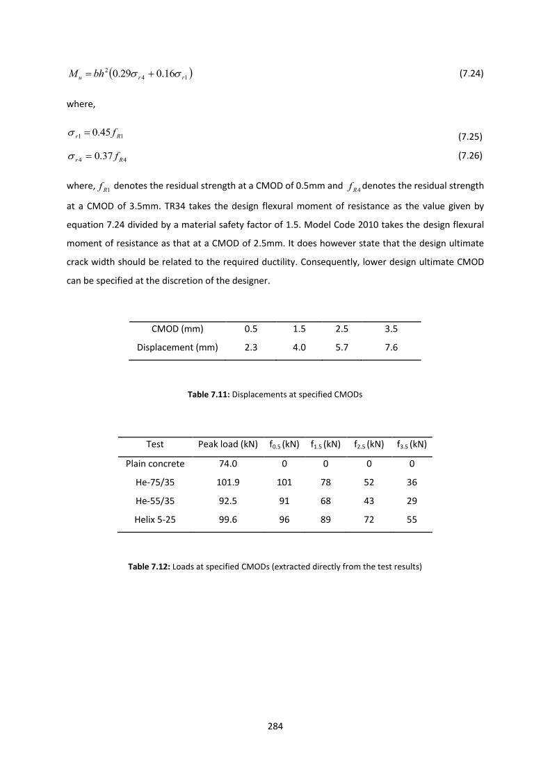
284
14
2 16.029.0 rru bhM
(7.24)
where,
11 45.0 Rr f
(7.25)
44 37.0 Rr f
(7.26)
where,1Rf denotes the residual strength at a CMOD of 0.5mm and
4Rf denotes the residual strength
at a CMOD of 3.5mm. TR34 takes the design flexural moment of resistance as the value given by
equation 7.24 divided by a material safety factor of 1.5. Model Code 2010 takes the design flexural
moment of resistance as that at a CMOD of 2.5mm. It does however state that the design ultimate
crack width should be related to the required ductility. Consequently, lower design ultimate CMOD
can be specified at the discretion of the designer.
CMOD (mm) 0.5 1.5 2.5 3.5
Displacement (mm) 2.3 4.0 5.7 7.6
Table 7.11: Displacements at specified CMODs
Test Peak load (kN) f0.5 (kN) f1.5 (kN) f2.5 (kN) f3.5 (kN)
Plain concrete 74.0 0 0 0 0
He-75/35 101.9 101 78 52 36
He-55/35 92.5 91 68 43 29
Helix 5-25 99.6 96 89 72 55
Table 7.12: Loads at specified CMODs (extracted directly from the test results)
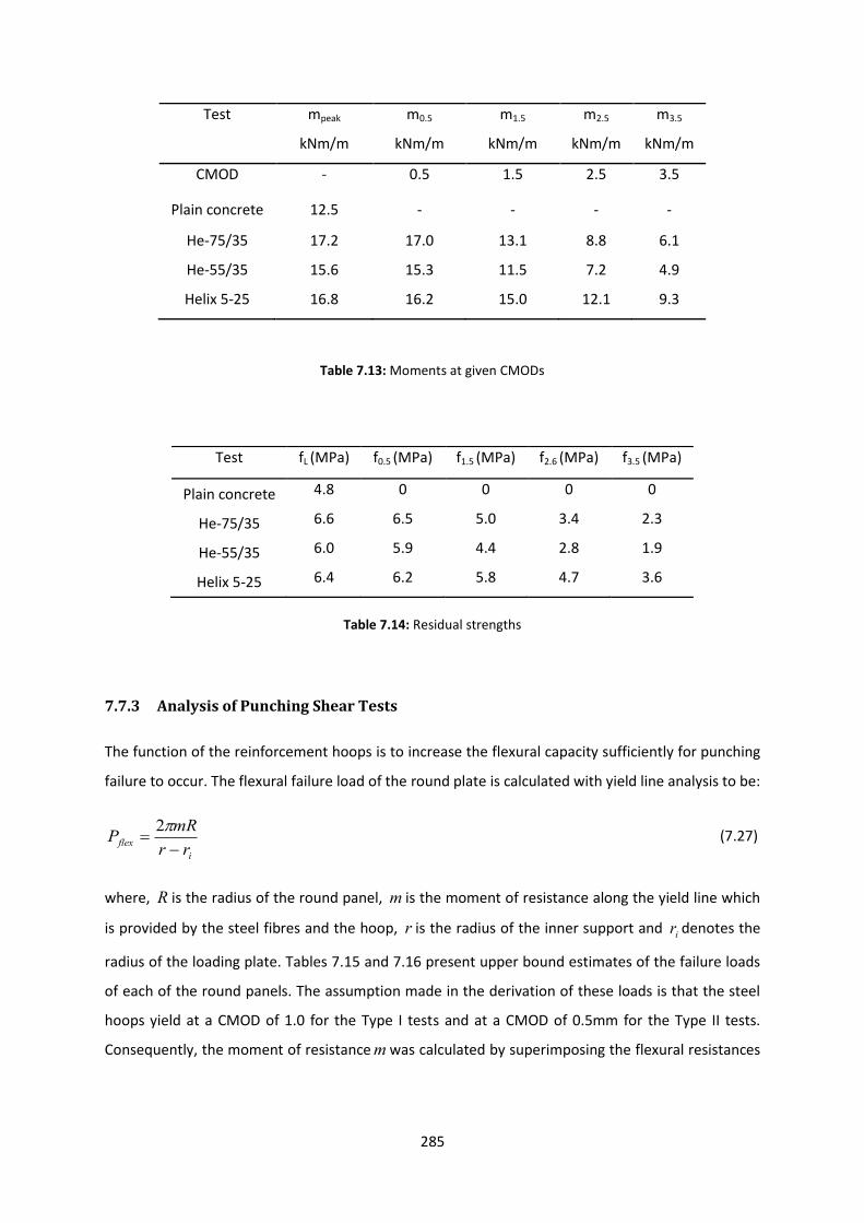
285
Test mpeak
kNm/m
m0.5
kNm/m
m1.5
kNm/m
m2.5
kNm/m
m3.5
kNm/m
CMOD - 0.5 1.5 2.5 3.5
Plain concrete 12.5 - - - -
He-75/35 17.2 17.0 13.1 8.8 6.1
He-55/35 15.6 15.3 11.5 7.2 4.9
Helix 5-25 16.8 16.2 15.0 12.1 9.3
Table 7.13: Moments at given CMODs
Table 7.14: Residual strengths
7.7.3 Analysis of Punching Shear Tests
The function of the reinforcement hoops is to increase the flexural capacity sufficiently for punching
failure to occur. The flexural failure load of the round plate is calculated with yield line analysis to be:
i
flexrr
mRP
2 (7.27)
where, R is the radius of the round panel, m is the moment of resistance along the yield line which
is provided by the steel fibres and the hoop, r is the radius of the inner support and ir denotes the
radius of the loading plate. Tables 7.15 and 7.16 present upper bound estimates of the failure loads
of each of the round panels. The assumption made in the derivation of these loads is that the steel
hoops yield at a CMOD of 1.0 for the Type I tests and at a CMOD of 0.5mm for the Type II tests.
Consequently, the moment of resistancemwas calculated by superimposing the flexural resistances
Test fL (MPa) f0.5 (MPa) f1.5 (MPa) f2.6 (MPa) f3.5 (MPa)
Plain concrete 4.8 0 0 0 0
He-75/35 6.6 6.5 5.0 3.4 2.3
He-55/35 6.0 5.9 4.4 2.8 1.9
Helix 5-25 6.4 6.2 5.8 4.7 3.6
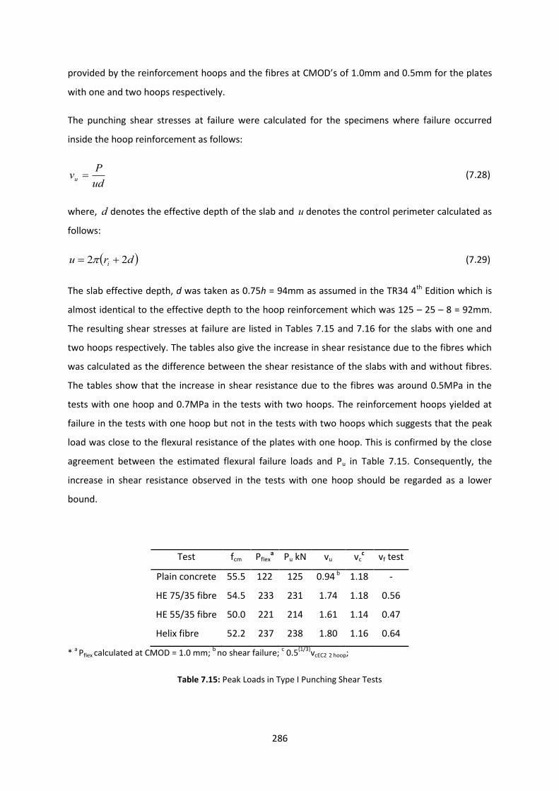
286
provided by the reinforcement hoops and the fibres at CMOD’s of 1.0mm and 0.5mm for the plates
with one and two hoops respectively.
The punching shear stresses at failure were calculated for the specimens where failure occurred
inside the hoop reinforcement as follows:
ud
Pvu (7.28)
where, d denotes the effective depth of the slab and u denotes the control perimeter calculated as
follows:
dru i 22 (7.29)
The slab effective depth, d was taken as 0.75h = 94mm as assumed in the TR34 4th Edition which is
almost identical to the effective depth to the hoop reinforcement which was 125 – 25 – 8 = 92mm.
The resulting shear stresses at failure are listed in Tables 7.15 and 7.16 for the slabs with one and
two hoops respectively. The tables also give the increase in shear resistance due to the fibres which
was calculated as the difference between the shear resistance of the slabs with and without fibres.
The tables show that the increase in shear resistance due to the fibres was around 0.5MPa in the
tests with one hoop and 0.7MPa in the tests with two hoops. The reinforcement hoops yielded at
failure in the tests with one hoop but not in the tests with two hoops which suggests that the peak
load was close to the flexural resistance of the plates with one hoop. This is confirmed by the close
agreement between the estimated flexural failure loads and Pu in Table 7.15. Consequently, the
increase in shear resistance observed in the tests with one hoop should be regarded as a lower
bound.
Test fcm Pflexa Pu kN vu vc
c vf test
Plain concrete 55.5 122 125 0.94 b 1.18 -
HE 75/35 fibre 54.5 233 231 1.74 1.18 0.56
HE 55/35 fibre 50.0 221 214 1.61 1.14 0.47
Helix fibre 52.2 237 238 1.80 1.16 0.64
* a
Pflex calculated at CMOD = 1.0 mm; b
no shear failure; c 0.5
(1/3)vcEC2 2 hoop;
Table 7.15: Peak Loads in Type I Punching Shear Tests
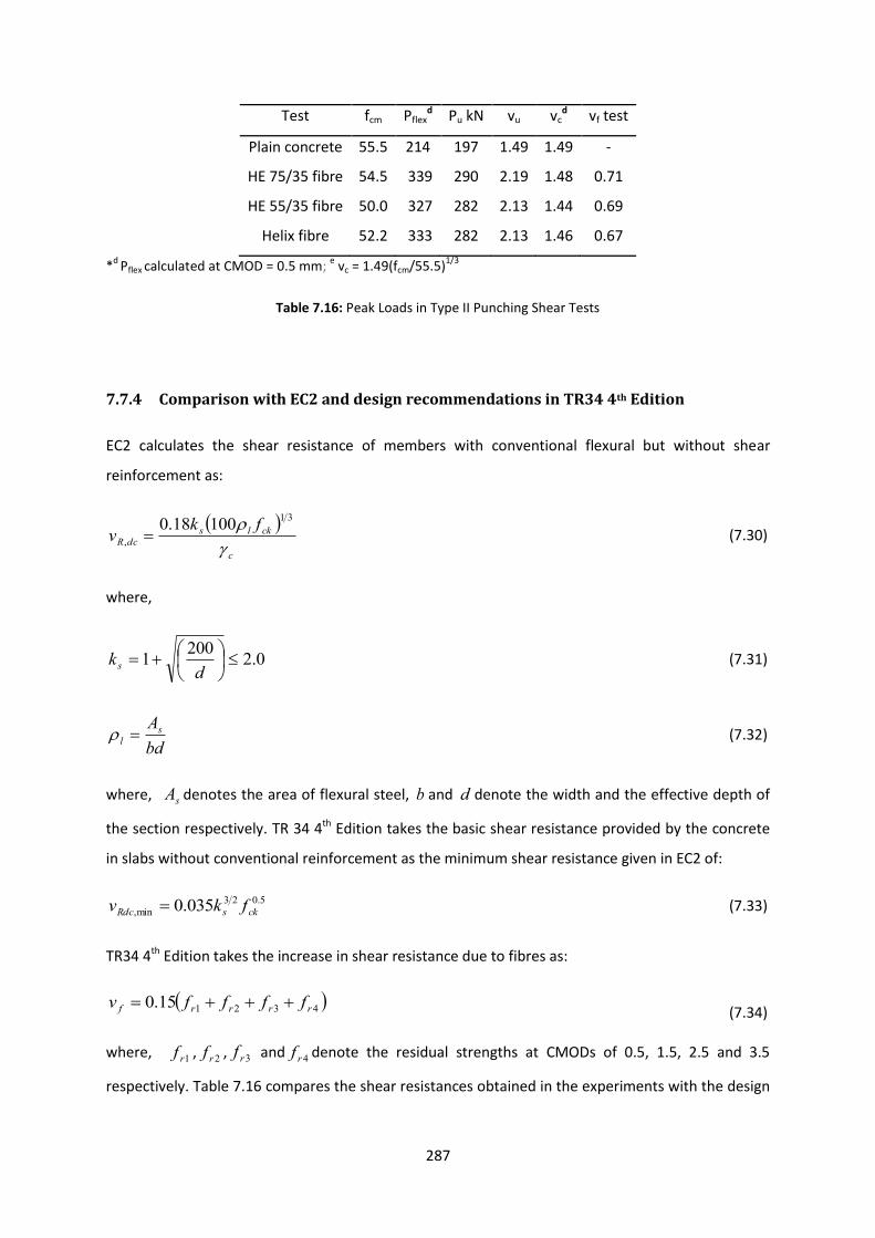
287
Test fcm Pflexd Pu kN vu vc
d vf test
Plain concrete 55.5 214 197 1.49 1.49 -
HE 75/35 fibre 54.5 339 290 2.19 1.48 0.71
HE 55/35 fibre 50.0 327 282 2.13 1.44 0.69
Helix fibre 52.2 333 282 2.13 1.46 0.67
*d
Pflex calculated at CMOD = 0.5 mm; e vc = 1.49(fcm/55.5)
1/3
Table 7.16: Peak Loads in Type II Punching Shear Tests
7.7.4 Comparison with EC2 and design recommendations in TR34 4th Edition
EC2 calculates the shear resistance of members with conventional flexural but without shear
reinforcement as:
c
ckls
dcR
fkv
31
,
10018.0 (7.30)
where,
0.2200
1
dks (7.31)
bd
Asl (7.32)
where, sA denotes the area of flexural steel, b and d denote the width and the effective depth of
the section respectively. TR 34 4th Edition takes the basic shear resistance provided by the concrete
in slabs without conventional reinforcement as the minimum shear resistance given in EC2 of:
5.023
min, 035.0 cksRdc fkv (7.33)
TR34 4th Edition takes the increase in shear resistance due to fibres as:
432115.0 rrrrf ffffv (7.34)
where, 1rf , 2rf , 3rf and 4rf denote the residual strengths at CMODs of 0.5, 1.5, 2.5 and 3.5
respectively. Table 7.16 compares the shear resistances obtained in the experiments with the design
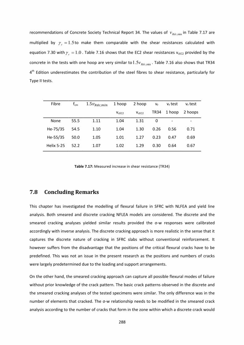
288
recommendations of Concrete Society Technical Report 34. The values of min,Rdcv in Table 7.17 are
multiplied by 5.1c to make them comparable with the shear resistances calculated with
equation 7.30 with 0.1c . Table 7.16 shows that the EC2 shear resistances vcEC2 provided by the
concrete in the tests with one hoop are very similar to min,5.1 Rdcv . Table 7.16 also shows that TR34
4th Edition underestimates the contribution of the steel fibres to shear resistance, particularly for
Type II tests.
Fibre fcm 1 hoop
vcEC2
2 hoop
vcEC2
vf
TR34
vf test
1 hoop
vf test
2 hoops
None 55.5 1.11 1.04 1.31 0 - -
He-75/35 54.5 1.10 1.04 1.30 0.26 0.56 0.71
He-55/35 50.0 1.05 1.01 1.27 0.23 0.47 0.69
Helix 5-25 52.2 1.07 1.02 1.29 0.30 0.64 0.67
Table 7.17: Measured increase in shear resistance (TR34)
7.8 Concluding Remarks
This chapter has investigated the modelling of flexural failure in SFRC with NLFEA and yield line
analysis. Both smeared and discrete cracking NFLEA models are considered. The discrete and the
smeared cracking analyses yielded similar results provided the σ-w responses were calibrated
accordingly with inverse analysis. The discrete cracking approach is more realistic in the sense that it
captures the discrete nature of cracking in SFRC slabs without conventional reinforcement. It
however suffers from the disadvantage that the positions of the critical flexural cracks have to be
predefined. This was not an issue in the present research as the positions and numbers of cracks
were largely predetermined due to the loading and support arrangements.
On the other hand, the smeared cracking approach can capture all possible flexural modes of failure
without prior knowledge of the crack pattern. The basic crack patterns observed in the discrete and
the smeared cracking analyses of the tested specimens were similar. The only difference was in the
number of elements that cracked. The σ-w relationship needs to be modified in the smeared crack
analysis according to the number of cracks that form in the zone within which a discrete crack would
289
form in reality. The actual crack width can be estimated as the sum of the crack widths in the
cracked elements within the fracture zone that would in reality consist of a single discrete crack. The
smeared cracking approach can also be used as a preliminary design tool in order to identify the
location of the cracks for input into a discrete crack analysis.
The experimental results obtained from the round plate and two span slab tests indicated a softer
approach than expected from the notched beam tests. NLFEA has the advantage of providing
information on the elastic response of the slabs unlike the yield line method. This is useful for
assessing the complete response of SFRC slabs but comes at a price at large computational cost. In
addition, the yield line method does not provide any information regarding the sequence crack
formation as it considers the slab to be fully cracked from first loading. The complexity of NLFEA
makes it unsuitable as a design tool unlike yield line analysis which gives good results and is
relatively straightforward to implement.
The average displacement – CMOD responses of the RDP were consistent despite the differences
observed in the crack pattern. Using the equations proposed for the calculation of the CMOD from
the displacement showed a very good agreement with the corresponding experimental values. The
average residual strengths obtained from the notched beams are greater than the ones obtained
from the RDP. This difference arises since the beam doesn’t fail at its weakest position due to the
incorporation of the notch. The ultimate moment capacities predicted by the Technical Report 34
(The Concrete Society, 2012) and the Model Code 2010 (International Federation for Structural
Concrete, 2010) were compared to the experimental values. They were found to give conservative
estimates of the design moment of resistance. Model Code 2010 gives more conservative results to
Technical Report 34 when then the design moment of resistance is calculated at a CMOD of 2.5mm
as recommended.
The yield line analysis results for the two span slab were comparable with those of the NLFEA. The
experimental results however did not show a particularly good correspondence due to the poor fibre
distribution observed in the tests. The two span slab experiments demonstrated that a hardening
response can develop in slabs cast from tension softening SFRC provided sufficient axial restraint is
available as can be the case in practice. In the punching shear tests, the increase in shear resistance
due to the addition of the steel fibres was 0.5MPa for the Type I tests (one hoop) and 0.7MPa for the
Type II tests (two hoops) respectively. The recommendations of Technical Report 34 were found to
underestimate the contribution of the steel fibres to the punching shear resistance especially the
shear tests reinforced with two hoops (Type II tests).
290
Chapter Eight
Analysis of Pile Supported Slabs
8.1 General Remarks
Chapter 7 considered the analysis of the tested slabs using NLFEA and yield line analysis. This
chapter examines the analysis of SFRC pile-supported slabs using NLFEA. Particular emphasis is
placed on determining the changes in the moment distribution along cracks as the slab is loaded to
failure. Both discrete and smeared cracking approaches are considered.
8.2 Discrete Cracking Approach
8.2.1 General modelling considerations
The present section explains the modelling procedure adopted and presents results of simulations of
flexural failure in the internal panel of a pile supported slab.
A single internal bay is modelled of dimensions 1500mm x 1500mm. The thickness of the slab has
been chosen as 125mm in order to match the thicknesses of the notched beam, RDP and slab tests
undertaken. To reduce the computation time of each analysis a quarter of the bay has been
modelled taking advantage of symmetry (Figure 8.1).
The loading on the slabs has been simulated by applying a displacement at the centre of the quarter
panel. In order to force the elements along the yield lines to crack, the tensile strength of the other
elements was increased. As explained in Chapter Seven, NLFEA gives the complete flexural response
from first loading to failure and the distribution of bending moment along cracks unlike yield line
analysis. The yield line analysis for this mechanism is presented in Section 3.4. Both yield line
analysis and discrete crack formulations, as presented in this thesis, suffer from the drawback that
the crack pattern has to be assumed in advance though there are ways round this which are beyond
the scope of this thesis. In the present work, the piles are assumed to be sufficiently large that the
fan mechanism is not critical. The slab was modelled with four-noded square elements with reduced
integration using the mesh shown in Figure 8.2 in which the elements measure 20mm square.
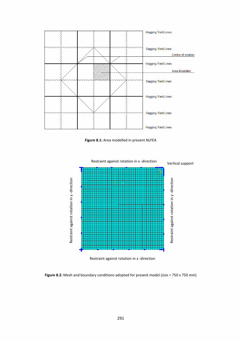
291
Figure 8.1: Area modelled in present NLFEA
Figure 8.2: Mesh and boundary conditions adopted for present model (size = 750 x 750 mm)
Restraint against rotation in x -direction
Restraint against rotation in x -direction
Res
trai
nt
agai
nst
ro
tati
on
in y
-d
irec
tio
n
Res
trai
nt
agai
nst
ro
tati
on
in y
-d
irec
tio
n
Vertical support
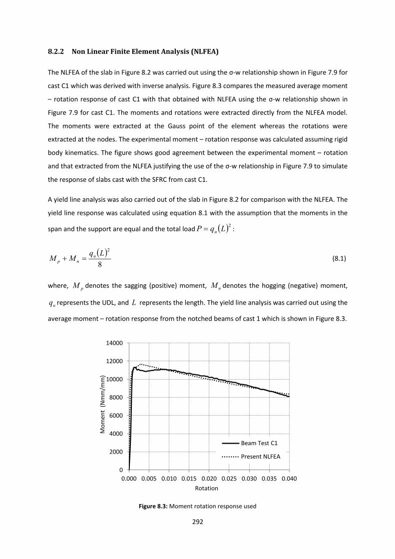
292
8.2.2 Non Linear Finite Element Analysis (NLFEA)
The NLFEA of the slab in Figure 8.2 was carried out using the σ-w relationship shown in Figure 7.9 for
cast C1 which was derived with inverse analysis. Figure 8.3 compares the measured average moment
– rotation response of cast C1 with that obtained with NLFEA using the σ-w relationship shown in
Figure 7.9 for cast C1. The moments and rotations were extracted directly from the NLFEA model.
The moments were extracted at the Gauss point of the element whereas the rotations were
extracted at the nodes. The experimental moment – rotation response was calculated assuming rigid
body kinematics. The figure shows good agreement between the experimental moment – rotation
and that extracted from the NLFEA justifying the use of the σ-w relationship in Figure 7.9 to simulate
the response of slabs cast with the SFRC from cast C1.
A yield line analysis was also carried out of the slab in Figure 8.2 for comparison with the NLFEA. The
yield line response was calculated using equation 8.1 with the assumption that the moments in the
span and the support are equal and the total load 2LqP u :
8
2Lq
MM u
np (8.1)
where, pM denotes the sagging (positive) moment, nM denotes the hogging (negative) moment,
uq represents the UDL, and L represents the length. The yield line analysis was carried out using the
average moment – rotation response from the notched beams of cast 1 which is shown in Figure 8.3.
Figure 8.3: Moment rotation response used
0
2000
4000
6000
8000
10000
12000
14000
0.000 0.005 0.010 0.015 0.020 0.025 0.030 0.035 0.040
Mo
men
t (
Nm
m/m
m)
Rotation
Beam Test C1
Present NLFEA
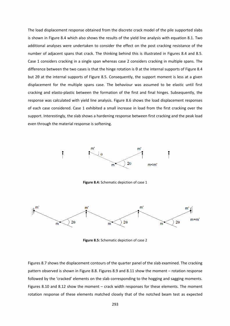
293
The load displacement response obtained from the discrete crack model of the pile supported slabs
is shown in Figure 8.4 which also shows the results of the yield line analysis with equation 8.1. Two
additional analyses were undertaken to consider the effect on the post cracking resistance of the
number of adjacent spans that crack. The thinking behind this is illustrated in Figures 8.4 and 8.5.
Case 1 considers cracking in a single span whereas case 2 considers cracking in multiple spans. The
difference between the two cases is that the hinge rotation is θ at the internal supports of Figure 8.4
but 2θ at the internal supports of Figure 8.5. Consequently, the support moment is less at a given
displacement for the multiple spans case. The behaviour was assumed to be elastic until first
cracking and elasto-plastic between the formation of the first and final hinges. Subsequently, the
response was calculated with yield line analysis. Figure 8.6 shows the load displacement responses
of each case considered. Case 1 exhibited a small increase in load from the first cracking over the
support. Interestingly, the slab shows a hardening response between first cracking and the peak load
even through the material response is softening.
Figure 8.4: Schematic depiction of case 1
Figure 8.5: Schematic depiction of case 2
Figures 8.7 shows the displacement contours of the quarter panel of the slab examined. The cracking
pattern observed is shown in Figure 8.8. Figures 8.9 and 8.11 show the moment – rotation response
followed by the ‘cracked’ elements on the slab corresponding to the hogging and sagging moments.
Figures 8.10 and 8.12 show the moment – crack width responses for these elements. The moment
rotation response of these elements matched closely that of the notched beam test as expected
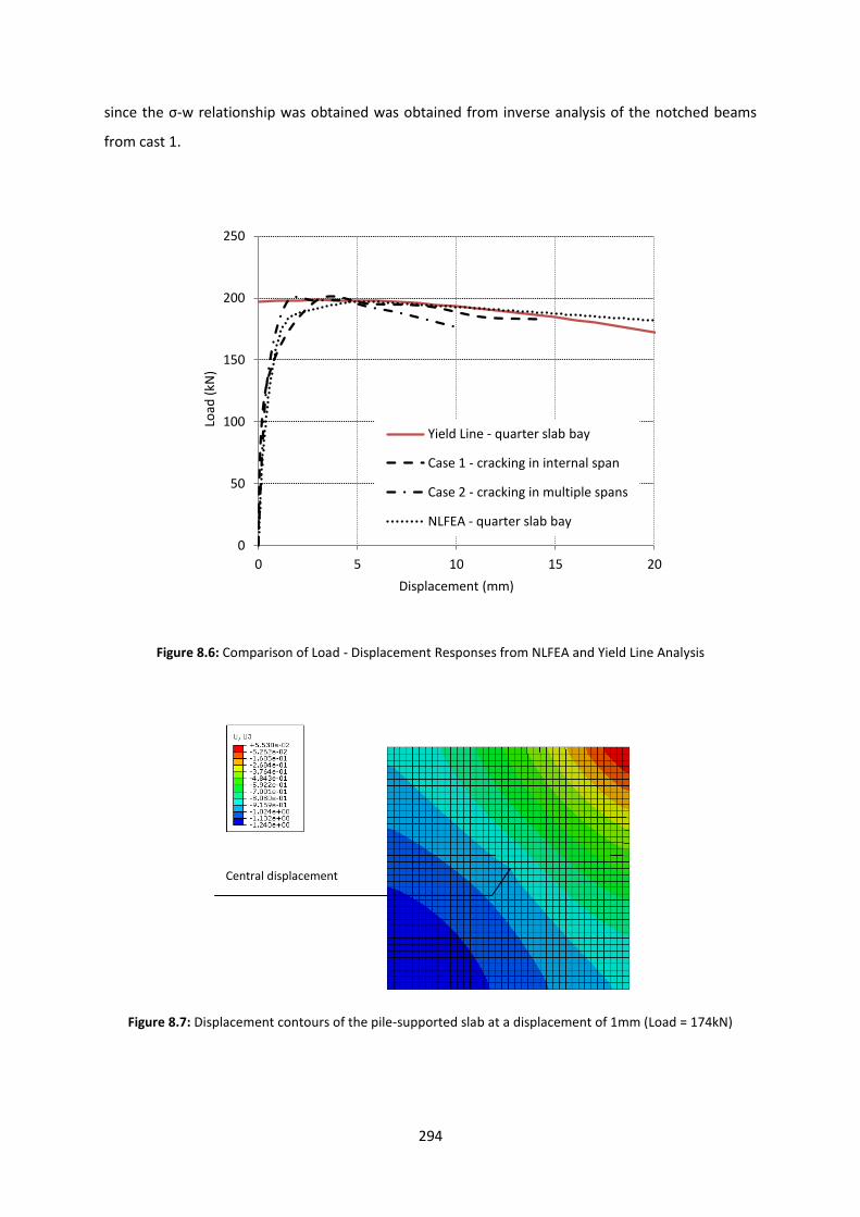
294
since the σ-w relationship was obtained was obtained from inverse analysis of the notched beams
from cast 1.
Figure 8.6: Comparison of Load - Displacement Responses from NLFEA and Yield Line Analysis
Figure 8.7: Displacement contours of the pile-supported slab at a displacement of 1mm (Load = 174kN)
0
50
100
150
200
250
0 5 10 15 20
Load
(kN
)
Displacement (mm)
Yield Line - quarter slab bay
Case 1 - cracking in internal span
Case 2 - cracking in multiple spans
NLFEA - quarter slab bay
Central displacement
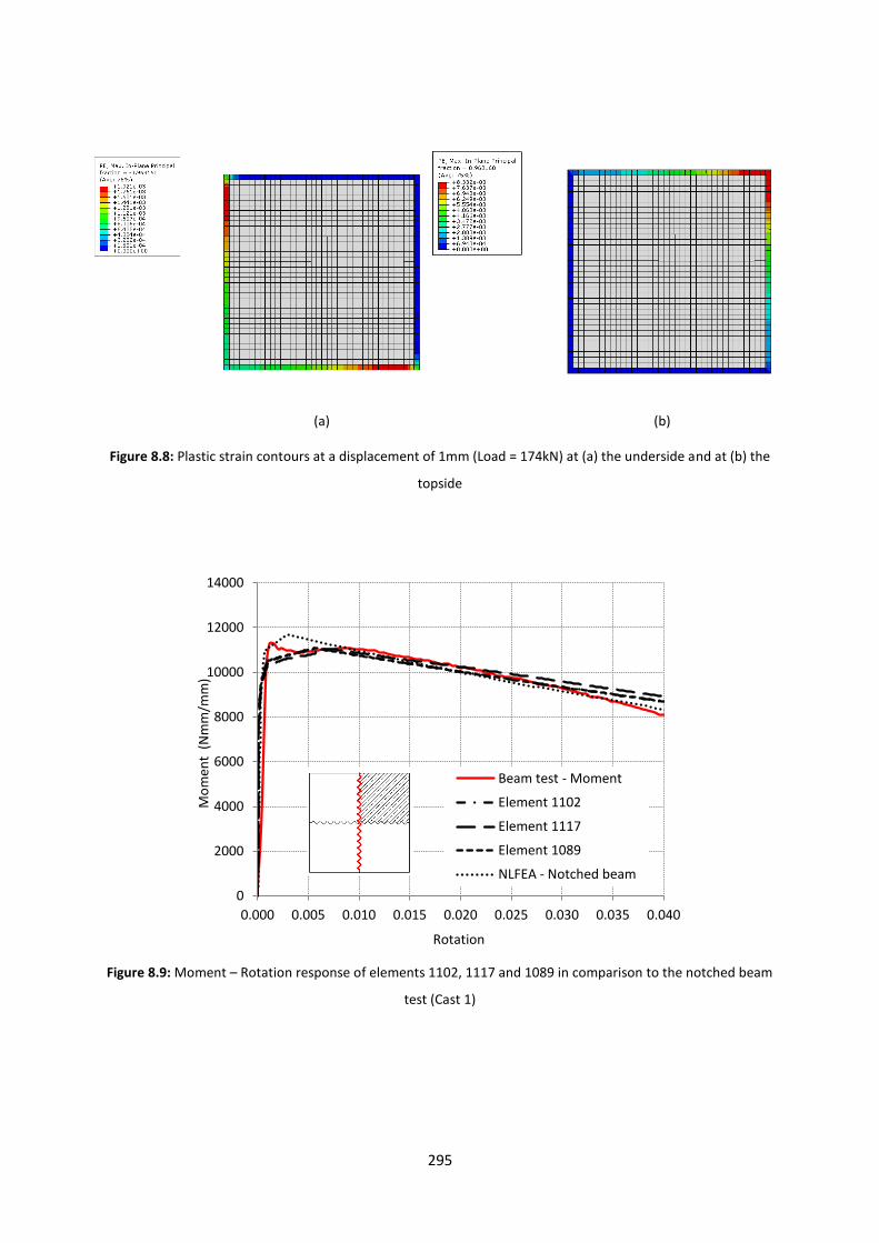
295
(a) (b)
Figure 8.8: Plastic strain contours at a displacement of 1mm (Load = 174kN) at (a) the underside and at (b) the
topside
Figure 8.9: Moment – Rotation response of elements 1102, 1117 and 1089 in comparison to the notched beam
test (Cast 1)
0
2000
4000
6000
8000
10000
12000
14000
0.000 0.005 0.010 0.015 0.020 0.025 0.030 0.035 0.040
Mo
men
t (
Nm
m/m
m)
Rotation
Beam test - Moment
Element 1102
Element 1117
Element 1089
NLFEA - Notched beam
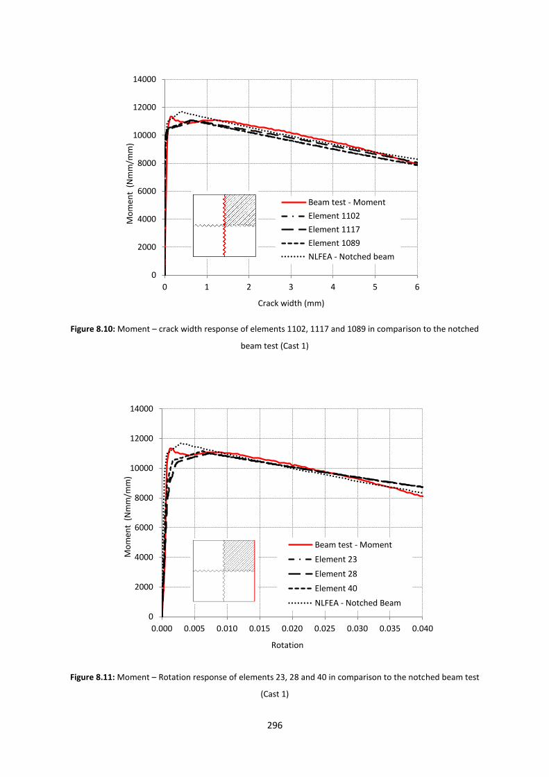
296
Figure 8.10: Moment – crack width response of elements 1102, 1117 and 1089 in comparison to the notched
beam test (Cast 1)
Figure 8.11: Moment – Rotation response of elements 23, 28 and 40 in comparison to the notched beam test
(Cast 1)
0
2000
4000
6000
8000
10000
12000
14000
0 1 2 3 4 5 6
Mo
men
t (
Nm
m/m
m)
Crack width (mm)
Beam test - Moment
Element 1102
Element 1117
Element 1089
NLFEA - Notched beam
0
2000
4000
6000
8000
10000
12000
14000
0.000 0.005 0.010 0.015 0.020 0.025 0.030 0.035 0.040
Mo
men
t (
Nm
m/m
m)
Rotation
Beam test - Moment
Element 23
Element 28
Element 40
NLFEA - Notched Beam
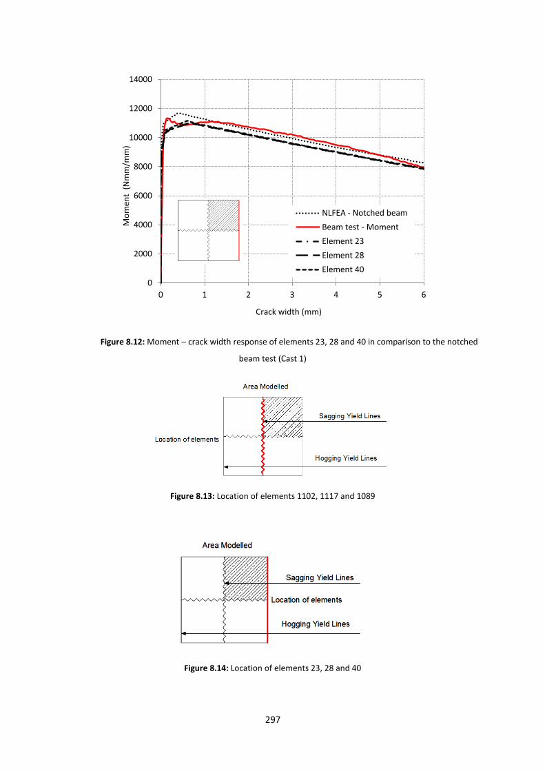
297
Figure 8.12: Moment – crack width response of elements 23, 28 and 40 in comparison to the notched
beam test (Cast 1)
Figure 8.13: Location of elements 1102, 1117 and 1089
Figure 8.14: Location of elements 23, 28 and 40
0
2000
4000
6000
8000
10000
12000
14000
0 1 2 3 4 5 6
Mo
men
t (
Nm
m/m
m)
Crack width (mm)
NLFEA - Notched beam
Beam test - Moment
Element 23
Element 28
Element 40
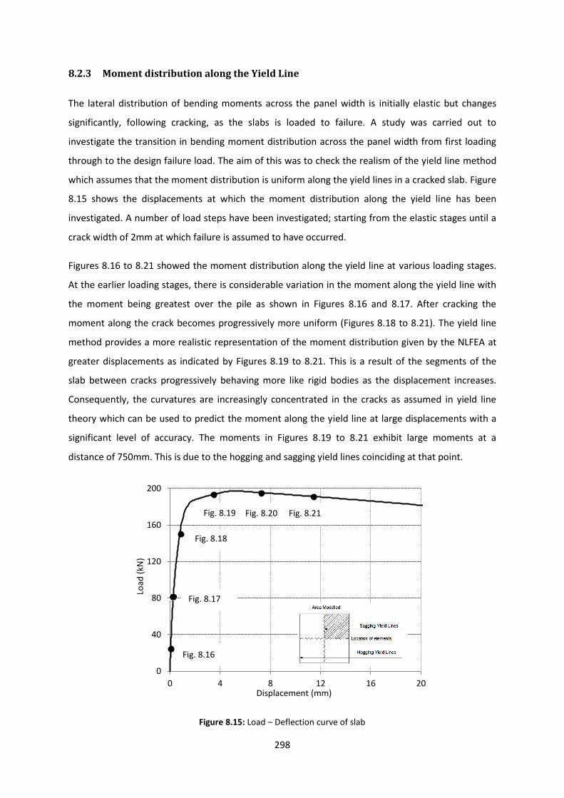
298
8.2.3 Moment distribution along the Yield Line
The lateral distribution of bending moments across the panel width is initially elastic but changes
significantly, following cracking, as the slabs is loaded to failure. A study was carried out to
investigate the transition in bending moment distribution across the panel width from first loading
through to the design failure load. The aim of this was to check the realism of the yield line method
which assumes that the moment distribution is uniform along the yield lines in a cracked slab. Figure
8.15 shows the displacements at which the moment distribution along the yield line has been
investigated. A number of load steps have been investigated; starting from the elastic stages until a
crack width of 2mm at which failure is assumed to have occurred.
Figures 8.16 to 8.21 showed the moment distribution along the yield line at various loading stages.
At the earlier loading stages, there is considerable variation in the moment along the yield line with
the moment being greatest over the pile as shown in Figures 8.16 and 8.17. After cracking the
moment along the crack becomes progressively more uniform (Figures 8.18 to 8.21). The yield line
method provides a more realistic representation of the moment distribution given by the NLFEA at
greater displacements as indicated by Figures 8.19 to 8.21. This is a result of the segments of the
slab between cracks progressively behaving more like rigid bodies as the displacement increases.
Consequently, the curvatures are increasingly concentrated in the cracks as assumed in yield line
theory which can be used to predict the moment along the yield line at large displacements with a
significant level of accuracy. The moments in Figures 8.19 to 8.21 exhibit large moments at a
distance of 750mm. This is due to the hogging and sagging yield lines coinciding at that point.
Figure 8.15: Load – Deflection curve of slab
0
40
80
120
160
200
0 4 8 12 16 20
Load
(kN
)
Displacement (mm)
Fig. 8.17
Fig. 8.18
Fig. 8.19 Fig. 8.20 Fig. 8.21
Fig. 8.16
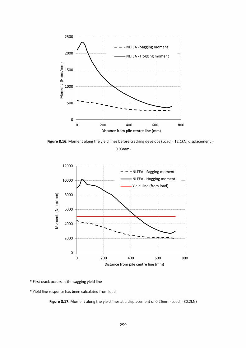
299
Figure 8.16: Moment along the yield lines before cracking develops (Load = 12.1kN, displacement =
0.03mm)
* First crack occurs at the sagging yield line
* Yield line response has been calculated from load
Figure 8.17: Moment along the yield lines at a displacement of 0.26mm (Load = 80.2kN)
0
500
1000
1500
2000
2500
0 200 400 600 800
Mo
men
t (
Nm
m/m
m)
Distance from pile centre line (mm)
NLFEA - Sagging moment
NLFEA - Hogging moment
0
2000
4000
6000
8000
10000
12000
0 200 400 600 800
Mo
men
t (
Nm
m/m
m)
Distance from pile centre line (mm)
NLFEA - Sagging moment
NLFEA - Hogging moment
Yield Line (from load)
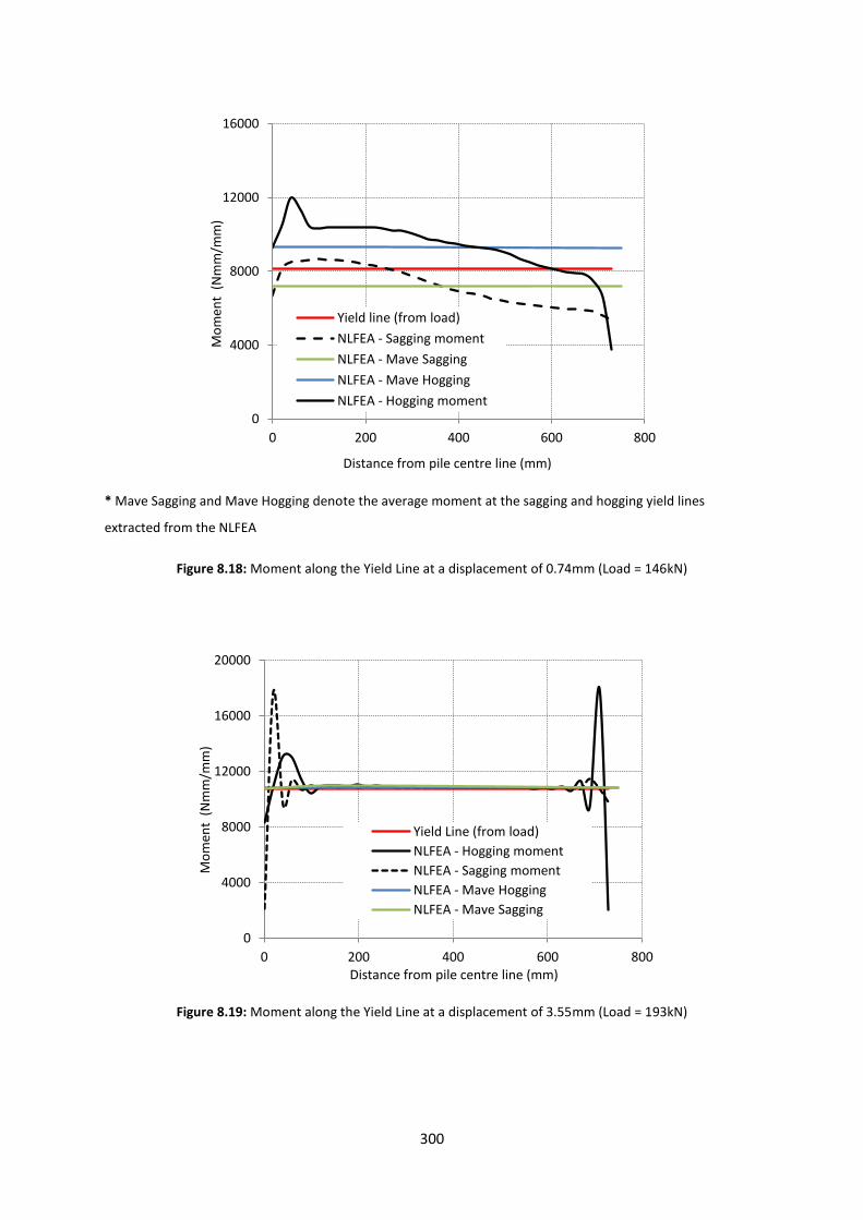
300
* Mave Sagging and Mave Hogging denote the average moment at the sagging and hogging yield lines
extracted from the NLFEA
Figure 8.18: Moment along the Yield Line at a displacement of 0.74mm (Load = 146kN)
Figure 8.19: Moment along the Yield Line at a displacement of 3.55mm (Load = 193kN)
0
4000
8000
12000
16000
0 200 400 600 800
Mo
men
t (
Nm
m/m
m)
Distance from pile centre line (mm)
Yield line (from load)
NLFEA - Sagging moment
NLFEA - Mave Sagging
NLFEA - Mave Hogging
NLFEA - Hogging moment
0
4000
8000
12000
16000
20000
0 200 400 600 800
Mo
men
t (
Nm
m/m
m)
Distance from pile centre line (mm)
Yield Line (from load)
NLFEA - Hogging moment
NLFEA - Sagging moment
NLFEA - Mave Hogging
NLFEA - Mave Sagging
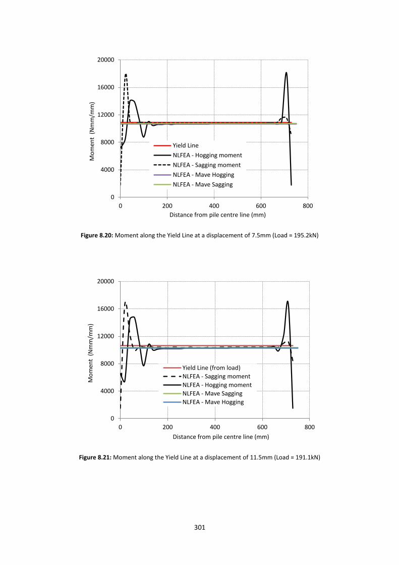
301
Figure 8.20: Moment along the Yield Line at a displacement of 7.5mm (Load = 195.2kN)
Figure 8.21: Moment along the Yield Line at a displacement of 11.5mm (Load = 191.1kN)
0
4000
8000
12000
16000
20000
0 200 400 600 800
Mo
men
t (
Nm
m/m
m)
Distance from pile centre line (mm)
Yield Line
NLFEA - Hogging moment
NLFEA - Sagging moment
NLFEA - Mave Hogging
NLFEA - Mave Sagging
0
4000
8000
12000
16000
20000
0 200 400 600 800
Mo
men
t (
Nm
m/m
m)
Distance from pile centre line (mm)
Yield Line (from load)
NLFEA - Sagging moment
NLFEA - Hogging moment
NLFEA - Mave Sagging
NLFEA - Mave Hogging

302
8.2.4 Rotation along the Yield Line
This section compares the rotations and crack widths along the yield lines extracted from the NLFEA
with those calculated assuming rigid body kinematics. The purpose of the exercise was to gain some
insight into the accuracy of the assumptions implicit in a yield line analysis of a typical pile supported
slab. The rotations and crack widths were extracted from the NLFEA at the same displacements as
the moments in Figures 8.18 to 8.21 (i.e. at displacements of 0.74mm, 3.55mm, 7.5mm and
11.5mm). The results are shown in Figures 8.22, 8.24, 8.26 and 8.28 which show the rotations along
the sagging and hogging yield line as well as the rotations calculated assuming rigid body kinematics.
Figures 8.23, 8.25, 8.27 and 8.29 show the crack widths derived from the NLFEA as well as the
corresponding crack widths calculated from rigid body kinematics.
Before first cracking, the structure behaves elastically. At the onset of cracking there is some elastic
deformation. However, the slab does not behave as a completely rigid body. Hence, one can observe
some differences between the actual and predicted rotations in Figure 8.22. Figures 8.23 and 8.25
show that the crack width along the yield line varies, with the greatest crack widths occurring over
the pile as expected. As the displacement increases, the elastic rotations of the slab become
increasingly insignificant and as a result the crack widths given by the NLFEA converge towards those
given by rigid body kinematics as shown in Figures 8.26 to 8.29.
Consequently, at larger displacements, the crack widths become more uniform over the yield line as
shown in Figures 8.27 and 8.29. As a result of the reduced significance of the elastic deformation,
the crack width predictions from the yield line become increasingly comparable with increasing
displacement to those obtained from the NLFEA. In the limit, the crack widths from the yield line
method and the NLFEA would converge, as the elastic deformations comprise a very small
percentage of the total deformation at large displacements.
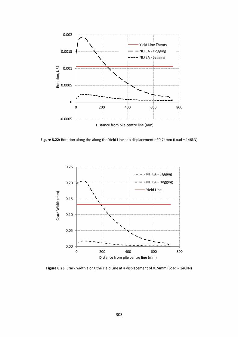
303
Figure 8.22: Rotation along the along the Yield Line at a displacement of 0.74mm (Load = 146kN)
Figure 8.23: Crack width along the Yield Line at a displacement of 0.74mm (Load = 146kN)
-0.0005
0
0.0005
0.001
0.0015
0.002
0 200 400 600 800
Ro
tati
on
, UR
1
Distance from pile centre line (mm)
Yield Line Theory
NLFEA - Hogging
NLFEA - Sagging
0.00
0.05
0.10
0.15
0.20
0.25
0 200 400 600 800
Cra
ck W
idth
(m
m)
Distance from pile centre line (mm)
NLFEA - Sagging
NLFEA - Hogging
Yield Line
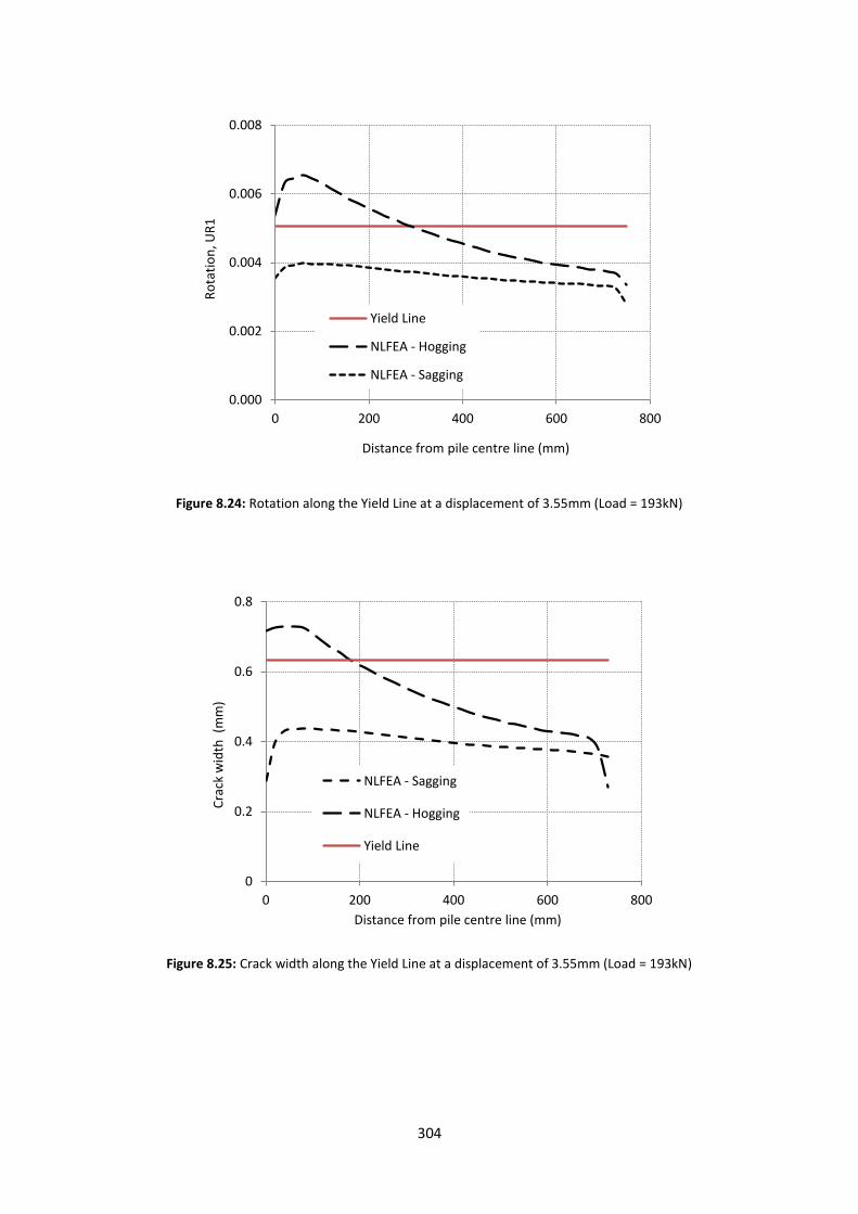
304
Figure 8.24: Rotation along the Yield Line at a displacement of 3.55mm (Load = 193kN)
Figure 8.25: Crack width along the Yield Line at a displacement of 3.55mm (Load = 193kN)
0.000
0.002
0.004
0.006
0.008
0 200 400 600 800
Ro
tati
on
, UR
1
Distance from pile centre line (mm)
Yield Line
NLFEA - Hogging
NLFEA - Sagging
0
0.2
0.4
0.6
0.8
0 200 400 600 800
Cra
ck w
idth
(m
m)
Distance from pile centre line (mm)
NLFEA - Sagging
NLFEA - Hogging
Yield Line
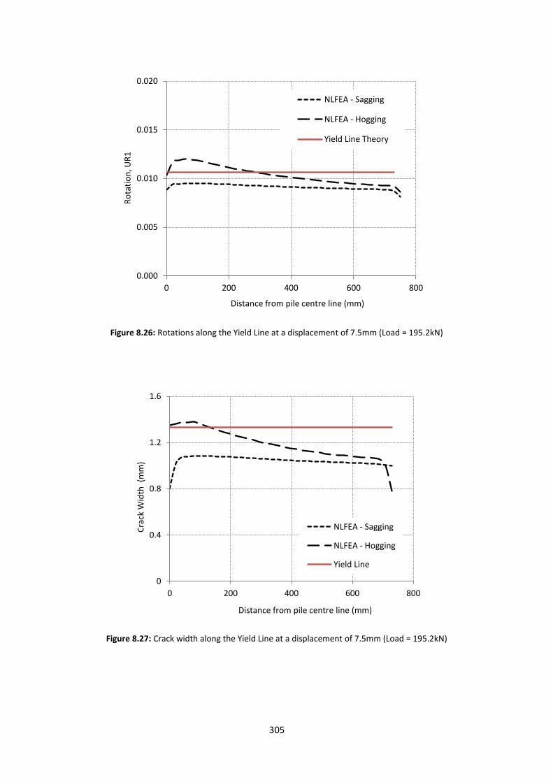
305
Figure 8.26: Rotations along the Yield Line at a displacement of 7.5mm (Load = 195.2kN)
Figure 8.27: Crack width along the Yield Line at a displacement of 7.5mm (Load = 195.2kN)
0.000
0.005
0.010
0.015
0.020
0 200 400 600 800
Ro
tati
on
, UR
1
Distance from pile centre line (mm)
NLFEA - Sagging
NLFEA - Hogging
Yield Line Theory
0
0.4
0.8
1.2
1.6
0 200 400 600 800
Cra
ck W
idth
(m
m)
Distance from pile centre line (mm)
NLFEA - Sagging
NLFEA - Hogging
Yield Line
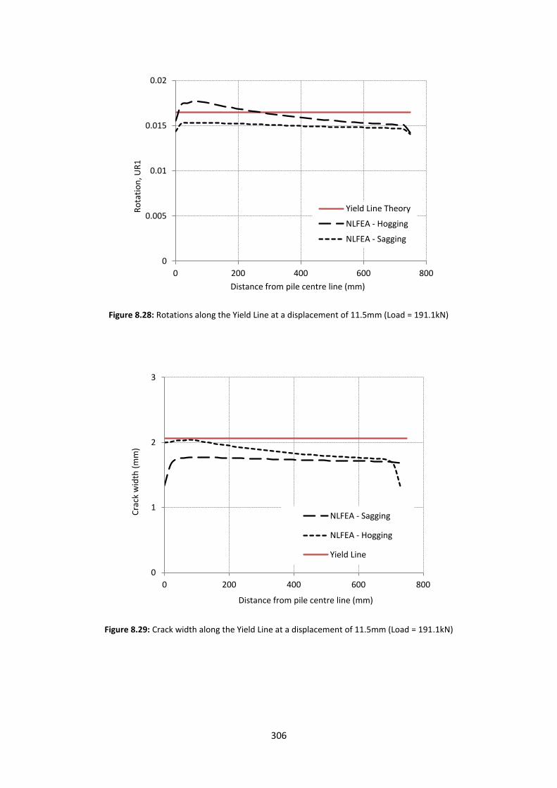
306
Figure 8.28: Rotations along the Yield Line at a displacement of 11.5mm (Load = 191.1kN)
Figure 8.29: Crack width along the Yield Line at a displacement of 11.5mm (Load = 191.1kN)
0
0.005
0.01
0.015
0.02
0 200 400 600 800
Ro
tati
on
, UR
1
Distance from pile centre line (mm)
Yield Line Theory
NLFEA - Hogging
NLFEA - Sagging
0
1
2
3
0 200 400 600 800
Cra
ck w
idth
(m
m)
Distance from pile centre line (mm)
NLFEA - Sagging
NLFEA - Hogging
Yield Line
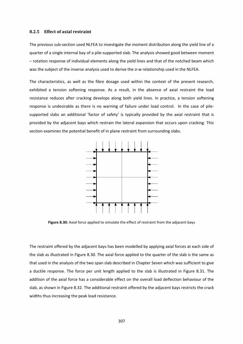
307
8.2.5 Effect of axial restraint
The previous sub-section used NLFEA to investigate the moment distribution along the yield line of a
quarter of a single internal bay of a pile-supported slab. The analysis showed good between moment
– rotation response of individual elements along the yield lines and that of the notched beam which
was the subject of the inverse analysis used to derive the σ-w relationship used in the NLFEA.
The characteristics, as well as the fibre dosage used within the context of the present research,
exhibited a tension softening response. As a result, in the absence of axial restraint the load
resistance reduces after cracking develops along both yield lines. In practice, a tension softening
response is undesirable as there is no warning of failure under load control. In the case of pile-
supported slabs an additional ‘factor of safety’ is typically provided by the axial restraint that is
provided by the adjacent bays which restrain the lateral expansion that occurs upon cracking. This
section examines the potential benefit of in plane restraint from surrounding slabs.
Figure 8.30: Axial force applied to simulate the effect of restraint from the adjacent bays
The restraint offered by the adjacent bays has been modelled by applying axial forces at each side of
the slab as illustrated in Figure 8.30. The axial force applied to the quarter of the slab is the same as
that used in the analysis of the two span slab described in Chapter Seven which was sufficient to give
a ductile response. The force per unit length applied to the slab is illustrated in Figure 8.31. The
addition of the axial force has a considerable effect on the overall load deflection behaviour of the
slab, as shown in Figure 8.32. The additional restraint offered by the adjacent bays restricts the crack
widths thus increasing the peak load resistance.
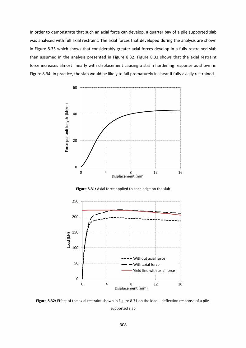
308
In order to demonstrate that such an axial force can develop, a quarter bay of a pile supported slab
was analysed with full axial restraint. The axial forces that developed during the analysis are shown
in Figure 8.33 which shows that considerably greater axial forces develop in a fully restrained slab
than assumed in the analysis presented in Figure 8.32. Figure 8.33 shows that the axial restraint
force increases almost linearly with displacement causing a strain hardening response as shown in
Figure 8.34. In practice, the slab would be likely to fail prematurely in shear if fully axially restrained.
Figure 8.31: Axial force applied to each edge on the slab
Figure 8.32: Effect of the axial restraint shown in Figure 8.31 on the load – deflection response of a pile-
supported slab
0
20
40
60
0 4 8 12 16
Forc
e p
er u
nit
len
gth
(kN
/m)
Displacement (mm)
0
50
100
150
200
250
0 4 8 12 16
Load
(kN
)
Displacement (mm)
Without axial force
With axial force
Yield line with axial force
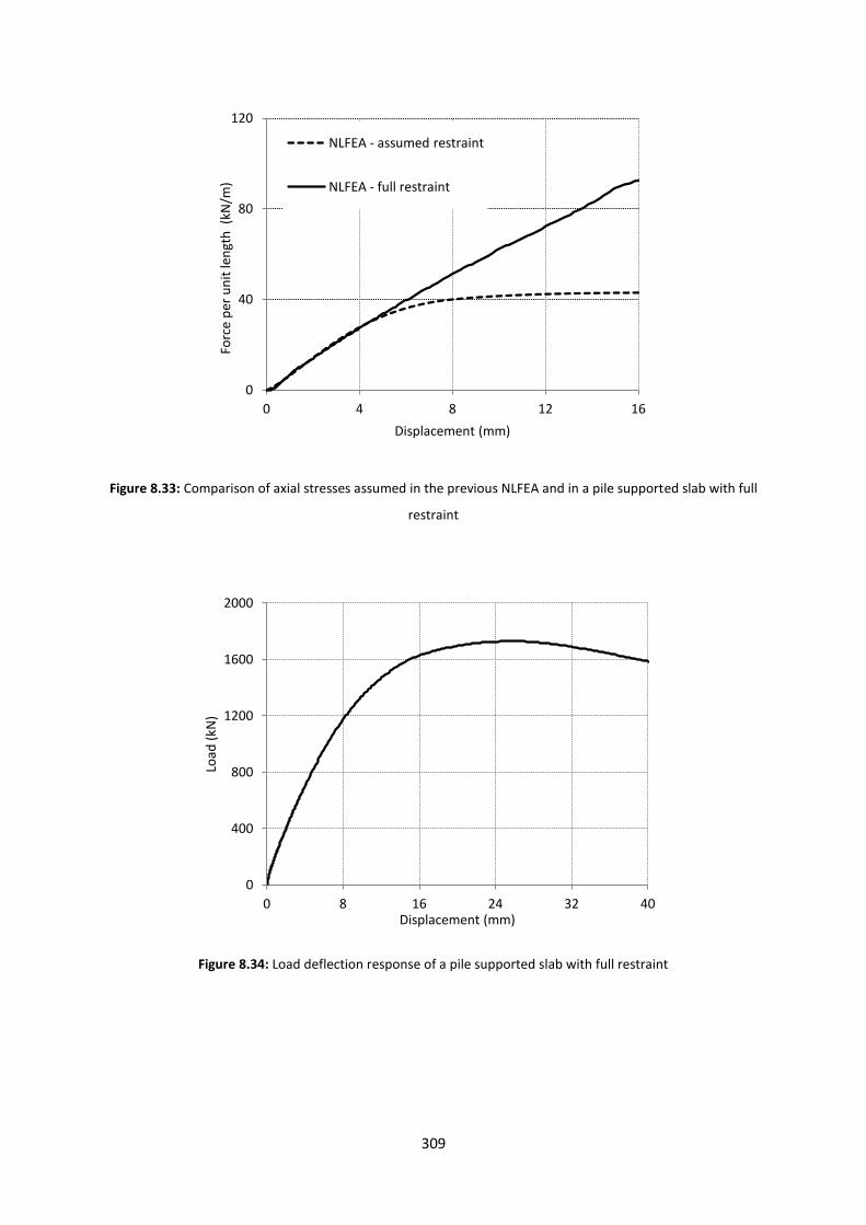
309
Figure 8.33: Comparison of axial stresses assumed in the previous NLFEA and in a pile supported slab with full
restraint
Figure 8.34: Load deflection response of a pile supported slab with full restraint
0
40
80
120
0 4 8 12 16
Forc
e p
er u
nit
len
gth
(kN
/m)
Displacement (mm)
NLFEA - assumed restraint
NLFEA - full restraint
0
400
800
1200
1600
2000
0 8 16 24 32 40
Load
(kN
)
Displacement (mm)
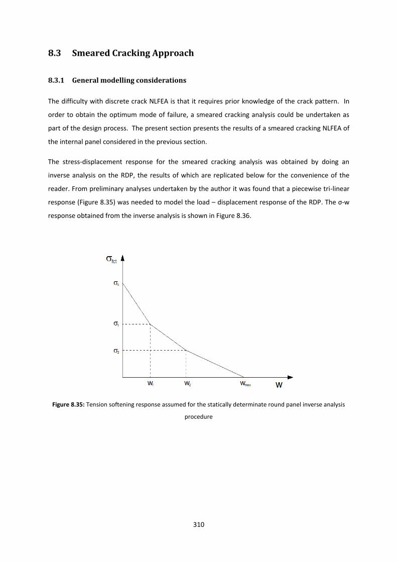
310
8.3 Smeared Cracking Approach
8.3.1 General modelling considerations
The difficulty with discrete crack NLFEA is that it requires prior knowledge of the crack pattern. In
order to obtain the optimum mode of failure, a smeared cracking analysis could be undertaken as
part of the design process. The present section presents the results of a smeared cracking NLFEA of
the internal panel considered in the previous section.
The stress-displacement response for the smeared cracking analysis was obtained by doing an
inverse analysis on the RDP, the results of which are replicated below for the convenience of the
reader. From preliminary analyses undertaken by the author it was found that a piecewise tri-linear
response (Figure 8.35) was needed to model the load – displacement response of the RDP. The σ-w
response obtained from the inverse analysis is shown in Figure 8.36.
Figure 8.35: Tension softening response assumed for the statically determinate round panel inverse analysis
procedure
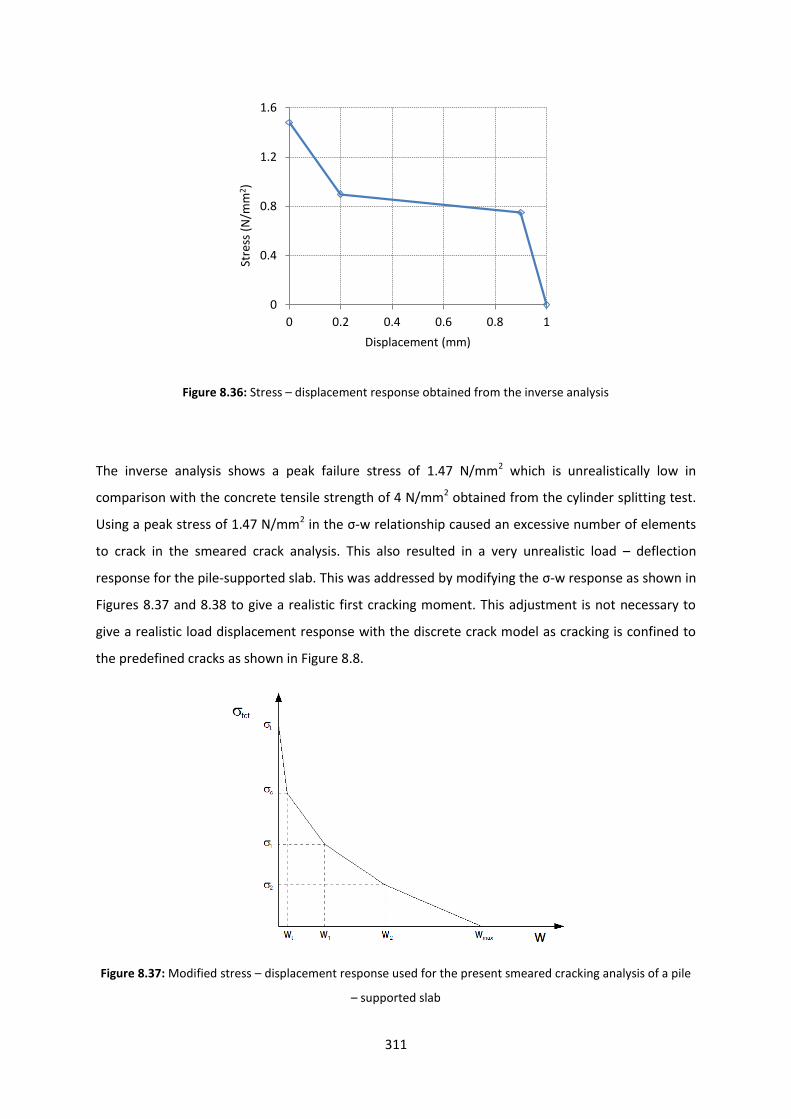
311
Figure 8.36: Stress – displacement response obtained from the inverse analysis
The inverse analysis shows a peak failure stress of 1.47 N/mm2 which is unrealistically low in
comparison with the concrete tensile strength of 4 N/mm2 obtained from the cylinder splitting test.
Using a peak stress of 1.47 N/mm2 in the σ-w relationship caused an excessive number of elements
to crack in the smeared crack analysis. This also resulted in a very unrealistic load – deflection
response for the pile-supported slab. This was addressed by modifying the σ-w response as shown in
Figures 8.37 and 8.38 to give a realistic first cracking moment. This adjustment is not necessary to
give a realistic load displacement response with the discrete crack model as cracking is confined to
the predefined cracks as shown in Figure 8.8.
Figure 8.37: Modified stress – displacement response used for the present smeared cracking analysis of a pile
– supported slab
0
0.4
0.8
1.2
1.6
0 0.2 0.4 0.6 0.8 1
Stre
ss (
N/m
m2 )
Displacement (mm)
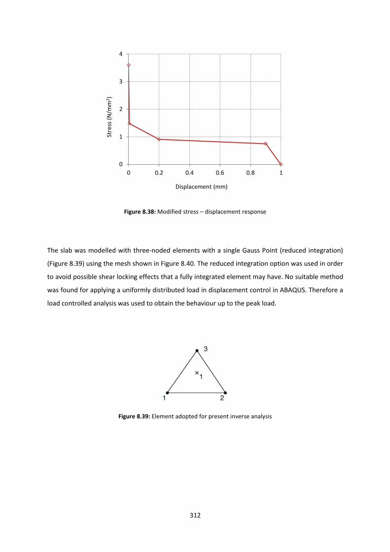
312
Figure 8.38: Modified stress – displacement response
The slab was modelled with three-noded elements with a single Gauss Point (reduced integration)
(Figure 8.39) using the mesh shown in Figure 8.40. The reduced integration option was used in order
to avoid possible shear locking effects that a fully integrated element may have. No suitable method
was found for applying a uniformly distributed load in displacement control in ABAQUS. Therefore a
load controlled analysis was used to obtain the behaviour up to the peak load.
Figure 8.39: Element adopted for present inverse analysis
0
1
2
3
4
0 0.2 0.4 0.6 0.8 1
Stre
ss (
N/m
m2 )
Displacement (mm)
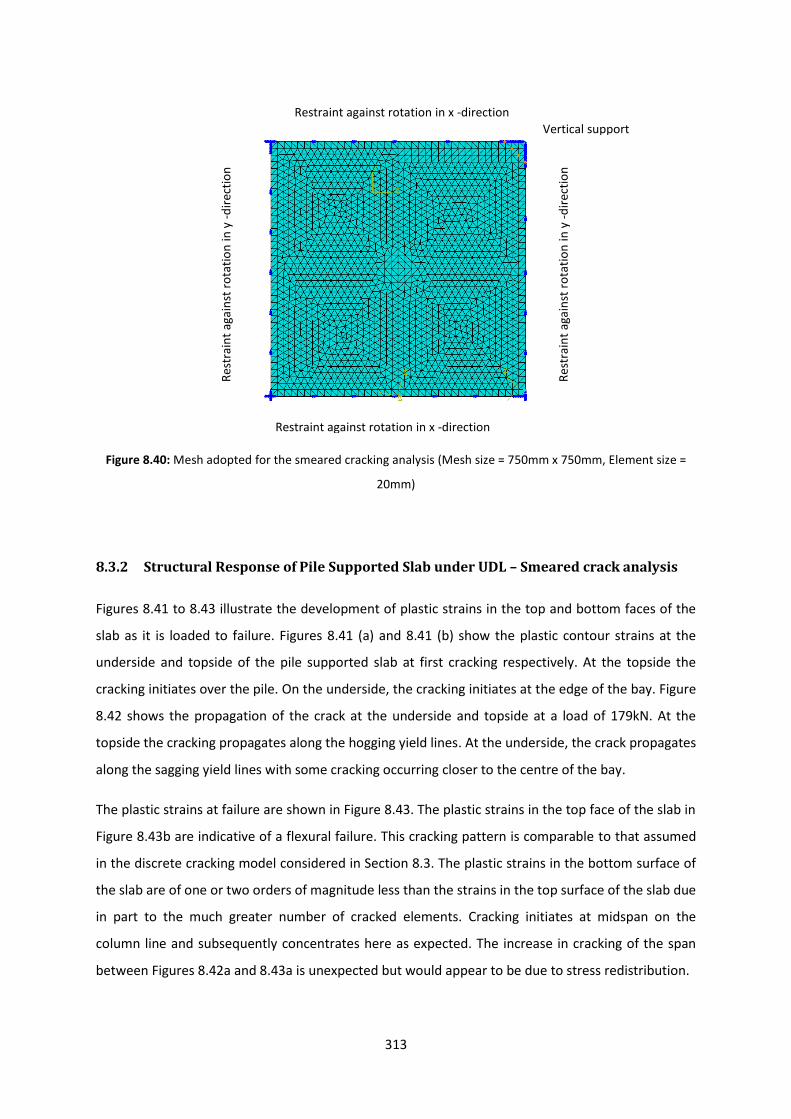
313
Figure 8.40: Mesh adopted for the smeared cracking analysis (Mesh size = 750mm x 750mm, Element size =
20mm)
8.3.2 Structural Response of Pile Supported Slab under UDL – Smeared crack analysis
Figures 8.41 to 8.43 illustrate the development of plastic strains in the top and bottom faces of the
slab as it is loaded to failure. Figures 8.41 (a) and 8.41 (b) show the plastic contour strains at the
underside and topside of the pile supported slab at first cracking respectively. At the topside the
cracking initiates over the pile. On the underside, the cracking initiates at the edge of the bay. Figure
8.42 shows the propagation of the crack at the underside and topside at a load of 179kN. At the
topside the cracking propagates along the hogging yield lines. At the underside, the crack propagates
along the sagging yield lines with some cracking occurring closer to the centre of the bay.
The plastic strains at failure are shown in Figure 8.43. The plastic strains in the top face of the slab in
Figure 8.43b are indicative of a flexural failure. This cracking pattern is comparable to that assumed
in the discrete cracking model considered in Section 8.3. The plastic strains in the bottom surface of
the slab are of one or two orders of magnitude less than the strains in the top surface of the slab due
in part to the much greater number of cracked elements. Cracking initiates at midspan on the
column line and subsequently concentrates here as expected. The increase in cracking of the span
between Figures 8.42a and 8.43a is unexpected but would appear to be due to stress redistribution.
Restraint against rotation in x -direction
Restraint against rotation in x -direction
Res
trai
nt
agai
nst
ro
tati
on
in y
-d
irec
tio
n
Res
trai
nt
agai
nst
ro
tati
on
in y
-d
irec
tio
n
Vertical support
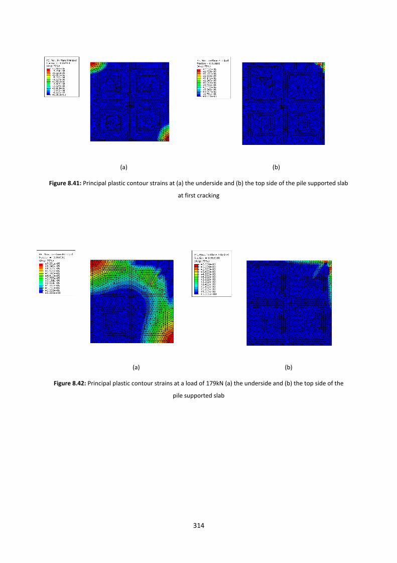
314
(a) (b)
Figure 8.41: Principal plastic contour strains at (a) the underside and (b) the top side of the pile supported slab
at first cracking
(a) (b)
Figure 8.42: Principal plastic contour strains at a load of 179kN (a) the underside and (b) the top side of the
pile supported slab
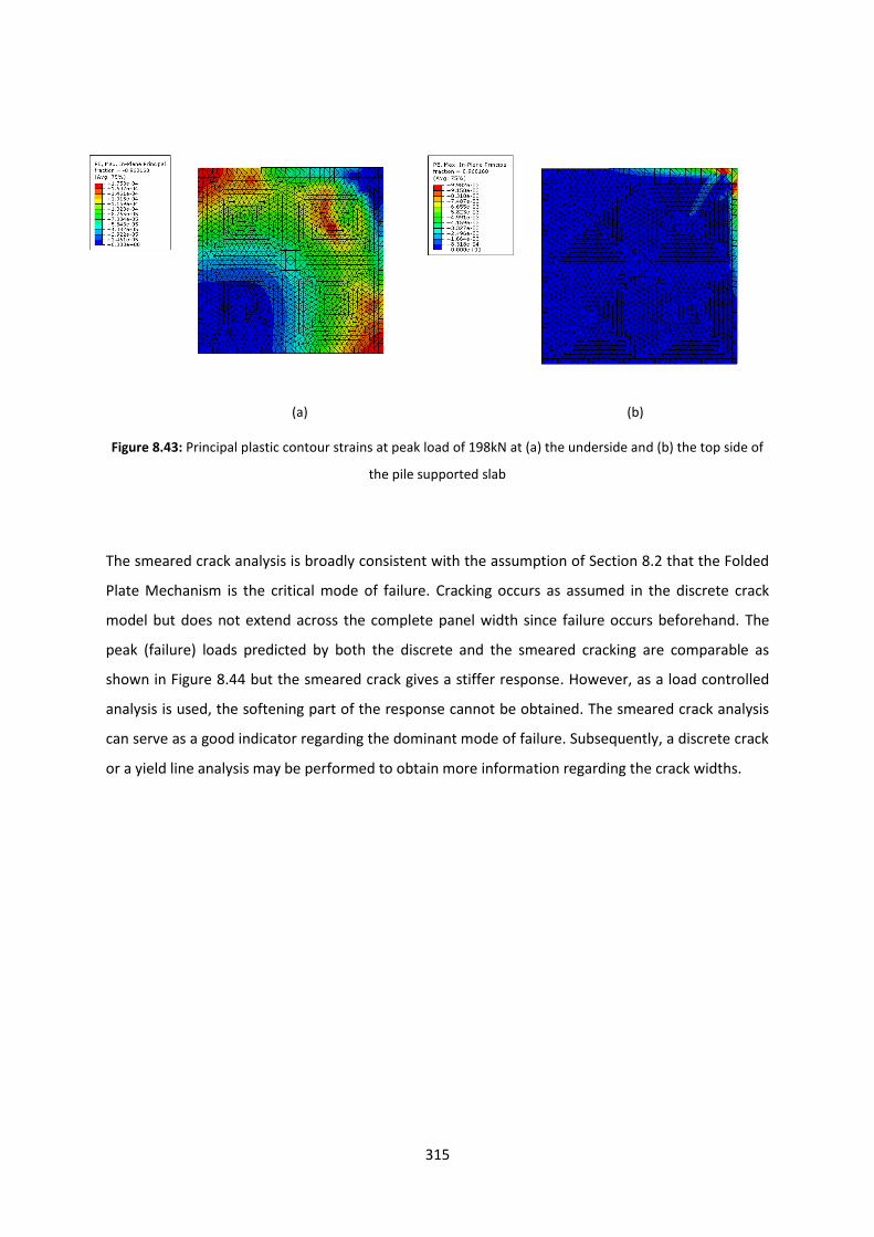
315
(a) (b)
Figure 8.43: Principal plastic contour strains at peak load of 198kN at (a) the underside and (b) the top side of
the pile supported slab
The smeared crack analysis is broadly consistent with the assumption of Section 8.2 that the Folded
Plate Mechanism is the critical mode of failure. Cracking occurs as assumed in the discrete crack
model but does not extend across the complete panel width since failure occurs beforehand. The
peak (failure) loads predicted by both the discrete and the smeared cracking are comparable as
shown in Figure 8.44 but the smeared crack gives a stiffer response. However, as a load controlled
analysis is used, the softening part of the response cannot be obtained. The smeared crack analysis
can serve as a good indicator regarding the dominant mode of failure. Subsequently, a discrete crack
or a yield line analysis may be performed to obtain more information regarding the crack widths.
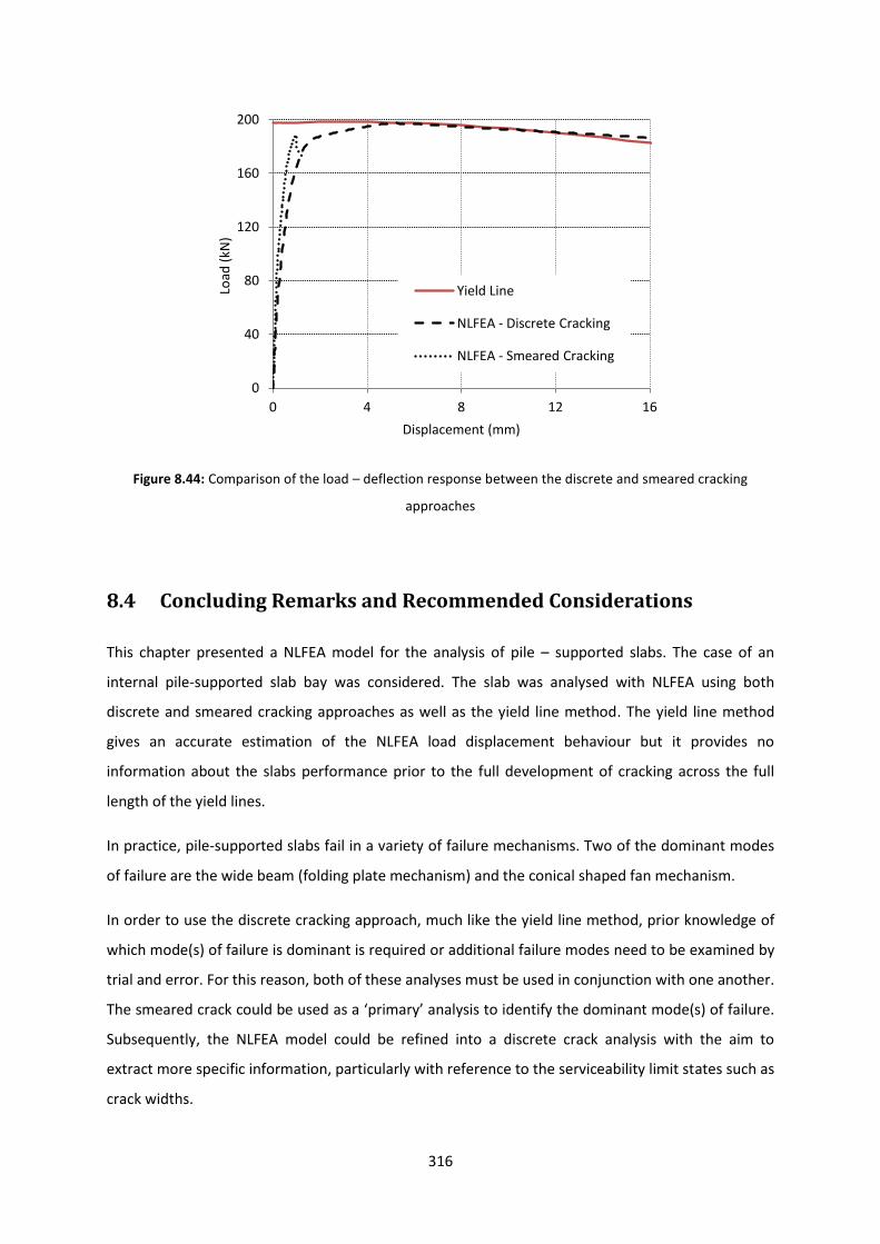
316
Figure 8.44: Comparison of the load – deflection response between the discrete and smeared cracking
approaches
8.4 Concluding Remarks and Recommended Considerations
This chapter presented a NLFEA model for the analysis of pile – supported slabs. The case of an
internal pile-supported slab bay was considered. The slab was analysed with NLFEA using both
discrete and smeared cracking approaches as well as the yield line method. The yield line method
gives an accurate estimation of the NLFEA load displacement behaviour but it provides no
information about the slabs performance prior to the full development of cracking across the full
length of the yield lines.
In practice, pile-supported slabs fail in a variety of failure mechanisms. Two of the dominant modes
of failure are the wide beam (folding plate mechanism) and the conical shaped fan mechanism.
In order to use the discrete cracking approach, much like the yield line method, prior knowledge of
which mode(s) of failure is dominant is required or additional failure modes need to be examined by
trial and error. For this reason, both of these analyses must be used in conjunction with one another.
The smeared crack could be used as a ‘primary’ analysis to identify the dominant mode(s) of failure.
Subsequently, the NLFEA model could be refined into a discrete crack analysis with the aim to
extract more specific information, particularly with reference to the serviceability limit states such as
crack widths.
0
40
80
120
160
200
0 4 8 12 16
Load
(kN
)
Displacement (mm)
Yield Line
NLFEA - Discrete Cracking
NLFEA - Smeared Cracking
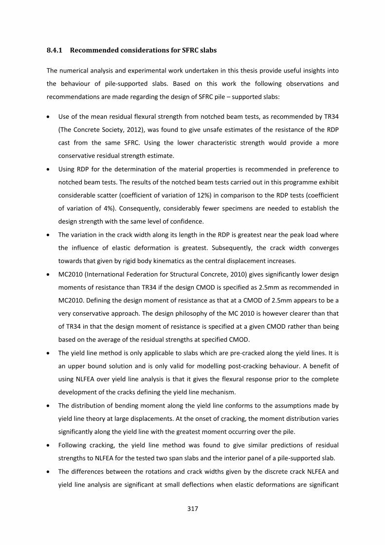
317
8.4.1 Recommended considerations for SFRC slabs
The numerical analysis and experimental work undertaken in this thesis provide useful insights into
the behaviour of pile-supported slabs. Based on this work the following observations and
recommendations are made regarding the design of SFRC pile – supported slabs:
Use of the mean residual flexural strength from notched beam tests, as recommended by TR34
(The Concrete Society, 2012), was found to give unsafe estimates of the resistance of the RDP
cast from the same SFRC. Using the lower characteristic strength would provide a more
conservative residual strength estimate.
Using RDP for the determination of the material properties is recommended in preference to
notched beam tests. The results of the notched beam tests carried out in this programme exhibit
considerable scatter (coefficient of variation of 12%) in comparison to the RDP tests (coefficient
of variation of 4%). Consequently, considerably fewer specimens are needed to establish the
design strength with the same level of confidence.
The variation in the crack width along its length in the RDP is greatest near the peak load where
the influence of elastic deformation is greatest. Subsequently, the crack width converges
towards that given by rigid body kinematics as the central displacement increases.
MC2010 (International Federation for Structural Concrete, 2010) gives significantly lower design
moments of resistance than TR34 if the design CMOD is specified as 2.5mm as recommended in
MC2010. Defining the design moment of resistance as that at a CMOD of 2.5mm appears to be a
very conservative approach. The design philosophy of the MC 2010 is however clearer than that
of TR34 in that the design moment of resistance is specified at a given CMOD rather than being
based on the average of the residual strengths at specified CMOD.
The yield line method is only applicable to slabs which are pre-cracked along the yield lines. It is
an upper bound solution and is only valid for modelling post-cracking behaviour. A benefit of
using NLFEA over yield line analysis is that it gives the flexural response prior to the complete
development of the cracks defining the yield line mechanism.
The distribution of bending moment along the yield line conforms to the assumptions made by
yield line theory at large displacements. At the onset of cracking, the moment distribution varies
significantly along the yield line with the greatest moment occurring over the pile.
Following cracking, the yield line method was found to give similar predictions of residual
strengths to NLFEA for the tested two span slabs and the interior panel of a pile-supported slab.
The differences between the rotations and crack widths given by the discrete crack NLFEA and
yield line analysis are significant at small deflections when elastic deformations are significant
318
but reduce with increasing deflection as expected due to the reduced significance of elastic
deformations which are neglected in yield line analysis.
The effect of the axial restraint can be accounted for with a good level of accuracy by adding
0.5Nh to the yield line moment of resistance.
The smeared cracking NLFEA predictions are comparable with those of the discrete crack
formulation when displacement control can be used. On the other hand, the discrete crack
analysis, which requires prior knowledge of the crack pattern, allows for a more in-depth
analysis of the structure allowing for the calculation of plastic strains and crack widths. The
smeared cracking approach can be used for the identification of the critical failure mechanism to
be used in discrete crack model.
The punching shear tests showed the twisted Helix fibres to work best of the tested fibres as
failure was due to fibre pullout rather than rupture. The hooked end fibres performed less well
as the fibres fractured at failure rather than pulling out as desired. Fibre rupture can be avoided
by either lowering the concrete strength or alternatively using a higher strength fibre. The tests
showed that punching shear resistance can be significantly increased by fibres and that TR34
(The Concrete Society, 2012) underestimates their contribution to shear resistance. This relates
to the discussion in Chapter 7.
319
Chapter Nine
Conclusions
9.1 Recapitulation
The use of SFRC in the design of pile supported slabs can bring a number of benefits. The primary
aim of this research project was to investigate the behaviour and design of pile supported slabs with
particular emphasis on the post-cracking response.
Firstly, a comprehensive literature review was performed in order to gain an insight into the issues
commonly found in SFRC slabs. The shortcomings of current design provisions and design methods
were critically reviewed. This information was subsequently used to formulate a research plan which
included both experimental and numerical work.
An experimental programme was undertaken to a) compare the material properties obtained from
the notched beam and the round determinate plate tests and b) determine a relationship between
the residual strengths given by each method. An innovative test setup was designed to measure
crack widths during round plate tests. This allowed a direct relationship to be determined between
the crack width and the central displacement of the panel. Both monotonic and cyclic loading
conditions were investigated. Three two span slabs were tested to simulate the Folded Plate
mechanism that occurs in SFRC pile-supported slabs. The effect of axial restraint was considered in
one of these tests.
The third stage involved non-linear finite element modelling. This involved selection of appropriate
material models to capture the behaviour of SFRC. A series of sensitivity studies were undertaken to
obtain numerical parameters for input into the NLFEA. The inverse analysis procedure was used to
obtain a stress – crack width response for the numerical modelling. The numerical modelling allowed
for a more in-depth investigation into the failure of round determinate plates and two span slabs
than given by yield line analysis.
The numerical model was then extended to model a bay of a pile-supported slab under a uniformly
distributed load. The main conclusions of the research are summarised in the next sections.

320
9.2 Conclusions from literature survey
The main conclusions are as follows:
There are a number of different test methods used to determine the strength of SFRC after
cracking. However, there is no agreement regarding which method is the best. As a result
different fibre suppliers claim different properties resulting in confusion amongst designers.
At the dosages presently used in industry (between 35 – 45 kg/m3) notched beam tests exhibit a
tension softening response. However, due to load re-distribution as well as axial restraint there
is some evidence from large scale tests that slabs reinforced with such dosages of fibres show a
tension hardening response.
It is claimed by some manufacturers that statically indeterminate panel tests can be more
representative of the actual behaviour of SFRC pile-supported slabs than notched beam tests.
However, it is difficult to extract the material properties of SFRC from indeterminate plate tests
as the stress distribution is not known due to the indeterminate boundary conditions.
9.3 Shortcomings of current design guidelines
The following conclusions were drawn from the literature review of current design provisions for
SFRC pile-supported slabs.
Elastic methods for the design of SFRC pile-supported slabs are inefficient as the addition of steel
fibres in the dosages commonly used does not increase the peak load resistance. The fibres
mainly come into effect after the peak flexural load by bridging and arresting crack growth.
The yield line method is considered the most suitable method for designing pile supported slabs.
However, there is a lack of agreement on the choice of the design bending moment of resistance
as it reduces with increasing crack width. Membrane effects in slabs are commonly ignored in the
yield line method although they can be accounted for.
The yield line method assumes that all the curvature of the slab is concentrated as rotations in
the yield line with the regions in between behaving as rigid bodies. In reality, this is a close
approximation to the behaviour of SFRC slabs at large deflections. However, this does not give a
true depiction of the behaviour prior to cracking and at small crack widths when elastic
deformations are significant.
The design codes do not include any guidelines for the calculation of the crack widths in SFRC
pile-supported slabs without traditional steel reinforcement.
321
9.4 Conclusions from experimental work
The conclusions from the experimental works undertaken can be summarised as follows:
The fibre dispersion and orientation had a significant effect on the load deflection response of
the notched beam tests.
The RDPs tested in the present experimental programme exhibited different crack patterns but
the variation in angles between the cracks did not affect significantly the load deflection response
as found by Bernard et al. (2008). However, the crack – displacement response followed by each
crack is dependent on its position.
The crack widths observed in the RDP varied considerably along the length of the cracks, near the
peak load, with the greatest width occurring under the loading plate and reducing with increasing
distance from the centre of the plate. The crack width becomes almost uniform along its length at
larger displacements when the elastic deformation becomes negligible in comparison with the
total displacement. The crack width through the slab thickness is non-linear during the early
loading stages. However, it becomes linear with increasing displacement suggesting that the
individual segments behave like rigid bodies at large displacements as assumed in the yield line
method.
Cyclic loading can impair significantly the performance of a cracked slab. The cyclic load test
undertaken showed that during unloading the cracks do not return to their original positions. The
slip of the fibres prevents complete crack closing.
A significant difference between the RDP and the notched beam test is that the position of the
crack is fixed in the beam test as it can only form at the notch. This is not the case for the RDP,
where the cracks form at the positions where the tangential bending moment first equals the
cracking moment.
The notched beam tests exhibit considerably more scatter (coefficient of variation of 12%) in
comparison to the RDP (coefficient of variation of 4%).
The increase in shear resistance due to the addition of the steel fibres was 0.5MPa and 0.7MPa in
the specimens reinforced with one hoop (Type I) and reinforced with two hoops (Type II)
respectively. Technical Report 34 underestimated the contribution of the steel fibres to the shear
resistance especially for Type II tests.

322
9.5 Conclusions from present NLFEA
The moment – rotation response extracted from the notched beam tests did not simulate the
RDP responses accurately. The use of the mean residual flexural strengths from the notched
beam tests was found to give unsafe predictions of the strengths of the RDP.
The average residual strengths obtained from the notched beam tests are considerably greater
than the ones obtained for the RDP particularly for CMOD larger than 1mm. This can be
attributed to the fact that the crack position in the beam was predetermined due to the notch
whereas the slab was allowed to fail at its weakest position. The mould side effect which causes
fibres to become aligned parallel to the mould faces may have also contributed to the greater
strength of the notched beams.
The design moments of resistance given by Technical Report 34 (The Concrete Society, 2012) and
Model Code 2010 (International Federation for Structural Concrete, 2010) (with material factor of
safety equal to one) are relatively conservative compared with the peak moments of resistance
back calculated from the results of the RDP using yield line analysis. MC2010 is more conservative
than Technical Report 34 if the design moment of resistance is calculated at a CMOD of 2.5mm as
recommended.
The yield line method, non linear beam analysis and the present NLFEA show good agreement in
the prediction of the response of the two span slab. The discrete cracking approach gave a more
accurate prediction of the load – deflection response than the smeared cracking approach.
However the main drawback of the discrete crack method is that the location of the cracks has to
be predetermined. The crack patterns observed were similar for both the discrete and the
smeared cracking approaches. However, the number of elements that cracked was greater in the
smeared crack analysis for comparable element sizes. Realistic crack width predictions can only
be extracted from a discrete crack analysis.
NLFEA provides a complete load deflection response unlike the yield line analysis which only
applies to a fully cracked slab.
Axial restraint can significantly increase the flexural resistance of SFRC slabs. The studies
undertaken on the two – span slab and the internal bay of a pile-supported slab showed that the
axial restraint offered by the adjacent panels can produce a strain hardening response despite
the fact that the material response is a softening one.
The moment varies along the yield lines in SFRC slabs. This is true particularly during and shortly
after the onset of cracking. As the crack develops, the individual segments behave more like rigid

323
bodies. As a result the rotation becomes concentrated in the cracks and the moment becomes
uniform.
9.5 Recommended Considerations
The recommendations stemming from this research are as follows:
Using the mean residual flexural strength obtained from the notched beam provides an unsafe
estimate of the structural behaviour of the RDP.
Using the RDP for the determination of the material properties is recommended rather than the
notched beam tests due to the smaller scatter.
MC2010 gives significantly lower design moments of resistance than TR34 if the design CMOD is
specified as 2.5mm in MC2010 as recommended. Using the MC2010 gives a clearer design
guideline as the design moment of resistance is calculated at a specified crack width rather than
being calculated with the average of the residual flexural strengths at specified CMOD.
The yield line method predicted the NLFEA results for the two span slab and the pile - supported
slab quarter bay accurately after crack initiation.
The yield line method does not predict the response up to the first crack. The yield line method
is an upper bound solution and is only valid for the post-cracking behaviour of the RDP.
The variation in the crack width along its length in the RDP is greatest near the peak load where
the influence of elastic deformation is greatest. Subsequently, the crack width converges
towards that given by rigid body kinematics as the central displacement increases.
The effect of the axial restraint can be accounted for with a good level of accuracy by adding
0.5Nh to the yield line moment. The yield line approach predicts the experimental results with a
significant level of accuracy at large displacements as the slab behaves more like a rigid body.
The smeared cracking approach predictions are comparable with those of the discrete crack. On
the other hand, the discrete crack analysis, which requires prior knowledge of the crack pattern,
allows for a more in-depth analysis of the structure allowing for the calculation of plastic strains
and crack widths.
The punching shear tests showed the Helix fibres to work best of the tested fibres as failure was
due to fibre pullout rather than rupture. The hooked end fibres performed less well as the fibres
fractured at failure rather than pulling out as desired. Fibre rupture can be avoided by either
lowering the concrete strength or alternatively using a higher strength fibre.

324
9.6 Recommendations for future research
This thesis provided a contribution in the behaviour and design of pile supported slabs. There are a
number of topics which have not yet been addressed:
Using the methodology from the present study, a more comprehensive study into the effect of
cyclic loading in pile supported slabs with particular reference to the crack widths. This study
could also be extended to take account of dynamic loads.
Development of design guidelines for the estimation of the critical crack width in SFRC pile-
supported slabs.
The effect of drying shrinkage and early age thermal stresses on the stresses and strains that
develop in pile-supported slabs.
The methodology of the present study could also be used to investigate the design and behaviour
of SFRC suspended slabs for cases where some or all of the reinforcement has been substituted
with steel fibres.
The effect of axial restraint requires further consideration as its presence is necessary for a strain
hardening response at the fibre dosages commonly used in pile-supported slabs.
Additional investigations to determine the significance of the distribution of the steel fibres in the
structural behaviour of pile supported slabs.
The potential degradation of the axial restraint present in pile supported slabs.
325
Bibliography
Abbas, A. A. (2002). Analysis and Design of Industrial Ground-Floor Slabs using the Finite Element
Method PhD Thesis. Imperial College, London.
ACI Committee. (1999). Design Considerations for Steel Fiber Reinforced Concrete. American
Concrete Institute, Detroit.
Alexander, S., & Simmonds, S. (1992). Punching shear tests of concrete - Column joints containing
fibre-reinforcement. ACI Structural Journal , 89 (4), 425-432.
American Society for Testing and Materials . (2004). ASTM C1399, Test Method for obtaining average
residual strength of fiber-reinforced concrete. American Society for Testing and Materials, USA, 2004.
American Society for Testing and Materials. (2005). ASTM C 1609, Standard test method for flexural
performance of fiber-reinforced concrete (using beam with third-point loading). American Society for
Testing and Materials, USA.
American Society of Civil Engineers. (1985). Finite Element Analysis of Reinforced Concrete
Structures: Proceedings of the Seminar sponsored by the Japan Society for the Promotion of Science
and the U.S. National Science Foundation. American Society of Civil Engineers, New York.
ArcelorMittal Sheffield Ltd. (2009). ArcelorMittal Steel-Fibre-Reinforced Concrete. ArchelorMittal
Sheffield Ltd, Sheffield.
Arnaouti, C. (1972). Yield criteria for reinforced concrete slabs PhD Thesis. University of Aston,
Birmingham.
ASTM. (2004). C1550 Standard Test Method for Flexural Toughness of Fiber Reinforced Concrete
(using centrally loaded round panel). West Conshocken, Pennsylvania, USA: ASTM International.
Austin, S., Jones, P., Armelin, H., & Robins, P. (2006). Prediction of steel fibre reinforced concrete
under flexure from an inferred fibre pull-out response. Materials and Structures , 601-610.
Balakrishnan, S., & Murray, D. W. (1998). Concrete Constitutive Model for NLFE Analysis of
Structures. Journal of Structural Engineering , 114 (7), 1449-1466.
Banthia, N., & Trottier, J. F. (1994). Concrete reinforced with deformed steel fibres part 1: bond slip
mechanisms. ACI Material Journal , 91 (5), 435 - 446.
326
Banthia, N., Gupta, P., & Yan, C. (1999). Impact Resistance of Fibre Reinforced Wet-Mix Shotcrete-
Part 2: Plate Tests. Materials and Structures , 32, 643-650.
Barros, J. A., & Figueiras, J. A. (1998). Experimental behaviour of fibre concrete slabs on soil.
Mechanics of Cohesive Frictional Materials , 3, 277-290.
Barros, J. A., & Figueiras, J. A. (1999). Flexural Behavior of SFRC: Testing and Modelling. Journal of
Materials in Civil Engineering , 11 (4), 331-339.
Barros, J. A., & Sena Cruz, J. (2001). Fracture Energy of Steel Fibre Reinforced Concrete. Mechanics of
composite materials and structures , 8 (1), 29-45.
Barros, J. A., Cunha, V. M., Ribeiro, A. F., & Antunes, J. A. (2005). Post-cracking behaviour of steel-
fibre reinforced concrete. Materials and Structures , 38, 47-56.
Barros, J., & Antunes, J. Experimental Characterization of the flexural behaviour of steel fibre
reinforced concrete according to RILEM TC 162-TDF recommendations.
Barros, J., & Figueiras, J. (2001). Model for the analysis of steel fibre reinforced concrete slabs on
grade. Computers and Structures , 79, 97-106.
Barros, J., Ventura Gouveia, A., Antunes, J., & Azevedo, A. Design Methods for Streel Fiber Reinforced
Concrete Industrial Floors.
Bazant, Z. P. (1983). Crack band theory for fracture of concrete. Materials and Structures , 16, 155-
177.
Bazant, Z. P., & Oh, B. H. (1983). Crack band theory for fracture of concrete. Materials and Structures
, 16, 155-177.
Belletti, B., Bernardi, P., Meda, A., & Plizzari, G. (2006). A NLFM Method for the Prediction of Slabs on
Grade Behaviour.
Belletti, B., Cerioni, R., & Plizzari, G. (2008). Design Aspects on Steel Fiber-Reinforced Concrete
Pavements. Journal of Materials in Civil Engineering , 20 (9), 599-607.
Bernard, E. S. (2000). Behaviour of round steel fibre reinforced concrete panels under point loads.
Materials and Structures , 33, 181-188.
Bernard, E. S. (2002). Correlations in the behaviour of fibre reinforced shotcrete beam and panel
specimens. Materials and Strcutures , 35, 156-164.
327
Bernard, E. S. (2005). The Role of Friction in Post-Crack Energy Absorption of Fiber Reinforced
Concrete in the Round Panel Test. Journal of ASTM International , 2 (1), 1-12.
Bernard, E. S., & Pircher, M. (2000). Engineering Report No. CE10 - Influence of Geometry on
Performance of Round Determinate Panels made with Fibre Reinforced Concrete. School of Civic and
Environment, University of Western Sidney, Kingswood, Australia.
Bernard, E. S., & Pircher, M. (2000). The Influence of Thickness on Performance of Fiber-Reinforced
Concrete in a Round Determinate Panel Test. Cement, Concrete and Aggregates , 23 (1), 27-33.
Bernard, E. S., & Xu, G. G. (2008). The Effect of Radial Crack Locations on Load Resistance in C1550
Panel Tests. Journal of ASTM International , 5 (10), 1-14.
Bernard, E. S., Tran, V. N., & Beasley, A. J. (2001). Application of Yield Line Theory to Round
Determinate Panels. Engineering Developments In Shotcrete (International Conference) April 2001 ,
245-254.
Bhatt, P., MacGinley, J., & Choo, B. S. (2006). Reinforced Concrete: Design Theory and Examples.
Taylor & Francis, , Abingdon.
Bishop, J. W. (2001). The Early Age Behaviour of Concrete Industrial Ground Floor Slabs PhD Thesis.
Loughborough University.
Braestrup, M. W. (1970). Yield-line Theory and Limit Analysis of Plates and Slabs. Concrete Research ,
22 (71), 99-106.
British Standards Institution. (2009). BS EN 12390-5: 2009 Testing hardened concrete Part 5: Flexural
strength of test specimens. British Standards Institution, London.
British Standards Institution. (2005). BS EN 14651:2005 - Test Method for Metallic Fibre Concrete -
Measuring the Flexural Tensile Strength (Limit of Proportionality (LOP), Residual). British Standards
Institution, London.
British Standards Institution. (2007). BS EN 14845-1:2007 - Test Methods for Fibres in Concrete - Part
1: Reference Concretes. British Standards Institution, London.
British Standards Institution. (2006). BS EN 14845-2:2006 - Test Methods for Fibres in Concrete - Part
2: Effect on Concrete. British Standards Institution, London.
British Standards Institution. (2006). BS EN: 14889-1:2006 : Steel fibres - Definitions, specifications
and conformity. British Standards Institution, London.

328
British Standards Institution. (2004). BS EN: 1992-1-1:2004: General Rules and Rules for Buildings.
British Standards Institution, London.
Casanova, P., & Rossi, P. (1997). Analysis and design of steel fibre reinforced concrete beams. ACI
Structural Journal , 94 (5), 595-602.
Cement and Concrete Association. (1965). Recent Developments in Yield-Line Theory - MCR Special
Publication. Cement and Concrete Association, London.
Chandler, J. W. (1982). Design of floors on ground. Cement and Concrete Association, Slough.
Chanvillard, G., & Roque, O. (1999). Behavior of Fibre Reinforced Concrete Cracked Section Under
Sustained Load. Third International Workshop on High Performance Fiber Reinforced Cement
Composites (HPFRCC3), (pp. 239-250). Mainz, Germany.
Chen, S. (2004). Strength of steel fibre reinforced concrete ground slabs. Structures & Buildings , 157
(SB2), 157-163.
Clarke, L. J. (1992). Large Area Pours for Suspended Concrete Slabs. British Cement Association,
Crowthorne.
Concrete Society. (1992). Large Area Pours for Suspended Concrete Slabs. British Cement
Association, Crowthorne.
Criswell, S. (1974). Static and dynamic response of reinforced concrete slab-column connections.
Publication SP-42, ACI , 721-746.
Daniel, I. M., & Ishai, O. (2006). Engineering Mechanics of Composite Materials (Second Edition ed.).
Oxford University Press: Oxford.
de Borst, R., Remmers, J. J., Needleman, A., & Abellan, M. A. (2004). Discrete vs smeared crack
models for concrete fracture: bridging the gap. International Journal for Numerical and Analytical
Methods in Geomechanics , 28, 583-607.
De Montaignac, R., Massicote, B., Charon, J. P., & Nour, A. (2012). Design of SFRC structural
elements: post-cracking tensile strength measurement. Materials and Structures , 45, 609-622.
Destree, X. (2005). Concrete Free Suspended Slabs Reinforced with only Steel Fibres: Full Scale
Testing, Results and Conclusions - Design Examples. International RILEM Workshop on High
Performance Fiber Reinforced Cementitious Composites (HPFRCC) in Structural Applications (pp. 287-
294). Honolulu, Hawai: RILEM Publications.

329
Destree, X. (2004). Structural Application of Steel Fibre as only Reinforcing in Free Suspended
Elevanted Slabs: Conditions - Design - Examples. Sixth RILEM Symposium on Fibre-Reinforced
Concretes (FRC) (pp. 1073-1082). Varena, Italy: RILEM Publications.
Destree, X. (2000). Structural Application of Steel Fibre as Principal Reinforcing: Conditions - Design -
Examples. Fifth RILEM symposium on fibre-reinforced concretes (pp. 291-301). Lyon, France: RILEM
Publications.
Dhir, R. K., Newlands, M. D., McCarthy, M. J., & Paine, K. J. (2008). Harnessing Fibres for Concrete
Construction. Proceedings of the International Conference held at the University of Dundee,.
Scotland, UK.
di Prisco, M., Plizzari, G., & Vandewalle, L. (2009). Fibre Reinforced Concrete: New Design
Perspectives. Materials and Structures , 42, 1261-1281.
Ding, Y., & Wolfgang, K. (2000). Compressive stress-strain relationship of steel fibre-reinforced
concrete at early age. Cement and Concrete Research , 30, 1573-1579.
Dupont, D., & Vandewalle, L. (2005). Distribution of steel fibres in rectangular sections. Cement and
Concrete Composites , 27, 391-398.
Dupont, D., & Vandewalle, L. (2002). Recommendations for finite element analysis of FRC. Report of
subtask 3.5, Brite-EuRam Project BRPR-CT98-0813: Test and design methods for steel fibre reinforced
concrete .
Edgington, J. (1973). Steel Fibre Reinforced Concrete PhD Thesis. University of Surrey.
European Federation of Producers and Applicators of specialist products for structures. (1996).
European specification for sprayed concrete. Aldesrhot: EFNARC.
Eyre, J. R., (1994). In-plane stiffness of reinforced concrete slabs under compressive membrane
action. Magazine of Concrete Research, 46, 67-77.
Eyre, J. R., (2006). Membrane action in ground-bearing slabs, Structures and Buildings, 159, 153-163.
Falkner, H., & Gossla, U. (1999). Pile Supported Reinforced or Prestressed SFRC Ground Slabs. Third
International Workshop on High Performance Fiber Reinforced Cement Composites (HPFRCC3, (pp.
595-602). Mainz, Germany.
Ficklen, W. (1914). Patent No. British Patent No. 11754. United Kingdom.
330
FOSROC. (2007). Conplast 430 - Datasheet. FOSROC, Dubai, United Arab Emirates.
Fricks, T. (1992). Cracking in floor slabs. Concrete International , February 1992, 59-62.
Gerhard Vitt, B. (2011). Understanding Steel Fibre Reinforced Concrete: Guidance to comprehending
an extraordinary material. Bekaert, Belgium.
Gohnert, M. (2000). Collapse Load Analysis of Yield-Line Elements. Engineering Structures , 22, 1048-
1054.
Grace Concrete Products. (2008). Strux 90/40 ASTM C1399 vs ASTM C1609. Grace Construction,
Cambridge.
Grzybowski, M., & Shah, S. P. (1989). Model to Predict Cracking in Fibre Reinforced Concrete due to
Restrained Shrinkage. Magazine of Concrete Research , 148, 125-135.
Gu, Q., Xu, H., & Mindess, S. (2009). An improved Test Method and Numerical Analysis for Crack
Opening Resistance of FRC Round Determinate Panels. Wuhan University Journal of Natural Sciences
, 14 (1), 45-52.
Haselwander, B., Jonas, W., & Riech, H. (1995). Material Equations for Steel Fibre Reinforced
Concrete Members. Nuclear Engineering and Design , 156, 235 - 248.
Hedebratt, J., & Silfwerbrand, J. (2004). An Innovative Approach to the Design of Pile Supported
SFRC Slabs. 6th RILEM Symposium on Fibre-Reinforced Concretes (FRC) - BEFIB 2004, (pp. 945-954).
Varenna, Italy.
Hemmy, O. (2002). Recommendations for finte element analysis of FRC. Report of subtask 3.5, Brite-
EuRam Project BRPR-CT98-0813 .
Hillerborg, A. (1980). Analysis of fracture by means of the fictitious crack model, particularly for fibre
reinforced concrete. The International Journal of Cement Composites , 2 (4), 177-184.
Hillerborg, A. (1991). Application of the fictitious crack model to different types of materials.
International Journal of Fracture , 51, 95-102.
Hillerborg, A. (1975). Strip method of design. Cement and Concrete Association, Slough.
Hillerborg, A., Modeer, M., & Petersson, P. E. (1976). Analysis of Crack Formation and Crack Growth
in Concrete by Means of Fracture Mechanics and Finite Elements. Cement and Concrete Research , 6,
773-782.
331
Hulett, T. (2011). Design and construction of pile-supported concrete industrial floors. Concrete , 41-
43.
Illston, J. M., & Domone, P. L. (2004). Construction Materials - Their Nature and Behaviour (Third
ed.). Spon Press, London.
International Federation for Structural Concrete. (2010). Model Code 2010 (First Complete Draft).
Lausanne, Switzerland: International Federation for Structural Concrete.
Jankowiac, T., & Lodygowski, T. (2005). Identification of parameters of concrete damage plasticity
constitutive model. Foundations of civil and environmental engineering , 6, 53-68.
Jansson, A. (2007). Design methods for fibre-reinforced concrete: a state-of-the-art review. Chalmers
University of Technology, Goteborg.
Jansson, A. (2008). Fibres in reinforced concrete structures - analysis, experiments and design.
Chalmers University of Technology, Sweden.
Japan Concrete Institute. (1984). Method of test for flexural strength and flexural toughness of fibre
reinforced concrete, JCI - SF4. Japan Concrete Institute.
Johansen, K. W. (1972). Yield-line formulae for slabs. Cement and Concrete Association, London.
Jones, P. A., Austin, S. A., & Robins, P. J. (2008). Predicting the flexural load-deflection response of
steel fibre reinforced concrete from strain, crack-width, fibre pull-out and distribution data.
Materials and Structures , 41, 449-463.
Kabir, A. (1986). Non-linear Analysis of Reinforced Concrete Structural Slabs PhD Thesis. University of
Strathclyde, Glasgow.
Karihaloo, B. L. (1995). Fracture Mechanics & Structural Concrete. Longman, Harlow, Essex.
Kennedy, G., & Goodchild, C. (2003). Practical Yield Line Design. British Cement Association,
Crowthorne.
Khaloo, A. R., & Afshari, M. (2005). Flexural behaviour of small steel fibre reinforced concrete slabs.
Cement & Concrete Composites , 27, 141-149.
Kim, D., Naaman, A. E., & El-Tawil, S. (2008). Comparative Flexural Behavior of Four Fiber Reinforced
Cementitious Composites. Cement and Concrete Composites , 30 (10), 917-928.
332
Kmiecik, P., & Kaminski, M. (2011). Modelling of reinforced concrete structures and composite
structures with concrete strength degradation taken into consideration. Archives of Civil and
Mechanical Engineering , 11 (3), 623-636.
Knapton, J. (2003). Ground bearing concrete slabs. Thomas Telford Publishing, London.
Kooiman, A. G. (2000). Modelling Steel Fibre Reinforced Concrete for Structural Design PhD Thesis.
Delft University of Technology, Netherlands.
Kooiman, A. G., & Walraven, J. C. (1999). Experimental Sensitivity Analysis of Scatter in Post CRacking
Behaviour of SFRC. Third International Workshop on High Performance Fiber Reinforced Cement
Composites (HPFRCC3, (pp. 449-458). Mainz, Germany.
Kooiman, A. G., van der Veen, C., & Walraven, J. C. (2000). Modelling the post-cracking behaviour of
steel fibre reinforced concrete for structural design purposes. HERON , 45 (4), 275-307.
Kotsovos, M. D., & Pavlovic, M. N. (1995). Structural Concrete: Finite element analysis for limit state
design. London: Thomas Telford.
Kupfer, H., Hilsdorf, H. K., & Rusch, H. (1969). Behavior of concrete under biaxial stresses. ACI Journal
, 66 (8), 656-666.
Labib, W. A. (2008). An Experimental Study and Finite Element Analysis of Punching Shear Failure in
Steel Fibre-Reinforced Concrete Ground-Suspended Floor Slabs PhD Thesis. Liverpool John Moores
University, Liverpool.
Lal, A. K. (1990). Development and Adoption of Fibre-Reinforced Concrete. Building Research and
Practice , 3, 153-161.
Lambrechts, A. N. (2007). Performance Classes for Stee Fibre Reinforced Concrete: Be Critical.
Bekaert, Belgium.
Lambrechts, A. N. (2003). The variation of steel fibre concrete characteristics. Study on toughness
results.
Lee, J., & Fenves, G. L. (1998). Plastic-Damage Model for Cyclic Loading of Concrete Structures.
Journal of Engineering Mechanics , 124 (8), 892-900.
Lee, M. K., & Barr, B. I. (2003). Strength and fracture properties of industrially prepared steel fibre
reinforced concrete. Cement & Cement composites , 25, 321-332.
333
Leet, K. (1991). Reinforced Concrete Design. McGraw Hill, New York.
Li, V. C. (1992). Postcrack Scaling Relations For Fiber Reinforced Cementitious Composites. Journal of
Materials in Civil Engineering , 4 (1), 41-57.
Li, V. C., Stang, H., & Krenchel, H. (1993). Micromechanics of crack bridging in fibre-reinforced
concrete. Materials and Structures , 26, 486-494.
Lim, D. H., & Nawy, E. G. (2005). Behaviour of plain and steel-fibre-reinforced high-strength concrete
under uniaxial and biaxial compression. Magazine of Concrete reserach , 57 (10), 603-610.
Lim, T. Y., Paramasivam, P., & Lee, S. L. (1987). Analytical Model for Tensile Behaviour of Steel-Fiber
Concrete. ACI Materials Journal , 84, 286-298.
Lok, T. S., & Pei, J. S. (1998). Flexural Behaviour of Steel Fiber Reinforced Concrete. Journal of
Materials in Civil Engineering , 10 (2), 86-97.
Lok, T. S., & Xiao, J. R. (1999). Flexural Strength Assessment of Steel Fiber Reinforced Concrete.
Journal of Materials in Civil Engineering , 11 (3), 188-196.
Lok, T. S., & Xiao, J. R. (1998). Tensile behaviour and moment-curvature relationship of steel fibre
reinforced concrete. Magazine of Concrete Research , 50 (4), 359-368.
Lopez-Gayare, L., Domingo, A., Lazaro, C., Lopez-Colina, C., & Pelufo, M. (2009). Model for the
behavior of steel fibers reinforced concrete in plate elements. Proceedings of the International
Association for Shell and Spatial Structures (IASS) Symposium (pp. 2965-2980). Valencia, Spain:
International Association for Shell and Spatial Structures (IASS).
Losberg, A. (1961). Design Methods for Structurally Reinforced Concrete Pavements. Transactions of
Chalmers University of Technology, Chalmers University of Technology, Gothenburg, Sweden.
Lubliner, J., Oliver, J., Oller, S., & Onate, E. (1989). A plastic damage model for concrete.
International Journal of Solids and Structures , 25, 299-329.
Mailhot, T., Bissonnette, B., Saucier, F., & Pigeon, M. (2001). Flexural fatigue behaviour of steel fibre
reinforced concrete before and after cracking. Materials and Structures , 34, 351-359.
Marinkovic, S. B., & Alendar, V. H. (2008). Punching failure mechanism at edge columns of post-
tensioned lift slabs. Engineering Structures , 30, 2752-2761.
334
Marti, P., Pfyl, T., Sigrist, V., & Ulaga, T. (1999). Harmonized Test Procedures for Steel Fiber-
Reinforced Concrete. ACI Materials Journal , 96 (6), 676-685.
Maya Duque, L. F., Fernandez Ruiz, M., Muttoni, A., Foster, S. J. (2012). Punching shear strength of
steel fibre reinforced concrete slabs. Engineering Structures, 40, 83-94.
Meda, A., Plizzari, G. A., & Riva, P. (2004). Fracture behaviour of SFRC slabs on grade. Materials and
Structures , 37, 405-411.
Mindess, S., Lawrence, F. V., & Kesler, C. E. (1977). The J-Intergral as a Fracture Criterion for Fiber
Reinforced Concrete. Cement and Concrete Research , 7, 731-742.
Nanni, A. (1991). Pseudoductility of Fiber Reinforced Concrete. Journal of Materials in Civil
Engineering , 3 (1), 78-90.
Nataraja, M. C., Dhang, N., & Gupta, A. P. (1999). Stress-strain curves for steel-fiber reinforced
concrete under compression. Cement & Concrete Composites , 21, 38-390.
Neal, F. R. (2002). ICE Design and Practice guides: Concrete Industrial Ground Floors. Thomas Telford
Publishing, London.
Neocleous, K., Tlemat, H., & Pilakoutas, K. (2006). Design Issues for Concrete Reinforced with Steel
Fibers Including Fibers Recovered from Used Tyres. Journal of Materials in Civil Engineering , 18 (5),
677-685.
Neves, R. D., & Fernandes de Almeida, J. C. (2005). Compressive behaviour of steel fibre reinforced
concrete. Structural Concrete , 6 (1), 1-8.
Neville, A. M. (1995). Properties of Concrete: Fourth Edition. Longman Group, Harlow, England.
Ngo, D., & Scordelis, A. (1967). Finite element analysis of reinforced concrete beams. Journal of the
American Concrete Institute , 64, 152-163.
Nilsson, U. (2003). Structural behaviour of fibre reinforced sprayed concrete anchored in rock.
Stockholm, Sweden: Bulletin No 71, Department of Structural Engineering, Concrete Structures
Research Group, Royal Institute of Technology.
Nour, A., & Massicotte, B. (2007). Use of tension softening diagrams for predicting the post-cracking
behaviour of steel fibre reinforced concrete panels. Fracture Mechanics of Concrete Structures -
High-Performance Concrete, Brick-Masonry and Environmental Aspects , 1 (3), 1533-1540.
335
Nour, A., Massicote, B., De Montaignac, R., & Charon, J. P. (2011). Derivations of a crack opening
deflection relationship for fibre reinforced concrete panels using a stochastic model: Applications for
predicting the flexural behaviour of round panels using stress crack opening diagrams. Cement and
Concrete Research , 41, 964-974.
Oh, B. H., Lim, D. H., Yoo, S. W., & Kim, E. S. (1998). Shear Behaviour and Shear Analysis of
Reinforced Concrete Beams Containing Steel Fibres. Magazine of concrete research , 50 (4), 283-291.
Olesen, J. F. (2001). Fictitious crack propagation in fiber-reinforced concrete beams. Journal of
Engineering Mechanics , 127 (3), 272-280.
Oslejs, J. (2008). New Frontiers for Steel Fiber-Reinforced Concrete - Experience from the Baltics and
Scandinavia. Concrete International , May 2008, 45-50.
Ostergaard, L., Olesen, J., Stang, H., & Lange, D. (2002). A method for fast and simple interpretation
and inverse analysis of the wedge splitting test. Report of subtask 3.5, Brite Euram Project BRPR-
CT98-0813: Test and design methids for steel fibre reinforced concrete .
Patel, S. (1970). Effectiveness of steel fibres as shear reinforcement in concrete slabs Ms Thesis.
Clarkson College of Technology, New York, USA.
Pedersen, C. (1996). New production processes, materials and calculation techniques PhD Thesis.
Department of Structural Engineering and Materials, University of Denmark.
Peel-Cross, J., Rankin, G. I. B., Gilbert, S. G., Long, A. E., (2001) Compressive membrane action in
composite floor slabs in the Cardington LBTF. Structures and Buildings, 146 (2), 217-226.
Pilakoutas, K., Neocleous, K., & Guadagnini, M. (2002). Design Philosophy Issues of Fiber Reinforced
Polymer Reinforced Concrete Structures. Journal of Composites for Construction , 6 (3), 154-161.
Porter, H. F. (1910). Preparation of concrete from selection of materials to final disposition. Journal
of the American Concrete Institute , 6, 296.
Rankin, G. I. B., Long A. E. (1997). Arching action strength enhancement in laterally-restrained slab
strips, Structures and Buildings, 122, 461-467.
Rashod, Y. (1968). Analysis of reinforced concrete pressure vessels. Nuclear Engineering and Design ,
7, 334-344.
Reinforced Concrete Council. (1992). Large area pours for suspended slabs - a design guide. BCA,
Slough.
336
Riks, E. (1979). An incremental approach to the solution of snapping and buckling problems.
International Journal of Solid Structures , 15 (7), 529-551.
RILEM Technical Committee. (2002). RILEM TC 162-TDF: Test and design methods for steel fibre
reinforced concrete: Design of steel fibre reinforced concrete using the σ-w method: principles and
applications. Materials and Structures , 262-278.
RILEM Technical Committee. (2000). RILEM TC 162-TDF: Test and design methods for steel fibre
reinforced concrete: Recommendations: Bending Test. Materials and Structures , 33, 3-5.
RILEM Technical Committee. (2003). RILEM TC 162-TDF: Test and design methods for steel fibre
reinforced concrete: Round-robin analysis of the RILEM TC 162-TDF beam-bending test: Part 1 - Test
method evaluation. Materials and Structures , 36, 609-620.
RILEM Technical Committee. (2003). RILEM TC 162-TDF: Test and design methods for steel fibre
reinforced concrete: Round-robin analysis of the RILEM TC 162-TDF beam-bending test: Part 2 -
Approximation of δ from the CMOD response. Materials and Structures , 36, 621-630.
RILEM Technical Committee. (2003). RILEM TC 162-TDF: Test and design methods for steel fibre
reinforced concrete: Round-robin analysis of the RILEM TC 162-TDF beam-bending test: Part 3 - Fibre
distribution. Materials and Structures , 36, 631-635.
RILEM Technical Committee. (2003). RILEM TC 162-TDF: Test and design methods for steel fibre
reinforced concrete: Round-robin analysis of the RILEM TC 162-TDF uni-axial tensile test: Part 1: Test
method evaluation. Materials and Structures , 36, 265-274.
RILEM Technical Committee. (2003). RILEM TC 162-TDF: Test and design methods for steel fibre
reinforced concrete: Round-robin analysis of the RILEM TC 162-TDF uni-axial tensile test: Part 2:
Fibre distribution. Materials and Structures , 36, 275-280.
RILEM Technical Committee. (2001). RILEM TC 162-TDF: Test and design methods for steel fibre
reinforced concrete: Uniaxial tension test for steel fibre reinforced concrete. Materials and
Structures , 34, 3-6.
RILEM Technical Committee. (2003). RILEM TC 162-TDF: Test and design methods for steel fibre
reinforced concrete: σ-ε design method: Final Recommendation. Materials and Structures , 36, 560-
567.

337
RILEM Technical Committee. (2003). RILEM TC 162-TDF:Tests and design methods for steel fibre
reinforced concrete: Round-robin analysis of the RILEM TC 162-TDF beam-bending test: Part 1-Test
method evaluation. Materials and Structures , 36, 609-620.
Roesler, J. R., Lange, D. A., Altoubat, S. A., Rieder, K.-A., & Ulreich, G. R. (2004). Fracture of Plain and
Fiber-Reinforced Concrete Slabs under Monotonic Loading. Journal of Materials in Civil Engineering ,
16 (5), 452-460.
Romualdi, J. P., & Batson, G. B. (1963). Mechanics of crack Arresr in Concrete. Journal of the
Engineering Mechanics Division: Proceedings of the American Society of Civil Engineers EM3 , 147-
168.
Rossi, P. (1999). A model for cracking in fibre-reinforced concrete structures. Materials and
Structures , 32, 125-130.
Sangakkara, S. R. (1982). Effects of Creep and Shrinkage in Restrained Reinforced Concrete Slabs PhD
Thesis. Hatfield Polytechnic, Hertfordshire.
Shah, S. P., & Rangan, B. V. (1971). Fibre Reinforced Concrete Properties. ACI Journal, Proceedings ,
68 (2), 126-135.
Shentu, L., Jiang, D., & Thomas Hsu, C. T. (1997). Load-Carrying Capacity for Concrete Slabs on Grade.
Journal of Structural Engineering , 123 (1), 95-103.
Silfwerbrand, J. (2008). Codes for SFRC structures - A Swedish proposal. Taylor and Francis Group,
London.
SIMULIA. (2009). ABAQUS Analysis and Theory Manuals.
Song, P. S., & Hwang, S. (2004). Mechanical properties of high-strength steel fiber-reinforced
concrete. Construction and Building Materials , 18, 669-673.
Soranakom, C., Mobasher, B., & Destree, X. (n.d.). Numerical Simulation of FRC Round Panel Tests
and Full-Scale Elevated Slabs.
Soranakom, C., Yekani-Fard, M., & Mobasher, B. (2008). Development of Design Guidelines for Strain
Softening Fiber Reinforced Concrete. 7th International Symposium of Fiber Reinforced Concrete:
Design and Applications BEFIB 2008, 17-19 Sept 2008 (pp. 513-523). Chennai (Madras), India: RILEM
Publications.
338
Sprayed Concrete Technical Committee. (1996). European Specification for Sprayed Concrete.
Sprayed Concrete Technical Committee, Surrey.
Stang, H. (2002). Finite element modelling using discrete crack elements. Report of subtask 3.5,
Brite-EuRam Project BRPR-CT98-0813 .
Sukontasukkul, P. (2003). Flexural Behavior of Circular Steel Fibre Reinforced Concrete Plates.
Proceedings of the International Symposium dedicated to Professor Surendra Shah, Northwestern
University, USA (pp. 193-200). University of Dundee, Scotland, UK: Thomas Telford Publsihing.
Sundara Raja Iyengar, K. T., Raviraj, S., & Jayaram, T. N. (2002). Analysis of crack propagation in
strain-softening beams. Engineering Fracture Mechanics , 69, 761-778.
Susetyo, J., Gauvreau, P., & Vechio, F. (2011). Effectiveness of steel fiber a a minimum shear
reinforcement. ACI Structural Journal , 108 (4), 488-496.
Swaddiwudhipong, S. (1996). Non linear finite element analysis of fibre reinforced concrete deep
beams. Structural Engineering and Mechanics , 4 (4), 437-450.
Swamy, R. N., & Mangat, P. S. (1974). A Theory for the Flexural Strength of Steel Fiber Reinforced
Concrete. Cement and Concrete Research , 4, 313-315.
Swamy, R., & Ali, S. (1982). Punching shear behaviour of reinforced slab-column connections made
with steel fibre concrete. ACI Journal , 79 (41), 392-405.
Tan, K. H., & Paramasivam, P. (1994). Punching shear strength of steel fibre reinforced concrete slab.
Journal of Materials in Civil Engineering , 6 (2), 240-253.
Tan, K. H., Murugappan, K., & Paramasivam, P. (1994). Constitutive Relation for Steel Fibre Concrete
Under Biaxial Compression. Cement and Concrete Composites , 16, 9 - 14.
Tanigawa, Y., Yamada, K., Hatanaka, S., & Mori, H. (1983). A simple constitutive model of steel fibre
reinforced concrete. The International Journal of Cement Composites and Lightweight Concrete , 5
(2), 87-96.
The Concrete Society. (2006). Autogenous Shrinkage, Concrete Advice No. 27. The Concrete Society,
Camberley.
The Concrete Society. (2006). Concrete Advice No. 10 - Design of Supspended Slabs on Ground. The
Concrete Society, Camberley.

339
The Concrete Society. (2003). Concrete Advice No. 2 - Suspended concrete floors: Maximum size of
pour allowable and location of construction joints. The Concrete Society, Camberley.
The Concrete Society. (2007). Concrete for Industrial Floors - Guidance on specification and mix
design. The Concrete Society, Camberley.
The Concrete Society. (2007). Concrete Industrial Ground Floors: A Guide to Design and Construction.
The Concrete Society, Camberley, Surrey.
The Concrete Society. (1973). Concrete Society Technical Paper No. 101 - The Creep of Structural
Concrete. The Concrete Society, Camberley.
The Concrete Society. (2005). Moisture in Ground Floors, Concrete advice No. 22. The Concrete
Society, Camberley.
The Concrete Society. (2012). Technical Report 34: Concrete Industrial Ground Floors - A guide to
design and construction (Draft). The Concrete Society, Camberley.
The Concrete Society. (2003). Technical Report 34: Concrete Industrial Ground Floors - A guide to
design and construction. The Concrete Society, Camberley.
The Concrete Society. (2007). Technical Report 63 - Guidance for the Design of Steel-Fibre-Reinforced
Concrete. The Concrete Society, Camberley.
Theodorakopoulos, D. (1980). Punching shear of steel fibre reinforced lightweight concrete slabs.
University of Sheffield, Sheffield.
Thooft, H. (1999). Design of Steel Fibre Reinforced Floors on Foundation Piles. Specialist Techniques
and Materias for Concrete Construction, Proceedings of the International Conference, (pp. 343-354).
Dundee, Scotland.
Tlemat, H., Pilakoutas, K., & Neocleous, K. (2006). Modelling of SFRC using inverse finite element
analysis. Materials and Structures , 39, 221-233.
Tomasz, J., & Tomasz, L. (2005). Identification of parameters of concrete damage plastiity model.
Foundations of civil and environmental engineering (6), 53-68.
Tran, V. N., Bernard, E. S., & Beasley, A. J. (2005). Constitutive Modeling of Fiber Reinforced
Shotcrete Panels. Journal of Engineering Mechanics , 131 (5), 512-521.
TwinTec. (2009). Retrieved November 11, 2009, from http://www.twintec.co.uk
340
Van Gusel, A. (1999). A Pullout Model for Hooked End Steel Fibres. Third International Workshop on
High Performance Fiber Reinforced Cement Composites (HPFRCC3), (pp. 351-360). Mainz, Germany.
Vandewalle, L. (2000). Cracking Behaviour of Concrete Beams Reinforced with a Combination of
Ordinary Reinforcement and Steel Fibers. Materials and Structures , 33, 164-170.
Zhang, J., & Stang, H. (1998). Applications of stress crack width relationship in predicting the flexural
behavior of fibre-reinforced concrete. Cement and Concrete Research , 28 (3), 439-452.
Zhu, E. C., Guan, Z. W., & Shen, S. Z. (2002). Non-linear finite-element analysis of thin shell SFRC
structures. Magazine of Concrete Research , 54 (4), 291-298.
Zienkiewicz, O., & Taylor, R. L. (1989). The Finite Element Method Volume 1. McGraw Hill.

341
APPENDIX

342
APPENDIX A:
Load – CMOD response of Beam Tests
Figure A.1: Three point bending beam test Load – CMOD response for Cast 1
Figure A.2: Three point bending beam test Load – CMOD response for Cast 1 up to 1mm CMOD
0
4
8
12
16
20
0 1 2 3 4 5 6
Load
(kN
)
CMOD (mm)
C1B1 C1B2
C1B3 C1B4
C1B5 C1B6
0
4
8
12
16
20
0 0.2 0.4 0.6 0.8 1
Load
(kN
)
CMOD (mm)
C1B1 C1B2
C1B3 C1B4
C1B5 C1B6

343
Figure A.3: Three point bending beam test Load – CMOD response for Cast 2
Figure A.4: Three point bending beam test Load – CMOD response for Cast 2 up to 1mm CMOD
0
5
10
15
20
25
0 1 2 3 4 5 6
Load
(kN
)
CMOD (mm)
C2B1 C2B2
C2B3 C2B4
C2B5 C2B6
0
5
10
15
20
25
0 0.2 0.4 0.6 0.8 1
Load
(kN
)
CMOD (mm)
C2B1 C2B2
C2B3 C2B4
C2B5 C2B6

344
Figure A.5: Three point bending beam test Load – CMOD response for Cast 3
Figure A.6: Three point bending beam test Load – CMOD response for Cast 3 up to 1mm CMOD
0
4
8
12
16
20
0 1 2 3 4 5
Load
(kN
)
CMOD (mm)
C3B1 C3B2
C3B3 C3B4
C3B5 C3B6
0
4
8
12
16
20
0 0.2 0.4 0.6 0.8 1
Load
(kN
)
CMOD (mm)
C3B1 C3B2 C3B3 C3B4 C3B5 C3B6

345
Figure A.7: Three point bending beam test Load – CMOD response for Cast 4
Figure A.8: Three point bending beam test Load – CMOD response for Cast 4 up to 1mm CMOD
0
4
8
12
16
20
0 1 2 3 4 5 6
Load
(kN
)
CMOD (mm)
C4B1 C4B2
C4B3 C4B4
C4B5
0
4
8
12
16
20
0 0.2 0.4 0.6 0.8 1
Load
(kN
)
CMOD (mm)
C4B1
C4B2
C4B3
C4B4
C4B5
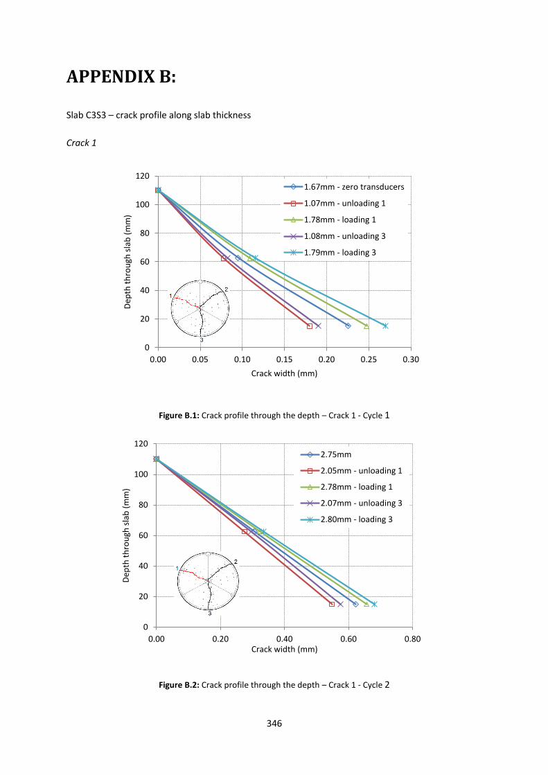
346
APPENDIX B:
Slab C3S3 – crack profile along slab thickness
Crack 1
Figure B.1: Crack profile through the depth – Crack 1 - Cycle 1
Figure B.2: Crack profile through the depth – Crack 1 - Cycle 2
0
20
40
60
80
100
120
0.00 0.05 0.10 0.15 0.20 0.25 0.30
Dep
th t
hro
ugh
sla
b (
mm
)
Crack width (mm)
1.67mm - zero transducers
1.07mm - unloading 1
1.78mm - loading 1
1.08mm - unloading 3
1.79mm - loading 3
0
20
40
60
80
100
120
0.00 0.20 0.40 0.60 0.80
Dep
th t
hro
ugh
sla
b (
mm
)
Crack width (mm)
2.75mm
2.05mm - unloading 1
2.78mm - loading 1
2.07mm - unloading 3
2.80mm - loading 3
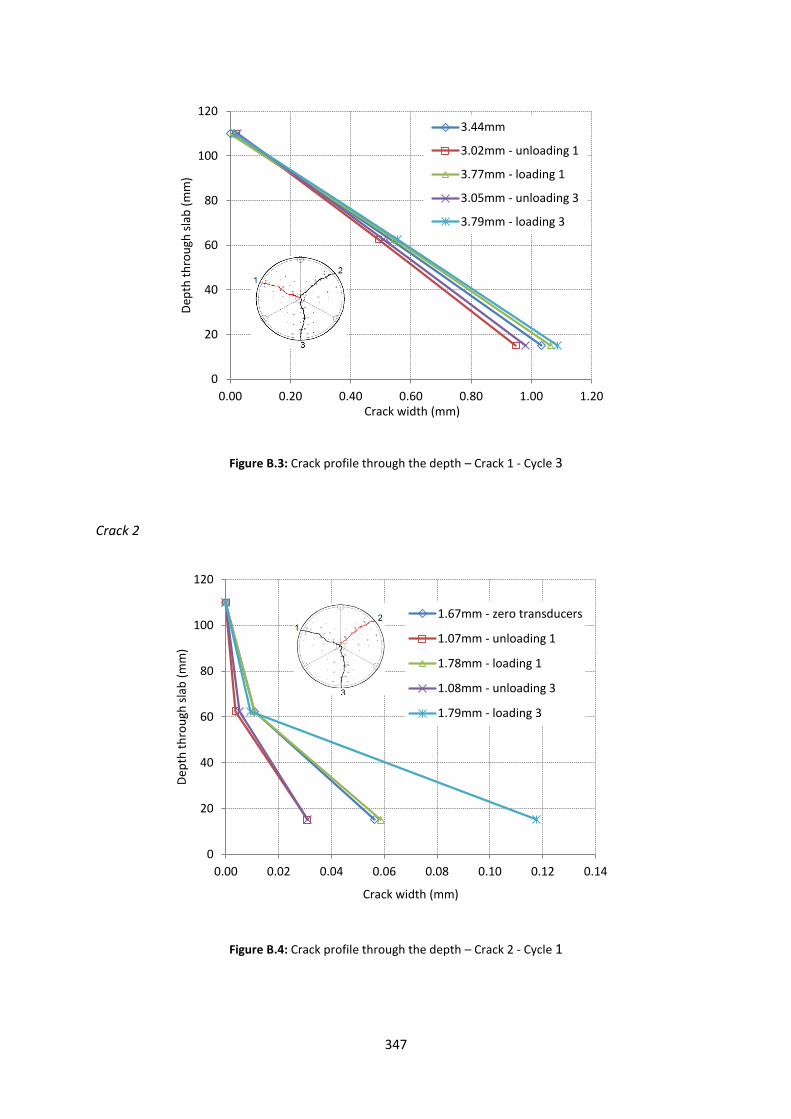
347
Figure B.3: Crack profile through the depth – Crack 1 - Cycle 3
Crack 2
Figure B.4: Crack profile through the depth – Crack 2 - Cycle 1
0
20
40
60
80
100
120
0.00 0.20 0.40 0.60 0.80 1.00 1.20
Dep
th t
hro
ugh
sla
b (
mm
)
Crack width (mm)
3.44mm
3.02mm - unloading 1
3.77mm - loading 1
3.05mm - unloading 3
3.79mm - loading 3
0
20
40
60
80
100
120
0.00 0.02 0.04 0.06 0.08 0.10 0.12 0.14
Dep
th t
hro
ugh
sla
b (
mm
)
Crack width (mm)
1.67mm - zero transducers
1.07mm - unloading 1
1.78mm - loading 1
1.08mm - unloading 3
1.79mm - loading 3
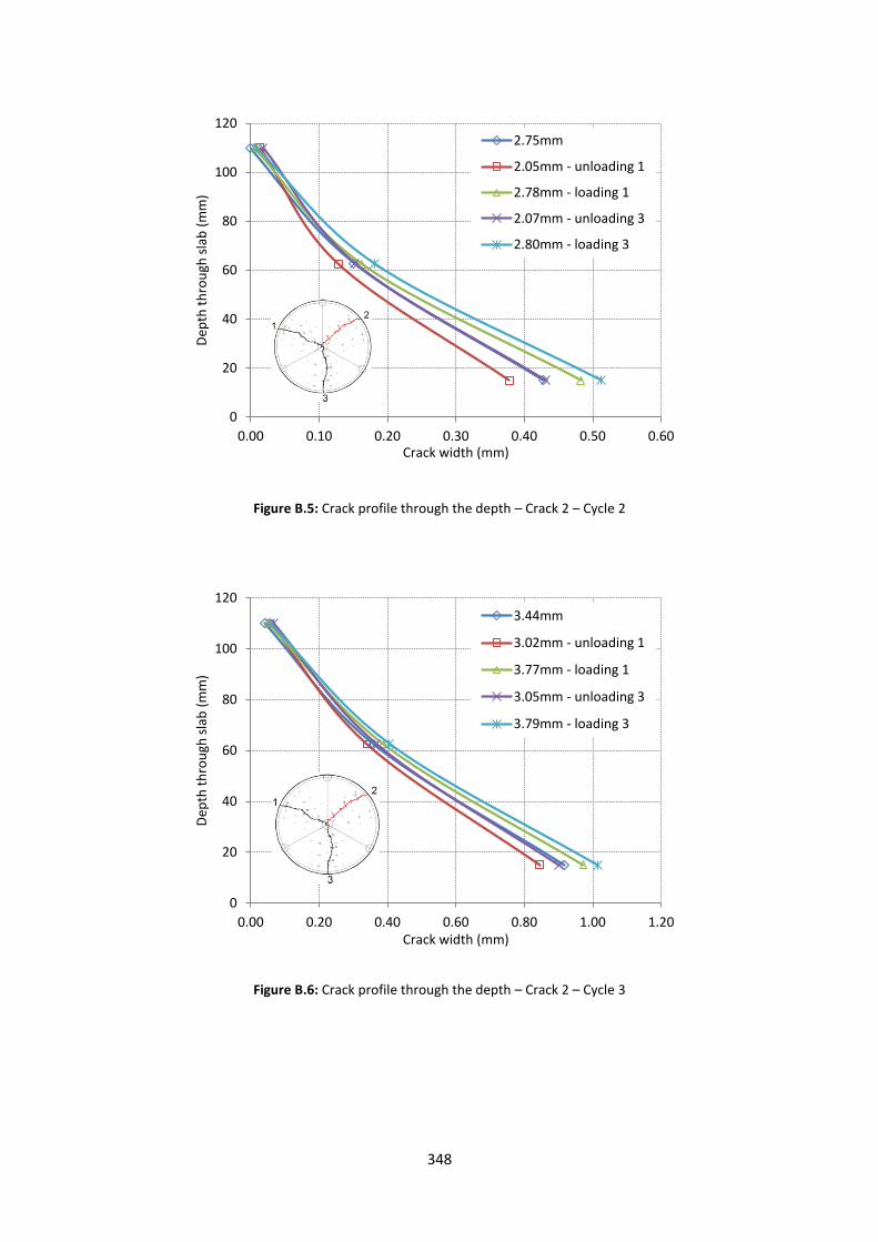
348
Figure B.5: Crack profile through the depth – Crack 2 – Cycle 2
Figure B.6: Crack profile through the depth – Crack 2 – Cycle 3
0
20
40
60
80
100
120
0.00 0.10 0.20 0.30 0.40 0.50 0.60
Dep
th t
hro
ugh
sla
b (
mm
)
Crack width (mm)
2.75mm
2.05mm - unloading 1
2.78mm - loading 1
2.07mm - unloading 3
2.80mm - loading 3
0
20
40
60
80
100
120
0.00 0.20 0.40 0.60 0.80 1.00 1.20
Dep
th t
hro
ugh
sla
b (
mm
)
Crack width (mm)
3.44mm
3.02mm - unloading 1
3.77mm - loading 1
3.05mm - unloading 3
3.79mm - loading 3
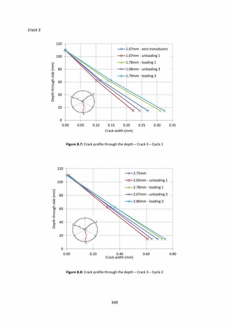
349
Crack 3
Figure B.7: Crack profile through the depth – Crack 3 – Cycle 1
Figure B.8: Crack profile through the depth – Crack 3 – Cycle 2
0
20
40
60
80
100
120
0.00 0.05 0.10 0.15 0.20 0.25 0.30 0.35
Dep
th t
hro
ugh
sla
b (
mm
)
Crack width (mm)
1.67mm - zero transducers
1.07mm - unloading 1
1.78mm - loading 1
1.08mm - unloading 3
1.79mm - loading 3
0
20
40
60
80
100
120
0.00 0.20 0.40 0.60 0.80
Dep
th t
hro
ugh
sla
b (
mm
)
Crack width (mm)
2.75mm
2.05mm - unloading 1
2.78mm - loading 1
2.07mm - unloading 3
2.80mm - loading 3

350
Figure B.9: Crack profile through the depth – Crack 3 – Cycle 3
0
20
40
60
80
100
120
0.00 0.20 0.40 0.60 0.80 1.00 1.20 1.40
Dep
th t
hro
ugh
sla
b (
mm
)
Crack width (mm)
3.44mm
3.02mm - unloading 1
3.77mm - loading 1
3.05mm - unloading 3
3.79mm - loading 3

351
APPENDIX C:
Strain profile through the depth
C3S1
Figure C.1: Strain profile through the depth – C3S1 – Crack 1
Figure C.2: Strain profile through the depth – C3S1 – Crack 2
0
20
40
60
80
100
120
0 0.001 0.002 0.003 0.004 0.005 0.006 0.007
Dep
th t
hro
ugh
sla
b (
mm
)
Total strain(mm)
1.87mm
2.20mm
2.61mm
3.69mm
4.93mm
0
20
40
60
80
100
120
0 0.0025 0.005 0.0075 0.01 0.0125
Dep
th t
hro
ugh
sla
b (
mm
)
Total strain(mm)
1.87mm
2.20mm
2.61mm
3.69mm
4.93mm
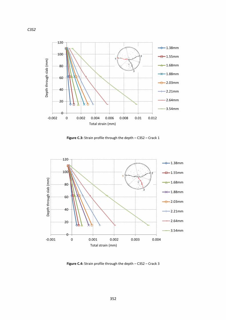
352
C3S2
Figure C.3: Strain profile through the depth – C3S2 – Crack 1
Figure C.4: Strain profile through the depth – C3S2 – Crack 3
0
20
40
60
80
100
120
-0.002 0 0.002 0.004 0.006 0.008 0.01 0.012
Dep
th t
hro
ugh
sla
b (
mm
)
Total strain (mm)
1.38mm
1.55mm
1.68mm
1.88mm
2.03mm
2.21mm
2.64mm
3.54mm
0
20
40
60
80
100
120
-0.001 0 0.001 0.002 0.003 0.004
Dep
th t
hro
ugh
sla
b (
mm
)
Total strain (mm)
1.38mm
1.55mm
1.68mm
1.88mm
2.03mm
2.21mm
2.64mm
3.54mm
Related Documents