BEAM EMBEDDED IN A WINKLER SOIL WITH ... - CIMEC

BEAM EMBEDDED IN A WINKLER SOIL WITH CLEARANCES.

ANALYTICAL SOLUTION OF THE NONLINEAL BENDING

PROBLEM.

Carlos P. Filipicha,b, Marta B. Rosalesb,c and Fernando S. Buezasc,d

aCIMTA, FRBB, Universidad Tecnológica Nacional, Bahía Blanca, Argentina, [email protected]

bDepartment of Engineering, Universidad Nacional del Sur, 8000 Bahía Blanca, Argentina,

[email protected]

cCONICET, Argentina

dDepartment of Physics, Universidad Nacional del Sur, 8000 Bahía Blanca, Argentina,

[email protected]

Keywords: beam, Winkler soil, clearances, drillstring

Abstract. The nonlinear bending problem of a beam embedded in a Winkler soil with clearances is

addressed by means of an analytical approach. This problem is of interest, for instance, in the study of

the drillstrings behavior under certain load conditions. Usually, a drillstring is modeled as a bar inside

an outer cylinder (bore-hole wall) with clearances that add strong nonlinearities. This work is part of a

wider study on drillstrings and a paper on the nonlinear vibration of this type of structure was presented in

ENIEF 2006. Here the title problem is simplified to a plane bar making contact with a Winkler-type soil.

The governing differential problem is derived using a minimal energy principle. The unknowns are the

lateral displacement due to bending (as usual) and the length of contact. The consideration of the latter

unknown leads to special restrictions among the admissible directions within the Calculus of Variation

deriving in a particular statement of the problem. Once the differential problem is fully established, a

solution of pairs of load-length of contact is found. Two particular examples are worked out: a cantilever

beam with a lateral tip load and a simply supported beam subjected to external end bending moments,

in both cases with several soil stiffness values. The numerical results are compared with a finite element

model. The availability of an analytical approach permits the calibration of other numerical solutions,

e.g. the study of convergences issues. On the other hand other complexities, such as the consideration of

axial loads including self-weight that leads to the inclusion of the second order effect, are under study at

present.

Mecánica Computacional Vol XXVIII, págs. 1797-1807 (artículo completo)Cristian García Bauza, Pablo Lotito, Lisandro Parente, Marcelo Vénere (Eds.)

Tandil, Argentina, 3-6 Noviembre 2009

Copyright © 2009 Asociación Argentina de Mecánica Computacional http://www.amcaonline.org.ar

1 INTRODUCTION

The title problem is of interest when studying the beam-columns (typically drillstrings) struc-

tural behavior. One of the possible states deals with loads leading to lateral displacements of a

beam inside a hole surrounded by soil. The present work is part of a wider study on drillstrings

and a paper on the nonlinear vibration of this type of structure was presented in ENIEF 2006

Filipich et al. (2006). The Winkler soil model has been object of wide research. An interesting

review (Dutta and Roy, 2002) deals with the simpler and more complex models employed in

the study of soil-structures problems. A recent paper by ElGanainy and ElNaggar (2009) deals

with a nonlinear Winkler foundation model and Silveira et al. (2008) tackle the equilibrium

and stability of structural elements under unilateral constraints using a Ritz type approach. A

simplified approach may be tackled by means of a Winkler elastic soil model. The authors

have used this model to address some beam dynamic problems (Filipich and Rosales, 1988,

2002; Filipich et al., 2006). Despite the simplicity of the problem, certain peculiarities arise, in

the present study, in the derivation of the governing equations within the Calculus of Variation

regarding with the variable limits of the contact. Also, the clearances are responsible of a non-

linear response. Some parts of the beams will be in contact with the soil while others remain

inside the hole. The length of the contact region is, at first, unknown for a given load state.

The governing equations and the boundary conditions are derived and special care should be

taken to consider the existence of integration limits that are functions of the independent vari-

able. Even in the range of small deformations and under linear elastic behavior of the material,

unilateral constraints lead to highly nonlinear responses. The problem will be stated for two

different configurations, a cantilever beam with a transverse tip load and a simply supported

beam with bending external moments at the ends. Finally numerical examples will be presented

to illustrate the problem and comparison with finite element results also included.

2 STATEMENT OF THE PROBLEM: BEAM IN A BORE-HOLE SURROUNDED BY

A WINKLER-TYPE SOIL.

In this Section, the governing differential system of a beam inserted in a hole which is sur-

rounded by a Winkler-type soil is stated. Two different configurations will be studied, i.e. a

uniform cantilever beam with a transverse load P and a simply supported beam subjected to

external end bending moments.

2.1 Uniform cantilever beam with a transverse load P .

Let the total static energy U∗ of the beam with a lateral displacement due to a lateral tip load

and considering the existence of clearance ε (see Figure 1), be

2U∗[v1; v2; a] = EJ

{∫ a

0

v21xxdX +

k0

EJ

∫ a

0

(v1 − ε)2dX+

∫ L

a

v22xxdX − 2P

EJv1(0)

}

(1)

(0 ≤ X ≤ L)

where vj = vj(X), j = 1, 2, a = a(X), E is the Young’s modulus, J is the moment of inertia,

P is the lateral load and k0 is the Winkler soil constant. The equilibrium condition is

δU∗ = 0 (2)

C.P. FILIPICH, M.B. ROSALES, F.S. BUEZAS1798


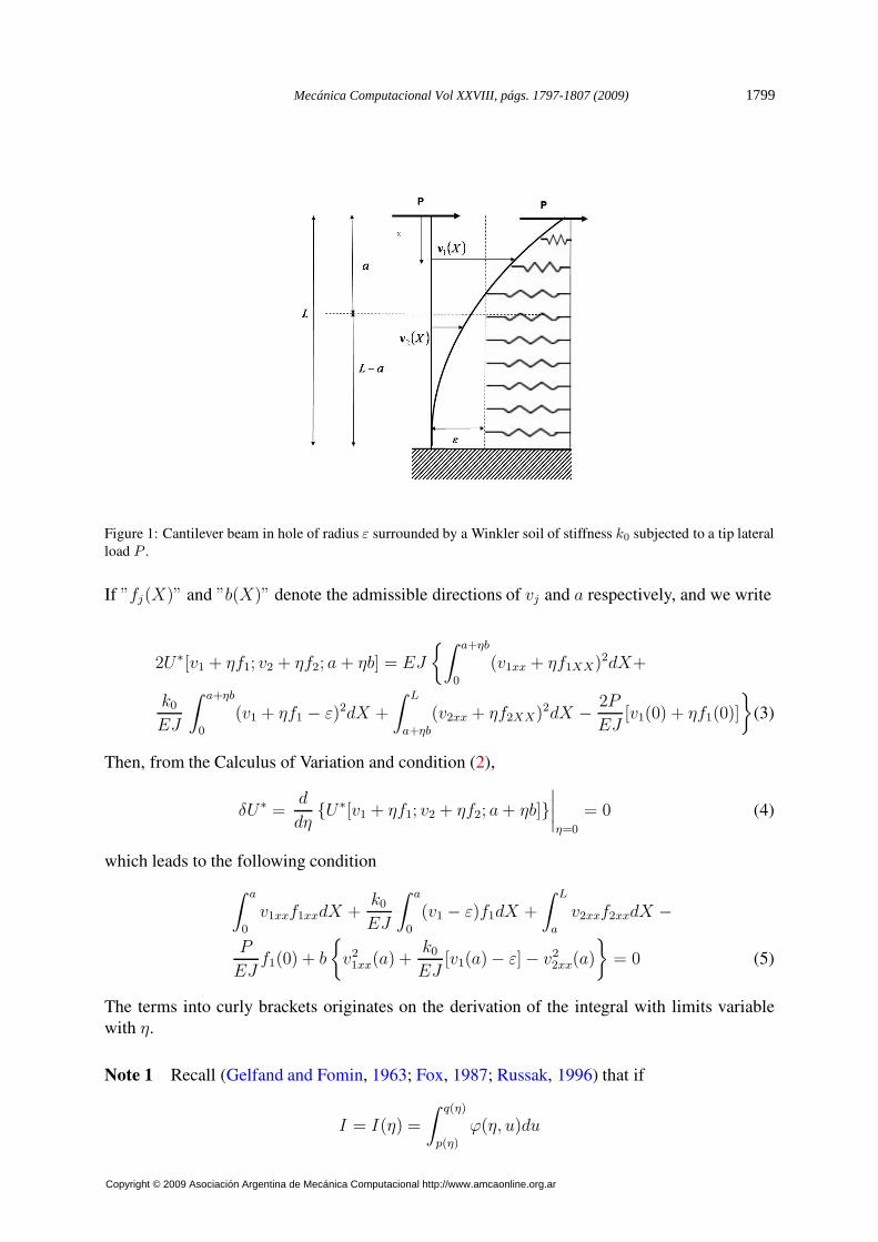
Figure 1: Cantilever beam in hole of radius ε surrounded by a Winkler soil of stiffness k0 subjected to a tip lateral

load P .

If ”fj(X)” and ”b(X)” denote the admissible directions of vj and a respectively, and we write

2U∗[v1 + ηf1; v2 + ηf2; a + ηb] = EJ

{∫ a+ηb

0

(v1xx + ηf1XX)2dX+

k0

EJ

∫ a+ηb

0

(v1 + ηf1 − ε)2dX +

∫ L

a+ηb

(v2xx + ηf2XX)2dX − 2P

EJ[v1(0) + ηf1(0)]

}

(3)

Then, from the Calculus of Variation and condition (2),

δU∗ =d

dη{U∗[v1 + ηf1; v2 + ηf2; a + ηb]}

∣

∣

∣

∣

η=0

= 0 (4)

which leads to the following condition

∫ a

0

v1xxf1xxdX +k0

EJ

∫ a

0

(v1 − ε)f1dX +

∫ L

a

v2xxf2xxdX −

P

EJf1(0) + b

{

v21xx(a) +

k0

EJ[v1(a)− ε] − v2

2xx(a)

}

= 0 (5)

The terms into curly brackets originates on the derivation of the integral with limits variable

with η.

Note 1 Recall (Gelfand and Fomin, 1963; Fox, 1987; Russak, 1996) that if

I = I(η) =

∫ q(η)

p(η)

ϕ(η, u)du

Mecánica Computacional Vol XXVIII, págs. 1797-1807 (2009) 1799


then the derivative of the integral w.r.t. η is

Iη =dI(η)

dη=

∫ q(η)

p(η)

ϕη(η, u)du + ϕ(η, q(x))qx(x) − ϕ(η, p(x))px(x).

Before working with Eq. (5), let us impose the conditions for the geometrical continuity (com-

patibility of deformation conditions) at a

v1(a) = ε (6a)

v2(a) = ε (6b)

v1X(a) = v2X(a) (6c)

Now, before the integration by parts of Eq. (5), it will be necessary to know, among other

variations, fj(a) and fjX(a), j = 1, 2 (variations of the function and the first derivative, re-

spectively) which deserves an special detail. In effect, if we write, for instance, the following

equalities:

v1(a) ≡ F1[v1; a] ≡ 1

a

∫ a

0

v1(a)dX (7a)

v2(a) ≡ F2[v2; a] ≡ 1

L − a

∫ L

a

v2(a)dX (7b)

The definitions of the "functionals" F1[vj, a] permits to express the following variations:

δvj(a) =d

dη{Fj[vj + ηfj ; a + ηb]}

∣

∣

∣

∣

η=0

(j = 1, 2) (8)

where, for instance, the variation of F1 writes

F1[v1 + ηf1; a + ηb] =1

a + ηb

∫ a+ηb

0

[v1(a + ηb) + ηf1(a + ηb)]dX.

The following relevant conclusions are derived:

δvj(a) = fj(a) + vjX(a)b (9)

δvjX(a) = fjX(a) + vjXX(a)b (10)

NOTE 2 It could be thought at first that according to conditions (6a) and (6b) and with v1(a)and v2(a) already imposed, then one should conclude that f1(a) = f2(a) = 0, which is erro-

neous, as is now demonstrated. If the latter were used, wrong boundary conditions would be

obtained. From Eqs. (6)

δvj(a) = 0 (j = 1, 2) (11a)

δv1X(a) = δv2X(a) (11b)

with which, after using results (9) and (10), one obtains

fj(a) = −vjX(a)b (j = 1, 2) (12a)

f2X(a) = f1X(a) + b[v1XX(a) − v2XX(a)]. (12b)



Now, integrating by parts Eq. (5) and taking into account (6a), the following expression is

obtained

∫ a

0

[

v1XXXX +k0

EJ(v1 − ε)

]

f1dX +

∫ L

a

v2XXXX f2dX +

|v1XX f1X|a0 − |v1XXX f1|a0 − P f1(0) + |v2XX f2X|La −|v2XXX f2|La + b[v2

1XX(a) − v22XX(a)] = 0 (13)

On the other hand, when dealing with a cantilever, two stable or geometric boundary conditions

have to be fulfilled

v2(L) = 0 (14a)

v2X(L) = 0 (14b)

that, in this case, give place to

f2(L) = f2X(L) = 0 (15)

After accepting that the variations fj(X) and their derivatives are independents from the Funda-

mental Theorem of the Calculus of Variation, and considering (9), (10) and (15), we arrive to the

conclusion that the equilibrium (13) is equivalent to the fulfillment of the following equations

v1XXXX +k0

EJ(v1 − ε) = 0 (16a)

v2XXXX = 0 (16b)

v1XX(0)f1(0) = 0 (16c)[

v1XXX(0) − P

EJ

]

f1(0) = 0 (16d)

[v1XX(a) − v2XX(a)] f1X(0) = 0 (16e)

{[v1XXX(a)− v2XXX(a)] v1X(a) + [v1XX(a) − v2XX(a)] v1XX(a)} b = 0 (16f)

As may be observed, the DE (16a) and (16b) and the natural boundary conditions at X = 0 and

the continuity ones at X = a, must be fulfilled. Meanwhile, conditions (16c-16e) would appear

commonly in a domain arbitrary divided at X = a, with k0 = 0. Eq. (16f) is not apparent.

Anyway, in the present case of the cantilever beam, in general, v1(0) 6= 0 and v1X(0) 6= 0 and

consequently, f1(0) 6= 0 and f1X(0) 6= 0. Also, in general, v1X(a) 6= 0 and then, due to Eqs. (6)

and (12b), f1X(a) 6= 0 as well as b 6= 0 (it has not to be assumed null in general). Additionally

with the above- mentioned and, from (16), the following should be satisfied,

v1XX(0) = 0 (17a)

v1XXX(0) =P

EJ(17b)

v1XX(a) = v2XX(a) (17c)

v1XXX(a) = v2XXX(a) (17d)

Equations (17) together with Eqs. (6) and (14) yield the nine boundary and continuity conditions

for this problem.



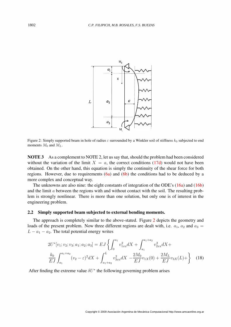
Figure 2: Simply supported beam in hole of radius ε surrounded by a Winkler soil of stiffness k0 subjected to end

moments M0 and ML .

NOTE 3 As a complement to NOTE 2, let us say that, should the problem had been considered

without the variation of the limit X = a, the correct conditions (17d) would not have been

obtained. On the other hand, this equation is simply the continuity of the shear force for both

regions. However, due to requirements (6a) and (6b) the conditions had to be deduced by a

more complex and conceptual way.

The unknowns are also nine: the eight constants of integration of the ODE’s (16a) and (16b)

and the limit a between the regions with and without contact with the soil. The resulting prob-

lem is strongly nonlinear. There is more than one solution, but only one is of interest in the

engineering problem.

2.2 Simply supported beam subjected to external bending moments.

The approach is completely similar to the above-stated. Figure 2 depicts the geometry and

loads of the present problem. Now three different regions are dealt with, i.e. a1, a2 and a3 =L − a1 − a2. The total potential energy writes

2U∗[v1; v2; v3; a1; a2; a3] = EJ

{∫ a1

0

v21xxdX +

∫ a1+a2

a1

v22xxdX+

k0

EJ

∫ a1+a2

a1

(v2 − ε)2dX +

∫ L

a1+a2

v23xxdX −2M0

EJv1X(0) +

2ML

EJv3X(L)+

}

(18)

After finding the extreme value δU∗ the following governing problem arises



v1XXXX = 0 (19a)

v2XXXX +k0

EJ(v2 − ε) = 0 (19b)

v3XXXX = 0 (19c)

v1(0) = 0; v3(L) = 0; (19d)

v1(a1) = ε; v2(a1) = ε; v2(a1 + a2) = ε; v3(a1 + a2) = ε; (19e)

v1X(a1) = v2X(a1); v2X(a1 + a2) = v3X(a1 + a2); (19f)

v1XX(0) =M0

EJ; v3XX(L) = 0; (19g)

v1XX(a1) = v2XX(a1); v2XX(a1 + a2) = v3XX(a1 + a2); (19h)

v1XXX(a1) = v2XXX(a1); v2XXX(a1 + a2) = v3XXX(a1 + a2); (19i)

Then, there are 14 unknowns —12 integration constants and the contact lengths a1 and a2 and

14 boundary and continuity conditions (19d-19i), that make this nonlinear problem consistent.

3 CANTILEVER BEAM: SOLUTION OF THE DIFFERENTIAL SYSTEM

Now let us tackle the solution of the differential problem stated in Eqs. (16-17). Let us

consider that the contact length a is fixed, i.e. assumed known for each equilibrium solution.

Let us introduce the next notation

0 ≤ X ≤ a; x1 =X

a⇒ 0 ≤ x1 ≤ 1; a ≤ X ≤ L; x2 =

X − a

L − a⇒ 0 ≤ x2 ≤ 1;

Also if k4 = k0a4/(EJ) and p = Pa3/(EJ) the following equations yield

v′′′′

1 + k4v1 = k4εv′′

1(0) = 0; v′′′

1 (0) = p;

}

with (·)′ =d(·)dx1

(20)

v′′′′

2 = 0v2(1) = 0; v′

2(0) = 0;

}

with (·)′ =d(·)dx2

(21)

v1(1) = 0; v2(0) = 0; (22a)

v2(0) = ε; (22b)

L − a

av′

1(1) = v′

2(0); (22c)

(L − a)2

a2v′′

1(1) = v′′

2(0); (22d)

(L − a)3

a

3

v′′′

1 (1) = v′′′

2 (0). (22e)

The solutions of the two unknowns v1(x1) and v1(x2) with λ ≡ k/√

2 = 4

√

k0/(4EJ), write

v1(x1) = ε + sinhλx1 (A1 sinλx1 + A2 cos λx1)

+ cosh λx1 (A3 sinλx1 + A4 cosλx1) (23)

v2(x2) = B1 + B2x2 + B3x22 + B4x

32 (24)



3.1 Practical algorithm to solve the cantilever case

From (20) (second row, left condition), one finds A1 = 0 and using (22b), B1 = ε. Given the

data L, ε, E, k0 and J , equations (21) and (22) will be used to find {A2 A3 A4 B2 B3 B4},

but functionally depending on the parameter a (not as function of x). From (20),

p = p(a) = v′′′

1 (0) ⇒ P = P (a) =pEJ

a3(25)

If the applied load P = P0 is assumed known, then the root a of

P0 −p(a)EJ

a3= 0 (26)

is no more than the sought solution a for each P0, if a solution exists.

4 SIMPLY SUPPORTED BEAM: SOLUTION OF THE DIFFERENTIAL SYSTEM

The methodology is completely analogous to the above described. Let us consider the con-

figuration of Figure 2 and that the contact lengths a1 and a3 are fixed, i.e. assumed known for

each equilibrium solution. The solutions are now divided in three spans, The solutions of the

two unknowns v1(x1) and v1(x2) with λ ≡ k/√

2 = 4

√

k0/(4EJ), write

v1(x1) = A1 + A2x1 + A3x21 + A4x

31 (27)

v2(x2) = ε + sinhλx2 (B1 sinλx2 + B2 cos λx2)

+ cosh λx2 (B3 sinλx2 + B4 cos λx2) (28)

v3(x3) = C1 + C2x3 + C3x23 + C4x

33 (29)

where x1 = X/a1, x2 = (X − a1)/a2, x3 = [X − (a1 + a2)]/a3, λ = a24

√

k0/(4EJ) and

a1 + a2 + a3 = L. It is accepted that a1 and a3 are fixed and considered as parameters.

v1(x1), v1(x2) and v3(x3) are found from solving Eqs. (19a-22c) (after non-dimensionalization).

Boundary and continuity conditions (19d-19i) after non-dimensionalization yield (with r1 ≡a2/a1 and r1 ≡ a2/a1)

v1(1) = 0; v2(0) = ε; v3(0) = ε; (30a)

v1(1) = v2(0) (30b)

v2(1) = v3(0) (30c)

r1v′

1(1) = v′

2(0) (30d)

r2v′

2(1) = v′

3(0) (30e)

v′′

1(0) = −m0 ≡ −M0a21

EJ(30f)

r21v

′′

1(1) = v′′

2(0) (30g)

r22v

′′

2(1) = v′′

3(0) (30h)

v′′

2(1) = −mL ≡ −MLa23

EJ(30i)

r31v

′′′

1 (1) = v′′′

2 (0) (30j)

r33v

′′′

2 (1) = v′′′

3 (0) (30k)

v3(1) = 0 (30l)



4.1 Practical algorithm to solve the simply supported case.

From conditions (30a), A1 = 0, B4 = 0 and C1 = ε are respectively found. Given the data L,

ε, E, k0 and J , equations (30b-30e), (30g-30h) and (30j-30l), {A2 A3 A4 B1 B2 B3 C2 C3 C4}yield. They functionally depend on the parameters a1 and a3 (⇒ a2 = L − (a1 + a3)) (not as

function of x). A highly nonlinear system of equations is obtained: two equations (30f) and

(30i)with two unknowns m0(a1, a3) and mL(a1, a3), i.e.

M0 = M0(a1, a3) =EJ

a21

m0(a1, a3) (31)

ML = ML(a1, a3) =EJ

a23

mL(a1, a3) (32)

As before, if the applied moments M0 and ML are assumed known, then the values of a1 and

a3 (if a solution exists) arise from the following nonlinear system:

M0 −m0(a1, a3)EJ

a21

= 0 (33)

ML − mL(a1, a3)EJ

a23

= 0. (34)

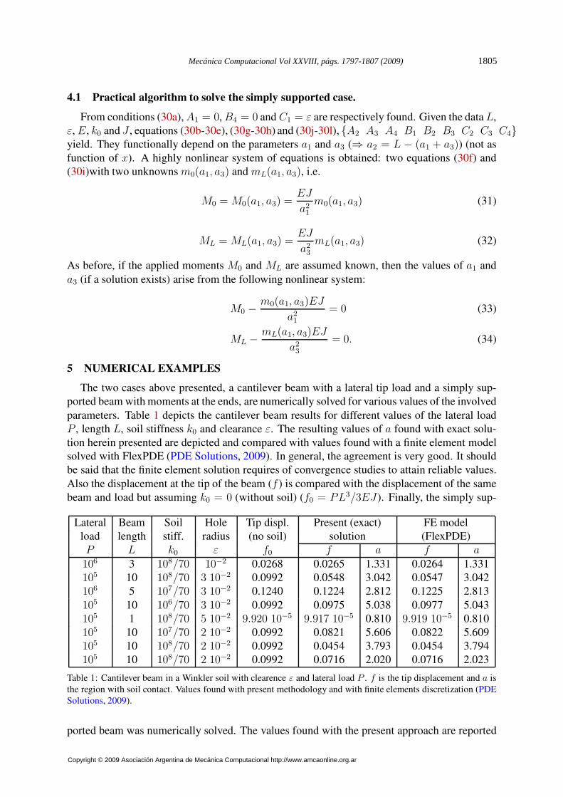
5 NUMERICAL EXAMPLES

The two cases above presented, a cantilever beam with a lateral tip load and a simply sup-

ported beam with moments at the ends, are numerically solved for various values of the involved

parameters. Table 1 depicts the cantilever beam results for different values of the lateral load

P , length L, soil stiffness k0 and clearance ε. The resulting values of a found with exact solu-

tion herein presented are depicted and compared with values found with a finite element model

solved with FlexPDE (PDE Solutions, 2009). In general, the agreement is very good. It should

be said that the finite element solution requires of convergence studies to attain reliable values.

Also the displacement at the tip of the beam (f) is compared with the displacement of the same

beam and load but assuming k0 = 0 (without soil) (f0 = PL3/3EJ ). Finally, the simply sup-

Lateral Beam Soil Hole Tip displ. Present (exact) FE model

load length stiff. radius (no soil) solution (FlexPDE)

P L k0 ε f0 f a f a106 3 108/70 10−2 0.0268 0.0265 1.331 0.0264 1.331

105 10 108/70 3 10−2 0.0992 0.0548 3.042 0.0547 3.042

106 5 107/70 3 10−2 0.1240 0.1224 2.812 0.1225 2.813

105 10 106/70 3 10−2 0.0992 0.0975 5.038 0.0977 5.043

105 1 108/70 5 10−2 9.920 10−5 9.917 10−5 0.810 9.919 10−5 0.810

105 10 107/70 2 10−2 0.0992 0.0821 5.606 0.0822 5.609

105 10 108/70 2 10−2 0.0992 0.0454 3.793 0.0454 3.794

105 10 108/70 2 10−2 0.0992 0.0716 2.020 0.0716 2.023

Table 1: Cantilever beam in a Winkler soil with clearence ε and lateral load P . f is the tip displacement and a is

the region with soil contact. Values found with present methodology and with finite elements discretization (PDE

Solutions, 2009).

ported beam was numerically solved. The values found with the present approach are reported



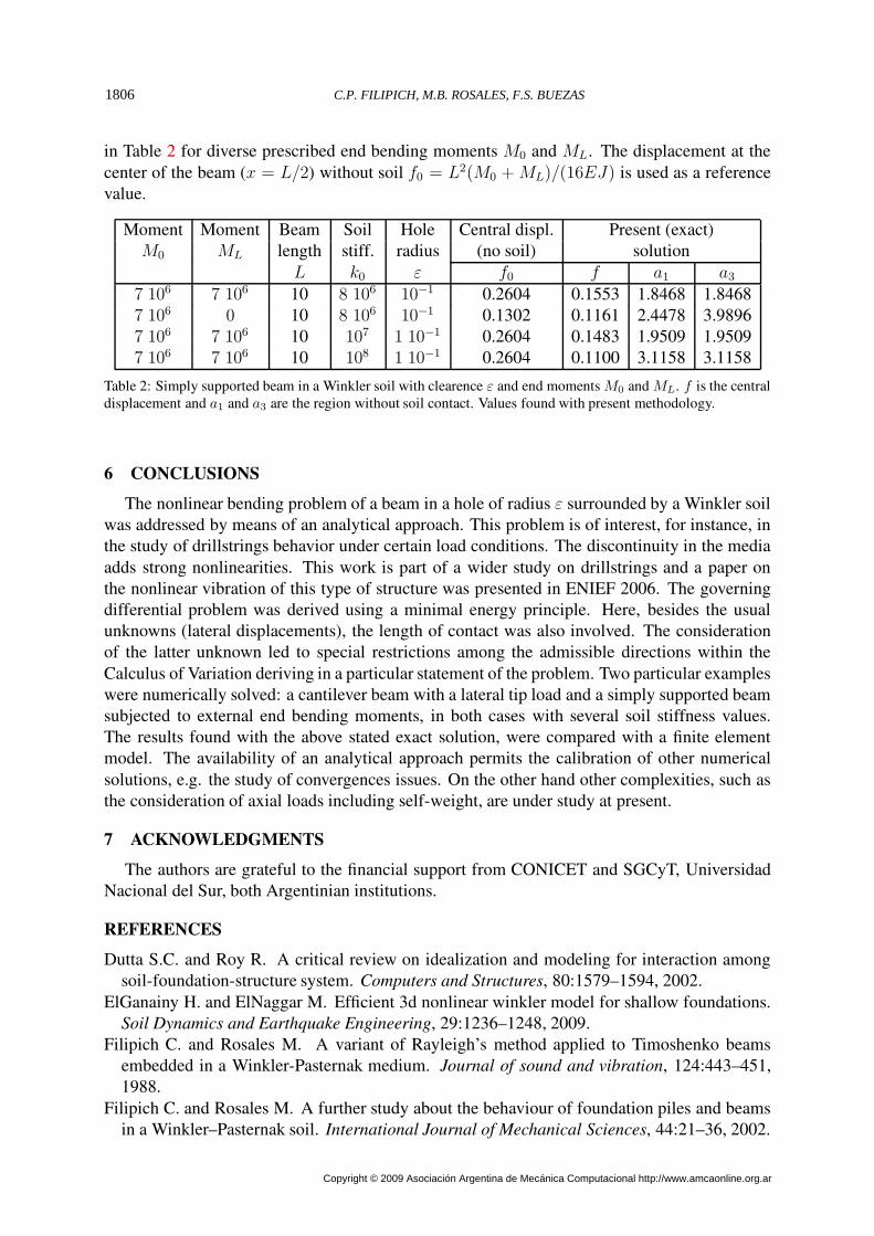
in Table 2 for diverse prescribed end bending moments M0 and ML. The displacement at the

center of the beam (x = L/2) without soil f0 = L2(M0 + ML)/(16EJ) is used as a reference

value.

Moment Moment Beam Soil Hole Central displ. Present (exact)

M0 ML length stiff. radius (no soil) solution

L k0 ε f0 f a1 a3

7 106 7 106 10 8 106 10−1 0.2604 0.1553 1.8468 1.8468

7 106 0 10 8 106 10−1 0.1302 0.1161 2.4478 3.9896

7 106 7 106 10 107 1 10−1 0.2604 0.1483 1.9509 1.9509

7 106 7 106 10 108 1 10−1 0.2604 0.1100 3.1158 3.1158

Table 2: Simply supported beam in a Winkler soil with clearence ε and end moments M0 and ML. f is the central

displacement and a1 and a3 are the region without soil contact. Values found with present methodology.

6 CONCLUSIONS

The nonlinear bending problem of a beam in a hole of radius ε surrounded by a Winkler soil

was addressed by means of an analytical approach. This problem is of interest, for instance, in

the study of drillstrings behavior under certain load conditions. The discontinuity in the media

adds strong nonlinearities. This work is part of a wider study on drillstrings and a paper on

the nonlinear vibration of this type of structure was presented in ENIEF 2006. The governing

differential problem was derived using a minimal energy principle. Here, besides the usual

unknowns (lateral displacements), the length of contact was also involved. The consideration

of the latter unknown led to special restrictions among the admissible directions within the

Calculus of Variation deriving in a particular statement of the problem. Two particular examples

were numerically solved: a cantilever beam with a lateral tip load and a simply supported beam

subjected to external end bending moments, in both cases with several soil stiffness values.

The results found with the above stated exact solution, were compared with a finite element

model. The availability of an analytical approach permits the calibration of other numerical

solutions, e.g. the study of convergences issues. On the other hand other complexities, such as

the consideration of axial loads including self-weight, are under study at present.

7 ACKNOWLEDGMENTS

The authors are grateful to the financial support from CONICET and SGCyT, Universidad

Nacional del Sur, both Argentinian institutions.

REFERENCES

Dutta S.C. and Roy R. A critical review on idealization and modeling for interaction among

soil-foundation-structure system. Computers and Structures, 80:1579–1594, 2002.

ElGanainy H. and ElNaggar M. Efficient 3d nonlinear winkler model for shallow foundations.

Soil Dynamics and Earthquake Engineering, 29:1236–1248, 2009.

Filipich C. and Rosales M. A variant of Rayleigh’s method applied to Timoshenko beams

embedded in a Winkler-Pasternak medium. Journal of sound and vibration, 124:443–451,

1988.

Filipich C. and Rosales M. A further study about the behaviour of foundation piles and beams

in a Winkler–Pasternak soil. International Journal of Mechanical Sciences, 44:21–36, 2002.



Filipich C., Rosales M., and Sampaio R. Semi-analytical solution of non-linear vibration of

beams with clearances consideration. In Mecánica Computacional, volume XXV, pages

1781–1792. 2006.

Fox C. An introduction to the calculus of variations. Dover Editions, 1987.

Gelfand I. and Fomin S. Calculus of variations. Revised English edition translated and edited

by Richard A. Silverman. Prentice-Hall, Inc., Englewood Cliffs, NJ, 1963.

PDE Solutions. FlexPDE V.6 Manual, 2009.

Russak I. Calculus of variations : MA 4311 lecture notes . Department of Mathematics, Naval

Postgraduate School, Code MA/Ru, Monterey, California, USA, 1996.

Silveira R.A., Pereira W.L., and Goncalves P.B. Nonlinear analysis of structural elements under

unilateral contact constraints by a Ritz type approach. International Journal of Solids and

Structures, 45:2629–2650, 2008.



BEAM EMBEDDED IN A WINKLER SOIL WITH ... - CIMEC

Documents