BDI-modelling of complex intracellular dynamics

1

BDI-Modelling of Complex Intracellular Dynamics C.M. Jonker1, J.L. Snoep2,4, J. Treur1,

H.V. Westerhoff3,4 and W.C.A. Wijngaards1 1Vrije Universiteit Amsterdam, Department of Artificial Intelligence,

De Boelelaan 1081a, NL-1081 HV Amsterdam, The Netherlands, EU, {jonker, treur, wouterw}@cs.vu.nl 2University of Stellenbosch, Department of Biochemistry, Private Bag X1,

Matieland 7602, Stellenbosch, South Africa, [email protected] 3Stellenbosch Institute for Advanced Study, South Africa and

4BioCentrum Amsterdam, Department of

Molecular Cell Physiology, De Boelelaan 1087, NL-1081 HV Amsterdam, The Netherlands, EU, [email protected]

ABSTRACT A BDI-based continuous-time modelling approach for intracellular dynamics is presented. It is shown how temporalised BDI-models make it possible to model intracellular biochemical processes as decision processes. By abstracting from some of the details of the biochemical pathways, the model achieves understanding in nearly intuitive terms, without losing veracity: classical intentional state properties such as Beliefs, Desires and Intentions, are founded in reality through precise biochemical relations. In an extensive example, the complex regulation of Escherichia coli vis-à-vis lactose, glucose and oxygen is simulated as a discrete-state, continuous-time temporal decision manager. Thus a bridge is introduced between two different scientific areas: the area of BDI-modelling and the area of intracellular dynamics.

Keywords modelling of bacterial behavior, continuous time, intentional, BDI-model, catabolite repression, regulation

1. INTRODUCTION Even the simplest life forms require the interaction of more than 400 chemical processes that are encoded by genes [Hutchison et al., 1999]. The sequencing of many complete genomes should bring cell biochemistry to full fruition, at last: efforts can now be directed at clarifying the dynamic functioning of genes within the ensemble of cellular processes. But how should one manage and understand hundreds of biochemical processes simultaneously? After ages of qualitative or quasi-quantitative modelling, a mathematical biochemistry approach is coming within reach (Westerhoff, 2001). The biochemical processes are described by the appropriate differential or algebraic equations, the parameter values are taken from experimental studies, and are integrated numerically (e.g. Mendes, 1997). For some unicellular organisms such as the bacterium Escherichia coli (Rohwer et al., 2000, Wang et al., 2001, Tomita et al., 1999, cf. Ben-Jacob et al., 1997), the yeast S. cerevisiae (Teusink et al., 2000; Rizzi et al., 1997), D. discoideum (Wright and Albe, 1994) and T. brucei (Bakker et al., 1997), and for the red blood cell (Mulquiney and Küchel, 1999) some of the chemical pathways are understood in sufficient kinetic detail to obtain a description of their import and primary processing of glucose.

As close to the aims of our scientific endeavor as this approach may seem to be, it does have major limitations: (1) Even for relatively short biochemical pathways, a

hundred or more reaction parameters are needed, which have rarely been determined under the appropriate experimental conditions (e.g. Teusink et al., 2000). (2) Due to non-linearities in the dynamics, results can depend strongly on parameter values, such that simple estimates may not suffice. (3) Biochemical pathways are integrated with other pathways, including ones of signal transduction and gene expression, for which reliable parameter estimates are even rarer [Kholodenko et al., 1999]. (4) It is still unclear whether parameter values determined in

vitro are relevant in vivo [Visser et al., 2000; Rohwer et

al. 1998]. (5) Actual behavior of intracellular pathways may be much less complex than possible in principle on the basis of their complexity (e.g. Van Rotterdam et al., 2002). (6) At best approaches those referred to above deliver a computer replica of (part of) the living cell, which is almost as remote from human understanding, as the cell itself; this modelling approach gives too detailed and complex an account, where the human mind tends to focus, after understanding, merely on the essence of the system.

Indeed, in order to grasp the workings of the cell, approaches abstracting from biochemical detail might be helpful. One type of such approaches focuses on a particular facet of cell function, such as its energetics, control, performance, optimisation, type of dynamics, or flux distributions (Westerhoff and Van Dam, 1987; Heinrich and Schuster, 1996; Moller et al., 2002) thereby allowing substantial approximations to rate equations. A second type recognizes that some conglomerates of biochemical processes act as functional units such as “metabolic pathway”, “catabolism”, “transcriptome” and “regulon”. Some of these concepts have been or are being defined formally (Kahn & Westerhoff, 1991; Rohwer et al., 1996b; Schilling et al., 2000), but optimal implementation is still in its infancy. A third type of approach recognizes a less than full complexity in cell functioning, for instance in the limited dimensionality of the transcriptome, or the metabolome. Indeed, viewed from the functional side, the cell effectively makes decisions regarding its internal and externally observable behavior, given its environmental circumstances, and implements these decisions into appropriate actions. The exact time it takes to make these decisions, and hence the precise integration of the differential equations, may be much less important than the fact that the decision is

2

taken within some reasonable time interval. This suggests that considering a cell from the perspective of an agent sensing the environment, integrating that information with its internal state, and then choosing between possible behavioural patterns of action, may provide the basis of an alternative modelling approach.

Within the field of Artificial Intelligence, the area of Agent Systems addresses the modelling of artificial and natural decision makers. One sort of these agent models are BDI-models describing agents in terms of internal state properties such as Beliefs, Desires and Intentions (e.g., Rao and Georgeff, 1991; Jonker, Treur and Wijngaards, 2003). In (Jonker, Snoep, Treur, Westerhoff, and Wijngaards, 2002) the BDI-modelling approach is used to identify and analyse steady states within the cell in relation to environmental circumstances. The BDI-models available in the literature do not adequately address the dynamics of the internal state properties over time, nor do they specify in which order and at what time the appropriate beliefs, desires and intentions are generated in relation to environmental conditions. Since Jonker et al. (2002) dealt with steady states, this limitation of the BDI-model was harmless, and relating the steady states to different environmental circumstances fitted well to the logic of the BDI-modelling strategy which abstracts from internal dynamics.

A main problem to be addressed in non-steady dynamics, is to characterise for changing environmental conditions, what internal dynamics realise the transitions over time from one steady state to another. The dynamics become even less trivial when the environment is changing continuously so that the cell never reaches any steady state. An underlying fundamental problem is how to relate discrete, binary decision processes to continuous

dynamics over time as occurring in the biochemical reaction network.

To model agents, often methods originating from some variant of temporal logic are used; see (Galton, 2003, 2006) for an overview. In agent simulation models, time is often chosen to be discrete and dynamics is based on step by step state transitions from one discrete point in time to the next (e.g., Sloman and Poli, 1995; the Executable Temporal Logic of Barringer et al. 1996 and Fisher, 1994, 2005; the step-logic of Elgot-Drapkin and Perlis, 1990). These discrete modelling approaches do not fully capture the continuous dynamics of processes in the real world, which is the basis of, for example, the internal dynamics of cellular processes.

For the analysis of concurrent real-time processes, also some temporal requirement specification languages have been introduced; e.g., (Dardenne et al., 1993; Darimont and Lamsweerde, 1996; Dubois et al., 1995). In (Chaochen, Hoare, and Ravn, 1991) a calculus is presented to model requirements and designs for real-time systems. Another logic based approach using time durations is presented in (Sandewall, 1997). These approaches can be used for analysis of dynamics but are not aimed at simulation.

The current paper addresses the problem of continuous versus discrete time in yet another way. It is shown how the BDI-model can be extended or temporalised by adding a (continuous, real time) temporal dimension for the internal dynamics of the beliefs, desires and intentions over time (cf. Finger and Gabbay, 1992). It is shown that this temporalised Continuous Time BDI-model, the CTBDI-model in short, covers the (non-steady state) dynamics of a cell’s biochemical pathways. By using the CTBDI-model to describe the cell’s internal processes in terms of state properties such as beliefs, desires and intentions, the amount of biochemical detail can be reduced by abstracting from them. This abstraction is systematic/scientific, yet may parallel human intuition.

The formal treatment using the CTBDI model has the additional advantage of making it suitable for simulation in a software environment that is based on an extension of the paradigm of executable temporal logic (Barringer, Fisher, Gabbay, Owens, and Reynolds, 1996; Fisher, 1994, 2005). Because no numerical integration has to be done, these algorithms are efficient to use.

The paper is structured as follows. In Section 2 the living cell is described from two viewpoints and their connections are indicated:

• the biochemical viewpoint, based on relationships between genes, mRNAs, enzymes and metabolism, and cofactors involved in these relationships

• the intentional viewpoint, based on relationships between beliefs, desires, intentions and actions, and additional factors involved in these relationships

Section 3 introduces a continuous-time interval-based temporal modelling approach in which (discrete) state properties of some duration lead to the occurrence of another state property for a certain time duration, after some time delay. This approach combines discrete state aspects with continuous real-time aspects. Section 4 combines this temporal modelling approach with the BDI-model to develop the CTBDI-model. In Section 5 correspondence rules between the intentional state properties for beliefs, desires and intentions, and concentrations of molecules are defined.

After these preparations, the CTBDI-model for the internal dynamics of E. coli is presented in Section 6. It is illustrated how the temporal relationships specified in the CTBDI-model correspond to abstract temporal models for lumped chemical reactions, thus providing a grounding of the model in the cell’s chemistry.

In Section 7 the algorithm used to make simulations with CTBDI-models is described. Section 8 gives an overview of a number of simulations made with the CTBDI-model described in Section 6, and discusses the results. Section 9 concludes the paper by discussing the contributions the paper may offer to the field of cell biology.

3

2. INTENTIONAL DESCRIPTIONS OF

CELL DYNAMICS

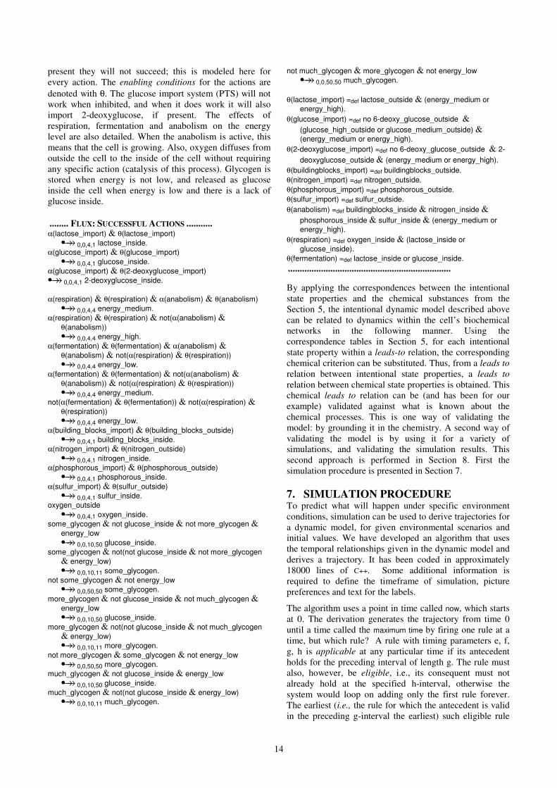
2.1 Bacterial Regulation In bacteria, as in every living cell, the regulation of internal processes invokes a multitude of processes (Neidhardt, Curtiss III, Ingraham, Lin, Brooks Low, Magasanik, Reznikoff, Riley, Schaechter & Umbarger, 1996). In Sections 2 to 4, for reasons of presentation, the regulation of the lactose import is taken as an example (cf., left-hand side of Figure 1). When lactose is added to the environment of the cell, some of it enters through the lactose permease, provided that the latter has been synthesized in the cell’s ancestors. The intracellular lactose is then isomerized to allolactose by the enzyme that also splits it into glucose and galactose (two sugars that are better fit for subsequent metabolism). Allolactose is the intracellular reporter (indicator substance) of extracellular lactose. Transcriptional, translational, and metabolic regulation then interact to modify the behaviour of the cell. The DNA associated with lactose import is the lac operon. In order to create more of lactose

permease and β-galactosidase eventually, the operon must be transcribed. This transcription only takes place when substances (called the activation proteins and repressors) are bound to, or dissociate from the DNA in order for transcription to begin, a process called transcription

regulation. The two conditions are that (i) allolactose bind to the lac-repressor and (ii) that cAMP, i.e. the substance reporting the absence of extracellular glucose, bind to the activating protein CRP. Transcription of the lac operon results in a string of mRNA encoding lactose

permease, β-galactosidase and a third protein. From this mRNA the proteins can be created in a process called translation and some subsequent processing and translocation.

For some systems there is also translational or post-

translation regulation, although not so much for the lac operon. This may involve the addition of a prosthetic group or cofactor to the enzyme. In the lactose system, there is a major additional regulation by glucose import. When glucose is taken up, the protein IIAGlc is dephosphorylated. Therewith the concentration of IIAGlc-phosphate decreases. IIAGlc-phosphate is an activator of adenylate cyclase, the enzyme that synthesizes cAMP, and this is one mechanism through which cAMP reports the absence of extracellular glucose (see above). Lactose import pathway itself is also stopped, when glucose is imported, because the unphosphorylated IIAGlc inhibits the permease. This is one example of ‘cross-talk’ between regulatory routes, i.e., glucose does not only regulate its own consumption but also that of (many) other substrates, such as lactose. In fact the repression by glucose of the consumption of other substrates is a rather general phenomenon, often called ‘glucose repression’ or ‘catabolite repression’ For two recent reviews see (Warner and Lolkema, 2003; Bruckner and Titgemeyer, 2002).

It is not quite clear why glucose repression entails two mechanisms, one involving IIAGlc-P and cAMP and the other just IIA. At high magnitudes of the transmembrane electrochemical potential difference for protons (a second form of the energy state of the cell), cAMP is extruded from the cell. Accordingly, cAMP may monitor the conditions that glucose is present and the energy status of the cell is high. IIA may monitor that much glucose is present relative to the energy state of the cell (at reduced energy levels of the cell, PTS activity is reduced [Rohwer et al., 1996], presumably because uptake requires Gibbs energy).

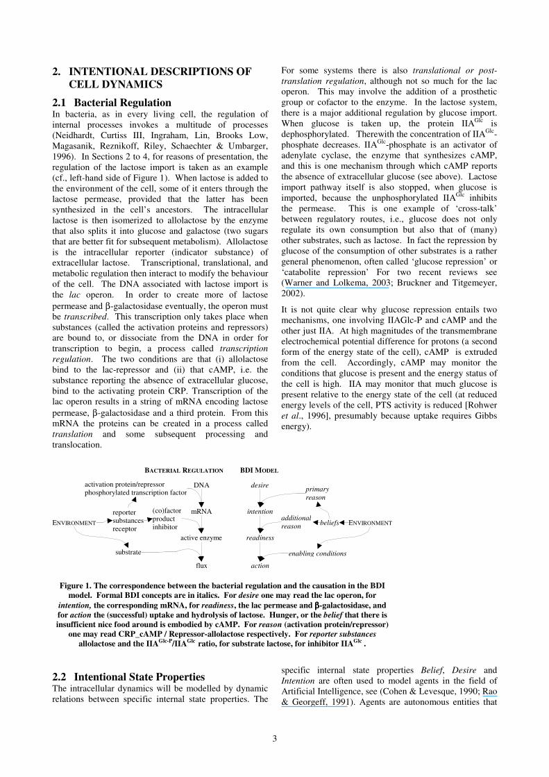
BACTERIAL REGULATION BDI MODEL

DNA

mRNA

active enzyme

flux

desire

intention

readiness

action

ENVIRONMENT ENVIRONMENT

reportersubstancesreceptor

beliefs

activation protein/repressorphosphorylated transcription factor

(co)factorproductinhibitor

substrate

primary

reason

additional

reason

enabling conditions

Figure 1. The correspondence between the bacterial regulation and the causation in the BDI

model. Formal BDI concepts are in italics. For desire one may read the lac operon, for

intention, the corresponding mRNA, for readiness, the lac permease and ββββ-galactosidase, and

for action the (successful) uptake and hydrolysis of lactose. Hunger, or the belief that there is

insufficient nice food around is embodied by cAMP. For reason (activation protein/repressor)

one may read CRP_cAMP / Repressor-allolactose respectively. For reporter substances

allolactose and the IIAGlc-P/IIAGlc ratio, for substrate lactose, for inhibitor IIAGlc .

2.2 Intentional State Properties The intracellular dynamics will be modelled by dynamic relations between specific internal state properties. The

specific internal state properties Belief, Desire and Intention are often used to model agents in the field of Artificial Intelligence, see (Cohen & Levesque, 1990; Rao & Georgeff, 1991). Agents are autonomous entities that

4

sense and act on the world. The interdependencies between the notions, in Figure 1 right hand side, are based upon a number of assumptions on beliefs, desires, and intentions. The assumptions made keep the notions relatively simple; the approach can be extended for more complex notions.

The history or make-up of the agent leads to a set of

desires by the agent, for example a desire δ. Also the history of the agent is relevant for the information obtained previously, this information is stored as a form of memory by a set of beliefs. Some of the beliefs are

reasons for the agent to pursue some action α. As action a

realizes desire δ, thus making action α happen

accomplishes δ as well, the agent derives that it intends α. Based on the observations in the past, the agent might

come to believe that is has the opportunity to do action α.

As a realizes δ, thus by doing a the agent gets the result δ,

the agent derives that it performs α.

Assumptions on beliefs. In the simplest approach, beliefs are just based on information the agent has received by observation. Beliefs are persistent by default: the agent keeps beliefs until the belief is overridden by more recent information. This entails the first assumption relevant for modelling the biological cell: if the agent has observed a world fact, then the agent creates a belief on the world fact. The second assumption is the converse: for every belief on a world fact, the agent observed this world fact.

Assumptions on intentions and desires. In the first place, when an action is performed, the agent is assumed to have had an intention to do that. Moreover, the second assumption is that an agent who has an intention to perform an action will execute the action if an opportunity in the external world (or in the cell’s own physical internal state) occurs. Thirdly, it is assumed that every intention is based on a desire. An agent can have a desire for some state of the world as well as a desire for some action to be performed. When the agent has a set of desires, it can choose to pursue some of them. A chosen desire can only lead to an intention to engage in an action if an additional reason (Dretske, 1991) is present: the third assumption is that for each intended action there is a reason and a desire as well. The fourth assumption is that if both the desire is present and the agent believes the reason to pursue the desire is present, then the intention to perform the action will be generated.

In summary, the beliefs represent what the agent deems to be true in its environment. A belief is usually present due to sensing (in the present or in the past). Desires are interpreted as what the agent wants to accomplish or fulfill. They may exist even in the absence of beliefs. Agents can have different desires that are contradictory in their fulfillment, for example desiring lots of ice cream and a slim waist, or catabolyzing glucose and making glycogen. A reason to generate an intention, given a desire, has the form of a set of beliefs. Intentions move the agent to make something happen (act). They cause action, which may remain latent. As soon as the belief in

an opportunity (for the action) occurs, the action is initiated (readiness for the action).

Depending on the actual environment (which may be different from what the agent believes), an initiated action may lead to successful action performance or may fail to be successfully performed (e.g., the action may be blocked or disturbed in its execution). Enabling

conditions are state properties of the environment that provide the ‘physical’ possibility to perform an action successfully. Actions performed successfully by the agent affect its internal or external physical environment: the (expected) action effects. The relations between the intentional state properties are depicted on the right-hand side of Figure 1.

2.3 Intentionalisation The intentional state properties used in the BDI-model to describe the behaviour can be related to the substances involved in bacterial regulation. The internal substances relating to the situation in the environment are chosen to correspond with the beliefs. Examples are the ‘reporters’ i.e. small regulatory molecules such as cAMP or allolactose, and the phoshorylation states of the histidine protein kinase domains.

When processed by the ‘thinking’ that can correspond to binding to, or phosphoryl transfer to transcription factors, that transcription factor becomes activated, i.e., a reason to generate an intention, given the presence of the desire. When such required reasons are present, the parts of the DNA (sets of genes, or operons) that correspond to a desire are activated. Within the BDI model a desire together with reasons results irrevocably in an intention.

In our model mRNA is chosen to correspond with an intention. The conditions for transcriptional regulation are the dissociation of the repressor protein and the association of the CRP protein. Therefore we consider the complex between the repressor protein and allolactose one reason and the complex between cAMP and CRP the second necessary reason for transcription of the lac operon. (More precisely, we consider uncomplexed repressor protein or uncomplexed CRP sufficient reason not to transcribe the operon.)

The enzymes created by translation are used to increase the flux of chemical reactions (which corresponds to action in the intentional model). Thus, the active enzymes are chosen to correspond with action initiation or readiness for action. Given the intention (represented by mRNA), the (co)factors necessary for the translation of mRNA into enzymes correspond with reasons for action initiation; i.e., for creating action readiness. Such reasons take the form of a set of beliefs (on properties of the environment) in an opportunity to perform the action successfully. An enzyme does not always need to be active. An inactive enzyme is not viewed as action initiation. The activity of an enzyme depends on covalent modifications or the presence of inhibitors or activators. These are also part of the reasons (beliefs in an opportunity) for action initiation. In our case no-IIAGlc is

5

a reason for lactose uptake, as IIAGlc is an inhibitor of the lac permease.

The enabling conditions for an action correspond to the physical presence of the substrates of the reaction catalysed by the enzyme. When an enzyme effects flux (i.e., actually catalyses its reaction), this corresponds to successful action performance in the world.

In Figure 1 the correspondence between the intentional state properties and the chemical regulation of the bacterium is displayed.

3. A CONTINUOUS-TIME DISCRETE-

STATE MODEL

3.1 Temporal Modelling of Continuous

Processes Our temporal modelling approach is first illustrated for continuous flows realised by chemical reactions. The transcription of the lac operon will be the leading example:

nucleotide 3-phosphates + DNA_lactose ↔ mRNA_lactose +

DNA_lactose (1)

Formulae like (1) do not express inhibitors, activators, speed and equilibrium conditions. For example lactose and CRP_cAMP are the activation proteins regulating the transcription of the lac operon :

Regulators: Repressor_allolactose 0.01 mM, CRP_cAMP 0.01 mM,

kcat=0.01 s-1, Keq=∞ (2)

Here the Keq value of infinity refers to the irreversibility of the process, the kcat value is an estimation. What does this reaction do over time? Given sufficient lactose, CRP_cAMP and nucleotide tri phosphates (NTP’s), the mRNA_lactose will start to be produced, and after a certain delay a significant amount of mRNA_lactose will be present. The concentrations of repressor_allolactose and CRP_cAMP need to be sufficiently high for a certain period of time in order for the reaction to proceed, a concentration of at least 0.01 mM (the threshold) suffices in the example. The amount of NTP’s needed for the reaction to proceed is at least 0.1 mM, but a steady excess of nucleotides will be assumed. In order for the reaction to occur, the amount of mRNA must not be so high as to impede the reaction, a concentration lower than about to 0.01 mM in this example. The reaction proceeds and eventually a steady state can be reached where the mRNA degrades equally rapidly following some first order process.

We now define temporal relationships between the sources and the effect as follows:

DNA_lactose & No-free-Repressor & CRP_cAMP •→→e,f,g,h

mRNA_lactose (3)

On the left-hand side the conditions are listed. Since NTP’s are always in excess, they are not mentioned. The DNA_lactose refers to the presence of the lactose-operon in the DNA. No-free-Repressor refers to the required

presence of allolactose that binds the repressor protein. CRP_cAMP indicates the requirement for (i.e., concentration above a threshold value of) CRP_cAMP to bind to the activation sites of the operon. On the right-hand side, the change is listed, mRNA_lactose meaning the production of ‘sufficient’ lactose mRNA. It should be noted that in our method concentrations will not be on a continuous scale, but substances will be either present at sufficient quantity or absent. If needed, the method allows to distinguish more discrete categories.

The parameters e, f, g and h are explained as follows. Before the rule has effect, the antecedent (the part before the arrow) needs to occur a certain minimum duration g, as it would not be realistic to expect that if the antecedent is there for a very short time, that the consequent (the part after the arrow) is already generated. If the consequent indeed is generated, the rule garantees it will be there for at least a certain duration h. The parameters e and f specify the minimum and maximum delay in the process: how long after the occurrence interval of the antecedent the consequent will start to occur. These are bounds between which a random delay can be used. However, in many cases the delay is made deterministic (by taking the midpoint of the interval from e to f). Realistic parameters for the values of e, f, g and h for the example are e = 60 s, f = 60 s, g = 1 s and h = 40 s, as the process to create the mRNA takes about 60 seconds, and the mRNA will stay in existence for about 40 seconds on average. When the antecedent holds for 1 second or more, the transcription process starts. In the next section the temporal relationship used here is explained in more mathematical detail.

3.2 States, trajectories, and ‘Leads To’

Relations In the previous section a temporal model has been presented of a chemical process using categories of substance concentrations and temporal relationships between these. This section defines more precisely the

temporal relation •→→ within the LEADSTO language (Jonker, Treur and Wijngaards, 2003; Bosse, Jonker, Meij,

and Treur, 2007) that is used as a vehicle to formally specify the temporal relations of the developed BDI-model. This relation is defined in terms of its semantics. In order to understand the definition, a few semantic concepts must be understood.

State and Trajectory The trajectory of a system at a certain time point is described by a mapping that assigns a truth-value (true, or false) to all state atoms, i.e., all atomic (elementary descriptive) properties or statements relevant for a state of that system. A trajectory of a system is a specific sequence of states of the system over a continuous time

frame T (chosen to be the real numbers). The set W is the

set of all possible trajectories. Let T be a trajectory, and t a

time point, then state(T, t) denotes the state of the system

in trajectory T at time point t. Let α be a state property

(i.e., a proposition in atomic state properties), then state(T,

6

t) |== α is used to denote that in a given trajectory T at time

t the state property α holds.

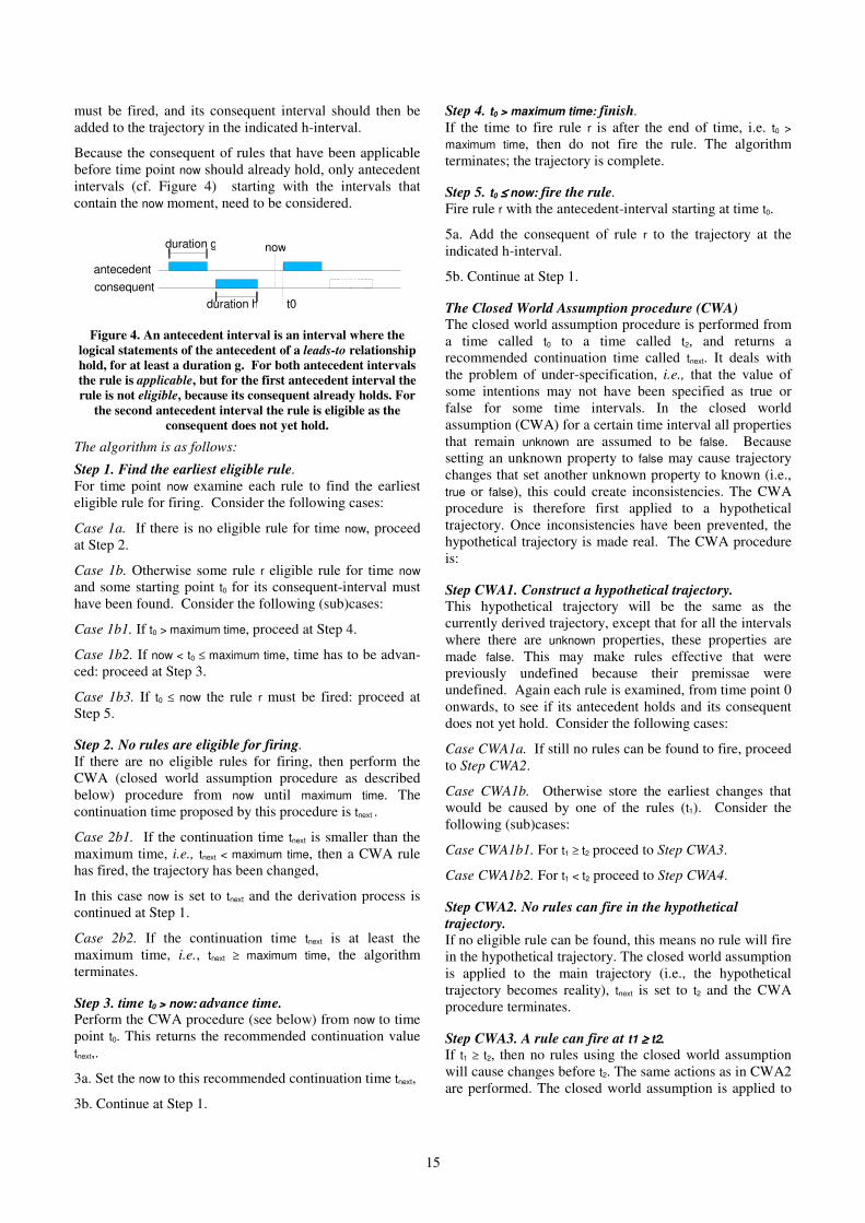
The formal definition of the temporal operator •→→ is expressed in two parts, the forward-in-time part and the backward-in-time part. Time intervals are denoted by [x, y) (from and including x, to but not including y) and [x, y] (the same, but including the y value).

Definition (The relationship ••••→→→→→→→→)

Let α and β be state properties, and W the set of all

possible trajectories. Then α follows β, as denoted by α

→→e, f, g, h β, with time delay interval [e, f] and duration parameters g and h if

∀T ∈ W ∀t1:

[∀t ∈ [t1 - g, t1) : state(T, t) |== α ⇒

∃d ∈ [e, f] ∀t ∈ [t1 + d, t1 + d + h) :

state(T, t) |== β ]

This makes α a sufficient condition for β. Conversely,

the state property β originates in state property α, as denoted by

α •e, f, g, h β, with time delay [e, f] and duration parameters g and h, if

∀ T ∈ W ∀ t2:

[∀t ∈ [t2, t2 + h) : state(T, t) |== β ⇒

∃d ∈ [e, f] ∀t ∈ [t2 - d - g, t2 - d)

state(T, t) |== α]

This makes α a necessary condition for β. If both α →→

e,f,g,h β, and α •e,f,g,h β hold, α is a necessary and

sufficient pre-condition for β, α leads to β, as denoted by:

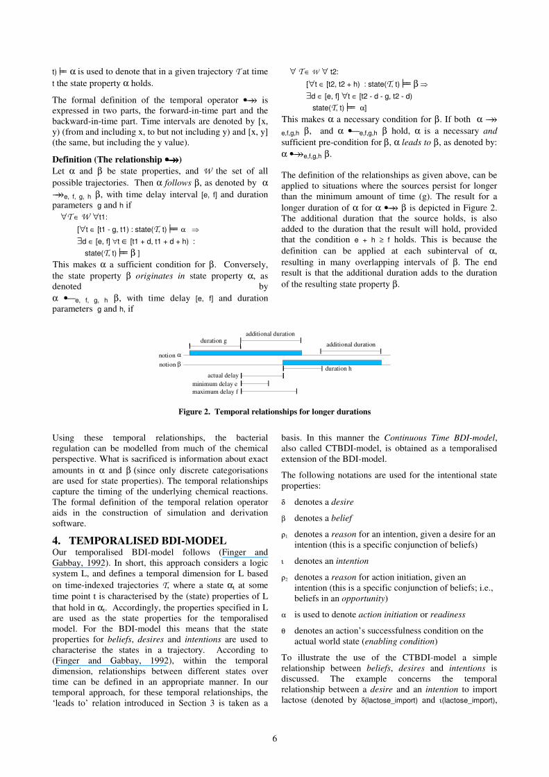
α •→→e,f,g,h β. The definition of the relationships as given above, can be applied to situations where the sources persist for longer than the minimum amount of time (g). The result for a

longer duration of α for α •→→ β is depicted in Figure 2. The additional duration that the source holds, is also added to the duration that the result will hold, provided that the condition e + h ≥ f holds. This is because the

definition can be applied at each subinterval of α,

resulting in many overlapping intervals of β. The end result is that the additional duration adds to the duration

of the resulting state property β.

notion α notion β

actual delay

duration g

duration h

minimum delay e maximum delay f

additional duration additional duration

Figure 2. Temporal relationships for longer durations

Using these temporal relationships, the bacterial regulation can be modelled from much of the chemical perspective. What is sacrificed is information about exact

amounts in α and β (since only discrete categorisations are used for state properties). The temporal relationships capture the timing of the underlying chemical reactions. The formal definition of the temporal relation operator aids in the construction of simulation and derivation software.

4. TEMPORALISED BDI-MODEL Our temporalised BDI-model follows (Finger and Gabbay, 1992). In short, this approach considers a logic system L, and defines a temporal dimension for L based

on time-indexed trajectories T, where a state αt at some

time point t is characterised by the (state) properties of L

that hold in αt. Accordingly, the properties specified in L are used as the state properties for the temporalised model. For the BDI-model this means that the state properties for beliefs, desires and intentions are used to characterise the states in a trajectory. According to (Finger and Gabbay, 1992), within the temporal dimension, relationships between different states over time can be defined in an appropriate manner. In our temporal approach, for these temporal relationships, the ‘leads to’ relation introduced in Section 3 is taken as a

basis. In this manner the Continuous Time BDI-model, also called CTBDI-model, is obtained as a temporalised extension of the BDI-model.

The following notations are used for the intentional state properties:

δ denotes a desire

β denotes a belief

ρ1 denotes a reason for an intention, given a desire for an intention (this is a specific conjunction of beliefs)

ι denotes an intention

ρ2 denotes a reason for action initiation, given an intention (this is a specific conjunction of beliefs; i.e., beliefs in an opportunity)

α is used to denote action initiation or readiness

θ denotes an action’s successfulness condition on the actual world state (enabling condition)

To illustrate the use of the CTBDI-model a simple relationship between beliefs, desires and intentions is discussed. The example concerns the temporal relationship between a desire and an intention to import lactose (denoted by δ(lactose_import) and ι(lactose_import),

7

respectively) vis-à-vis the reason (denoted by ρ1(lactose_import)) to generate the intention. In chemical terms the example concerns the possibility of de-repressing the operon and binding RNA polymerase to the promotor. The desire and the reason for the intention, given the desire, should persist for at least some duration. After a time period larger than the minimum delay and shorter than the maximum delay, the intention starts to hold for some other duration. This temporal relationship is denoted in LEADSTO format as follows:

δ(lactose_import)

& ρ1(lactose_import)

•→→e,f,g,h ι(lactose_import). (4a)

Here g and h are parameters for durations and e and f are delay parameters. See also temporal relation (3) in Section 3.1. Here the reason ρ1(lactose_import) relates to a conjunction of two internal chemical state properties:

• the allalactose concentration is above 0.1 mM (assuming this entails the presence of the allolactose-repressor complex), and

• the cAMP concentration is above 0.01 mM (assuming this entails the presence of the CRP_cAMP complex).

This conjunction of internal chemical state properties is interpreted as a conjunction of beliefs; therefore, by definition (indicated by the subscript def):

ρ1(lactose_import) =def

β(lactose_outside) & β(famine).

where famine means that only a low concentration of glucose is present in the environment (see also Section 5). The first belief corresponds to the internal chemical state property that the allalactose concentration is above 0.1 mM, the second belief corresponds to the property that the cAMP concentration is above 0.01 mM.

So, temporal relation (4a) can be written alternatively as:

δ(lactose_import)

& β(lactose_outside)

& β(famine)

•→→e,f,g,h ι(lactose_import). (4b)

This temporal relation was inspired by (Dretske, 1988), p. 112-113, where it is discussed how a behaviour M can be ‘caused by’ a combination of a desire D and a belief B representing an additional reason for the behaviour.

The intentional state properties are related to the substances, as discussed in the Sections 2 and 4.

In summary, in relation to (4a,b) the DNA relates to a desire and the mRNA to an intention. The presence of a relevant amount of allolactose (assumed equivalent to the presence of the allolactose-repressor complex) and the presence of a relevant amount of cAMP (assumed equivalent to the presence of the CRP_cAMP complex) are interpreted as the reason for the lactose import intention, given the desire. As within the BDI-model such a reason takes the form of a combination of beliefs, each

of the two internal state properties is interpreted as a belief. The NTPs and other, intermediate, substances are not labelled with intentional state properties. These substances are only the more detailed machinery of the realisation of the bacterial cognition, and are here assumed to play no decisive role in the lactose uptake behavior. It is also necessary to know which concentration of the substance is a relevant amount for the corresponding intentional state property to hold. A threshold is used to determine whether the intentional state property holds or not (discretisation of internal state properties).

Now for the timing relationships, the reaction will start to produce significant amounts of product mRNA when the regulators and sources are present in sufficiently high concentrations. Thus, it can be said that the reaction starts producing when the substances are above their threshold. All values are given in Table 1.1 Therefore, the corresponding intentional state properties will hold. Once the reaction is started, enough intermediate products in the reaction chain have to build up for the result of the process to become available.

When the result becomes available, the mRNA level will rise to a higher concentration. For the corresponding intention to hold, this concentration must be above the threshold. To get the concentration above the threshold, the rise in concentration must happen for some time. This duration, is linked to the duration that the regulators and sources were above their thresholds, giving the strength of the pulse of substances through the reaction chain. The intentional state properties corresponding to the regulators and sources must hold for at least some time, for an effect to happen.

After the effect becomes apparent, the effect will last for a period of time. The mRNA produced will stay in the cell for a while, but after some time, due to dilution or hydrolysis, the mRNA will disappear. The concentration of mRNA lowers after some time. At some point it falls below the threshold, at which time the corresponding intention no longer holds. The intentional state properties corresponding to the result thus hold for some duration after the effect starts to become apparent. The timing parameters e, f, g, and h are the same as those found in the abstract chemical model (3) in Section 3.1, thus relation (5) holds.

δ(lactose_import)

& β(lactose_outside)

& β(famine)

•→→ 60,60,1,40 ι(lactose_import). (5)

This means that if the whole antecedent

δ(lactose_import) & β(lactose_outside) &

β(famine)

1 In case parameter values were not available, we used estimated values; we refer to (Jonker et al., 2002) for estimation of these values.

8

holds for at least 1 time unit, then after 60 time units the consequent

ι(lactose_import).

will occur for at least 40 time units. In Figure 3 the timing relationships between the arguments is explained; note

that here δ is indicated by the word desire, β by belief and

ι by intention. When the source state properties are present for a duration g, then after a delay (between the minimum (e) and maximum (f) delay) the resulting state properties are present for duration h. For each intentional state property, its status over time is depicted. Time increases towards the right. The shaded boxes indicate when the state properties hold.

desire(lactose_import)

intention(lactose_import)

belief(lactose_outside) belief(no glucose_outside)

actual delay

duration g

duration h minimum delay maximum delay

time holds notion

Figure 3. Explanation of timings for temporal relationships. The lighter colour refers to minimally required duration, the

darker colour to spurious duration

5. RELATIONS BETWEEN

INTENTIONAL AND CHEMICAL

STATE PROPERTIES: AN EXAMPLE In this section an extended example is described, which covers the import of nutrition, catabolism and anabolism. It is an extension of the complex steady-state example of the bacterium Escherichia coli presented in (Jonker et al., 2002), to (dynamically) varying environments:

− Lactose can be present or absent.

− Glucose can be present in low, medium or high quantities.

− Nitrogen can be present or absent.

− Phosphorous can be present or absent.

− Sulfur can be present or absent.

− Carbon building blocks can be present or absent.

− Molecular Oxygen can be present or absent.

− 2-deoxyglucose can be present or absent.

− 6-deoxyglucose can be present or absent.

Glucose is modeled in slightly more detail than is lactose, by distinguishing three states for external glucose rather than two. The inhibitor 2-deoxyglucose looks like glucose to the cell and is taken up but cannot be processed internally, whilst 6-deoxyglucose blinds the cell to the presence of glucose or 2-deoxyglucose, as it competes for the glucose uptake system. The Gibbs energy level of the cell is also evaluated in three gradations, i.e. low, medium or high.

The terms used to define the model are given in Table 1. As compared to that in (Jonker et al., 2002), the denotation has been adjusted for readability. The chemical

criteria and the corresponding logical notation for the intentional state properties are both given, again improved with respect to those in (Jonker et al., 2002). The correspondence between the chemical and the intentional terms is shown in Figure 1.

Average dissociation constants of enzymes for their substrates and products are in the order of mM concentrations (estimated average Km of about 0.1 mM; http://www.brenda-enzymes.info/). We have therefore chosen for most of the molecules, 0.1 mM as the concentration below which they are thought to be absent and above which they are sensed as present. Of course this is a gross over-simplification but it should be realized that with the simulations we aim at illustrating some of the BDI-modelling concepts and that the specific parameter values are not crucial for the simulation results. For some of the molecules we have chosen different values for the lower concentration of sensing, i.e. glucose at 0.01 mM (Km of PTS uptake system for glucose is 0.01 mM; Stock et al., 1982). Translation of ATP/ADP ratios to the energy status of the cell: ATP/ADP < 0.5, little Gibs free energy present; 0.5 < ATP/ADP < 5, some Gibbs free energy available; ATP/ADP > 5, much Gibbs free energy available were chosen on the basis of experimental ATP/ADP measurements in E. coli (Van Workum et al., 1996). Threshold levels of cAMP concentrations during feast or famine were estimated from (Death and Ferenci, 1994). Concentrations of mRNA and protein are estimates.

actual delay

mimimum delay e

maximum delay f

9

Table 1. The chemical criteria and intentional state properties: state properties.

DW= dry weight, mM=mmol/liter.

State Properties Chemical Criterion Logical Notation

In the external world there is almost

no glucose present.

outside glucose concentration is below

0.01 mM

glucose_low_outside

In the external world some glucose is

present.

outside glucose concentration between

0.01 and 0.1 mM

glucose_medium_outside

In the external world a lot of glucose

is present.

outside glucose concentration exceeds

0.1 mM

glucose_high_outside

In the external world lactose is

present.

outside lactose concentration exceeds

0.1 mM

lactose_outside

In the external world 2-deoxyglucose

is present.

outside 2-deoxyglucose concentration

exceeds 0.1 mM

2-deoxyglucose_outside

In the external world 6-deoxyglucose

is present.

outside 6-deoxyglucose concentration

exceeds 0.1 mM

6-deoxyglucose_outside

In the external world oxygen is

present.

outside oxygen concentration exceeds

0.1 mM

oxygen_outside

Building blocks are present outside

the cell.

The building blocks’ concentration

outside the cell exceeds 0.1 mM

building_blocks_outside

Nitrogen is present outside the cell. outside ammonia concentration exceeds

0.1 mM

nitrogen_outside

Phosphorous is present outside the

cell.

outside phosphate concentration exceeds

0.1 mM

phosphorous_outside

Sulfur is present outside the cell. outside sulfate concentration exceeds

0.1 mM

sulfur_outside

Catabole nutrition is readily available

outside the cell

uninhibited glucose high/medium

present

feast

No catabole nutrition is readily

available outside the cell

no uninhibited glucose high/medium

present

famine

Inside the cell glucose is present. glucose-6-phosphate concentration

inside exceeds 0.1 mM

glucose_inside

Inside the cell lactose is present. lactose concentration inside exceeds 0.1

mM

lactose_inside

Inside the cell 2-deoxyglucose is

present.

2-deoxyglucose-6-phosphate

concentration inside exceeds 0.1 mM

2-deoxyglucose_inside

Inside the cell oxygen is present. dissolved oxygen concentration inside

the cell exceeds 0.1 mM

oxygen_inside

Building blocks are present inside the

cell.

The building blocks’ concentration

inside the cell exceeds 0.1 mM

building_blocks_inside

Nitrogen is present inside the cell. ammonia concentration inside the cell

exceeds 0.1 mM

nitrogen_inside

Phosphorous is present inside the cell. phosphate concentration inside the cell

exceeds 0.1 mM

phosphorous_inside

Sulfur is present inside the cell. sulfate concentration inside the cell

exceeds 0.1 mM

sulfur_inside

Some glycogen is present C6 units per cell exceed 10000 some_glycogen

More glycogen is present C6 units per cell exceed 2 million more_glycogen

Much glycogen is present C6 units per cell exceed 25 million much_glycogen

Little Gibbs energy is available inside

the cell.

ATP/ADP ratio below 0.5 energy_low

Some Gibbs energy is available

inside the cell.

ATP/ADP between 0.5 and 5 energy_medium

Much Gibbs energy is available

inside the cell.

ATP/ADP ratio exceeds 5 energy_high

Table 2. The chemical criteria and intentional state properties: Beliefs.

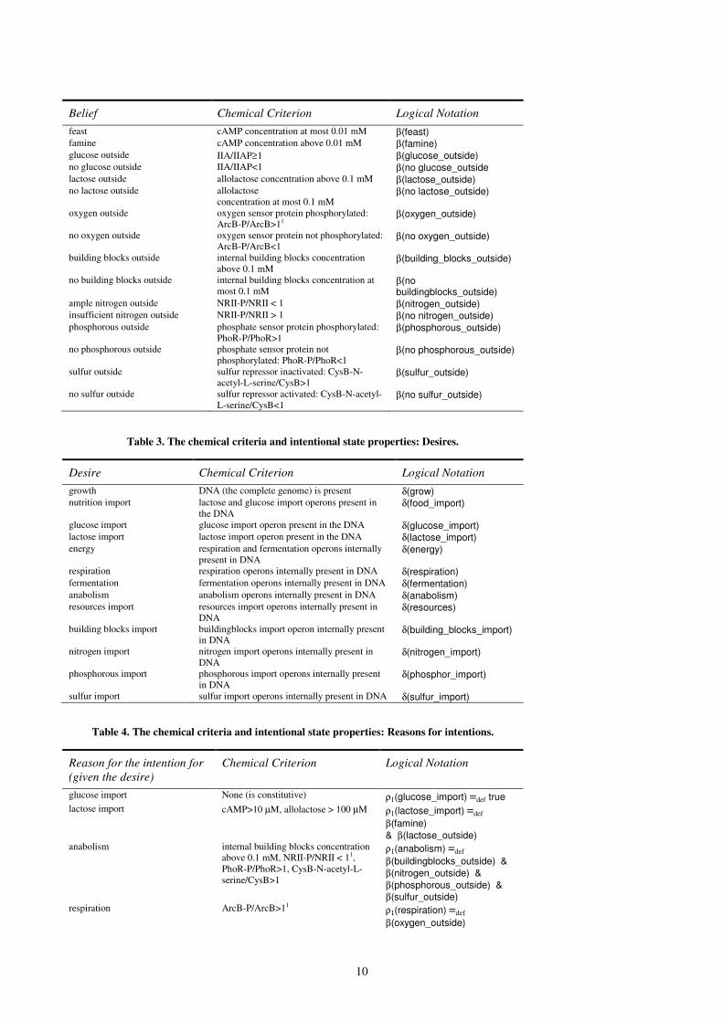
10

Belief Chemical Criterion Logical Notation

feast cAMP concentration at most 0.01 mM β(feast) famine cAMP concentration above 0.01 mM β(famine) glucose outside IIA/IIAP≥1 β(glucose_outside) no glucose outside IIA/IIAP<1 β(no glucose_outside lactose outside allolactose concentration above 0.1 mM β(lactose_outside) no lactose outside allolactose

concentration at most 0.1 mM β(no lactose_outside)

oxygen outside oxygen sensor protein phosphorylated: ArcB-P/ArcB>11

β(oxygen_outside)

no oxygen outside oxygen sensor protein not phosphorylated: ArcB-P/ArcB<1

β(no oxygen_outside)

building blocks outside internal building blocks concentration above 0.1 mM

β(building_blocks_outside)

no building blocks outside internal building blocks concentration at most 0.1 mM

β(no buildingblocks_outside)

ample nitrogen outside NRII-P/NRII < 1 β(nitrogen_outside) insufficient nitrogen outside NRII-P/NRII > 1 β(no nitrogen_outside) phosphorous outside phosphate sensor protein phosphorylated:

PhoR-P/PhoR>1 β(phosphorous_outside)

no phosphorous outside phosphate sensor protein not phosphorylated: PhoR-P/PhoR<1

β(no phosphorous_outside)

sulfur outside sulfur repressor inactivated: CysB-N-acetyl-L-serine/CysB>1

β(sulfur_outside)

no sulfur outside sulfur repressor activated: CysB-N-acetyl-L-serine/CysB<1

β(no sulfur_outside)

Table 3. The chemical criteria and intentional state properties: Desires.

Desire Chemical Criterion Logical Notation

growth DNA (the complete genome) is present δ(grow) nutrition import lactose and glucose import operons present in

the DNA δ(food_import)

glucose import glucose import operon present in the DNA δ(glucose_import) lactose import lactose import operon present in the DNA δ(lactose_import) energy respiration and fermentation operons internally

present in DNA δ(energy)

respiration respiration operons internally present in DNA δ(respiration) fermentation fermentation operons internally present in DNA δ(fermentation) anabolism anabolism operons internally present in DNA δ(anabolism) resources import resources import operons internally present in

DNA δ(resources)

building blocks import buildingblocks import operon internally present in DNA

δ(building_blocks_import)

nitrogen import nitrogen import operons internally present in DNA

δ(nitrogen_import)

phosphorous import phosphorous import operons internally present in DNA

δ(phosphor_import)

sulfur import sulfur import operons internally present in DNA δ(sulfur_import)

Table 4. The chemical criteria and intentional state properties: Reasons for intentions.

Reason for the intention for

(given the desire)

Chemical Criterion Logical Notation

glucose import None (is constitutive) ρ1(glucose_import) =def true

lactose import cAMP>10 µM, allolactose > 100 µM ρ1(lactose_import) =def β(famine)

& β(lactose_outside) anabolism internal building blocks concentration

above 0.1 mM, NRII-P/NRII < 11, PhoR-P/PhoR>1, CysB-N-acetyl-L-serine/CysB>1

ρ1(anabolism) =def β(buildingblocks_outside) &

β(nitrogen_outside) &

β(phosphorous_outside) &

β(sulfur_outside) respiration ArcB-P/ArcB>11 ρ1(respiration) =def

β(oxygen_outside)

11

fermentation ArcB-P/ArcB<1 ρ1(fermentation) =def β(no oxygen_outside)

building blocks import internal buildingblocks concentration above 0.1 mM

ρ1(buildingblocks_import) =def β(buildingblocks_outside)

nitrogen import NRII-P/NRII < 1 ρ1(nitrogen_import) =def β(nitrogen_outside)

phosphorous import PhoR-P/PhoR>1 ρ1(phosphorous_import) =def β(phosphorous_outside)

sulphur import CysB-N-acetyl-L-serine/CysB>1 ρ1(sulphur_import) =def β(sulphur_outside)

Table 5. The chemical criteria and intentional state properties: Intentions.

Intention for Chemical Criterion Logical Notation

glucose import glucose-import (PTS) mRNA-concentration above

1 µM ι(glucose_import)

lactose import lac-mRNA concentration above 1 µM ι(lactose_import) anabolism anabolism-mRNA concentration above 1 µM ι(anabolism) respiration respiration-mRNA concentration above 1 µM ι(respiration) fermentation fermentation-mRNA concentration above 1 µM ι(fermentation) building blocks import building-blocks import mRNA-concentration

above 1 µM ι(buildingblocks_import)

nitrogen import nitrogen-import mRNA concentration above 1

µM ι(nitrogen_import)

phosphorous import phosphate-import mRNA concentration 1 µM ι(phosphorous_import) sulfur import sulfur-import mRNA concentration above 1 µM ι(sulfur_import)

Table 6. The chemical criteria and intentional state properties: Reasons for Action Initiation.

Reason for action

initiation or readiness for

(given the intention)

Chemical Criterion Logical Notation

glucose import cAMP concentration at most 0.01 mM ρ2(glucose_import) =def β(feast)

lactose import allolactose concentration above 0.1 mM and IIA/IIAP<1

ρ2(lactose_import) =def β(lactose_outside) & β(no

glucose_outside) anabolism ATP/ADP ratio exceeds 0.5 ρ2(anabolism) =def

β(energy_medium or energy_high)

respiration None ρ2(respiration) =def true

fermentation None ρ2(fermentation) =def true

building blocks import None ρ2(buildingblocks_import) =def true

nitrogen import None ρ2(nitrogen_import) =def true

phosphorous import None ρ2(phosphorous_import) =def true

sulphur import None ρ2(sulphur_import) =def true

Table 7. The chemical criteria and intentional state properties: Readiness for Action.

Readiness for Chemical Criterion Logical Notation

glucose import glucose-import enzymes (PTS) concentration

above 10 µM α(glucose_import)

lactose import lactose-permease concentration above 10

µg/gDW α(lactose_import)

anabolism anabolic enzymes concentration above 10 µM α(anabolism) respiration respiratory chain concentration above 10

µg/gDW α(respiration)

fermentation fermentation-enzymes concentration above 10

µM α(fermentation)

building blocks import building-blocks carriers concentration above 10

µg/gDW α(building_blocks_import)

12

nitrogen import ammonium-carrier concentration above 10

µg/gDW α(nitrogen_import)

phosphor import phosphate-carrier (Pst and Pit) concentration

above 10 µg/gDW α(phosphor_import)

sulfur import sulfate carrier concentration above 10 µg/gDW α(sulfur_import)

6. THE DYNAMIC MODEL The regulation and control that govern the cellular processes will now be specified for the CTBDI-model introduced in Section 4. The temporal relationships between intentional state properties provide an abstract description of the internal dynamics that occur in E. coli. Save some oversimplifications we made here for the purpose of clarity, the resulting model should be a correct and more transparent, higher level description of the regulation process. It should be more understandable for the reader not versed in the technicalities of the chemical pathways in the cell.

The observation of the state of the outside world determines the beliefs of the bacterium. When the lactose is detected, which requires the presence and action of

lactose permease and β-galactosidase, this constitutes the belief that lactose is present. The belief that lactose is present in the environment of the cell, is denoted by β(lactose_outside). The belief that lactose is absent is denoted by β(no lactose_outside). If the cell does not obtain any information on whether lactose is outside, this is denoted by not β(lactose_outside) & not β(no lactose_outside). Notice the difference expressed by the different positions

of the negation here: not β(…) means that it is unknown to

the cell whether … holds, whereas β(no …) means that it is known that … does not hold.

The observation of glucose is complicated by possible inhibitors and influenced by the Gibbs energy status of the cell. When glucose or 2-deoxyglucose is present, and no 6-deoxyglucose is present, the cell detects glucose. Depending on the Gibbs-energy status of the cell, the amount of glucose needed to pass detection changes. When its energy level is medium or high, only a high amount of glucose is detected. When the energy level is low, also a medium amount of glucose is detectable.

These and other statements are written in a more precise form below. For instance,

lactose_outside & not β(glucose_outside)

•→→ 0,0,0.230,0.230 β(lactose_outside) & not β(no lactose_outside)

means that once is present outside the cell lactose (and no belief on glucose is there) for more than 230 milliseconds, immediately the cell believes that lactose is present (and the same for the belief about glucose) and this belief lasts for the same period of time. Here it is assumed that the synthesis of sufficient allolactose to materialize the belief takes 230 milliseconds, and that allolactose has a lifetime of 230 milliseconds. In fact, for all beliefs all delays are set to zero, and the time required for the signal to last is set to 230 milliseconds as is the lifetime of the belief. This is a gross oversimplification, but at present insufficient information exists to be much more precise, and we do not wish to enter into precise discussion of these values in this

paper. In this sense the model should be seen as an illustration only. If more precise and reliable estimations are available, it will be worthwhile to make the model more precise in a separate study.

For each of the positive statements concerning the generation of the beliefs, we also apply the corresponding negative statement. For instance for:

sulfur_outside

•→→ 0,0,0.230,0.230 β(sulfur_outside) &

not β(no sulfur_outside).

we apply:

no sulfur_outside

•→→ 0,0,0.230,0.230 β(no sulfur_outside) &

not β(sulfur_outside).

This is a bit superfluous, as the use of the •→→ symbol implies a both necessary and sufficient condition. Moreover, the finite lifetime of the belief has the effect that in the absence of the external condition the belief disappears. Our way of also having the negative statement does have some detailed temporal effects and is a bit more general. The negative statements are not shown below as they can easily be derived from the positive statements.

..... REPORTER MOLECULES: BELIEFS ........ lactose_outside & β( no glucose_outside)

•→→ 0,0,0.230,0.230 β(lactose_outside) &

not β(no lactose_outside).

no 6-deoxyglucose_outside & ( glucose_medium_outside or

glucose_high_outside or (glucose_low_outside & energy_high)

or 2-deoxyglucose_outside)

•→→ 0,0,0.230,0.230 β(feast) & not β(famine).

6-deoxyglucose_outside & energy_high

•→→ 0,0,0.230,0.230 β(feast) & not β(famine).

(glucose_high_outside or 2-deoxyglucose_outside) &

no 6-deoxyglucose_outside & (energy_high or

energy_medium)

•→→ 0,0,0.230,0.230 β(glucose_outside) &

not β(no glucose_outside).

(glucose_medium_outside or glucose_high_outside or

2-deoxyglucose_outside) &

no 6-deoxyglucose_outside & energy_low

•→→ 0,0,0.230,0.230 β(glucose_outside) and

not β(no glucose_outside).

oxygen_outside

•→→ 0,0,0.230,0.230 β(oxygen_outside) &

not β(no oxygen_outside).

building_blocks_outside

•→→ 0,0,0.230,0.230 β(buildingblocks_outside) &

not β(no buildingblocks_outside).

nitrogen_outside

•→→ 0,0,0.230,0.230 β(nitrogen_outside) &

not β(no nitrogen_outside).

phosphorous_outside

•→→ 0,0,0.230,0.230 β(phosphorous_outside) &

not β(no phosphorous_outside).

sulfur_outside

•→→ 0,0,0.230,0.230 β(sulfur_outside) &

not β(no sulfur_outside).

13

.....................................................................

The desires of the cell are realised by its genome. For the time span of the chosen example, the genome of the cell does not change. Therefore, the desires always hold. The overall desire is taken to be the desire to grow, representing the entire genome. For this desire the cell desires Gibbs energy, anabolism and food import. For the energy desire the cell desires respiration or fermentation. For the anabolism desire the cell desires resources, for which it desires to import building blocks, nitrogen, phosphorous and sulfur. For the food import desire the cell desires to import lactose and glucose.

................... GENES: DESIRES ...................... δ(grow).

δ(energy).

δ(respiration).

δ(fermentation).

δ(anabolism).

δ(resources).

δ(building_blocks_import).

δ(nitrogen_import).

δ(phosphorous_import).

δ(sulfur_import).

δ(food_import).

δ(lactose_import).

δ(glucose_import).

.....................................................................

The intentions to prepare for actions follow the presence of a desire and a corresponding reason. In some cases the reason is absent, denoted as ‘true’. Then it always holds; it is constitutive in microbiological terms. The intention for the import of lactose requires a more specific reason; lactose must be believed externally present and glucose must be believed externally absent, and this must have materialized in the presence of CRP_cAMP and lac repressor-allolactose complexes (in this paper we consider this materialization to be immediate). For the intention for respiring and fermenting, the corresponding reason involves a belief in the external presence or absence respectively, of molecular oxygen. given a desire, the reason for creating the intention for importing a resource, is that this resource must be believed to be present outside the cell. The intention for anabolism requires all necessary resources to be believed present.

............... MRNAS: INTENTIONS .................. δ(lactose_import) & ρ1(lactose_import)

•→→ 60,60,1,40 ι(lactose_import). δ(glucose_import) & ρ1(glucose_import)

•→→ 60,60,1,40 ι(glucose_import). δ(respiration) & ρ1(respiration)

•→→ 60,60,1,40 ι(respiration). δ(fermentation) & ρ1(fermentation)

•→→ 60,60,1,40 ι(fermentation). δ(anabolism) & ρ1(anabolism)

•→→ 60,60,1,40 ι(anabolism). δ(buildingblocks_import) & ρ1(buildingblocks_import)

•→→ 60,60,1,40 ι(buildingblocks_import). δ(nitrogen_import) & ρ1(nitrogen_import)

•→→ 60,60,1,40 ι(nitrogen_import). δ(phosphorous_import) & ρ1(phosphorous_import)

•→→ 60,60,1,40 ι(phosphorous_import).

δ(sulphur_import) & ρ1(sulphur_import)

•→→ 60,60,1,40 ι(sulphur_import).

ρ1(lactose_import) =def β(lactose_outside)

& β(famine).

ρ1(glucose_import) =def true.

ρ1(respiration) =def β(oxygen_outside).

ρ1(fermentation) =def β(no oxygen_outside).

ρ1(anabolism) =def β(building_blocks_outside)

& β(nitrogen_outside)

& β(phosphorous_outside)

& β(sulfur_outside).

ρ1(buildingblocks_import) =def β(building_blocks_outside).

ρ1(nitrogen_import) =def β(nitrogen_outside).

ρ1(phosphorous_import) =def β(phosphorous_outside).

ρ1(sulphur_import) =def β(sulfur_outside).

.....................................................................

The action initiation or readiness to perform an action follow the presence of the intention for them and a suitable (additional) reason. Many are denoted as ‘true’, thus no regulation happens for them at this stage. Given the intention, the readiness for lactose import requires the reason that lactose is believed externally present and glucose is believed externally absent. This reflects the inhibitory effect of IIAGlc on lactose permease. The readiness for glucose import also requires a reason (in addition to the presence of the intention), i.e., that glucose is believed present externally.

.. ENZYMES: INITIATION OR READINESS .... ι(lactose_import) & ρ2(lactose_import)

•→→ 0,0,60,600 α(lactose_import).

ι(glucose_import) & ρ2(glucose_import) •→→ 0,0,60,600 α(glucose_import).

ι(respiration) & ρ2(respiration) •→→ 0,0,60,600 α(respiration).

ι(fermentation) & ρ2(fermentation) •→→ 0,0,60,600 α(fermentation).

ι(anabolism) & ρ2(anabolism) •→→ 0,0,60,600 α(anabolism).

ι(building_blocks_import) & ρ2(buildingblocks_import) •→→ 0,0,60,600 α(buildingblocks_import).

ι(nitrogen_import) & ρ2(nitrogen_import) •→→ 0,0,60,600 α(nitrogen_import).

ι(phosphorous_import) & ρ2(phosphorous_import) •→→ 0,0,60,600 α(phosphorous_import).

ι(sulphur_import) & ρ2(sulphur_import) •→→ 0,0,60,600 α(sulphur_import).

ρ2(lactose_import) =def β(lactose_outside)

& β(no glucose_outside).

ρ2(glucose_import) =def β(feast).

ρ2(respiration) =def true.

ρ2(fermentation) =def true.

ρ2(anabolism) =def

β(energy_medium or energy_high).

ρ2(buildingblocks_import) =def true.

ρ2(nitrogen_import) =def true.

ρ2(phosphorous_import) =def true.

ρ2(sulphur_import) =def true.

.....................................................................

These actions, i.e., the effects of action initiation or readiness are modelled as well. Even though the cell may catalyse particular processes, if their sources are not

14

present they will not succeed; this is modeled here for every action. The enabling conditions for the actions are

denoted with θ. The glucose import system (PTS) will not work when inhibited, and when it does work it will also import 2-deoxyglucose, if present. The effects of respiration, fermentation and anabolism on the energy level are also detailed. When the anabolism is active, this means that the cell is growing. Also, oxygen diffuses from outside the cell to the inside of the cell without requiring any specific action (catalysis of this process). Glycogen is stored when energy is not low, and released as glucose inside the cell when energy is low and there is a lack of glucose inside.

........ FLUX: SUCCESSFUL ACTIONS ........... α(lactose_import) & θ(lactose_import)

•→→ 0,0,4,1 lactose_inside.

α(glucose_import) & θ(glucose_import)

•→→ 0,0,4,1 glucose_inside.

α(glucose_import) & θ(2-deoxyglucose_import)

•→→ 0,0,4,1 2-deoxyglucose_inside.

α(respiration) & θ(respiration) & α(anabolism) & θ(anabolism)

•→→ 0,0,4,4 energy_medium.

α(respiration) & θ(respiration) & not(α(anabolism) &

θ(anabolism))

•→→ 0,0,4,4 energy_high.

α(fermentation) & θ(fermentation) & α(anabolism) &

θ(anabolism) & not(α(respiration) & θ(respiration))

•→→ 0,0,4,4 energy_low.

α(fermentation) & θ(fermentation) & not(α(anabolism) &

θ(anabolism)) & not(α(respiration) & θ(respiration))

•→→ 0,0,4,4 energy_medium.

not(α(fermentation) & θ(fermentation)) & not(α(respiration) &

θ(respiration))

•→→ 0,0,4,4 energy_low.

α(building_blocks_import) & θ(building_blocks_outside)

•→→ 0,0,4,1 building_blocks_inside.

α(nitrogen_import) & θ(nitrogen_outside)

•→→ 0,0,4,1 nitrogen_inside.

α(phosphorous_import) & θ(phosphorous_outside)

•→→ 0,0,4,1 phosphorous_inside.

α(sulfur_import) & θ(sulfur_outside)

•→→ 0,0,4,1 sulfur_inside.

oxygen_outside

•→→ 0,0,4,1 oxygen_inside.

some_glycogen & not glucose_inside & not more_glycogen &

energy_low

•→→ 0,0,10,50 glucose_inside.

some_glycogen & not(not glucose_inside & not more_glycogen

& energy_low)

•→→ 0,0,10,11 some_glycogen.

not some_glycogen & not energy_low

•→→ 0,0,50,50 some_glycogen.

more_glycogen & not glucose_inside & not much_glycogen &

energy_low

•→→ 0,0,10,50 glucose_inside.

more_glycogen & not(not glucose_inside & not much_glycogen

& energy_low)

•→→ 0,0,10,11 more_glycogen.

not more_glycogen & some_glycogen & not energy_low

•→→ 0,0,50,50 more_glycogen.

much_glycogen & not glucose_inside & energy_low

•→→ 0,0,10,50 glucose_inside.

much_glycogen & not(not glucose_inside & energy_low)

•→→ 0,0,10,11 much_glycogen.

not much_glycogen & more_glycogen & not energy_low

•→→ 0,0,50,50 much_glycogen.

θ(lactose_import) =def lactose_outside & (energy_medium or

energy_high).

θ(glucose_import) =def no 6-deoxy_glucose_outside &

(glucose_high_outside or glucose_medium_outside) &

(energy_medium or energy_high).

θ(2-deoxyglucose_import) =def no 6-deoxy_glucose_outside & 2-

deoxyglucose_outside & (energy_medium or energy_high).

θ(buildingblocks_import) =def buildingblocks_outside.

θ(nitrogen_import) =def nitrogen_outside.

θ(phosphorous_import) =def phosphorous_outside.

θ(sulfur_import) =def sulfur_outside.

θ(anabolism) =def buildingblocks_inside & nitrogen_inside &

phosphorous_inside & sulfur_inside & (energy_medium or

energy_high).

θ(respiration) =def oxygen_inside & (lactose_inside or

glucose_inside).

θ(fermentation) =def lactose_inside or glucose_inside.

.....................................................................

By applying the correspondences between the intentional state properties and the chemical substances from the Section 5, the intentional dynamic model described above can be related to dynamics within the cell’s biochemical networks in the following manner. Using the correspondence tables in Section 5, for each intentional state property within a leads-to relation, the corresponding chemical criterion can be substituted. Thus, from a leads to relation between intentional state properties, a leads to relation between chemical state properties is obtained. This chemical leads to relation can be (and has been for our example) validated against what is known about the chemical processes. This is one way of validating the model: by grounding it in the chemistry. A second way of validating the model is by using it for a variety of simulations, and validating the simulation results. This second approach is performed in Section 8. First the simulation procedure is presented in Section 7.

7. SIMULATION PROCEDURE To predict what will happen under specific environment conditions, simulation can be used to derive trajectories for a dynamic model, for given environmental scenarios and initial values. We have developed an algorithm that uses the temporal relationships given in the dynamic model and derives a trajectory. It has been coded in approximately 18000 lines of C++. Some additional information is required to define the timeframe of simulation, picture preferences and text for the labels.

The algorithm uses a point in time called now, which starts at 0. The derivation generates the trajectory from time 0 until a time called the maximum time by firing one rule at a time, but which rule? A rule with timing parameters e, f, g, h is applicable at any particular time if its antecedent holds for the preceding interval of length g. The rule must also, however, be eligible, i.e., its consequent must not already hold at the specified h-interval, otherwise the system would loop on adding only the first rule forever. The earliest (i.e., the rule for which the antecedent is valid in the preceding g-interval the earliest) such eligible rule

15

must be fired, and its consequent interval should then be added to the trajectory in the indicated h-interval.

Because the consequent of rules that have been applicable before time point now should already hold, only antecedent intervals (cf. Figure 4) starting with the intervals that contain the now moment, need to be considered.

antecedent

consequent

duration g

duration h

now

t0

Figure 4. An antecedent interval is an interval where the

logical statements of the antecedent of a leads-to relationship

hold, for at least a duration g. For both antecedent intervals

the rule is applicable, but for the first antecedent interval the

rule is not eligible, because its consequent already holds. For

the second antecedent interval the rule is eligible as the

consequent does not yet hold.

The algorithm is as follows:

Step 1. Find the earliest eligible rule.

For time point now examine each rule to find the earliest eligible rule for firing. Consider the following cases:

Case 1a. If there is no eligible rule for time now, proceed at Step 2.

Case 1b. Otherwise some rule r eligible rule for time now and some starting point t0 for its consequent-interval must have been found. Consider the following (sub)cases:

Case 1b1. If t0 > maximum time, proceed at Step 4.

Case 1b2. If now < t0 ≤ maximum time, time has to be advan-ced: proceed at Step 3.

Case 1b3. If t0 ≤ now the rule r must be fired: proceed at Step 5.

Step 2. No rules are eligible for firing.

If there are no eligible rules for firing, then perform the CWA (closed world assumption procedure as described below) procedure from now until maximum time. The continuation time proposed by this procedure is tnext .

Case 2b1. If the continuation time tnext is smaller than the maximum time, i.e., tnext < maximum time, then a CWA rule has fired, the trajectory has been changed,

In this case now is set to tnext and the derivation process is continued at Step 1.

Case 2b2. If the continuation time tnext is at least the maximum time, i.e., tnext ≥ maximum time, the algorithm terminates.

Step 3. time t0 > now: advance time. Perform the CWA procedure (see below) from now to time point t0. This returns the recommended continuation value tnext,.

3a. Set the now to this recommended continuation time tnext,

3b. Continue at Step 1.

Step 4. t0 > maximum time: finish.

If the time to fire rule r is after the end of time, i.e. t0 >

maximum time, then do not fire the rule. The algorithm terminates; the trajectory is complete.

Step 5. t0 ≤≤≤≤ now: fire the rule.

Fire rule r with the antecedent-interval starting at time t0.

5a. Add the consequent of rule r to the trajectory at the indicated h-interval.

5b. Continue at Step 1.

The Closed World Assumption procedure (CWA) The closed world assumption procedure is performed from a time called t0 to a time called t2, and returns a recommended continuation time called tnext. It deals with the problem of under-specification, i.e., that the value of some intentions may not have been specified as true or false for some time intervals. In the closed world assumption (CWA) for a certain time interval all properties that remain unknown are assumed to be false. Because setting an unknown property to false may cause trajectory changes that set another unknown property to known (i.e., true or false), this could create inconsistencies. The CWA procedure is therefore first applied to a hypothetical trajectory. Once inconsistencies have been prevented, the hypothetical trajectory is made real. The CWA procedure is:

Step CWA1. Construct a hypothetical trajectory. This hypothetical trajectory will be the same as the currently derived trajectory, except that for all the intervals where there are unknown properties, these properties are made false. This may make rules effective that were previously undefined because their premissae were undefined. Again each rule is examined, from time point 0 onwards, to see if its antecedent holds and its consequent does not yet hold. Consider the following cases:

Case CWA1a. If still no rules can be found to fire, proceed to Step CWA2.

Case CWA1b. Otherwise store the earliest changes that would be caused by one of the rules (t1). Consider the following (sub)cases:

Case CWA1b1. For t1 ≥ t2 proceed to Step CWA3.

Case CWA1b2. For t1 < t2 proceed to Step CWA4.

Step CWA2. No rules can fire in the hypothetical

trajectory. If no eligible rule can be found, this means no rule will fire in the hypothetical trajectory. The closed world assumption is applied to the main trajectory (i.e., the hypothetical trajectory becomes reality), tnext is set to t2 and the CWA procedure terminates.

Step CWA3. A rule can fire at t1 ≥≥≥≥ t2. If t1 ≥ t2, then no rules using the closed world assumption will cause changes before t2. The same actions as in CWA2 are performed. The closed world assumption is applied to

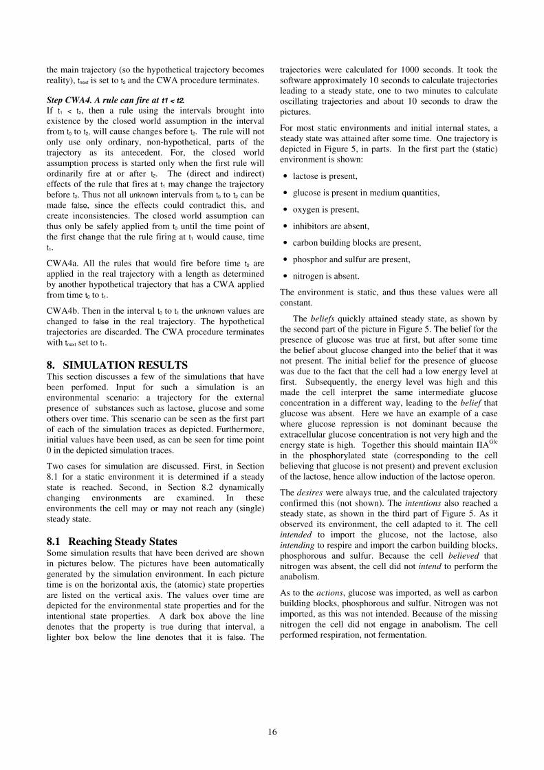
16

the main trajectory (so the hypothetical trajectory becomes reality), tnext is set to t2 and the CWA procedure terminates.

Step CWA4. A rule can fire at t1 < t2.

If t1 < t2, then a rule using the intervals brought into existence by the closed world assumption in the interval from t0 to t2, will cause changes before t2. The rule will not only use only ordinary, non-hypothetical, parts of the trajectory as its antecedent. For, the closed world assumption process is started only when the first rule will ordinarily fire at or after t2. The (direct and indirect) effects of the rule that fires at t1 may change the trajectory before t2. Thus not all unknown intervals from t0 to t2 can be made false, since the effects could contradict this, and create inconsistencies. The closed world assumption can thus only be safely applied from t0 until the time point of the first change that the rule firing at t1 would cause, time t1.

CWA4a. All the rules that would fire before time t2 are applied in the real trajectory with a length as determined by another hypothetical trajectory that has a CWA applied from time t0 to t1.

CWA4b. Then in the interval t0 to t1 the unknown values are changed to false in the real trajectory. The hypothetical trajectories are discarded. The CWA procedure terminates with tnext set to t1.

8. SIMULATION RESULTS This section discusses a few of the simulations that have been perfomed. Input for such a simulation is an environmental scenario: a trajectory for the external presence of substances such as lactose, glucose and some others over time. This scenario can be seen as the first part of each of the simulation traces as depicted. Furthermore, initial values have been used, as can be seen for time point 0 in the depicted simulation traces.

Two cases for simulation are discussed. First, in Section 8.1 for a static environment it is determined if a steady state is reached. Second, in Section 8.2 dynamically changing environments are examined. In these environments the cell may or may not reach any (single) steady state.

8.1 Reaching Steady States Some simulation results that have been derived are shown in pictures below. The pictures have been automatically generated by the simulation environment. In each picture time is on the horizontal axis, the (atomic) state properties are listed on the vertical axis. The values over time are depicted for the environmental state properties and for the intentional state properties. A dark box above the line denotes that the property is true during that interval, a lighter box below the line denotes that it is false. The

trajectories were calculated for 1000 seconds. It took the software approximately 10 seconds to calculate trajectories leading to a steady state, one to two minutes to calculate oscillating trajectories and about 10 seconds to draw the pictures.

For most static environments and initial internal states, a steady state was attained after some time. One trajectory is depicted in Figure 5, in parts. In the first part the (static) environment is shown:

• lactose is present,

• glucose is present in medium quantities,

• oxygen is present,

• inhibitors are absent,

• carbon building blocks are present,

• phosphor and sulfur are present,

• nitrogen is absent.

The environment is static, and thus these values were all constant.

The beliefs quickly attained steady state, as shown by the second part of the picture in Figure 5. The belief for the presence of glucose was true at first, but after some time the belief about glucose changed into the belief that it was not present. The initial belief for the presence of glucose was due to the fact that the cell had a low energy level at first. Subsequently, the energy level was high and this made the cell interpret the same intermediate glucose concentration in a different way, leading to the belief that glucose was absent. Here we have an example of a case where glucose repression is not dominant because the extracellular glucose concentration is not very high and the energy state is high. Together this should maintain IIAGlc in the phosphorylated state (corresponding to the cell believing that glucose is not present) and prevent exclusion of the lactose, hence allow induction of the lactose operon.

The desires were always true, and the calculated trajectory confirmed this (not shown). The intentions also reached a steady state, as shown in the third part of Figure 5. As it observed its environment, the cell adapted to it. The cell intended to import the glucose, not the lactose, also intending to respire and import the carbon building blocks, phosphorous and sulfur. Because the cell believed that nitrogen was absent, the cell did not intend to perform the anabolism.

As to the actions, glucose was imported, as well as carbon building blocks, phosphorous and sulfur. Nitrogen was not imported, as this was not intended. Because of the missing nitrogen the cell did not engage in anabolism. The cell performed respiration, not fermentation.

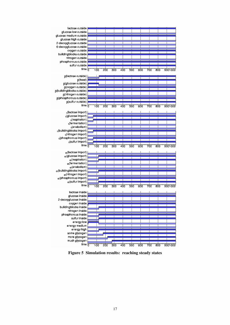
17

Figure 5 Simulation results: reaching steady states

18

The internal state of the cell was affected by the actions it took. At the very start the cell had a low energy status, but this soon changed to a high energy due to the import of nutrients and the absence of the (energy consuming) anabolism. Note that glucose inside was added for the first 300 seconds to provide initial energy for the cell to start. Nitrogen inside did not increase. Oxygen was present inside the cell by diffusing passively through the cell membrane.

It is shown in this trajectory that after about 300 seconds a state has been reached which remained unaltered till the end of times. A large variety of static environments have been tried in a similar manner. In most cases a steady state was reached. But in some cases the cell started to oscillate, this is shown in the next example simulation, which also deals with a fluctuating environment.

8.2 Non Steady-State Processes: Process

from one Steady State to Another One If the environment is not static, then the cell does not always relax to the neighborhood of a steady state. It may start to fluctuate between two steady states, or exhibit more complex behavior. To examine these possibilities some simulations have been performed.

First a simulation which is changing in a more quiet manner, where the cell shifts from one steady state to another is shown (Figure 6). In Section 8.3 a more complex trace is shown (Figure 7).

In this example, shown in Figure 6, there is lactose in the environment, no glucose and no inhibitors. Resources are abundant, oxygen, buildingblocks, phosphorous and sulfur. Nitrogen is lacking at the start, but is added at time 500. At time 1500 glucose is added, glucose is high outside. At time 3000 the inhibitor 6-deoxyglucose is added outside.

The beliefs represent the state outside the cell at first, lactose present, glucose absent, oxygen, buildingblocks, phosphorous and sulfur present, and nitrogen absent. The belief about a feast starts to hold, as the lack of glucose is compensated by high energy. As nitrogen is added, quickly the belief that nitrogen is present outside starts to hold. The belief about a feast stops holding after that. As the glucose is added outside, the belief in a feast starts holding again, as well as the belief that glucose is outside. The lactose can no longer be observed, the cell (falsely) believes that there is no lactose outside. After the inhibitor is added, after some small fluctuation the cell settles in a steady state where it can no longer observe the glucose due to the inhibitor. The cell believes that glucose is absent, there is no feast, and lactose is present outside. The desires all hold (not shown).

At first, the bacterium intends to grow on lactose. It intends to import lactose, and also glucose (constitutionally). As the bacterium believes there is

oxygen, it intends to respire and not ferment. The bacterium intends to import the buildingblocks, phosphorous and sulfur. The bacterium does not intend to import nitrogen, as it believes that nitrogen is absent outside. Since there is no nitrogen, the cell does not intend to perform the anabolism either. After the start, the cell no longer intends to import lactose, as it believes there is no famine. After nitrogen is added, the cell starts to intend to import the nitrogen, and also the cell intends to perform the anabolism. After that the cell intends to import lactose again, as the energy level has lowered, and there is no more belief about a feast. After the glucose is added outside, the cell no longer intends to import lactose. As the glucose uptake is inhibited at time 3000 the cell again intends to import lactose.

The actions are according to the intentions. At first the cell performs the import of lactose, respire, and the import of buildingblocks, phosphorous and sulfur. Slightly after that the cell performs the import of glucose as well, since it intends to. Some time after nitrogen is added to the environment, the cell performs the import of nitrogen and the anabolism. As the glucose is added at time 1500, the cell starts to perform glucose import as well, stopping the lactose import action some time later. When glucose uptake becomes inhibited, the cell switches back to taking up lactose, not glucose.

The internal state of the cell shows a start and the changes from a steady state to the next. At the start, glucose is inserted inside cell, and oxygen quickly appears. The energy is low, as no fermentation or respiration is done yet. After time 100, as the cell starts to perform actions, lactose becomes present inside, as well as the buildingblocks, phosphorous and sulfur. The energy switches to high, as the cell starts to respire. Some time after the nitrogen is added outside, nitrogen becomes present inside, and the energy level drops from high to medium as the anabolism is performed, lowering the energy level. After the glucose is added to the environment, the cell imports it almost immediately. The quick reaction is due to preparation by constitutionally expressing the glucose operon. As the glucose is suddenly inhibited at time 3000, the glycogen stores are used to restore energy as it suddenly drops to low. The cell then readjusts and lactose becomes present inside instead of glucose.

19

Figure 6 Simulation results: A process from one steady state to another steady state

20

8.3 Non Steady-State Processes: More

Complex Dynamics The more complex example trajectory (see Figure 7) presented is one where the environment had both a quickly changing glucose concentration, and a slowly changing oxygen concentration. Moreover, in this simulation, the environment contained no lactose, no inhibitors. N, P, S, and C building blocks were present. Oxygen was present at first and glucose oscillated between a medium and high concentration. Later, i.e., at time 500, the oxygen disappeared, and the glucose kept oscillating. At time 750 glucose was added.

In the simulation some state properties of the cell fluctuated when the oxygen was still present, notably the belief in the presence of glucose. When glucose was absent, the belief of lactose was present, and conversely. The belief in the presence of oxygen shifted from one steady state to another, as the oxygen was removed at time 500, and shifted back when oxygen was added again. The beliefs in building blocks, nitrogen, phosphorous and sulfur reached a stable steady state. The desires of the cell were all constant (not shown).

The simulated cell did not intend to import lactose. It intended to import glucose, building blocks, nitrogen, phosphorous and sulfur. The cell also intended to do the anabolism. At first, the cell intended to respire, and reached a corresponding steady state. After time 500, the cell took some time to adjust to intending to do the fermentation instead. A first, shorter steady state of about 30 seconds ensued where the cell intended to

perform both respiration and fermentation, even though there was no more oxygen. Maintaining the intention to

perform respiration should lead to a quicker performance of the respiration in case of returning oxygen in the environment, than if the respiration had to be prepared all over. The cell reached a new steady state at approximately 600 s, where it only intended the fermentation.

Slightly after time 500 s, the cell switched from respiration to fermentation. The respiration action did not cease since activated enzymes remained present for a long time, and meanwhile oxygen got added again, and the cell could quickly react, and immediately start using the returned oxygen. The fermentation took a short while to be prepared, and was then performed. The cell did not perform the import of lactose. It did perform the import of glucose, building blocks, nitrogen, phosphorous and sulfur. The cell performed the anabolism.

The internal state of the cell underwent some changes. There was no lactose. There were carbon building blocks, nitrogen, phosphorous and sulfur inside. There was no 2-deoxyglucose inside. The oxygen inside the cell quickly ran out as the oxygen in the environment was removed, and returned as oxygen was added to the environment of the cell. The energy level, low at the

very start, was medium while the respiration was taking place, dipped to low again as oxygen was removed but started to oscillate between low and medium as the cell tried to adapt to the anaerobic conditions. There was no high energy without oxygen as the fermentation had to be used (which is known to yield less ATP). Also, the glucose inside oscillated in phase with the energy. The oscillation repeated every 8 seconds. As oxygen was added to the cell the oscillation did not disappear – even though previously the cell had adapted to a short steady state with oxygen (before time 500). After time 750, high energy was used in the oscillation instead of medium energy:

Even though glucose fluctuated in the environment, the cell reached a steady state at first. Later it changed to adapt to external changes, but also began to oscillate internally as oxygen was removed. The oscillation stayed even when oxygen was added again.

In this example the cell managed to adapt itself to changes in the environment, and reached a steady state even when faced with sustained environmental fluctuations.

Other simulations have been performed (not shown), showing that the oscillation also occurs when glucose does not fluctuate in the environment. Additionally, the cell can switch from one steady state to the next, for example in a sulfur fluctuation every 500 seconds in the environment. The current example has been chosen, as it also shows the ability of the cell to keep a stable internal state in spite of external fluctuation.

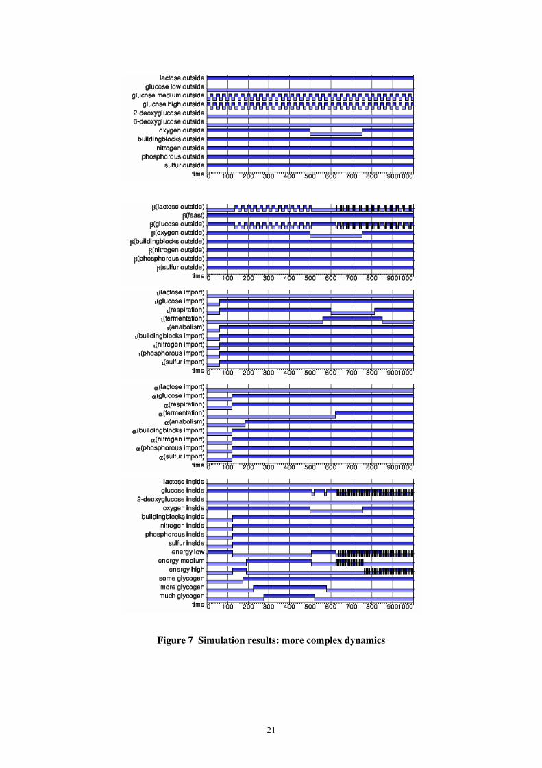
21

Figure 7 Simulation results: more complex dynamics

22

9 DISCUSSION Although in principle cellular processes can be described by hundreds to thousands of differential equations for the various chemical reactions, more abstract ways of describing the main paths of the processes, their regulation and their dynamics are desirable. Such abstractions can be developed in different manners. One manner, for example, is to use numerical models based on differential equations for ‘lumped’ sets of biochemical reactions. In this paper a different way to obtain a more abstract model was explored: a temporalised BDI-model, a model based on temporal relations between internal state properties such as beliefs, desires, and intentions.

The BDI-model is well-known in the literature on Artificial Intelligence and agent systems; cf. (Rao and Georgeff, 1991). The aim to explore in how far BDI-models can be exploited as a kind of template to model intracellular dynamics confronted us with the challenge of marrying a discrete, binary intentional decision process modelled within BDI-models to the continuous dynamics of (chemical) cellular processes in the real world. We consider as a main contribution of the paper that a bridge is provided between two areas in different disciplines in the scientific literature, namely cell modelling and BDI-modelling. Both areas are represented by large numbers of papers introducing specific research questions and techniques.

To allow transparent and executable specification of dynamical relations between intentional state properties, we needed a temporal version of the BDI-model, i.e., one in which temporal relationships can be defined between the different intentional state properties, and in relation to dynamic events in the external world. Based on the perspective put forward in (Finger and Gabbay, 1992), such an executable continuous time temporal modelling approach was introduced: the CTBDI-model, a continuous time extension of the BDI-model. In the processing of the CTBDI-model, a temporal simulation process replaces the inference process, which is usually applied to process the (non-temporalised) logic-based BDI-model.

In this paper the temporalised BDI-model has been followed as faithfully as possible, however this does not capture all intricacies. A simplification has been performed, by describing readiness as an active enzyme. In reality, transcription produces enzymes, possibly having some translational regulation. Then, these enzymes can be deactivated, in metabolic control. These two steps are taken as one in this paper, but for future research the extension of the model to more fully capture the cell regulation would be interesting.

Another simplification in this paper is the way in which reasons (to generate an intention for a given desire, or to generate an action initiation for a given intention) are treated. The reasons are a collection of suitable beliefs. In mammals, however, to make this work the reporter substances (the beliefs) have to bind to a repressor, which is perhaps not always present. This makes the regulation

more complex. This means that the computation of the combinations of beliefs takes time and perhaps additional resources too. The additional detail is useful and is a starting point for future research, in particular on how this process can be described by dynamics of intentional state properties.

This dynamic model combines discrete state properties (e.g., defined on the basis of threshold values) with a continuous time scale. Thus the approach bridges the gap between the continuous chemical and the discrete intentional perspective on cellular processes. This abstraction from the chemical details gives a good sight at the larger picture, but still shows the complex dynamics. The advantage being simplicity and proximity to intuition, there is of course a price: system properties are not described in terms of a continuous concentration scale; they are absent or present, with some gradation added if essential (e.g., the three possible states for the external glucose concentrations). This applies not only to steady state dynamics in relation to static environments, but also to more complex non-steady state dynamics in relation to dynamic environments.

The chemical details are not unimportant; they can merit a thorough investigation, and perhaps the method discussed in this paper can then aid by providing an overall perspective of the chemical details that are not under investigation. For this purpose a relationship between intentional state properties and chemical properties was defined. In this sense, nothing has really been lost. Whether cell biology lends itself to such a more discrete characterization, is still up in the air of the experimental laboratories.

A dynamic model of E. coli illustrated the applicability of this approach. The model enabled simulation of the cellular processes over time, without expensive integration of differential equations. A software environment has been created for specification and simulation, which also plots the simulation results. Validation of the model has taken place in two different manners. Firstly, by defining one to one correspondences between intentional state properties and chemical state properties, the dynamic relations between intentional states have been translated into dynamic relations between chemical states. These dynamic relations were in accordance with available knowledge about cell biochemistry. This validation procedure corresponds to the notion of (local) reduction in the Philosophy of Science; cf. (Nagel, 1961; Kim, 1996). The one-to-one correspondences between intentional and chemical state properties can be viewed as bridge principles. Validation as described then amounts to (locally) confirming Nagel’s conditions on reduction.

A second type of validation was performed by a number of simulation experiments. For static environments in most cases a steady state was reached, which is expected on the basis of knowledge on cell functioning. A large number of simulation experiments with dynamic environments have also been performed. Specifically, as

23

the model is not based on steady state assumptions, it allows for experiments with changing environments. The model showed robust performance in that after each environmental change it attempted to reach the appropriate new steady state. If the environmental changes were not too fast, such an intermediate steady state was reached. For environments that had fluctuations with high frequencies, in many cases the internal cell processes were able to become stable, due to internal effects that lasted longer than the periods without change in the outside world. All this observed behaviour seems highly plausible, in comparison to reports in the literature.

The value of work of this type lies in managing the complexity of living systems. For example, the internal processes within organisms often are so complex that explanations of their behavior in terms of a large variety of physical and chemical processes seemed inaccessible. This paper shows how, at least for moderately complex organisms, combined abstraction and intentionalisation of such continuous processes can be done in a justifiable manner. The resulting models show intentional dynamics realised in physical and chemical models of real world dynamics. Due to the high abstraction level of the models, simulation can be done within seconds, which highly encourages experimentation with the simulation program.2

As a basic vehicle underlying the BDI-models presented here, the causal temporal logical modelling approach based on the LEADSTO environment (Bosse et al., 2007) has been chosen. This choice is not defended to be the one and only choice possible. The paper demonstrates that this environment is a good possibility to build upon, but other possibilities, such as those based on kinetic logic (e.g., Thomas, 1973, 1979, 1990) may work as well. In fact any causal or temporal modelling approach in which timing and time delays can be expressed may do the job. The choice for LEADSTO among the different possibilities was based on secundary reasons only, such as: (1) among the authors there is much expertise on this language and the related tools, (2) a library of reusable models is set up for this language, given this, it is nice to include the model described here in this library as well, (3) models in the language LEADSTO can be smoothly related to models in the language TTL to allow logical verification, such as automatically checking properties of simulation traces; for more details on this, see: (Bosse, Jonker, Meij, Sharpanskykh, and Treur, 2006).

The main contribution of the paper is to show how on top of such a basic vehicle, the BDI-modelling approach can be worked out and used as a kind of template offered to the area of modelling intracellular dynamics, thus providing a bridge between two different scientific areas. This bridge may provide possibilities for researchers in both areas to introduce new research questions and new techniques, by going back and forth between the two areas.

2 For those who want to check the software, a request can be sent to the third author.

ACKNOWLEDGEMENTS The authors are grateful to the anonomous reviewers, whose comments have led to a more precise formulation of a number of the details, and of the motivation of the work.

REFERENCES Bakker, B.M., Michels, P.A.M., Opperdoes, F.R. and

Westerhoff, H.V. (1997) Glycolysis in bloodstream form Trypanosoma brucei can be understood in terms of the kinetics of the glycolytic enzymes. J. Biol. Chem. 272, 3207–3215.

Barringer, H., Fisher, M., Gabbay, D., Owens, R., and Reynolds, M. (1996). The Imperative Future: Principles of Executable Temporal Logic, Research Studies Press Ltd. and John Wiley & Sons.

Ben-Jacob, E., Cohen, I., Czirók, A., Vicsek, T., and Gutnick, D.L. (1997) Chemomodulation of Cellular Movement and Collective Formation of Vortices by Swarming Bacteria. In: Physica A, Vol. 238, pp. 181-197.

Bosse, T., Jonker, C.M., Meij, L. van der, and Treur, J., (2005). A Language and Environment for Analysis of Dynamics by SimulaTiOn. International Journal of Artificial Intelligence

Tools, vol. 16, 2007, pp. 435-464. Bosse, T., Jonker, C.M., Meij, L. van der, Sharpanskykh, A.,

and Treur, J., (2006). Specification and Verification of Dynamics in Cognitive Agent Models. In: Nishida, T., Klusch, M., Sycara, K., Yokoo, M., Liu, J., Wah, B., Cheung, W., and Cheung, Y.-M. (eds.), Proceedings of the Sixth

International Conference on Intelligent Agent Technology,

IAT'06. IEEE Computer Society Press, 2006, pp. 247-254. Bosse, T., Sharpanskykh, A., and Treur, J., (2007). Integrating

Agent Models and Dynamical Systems. In: Baldoni, M., Son, T.C., Riemsdijk, M.B. van, and Winikoff, M. (eds.), Proc. of

the 5th International Workshop on Declarative Agent

Languages and Technologies, DALT 2007, 2007, pp. 1-16. To be published by Springer Verlag. Abstract in Proc. of the

Sixth International Conference on Complex Systems, ICCS'06, 2006.

Bruckner, R. and Titgemeyer, F. (2002). Carbon catabolite repression in bacteria: choice of the carbon source and autoregulation limitation. FEMS Microbiol. Lett. 209:141-148.

Chaochen, Z., Hoare, C.A.R., and Ravn, A.P. (1991). A calculus of durations. In: Information Processing Letters, Vol. 40, pp. 269-276.

Clark, A. (1997). Being There: Putting Brain, Body and World

Together Again. MIT Press, 1997. Clark, A. (1999). Where brain, body, and world collide. Journal

of Cognitive Systems Research, 1, 1999, pp. 5-17. Dardenne, A., Lamsweerde, A. van, and Fickas, S. (1993). Goal-

directed Requirements Acquisition. Science in Computer

Programming, vol. 20, pp. 3-50. Darimont, R., and Lamsweerde, A. van (1996). Formal

Refinement Patterns for Goal-Driven Requirements Elaboration. Proceedings of the Fourth ACM Symposium on

the Foundation of Software Engineering (FSE4), pp. 179-190. Death, A., and Ferenci, T. (1994) Between Feast and Famine:

Endogenous Inducer Synthesis in the Adaptation of Escherichia coli to Growth with Limiting Carbohydrates. J Bacteriol 176:5101-5107

Dennett, D.C. (1987). The Intentional Stance. MIT Press. Cambridge Mass.

Dennett, D.C. (1991). Real Patterns. The Journal of Philosophy, vol. 88, 1991, pp. 27-51.

24

Dretske, F.I. (1988). Explaining Behaviour: Reasons in a World

of Causes. MIT Press, Cambridge, Massachusetts. Dubois, E., Du Bois, P., and Zeippen, J.M. (1995). A Formal

Requirements Engineering Method for Real-Time, Concurrent, and Distributed Systems. In: Proceedings of the

Real-Time Systems Conference, RTS’95. Elgot-Drapkin, J.J., and Perlis, D. (1990). Reasoning Situated in

Time I: Basic Concepts. In: Journal of Experimental and Theoretical Artificial Intelligence, Vol. 2, pp. 75-98.

Finger, M., and Gabbay, D. (1992). Adding a temporal dimension to a logic system, Journal of Logic, Language and

Information, vol. 1, pp. 203-233. Fisher, M., (1994). A survey of Concurrent METATEM — the

language and its applications. In: D.M. Gabbay, H.J. Ohlbach (eds.), Temporal Logic — Proceedings of the First

International Conference, Lecture Notes in AI, vol. 827, pp. 480–505.

Fisher, M., (2005). Temporal Development Methods for Agent-Based Systems, Journal of Autonomous Agents and Multi-

Agent Systems, vol. 10, 2005, pp. 41-66. Galton, A. (2003). Temporal Logic. Stanford Encyclopedia of

Philosophy, URL: http://plato.stanford.edu/entries/logic-temporal/#2.

Galton, A. (2006). Operators vs Arguments: The Ins and Outs of Reification. Synthese, vol. 150, 2006, pp. 415-441.

Gear, C.W., (1971). Numerical Initial Value Problems in Ordinary Differential Equations. Englewood Cliffs, NJ: Prentice-Hall.

Flikweert, M.T., Van Dijken, J.P., and Pronk, J.T. (1997). Metabolic responses of pyruvate-decarboxylase-negative Saccharomyces cerevisiae to glucose excess. In: Applied and

environmental Microbiology, Vol. 63, pp. 3399-3404. Geert, P. van (1991). A dynamic systems model of cognitive and

language growth. Psychological Review, vol. 98, pp. 3-56. Geert, P. van (1995). Growth Dynamics in Development. In:

(Port and van Gelder, 1995), pp. 101-120. Heinrich, R. and Schuster, S. (1996) The Regulation of Cellular

Systems, Chapman & Hall, New York, USA. Hutchison, C.A., Peterson, S.N., Gill, S.R., Cline, R.T., White,

O., Fraser, C.M., Smith, H.O., and Venter, J.C. (1999). Global transposon mutagenesis and a minimal Mycoplasma genome. Science, 1999 Dec 10; 286(5447): 2165-9.

Hynne F, Dano S, Sorensen PG., (2001). Full-scale model of

glycolysis in Saccharomyces cerevisiae. Biophys. Chem.,

volume 94, issue 1-2, pp. 121-63. Jonker, C.M., Snoep, J.L. Treur, J., Westerhoff, H.V,. and

Wijngaards, W.C.A. (2002). Putting Intentions into Cell Biochemistry: An Artificial Intelligence Perspective. Journal

of Theoretical Biology, vol. 214, pp. 105-134. Jonker, C.M., Treur, J., and Wijngaards, W.C.A., A Temporal

Modelling Environment for Internally Grounded Beliefs, Desires and Intentions. Cognitive Systems Research Journal, vol. 4(3), 2003, pp. 191-210.

Kahn, D., and Westerhoff, H.V. (1991). Control theory of regulatory cascades. J. Theor Biol. 1991 Nov 21; 153(2): 255-85.

Kelso, J.A.S. (1995). Dynamic Patterns: the Self-Organisation

of Brain and Behaviour. MIT Press, Cambridge, Mass. Kholodenko, B.N, Demin, O.V., Moehren, G., and Hoek, J.B.

(1999). Quantification of short term signaling by the epidermal growth factor receptor. J Biol Chem. 1999 Oct 15; 274(42): 30169-81.

Kim, J. (1996). Philosophy of Mind, Westview Press, 1996. Mendes, P. (1997), Biochemistry by numbers: simulation of

biochemical pathways with Gepasi 3. In: Trends Biochem.

Sci. Vol. 22, pp. 361-363. URL: http://www.gepasi.org/.

Moller K, Christensen B, Forster J, Piskur J, Nielsen J, and Olsson L. (2002). Aerobic glucose metabolism of Saccharomyces kluyveri: Growth, metabolite production, and quantification of metabolic fluxes. Biotechnol Bioeng. 2002 Jan 20;77(2):186-93.

Morin P.J, 1999. Community Ecology. Blackwell Publishing,

USA. Mulquiney, P.J., and Kuchel, P.W. (1999). Model of 2,3-

bisphosphoglycerate metabolism in the human erythrocyte based on detailed enzyme kinetic equations: computer simulation and metabolic control analysis. Biochem J. 1999 Sep 15; 342 Pt 3: 597-604.

Nagel, E. (1961). The Structure of Science. Harcourt, Brace & World, New York.

Neidhardt, F.C., Curtiss III, R., Ingraham, J.L., Lin, E.C.C., Brooks Low, K., Magasanik, B., Reznikoff, W.S., Riley, M., Schaechter, M., and Umbarger, H.E., eds. (1996). Escherichia

coli and Salmonella typhimurium. ASM Press, Washington, D.C.

Port, R.F., and Gelder, T. van (eds.) (1995). Mind as Motion:

Explorations in the Dynamics of Cognition. MIT Press, Cambridge, Mass.

Press, W. H., Teukolsky, S. A., Vetterling,W. T., and Flannery,

B. P., 1992. Numerical recipes in C: the art of scientific

computing. Cambridge university press, second edition. Rao, A.S., and Georgeff, M.P. (1991). Modelling Rational

Agents within a BDI-Architecture. In: J. Allen, R. Fikes and E. Sandewall, eds., Proceedings of the Second International

Conference on Principles of Knowledge Representation and

Reasoning, (KR’91), Morgan Kaufmann, 1991, pp. 473-484. Rizzi, M., Baltes, M., Theobald, U., and Reuss, M. (1997) In

vivo analysis of metabolic dynamics in Saccharomyces

cerevisiae: II. Mathematical model. Biotechnol. Bioeng. 55, 592–608.

Rohwer, J.M., Jensen, P.R., Shinohara, Y., Postma, P.W., and Westerhoff, H.V. (1996a). Changes in the cellular energy state affect the activity of the bacterial phosphotransferase system. Eur J Biochem. 1996a Jan 15;235(1-2):225-30.

Rohwer, J.M., Schuster, S., and Westerhoff, H.V. (1996b). How to recognize monofunctional units in a metabolic system. J

Theor Biol. 1996b Apr 7;179(3):213-28. Rohwer, J.M., Postma, P.W., Kholodenko, B.N., and

Westerhoff, H.V. (1998). Implications of macromolecular crowding for signal transduction and metabolite channeling. Proc Natl Acad Sci USA. 1998 Sep 1; 95(18): 10547-52.

Rohwer, J.M., Meadow, N.D., Roseman, S., Westerhoff, H.V., and Postma, P.W. (2000). Understanding glucose transport by the bacterial phosphoenolpyruvate: glycose phosphotransfer-ase system on the basis of kinetic measurements in vitro. J

Biol Chem. 2000 Nov 10; 275(45): 34909-21. Sandewall, E. (1997). Logic-Based Modelling of Goal-Directed

Behavior. In: Linköping Electronic Articles in Computer and

Information Science. Vol. 2, number 19. Schilling, C.H., Letscher, D., and Palsson, B. Ø. (2000). Theory

for the Systemic definition of Metabolic Pathways and their use in Interpreting Metabolic Function from a Pathway-Oriented Perspective. In: Journal of Theoretical Biology, Vol. 203, pp. 229-248.

Sloman, A., and Poli, R. (1995), SIM_AGENT: A toolkit for exploring agent designs, In: Wooldridge, W., Mueller, J., and Tambe, M. (eds.) Intelligent Agents Volume II (ATAL-95), Springer-Verlag, pp. 392-407.

Stock, J. B., Waygood, E. B., Meadow, N. D., Postma, P. W., and Roseman, S. (1982) Sugar Transport by the Bacterial Phosphotransferase System. J. Biol. Chem. 257, 14543–14552

25

Sun, R. (2000). Symbol grounding: a new look at an old idea. Philosophical Psychology, 13, 2000, pp. 149-172.

Teusink, B., Passarge, J., Reijenga, C.A., Esgalhado, E., van der Weijden, C.C., Schepper, M., Walsh, M.C., Bakker, B.M., van Dam, K., Westerhoff, H.V., and Snoep, J.L. (2000). Can yeast glycolysis be understood in terms of in vitro kinetics of the constituent enzymes? Testing biochemistry. Eur J

Biochem. 2000 Sep; 267(17):5313-29. Thomas, R. (ed.) (1979). Kinetic logic: a Boolean approach to

the analysis of complex regulatory systems, Lecture notes in Biomathematics. Springer-Verlag.

Thomas, R. (1973). Boolean formulization of genetic control circuits. Journal of Theoretical Biology 42: 565–583.

Thomas, R. (1991). Regulatory networks seen as asynchronous automata: A logical description. Journal of Theoretical

Biology, 1991, 153, 1-23.

Townsend, J.T., and Busemeyer, J. (1995). Dynamic

Representation in Decision Making. In: (Port and van Gelder, 1995), pp. 101-120.

Wang, J., Gilles, E.D., Lengeler, J.W., and Jahreis, K. (2001). Modeling of inducer exclusion and catabolite repression based on a PTS-dependent sucrose and non-PTS-dependent glycerol transport systems in Escherichia coli K-12 and its experimental verification. J Biotechnol. 2001 Dec 28;92(2):133-58.

Rotterdam, B.J. van, Crielaard, W., Stokkum, I.H. van, Hellingwerf, K.J., and Westerhoff, H.V. (2002). Simplicity in complexity: the photosynthetic reaction center performs as a simple 0.2 V battery. FEBS Lett. 2002 Jan 2;510(1-2):105-7.

Van Workum, M and Van Dooren, SJM and Oldenburg, N and Molenaar, D and Jensen, PR and Snoep, JL and Westerhoff, HV (1996) Mol Microbiol, 20:351-360

Visser, D., Heijden, R. van der, Mauch, K., Reuss, M., and Heijnen, S. (2002). Tendency modeling: a new approach to obtain simplified kinetic models of metabolism applied to Saccharomyces cerevisiae. Metab Eng. 2000 Jul; 2(3): 252-75.

Warner, J.B., and Lolkema, J.S. (2003). CcpA-Dependent carbon catabolite repression in bacteria. Microbiol. Mol. Biol. Rev. 67: 475-490.

West, A.H. and Stock, A.M. (2001). Histidine kinase and response regulation proteins in two-component signalling systems. Trends Biochem. Sci. 26: 369-376.

Westerhoff, H.V. (2001). The silicon cell, not dead but live! Metab Eng., Jul; 3(3):207-10.

Westerhoff, H.V. and Dam, K. van (1987). Thermodynamics and Control of Biological Free-Energy Transduction, Elsevier, Amsterdam.

Wright, B.E. and Albe, K.R. (1994). Carbohydrate metabolism in Dictyostelium discoideum: I. Model construction. J. Theor.

Biol. 169, 231–241.