VENKATESHWARA OPEN UNIVERSITY www.vou.ac.in MATHEMATICS-I BCA [BCA-102]

Welcome message from author
This document is posted to help you gain knowledge. Please leave a comment to let me know what you think about it! Share it to your friends and learn new things together.
Transcript
MATHEMATICS-I
VENKATESHWARAOPEN UNIVERSITY
www.vou.ac.in
VENKATESHWARAOPEN UNIVERSITY
www.vou.ac.in
MATHEMATICS-I
BCA[BCA-102]
MATHEM
ATICS -I
12 MM
MATHEMATICS-I
BCA
[BCA-102]
Authors:
V.K. Khanna & S.K. Bhambri: Units (1.0-1.2.3, 1.4-1.5.2, 1.8-1.13, unit-2 & 4)
Copyright © V.K. Khana & S.K. Bhambri, 2010
G.S. Monga: Units (1.3-1.3.5, 1.6-1.7, unit -3) Copyright © G.S. Monga, 2010
Vikas Publishing: Units (5) Copyright © Reserved, 2010
Reprint 2010
BOARD OF STUDIES
Prof Lalit Kumar SagarVice Chancellor
Dr. S. Raman IyerDirectorDirectorate of Distance Education
SUBJECT EXPERT
Prof. Saurabh Upadhya Dr. Kamal UpretiMr. Animesh Srivastav Hitendranath Bhattacharya
ProfessorAssociate ProfessorAssociate ProfessorAssistant Professor
CO-ORDINATOR
Mr. Tauha KhanRegistrar
All rights reserved. No part of this publication which is material protected by this copyright noticemay be reproduced or transmitted or utilized or stored in any form or by any means now known orhereinafter invented, electronic, digital or mechanical, including photocopying, scanning, recordingor by any information storage or retrieval system, without prior written permission from the Publisher.
Information contained in this book has been published by VIKAS® Publishing House Pvt. Ltd. and hasbeen obtained by its Authors from sources believed to be reliable and are correct to the best of theirknowledge. However, the Publisher and its Authors shall in no event be liable for any errors, omissionsor damages arising out of use of this information and specifically disclaim any implied warranties ormerchantability or fitness for any particular use.
Vikas® is the registered trademark of Vikas® Publishing House Pvt. Ltd.
VIKAS® PUBLISHING HOUSE PVT LTDE-28, Sector-8, Noida - 201301 (UP)Phone: 0120-4078900 Fax: 0120-4078999Regd. Office: A-27, 2nd Floor, Mohan Co-operative Industrial Estate, New Delhi 1100 44Website: www.vikaspublishing.com Email: [email protected]
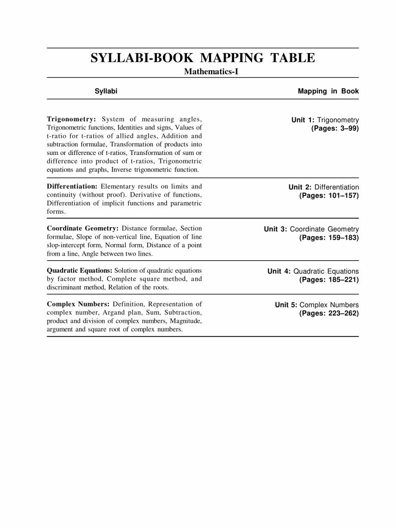
Trigonometry: System of measuring angles,
Trigonometric functions, Identities and signs, Values of
t-ratio for t-ratios of allied angles, Addition and
subtraction formulae, Transformation of products into
sum or difference of t-ratios, Transformation of sum or
difference into product of t-ratios, Trigonometric
equations and graphs, Inverse trigonometric function.
Differentiation: Elementary results on limits and
continuity (without proof). Derivative of functions,
Differentiation of implicit functions and parametric
forms.
Coordinate Geometry: Distance formulae, Section
formulae, Slope of non-vertical line, Equation of line
slop-intercept form, Normal form, Distance of a point
from a line, Angle between two lines.
Quadratic Equations: Solution of quadratic equations
by factor method, Complete square method, and
discriminant method, Relation of the roots.
Complex Numbers: Definition, Representation of
complex number, Argand plan, Sum, Subtraction,
product and division of complex numbers, Magnitude,
argument and square root of complex numbers.
Unit 1: Trigonometry(Pages: 3–99)
Unit 2: Differentiation(Pages: 101–157)
Unit 3: Coordinate Geometry
(Pages: 159–183)
Unit 4: Quadratic Equations(Pages: 185–221)
Unit 5: Complex Numbers(Pages: 223–262)
SYLLABI-BOOK MAPPING TABLEMathematics-I
Syllabi Mapping in Book

CONTENTS
INRODUCTION 1
UNIT 1 TRIGONOMETRY 3–99
1.0 Introduction
1.1 Unit Objectives1.2 System of Measuring Angles
1.2.1 Angles1.2.2 Measurement of Angles
1.2.3 Relations between the Three Systems of Measurements
1.3 Trigonometric Functions1.3.1 Periodic Functions
1.3.2 Trigonometric Ratios1.3.3 Values of Trigonometric Functions of Standard Angles
1.3.4 Signs of Trigonometric Ratios1.3.5 Fundamental Period and Phase
1.4 Identities and Signs1.4.1 Signs of Trigonometric Ratios
1.5 Trigonometric Ratios of Angles1.5.1 Standard Angles
1.5.2 Trigonometric Ratios of Allied Angles
1.6 Inverse Trigonometric Functions1.6.1 Range of Trigonometric Functions1.6.2 Properties of Inverse Trigonometric Functions
1.7 Trigonometric Equations1.8 Transformation of Trigonometric Ratios of Sums, Differences and Products1.9 Summary
1.10 Key Terms1.11 Answers to ‘Check Your Progress’1.12 Questions and Exercises1.13 Further Reading
UNIT 2 DIFFERENTIATION 101–157
2.0 Introduction2.1 Unit Objectives2.2 Limits and Continuity (Without Proof)
2.2.1 Functions and their Limits2.2.2 h-Method for Determining Limits
2.2.3 Expansion Method for Evaluating Limits2.2.4 Continuous Functions
2.3 Differentiation and Differential Coefficient2.4 Derivatives of Functions
2.4.1 Algebra of differentiable Functions
2.4.2 Differential Coefficients of Standard Functions2.4.3 Chain Rule of Differentiation
2.5 Derivatives: Tangent and Normal2.6 Differentiation of Implicit Functions and Parametric Forms
2.6.1 Parametric Differentiation
2.6.2 Logarithmic Differentiation
2.6.3 Successive Differentiation
2.7 Partial Differentiation2.8 Maxima and Minima of Functions2.9 Summary
2.10 Key Terms2.11 Answers to ‘Check Your Progress’2.12 Questions and Exercises2.13 Further Reading
UNIT 3 COORDINATE GEOMETRY 159–183
3.0 Introduction3.1 Unit Objectives3.2 Coordinate Geometry: An Introduction
3.2.1 The Distance Formula3.2.2 Midpoint of a Line Segment
3.3 Section Formula: Division of Lines3.3.1 Internal Division3.3.2 External Division
3.4 Equation of a Line in Slope-Intercept Form3.4.1 Variations of Slope-Intercept Form
3.5 Equation of a Line in Normal Form3.5.1 Angle between Two Lines3.5.2 Families of Parallel Lines
3.6 Distance of a Point From a Line3.6.1 Area of a Triangle
3.7 Summary3.8 Key Terms3.9 Answers to ‘Check Your Progress’
3.10 Questions and Exercises3.11 Further Reading
UNIT 4 QUADRATIC EQUATIONS 185–221
4.0 Introduction
4.1 Unit Objectives
4.2 Quadratric Equation: Basics4.2.1 Method of Solving Pure Quadratic Equations
4.3 Solving Quadratic Equations4.3.1 Method of Factorization
4.3.2 Method of Perfect Square
4.4 Discriminant Method and Nature of Roots
4.5 Relation of the Roots4.5.1 Symmetric Expression of Roots of a Quadratic Equation
4.5.2 Simultaneous Equations in Two Unknowns
4.5.3 Simultaneous Equations in Three or More than Three Unknowns
4.6 Summary
4.7 Key Terms
4.8 Answers to ‘Check Your Progress’
4.9 Questions and Exercises
4.10 Further Reading
UNIT 5 COMPLEX NUMBERS 223–262
5.0 Introduction
5.1 Unit Objectives
5.2 Imaginary Numbers
5.2.1 Definition of Complex Number
5.3 Complex Numbers: Basic Characteristics
5.3.1 Geometric Representation of Complex Numbers
5.3.2 Complex Arithmetic
5.3.3 Operations on Complex Numbers
5.3.4 Graphical Representation
5.3.5 Quadratic Functions and their Graphs
5.3.6 Polynomial Functions and their Graphs
5.3.7 Division of Univariate Polynomials
5.3.8 Zeros of Polynomial Functions
5.3.9 Rational Functions and their Graphs
5.3.10 Polynomial and Rational Inequalities
5.4 Uses of Complex Numbers
5.4.1 History of Complex Numbers
5.4.2 Geometrical Representation of Conjugates
5.4.3 Geometric Interpretation of Addition and Multiplication Operations
5.4.4 Matrix Representation of Complex Numbers
5.5 Properties of Complex Numbers
5.5.1 Applications of Complex Numbers
5.5.2 Signal Analysis
5.6 Summary
5.7 Key Terms
5.8 Answers to ‘Check Your Progress’
5.9 Questions and Exercises
5.10 Further Reading

Introduction
NOTES
Self-Instructional Material 1
INTRODUCTION
Mathematics is taught as a core subject in almost all undergraduate courses in
applied sciences, especially management and computer science. It is now generally
accepted that a study of any course is incomplete without the knowledge of
mathematics. Due to unfounded fear of the so called ‘difficult’ mathematics, students
tend to shy away from the subject and often, it becomes difficult to persuade them
to take special courses in mathematics. However, the fact is that learning to use
mathematical techniques does not require elaborate mathematical preparation and
the student need not be dismayed by some mathematical manipulations. One learns
through practice. Mathematics is best learnt through systematic learning. The learner
is bound to find it rewarding and exciting, while following the logical arguments
and steps involved.
Mathematics-I is a suitable textbook for the students of BCA. Topics,
such as trigonometry, differentiation, coordinate geometry, quadratic equations
and complex numbers, have been covered in detail in this book.
This book gives a simple and clear presentation of mathematics which will
be useful to beginners. There is a fairly self-contained development of the topics
and the student will find here a starting point which will help gain self-confidence
and familiarity with the subject. While the knowledge of elementary mathematics
is assumed, an attempt has been made to explain simple terms also. The student
will attain proficiency in mathematics, while he proceeds further with different
aspects of his studies.
The book follows the self-instructional mode wherein each unit begins with
an Introduction to the topic. The Unit Objectives are then outlined before going on
to the presentation of the detailed content in a simple and structured format. Check
Your Progress questions are provided at regular intervals to test the student’s
understanding of the topics. A Summary, a list of Key Terms and a set of Questions
and Exercises are provided at the end of each unit for recapitulation.

Trigonometry
NOTES
Self-Instructional Material 3
UNIT 1 TRIGONOMETRY
Structure
1.0 Introduction1.1 Unit Objectives1.2 System of Measuring Angles
1.2.1 Angles
1.2.2 Measurement of Angles1.2.3 Relations between the Three Systems of Measurements
1.3 Trigonometric Functions1.3.1 Periodic Functions1.3.2 Trigonometric Ratios
1.3.3 Values of Trigonometric Functions of Standard Angles1.3.4 Signs of Trigonometric Ratios
1.3.5 Fundamental Period and Phase
1.4 Identities and Signs1.4.1 Signs of Trigonometric Ratios
1.5 Trigonometric Ratios of Angles1.5.1 Standard Angles1.5.2 Trigonometric Ratios of Allied Angles
1.6 Inverse Trigonometric Functions1.6.1 Range of Trigonometric Functions1.6.2 Properties of Inverse Trigonometric Functions
1.7 Trigonometric Equations1.8 Transformation of Trigonometric Ratios of Sums, Differences and Products1.9 Summary
1.10 Key Terms1.11 Answers to ‘Check Your Progress’1.12 Questions and Exercises1.13 Further Reading
1.0 INTRODUCTION
Trigonometry is that branch of Mathematics which deals with the measurement of
angles. It is derived from two Greek words ‘trigonon’ (a triangle) and ‘metron’
(a measure), thereby meaning measurement of triangles. However, now this
definition has been modified to include measurement of angles in general, whetherthe angles are of a triangle or not. In this unit, you will learn about plane trigonometry
which is restricted to the measurement of angles in a plane.
Trigonometry is related to the calculation of sides and angles of triangleswith the help of trigonometric functions. The most familiar trigonometric functions
are the sine, cosine and tangent. Trigonometric functions were primarily employed
in mathematical tables.
In this unit, you will learn to measure angles and use trigonometric functions.
In addition, you will be introduced to signs and identities along with the standard
ratios of commonly used angles. Finally, this unit will deal with the complex
trigonometric calculations and computing.
4 Self-Instructional Material
Trigonometry
NOTES
1.1 UNIT OBJECTIVES
After going through this unit, you will be able to:
• Understand the various ways of measuring angles in a plane
• Explain the various trigonometric functions and use these applications to
solve problems related to angles
• Understand the concepts of identities and signs
• Discover and prove the trigonometric ratios of the standard as well as allied
angles
• Understand the various features of inverse trigonometric functions
• Comprehend and resolve trigonometric equations
• Modify trigonometric ratios of basic computing
1.2 SYSTEM OF MEASURING ANGLES
1.2.1 Angles
An angle is defined as the rotation of a line on one of its extremities in a plane from
one position to another. Two lines are said to be at right angles, if a revolving linestarting from one position to another describes a quarter of a circle. In case therevolving line moves in anticlockwise direction, then the angle described by it is
positive, else, it is negative. There is no limitation to the size of angles in trigonometry.
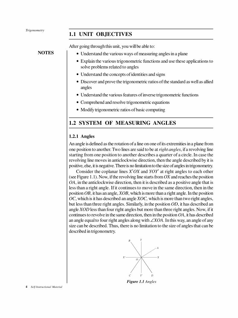
Consider the coplanar lines X′OX and YOY′ at right angles to each other(see Figure 1.1). Now, if the revolving line starts from OX and reaches the position
OA, in the anticlockwise direction, then it is described as a positive angle that isless than a right angle. If it continues to move in the same direction, then in theposition OB, it has an angle, XOB, which is more than a right angle. In the positionOC, which is it has described an angle XOC, which is more than two right angles,
but less than three right angles. Similarly, in the position OD, it has described anangle XOD less than four right angles but more than three right angles. Now, if itcontinues to revolve in the same direction, then in the position OA, it has describedan angle equal to four right angles along with ∠XOA. In this way, an angle of any
size can be described. Thus, there is no limitation to the size of angles that can be
described in trigonometry.
XX'O
Y'C D
YB
A
Figure 1.1 Angles
Trigonometry
NOTES
Self-Instructional Material 5
Quadrants
The four portions XOY, X′OY, X′OY′ and XOY′ into which a plane is divided are
called first, second, third and fourth quadrants respectively.
1.2.2 Measurement of Angles
To measure angles, a particular angle is fixed and is taken as a unit of measurement,
so that any other angle is measured by the number of times it contains the unit. For
example, if ∠XOY is a right angle, and it is taken as a unit of measurement, then
∠XOX′ is equal to two right angles, as it contains two units.
You will study the following three systems of measurement:
1. Sexagesimal System (English System)
2. Centesimal System (French System)
3. Circular System
1. Sexagesimal System: In this system, a right angle is divided into 90 equal
parts called degrees. Each degree is divided into 60 equal parts called minutes
and each minute is further, subdivided into 60 equal parts called seconds.
Thus, 1 right angle = 90 degrees
1 degree = 60 minutes
1 minute = 60 seconds.
In symbols, a degree, a minute and a second are respectively written as 1º; 1′,
1′′. Thus, 40º 15′ 20′′ denotes the angle which contains 40 degrees 15 minutes
and 20 seconds. The unit of measurement in this system is degree. This system is
called sexagesimal because each unit is divided into 60 parts (sexagesimus means
sixtieth) so that number 60 comes which marking the divisions.
2. Centesimal System: In this system, a right angle is divided into 100 equal
parts called grades. Each grade is divided into 100 equal parts called minutes
and each minute is divided into 100 equal parts called seconds.
Thus, 1 right angle = 100 grades
1 grade = 100 minutes
1 minute = 100 seconds
In this system the symbols 1g, 1̀, 1̀` stand for a grade, a minute and a
second respectively. Thus, 20g 12̀ 85̀ ` denotes the angle which contains 20 grades
12 minutes and 85 seconds. The unit of measurement here is grade. This system is
called centesimal system because the number 100 comes in marking the divisions
(centesimus means hundredth).
Note. The reader should observe the difference in notations of minutes
and seconds in the Sexagesimal and Centesimal systems.
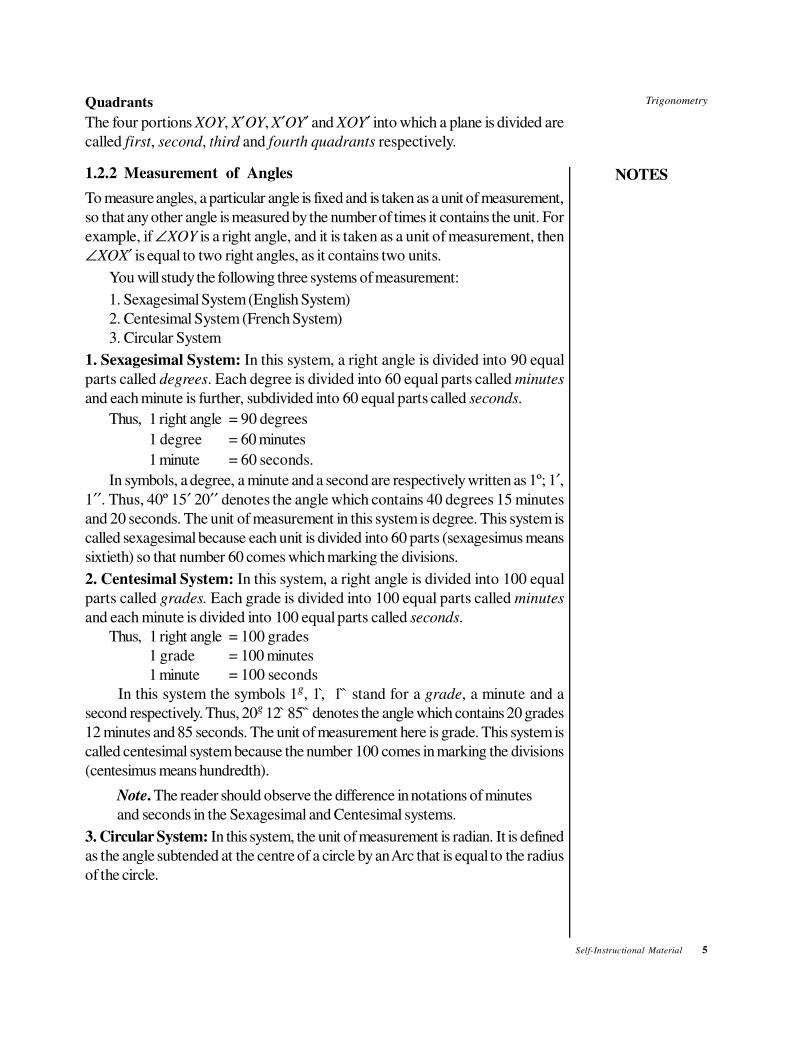
3. Circular System: In this system, the unit of measurement is radian. It is defined
as the angle subtended at the centre of a circle by an Arc that is equal to the radius
of the circle.
6 Self-Instructional Material
Trigonometry
NOTES
Consider a circle with centre O. Take any point A on it and cut off an Arc AB
that has a length, equal to the radius of the circle. Then, ∠AOB is called a radian
(see Figure 1.2).
The symbol 1c denotes a radian.
OA
B
Figure 1.2 Radian Angle
It is well known that ‘The circumference of a circle bears a constant
ratio to its diameter.’
This constant ratio is denoted by the Greek letter π (pronounced as ‘pie’).
The value of π correct upto two places of decimal is 3.14 equivalent to 22
7
and upto six places of decimal is 3.141593, equivalent to 355
113.
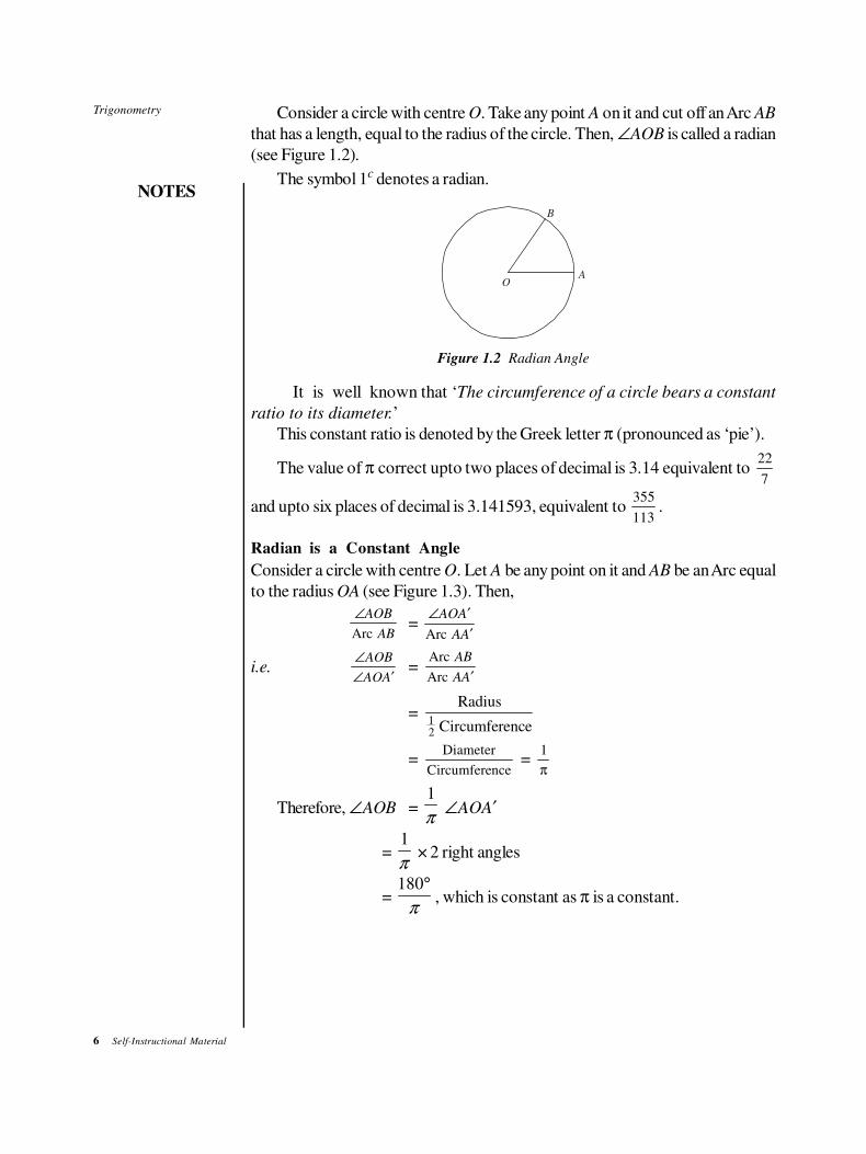
Radian is a Constant Angle
Consider a circle with centre O. Let A be any point on it and AB be an Arc equal
to the radius OA (see Figure 1.3). Then,
∠AOB
ABArc=
∠ ′
′
AOA
AAArc
i.e.∠
∠ ′
AOB
AOA=
Arc
Arc
AB
AA′
= 12
Radius
Circumference
= Diameter
Circumference =
1
π
Therefore, ∠AOB = 1
π ∠AOA′
= 1
π × 2 right angles
= 180
π
°, which is constant as π is a constant.
Trigonometry
NOTES
Self-Instructional Material 7
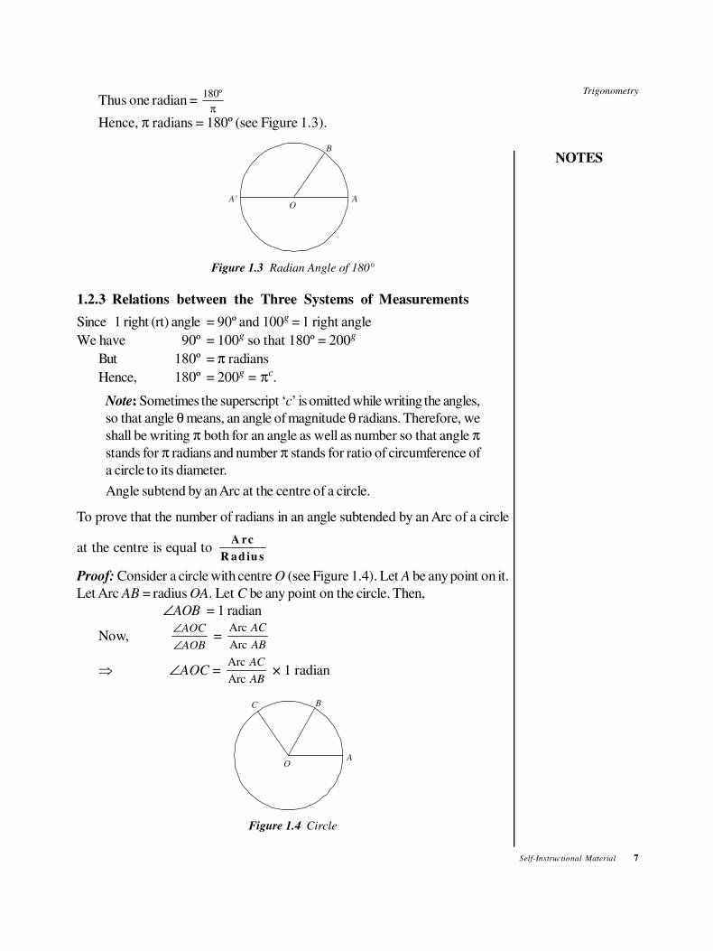
Thus one radian = 180º
π
Hence, π radians = 180º (see Figure 1.3).
OAA'
B
Figure 1.3 Radian Angle of 180°
1.2.3 Relations between the Three Systems of Measurements
Since 1 right (rt) angle = 90º and 100g = 1 right angle
We have 90º = 100g so that 180º = 200g
But 180º = π radians
Hence, 180º = 200g = πc.
Note: Sometimes the superscript ‘c’ is omitted while writing the angles,
so that angle θ means, an angle of magnitude θ radians. Therefore, we
shall be writing π both for an angle as well as number so that angle π
stands for π radians and number π stands for ratio of circumference of
a circle to its diameter.
Angle subtend by an Arc at the centre of a circle.
To prove that the number of radians in an angle subtended by an Arc of a circle
at the centre is equal to A rc
R ad iu s
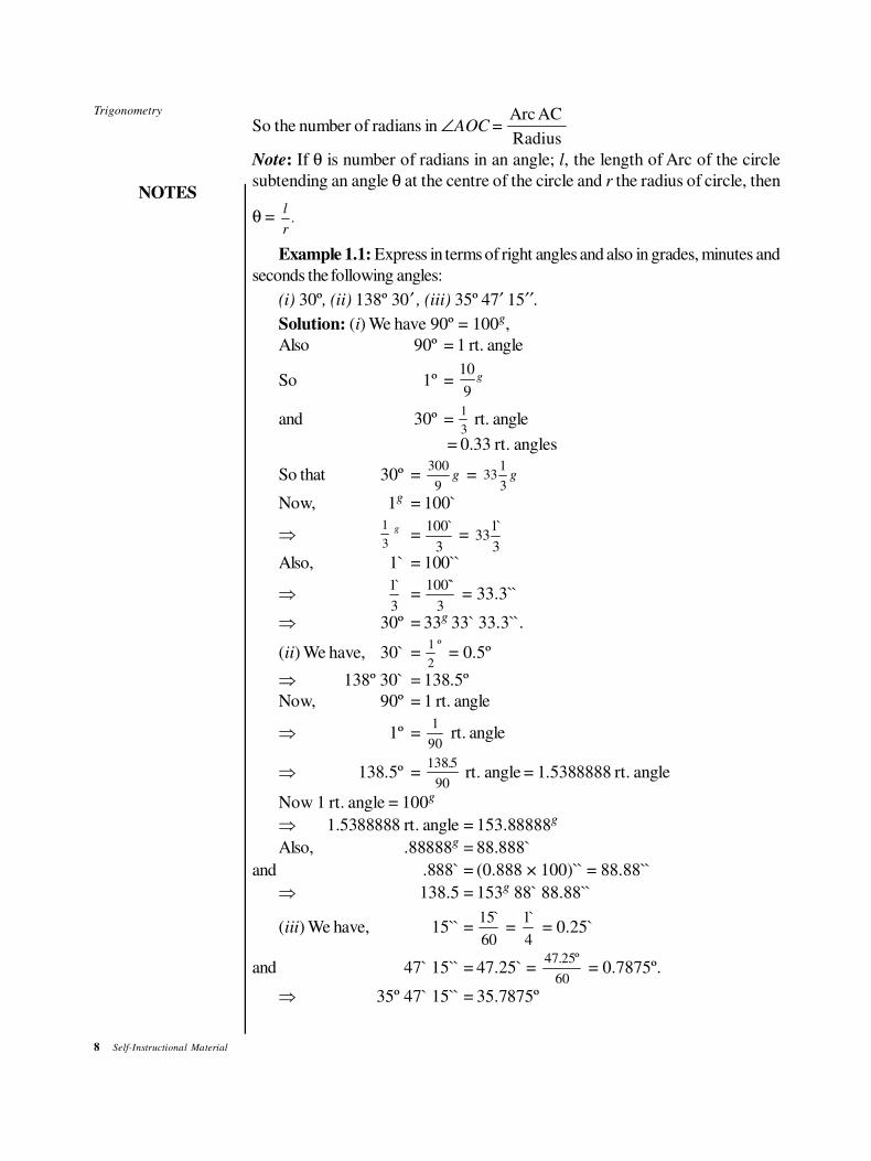
Proof: Consider a circle with centre O (see Figure 1.4). Let A be any point on it.
Let Arc AB = radius OA. Let C be any point on the circle. Then,
∠AOB = 1 radian
Now, ∠
∠
AOC
AOB =
Arc
Arc
AC
AB
⇒ ∠AOC = Arc
Arc
AC
AB × 1 radian
OA
BC
Figure 1.4 Circle
8 Self-Instructional Material
Trigonometry
NOTES
So the number of radians in ∠AOC = Arc AC
Radius
Note: If θ is number of radians in an angle; l, the length of Arc of the circle
subtending an angle θ at the centre of the circle and r the radius of circle, then
θ = .l
r
Example 1.1: Express in terms of right angles and also in grades, minutes and
seconds the following angles:
(i) 30º, (ii) 138º 30 ′ , (iii) 35º 47′ 15′′.
Solution: (i) We have 90º = 100g,
Also 90º = 1 rt. angle
So 1º =10
9g
and 30º =1
3 rt. angle
= 0.33 rt. angles
So that 30º =300
9g = 33
1
3g
Now, 1g = 100`
⇒1
3
g=
100`
3 =
1̀33
3Also, 1` = 100`̀
⇒1̀
3=
100`̀
3 = 33.3`̀
⇒ 30º = 33g 33` 33.3`̀ .
(ii) We have, 30` =1
2
º = 0.5º
⇒ 138º 30` = 138.5º
Now, 90º = 1 rt. angle
⇒ 1º =1
90 rt. angle
⇒ 138.5º =138 5
90
. rt. angle = 1.5388888 rt. angle
Now 1 rt. angle = 100g
⇒ 1.5388888 rt. angle = 153.88888g
Also, .88888g = 88.888`
and .888` = (0.888 × 100)`̀ = 88.88`̀
⇒ 138.5 = 153g 88` 88.88`̀
(iii) We have, 15`̀ =15`
60 =
1̀
4 = 0.25`
and 47` 15`̀ = 47.25` = 47 25
60
. º = 0.7875º.
⇒ 35º 47` 15`̀ = 35.7875º
Trigonometry
NOTES
Self-Instructional Material 9
=35 7875
90
. rt. angle
= 0.3976388 rt. angle = 39.76388g
Now, 0.76388g = 76.388`
0.388` = 38.88`̀
⇒ 35º 47` 15`̀ = 39g 76` 38.88`̀
Example 1.2: Express in terms of right angles and also in degrees, minutes
and seconds the following angles:
(i) 120g(ii) 45g
35` 24`̀ .
Solution: (i) We have 1g =9
10
º.
Also, 100g = 1 rt. angle.
So, 120g = 108º = 6
5 rt. angle
(ii) 24`̀ = 0.24`
⇒ 35` 24`̀ = 35.24` = 0.3524g
Thus 45g 35` 24`̀ = 45.3524g
= 0.453524 rt. angle
= (0.453524 × 90)º = 40.81716º
Now .81716º = (0.81716 × 60)` = 49.0296`
and .0296` = (0.0296 × 60)`̀ = 1.776`̀
Hence, 45g 35` 24`̀ = 40º 49` 1.776`̀
Example 1.3: Convert 5º 37` 30`̀ into radians.
Solution: We have, 30`̀ = 1̀
2
⇒ 37` 30`̀ =1̀
372
= 75`
2 =
75
2 60×
FHG
IKJ
º =
5
8
º
Then 5º 37` 30`̀ = 55
8
º =
45
8
º.
Now 1º =180
cπ⇒
45
8
º =
45
180 8
cπ
×
= 32
cπ
Example 1.4: Convert 1g 1` into radians.
Solution: You have1`=1
100
g
⇒ 1g 1` =1
1100
g
= 101
100
g
Now 1g =200
cπ
⇒101
100
g
=101
20000
cπ ×
= 0.00505 πc
10 Self-Instructional Material
Trigonometry
NOTES
Example 1.5. If D, G, C are the number of degrees, grades and radians in an
angle respectively, prove that:D
90=
G
100 =
2C
π.
Solution: The given angle = D degrees = D
90 of a rt. angle.
Also, the given angle = G grades = G
100 of a rt. angle.
Further, the given angle = C radians = 2C
π of a rt. angle.
Hence,D
90=
G
100 =
2C
π
Example 1.6: The number of degrees in a certain angle added to the number
of grades in the angle is 152. Find the angle.
Solution: Let x be the number of degrees in the angle.
Then, the number of grades in the angle will be 10
9x .
So, x x+10
9= 152
or19
9x = 152, i.e., x =
152 9
19
× = 72.
Example 1.7: The angles of a triangle are in A.P., the number of grades in the
least to the number of radians in the greatest is 40 to π, find the angles in degrees.
Solution: Let the angles of a triangle in A.P. be.
(a – d)º, aº, (a + d)º
Since the sum of angles of a triangle is 180º.
⇒ (a – d) + a + (a + d) = 180º
⇒ a = 60
So, the angles are (60 – d)º, 60º, (60 + d)º
The least angle = (60 – d)º = ( )60 10
9
− ×FHG
IKJ
dg
The greatest angle = (60 + d)º = (60 )180
c
dπ
+ ×
Hence, ( )
( )
6010
9
60180
− ×
+ ×
d
dπ
= 40
π
Hence,(60 ) 200
60
d
d
− ×
+= 40 ⇒(60 – d) × 5 = 60 + d
⇒ 300 – 5d = 60 + d
⇒ 6d = 240 ⇒ d = 40
Hence the angles are (60 – 40)º, 60º, (60 + 40)º or 20º, 60º, 100º.
Trigonometry
NOTES
Self-Instructional Material 11
Example 1.8: The angles of a pentagon are in A.P. and greatest is three times
the least. Find the angles in grades.
Solution: Let the angles of the pentagon in A.P. be (a – 2d)º, (a – d)º, aº, (a
+ d)º, (a + 2d)º.
Now, sum of the angles of polygon of n sides is
= (2n – 4) right angles
⇒ Sum of angles of pentagon is 6 right angles = 540º
⇒ (a – 2d) + (a – d) + a + (a + d) + (a + 2d) = 540º
⇒ 5a = 540º or a = 108º
Hence, the angles are
(108 – 2d)º, (108 – d)º, 108º, (108 + d), (108 + 2d)º
The greatest angle = (108 + 2d)°
The least angle = (108 – 2d)º
By hypothesis,
(108 + 2d) = 3(108 – 2d) or 108 + 2d = 324 – 6d
or 8d = 216 or d = 27.
Hence, the angles are 54º, 81º, 108º, 135º, 162º
or 60g, 90g, 120g, 150g, 180g.
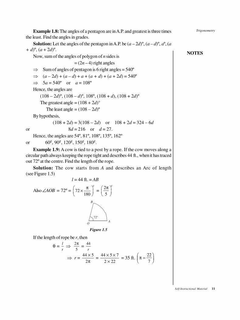
Example 1.9: A cow is tied to a post by a rope. If the cow moves along a
circular path always keeping the rope tight and describes 44 ft., when it has traced
out 72º at the centre. Find the length of the rope.
Solution: The cow starts from A and describes an Arc of length
(see Figure 1.5)
l = 44 ft. = AB
Also ∠AOB = 72º = 72180
cπ
×
= 2
5
cπ
OA
72°
B
Figure 1.5
If the length of rope be r, then
θ = l
r⇒
2
5
π =
44
r
⇒ r = 44 5
2
×
π =
44 5 7
2 22
× ×
× = 35 ft. π =
FHG
IKJ
22
7
12 Self-Instructional Material
Trigonometry
NOTES
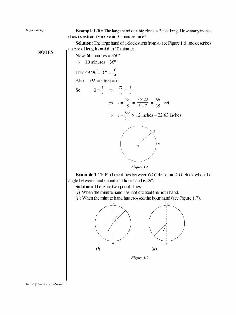
Example 1.10: The large hand of a big clock is 3 feet long. How many inches
does its extremity move in 10 minutes time?
Solution: The large hand of a clock starts from A (see Figure 1.6) and describes
an Arc of length l = AB in 10 minutes.
Now, 60 minutes = 360º
⇒ 10 minutes = 36º
Thus∠AOB =36º = 5
cπ
Also OA =3 feet = r
So θ =l
r⇒
π
5 =
3
l
⇒ l = 3
5
π =
3 22
5 7
×
× =
66
35 feet
⇒ l = 66
35 × 12 inches = 22.63 inches.
OB
A
Figure 1.6
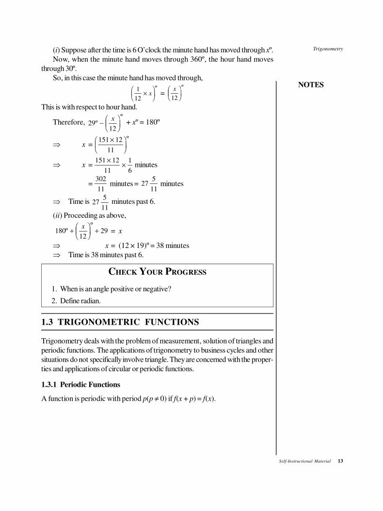
Example 1.11: Find the times between 6 O’clock and 7 O’clock when the
angle betwen minute hand and hour hand is 29º.
Solution: There are two possibilities:
(i) When the minute hand has not crossed the hour hand.
(ii) When the minute hand has crossed the hour hand (see Figure 1.7).12
6
x
12
6
(i) (ii)
Figure 1.7
Trigonometry
NOTES
Self-Instructional Material 13
(i) Suppose after the time is 6 O’clock the minute hand has moved through xº.
Now, when the minute hand moves through 360º, the hour hand moves
through 30º.
So, in this case the minute hand has moved through,
1
12×
FHGIKJx
º =
x
12
FHGIKJº
This is with respect to hour hand.
Therefore, 2912
ºº
−FHGIKJ
x + xº = 180º
⇒ x =151 12
11
×FHG
IKJº
⇒ x =151 12
11
1
6
×× minutes
=302
11 minutes = 27
5
11 minutes
⇒ Time is 275
11 minutes past 6.
(ii) Proceeding as above,
18012
29ºº
+FHGIKJ +
x= x
⇒ x = (12 × 19)º = 38 minutes
⇒ Time is 38 minutes past 6.
CHECK YOUR PROGRESS
1. When is an angle positive or negative?
2. Define radian.
1.3 TRIGONOMETRIC FUNCTIONS
Trigonometry deals with the problem of measurement, solution of triangles and
periodic functions. The applications of trigonometry to business cycles and other
situations do not specifically involve triangle. They are concerned with the proper-
ties and applications of circular or periodic functions.
1.3.1 Periodic Functions
A function is periodic with period p(p ≠ 0) if f(x + p) = f(x).
14 Self-Instructional Material
Trigonometry
NOTES
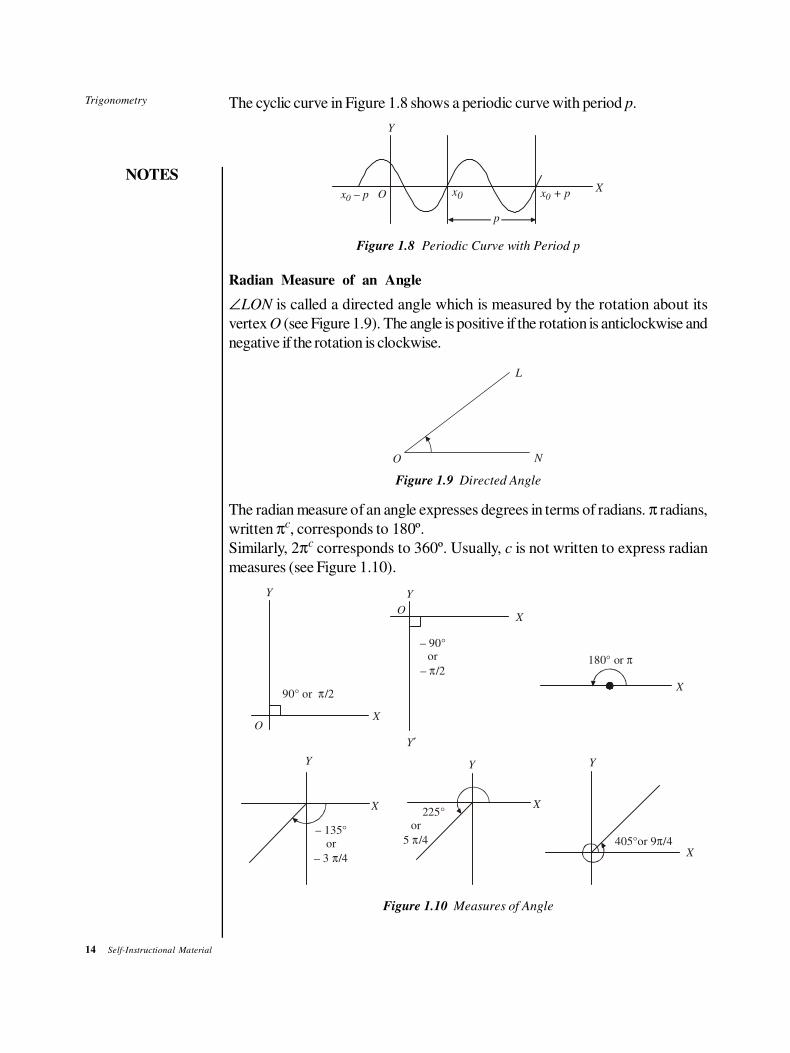
The cyclic curve in Figure 1.8 shows a periodic curve with period p.
Y
x – 0 p O x0 x + 0 p
p
X
Figure 1.8 Periodic Curve with Period p
Radian Measure of an Angle
∠LON is called a directed angle which is measured by the rotation about its
vertex O (see Figure 1.9). The angle is positive if the rotation is anticlockwise and
negative if the rotation is clockwise.
L
NO
Figure 1.9 Directed Angle
The radian measure of an angle expresses degrees in terms of radians. π radians,
written πc, corresponds to 180º.
Similarly, 2πc corresponds to 360º. Usually, c is not written to express radian
measures (see Figure 1.10).
X
Y
O
– 90°or
– π/2
Y′
Y
XO
90° or π/2
180° or π
X
Y
X
– 135°
or
– 3 π/4
Y
X 225°
or
5 π/4
Y
X
405°or 9 /4π
Figure 1.10 Measures of Angle
Trigonometry
NOTES
Self-Instructional Material 15
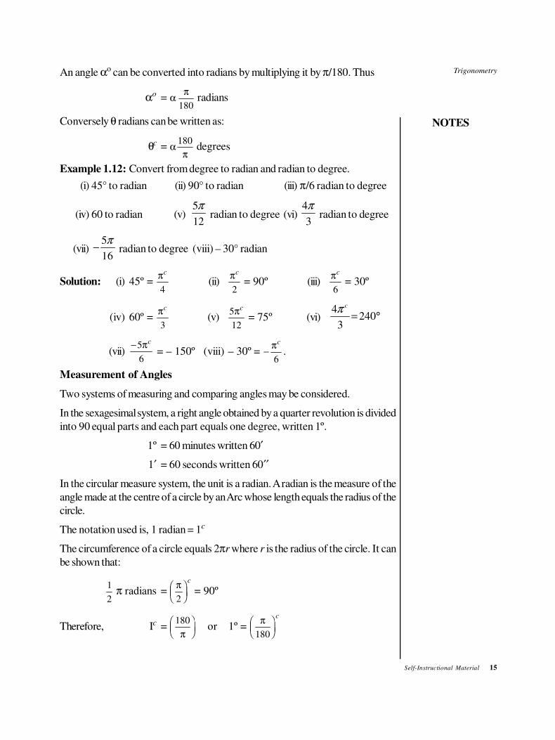
An angle αo can be converted into radians by multiplying it by π/180. Thus
αo = απ
180 radians
Conversely θ radians can be written as:
θc = απ
180 degrees
Example 1.12: Convert from degree to radian and radian to degree.
(i) 45° to radian (ii) 90° to radian (iii) π/6 radian to degree
(iv) 60 to radian (v) 5
12
π radian to degree (vi)
4
3
π radian to degree
(vii)5
16
π− radian to degree (viii) – 30° radian
Solution: (i) 45º = πc
4(ii)
πc
2 = 90º (iii)
πc
6 = 30º
(iv) 60º = πc
3(v)
5
12
πc
= 75º (vi)4
2403
cπ= °
(vii)−5
6
πc
= – 150º (viii) – 30º = −πc
6.
Measurement of Angles
Two systems of measuring and comparing angles may be considered.
In the sexagesimal system, a right angle obtained by a quarter revolution is divided
into 90 equal parts and each part equals one degree, written 1º.
1º = 60 minutes written 60′
1′ = 60 seconds written 60′′
In the circular measure system, the unit is a radian. A radian is the measure of the
angle made at the centre of a circle by an Arc whose length equals the radius of the
circle.
The notation used is, 1 radian = 1c
The circumference of a circle equals 2πr where r is the radius of the circle. It can
be shown that:
1
2 π radians =
π
2
FHGIKJ
c
= 90º
Therefore, Ic =180
π
FHGIKJ or 1º =
π
180
FHGIKJ
c
16 Self-Instructional Material
Trigonometry
NOTES
Since 1c is calculated by taking π = 3.141593 and it comes to 57.2958 and thus,
1c = 57º 17′ 45′′
Normally, approximate value of π is taken as, π = 22
7 or 3.142, 180º
= π radians, 360º = 2π radians
π
10 radians = 18º,
π
6 radians = 30º
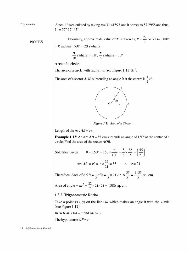
Area of a circle
The area of a circle with radius r is (see Figure 1.11) πr2.
The area of a sector AOB subtending an angle θ at the centre is 1
2
2r θ.
B
ArO
r
θ
Figure 1.11 Area of a Circle
Length of the Arc AB = rθ.
Example 1.13: An Arc AB = 55 cm subtends an angle of 150º at the centre of a
circle. Find the area of the sector AOB.
Solution: Given θ = 150º = 150180
×π
= 5
6
22
7× =
55
21
FHGIKJ
c
Arc AB = rθ = r ×55
21 = 55 ∴ r = 21
Therefore, Area of AOB = 1
2
2r θ =
1
221 21
55
21× × × =
1155
2 sq. cm.
Area of circle = πr2 =
22
721 21× × = 1386 sq. cm.
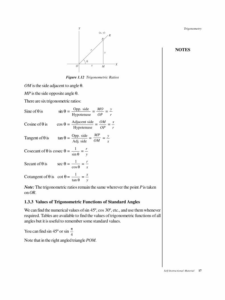
1.3.2 Trigonometric Ratios
Take a point P(x, y) on the line OR which makes an angle θ with the x-axis
(see Figure 1.12).
In ∆OPM, OM = x and MP = y
The hypotenuse OP = r
Trigonometry
NOTES
Self-Instructional Material 17
Y
X
y
Mx
r
P
R
O
( )x, y
Figure 1.12 Trigonometric Ratios
OM is the side adjacent to angle θ.
MP is the side opposite angle θ.
There are six trigonometric ratios:
Sine of θ is sin θ =Opp. side
Hypotenuse =
MO
OP =
y
r
Cosine of θ is cos θ =Adjacent side
Hypotenuse =
OM
OP =
x
r
Tangent of θ is tan θ =Opp. side
Adj. side =
MP
OM =
y
x
Cosecant of θ is cosec θ =1
sin θ =
r
y
Secant of θ is sec θ =1
cos θ =
r
x
Cotangent of θ is cot θ =1
tan θ =
x
y
Note: The trigonometric ratios remain the same wherever the point P is taken
on OR.
1.3.3 Values of Trigonometric Functions of Standard Angles
We can find the numerical values of sin 45º, cos 30º, etc., and use them whenever
required. Tables are available to find the values of trigonometric functions of all
angles but it is useful to remember some standard values.
You can find sin 45º or sinπ
4
Note that in the right angled triangle POM.
18 Self-Instructional Material
Trigonometry
NOTES
P
O M
a x
45
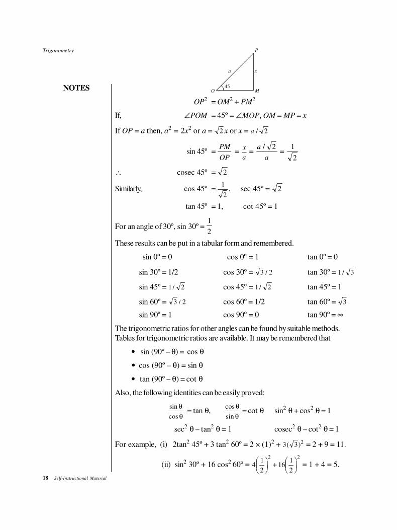
OP2 = OM
2 + PM2
If, ∠POM = 45º = ∠MOP, OM = MP = x
If OP = a then, a2 = 2x
2 or a = 2 x or x = a / 2
sin 45º =PM
OP =
x
a =
a
a
/ 2 =
1
2
∴ cosec 45º = 2
Similarly, cos 45º =1
2, sec 45º = 2
tan 45º = 1, cot 45º = 1
For an angle of 30º, sin 30º = 1
2
These results can be put in a tabular form and remembered.
sin 0º = 0 cos 0º = 1 tan 0º = 0
sin 30º = 1/2 cos 30º = 3 2/ tan 30º = 1 3/
sin 45º = 1 2/ cos 45º = 1 2/ tan 45º = 1
sin 60º = 3 2/ cos 60º = 1/2 tan 60º = 3
sin 90º = 1 cos 90º = 0 tan 90º = ∞
The trigonometric ratios for other angles can be found by suitable methods.
Tables for trigonometric ratios are available. It may be remembered that
• sin (90º – θ) = cos θ
• cos (90º – θ) = sin θ
• tan (90º – θ) = cot θ
Also, the following identities can be easily proved:
sin
cos
θ
θ= tan θ,
cos
sin
θ
θ = cot θ sin2 θ + cos2 θ = 1
sec2 θ – tan2 θ = 1 cosec2 θ – cot2 θ = 1
For example, (i) 2tan2 45º + 3 tan2 60º = 2 × (1)2 + 3 3 2( ) = 2 + 9 = 11.
(ii) sin2 30º + 16 cos2 60º = 41
216
1
2
2 2FHGIKJ +FHGIKJ = 1 + 4 = 5.
Trigonometry
NOTES
Self-Instructional Material 19
(iii) 4cos3 30º – 3cos 30º = 0 and
tan 45º – 2sin2 30º – cos 60º = 0
The trigonometric ratios are useful in finding the angles and lengths of the sides
of a triangle and for a variety of other purposes.
1.3.4 Signs of Trigonometric Ratios
As θ increases from 0 to 2π,
sin θ rises from 0 to 1 in Quadrant I (Q. I)
falls from 1 to 0 in Quadrant II (Q. II)
falls from 0 to – 1 in Quadrant III (Q. III)
rises from – 1 to 0 in Quadrant IV (Q. IV)
Similarly, cos θ falls from 1 to 0 in Q. I
falls from 0 to – 1 in Q. II
rises from – 1 to 0 in Q. III
rises from 0 to 1 in Q. IV
tan θ rises from 0 to ∞ in Q. I
rises from – ∞ to 0 in Q. II
rises from 0 to ∞ in Q. III
rises from – ∞ to 0 in Q. IV
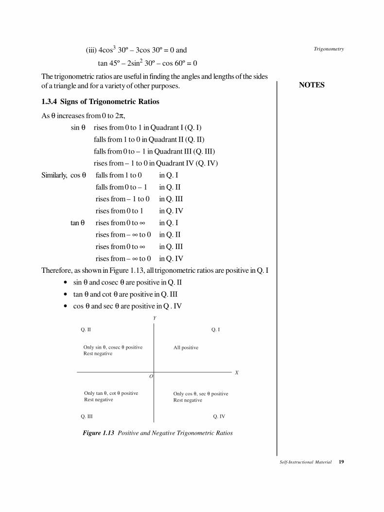
Therefore, as shown in Figure 1.13, all trigonometric ratios are positive in Q. I
• sin θ and cosec θ are positive in Q. II
• tan θ and cot θ are positive in Q. III
• cos θ and sec θ are positive in Q . IV
Q. II
Only sin , cosec positive
Rest negative
θ θ
Q. I
All positive
Only tan , cot positive
Rest negative
θ θ
Q. III
Only cos , sec positive
Rest negative
θ θ
Q. IV
OX
Y
Figure 1.13 Positive and Negative Trigonometric Ratios
20 Self-Instructional Material
Trigonometry
NOTES
The following results can be verified and used when required:
sin (– θ) = – sin θ
cos (– θ) = cos θ
tan (– θ) = –tan θ
The angle – θ is in the fourth quadrant in which cos (– θ) and Sec(–θ) are positive.
sin (90 – θ) = cos θ The angle 90 – θ is in the first quadrant. All ratios
cos (90 – θ) = sin θ are positive.
tan (90 – θ) = cot θ
sin (90 + θ) = cos θ The angle 90 + θ is in the second quadrant. Only
cos (90 + θ) = – sin θ sin (90 + θ) is positive.
tan (90 + θ) = – cot θ
sin (180 – θ) = sin θ The angle 180 – θ is in the second quadrant. Only
cos (180 – θ) = – cos θ sin (180 – θ) is positive.
tan (180 – θ) = – tan θ
sin (180 + θ) = – sin θ The angle 180 + θ is in the third quadrant. Only
cos (180 + θ) = – cos θ tan (180 + θ) is positive.
tan (180 + θ) = + tan θ
sin (360 – θ) = – sin θ Same rule as for the angle, – θ.
cos (360 – θ) = cos θ
tan (360 – θ) = – tan θ
sin (360 + θ) = sin θ
cos (360 + θ) = cos θ Same rule as for the angle θ.
tan (360 + θ) = tan θ
Ratios of other angles can be expressed in terms of the above ratios.
sin 32
πθ−
FHG
IKJ = sin (270 – θ) = sin (90 + 180 – θ)
= cos (180 – θ) = – cos θ
or sin (270 – θ) = sin (180 + 90 – θ)
= – sin (90 – θ) = – cos θ
or sin (270 – θ) = sin (270 – θ – 360)
= sin (– 90 – θ) = sin {– (90 + θ)} = – sin (90 + θ)
= – cos θ
Trigonometry
NOTES
Self-Instructional Material 21
or sin (270 – θ) = – sin (θ – 270)
= – sin (θ – 270 + 360) = – sin (90 + θ) = – cos θ
or sin (270 – θ) = – cos [90 + (270 – θ)] = – cos (360 – θ) = – cos θ
sin3
2π = sin (π + π/2) = − sin
π
2 = – 1
cos5
4π = −
1
2, sin
5
4π = −
1
2
cos7
4π =
1
2, sin
7
4π = −
1
2
cos7
6π = −
3
2, sin
7
6π = −
1
2
cos11
6π =
3
2, sin
11
6π = −
1
2
cos2
3π = −
1
2sin
5
3π = −
3
2
cos −FHGIKJ
3
4π = −
1
2, sin −
FHGIKJ
4
3π =
3
2
If sin θ = −3
5, then cos θ =
4
5, tan θ = −
3
4
cosec θ = −5
3, sec θ =
5
4, cot θ = −
4
3
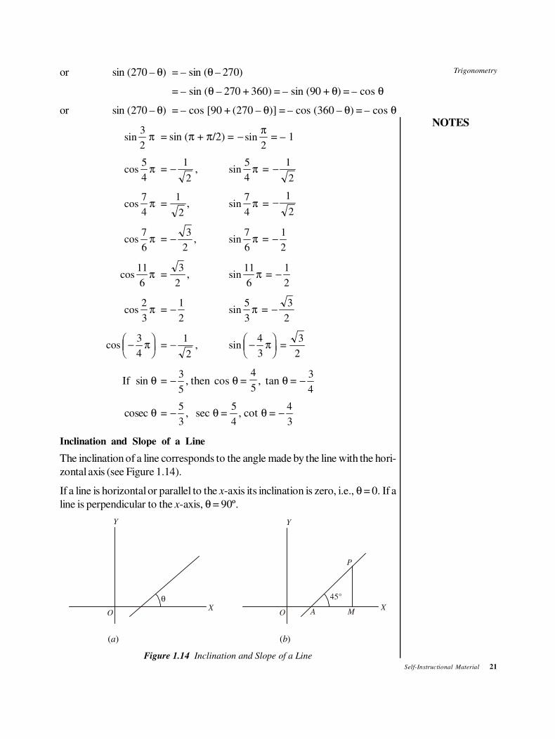
Inclination and Slope of a Line
The inclination of a line corresponds to the angle made by the line with the hori-
zontal axis (see Figure 1.14).
If a line is horizontal or parallel to the x-axis its inclination is zero, i.e., θ = 0. If a
line is perpendicular to the x-axis, θ = 90º.
Y
X
θ
O
Y
P
XMAO
45°
(a) (b)
Figure 1.14 Inclination and Slope of a Line
22 Self-Instructional Material
Trigonometry
NOTES
If the inclination of a line is θ, the slope of the line is tan θ.
The slope of a line with 45º inclination is tan 45º = 1. Alternatively, since ∠PAM
= 45º, AM = MP and tan 45º = MP/AM = 1.
For example the slope of a line with inclination (i) 30º (ii) 60º (iii) 0º (iv) 90º is
(i) tan 30º = 1
3(ii) tan 60º = 3 (iii) tan 0 = 0 (iv) tan 90º = ∞
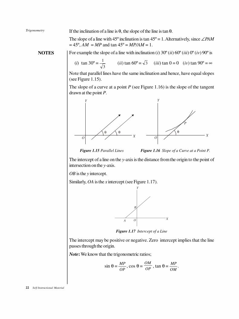
Note that parallel lines have the same inclination and hence, have equal slopes
(see Figure 1.15).
The slope of a curve at a point P (see Figure 1.16) is the slope of the tangent
drawn at the point P.
Y
OX
P
θ
Y
OX
θθ
Figure 1.15 Parallel Lines Figure 1.16 Slope of a Curve at a Point P.
The intercept of a line on the y-axis is the distance from the origin to the point of
intersection on the y-axis.
OB is the y intercept.
Similarly, OA is the x intercept (see Figure 1.17).
Y
OX
A
B
Figure 1.17 Intercept of a Line
The intercept may be positive or negative. Zero intercept implies that the line
passes through the origin.
Note: We know that the trigonometric ratios;
sin θ = MP
OP, cos θ =
OM
OP, tan θ =
MP
OM.
Trigonometry
NOTES
Self-Instructional Material 23
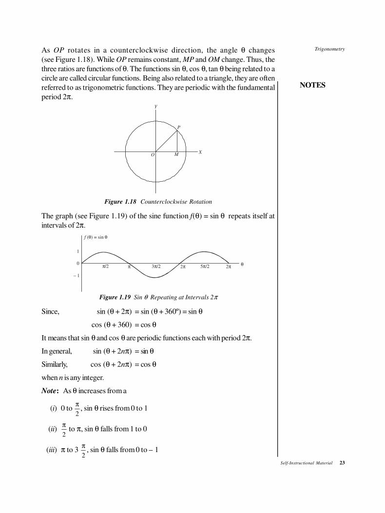
As OP rotates in a counterclockwise direction, the angle θ changes
(see Figure 1.18). While OP remains constant, MP and OM change. Thus, the
three ratios are functions of θ. The functions sin θ, cos θ, tan θ being related to a
circle are called circular functions. Being also related to a triangle, they are often
referred to as trigonometric functions. They are periodic with the fundamental
period 2π.
Y
P
XMO
Figure 1.18 Counterclockwise Rotation
The graph (see Figure 1.19) of the sine function f(θ) = sin θ repeats itself at
intervals of 2π.
f ( ) = sin θ θ
1
0
– 1
π/2 π 3 /2π 2π 5 /2π 2π θ
Figure 1.19 Sin θ Repeating at Intervals 2π
Since, sin (θ + 2π) = sin (θ + 360º) = sin θ
cos (θ + 360) = cos θ
It means that sin θ and cos θ are periodic functions each with period 2π.
In general, sin (θ + 2nπ) = sin θ
Similarly, cos (θ + 2nπ) = cos θ
when n is any integer.
Note: As θ increases from a
(i) 0 to π
2, sin θ rises from 0 to 1
(ii)π
2 to π, sin θ falls from 1 to 0
(iii) π to 3π
2, sin θ falls from 0 to – 1
24 Self-Instructional Material
Trigonometry
NOTES
(iv)3
2
π to 2π, sin θ rises from – 1 to 0
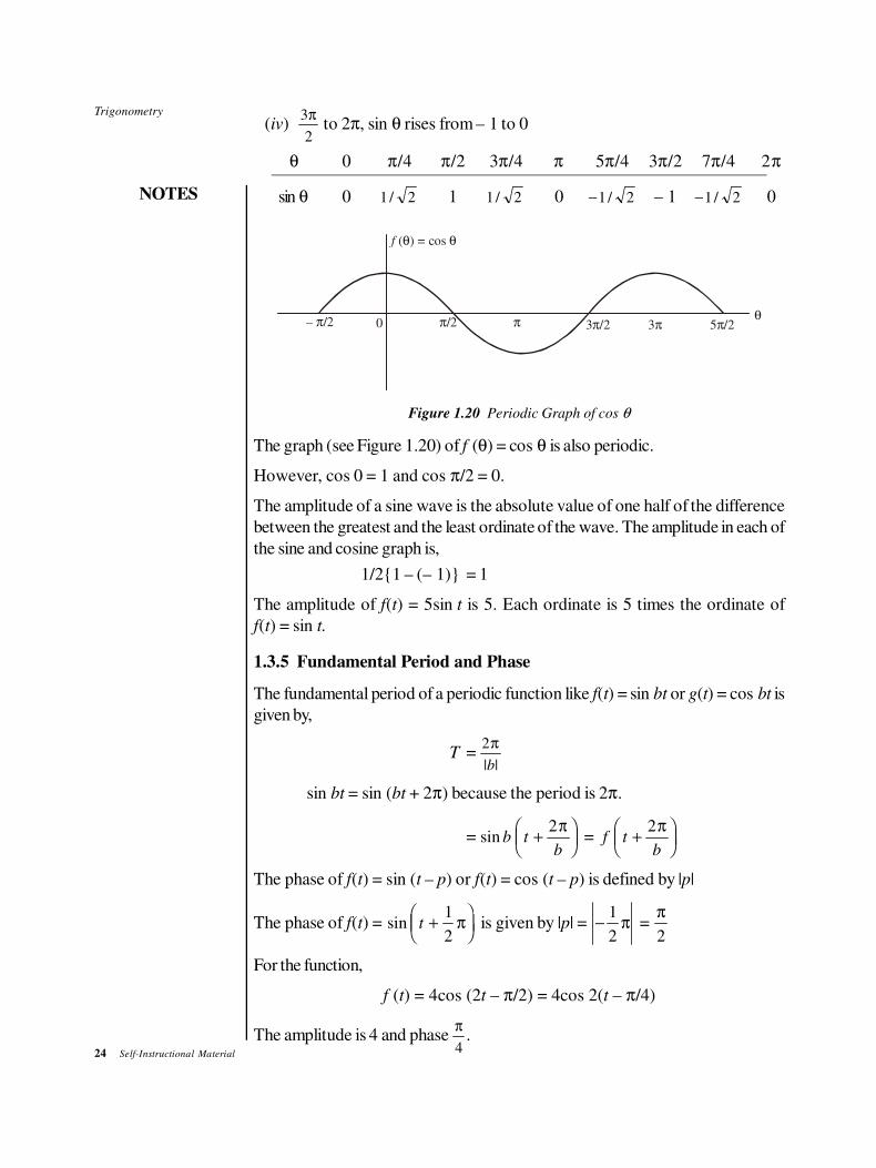
θ 0 π/4 π/2 3π/4 π 5π/4 3π/2 7π/4 2π
sin θ 0 1 2/ 1 1 2/ 0 −1 2/ – 1 −1 2/ 0
f ( ) = cos θ θ
– /2π 0 π/2 π 3 /2π 3π 5 /2πθ
Figure 1.20 Periodic Graph of cos θ
The graph (see Figure 1.20) of f (θ) = cos θ is also periodic.
However, cos 0 = 1 and cos π/2 = 0.
The amplitude of a sine wave is the absolute value of one half of the difference
between the greatest and the least ordinate of the wave. The amplitude in each of
the sine and cosine graph is,
1/2{1 – (– 1)} = 1
The amplitude of f(t) = 5sin t is 5. Each ordinate is 5 times the ordinate of
f(t) = sin t.
1.3.5 Fundamental Period and Phase
The fundamental period of a periodic function like f(t) = sin bt or g(t) = cos bt is
given by,
T =2π
| |b
sin bt = sin (bt + 2π) because the period is 2π.
= sin b tb
+FHG
IKJ
2π = f t
b+FHG
IKJ
2π
The phase of f(t) = sin (t – p) or f(t) = cos (t – p) is defined by |p|
The phase of f(t) = sin t +FHG
IKJ
1
2π is given by |p| = −
1
2π =
π
2
For the function,
f (t) = 4cos (2t – π/2) = 4cos 2(t – π/4)
The amplitude is 4 and phase π
4.
Trigonometry
NOTES
Self-Instructional Material 25
The fundamental period is 2
2
π = π.
The amplitude of 2 sin1
2π t is 2 and the fundamental period is
2
1 2
π
π( / ) = 4.
Example 1.14: If f(x) = sin kx is periodic, determine the period for f(x).
Solution: f (x) = sin (kx) = sin (kx + 2π) = sin k(x + 2π/k) = f (x + 2π/k)
The period is 2π/k.
This is also true for f(x) = cos kx. The period is 2π/k.
The period for f(x) = tan kx is π/k.
Example 1.15: Find the period, if any, for f(x) = sin x2.
Solution: If the period is t, f(x + t) = sin (x + t)2.
Also f(x) = sin x2 = sin (x2 + 2π)
∴ (x + t)2 = x2 + 2π
∴ 2tx + t2 = 2π which does not give a fixed value of t.
f(x) = sin x2
This function is not periodic.
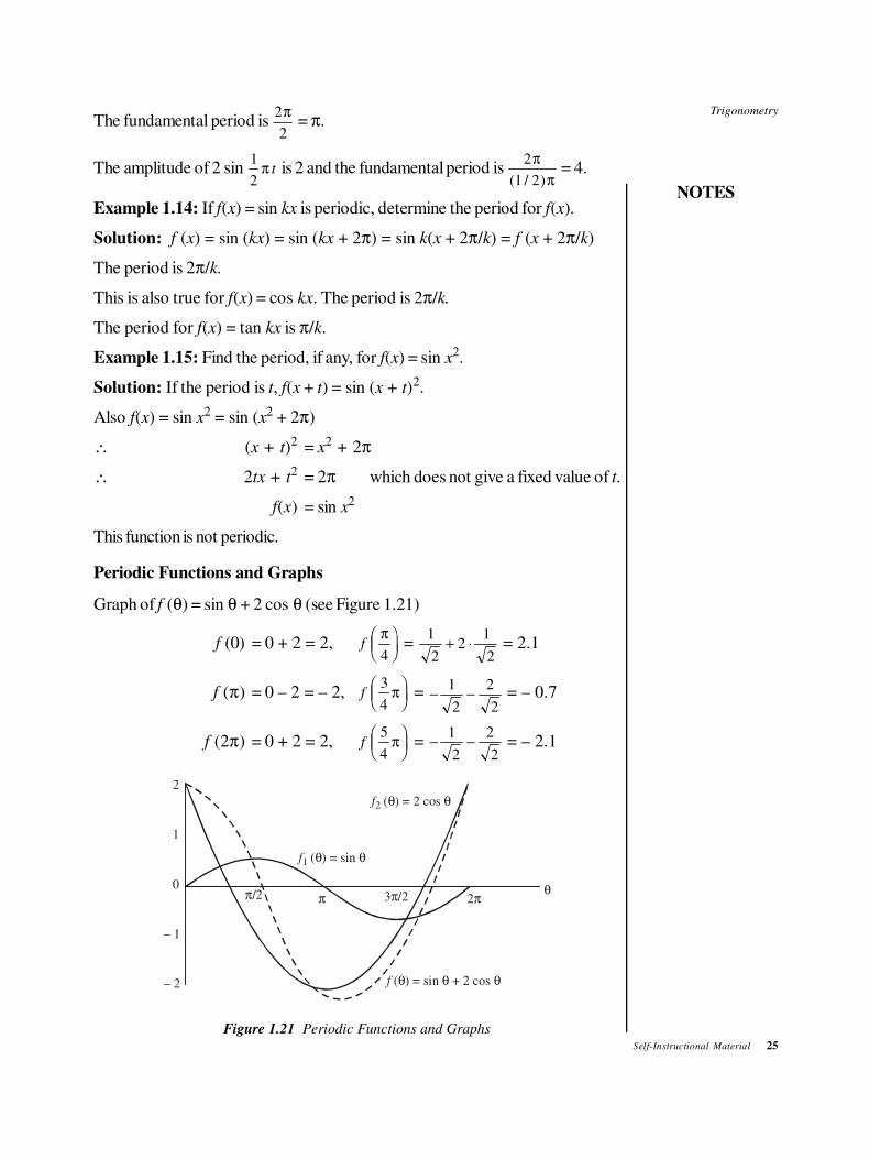
Periodic Functions and Graphs
Graph of f (θ) = sin θ + 2 cos θ (see Figure 1.21)
f (0) = 0 + 2 = 2, fπ
4
FHGIKJ =
1
22
1
2+ ⋅ = 2.1
f (π) = 0 – 2 = – 2, f3
4πFHGIKJ = − −
1
2
2
2 = – 0.7
f (2π) = 0 + 2 = 2, f5
4πFHGIKJ = − −
1
2
2
2 = – 2.1
f2 ( ) = 2 cos θ θ
f1 ( ) = sin θ θ
2
1
0
– 1
– 2 f ( ) = sin + 2 cosθ θ θ
2π ππ/2 3 /2πθ
Figure 1.21 Periodic Functions and Graphs
26 Self-Instructional Material
Trigonometry
NOTES
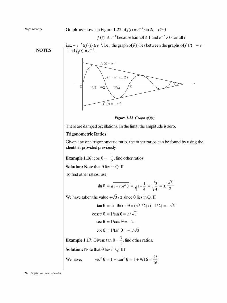
Graph as shown in Figure 1.22 of f(t) = e– t sin 2t t ≥ 0
|f (t)| ≤ e– t because |sin 2t| ≤ 1 and e– t > 0 for all t
i.e., – e– t ≤ f (t) ≤ e– t, i.e., the graph of f(t) lies between the graphs of f
1(t) = – e
–
t and f2(t) = e– t.
f t = e2 ( ) –t
f t e t ( ) = sin 2 –t
O π/4 π/2 3 /4π π
f t = – e1 ( ) –t
t
Figure 1.22 Graph of f(t)
There are damped oscillations. In the limit, the amplitude is zero.
Trigonometric Ratios
Given any one trigonometric ratio, the other ratios can be found by using the
identities provided previously.
Example 1.16: cos θ = −1
2, find other ratios.
Solution: Note that θ lies in Q. II
To find other ratios, use
sin θ = 1 2− cos θ = 11
4− =
3
4 = ±
3
2
We have taken the value + 3 2/ since θ lies in Q. II
tan θ = sin θ/cos θ = ( / ) / ( / )3 2 1 2− = − 3
cosec θ = 1/sin θ = 2 3/
sec θ = 1/cos θ = – 2
cot θ = 1/tan θ = −1 3/
Example 1.17: Given: tan θ = 3
4, find other ratios.
Solution: Note that θ lies in Q. III
We have, sec2 θ = 1 + tan2 θ = 1 + 9/16 = 25
16
Trigonometry
NOTES
Self-Instructional Material 27
sec θ = ± 5
4
sec θ = −5
4 since θ lies in Q. III
cos θ = – 4/5
sin θ = 1 2− cos θ = 116
25− =
9
25 = −
3
5 (Q. III)
cot θ = 4/3, cosec θ = – 5/3.
Exmaple 1.18: Show 4cot2 45º – sec2 60º + sin2 30º = 1
4.
Solution: 4 × (1)2 – (2)2 +
21
2
= 4 – 4 + 1 1
4 4=
Identities
In the forthcoming exercises, the following identities will be useful.
(i) sin2A + cos2
A = 1, (ii) sec2A = 1 + tan2
A, (iii) cosec2A = 1 + cot2
A
Example 1.19: Prove that: 1
1
−
+
sin
sin
A
A = sec A – tan A
Solution: LHS =( sin )( sin )
( sin )( sin )
1 1
1 1
− −
+ −
A A
A A =
( sin )
sin
1
1
2
2
−
−
A
A
=( sin )
cos
1 2
2
− A
A =
1 − sin
cos
A
A =
1
cos
sin
cosA
A
A−
= sec A – tan A
Example 1.20: Prove that cos
tan
sin
cot
A
A
A
A1 1−+
− = sin A + cos A.
Solution: Put tan A = sin A/cos A and cot A = cos A/sin A
LHS =cos cos
cos sin
sin sin
sin cos
A A
A A
A A
A A
⋅
−+
− =
cos
cos sin
sin
cos sin
2 2A
A A
A
A A−−
−
=cos sin
cos sin
2 2A A
A A
−
− =
(cos sin )(cos sin )
cos sin
A A A A
A A
+ −
− = cos A + sin A.
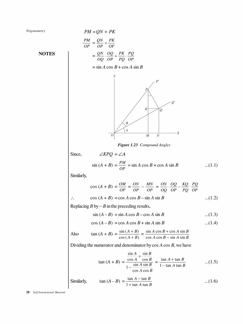
Compound Angles
To find sin (A + B).
From a point P on OP′ draw PQ ⊥ OQ′ (see Figure 1.23).
From Q draw QK ⊥ PM.
28 Self-Instructional Material
Trigonometry
NOTES
PM =QN + PK
PM
OP=
QN
OP
PK
OP+
= QN
OQ
OQ
OP
PK
PQ
PQ
OP⋅ + ⋅
= sin A cos B + cos A sin B
Y
O M NX
A
B
P′
P
K Q
Q′
Figure 1.23 Compound Angles
Since, ∠KPQ = ∠Α
sin (A + B) =PM
OP = sin A cos B + cos A sin B ...(1.1)
Similarly,
cos (A + B) =OM
OP =
ON
OP –
MN
OP =
ON
OQ
OQ
OP
KQ
PQ
PQ
OP⋅ − ⋅
∴ cos (A + B) = cos A cos B – sin A sin B ...(1.2)
Replacing B by – B in the preceding results,
sin (A – B) = sin A cos B – cos A sin B ...(1.3)
cos (A – B) = cos A cos B + sin A sin B ...(1.4)
Also tan (A + B) =sin ( )
cos ( )
A B
A B
+
+ =
sin cos cos sin
cos cos sin sin
A B A B
A B A B
+
−
Dividing the numerator and denominator by cos A cos B, we have
tan (A + B) =
sin
cos
sin
cos
sin sin
cos cos
A
A
B
B
A B
A B
+
−1
= tan tan
tan tan
A B
A B
+
−1...(1.5)
Similarly, tan (A – B) =tan tan
tan tan
A B
A B
−
+1...(1.6)
Trigonometry
NOTES
Self-Instructional Material 29
It can be seen by putting A + B = C, and A – B = D that
sin C + sin D = 22 2
sin cosC D C D+ −
;
sin C – sin D = 22 2
cos sinC D C D+ −
;
cos C + cos D = 22 2
cos cosC D C D+ −
;
cos C – cos D = −+ −
22 2
sin sinC D C D
.
We know that, sin (A + B) = sin A cos B + cos A sin B ...(1.7)
Put A = B, then sin (2A) = sin A cos A + cos A sin A
We have the result sin 2A = 2 sin A cos A ...(1.8)
On the same lines, using the result for cos (A + B) we can prove
cos 2A = cos2 – sin2A = 2 cos2
A – 1 = 1 – 2 sin2A ...(1.9)
sin 3A = sin (2A + A) = sin 2A cos A + cos 2A sin A
= 2 sin A cos A + (1 – 2 sin2A) sin A
= 2 sin A(1 – sin2A) + (1 – 2 sin2
A) sin A
= 2 sin A – 2 sin3A + sin A – 2 sin3
A
∴ sin 3A = 3 sin A – 4 sin3A ...(1.10)
Similarly, cos 3A = cos (2A + A) = 4 cos3A – 3 cos A ...(1.11)
tan 3A = tan (2A + A) = tan tan
tan tan
2
1 2
A A
A A
+
−
=
2
−+
−2
−
tan
tantan
tan
tantan
A
AA
A
AA
1
11
2
2
= 2 + −
− −
tan tan tan
tan tan
A A A
A A
3
2 21 2
= 3
1 3
3
2
tan tan
tan
A A
A
−
−...(1.12)
In the result cos 2A = cos2A – sin2
A, if we replace A by A
2 we have
cos A = cos sin2 2
2 2
A A− = 2
212cos
A− = 1 2
2
2− sinA
...(1.13)
Similarly, sin A = 22 2
sin cosA A
...(1.14)
30 Self-Instructional Material
Trigonometry
NOTES
tan A =2 2
1 22
tan /
tan /
A
A− =
2
1 2
t
t− where t = tan
A
2...(1.15)
The following additional results are useful and may be derived:
Since cos 2A = 2 cos2A – 1 = 1 – 2 sin2
A
∴ cos2A =
1 2
2
+ cos Aor cos A = ±
+1 2
2
cos A
sin2A =
1 2
2
− cos Aor sin A = ±
−1 2
2
cos A
Summary of Some Important Results
I. sin (A ± B) = sin A cos B ± cos A sin B
cos (A ± B) = cos A cos B ∓ sin A sin B
sin (A + B + C) = sin A cos B cos C + cos A sin B cos C
+ cos A cos B sin C – sin A sin B sin C
cos (A + B + C) = cos A cos B cos C – cos A sin B sin C – sin A cos B
sin C
– sin A sin B cos C
tan (A + B) =tan tan
tan tan
A B
A B
+
−1, tan (A – B) =
tan tan
tan tan
A B
A B
−
+1
tan (A + B + C) =tan tan tan tan tan tan
tan tan tan tan tan tan
A B C A B C
B C C A A B
+ + −
− − −1
cot (A + B) =cot cot
cot cot
A B
B A
−
+
1 cot (A – B) =
cot cot
cot cot
A B
B A
+
−
1
II. sin 2A = 2 sin A cos A = 2
1 2
tan
tan
A
A+ sin A =
2 2
1 22
tan /
tan /
A
A+
cos 2A =
= −
= −
= −
RS|
T|
UV|
W|
cos sin
sin
cos
2 2
2
2
1 2
2 1
A A
A
A
= 1
1
2
2
−
+
tan
tan
A
A; cos A =
1 2
1 2
2
2
−
+
tan /
tan /
A
A
tan 2A = 2
1 2
tan
tan
A
A− =
1
1
2
2
−
+
cos
cos
A
A; tan A =
2 2
1 22
tan /
tan /
A
A−
1 – cos 2A = 2 sin2A
1 + cos 2A = 2 cos2A
sin 3A = 3 sin A – 4 sin3A
cos 3A = 4 cos3A – 3 cos A
Trigonometry
NOTES
Self-Instructional Material 31
tan 3A =3
1 3
3
2
tan tan
tan
A A
A
−
−
III. Conversion of product into sum:
sin A cos B =1
2{sin ( ) sin ( )}A B A B+ + −
cos A sin B =1
2{sin ( ) sin ( )}A B A B+ − −
cos A cos B =1
2{cos ( ) cos ( )}A B A B+ + −
sin A sin B = − + − −1
2{cos ( ) cos ( )}A B A B
IV. Conversion of sum into product
sin C + sin D = 22 2
sin cosC D C D+ −
sin C – sin D = 22 2
cos sinC D C D+ −
cos C + cos D = 22 2
cos cosC D C D+ −
cos C – cos D = −+ −
22 2
sin sinC D C D
V. cos A/2 = ±+1
2
cos A...(1.16)
sin A/2 = ±−1
2
cos A...(1.17)
tan A/2 = ±−
+
1
1
cos
cos
A
A...(1.18)
Also, if we write tan A/2 = t, we have
sin A =2
1 2
t
t+, cos A =
1
1
2
2
−
+
t
t, tan A =
2
1 2
t
t−...(1.19)
tanA
2=
sin /
cos /
A
A
2
2 =
sin / cos /
cos / cos /
A A
A A
2 2 2
2 2 2
⋅
⋅
= sin
cos /
A
A2 22 =
sin
cos
A
A1 +.
32 Self-Instructional Material
Trigonometry
NOTES
Example 1.21: Prove: (i) tan2A cosec A =
sin
sin
A
A1 2−
(ii) sec
sin
2
2
1A
A
− =
12cos A
Solution: (i) sin
cos sin
A
A A
FHGIKJ
21
= sin
cos sin
2
2
1A
A A⋅ =
sin
cos
A
A2
= 2
sin
1 sin
A
A−
(ii) sec
sin
2
2
1A
A
− =
tan
sin
2
2
A
A =
sin
cos sin
2
⋅A
A A2 2
1 =
12cos A
Example 1.22: Given q cos θ = p sin θ, find the value of p q
p q
cos sin
cos sin
θ θ
θ θ
+
−.
Solution: Since q cos θ = p sin θ cos θ p
q sin θ and hence, p cos θ =
p
q
2
sin θ ,
the expression becomes
p
p
2
2
sin sin
sin sin
θ θ
θ θ
+
−
=
p
p
2
2
+FHG
IKJ
−FHG
IKJ
sin
sin
θ
θ
= p q
p q
2 2
2 2
+
−.
Example 1.23: Prove that sin (A + B) sin (A – B) = sin2A – sin2
B.
Solution: LHS = (sin A cos B + cos A sin B)(sin A cos B – cos A sin B)
= sin2A cos2
B – cos2A sin2
B
= sin2A (1 – sin2
B) – (1 – sin2A) sin2
B
= sin2A – sin2
A sin2B – sin2
B + sin2A sin2
B = sin2A –sin2
B.
Example 1.24: Prove that cos º sin º
cos º sin º
9 9
9 9
+
− = tan 54º.
Solution: Divide Numerator and Denominator by cos 9º
LHS =1 9
1 9
+
−
tan º
tan º =
tan º tan º
tan º tan º
45 9
1 45 9
+
−(∵ tan 45º = 1)
= tan (45º + 9º) = tan 54º
Example 1.25: Prove that 814
3
14
5
14sin sin sin
π π π = 1.
Solution: LHS = 82 14 2
3
14 2
5
14cos cos cos
π π π π π π−FHG
IKJ −FHG
IKJ −FHG
IKJ
=83
7
2
7 7cos cos cos
π π π =
8
27
27 7
2
7
3
7sin
sin cos cos cosπ
π π π π⋅
[2 sin A cos A = sin 2A]
Trigonometry
NOTES
Self-Instructional Material 33
=8
2 7
2
7
2
7 7sin /sin cos cos
π
π π π3 =
8
47
4
7
3
7sin
sin cosπ
π π
=8
8 7 7sin /sin sin
ππ
π+
FHG
IKJ =
1
70 7
sin /( sin / )
ππ+ = 1.
Example 1.26: If A + B + C = π, show that:
cos 2A + cos 2B + cos 2C = – 1 – 4 cos A cos B cos C
Solution: LHS = (2 cos2A – 1) + 2 cos (B + C) cos (B – C)
Since B + C = π – A, cos (B + C) = cos (π – A) = – cos A
LHS = – 1 + 2 cos2A – 2 cos A cos (B – C)
= – 1 + 2 cos A (cos A – cos (B – C))
= – 1 – 2 cos A (– cos (B + C) – cos (B – C))
= – 1 – 2 cos A 2 cos B cos C
= – 1 – 4 cos A cos B cos C.
Example 1.27: If cos θ + sin θ = 2 cos θ, show cos θ – sin θ = 2 sin θ.
Solution: Dividing by cos θ, we have
1 + tan θ = 2 or tan θ = 2 – 1 < 1, i.e., sin θ < cos θ
Squaring, cos θ + sin θ = 2 cos θ
cos2 θ + sin2 θ + 2 cos θ sin θ = 2 cos2 θ
∴ cos2 θ – sin2 θ – 2 cos θ sin θ = 0
∴ (cos θ – sin θ)2 = 2 sin2 θ
∴ cos θ – sin θ = ± 2 sin θ
∴ cos θ – sin θ = 2 sin θ
(– 2 sin θ not possible because tan θ < 1)
Example 1.28: Given a = sin A + sin B, b = cos A + cos B, show that:
tan A B−
2 =
4 2 2
2 2
− −
+
a b
a b.
Solution: We have:
a2 + b2 = (sin A + sin B)2 + (cos A + cos B)2
= sin2A + 2 sin A sin B + sin2
B + cos2A + 2 cos A cos B +
cos2B
34 Self-Instructional Material
Trigonometry
NOTES
= 1 + 2 (sin A sin B + cos A cos B) + 1 = 2 + 2 cos (A – B)
4 2 2
2 2
− −
+
a b
a b=
41
2 2a b+
− = 4
2 11
( cos ( ))+ −−
A B
=1
1
− −
+ −
cos ( )
cos ( )
A B
A B =
22
22
2
2
sin
cos
A B
A B
−
− = tan2
2
A B−
∴4 2 2
2 2
− −
+
a b
a b= tan
A B−
2
Example 1.29: Show cos cos
sin sin
sin sin
cos cos
A B
A B
A B
A B
n n
+
−
FHG
IKJ +
+
−
FHG
IKJ = 2
2cotn A B−
or 0.
Solution: LHS = 2
2 2
22 2
22 2
22 2
cos cos
cos sin
cos cos
sin sin
A B A B
A B A B
A B A B
A B A B
n n+ −
+ −
F
HGGG
I
KJJJ
+
+ −
−+ −
F
HGGG
I
KJJJ
= 22
cotn A B−if n is even
= 0 if n is odd.
CHECK YOUR PROGRESS
3. State the formula for the area of a circle.
4. What is the formula for the area of a sector of a circle?
5. What is the measure of inclination in the following cases:
(i) A line is either horizontal or parallel to the x-axis?
(ii) A line is perpendicular to the x-axis?
6. What is the fundamental period of a periodic function like f(t) = sin bt or
g(t) = cos bt?
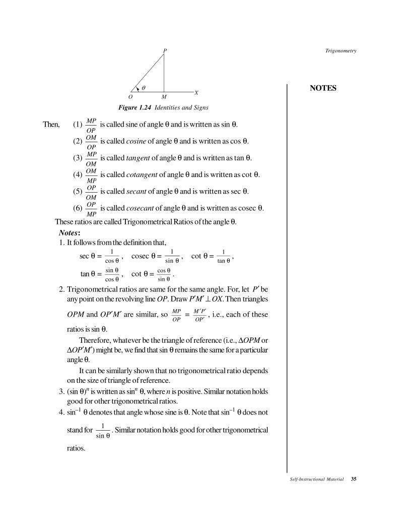
1.4 IDENTITIES AND SIGNS
Let a revolving line OP start from OX in the anticlockwise direction and trace out
an angle XOP. From P draw PM ⊥ OX. Produce OX, if necessary. (see Figure
1.24). Let ∠XOP = θ.
Trigonometry
NOTES
Self-Instructional Material 35
q
O MX
P
Figure 1.24 Identities and Signs
Then, (1) MP
OP is called sine of angle θ and is written as sin θ.
(2) OM
OP is called cosine of angle θ and is written as cos θ.
(3) MP
OM is called tangent of angle θ and is written as tan θ.
(4) OM
MP is called cotangent of angle θ and is written as cot θ.
(5) OP
OM is called secant of angle θ and is written as sec θ.
(6) OP
MP is called cosecant of angle θ and is written as cosec θ.
These ratios are called Trigonometrical Ratios of the angle θ.
Notes:
1. It follows from the definition that,
sec θ = 1
cos θ, cosec θ =
1
sin θ, cot θ =
1
tan θ,
tan θ = sin
cos
θ
θ, cot θ =
cos
sin
θ
θ.
2. Trigonometrical ratios are same for the same angle. For, let P′ be
any point on the revolving line OP. Draw P′M′ ⊥ OX. Then triangles
OPM and OP′M′ are similar, so MP
OP =
M P
OP
′ ′
′, i.e., each of these
ratios is sin θ.
Therefore, whatever be the triangle of reference (i.e., ∆OPM or
∆OP′M′) might be, we find that sin θ remains the same for a particular
angle θ.
It can be similarly shown that no trigonometrical ratio depends
on the size of triangle of reference.
3. (sin θ)n is written as sinn θ, where n is positive. Similar notation holds
good for other trigonometrical ratios.
4. sin–1 θ denotes that angle whose sine is θ. Note that sin–1 θ does not
stand for 1
sin θ. Similar notation holds good for other trigonometrical
ratios.
36 Self-Instructional Material
Trigonometry
NOTES
For any Angle θθθθ,
1. sin2 θ + cos2 θ = 1
2. sec2 θ = 1 + tan2 θ
3. cosec2 θ = 1 + cot2 θ
Proof: Let the revolving line OP start from OX and trace out an angle θ in the
anticlockwise direction. From P draw PM ⊥ OX. Produce OX, if necessary.
Then, ∠XOP = θ.
(1) sin θ = MP
OP, cos θ =
OM
OP
Then, sin2 θ + cos2 θ = ( ) ( )
( )
MP OM
OP
2 2
2
+ =
( )
( )
OP
OP
2
2 = 1.
(2) sec θ = OP
OM, tan θ =
MP
OM
Then, 1 + tan2 θ = 12
2+
( )
( )
MP
OM
= ( ) ( )
( )
OM MP
OM
2 2
2
+
= ( )
( )
OP
OM
2
2 =
OP
OM
FHGIKJ
2
= (sec θ)2 = sec2 θ
(3) cot θ = OM
MP, cosec θ =
OP
MP.
Then, 1 + cot2 θ = 1
2
+FHGIKJ
OM
MP =
( ) ( )
( )
MP OM
MP
2 2
2
+
=( )
( )
OP
MP
2
2 =
OP
MP
FHGIKJ
2
= (cosec θ)2 = cosec2 θ.
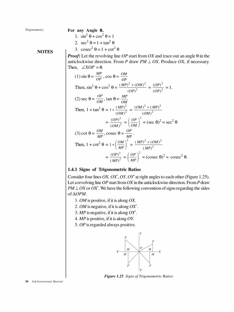
1.4.1 Signs of Trigonometric Ratios
Consider four lines OX, OX′, OY, OY′ at right angles to each other (Figure 1.25).
Let a revolving line OP start from OX in the anticlockwise direction. From P draw
PM ⊥ OX or OX′. We have the following convention of signs regarding the sides
of ∆OPM.
1. OM is positive, if it is along OX.
2. OM is negative, if it is along OX′.
3. MP is negative, if it is along OY′.
4. MP is positive, if it is along OY.
5. OP is regarded always positive.
X' X
Y
Y'
PP
M M
MM
O
P
P
Figure 1.25 Signs of Trigonometric Ratios
Trigonometry
NOTES
Self-Instructional Material 37
First quadrant. If the revolving line OP is in the first quadrant, then all the sides of
the triangle OPM are positive. Therefore, all the trigonometric ratios are positive
in the first quadrant.
Second quadrant. If the revolving line OP is in the second quadrant, then OM is
negative and the other two sides of ∆OPM are positive. Therefore, ratios involving
OM will be negative. So, cosine, secant, tangent, cotangent of an angle in the
second quadrant are negative while sine and cosecant of anlge in the second quadrant
are positive.
Third quadrant. If the revolving line is in the third quadrant, then sides OM and
MP both are negative. Since OP is always positive, therefore, ratios involving
each one of OM and MP alone will be negative. So, sine, cosine, cosecant and
secant of an angle in the third quadrant are negative. Since tangent or cotangent of
any angle involve both OM and MP, therefore, these will be positive. So, tangent
and cotangent of an angle in the third quadrant are positive.
Fourth quadrant. If the revolving line OP is in the fourth quadrant, then MP is
negative and the other two sides of ∆OPM are positive. Therefore, ratios involving
MP will be negative and others positive. So, sine, cosecant, tangent and cotangent
of an angle in the fourth quadrant are negative while cosine and secant of an angle
in the fourth quadrant are positive.
Limits to the Value of Trigonometric Ratios
We know that sin2 θ + cos2 θ = 1 for any angle θ. sin2 θ and cos2 θ being perfect
squares, will be positive. Again neither of them can be greater than 1 because then
the other will have to be negative.
Thus, sin2 θ ≤ 1, cos2 θ ≤ 1.
⇒ sin θ and cos θ cannot be numerically greater than 1.
Similarly, cosec θ =1
sin θ and sec θ =
1
cos θ cannot be numerically less
than 1.
There is no restriction on tan θ and cot θ. They can have any value.
Example 1.30: Prove that sin6 θ + cos6 θ = 1 – 3 sin2 θ cos2 θ.
Solution: Here LHS=sin6 θ + cos6 θ
=(sin2 θ)3 + (cos2 θ)3
=(sin2 θ + cos2 θ)(sin4 θ – sin2 θ cos2 θ + cos4 θ)
=1 . (sin4 θ – sin2 θ cos2 θ + cos4 θ)
=[(sin2 θ + cos2 θ)2 – 3 sin2 θ cos2 θ]
=1 – 3 sin2 θ cos2 θ = RHS.
Example 1.31: Prove that1 cos
1 cos
+
−
θ
θ= cosec θ + cot θ. Provided
cos θ ≠ 1.
38 Self-Instructional Material
Trigonometry
NOTES
Solution: LHS =1
1
+
−
cos
cos
θ
θ =
( cos )( cos )
( cos )( cos )
1 1
1 1
+ +
− +
θ θ
θ θ = −
+
−
1
12
cos
cos
θ
θ
=1 + cos
sin
θ
θ =
1
sin
cos
sinθ
θ
θ+ = cosec θ + cot θ.
Example 1.32: Prove that (1 + cot θ – cosec θ)(1 + tan θ + sec θ) = 2.
Solution: LHS = (1 + cot θ – cosec θ)(1 + tan θ + sec θ)
= 11
11
+ −FHG
IKJ + +FHG
IKJ
cos
sin sin
sin
cos cos
θ
θ θ
θ
θ θ
LHS = (sin cos )(cos sin )
sin cos
θ θ θ θ
θ θ
+ − + +1 1
= (sin cos )
sin cos
θ θ
θ θ
+ −21
= sin cos sin cos
sin cos
2 2 2 1θ θ θ θ
θ θ
+ + −
= 1 2 1+ −sin cos
sin cos
θ θ
θ θ =
2 sin cos
sin cos
θ θ
θ θ = 2 = RHS.
Example 1.33: Prove that tan θ cot θ
1– cot θ 1– tanθ+ = 1 + cosec θ sec θ, if
cot θ ≠ 1, 0 and tan θ ≠ 1, 0.
Solution: LHS =tan
cot
cot
tan
θ
θ
θ
θ1 1−+
−
=tan
tan
tan
tan
θ
θ
θ
θ1
1
1
1−
+−
=tan
tan tan ( tan )
2
1
1
1
θ
θ θ θ−+
−
=tan
tan tan (tan )
2
1
1
1
θ
θ θ θ−−
−
=tan
tan (tan )
31
1
θ
θ θ
−
−
=(tan )(tan tan )
tan (tan )
θ θ θ
θ θ
− + +
−
1 1
1
2
=tan tan
tan
21θ θ
θ
+ + since tan θ ≠ 1
=sec tan
tan
2 θ θ
θ
+
=sec
tan
2
1θ
θ+ = sec θ cosec θ + 1 = RHS.
Trigonometry
NOTES
Self-Instructional Material 39
Example 1.34: Which of the six trigonometrical ratios are positive for (i)
960º (ii) – 560º?
Solution: (i) 960º = 720º + 240º.
Therefore, the revolving line starting from OX will make two complete
revolutions in the anticlockwise direction and further trace out an angle of 240º in
the same direction. Thus, it will be in the third quadrant. So, the tangent and
cotangent are positive and rest of trigonometrical ratios will be negative.
(ii) – 560º = – 360º – 200º.
Therefore, the revolving line after making one complete revolution in the
clockwise direciton, will trace out further an angle of 200º in the same direction.
Thus, it will be in the second quadrant. So, only sine and cosecant are positive.
Example 1.35: In what quadrants can θ lie if sec θ = 7
6
−?
Solution: As sec θ is negative in second and third quadrants, θ can lie in
second or third quadrant only.
Example 1.36: If sin θ =12
13
−, determine other trigonometrical ratios
of θ.
Solution: cos2 θ = 1 – sin2 θ
= 1144
169− =
169 144
169
− =
25
169
⇒ cos θ = ±5
13
So tan θ =sin
cos
θ
θ = ∓
12
5
cosec θ =−13
12, sec θ = ±
13
5, cot θ = ∓
5
12.
Example 1.37: Express all the trigonometrical ratios of θ in terms of the sin θ.
Solution: Let sin θ = k.Then, cos2 θ = 1 – sin2 θ = 1 – k2
⇒ cos θ = ± −1 2k 21 sin θ± −
tan θ =sin
cos
θ
θ = ±
−
k
k1 2 = ±
2
sin θ
1– sin θ
cot θ =cos
sin
θ
θ = ±
−12
k
k = ±
21 sin θ
sinθ
−
sec θ =1
cos θ = ±
−
1
1 2k
= ± 2
1
1 sin θ−
cosec θ =1
sinθ =
1
k =
1
sin θ
40 Self-Instructional Material
Trigonometry
NOTES
Example 1.38: Prove that sin θ = a1
a+ is impossible, if a is real.
Solution: sin θ = aa
+1
⇒ sin θ = a
a
2 1+
⇒ a2 – a sin θ + 1 = 0
⇒ a = sin sinθ θ± −2 4
2For a to be real, the expression under the radical sign, must be positive or
zero.
i.e., sin2 θ – 4 ≥ 0
or sin2 θ ≥ 4 ⇒ sin θ is numerically greater than or
equal to 2 which is impossible.
Thus, if a is real, sin θ = aa
+1
is impossible.
Example 1.39: Prove that:
1 1 1 1
cosec θ cot θ sin θ sin θ cosec θ – cot θ− = −
+
Solution: LHS =1 1
cosec θ θ θ+−
cot sin
=sin
cos sin
θ
θ θ1
1
+−
=sin ( cos )
( cos ) sin
2 1
1
θ θ
θ θ
− +
+
=− − −
+
( sin ) cos
( cos ) sin
1
1
2 θ θ
θ θ
=− −
+
cos cos
( cos ) sin
2
1
θ θ
θ θ
=− +
+
cos ( cos )
( cos ) sin
θ θ
θ θ
1
1 = – cot θ
RHS =1 1
sin cotθ θ θ−
−cosec
=1
1sin
sin
cosθ
θ
θ−
−
=1
1
2− −
−
cos sin
sin ( cos )
θ θ
θ θ
=2
cos cos
sin (1 cos )
θ − θ
θ − θ
=− −
−
cos ( cos )
sin ( cos )
θ θ
θ θ
1
1 = – cot θ
Therefore, LHS = RHS.
Trigonometry
NOTES
Self-Instructional Material 41
Example 1.40: Prove that:
sin θ(1 + tan θ) + cos θ (1 + cot θ) = sec θ + cosec θ.
Solution: LHS = sin θ (1 + tan θ) + cos θ (1 + cot θ)
= sinsin
coscos
cos
sinθ
θ
θθ
θ
θ1 1+FHG
IKJ + +
FHG
IKJ
= sinsin
coscos
cos
sinθ
θ
θθ
θ
θ+ + +
2 2
=2 3 2 3
sin cos sin cos sin cos
sin cos
θ θ + θ + θ θ + θ
θ θ
=sin (sin cos ) cos (sin cos )
sin cos
2 2θ θ θ θ θ θ
θ θ
+ + +
=(sin cos ) (sin cos )
sin cos
2 2θ θ θ θ
θ θ
+ +
=sin cos
sin cos
θ θ
θ θ
+
=1 1
cos sinθ θ+ = sec θ + cosec θ = RHS.
Example 1.41: State giving the reason whether the following equation is
possible:
2 sin2 θ – 3 cos θ – 6 = 0
Solution: 2 sin2 θ – 3 cos θ – 6 = 0
⇒ 2(1 – cos2 θ) – 3 cos θ – 6 = 0
⇒ – 2 cos2 θ – 3 cos θ – 4 = 0
⇒ 2 cos2 θ + 3 cos θ + 4 = 0
⇒ cos θ = − ± −3 9 32
4 =
− ± −3 23
4⇒ cos θ is imaginary, hence this equation is not possible
Example 1.42: Prove that:
1 sin θ 1 sin θ
1 secθ 1 secθ
− +−
+ − = 2 cos θ (cot θ + cosec2 θ)
Solution: LHS =( sin ) cos
cos
( sin ) cos
cos
1
1
1
1
−
+−
+
−
θ θ
θ
θ θ
θ
= cos( sin )
( cos )
( sin )
( cos )θ
θ
θ
θ
θ
1
1
1
1
−
++
+
−
LNM
OQP
42 Self-Instructional Material
Trigonometry
NOTES
= 2
(1 sin ) (1 cos )
(1 sin ) (1 cos )cos
1 cos
− θ − θ + + θ + θ θ − θ
= cos
sin cos sin cossin cos sin cos
sinθ
θ θ θ θθ θ θ θ
θ
11
2
− − ++ + + +L
N
MMMM
O
Q
PPPP
= cossin cos
sinθ
θ θ
θ
2 22
+LNMM
OQPP
= 2 cos θ [cosec2 θ + cot θ] = RHS.
Example 1.43: If tan x = sin cos
sin cos
θ − θ
θ + θ where θ and x are both positive and acute
angles, prove that:
sin x =1
(sinθ – cosθ)2
Solution: Since tan x = sin θ cosθ
sin θ cosθ
−
+ 1 + tan2
x =12
2
2 2
2 2+
+ −
+ +
sin cos sin cos
sin cos sin cos
θ θ θ θ
θ θ θ θ
=(1 2 sin cos )
1(1 2 sin cos )
− θ θ+
+ θ θ =
2
1 2+ sin cosθ θ
Therefore, sec2x =
2
1 2+ sin cosθ θ
⇒ cos2x =
1 2
2
+ sin cosθ θ
⇒ 1 – cos2x =
2 (1 2 sin cos )
2
− + θ θ
=1 2
2
− sin cosθ θ =
(sin cos )θ θ− 2
2
⇒ sin2x =
2(sin cos )
2
θ − θ
⇒ sin x = ±−(sin cos )θ θ
2.
Since θ is acute and tan x ≥ 0, sin θ ≥ cos θ
⇒ sin θ – cos θ ≥ 0
Also x is acute ⇒ sin x ≥ 0
⇒ sin x = +−(sin cos )θ θ
2.
Trigonometry
NOTES
Self-Instructional Material 43
Example 1.44: Express
(sin θ – 3) (sin θ – 1)(sin θ + 1)(sin θ + 3) + 16
as a perfect square and examine if there is any suitable value of θ for which the
above expression can be removed.
Solution: Now, (sin θ – 3)(sin θ – 1)(sin θ + 1)(sin θ + 3) + 16
= (sin2 θ – 1)(sin2 θ – 9) + 16
= sin4 θ – 10 sin2 θ + 25
= (sin2 θ – 5)2.
This is 0 only when sin2 θ – 5 = 0, i.e., only when sin2 θ = 5
Which is not possible as the maximum value of sin2 θ is 1.
Thus, there is no value of θ for which the given expression can vanish.
Example 1.45: Show that:
tan θ tan θ+
sec θ – 1 sec θ + 1 = 2 cosec θ.
Solution: LHS= tan
sec
tan
sec
θ
θ
θ
θ−+
+1 1
= tansec sec
θθ θ
1
1
1
1−+
+
LNM
OQP
= tansec
secθ
θ
θ
2
12 −
LNMM
OQPP
= tansec
tanθ
θ
θ
22
LNMM
OQPP
=2 sec
tan
θ
θ =
2
sin θ = 2 cosec θ = RHS.
CHECK YOUR PROGRESS
7. Determine the quadrant in which θ must lie if cot θ is positive and cosec θis negative.
8. If tan θ = 4
5, find the value of,
2sin θ+3cosθ
4cosθ+3sin θ
9. Find the value in terms of p and q of,
p cos θ + sin θ
p cos θ – sin θ
q
q where cot θ =
p
q.
44 Self-Instructional Material
Trigonometry
NOTES
1.5 TRIGONOMETRIC RATIOS OF ANGLES
1.5.1 Standard Angles
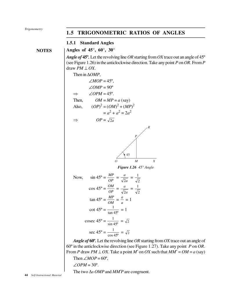
Angles of 45°, 60°, 30°
Angle of 45º. Let the revolving line OR starting from OX trace out an angle of 45º
(see Figure 1.26) in the anticlockwise direction. Take any point P on OR. From P
draw PM ⊥ OX.
Then in ∆OMP,
∠MOP = 45º,
∠OMP = 90º
⇒ ∠OPM = 45º.
Then, OM = MP = a (say)
Also, (OP)2 = (OM)2 + (MP)2
= a2 + a2 = 2a2
⇒ OP = 2a
45
O M X
P
R
Figure 1.26 45° Angle
Now, sin 45º =MP
OP =
a
a2 =
1
2
cos 45º =OM
OP =
a
a2 =
1
2
tan 45º =MP
OM =
a
a = 1
cot 45º =1
45tan º = 1
cosec 45º =1
45sin º = 2
sec 45º =1
45cos º = 2
Angle of 60º. Let the revolving line OR starting from OX trace out an angle of
60º in the anticlockwise direction (see Figure 1.27). Take any point P on OR.
From P draw PM ⊥ OX. Take a point M′ on OX such that MM′ = OM = a (say)
Then ∠MOP = 60º,
∠OPM = 30º.
The two ∆s OMP and MM′P are congruent.
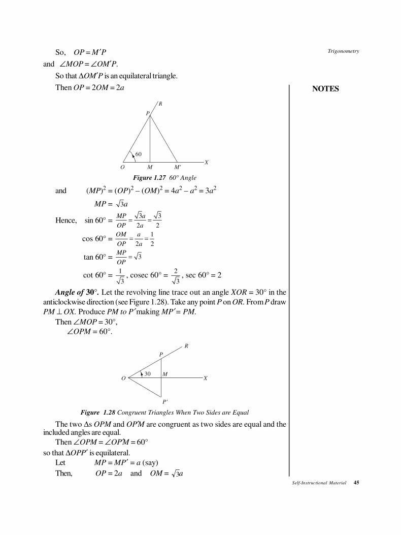
Trigonometry
NOTES
Self-Instructional Material 45
So, OP = M ′P
and ∠MOP = ∠OM′P.
So that ∆OM′P is an equilateral triangle.
Then OP = 2OM = 2a
60
O MX
P
R
M'
Figure 1.27 60° Angle
and (MP)2 = (OP)2 – (OM)2 = 4a2 – a2 = 3a
2
MP = 3a
Hence, sin 60° = 3 3
2 2
MP a
OP a= =
cos 60° =1
.2 2
OM a
OP a= =
tan 60° = 3MP
OP=
cot 60° = 1
3, cosec 60° =
2
3, sec 60° = 2
Angle of 30°. Let the revolving line trace out an angle XOR = 30° in the
anticlockwise direction (see Figure 1.28). Take any point P on OR. From P draw
PM ⊥ OX. Produce PM to P′ making MP′ = PM.
Then ∠MOP = 30°,
∠OPM = 60°.
30O X
P
M
R
P'
Figure 1.28 Congruent Triangles When Two Sides are Equal
The two ∆s OPM and OP′M are congruent as two sides are equal and theincluded angles are equal.
Then ∠OPM = ∠OP′M = 60°
so that ∆OPP′ is equilateral.
Let MP = MP′ = a (say)
Then, OP = 2a and OM = 3a
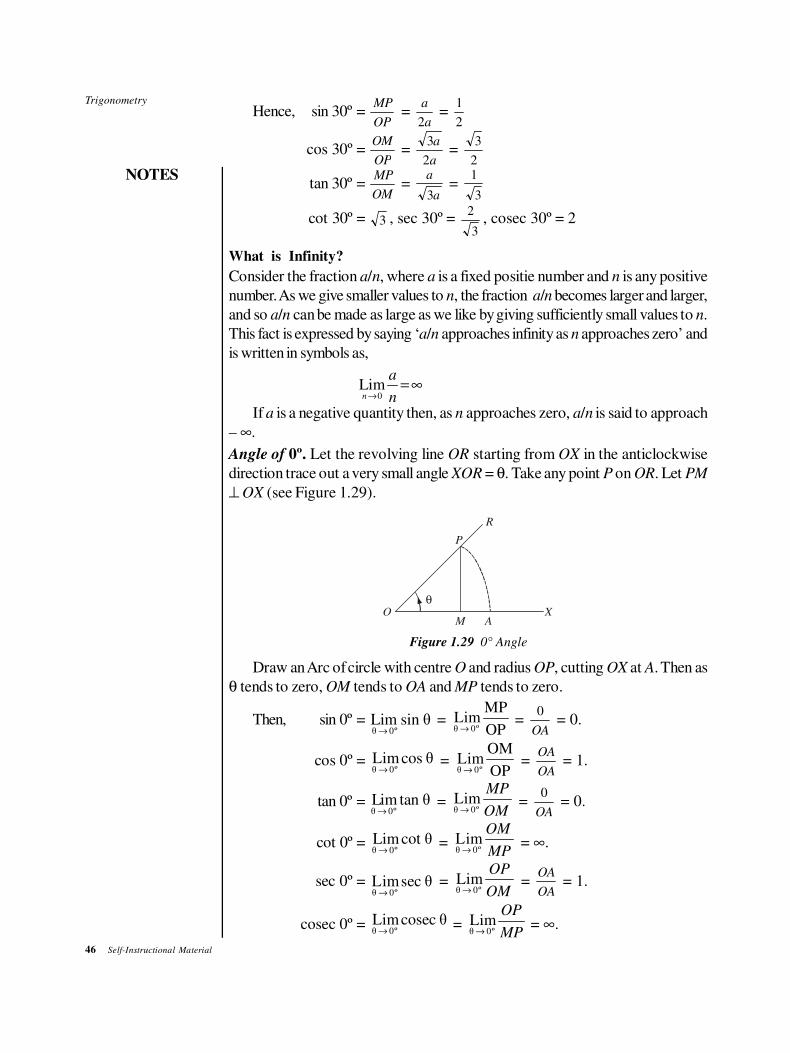
46 Self-Instructional Material
Trigonometry
NOTES
Hence, sin 30º =MP
OP =
a
a2 =
1
2
cos 30º =OM
OP =
3
2
a
a =
3
2
tan 30º =MP
OM =
a
a3 =
1
3
cot 30º = 3 , sec 30º = 2
3, cosec 30º = 2
What is Infinity?
Consider the fraction a/n, where a is a fixed positie number and n is any positive
number. As we give smaller values to n, the fraction a/n becomes larger and larger,
and so a/n can be made as large as we like by giving sufficiently small values to n.
This fact is expressed by saying ‘a/n approaches infinity as n approaches zero’ and
is written in symbols as,
0Limn
a
n→= ∞
If a is a negative quantity then, as n approaches zero, a/n is said to approach
– ∞.
Angle of 0º. Let the revolving line OR starting from OX in the anticlockwise
direction trace out a very small angle XOR = θ. Take any point P on OR. Let PM
⊥ OX (see Figure 1.29).
q
O X
P
M
R
A
Figure 1.29 0° Angle
Draw an Arc of circle with centre O and radius OP, cutting OX at A. Then as
θ tends to zero, OM tends to OA and MP tends to zero.
Then, sin 0º =θ 0ºLim sin θ
→ =
θ 0º
MPLim
OP→ =
0
OA = 0.
cos 0º =θ 0ºLimcos θ
→ =
θ 0º
OMLim
OP→ =
OA
OA = 1.
tan 0º =θ 0ºLim tan θ
→ =
θ 0ºLim
MP
OM→ =
0
OA = 0.
cot 0º =θ 0ºLim cot θ
→ =
θ 0ºLim
OM
MP→ = ∞.
sec 0º =θ 0ºLimsec θ
→ =
θ 0ºLim
OP
OM→ =
OA
OA = 1.
cosec 0º =θ 0ºLimcosec θ
→ =
θ 0ºLim
OP
MP→ = ∞.
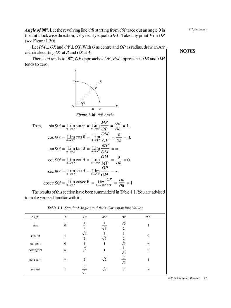
Trigonometry
NOTES
Self-Instructional Material 47
Angle of 90º. Let the revolving line OR starting from OX trace out an angle θ in
the anticlockwise direction, very nearly equal to 90º. Take any point P on OR
(see Figure 1.30).
Let PM ⊥ OX and OY ⊥ OX. With O as centre and OP as radius, draw an Arc
of a circle cutting OY at B and OX at A.
Then as θ tends to 90º, OP approaches OB, PM approaches OB and OM
tends to zero.
qO X
M
R
A
P
B
Y
Figure 1.30 90° Angle
Then, sin 90º =θ 90ºLim sin θ→
= θ 90ºLim
MP
OP→ =
OB
OB = 1.
cos 90º =θ 90ºLim cos θ→
= θ 90ºLim
OM
OP→ =
0
OB = 0.
tan 90º =θ 90ºLim tan θ→
= θ 90ºLim
MP
OM→ = ∞.
cot 90º =θ 90ºLim cot θ→
= θ 90ºLim
OM
MP→ =
0
OB = 0.
sec 90º =θ 90ºLim sec θ→
= θ 90ºLim
OP
OM→ = ∞.
cosec 90º =θ 90ºLim cosec θ→
= 90º
LimOP
MPθ → =
OB
OB = 1.
The results of this section have been summarized in Table 1.1. You are advised
to make yourself familiar with it.
Table 1.1 Standard Angles and their Corresponding Values
Angle 0º 30º 45º 60º 90º
sine 01
2
1
2
3
21
cosine 13
2
1
2
1
20
tangent 0 1 1 3 ∞
cotangent ∞ 3 11
30
cosecant ∞ 2 22
31
secant 12
32 2 ∞
48 Self-Instructional Material
Trigonometry
NOTES
Example 1.46: Find the value of cot 60º tan 30º + sec2 45º.
Solution: cot 60º tan 30º + sec2 45º = 1
3
1
32+ =
1
32+ =
7
3
Example 1.47: Find x, if tan2 45º – cos2 60º = x sin 45º cos 45º tan 60º.
Solution: LHS = 11
4− =
3
4
RHS = x1
2
1
23 =
3
2
x
Then3
4=
3
2
x⇒ x =
3
2
Example 1.48: If θ = 30º, verify that:
(i) sin 3θ = 3 sin θ – 4 sin3 θ
(ii) cos 3θ = 4 cos3 θ – 3 cos θ.
Solution: (i) sin 3θ = sin 90º = 1
and 3 sin θ – 4 sin3 θ = 3 sin 30º – 4 sin3 30º
=3
2
4
8− =
3
2
1
2− = 1.
This proves that sin 3θ = 3 sin θ – 4 sin3 θ
(ii) when θ = 30°, cos 3θ = cos 90º = 0
and 4 cos3 θ – 3 cos θ = 4 cos3 30° – 3 cos 30º
= 43 3
83
3
2− = 0.
Example 1.49: Find a solution of the following equation:
cot θ + tan θ = 2 cosec θ.
Solution: cot θ + tan θ = 1
tantan
θθ+ =
12+ tan
tan
θ
θ =
sec
tan
2 θ
θ.
Then,sec
tan
2 θ
θ= 2 cosec θ
⇒ sec2 θ = 2 cosec θ tan θ = 2 sec θ
⇒ sec θ (sec θ – 2) = 0
⇒ sec θ = 0 or 2.
As sec θ = 0 is impossible.
we get sec θ = 2 ⇒ one value of θ = π/3.
Thus, a solution of given equation is θ = π/3.
Example 1.50: Prove that cot 30º, cot 45º, and cot 60º are in G.P.
Solution: Now, cot 30º = 3 = a (say)
cot 45º = 1 = b (say)
cot 60º =1
3 = c (say)
Then, b2 = 1 = ac.
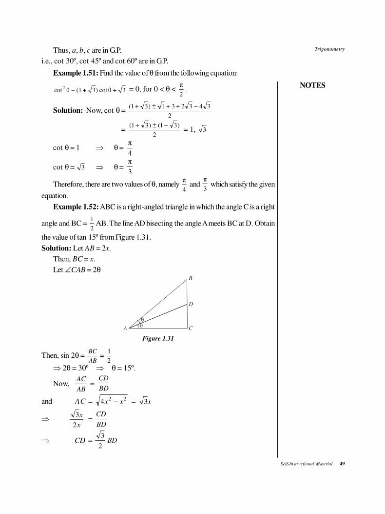
Trigonometry
NOTES
Self-Instructional Material 49
Thus, a, b, c are in G.P.
i.e., cot 30º, cot 45º and cot 60º are in G.P.
Example 1.51: Find the value of θ from the following equation:
2cot θ – (1 + 3) cotθ + 3 = 0, for 0 < θ <
π
2.
Solution: Now, cot θ = ( )1 3 1 3 2 3 4 3
2
+ ± + + −
= ( ) ( )1 3 1 3
2
+ ± − = 1, 3
cot θ = 1 ⇒ θ = π
4
cot θ = 3 ⇒ θ = π
3
Therefore, there are two values of θ, namely π
4 and
π
3 which satisfy the given
equation.
Example 1.52: ABC is a right-angled triangle in which the angle C is a right
angle and BC = 1
2 AB. The line AD bisecting the angle A meets BC at D. Obtain
the value of tan 15º from Figure 1.31.
Solution: Let AB = 2x.
Then, BC = x.
Let ∠CAB = 2θ
A C
D
B
Figure 1.31
Then, sin 2θ = BC
AB =
1
2
⇒ 2θ = 30º ⇒ θ = 15º.
Now, AC
AB =
CD
BD
and AC = 4 2 2x x− = 3x
⇒3
2
x
x=
CD
BD
⇒ CD =3
2BD
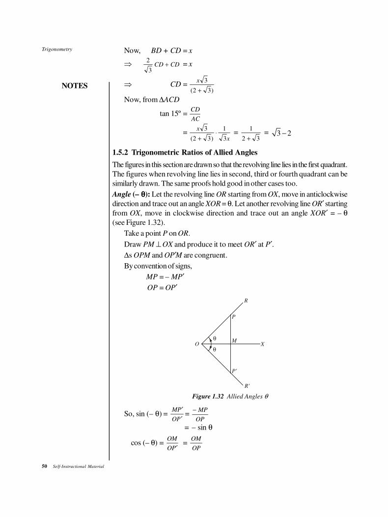
50 Self-Instructional Material
Trigonometry
NOTES
Now, BD + CD = x
⇒2
3CD CD+ = x
⇒ CD =x 3
2 3( )+
Now, from ∆ACD
tan 15º =CD
AC
=x
x
3
2 3
1
3( )+⋅ =
1
2 3+ = 3 2−
1.5.2 Trigonometric Ratios of Allied Angles
The figures in this section are drawn so that the revolving line lies in the first quadrant.
The figures when revolving line lies in second, third or fourth quadrant can be
similarly drawn. The same proofs hold good in other cases too.
Angle (– θθθθ): Let the revolving line OR starting from OX, move in anticlockwise
direction and trace out an angle XOR = θ. Let another revolving line OR′ starting
from OX, move in clockwise direction and trace out an angle XOR′ = – θ(see Figure 1.32).
Take a point P on OR.
Draw PM ⊥ OX and produce it to meet OR′ at P′.
∆s OPM and OP′M are congruent.
By convention of signs,
MP = – MP′
OP = OP′
OM
X
P
P'
R
R'
q
q
Figure 1.32 Allied Angles θ
So, sin (– θ) = MP
OP
′
′=
− MP
OP
= – sin θ
cos (– θ) =OM
OP′=
OM
OP
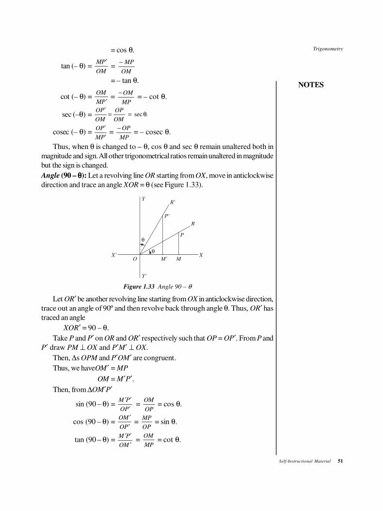
Trigonometry
NOTES
Self-Instructional Material 51
= cos θ.
tan (– θ) =MP
OM
′=
− MP
OM
= – tan θ.
cot (– θ) =OM
MP′ =
− OM
MP = – cot θ.
sec (–θ) = sec .OP OP
OM OM
′= = θ
cosec (– θ) =OP
MP
′
′ =
− OP
MP = – cosec θ.
Thus, when θ is changed to – θ, cos θ and sec θ remain unaltered both in
magnitude and sign. All other trigonometrical ratios remain unaltered in magnitude
but the sign is changed.
Angle (90 – θθθθ): Let a revolving line OR starting from OX, move in anticlockwise
direction and trace an angle XOR = θ (see Figure 1.33).
q
q
P'
R'
P
R
XM' M
X'
Y'
Y
O
Figure 1.33 Angle 90 – θ
Let OR′ be another revolving line starting from OX in anticlockwise direction,
trace out an angle of 90º and then revolve back through angle θ. Thus, OR′ has
traced an angle
XOR′ = 90 – θ.
Take P and P′ on OR and OR′ respectively such that OP = OP′. From P and
P′ draw PM ⊥ OX and P′M′ ⊥ OX.
Then, ∆s OPM and P′OM′ are congruent.
Thus, we haveOM′ = MP
OM = M′P′.
Then, from ∆OM′P′
sin (90 – θ) =M P
OP
′ ′
′ =
OM
OP = cos θ.
cos (90 – θ) =OM
OP
′
′ =
MP
OP = sin θ.
tan (90 – θ) =M P
OM
′ ′
′ =
OM
MP = cot θ.
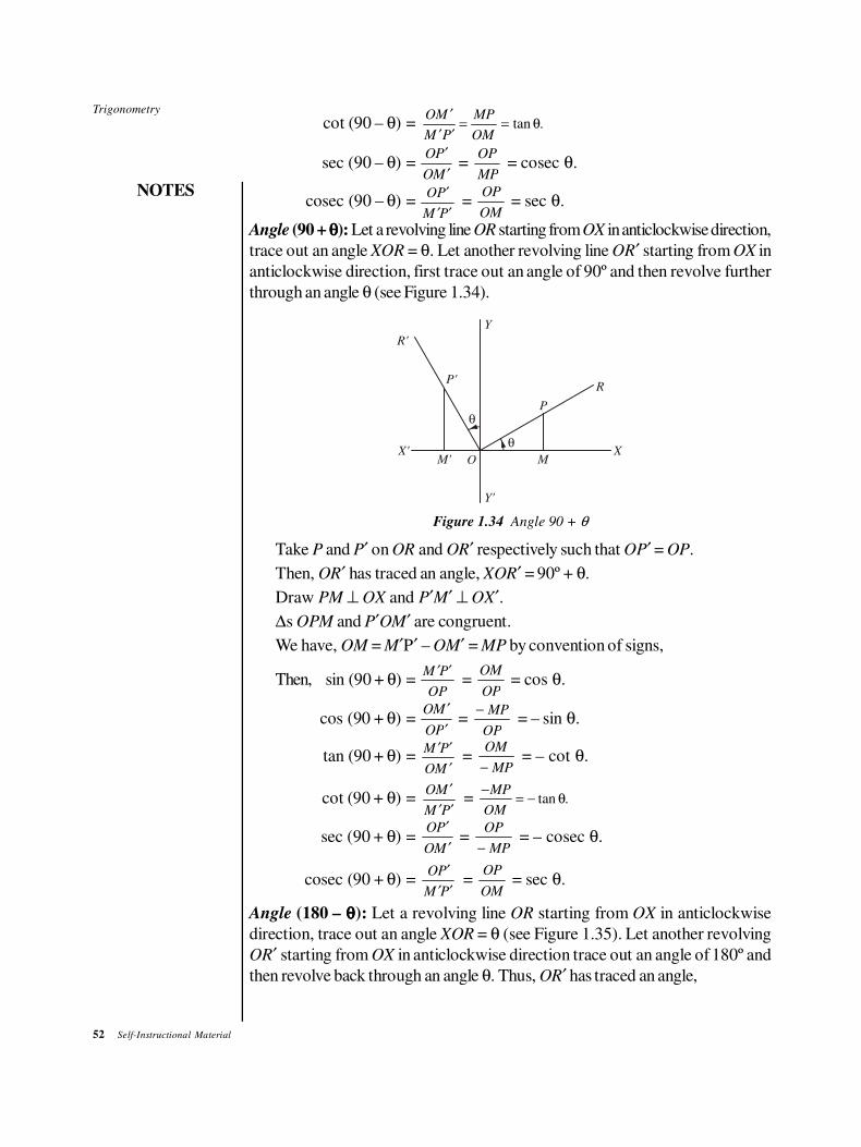
52 Self-Instructional Material
Trigonometry
NOTES
cot (90 – θ) = tan .OM MP
M P OM
′= = θ
′ ′
sec (90 – θ) =OP
OM
′
′ =
OP
MP = cosec θ.
cosec (90 – θ) =OP
M P
′
′ ′ =
OP
OM = sec θ.
Angle (90 + θθθθ): Let a revolving line OR starting from OX in anticlockwise direction,
trace out an angle XOR = θ. Let another revolving line OR′ starting from OX in
anticlockwise direction, first trace out an angle of 90º and then revolve further
through an angle θ (see Figure 1.34).
q
q
P'
R'
P
R
XM' M
X'
Y'
Y
O
Figure 1.34 Angle 90 + θ
Take P and P′ on OR and OR′ respectively such that OP′ = OP.
Then, OR′ has traced an angle, XOR′ = 90º + θ.
Draw PM ⊥ OX and P′M′ ⊥ OX′.
∆s OPM and P′OM′ are congruent.
We have, OM = M′P′ – OM′ = MP by convention of signs,
Then, sin (90 + θ) =M P
OP
′ ′ =
OM
OP = cos θ.
cos (90 + θ) =OM
OP
′
′ =
− MP
OP = – sin θ.
tan (90 + θ) = M P
OM
′ ′
′ =
OM
MP− = – cot θ.
cot (90 + θ) = OM
M P
′
′ ′ = tan .
MP
OM
−= − θ
sec (90 + θ) = OP
OM
′
′ =
OP
MP− = – cosec θ.
cosec (90 + θ) = OP
M P
′
′ ′ =
OP
OM = sec θ.
Angle (180 – θθθθ): Let a revolving line OR starting from OX in anticlockwise
direction, trace out an angle XOR = θ (see Figure 1.35). Let another revolving
OR′ starting from OX in anticlockwise direction trace out an angle of 180º and
then revolve back through an angle θ. Thus, OR′ has traced an angle,
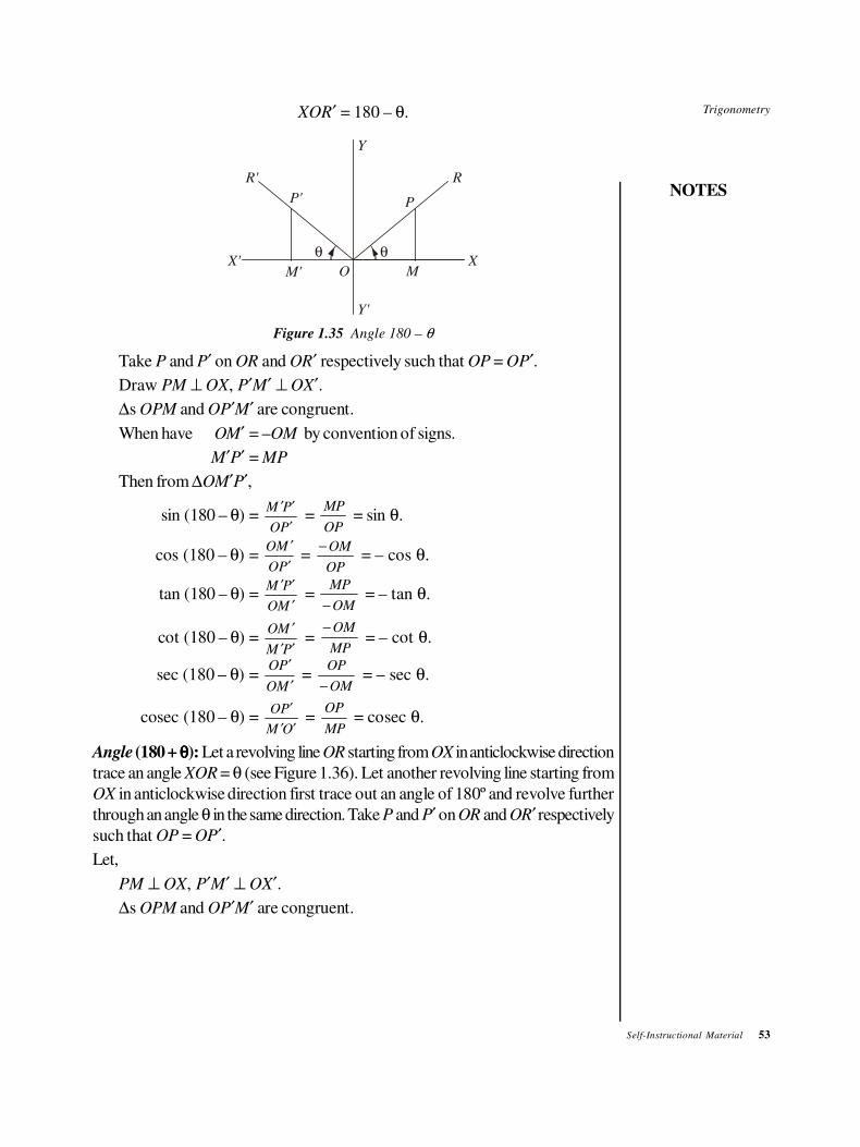
Trigonometry
NOTES
Self-Instructional Material 53
XOR′ = 180 – θ.
q q
O MXX'
Y'
Y
R' R
P
M'
P'
Figure 1.35 Angle 180 – θ
Take P and P′ on OR and OR′ respectively such that OP = OP′.
Draw PM ⊥ OX, P′M′ ⊥ OX′.
∆s OPM and OP′M′ are congruent.
When have OM′ = –OM by convention of signs.
M′P′ = MP
Then from ∆OM′P′,
sin (180 – θ) =M P
OP
′ ′
′ =
MP
OP = sin θ.
cos (180 – θ) =OM
OP
′
′ =
− OM
OP = – cos θ.
tan (180 – θ) =M P
OM
′ ′
′ =
MP
OM− = – tan θ.
cot (180 – θ) =OM
M P
′
′ ′ =
− OM
MP = – cot θ.
sec (180 – θ) =OP
OM
′
′ =
OP
OM− = – sec θ.
cosec (180 – θ) =OP
M O
′
′ ′ =
OP
MP = cosec θ.
Angle (180 + θθθθ): Let a revolving line OR starting from OX in anticlockwise direction
trace an angle XOR = θ (see Figure 1.36). Let another revolving line starting from
OX in anticlockwise direction first trace out an angle of 180º and revolve further
through an angle θ in the same direction. Take P and P′ on OR and OR′ respectively
such that OP = OP′.
Let,
PM ⊥ OX, P′M′ ⊥ OX′.
∆s OPM and OP′M′ are congruent.
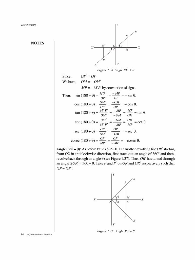
54 Self-Instructional Material
Trigonometry
NOTES
q
qOM'
MXX'
Y'
Y
R'
R
P
P'
Figure 1.36 Angle 180 + θ
Since, OP′ = OP
We have, OM = – OM′
MP = – M′P′ by convention of signs.
Then, sin (180 + θ) =M P
OP
′ ′
′ =
− MP
OP = – sin θ.
cos (180 + θ) =OM
OP
′
′ =
− OM
OP = – cos θ.
tan (180 + θ) =M P
OM
′ ′
′ =
−
−
MP
OM =
MP
OM = tan θ.
cot (180 + θ) =OM
M P
′
′ ′ =
−
−
OM
MP =
OM
MP = cot θ.
sec (180 + θ) =OP
OM
′
′ =
OP
OM− = – sec θ.
cosec (180 + θ) =OP
MP
′
′ =
OP
MP− = – cosec θ.
Angle (360 – θθθθ): As before let ∠XOR = θ. Let another revolving line OR′ starting
from OX in anticlockwise direction, first trace out an angle of 360º and then,
revolve back through an angle θ (see Figure 1.37). Thus, OR′ has turned through
an angle XOR′ = 360 – θ. Take P and P′ on OR and OR′ respectively such that
OP = OP′.
X'M
X
P
P'
R
R'
q
q M'
Y'
Y
O
Figure 1.37 Angle 360 – θ
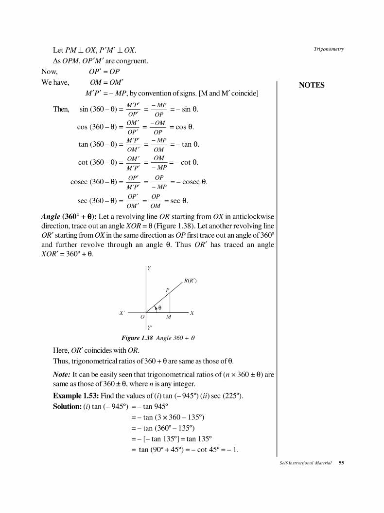
Trigonometry
NOTES
Self-Instructional Material 55
Let PM ⊥ OX, P′M′ ⊥ OX.
∆s OPM, OP′M ′ are congruent.
Now, OP′ = OP
We have, OM = OM′
M′P′ = – MP, by convention of signs. [M and M′ coincide]
Then, sin (360 – θ) =M P
OP
′ ′
′ =
− MP
OP = – sin θ.
cos (360 – θ) =OM
OP
′
′ =
− OM
OP = cos θ.
tan (360 – θ) =M P
OM
′ ′
′ =
− MP
OM = – tan θ.
cot (360 – θ) =OM
M P
′
′ ′ =
OM
MP−= – cot θ.
cosec (360 – θ) =OP
M P
′
′ ′ =
OP
MP− = – cosec θ.
sec (360 – θ) =OP
OM
′
′ =
OP
OM = sec θ.
Angle (360° + θθθθ): Let a revolving line OR starting from OX in anticlockwise
direction, trace out an angle XOR = θ (Figure 1.38). Let another revolving line
OR′ starting from OX in the same direction as OP first trace out an angle of 360º
and further revolve through an angle θ. Thus OR′ has traced an angle
XOR′ = 360º + θ.
q
O MXX'
Y'
Y
R R( )′
P
Figure 1.38 Angle 360 + θ
Here, OR′ coincides with OR.
Thus, trigonometrical ratios of 360 + θ are same as those of θ.
Note: It can be easily seen that trigonometrical ratios of (n × 360 ± θ) are
same as those of 360 ± θ, where n is any integer.
Example 1.53: Find the values of (i) tan (– 945º) (ii) sec (225º).
Solution: (i) tan (– 945º) = – tan 945º
= – tan (3 × 360 – 135º)
= – tan (360º – 135º)
= – [– tan 135º] = tan 135º
= tan (90º + 45º) = – cot 45º = – 1.
56 Self-Instructional Material
Trigonometry
NOTES
(ii) sec 225º = sec (180º + 45º) = – sec 45º = − 2 .
Example 1.54: If cos θ = a, find the values of cosec2
π + θ
and
3sin
2
π − θ
.
Solution: Now, cosec π
θ2
+FHGIKJ = sec θ =
1
cos θ =
1
a
and sin3
2
πθ−
FHG
IKJ = sin π
πθ+ −
FHG
IKJ2
= − −FHGIKJsin
πθ
2 = – cos θ = – a.
Example 1.55: Find the trigonometrical ratios of 270º – θ in terms of those of
θ for all vlaues of θ.
Solution: sin (270º – θ) = sin sin º º180 90+ − θe j= – sin (90° – θ) = – cos θ.
cos (270º – θ) = cos º º180 90+ − θe j= – cos (90º – θ) = – sin θ.
tan (270º – θ) = tan º º180 90+ − θe j= tan (90º – θ) = cot θ.
cot (270º – θ) = cot º º180 90+ − θe j= cot (90º – θ) = tan θ.
sec (270º – θ) = sec º º180 90+ − θe j= – sec (90º – θ) = – cosec θ.
cosec (270º – θ) = cosec 180 90º º+ − θe j= – cosec (90º – θ) = – sec θ.
Example 1.56: What value of x between 0º and 90º will satisfy the equation
tan 2x tan 4x = 1?
Solution: tan 2x tan 4x = 1
⇒ tan 2x =1
4tan x = cot 4x
⇒ tan 2x = tanπ
24−
FHG
IKJx
⇒ 2x =π
24− x , or 2x = π
π+ −FHG
IKJ2
4x ,
or 2x = 22
4ππ
+ −FHG
IKJx
⇒ x =15º, 45º, 75º.
Trigonometry
NOTES
Self-Instructional Material 57
Example 1.57: Find the value of tan 5º tan 25º tan 45º tan 65º tan 85º.
Solution: Now, tan 85º = tan (90º – 5º) = cot 5º
and tan 65º = tan (90º – 25º) = cot 25º
So, tan 5º tan 25º tan 45º tan 65º tan 85º
= (tan 5º cot 5º)(tan 25º cot 25º) tan 45º
= tan 45º = 1.
Example 1.58: Show that:
3 3
2
sin (270º + θ) cos (720º – θ) – sin (270º – θ) sin (540º + θ)
sin (90º + θ) sin (– θ)– cos (280º – θ) 2
cot (270º – θ)+
cosec (450º + θ) = 1.
where θ is taken such as the denominator appearing in any fraction in the
expression does not vanish.
Solution: Now, cos3 (720º – θ) = cos3 θ
sin3 (540º + θ) = – sin3 θ
cosec2 (450º + θ) = sec2 θ
sin (270º + θ) = – cos θ
sin (270º – θ) = – cos θ
cot (270º – θ) = tan θ
So, the given expression is equal to,
=
3 3
2 2
cos cos sin cos tan
cos sin cos sec
− θ θ − θ θ θ+
− θ θ − θ θ
= − +
− ++
cos (sin cos )
cos (sin cos )
sin cosθ θ θ
θ θ θ
θ θ3 3
1
= − + + −
− ++
(sin cos )(sin cos sin cos )
(sin cos )
sin cosθ θ θ θ θ θ
θ θ
θ θ2 2
1
= 1 – sin θ cos θ + sin θ cos θ = 1.
Example 1.59: If θ is the angle in the fourth quadrant satisfying the equation
cot2 θ = 4, find the vlaue of 1
5 (sec θ – cosec θ).
Solution: cot2 θ = cosec2 θ – 1
⇒ 4 = cosec2 θ – 1
⇒ cosec2 θ = 5
⇒ cosec θ = − 5 (as θ lies in fourth quadrant)
Also cot2 θ = 4 ⇒ tan2 θ = 1
4
So, tan2 θ = sec2 θ – 1
⇒1
4= sec2 θ – 1 ⇒ sec2 θ =
5
4
⇒ sec θ = 5
2
58 Self-Instructional Material
Trigonometry
NOTES
Therefore, 1
5(sec )θ θ− cosec =
1
5
5
25+
FHG
IKJ =
3
2.
CHECK YOUR PROGRESS
10. If θ is an acute angle, find its value from tan θ = 2 sin θ.
11. If A, B, C are angles of a triangle, prove that:
cot (A + B) + cot C = 0.
12. In any triangle ABC, 2 sin A + 3 sin B = 5
2 and 3 sin A + 2 sin B
= 3 3
2. Find the angle C.
13. Given that θ is an angle between 180º and 270º. Find the value of θ if it
satisfies the equation 3 cos2 θ – sin2 θ = 1.
1.6 INVERSE TRIGONOMETRIC FUNCTIONS
The inverse sine function is written as:
y = sin– 1x, which implies that x = sin y, − ≤ ≤
1
2
1
2π πy
Note: sin– 1x ≠ (sin x)– 1
(sin x)– 1 =1
sin x and sin (sin– 1
x) = x
cos (cos– 1x) = x, cos– 1(cos x) = x
sin− FHGIKJ
1 1
2 =
π
4 since sin
π
4 =
1
2
sin− −FHGIKJ
1 1
2= −
π
4 since sin −
FHGIKJ
π
4 = − sin
π
4 = −
1
2
Other trigonometric inverse functions are cos– 1x, tan– 1
x, sec– 1x, cosec– 1
x,
cot– 1x.
cos− FHGIKJ
1 1
2 =
π
4, since cos
π
4 =
1
2.
Example 1.60: Prove cos– 1x =
1
2
1π − −sin x for |x| ≤ 1.
Solution: Let cos– 1x = y ∴ cos y = x or sin
π
2−FHGIKJy = x
∴ sin– 1x =
π
2− y =
π
2
1− −cos x . ⇒ cos–1 x = 2
π – sin–1
x Hence proved.
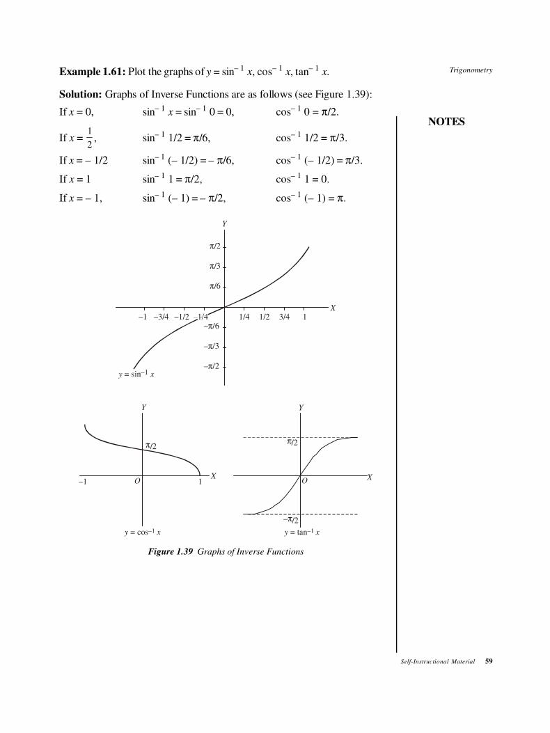
Trigonometry
NOTES
Self-Instructional Material 59
Example 1.61: Plot the graphs of y = sin– 1x, cos– 1
x, tan– 1x.
Solution: Graphs of Inverse Functions are as follows (see Figure 1.39):
If x = 0, sin– 1x = sin– 1 0 = 0, cos– 1 0 = π/2.
If x = 1
2, sin– 1 1/2 = π/6, cos– 1 1/2 = π/3.
If x = – 1/2 sin– 1 (– 1/2) = – π/6, cos– 1 (– 1/2) = π/3.
If x = 1 sin– 1 1 = π/2, cos– 1 1 = 0.
If x = – 1, sin– 1 (– 1) = – π/2, cos– 1 (– 1) = π.
1/4 1/2 3/4 1–1/2–3/4–1– /6π
– /3π
– /2π
π/6
π/3
π/2
X
y x = sin –1
Y
Y
–1 O 1X
π/2
y x = cos –1
Y
π/2
OX
– /2π
y x = tan –1
Figure 1.39 Graphs of Inverse Functions
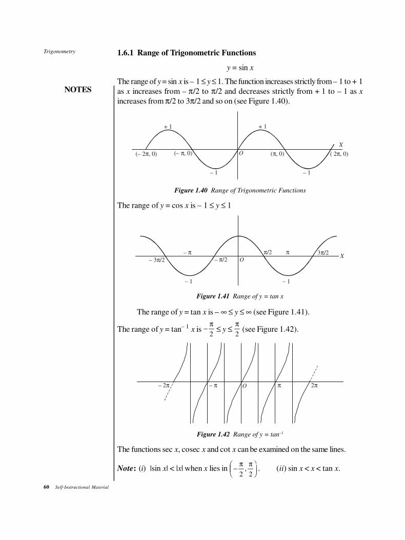
60 Self-Instructional Material
Trigonometry
NOTES
1.6.1 Range of Trigonometric Functions
y = sin x
The range of y = sin x is – 1 ≤ y ≤ 1. The function increases strictly from – 1 to + 1
as x increases from – π/2 to π/2 and decreases strictly from + 1 to – 1 as x
increases from π/2 to 3π/2 and so on (see Figure 1.40).
+ 1 + 1
– 1– 1
(– 2 , 0)π (– , 0)π O ( , 0)π ( 2 , 0)π
X
Figure 1.40 Range of Trigonometric Functions
The range of y = cos x is – 1 ≤ y ≤ 1
– 3 /2π
– π – /2π O
π/2 π 3 /2πX
– 1 – 1
Figure 1.41 Range of y = tan x
The range of y = tan x is – ∞ ≤ y ≤ ∞ (see Figure 1.41).
The range of y = tan– 1x is −
π
2 ≤ y ≤
π
2 (see Figure 1.42).
– 2π – π 2πO π
Figure 1.42 Range of y = tan–1
The functions sec x, cosec x and cot x can be examined on the same lines.
Note: (i) |sin x| < |x| when x lies in −FHG
IKJ
π π
2 2, . (ii) sin x < x < tan x.
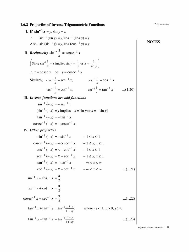
Trigonometry
NOTES
Self-Instructional Material 61
1.6.2 Properties of Inverse Trigonometric Functions
I. If sin– 1 x = y, sin y = x
∴ sin– 1 (sin y) = y, cos– 1 (cos y) = y
Also, sin (sin– 1y) = y, cos (cos– 1
y) = y
II. Reciprocity –1 1
sinx
= cosec– 1 x
-1 1 1 1Since sin = implies sin = or =
siny y x
x x y
∴ x = cosec y or y = cosec– 1x
Similarly, cos−1 1
x= sec– 1
x, sec−1 1
x = cos– 1
x
tan−1 1
x= cot– 1
x, cot−1 1
x = tan– 1
x ...(1.20)
III. Inverse functions are odd functions
sin– 1 (– x) = – sin– 1x
[sin– 1 (– x) = y implies – x = sin y or x = – sin y]
tan– 1 (– x) = – tan– 1x
cosec– 1 (– x) = – cosec– 1x
IV. Other properties
sin– 1 (– x) = – sin– 1x – 1 ≤ x ≤ 1
cosec– 1 (– x) = – cosec– 1x – 1 ≥ x, x ≥ 1
cos– 1 (– x) = π – cos– 1x – 1 ≤ x ≤ 1
sec– 1 (– x) = π – sec– 1x – 1 ≥ x, x ≥ 1
tan– 1 (– x) = – tan– 1x – ∞ < x < ∞
cot– 1 (– x) = π – cot– 1x – ∞ < x < ∞ ...(1.21)
sin– 1x + cos– 1
x =π
2
tan– 1x + cot– 1
x =π
2
cosec– 1x + sec– 1
x =π
2...(1.22)
tan– 1x + tan– 1
y = tan− +
−
1
1
x y
xy, where xy < 1, x > 0, y > 0
tan– 1x – tan– 1
y = tan− −
+
1
1
x y
xy...(1.23)
62 Self-Instructional Material
Trigonometry
NOTES
x, y > 0
For example, if sin– 1x = θ
x = sin θ = cosπ
θ2
−FHGIKJ
∴ cos– 1x =
πθ
2−
∴ sin– 1x + cos– 1
x = π
2.
1.7 TRIGONOMETRIC EQUATIONS
A trigonometric equation involves trigonometric expressions like sin θ, cos θ, etc.,
where θ is an unknown. The solution of the equation is the value or sometimes
values of θ that satisfies the equation.
Since the number of solutions of a trigonometric equation is infinite, the numeri-
cally smallest angle α is of importance, i.e., the equation sin θ = k has solutions,
θ = ( 1) ... 2, 1, 0,1, 2, 3, ...
(All integers ve or ve)
n
n I
n nπ α
∈
+ − = − − − +
Where α is numerically the smallest angle for which sin α = k
cos θ = k has solutions θ = 2nπ ± α (n ∈ I)
Where α is numercially the smallest angle for which cos α = k.
Similarly, for tan θ = k, the solutions are θ = nπ + α (n ∈ I)
Where α is numerically the smallest angle for which tan α = k.
Example 1.62: 2 3 12sin cosθ θ+ + = 0, 0 ≤ θ ≤ π
Solution:
2 1 3 12( cos ) cos− + +θ θ = 0 i.e., 2 32cos cosθ θ− – 3 = 0
∴ (cos )( cos )θ θ− +3 2 3 = 0
cos θ = 3 not possible; cos θ = −3
2or θ = α =
5
6
πor
7
6
π.
Since θ has between 0 and π, 6
π is discarded. Hence, θ =
5
6
π
Example 1.63: Given the usual trigonometric ratios, find the trigonometric ratios
of 18º, 36º, 54º, 72º.
Solution: Let A = 18º then, 2A = 36º = 90º – 3A
Trigonometry
NOTES
Self-Instructional Material 63
sin 2A = sin (90 – 3A) = cos 3A
i.e., 2 sin A cos A = 4 cos3A – 3 cos A
∴ cos A(2 sin A – 4 cos2A + 3) = 0
Since, cos A ≠ 0, 2 sin A – 4 cos2A + 3 = 0
∴ 2 sin A – 4(1 – sin2A) + 3 = 0
∴ 4 sin2A + 2 sin A – 1 = 0 (compare with ax
2 + bx + c = 0)
∴ sin A = sin 18º = 2 2 5
8
− ± =
1 5
4
− ±
∴ sin 18º =1 5
4
− +, a positive value
or =− −1 5
4, a negative value is not possible in the first quadrant.
Hence, sin 18° = 5 1
4
−
∴ cos 18º = 1 182− sin º = 10 2 5
4
+
tan 18º =5 1
10 2 5
−
+
sin 36º = 2 sin 18º cos 18º = 2
165 1 10 2 5( )( )− +
= 10 2 5
4
−
cos 36º =5 1
4
+
tan 36º =5 1
10 2 5
+
−
Since, cos (90 – 2A) = sin 2A
i.e., cos 54º = sin 36º = 10 2 5
4
−
sin 54º = cos 36º = 5 1
4
+
sin 72º = cos 18º = 10 2 5
4
+
cos 72º = sin 18º = 5 1
4
−.
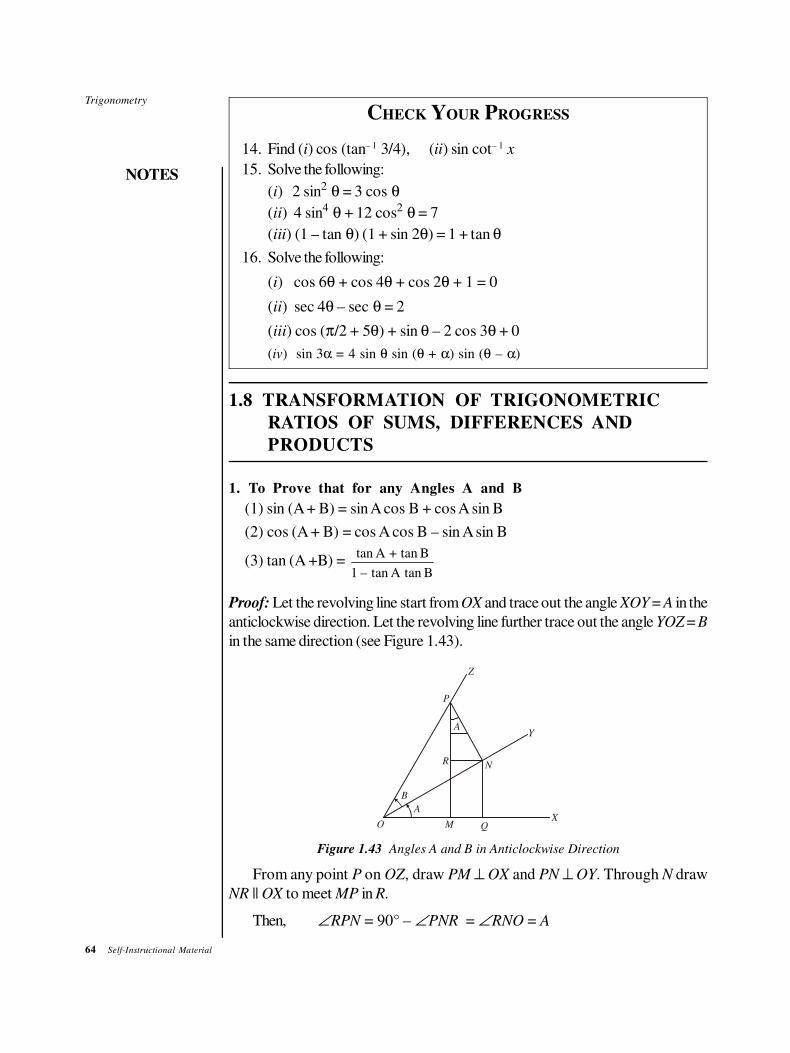
64 Self-Instructional Material
Trigonometry
NOTES
CHECK YOUR PROGRESS
14. Find (i) cos (tan– 1 3/4), (ii) sin cot– 1 x
15. Solve the following:
(i) 2 sin2 θ = 3 cos θ
(ii) 4 sin4 θ + 12 cos2 θ = 7
(iii) (1 – tan θ) (1 + sin 2θ) = 1 + tan θ
16. Solve the following:
(i) cos 6θ + cos 4θ + cos 2θ + 1 = 0
(ii) sec 4θ – sec θ = 2
(iii) cos (π/2 + 5θ) + sin θ – 2 cos 3θ + 0
(iv) sin 3α = 4 sin θ sin (θ + α) sin (θ – α)
1.8 TRANSFORMATION OF TRIGONOMETRIC
RATIOS OF SUMS, DIFFERENCES AND
PRODUCTS
1. To Prove that for any Angles A and B
(1) sin (A + B) = sin A cos B + cos A sin B
(2) cos (A + B) = cos A cos B – sin A sin B
(3) tan (A +B) = tan A + tan B
1 – tan A tan B
Proof: Let the revolving line start from OX and trace out the angle XOY = A in the
anticlockwise direction. Let the revolving line further trace out the angle YOZ = B
in the same direction (see Figure 1.43).
Z
Y
XO
B
A
A
P
R
M Q
N
Figure 1.43 Angles A and B in Anticlockwise Direction
From any point P on OZ, draw PM ⊥ OX and PN ⊥ OY. Through N draw
NR || OX to meet MP in R.
Then, ∠RPN = 90° – ∠PNR = ∠RNO = A
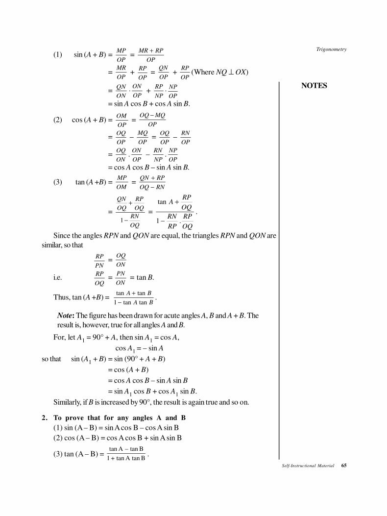
Trigonometry
NOTES
Self-Instructional Material 65
(1) sin (A + B) = OP
MP =
OP
RPMR +
= OP
MR +
OP
RP =
OP
QN +
OP
RP(Where NQ ⊥ OX)
= ON
QN⋅
OP
ON +
NP
RP⋅
OP
NP
= sin A cos B + cos A sin B.
(2) cos (A + B) = OP
OM =
OP
MQOQ −
= OP
OQ –
OP
MQ =
OP
OQ –
OP
RN
= ON
OQ.
OP
ON –
NP
RN.
OP
NP
= cos A cos B – sin A sin B.
(3) tan (A +B) = OM
MP =
RNOQ
RPQN
−
+
=
OQ
RN
OQ
RP
OQ
QN
−
+
1
=
OQ
RP
RP
RN
OQ
RPA
.1
tan
−
+
.
Since the angles RPN and QON are equal, the triangles RPN and QON are
similar, so that
PN
RP=
ON
OQ
i.e.OQ
RP=
ON
PN = tan B.
Thus, tan (A +B) = BA
BA
tantan1
tantan
−
+.
Note: The figure has been drawn for acute angles A, B and A + B. The
result is, however, true for all angles A and B.
For, let A1 = 90° + A, then sin A
1 = cos A,
cos A1
= – sin A
so that sin (A1 + B) = sin (90° + A + B)
= cos (A + B)
= cos A cos B – sin A sin B
= sin A1 cos B + cos A
1 sin B.
Similarly, if B is increased by 90°, the result is again true and so on.
2. To prove that for any angles A and B
(1) sin (A – B) = sin A cos B – cos A sin B
(2) cos (A – B) = cos A cos B + sin A sin B
(3) tan (A – B) = tan A – tan B
1 + tan A tan B.
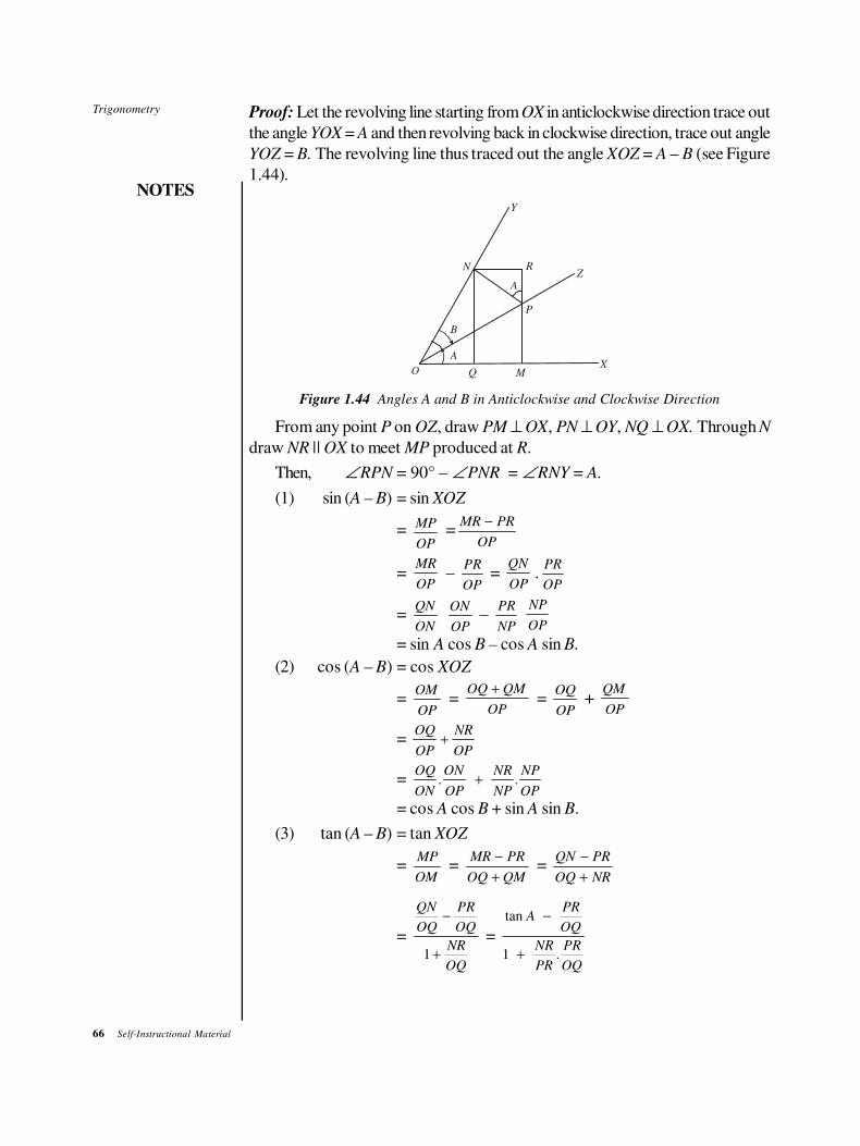
66 Self-Instructional Material
Trigonometry
NOTES
Proof: Let the revolving line starting from OX in anticlockwise direction trace out
the angle YOX = A and then revolving back in clockwise direction, trace out angle
YOZ = B. The revolving line thus traced out the angle XOZ = A – B (see Figure
1.44).
Y
Z
XO
B
A
MQ
P
A
RN
Figure 1.44 Angles A and B in Anticlockwise and Clockwise Direction
From any point P on OZ, draw PM ⊥ OX, PN ⊥ OY, NQ ⊥ OX. Through N
draw NR || OX to meet MP produced at R.
Then, ∠ RPN = 90° – ∠ PNR = ∠ RNY = A.
(1) sin (A – B) = sin XOZ
= OP
MP =
OP
PRMR −
= OP
MR –
OP
PR =
OP
QN.
OP
PR
= ON
QN
ON
OP –
NP
PR
OP
NP
= sin A cos B – cos A sin B.
(2) cos (A – B) = cos XOZ
= OP
OM =
OP
QMOQ + =
OP
OQ +
OP
QM
= OP
NR
OP
OQ+
= . .OQ ON NR NP
ON OP NP OP+
= cos A cos B + sin A sin B.
(3) tan (A – B) = tan XOZ
= OM
MP =
QMOQ
PRMR
+
− =
NROQ
PRQN
+
−
=
OQ
NR
OQ
PR
OQ
QN
+
−
1
=
tan
1 .
PRA
OQ
NR PR
PR OQ
−
+
Trigonometry
NOTES
Self-Instructional Material 67
Since the angles RPN and NOQ are equal, the triangles RPN and NOQ are
similar, so that
OQ
PR=
ON
PN = tan B
Thus tan, (A – B) = tan tan
1 tan tan
A B
A B
−
+
Note: The figure in this article is again drawn for acute angles A, B and
A +B, but the result can be proved for all angles A and B.
Trigonometrical Ratios of Multiple and Submultiple Angles to prove that:
(1) (i) sin 2A = 2 sin A cos A
(ii) cos 2A = 2 cos2 A – 1 = 1– 2 sin2 A = cos2 A – sin2 A
(iii) tan 2A = 2
2 tan A
1 – tan A
Proof: sin (A + B) = sin A cos B + cos A sin B.
Put A = B
We have, sin 2A = sin A cos A + cos A sin A
= 2 sin A cos A.
(ii) Again, cos (A + B) = cos A cos B – sin A sin B
Put A = B
We have, cos 2A = cos A cos A – sin A sin A
= cos2 A – sin2 A.
Also, cos2 A – sin2 A = (1– sin2 A) – sin2 A
= 1 – 2 sin2 A.
and cos2 A – sin2 A – cos2 A – (1 – cos2 A) = 2 cos2 A – 1.
(iii) Also, tan (A + B) = BA
BA
tantan1
tantan
−
+.
Put A = B
We have, tan 2A = AA
AA
tantan1
tantan
−
+ =
A
A
2tan1
tan2
−.
(2)(i) sin 3A = 3 sin A – 4 sin3 A
(ii) cos 3A = 4 cos3 A – 3 cos A
(iii) tan 3A = 3
2
3 tan A – tan A
1 – 3 tan A
Proof: (i) sin 3A = sin (A +2A)
= sin A cos 2A + cos A sin 2A
= sin A (1 – 2 sin2 A) + cos A (2 sin A cos A)
= sin A – 2 sin3 A + 2 sin A (1 – sin2 A)
= 3 sin A – 4 sin3 A.
68 Self-Instructional Material
Trigonometry
NOTES
(ii) cos 3A = cos (A + 2A)
= cos A cos 2A – sin A sin 2A
= cos A (2 cos2 A – 1) – sin A (2 sin A cos A)
= 2 cos3 A – cos A –2 cos A (1– cos2 A)
= 4 cos3 A – 3 cos A.
(iii) tan 3A = tan (A + 2A)
= AA
AA
2tantan1
2tantan
−
+ =
A
AA
A
AA
2
2
tan1
tan2tan1
tan1
tan2tan
−−
−+
= 2
2 2
tan (1 tan ) 2 tan
(1 tan ) 2 tan
A A A
A A
− +
− −
= A
AA
2
3
tan31
tantan3
−
−.
(3) (i) sin A = A A
2sin cos2 2
(ii) cos A= 2 2A Acos sin
2 2−
= 2 A2cos 1
2− = 2 A
1 2sin2
−
(iii) tan A = 2
A2 tan
2A
1 tan2
−
Proof: Replace A by 2
A in (1) of this subsection. All relations in (3) will immedi-
ately follow.
(4) (i) A
sin2
= 1 cos A
±2
−
(ii) A
cos2
= 1 + cos A
±2
(iii) A
tan2
= 1 cos A
±1 + cos A
−
Proof: We have cos A = 2
sin212 A
− , form (3)
Then,2
sin2 2 A= 1 – cos A
so that2
sin 2 A=
2
cos1 A−⇒
2sin
A =
2
cos1 A−±
Trigonometry
NOTES
Self-Instructional Material 69
Similarly, cos A = 12
cos2 2 −A
⇒2
cos2 2 A= 1 + cos A
⇒2
cos2 2 A=
2
cos1 A+
⇒2
cosA
= 2
cos1 A+±
Hence,2
tanA
=
2cos
2sin
A
A
= A
A
cos1
cos1
+
−±
Example 1.64: If sin α = 3
5 and cos β =
9
41, find the value of sin (α – β),
α, β being acute angles.
Solution: cos2 α = 1– sin2 α = 1 – 9
25 =
16
25
⇒ cos2 α = 4
5±
Since α is acute angle, cos α = 4
5
Also, sin2 β = 1 – cos2 β
= 1 – 81
1681 =
1600
1681
⇒ sin β = 40
41±
β is acute angle ⇒ sin β = 4 0
4 1
Therefore, sin (α – β) = sin α cos β – sin β cos α
= 3 9 40 4 27 160 133
5 41 41 5 205 205
−× − × = =
Example 1.65: Find the value of sin 18° and cos 18°.
Solution: Put 18° = x so that 90° = 5x
Then 2x = 90° – 3x
⇒ sin 2x = sin (90° – 3x) = cos 3x
or 2 sin x cos x = 4 cos3 x – 3 cos x
or 4 cos3 x – 2 sin x cos x – 3 cos x = 0
or cos x (4 cos2x – 2 sin x – 3) = 0
or 4 cos2 x – 2 sin x – 3 = 0 since cos x ≠ 0
or 4 (1 – sin2 x) – 2 sin x – 3 = 0
70 Self-Instructional Material
Trigonometry
NOTES
or 4 sin2 x + 2 sin x – 1 = 0
⇒ sin x = 2 20
8
− ± =
4
51 +− or
4
51 −−.
Since, x = 18°. sin x is positive so that the value 4
51 −− is rejected.
Hence, sin x = 4
51 +−i.e. sin 18° =
4
51 +−
Also, cos 18° = °− 18sin1 2 =
−+−
16
52151
=16 6 2 5
116
− +− =
4
5210 +.
Example 1.66: If tan θ = 12
5 and θ is in third quadrant, find the value of
2 sin 3 cos2 2
θ θ− .
Solution: θ lies in third quadrant
⇒ θ lies between 180° and 270°
⇒2
θ lies between 90° and 135°
⇒ sin 2
θ is positive and cos
2
θ is negative.
Now, tan θ = 12
5 ⇒ sin θ =
12
13
− and cos θ =
5
13
−
(as θ lies in 3rd quadrant)
Therefore, cos 2
θ= –
1 cos
2
+ θ = –
8
26
and sin2
θ=
1 cos
2
− θ =
18
26
So 2 sin 2
θ – 3 cos
2
θ=
18 82 3
26 26+ =
9 42 3
13 13+
= 1
[6 6]13
+ = 12
13.
Example 1.67: Prove that sin 5θ = 5 sin θ – 20 sin3 θ + 16 sin5 θ.
Solution: LHS = sin 5θ
= sin (2θ + 3θ)
= sin 2θ cos 3θ + cos 2θ sin 3θ
= 2 sin θ cos θ (4 cos3 θ – 3 cos θ)
+ (3 sin θ – 4 sin3 θ) (1 – 2 sin2 θ)
= 2 sin θ cos2 θ (4 cos2 θ – 3)
+ sin θ (3 – 4 sin2 θ) (1 – 2 sin2 θ)
Trigonometry
NOTES
Self-Instructional Material 71
= sin θ [2(1 – sin2 θ) (1 – 4 sin2 θ)
+ (3 – 4 sin2 θ) (1 – 2 sin2 θ)
= sin θ [2 – 10 sin2 θ + 8 sin4 θ + 3 – 10 sin2 θ + 8 sin2 θ]
= 5 sin θ – 20 sin3 θ + 16 sin5 θ.
Example 1.68: Prove that sin A + sin 3A
cos A + cos3A = tan 2A.
Solution: LHS= sin sin 3
cos cos3
A A
A A
+
+ =
3
3
sin 3sin 4 sin
cos 4 cos 3 cos
A A A
A A A
+ −
+ −
= 2
2
4 sin (1 sin )
2 cos (2 cos 1)
A A
A A
−
−
= 2
2 sin cos
cos cos 2
A A
A A
= 2 sin cos
cos 2
A A
A
= sin 2
cos 2
A
A = tan 2 A.
Example 1.69: Prove that 1 + cos2 2θ = 2 (cos4 θ + sin4 θ).
Solution: RHS = 2 (cos4 θ + sin4 θ)
= 2 [(cos2 θ – sin2 θ)2 + 2 sin2 θ cos2 θ]
= 2 [(cos 2θ)2 + 2 sin2 θ cos2 θ]
= 2 (cos 2θ)2 + 4 sin2 θ cos2 θ
= 2 (cos 2θ)2 + (sin 2θ)2
= (cos 2θ)2 + [(cos 2θ)2 + (sin 2θ)2]
= (cos 2θ)2 + 1 = LHS.
Example 1.70: If sin θ + sin φ = a, cos θ + cos φ = b, find the value of
tan2
θ − φ.
Solution: sin θ + sin φ = a
cos θ + cos φ = b
Squaring and adding, we get
(sin2 θ + cos2 θ) + (sin2 φ + cos2 φ) + 2 (sin θ sin φ + cos θ cos φ)
= a2 + b
2
⇒2 {1 + cos (θ – φ)}= a2 + b2
⇒ 1 + cos (θ – φ) = 2 2
2
a b+
Also, 1 – cos (θ – φ) = 2 2
1 12
a b +− −
= 2 2
22
a b+− =
2 24
2
a b− −
72 Self-Instructional Material
Trigonometry
NOTES
⇒ tan2
θ − φ=
1 cos ( )
1 cos ( )
− θ − φ±
+ θ − φ =
2 2
2 2
4 a b
a b
− −±
+
Example 1.71: Find the value of sin 9° and cos 9°.
Solution: Now, cos 2θ = 1 –2 sin2 θ
Put θ = 9°, we get
cos 18° = 1 – 2 sin2 9°
cos 18° = 10 2 5
4
+
So10 2 5
4
+= 1 – 2 sin2 9°
or 2 sin2 9° = 1 – 10 2 5
4
+ =
4 10 2 5
4
− +
or sin2 9° = 4 10 2 5
8
− +
or sin 9° = 4 10 2 5
8
− +±
Sin 9° is positive, so that the negative value is rejected.
Hence, sin 9° = 4 10 2 5
8
− ++
Also, cos 9° = 21 sin 9− ° = 4 10 2 5
18
− + −
= 8 4 10 2 5
8
− + + =
4 10 2 5
8
+ +
Example 1.72: Prove that tan sec 1
tan sec 1
A A
A A
+ −
− + =
1 sin
cos
A
A
+.
Solution: LHS = tan sec 1
tan sec 1
A A
A A
+ −
− + =
sin 11
cos cos
sin 11
cos cos
A
A A
A
A A
+ −
− +
= sin 1 cos
sin 1 cos
A A
A A
+ −
− + =
2
2
sin 2 sin2
sin 2 sin2
AA
AA
+
−
=
2
2
2 sin cos 2 sin2 2 2
2 sin cos 2 sin2 2 2
A A A
A A A
+
−
Trigonometry
NOTES
Self-Instructional Material 73
=
cos sin2 2
cos sin2 2
A A
A A
+
−
=
cos sin cos sin2 2 2 2
cos sin cos sin2 2 2 2
A A A A
A A A A
+ +
− +
=
2 2
2 2
cos sin 2 sin cos2 2 2 2
cos sin2 2
A A A A
A A
+ +
−
= 1 sin
cos
A
A
+ = RHS.
Example 1.73: Prove that:
θtan 45°
2
+
=
1 sin θ
1 sin θ
+
−, where 0 < θ < 90°.
Solution: LHS = tan 452
θ ° +
= tan 45 tan
2
1 tan 45 tan2
θ° +
θ− °
= 1 tan
2
1 tan2
θ+
θ−
= cos sin
2 2
cos sin2 2
θ θ+
θ θ−
=
2
2 2
cos sin2 2
cos sin2 2
θ θ +
θ θ
−
= 1 2 sin cos
2 2
cos
θ θ+
θ =
2
1 sin
1 sin
+ θ
± − θ
= 1 sin
(1 sin ) (1 sin )
+ θ
± − θ + θ =
1 sin
1 sin
+ θ±
− θ
Since 0 < θ < 90°, we have θ
2 < 45°, so that tan 45
2
θ ° +
is positive.
Thus, tan 452
° +θ
= 1 sin
1 sin
+ θ
− θ = RHS.
Example 1.74: Prove that
cos15 sin153
cos15 sin15
°+ °=
°− °
74 Self-Instructional Material
Trigonometry
NOTES
Solution: LHS= 1 tan15
1 tan15
+ °
− ° =
tan 45 tan15
1 tan 45 tan15
+
−
= tan (45 + 15) = tan 60° = 3 = RHS.
Example. 75: Prove that:
tan 2A – tan A = 2 sin
cos + cos
A
A 3A.
Solution: LHS = sin 2 sin
cos 2 cos
A A
A A−
= sin 2 cos sin cos 2
cos 2 cos
A A A A
A A
−
= sin (2 )
cos 2 cos
A A
A A
− =
sin
cos 2 cos
A
A A
= 2sin
2cos cos 2
A
A A
= 2
2sin
2cos (2cos 1)
A
A A−
= 3
2sin
4cos 2cos
A
A A−
= 3
2sin
4cos 3cos cos
A
A A A− +
= 2sin
cos3 cos
A
A A+
= 2sin
cos cos3
A
A A+
= RHS
Hence, the result follows.
Example 1.76: Prove that:
cot α = tan α + 2 tan 2α + 4 tan 4α + 8 cot 8α.Solution: Consider cot α – tan α – 2 tan 2α – 4 tan 4α – 8 cot 8α
= cos sin
sin cos
α α−
α α – 2 tan 2α – 4 tan 4α – 8 cot 8α
=cos 2α
sin α cosα – 2 tan 2α – 4 tan 4α – 8 cot 8α
=2cos 2α sin 2α
2sin 2α cos 2α
− – 4 tan 4α – 8 cot 8α
=2 2
cos 2α sin 2α2
sin 2α cos 2α
−
– 4 tan 4α – 8 cot 8α
=cos 4 sin 4
2 2 4 8 cot 8sin 4 cos 4
α α× − − α
α α
=2 2
cos 4α sin 4α4 8 cot8α
sin 4 cos 4α
−− α
Trigonometry
NOTES
Self-Instructional Material 75
=cos8α
4 2 8 cot 8αsin 8α
× − = 8 cot 8α – 8 cot 8α = 0
This proves the result.
Example 1.77: Given that:
tan A + tan B = p and tan A tan B = q
find sin2 (A + B) and cos 2 (A + B).
Solution: sin2 (A + B) = 2
1
cos ec ( )A B+ =
2
1
1 cot ( )A B+ +
=
2
1
11
tan ( )A B
++
= 2
2
tan ( )
1 tan ( )
A B
A B
+
+ +
=
2
2
2
2
(1 )
1(1 )
p
q
p
q
−
+−
= 2
2 2(1 )
p
p q+ −
and cos 2 (A + B) = cos2 (A + B) – sin2 (A + B)
= 2 2
2 2
cos ( ) sin ( )
cos ( ) sin ( )
A B A B
A B A B
+ − +
+ + +
= 2
2
1 tan ( )
1 tan ( )
A B
A B
− +
+ + =
2
2
2
2
1(1 )
1(1 )
p
q
p
q
−−
+−
= 2 2
2 2
(1 )
(1 )
q p
q p
− −
− +.
Example 1.78: If sec2 A – 2 tan2
B = 2, prove that:
2 cos 2A – cos 2B + 1 = 0.
Solution: sec2 A – 2 tan2 B = 2
⇒2
2 2
1 2 sin
cos cos
B
A B
− = 2
⇒ cos2 B – 2 sin2 B cos2A = 2 cos2 A cos2
B
⇒ cos2 B = 2 cos2 A (cos2 B + sin2 B) = 2 cos2 A
Now, 2 cos 2A – cos 2B +1
= 2 (2 cos2 A – 1) – (2 cos2 B – 1) + 1
= 2 (cos2 B – 1) – (2 cos2 B – 1) + 1
= 2 cos2 B – 2 – 2 cos2 B + 1 + 1
= 0.
This proves the result.
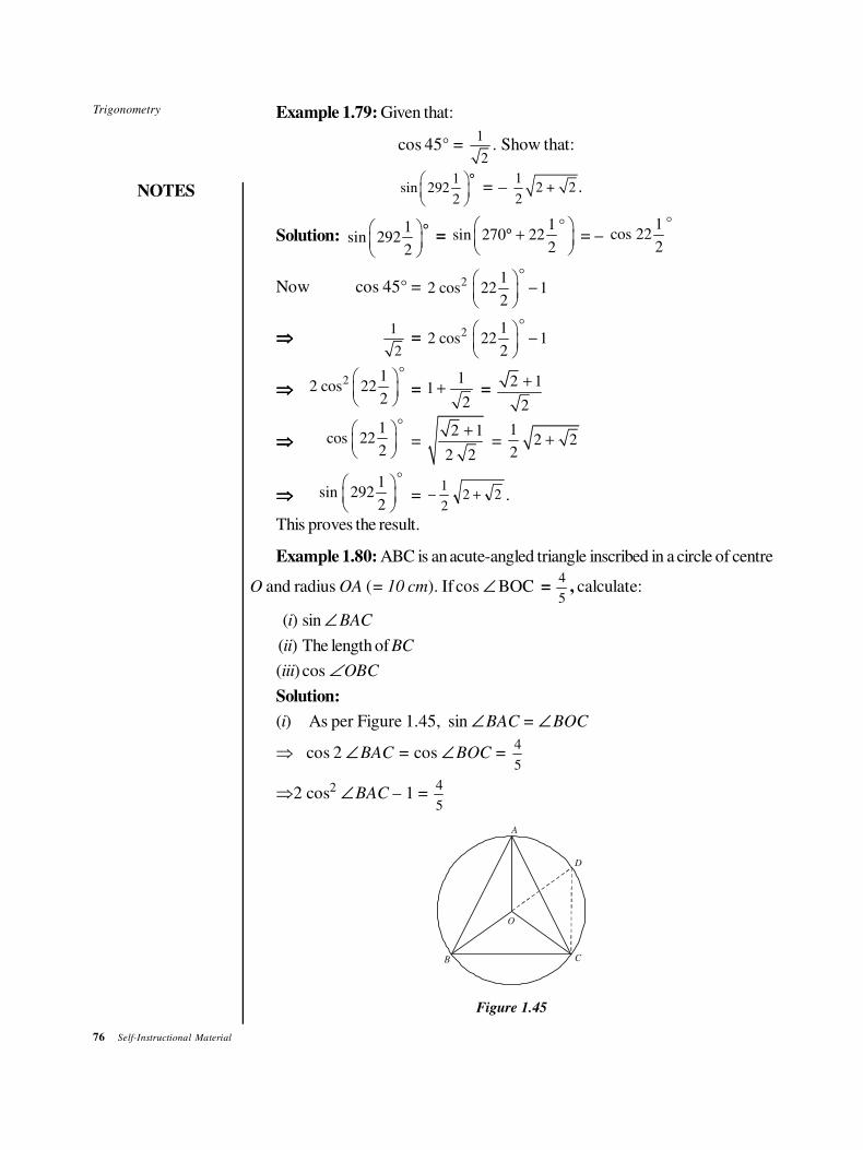
76 Self-Instructional Material
Trigonometry
NOTES
Example 1.79: Given that:
cos 45° = 1
2. Show that:
1sin 292
2
°
= – 1
2 + 22
.
Solution: 1
sin 2922
°
= 1 °
sin 270 222
° +
= –
°1cos 22
2
Now cos 45° = 2°1
2 cos 22 12
−
⇒⇒⇒⇒1
2= 2
°12 cos 22 1
2
−
⇒⇒⇒⇒2
°12 cos 22
2
= 1
12
+ = 2 1
2
+
⇒⇒⇒⇒°1
cos 222
= 2 1
2 2
+ =
12 2
2+
⇒⇒⇒⇒°1
sin 2922
= 222
1+− .
This proves the result.
Example 1.80: ABC is an acute-angled triangle inscribed in a circle of centre
O and radius OA (= 10 cm). If cos ∠ BOC = 5
4, calculate:
(i) sin ∠BAC
(ii) The length of BC
(iii) cos ∠OBC
Solution:
(i) As per Figure 1.45, sin ∠BAC = ∠BOC
⇒ cos 2 ∠BAC = cos ∠BOC = 4
5
⇒2 cos2 ∠BAC – 1 = 4
5
D
O
CB
A
Figure 1.45
Trigonometry
NOTES
Self-Instructional Material 77
⇒ 2 cos2 ∠BAC = 9
5
⇒ cos2 ∠BAC = 9
10
⇒ sin2∠BAC = 1 – 9
10 =
1
10
⇒ sin ∠BAC = 1
10(as BAC is an acute angle).
(ii) Produce BO to meet the circle at D and join CD.
Then, BCD is a right angle (angle in a semi-circle). Also, ∠BDC
= ∠BAC (angles in same segment).
So, sin ∠BDC = BC
BD =
20
BC
⇒ sin ∠BAC = 20
BC
⇒1
10=
20
BC ⇒ BC =20
10 = 2 10 .
(iii) cos ∠OBC = cos (90° – ∠BDC) = cos (90° – ∠BAC)
= sin ∠BAC = 1
10.
Example 1.81: If tan A tan 2A ≠ – 1 prove that:
tan 3A tan 2A tan A = tan 3A – tan 2A – tan A.
Solution: Now, tan 3A tan 2A tan A – tan 3A
= tan 3A (tan 2A tan A – 1)
= tan (2A + A) (tan 2A tan A – 1)
= tan 2 tan
1 tan tan 2
A A
A A
+
− (tan A tan 2A – 1)
= – (tan 2A + tan A)
This proves the result.
Example 1.82: Prove that:
1 sin cos
1 sin cos
A A
A A
+ −
+ + = tan
A
2
Solution: LHS = (1 cos ) sin
(1 cos ) sin
A A
A A
− +
+ +
=
2
2
2 sin 2 sin cos2 2 2
2 cos 2 sin cos2 2 2
A A A
A A A
+
+
=
2 sin sin cos2 2 2
2 cos sin cos2 2 2
A A A
A A A
+
+
= tan2
A
78 Self-Instructional Material
Trigonometry
NOTES
Example 1.83: If tan x = 1 cos
sin
y
y
−, then prove that one of the solutions will
be y = 2x. Use this result to prove that 1
tan 72
° = 6 – 3 + 2 – 2 .
Solution: Now, 1 cos
sin
y
y
− =
1 cos 2
sin 2
x
x
− =
22 sin
2 sin cos
x
x x = tan x
⇒ y = 2x is one of the solution.
Thus,1
tan 72
°=
1 cos15
sin15
− °
°
But cos 15° = cos (45 – 30) = 3 1 1 1
2 22 2+ =
3 1
2 2
+
and sin 15° = sin (45 – 30) = 1 3 1 1
2̀ 22 2− =
3 1
2 2
−
⇒1
tan 72
°=
3 11
2 2
3 1
2 2
+−
− =
2 2 3 1
3 1
− −
−
= (2 2 3 1) ( 3 1)
2
− − +
=2 6 2 3 2 2 4
2
− + −= 6 3 2 2− + −
Example 1.84: Prove that:
π1 cos
8
+
3π1 cos
8
+
5π1 cos
8
+
7π1 + cos
8
= 1
8
Solution: Now, 3
cos8
π = cos
2 8
π π −
= sin
8
π−
5πcos
8=
π πcos
2 8
+
=
πsin
8−
7πcos
8=
πcos
8
π −
= π
cos8
−
LHS = π
1 cos8
+
π1 sin
8
+
π1 sin
8
−
π1 cos
8
−
= 2 π1 cos
8
−
2 π1 sin8
−
= 2 2π π
sin cos8 8
=
21 π π
2 sin cos4 8 8
=
21 π
sin4 4
=
21 1
4 2
= 1
8 = RHS.
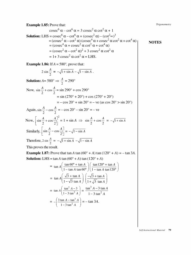
Trigonometry
NOTES
Self-Instructional Material 79
Example 1.85: Prove that:
cosec6 α – cot6 α = 3 cosec2
α cot2 α + 1
Solution: LHS = cosec6 α – cot6 α = (cosec2 α) – (cot2∝)3
= (cosec2 α – cot2 α) (cosec4 α + cosec2 α cot2 α + cot4 α)
= (cosec4 α + cosec2 α cot2 α + cot4 α)
= (cosec2 α – cot2 α)2 + 3 cosec2 α cot2 α
= 1+ 3 cosec2 α cot2 α = LHS.
Example 1.86: If A = 580°, prove that:
2 sin2
A= 1 sin 1 sinA A− + − − .
Solution: A= 580° ⇒ 2
A = 290°
Now, sin cos2 2
A A+ = sin 290° + cos 290°
= sin (270° + 20°) + cos (270° + 20°)
= – cos 20° + sin 20° = – ve (as cos 20° > sin 20°)
Again, sin cos2 2
A A− = – cos 20° – sin 20° = – ve
Now, 2
sin cos2 2
A A +
= 1 + sin A ⇒ sin cos
2 2
A A+ = 1 sin A− +
Similarly, sin cos2 2
A A −
= 1 sin A− −
Therefore,2
sin2A
= 1 sin A− + 1 sin A− −
This proves the result.
Example 1.87: Prove that tan A tan (60° + A) tan (120° + A) = – tan 3A.
Solution: LHS = tan A tan (60° + A) tan (120° + A)
= tan 60 tantan
1 tan tan 60
AA
A
° +
− °
tan120 tan
1 tan tan120
A
A
° +
− °
= 3 tan
tan1 3 tan
AA
A
+ −
3 tan
1 3 tan
A
A
− + +
=
−
−
A
AA
2
2
tan31
3tantan =
3
2
tan 3 tan
1 3 tan
A A
A
−
−
=
−
−−
A
AA
2
3
tan31
tantan3 = – tan 3A.
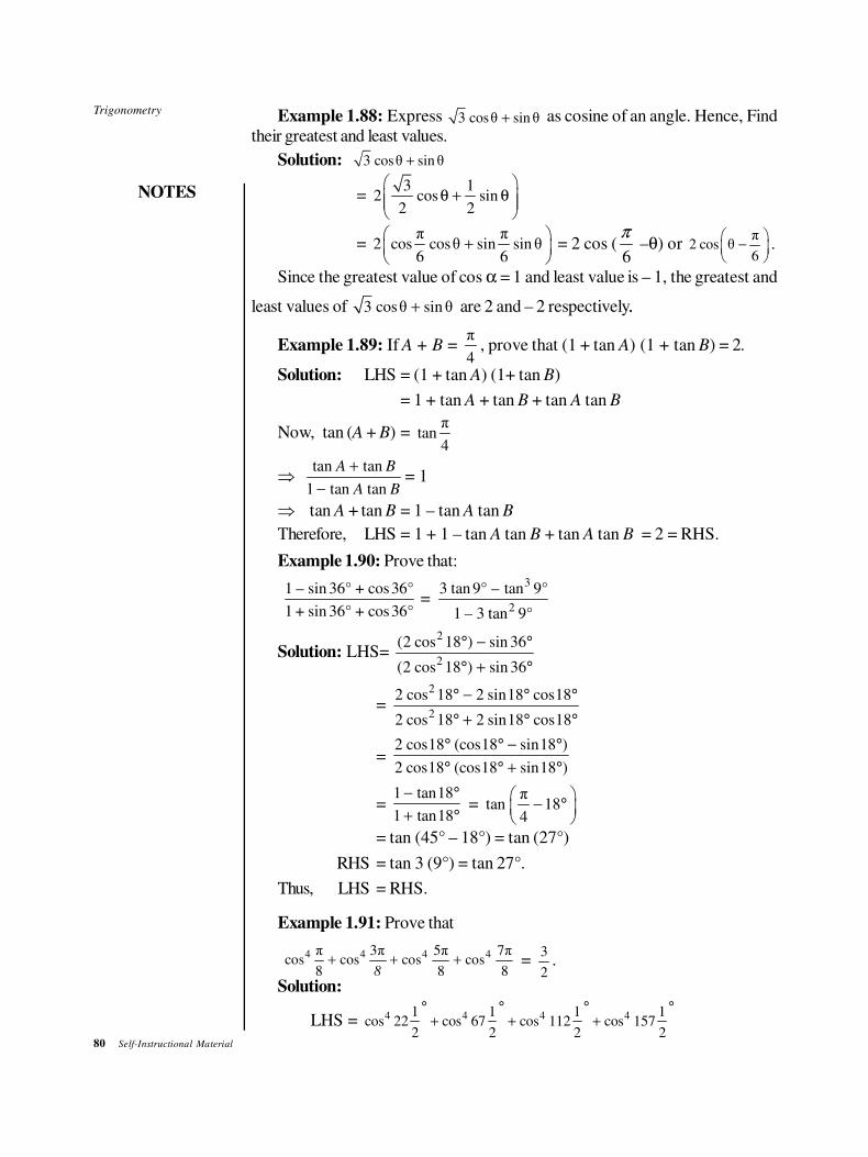
80 Self-Instructional Material
Trigonometry
NOTES
Example 1.88: Express 3 cosθ sinθ+ as cosine of an angle. Hence, Find
their greatest and least values.
Solution: 3 cosθ sinθ+
= 3 1
2 cos sin2 2
θ + θ
= π π
2 cos cosθ sin sinθ6 6
+
= 2 cos (
6
π –θ) or
π2 cos θ
6
−
.
Since the greatest value of cos α = 1 and least value is – 1, the greatest and
least values of 3 cosθ sinθ+ are 2 and – 2 respectively..
Example 1.89: If A + B = π
4, prove that (1 + tan A) (1 + tan B) = 2.
Solution: LHS = (1 + tan A) (1+ tan B)
= 1 + tan A + tan B + tan A tan B
Now, tan (A + B) = π
tan4
⇒ tan tan
1 tan tan
A B
A B
+
−= 1
⇒ tan A + tan B = 1 – tan A tan B
Therefore, LHS = 1 + 1 – tan A tan B + tan A tan B = 2 = RHS.
Example 1.90: Prove that:
1 – sin 36° + cos36°
1 + sin 36° + cos36° =
3
2
3 tan 9° – tan 9°
1 – 3 tan 9°
Solution: LHS= 2
2
(2 cos 18 ) sin 36
(2 cos 18 ) sin 36
° − °
° + °
= 2
2
2 cos 18 2 sin18 cos18
2 cos 18 2 sin18 cos18
° − ° °
° + ° °
= 2 cos18 (cos18 sin18 )
2 cos18 (cos18 sin18 )
° ° − °
° ° + °
= 1 tan18
1 tan18
− °
+ ° =
πtan 18
4
− °
= tan (45° – 18°) = tan (27°)
RHS = tan 3 (9°) = tan 27°.
Thus, LHS = RHS.
Example 1.91: Prove that
4 4 4 4π 3π 5π 7π
cos cos cos cos8 8 88
+ + + = 3
2.
Solution:
LHS = 4 4 4 41 1 1 1cos 22 cos 67 cos 112 cos 157
2 2 2 2
° ° ° °+ + +
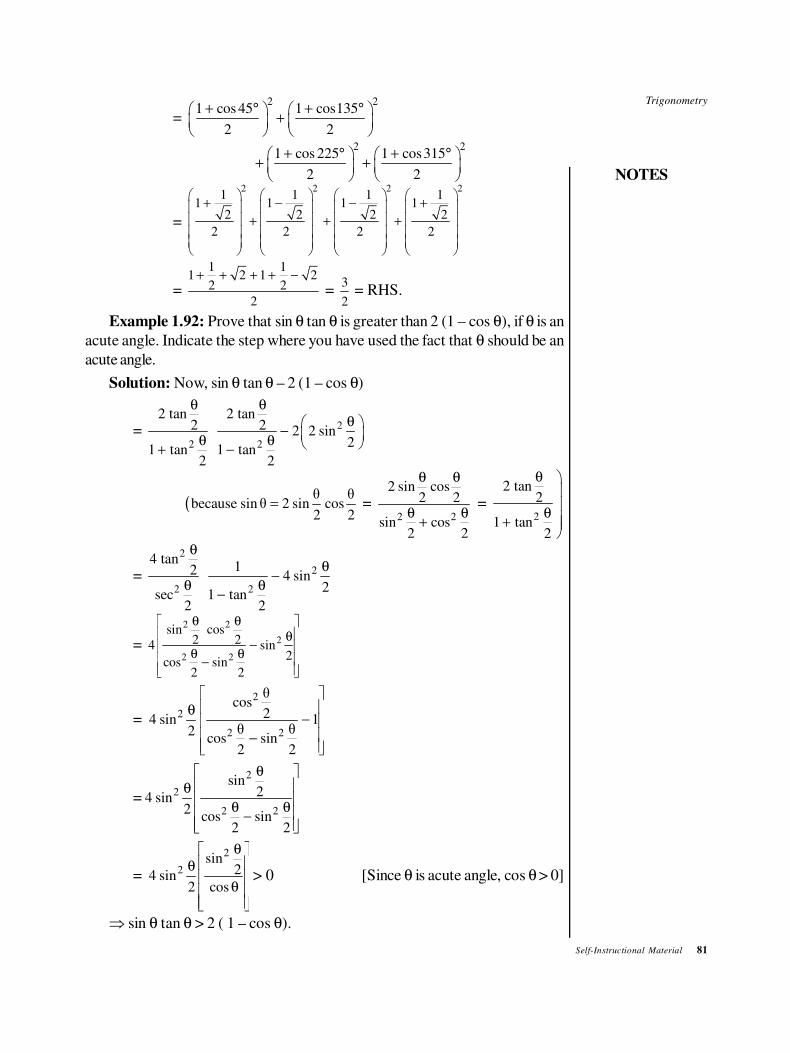
Trigonometry
NOTES
Self-Instructional Material 81
= 2 2
1 cos 45 1 cos135
2 2
+ ° + ° +
2 2
1 cos 225 1 cos315
2 2
+ ° + ° + +
=
2 21 1
1 12 2
2 2
+ −
+
2 21 1
1 12 2
2 2
− +
+ +
=
1 11 2 1 2
2 2
2
+ + + + − =
3
2 = RHS.
Example 1.92: Prove that sin θ tan θ is greater than 2 (1 – cos θ), if θ is an
acute angle. Indicate the step where you have used the fact that θ should be an
acute angle.
Solution: Now, sin θ tan θ – 2 (1 – cos θ)
= 2
2 2
2 tan 2 tan2 2 2 2 sin
21 tan 1 tan
2 2
θ θθ
− θ θ + −
(θ θ
because sin θ 2 sin cos2 2
= = 2 2
2 sin cos2 2
sin cos2 2
θ θ
θ θ+
= 2
2 tan2
1 tan2
θ
θ +
=
2
2
2 2
4 tan12 4 sin
2sec 1 tan
2 2
θθ
−θ θ
−
=
2 2
2
2 2
sin cos2 24 sin
2cos sin
2 2
θ θ θ
− θ θ −
=
2
2
2 2
θcos
24 sin 1θ θ2
cos sin2 2
θ
− −
=
2
2
2 2
sin24 sin
2cos sin
2 2
θ θ θ θ −
=
2
2sin
24 sin 02 cos
θ θ
θ
> 0 [Since θ is acute angle, cos θ > 0]
⇒ sin θ tan θ > 2 ( 1 – cos θ).
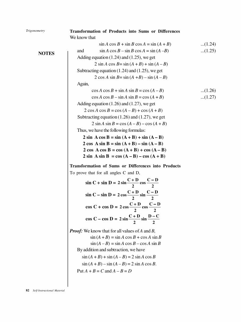
82 Self-Instructional Material
Trigonometry
NOTES
Transformation of Products into Sums or Differences
We know that
sin A cos B + sin B cos A = sin (A + B) ...(1.24)
and sin A cos B – sin B cos A = sin (A –B) ...(1.25)
Adding equation (1.24) and (1.25), we get
2 sin A cos B= sin (A + B) + sin (A – B)
Subtracting equation (1.24) and (1.25), we get
2 cos A sin B= sin (A +B) – sin (A – B)
Again,
cos A cos B + sin A sin B = cos (A – B) ...(1.26)
cos A cos B – sin A sin B = cos (A + B) ...(1.27)
Adding equation (1.26) and (1.27), we get
2 cos A cos B = cos (A – B) + cos (A + B)
Subtracting equation (1.26) and (1.27), we get
2 sin A sin B = cos (A – B) – cos (A + B)
Thus, we have the following formulas:
2 sin A cos B = sin (A + B) + sin (A – B)
2 cos A sin B = sin (A + B) – sin (A – B)
2 cos A cos B = cos (A + B) + cos (A – B)
2 sin A sin B = cos (A – B) – cos (A + B)
Transformation of Sums or Differences into Products
To prove that for all angles C and D,
sin C + sin D = C + D C D
2 sin cos2 2
−−−−
sin C – sin D = C + D C D
2 cos sin2 2
−−−−
cos C + cos D = C + D C D
2 cos cos2 2
−−−−
cos C – cos D = C + D D C
2 sin sin2 2
−−−−
Proof: We know that for all values of A and B,
sin (A + B) = sin A cos B + cos A sin B
sin (A – B) = sin A cos B – cos A sin B
By addition and subtraction, we have
sin (A + B) + sin (A – B) = 2 sin A cos B
sin (A + B) – sin (A – B) = 2 sin A cos B.
Put A + B = C and A – B = D
Trigonometry
NOTES
Self-Instructional Material 83
We get 2
C DA
+= ,
2
C DB
−= .
Then, sin C + sin D = 2 sin cos2 2
C D C D+ −
sin C – sin D = 2 cos sin2 2
C D C D+ −.
Similarly, by adding and subtracting the relations,
cos (A + B) = cos A cos B – sin A sin B
cos (A – B) = cos A cos B + sin A sin B.
We have,
cos (A + B) + cos (A – B) = 2 cos A cos B
cos (A + B) – cos (A – B) = – 2 sin A sin B.
Put A + B = C, A – B = D
So that2
C DA
+= ,
2
C DB
−= .
Hence, cos C + cos D = 2 cos cos2 2
C D C D+ −
cos C – cos D = 2 sin sin2 2
C D C D+ −−
= 2 sin sin2 2
C D D C+ −.
To prove that,
(i) sin (A + B) sin (A – B) = sin2 A – sin2 B
(ii) cos (A + B) cos (A – B) = cos2 A – sin2 B = cos2 B – sin2 A
Proof: (i) sin (A + B) sin (A – B)
= (sin A cos B + cos A sin B) (sin A cos B – cos A sin B)
= sin2 A cos2 B – cos2 A sin2 B
= sin2 A (1 – sin2 B) – (1 – sin2 A) sin2 B
= sin2 A – sin2 A sin2 B – sin2 B + sin2 A sin2 B
= sin2 A – sin2 B.
(ii) cos (A + B) cos (A – B).
= (cos A cos B – sin A sin B) (cos A cos B + sin A sin B)
= cos2 A cos2 B – sin2 A sin2 B
= cos2 A (1 – sin2 B) – (1 – cos2 A) sin2 B
= cos2 A – cos2 A sin2 B – sin2 B + cos2 A sin2 B
= cos2 A – sin2 B
= (1– sin2 A) – (1 – cos2 B)
= cos2 B – sin2 A
84 Self-Instructional Material
Trigonometry
NOTES
Example 1.93: If the angles A, B, C, of a triangle are in A.P, show that:
cos cos
sin sin
C A
A C
−
−= tan B.
Solution: Since in any triangleA + B + C = π
and C = π–(A + B)cos C = – cos (A + B)
and sin C = sin (A + B)
LHS = cos ( ) cos
sin sin ( )
A B A
A A B
− + −
− +
=
2 cos cos2 2
2 cos sin2 2
B BA
B BA
− +
− +
= π
cot cot2 2 2
B A C + = −
= tan2
A C+
= tan B
As , , are in A.P.2
A CA B C B
+ ⇒ =
Example 1.94 Prove that:2 2sin – sin
sin cos – sin cos
A B
A A B B = tan (A + B).
Solution: LHS = 2 2
2 sin ( ) sin ( )
sin sin
A B A B
A B
+ −
−
= 2 sin ( ) sin ( )
2 cos ( ) sin ( )
A B A B
A B A B
+ −
+ − = tan (A + B) = RHS.
Example 1.95: Prove that 4 (cos3 10° + sin3
20°) = 3 (cos 10° + sin 20°).
Solution: LHS= 4 (cos 10° + sin 20°) (cos2 10° + sin2 20°
+ cos 10° sin 20°)
= 4 (cos 10° + sin 20°) (1 – sin2 10° + sin2 20°
+ cos 10° sin 20°)
= 4 (cos 10° + sin 20°) (1 + sin 30° sin 10°
– cos 10° sin 20°)
= 4 (cos 10° + sin 20°) sin10º
12
+
(sin 30º sin10º )
2
+ −
.
= 2 (cos 10° + sin 20°) 1
2 sin10 sin102
+ ° − − °
= 2 (cos 10° + sin 20°) 3
2
= 3 (cos 10° + sin 20°) = RHS.
Trigonometry
NOTES
Self-Instructional Material 85
Example 1.96: Given x = cos 55°, y = cos 65°
z = cos 175°. Prove that:
x + y + z = 0 and xy + yz + zx = 3
-4
.
Solution: x + y + z = cos 55° + cos 65° + cos 175°
= 2 cos 60° cos 5° + cos (180° – 5°)
= cos 5° – cos 5° = 0.
xy + yz + zx = cos 55° cos 65° + cos 65° cos 175° + cos 175° cos 55°
= 1
2 (cos 120° + cos 10°) +
1
2 (cos 240° + cos 110°)
+ 1
2 (cos 230° + cos 120°)
= – 1
4 +
1
2 cos 10° –
1
4 +
1
2 cos 110°10°
+ 1
2 cos 230° –
1
4
= – 3
4 +
1
2 [cos 10° + cos 110° + cos 230°]
= – 3
4 +
1
2 [2 cos 60° cos 50° – cos 50°]
= – 3
4 +
1
2 [cos 50° – cos 50°] = –
3
4 .
Example 1.97: Prove that:
sin2 B = sin2
A + sin2 (A – B) – 2 sin A cos B sin (A – B).
Solution: RHS= sin2 A + sin2 (A – B) – (2 sin A cos B) sin (A – B)
= sin2 A + sin2 (A – B) – [sin (A + B)
+ sin (A – B)] × sin (A – B)
= sin2 A + sin2 (A – B) – sin (A + B)
sin (A – B) – sin2 (A – B)
= sin2 A – sin (A + B) sin (A – B)
= sin2 A – (sin2 A – sin2 B)
= sin2 B = LHS.
Example 1.98: If y sin α = x sin (2β + α)
show that (x + y) cot (α + β) = (y – x) cot β.
Solution: y sin α= x sin (2β + α)
⇒y
x=
sin (2β )
sin
+ α
α
Applying componendo and dividendo
86 Self-Instructional Material
Trigonometry
NOTES
⇒y x
y x
+
− =
sin (2β α) sin α
sin (2β α) sinα
+ +
+ −
⇒y x
y x
+
−=
2sin (α β) cosβ
2cos (α β) sin β
+
+⇒
y x
y x
+
− = tan (α + β) cot β
⇒ (y + x) cot (α + β) = (y – x) cot β
This proves the result.
Example 1.99: Prove that:
cos cos sin sin
sin sin cos cos
n n
A B A B
A B A B
+ ++
− −
= cotn A B2
2
−
or 0 according as n is even or odd.
Solution:
nn
BA
BA
BA
BA
−
++
−
+
coscos
sinsin
sinsin
coscos
=2 cos cos 2 sin cos
2 2 2 2
2 sin cos 2 sin sin2 2 2 2
n nA B A B A B A B
A B A B A B B A
+ − + −
+ − + + −
=( ) ( )
cot cot2 2
n nA B A B− −
+ −
So, LHS = 2 cot2
n A B−
if n is even and 0 if n is odd.
Example 1.100: If sin x + sin y = a and cos x + cos y = b show that
cos (x + y) =
2 2
2 2
b a
b a
−
+
Solution: Now, sin x + sin y = a
⇒ 2 sin cos2 2
x y x y+ −= a
and cos x + cos y = b
⇒ 2 cos cos2 2
x y x y+ −= b
Therefore, tan2
x y+
= a
b
Now, cos (x + y) =
2
2
1 tan2
1 tan2
x y
x y
+ −
+ +
=
2
2
2
2
1
1
a
b
a
b
−
+
= 2 2
2 2
b a
b a
−
+.
Example 1.101: Prove that in a triangle ABC:
sin (A – B) sin (B – C) sin (C – A)+ +
sin A sin B sin B sin C sin C sin A = 0.
Trigonometry
NOTES
Self-Instructional Material 87
Solution: LHS = sin sin ( ) sin sin ( ) sin sin ( )
sin sin sin
C A B A B C B C A
A B C
− + − + −
=
sin ( ) sin ( ) sin ( ) sin ( )
sin ( ) sin ( )
sin sin sin
A B A B B C B C
C A C A
A B C
++ − + −+ + −
(Using A + B + C = π)
= 2 2 2 2 2 2
(sin sin ) (sin sin ) (sin sin )
sin sin sin
A B B C C A
A B C
− + − + −
= 0 = RHS.
Example 1.102: Prove that, 1 + cos 56° + cos 58° – cos 66°
= 4 cos 28° cos 29° sin 33°
Solution: Now, 1 – cos 66° = 2 sin2 33°.
Therefore, LHS = 2 sin2 33° + (cos 56° + cos 58°)
= 2 sin2 33° + 2 cos 57° cos 1°
= 2 sin2 33° + 2 cos (90° – 33°) cos 1°
= 2 sin2 33° + 2 sin 33° cos 1°
= 2 sin 33° (sin 33° + cos 1°)
= 2 sin 33° (cos 57° + cos 1°)
= 2 sin 33° (2 cos 29°cos 28°)
= 4 cos 28° cos 29° sin 33° = RHS.
Example 1.103: Prove that sin2 12° + sin2 21° + sin2 39° + sin2 48°
= 1 + sin2 9° + sin2 18°.
Solution: Consider
(sin2 12° – sin2 18°) + (sin2 21° – sin 9°)
= (– sin 30° sin 6°) + (sin 30° sin 12°)
= sin 30° (sin 12° – sin 6°)
= 1
2 (2 sin 3° cos 9°) = sin 3° cos 9°
Also,1 – sin2 39° – sin2 48° = cos2 39° – sin2 48°
= cos 87° cos 9° = sin 3° cos 9°
Therefore, (sin2 12° – sin2 18°) + (sin2 21° – sin2 9°)
= 1 – sin2 39° – sin2 48°.
The proves the result.
Example 1.104: Prove that cos 10° cos 50° cos 70° = 3
8.
Solution: LHS = cos 10° cos 50° cos 70°
= cos 10° 1
(cos120º cos 20º )2
+
88 Self-Instructional Material
Trigonometry
NOTES
= 1
2 cos 10°
1cos 20º
2
− +
= 1
2 cos 10° 21
2cos 10º 12
− + −
= 1
2 cos 10° 23
2 cos 102
− + °
= 1
4 cos 10° (4 cos2 10° – 3)
= 1
4(4 cos3 10° – 3 cos 10°)
= 1
4 cos 3 × 10° =
1
4 cos 30°
= 1 3
4 2 =
3
8 = RHS.
Example 1.105: If A + B + C = π, then prove that:
tan A + tan B + tan C = tan A tan B tan C.
Solution: A + B + C = π
⇒ A + B = π – C
⇒ tan (A + B ) = – tan C
⇒tan tan
1 tan tan
A B
A B
+
−= – tan C
⇒tan A + tan B + tan C = tan A tan B tan C
This proves the result.
Example 1.106: If A + B + C = π, then prove that:
2 2 2sin sin sin
2 2 2
A B C+ + = 1 2
2 2 2
A B Csin sin sin− .
Solution: Consider,
2 2 21 sin sin sin
2 2 2
A B C− − − = 2 2 2
cos sin sin2 2 2
A B C− −
= 2cos cos sin
2 2 2
A B A B C+ − −
= 2
cos cos cos2 2 2
A B A B A B+ − + −
as
2
C
= π
2 2
A B+ −
= cos cos cos2 2 2
A B A B A B+ − + −
= cos 2 sin sin2 2 2
A B A B+
= 2 sin sin sin2 2 2
A B C
Trigonometry
NOTES
Self-Instructional Material 89
Hence, 2 2 2sin sin sin2 2 2
A B C+ + = 1 2 sin sin sin
2 2 2
A B C− .
Example 1.107: If A + B + C = π, prove that:
cos2 A + cos2
B + cos2 C = 1 – 2 cos A cos B cos C.
Solution: Consider 1 – (cos2 A + cos2 B + cos2 C)
= (1 – cos2 A) – cos2 B – cos2 C
= sin2 A – cos2 B – cos2 C
= – cos (A + B) cos (A – B) – cos2 C
= – cos (π – C) cos (A – B) – cos2 C
= cos C cos (A – B) – cos2 C
= cos C [cos (A – B) – cos C]
= cos C [cos (A – B) – cos (π – (A + B)]
= cos C [cos (A – B) + cos (A + B)]
= cos C [2 cos A cos B]
= 2 cos A cos B cos C
Thus, cos2A + cos2B + cos2C = 1 – 2cosA cosB cosC
This proves the result.
CHECK YOUR PROGRESS
17. Prove that sin 105° + cos 105° = cos 45°.
18. Find the value of tan 75° and hence prove that tan 75° + cot 75° = 4.
19. Prove that cos13° + sin13°
cos13° – sin13° = tan 58°.
20. Prove that °1
cot 222
– °1
tan 222
= 2
21. Prove that cos A + sin A
1 + sin 2A = 1.
22. If, A + B + C = π, show that
sin 2A + sin 2B – sin 2C = 4 cos A cos B sin C.
23. In a ∆ ABC, prove that
sin 2A + sin 2B + sin 2C = 4 sin A sin B sin C.
1.9 SUMMARY
In this unit, you have learned that:
• Trigonometry is that branch of mathematics which deals with the
measurement of angles.
90 Self-Instructional Material
Trigonometry
NOTES
• The term ‘trigonometry’ is derived from two Greek words ‘trigonon’ (a
triangle) and ‘metron’ (a measure), meaning the measurement of triangles.
• Nowadays, the term trigonometry is used for the measurement of angles in
general, whether the angles are of a triangle or not.
• An angle is defined as the rotation of a line about one of its extremities in a
plane from one position to another.
• Two lines are said to be at right angles, if a revolving line starting from one
position to another describes one-quarter of a circle.
• When a revolving line moves in the anticlockwise direction, the angle
described by it is said to be positive; otherwise, it is called negative.
• To measure angles, a particular angle is fixed and is taken as a unit of
measurement so that any other angle is measured by the number of times it
contains that unit.
• There are three systems of measurement:
(i) Sexagesimal system: In this system, a right angle is divided into 90 equal
parts called degrees. Each degree is divided into 60 equal parts called
minutes and each minute is further subdivided into 60 equal parts called
seconds.
Thus, 1 right angle =90 degrees
1 degree =60 minutes
1 minute =60 seconds
In symbols, a degree, a minute and a second are respectively written as 1º;
1′, 1′′.
(ii) Centesimal system: In this system, a right angle is divided into 100 equal
parts called grades. Each grade is divided into 100 equal parts called
minutes and each minute is divided into 100 equal parts called seconds.
Thus, 1 right angle = 100 grades
1 grade = 100 minutes
1 minute = 100 seconds
(iii) Circular system: In this system, the unit of measurement is radian. A
radian is defined as the angle subtended at the centre of a circle by an
arc equal to the radius of the circle.
• Trigonometry deals with the problem of measurement of triangles and periodic
functions.
• The applications of trigonometry to business cycles and other situations are
concerned with the properties and applications of circular or periodic
functions.
• A function with period p(p ≠ 0) if f(x + p) = f(x) is periodic.
• The amplitude of a sine wave is the absolute value of one half of the difference
between the greatest and the least ordinates of the wave.
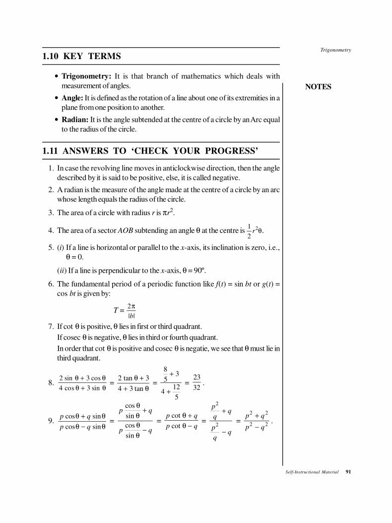
Trigonometry
NOTES
Self-Instructional Material 91
1.10 KEY TERMS
• Trigonometry: It is that branch of mathematics which deals with
measurement of angles.
• Angle: It is defined as the rotation of a line about one of its extremities in a
plane from one position to another.
• Radian: It is the angle subtended at the centre of a circle by an Arc equal
to the radius of the circle.
1.11 ANSWERS TO ‘CHECK YOUR PROGRESS’
1. In case the revolving line moves in anticlockwise direction, then the angle
described by it is said to be positive, else, it is called negative.
2. A radian is the measure of the angle made at the centre of a circle by an arc
whose length equals the radius of the circle.
3. The area of a circle with radius r is πr2.
4. The area of a sector AOB subtending an angle θ at the centre is 1
2
2r θ.
5. (i) If a line is horizontal or parallel to the x-axis, its inclination is zero, i.e.,
θ = 0.
(ii) If a line is perpendicular to the x-axis, θ = 90º.
6. The fundamental period of a periodic function like f(t) = sin bt or g(t) =
cos bt is given by:
T = 2π
| |b
7. If cot θ is positive, θ lies in first or third quadrant.
If cosec θ is negative, θ lies in third or fourth quadrant.
In order that cot θ is positive and cosec θ is negatie, we see that θ must lie in
third quadrant.
8.2 3
4 3
sin cos
cos sin
θ θ
θ θ
+
+ =
2 3
4 3
tan
tan
θ
θ
+
+ =
8
53
412
5
+
+ =
23
32.
9.p q
p q
cos sin
cos sin
θ θ
θ θ
+
− =
p q
p q
cos
sin
cos
sin
θ
θ
θ
θ
+
−
= p q
p q
cot
cot
θ
θ
+
− =
p
p
2
2
+
−
= p q
p q
2 2
2 2
+
−.
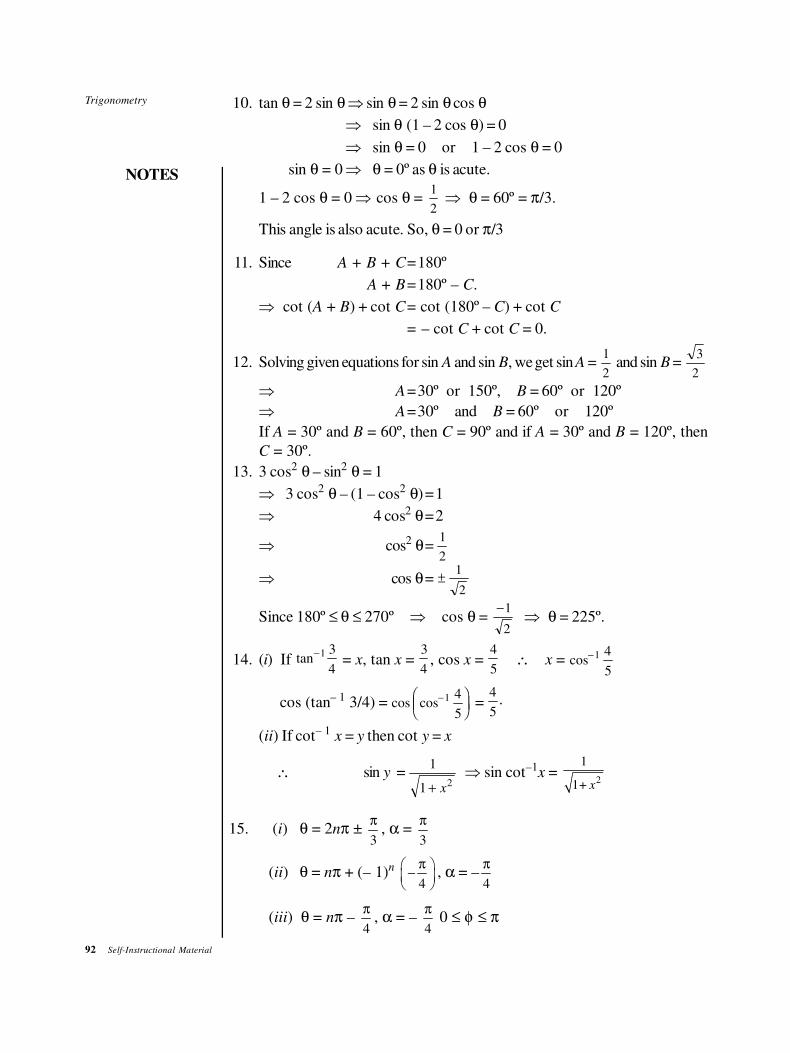
92 Self-Instructional Material
Trigonometry
NOTES
10. tan θ = 2 sin θ ⇒ sin θ = 2 sin θ cos θ
⇒ sin θ (1 – 2 cos θ) = 0
⇒ sin θ = 0 or 1 – 2 cos θ = 0
sin θ = 0⇒ θ = 0º as θ is acute.
1 – 2 cos θ = 0 ⇒ cos θ = 1
2 ⇒ θ = 60º = π/3.
This angle is also acute. So, θ = 0 or π/3
11. Since A + B + C=180º
A + B=180º – C.
⇒ cot (A + B) + cot C= cot (180º – C) + cot C
= – cot C + cot C = 0.
12. Solving given equations for sin A and sin B, we get sin A = 1
2 and sin B =
3
2
⇒ A=30º or 150º, B = 60º or 120º
⇒ A=30º and B = 60º or 120º
If A = 30º and B = 60º, then C = 90º and if A = 30º and B = 120º, then
C = 30º.
13. 3 cos2 θ – sin2 θ = 1
⇒ 3 cos2 θ – (1 – cos2 θ)=1
⇒ 4 cos2 θ=2
⇒ cos2 θ=1
2
⇒ cos θ= ±1
2
Since 180º ≤ θ ≤ 270º ⇒ cos θ = −1
2⇒ θ = 225º.
14. (i) If tan−1 3
4 = x, tan x =
3
4, cos x =
4
5∴ x = cos−1 4
5
cos (tan– 1 3/4) = cos cos−FHG
IKJ
1 4
5 =
4
5.
(ii) If cot– 1x = y then cot y = x
∴ sin y =1
1 2+ x
⇒ sin cot–1x =
2
1
1+ x
15. (i) θ = 2nπ ± 3
π, α =
3
π
(ii) θ = nπ + (– 1)n 4
π −
, α = –4
π
(iii) θ = nπ – 4
π, α = –
4
π 0 ≤ φ ≤ π
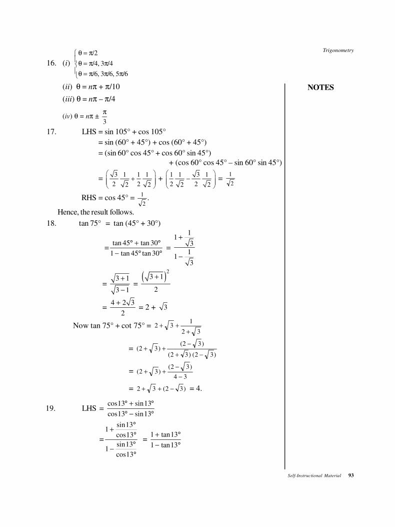
Trigonometry
NOTES
Self-Instructional Material 93
16. (i) /4, 3 /4
/6, 3 /6, 5 /6
θ = π/2
θ = π πθ = π π π
(ii) θ = nπ + π/10
(iii) θ = nπ – π/4
(iv) θ = nπ ± 3
π
17. LHS = sin 105° + cos 105°
= sin (60° + 45°) + cos (60° + 45°)
= (sin 60° cos 45° + cos 60° sin 45°)
+ (cos 60° cos 45° – sin 60° sin 45°)
= 3 1 1 1
2 22 2
+
+
1 1 3 1
2 22 2
−
=
2
1
RHS = cos 45° = 2
1.
Hence, the result follows.
18. tan 75° = tan (45° + 30°)
=tan 45 tan 30
1 tan 45 tan 30
° + °
− ° ° =
11
3
11
3
+
−
= 3 1
3 1
+
− =
( )2
3 1
2
+
= 4 2 3
2
+ = 2 + 3
Now tan 75° + cot 75° =32
132
+++
= )32()32(
)32()32(
−+
−++
= 34
)32()32(
−
−++
= )32(32 −++ = 4.
19. LHS = cos13 sin13
cos13 sin13
° + °
° − °
=
sin131
cos13
sin131
cos13
°+
°
°−
°
= 1 tan13
1 tan13
+ °
− °
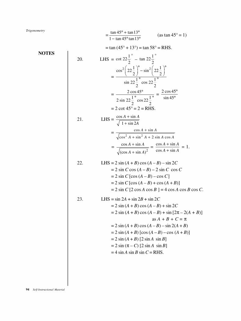
94 Self-Instructional Material
Trigonometry
NOTES
=tan 45 tan13
1 tan 45 tan13
° + °
− ° °(as tan 45° = 1)
= tan (45° + 13°) = tan 58° = RHS.
20. LHS = °1
cot 222
– °1
tan 222
=
2 21 1cos 22 sin 22
2 2
1 1sin 22 cos 22
2 2
° ° −
° °
= 2 cos 45
1 12 sin 22 cos 22
2 2
°
° ° =
2 cos 45
sin 45
°
°
= 2 cot 45° = 2 = RHS.
21. LHS = cos sin
1 sin 2
A A
A
+
+
= 2 2
cos sin
cos sin 2 sin cos
A A
A A A A
+
+ +
= 2
cos sin
(cos sin )
A A
A A
+
+=
cos sin
cos sin
A A
A A
+
+ = 1.
22. LHS = 2 sin (A + B) cos (A – B) – sin 2C
= 2 sin C cos (A – B) – 2 sin C cos C
= 2 sin C [cos (A – B) – cos C]
= 2 sin C [cos (A – B) + cos (A + B)]
= 2 sin C [2 cos A cos B ] = 4 cos A cos B cos C.
23. LHS = sin 2A + sin 2B + sin 2C
= 2 sin (A + B) cos (A – B) + sin 2C
= 2 sin (A + B) cos (A – B) + sin [2π – 2(A + B)]
as A + B + C = π
= 2 sin (A + B) cos (A – B) – sin 2(A + B)
= 2 sin (A + B) [cos (A – B) – cos (A + B)]
= 2 sin (A + B) [2 sin A sin B]
= 2 sin (π – C) [2 sin A sin B]
= 4 sin A sin B sin C = RHS.
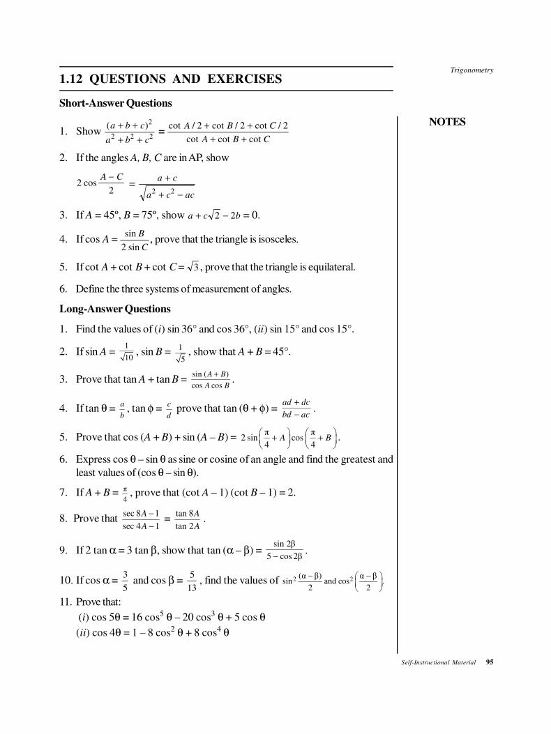
Trigonometry
NOTES
Self-Instructional Material 95
1.12 QUESTIONS AND EXERCISES
Short-Answer Questions
1. Show ( )a b c
a b c
+ +
+ +
2
2 2 2 =
cot / cot / cot /
cot cot cot
A B C
A B C
2 2 2+ +
+ +
2. If the angles A, B, C are in AP, show
22
cosA C−
= a c
a c ac
+
+ −2 2
3. If A = 45º, B = 75º, show a c b+ −2 2 = 0.
4. If cos A = sin
sin
B
C2, prove that the triangle is isosceles.
5. If cot A + cot B + cot C = 3 , prove that the triangle is equilateral.
6. Define the three systems of measurement of angles.
Long-Answer Questions
1. Find the values of (i) sin 36° and cos 36°, (ii) sin 15° and cos 15°.
2. If sin A = 1
10, sin B =
1
5, show that A + B = 45°.
3. Prove that tan A + tan B = sin ( )
cos cos
A B
A B
+.
4. If tan θ = a
b, tan φ =
c
d prove that tan (θ + φ) =
ad dc
bd ac
+
−.
5. Prove that cos (A + B) + sin (A – B) = π π
2 sin cos4 4
A B
+ +
.
6. Express cos θ – sin θ as sine or cosine of an angle and find the greatest and
least values of (cos θ – sin θ).
7. If A + B = π4
, prove that (cot A – 1) (cot B – 1) = 2.
8. Prove that sec 8 1
sec 4 1
A
A
−
− =
tan 8
tan 2
A
A.
9. If 2 tan α = 3 tan β, show that tan (α – β) = sin 2β
5 cos 2β−.
10. If cos α = 3
5 and cos β =
5
13, find the values of 2 2(α β) α β
sin and cos .2 2
− −
11. Prove that:
(i) cos 5θ = 16 cos5 θ – 20 cos3 θ + 5 cos θ
(ii) cos 4θ = 1 – 8 cos2 θ + 8 cos4 θ
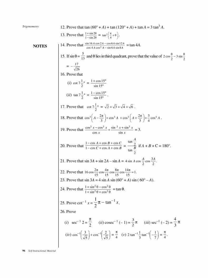
96 Self-Instructional Material
Trigonometry
NOTES
12. Prove that tan (60° + A) + tan (120° + A) + tan A = 3 tan3 A.
13. Prove that 1 sin 2θ
1 sin 2θ
+
− = 2 π
tan θ4
+
.
14. Prove that 2
sin 16 cos 2 cos 6 sin12
cos 4 cos sin 6 sin 8
A A A A
A A A A
−
− = tan 4A.
15. If sin θ = 13
5 and θ lies in third quadrant, prove that the value of
θ θ2 cos 3 sin
2 2−
= 17
26−
16. Prove that
(i) 1
cot 72
° = 1 cos 15
sin 15
+ °
°
(ii) 1
tan 72
° = 1 cos 15
sin 15
− °
°.
17. Prove that 1
cot 72
° = 2 3 4 6+ + + .
18. Prove that 3 32πcos cos
3A A
− +
3 32π 3cos cos
3 4A A
+ + =
.
19. Prove that 3 3 3 3cos cos sin sin
cos sin
x x x x
x x
− ++ = 3.
20. Prove that 1 cos cos cos
1 cos cos cos
A B C
C A B
− + +
− + + =
tan2
tan2
A
B if A + B + C = 180°.
21. Prove that sin 3A + sin 2A – sin A = 3
4 sin cos cos .2 2
A AA
22. Prove that 2π 4π 8π 14π
16 cos cos cos cos 1.15 15 15 15
=
23. Prove that sin 3A = 4 sin A sin (60° + A) sin ( 60° – A).
24. Prove that 2 2
2 2
1 sin θ cos θ
1 sin θ cos θ
+ −
+ + = tan θ.
25. Prove cot– 1x =
1
2
1π − −tan x .
26. Prove
(i) sec– 1 2 = π
2(ii) cosec– 1 (– 1) =
3
2π (iii) sec–1 (– 2) =
4
3π
(iv) cos cos− −FHGIKJ +
FHGIKJ
1 13
5
2
5 =
π
4 (v) 2
1
3
1
7
1 1tan tan− − −FHGIKJ =
π
4.
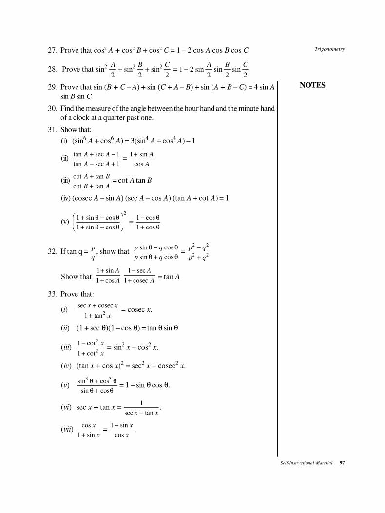
Trigonometry
NOTES
Self-Instructional Material 97
27. Prove that cos2 A + cos2 B + cos2 C = 1 – 2 cos A cos B cos C
28. Prove that sin sin sin2 2 2
2 2 2
A B C+ + = 1 2
2 2 2− sin sin sin
A B C
29. Prove that sin (B + C – A) + sin (C + A – B) + sin (A + B – C) = 4 sin A
sin B sin C
30. Find the measure of the angle between the hour hand and the minute hand
of a clock at a quarter past one.
31. Show that:
(i) (sin6A + cos6
A) = 3(sin4A + cos4
A) – 1
(ii)tan sec
tan sec
A A
A A
+ −
− +
1
1 =
1 + sin
cos
A
A
(iii)cot tan
cot tan
A B
B A
+
+ = cot A tan B
(iv) (cosec A – sin A) (sec A – cos A) (tan A + cot A) = 1
(v)1
1
2+ −
+ +
FHG
IKJ
sin cos
sin cos
θ θ
θ θ =
1
1
−
+
cos
cos
θ
θ
32. If tan q = p
q, show that
p q
p q
sin cos
sin cos
θ θ
θ θ
−
+ =
p q
p q
2 2
2 2
−
+
Show that 1 sin 1 sec
1 cos 1 cosec
A A
A A
+ +
+ + = tan A
33. Prove that:
(i)sec
tan
x x
x
+
+
cosec
1 2 = cosec x.
(ii) (1 + sec θ)(1 – cos θ) = tan θ sin θ
(iii)1
1
2
2
−
+
cot
cot
x
x = sin2
x – cos2x.
(iv) (tan x + cos x)2 = sec2x + cosec2
x.
(v)sin cos
sin cos
3 3θ θ
θ θ
+
+ = 1 – sin θ cos θ.
(vi) sec x + tan x = 1
sec tanx x−.
(vii)cos
sin
x
x1 + =
1 − sin
cos
x
x.
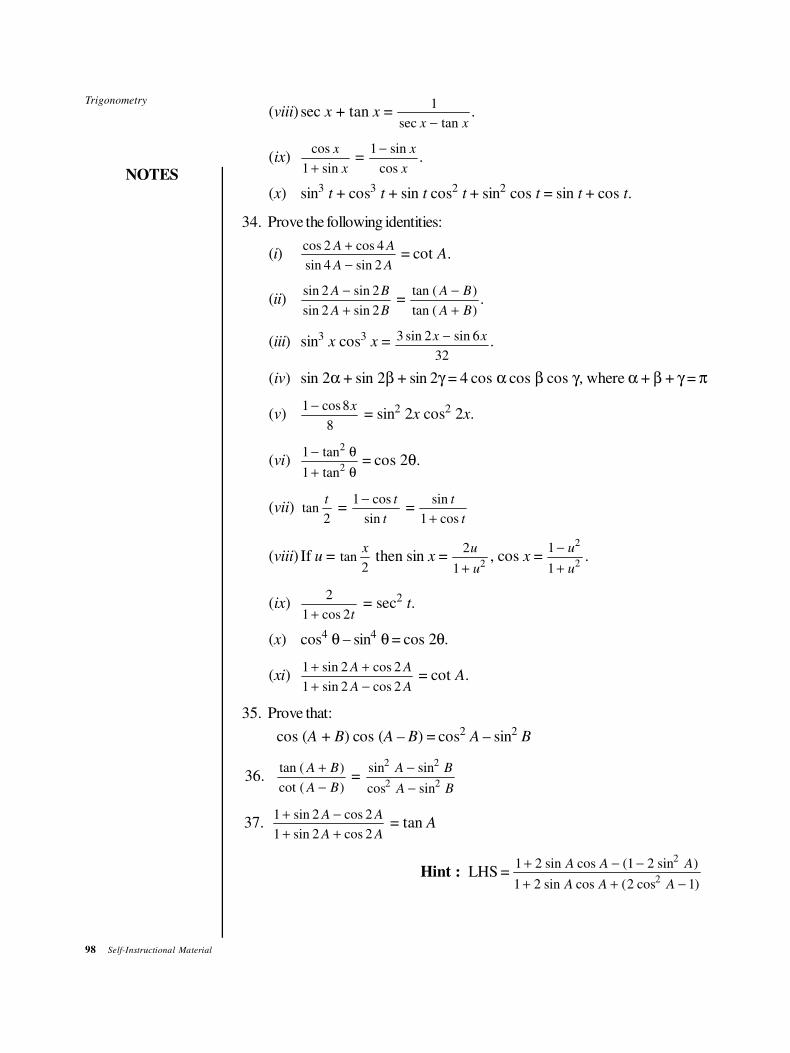
98 Self-Instructional Material
Trigonometry
NOTES
(viii) sec x + tan x = 1
sec tanx x−.
(ix)cos
sin
x
x1 + =
1 − sin
cos
x
x.
(x) sin3t + cos3
t + sin t cos2t + sin2 cos t = sin t + cos t.
34. Prove the following identities:
(i)cos cos
sin sin
2 4
4 2
A A
A A
+
− = cot A.
(ii)sin sin
sin sin
2 2
2 2
A B
A B
−
+ =
tan ( )
tan ( )
A B
A B
−
+.
(iii) sin3x cos3
x = 3 2 6
32
sin sinx x− .
(iv) sin 2α + sin 2β + sin 2γ = 4 cos α cos β cos γ, where α + β + γ = π
(v)1 8
8
− cos x = sin2 2x cos2 2x.
(vi)1
1
2
2
−
+
tan
tan
θ
θ = cos 2θ.
(vii) tant
2 =
1 − cos
sin
t
t =
sin
cos
t
t1 +
(viii) If u = tanx
2 then sin x =
2
1 2
u
u+, cos x =
1
1
2
2
−
+
u
u.
(ix)2
1 2+ cos t = sec2
t.
(x) cos4 θ – sin4 θ = cos 2θ.
(xi)1 2 2
1 2 2
+ +
+ −
sin cos
sin cos
A A
A A = cot A.
35. Prove that:
cos (A + B) cos (A – B) = cos2A – sin2
B
36.tan ( )
cot ( )
A B
A B
+
− =
sin sin
cos sin
2 2
2 2
A B
A B
−
−
37. 1 2 2
1 2 2
+ −
+ +
sin cos
sin cos
A A
A A = tan A
Hint : LHS = 1 2 1 2
1 2 2 1
2
2
+ − −
+ + −
sin cos ( sin )
sin cos ( cos )
A A A
A A A
Trigonometry
NOTES
Self-Instructional Material 99
38. If tan θ = b
a then a cos2 θ + b/2 sin 2θ = a.
a cos θ + b sin θ = a ba
a b
b
a b
2 2
2 2 2 2+
++
+
FHGG
IKJJ
cos sinθ θ
= a b2 2+ +(sin cos cos sin )α θ α θ
= a b2 2+ +sin ( )θ α , where tan α =
b
a.
39.sec
sec
8 1
4 1
A
A
−
− =
tan
tan
8
2
A
A(Note: sin 8A = 2 sin 4A cos 4A)
(Hint: LHS = 1 8
8
4
1 4
−
−
cos
cos
cos
cos
A
A
A
A =
2 4 4
8 2 2
2
2
sin cos
cos sin
A A
A A⋅
= sin sin cos
cos sin
4 2 4 4
8 2 22
A A A
A A
⋅ ⋅
⋅.)
40. If A + B + C = π/2 show
sin2A + sin2
B + sin2C = 1 – 2 sin A sin B sin C
41. If A + B = C then show
cos2A + cos2
B + cos2C = 1 + 2 cos A cos B cos C
42. Show sin2 30º sin 45º cos 45º = 1
8.
43. cos cos cos
cos cos cos
6 6 4 15 2 10
5 5 3 10
A A A
A A A
+ + +
+ + = 2 cos A.
[Hint: 2 cos A(cos 5A + 5 cos 3A + 10 cos A)]
= (cos 6A + cos 4A) + 5(cos 4A + cos 2A) + 10 (cos 2A + 1)
= cos 6A + 6 cos 4A + 15 cos 2A + 10
1.13 FURTHER READING
Khanna, V.K, S.K. Bhambri, C.B. Gupta and Vijay Gupta. Quantitative
Techniques. New Delhi: Vikas Publishing House.
Khanna, V.K, S.K. Bhambri and Quazi Zameeruddin. Business Mathematics.
New Delhi: Vikas Publishing House.

Differentiation
NOTES
Self-Instructional Material 101
UNIT 2 DIFFERENTIATION
Structure
2.0 Introduction2.1 Unit Objectives2.2 Limits and Continuity (Without Proof)
2.2.1 Functions and their Limits2.2.2 h-Method for Determining Limits
2.2.3 Expansion Method for Evaluating Limits2.2.4 Continuous Functions
2.3 Differentiation and Differential Coefficient2.4 Derivatives of Functions
2.4.1 Algebra of differentiable Functions
2.4.2 Differential Coefficients of Standard Functions2.4.3 Chain Rule of Differentiation
2.5 Derivatives: Tangent and Normal2.6 Differentiation of Implicit Functions and Parametric Forms
2.6.1 Parametric Differentiation
2.6.2 Logarithmic Differentiation
2.6.3 Successive Differentiation
2.7 Partial Differentiation2.8 Maxima and Minima of Functions
2.9 Summary2.10 Key Terms
2.11 Answers to ‘Check Your Progress’2.12 Questions and Exercises2.13 Further Reading
2.0 INTRODUCTION
In Mathematics, differentiation refers to the act of finding derivatives. Derivative is
defined as the instantaneous rate of change of a function. The derivative gives theslope of the tangent to the graph of the function at a point. Thus, it is a mathematicalformulation of the rate of change.
Differentiation expresses the rate of change of any quantity y with respect
to the change in another quantity x, with which it has a functional relationship.
2.1 UNIT OBJECTIVES
After going through this unit, you will be able to:
• Understand differentiation
• Understand how to check the continuity of functions
• Learn about differential coefficient
• Understand algebra of differentiable functions
• Analyse tangent and normal derivatives
102 Self-Instructional Material
Differentiation
NOTES
• Explain the differentiation of implicit functions and parametric forms
• Define partial differentiation
• Learn about maxima and minima of functions
2.2 LIMITS AND CONTINUITY (WITHOUT PROOF)
2.2.1 Functions and their Limits
In Mathematics, you usually deal with two kinds of quantities, namely constants
and variables. A quantity which is liable to vary is called a variable quantity or
simply a variable. Temperature, pressure, distance of a moving train from a
station are all variable quantities. On the other hand, a quantity that retains its value
through all mathematical operations is termed as a constant quantity or a con-
stant. Numbers like 4, 5, 2.5, π, etc., are all constants.
If x is a real variable (i.e., x takes up different values that are real numbers).
Then in quantities log x, sin x, x2, etc., log, sin, square are the functions.
Let us write y = x2.
Therefore, if x = 2, then y = 4, if x = 3, then y = 9, etc.
Thus, for each value of x, y gets a unique corresponding value and this value is
assigned each time by a certain rule (namely, square). This rule is what we call a
function.
So, in general, by a function of x, we mean a rule that gives us a unique value
corresponding to each value of x.
So, if y = sin x, then whenever we give a different value to x, we get a
corresponding unique value for y with the assistance of the function sine.
When we are dealing with any function, we simply write
y = f (x)
and say that y is a function of x although to be very correct we should say that y is
the value assigned by the function f corresponding to a value of x. And we call x as
the independent variable and y as dependent variable.
Functions play important role in Mathematics, Physics and Social Sciences.
A function which assigns a fixed value for every value of x is called a constant
function. For example, f (x) = 3 is a constant function, since for any value of x,
f (x) remains equal to 3.
The next important notion is that of the limit of a function. It is quite possible
that f (x) may not be defined for all values of x. As an illustration, consider
f (x) = x
x
2 25
5
−
−. This is a function of x, provided x takes all real values except 5. If
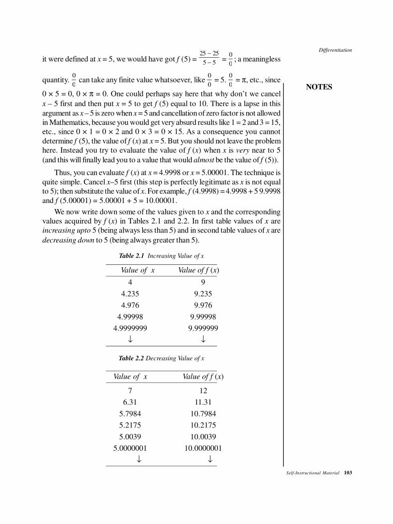
Differentiation
NOTES
Self-Instructional Material 103
it were defined at x = 5, we would have got f (5) = 25 25
5 5
−
− = 0
0; a meaningless
quantity. 0
0 can take any finite value whatsoever, like
0
0 = 5.
0
0 = π, etc., since
0 × 5 = 0, 0 × π = 0. One could perhaps say here that why don’t we cancel
x – 5 first and then put x = 5 to get f (5) equal to 10. There is a lapse in this
argument as x – 5 is zero when x = 5 and cancellation of zero factor is not allowed
in Mathematics, because you would get very absurd results like 1 = 2 and 3 = 15,
etc., since 0 × 1 = 0 × 2 and 0 × 3 = 0 × 15. As a consequence you cannot
determine f (5), the value of f (x) at x = 5. But you should not leave the problem
here. Instead you try to evaluate the value of f (x) when x is very near to 5
(and this will finally lead you to a value that would almost be the value of f (5)).
Thus, you can evaluate f (x) at x = 4.9998 or x = 5.00001. The technique is
quite simple. Cancel x–5 first (this step is perfectly legitimate as x is not equal
to 5); then substitute the value of x. For example, f (4.9998) = 4.9998 + 5 9.9998
and f (5.00001) = 5.00001 + 5 = 10.00001.
We now write down some of the values given to x and the corresponding
values acquired by f (x) in Tables 2.1 and 2.2. In first table values of x are
increasing upto 5 (being always less than 5) and in second table values of x are
decreasing down to 5 (being always greater than 5).
Table 2.1 Increasing Value of x
Value of x Value of f (x)
4 9
4.235 9.235
4.976 9.976
4.99998 9.99998
4.9999999 9.999999
↓ ↓
Table 2.2 Decreasing Value of x
Value of x Value of f (x)
7 12
6.31 11.31
5.7984 10.7984
5.2175 10.2175
5.0039 10.0039
5.0000001 10.0000001
↓ ↓
104 Self-Instructional Material
Differentiation
NOTES
The above is expressed mathematically as: x tends to 5 from the left
(in Table 2.1) and x tends to 5 from the right (in Table 2.2). In the first case we
write x → 5– and in the second case we write x → 5+.
Observe the pattern of change in the second column of each table. One could,
after slight concentration see that in the first situation f (x) → 10– while in the
second case f (x) → 10+. Thus, you are tempted to assert that f (x) approaches
10 (both from left and from right) as x approaches 5. This number 10, we call limit
of f (x) as x approaches 5.
This fact is denoted by, 5
Lim ( )x
f x→
= 10.
Consider now any small positive number, say, 0.01. When | x – 5 | < 0.01,
i.e., – 0.01 < x – 5 < 0.01 or 4.99 < x < 5.01, then – 0.01 < f (x) – 10 < 0.01
Or, | f (x) – 10 | < 0.01
(4.99 < x < 5.01 and x ≠ 5 ⇒ f (x) = x + 5
This yields in turn f (x) – 10 = x – 5
So, – 0.01 < f (x) – 10 < 0.01)
One can repeat the above experiment by starting with another small positive
number say 0.00002 and note that whenever | x – 5 | < 0.00002,
Then, | f (x) – 10 | < 0.00002.
The expected conclusion will be that, however a small positive number ε we
may start with, we shall always be able to find a δ > 0 such that whenever
| x – 5 | < δ then | f (x) – 10 | < ε. In the above illustration δ = ε will suffice.
Thus, you are led to the following definition of limit.
You say that Lim ( )x a
f x→
= l if corresponding to any ε > 0, we can find δ > 0,
such that | f (x) – l | < ε whenever | x – a | < δ.
Let us evaluate some limits using this definition. Later on we’ll give other con-
venient methods too.
Example 2.1: Evaluate Limx a
x→
.
Solution: Let ε > 0 be any number.
Take, δ = ε. Evidently δ > 0.
Now, | x – a | < δ ⇒ | f (x) – a | < ε
Since, f (x) = x.
Hence, Limx a
a→
.
Differentiation
NOTES
Self-Instructional Material 105
Example 2.2: Evaluate 2Lim
x ax
→.
Solution: Let ε > 0 be any number.
Take, δ = – 2 + 4 + ε . Clearly δ > 0
Now, | x + 2 | = | x – 2 + 4 | < | x – 2 | + 4 < δ + 4
So, | x – 2 | < δ ⇒ | x2 – 4 | = | x + 2 | |x – 2| < d2 + 4 δ = ε
Hence, 2
2Limx
x→
= 4.
Example 2.3: Determine 3
1Limx
.x→
Solution: Let ε > 0.
Put, δ = 9
1 3
ε
+ ε
Now, | x – 3 | < δ ⇒ | x – 3 | < 9
1 3
ε
+ ε...(1)
Also, | x – 3 | < δ ⇒ –δ < x – 3
⇒ x > 3 – δ = 3 – 9
1 3
ε
+ ε =
3
1 3+ ε
⇒1
x<
1 3
3
+ ε
...(2)
Equations (1) and (2) imply
1 1
3x− =
3
3
x
x
− <
9
1 3
ε
+ ε 1 3 1
3 3
+ ε⋅ = ε
Consequently, 3
1Limx x→
= 1
3.
Example 2.4: Find out the limit of 2 1
1
x
x
−
− as x → 1.
Solution: Let ε > 0 be any number.
Take δ = ε.
Now | x – 1 | < δ⇒ | x – 1 | <ε
⇒ | x + 1 – 2 | < ε
⇒2
12
1
x
x
−−
− < ε
⇒2
1
1Lim
1x
x
x→
−
− = 2.
106 Self-Instructional Material
Differentiation
NOTES
2.2.2 h-Method for Determining Limits
You put a + h in place of x and simplify such that h gets cancelled from denomina-
tor and numerator. Putting h = 0, you get limit of f (x) as x → a.
Example 2.5: Evalute
2
21
1Lim
1x
x
x→
−
−.
Solution: 3
21
1Lim
1x
x
x→
−
−=
3
20
(1 ) 1Lim
(1 ) 1h
h
h→
+ −
+ −
=
2 3
20
3 3Lim
2h
h h h
h h→
+ +
+
=
2
0
3 3Lim
2h
h h
h→
+ +
+
= 3
2.
2.2.3 Expansion Method for Evaluating Limits
This method is applicable to the functions which can be expanded in series. Fol-
lowing expansions are often utilized.
(1) (1 + x)n = 1 + nx + 2 3
( 1) ( 1)( 1)
2! 3!
n n x n n n x− − −+ + . . . provided | x | < 1
and n is any real number.
Note: If n is a positive integer, the expansion on RHS has finite number of
terms only.
(2) log (1 + x) = x – 2 3 4
. . .2 3 4
x x x+ − + ∞ provided | x | < 1.
(3) ex = 1 + x + 2 3
. . .2! 3!
x x+ + ∞
(4) sin x = x – 3 5
. . .3! 5!
x x+ ∞
(5) cos x = 1 – 2 4
. . .2! 4!
x x+ ∞
The method will be illustrated by means of the following examples.
Example 2.6: Show that 0
sinLimx
x
x→ = 1.
Solution:0
sinLimx
x
x→=
3 5
0
. . .3! 5!Lim
x
x xx
x→
− +
Differentiation
NOTES
Self-Instructional Material 107
=
2 4
0Lim 1 . . .
3! 5!x
x x
→
− +
= 1.
Note: The result of Example 2.6 shall be frequently used later on.
Example 2.7: Evaluate 0
Limx x
x
e e
x
−
→
−.
Solution: 0
Limx x
x
e e
x
−
→
−
=
2 3 2 3
0
1 . . . 1 . . .2! 3! 2! 3!
Limx
x x x xx x
x→
+ + + − − + −
=
3 5
0
2 .. .3! 5!
Limx
x xx
x→
+ +
=
2 4
0Lim 2 1 . . .
3! 5!x
x x
→
+ + +
= 2.
Notes:
1. 0
Lim ( )x
f x→
= l if and only if
Lim ( )x a
f x→ − = l = Lim ( )
x af x
→ + .
If one of the two equalities fails to hold, then we say that limit of f (x) as
x → a does not exist.
Consider 0
1Limx x→
. It can be easily seen that, if x → 0 –, then 1
x → – ∞ while,
if x → 0+, then 1
x → ∞ . So,
1
0Lim
xx→ does not exist.
2. If Limx a→
f(x) exists, then it must be unique.
Example 2.8: f(x) is defined as under
f (x) = 0 for x < 0
= 1
2 – x for x > 0.
Show that 2
( )Limx
f x→
does not exist.
Solution:0
Lim ( )x
f x→ −
= 0
(0 )Limh
f h→
− = 0.
Also,0
( )Limx
f x→ +
= 0
(0 )Limh
f h→ +
+ = 0
1Lim
2h
f h→
−
= 1
2
108 Self-Instructional Material
Differentiation
NOTES
Since, 0 0
Lim ( ) Lim ( )x x
f x f x→ − → +
≠ ,
0
Lim ( )x
f x→
does not exist.
Notes: 1. If Lim ( )x a
f x→
= l and Lim ( )x a
g x→
= m, then
(i) Lim[ ( ) ( )]x a
f x g x→
± = l ± m
(ii) Lim[ ( ) ( )]x a
f x g x→
= lm
(iii) ( )
Lim( )x a
f x
g x→ =
l
m provided m ≠ 0
(iv) ( )Lim[ ( )]g x
x a
f x→
= lm, provided lm is defined.
2. If f (x) < g (x) for all x, then Lim ( ) Lim ( )x a x a
f x g x→ →
≤ .
2.2.4 Continuous Functions
We have seen in Example 2.2 that 2
2Limx
x→
= 4, which is same as value of x2 at x = 2.
Whereas, in Example 2.4, 2
1
1Lim
1x
x
x→
−
− = 2, but the function itself is not defined as
x = 1.
Again consider, f (x) = 2 9
3
x
x
−
−, x ≠ 3
= 1, x = 3
In this case, 2
3
9Lim
3x
x
x→
−
−= 6, and f (3) = 1.
Thus, a function may possess a limit as x → a but it may or may not be defined
at x = a. Even if it is defined at x = a, its value may not be equal to its limit. This
prompts us to define the following type of functions.
A function f (x) is said to be continuous at x = a, if Lim ( )x a
f x→
= f (a).
In other words, f (x) is said to be continuous at x = a, if given ε > 0, there
exists δ > 0, such that | f (x) – f (a) | < ε, whenever | x – a | < δ.
Example 2.9: Check for continuity at x = 0, the function (x) = | x |.
Solution: By definition of absolute value, we can write.
f (x) = x for all x ≥ 0
= – x for all x < 0
We note that, f (0) = 0
Further,0
Lim ( )x
f x→ −
= 0
Lim (0 )h
f h→
− = 0
Lim ( )h
h→
− − = 0
Differentiation
NOTES
Self-Instructional Material 109
Also,0 0
Lim ( ) Lim (0 )x h
f x f h→ + →
+ = 0
Limh
h→
= 0.
Thus,0
Lim ( )h
f x→
= 0 = f (0)
Hence, f (x) is continuous at x = 0.
2.3 DIFFERENTIATION AND DIFFERENTIAL
COEFFICIENT
Let y be a function of x. We call x an independent variable and y dependent
variable.
Note: There is no sanctity about x being independent and y being dependent.This depends upon which variable we allow to take any value, and thencorresponding to that value, determine the value, of the other variable. Thus iny = x2, x is an independent variable and y a dependent, whereas the same function
can be re-written as x = y . Now y is an independent variable, and x is a depen-
dent variable. Such an ‘inversion’ is not always possible.
For example, in y = sin x + x3 + log x + x1/2, it is rather impossible to find x interms of y.
Differential coefficient of f (x) with respect to x
Let, y = f (x) ...(2.1)
and let x be changed to x + δx. If the corresponding change in y is δy, then
y + δy = f (x + δx) ...(2.2)
Equations (2.1) and (2.2) imply that
δy = f (x + δx) – f (x)
⇒δ
δ
y
x=
( δ ) ( )
δ
+ −f x x f x
x
δ 0
( δ ) ( )Lim
δ→
+ −
x
f x x f x
x
, if it exists, is called the differential coefficient of y
with respect to x and is written as dy
dx.
Thus,dy
dx= δ 0
δLim
δx
y
x→ =
δ 0
( δ ) ( )Lim
δx
f x x f x
x→
+ −.
Let f (x) be defined at x = a. The derivative of f (x) at x = a is defined as
0
( ) ( )Limh
f a h f a
h→
+ −, provided the limit exists, and then it is written as f′ (a) or
x a
dy
dx =
. We sometimes write the definition in the form f′ (a) =( ) ( )
Limx a
f x f a
x a→
−
−.
110 Self-Instructional Material
Differentiation
NOTES
Note: f′ (a) can also be evaluated by first finding out dy
dx and then putting in
it, x = a.
Notation: dy
dx is also denoted by y′ or y
1 or Dy or f′ (x) in case y = f (x).
Example 2.10: Find dy
dx and
3x
dy
dx =
for y = x3.
Solution: We have y = x3
Let δx be the change in x and let the corresponding change in y be δy.
Then, y + δy = (x + δx)3
⇒ δy = (x + δx)3 – y = (x + δx)3 – x3
= 3x2 (δx) + 3x (δx)2 + (δx)3
⇒δ
δ
y
x= 3x
2 + 3x (δx) + (δx)2
Consequently,dy
dx=
δ 0
δLim
δx
y
x→ = 3x
2
Also,3x
dy
dx =
= 3 . 32 = 27
Example 2.11: Show that for y = | x |, dy
dx does not exist at x = 0.
Solution: If dy
dx exists at x = 0, then
0
(0 ) (0)Lim h
f h f
h→
+ − exists.
So,0
(0 ) (0)Limh
f h f
h→ +
+ −=
0
(0 ) (0)Limh
f h f
h→ −
− −
−
Now, f (0 + h) = | h |,
So,0
(0 ) (0)Limh
f h f
h→ +
+ −=
0
0Limh
h
h→ +
− =
0Limh
h
h→ + = 1
Also,0
(0 ) (0)Limh
f h f
h→ −
− −
−=
0
0Limh
h
h→ −
− −
−
= 0
Limh
h
h→ − − = – 1
Hence,0
(0 ) (0)Limh
f h f
h→ +
+ −≠
0
(0 ) (0)Limh
f h f
h→ −
− −
−
Differentiation
NOTES
Self-Instructional Material 111
Consequently, 0
(0 ) (0)Limh
f h f
h→
+ − does not exist.
Notes: 1. A function f (x) is said to be derivable or differentiable at x = a if itsderivative exists at x = a.
2. A differentiable function is necessarily continuous.
Proof: Let f (x) be differentiable at x = a.
Then 0
( ) ( )Limh
f a h f a
h→
+ − exists, say, equal to l.
0
( ) ( )Limh
f a h f a
h→
+ − = 0
⇒ 0
Limh→
[ f (a + h) – f (a)] = 0
⇒ 0
Limh→
f (a + h) = f (a)
⇒ 0
Limh→
f (x) = f (a)
h can be positive or negative.
In other words f (x) is continuous at x = a.
3. Converse of the statement in Note 2 is not true in general.
Example 2.12: Show that f (x)= x2 sin
1
x, x ≠ 0 and x = 0
is differentiable at x = 0.
Solution: 0
( ) (0)Limh
f h f
h→
−
=
2
0
1sin 0
Limh
hh
h→
−
= 0
1Lim sinh
hh→
Now,1
sinh
< 1 and so 1
sinhh
< | h |
⇒0
1Lim sinh
hh→
≤ 0
Limh→
| h | = 0
Hence,0
( ) (0)Limh
f h f
h→
−= 0
i.e., f (x) is differentiable at x = 0
And f ′(0) = 0.
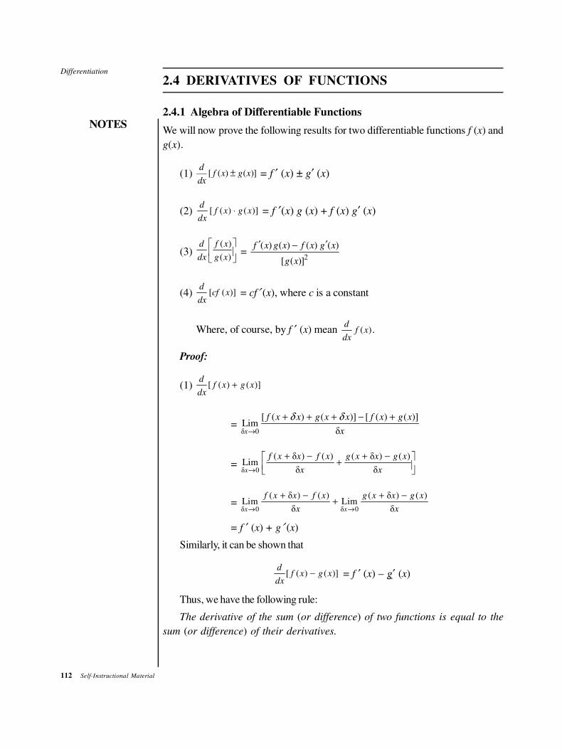
112 Self-Instructional Material
Differentiation
NOTES
2.4 DERIVATIVES OF FUNCTIONS
2.4.1 Algebra of Differentiable Functions
We will now prove the following results for two differentiable functions f (x) and
g(x).
(1) [ ( ) ( )]d
f x g xdx
± = f ′ (x) ± g′ (x)
(2) [ ( ) ( )]⋅d
f x g xdx
= f ′(x) g (x) + f (x) g′ (x)
(3) ( )
( )
d f x
dx g x
= 2
( ) ( ) ( ) ( )
[ ( )]
f x g x f x g x
g x
′ ′−
(4) [ ( )]d
cf xdx
= cf′ (x), where c is a constant
Where, of course, by f ′ (x) mean ( )d
f xdx
.
Proof:
(1) [ ( ) ( )]+d
f x g xdx
= δ 0
[ ( ) ( )] [ ( ) ( )]Lim
δx
f x x g x x f x g x
x
δ δ
→
+ + + − +
= δ 0
( δ ) ( ) ( δ ) ( )Lim
δ δx
f x x f x g x x g x
x x→
+ − + − +
= δ 0 δ 0
( δ ) ( ) ( δ ) ( )Lim Lim
δ δx x
f x x f x g x x g x
x x→ →
+ − + −+
= f ′ (x) + g′ (x)
Similarly, it can be shown that
[ ( ) ( )]−d
f x g xdx
= f ′ (x) – g′ (x)
Thus, we have the following rule:
The derivative of the sum (or difference) of two functions is equal to the
sum (or difference) of their derivatives.
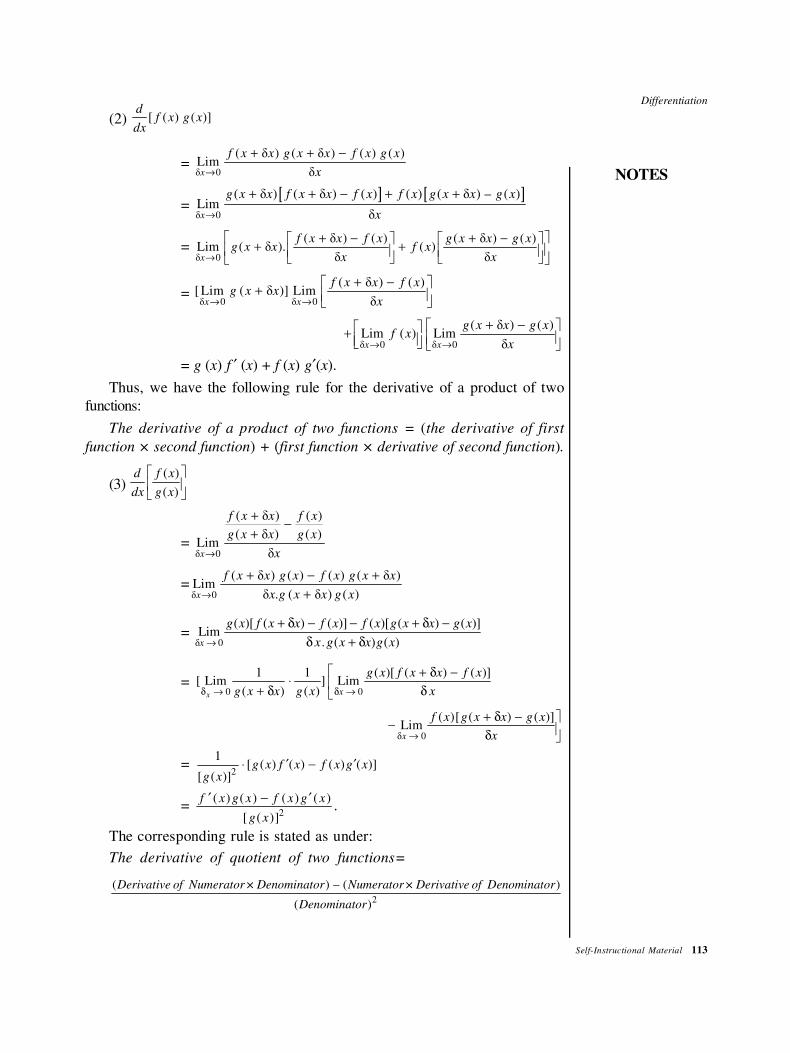
Differentiation
NOTES
Self-Instructional Material 113
(2) [ ( ) ( )]d
f x g xdx
= δ 0
( δ ) ( δ ) ( ) ( )Lim
δx
f x x g x x f x g x
x→
+ + −
= [ ] [ ]
δ 0
( δ ) ( δ ) ( ) ( ) ( δ ) – ( )Lim
δx
g x x f x x f x f x g x x g x
x→
+ + − + +
= δ 0
( δ ) ( ) ( δ ) ( )Lim ( δ ). ( )
δ δx
f x x f x g x x g xg x x f x
x x→
+ − + − + +
= δ 0 δ 0
( δ ) ( )[ Lim ( δ )] Lim
δx x
f x x f xg x x
x→ →
+ − +
δ 0 δ 0
( δ ) ( )Lim ( ) Lim
δx x
g x x g xf x
x→ →
+ − +
= g (x) f ′ (x) + f (x) g′(x).
Thus, we have the following rule for the derivative of a product of two
functions:
The derivative of a product of two functions = (the derivative of first
function × second function) + (first function × derivative of second function).
(3)( )
( )
d f x
dx g x
= δ 0
( δ ) ( )
( δ ) ( )Lim
δx
f x x f x
g x x g x
x→
+−
+
=δ 0
( δ ) ( ) ( ) ( δ )Lim
δ . ( δ ) ( )x
f x x g x f x g x x
x g x x g x→
+ − +
+
= δ 0
( )[ ( ) ( )] ( )[ ( ) ( )]Lim
. ( ) ( )x
g x f x x f x f x g x x g x
x g x x g x→
+ δ − − + δ −
δ + δ
= 0 0
1 1 ( )[ ( ) ( )][ Lim ] Lim
( ) ( )x x
g x f x x f x
g x x g x xδ → δ →
+ δ −⋅
+ δ δ
δ 0
( )[ ( ) ( )]Limx
f x g x x g x
x→
+ δ − − δ
= 2
1[ ( ) ( ) ( ) ( )]
[ ( )]g x f x f x g x
g x
⋅ ′ − ′
= f x g x f x g x
g x
′ − ′( ) ( ) ( ) ( )
[ ( )]2.
The corresponding rule is stated as under:
The derivative of quotient of two functions=
2
( ) – ( )
( )
Derivative of Numerator × Denominator Numerator × Derivative of Denominator
Denominator
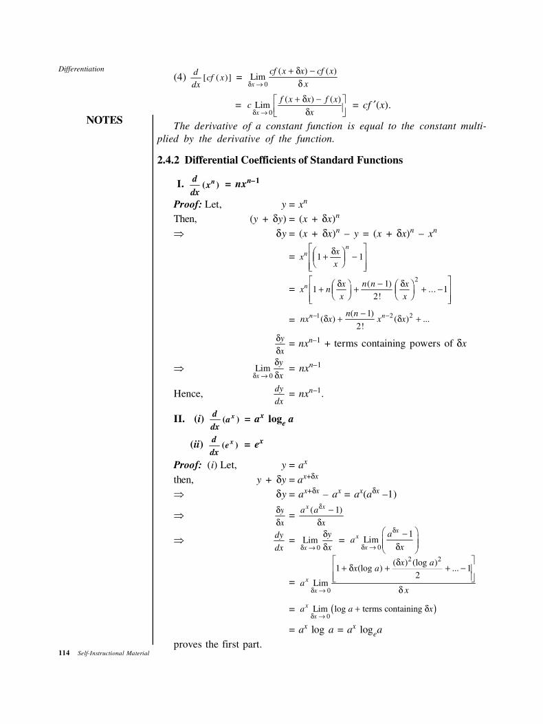
114 Self-Instructional Material
Differentiation
NOTES
(4) d
dxcf x[ ( )] =
0
( ) ( )Limx
cf x x cf x
xδ →
+ δ −
δ
= 0
( ) ( )Limx
f x x f xc
xδ →
+ δ − δ
= cf ′(x).
The derivative of a constant function is equal to the constant multi-
plied by the derivative of the function.
2.4.2 Differential Coefficients of Standard Functions
I. ( )ndx
dx = nxn–1
Proof: Let, y = xn
Then, (y + δy) = (x + δx)n
⇒ δy = (x + δx)n – y = (x + δx)n – xn
= xx
x
n
n
1 1+FHGIKJ −
LNMM
OQPP
δ
= x nx
x
n n x
x
n 11
21
2
+FHGIKJ +
− FHGIKJ + −
LNMM
OQPP
δ δ( )
!...
= 1 2 2( 1)( ) ( ) ...
2!
− −−δ + δ +n nn n
nx x x x
δ
δ
y
x= nx
n–1 + terms containing powers of δx
⇒0
Limx
y
xδ →
δ
δ= nx
n–1
Hence,dy
dx= nx
n–1.
II. (i) ( )xda
dx = ax loge a
(ii) ( )xd
edx
= ex
Proof: (i) Let, y = ax
then, y + δy = ax+δx
⇒ δy = ax+δx – a
x = ax(aδx –1)
⇒δ
δ
y
x=
a a
x
x x( )δ
δ
− 1
⇒dy
dx=
0Limx
y
xδ →
δ
δ =
0
1Lim
xx
x
aa
x
δ
δ →
− δ
=
2 2
0
( ) (log )1 (log ) ... 1
2Lim
x
x
x ax a
axδ →
δ+ δ + + −
δ
= ( )0
Lim log terms containing x
x
a a xδ →
+ δ
= ax log a = ax logea
proves the first part.
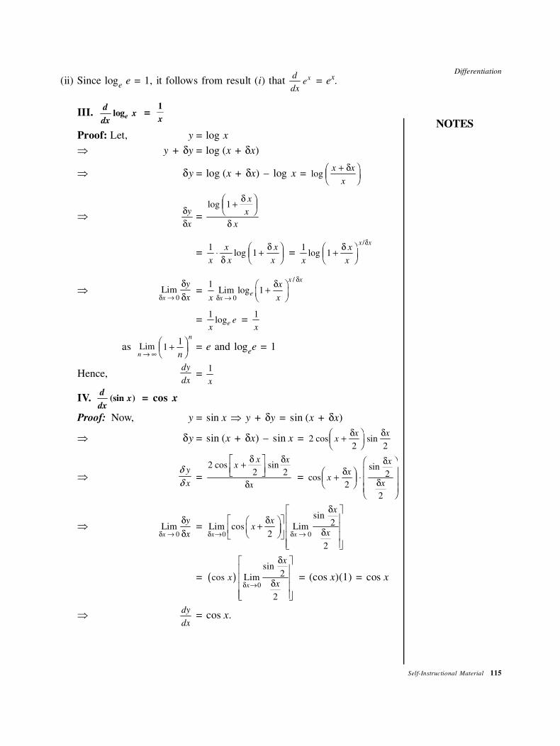
Differentiation
NOTES
Self-Instructional Material 115
(ii) Since loge e = 1, it follows from result (i) that
d
dxe
x = ex.
III. loge
dx
dx =
1
x
Proof: Let, y = log x
⇒ y + δy = log (x + δx)
⇒ δy = log (x + δx) – log x = logx x
x
+FHG
IKJ
δ
⇒δ
δ
y
x=
log 1 +FHG
IKJ
δ
δ
x
x
x
= 1
1x
x
x
x
x⋅ +
FHG
IKJδ
δlog =
11
x
x
x
x x
log
/
+FHG
IKJ
δδ
⇒0
Limx
y
xδ →
δ
δ=
/
0
1Lim log 1
x x
ex
x
x x
δ
δ →
δ +
= 1
xeelog =
1
x
as Limn → ∞
n
n+FHGIKJ1
1= e and log
ee = 1
Hence,dy
dx=
1
x
IV. (sin )d
xdx
= cos x
Proof: Now, y = sin x ⇒ y + δy = sin (x + δx)
⇒ δy = sin (x + δx) – sin x = 22 2
cos sinxx x
+FHG
IKJ
δ δ
⇒y
x
δ
δ=
22 2
cos sinxx x
x
+LNM
OQP
δ δ
δ = cos
sin
xx
x
x+FHG
IKJ ⋅F
HGGG
I
KJJJ
δδ
δ2
2
2
⇒0
Limx
y
xδ →
δ
δ=
0 0
sin2Lim cos Lim
2
2
x x
x
xx
xδ → δ →
δ δ
+ δ
= ( )0
sin2cos Lim
2
x
x
xxδ →
δ δ
= (cos x)(1) = cos x
⇒dy
dx= cos x.
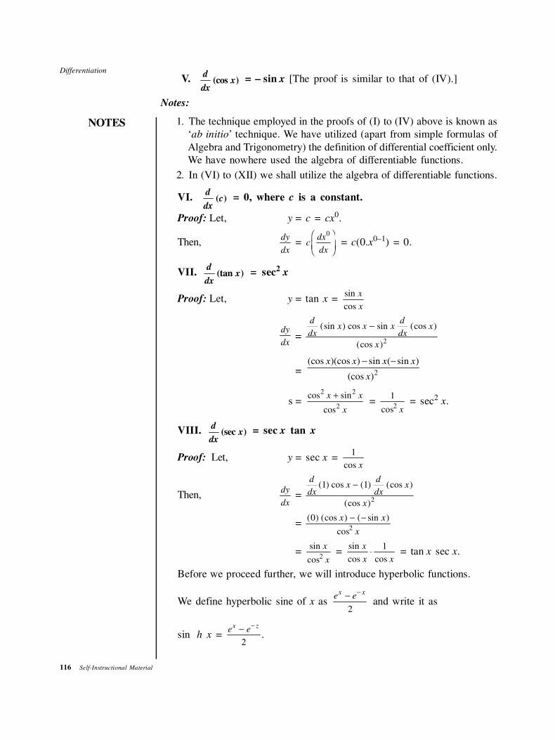
116 Self-Instructional Material
Differentiation
NOTES
V. (cos )d
xdx
= – sin x [The proof is similar to that of (IV).]
Notes:
1. The technique employed in the proofs of (I) to (IV) above is known as
‘ab initio’ technique. We have utilized (apart from simple formulas of
Algebra and Trigonometry) the definition of differential coefficient only.
We have nowhere used the algebra of differentiable functions.
2. In (VI) to (XII) we shall utilize the algebra of differentiable functions.
VI. ( )d
cdx
= 0, where c is a constant.
Proof: Let, y = c = cx0.
Then,dy
dx= c
dx
dx
0FHGIKJ = c(0.x0–1) = 0.
VII. (tan )d
xdx
= sec2 x
Proof: Let, y = tan x = sin
cos
x
x
dy
dx=
d
dxx x x
d
dxx
x
(sin ) cos sin (cos )
(cos )
−
2
= 2
(cos )(cos ) sin ( sin )
(cos )
x x x x
x
− −
s = 2 2
2
cos sin
cos
+x x
x
= 12cos x
= sec2x.
VIII. (sec )d
xdx
= sec x tan x
Proof: Let, y = sec x = 1
cos x
Then,dy
dx=
d
dxx
d
dxx
x
( ) cos ( ) (cos )
(cos )
1 1
2
−
= ( ) (cos ) ( sin )
cos
02
x x
x
− −
= sin
cos
x
x2
= sin
cos cos
x
x x⋅
1 = tan x sec x.
Before we proceed further, we will introduce hyperbolic functions.
We define hyperbolic sine of x as 2
−−x xe e
and write it as
sin h x = e e
x z− −
2.
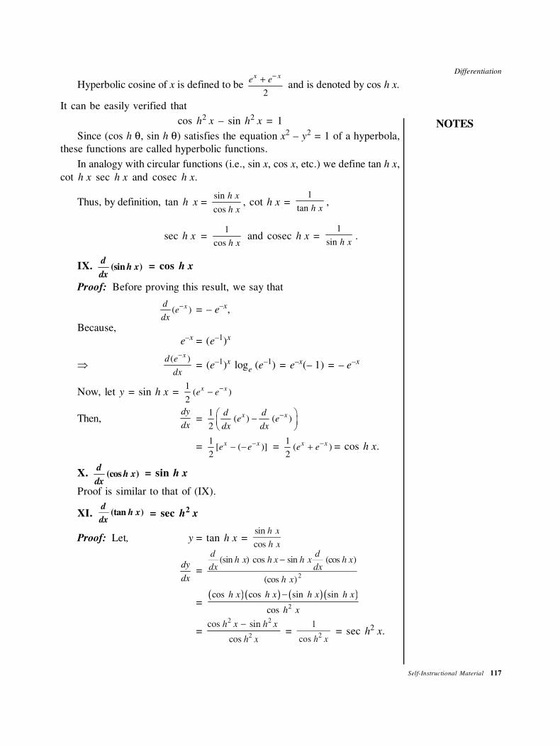
Differentiation
NOTES
Self-Instructional Material 117
Hyperbolic cosine of x is defined to be 2
−+x xe e
and is denoted by cos h x.
It can be easily verified that
cos h2
x – sin h2
x = 1
Since (cos h θ, sin h θ) satisfies the equation x2 – y2 = 1 of a hyperbola,
these functions are called hyperbolic functions.
In analogy with circular functions (i.e., sin x, cos x, etc.) we define tan h x,
cot h x sec h x and cosec h x.
Thus, by definition, tan h x = xh
xh
cos
sin, cot h x =
xhtan
1,
sec h x = xhcos
1 and cosec h x =
xhsin
1.
IX. (sin )d
h xdx
= cos h x
Proof: Before proving this result, we say that
( )−xde
dx= – e
–x,
Because,
e–x = (e–1)x
⇒( )
−xd e
dx= (e–1)x log
e(e–1) = e
–x(– 1) = – e–x
Now, let y = sin h x = 1
( )2
−−x xe e
Then,dy
dx=
1( ) ( )
2
− −
x xd de e
dx dx
= 1
[ ( )]2
−− −x xe e =
1( )
2
−+x xe e = cos h x.
X. (cos )d
h xdx
= sin h x
Proof is similar to that of (IX).
XI. (tan )d
h xdx
= sec h2 x
Proof: Let, y = tan h x = sin h
cos h
x
x
dy
dx=
d
dxx x x
d
dxx
x
(sin h ) cos h (cos h )
(cos h )
−
2
sin h
= ( )( ) ( ) ( )
2
cos cos sin sin
cos
h x h x h x h x
h x
−
= cos h sin h
cos h
2 2
2
x x
x
− =
1
cos h2
x = sec h
2x.
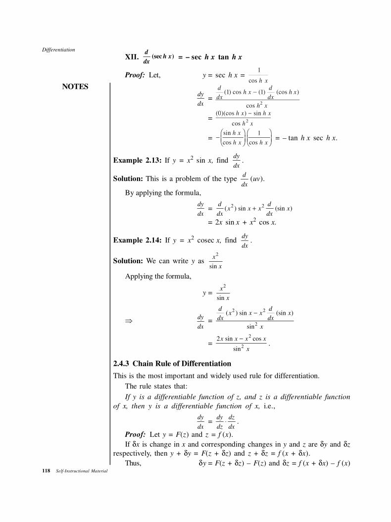
118 Self-Instructional Material
Differentiation
NOTES
XII. (sec )d
h xdx
= – sec h x tan h x
Proof: Let, y = sec h x = 1
cos h x
dy
dx=
d
dxx
d
dxx
x
( ) cos h ( ) (cos h )
cos h
1 1
2
−
= ( )(cos h ) sin h
cos h
02
x x
x
−
= −FHGIKJFHGIKJ
sin h
cos h cos h
x
x x
1 = – tan h x sec h x.
Example 2.13: If y = x2 sin x, find
dy
dx.
Solution: This is a problem of the type d
dx(uv).
By applying the formula,
dy
dx=
d
dxx x x
d
dxx( ) sin (sin )2 2+
= 2x sin x + x2 cos x.
Example 2.14: If y = x2 cosec x, find
dy
dx.
Solution: We can write y as x
x
2
sin
Applying the formula,
y = x
x
2
sin
⇒ dy
dx=
d
dxx x x
d
dxx
x
( ) sin (sin )
sin
2 2
2
−
= 2
2
2
x x x x
x
sin cos
sin
−.
2.4.3 Chain Rule of Differentiation
This is the most important and widely used rule for differentiation.
The rule states that:
If y is a differentiable function of z, and z is a differentiable function
of x, then y is a differentiable function of x, i.e.,
dy
dx=
dy
dz
dz
dx⋅ .
Proof: Let y = F(z) and z = f (x).
If δx is change in x and corresponding changes in y and z are δy and δz
respectively, then y + δy = F(z + δz) and z + δz = f (x + δx).
Thus, δy = F(z + δz) – F(z) and δz = f (x + δx) – f (x)
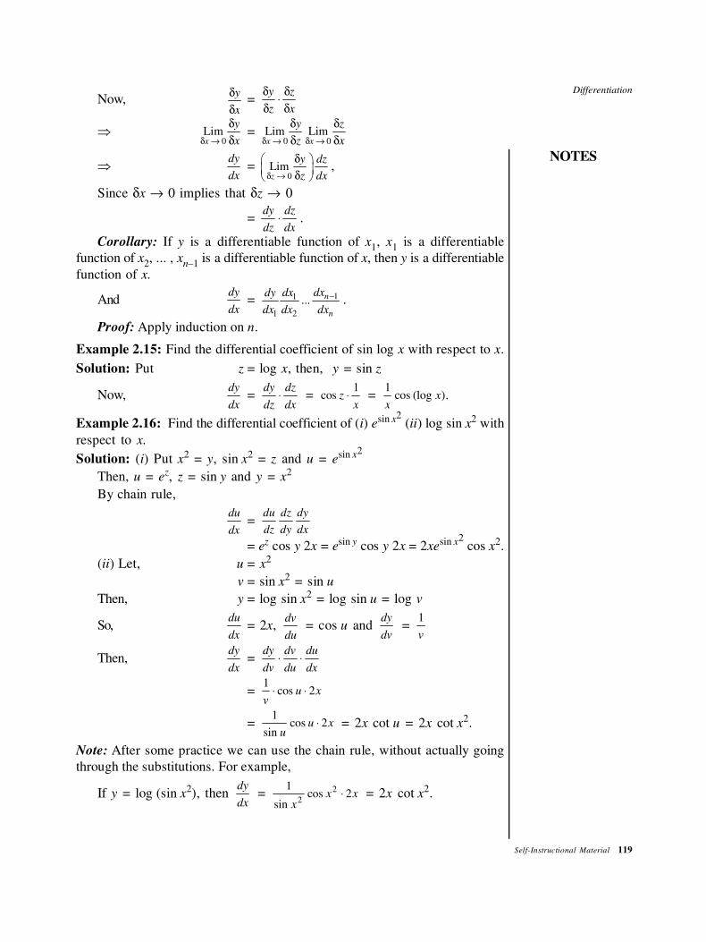
Differentiation
NOTES
Self-Instructional Material 119
Now,δ
δ
y
x=
δ
δ
δ
δ
y
z
z
x⋅
⇒0
Limx
y
xδ →
δ
δ=
0 0Lim Limx x
y z
z xδ → δ →
δ δ
δ δ
⇒dy
dx=
0Limz
y dz
z dxδ →
δ
δ ,
Since δx → 0 implies that δz → 0
= dy
dz
dz
dx⋅ .
Corollary: If y is a differentiable function of x1, x1 is a differentiable
function of x2, ... , xn–1 is a differentiable function of x, then y is a differentiable
function of x.
Anddy
dx= 11
1 2
... n
n
dxdxdy
dx dx dx
− .
Proof: Apply induction on n.
Example 2.15: Find the differential coefficient of sin log x with respect to x.
Solution: Put z = log x, then, y = sin z
Now,dy
dx=
dy
dz
dz
dx⋅ = cos z
x⋅
1 =
1
xxcos (log ).
Example 2.16: Find the differential coefficient of (i) esin x2 (ii) log sin x
2 with
respect to x.
Solution: (i) Put x2 = y, sin x
2 = z and u = esin x
2
Then, u = ez, z = sin y and y = x
2
By chain rule,
du
dx=
du
dz
dz
dy
dy
dx
= ez cos y 2x = esin y cos y 2x = 2xesin x
2 cos x
2.
(ii) Let, u = x2
v = sin x2 = sin u
Then, y = log sin x2 = log sin u = log v
So,du
dx= 2x,
dv
du = cos u and
dy
dv =
1
v
Then,dy
dx=
dy
dv
dv
du
du
dx⋅ ⋅
= 1
2v
u x⋅ ⋅cos
= 1
2sin
cosu
u x⋅ = 2x cot u = 2x cot x2.
Note: After some practice we can use the chain rule, without actually going
through the substitutions. For example,
If y = log (sin x2), then
dy
dx =
12
2
2
sincos
x
x x⋅ = 2x cot x2.
120 Self-Instructional Material
Differentiation
NOTES
Note that we have first differentiated log function according to the formula
d
dtt(log ) =
1
t. Since, here we have log (sin x
2), so the first term on differentiation
is 1
2sin x
.
Now, consider sin x2 and differentiate it according to the formula
d
duu(sin )
= cos u. Thus, the second term is cos x2.
Finally, we differentiated x2 with respect to x, so, the third term is 2x.
Then, we multiplied all these three terms to get the answer 2x cot x2. We
will illustrate this quick method by few more examples.
Example 2.17: Find dy
dx, when y =
3(2 3)xe
+ .
Solution: Since,d e
dt
t( )= et and
du
du
3
= 3u2
Andd v
dv
( )2= 2
We get,dy
dx=
2(2 3) 23(2 3) (2.1 0)x
e x+ ⋅ + ⋅ + = 6 2 3 2 2 3
2
( ) ( )x e
x+ +
Example 2.18: Differentiate y = log [sin (3x2 + 5)] with respect to x.
Solution:dy
dx=
1
3 53 5 6
2
2
sin ( )cos ( )
x
x x
++ = 6x cot (3x
2 + 5).
Example 2.19: Differentiate y = tan2 ( 3x + ).
Solution:dy
dx= 2 3 3
1
2
2tan ( ) sec ( )x x
x
+ ⋅ + ⋅ = tan ( ) sec ( )x x
x
+ +3 32
.
CHECK YOUR PROGRESS
1. Find out the limit of 2
1
1
x
x
−
− as x → 1.
2. Find dy
dx and
3x
dy
dx =
for y = x3.
3. When is a function f (x) differentiable at x = a?
4. Differentiate following two functions with respect to x :
3x2 – 6x + 1 and (2x
2 + 5x – 7)5/2
5. How will you calculate the derivative of a product of two functions?
6. What do you understand by the chain rule of differentiation?
Differentiation
NOTES
Self-Instructional Material 121
2.5 DERIVATIVES: TANGENT AND NORMAL
Figure 2.1 shows the tangent and normal of function y= f(x).
Let P (x′, y′) be any point on the curve y = f(x). Equation of any line through
(x′, y′) is
y – y′ = m(x – x′)
In case this line is tangent at P, its slope must be equal to the value of dy
dx at
(x′, y′).
Let us denote the value of dy
dx at (x′, y′) by
dy
dx
′
Thus, m =dy
dx
′
Hence, the equation of tangent at (x′, y′) of y = f(x) is given by
y – y′ =dy
dx
′
(x – x′)
Sometimes this formula is written as
Y – y′ =dy
dx
(X – x),
Where, X and Y are current coordinates and (x, y) is the given point (i.e., the
point of contact).
A normal at a point P of a plane curve y = f(x) is a line through P in the plane
of curve, perpendicular to the tangent there at P.
So, if PT is tangent to a curve y = f(x) at a point P, and if PN is perpendicular
to PT, then PN is normal to the curve at P.
The equation of normal at P (x′, y′) is, therefore,
y – y′ = 1
dy
dx
′
(x – x′)
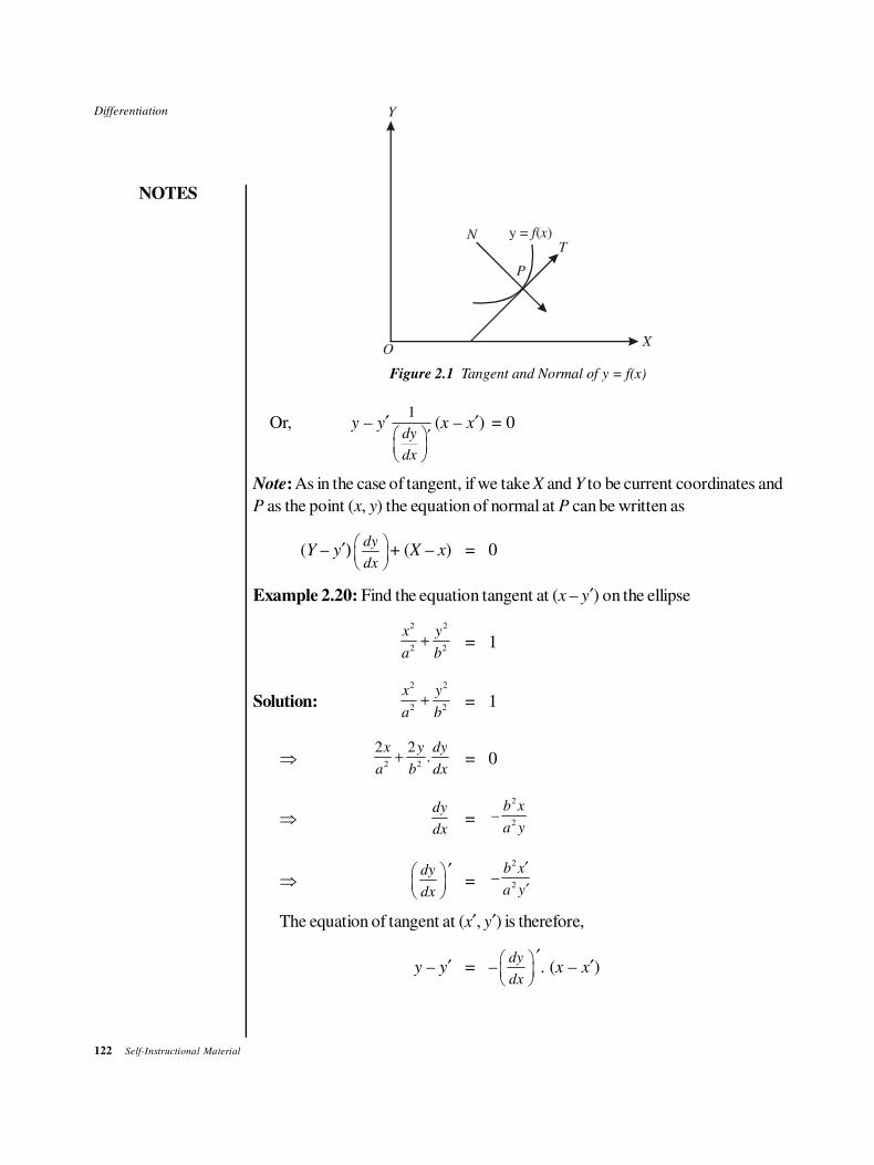
122 Self-Instructional Material
Differentiation
NOTES
O
Y
N
P
X
y = ( )f x
T
Figure 2.1 Tangent and Normal of y = f(x)
Or, y – y′1
dy
dx
′
(x – x′) = 0
Note: As in the case of tangent, if we take X and Y to be current coordinates and
P as the point (x, y) the equation of normal at P can be written as
(Y – y′)dy
dx
+ (X – x) = 0
Example 2.20: Find the equation tangent at (x – y′) on the ellipse
2 2
2 2
x y
a b+ = 1
Solution:2 2
2 2
x y
a b+ = 1
⇒ 2 2
2 2.
x y dy
a b dx+ = 0
⇒dy
dx=
2
2–
b x
a y
⇒dy
dx
′=
2
2–
b x
a y
′
′
The equation of tangent at (x′, y′) is therefore,
y – y′ = –dy
dx
′. (x – x′)
Differentiation
NOTES
Self-Instructional Material 123
Or, y – y′ =2
2–
b x
a y
′
′
(x – x′)
⇒ a2 yy′ – a2 y′2 = –b2 xx′ + b2x′2
⇒ b2 xx′ – a2 yy′ = b2 x′2 + a2y′2
⇒ 2 2
xx yy
a b
′ ′+ = 2 2
x y
a b
2 2′ ′+
= 1, since (x′ – y′) lies on the ellipse.
Example 2.21: Find the equation of normal at a point (x′ – y′) on the curve
y = a log sin x.
Solution: Here,dy
dx= a
1
sin xcos x = a cot x
⇒dy
dx
′= a cot x′
So, the normal has equation
(y – y′) a cos x′ + (x – x′) = 0
i.e.,
a(y – y′) a cos x′ + (x – x′) sin x2 = 0
Example 2.22: Find the equation of tangent at a point (2, 2) on the curve
y2= 2x.
Solution: Differentiating y2 = 2x with respect to x, we get
2dy
ydx
= 2
⇒dy
dx=
1
y
So, dy
dxat the point (2, 2) is equal to
1
2.
i.e.,dy
dx
′=
1
2
Hence, the equation of tangent to y2 = 2x at (2, 2) is
y – y′ =dy
dx
′ (x – x′)
i.e., y – 2 =1
2(x – 2)
Or, 2y – 4 = (x – 2)
⇒ x – 2y + 2 = 0
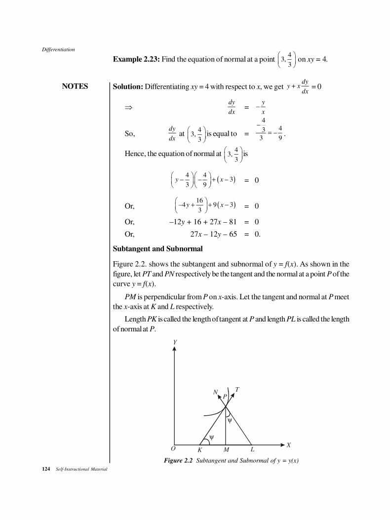
124 Self-Instructional Material
Differentiation
NOTES
Example 2.23: Find the equation of normal at a point 4
3,3
on xy = 4.
Solution: Differentiating xy = 4 with respect to x, we get dy
y + xdx
= 0
⇒dy
dx=
y–
x
So,dy
dx at
43,
3
is equal to =
4–
43 –3 9
= .
Hence, the equation of normal at 4
3,3
is
( )4 4
– – – 33 9
y x
+
= 0
Or, ( )16
–4 9 33
y x
+ + −
= 0
Or, –12y + 16 + 27x – 81 = 0
Or, 27x – 12y – 65 = 0.
Subtangent and Subnormal
Figure 2.2. shows the subtangent and subnormal of y = f(x). As shown in the
figure, let PT and PN respectively be the tangent and the normal at a point P of the
curve y = f(x).
PM is perpendicular from P on x-axis. Let the tangent and normal at P meet
the x-axis at K and L respectively.
Length PK is called the length of tangent at P and length PL is called the length
of normal at P.
O
Y
NP
X
T
K M L
ψ
ψ
Figure 2.2 Subtangent and Subnormal of y = y(x)
Differentiation
NOTES
Self-Instructional Material 125
Further, KM, i.e., the projection of KP on x-axis is called subtangent at P and
LM, the projection of PL on x-axis is called the subnormal at P.
Suppose that (x′, y′) are the coordinates of P, then if ψ is the angle TKL,
dy
dx
= tan ψ
– – –2 2 2
M PL M PLπ π π
∠ = ∠ = ψ = ψ
So, subtangent at P = KM = PM KM
PM = y′ cot ψ
= y′ 1
dy
dx
′
=y
dy
dx
′
′
Whereas, subnormal at P = LM = PM. LM
PM= y2 tan ψ
= y′ dy
dx
′
The length of tangent at P = PK will be
= 2 2PM KM+
= ( )
2
2
dy
dx
yy
′′ +
′
=
2
1y dy
dy dx
dx
′ + ′
=
2
1y dy
dy dx
dx
′ ′+ ′
Also, the length of normal at P = PL will be
= 2 2PM LM+
=
2
2 dyy y
dx
′ ′ + ′
= y′ 2
1dy
dx
′ +
126 Self-Instructional Material
Differentiation
NOTES
Example 2.24: Prove that for the parabola y2 = 4ax, subtangent at any point is
twice its abscissa and subnormal is constant.
Solution: Let (x′, y′) be any point on y′2 = 4ax.
So, y′2 = 4ax′ ...(1)
Differentiating, we get
2y dy
dx= 4a ⇒
2dy a
dx y=
⇒dy
dx
′
=2a
y′
Hence, the subtangent at (x′, y′) is
y y
dy a
dx y
′ ′=
′ 2
′
=2
y
a
′
=4
2
ax
a
′, by Equation (1)
= 2x′
= twice the abscissae of the point P.
Also, the subnormal at P is equal to y′ dy
dx
′
= y′.2a
y′ = 2a, a constant.
Example 2.25: Find the lengths of tangent and normal at any point (x′, y′) of the
curve y = 2
a
( )/ – /x a x ae e+ .
Solution: Here, y =2
a
( )/ – /x a x ae e+
= a cosh x
a
⇒dy
dx=
1sin
xa h
a a
= sinh x
a
This gives thatdy
dx
′
= sinh x
a
′
Differentiation
NOTES
Self-Instructional Material 127
Then, the length of the tangent at (x′, y′) is
2
1y dy
dy dx
dx
′ ′+ ′
=
2cos 1 sin
sin
x xa h h
a a
xh
a
′ ′+
′
As (x′, y′) lies on the given curve.
=
cos
cos
sin
xa h
xah
x ah
a
′′
′
= a cosx
ha
′cot
xh
a
′
Also, the length of normal at (x′, y′) is
2
1dy
ydx
′′ +
= cos 1 sin 2x xa h h
a a
′ ′ +
= 2cos
xa h
a
′
2.6 DIFFERENTIATION OF IMPLICIT FUNCTIONS
AND PARAMETRIC FORMS
2.6.1 Parametric Differentiation
When x and y are separately given as functions of a single variable t (called
a parameter), then you should first evaluate dx
dt and
dy
dt and then use chain
formula dy
dt =
dy
dx
dx
dt, to obtain
dy
dx=
dy
dt
dx
dt
The equations x = F (t) and y = G(t) are called parametric equations.
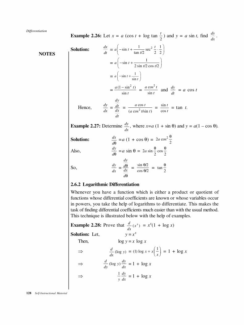
128 Self-Instructional Material
Differentiation
NOTES
Example 2.26: Let x = a (cos t + log tant
2) and y = a sin t, find
dy
dx.
Solution:dx
dt= 21 1
sin sectan /2 2 2
− + ⋅
ta t
t
=1
sin2 sin /2 cos /2
− +
a tt t
=1
sinsin
− +
a tt
=a t
t
( sin )
sin
1 2− =
a t
t
cos
sin
2
and dy
dt = a cos t
Hence,dy
dx=
dy
dt
dx
dt
= 2
cos
( cos /sin )
a t
a t t =
sin
cos
t
t = tan t.
Example 2.27: Determine dy
dx, where x=a (1 + sin θ) and y = a(1 – cos θ).
Solution:dx
dθ=a (1 + cos θ) = 2
2
2a cos
θ
Also,dy
dθ=a sin θ = 2
2 2a sin cos
θ θ
So,dy
dx=
dy
d
dx
d
θ
θ
= sin /2
cos /2
θ
θ = tan
θ
2
2.6.2 Logarithmic Differentiation
Whenever you have a function which is either a product or quotient of
functions whose differential coefficients are known or whose variables occur
in powers, you take the help of logarithms to differentiate. This makes the
task of finding differential coefficients much easier than with the usual method.
This technique is illustrated below with the help of examples.
Example 2.28: Prove that d
dxx
x( ) = x
x(1 + log x)
Solution: Let, y = xx
Then, log y = x log x
⇒ d
dxy(log ) = ( ) log1
1x x
x+FHGIKJ = 1 + log x
⇒d
dyy
dy
dx(log ) = 1 + log x
⇒1
y
dy
dx= 1 + log x
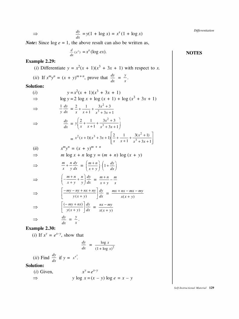
Differentiation
NOTES
Self-Instructional Material 129
⇒ dy
dx= y(1 + log x) = x
x (1 + log x)
Note: Since log e = 1, the above result can also be written as,
( )xdx
dx= x
x (log ex).
Example 2.29:
(i) Differentiate y = x2(x + 1)(x3
+ 3x + 1) with respect to x.
(ii) If xmy
n = (x + y)m + n, prove that
dy
dx =
y
x.
Solution:
(i) y = x2(x + 1)(x3 + 3x + 1)
⇒ log y = 2 log x + log (x + 1) + log (x3 + 3x + 1)
⇒1
y
dy
dx=
2 1
1
3 3
3 1
2
3x x
x
x x
++
++
+ +
⇒dy
dx= y
x x
x
x x
2 1
1
3 3
3 1
2
3+
++
+
+ +
FHG
IKJ
= x x x xx x
x
x x
2 32
31 3 1
1
1
3 1
3 1( )( )
( )+ + +
2+
++
+
+ +
LNMM
OQPP
(ii) xm
yn = (x + y)m + n
⇒ m log x + n log y = (m + n) log (x + y)
⇒m
x
n
y
dy
dx+ =
m n
x y
dy
dx
+
+
FHGIKJ ⋅ +FHGIKJ1
⇒ −+
++
FHG
IKJ
m n
x y
n
y
dy
dx =
m n
x y
m
x
+
+−
⇒− − + +
+
LNM
OQP
my ny nx ny
y x y
dy
dx( ) =
mx nx mx my
x x y
+ − −
+( )
⇒( )
( )
− +
+
LNM
OQP
my nx
y x y
dy
dx =
nx my
x x y
−
+( )
⇒ dy
dx =
y
x.
Example 2.30:
(i) If xy = e
x–y, show that
dy
dx =
2
log
(1 log )
x
+ x
(ii) Find dy
dx if y = x
ex
.
Solution:
(i) Given, xy = e
x–y
⇒ y log x = (x – y) log e = x – y
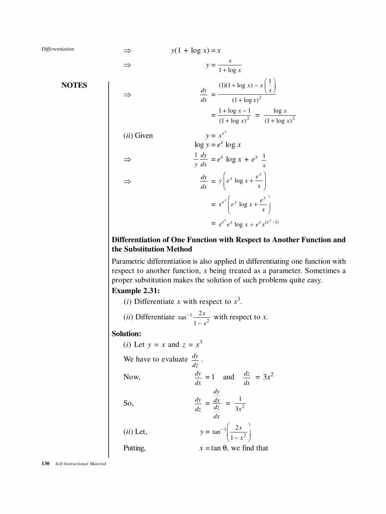
130 Self-Instructional Material
Differentiation
NOTES
⇒ y(1 + log x) = x
⇒ y =x
x1 + log
⇒dy
dx=
( )( log )
( log )
1 1
1 2
+ −1FHGIKJ
+
x xx
x
=1 1
1 2
+ −
+
log
( log )
x
x =
log
( log )
x
x1 2+
(ii) Given y = xe
x
log y = ex log x
⇒1
y
dy
dx= e
x log x + ex 1
x
⇒dy
dx= y e x
e
x
x
x
log +FHG
IKJ
= x e xe
x
e x
xx
log +FHG
IKJ
= ( 1)logx x
e x x ex e x e x
−+
Differentiation of One Function with Respect to Another Function and
the Substitution Method
Parametric differentiation is also applied in differentiating one function with
respect to another function, x being treated as a parameter. Sometimes a
proper substitution makes the solution of such problems quite easy.
Example 2.31:
(i) Differentiate x with respect to x3.
(ii) Differentiate 1
2
2tan
1
x
x
−
− with respect to x.
Solution:
(i) Let y = x and z = x3
We have to evaluate dy
dz.
Now,dy
dx= 1 and
dz
dx = 3x
2
So,dy
dz=
dy
dx
dz
dx
= 1
3 2x
(ii) Let, y = tan−
−
FHGIKJ
1
2
2
1
x
x
Putting, x = tan θ, we find that
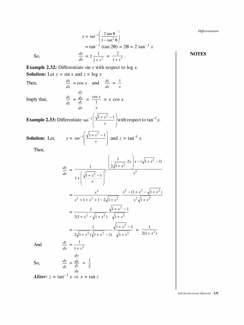
Differentiation
NOTES
Self-Instructional Material 131
y = tantan
tan
−
−
FHG
IKJ
1
2
2
1
θ
θ
= tan– 1 (tan 2θ) = 2θ = 2 tan– 1x
So,dy
dx= 2
1
12+ x
= 2
12+ x
.
Example 2.32: Differentiate sin x with respect to log x.
Solution: Let y = sin x and z = log x
Then,dy
dx= cos x and
dz
dx =
1
x
Imply that,dy
dz=
dy
dx
dz
dx
= cos x
x
1 = x cos x.
Example 2.33: Differentiate
21 1 1
tanx
x
− + −
with respect to tan–1x.
Solution: Let, y = tan− + −F
HGG
I
KJJ
121 1x
x and z = tan–1
x
Then,
dy
dx=
2
2
2 2
12 ( 1 1)
2 11.
1 11
x x x
x
xx
x
2
− + − +
+ − +
=x
x x x
x x x
x x
2
2 2 2
2 2 2
2 21 1 2 1
1 1
1+ + + − +⋅
− + − +
+
( )
=1
2 1 1
1 1
12 2
2
2( )+ − +
+ −
+x x
x
x
=1
2 1 1 1
1 1
12 2
2
2+ + −
+ −
+x x
x
x( ) =
1
2 1 2( )+ x
Anddz
dx=
1
1 2+ x
So,dy
dz=
dy
dx
dz
dx
= 1
2
Aliter: z = tan– 1x ⇒ x = tan z
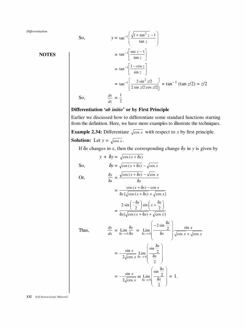
132 Self-Instructional Material
Differentiation
NOTES
So, y =2
1 1 tan 1tan
tan
z
z
− + −
= tansec
tan
− −LNM
OQP
1 1z
z
= tancos
sin
− −LNM
OQP
1 1 z
z
=2
1 2 sin /2tan
2 sin /2 cos /2
z
z z
−
= tan– 1 (tan z/2) = z/2
So,dy
dz=
1
2
Differentiation ‘ab initio’ or by First Principle
Earlier we discussed how to differentiate some standard functions starting
from the definition. Here, we have more examples to illustrate the techniques.
Example 2.34: Differentiate cos x with respect to x by first principle.
Solution: Let y = cos x .
If δx changes in x, then the corresponding change δy in y is given by
y + δy = cos ( )x x+ δ
So, δy = cos ( ) cosx x x+ −δ
Or,δ
δ
y
x=
cos ( ) cosx x x
x
+ −δ
δ
=cos ( ) cos
[ cos ( ) cos ]
x x x
x x x x
+ −
+ +
δ
δ δ
=
22 2
sin sin
[ cos ( ) cos ]
−FHGIKJ +FHG
IKJ
+ +
δ δ
δ δ
xx
x
x x x x
Thus,dy
dx=
0Limx
y
xδ →
δ
δ =
0
2 sinsin2Lim .
cos cosx
x
x
x x xδ →
δ −
δ +
=0
sinsin 2Lim
2 cos
2
x
x
x
xx δ →
δ
− δ
=0
sinsin 2as Lim
2 cos
2
x
x
x
xx δ →
δ
− δ
= 1.
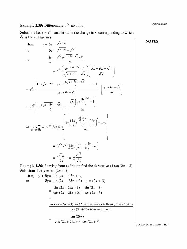
Differentiation
NOTES
Self-Instructional Material 133
Example 2.35: Differentiate ex ab initio.
Solution: Let y = ex and let δx be the change in x, corresponding to which
δy is the change in y.
Then, y + δy = ex x+ δ
⇒ δy = e ex x x+
−δ
⇒ δ
δ
y
x=
( 1)x x xx
e e
x
+ δ −−
δ
=1
x x x
xx x xe
exx x x
δ δ
δδ
+ − + −− + −
= e
x x xx x x
x x x
x
12
1
2
+ + − ++ −
+ −LNMM
OQPP
+ −
( )( )
!...δ
δ
δ
x x x
x
+ δ −
δ
= ex x x
xx
x
x
x 12
1 1
1 2
++ −
+LNMM
OQPP
+FHGIKJ −
LNMM
OQPP( )
!...
/
δ
δ
δ
⇒0
Limx
y
xδ →
δ
δ=
2
0
1 11
1 2 21 ... 1
2 2!( ) Limx
x
x x
x xe x
xδ →
− δ δ + + + −
δ
=20
1 1 1( ) Lim ...
2 8
x
x
xe x
x xδ →
δ − +
=e x
x
x
2 =
x
ex
2
1
Example 2.36: Starting from definition find the derivative of tan (2x + 3).
Solution: Let y = tan (2x + 3)
Then, y + δy = tan (2x + 2δx + 3)
⇒ δy = tan (2x + 2δx + 3) – tan (2x + 3)
= sin (2 2δ 3) sin (2 3)
cos (2 2δ 3) cos (2 3)
x x x
x x x
+ + +−
+ + +
=
sin (2 2δ 3)cos(2 3) sin (2 3)cos(2 2δ 3)
cos(2 2δ 3)cos(2 3)
x x x x x x
x x x
+ + + − + + +
+ + +
=sin (2δ )
cos (2 2δ 3) cos(2 3)
x
x x x+ + +
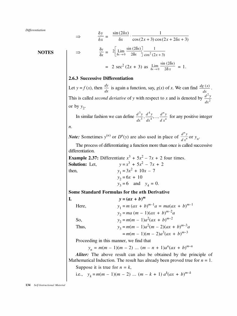
134 Self-Instructional Material
Differentiation
NOTES
⇒δ
δ
y
x=
sin (2δ ) 1
δ cos (2 3) cos (2 2δ 3)
x
x x x x⋅
+ + +
⇒y
x
δ
δ= 20
sin (2 ) 12 Lim
2 cos (2 3)x
x
x xδ →
δ δ +
= 2 sec2 (2x + 3) as 0
sin (2 )Lim
2x
x
xδ →
δ
δ = 1.
2.6.3 Successive Differentiation
Let y = f (x), then dy
dx is again a function, say,, g(x) of x. We can find
( )dg x
dx.
This is called second deriative of y with respect to x and is denoted by d y
dx
2
2
or by y2.
In similar fashion we can define d y
dx
d y
dx
3
3
4
4, ,
d y
d x
n
n..., for any positive integer
n.
Note: Sometimes y(n) or Dn(y) are also used in place of n
n
d y
d xor y
n.
The process of differentiating a function more than once is called successive
differentiation.
Example 2.37: Differentiate x3 + 5x
2 – 7x + 2 four times.
Solution: Let, y = x3 + 5x
2 – 7x + 2
then, y1
= 3x2 + 10x – 7
y2
= 6x + 10
y3
= 6 and y4 = 0.
Some Standard Formulas for the nth Derivative
I. y = (ax + b)m
Here, y1
= m (ax + b)m–1a = ma(ax + b)m–1
y2
= ma (m – 1)(ax + b)m–2a
So, y2
= m(m – 1)a2(ax + b)m–2
Thus, y3
= m(m – 1)a2(m – 2)(ax + b)m–3a
= m(m – 1)(m – 2)a3(ax + b)m–3
Proceeding in this manner, we find that
yn = m(m – 1)(m – 2) ... (m – n + 1)an(ax + b)m–n
Aliter: The above result can also be obtained by the principle of
Mathematical Induction. The result has already been proved true for n = 1.
Suppose it is true for n = k,
i.e., yk
= m(m – 1)(m – 2) ... (m – k + 1) ak(ax + b)m–k
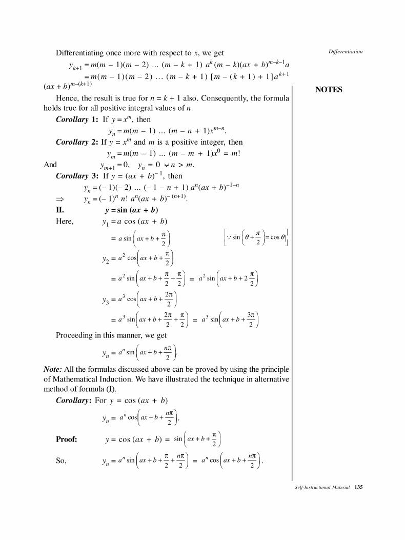
Differentiation
NOTES
Self-Instructional Material 135
Differentiating once more with respect to x, we get
yk+1
= m(m – 1)(m – 2) ... (m – k + 1) ak (m – k)(ax + b)m–k–1
a
= m(m – 1)(m – 2) . . . (m – k + 1) [m – (k + 1) + 1]ak+1
(ax + b)m–(k+1)
Hence, the result is true for n = k + 1 also. Consequently, the formula
holds true for all positive integral values of n.
Corollary 1: If y = xm, then
yn
= m(m – 1) ... (m – n + 1)xm–n.
Corollary 2: If y = xm and m is a positive integer, then
ym
= m(m – 1) ... (m – m + 1)x0 = m!
And ym+1
= 0, yn = 0 ∨− n > m.
Corollary 3: If y = (ax + b)– 1, then
yn
= (– 1)(– 2) ... (– 1 – n + 1) an(ax + b)–1–n
⇒ yn
= (– 1)n n! an(ax + b)– (n+1).
II. y = sin (ax + b)
Here, y1
= a cos (ax + b)
= sin + +2
a ax bπ
sin cos2
πθ θ
+ =
∵
y2
= a ax b2
2cos + +FHG
IKJ
π
= a ax b2
2 2sin + + +FHG
IKJ
π π = a ax b
2 22
sin + +FHG
IKJ
π
y3
= a ax b3 2
2cos + +FHG
IKJ
π
= a ax b3 2
2 2sin + + +FHG
IKJ
π π = a ax b
3 3
2sin + +FHG
IKJ
π
Proceeding in this manner, we get
yn
= sin .2
n na ax b
π + +
Note: All the formulas discussed above can be proved by using the principle
of Mathematical Induction. We have illustrated the technique in alternative
method of formula (I).
Corollary: For y = cos (ax + b)
yn
= a ax bnn cos + +
FHG
IKJ
π
2.
Proof: y = cos (ax + b) = sin2
ax bπ
+ +
So, yn
= a ax bnn sin + + +
FHG
IKJ
π π
2 2 = a ax b
nn cos + +FHG
IKJ
π
2.
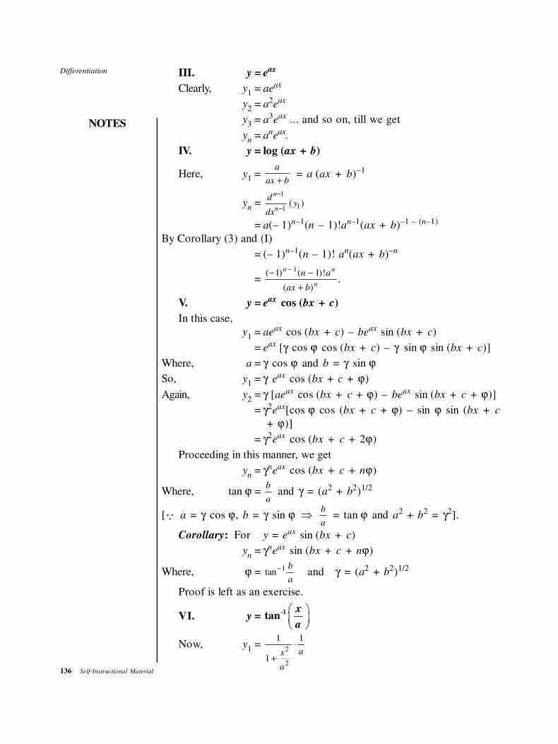
136 Self-Instructional Material
Differentiation
NOTES
III. y = eax
Clearly, y1
= aeax
y2
= a2e
ax
y3
= a3e
ax ... and so on, till we get
yn
= ane
ax.
IV. y = log (ax + b)
Here, y1
=a
ax b+ = a (ax + b)–1
yn
=1
11( )
n
n
dy
dx
−
−
= a(– 1)n–1(n – 1)!an–1(ax + b)–1 – (n–1)
By Corollary (3) and (I)
= (– 1)n–1(n – 1)! an(ax + b)–n
=( ) ( )!
( )
− −
+
−1 11n n
n
n a
ax b.
V. y = eax cos (bx + c)
In this case,
y1
= aeax cos (bx + c) – be
ax sin (bx + c)
= eax [γ cos ϕ cos (bx + c) – γ sin ϕ sin (bx + c)]
Where, a = γ cos ϕ and b = γ sin ϕ
So, y1
= γ eax cos (bx + c + ϕ)
Again, y2
= γ [aeax cos (bx + c + ϕ) – be
ax sin (bx + c + ϕ)]
= γ2e
ax[cos ϕ cos (bx + c + ϕ) – sin ϕ sin (bx + c
+ ϕ)]
= γ2e
ax cos (bx + c + 2ϕ)
Proceeding in this manner, we get
yn
= γne
ax cos (bx + c + nϕ)
Where, tan ϕ =b
a and γ = (a2 + b
2)1/2
[∵ a = γ cos ϕ, b = γ sin ϕ ⇒b
a = tan ϕ and a
2 + b2 = γ2].
Corollary: For y = eax sin (bx + c)
yn
= γne
ax sin (bx + c + nϕ)
Where, ϕ = tan−1 b
aand γ = (a2 + b
2)1/2
Proof is left as an exercise.
VI. y =
-1tan
x
a
Now, y1
=1
1
12
2+
⋅x
a
a
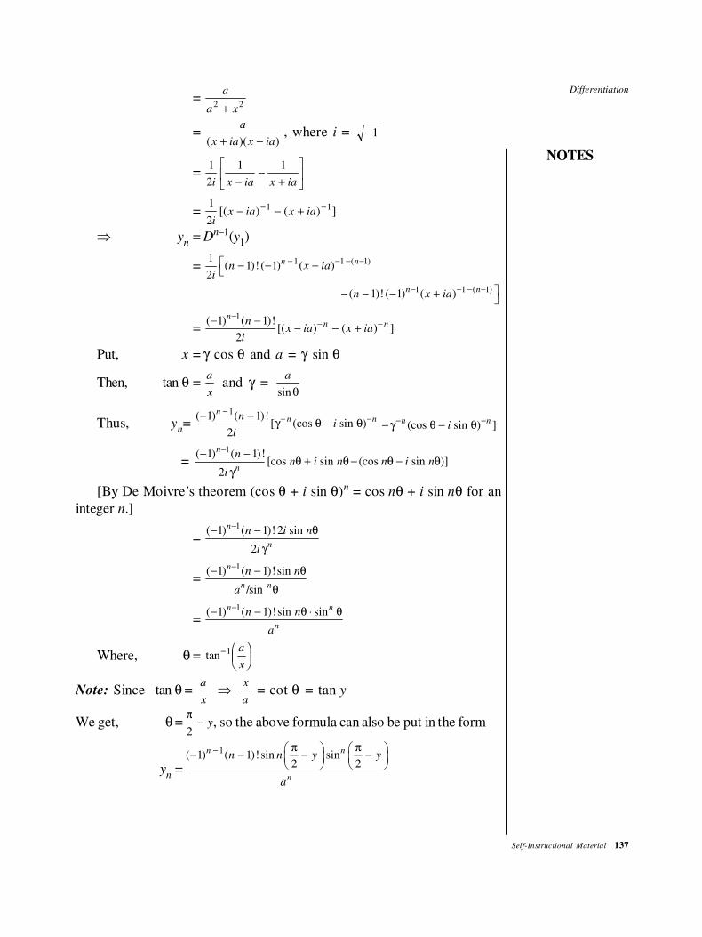
Differentiation
NOTES
Self-Instructional Material 137
=a
a x2 2+
=a
x ia x ia( )( )+ −, where i = −1
=1
2
1 1
i x ia x ia−−
+
LNM
OQP
=1
2
1 1
ix ia x ia[( ) ( ) ]− − +− −
⇒ yn
= Dn–1(y
1)
= 1 1 ( 1)1( 1)! ( 1) ( )
2
n nn x ia
i
− − − − − − −
1 1 ( 1)( 1)! ( 1) ( )n nn x ia
− − − − − − − +
=1
( 1) ( 1)![( ) ( ) ]
2
nn nn
x ia x iai
−− −− −
− − +
Put, x = γ cos θ and a = γ sin θ
Then, tan θ =a
x and γ =
a
sinθ
Thus, yn=
1( 1) ( 1)!
[ (cos sin )2
nn nn
ii
−− −− −
γ θ − θ (cos sin ) ]n n
i− −− γ θ − θ
=1( 1) ( 1)!
[cos sin (cos sin )]2
n
n
nn i n n i n
i
−− −θ + θ − θ − θ
γ
[By De Moivre’s theorem (cos θ + i sin θ)n = cos nθ + i sin nθ for an
integer n.]
=1( 1) ( 1)! 2 sin
2
n
n
n i n
i
−− − θ
γ
=1( 1) ( 1)!sin
/sin
n
n n
n n
a
−− − θ
θ
=1( 1) ( 1)! sin sinn n
n
n n
a
−− − θ ⋅ θ
Where, θ = tan− FHGIKJ
1 a
x
Note: Since tan θ = a
x⇒
x
a = cot θ = tan y
We get, θ =π
2− y, so the above formula can also be put in the form
yn
=
1( 1) ( 1)! sin sin
2 2
n n
n
n n y y
a
− π π − − − −
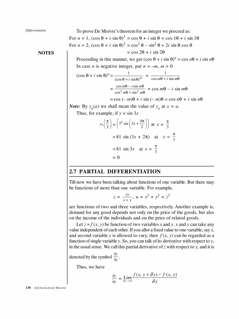
138 Self-Instructional Material
Differentiation
NOTES
To prove De Moivre’s theorem for an integer we proceed as:
For n = 1, (cos θ + i sin θ)1 = cos θ + i sin θ = cos 1θ + i sin 1θ
For n = 2, (cos θ + i sin θ)2 = cos2 θ – sin2 θ + 2i sin θ cos θ
= cos 2θ + i sin 2θ
Proceeding in this manner, we get (cos θ + i sin θ)n = cos nθ + i sin nθ
In case n is negative integer, put n = –m, m > 0
(cos θ + i sin θ)n =1
(cos sin )θ θ+ im
= 1
cos sinm i mθ θ+
=cos sin
cos sin
m i m
m m
θ θ
θ θ
−
+2 2 = cos mθ – i sin mθ
= cos (– m)θ + i sin (– m)θ = cos nθ + i sin nθ
Note: By yn(a) we shall mean the value of y
n at x = a.
Thus, for example, if y = sin 3x
43
yπ
=4 4
3 sin 32
x π
+
at x = 3
π
= 81 sin (3x + 2π) at x = 3
π
= 81 sin 3x at x = 3
π
= 0
2.7 PARTIAL DIFFERENTIATION
Till now we have been talking about functions of one variable. But there may
be functions of more than one variable. For example,
z = xy
x y+, u = x
2 + y2 + z
2
are functions of two and three variables, respectively. Another example is,
demand for any good depends not only on the price of the goods, but also
on the income of the individuals and on the price of related goods.
Let z = f (x, y) be function of two variables x and y. x and y can take any
value independent of each other. If you allot a fixed value to one variable, say x,
and second variable y is allowed to vary, then f (x, y) can be regarded as a
function of single variable y. So, you can talk of its derivative with respect to y,
in the usual sense. We call this partial derivative of z with respect to y, and it is
denoted by the symbol ∂
∂
z
y.
Thus, we have
∂
∂
z
y=
0
( , ) ( , )Limy
f x y y f x y
yδ
δ
δ→
+ −
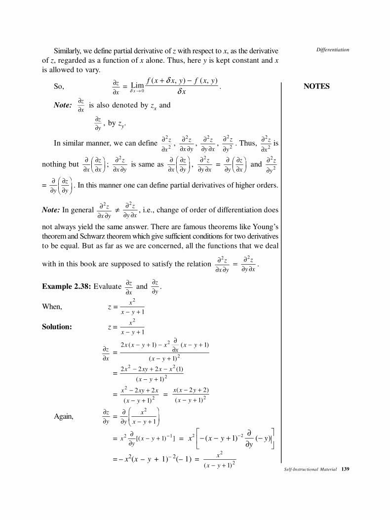
Differentiation
NOTES
Self-Instructional Material 139
Similarly, we define partial derivative of z with respect to x, as the derivative
of z, regarded as a function of x alone. Thus, here y is kept constant and x
is allowed to vary.
So,∂
∂
z
x=
0
( , ) ( , )Lim
x
f x x y f x y
xδ
δ
δ→
+ −.
Note:z
x
∂
∂ is also denoted by z
x and
z
y
∂
∂, by z
y.
In similar manner, we can define ∂
∂
2
2
z
x
, ∂
∂ ∂
2z
x y,
∂
∂ ∂
2z
y x,
∂
∂
2
2
z
y
. Thus, ∂
∂
2
2
z
x
is
nothing but ∂
∂
∂
∂
FHGIKJx
z
x;
∂
∂ ∂
2z
x y is same as
∂
∂
∂
∂
FHGIKJx
z
y,
∂
∂ ∂
2z
y x =
∂
∂
∂
∂
FHGIKJy
z
x and
∂
∂
2
2
z
y
= ∂
∂
∂
∂
FHGIKJy
z
y. In this manner one can define partial derivatives of higher orders.
Note: In general ∂
∂ ∂
2z
x y ≠
∂
∂ ∂
2z
y x, i.e., change of order of differentiation does
not always yield the same answer. There are famous theorems like Young’s
theorem and Schwarz theorem which give sufficient conditions for two derivatives
to be equal. But as far as we are concerned, all the functions that we deal
with in this book are supposed to satisfy the relation ∂
∂ ∂
2z
x y =
∂
∂ ∂
2z
y x.
Example 2.38: Evaluate ∂
∂
z
x and
∂
∂
z
y.
When, z =x
x y
2
1− +
Solution: z =x
x y
2
1− +
z
x
∂
∂=
2 1 1
1
2
2
x x y xx
x y
x y
( ) ( )
( )
− + −∂
∂− +
− +
=2 2 2 1
1
2 2
2
x xy x x
x y
− + −
− +
( )
( )
=x xy x
x y
2
2
2 2
1
− +
− +( ) =
x x y
x y
( )
( )
− +
− +
2 2
1 2
Again,∂
∂
z
y=
∂
∂ − +
FHG
IKJy
x
x y
2
1
= xy
x y2 11
∂
∂− + −[( ) ] =
2 2( 1) ( )x x y yy
− ∂− − + − ∂
= – x2(x – y + 1)– 2(– 1) =
x
x y
2
21( )− +
140 Self-Instructional Material
Differentiation
NOTES
Example 2.39: Verify that for z = log (x2 – y
2).
∂
∂ ∂
2z
x y=
∂
∂ ∂
2z
y x.
Solution:∂
∂
z
x=
∂
∂x [log (x2 – y2)] =
22 2
x
x y−
∂
∂ ∂
2z
y x= 2 2
2x
y x y
∂ ∂ −
= 2 2 1
2 [( ) ]x x yy
−∂−
∂
=2 2 2 22 ( ) ( )x x y y
y
− ∂− − − ∂
= – 2x(x2 – y2)– 2(– 2y) =
+
−
42 2 2
xy
x y( )...(1)
Further,∂
∂
z
y=
∂
∂−
yx y[log ( )]2 2 =
−
−
22 2
y
x y
∂
∂ ∂
2z
x y=
∂
∂−
−
LNMM
OQPPx
y
x y
22 2
= ( ) [( ) ]−∂
∂− −2 2 2 1
yx
x y
= ( ) ( ) ( )− − −∂
∂
LNM
OQP
−2 2 2 2 2y x y
xx =
42 2 2
xy
x y( )−...(2)
Equations (1) and (2) give the required result.
Example 2.40: Show that 2
[( ) ]+∂
+∂ ∂
x yx y e
x y = (x + y + 2)ex+y.
Solution: ( ) x yx y e
y
+∂ + ∂
= [ ( )]x y
e e x yy
∂+
∂
= ex[ey(x + y) + ey]
= exe
y(x + y + 1)
2
( )x y
x y ex y
+∂ + ∂ ∂
=∂
∂x[ex
ey(x + y + 1)]
= [ ( 1)]y x
e e x yx
∂+ +
∂
= ey[ex(x + y + 1) + e
x]
= exe
y(x + y + 1 + 1)
= ex+y(x + y + 2)
= (x + y + 2) ex+y
Example 2.41: If u = log (x2 + y
2 + z
2), prove that:
xu
y z
∂
∂ ∂
2
= yu
z x
∂
∂ ∂
2
= zu
x y
∂
∂ ∂
2
.
Solution: u = log (x2 + y2 + z2)
Differentiation
NOTES
Self-Instructional Material 141
⇒ ∂
∂
u
x=
d
d x y z
x y zx y z
x( )[log ( )]
( )2 2 2
2 2 22 2 2
+ ++ +
∂ + +
∂
=1
22 2 2
x y z
x
+ +⋅ =
22 2 2
x
x y z+ +
⇒ ∂
∂ ∂
2u
z x=
∂
∂
∂
∂
FHGIKJz
u
x =
2 2 2 2
2. (2 )
( )−
+ +
xz
x y z =
−
+ +
42 2 2 2
xz
x y z( )
⇒ yu
z x
∂
∂ ∂
2
= −
+ +
42 2 2 2
xyz
x y z( )...(1)
Again,∂
∂ ∂
2u
x y=
∂
∂ ∂
2u
y x =
∂
∂
∂
∂
LNMOQPy
u
x
= −+ +
22
2 2 2 2
x
x y z
y
( )( ) =
−
+ +
42 2 2 2
xy
x y z( )
⇒ z∂
∂ ∂
2u
x y= −
+ +
42 2 2 2
xyz
x y z( )...(2)
Similarly, it can be shown that
xu
y z
∂
∂ ∂
2
= −+ +
42 2 2 2
xyz
x y z( )...(3)
Equations (1), (2) and (3) give the required result.
Example 2.42: If u = f (r), where r = x y2 2+ ,
prove that ∂
∂+
∂
∂
2
2
2
2
u
x
u
y
= f′′ (r) + ( )′1
f rr
.
Solution: r = (x2 + y2)1/2
⇒∂
∂
r
x=
1
222 2 1 2⋅ + ⋅−( ) /
x y x = x
x y2 2+
= x
r
Similarly,∂
∂
r
y=
y
r.
Now, u = f (r)
⇒∂
∂
u
x=
d
dru
r
x( )
∂
∂
⇒ =′u x
r where u′ =
du
dr = f ′(r)
⇒∂
∂
2
2
u
x
=u
r
x
r
u
xu x
x r
′+
∂ ′
∂+ ′
∂
∂
FHGIKJ
1
=u
r
x
r
d
dru
r
xxu
d
dx r
r
x
′+ ′
∂
∂+ ′
FHGIKJ
∂
∂( )
1
142 Self-Instructional Material
Differentiation
NOTES
=u
r
x
r
u′
+ ′2
2
xu
r
x
r′ −
′2
where u′′ = d u
dr
2
2 = f ′′(r)
=2 2
2 3
′ ′′+ − ′
u x u xu
r r r.
In a similar manner, it can be proved that:
∂
∂
2
2
u
y
=2 2
2 3
′ ′′+ − ′
u y u yu
r r r
So,∂
∂
2
2
u
x
+ ∂
∂
2
2
u
y
= 2 2 2 2
2 3
2( ) ( )
′ ′′ ′+ + − +
u u ux y x y
r r r
= 2 2
2 3
2 ′ ′′ ′+ ⋅ − ⋅
u u ur r
r r r=
2 ′ ′+ ′′ −
u uu
r r
=u
ur
′′′ + =
1( ) ( ).′′ + ′f r f r
r
2.8 MAXIMA AND MINIMA OF FUNCTIONS
Definition 1
The point (c, f (c)) is called a maximum point of y = f (x), if (i) f (c + h) ≤ f (c),
and (ii) f (c – h) ≤ f (c) for small h ≥ 0. f (c) itself is called a maximum value of
f (x).
Definition 2
The point (d, f (d)) is called a minimum point of y = f (x), if
(i) f (d +h) ≥ f (d), and
(ii) f (d – h) ≥ f (d)
for all small h ≥ 0.
f (d) itself is called a minimum value of f (x).
Thus, you observe that points P [c – h, f (c – h)] and Q [c + h, f (c + h)], which
are very near to A, have ordinates less than that of A, whereas the points
R[d – h, f (d – h)], and S [d + h, f (d + h)],
Which are very close to B, have ordinates greater than that of B.
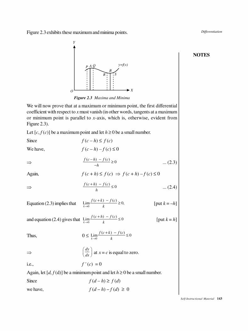
Differentiation
NOTES
Self-Instructional Material 143
Figure 2.3 exhibits these maximum and minima points.
O X
Y
P A Q
R S
B
y=f(x)
Figure 2.3 Maxima and Minima
We will now prove that at a maximum or minimum point, the first differential
coefficient with respect to x must vanish (in other words, tangents at a maximum
or minimum point is parallel to x-axis, which is, otherwise, evident from
Figure 2.3).
Let [c, f (c)] be a maximum point and let h ≥ 0 be a small number.
Since f (c – h) ≤ f (c)
We have, f (c – h) – f (c) ≤ 0
⇒( ) ( )
0f c h f c
h
− −≥
−... (2.3)
Again, f (c + h) ≤ f (c) ⇒ f (c + h) – f (c) ≤ 0
⇒( ) ( )
0f c h f c
h
+ −≤ ... (2.4)
Equation (2.3) implies that0
( ) ( )Lim 0,k
f c k f c
k→
+ −≥ [put k = –h]
and equation (2.4) gives that0
( ) ( )Lim 0k
f c h f c
k→
+ −≤ [put k = h]
Thus, 0 ≤ 0
( ) ( )Lim 0k
f c k f c
k→
+ −≤
⇒dy
dx
at x = c is equal to zero.
i.e., f ' (c) = 0
Again, let [d, f (d)] be a minimum point and let h ≥ 0 be a small number.
Since f (d – h) ≥ f (d)
we have, f (d – h) – f (d) ≥ 0
144 Self-Instructional Material
Differentiation
NOTES
⇒ ( ) ( )
0f d h f d
h
− −≤
−... (2.5)
Again, f (d + h) ≥ f (d)
⇒( ) ( )
0f d h f d
h
+ −≥ ... (2.6)
Equations (2.5) and (2.6) imply0
( ) ( )Lim 0k
f d k f d
k→
+ −=
i.e., f ' (d) = 0
Before we proceed to find out the criterion for determining whether a point is
maximum or minimum, we will discuss the increasing and decreasing functions
of x.
A function f(x) is said to be increasing (decreasing) if
f (x + c) ≥ f (x) ≥ f (x – c) [ f (x + c) ≤ f (x) ≤ f (x – c)] for all c ≥ 0.
Theorem 2.1
If f '(x) ≥ 0, then f (x) is increasing function of x and if f '(x) ≤ 0, then f(x) is
decreasing function of x.
Proof: f ' (x) ≥ 0 ⇒ 0
( ) ( )Lim 0x
f x x f x
xδ →
+ δ −≥
δ... (2.7)
In case δx > 0, put c = δx, then equation (2.7) gives
f(x + c) ≥ f(x)
In case δx < 0, put c = – δx, then equation (2.7) gives
( ) ( )0
f x c f x
c
− −≥
−
⇒ f (x – c) – f (x) ≤ 0
⇒ f (x) ≥ f (x – c)
Hence, f (x + c) ≥ f (x) ≥ f (x – c)
In other words, f (x) is increasing function of x.
Suppose that f ' (x) ≤ 0
Then,0
( ) ( )Lim 0x
f x x f x
xδ →
+ δ −≤
δ... (2.8)
In case δx > 0, put c = δx, then Equation (2.8) gives
f (x + c) – f (c) ≤ 0
i.e., f (x + c) ≤ f (x)
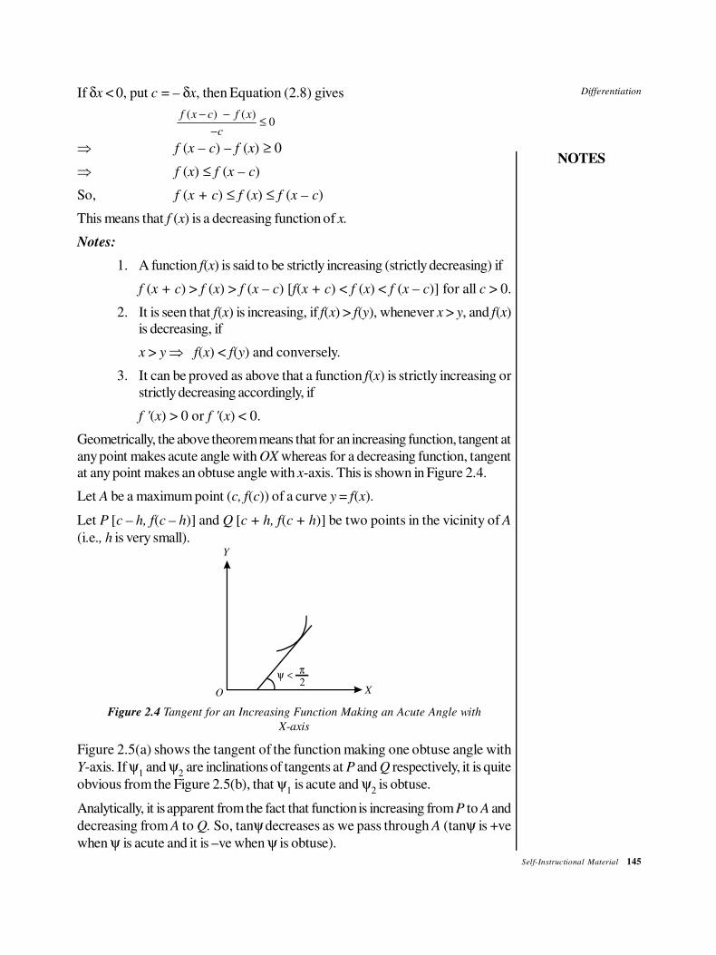
Differentiation
NOTES
Self-Instructional Material 145
If δx < 0, put c = – δx, then Equation (2.8) gives
( ) ( )0
f x c f x
c
− −≤
−
⇒ f (x – c) – f (x) ≥ 0
⇒ f (x) ≤ f (x – c)
So, f (x + c) ≤ f (x) ≤ f (x – c)
This means that f (x) is a decreasing function of x.
Notes:
1. A function f(x) is said to be strictly increasing (strictly decreasing) if
f (x + c) > f (x) > f (x – c) [f(x + c) < f (x) < f (x – c)] for all c > 0.
2. It is seen that f(x) is increasing, if f(x) > f(y), whenever x > y, and f(x)
is decreasing, if
x > y ⇒ f(x) < f(y) and conversely.
3. It can be proved as above that a function f(x) is strictly increasing or
strictly decreasing accordingly, if
f '(x) > 0 or f '(x) < 0.
Geometrically, the above theorem means that for an increasing function, tangent at
any point makes acute angle with OX whereas for a decreasing function, tangent
at any point makes an obtuse angle with x-axis. This is shown in Figure 2.4.
Let A be a maximum point (c, f(c)) of a curve y = f(x).
Let P [c – h, f(c – h)] and Q [c + h, f(c + h)] be two points in the vicinity of A
(i.e., h is very small).
ψ < π2
O X
Y
Figure 2.4 Tangent for an Increasing Function Making an Acute Angle with
X-axis
Figure 2.5(a) shows the tangent of the function making one obtuse angle with
Y-axis. If ψ1 and ψ
2 are inclinations of tangents at P and Q respectively, it is quite
obvious from the Figure 2.5(b), that ψ1 is acute and ψ
2 is obtuse.
Analytically, it is apparent from the fact that function is increasing from P to A and
decreasing from A to Q. So, tanψ decreases as we pass through A (tanψ is +ve
when ψ is acute and it is –ve when ψ is obtuse).
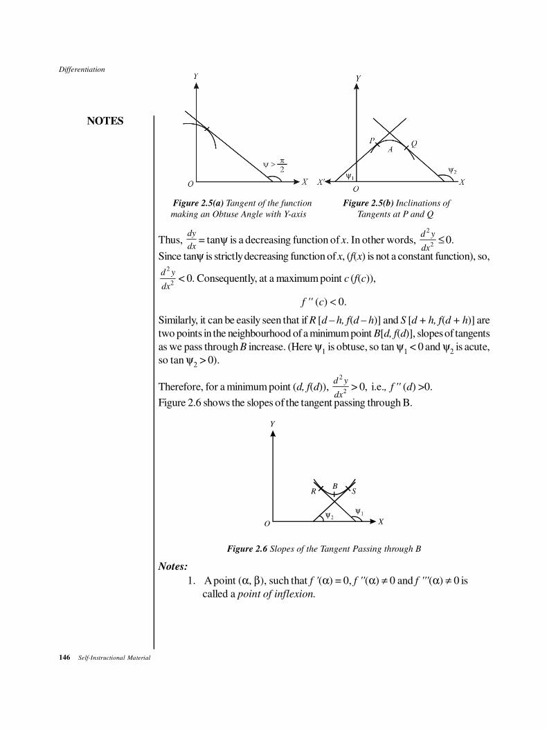
146 Self-Instructional Material
Differentiation
NOTES
Y
Figure 2.5(a) Tangent of the function Figure 2.5(b) Inclinations of
making an Obtuse Angle with Y-axis Tangents at P and Q
Thus, dy
dx= tanψ is a decreasing function of x. In other words,
2
2
d y
dx≤ 0.
Since tanψ is strictly decreasing function of x, (f(x) is not a constant function), so,2
2
d y
dx< 0. Consequently, at a maximum point c (f(c)),
f '' (c) < 0.
Similarly, it can be easily seen that if R [d – h, f(d – h)] and S [d + h, f(d + h)] are
two points in the neighbourhood of a minimum point B[d, f(d)], slopes of tangents
as we pass through B increase. (Here ψ1 is obtuse, so tan ψ
1 < 0 and ψ
2 is acute,
so tan ψ2 > 0).
Therefore, for a minimum point (d, f(d)), 2
2
d y
dx> 0, i.e., f '' (d) >0.
Figure 2.6 shows the slopes of the tangent passing through B.
O X
Y
ψ2ψ1
R SB
Figure 2.6 Slopes of the Tangent Passing through B
Notes:
1. A point (α, β), such that f '(α) = 0, f ''(α) ≠ 0 and f '''(α) ≠ 0 is
called a point of inflexion.
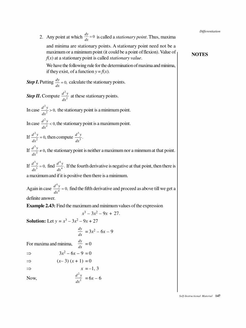
Differentiation
NOTES
Self-Instructional Material 147
2. Any point at which 0dy
dx= is called a stationary point. Thus, maxima
and minima are stationary points. A stationary point need not be a
maximum or a minimum point (it could be a point of flexion). Value of
f(x) at a stationary point is called stationary value.
We have the following rule for the determination of maxima and minima,
if they exist, of a function y = f(x).
Step I. Putting 0,dy
dx= calculate the stationary points.
Step II. Compute 2
2
d y
dx at these stationary points.
In case 2
20,
d y
dx> the stationary point is a minimum point.
In case 2
20,
d y
dx< the stationary point is a maximum point.
If 2
20
d y
dx= , then compute
3
3.
d y
dx
If 3
30
d y
dx≠ , the stationary point is neither a maximum nor a minmum at that point.
If 3
30,
d y
dx= find
4
4.
d y
dx If the fourth derivative is negative at that point, then there is
a maximum and if it is positive then there is a minimum.
Again in case 4
40,
d y
dx= find the fifth derivative and proceed as above till we get a
definite answer.
Example 2.43: Find the maximum and minimum values of the expression
x3 – 3x2 – 9x + 27.
Solution: Let y = x3 – 3x2 – 9x + 27
dy
dx= 3x2 – 6x – 9
For maxima and minima,dy
dx= 0
⇒ 3x2 – 6x – 9 = 0
⇒ (x– 3) (x + 1) = 0
⇒ x = –1, 3
Now,2
2
d y
dx= 6x – 6
148 Self-Instructional Material
Differentiation
NOTES
At x = –1, 2
212 0,
d y
dx
= − < so x = –1 gives a maximum point of y.
Again, at x = 3, 2
212 0,
d y
dx
= + > x = 3 gives a minimum point of y.
Hence, maximum value of y is [(–1)3 – 3 (–1)2 – 9 (–1) + 27]
= 36 + 1 – 3 = 34
While minimum value of y is 33 – 3(3)2 – 9 (3) + 27
= 54 – 27 – 27 = 0
Example 2.44: Find the maximum and minimum values of the function
8x5 – 15x4 + 10x2.
Solution: Let f(x) = 8x5 – 15x4 + 10x2
⇒ f ′(x) = 40x4 – 60x3 + 20x
For maxima and minima,
f ′(x) = 0 ⇒ x = 0, 1, –2
1
So, these are the points where there can be a maximum or a minimum
Now, f ′′(x) = 160x3 – 180x2 + 20
Thus, f ′′(0) = 20 > 0 ⇒ There is a minimum at x = 0
Again, f ′′(–2
1) = 160 (–
2
1)3 – 180 (–
2
1)2 + 20 = –45 < 0
⇒ there is a maximum at x = –2
1
Since f ′′(1) = 160 – 180 + 20 = 0, we cannot say anything regarding a maximum
or a minimum at x = 1 at this stage. So, we find f ′′′(x).
Now, f ′′′(x) = 480 x2 – 360 x
But, f ′′′(1) = 480 – 360 ≠ 0
⇒ There is neither a maximum nor a minimum at x = 1
Hence, f (–2
1) =
16
21 is maximum value and f (0) = 0 is minimum value.
Example 2.45: Find out maxima and minima of sin x + cos x, when x lies between
0 and 2π.
Solution: Let y = sin x + cos x, 0 ≤ x ≤ 2π
For maxima and minima, dx
dy= 0
⇒ cos x – sin x = 0
⇒ tan x = 1
Differentiation
NOTES
Self-Instructional Material 149
⇒ x = 4
πor
4
3π.
Now, 2
2
dx
yd= – sin x – cos x
At,2
2
1 1,
4 2 2
d yx
dx
π= = − − = –√2 < 0
And at,2
2
3 1 1,
4 2 2
d yx
dx
π= = + = √2 > 0
So, x = 4
π gives a maximum and x =
4
3πgives a minimum point of given
function.
Example 2.46: Find maxima and minima of
sin x + cos 2 x for 0 ≤ x ≤ π /2.
Solution: Let y = sin x + cos 2x
For maxima and minima dx
dy= 0
⇒ cos x – 2 sin 2x = 0
⇒ cos x(1 – 4 sin x) = 0
⇒ cos x = 0 or sin x = 4
1
⇒ x = 2
πor x = sin–1
4
1
Now, 2
2
dx
yd=–sin x – 4 cos 2x
=–sin x – 4 (1 – 2 sin2x)
=8 sin2x – sin x – 4
At, x = π/2, 2
2
dx
yd= 8 – 1 – 4 = 3 > 0
So, x = 2
π gives a minimum point of sin x + cos 2x
At, x =
21
2
1sin ,
4
d y
dx
−=
1 18 4
16 4
− −
=1 1
42 4
− −
150 Self-Instructional Material
Differentiation
NOTES
= 1 17 15
02 4 4
− = − <
Consequently, x = sin–1
4
1 gives a maximum point of sin x + cos 2x.
Example 2.47: The sum of two numbers is 24. Find the numbers if the sum of
their squares is to be minimum.
Solution: Let x and y be two numbers such that
x + y = 24
Let, s = x2+ y2 = x2 + (24 – x)2
For maxima and minima, dx
ds= 0
⇒ 2x – 2 (24 – x) = 0
⇒ 2x = 24 ⇒ x = 12
Further,2
2
d s
dx= 4 > 0
So, x = 12 and y = 12 give minimum value.
Hence, the required numbers are 12 and 12.
CHECK YOUR PROGRESS
7. What is parametric differentiation?
8. Determine dx
dy where x = a ( 1 + sin θ) and y = a (1 – cos θ).
9. When do we take help of logarithmic differentiation?
10. What is successive differentiation?
11. Find first four derivatives of y = x3 + 5x2 – 7x +2.
12. What do you understand by partial differentiation?
13. When is a point called maximum and has a maximum value?
14. When is a function f(x) said to be increasing or decreasing?
2.9 SUMMARY
In this unit, you have learned that:
• In mathematics, usually there are two kinds of quantities: constants and
variables.
• A quantity which is liable to vary is called a variable quantity or simply a
variable, and a quantity that retains its value through all mathematical
operations is termed as a constant quantity or a constant.
Differentiation
NOTES
Self-Instructional Material 151
• Limits of a function can be evaluated using the expansion method.
• The derivative of the sum (or difference) of two functions is equal to the
sum (or difference) of their derivatives.
• The derivative of a product of two functions = (the derivative of first function
× second function) + (first function × derivative of second function).
• The derivative of a constant function is equal to the constant multiplied by
the derivative of the function.
• The chain rule of differentiation states that if y is a differentiable function of
z, and z is a differentiable function of x, then y is a differentiable function
of x.
• Logarithms are used to find differential coefficients of functions which are
either product or quotient of functions whose differential coefficients are
known, or whose variables occur in powers.
• Parametric differentiation is also applied in differentiating one function with
respect to another function, x being treated as a parameter.
2.10 KEY TERMS
• Derivative: It refers to the instantaneous rate of change of a function.
• Variable: It refers to a quantity that is liable to vary.
• Constant: It refers to a quantity that retains its value through all mathematical
operations.
• Differentiation: It refers to the rate of change of any quantity with respect
to the change in another quantity with which it has a functional relationship.
• Maxima: It refers to the largest value that a function takes in a point either
within a given neighbourhood or on the function domain in its entirety.
• Minima: It refers to the smallest value that a function takes in a point either
within a given neighbourhood or on the function domain in its entirety.
2.11 ANSWERS TO ‘CHECK YOUR PROGRESS’
1.2
1
1Lim
1x
x
x→
−
− = 2.
2. 27.
3. A function f (x) is said to be derivable or differentiable at x = a if its deriva-tive exists at x = a.
152 Self-Instructional Material
Differentiation
NOTES
4. 6x – 6 and 5
24 5 2 5 7
2 3 2( )( )
/x x x+ + − .
5. The derivative of a product of two functions = (the derivative of first func-
tion × second function) + (first function × derivative of second function).
6. The chain rule is the most important and widely used rule for differentiation.
The rule states that if y is a differentiable function of z, and z is a
differentiable function of x, then y is a differentiable function of x.
7. When x and y are separately given as functions of a single variable t
(called a parameter), then we first evaluate dx
dt and
dy
dt and then use
chain formula dy
dt =
dy
dx
dx
dt, to obtain
dy
dx=
dy
dt
dx
dt
The equations x = F (t) and y = G(t) are called parametric equations.
8.dy
dx=
dy
d
dx
d
θ
θ
= sin /2
cos /2
θ
θ = tan
θ
2.
9. Whenever we have a function which is a product or quotient of functions
whose differential coefficients are known or a function, in which variables
occur in powers, we take the help of logarithms.
10. The process of differentiating a function more than once is calledsuccessive differentiation.
11. Let y = z3 + 5x
2 – 7x + 2
then, y1 = 3x
2 + 10x – 7
y2 = 6x + 10
y3 = 6 and
y4 = 0.
12. Let z = f (x, y) be function of two variables x and y. x and y can take any
value independently of each other. If we allot a fixed value to one variable,
say x, and second variable y is allowed to vary, f (x, y) can be regarded
as a function of single variable y. So we can talk of its derivative with
respect to y, in the usual sense. We call this partial derivative of z with
respect to y, and denote it by the symbol ∂
∂
z
y.
Differentiation
NOTES
Self-Instructional Material 153
Thus, we have,
∂
∂
z
y =
0
( , ) ( , )Limy
f x y y f x y
yδ
δ
δ→
+ −
Similarly, we define partial derivative of z with respect to x, as the
derivative of z, regarded as a function of x alone. Thus, here y is kept
constant and x is allowed to vary.
So, ∂
∂
z
x =
0
( , ) ( , )Lim
x
f x x y f x y
xδ
δ
δ→
+ −
In similar manner, we can define ∂
∂
2
2
z
x
, ∂
∂ ∂
2z
x y,
∂
∂ ∂
2z
y x,
∂
∂
2
2
z
y
. Thus, ∂
∂
2
2
z
x
is
nothing but ∂
∂
∂
∂
FHGIKJx
z
x;
∂
∂ ∂
2z
x y is same as
∂
∂
∂
∂
FHGIKJx
z
y,
∂
∂ ∂
2z
y x =
∂
∂
∂
∂
FHGIKJy
z
x and
∂
∂
2
2
z
y
= ∂
∂
∂
∂
FHGIKJy
z
y. In this manner one can define partial derivatives of
higher orders.
13. The point (c, f (c)) is called a maximum point of y = f (x), if (i) f
(c + h) ≤ f (c), and (ii) f (c – h) ≤ f (c) for small h ≥ 0. f (c) itself
is called a maximum value of f (x).
14. A function f(x) is said to be increasing (decreasing) if f (x + c) ≥ f (x) ≥
f (x – c) [ f (x + c) ≤ f (x) ≤ f (x – c)] for all c ≥ 0.
2.12 QUESTIONS AND EXERCISES
Short-Answer Questions
1. Evaluate 0
Sin 3Lim
Sin 5x
x
x→.
2. Differentiate with respect to x; y = sin3 x.
3. Differentiate with respect to x; y = log (sin x).
4. Find derivative y = log x from first principle (ab initio).
5. Find fifth derivative of y = x4.
6. Find maximum and minimum value of y = sin x + cos x.
7. Find derivative of y = log sin (2x + 3).
8. Differentiate sin x with respect to cos x.
154 Self-Instructional Material
Differentiation
NOTES
Long-Answer Questions
1. Evaluate the following limits:
0
1Lim (1 )x
xx→
+ , 0
sinLim
sinx
ax
bx→
where b ≠ 0.
2. Show that 0
Limn n
x
x a
x a→
−
−= na
n–1.
3. Evaluate 20
log (1 )Lim
r
x
xe x
x→
− +.
4. Prove that if Lim ( )x a
f x→
exists, it must be unique.
5. Show that the function defined by:
0 for x < 0
1
2x− for 0 < x <
1
2
φ (x) = 1
2for x =
1
2
3
2x− for
1
2 < x < 1
1 for x > 1
is not continuous at x = 0, 1
2 and 1.
6. Show that f (x) = x sin 1
x, x ≠ 0 and f (0) = 0 is continuous for all values
of x.
7. Evaluate 0
log (1 )Limx
x
x→
+
.
8. Prove that if f (x), g (x) are continuous functions of x at x = a, then
f (x) ± g (x), f (x) g (x) and ( )
( )
f x
g x [provided g (a) ≠ 0] are continuous, at
x = a.
9. Evaluate
1
0
4sin
3Limx
x
x
−
→
.
10. Prove that the function f (x) defined as under:
f (x) = x sin 1
x, x ≠ 0
= 0, x = 0
is continuous at x = 0.
Differentiation
NOTES
Self-Instructional Material 155
11. Differentiate the following functions with respect to x,
(i) 3x2 – 6x + 1, (2x
2 + 5x – 7)5/2
(ii)2
2
1,
1
x ax hx g
x hx bx f
− + +
+ + +
(iii) esin x, logtan x, log sin2 x3, log ax
(iv) 21 , sin cos , tan logx x x x x−
(v)3
2
(3 4) (2 )
5 1
x x
x
− −
+
(vi) 21 3 tan x−
(vii) sin4
xπ
−
(viii) cos x
12. Differentiate the following with respect to x:
(i) sec–1x, cot–1
x, cosec–1x
(ii) sec h–1x, cosec h–1
x, cot h–1
x
(iii) (sin x) log x + (log x)cos x
(iv) sin h–1x, cos h–1
x, tan h–1x
(v) x = tan–1t, y = t sin 2t
13. If y = (1 – x)1/2 (sin x) ex, prove that:
dy
dx = (1 – x)1/2 (sin x) e
x 11
1 cot (1 ) .2
x
x x−
+ − −
14. If 4 41 1x y− + − = k(x2 – y2), prove that dy
dx =
4
4
1
1
yx
yx
−
−.
[Hint. Put x2 = sin θ, y2 = sin ϕ.]
15. If 1 1x y y x+ + + = 0, prove that:
dy
dx = 2
1
(1 )x
−+
16. Differentiate the following with respect to x:
(i) (x + 1)(x + 2)(x – 1) (ii)sin
tan
xx
x
17. Given that 2 3
cos cos cos ... inf2 2 2
x x xad =
sin
2
x,
prove that 2 2 3 3
1 1 1tan tan tan ... inf
2 2 2 2 2 2
x x xad+ + + =
1cot x
x− .
156 Self-Instructional Material
Differentiation
NOTES
18. Differentiate the following with respect to x, n times:
(i) sin2x sin 2x, cos4
x, cos2x sin3
x
(ii) ex log x, x3 log x
(iii) xn–1 log x
(iv)( )( )( )
x
x a x b x c− − −
(v) x3 cos x
19. If y = ee
x
, prove that 3
3
x d ye
dx
− = 2
2
2d y dyy
dxd x
+ + .
20. If y = 1
xxsin , show that
2
2
2d y dyy
x dxd x
+ + = 0.
21. If y = exsin2
, prove that y2 = (1 4 cos 2 cos 4 )
2
yx x+ + .
22. Determine the values of constants A and B such that if
y = ex (A cos x + B sin x), then for all values of x,
2
23 4
d y dyy
dxdx
− + = ex sin x
23. Given that y = eax sin x, prove that,
22
22 ( 1)
d y dya a y
dxdx
− + + = 0
Hence or otherwise calculate:
y1(0), y
2(0), y
3(0), y
4(0), and y
5(0).
24. If 1cosy
b
−
= log
nx
n
, show that,
x2y
n+2 + (2n + 1)xy
n+1 + 2n
2y
n = 0.
25. If y = em sin– 1x, show that (1 – x2)y
2 – xy
1 – m2
y = 0 and deduce
that,
(1 – x2)y
n+2 – (2n + 1)xy
n+1 – (n2 + m
2)yn = 0.
26. Compute z
x
∂
∂ and
z
y
∂
∂ for the functions:
(i) z = (x + y)2
(ii) z = log (x + y)
(iii) z = 2 2
x
x y+
(iv) z = ex
y
(v) z = eax sin by
(vi) z = log (x2 + y2)
Differentiation
NOTES
Self-Instructional Material 157
27. If z = tan (y + ax) + (y – ax)3/2,
find the value of
2 22
2 2
z za
x y
∂ ∂−
∂ ∂.
28. If θ = 2 /− ut
n rt e , find the value of n which will make:
2
2
1 θr
r rr
∂ ∂
∂ ∂ equal to
θ
t
∂
∂.
29. If y = rm where r2 = x2 + y2 + z2, show that
2 2 2
2 2 2
v v v
x y z
∂ ∂ ∂+ +
∂ ∂ ∂ = m(m + 1) r
m–2.
30. If u = f (ax2 + 2hxy + by
2), v = ϕ (ax2 + 2hxy + by
2), prove that
uy x
∂ ∂ ∂ ∂
= v
ux y
∂ ∂ ∂ ∂
.
31. Discuss the maxima and minima of the following functions:
(i) x5 – 5x4 + 5x3 – 10
(ii) x3 – 3x2 – 9
(iii)1
1x
x+
+
(iv)( )
2
2
3
1
x
x
+
+
(v) x + sin 2x (for 0 ≤ x ≤ π)
(vi) cos x + cos 3x (for 0 ≤ x ≤ π)
32. Show that there is a minimum at x = 0 for the function:
24 4( ) sin
2f x x x x
π = − +
2.13 FURTHER READING
Khanna, V.K, S.K. Bhambri, C.B. Gupta and Vijay Gupta. Quantitative
Techniques. New Delhi: Vikas Publishing House.
Khanna, V.K, S.K. Bhambri and Quazi Zameeruddin. Business Mathematics.
New Delhi: Vikas Publishing House.

Coordinate Geometry
NOTES
Self-Instructional Material 159
UNIT 3 COORDINATE GEOMETRY
Structure
3.0 Introduction3.1 Unit Objectives3.2 Coordinate Geometry: An Introduction
3.2.1 The Distance Formula3.2.2 Midpoint of a Line Segment
3.3 Section Formula: Division of Lines3.3.1 Internal Division3.3.2 External Division
3.4 Equation of a Line in Slope-Intercept Form3.4.1 Variations of Slope-Intercept Form
3.5 Equation of a Line in Normal Form3.5.1 Angle between Two Lines3.5.2 Families of Parallel Lines
3.6 Distance of a Point From a Line3.6.1 Area of a Triangle
3.7 Summary3.8 Key Terms3.9 Answers to ‘Check Your Progress’
3.10 Questions and Exercises3.11 Further Reading
3.0 INTRODUCTION
Descartes, a French mathematician, developed a system of calculating the
dimensions of a plane with the help of its points of location or coordinates. A
coordinate plane consists of an x-axis and a y-axis; the points of intersection on
this plane give the coordinates. The X-axis coordinate is called abscissa, while the
Y-axis coordinate is known as ordinate. In this unit, the basic theorems and formulae
of coordinate geometry have been introduced. The unit covers problems related
to distance formulae, section formulae and the division of a line (internal and
external). You will learn to calculate the slope of a non-vertical line. The equations
of a line in the slope-intercept form as well as the normal form have been dealt
with in this unit. You will also learn how to calculate the distance between a point
located on the coordinate plane and a given line. This unit covers the angle between
two lines and the area of a triangle formed by lines located on the coordinate
plane.
3.1 UNIT OBJECTIVES
After going through this unit, you will be able to:
• Understand the basic concepts and theorems of coordinate geometry
• Understand the application of section and distance formulae
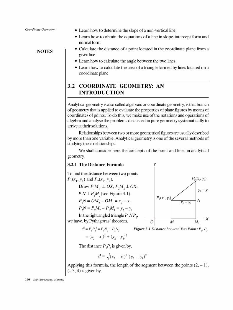
160 Self-Instructional Material
Coordinate Geometry
NOTES
• Learn how to determine the slope of a non-vertical line
• Learn how to obtain the equations of a line in slope-intercept form and
normal form
• Calculate the distance of a point located in the coordinate plane from a
given line
• Learn how to calculate the angle between the two lines
• Learn how to calculate the area of a triangle formed by lines located on a
coordinate plane
3.2 COORDINATE GEOMETRY: AN
INTRODUCTION
Analytical geometry is also called algebraic or coordinate geometry, is that branch
of geometry that is applied to evaluate the properties of plane figures by means of
coordinates of points. To do this, we make use of the notations and operations of
algebra and analyse the problems discussed in pure geometry systematically to
arrive at their solutions.
Relationships between two or more geometrical figures are usually described
by more than one variable. Analytical geometry is one of the several methods of
studying these relationships.
We shall consider here the concepts of the point and lines in analytical
geometry.
3.2.1 The Distance Formula
To find the distance between two points
P1(x
1, y
1) and P
2(x
2, y
2).
Draw P1M
1 ⊥ OX, P
2M
2 ⊥ OX,
P1N ⊥ P
2M
2 (see Figure 3.1)
Y
P x y( , )22 2
y y – 12
NP x y1 1 1( , )
x x – 12
O M1 M2
X
P1N = OM
2 – OM
1 = x
2 – x
1
P2N = P
2M
2 – P
1M
1 = y
2 – y
1
In the right angled triangle P1 N P
2,
we have, by Pythagoras’ theorem,
d2 = P1P
2
2 = P1N
2 + P
2N
2 Figure 3.1 Distance between Two Points P
1, P
2
= (x2 – x
1)2 + (y
2 – y
1)2
The distance P1P
2 is given by,
d = 2 2
2 1 2 1( – ) ( – )x x y y
Applying this formula, the length of the segment between the points (2, – 1),
(– 3, 4) is given by,
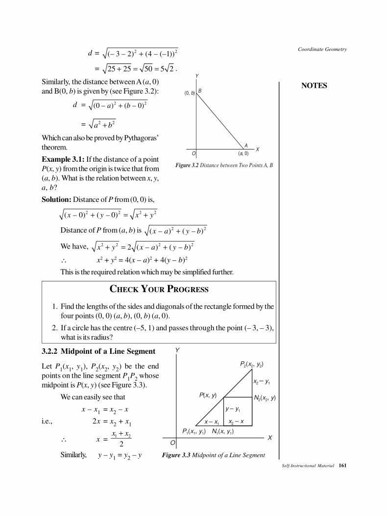
Coordinate Geometry
NOTES
Self-Instructional Material 161
d = 2 2(– 3 – 2) (4 – (–1))+
= 25 25 50 5 2+ = = .
Similarly, the distance between A (a, 0)
and B(0, b) is given by (see Figure 3.2):
Y
(0, )b
OX
( , 0)a
Figure 3.2 Distance between Two Points A, B
A
B
d = 2 2(0 – ) ( – 0)a b+
= 2 2a b+
Which can also be proved by Pythagoras’
theorem.
Example 3.1: If the distance of a point
P(x, y) from the origin is twice that from
(a, b). What is the relation between x, y,
a, b?
Solution: Distance of P from (0, 0) is,
2 2 2 2( – 0) ( – 0)x y x y+ = +
Distance of P from (a, b) is 2 2( – ) ( – )x a y b+
We have, 2 2 2 22 ( – ) ( – )x y x a y b+ = +
∴ x2 + y2 = 4(x – a)2 + 4(y – b)2
This is the required relation which may be simplified further.
CHECK YOUR PROGRESS
1. Find the lengths of the sides and diagonals of the rectangle formed by the
four points (0, 0) (a, b), (0, b) (a, 0).
2. If a circle has the centre (–5, 1) and passes through the point (– 3, – 3),
what is its radius?
3.2.2 Midpoint of a Line Segment
Let P1(x
1, y
1), P
2(x
2, y
2) be the end
points on the line segment P1P
2 whose
midpoint is P(x, y) (see Figure 3.3).
We can easily see that
Y
y y – 1
P x y1 1 1( , )
x x – 2
O
N x y1 1( , )
x x – 1
P x y( , ) N x y2 2( , )
x y2 1–
P x y2 2 2( , )
X
x – x1
= x2 – x
i.e., 2x = x2 + x
1
∴ x = 1 2
2
x x+
Similarly, y – y1
= y2 – y Figure 3.3 Midpoint of a Line Segment
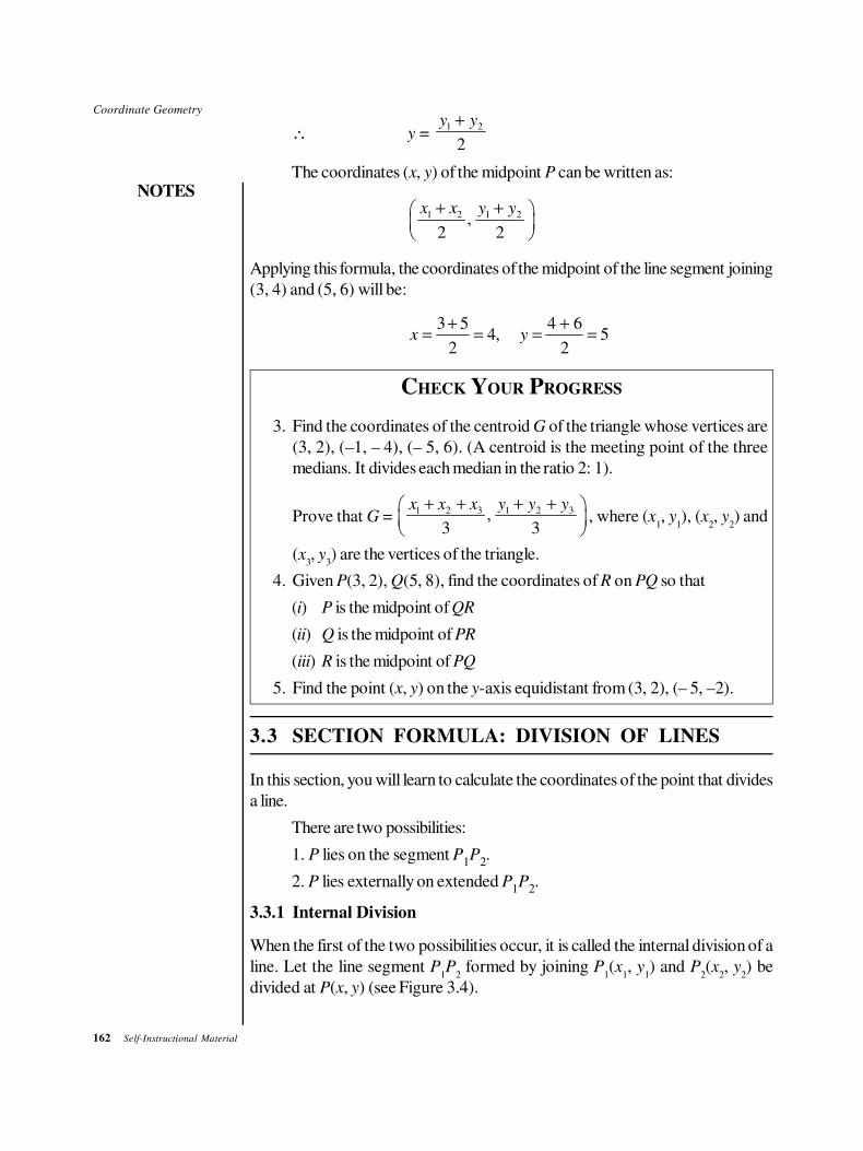
162 Self-Instructional Material
Coordinate Geometry
NOTES
∴ y = 1 2
2
y y+
The coordinates (x, y) of the midpoint P can be written as:
1 2 1 2,2 2
x x y y+ +
Applying this formula, the coordinates of the midpoint of the line segment joining
(3, 4) and (5, 6) will be:
3 5 4 64, 5
2 2x y
+ += = = =
CHECK YOUR PROGRESS
3. Find the coordinates of the centroid G of the triangle whose vertices are
(3, 2), (–1, – 4), (– 5, 6). (A centroid is the meeting point of the three
medians. It divides each median in the ratio 2: 1).
Prove that G = 1 2 3 1 2 3,
3 3
x x x y y y+ + + +
, where (x1, y
1), (x
2, y
2) and
(x3, y
3) are the vertices of the triangle.
4. Given P(3, 2), Q(5, 8), find the coordinates of R on PQ so that
(i) P is the midpoint of QR
(ii) Q is the midpoint of PR
(iii) R is the midpoint of PQ
5. Find the point (x, y) on the y-axis equidistant from (3, 2), (– 5, –2).
3.3 SECTION FORMULA: DIVISION OF LINES
In this section, you will learn to calculate the coordinates of the point that divides
a line.
There are two possibilities:
1. P lies on the segment P1P
2.
2. P lies externally on extended P1P
2.
3.3.1 Internal Division
When the first of the two possibilities occur, it is called the internal division of a
line. Let the line segment P1P
2 formed by joining P
1(x
1, y
1) and P
2(x
2, y
2) be
divided at P(x, y) (see Figure 3.4).
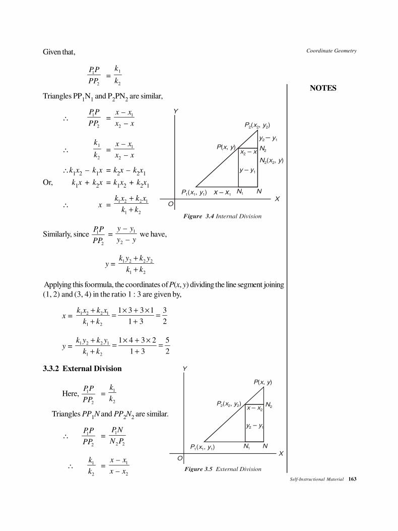
Coordinate Geometry
NOTES
Self-Instructional Material 163
Given that,
1
2
PP
PP=
1
2
k
k
Triangles PP1N
1 and P
2PN
2 are similar,
∴1
2
PP
PP=
1
2
–
–
x x
x x
∴1
2
k
k=
1
2
–
–
x x
x x
Y
y y – 1
P x y1 1 1( , )
x x – 2
O
x x – 1
P x y( , )
N x y2 2( , )
y y2 1–
P x y2 2 2( , )
X
N2
N1 N
Figure 3.4 Internal Division
∴k1x
2 – k
1x = k
2x – k
2x
1
Or, k1x + k
2x = k
1x
2 + k
2x
1
∴ x = 1 2 2 1
1 2
k x k x
k k
+
+
Similarly, since 1
2
PP
PP =
1
2
–
–
y y
y y we have,
y = 1 2 2 2
1 2
k y k y
k k
+
+
Applying this foormula, the coordinates of P(x, y) dividing the line segment joining
(1, 2) and (3, 4) in the ratio 1 : 3 are given by,
x = 1 2 2 1
1 2
1 3 3 1 3
1 3 2
k x k x
k k
+ × + ×= =
+ +
y = 1 2 2 1
1 2
1 4 3 2 5
1 3 2
k y k y
k k
+ × + ×= =
+ +
3.3.2 External Division
Here, 1
2
PP
PP=
1
2
k
k
Triangles PP1N and PP
2N
2 are similar.
Y
y y2 1 –
P x y1 1 1( , )
x x – 2
O
P x y( , )22 2
P x y( , )
X
N2
N1 N
Figure 3.5 External Division
∴ 1
2
PP
PP=
1
2 2
P N
N P
∴ 1
2
k
k=
1
2
–
–
x x
x x
164 Self-Instructional Material
Coordinate Geometry
NOTES
∴ k1(x – x
2) = k
2(x – x
1)
k1x – k
1x
2= k
2x – k
2x
1
∴ x(k1 – k
2) = k
1x
2 – k
2x
1
Thus, we have x = 1 2 2 1
1 2
–
–
k x k x
k k
Similarly, y = 1 2 2 1
1 2
–
–
k y k y
k k
Applying this formula, the coordinates of P(x, y) dividing the line segment joining
(1, 2) and (3, 4) externally in the ratio 5 : 4 are given by,
x = 5 3 – 4 1
115 – 4
× ×=
y = 5 4 – 4 2
125 – 4
× ×=
Hence, we learnt that:
• The coordinates of internal division are 1 2 2 1 1 2 2 1
1 2 1 2
,k x k x k y k y
k k k k
+ +
+ + .
• The coordinates of external division are
1 2 2 1 1 2 2 1
1 2 1 2
– –,
– –
k x k x k y k y
k k k k
or 2 1 1 2 2 1 1 2
2 1 2 1
– –,
– –
k x k x k y k y
k k k k
.
Example 3.2: In what ratio does the origin divide line joining (6, 0), (– 3, 0)?
Solution: Let the ratio be k : 1. Origin liss between these two points. Hence, it is
an internal division. Then two coordinates of the dividing point, i.e., (0, 0) are
x = (– 3) 1.6
0, 01
ky
k
+= =
+
∴ – 3k + 6 = 0 or k = 2 the ratio is 2 : 1
CHECK YOUR PROGRESS
6. If one end of the diameter of a circle with centre C(– 4, 1) is P(2, 6), find
the coordinates of the other end of the diameter.
7. Write the coordinates of the point of trisection of the line segment joining
(1, 0), (8, 10).
8. Find the ratio of which the Y-axis divides the join of (3, 5), (6, 7).
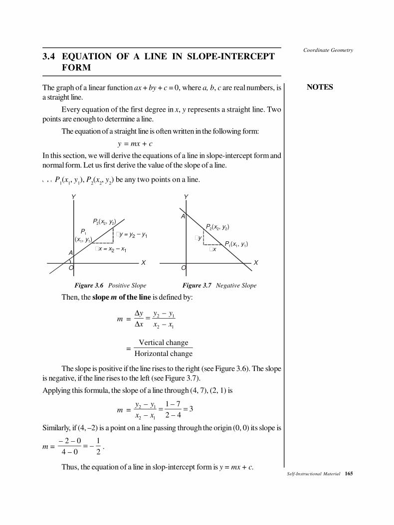
Coordinate Geometry
NOTES
Self-Instructional Material 165
3.4 EQUATION OF A LINE IN SLOPE-INTERCEPT
FORM
The graph of a linear function ax + by + c = 0, where a, b, c are real numbers, is
a straight line.
Every equation of the first degree in x, y represents a straight line. Two
points are enough to determine a line.
The equation of a straight line is often written in the following form:
y = mx + c
In this section, we will derive the equations of a line in slope-intercept form and
normal form. Let us first derive the value of the slope of a line.
L e t P1(x
1, y
1), P
2(x
2, y
2) be any two points on a line.
P
x y1
1 1( , )
P x y( , )22 2
A
OX
Y
P x y1 1 1( , )
P x y( , )22 2
A
OX
Y
�y = y – y2 1
�x = x – x2 1 �x
�y
Figure 3.6 Positive Slope Figure 3.7 Negative Slope
Then, the slope m of the line is defined by:
m = 2 1
2 1
–
–
y y y
x x x
∆=
∆
= Vertical change
Horizontal change
The slope is positive if the line rises to the right (see Figure 3.6). The slope
is negative, if the line rises to the left (see Figure 3.7).
Applying this formula, the slope of a line through (4, 7), (2, 1) is
m = 2 1
2 1
– 1 – 73
– 2 – 4
y y
x x= =
Similarly, if (4, –2) is a point on a line passing through the origin (0, 0) its slope is
m = – 2 – 0 1
–4 – 0 2
= .
Thus, the equation of a line in slop-intercept form is y = mx + c.
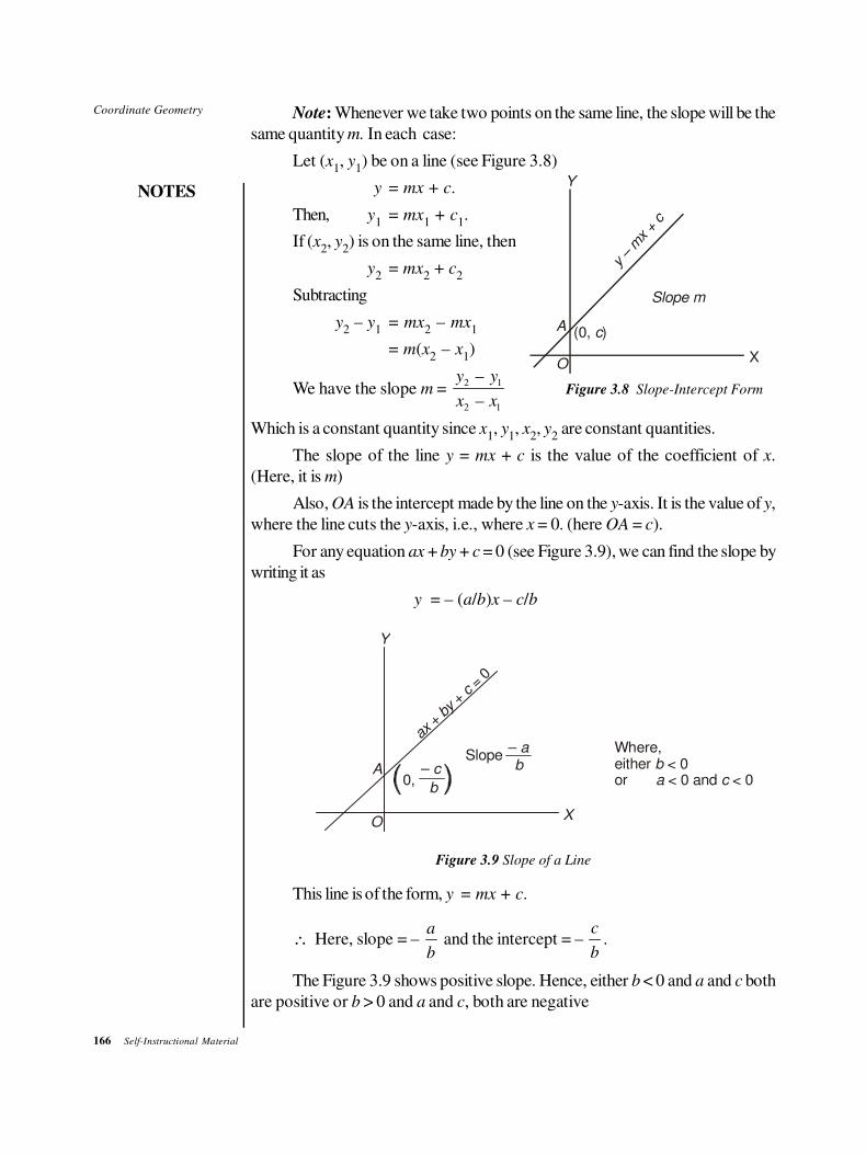
166 Self-Instructional Material
Coordinate Geometry
NOTES
Note: Whenever we take two points on the same line, the slope will be the
same quantity m. In each case:
Let (x1, y
1) be on a line (see Figure 3.8)
y = mx + c.
Then, y1
= mx1 + c
1.
If (x2, y
2) is on the same line, then
y2
= mx2 + c
2
Y
X
y –
mx +
c
A
O
(0, )c
Slope mSubtracting
y2 – y
1= mx
2 – mx
1
= m(x2 – x
1)
We have the slope m = 2 1
2 1
–
–
y y
x xFigure 3.8 Slope-Intercept Form
Which is a constant quantity since x1, y
1, x
2, y
2 are constant quantities.
The slope of the line y = mx + c is the value of the coefficient of x.
(Here, it is m)
Also, OA is the intercept made by the line on the y-axis. It is the value of y,
where the line cuts the y-axis, i.e., where x = 0. (here OA = c).
For any equation ax + by + c = 0 (see Figure 3.9), we can find the slope by
writing it as
y = – (a/b)x – c/b
Y
X
axby
c
+
+
= 0
A
O
Slope– ab
0,– c
b
Where, either < 0or < 0 and < 0
ba c
Figure 3.9 Slope of a Line
This line is of the form, y = mx + c.
∴ Here, slope = – a
b and the intercept = –
c
b.
The Figure 3.9 shows positive slope. Hence, either b < 0 and a and c both
are positive or b > 0 and a and c, both are negative
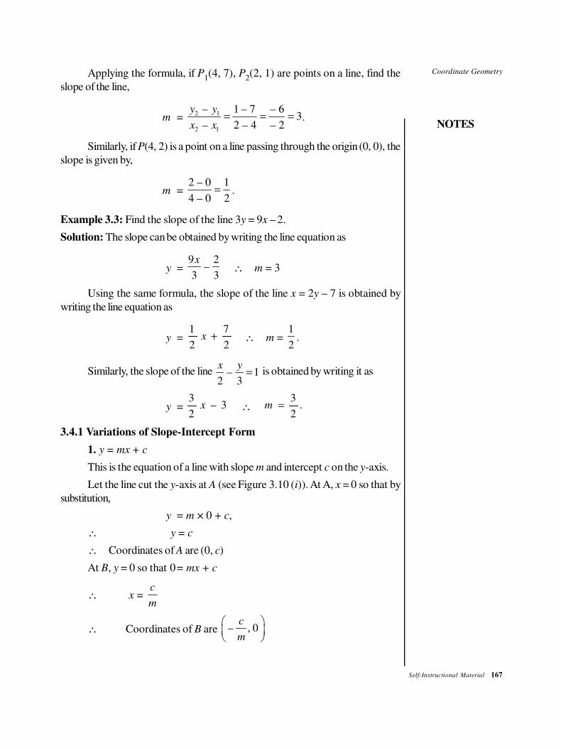
Coordinate Geometry
NOTES
Self-Instructional Material 167
Applying the formula, if P1(4, 7), P
2(2, 1) are points on a line, find the
slope of the line,
m = 2 1
2 1
– 1 – 7 – 63
– 2 – 4 – 2
y y
x x= = = .
Similarly, if P(4, 2) is a point on a line passing through the origin (0, 0), the
slope is given by,
m = 2 – 0 1
4 – 0 2= .
Example 3.3: Find the slope of the line 3y = 9x – 2.
Solution: The slope can be obtained by writing the line equation as
y = 9 2
–3 3
x∴ m = 3
Using the same formula, the slope of the line x = 2y – 7 is obtained by
writing the line equation as
y = 1 7
2 2x + ∴ m =
1–
2.
Similarly, the slope of the line – 12 3
x y= is obtained by writing it as
y = 3
– 32
x ∴3
.2
m =
3.4.1 Variations of Slope-Intercept Form
1. y = mx + c
This is the equation of a line with slope m and intercept c on the y-axis.
Let the line cut the y-axis at A (see Figure 3.10 (i)). At A, x = 0 so that by
substitution,
y = m × 0 + c,
∴ y = c
∴ Coordinates of A are (0, c)
At B, y = 0 so that 0= mx + c
∴ x = c
m
∴ Coordinates of B are – , 0c
m
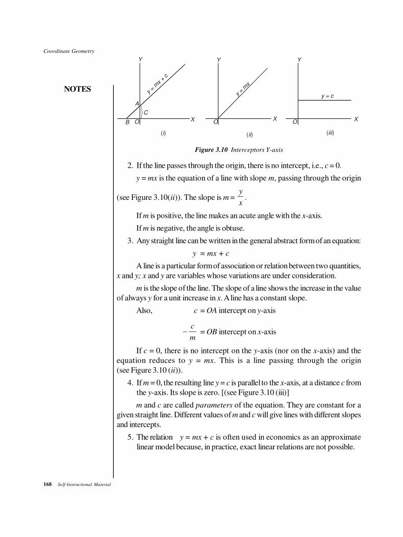
168 Self-Instructional Material
Coordinate Geometry
NOTES
Y
X
y =
mx + c
A
OB
Y
X
y =
mx
O
Y
XO
y = c
( )iii( )ii( )i
C
Figure 3.10 Interceptors Y-axis
2. If the line passes through the origin, there is no intercept, i.e., c = 0.
y = mx is the equation of a line with slope m, passing through the origin
(see Figure 3.10(ii)). The slope is m = y
x.
If m is positive, the line makes an acute angle with the x-axis.
If m is negative, the angle is obtuse.
3. Any straight line can be written in the general abstract form of an equation:
y = mx + c
A line is a particular form of association or relation between two quantities,
x and y; x and y are variables whose variations are under consideration.
m is the slope of the line. The slope of a line shows the increase in the value
of always y for a unit increase in x. A line has a constant slope.
Also, c = OA intercept on y-axis
–c
m= OB intercept on x-axis
If c = 0, there is no intercept on the y-axis (nor on the x-axis) and the
equation reduces to y = mx. This is a line passing through the origin
(see Figure 3.10 (ii)).
4. If m = 0, the resulting line y = c is parallel to the x-axis, at a distance c from
the y-axis. Its slope is zero. [(see Figure 3.10 (iii)]
m and c are called parameters of the equation. They are constant for a
given straight line. Different values of m and c will give lines with different slopes
and intercepts.
5. The relation y = mx + c is often used in economics as an approximate
linear model because, in practice, exact linear relations are not possible.
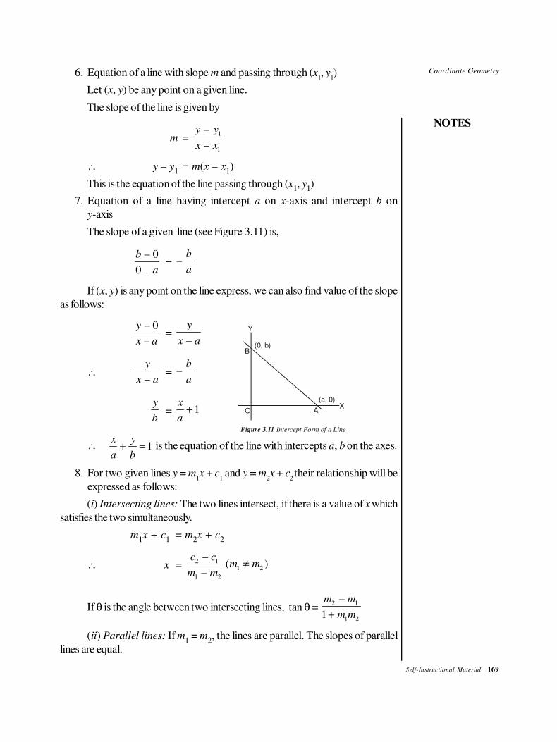
Coordinate Geometry
NOTES
Self-Instructional Material 169
6. Equation of a line with slope m and passing through (x1, y
1)
Let (x, y) be any point on a given line.
The slope of the line is given by
m = 1
1
–
–
y y
x x
∴ y – y1
= m(x – x1)
This is the equation of the line passing through (x1, y
1)
7. Equation of a line having intercept a on x-axis and intercept b on
y-axis
The slope of a given line (see Figure 3.11) is,
– 0
0 –
b
a= –
b
a
If (x, y) is any point on the line express, we can also find value of the slope
as follows:
– 0
–
y
x a=
–
y
x a
B
OX
Y
A
(a, 0)
(0, b)
Figure 3.11 Intercept Form of a Line
∴–
y
x a= –
b
a
y
b= 1
x
a+
∴ 1x y
a b+ = is the equation of the line with intercepts a, b on the axes.
8. For two given lines y = m1x + c
1 and y = m
2x + c
2 their relationship will be
expressed as follows:
(i) Intersecting lines: The two lines intersect, if there is a value of x which
satisfies the two simultaneously.
m1x + c
1= m
2x + c
2
∴ x = 2 1
1 2
1 2
–( )
–
c cm m
m m≠
If θ is the angle between two intersecting lines, tan θ = 2 1
1 2
–
1
m m
m m+
(ii) Parallel lines: If m1 = m
2, the lines are parallel. The slopes of parallel
lines are equal.
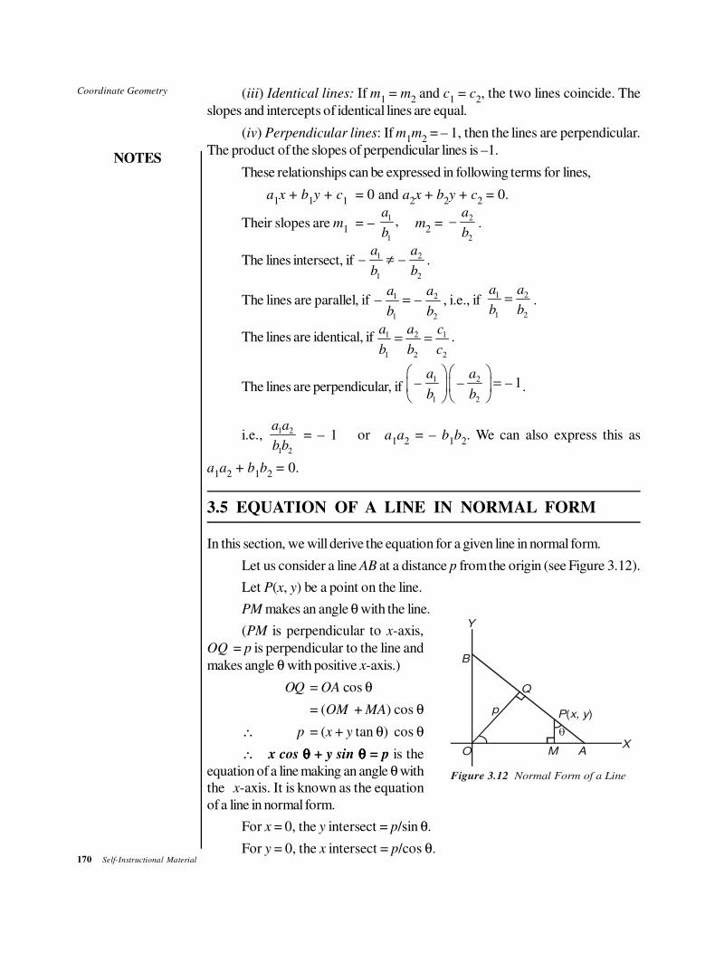
170 Self-Instructional Material
Coordinate Geometry
NOTES
(iii) Identical lines: If m1 = m
2 and c
1 = c
2, the two lines coincide. The
slopes and intercepts of identical lines are equal.
(iv) Perpendicular lines: If m1m
2 = – 1, then the lines are perpendicular.
The product of the slopes of perpendicular lines is –1.
These relationships can be expressed in following terms for lines,
a1x + b
1y + c
1= 0 and a
2x + b
2y + c
2 = 0.
Their slopes are m1
= – 1
1
,a
bm
2 =
2
2
–a
b.
The lines intersect, if 1 2
1 2
– –a a
b b≠ .
The lines are parallel, if 1 2
1 2
– –a a
b b= , i.e., if
1 2
1 2
a a
b b= .
The lines are identical, if 1 2 1
1 2 2
a a c
b b c= = .
The lines are perpendicular, if 1 2
1 2
– – – 1a a
b b
=
.
i.e., 1 2
1 2
a a
b b = – 1 or a
1a
2 = – b
1b
2. We can also express this as
a1a
2 + b
1b
2 = 0.
3.5 EQUATION OF A LINE IN NORMAL FORM
In this section, we will derive the equation for a given line in normal form.
Let us consider a line AB at a distance p from the origin (see Figure 3.12).
Let P(x, y) be a point on the line.
PM makes an angle θ with the line.
(PM is perpendicular to x-axis,
OQ = p is perpendicular to the line and
makes angle θ with positive x-axis.)
OQ = OA cos θ
B
OX
Y
A
P x, y( )
M
Q
p
Figure 3.12 Normal Form of a Line
= (OM + MA) cos θ
∴ p = (x + y tan θ) cos θ
∴ x cos θθθθ + y sin θθθθ = p is the
equation of a line making an angle θ with
the x-axis. It is known as the equation
of a line in normal form.
For x = 0, the y intersect = p/sin θ.
For y = 0, the x intersect = p/cos θ.
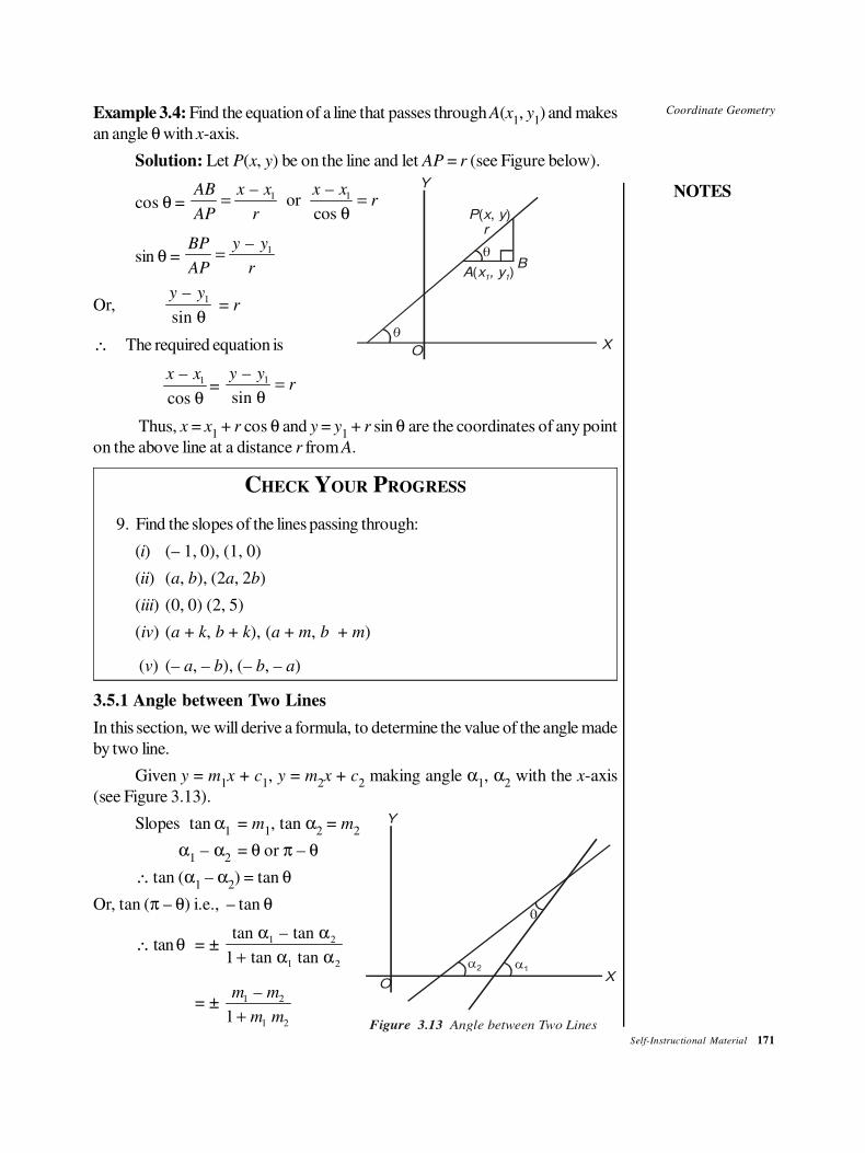
Coordinate Geometry
NOTES
Self-Instructional Material 171
Example 3.4: Find the equation of a line that passes through A(x1, y
1) and makes
an angle θ with x-axis.
Solution: Let P(x, y) be on the line and let AP = r (see Figure below).
cos θ = 1 1– –
orcos
AB x x x xr
AP r= =
θ
sin θ = 1–BP y y
AP r=
Or, 1–
sin
y y
θ = r
Y
X
A x , y( )11
O
B
rP x y( , )
Figure 3.13
∴ The required equation is
1–
cos
x x
θ=
1–
sin
y yr=
θ
Thus, x = x1 + r cos θ and y = y
1 + r sin θ are the coordinates of any point
on the above line at a distance r from A.
CHECK YOUR PROGRESS
9. Find the slopes of the lines passing through:
(i) (– 1, 0), (1, 0)
(ii) (a, b), (2a, 2b)
(iii) (0, 0) (2, 5)
(iv) (a + k, b + k), (a + m, b + m)
(v) (– a, – b), (– b, – a)
3.5.1 Angle between Two Lines
In this section, we will derive a formula, to determine the value of the angle made
by two line.
Given y = m1x + c
1, y = m
2x + c
2 making angle α
1, α
2 with the x-axis
(see Figure 3.13).
Slopes tan α1
= m1, tan α
2 = m
2
α1 – α
2= θ or π – θ
∴ tan (α1 – α
2) = tan θ
Or, tan (π – θ) i.e., – tan θ
Y
XO
Figure 3.13 Angle between Two Lines
∴ tan θ = ± 1 2
1 2
tan – tan
1 tan tan
α α
+ α α
= ± 1 2
1 2
–
1
m m
m m+
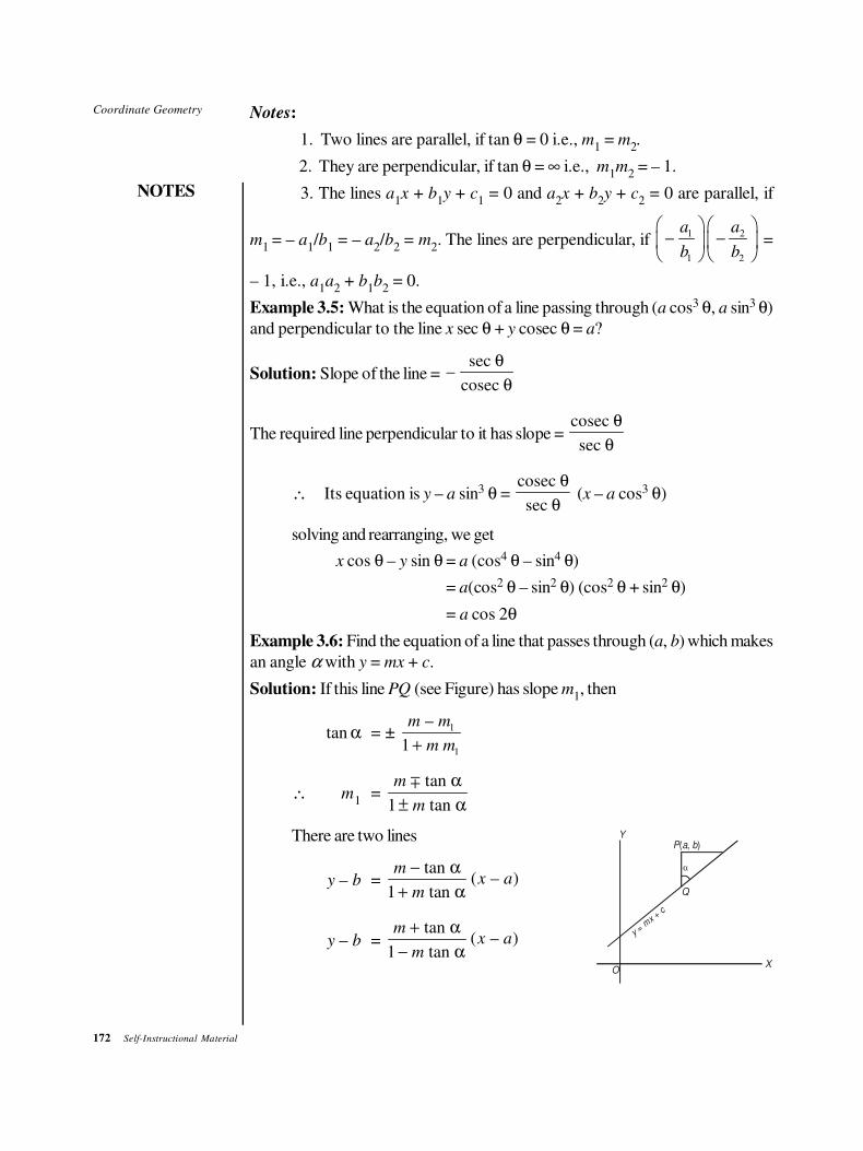
172 Self-Instructional Material
Coordinate Geometry
NOTES
Notes:
1. Two lines are parallel, if tan θ = 0 i.e., m1 = m
2.
2. They are perpendicular, if tan θ = ∞ i.e., m1m
2 = – 1.
3. The lines a1x + b
1y + c
1 = 0 and a
2x + b
2y + c
2 = 0 are parallel, if
m1
= – a1/b
1 = – a
2/b
2 = m
2. The lines are perpendicular, if
1 2
1 2
– –a a
b b
=
– 1, i.e., a1a
2 + b
1b
2 = 0.
Example 3.5: What is the equation of a line passing through (a cos3 θ, a sin3 θ)
and perpendicular to the line x sec θ + y cosec θ = a?
Solution: Slope of the line = sec
–cosec
θ
θ
The required line perpendicular to it has slope = cosec
sec
θ
θ
∴ Its equation is y – a sin3 θ = cosec
sec
θ
θ (x – a cos3 θ)
solving and rearranging, we get
x cos θ – y sin θ = a (cos4 θ – sin4 θ)
= a(cos2 θ – sin2 θ) (cos2 θ + sin2 θ)
= a cos 2θ
Example 3.6: Find the equation of a line that passes through (a, b) which makes
an angle α with y = mx + c.
Solution: If this line PQ (see Figure) has slope m1, then
tan α = ± 1
1
–
1
m m
m m+
∴ m1
= tan
1 tan
m
m
α
± α
∓
There are two lines
OX
Q
P a b( , )Y
ym
xc
=
+
y – b = tan
( – )1 tan
mx a
m
− α
+ α
y – b = tan
( – )1 tan
mx a
m
+ α
− α
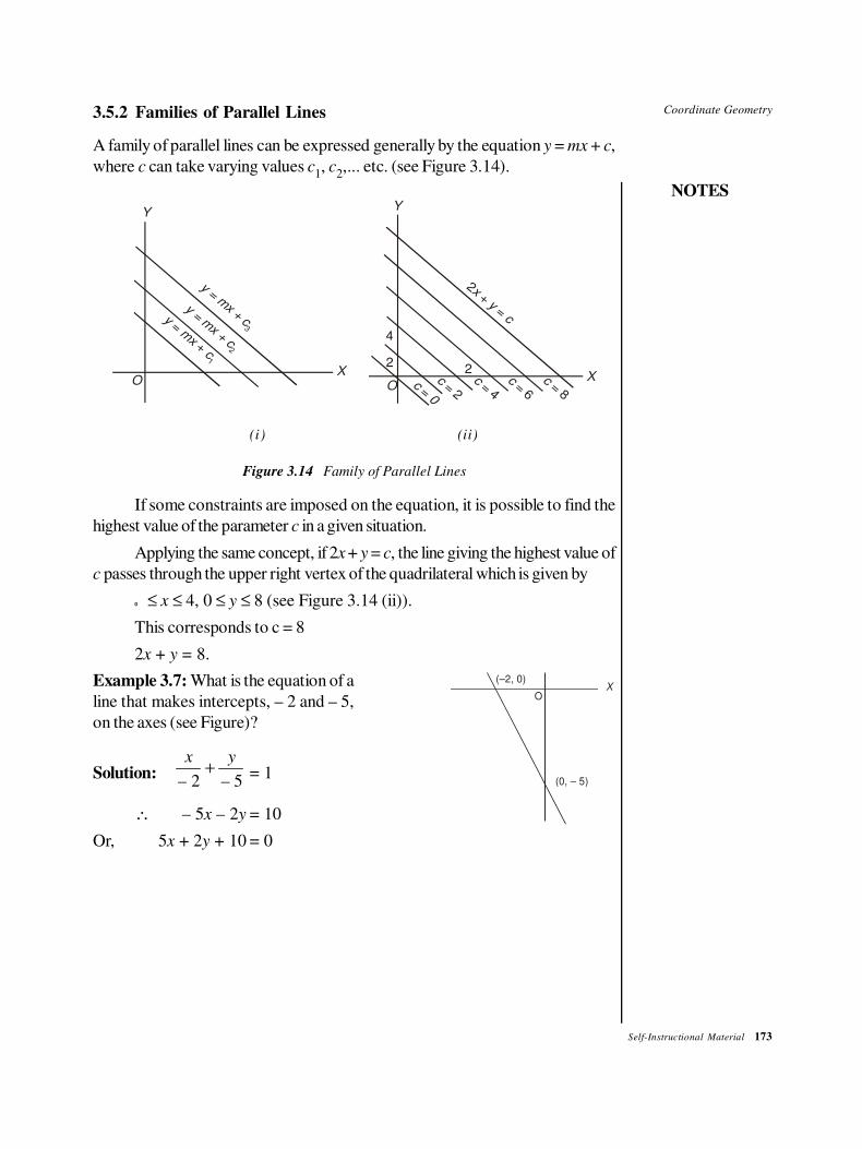
Coordinate Geometry
NOTES
Self-Instructional Material 173
3.5.2 Families of Parallel Lines
A family of parallel lines can be expressed generally by the equation y = mx + c,
where c can take varying values c1, c
2,... etc. (see Figure 3.14).
OX
Y
OX
Y
2
4
2c = 2
c = 4c = 6
c = 8
2 +
=
xy
c
y = mx + c
3
y = mx + c
2
ym
xc
= +
1
c0
=
(i) (ii)
Figure 3.14 Family of Parallel Lines
If some constraints are imposed on the equation, it is possible to find the
highest value of the parameter c in a given situation.
Applying the same concept, if 2x + y = c, the line giving the highest value of
c passes through the upper right vertex of the quadrilateral which is given by
0 ≤ x ≤ 4, 0 ≤ y ≤ 8 (see Figure 3.14 (ii)).
This corresponds to c = 8
2x + y = 8.
Example 3.7: What is the equation of a
line that makes intercepts, – 2 and – 5,
on the axes (see Figure)?
Solution:– 2 – 5
x y+ = 1
XO
(0, – 5)
(–2, 0)
∴ – 5x – 2y = 10
Or, 5x + 2y + 10 = 0
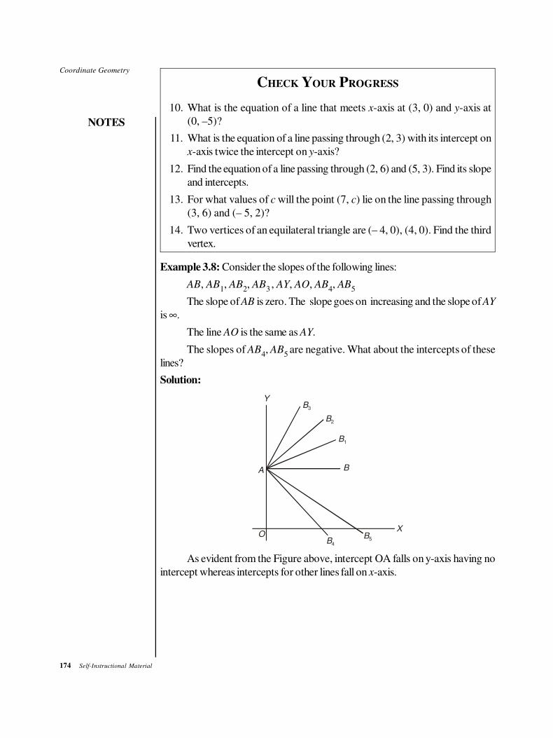
174 Self-Instructional Material
Coordinate Geometry
NOTES
CHECK YOUR PROGRESS
10. What is the equation of a line that meets x-axis at (3, 0) and y-axis at
(0, –5)?
11. What is the equation of a line passing through (2, 3) with its intercept on
x-axis twice the intercept on y-axis?
12. Find the equation of a line passing through (2, 6) and (5, 3). Find its slope
and intercepts.
13. For what values of c will the point (7, c) lie on the line passing through
(3, 6) and (– 5, 2)?
14. Two vertices of an equilateral triangle are (– 4, 0), (4, 0). Find the third
vertex.
Example 3.8: Consider the slopes of the following lines:
AB, AB1, AB
2, AB
3 , AY, AO, AB
4, AB
5
The slope of AB is zero. The slope goes on increasing and the slope of AY
is ∞.
The line AO is the same as AY.
The slopes of AB4, AB
5 are negative. What about the intercepts of these
lines?
Solution:
OB4
B5
X
B
B1
B2
B3
Y
A
As evident from the Figure above, intercept OA falls on y-axis having no
intercept whereas intercepts for other lines fall on x-axis.
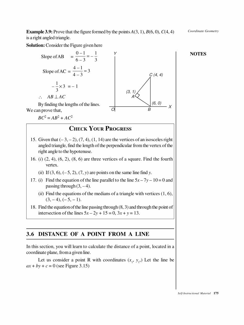
Coordinate Geometry
NOTES
Self-Instructional Material 175
Example 3.9: Prove that the figure formed by the points A(3, 1), B(6, 0), C(4, 4)
is a right angled triangle.
Solution: Consider the Figure given here
Slope of AB = 0 – 1 1
–6 – 3 3
=
Slope of AC = 4 – 1
34 – 3
=
1– 3
3× = – 1
OX
Y
B
A
C (4, 4)
(3, 1)
(6, 0)
∴ AB ⊥ AC
By finding the lengths of the lines.
We can prove that,
BC2 = AB2 + AC2
CHECK YOUR PROGRESS
15. Given that (– 3, – 2), (7, 4), (1, 14) are the vertices of an isosceles right
angled triangle, find the length of the perpendicular from the vertex of the
right angle to the hypotenuse.
16. (i) (2, 4), (6, 2), (8, 6) are three vertices of a square. Find the fourth
vertex.
(ii) If (3, 6), (– 5, 2), (7, y) are points on the same line find y.
17. (i) Find the equation of the line parallel to the line 5x – 7y – 10 = 0 and
passing through (3, – 4).
(ii) Find the equations of the medians of a triangle with vertices (1, 6),
(3, – 4), (– 5, – 1).
18. Find the equation of the line passing through (8, 3) and through the point of
intersection of the lines 5x – 2y + 15 = 0, 3x + y = 13.
3.6 DISTANCE OF A POINT FROM A LINE
In this section, you will learn to calculate the distance of a point, located in a
coordinate plane, from a given line.
Let us consider a point R with coordinates (x1, y
1,) Let the line be
ax + by + c = 0 (see Figure 3.15)
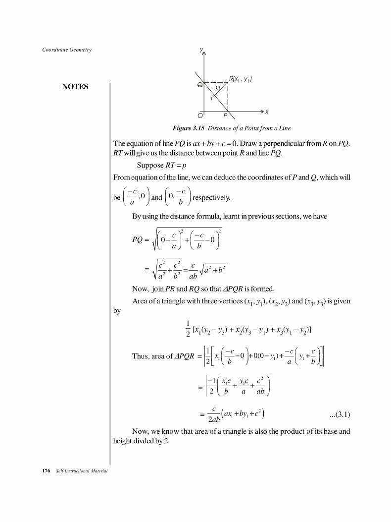
176 Self-Instructional Material
Coordinate Geometry
NOTES
y
x
Q p
R(x , y )1 1
T
O P
Figure 3.15 Distance of a Point from a Line
The equation of line PQ is ax + by + c = 0. Draw a perpendicular from R on PQ.
RT will give us the distance between point R and line PQ.
Suppose RT = p
From equation of the line, we can deduce the coordinates of P and Q, which will
be ,0c
a
−
and 0,c
b
−
respectively..
By using the distance formula, learnt in previous sections, we have
PQ =
2 2
0 0c c
a b
− + + −
= 2 2
2 2
2 2
c c ca b
a b ab+ = +
Now, join PR and RQ so that ∆PQR is formed.
Area of a triangle with three vertices (x1, y
1), (x
2, y
2) and (x
3, y
3) is given
by
1
2[x
1(y
2 – y
3) + x
2(y
3 – y
1) + x
3(y
1 – y
2)]
Thus, area of ∆PQR = 1 1 1
10 0(0 )
2
c c cx y y
b a b
− − − + − + +
=
2
1 11
2
x c y c c
b a ab
−+ +
= ( )2
1 12
cax by c
ab+ + ...(3.1)
Now, we know that area of a triangle is also the product of its base and
height divded by 2.
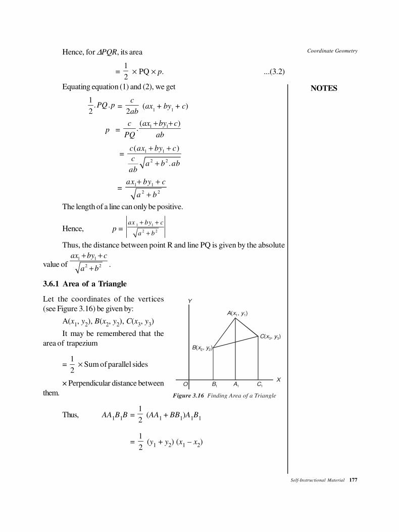
Coordinate Geometry
NOTES
Self-Instructional Material 177
Hence, for ∆PQR, its area
= 1
2 × PQ × p. ...(3.2)
Equating equation (1) and (2), we get
1
. .2
PQ p = 2
c
ab (ax
1 + by
1 + c)
p = 1 1( )
.c ax by c
PQ ab
+ +
= 1 1
2 2
( )
.
c ax by c
ca b ab
ab
+ +
+
= 1 1
2 2
ax by c
a b
+ +
+
The length of a line can only be positive.
Hence, p = 1 1
2 2
ax by c
a b
+ +
+
Thus, the distance between point R and line PQ is given by the absolute
value of 1 1
2 2
ax by c
a b
+ +
+.
3.6.1 Area of a Triangle
Let the coordinates of the vertices
(see Figure 3.16) be given by:
A(x1, y
2), B(x
2, y
2), C(x
3, y
3)
Y
OX
A x y( , )1 1
C x y( , )3 3
B x y( , )2 2
C1A1B1
Figure 3.16 Finding Area of a Triangle
It may be remembered that the
area of trapezium
= 1
2 × Sum of parallel sides
× Perpendicular distance between
them.
Thus, AA1B
1B =
1
2 (AA
1 + BB
1)A
1B
1
= 1
2 (y
1 + y
2) (x
1 – x
2)
178 Self-Instructional Material
Coordinate Geometry
NOTES
∆ABC = Trap. AA1B
1B + Trap. ACC
1A
1 – Trap. BCC
1B
1
= 1
2(y
1 + y
2) (x
1 – x
2) +
1
2 (y
1 + y
3) (x
3 – x
1)
– 1
2 (y
2 + y
3) (x
3 – x
2)
= 1
2(x
1y
2 – x
2y
1 + x
2y
3 – x
3y
2 + x
3y
1 – x
1y
3)
= 1
2[(x
1 (y
2 – y
3) + x
2 (y
3 – y
1) + x
3 (y
1 – y
2)
If three points lie on a straight line, the area of the triangle formed by themis zero, i.e., = 0. Infact, this is the condition for three points to be on a line
(collinearity). = 1
2[(x
1 (y
2 – y
3) + x
2 (y
3 – y
1) + x
3 (y
1 – y
2)
CHECK YOUR PROGRESS
19. Find the area of a triangle with vertices:
(i) (10, 7), (– 2, 3), (0, 0);
(ii) 91, 3) (5, 6), (2, 4)
20. If (0, 4), (– 1, 3), (k, 5) are collinear, find k.
3.7 SUMMARY
In this unit, you have learned that:
• ax + by + c = 0 is a linear equation. It is of degree one in x and y. It can be
represented geometrically by a straight line.
• If (x1, y
1), (x
2, y
2) are points on a line, its slope is defined by:
tan θ = m = 2 1
2 1
–
–
y y
x x
where θ is the smallest positive angle between the lines and the positive
x-axis. The rate of change of a linear function ax + by + c = 0 is constant
and equals the slope of the line.
• There are many forms of the equation of a straight line such as:
The slope-intercept from y = mx + c
The point-slope form y – y1 = m(x – x
1)
The two-point form 1
2 1
–
–
y y
y y =
1
2 1
–
–
x x
x x
The intercept form x y
a b+ = 1
Coordinate Geometry
NOTES
Self-Instructional Material 179
The line parallel to y-axis x = k
The line parallel to x-axis y = k
• In the general form ax + by + c = 0, the slope –a
mb
= and the intercepts
are –c
a
on x-axis and –c
b on y-axis.
If a = 0, the line is parallel to x-axis;
if b = 0, the line is parallel to y-axis.
• If two lines with slopes m1, m
2 are parallel, then m
1 = m
2 .
If they are perpendicular m1m
2 = – 1
• If θ is the angle between two perpendicular lines, then tan θ = 2 1
1 2
–
1
m m
m m+
• The coordinates of the point of intersection for two intersecting lines, obtained
by solving the equations, satisfy the equations of both the lines.
• Three given lines have a common point of intersection if the coordinates of
the intersection point on any two lines satisfy the equation of the third line.
• The normal form of the equation of a line is given by:
x cos θ + y sin θ = p
• The perpendicular distance of a given points (x1, y
1) from a given line
ax + by + c = 0 is given by:
p = 1 1
2 2
ax by c
a b
+ +
+
The perpendicular from the origin to this line is p = 2 2
c
a b+
• Distance between parallel lines is the perpendicular distance of any point on
one of the lines from the other line.
• Any line through the intersection of two given lines,
a1x + b
1y + c
1 = 0 and a
2x + b
2y + c
2 = 0 is expressed by:
a1x + b
1y + c
1 + k(a
2x + b
2y + c
2) = 0
Which represents the family of all lines passing through the point of intersection
of the given lines.
180 Self-Instructional Material
Coordinate Geometry
NOTES
3.8 KEY TERMS
•••• Coordinate geometry: It is the branch of mathematics that deals with the
evaluation of properties of plane figures by means of their location, in terms
of their coordinates, on a coordinate plane.
•••• External division of a line: When the point dividing a particular line falls
on the line only when it is extended, it is said to be an external division of
that line.
•••• Intercept: It is the distance between the origin and the points at which a
particular line intersects the two axes.
3.9 ANSWERS TO ‘CHECK YOUR PROGRESS’
1. a, b, a, b; 2 2 2 2,a b a b+ +
2. 17
3. (– 1, 4/3)
4. (i) (1, – 4)
(ii) (7, 14)
(iii) (4, 5)
5. (0, – 2)
6. (– 10 – 4)
7.13 14 17 22
, , ,3 3 3 3
8. External division – 1: 2
9. (i) 0
(ii) b/a
(iii) 5/2
(iv) 1
(v) –1
10. 13 – 5
x y+ = or – 1
3 5
x y= or 5x – 3y = 15
11. x + 2y – 8 = 0
12. x + y = 8; – 1; 8, 8
13. 8
Coordinate Geometry
NOTES
Self-Instructional Material 181
14. (0, 4 3)±
15. 2 17
16. (i) (4, 8)
(ii) The slopes of the lines joining any two of these three points will have the
same value of that y = 8
17. (i) 17x – 14y + 7 = 10,
(ii) 13x + 10y + 1 = 0, 2x – 7y + 3 = 0
18. x + y = 11
19. (i) 22
(ii) 1
2
20. 1
3.10 QUESTIONS AND EXERCISES
Short-Answer Questions
1. Find the third vertex if two vertices of an equilateral triangle are given to be
(0, 0), (– 4, 3).
2. Find the midpoint of (– a, 0), (4, 0).
3. Prove that A(0, 0), B(10, – 4) C(2, 5) form a right angled triangle.
4. The intercepts of parallel lines are different but the slopes are the same. Can
lines with negative and positive intercepts on the same axis be parallel?
5. Show that (0, 0), (a, 0), 2 2 2 2( – , ), ( – , )a a b b a b b+ are vertices of a
rhombus (a > b). Show that the diagonals are perpendicular.
6. Show that y = 7x + 2, 1
47
y x= + are perpendicular lines.
Hint. 1 2
17 – 1
2m m = × =
7. Show that (3, – 2), (4, 3), (– 1, 1), (– 2, – 4) are the vertices of a parallelogram.
Find the lengths of the diagonals.
(Hint: Find the slopes of opposite pairs of sides and show they are parallel
and equal.)
8. Show that the lines 3x + by + 5 = 0, cx – 3y – 2 = 0 are perpendicular, if
3c – 3b = 0 or b = c.
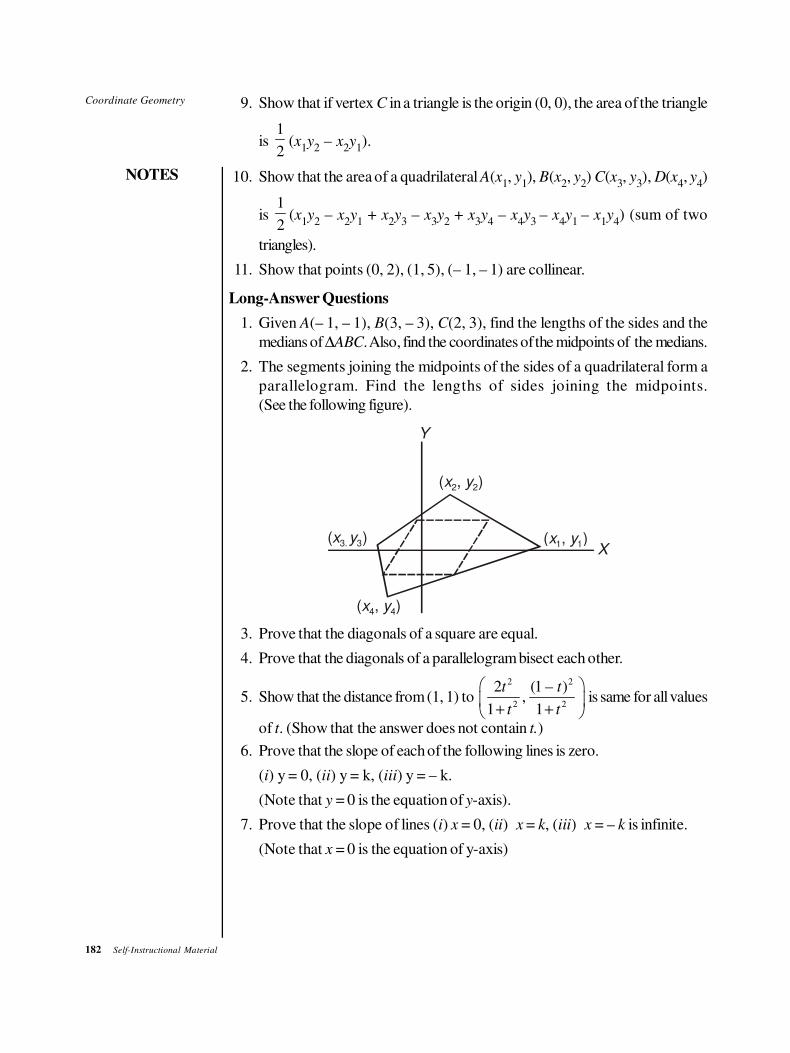
182 Self-Instructional Material
Coordinate Geometry
NOTES
9. Show that if vertex C in a triangle is the origin (0, 0), the area of the triangle
is 1
2(x
1y
2 – x
2y
1).
10. Show that the area of a quadrilateral A(x1, y
1), B(x
2, y
2) C(x
3, y
3), D(x
4, y
4)
is 1
2(x
1y
2 – x
2y
1 + x
2y
3 – x
3y
2 + x
3y
4 – x
4y
3 – x
4y
1 – x
1y
4) (sum of two
triangles).
11. Show that points (0, 2), (1, 5), (– 1, – 1) are collinear.
Long-Answer Questions
1. Given A(– 1, – 1), B(3, – 3), C(2, 3), find the lengths of the sides and the
medians of ∆ABC. Also, find the coordinates of the midpoints of the medians.
2. The segments joining the midpoints of the sides of a quadrilateral form a
parallelogram. Find the lengths of sides joining the midpoints.
(See the following figure).
( , )x y1 1
( , )x y22
( )x y3 3,
( , )x y4 4
X
Y
3. Prove that the diagonals of a square are equal.
4. Prove that the diagonals of a parallelogram bisect each other.
5. Show that the distance from (1, 1) to 2 2
2 2
2 (1 – ),
1 1
t t
t t
+ + is same for all values
of t. (Show that the answer does not contain t.)
6. Prove that the slope of each of the following lines is zero.
(i) y = 0, (ii) y = k, (iii) y = – k.
(Note that y = 0 is the equation of y-axis).
7. Prove that the slope of lines (i) x = 0, (ii) x = k, (iii) x = – k is infinite.
(Note that x = 0 is the equation of y-axis)
Coordinate Geometry
NOTES
Self-Instructional Material 183
8. Find the slopes of the following lines:
(i) 2 1
– 43 2
xy
+= (ii) – 3 6x y =
(iii) 3 12x y+ = (iv) y – 12x = 0
(v) x = y (vi) 2 6y x=
Are there any parallel or perpendicular lines among these?
Draw the graphs and check.
9. Prove that the following pairs of lines are parallel:
(i) y = 3x + 7 (ii) y = 7x (iii) y = x
y = 3x – 5 y = 1
72
x + y = x + a
(iv) ax + by + c = 0 (v) x = k (vi) y = 5
bx + k =
2b
ya
x = 0 y = – 5.
10. Prove that the following pairs of lines are perpendicular:
(i) y = 3x + 7 (ii) y = 2x (iii) 1x y
a b+ =
x = 5 – 3y3
–4 2
xy = ax – by = 10
(iv) ax + by + c = 0 (v) y = x
ay = bx x = – y.
11. (i) Prove that the lines joining the midpoints of opposite sides of a quadrilateral
bisect each other.
(ii) Prove that the diagonals of a rhombus are perpendicular.
12. Show that 1 2
1 2, , ,c ax c ax
x xb b
+ +
are points on the line ax + by = 0.
(Substitute each point in the equation and see if it is satisfied).
3.11 FURTHER READING
Khanna, V.K, S.K. Bhambri, C.B. Gupta and Vijay Gupta. Quantitative
Techniques. New Delhi: Vikas Publishing House.
Khanna, V.K, S.K. Bhambri and Quazi Zameeruddin. Business Mathematics.
New Delhi:Vikas Publishing House.

Quadratic Equations
NOTES
Self-Instructional Material 185
UNIT 4 QUADRATIC EQUATIONS
Structure
4.0 Introduction
4.1 Unit Objectives
4.2 Quadratric Equation: Basics4.2.1 Method of Solving Pure Quadratic Equations
4.3 Solving Quadratic Equations4.3.1 Method of Factorization
4.3.2 Method of Perfect Square
4.4 Discriminant Method and Nature of Roots
4.5 Relation of the Roots4.5.1 Symmetric Expression of Roots of a Quadratic Equation
4.5.2 Simultaneous Equations in Two Unknowns
4.5.3 Simultaneous Equations in Three or More than Three Unknowns
4.6 Summary
4.7 Key Terms
4.8 Answers to ‘Check Your Progress’
4.9 Questions and Exercises
4.10 Further Reading
4.0 INTRODUCTION
In mathematics, a quadratic equation is a polynomial equation of the second degree.
The general form is
Ax2 +bx+c=0
where x represents a variable, and a, b, and c, constants, with a ≠ 0.
(If a = 0, the equation is a linear equation.)The three constants—a, b and c— are
called the quadratic coefficient, the linear coefficient and the constant term or free
term, respectively. The term ‘quadratic’ is derived from quadratus, which in Latin
means ‘square’. Quadratic equations can be solved by using factorization method,
perfect square method and discriminate method. This unit describes all these
methods of solving quadratic equations.
A quadratic equation with real or complex coefficients has two solutions,
called roots. These two solutions may or may not be distinct, and they may or may
not be real. This unit will introduce you to the realation of roots of a quadratic
equation.
4.1 UNIT OBJECTIVES
After going through this unit, you will be able to:
• Understand the basics of quadratic equations
• Solve quadratic equations by using factorization and perfect square methods
186 Self-Instructional Material
Quadratic Equations
NOTES
• Understand the nature of roots
• Comprehend the relation of the roots
4.2 QUADRATRIC EQUATION: BASICS
An equation of degree 2 is called a quadratic equation.
Note: In this section, we shall mainly deal with quadratic equations having rational
numbers as coefficients.
There are two types of quadratic equations: (1) Pure and (2) Affected.
A quadratic equation is called pure if it does not contain single power of x. In
other words, in a pure quadratic equation, coefficient of x must be zero. Thus a
pure quadratic equation is of the type ax2 + b = 0 with a ≠ 0.
A quadratic equation which is not pure is called an affected quadratic
equation.
Thus, the most general form of an affected quadratic equation is
ax2 + bx + c = 0, with ab ≠ 0. (Recall that ab ≠ 0 ⇔ a ≠ 0 and b ≠ 0).
Root. A complex number α is called a root of ax2 + bx + c if aα2 + bα + c
= 0.
4.2.1 Method of Solving Pure Quadratic Equations
Let ax2 + b = 0 be a pure quadratic equation. This implies
ax2 = – b ⇒ x2 = −
b
a ⇒ x = ±
−b
a
It is clear that the roots of ax2 + b are real if and only if a and b are of opposite
signs.
Example 4.1: Solve 9x2 – 4 = 0.
Solution: Clearly, 9x2 = 4 ⇒ x2 =
4
9⇒ x =
2
3± .
4.3 SOLVING QUADRATIC EQUATIONS
Note: Since a pure quadratic equation is a particular case of ax2 + bx + c = 0.
All these methods are applicable to pure equations also. All that we have to do is
to just put b = 0 to get the solution of a pure equation.
4.3.1 Method of Factorization
If the expression ax2 + bx + c can be factored into linear factors then each of the
factors, put to zero, provides us with a root of the given quadratic equation.
Thus, if ax2 + bx + c = a(x – α)(x – β), then the roots of ax
2 + bx + c = 0 are
α and β.
Quadratic Equations
NOTES
Self-Instructional Material 187
Example 4.2: Solve x2 – 5x + 6 = 0.
Solution: Clearly, x2 – 5x + 6 = 0
⇒ (x – 2)(x – 3) = 0
⇒x – 2 = 0 or x – 3 = 0
⇒ x = 2 or x = 3
Hence, roots of given equation are 2 and 3.
4.3.2 Method of Perfect Square
This method is made clear by the following steps. Let ax2 + bx + c = 0 be the
given equation.
Step 1. Divide both sides of the equation by a to obtain
xb
ax
c
a
2 + + = 0
(since a ≠ 0, we are justified in division by a)
Step 2. Transpose the constant term (i.e., the term independent of x) on RHS
to get,
xb
ax
2 + = −c
a
Step 3. Add b
a
2
24 to both the sides.
Thus, we have xb
ax
b
a
22
24+ + =
b
a
c
a
2
24−
Or xb
a+FHG
IKJ2
2
= b ac
a
2
2
4
4
−
This is a pure equation in the variable xb
a+
2.
So, the solution is xb
a+
2=
± −b ac
a
2 4
2
Or, x = − ± −b b ac
a
2 4
2
Note: This method is useful particularly when ax2 + bx + c cannot be factored
into linear factor easily.
Example 4.3: Solve 2x2 + 3x – 1 = 0.
Solution: In this case a = 2, b = 3, c = – 1
Hence, roots are x = − ± − −3 3 4 2 1
2 2
2 ( )( )
. =
− ±3 17
4
188 Self-Instructional Material
Quadratic Equations
NOTES
4.4 DISCRIMINANT METHOD AND NATURE OF
ROOTS
The roots of ax2 + bx + c = 0 are given by
− ± −b b ac
a
2 4
2. The expression inside
the radical sign, i.e., b2 – 4ac V a, b, c ∈ R is called discriminant.
Case 1. b2 – 4ac > 0, i.e., b2 > 4ac.
In this case b ac2 4− is a real number. Hence the two roots of the given
equation are unequal and real.
Case 2. b2 – 4ac = 0, i.e., b2 = 4ac.
In this case both the roots are real and equal (each equal to – b/2a).
Case 3. b2 – 4ac < 0, i.e., b2 < 4ac.
In this case b ac2 4− is an imaginary number and so both the roots are com-
plex and unequal.
Example 4.4: Solve 3 3
2 2
x + x+
x + x
−
− =
2 3
1
x
x
−
−.
Solution: Given equation is equivalent to
( + +
++
− −
−
x
x
x
x
2 1
2
2 1
2
) ( )=
2 1 1
1
( )x
x
− −
−
⇒ 11
21
1
2+
++ −
−x x= 2
1
1−
−x
⇒x x
x
− − −
−
2 2
42= −
−
1
1x
⇒−
−
4
42x
= −−
1
1x
⇒ 4x – 4 = x2 – 4
⇒ x2 – 4x = 0 ⇒ x(x – 4) = 0 ⇒ x = 0 or 4.
Hence, the roots of the given equation are 0 and 4.
Example 4.5: Solve x4 – 13x
2 + 36 = 0.
Solution: This is not a quadratic equation in x, but on putting x = t2, we get a
quadratic in t, namely t2 – 13t + 36 = 0.
Roots of this equation are given by (t – 4)(t – 9) = 0.
Thus, t = 4 or t = 9. In other words, x2 = 4 or x2 = 9. Hence x = ± 2 or ± 3.
Consequently, roots of given equation are ± 2, ± 3.
Example 4.6: Solve (x + 1)(x + 3)(x + 4)(x + 6) = 72.
Solution: Rearrange the factors on the LHS so as to have the sum of constants in
first two factors same as in the case of other two factors.
Quadratic Equations
NOTES
Self-Instructional Material 189
Since 1 + 6 = 3 + 4, we get (x + 1)(x + 6)(x + 3)(x + 4) = 72
Or, (x2 + 7x + 6)(x2 + 7x + 12) = 72
Now put, x2 + 7x = t to obtain
(t + 6)(t + 12) =72
⇒ t2 + 18t + 72 =72
⇒ t(t + 18) =0 ⇒ t = 0 or t = – 18
Hence, x2 + 7x =0 or x
2 + 7x + 18 = 0
First, quadratic has 0 and – 7 as its roots and the second quadratic has roots
given by
− ± −7 49 72
2, i.e.,
− ± −7 23
2
Example 4.7: Solve 2 25 6 8 5 6 7x x + x x− − − − = 1
Solution: Consider (5x2 – 6x + 8) – (5x
2 – 6x – 7) = 15
Divide this equation by the given equation.
We get,
2 25 6 8 5 6 7x x x x− + + − − = 15
Adding this equation to the given equations, we obtain,
2 5 6 82x x− + =16
⇒ 5x2 – 6x + 8 =64
⇒ 5x2 – 6x – 56 =0
⇒ x = 6 36 1120
10
± + =
6 1156
10
±
⇒ x = 6 34
10
±⇒ x = 4 or − 2
4
5.
Example 4.8: Solve x4 – 5x
3 + 15x + 9 = 0.
Solution: Note that in this equation
x4 – 5x (x2 – 3) + 9 = 0
(x4 – 6x2 + 9) – 5x(x2 – 3) + 6x
2 = 0
(x2 – 3)2 – 5x(x2 – 3) + 6x2
Put x2 – 3 = t.
Thus, the given equation is reduced to t2 – 5xt + 6x2 = 0
This has the roots t = 2x and t = 3x.
In other words, we have two quadratic equations,
x2 – 3 = 2x and x
2 – 3 = 3x
The roots of former equation are – 1 and 3 and those of the latter are 3 21
2
±.
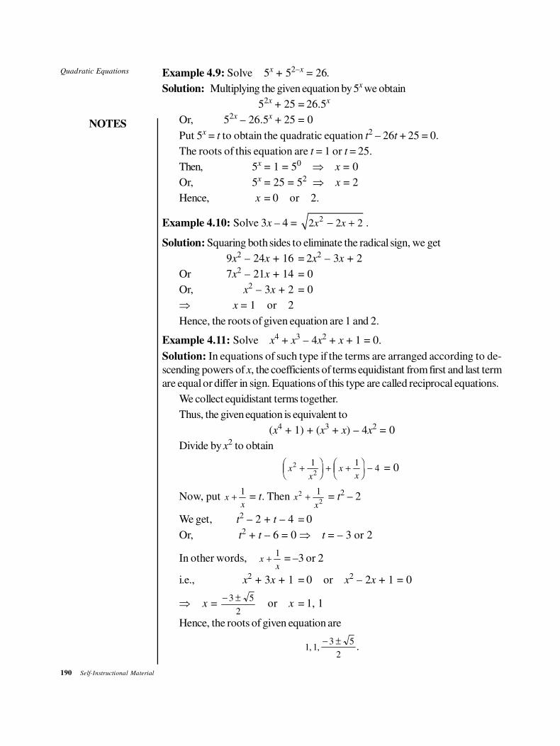
190 Self-Instructional Material
Quadratic Equations
NOTES
Example 4.9: Solve 5x + 52–x
= 26.
Solution: Multiplying the given equation by 5x we obtain
52x + 25 = 26.5x
Or, 52x – 26.5x + 25 = 0
Put 5x = t to obtain the quadratic equation t2 – 26t + 25 = 0.
The roots of this equation are t = 1 or t = 25.
Then, 5x = 1 = 50 ⇒ x = 0
Or, 5x = 25 = 52 ⇒ x = 2
Hence, x = 0 or 2.
Example 4.10: Solve 3x – 4 = 22 2 2x x− + .
Solution: Squaring both sides to eliminate the radical sign, we get
9x2 – 24x + 16 = 2x
2 – 3x + 2
Or 7x2 – 21x + 14 = 0
Or, x2 – 3x + 2 = 0
⇒ x = 1 or 2
Hence, the roots of given equation are 1 and 2.
Example 4.11: Solve x4 + x3 – 4x
2 + x + 1 = 0.
Solution: In equations of such type if the terms are arranged according to de-
scending powers of x, the coefficients of terms equidistant from first and last term
are equal or differ in sign. Equations of this type are called reciprocal equations.
We collect equidistant terms together.
Thus, the given equation is equivalent to
(x4 + 1) + (x3 + x) – 4x2 = 0
Divide by x2 to obtain
xx
xx
2
2
1 14+
FHG
IKJ + +FHGIKJ − = 0
Now, put xx
+1
= t. Then xx
2
2
1+ = t2 – 2
We get, t2 – 2 + t – 4 = 0
Or, t2 + t – 6 = 0 ⇒ t = – 3 or 2
In other words, xx
+1
= –3 or 2
i.e., x2 + 3x + 1 = 0 or x
2 – 2x + 1 = 0
⇒ x = − ±3 5
2or x = 1, 1
Hence, the roots of given equation are
1 13 5
2, ,
− ±.
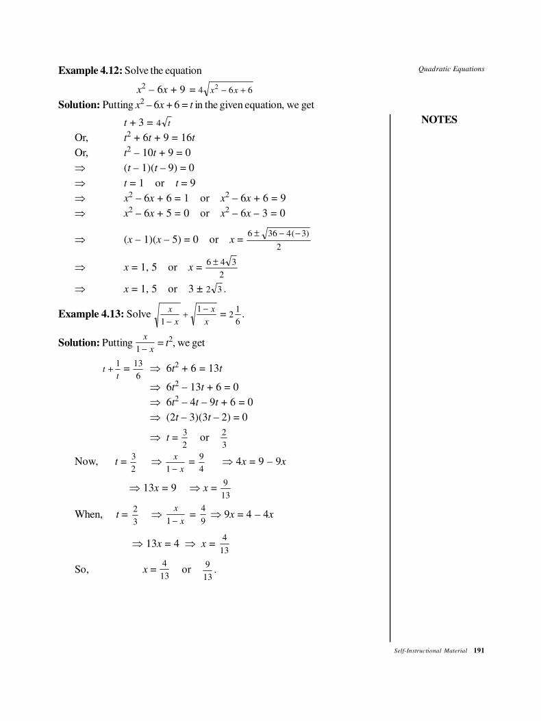
Quadratic Equations
NOTES
Self-Instructional Material 191
Example 4.12: Solve the equation
x2 – 6x + 9 = 4 6 62
x x− +
Solution: Putting x2 – 6x + 6 = t in the given equation, we get
t + 3 = 4 t
Or, t2 + 6t + 9 = 16t
Or, t2 – 10t + 9 = 0
⇒ (t – 1)(t – 9) = 0
⇒ t = 1 or t = 9
⇒ x2 – 6x + 6 = 1 or x
2 – 6x + 6 = 9
⇒ x2 – 6x + 5 = 0 or x
2 – 6x – 3 = 0
⇒ (x – 1)(x – 5) = 0 or x = 6 36 4 3
2
± − −( )
⇒ x = 1, 5 or x = 6 4 3
2
±
⇒ x = 1, 5 or 3 ± 2 3 .
Example 4.13: Solve x
x
x
x1
1
−+
− = 2
1
6.
Solution: Putting x
x1 − = t2, we get
tt
+1 =
13
6⇒ 6t
2 + 6 = 13t
⇒ 6t2 – 13t + 6 = 0
⇒ 6t2 – 4t – 9t + 6 = 0
⇒ (2t – 3)(3t – 2) = 0
⇒ t = 3
2or
2
3
Now, t = 3
2⇒
x
x1 − =
9
4⇒ 4x = 9 – 9x
⇒ 13x = 9 ⇒ x = 9
13
When, t =2
3⇒
1
x
x− =
4
9 ⇒ 9x = 4 – 4x
⇒ 13x = 4 ⇒ x = 4
13
So, x = 4
13or
9
13.
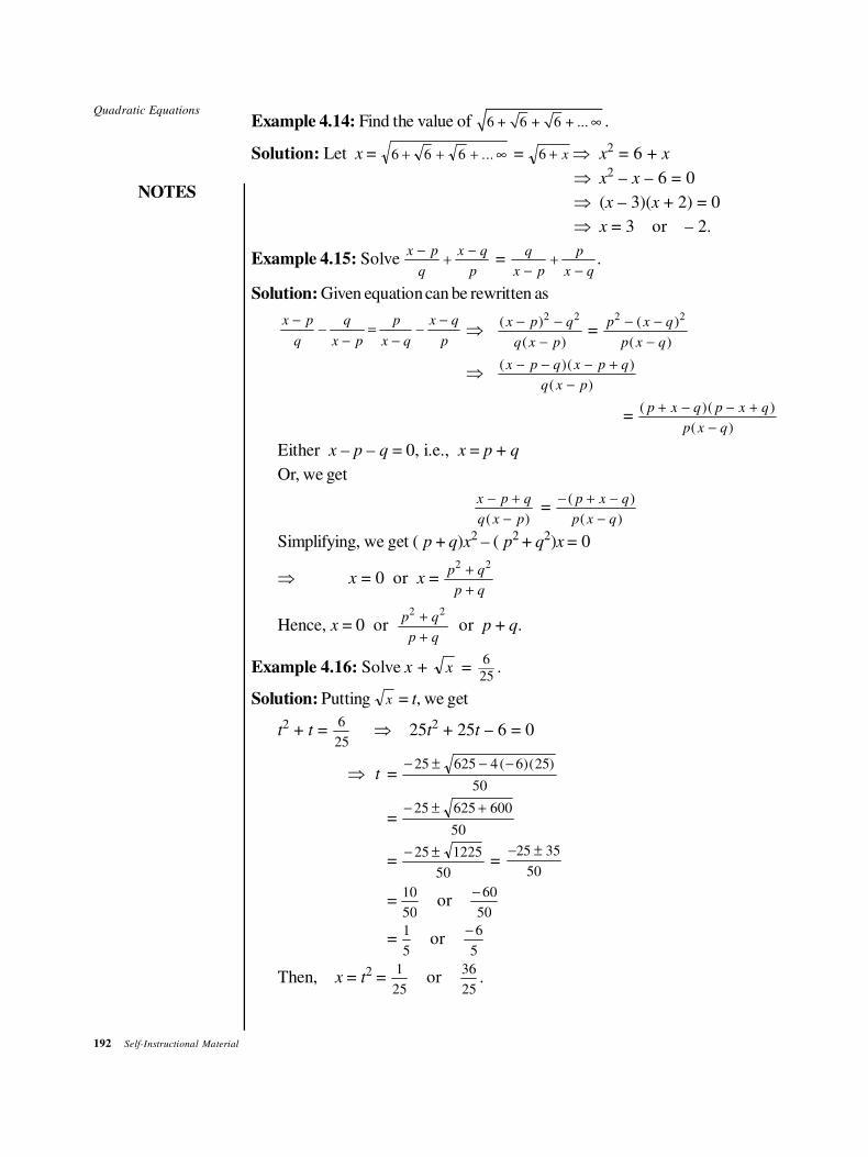
192 Self-Instructional Material
Quadratic Equations
NOTES
Example 4.14: Find the value of 6 6 6+ + + ... ∞ .
Solution: Let x = 6 6 6+ + + ∞... = 6 + x ⇒ x2 = 6 + x
⇒ x2 – x – 6 = 0
⇒ (x – 3)(x + 2) = 0
⇒ x = 3 or – 2.
Example 4.15: Solve x p
q
x q
p
−+
− =
q
x p
p
x q−+
−.
Solution: Given equation can be rewritten as
x p q p x q
q x p x q p
− −− = −
− −⇒
( )
( )
x p q
q x p
− −
−
2 2
= p x q
p x q
2 2− −
−
( )
( )
⇒( )( )
( )
x p q x p q
q x p
− − − +
−
= ( )( )
( )
p x q p x q
p x q
+ − − +
−
Either x – p – q = 0, i.e., x = p + q
Or, we get
x p q
q x p
− +
−( )=
− + −
−
( )
( )
p x q
p x q
Simplifying, we get ( p + q)x2 – ( p2 + q2)x = 0
⇒ x = 0 or x = p q
p q
2 2+
+
Hence, x = 0 orp q
p q
2 2+
+or p + q.
Example 4.16: Solve x + x = 6
25.
Solution: Putting x = t, we get
t2 + t =
6
25⇒ 25t
2 + 25t – 6 = 0
⇒ t = − ± − −25 625 4 6 25
50
( )( )
= − ± +25 625 600
50
= − ±25 1225
50 =
25 35
50
− ±
= 10
50or
− 60
50
= 1
5or
− 6
5
Then, x = t2 = 1
25or
36
25.
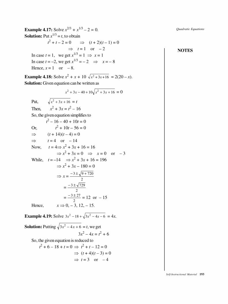
Quadratic Equations
NOTES
Self-Instructional Material 193
Example 4.17: Solve x2/3
+ x1/3
– 2 = 0.
Solution: Put x1/3 = t, to obtain
t2 + t – 2 = 0 ⇒ (t + 2)(t – 1) = 0
⇒ t = 1 or – 2
In case t = 1, we get x1/3 = 1 ⇒ x = 1
In case t = –2, we get x1/3 = – 2 ⇒ x = – 8
Hence, x = 1 or – 8.
Example 4.18: Solve x2 + x + 10 2 3 16x + x+ = 2(20 – x).
Solution: Given equation can be written as
x x x x2 23 40 10 3 16+ − + + + = 0
Put, x x2 3 16+ + = t
Then, x2 + 3x = t2 – 16
So, the given equation simplifies to
t2 – 16 – 40 + 10t = 0
Or, t2 + 10t – 56 = 0
⇒ (t + 14)(t – 4) = 0
⇒ t = 4 or – 14
Now, t = 4⇒ x2 + 3x + 16 = 16
⇒ x2 + 3x = 0 ⇒ x = 0 or – 3
While, t = –14 ⇒ x2 + 3x + 16 = 196
⇒ x2 + 3x – 180 = 0
⇒ x = − ± +3 9 720
2
= − ±3 729
2
= − ±3 27
2 = 12 or – 15
Hence, x ⇒ 0, – 3, 12, – 15.
Example 4.19: Solve 2 23 18 3 4 6x x x− + − − = 4x.
Solution: Putting 3 4 62x x− + = t, we get
3x2 – 4x = t2 + 6
So, the given equation is reduced to
t2 + 6 – 18 + t = 0 ⇒ t
2 + t – 12 = 0
⇒ (t + 4)(t – 3) = 0
⇒ t = 3 or – 4
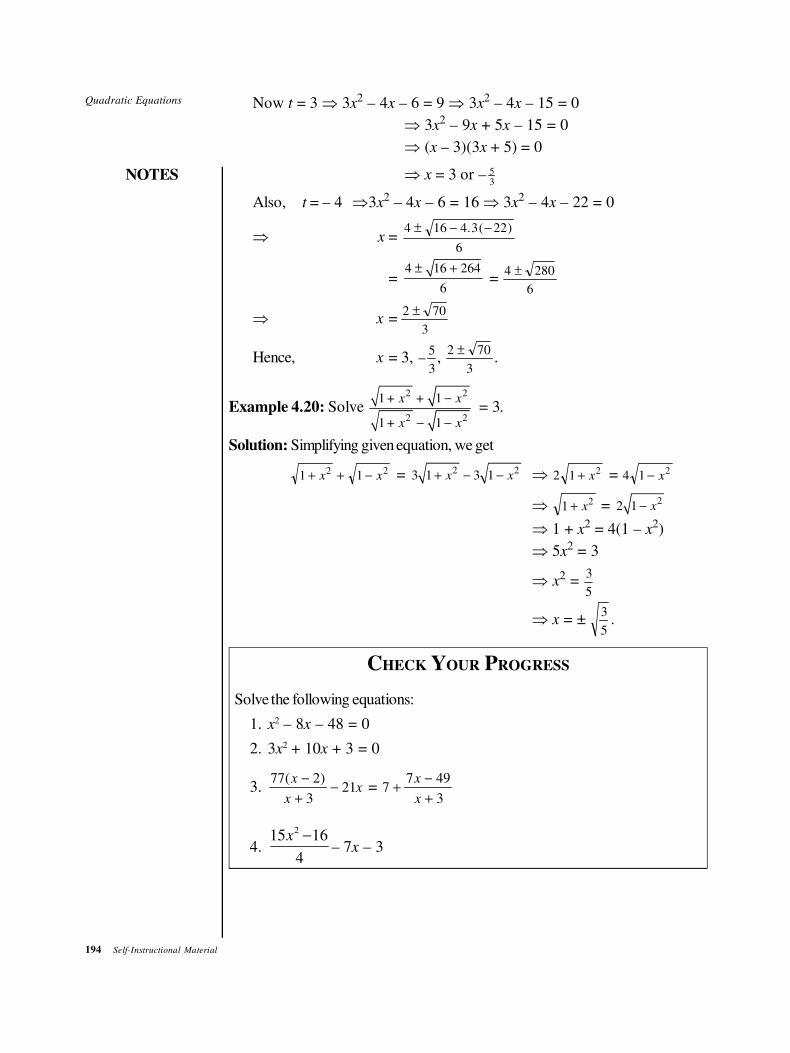
194 Self-Instructional Material
Quadratic Equations
NOTES
Now t = 3 ⇒ 3x2 – 4x – 6 = 9 ⇒ 3x
2 – 4x – 15 = 0
⇒ 3x2 – 9x + 5x – 15 = 0
⇒ (x – 3)(3x + 5) = 0
⇒ x = 3 or – 53
Also, t = – 4 ⇒3x2 – 4x – 6 = 16 ⇒ 3x
2 – 4x – 22 = 0
⇒ x = 4 16 4 3 22
6
± − −. ( )
= 4 16 264
6
± + =
4 280
6
±
⇒ x =2 70
3
±
Hence, x = 3, −5
3,
2 70
3
±.
Example 4.20: Solve 2 2
2 2
1 1
1 1
+ x + x
+ x x
−
− − = 3.
Solution: Simplifying given equation, we get
1 12 2+ + −x x = 2 23 1 3 1x x+ − − ⇒ 2 1 2+ x = 4 1 2− x
⇒ 1 2+ x = 22 1 x−
⇒ 1 + x2 = 4(1 – x2)
⇒ 5x2 = 3
⇒ x2 = 3
5
⇒ x = ±3
5.
CHECK YOUR PROGRESS
Solve the following equations:
1. x2 – 8x – 48 = 0
2. 3x2 + 10x + 3 = 0
3.77 2
321
( )x
xx
−
+− = 7
7 49
3+
−
+
x
x
4.
215 16
4
x −– 7x – 3
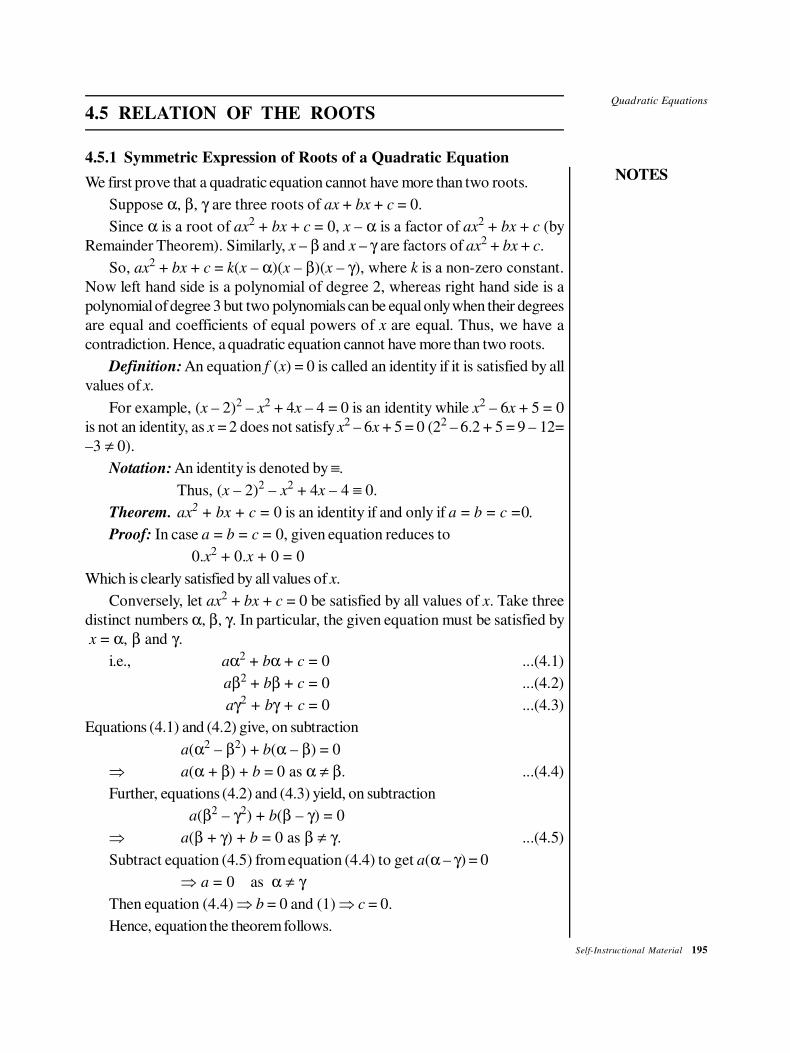
Quadratic Equations
NOTES
Self-Instructional Material 195
4.5 RELATION OF THE ROOTS
4.5.1 Symmetric Expression of Roots of a Quadratic Equation
We first prove that a quadratic equation cannot have more than two roots.
Suppose α, β, γ are three roots of ax + bx + c = 0.
Since α is a root of ax2 + bx + c = 0, x – α is a factor of ax
2 + bx + c (by
Remainder Theorem). Similarly, x – β and x – γ are factors of ax2 + bx + c.
So, ax2 + bx + c = k(x – α)(x – β)(x – γ), where k is a non-zero constant.
Now left hand side is a polynomial of degree 2, whereas right hand side is a
polynomial of degree 3 but two polynomials can be equal only when their degrees
are equal and coefficients of equal powers of x are equal. Thus, we have a
contradiction. Hence, a quadratic equation cannot have more than two roots.
Definition: An equation f (x) = 0 is called an identity if it is satisfied by all
values of x.
For example, (x – 2)2 – x2 + 4x – 4 = 0 is an identity while x2 – 6x + 5 = 0
is not an identity, as x = 2 does not satisfy x2 – 6x + 5 = 0 (22 – 6.2 + 5 = 9 – 12=
–3 ≠ 0).
Notation: An identity is denoted by ≡.
Thus, (x – 2)2 – x2 + 4x – 4 ≡ 0.
Theorem. ax2 + bx + c = 0 is an identity if and only if a = b = c =0.
Proof: In case a = b = c = 0, given equation reduces to
0.x2 + 0.x + 0 = 0
Which is clearly satisfied by all values of x.
Conversely, let ax2 + bx + c = 0 be satisfied by all values of x. Take three
distinct numbers α, β, γ. In particular, the given equation must be satisfied by
x = α, β and γ.
i.e., aα2 + bα + c = 0 ...(4.1)
aβ2 + bβ + c = 0 ...(4.2)
aγ2 + bγ + c = 0 ...(4.3)
Equations (4.1) and (4.2) give, on subtraction
a(α2 – β2) + b(α – β) = 0
⇒ a(α + β) + b = 0 as α ≠ β. ...(4.4)
Further, equations (4.2) and (4.3) yield, on subtraction
a(β2 – γ2) + b(β – γ) = 0
⇒ a(β + γ) + b = 0 as β ≠ γ. ...(4.5)
Subtract equation (4.5) from equation (4.4) to get a(α – γ) = 0
⇒ a = 0 as α ≠ γ
Then equation (4.4) ⇒ b = 0 and (1) ⇒ c = 0.
Hence, equation the theorem follows.
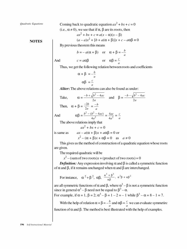
196 Self-Instructional Material
Quadratic Equations
NOTES
Coming back to quadratic equation ax2 + bx + c = 0
(i.e., α ≠ 0), we see that if α, β are its roots, then
ax2 + bx + c ≡ a(x – α)(x – β)
(a – a)x2 + [b + a(α + β)]x + c – aαβ ≡ 0
By previous theorem this means
b = – a(α + β) or α + β = –b
a
And c = aαβ or αβ = c
a
Thus, we get the following relation between roots and coefficients
α + β = −b
a
αβ =c
a
Aliter: The above relations can also be found as under:
Take, α =− + −b b ac
a
2 4
2and β =
− − −b b ac
a
2 4
2
Then, α + β =2
2
b
a
− =
−b
a
And αβ =b b ac
a
2 2
2
4
4
− −( ) =
4
4 2
ac
a
= c
a
The above relations imply that
ax2 + bx + c = 0
is same as ax – a(α + β)x + aαβ = 0 or
x2 – (α + β)x + αβ = 0 as a ≠ 0
This gives us the method of construction of a quadratic equation whose roots
are given.
The required quadratic will be
x2 – (sum of two roots)x + (product of two roots) = 0
Definition: Any expression involving α and β is called a symmetric function
of α and β, if it remains unchanged when α and β are interchanged.
For instance, α 2 + β 2, αβ, 3 3
2 2α β, α β αβ
αβ
++
are all symmetric functions of α and β, where α3 – β is not a symmetric function
since in general α3 – β need not be equal to β3 – α.
For example, if α = 1, β = 2; α3 – β = 1 – 2 = – 1 while β3 – α = 8 – 1 = 7.
With the help of relation α + β = −b
a and αβ =
c
a we can evaluate symmetirc
function of α and β. The method is best illustrated with the help of examples.
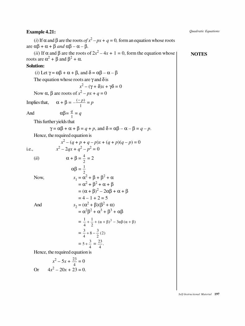
Quadratic Equations
NOTES
Self-Instructional Material 197
Example 4.21:
(i) If α and β are the roots of x2 – px + q = 0, form an equation whose roots
are αβ + α + β and αβ – α – β.
(ii) If α and β are the roots of 2x2 – 4x + 1 = 0, form the equation whose
roots are α2 + β and β2
+ α.
Solution:
(i) Let γ = αβ + α + β, and δ = αβ – α – β
The equation whose roots are γ and δ is
x2 – (γ + δ)x + γδ = 0
Now α, β are roots of x2 – px + q = 0
Implies that, α + β = −−( )p
1 = p
And αβ= q
1 = q
This further yields that
γ = αβ + α + β = q + p, and δ = αβ – α – β = q – p.
Hence, the required equation is
x2 – (q + p + q – p)x + (q + p)(q – p) = 0
i.e., x2 – 2qx + q2 – p2 = 0
(ii) α + β = 4
2 = 2
αβ = 1
2
Now, s1
= α2 + β + β2 + α
= α2 + β2 + α + β
= (α + β)2 – 2αβ + α + β
= 4 – 1 + 2 = 5
And s2
= (α2 + β)(β2 + α)
= α2β2 + α3 + β3 + αβ
= 1 1
(α β) 3αβ (α β)4 2
3+ + + − +
= 3
48
3
22+ − ( )
= 53
4+ =
23
4.
Hence, the required equation is
x2 – 5x +
23
4= 0
Or 4x2 – 20x + 23 = 0.
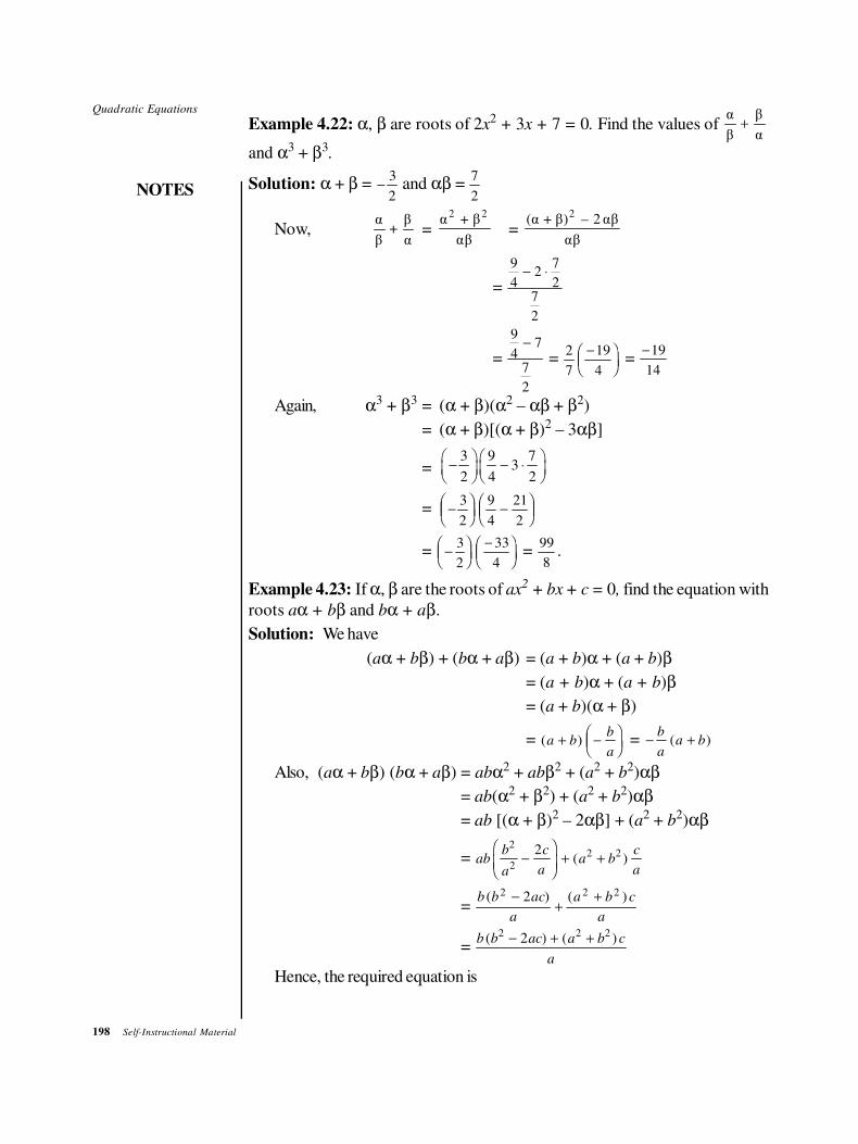
198 Self-Instructional Material
Quadratic Equations
NOTES
Example 4.22: α, β are roots of 2x2 + 3x + 7 = 0. Find the values of
α β
β α+
and α3 + β3.
Solution: α + β = −3
2 and αβ =
7
2
Now,α β
+β α
= 2 2α + β
αβ=
2(α + β) – 2 αβ
αβ
=
9
42
7
27
2
− ⋅
=
9
47
7
2
− =
2
7
19
4
−FHGIKJ =
−19
14
Again, α3 + β3 = (α + β)(α2 – αβ + β2)
= (α + β)[(α + β)2 – 3αβ]
=3 9 7
32 4 2
− − ⋅
= −FHGIKJ −FHG
IKJ
3
2
9
4
21
2
= −FHGIKJ
−FHGIKJ
3
2
33
4 =
99
8.
Example 4.23: If α, β are the roots of ax2 + bx + c = 0, find the equation with
roots aα + bβ and bα + aβ.
Solution: We have
(aα + bβ) + (bα + aβ) = (a + b)α + (a + b)β
= (a + b)α + (a + b)β
= (a + b)(α + β)
= ( )a bb
a+ −FHGIKJ = − +
b
aa b( )
Also, (aα + bβ) (bα + aβ) = abα2 + abβ2 + (a2 + b2)αβ
= ab(α2 + β2) + (a2 + b2)αβ
= ab [(α + β)2 – 2αβ] + (a2 + b2)αβ
= abb
a
c
aa b
c
a
2
2
2 22−
FHG
IKJ + +( )
= b b ac
a
a b c
a
( ) ( )2 2 22−+
+
= b b ac a b c
a
( ) ( )2 2 22− + +
Hence, the required equation is
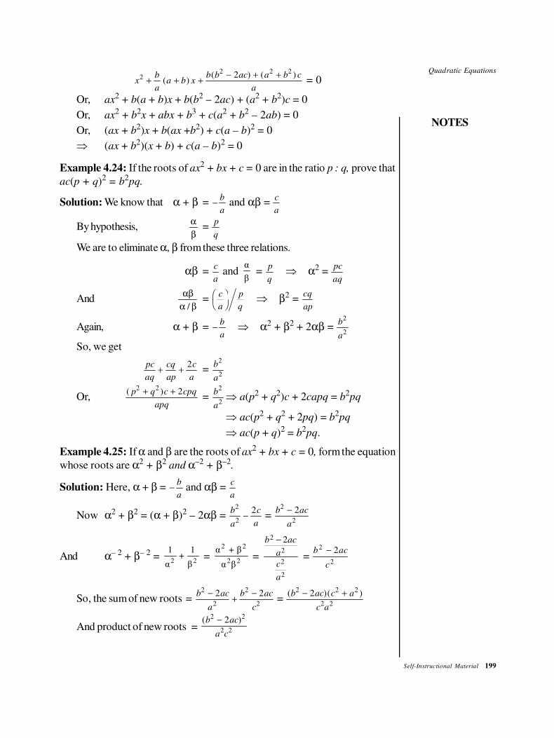
Quadratic Equations
NOTES
Self-Instructional Material 199
xb
aa b x
b b ac a b c
a
22 2 22
+ + +− + +
( )( ) ( )
= 0
Or, ax2 + b(a + b)x + b(b2 – 2ac) + (a2 + b2)c = 0
Or, ax2 + b2
x + abx + b3 + c(a2 + b2 – 2ab) = 0
Or, (ax + b2)x + b(ax +b2) + c(a – b)2 = 0
⇒ (ax + b2)(x + b) + c(a – b)2 = 0
Example 4.24: If the roots of ax2 + bx + c = 0 are in the ratio p : q, prove that
ac(p + q)2 = b
2pq.
Solution: We know that α + β = −b
a and αβ =
c
a
By hypothesis,α
β=
p
q
We are to eliminate α, β from these three relations.
αβ = c
a and
α
β =
p
q⇒ α2 =
pc
aq
Andαβ
α β/=
c
a
p
q
FHIK ⇒ β2 =
cq
ap
Again, α + β = −b
a⇒ α2 + β2 + 2αβ =
b
a
2
2
So, we get
pc
aq
cq
ap
c
a+ +
2=
b
a
2
2
Or,( )p q c cpq
apq
2 2 2+ +=
b
a
2
2⇒ a(p2 + q2)c + 2capq = b2
pq
⇒ ac(p2 + q2 + 2pq) = b2pq
⇒ ac(p + q)2 = b2pq.
Example 4.25: If α and β are the roots of ax2 + bx + c = 0, form the equation
whose roots are α2 + β2
and α–2 + β–2
.
Solution: Here, α + β = −b
a and αβ =
c
a
Now α2 + β2 = (α + β)2 – 2αβ = b
a
c
a
2
2
2− =
b ac
a
2
2
2−
And α– 2 + β– 2 = 2 2
1 1+
α β =
2 2
2 2
α + β
α β =
2
2
2
2
2b ac
a
c
a
−
= b ac
c
2 − 2
2
So, the sum of new roots = b ac
a
b ac
c
2
2
2
2
2 2−+
− =
( )( )b ac c a
c a
2 2 2
2 2
2− +
And product of new roots = ( )b ac
a c
2 2
2 2
2−
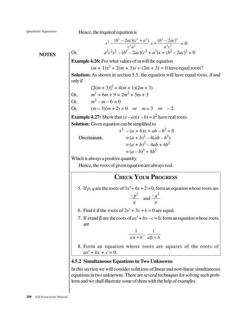
200 Self-Instructional Material
Quadratic Equations
NOTES
Hence, the required equation is
2 2 2 2 22
2 2 2 2
( 2 )( ) ( 2 )b ac c a b acx x
c a a c
− + −− + = 0
Or, a2c
2x
2 – (b2 – 2ac)(c2 + a2)x + (b2 – 2ac)2 = 0
Example 4.26: For what values of m will the equation
(m + 1)x2 + 2(m + 3)x + (2m + 3) = 0 have equal roots?
Solution: As shown in section 5.5, the equation will have equal roots, if and
only if
[2(m + 3)]2 = 4(m + 1)(2m + 3)
Or, m2 + 6m + 9 = 2m
2 + 5m + 3
Or, m2 – m – 6 = 0
Or, (m – 3)(m + 2) = 0 or m = 3 or – 2.
Example 4.27: Show that (x – a)(x – b) = h2 have real roots.
Solution: Given equation can be simplified to
x2 – (a + b)x + ab – h
2 = 0
Discriminant, = (a + b)2 – 4(ab – h2)
= (a + b)2 – 4ab + 4h2
= (a – b)2 + 4h2
Which is always a positive quantity.
Hence, the roots of given equation are always real.
CHECK YOUR PROGRESS
5. If p, q are the roots of 3x2 + 6x + 2 = 0, form an equation whose roots are
− p
q
2
and −q
p
2
6. Find k if the roots of 2x2 + 3x + k = 0 are equal.
7. If α and β are the roots of ax2 + bx – c = 0, form an equation whose roots
are
1 1,
α βa b a b+ +
8. Form an equation whose roots are squares of the roots of
ax2 + bx + c = 0.
4.5.2 Simultaneous Equations in Two Unknowns
In this section we will consider solutions of linear and non-linear simultaneous
equations in two unknowns. There are several techniques for solving such prob-
lems and we shall illustrate some of them with the help of examples.
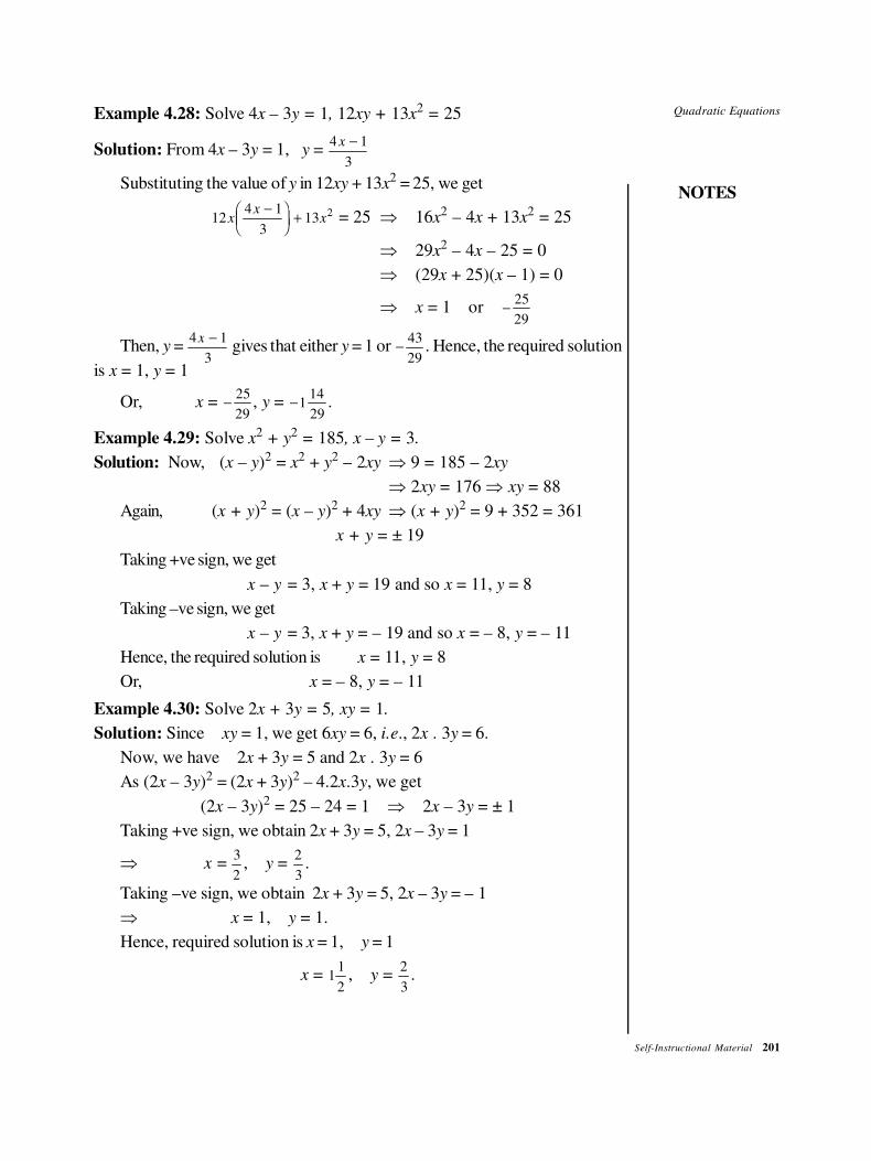
Quadratic Equations
NOTES
Self-Instructional Material 201
Example 4.28: Solve 4x – 3y = 1, 12xy + 13x2 = 25
Solution: From 4x – 3y = 1, y = 4 1
3
x −
Substituting the value of y in 12xy + 13x2 = 25, we get
124 1
313 2
xx
x−F
HGIKJ + = 25 ⇒ 16x
2 – 4x + 13x2 = 25
⇒ 29x2 – 4x – 25 = 0
⇒ (29x + 25)(x – 1) = 0
⇒ x = 1 or −25
29
Then, y = 4 1
3
x − gives that either y = 1 or −
43
29. Hence, the required solution
is x = 1, y = 1
Or, x = −25
29, y = −1
14
29.
Example 4.29: Solve x2 + y
2 = 185, x – y = 3.
Solution: Now, (x – y)2 = x2 + y2 – 2xy ⇒ 9 = 185 – 2xy
⇒ 2xy = 176 ⇒ xy = 88
Again, (x + y)2 = (x – y)2 + 4xy ⇒ (x + y)2 = 9 + 352 = 361
x + y = ± 19
Taking +ve sign, we get
x – y = 3, x + y = 19 and so x = 11, y = 8
Taking –ve sign, we get
x – y = 3, x + y = – 19 and so x = – 8, y = – 11
Hence, the required solution is x = 11, y = 8
Or, x = – 8, y = – 11
Example 4.30: Solve 2x + 3y = 5, xy = 1.
Solution: Since xy = 1, we get 6xy = 6, i.e., 2x . 3y = 6.
Now, we have 2x + 3y = 5 and 2x . 3y = 6
As (2x – 3y)2 = (2x + 3y)2 – 4.2x.3y, we get
(2x – 3y)2 = 25 – 24 = 1 ⇒ 2x – 3y = ± 1
Taking +ve sign, we obtain 2x + 3y = 5, 2x – 3y = 1
⇒ x =3
2, y =
2
3.
Taking –ve sign, we obtain 2x + 3y = 5, 2x – 3y = – 1
⇒ x = 1, y = 1.
Hence, required solution is x = 1, y = 1
x = 11
2, y =
2
3.
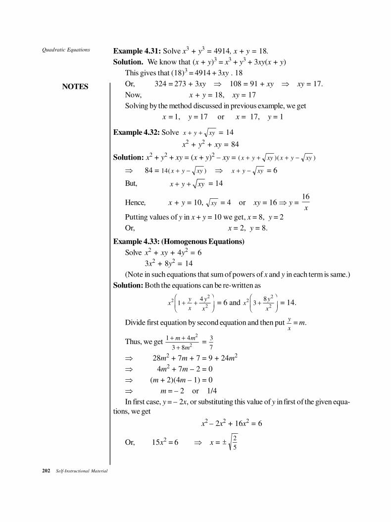
202 Self-Instructional Material
Quadratic Equations
NOTES
Example 4.31: Solve x3 + y
3 = 4914, x + y = 18.
Solution. We know that (x + y)3 = x3 + y3 + 3xy(x + y)
This gives that (18)3 = 4914 + 3xy . 18
Or, 324 = 273 + 3xy ⇒ 108 = 91 + xy ⇒ xy = 17.
Now, x + y = 18, xy = 17
Solving by the method discussed in previous example, we get
x = 1, y = 17 or x = 17, y = 1
Example 4.32: Solve x y xy+ + = 14
x2 + y
2 + xy = 84
Solution: x2 + y2 + xy = (x + y)2 – xy = ( )( )x y xy x y xy+ + + −
⇒ 84 = 14( )x y xy+ − ⇒ x y xy+ − = 6
But, x y xy+ + = 14
Hence, x + y = 10, xy = 4 or xy = 16 ⇒ y = 16
x
Putting values of y in x + y = 10 we get, x = 8, y = 2
Or, x = 2, y = 8.
Example 4.33: (Homogenous Equations)
Solve x2 + xy + 4y
2 = 6
3x2 + 8y
2 = 14
(Note in such equations that sum of powers of x and y in each term is same.)
Solution: Both the equations can be re-written as
xy
x
y
x
22
21
4+ +FHG
IKJ = 6 and x
y
x
22
23
8+FHG
IKJ = 14.
Divide first equation by second equation and then put y
x = m.
Thus, we get1 4
3 8
2
2
+ +
+
m m
m=
3
7
⇒ 28m2 + 7m + 7 = 9 + 24m
2
⇒ 4m2 + 7m – 2 = 0
⇒ (m + 2)(4m – 1) = 0
⇒ m = – 2 or 1/4
In first case, y = – 2x, or substituting this value of y in first of the given equa-
tions, we get
x2 – 2x
2 + 16x2 = 6
Or, 15x2 = 6 ⇒ x = ±
2
5
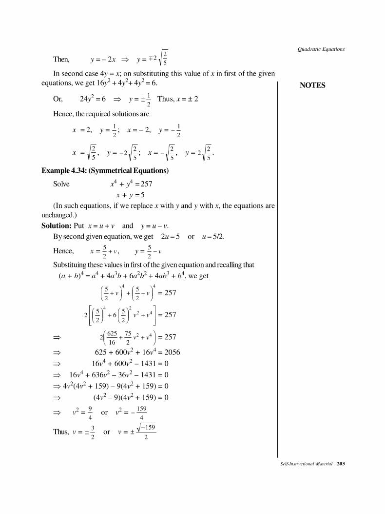
Quadratic Equations
NOTES
Self-Instructional Material 203
Then, y = – 2x ⇒ y = ∓22
5
In second case 4y = x; on substituting this value of x in first of the given
equations, we get 16y2 + 4y
2+ 4y2 = 6.
Or, 24y2 = 6 ⇒ y = ±
1
2 Thus, x = ± 2
Hence, the required solutions are
x = 2, y = 1
2; x = – 2, y = −
1
2
x =2
5, y = − 2
2
5; x = −
2
5, y = 2
2
5.
Example 4.34: (Symmetrical Equations)
Solve x4 + y
4=257
x + y =5
(In such equations, if we replace x with y and y with x, the equations are
unchanged.)
Solution: Put x = u + v and y = u – v.
By second given equation, we get 2u = 5 or u = 5/2.
Hence, x =5
2+ v , y =
5
2− v
Substituing these values in first of the given equation and recalling that
(a + b)4 = a4 + 4a3b + 6a
2b
2 + 4ab3 + b4, we get
5
2
5
2
4 4
+FHGIKJ + −FHGIKJv v = 257
25
26
5
2
4 22 4F
HGIKJ +FHGIKJ +
LNMM
OQPP
v v = 257
⇒ 2625
16
75
2
2 4+ +FHG
IKJv v = 257
⇒ 625 + 600v2 + 16v
4 = 2056
⇒ 16v4 + 600v
2 – 1431 = 0
⇒ 16v4 + 636v
2 – 36v2 – 1431 = 0
⇒ 4v2(4v
2 + 159) – 9(4v2 + 159) = 0
⇒ (4v2 – 9)(4v
2 + 159) = 0
⇒ v2 =
9
4or v
2 = −159
4
Thus, v = ±3
2or v = ±
−159
2
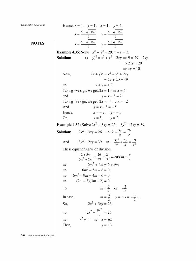
204 Self-Instructional Material
Quadratic Equations
NOTES
Hence, x = 4, y = 1; x = 1, y = 4
x = 5 159
2
+ −, y =
5 159
2
− −
x = 5 159
2
− −, y =
5 159
2
+ −
Example 4.35: Solve x2 + y
2= 29, x – y = 3.
Solution: (x – y)2 = x2 + y2 – 2xy ⇒ 9 = 29 – 2xy
⇒ 2xy = 20
⇒ xy = 10
Now, (x + y)2 = x2 + y2 + 2xy
= 29 + 20 = 49
⇒ x + y = ± 7
Taking +ve sign, we get, 2x = 10 ⇒ x = 5
and y = x – 3 = 2
Taking –ve sign, we get 2x = –4 ⇒ x = –2
And y = x – 3 = – 5
Hence, x = – 2, y = – 5
Or, x = 5, y = 2
Example 4.36: Solve 2x2 + 3xy = 26, 3y
2 + 2xy = 39.
Solution: 2x2 + 3xy = 26 ⇒ 2
3y
x+ =
262
x
And 3y2 + 2xy = 39 ⇒
3 22
2
y
x
y
x+ =
392
x
These equations give on division,
2 3
3 22
+
+
m
m m =
26
39 =
2
3, where m =
y
x
⇒ 6m2 + 4m = 6 + 9m
⇒ 6m2 – 5m – 6 = 0
⇒ 6m2 – 9m + 4m – 6 = 0
⇒ (2m – 3)(3m + 2) = 0
⇒ m = 3
2or −
2
3
In case, m = 3
2, y = mx = −
3
2x ,
So, 2x2 + 3xy = 26
⇒ 2x2 +
29
2
x= 26
⇒ x2 = 4 ⇒ x = ±2
Then, y = ±3
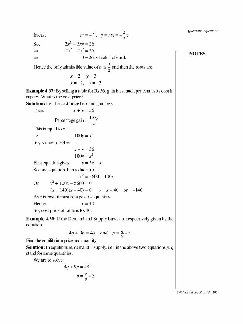
Quadratic Equations
NOTES
Self-Instructional Material 205
In case m = –2
3, y = mx = –
2
3x
So, 2x2 + 3xy = 26
⇒ 2x2 – 2x
2 = 26
⇒ 0 = 26, which is absurd.
Hence the only admissible value of m is 3
2 and then the roots are
x = 2, y = 3
x = –2, y = –3.
Example 4.37: By selling a table for Rs 56, gain is as much per cent as its cost in
rupees. What is the cost price?
Solution: Let the cost price be x and gain be y
Then, x + y = 56
Percentage gain = 100y
x
This is equal to x
i.e., 100y = x2
So, we are to solve
x + y = 56
100y = x2
First equation gives y = 56 – x
Second equation then reduces to
x2 = 5600 – 100x
Or, x2 + 100x – 5600 = 0
(x + 140)(x – 40) = 0 ⇒ x = 40 or –140
As x is cost, it must be a positive quantity.
Hence, x = 40
So, cost price of table is Rs 40.
Example 4.38: If the Demand and Supply Laws are respectively given by the
equation
4q + 9p = 48 and p = q
92+
Find the equilibrium price and quantity.
Solution: In equilibrium, demand = supply, i.e., in the above two equations p, q
stand for same quantities.
We are to solve
4q + 9p = 48
p = q
92+
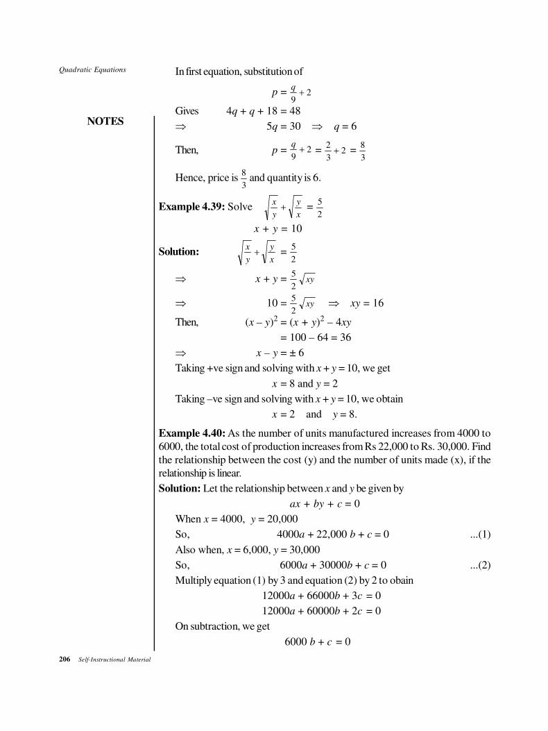
206 Self-Instructional Material
Quadratic Equations
NOTES
In first equation, substitution of
p = q
92+
Gives 4q + q + 18 = 48
⇒ 5q = 30 ⇒ q = 6
Then, p = q
92+ =
2
32+ =
8
3
Hence, price is 8
3 and quantity is 6.
Example 4.39: Solvex
y
y
x+ =
5
2
x + y = 10
Solution:x
y
y
x+ =
5
2
⇒ x + y = 5
2xy
⇒ 10 = 5
2xy ⇒ xy = 16
Then, (x – y)2 = (x + y)2 – 4xy
= 100 – 64 = 36
⇒ x – y = ± 6
Taking +ve sign and solving with x + y = 10, we get
x = 8 and y = 2
Taking –ve sign and solving with x + y = 10, we obtain
x = 2 and y = 8.
Example 4.40: As the number of units manufactured increases from 4000 to
6000, the total cost of production increases from Rs 22,000 to Rs. 30,000. Find
the relationship between the cost (y) and the number of units made (x), if the
relationship is linear.
Solution: Let the relationship between x and y be given by
ax + by + c = 0
When x = 4000, y = 20,000
So, 4000a + 22,000 b + c = 0 ...(1)
Also when, x = 6,000, y = 30,000
So, 6000a + 30000b + c = 0 ...(2)
Multiply equation (1) by 3 and equation (2) by 2 to obain
12000a + 66000b + 3c = 0
12000a + 60000b + 2c = 0
On subtraction, we get
6000 b + c = 0
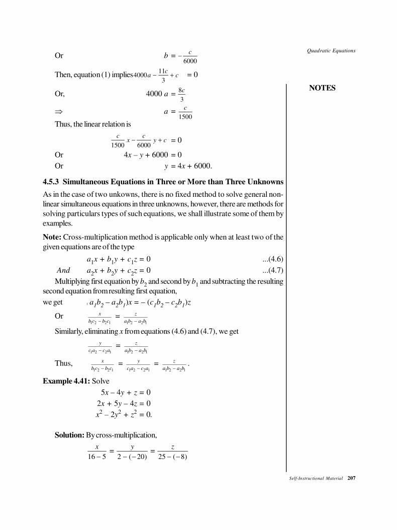
Quadratic Equations
NOTES
Self-Instructional Material 207
Or b = −c
6000
Then, equation (1) implies400011
3a
cc− + = 0
Or, 4000 a = 8
3
c
⇒ a = c
1500
Thus, the linear relation is
1500 6000
c cx y c− + = 0
Or 4x – y + 6000 = 0
Or y = 4x + 6000.
4.5.3 Simultaneous Equations in Three or More than Three Unknowns
As in the case of two unkowns, there is no fixed method to solve general non-
linear simultaneous equations in three unknowns, however, there are methods for
solving particulars types of such equations, we shall illustrate some of them by
examples.
Note: Cross-multiplication method is applicable only when at least two of the
given equations are of the type
a1x + b
1y + c
1z = 0 ...(4.6)
And a2x + b
2y + c
2z = 0 ...(4.7)
Multiplying first equation by b2 and second by b
1 and subtracting the resulting
second equation from resulting first equation,
we get ( a1b
2 – a
2b
1)x = – (c
1b
2 – c
2b
1)z
Or1 2 2 1
x
b c b c− =
1 2 2 1
z
a b a b−
Similarly, eliminating x from equations (4.6) and (4.7), we get
1 2 2 1
y
c a c a− =
1 2 2 1
z
a b a b−
Thus, 1 2 2 1
x
b c b c− =
1 2 2 1
y
c a c a− =
1 2 2 1
z
a b a b−.
Example 4.41: Solve
5x – 4y + z = 0
2x + 5y – 4z = 0
x2 – 2y
2 + z
2= 0.
Solution: By cross-multiplication,
x
16 5− =
y
2 20− −( ) =
z
25 8− −( )
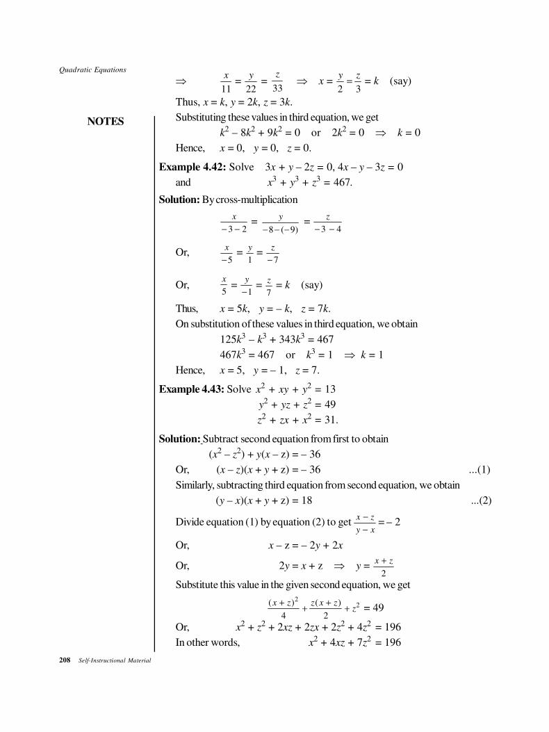
208 Self-Instructional Material
Quadratic Equations
NOTES
⇒x
11 =
y
22 =
33
z⇒ x =
y z
2 3= = k (say)
Thus, x = k, y = 2k, z = 3k.
Substituting these values in third equation, we get
k2 – 8k
2 + 9k2 = 0 or 2k
2 = 0 ⇒ k = 0
Hence, x = 0, y = 0, z = 0.
Example 4.42: Solve 3x + y – 2z = 0, 4x – y – 3z = 0
and x3 + y
3 + z
3 = 467.
Solution: By cross-multiplication
x
− −3 2 =
8 ( 9)
y
− − − =
z
− −3 4
Or,x
−5 =
y
1 =
z
− 7
Or,x
5 =
y
−1 =
z
7 = k (say)
Thus, x = 5k, y = – k, z = 7k.
On substitution of these values in third equation, we obtain
125k3 – k3 + 343k
3 = 467
467k3 = 467 or k
3 = 1 ⇒ k = 1
Hence, x = 5, y = – 1, z = 7.
Example 4.43: Solve x2 + xy + y
2= 13
y2 + yz + z
2= 49
z2 + zx + x
2= 31.
Solution: Subtract second equation from first to obtain
(x2 – z2) + y(x – z) = – 36
Or, (x – z)(x + y + z) = – 36 ...(1)
Similarly, subtracting third equation from second equation, we obtain
(y – x)(x + y + z) = 18 ...(2)
Divide equation (1) by equation (2) to get x z
y x
−
− = – 2
Or, x – z = – 2y + 2x
Or, 2y = x + z ⇒ y = x z+
2
Substitute this value in the given second equation, we get
( ) ( )x z z x zz
++
++
22
4 2 = 49
Or, x2 + z2 + 2xz + 2zx + 2z
2 + 4z2 = 196
In other words, x2 + 4xz + 7z
2 = 196
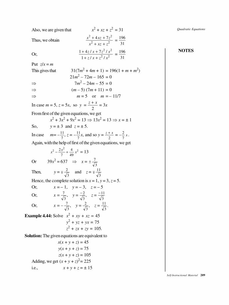
Quadratic Equations
NOTES
Self-Instructional Material 209
Also, we are given that x2 + xz + z2 = 31
Thus, we obtainx xz z
x xz z
2 2
2 2
4 7+ +
+ +=
196
31
Or,1 4 7
1
2 2
2 2
+ +
+ +
z x z x
z x z x
/ /
/ /=
196
31
Put z/x = m
This gives that 31(7m2 + 4m + 1) = 196(1 + m + m2)
21m2 – 72m – 165 = 0
⇒ 7m2 – 24m – 55 = 0
⇒ (m – 5) (7m + 11) = 0
⇒ m = 5 or m = – 11/7
In case m = 5, z = 5x, so y = z x+
2 = 3x
From first of the given equations, we get
x2 + 3x
2 + 9x2 = 13 ⇒ 13x
2 = 13 ⇒ x = ± 1
So, y = ± 3 and z = ± 5.
In case m= −11
7, z = −
11
7x, and so y =
z x+
2 = −
2
7x .
Again, with the help of first of the given equations, we get
xx
x2
222
7
4
49− + = 13
Or 39x2 = 637 ⇒ x = ±
7
3
Then, y = ∓2
3and z = ∓
11
3
Hence, the complete solution is x = 1, y = 3, z = 5.
Or, x = – 1, y = – 3, z = – 5
Or, x =7
3, y =
− 2
3, z =
−11
3
Or, x = −7
3, y =
2
3, z =
11
3.
Example 4.44: Solve x2 + xy + xz = 45
y2 + yz + yx = 75
z2 + zx + zy = 105.
Solution: The given equations are equivalent to
x(x + y + z) = 45
y(x + y + z) = 75
z(x + y + z) = 105
Adding, we get (x + y + z)2= 225
i.e., x + y + z = ± 15
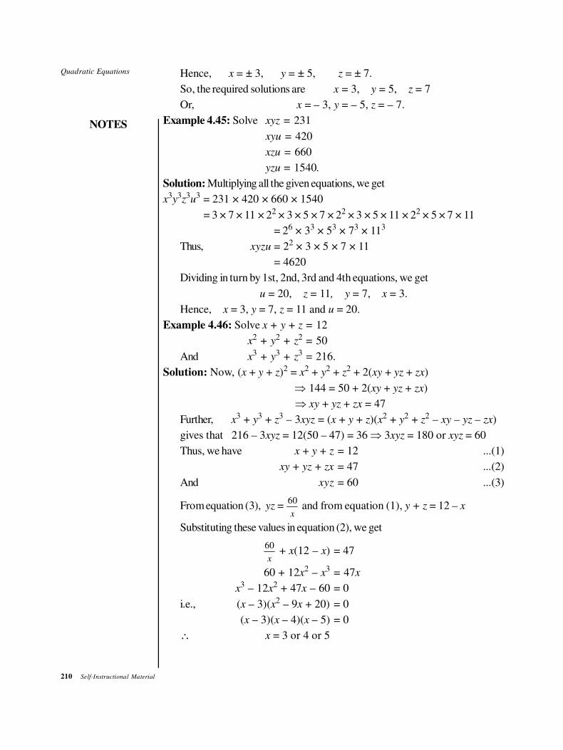
210 Self-Instructional Material
Quadratic Equations
NOTES
Hence, x = ± 3, y = ± 5, z = ± 7.
So, the required solutions are x = 3, y = 5, z = 7
Or, x = – 3, y = – 5, z = – 7.
Example 4.45: Solve xyz = 231
xyu = 420
xzu = 660
yzu = 1540.
Solution: Multiplying all the given equations, we get
x3y
3z
3u
3 = 231 × 420 × 660 × 1540
= 3 × 7 × 11 × 22 × 3 × 5 × 7 × 22 × 3 × 5 × 11 × 22 × 5 × 7 × 11
= 26 × 33 × 53 × 73 × 113
Thus, xyzu = 22 × 3 × 5 × 7 × 11
= 4620
Dividing in turn by 1st, 2nd, 3rd and 4th equations, we get
u = 20, z = 11, y = 7, x = 3.
Hence, x = 3, y = 7, z = 11 and u = 20.
Example 4.46: Solve x + y + z = 12
x2 + y
2 + z
2= 50
And x3 + y
3 + z
3= 216.
Solution: Now, (x + y + z)2 = x2 + y2 + z2 + 2(xy + yz + zx)
⇒ 144 = 50 + 2(xy + yz + zx)
⇒ xy + yz + zx = 47
Further, x3 + y3 + z3 – 3xyz = (x + y + z)(x2 + y2 + z2 – xy – yz – zx)
gives that 216 – 3xyz = 12(50 – 47) = 36 ⇒ 3xyz = 180 or xyz = 60
Thus, we have x + y + z = 12 ...(1)
xy + yz + zx = 47 ...(2)
And xyz = 60 ...(3)
From equation (3), yz = 60
x and from equation (1), y + z = 12 – x
Substituting these values in equation (2), we get
60
x + x(12 – x) = 47
60 + 12x2 – x3 = 47x
x3 – 12x
2 + 47x – 60 = 0
i.e., (x – 3)(x2 – 9x + 20) = 0
(x – 3)(x – 4)(x – 5) = 0
∴ x = 3 or 4 or 5
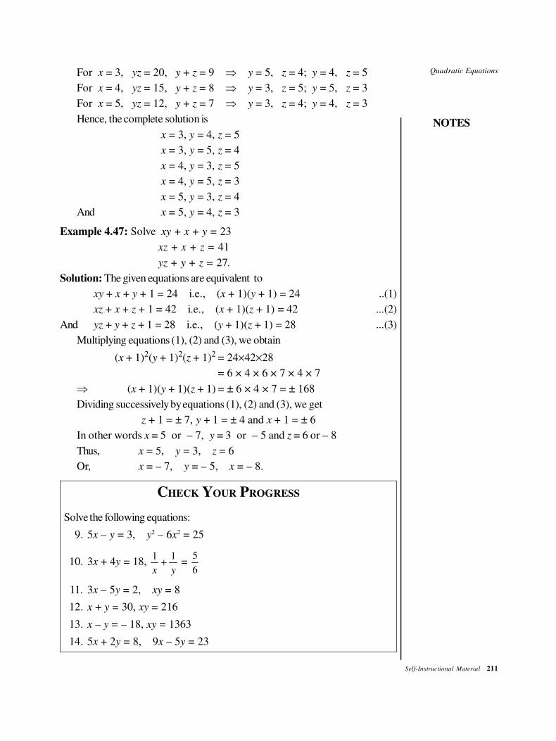
Quadratic Equations
NOTES
Self-Instructional Material 211
For x = 3, yz = 20, y + z = 9 ⇒ y = 5, z = 4; y = 4, z = 5
For x = 4, yz = 15, y + z = 8 ⇒ y = 3, z = 5; y = 5, z = 3
For x = 5, yz = 12, y + z = 7 ⇒ y = 3, z = 4; y = 4, z = 3
Hence, the complete solution is
x = 3, y = 4, z = 5
x = 3, y = 5, z = 4
x = 4, y = 3, z = 5
x = 4, y = 5, z = 3
x = 5, y = 3, z = 4
And x = 5, y = 4, z = 3
Example 4.47: Solve xy + x + y = 23
xz + x + z = 41
yz + y + z = 27.
Solution: The given equations are equivalent to
xy + x + y + 1 = 24 i.e., (x + 1)(y + 1) = 24 ..(1)
xz + x + z + 1 = 42 i.e., (x + 1)(z + 1) = 42 ...(2)
And yz + y + z + 1 = 28 i.e., (y + 1)(z + 1) = 28 ...(3)
Multiplying equations (1), (2) and (3), we obtain
(x + 1)2(y + 1)2(z + 1)2 = 24×42×28
= 6 × 4 × 6 × 7 × 4 × 7
⇒ (x + 1)(y + 1)(z + 1) = ± 6 × 4 × 7 = ± 168
Dividing successively by equations (1), (2) and (3), we get
z + 1 = ± 7, y + 1 = ± 4 and x + 1 = ± 6
In other words x = 5 or – 7, y = 3 or – 5 and z = 6 or – 8
Thus, x = 5, y = 3, z = 6
Or, x = – 7, y = – 5, x = – 8.
CHECK YOUR PROGRESS
Solve the following equations:
9. 5x – y = 3, y2 – 6x2 = 25
10. 3x + 4y = 18, 1 1
x y+ =
5
6
11. 3x – 5y = 2, xy = 8
12. x + y = 30, xy = 216
13. x – y = – 18, xy = 1363
14. 5x + 2y = 8, 9x – 5y = 23
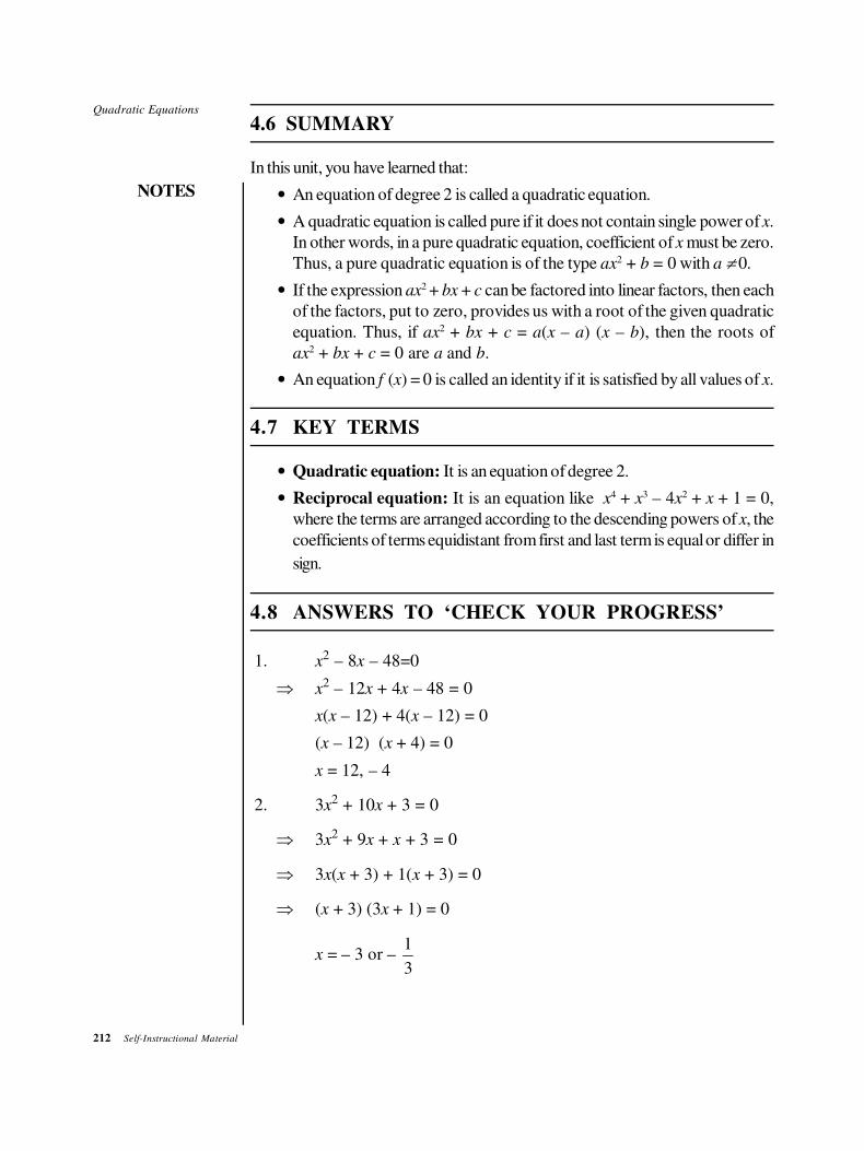
212 Self-Instructional Material
Quadratic Equations
NOTES
4.6 SUMMARY
In this unit, you have learned that:
• An equation of degree 2 is called a quadratic equation.
• A quadratic equation is called pure if it does not contain single power of x.
In other words, in a pure quadratic equation, coefficient of x must be zero.
Thus, a pure quadratic equation is of the type ax2 + b = 0 with a ≠ 0.
• If the expression ax2 + bx + c can be factored into linear factors, then each
of the factors, put to zero, provides us with a root of the given quadratic
equation. Thus, if ax2 + bx + c = a(x – a) (x – b), then the roots of
ax2 + bx + c = 0 are a and b.
• An equation f (x) = 0 is called an identity if it is satisfied by all values of x.
4.7 KEY TERMS
• Quadratic equation: It is an equation of degree 2.
• Reciprocal equation: It is an equation like x4 + x3 – 4x2 + x + 1 = 0,
where the terms are arranged according to the descending powers of x, the
coefficients of terms equidistant from first and last term is equal or differ in
sign.
4.8 ANSWERS TO ‘CHECK YOUR PROGRESS’
1. x2 – 8x – 48=0
⇒ x2 – 12x + 4x – 48 = 0
x(x – 12) + 4(x – 12) = 0
(x – 12) (x + 4) = 0
x = 12, – 4
2. 3x2 + 10x + 3 = 0
⇒ 3x2 + 9x + x + 3 = 0
⇒ 3x(x + 3) + 1(x + 3) = 0
⇒ (x + 3) (3x + 1) = 0
x = – 3 or – 1
3
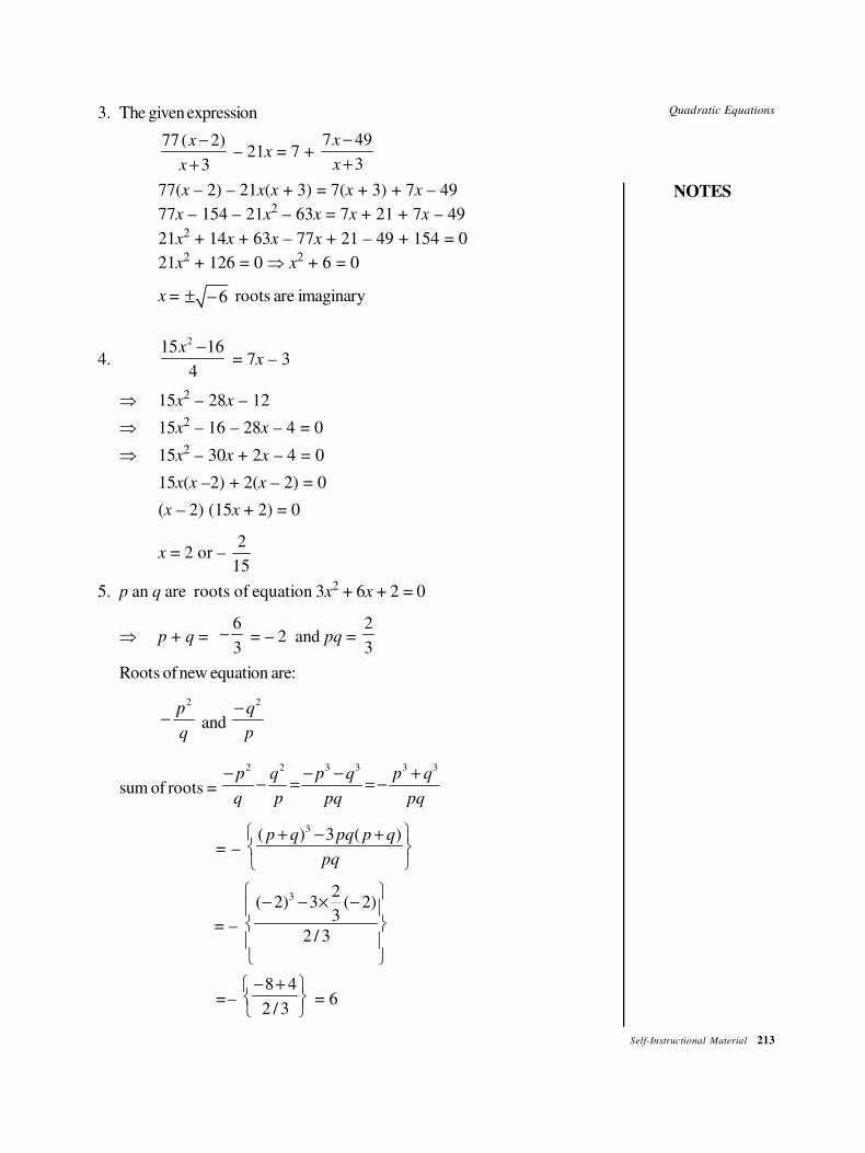
Quadratic Equations
NOTES
Self-Instructional Material 213
3. The given expression
77( 2)
3
x
x
−
+ – 21x = 7 +
7 49
3
x
x
−
+
77(x – 2) – 21x(x + 3) = 7(x + 3) + 7x – 49
77x – 154 – 21x2 – 63x = 7x + 21 + 7x – 49
21x2 + 14x + 63x – 77x + 21 – 49 + 154 = 0
21x2 + 126 = 0 ⇒ x2 + 6 = 0
x = 6± − roots are imaginary
4.
215 16
4
x − = 7x – 3
⇒ 15x2 – 28x – 12
⇒ 15x2 – 16 – 28x – 4 = 0
⇒ 15x2 – 30x + 2x – 4 = 0
15x(x –2) + 2(x – 2) = 0
(x – 2) (15x + 2) = 0
x = 2 or – 2
15
5. p an q are roots of equation 3x2 + 6x + 2 = 0
⇒ p + q = 6
3− = – 2 and pq =
2
3
Roots of new equation are:
2p
q− and
2q
p
−
sum of roots =
2 2 3 3 3 3p q p q p q
q p pq pq
− − − +− = = −
= –
3( ) 3 ( )p q pq p q
pq
+ − +
= –
3 2( 2) 3 ( 2)
3
2 / 3
− − × −
=– 8 4
2 / 3
− +
= 6
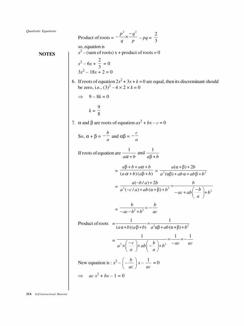
214 Self-Instructional Material
Quadratic Equations
NOTES
Product of roots =
2 2p q
q p
−− × – pq =
2
3
so, equation is
x2 – (sum of roots) x + product of roots = 0
x2 – 6x +
2
3 = 0
3x2 – 18x + 2 = 0
6. If roots of equation 2x2 + 3x + k = 0 are equal, then its discreminant should
be zero, i.e., (3)2 – 4 × 2 × k = 0
⇒ 9 – 8k = 0
k = 9
8
7. α and β are roots of equation ax2 + bx – c = 0
So, α + β = b
a− and αβ =
c
a−
If roots of equation are 1 1
andβ +a b a bα +
= β
( ) ( β )
a b a b
a b a b
α
α
+ + +
+ + = 2 2
(α β) 2
(αβ) α β
a b
a ab ab b
+ +
+ + +
= 2 22
( / ) 2
( / ) (α β)
a b a b b
ba c a ab bac ab b
a
− +=
−− + + + − + +
= 2 2
b b
ac b b ac= −
− − +
Product of roots =2 2
1 1
( α ) ( β ) αβ (α+β)a b a b a ab b=
+ + + +
= 2 2
1 1 1
c b ac aca ab b
a a
= = −− −
× + − +
New equation is : x2 – b
ac
−
x – 1
ac = 0
⇒ ac x2 + bx – 1 = 0
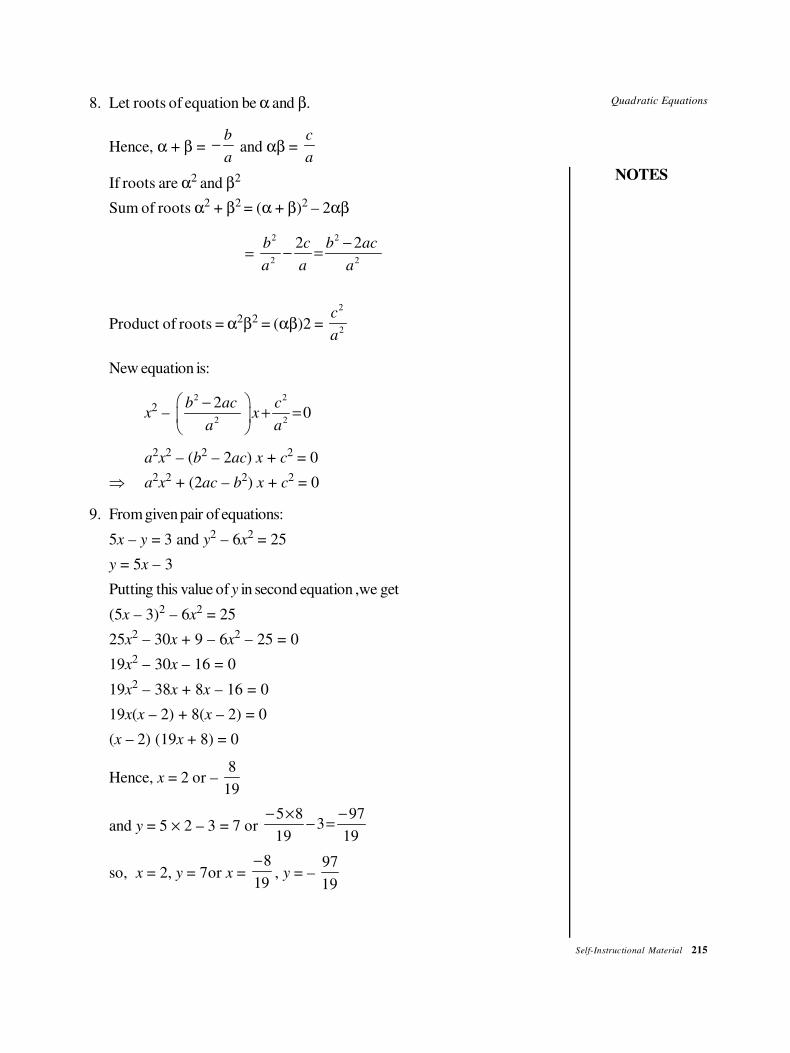
Quadratic Equations
NOTES
Self-Instructional Material 215
8. Let roots of equation be α and β.
Hence, α + β = b
a− and αβ =
c
a
If roots are α2 and β2
Sum of roots α2 + β2 = (α + β)2 – 2αβ
= 2 2
2 2
2 2b c b ac
a a a
−− =
Product of roots = α2β2 = (αβ)2 =
2
2
c
a
New equation is:
x2 –
2 2
2 2
20
b ac cx
a a
−+ =
a2x
2 – (b2 – 2ac) x + c2 = 0
⇒ a2x
2 + (2ac – b2) x + c2 = 0
9. From given pair of equations:
5x – y = 3 and y2 – 6x2 = 25
y = 5x – 3
Putting this value of y in second equation ,we get
(5x – 3)2 – 6x2 = 25
25x2 – 30x + 9 – 6x
2 – 25 = 0
19x2 – 30x – 16 = 0
19x2 – 38x + 8x – 16 = 0
19x(x – 2) + 8(x – 2) = 0
(x – 2) (19x + 8) = 0
Hence, x = 2 or – 8
19
and y = 5 × 2 – 3 = 7 or 5 8 97
319 19
− × −− =
so, x = 2, y = 7or x = 8
19
−, y = –
97
19
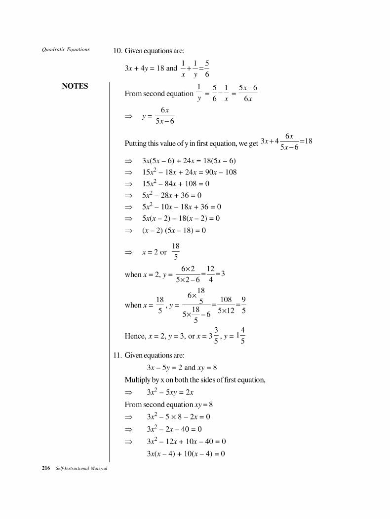
216 Self-Instructional Material
Quadratic Equations
NOTES
10. Given equations are:
3x + 4y = 18 and 1 1 5
6x y+ =
From second equation 1
y =
5 1
6 x− =
5 6
6
x
x
−
⇒ y = 6
5 6
x
x −
Putting this value of y in first equation, we get 6
3 4 185 6
xx
x+ =
−
⇒ 3x(5x – 6) + 24x = 18(5x – 6)
⇒ 15x2 – 18x + 24x = 90x – 108
⇒ 15x2 – 84x + 108 = 0
⇒ 5x2 – 28x + 36 = 0
⇒ 5x2 – 10x – 18x + 36 = 0
⇒ 5x(x – 2) – 18(x – 2) = 0
⇒ (x – 2) (5x – 18) = 0
⇒ x = 2 or 18
5
when x = 2, y = 6 2 12
35 2 – 6 4
×= =
×
when x = 18
5, y =
186
108 9518 5 12 5
5 – 65
×= =
××
Hence, x = 2, y = 3, or x = 33
5, y =
41
5
11. Given equations are:
3x – 5y = 2 and xy = 8
Multiply by x on both the sides of first equation,
⇒ 3x2 – 5xy = 2x
From second equation xy = 8
⇒ 3x2 – 5 × 8 – 2x = 0
⇒ 3x2 – 2x – 40 = 0
⇒ 3x2 – 12x + 10x – 40 = 0
3x(x – 4) + 10(x – 4) = 0
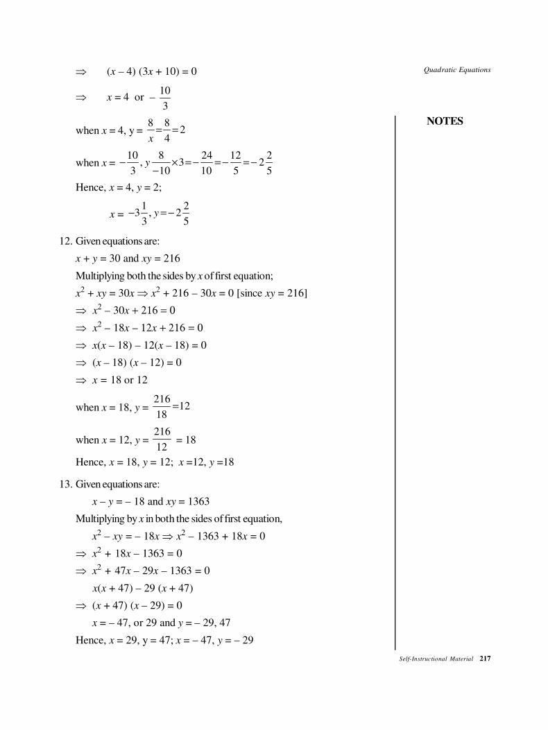
Quadratic Equations
NOTES
Self-Instructional Material 217
⇒ (x – 4) (3x + 10) = 0
⇒ x = 4 or – 10
3
when x = 4, y = 8 8
24x
= =
when x = 10 8 24 12 2
, 3 23 10 10 5 5
y− × = − = − = −−
Hence, x = 4, y = 2;
x = 1 2
3 , 23 5
y− = −
12. Given equations are:
x + y = 30 and xy = 216
Multiplying both the sides by x of first equation;
x2 + xy = 30x ⇒ x2 + 216 – 30x = 0 [since xy = 216]
⇒ x2 – 30x + 216 = 0
⇒ x2 – 18x – 12x + 216 = 0
⇒ x(x – 18) – 12(x – 18) = 0
⇒ (x – 18) (x – 12) = 0
⇒ x = 18 or 12
when x = 18, y = 216
1218
=
when x = 12, y = 216
12 = 18
Hence, x = 18, y = 12; x =12, y =18
13. Given equations are:
x – y = – 18 and xy = 1363
Multiplying by x in both the sides of first equation,
x2 – xy = – 18x ⇒ x2 – 1363 + 18x = 0
⇒ x2 + 18x – 1363 = 0
⇒ x2 + 47x – 29x – 1363 = 0
x(x + 47) – 29 (x + 47)
⇒ (x + 47) (x – 29) = 0
x = – 47, or 29 and y = – 29, 47
Hence, x = 29, y = 47; x = – 47, y = – 29
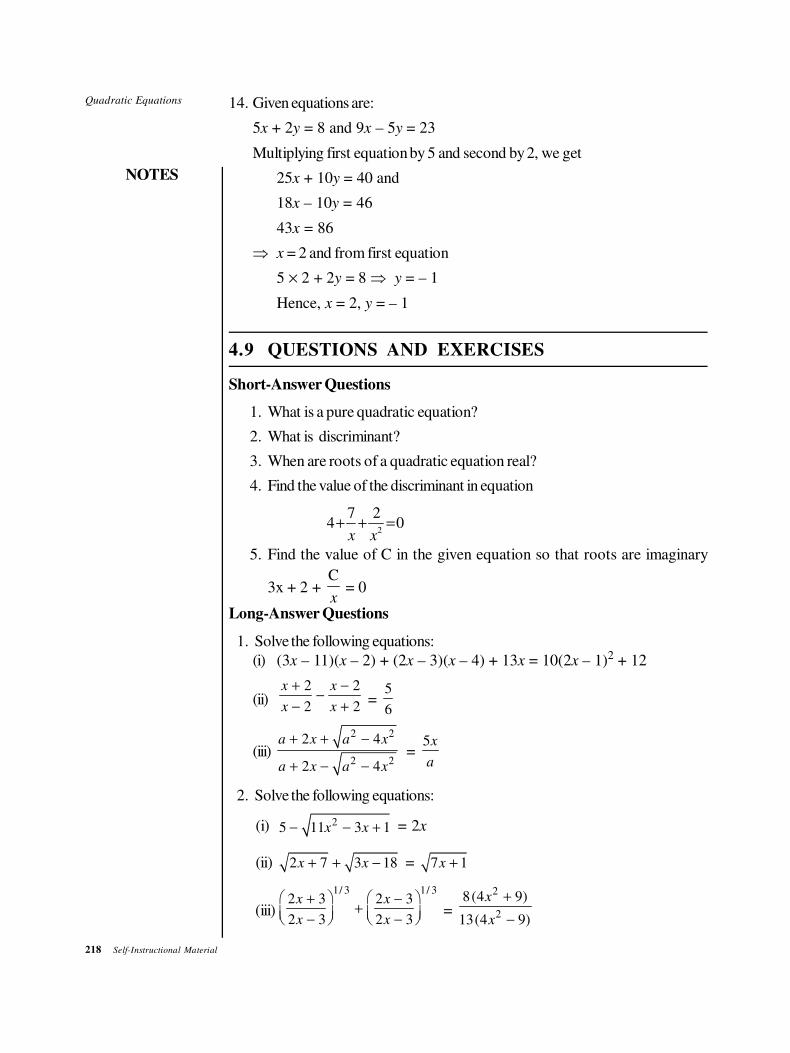
218 Self-Instructional Material
Quadratic Equations
NOTES
14. Given equations are:
5x + 2y = 8 and 9x – 5y = 23
Multiplying first equation by 5 and second by 2, we get
25x + 10y = 40 and
18x – 10y = 46
43x = 86
⇒ x = 2 and from first equation
5 × 2 + 2y = 8 ⇒ y = – 1
Hence, x = 2, y = – 1
4.9 QUESTIONS AND EXERCISES
Short-Answer Questions
1. What is a pure quadratic equation?
2. What is discriminant?
3. When are roots of a quadratic equation real?
4. Find the value of the discriminant in equation
2
7 24 0
x x+ + =
5. Find the value of C in the given equation so that roots are imaginary
3x + 2 + C
x = 0
Long-Answer Questions
1. Solve the following equations:
0 (i) (3x – 11)(x – 2) + (2x – 3)(x – 4) + 13x = 10(2x – 1)2 + 12
0 (ii)2 2
2 2
x x
x x
+ −−
− + = 5
6
(iii)
2 2
2 2
2 4
2 4
a x a x
a x a x
+ + −
+ − − =
5x
a
2. Solve the following equations:
0 (i) 25 11 3 1x x− − + = 2x
(ii) 2 7 3 18x x+ + − = 7 1x +
(iii)
1/ 3 1/ 32 3 2 3
2 3 2 3
x x
x x
+ −+ − −
=
2
2
8(4 9)
13(4 9)
x
x
+
−
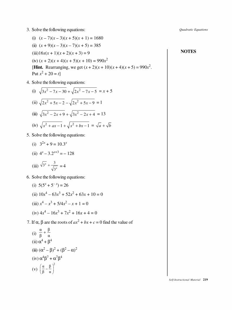
Quadratic Equations
NOTES
Self-Instructional Material 219
3. Solve the following equations:
(i) (x – 7)(x – 3)(x + 5)(x + 1) = 1680
(ii) (x + 9)(x – 3)(x – 7)(x + 5) = 385
(iii)16x(x + 1)(x + 2)(x + 3) = 9
(iv) (x + 2)(x + 4)(x + 5)(x + 10) = 990x2
[Hint. Rearranging, we get (x + 2)(x + 10)(x + 4)(x + 5) = 990x2.
Put x2 + 20 = t]
4. Solve the following equations:
(i) 2 23 7 30 2 7 5x x x x− − + − − = x + 5
(ii) 2 22 5 2 2 5 9x x x x+ − − + − = 1
(iii) 2 23 2 9 3 2 4x x x x− + + − + = 13
(iv) 2 21 1x ax x bx+ − + + − = a b+
5. Solve the following equations:
(i) 32x + 9 = 10.3x
(ii) 4x – 3.2x+3 = – 128
(iii) 3
33
x
x+ = 4
6. Solve the following equations:
(i) 5(5x + 5– x) = 26
(ii) 10x4 – 63x
3 + 52x2 + 63x + 10 = 0
(iii) x4 – x3 + 5/4x2 – x + 1 = 0
(iv) 4x4 – 16x
3 + 7x2 + 16x + 4 = 0
7. If α, β are the roots of ax2 + bx + c = 0 find the value of
(i) α β
β α+ 0
(ii) α4 + β40
(iii) (α2 – β)2 + (β2 – α)2
(iv) α4β7 + α7β40
(v)
2α β
–β α
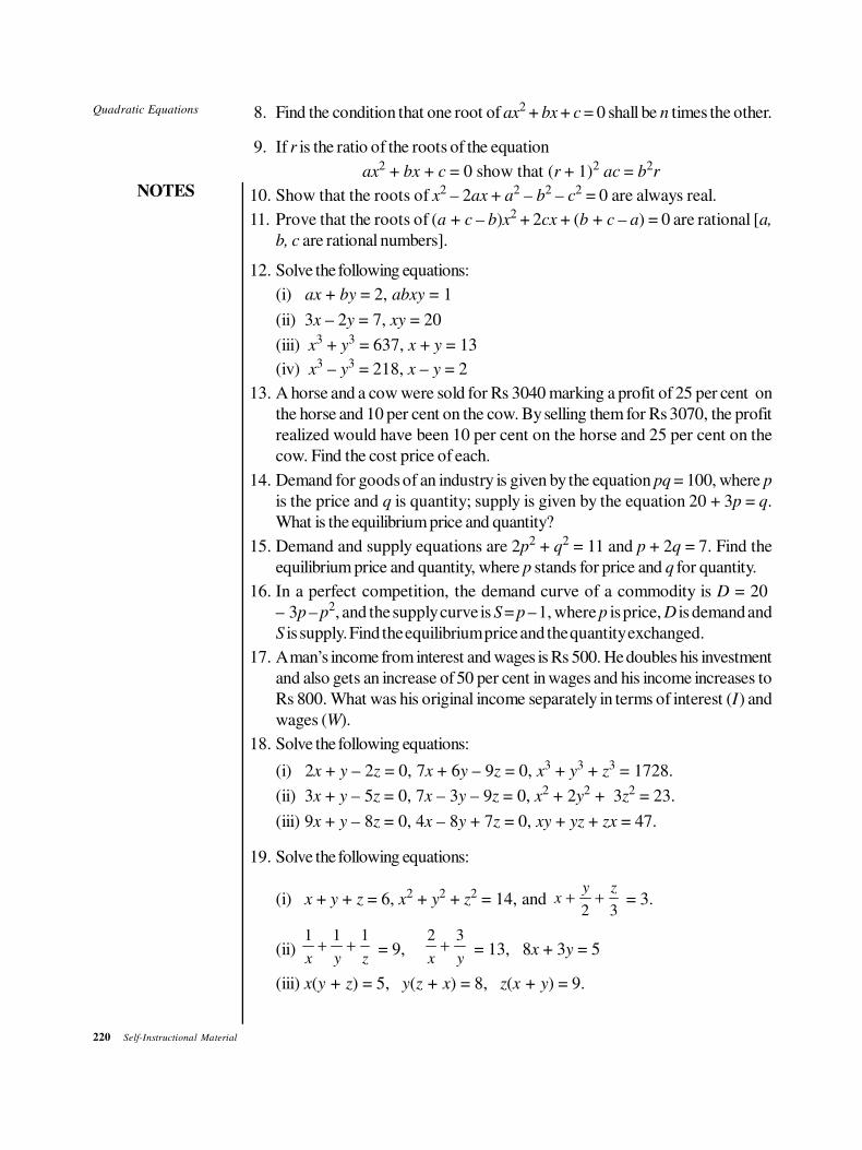
220 Self-Instructional Material
Quadratic Equations
NOTES
8. Find the condition that one root of ax2 + bx + c = 0 shall be n times the other.
9. If r is the ratio of the roots of the equation
ax2 + bx + c = 0 show that (r + 1)2 ac = b2
r
10. Show that the roots of x2 – 2ax + a2 – b2 – c2 = 0 are always real.
11. Prove that the roots of (a + c – b)x2 + 2cx + (b + c – a) = 0 are rational [a,
b, c are rational numbers].
12. Solve the following equations:
(i) ax + by = 2, abxy = 1
(ii) 3x – 2y = 7, xy = 20
(iii) x3 + y3 = 637, x + y = 13
(iv) x3 – y3 = 218, x – y = 2
13. A horse and a cow were sold for Rs 3040 marking a profit of 25 per cent on
the horse and 10 per cent on the cow. By selling them for Rs 3070, the profit
realized would have been 10 per cent on the horse and 25 per cent on the
cow. Find the cost price of each.
14. Demand for goods of an industry is given by the equation pq = 100, where p
is the price and q is quantity; supply is given by the equation 20 + 3p = q.
What is the equilibrium price and quantity?
15. Demand and supply equations are 2p2 + q2 = 11 and p + 2q = 7. Find the
equilibrium price and quantity, where p stands for price and q for quantity.
16. In a perfect competition, the demand curve of a commodity is D = 20
– 3p – p2, and the supply curve is S = p – 1, where p is price, D is demand and
S is supply. Find the equilibrium price and the quantity exchanged.
17. A man’s income from interest and wages is Rs 500. He doubles his investment
and also gets an increase of 50 per cent in wages and his income increases to
Rs 800. What was his original income separately in terms of interest (I) and
wages (W).
18. Solve the following equations:
(i) 2x + y – 2z = 0, 7x + 6y – 9z = 0, x3 + y3 + z3 = 1728.
(ii) 3x + y – 5z = 0, 7x – 3y – 9z = 0, x2 + 2y2 + 3z
2 = 23.
(iii) 9x + y – 8z = 0, 4x – 8y + 7z = 0, xy + yz + zx = 47.
19. Solve the following equations:
(i) x + y + z = 6, x2 + y2 + z2 = 14, and 2 3
y zx + + = 3.
(ii) 1 1 1
x y z+ + = 9,
2 3
x y+ = 13, 8x + 3y = 5
(iii) x(y + z) = 5, y(z + x) = 8, z(x + y) = 9.
Quadratic Equations
NOTES
Self-Instructional Material 221
4.10 FURTHER READING
Khanna, V.K, S.K. Bhambri, C.B. Gupta and Vijay Gupta. Quantitative
Techniques. New Delhi: Vikas Publishing House.
Khanna, V.K, S.K. Bhambri and Quazi Zameeruddin. Business Mathematics.
New Delhi:Vikas Publishing House.

Complex Numbers
NOTES
Self-Instructional Material 223
UNIT 5 COMPLEX NUMBERS
Structure
5.0 Introduction
5.1 Unit Objectives
5.2 Imaginary Numbers
5.2.1 Definition of Complex Number
5.3 Complex Numbers: Basic Characteristics
5.3.1 Geometric Representation of Complex Numbers
5.3.2 Complex Arithmetic
5.3.3 Operations on Complex Numbers
5.3.4 Graphical Representation
5.3.5 Quadratic Functions and their Graphs
5.3.6 Polynomial Functions and their Graphs
5.3.7 Division of Univariate Polynomials
5.3.8 Zeros of Polynomial Functions
5.3.9 Rational Functions and their Graphs
5.3.10 Polynomial and Rational Inequalities
5.4 Uses of Complex Numbers
5.4.1 History of Complex Numbers
5.4.2 Geometrical Representation of Conjugates
5.4.3 Geometric Interpretation of Addition and Multiplication Operations
5.4.4 Matrix Representation of Complex Numbers
5.5 Properties of Complex Numbers
5.5.1 Applications of Complex Numbers
5.5.2 Signal Analysis
5.6 Summary
5.7 Key Terms
5.8 Answers to ‘Check Your Progress’
5.9 Questions and Exercises
5.10 Further Reading
5.0 INTRODUCTION
We all are familiar with real numbers and use it in our number system. There is also
another important class of numbers termed as complex numbers, which consists
of imaginary as well as real numbers. In spite of the term imaginary, these numbers
are exceptionally used in various areas of science, such as electromagnetic theory,
relativity and quantum mechanics.
Girolamo Cardano was an Italian mathematician who first realized the need
of finding complex numbers. While solving cubic equations he came across
expressions that contained square root of a negative number. Thus, the concept of
an imaginary number took birth but this was accepted as a part of mathematical
concept by the work of Abraham De Moivre, Bernoullis and Leonhard Euler,
who carried out studies on this topic in detail. De Moivre was a French-English
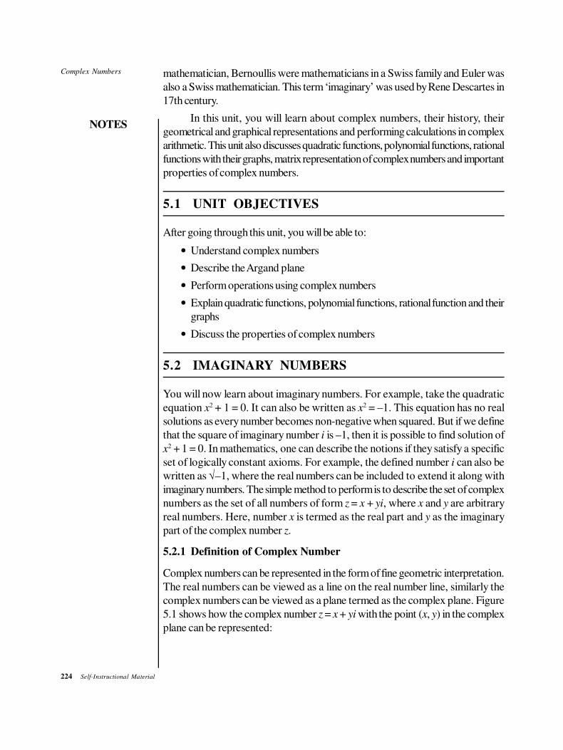
224 Self-Instructional Material
Complex Numbers
NOTES
mathematician, Bernoullis were mathematicians in a Swiss family and Euler was
also a Swiss mathematician. This term ‘imaginary’ was used by Rene Descartes in
17th century.
In this unit, you will learn about complex numbers, their history, their
geometrical and graphical representations and performing calculations in complex
arithmetic. This unit also discusses quadratic functions, polynomial functions, rational
functions with their graphs, matrix representation of complex numbers and important
properties of complex numbers.
5.1 UNIT OBJECTIVES
After going through this unit, you will be able to:
• Understand complex numbers
• Describe the Argand plane
• Perform operations using complex numbers
• Explain quadratic functions, polynomial functions, rational function and their
graphs
• Discuss the properties of complex numbers
5.2 IMAGINARY NUMBERS
You will now learn about imaginary numbers. For example, take the quadratic
equation x2 + 1 = 0. It can also be written as x2 = –1. This equation has no real
solutions as every number becomes non-negative when squared. But if we define
that the square of imaginary number i is –1, then it is possible to find solution of
x2 + 1 = 0. In mathematics, one can describe the notions if they satisfy a specific
set of logically constant axioms. For example, the defined number i can also be
written as √–1, where the real numbers can be included to extend it along with
imaginary numbers. The simple method to perform is to describe the set of complex
numbers as the set of all numbers of form z = x + yi, where x and y are arbitrary
real numbers. Here, number x is termed as the real part and y as the imaginary
part of the complex number z.
5.2.1 Definition of Complex Number
Complex numbers can be represented in the form of fine geometric interpretation.
The real numbers can be viewed as a line on the real number line, similarly the
complex numbers can be viewed as a plane termed as the complex plane. Figure
5.1 shows how the complex number z = x + yi with the point (x, y) in the complex
plane can be represented:
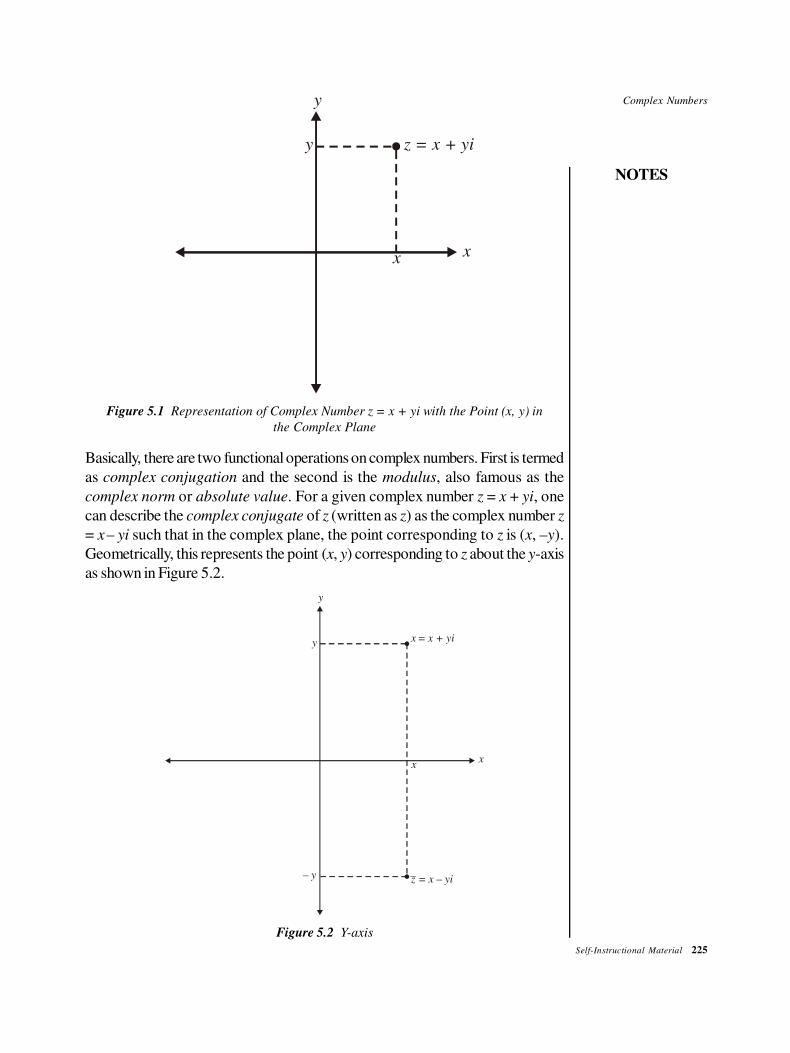
Complex Numbers
NOTES
Self-Instructional Material 225
y
y
xx
z = x + yi
Figure 5.1 Representation of Complex Number z = x + yi with the Point (x, y) in
the Complex Plane
Basically, there are two functional operations on complex numbers. First is termed
as complex conjugation and the second is the modulus, also famous as the
complex norm or absolute value. For a given complex number z = x + yi, one
can describe the complex conjugate of z (written as z) as the complex number z
= x – yi such that in the complex plane, the point corresponding to z is (x, –y).
Geometrically, this represents the point (x, y) corresponding to z about the y-axis
as shown in Figure 5.2.
x x + yi = y
y
xx
– yz = x – yi
Figure 5.2 Y-axis
226 Self-Instructional Material
Complex Numbers
NOTES
In case of modulus, a given complex number z = x + yi denotes its modulus as |z|
and is given by the following formula:
|z| = √x2 + y2
As per the distance formula it is equal to the distance from the origin O =
(0, 0) up to the point P = (x, y). Hence, the complex number is considered as the
length of the line segment passing through the origin to the point in a complex
plane.
Rule for Zero: A complex number is equal to zero only when its real part and its
imaginary part are equal to zero. For example, a + bi = 0 if and only if a = 0 and
b = 0. Similarly, the complex numbers are equal if their real and imaginary parts
are equal.
CHECK YOUR PROGRESS
1. How can the quadratic equation x2 + 1 = 0 also be written as?
2. What is the rule for zero?
5.3 COMPLEX NUMBERS: BASIC
CHARACTERISTICS
A complex number has two parts, real and imaginary. A number is imaginary when
it is the square root of a negative real number. For example, if x2 = 1, then x = ±
√1 = ± 1. Such a square root has both real values. But if there is an equation
x2 + 1 = 0 → x2 = – 1 and hence, x = √–1 and this number is imaginary since there
is no real number that satisfies this condition then this number, given by √–1 is an
imaginary number and it is designated by using letter i.
A number with an expression containing two terms is known as binomial.
Thus, a complex number has two terms in which one is real and the other is
imaginary and is multiple of i. A complex number is symbolically expressed in the
form of a + bi or x + yi, where a, b, x and y are real numbers, and i is an imaginary
number given as i = √–1. This means that i2 = –1. Following are the complex
numbers:
4 + i, 2 – 5i, 0.5 + 3i and –7 – 3i
In a complex number, these two parts cannot be added or subtracted the way it is
done in case when all are real numbers.
The powers of i have repetition in a cycle:
...
i–3 = i
i–2 = –1
i–1 = –i
i0 = 1
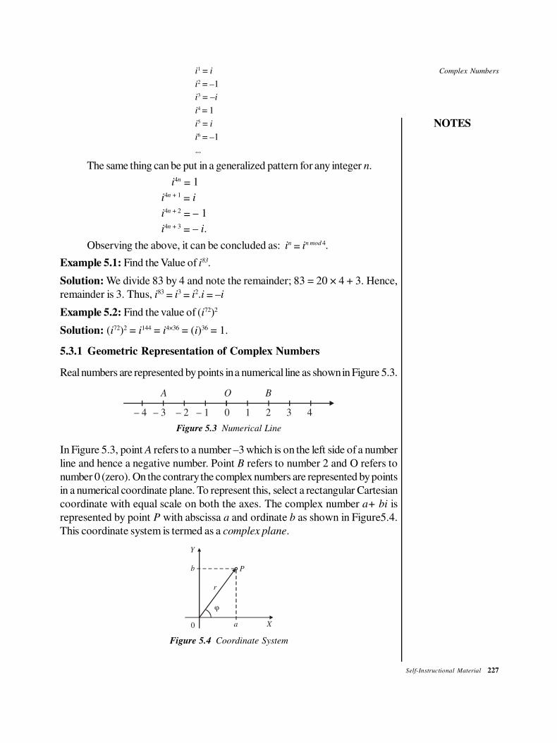
Complex Numbers
NOTES
Self-Instructional Material 227
i1 = i
i2 = –1
i3 = –i
i4 = 1
i5 = i
i6 = –1
...
The same thing can be put in a generalized pattern for any integer n.
i4n = 1
i4n + 1 = i
i4n + 2 = – 1
i4n + 3 = – i.
Observing the above, it can be concluded as: in = in mod 4.
Example 5.1: Find the Value of i83.
Solution: We divide 83 by 4 and note the remainder; 83 = 20 × 4 + 3. Hence,
remainder is 3. Thus, i83 = i3 = i2.i = –i
Example 5.2: Find the value of (i72)2
Solution: (i72)2 = i144 = i4×36 = (i)36 = 1.
5.3.1 Geometric Representation of Complex Numbers
Real numbers are represented by points in a numerical line as shown in Figure 5.3.
A O B
– 4 – 3 – 2 – 1 0 1 2 3 4
Figure 5.3 Numerical Line
In Figure 5.3, point A refers to a number –3 which is on the left side of a number
line and hence a negative number. Point B refers to number 2 and O refers to
number 0 (zero). On the contrary the complex numbers are represented by points
in a numerical coordinate plane. To represent this, select a rectangular Cartesian
coordinate with equal scale on both the axes. The complex number a+ bi is
represented by point P with abscissa a and ordinate b as shown in Figure5.4.
This coordinate system is termed as a complex plane.
Y
P
X
r
a
b
0
Figure 5.4 Coordinate System
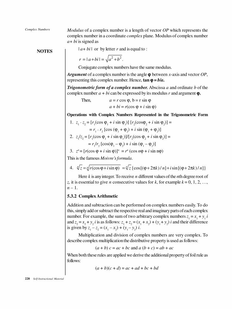
228 Self-Instructional Material
Complex Numbers
NOTES
Modulus of a complex number is a length of vector OP which represents the
complex number in a coordinate complex plane. Modulus of complex number
a+ bi is signed as
| a+ bi | or by letter r and is equal to :
2 2| | .r a bi a b= + = +
Conjugate complex numbers have the same modulus.
Argument of a complex number is the angle ϕϕϕϕ between x-axis and vector OP,
representing this complex number. Hence, tan ϕϕϕϕ = b/a.
Trigonometric form of a complex number. Abscissa a and ordinate b of the
complex number a + bi can be expressed by its modulus r and argument ϕϕϕϕ.
Then, a = r cos ϕ, b = r sin ϕ
a + bi = r(cos ϕ + i sin ϕ)
Operations with Complex Numbers Represented in the Trigonometric Form
1. z1 . z
2 = [r
1(cos ϕ
1 + i sin ϕ
1)] [r
2(cosϕ
2 + i sin ϕ
2)] =
= r1 . r
2 [cos (ϕ
1 + ϕ
2) + i sin (ϕ
1 + ϕ
2)]
2. z1/z
2 = [r
1(cos ϕ
1 + i sin ϕ
1)]/[r
2(cos ϕ
2 + i sin ϕ
2)] =
= r1/r
2 [cos(ϕ
1 – ϕ
2) + i sin (ϕ
1 – ϕ
2)]
3. zn = [r(cos ϕ + i sin ϕ)]n = rn (cos nϕ + i sin nϕ)
This is the famous Moivre’s formula.
4. (cos sin ) {cos[( 2 ) / ] sin[( 2 ) / ]}n nnz r i z k n i k n= ϕ+ ϕ = ϕ+ π + ϕ+ π
Here k is any integer. To receive n different values of the nth degree root of
z, it is essential to give n consecutive values for k, for example k = 0, 1, 2, …,
n – 1.
5.3.2 Complex Arithmetic
Addition and subtraction can be performed on complex numbers easily. To do
this, simply add or subtract the respective real and imaginary parts of each complex
number. For example, the sum of two arbitrary complex numbers z1 = x
1 + y
1 i
and z2 = x
2 + y
2 i is as follows: z
1 + z
2 = (x
1 + x
2) + (y
1 + y
2) i and their difference
is given by z1 – z
2 = (x
1 – x
2) + (y
1 – y
2) i.
Multiplication and division of complex numbers are very complex. To
describe complex multiplication the distributive property is used as follows:
(a + b) c = ac + bc and a (b + c) = ab + ac
When both these rules are applied we derive the additional property of foil rule as
follows:
(a + b)(c + d) = ac + ad + bc + bd
Complex Numbers
NOTES
Self-Instructional Material 229
Apply the foil rule for computing the product of the above given complex numbers
z1 and z
2. If a = x
1, b = y
1 i, c = x
2, and d = y
2 i, then z
1 z
2 = (x
1 + y
1 i)(x
2 + y
2
i) = x1 x
2 + x
1 y
2 i + y
1 x
2 i + y
1 y
2 i2. If i2 = –1, then z
1 z
2 = (x
1 x
2 – y
1 y
2) +
(x1 y
2 + y
1 x
2) i.
Using this formula any two complex numbers can be multiplied. The following
identity is verified using the above derived complex number definition:
| | .z zz=
Hence, the complex number is equal to the square root of the product of the
number and its complex conjugate. This definition is also used to describe complex
division. Division on complex numbers is very complex. For example, let the
quotients are z1/z
2, where z
1 and z
2 are arbitrary complex numbers and z
2 is nonzero.
When the numerator and denominator is multiplied by the complex conjugate of
z2, then the result is (z
1/z
2)(z
2/z
2) = z
1z
2 / |z
2|2.
To divide two complex numbers in terms of the real and imaginary parts of z1 and
z2 is shown below:
1 1 1 1 2 1 2 2 1 1 22 2
2 2 2 2 2
( ) ( )z x y i x x y y x y x y i
z x y i x y
+ + + −= =
+ +
Operations on complex numbers are like those on real numbers in many ways.
But there are two exceptions of these rules. Two exceptions to this are:
1. Addition of subtraction of the two terms of a complex number a + bi can
not be done and should be left as it is.
2. An expression i2 = –1, is against the general rule that product of two numbers
having same sign is positive. If we take i.i = i2 = –1. If we take it like i.i =
√–1.√–1 = √(–1)(–1) = √1 = 1. Two results are contradictory.
5.3.3 Operations on Complex Numbers
The following are the general rules for operations on complex numbers:
1. Equality: Two complex numbers are equal if their real parts and imaginary
parts are each equal. If two complex numbers c1 = x + yi and c2 = w + zi
and c1 = c2, this means x + yi = w + zi and this leads to the fact that x =
w and y = z.
2. Addition: If there are two complex numbers a + bi and c + di and if they
are added together, their real parts are added together and the same applies
to their imaginary parts too. For example,
(a + bi) + (c + di) = (a + c) + (b + d)i
Here, the real part of first is added to the real part of the other and the imaginary
part of one is added to the imaginary part of the other.
230 Self-Instructional Material
Complex Numbers
NOTES
Example 5.3: If z1 =
(2 + 3i) and z
2 = (5 – 9i), find z
1 + z
2.
Solution: z1 + z
2 = (2 + 5) + (3 + (–9))i = 7 – 6i.
3. Subtraction: If one complex number c + di, is subtracted from another
complex number a + bi, then real part c, is subtracted from real part a, and
imaginary part d, is subtracted from the imaginary part b. This is shown as
below:
(a + bi) – (c + di) = (a – c) + (b – d)i
Example 5.4: If If z1 =
(3 + 11i) and z
2 = (7 + 13i), find z
1 − z
2.
Solution: z1 − z
2 = (3 + 11i) − (7 + 13i) = −4 −2i
4. Zero: If a complex number is zero, then both the parts are separately zero.
For example, if x +yi = 0, this means that x = 0 and y = 0.
5. Opposites: To find opposite of a complex number, change the sign of each
part. If a + bi is a complex number, its opposite id found by its negation,
i.e., as –(a + bi) that leads to –a + (–b)i = –a –bi. Opposite of a complex
number 7 – 4i is –7 + 4i.
6. Multiplication: Product of two complex numbers is also a complex number.
If z1 and z
2 are two complex numbers where z
1 =
x
1 + y
1i and z
2 = x
2 + y
2i,
their product z1 × z
2 is given by (x
1 + y
1i) × (x
2 + y
2i) = x
1x
2 + x
1y
2 i +
y
1x
2i
+ y1y
2i2. Since i2 = –1, y
1y
2i2 = –y
1y
2.
Thus, z1 × z
2 = (x
1x
2 –y
1y
2) + (x
1y
2 +
y
1x
2)i and this too is a complex number
having (x1x
2 –y
1y
2)
as its real part and (x
1y
2 +
y
1x
2)
as its imaginary part.
7. Conjugates: Every complex number has conjugate that is found just by
changing the sign of its imaginary part. If x + yi is a complex number its
conjugate is x – yi. Thus, x + yi and x – yi are conjugate pairs known as
complex conjugates. This is denoted by placing a bar over the symbol. If
z = x + yi, is a complex number, its conjugate is denoted as z x yi= − and
z z× is given by x2 + y2. Thus, product of a conjugate pair is always a real
number.
Example 5.5: A complex number is given as z = 7 + 5i. Find its conjugate and
also find the product of the conjugate pair.
Solution: If z = 7 + 5i then its conjugate is given by z = 7 – 5i. Their product
z z× is given by 72 + 52 = 49 + 25 = 77.
8. Division: If a complex number is divided by another complex number, it
gives a complex number. Thus, the result of division of one complex number
by another is also a complex number. If z1 =
x
1 + y
1i and z
2 = x
2 + y
2i are
two complex numbers and z1 is divided by z
2+ then, z
2 can not be zero,
since division by zero is not allowed. Also, complex number in the
denominator side should be converted to a real number to perform this
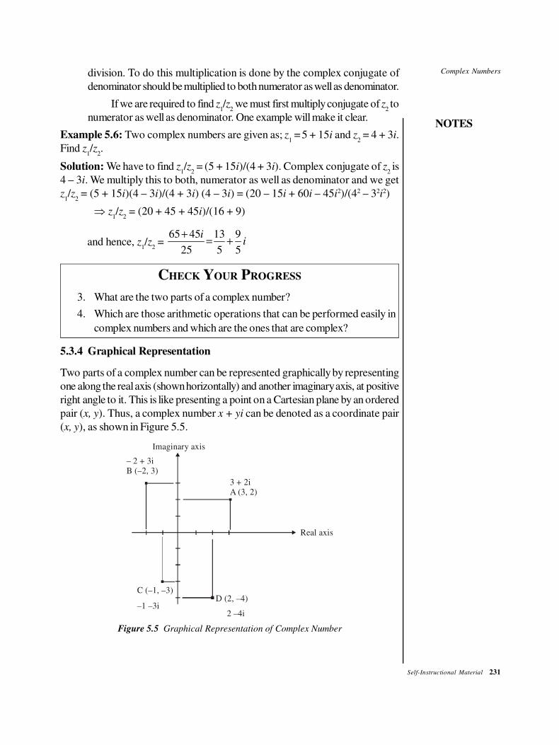
Complex Numbers
NOTES
Self-Instructional Material 231
division. To do this multiplication is done by the complex conjugate of
denominator should be multiplied to both numerator as well as denominator.
If we are required to find z1/z
2 we must first multiply conjugate of z
2 to
numerator as well as denominator. One example will make it clear.
Example 5.6: Two complex numbers are given as; z1 =
5 + 15i and z
2 = 4 + 3i.
Find z1/z
2.
Solution: We have to find z1/z
2 = (5 + 15i)/(4 + 3i). Complex conjugate of z
2 is
4 – 3i. We multiply this to both, numerator as well as denominator and we get
z1/z
2 = (5 + 15i)(4 – 3i)/(4 + 3i) (4 – 3i) = (20 – 15i + 60i – 45i2)/(42 – 32i2)
⇒ z1/z
2 = (20 + 45 + 45i)/(16 + 9)
and hence, z1/z
2 =
65 45 13 9
25 5 5
ii
+= +
CHECK YOUR PROGRESS
3. What are the two parts of a complex number?
4. Which are those arithmetic operations that can be performed easily in
complex numbers and which are the ones that are complex?
5.3.4 Graphical Representation
Two parts of a complex number can be represented graphically by representing
one along the real axis (shown horizontally) and another imaginary axis, at positive
right angle to it. This is like presenting a point on a Cartesian plane by an ordered
pair (x, y). Thus, a complex number x + yi can be denoted as a coordinate pair
(x, y), as shown in Figure 5.5.
Imaginary axis
– 2 + 3iB (–2, 3)
3 + 2iA (3, 2)
Real axis
C (–1, –3)
–1 –3iD (2, –4)
2 –4i
Figure 5.5 Graphical Representation of Complex Number
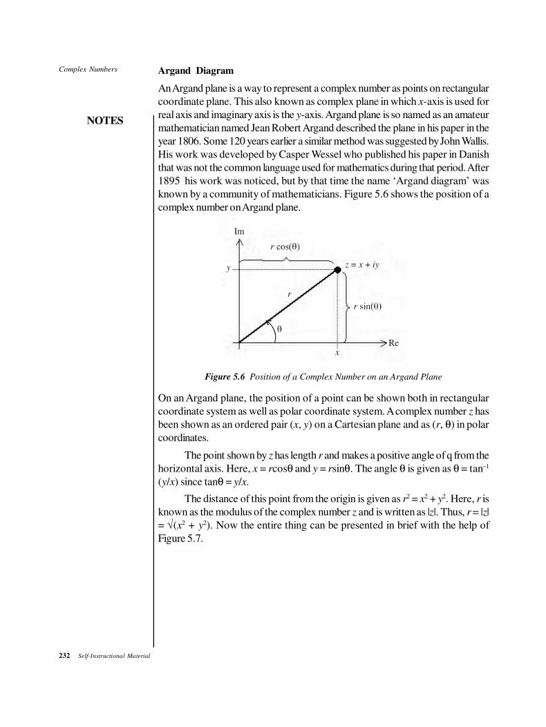
232 Self-Instructional Material
Complex Numbers
NOTES
Argand Diagram
An Argand plane is a way to represent a complex number as points on rectangular
coordinate plane. This also known as complex plane in which x-axis is used for
real axis and imaginary axis is the y-axis. Argand plane is so named as an amateur
mathematician named Jean Robert Argand described the plane in his paper in the
year 1806. Some 120 years earlier a similar method was suggested by John Wallis.
His work was developed by Casper Wessel who published his paper in Danish
that was not the common language used for mathematics during that period. After
1895 his work was noticed, but by that time the name ‘Argand diagram’ was
known by a community of mathematicians. Figure 5.6 shows the position of a
complex number on Argand plane.
Im
y
r
z x iy = +
Rex
Figure 5.6 Position of a Complex Number on an Argand Plane
On an Argand plane, the position of a point can be shown both in rectangular
coordinate system as well as polar coordinate system. A complex number z has
been shown as an ordered pair (x, y) on a Cartesian plane and as (r, θ) in polar
coordinates.
The point shown by z has length r and makes a positive angle of q from the
horizontal axis. Here, x = rcosθ and y = rsinθ. The angle θ is given as θ = tan–1
(y/x) since tanθ = y/x.
The distance of this point from the origin is given as r2 = x2 + y2. Here, r is
known as the modulus of the complex number z and is written as |z|. Thus, r = |z|
= √(x2 + y2). Now the entire thing can be presented in brief with the help of
Figure 5.7.
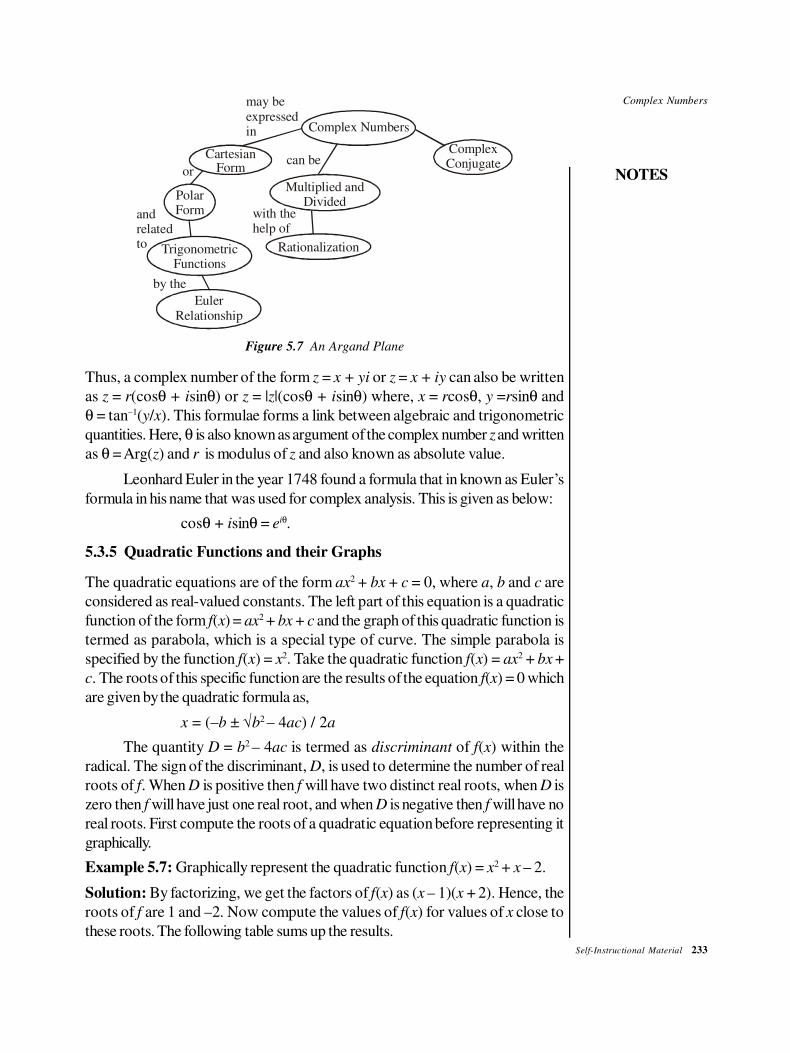
Complex Numbers
NOTES
Self-Instructional Material 233
Complex Numbers
Complex Conjugatecan be
may beexpressedin
or
andrelatedto
by the
with thehelp of
EulerRelationship
TrigonometricFunctions
PolarForm
Multiplied andDivided
CartesianForm
Rationalization
Figure 5.7 An Argand Plane
Thus, a complex number of the form z = x + yi or z = x + iy can also be written
as z = r(cosθ + isinθ) or z = |z|(cosθ + isinθ) where, x = rcosθ, y =rsinθ and
θ = tan–1(y/x). This formulae forms a link between algebraic and trigonometric
quantities. Here, θ is also known as argument of the complex number z and written
as θ = Arg(z) and r is modulus of z and also known as absolute value.
Leonhard Euler in the year 1748 found a formula that in known as Euler’s
formula in his name that was used for complex analysis. This is given as below:
cosθ + isinθ = eiθ.
5.3.5 Quadratic Functions and their Graphs
The quadratic equations are of the form ax2 + bx + c = 0, where a, b and c are
considered as real-valued constants. The left part of this equation is a quadratic
function of the form f(x) = ax2 + bx + c and the graph of this quadratic function is
termed as parabola, which is a special type of curve. The simple parabola is
specified by the function f(x) = x2. Take the quadratic function f(x) = ax2 + bx +
c. The roots of this specific function are the results of the equation f(x) = 0 which
are given by the quadratic formula as,
x = (–b ± √b2 – 4ac) / 2a
The quantity D = b2 – 4ac is termed as discriminant of f(x) within the
radical. The sign of the discriminant, D, is used to determine the number of real
roots of f. When D is positive then f will have two distinct real roots, when D is
zero then f will have just one real root, and when D is negative then f will have no
real roots. First compute the roots of a quadratic equation before representing it
graphically.
Example 5.7: Graphically represent the quadratic function f(x) = x2 + x – 2.
Solution: By factorizing, we get the factors of f(x) as (x – 1)(x + 2). Hence, the
roots of f are 1 and –2. Now compute the values of f(x) for values of x close to
these roots. The following table sums up the results.
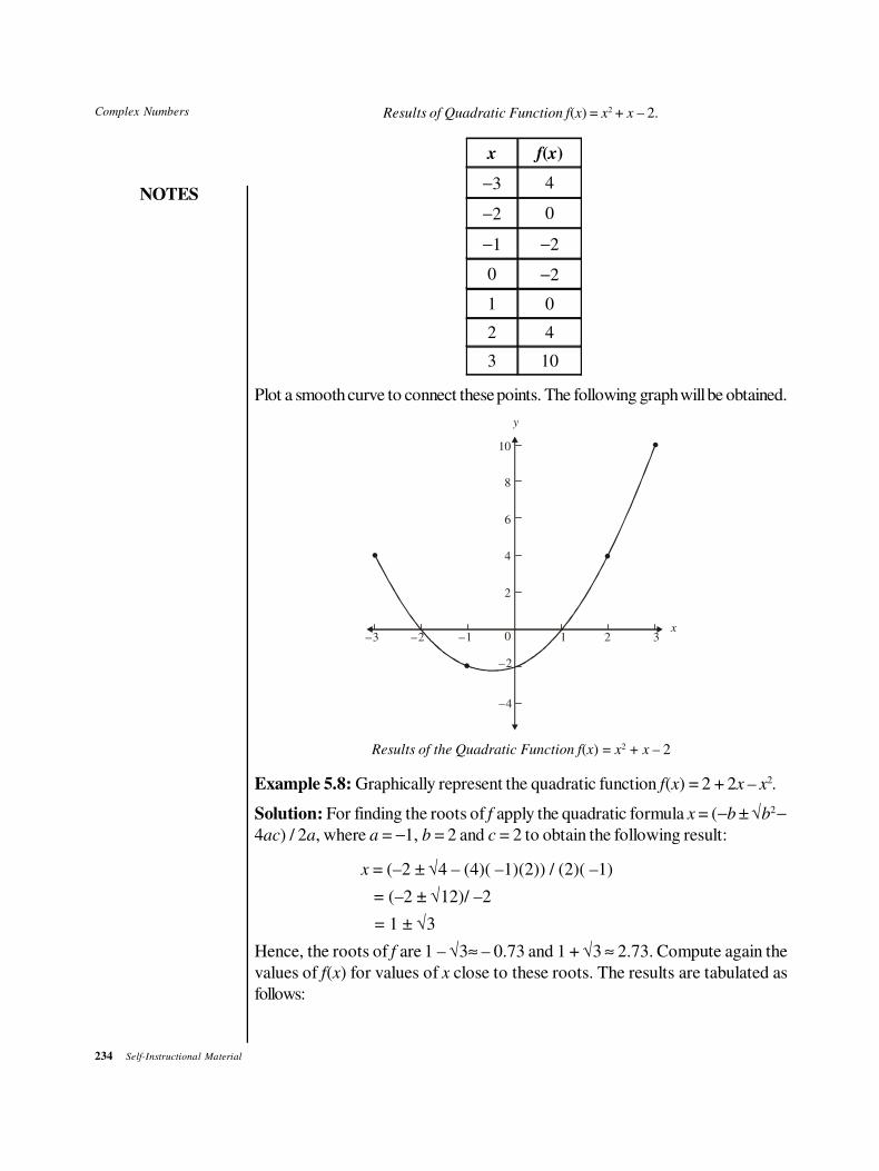
234 Self-Instructional Material
Complex Numbers
NOTES
Results of Quadratic Function f(x) = x2 + x – 2.
x f(x)
−3 4
−2 0
−1 −2
0 −2
1 0
2 4
3 10
Plot a smooth curve to connect these points. The following graph will be obtained.
y
x
10
8
6
4
2
0–3 –2 –1 1 2 3
–2
–4
Results of the Quadratic Function f(x) = x2 + x – 2
Example 5.8: Graphically represent the quadratic function f(x) = 2 + 2x – x2.
Solution: For finding the roots of f apply the quadratic formula x = (−b ± √b2 −4ac) / 2a, where a = −1, b = 2 and c = 2 to obtain the following result:
x = (–2 ± √4 – (4)( –1)(2)) / (2)( –1)
= (–2 ± √12)/ –2
= 1 ± √3
Hence, the roots of f are 1 – √3≈ – 0.73 and 1 + √3 ≈ 2.73. Compute again the
values of f(x) for values of x close to these roots. The results are tabulated as
follows:
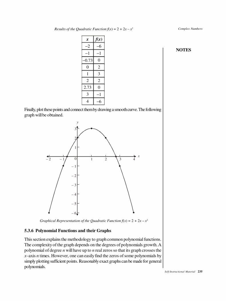
Complex Numbers
NOTES
Self-Instructional Material 235
Results of the Quadratic Function f(x) = 2 + 2x – x2
x f(x)
−2 −6
−1 −1
−0.73 0
0 2
1 3
2 2
2.73 0
3 −1
4 −6
Finally, plot these points and connect them by drawing a smooth curve. The following
graph will be obtained.
y
x
3
2
1
0
– 1
– 2
– 3
– 4
– 5
– 6
– 2 – 1 1 2 3 4
Graphical Representation of the Quadratic Function f(x) = 2 + 2x – x2
5.3.6 Polynomial Functions and their Graphs
This section explains the methodology to graph common polynomial functions.
The complexity of the graph depends on the degrees of polynomials growth. A
polynomial of degree n will have up to n real zeros so that its graph crosses the
x–axis n times. However, one can easily find the zeros of some polynomials by
simply plotting sufficient points. Reasonably exact graphs can be made for general
polynomials.
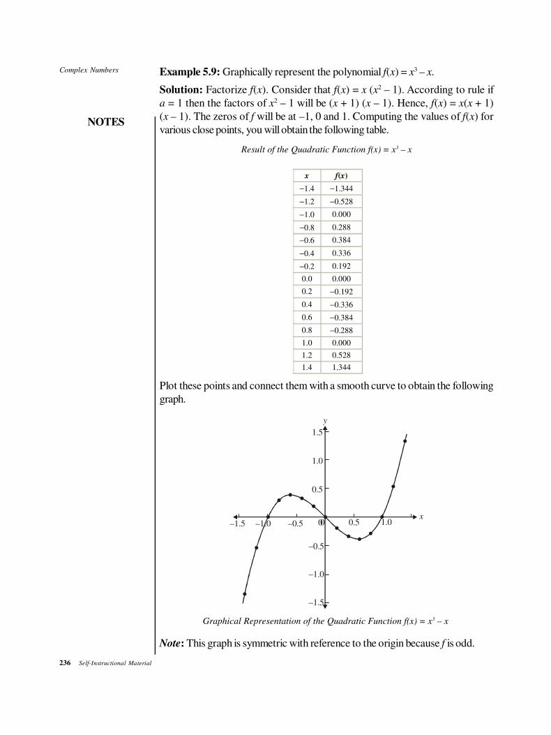
236 Self-Instructional Material
Complex Numbers
NOTES
Example 5.9: Graphically represent the polynomial f(x) = x3 – x.
Solution: Factorize f(x). Consider that f(x) = x (x2 – 1). According to rule if
a = 1 then the factors of x2 – 1 will be (x + 1) (x – 1). Hence, f(x) = x(x + 1)
(x – 1). The zeros of f will be at –1, 0 and 1. Computing the values of f(x) for
various close points, you will obtain the following table.
Result of the Quadratic Function f(x) = x3 – x
x f(x)
−1.4 −1.344
−1.2 −0.528
−1.0 0.000
−0.8 0.288
−0.6 0.384
−0.4 0.336
−0.2 0.192
0.0 0.000
0.2 −0.192
0.4 −0.336
0.6 −0.384
0.8 −0.288
1.0 0.000
1.2 0.528
1.4 1.344
Plot these points and connect them with a smooth curve to obtain the following
graph.
–1.5 –1.0 –0.5 0 0.5 1.0
1.5
1.0
0.5
0
y
x
–0.5
1.0
1.5
–
–
Graphical Representation of the Quadratic Function f(x) = x3 – x
Note: This graph is symmetric with reference to the origin because f is odd.
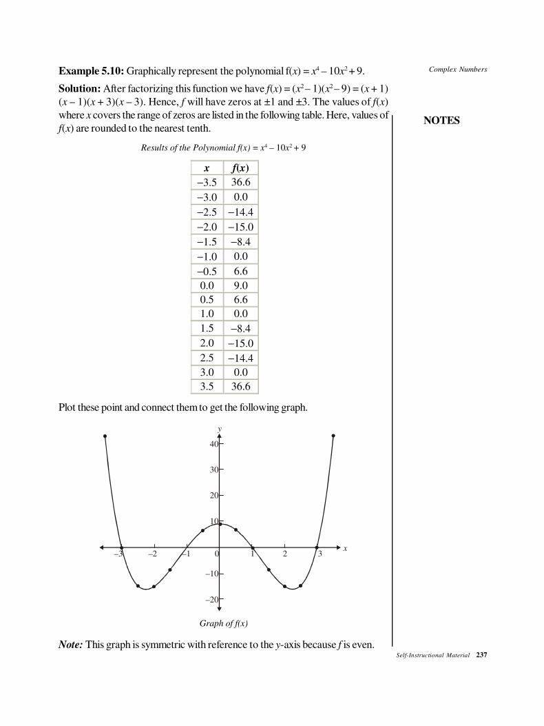
Complex Numbers
NOTES
Self-Instructional Material 237
Example 5.10: Graphically represent the polynomial f(x) = x4 – 10x2 + 9.
Solution: After factorizing this function we have f(x) = (x2 – 1)(x2 – 9) = (x + 1)
(x – 1)(x + 3)(x – 3). Hence, f will have zeros at ±1 and ±3. The values of f(x)
where x covers the range of zeros are listed in the following table. Here, values of
f(x) are rounded to the nearest tenth.
Results of the Polynomial f(x) = x4 – 10x2 + 9
x f(x)
−3.5 36.6
−3.0 0.0
−2.5 −14.4
−2.0 −15.0
−1.5 −8.4
−1.0 0.0
−0.5 6.6
0.0 9.0
0.5 6.6
1.0 0.0
1.5 −8.4
2.0 −15.0
2.5 −14.4
3.0 0.0
3.5 36.6
Plot these point and connect them to get the following graph.
–3 –2 –1 0 1 2 3x
–10
–20
40
30
20
10
y
Graph of f(x)
Note: This graph is symmetric with reference to the y-axis because f is even.
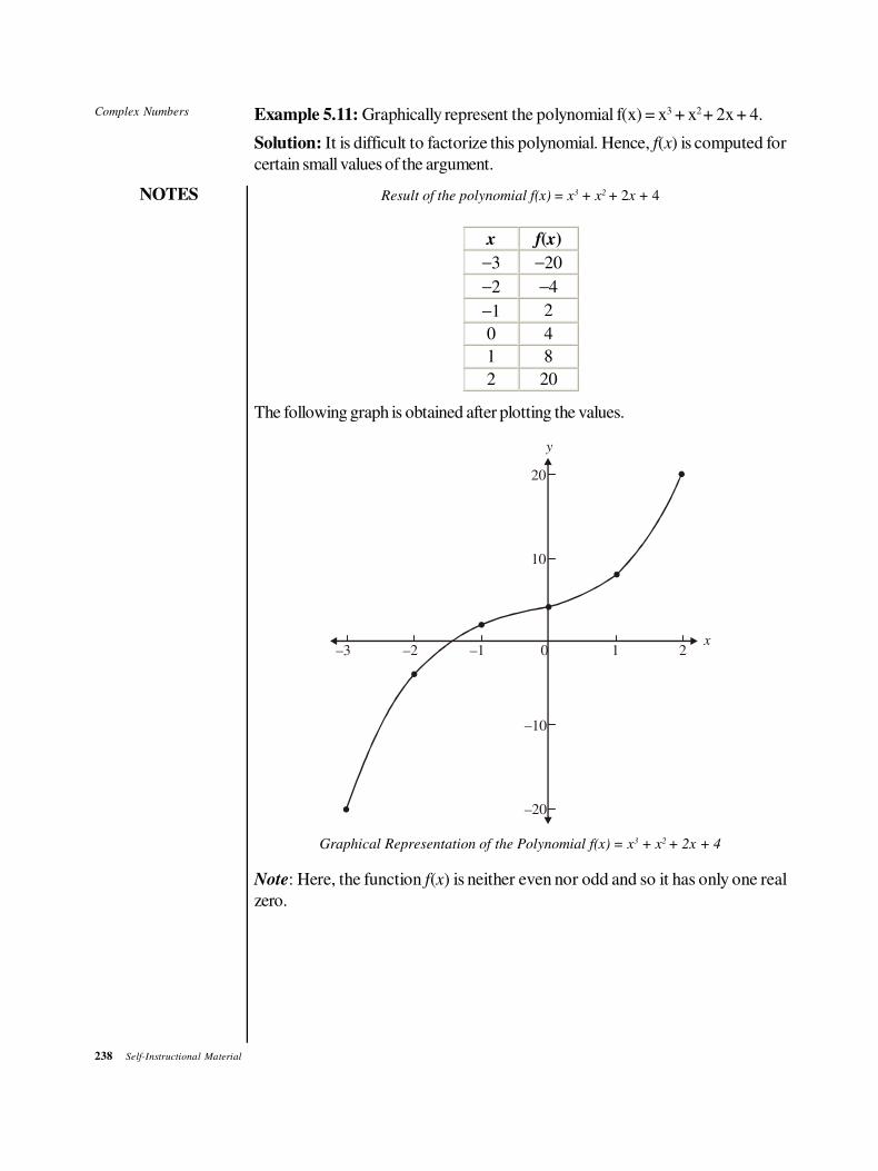
238 Self-Instructional Material
Complex Numbers
NOTES
Example 5.11: Graphically represent the polynomial f(x) = x3 + x2 + 2x + 4.
Solution: It is difficult to factorize this polynomial. Hence, f(x) is computed for
certain small values of the argument.
Result of the polynomial f(x) = x3 + x2 + 2x + 4
x f(x)
−3 −20
−2 −4
−1 2
0 4
1 8
2 20
The following graph is obtained after plotting the values.
x
y
–3 –2 –1 1 20
20
10
–10
–20
Graphical Representation of the Polynomial f(x) = x3 + x2 + 2x + 4
Note: Here, the function f(x) is neither even nor odd and so it has only one real
zero.
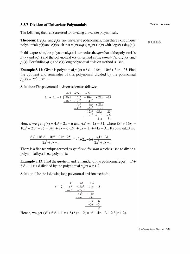
Complex Numbers
NOTES
Self-Instructional Material 239
5.3.7 Division of Univariate Polynomials
The following theorems are used for dividing univariate polynomials.
Theorem: If p1(x) and p
2(x) are univariate polynomials, then there exist unique
polynomials q(x) and r(x) such that p1(x) = q(x) p
2(x) + r(x) with deg(r) < deg(p
2).
In this expression, the polynomial q(x) is termed as the quotient of the polynomials
p1(x) and p
2(x) and the polynomial r(x) is termed as the remainder of p
1(x) and
p2(x). For finding q(x) and r(x) long polynomial division method is used.
Example 5.12: Given is polynomial p1(x) = 8x4 + 16x3 − 10x2 + 21x − 25. Find
the quotient and remainder of this polynomial divided by the polynomial
p2(x) = 2x2 + 3x − 1.
Solution: The polynomial division is done as follows:
2 + 3 – 1 8 16 – 10 + 21 –25 – – 2 + 4 4 6 21 12 +23 – 5 18 6
41 –31
x x x x x x4 3 2
8 1 – + – 4 –6 + 2
– 2 12 + –
x x x
x x x
x x x
x x
x x
x
4 3 2
3 2
3 2
2
2
4 +2 – 6 x x2
Hence, we get q(x) = 4x2 + 2x − 6 and r(x) = 41x − 31, where 8x4 + 16x3 −10x2 + 21x − 25 = (4x2 + 2x − 6)(2x2 + 3x − 1) + 41x − 31. Its equivalent is,
4 3 22
2 2
8 16 10 21 25 41 314 2 6
2 3 1 2 3 1
x x x x xx x
x x x x
+ − + − −= + − +
+ − + −
There is a fine technique termed as synthetic division which is used to divide a
polynomial by a linear polynomial.
Example 5.13: Find the quotient and remainder of the polynomial p1(x) = x3 +
6x2 + 11x + 8 divided by the polynomial p2(x) = x + 2.
Solution: Use the following long polynomial division method:
x + x x x + 2 16 + 11 8 – –2 4 +
3 + 2
x x
x x
x x
x
x
3 +11– 4 –8
3 8 – 3 –6
2
2
2
2
x x +2 +4 3
Hence, we get (x3 + 6x2 + 11x + 8) / (x + 2) = x2 + 4x + 3 + 2 / (x + 2).
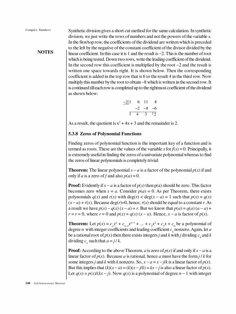
240 Self-Instructional Material
Complex Numbers
NOTES
Synthetic division gives a short cut method for the same calculation. In synthetic
division, we just write the rows of numbers and not the powers of the variable x.
In the first/top row, the coefficients of the dividend are written which is preceded
to the left by the negative of the constant coefficient of the divisor divided by the
linear coefficient. In this case it is 1 and the result is −2. This is the number of root
which is being tested. Down two rows, write the leading coefficient of the dividend.
In the second row this coefficient is multiplied by the root −2 and the result is
written one space towards right. It is shown below. Then the corresponding
coefficient is added in the top row that is 6 to the result 4 in the third row. Now
multiply this number by the root to obtain −8 which is written in the second row. It
is continued till each row is completed up to the rightmost coefficient of the dividend
as shown below:
1 6 11 82
2 8 6
|1 4 3 2
−
− − −
As a result, the quotient is x2 + 4x + 3 and the remainder is 2.
5.3.8 Zeros of Polynomial Functions
Finding zeros of polynomial function is the important key of a function and is
termed as roots. These are the values of the variable x for f(x) = 0. Principally, it
is extremely useful in finding the zeros of a univariate polynomial whereas to find
the zeros of linear polynomials is completely trivial.
Theorem: The linear polynomial x − a is a factor of the polynomial p(x) if and
only if a is a zero of f and also p(a) = 0.
Proof: Evidently if x − a is a factor of p(x) then p(a) should be zero. This factor
becomes zero when x = a. Consider p(a) = 0. As per Theorem, there exists
polynomials q(x) and r(x) with deg(r) < deg(x − a) = 1 such that p(x) = q(x)
(x − a) + r(x). Because deg(r)=0, hence, r(x) should be equal to a constant r. As
a result we have p(x) − q(x) (x − a) + r. But we know that p(a) = q(a) (a − a) +
r = r = 0, where r = 0 and p(x) = q(x) (x − a). Hence, x − a is factor of p(x).
Theorem: Let p(x) = cnxn + c
n–1xn–1 + ... + c
2x2 + c
1x + c
0 be a polynomial of
degree n with integer coefficients and leading coefficient cn nonzero. Again, let a
be a rational root of p(x) then there exists integers j and k with j dividing c0 and k
dividing cn such that a = j / k.
Proof: According to the above Theorem, a is zero of p(x) if and only if x − a is a
linear factor of p(x). Because a is rational, hence a must have the form j / k for
some integers j and k with k nonzero. So, x − a = x − j/k is a linear factor of p(x).
But this implies that (k)(x − a) = (k)(x − j/k) = kx − j is also a linear factor of p(x).
Let q(x) = p(x)/(kx − j). Now q(x) is a polynomial of degree n − 1 with integer
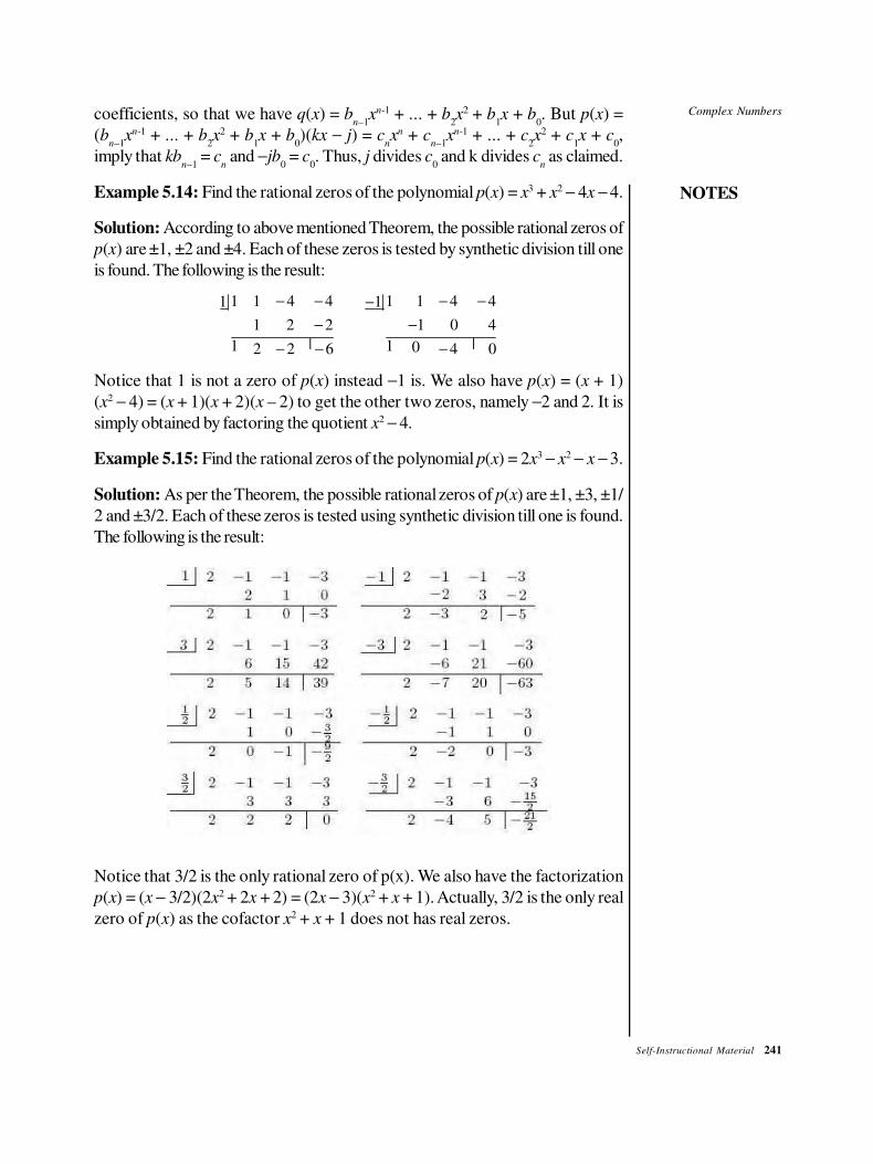
Complex Numbers
NOTES
Self-Instructional Material 241
coefficients, so that we have q(x) = bn–1
xn-1 + ... + b2x2 + b
1x + b
0. But p(x) =
(bn–1
xn-1 + ... + b2x2 + b
1x + b
0)(kx − j) = c
nxn + c
n–1xn-1 + ... + c
2x2 + c
1x + c
0,
imply that kbn–1
= cn and −jb
0 = c
0. Thus, j divides c
0 and k divides c
n as claimed.
Example 5.14: Find the rational zeros of the polynomial p(x) = x3 + x2 − 4x − 4.
Solution: According to above mentioned Theorem, the possible rational zeros of
p(x) are ±1, ±2 and ±4. Each of these zeros is tested by synthetic division till one
is found. The following is the result:
1 1 4 4 1 1 4 41 1
1 2 2 1 0 4
| |1 1 02 2 6 4 0
− − − −−
− −
− − −
Notice that 1 is not a zero of p(x) instead −1 is. We also have p(x) = (x + 1)
(x2 − 4) = (x + 1)(x + 2)(x – 2) to get the other two zeros, namely −2 and 2. It is
simply obtained by factoring the quotient x2 − 4.
Example 5.15: Find the rational zeros of the polynomial p(x) = 2x3 − x2 − x − 3.
Solution: As per the Theorem, the possible rational zeros of p(x) are ±1, ±3, ±1/
2 and ±3/2. Each of these zeros is tested using synthetic division till one is found.
The following is the result:
Notice that 3/2 is the only rational zero of p(x). We also have the factorization
p(x) = (x − 3/2)(2x2 + 2x + 2) = (2x − 3)(x2 + x + 1). Actually, 3/2 is the only real
zero of p(x) as the cofactor x2 + x + 1 does not has real zeros.
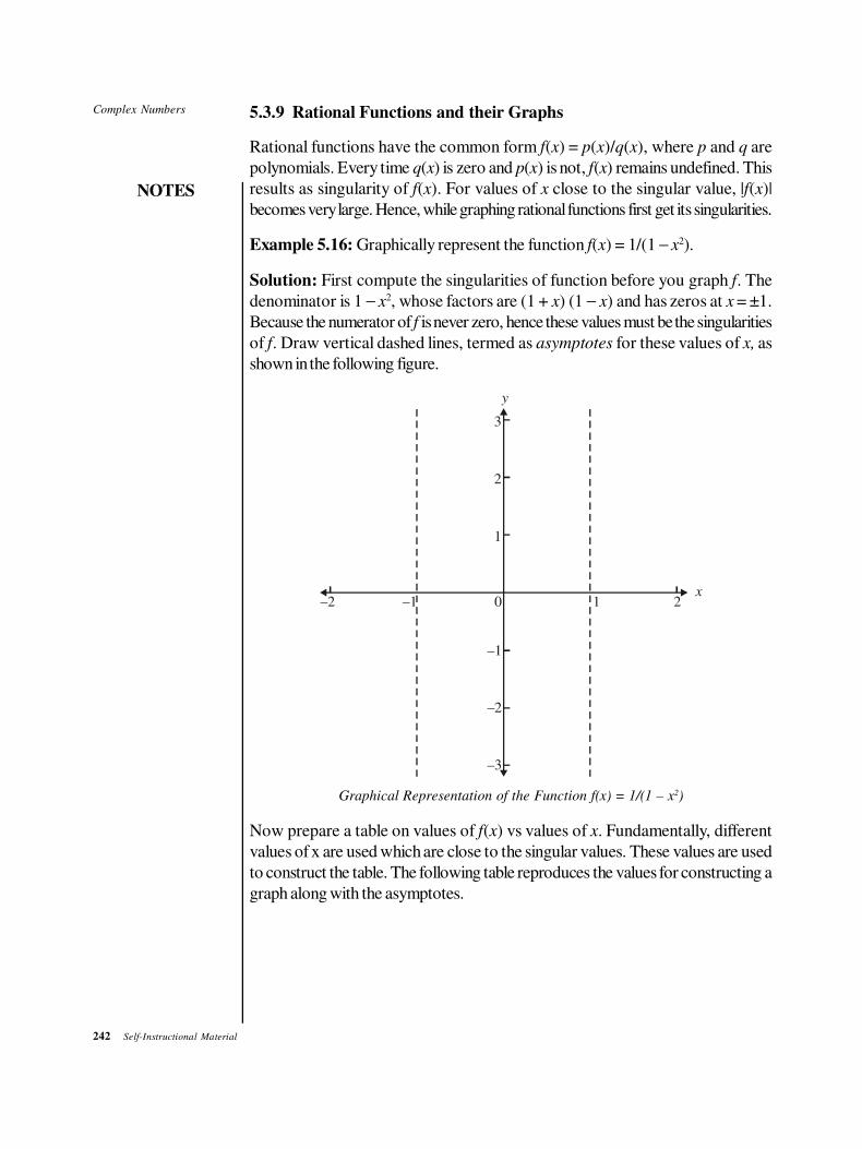
242 Self-Instructional Material
Complex Numbers
NOTES
5.3.9 Rational Functions and their Graphs
Rational functions have the common form f(x) = p(x)/q(x), where p and q are
polynomials. Every time q(x) is zero and p(x) is not, f(x) remains undefined. This
results as singularity of f(x). For values of x close to the singular value, |f(x)|
becomes very large. Hence, while graphing rational functions first get its singularities.
Example 5.16: Graphically represent the function f(x) = 1/(1 − x2).
Solution: First compute the singularities of function before you graph f. The
denominator is 1 − x2, whose factors are (1 + x) (1 − x) and has zeros at x = ±1.
Because the numerator of f is never zero, hence these values must be the singularities
of f. Draw vertical dashed lines, termed as asymptotes for these values of x, as
shown in the following figure.
–2 –1 1 20
–1
–2
–3
3
2
1
x
y
Graphical Representation of the Function f(x) = 1/(1 – x2)
Now prepare a table on values of f(x) vs values of x. Fundamentally, different
values of x are used which are close to the singular values. These values are used
to construct the table. The following table reproduces the values for constructing a
graph along with the asymptotes.
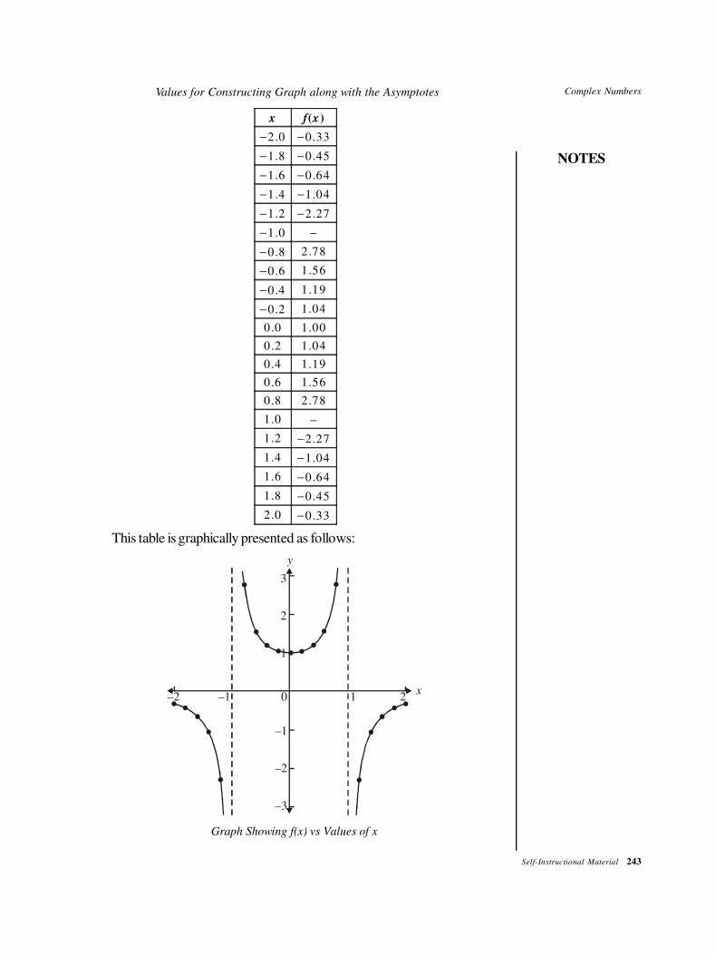
Complex Numbers
NOTES
Self-Instructional Material 243
Values for Constructing Graph along with the Asymptotes
x f(x)
−2.0 −0.33
−1.8 −0.45
−1.6 −0.64
−1.4 −1.04
−1.2 −2.27
−1.0 −
−0.8 2.78
−0.6 1.56
−0.4 1.19
−0.2 1.04
0.0 1.00
0.2 1.04
0.4 1.19
0.6 1.56
0.8 2.78
1.0 −
1.2 −2.27
1.4 −1.04
1.6 −0.64
1.8 −0.45
2.0 −0.33
This table is graphically presented as follows:
x
y
–2 –1 0 1 2
3
2
1
–1
–2
–3
Graph Showing f(x) vs Values of x
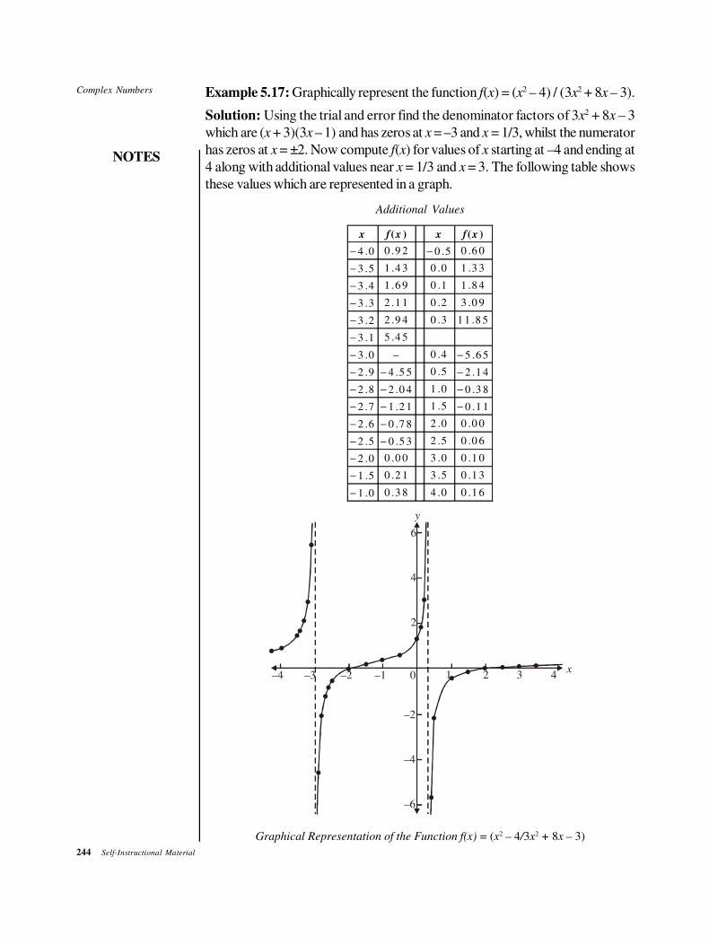
244 Self-Instructional Material
Complex Numbers
NOTES
Example 5.17: Graphically represent the function f(x) = (x2 – 4) / (3x2 + 8x – 3).
Solution: Using the trial and error find the denominator factors of 3x2 + 8x – 3
which are (x + 3)(3x – 1) and has zeros at x = –3 and x = 1/3, whilst the numerator
has zeros at x = ±2. Now compute f(x) for values of x starting at –4 and ending at
4 along with additional values near x = 1/3 and x = 3. The following table shows
these values which are represented in a graph.
Additional Values
x f(x ) x f(x )
− 4 .0 0 .9 2 − 0 .5 0 .6 0
− 3 .5 1 .4 3 0 .0 1 .3 3
− 3 .4 1 .6 9 0 .1 1 .8 4
− 3 .3 2 .1 1 0 .2 3 .0 9
− 3 .2 2 .9 4 0 .3 1 1 .8 5
− 3 .1 5 .4 5
− 3 .0 − 0 .4 − 5 .6 5
− 2 .9 − 4 .5 5 0 .5 − 2 .1 4
− 2 .8 − 2 .0 4 1 .0 − 0 .3 8
− 2 .7 − 1 .2 1 1 .5 − 0 .1 1
− 2 .6 − 0 .7 8 2 .0 0 .0 0
− 2 .5 − 0 .5 3 2 .5 0 .0 6
− 2 .0 0 .0 0 3 .0 0 .1 0
− 1 .5 0 .2 1 3 .5 0 .1 3
− 1 .0 0 .3 8 4 .0 0 .1 6
–4 –3 –2 –1 0 1 2 3 4x
–2
–4
–6
6
4
2
y
Graphical Representation of the Function f(x) = (x2 – 4/3x2 + 8x – 3)
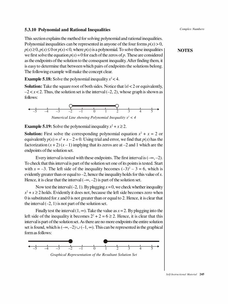
Complex Numbers
NOTES
Self-Instructional Material 245
5.3.10 Polynomial and Rational Inequalities
This section explains the method for solving polynomial and rational inequalities.
Polynomial inequalities can be represented in anyone of the four forms p(x) > 0,
p(x) ≥ 0, p(x) ≤ 0 or p(x) < 0, where p(x) is a polynomial. To solve these inequalities
we first solve the equation p(x) = 0 for each of the zeros of p. These are considered
as the endpoints of the solution to the consequent inequality. After finding them, it
is easy to determine that between which pairs of endpoints the solutions belong.
The following example will make the concept clear.
Example 5.18: Solve the polynomial inequality x2 < 4.
Solution: Take the square root of both sides. Notice that |x| < 2 or equivalently,
–2 < x < 2. Thus, the solution set is the interval (–2, 2), whose graph is shown as
follows:
–5 –4 –3 –2 –1 0 1 2 3 4 5
Numerical Line showing Polynomial Inequality x2 < 4
Example 5.19: Solve the polynomial inequality x2 + x ≥ 2.
Solution: First solve the corresponding polynomial equation x2 + x = 2 or
equivalently p(x) = x2 + x – 2 = 0. Using trial and error, we find that p(x) has the
factorization (x + 2) (x – 1) implying that its zeros are at –2 and 1 which are the
endpoints of the solution set.
Every interval is tested with these endpoints. The first interval is (–∞, –2).
To check that this interval is part of the solution set one of its points is tested. Start
with x = –3. The left side of the inequality becomes (–3)2 – 3 = 6, which is
evidently greater than or equal to –2, hence the inequality holds for this value of x.
Hence, it is clear that the interval (–∞, –2) is part of the solution set.
Now test the interval (–2, 1). By plugging x = 0, we check whether inequality
x2 + x ≥ 2 holds. Evidently it does not, because the left side becomes zero when
0 is substituted for x and 0 is not greater than or equal to 2. Hence, it is clear that
the interval (–2, 1) is not part of the solution set.
Finally test the interval (1, ∞). Take the value as x = 2. By plugging into the
left side of the inequality it becomes 22 + 2 = 6 ≥ 2. Hence, it is clear that this
interval is part of the solution set. As there are no more endpoints the entire solution
set is found, which is (–∞, –2) ∪ (–1, ∞). This can be represented in the graphical
form as follows:
–5 –4 –3 –2 –1 0 1 2 3 4 5
Graphical Representation of the Resultant Solution Set
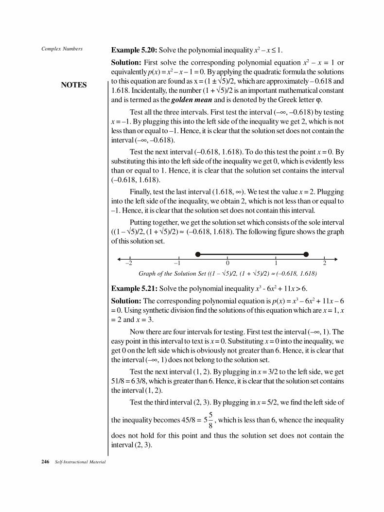
246 Self-Instructional Material
Complex Numbers
NOTES
Example 5.20: Solve the polynomial inequality x2 – x ≤ 1.
Solution: First solve the corresponding polynomial equation x2 – x = 1 or
equivalently p(x) = x2 – x – 1 = 0. By applying the quadratic formula the solutions
to this equation are found as x = (1 ± √5)/2, which are approximately – 0.618 and
1.618. Incidentally, the number (1 + √5)/2 is an important mathematical constant
and is termed as the golden mean and is denoted by the Greek letter ϕ.
Test all the three intervals. First test the interval (–∞, –0.618) by testing
x = –1. By plugging this into the left side of the inequality we get 2, which is not
less than or equal to –1. Hence, it is clear that the solution set does not contain the
interval (–∞, –0.618).
Test the next interval (–0.618, 1.618). To do this test the point x = 0. By
substituting this into the left side of the inequality we get 0, which is evidently less
than or equal to 1. Hence, it is clear that the solution set contains the interval
(–0.618, 1.618).
Finally, test the last interval (1.618, ∞). We test the value x = 2. Plugging
into the left side of the inequality, we obtain 2, which is not less than or equal to
–1. Hence, it is clear that the solution set does not contain this interval.
Putting together, we get the solution set which consists of the sole interval
((1 – √5)/2, (1 + √5)/2) ≈ (–0.618, 1.618). The following figure shows the graph
of this solution set.
–2 –1 0 1 2
Graph of the Solution Set ((1 – √5)/2, (1 + √5)/2) ≈ (–0.618, 1.618)
Example 5.21: Solve the polynomial inequality x3 - 6x2 + 11x > 6.
Solution: The corresponding polynomial equation is p(x) = x3 – 6x2 + 11x – 6
= 0. Using synthetic division find the solutions of this equation which are x = 1, x
= 2 and x = 3.
Now there are four intervals for testing. First test the interval (–∞, 1). The
easy point in this interval to text is x = 0. Substituting x = 0 into the inequality, we
get 0 on the left side which is obviously not greater than 6. Hence, it is clear that
the interval (–∞, 1) does not belong to the solution set.
Test the next interval (1, 2). By plugging in x = 3/2 to the left side, we get
51/8 = 6 3/8, which is greater than 6. Hence, it is clear that the solution set contains
the interval (1, 2).
Test the third interval (2, 3). By plugging in x = 5/2, we find the left side of
the inequality becomes 45/8 = 5
58
, which is less than 6, whence the inequality
does not hold for this point and thus the solution set does not contain the
interval (2, 3).
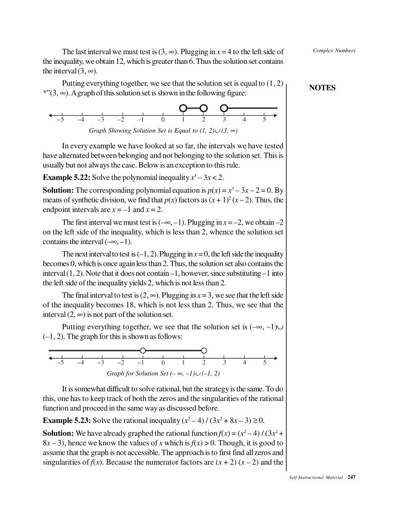
Complex Numbers
NOTES
Self-Instructional Material 247
The last interval we must test is (3, ∞). Plugging in x = 4 to the left side of
the inequality, we obtain 12, which is greater than 6. Thus the solution set contains
the interval (3, ∞).
Putting everything together, we see that the solution set is equal to (1, 2)
*”(3, ∞). A graph of this solution set is shown in the following figure:
–5 –4 –3 –2 –1 0 1 2 3 4 5
Graph Showing Solution Set is Equal to (1, 2)∪ (3, ∞)
In every example we have looked at so far, the intervals we have tested
have alternated between belonging and not belonging to the solution set. This is
usually but not always the case. Below is an exception to this rule.
Example 5.22: Solve the polynomial inequality x3 – 3x < 2.
Solution: The corresponding polynomial equation is p(x) = x3 – 3x – 2 = 0. By
means of synthetic division, we find that p(x) factors as (x + 1)2 (x – 2). Thus, the
endpoint intervals are x = –1 and x = 2.
The first interval we must test is (–∞, –1). Plugging in x = –2, we obtain –2
on the left side of the inequality, which is less than 2, whence the solution set
contains the interval (–∞, –1).
The next interval to test is (–1, 2). Plugging in x = 0, the left side the inequality
becomes 0, which is once again less than 2. Thus, the solution set also contains the
interval (1, 2). Note that it does not contain –1, however, since substituting –1 into
the left side of the inequality yields 2, which is not less than 2.
The final interval to test is (2, ∞). Plugging in x = 3, we see that the left side
of the inequality becomes 18, which is not less than 2. Thus, we see that the
interval (2, ∞) is not part of the solution set.
Putting everything together, we see that the solution set is (–∞, –1)∪(–1, 2). The graph for this is shown as follows:
–5 –4 –3 –2 –1 0 1 2 3 4 5
Graph for Solution Set (– ∞, –1)∪ (–1, 2)
It is somewhat difficult to solve rational, but the strategy is the same. To do
this, one has to keep track of both the zeros and the singularities of the rational
function and proceed in the same way as discussed before.
Example 5.23: Solve the rational inequality (x2 – 4) / (3x2 + 8x – 3) ≥ 0.
Solution: We have already graphed the rational function f(x) = (x2 – 4) / (3x2 +
8x – 3), hence we know the values of x which is f(x) > 0. Though, it is good to
assume that the graph is not accessible. The approach is to first find all zeros and
singularities of f(x). Because the numerator factors are (x + 2) (x – 2) and the
248 Self-Instructional Material
Complex Numbers
NOTES
denominator factors are (x + 3) (3x – 1), we observe that the zeros of f are at
–2 and 2 and the singularities are –3 and 1/3. These are the endpoints of the
intervals.
Test the first interval (–∞, –3). Because f(–10) = 96 / 217 > 0, hence, it is
clear that this interval belongs to the solution set.
Test the second interval (–3, –2). We have f(–5/2) = –17/4 < 0, hence, it is
clear that this interval does not belong to the solution set.
Test the third interval (–2, 1/3). Since f(0) = 4/3 > 0, hence it is clear that
this interval belongs to the solution set.
Now test the fourth interval (1/3, 2). We have f(1) = –3/8 < 0, hence it is
clear that this interval does not belong to the solution set.
Finally test the last interval (2, ∞). We have f(10) = 96 / 377 > 0, hence it
is clear that this interval belongs to the solution set.
Putting the findings together, we find the solution set (–∞, –3] ∪ [–2, 1/3]
∪ [2, ∞). The graph for the obtained solution set is shown as follows:
–5 –4 –3 –2 –1 0 1 2 3 4 5
Graph for the Obtained Solution Set (– ∞, – 3] ∪ [–2, 1/3] ∪ [2, ∞)
CHECK YOUR PROGRESS
5. Can two parts of a complex number be represented graphically?
6. Which is the important key of a function?
7. What do you understand by the singularity of f(x)?
8. How can polynomial inequalities be represented?
5.4 USES OF COMPLEX NUMBERS
Complex number finds use in a number of scientific and engineering calculations.
While solving an equation, if the solution yields square root of a negative number,
there it indicates presence of a complex number. In the field of electrical engineering
and telecommunication complex numbers come. Although a complex number
involves imaginary number it has correspondence to the real word situation. As
you have seen, a complex number can be given a graphical addition in place of
direct arithmetic addition.
5.4.1 History of Complex Numbers
Reference for square roots negative real numbers was found in the work of Heron
of Alexandria, the Greek during 1st century AD. He felt it by considering volume
of the frustum of a pyramid that was considered impossible. These problems of
square root of negative number became very prominent by work of Italian
Complex Numbers
NOTES
Self-Instructional Material 249
mathematicians in finding third and fourth roots of polynomials. Although main
interest was in finding the real solution but, they were also interested in manipulating
square roots of negative numbers. The term ‘imaginary’ for such quantities was
first coined by Rene Descartes during the period of 17th century. This term was
used to mean derogatory. In the period of 18th century, work of Leonhard Euler
and Abraham De Moivre established many concepts related to complex numbers.
Famous formulae, known as De Moivre’s theorem was given on his name.
According to De Moivre’s theorem:
(cosθ + isinθ)n = cosnθ + isinnθ
Where θ is any complex number or real number and n is an integer.
This formula is considered very important as it connects a complex numbers
to trigonometry. The expression ‘cos θ + i sin θ’ is also known as ‘cis θ’ in short.
We may expand LHS of the De Moivre’s formula and after comparing both
the parts (assuming that θ is a real number), expressions can be derived for cos(nθ)
and sin(nθ) involving terms of cos(θ) and sin(θ). Also, this formula can be used for
finding nth roots of unity. We can find a complex number z such that zn = 1.
Existence of complex numbers was accepted only after its geometrical
interpretation was given by Caspar Wessel in the year 1799. Same thing was
discovered later after several years. This was popularized by Gauss (Carl Friedrich
Gauss) and due to his efforts complex numbers theory got further expansion.
Wessel’s memoir was given in Proceedings of the Copenhagen Academy in
1799. This work is complete and very clear in content that can be compared to
any modern work. He considered sphere, and provided a quaternion theory that
can develop spherical trigonometry. In the year 1806 Argand got the same idea
that was suggested by Wallis and also issued a paper on this subject. Argand’s
essay provided a base on which present day graphic presentation of complex
numbers works. In 1832 Gauss published his work on it and brought it in
mathematical world, giving it a prominence. Mention should also be made of the
excellent small treatise presented by Mourey in the year 1828. In this period
foundations were laid scientifically for the theory of directional numbers.
Different terms were used by different mathematician in relation to complex
number. Argand called cosθ + isinθ the direction factor, and the modulus. Cauchy,
in the year 1828 called the same as the reduced form and Gauss used i for square
root of –1 and (imaginary number) and used the term complex number for a
binomial term a + bi, and named a2 + b2 as the norm. Hankel, in the year 1867,
used direction coefficient, for expression ‘cosθ+isinθ’. The term absolute value,
for modulus, was used by Weierstrass.
After Cauchy and Gauss, many names came as high ranking contributors.
Of these, following names are worth mention:
Contribution was made in 1844 by Kummer, in 1845 by Kronecker,
Leopold and Peacock and Scheffler in 1845, 1851 and 1880 and Bellavitis in
1835 and 1852.
250 Self-Instructional Material
Complex Numbers
NOTES
Also, Scheffler (1845, 1851, 1880), Bellavitis (1835, 1852), Peacock
(1845), and De Morgan (1849) were great contributors. Name of Möbius is also
worth mention for his numerous works on geometric applications of complex
numbers. The work of Dirichlet helped expansion of this theory that included
complex numbers for primes, congruences, reciprocity, and like that as was for
real numbers.
A set of complex number, closed under addition, subtraction and
multiplication, is known as complex ring or field. Study was made for complex
numbers having form a + bi. [a and b being integral, or rational and i is here either
of the two roots of x2 + 1 = 0]. Ferdinand Eisenstein who was his student, carried
study of the type a + bω, where ω is the complex cubic root (complex root of
x3 – 1 = 0). There were other classes too for such cases and these are known as
cyclotomic fields for complex numbers. These have been derived from equation
xk – 1 = 0, by finding roots of unity in case of higher values of k. Such generalization
was mainly due to the work Kummer, who invented ideal numbers, expressed as
geometrical entities by Felix Klein in 1893. General theory for fields had been
created by Évariste Galois. He carried out study on fields that was generated by
roots of a polynomial equation in one variable.
Complex numbers, thus have a field, known as complex number field and is
denoted by C. A complex number x + iy, is denoted as an ordered pair of (x, y).
A number whose imaginary part is zero is a real number. A number, whose real
part is zero, is a purely imaginary number and a number whose neither part is zero
is a complex number. Viewing this way every real number is a subset of complex
number. Or stated in terms of field one may say that R, the field of real numbers is
a subfield of C. Thus, we identify a real number x as complex number (x, 0) and
an imaginary number may be denoted as complex number (0, y).
In the field of complex number C, we have:
Additive identity as (0,0), multiplicative identity as (1,0), additive inverse of
(x, y) as (– x, – y)
Thus, complex field C can also be defined as the topological closure of
algebraic numbers and the algebraic closure of R.
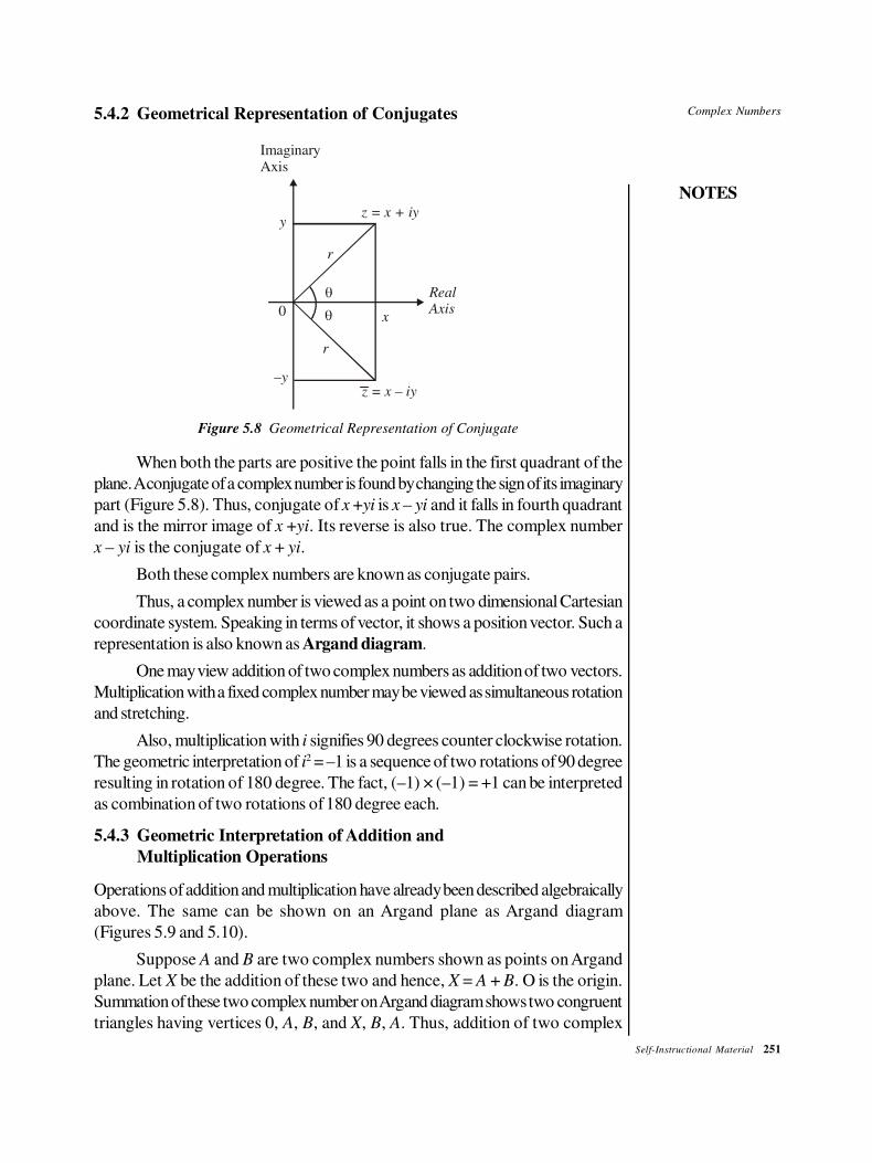
Complex Numbers
NOTES
Self-Instructional Material 251
5.4.2 Geometrical Representation of Conjugates
ImaginaryAxis
yz = x + iy
r
Real
Axisx
–y
0
r
z = x – iy
Figure 5.8 Geometrical Representation of Conjugate
When both the parts are positive the point falls in the first quadrant of the
plane. A conjugate of a complex number is found by changing the sign of its imaginary
part (Figure 5.8). Thus, conjugate of x +yi is x – yi and it falls in fourth quadrant
and is the mirror image of x +yi. Its reverse is also true. The complex number
x – yi is the conjugate of x + yi.
Both these complex numbers are known as conjugate pairs.
Thus, a complex number is viewed as a point on two dimensional Cartesian
coordinate system. Speaking in terms of vector, it shows a position vector. Such a
representation is also known as Argand diagram.
One may view addition of two complex numbers as addition of two vectors.
Multiplication with a fixed complex number may be viewed as simultaneous rotation
and stretching.
Also, multiplication with i signifies 90 degrees counter clockwise rotation.
The geometric interpretation of i2 = –1 is a sequence of two rotations of 90 degree
resulting in rotation of 180 degree. The fact, (–1) × (–1) = +1 can be interpreted
as combination of two rotations of 180 degree each.
5.4.3 Geometric Interpretation of Addition and
Multiplication Operations
Operations of addition and multiplication have already been described algebraically
above. The same can be shown on an Argand plane as Argand diagram
(Figures 5.9 and 5.10).
Suppose A and B are two complex numbers shown as points on Argand
plane. Let X be the addition of these two and hence, X = A + B. O is the origin.
Summation of these two complex number on Argand diagram shows two congruent
triangles having vertices 0, A, B, and X, B, A. Thus, addition of two complex
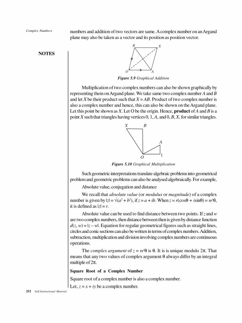
252 Self-Instructional Material
Complex Numbers
NOTES
numbers and addition of two vectors are same. A complex number on an Argand
plane may also be taken as a vector and its position as position vector.
B X
O A
Figure 5.9 Graphical Addition
Multiplication of two complex numbers can also be shown graphically by
representing them on Argand plane. We take same two complex number A and B
and let X be their product such that X = AB. Product of two complex number is
also a complex number and hence, this can also be shown on the Argand plane.
Let this point be shown as X. Let O be the origin. Hence, product of A and B is a
point X such that triangles having vertices 0, 1, A, and 0, B, X, for similar triangles.
X B
A
O1
Figure 5.10 Graphical Multiplication
Such geometric interpretations translate algebraic problems into geometrical
problem and geometric problems can also be analysed algebraically. For example,
Absolute value, conjugation and distance
We recall that absolute value (or modulus or magnitude) of a complex
number is given by |z| = √(a2 + b2), if z = a + ib. When z = r(cosθ + isinθ) = reiθ,
it is defined as |z| = r.
Absolute value can be used to find distance between two points. If z and w
are two complex numbers, then distance between then is given by distance function
d(z, w) = |z – w|. Equation for regular geometrical figures such as straight lines,
circles and conic sections can also be written in terms of complex numbers. Addition,
subtraction, multiplication and division involving complex numbers are continuous
operations.
The complex argument of z = reiθ is θ. It is is unique modulo 2π. That
means that any two values of complex argument θ always differ by an integral
multiple of 2π.
Square Root of a Complex Number
Square root of a complex number is also a complex number.
Let, z = x + iy be a complex number.
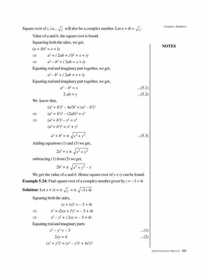
Complex Numbers
NOTES
Self-Instructional Material 253
Square root of z, i.e., z will also be a complex number. Let a + ib = z .
Value of a and b, the square root is found.
Squarring both the sides, we get,
(a + ib)2 = x + iy
⇒ a2 + i 2ab + z2b2 = x + iy
⇒ a2 – b2 + i 2ab = x + iy
Equating real and imaginary part together, we get,
a2
– b2 + i 2ab = x + iy
Equating real and imaginary part together, we get,
a2 – b2 = x ...(5.1)
2 ab = y ...(5.2)
We know that,
(a2 + b2)2 – 4a2b2 = (a2 – b2)2
⇒ (a2 + b2)2 – (2ab)2 = x2
⇒ (a2 + b2)2 – y2 = x2
(a2 + b2)2 = x2 + y2
a2 + b2 = ± 2 2x y+ ...(5.3)
Adding equations (1) and (3) we get,
2a2 = x ± 2 2x y+
subtracting (1) from (3) we get,
2b2 = ± 2 2x y+ – x
We get the value of a and b. Hence square root of x + iy can be found.
Example 5.24: Find square root of a complex number given by z = – 3 + 4i
Solution: Let x + iy = ± z = ± 3 4i− +
Squaring both the sides,
(x + iy)2 = – 3 + 4i
⇒ x2 + i2xy + i2y2 = – 3 + 4i
⇒ x2 – y2 + i 2xy = – 3 + 4i
Equating real and imaginary parts
x2 – y2 = – 3 ...(1)
2xy = 4 ...(2)
(x2 + y2)2 = (x2 – y2)2 + 4x2y2
254 Self-Instructional Material
Complex Numbers
NOTES
= (–3)2 + (4)2 = 9 + 16 = 25
⇒ (x2 + y2)2 = 25
x2 + y2 = ± 5 ...(3)
Adding equations (1) and (3), we get
2x2 = – 3 ± 5 = 2 or – 8
⇒ x = ± 1 or ± 2i
Since x is a real number, we take x = ± 1, and discard imaginary value.
2xy = 4 given
y = 4
2x =
4
2 ( 1)× ± = ± 2.
When x = 1, y = 2,
x = –1, y = –2
We get square root of –3 + 4i
as
(1) 1 + 2i,
(2) – 1 – 2i,
Hence, square root of – 3 + 4i
is ± (1 + 2i).
Example 5.25: Find square root of a complex number given as:
z = 7 + 24i
Solution: Let
x + iy = ± 7 24i+
Squarring both the sides,
x2 + i2xy + i2y2 = 7 24i+
⇒ x2 – y2 + i 2xy = 7 + 24i
x2 – y2 = 7 ...(1)
2xy = 24 ...(2)
(x2 + y2)2 = (x2 – y2)2 + 4x2y2
= (x2 – y2)2 + (2xy)2
= (7)2 + (24)
= 49 + 576
= 625
x2 + y2 = ± 25 ...(3)
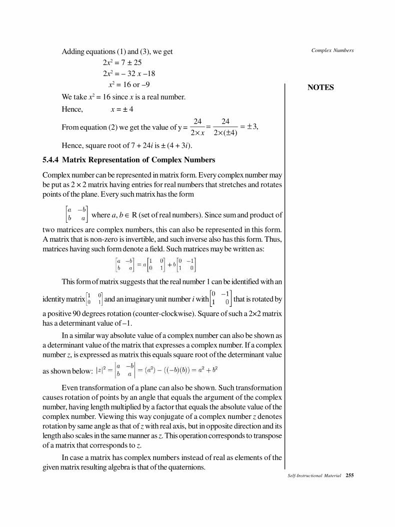
Complex Numbers
NOTES
Self-Instructional Material 255
Adding equations (1) and (3), we get
2x2 = 7 ± 25
2x2 = – 32 x –18
x2 = 16 or –9
We take x2 = 16 since x is a real number.
Hence, x = ± 4
From equation (2) we get the value of y = 24 24
3,2 2 ( 4)x
= = ±× × ±
Hence, square root of 7 + 24i is ± (4 + 3i).
5.4.4 Matrix Representation of Complex Numbers
Complex number can be represented in matrix form. Every complex number may
be put as 2 × 2 matrix having entries for real numbers that stretches and rotates
points of the plane. Every such matrix has the form
where a, b ∈ R (set of real numbers). Since sum and product of
two matrices are complex numbers, this can also be represented in this form.
A matrix that is non-zero is invertible, and such inverse also has this form. Thus,
matrices having such form denote a field. Such matrices may be written as:
This form of matrix suggests that the real number 1 can be identified with an
identity matrix and an imaginary unit number i with that is rotated by
a positive 90 degrees rotation (counter-clockwise). Square of such a 2×2 matrix
has a determinant value of –1.
In a similar way absolute value of a complex number can also be shown as
a determinant value of the matrix that expresses a complex number. If a complex
number z, is expressed as matrix this equals square root of the determinant value
as shown below:
Even transformation of a plane can also be shown. Such transformation
causes rotation of points by an angle that equals the argument of the complex
number, having length multiplied by a factor that equals the absolute value of the
complex number. Viewing this way conjugate of a complex number z denotes
rotation by same angle as that of z with real axis, but in opposite direction and its
length also scales in the same manner as z. This operation corresponds to transpose
of a matrix that corresponds to z.
In case a matrix has complex numbers instead of real as elements of the
given matrix resulting algebra is that of the quaternions.
256 Self-Instructional Material
Complex Numbers
NOTES
5.5 PROPERTIES OF COMPLEX NUMBERS
Real Vector Space
As you have seen, a complex number also represents a vector and a set of all such
complex number, denoted by C, is a real vector space in two dimensions. Ordering
as found with real numbers does not apply to complex numbers in case of arithmetic
addition and hence C cannot have an ordered field. As a generalized statement, a
field having imaginary number cannot be ordered.
Mapping of R-linear function C → C assumes the general form as given
below:
Here, a and b are complex coefficients and can be written symbolically as
a, b ∈ C.
Here, function given as: denotes rotations that is also combined
with scaling, But the function denotes reflections that are combined
with scaling.
Solutions of Polynomial Equations
A root of a polynomial p is a complex number z satisfying the equation p(z) = 0.
An n-degree polynomials having coefficients real or complex, has exactly n complex
roots. This is the Fundamental Theorem of Algebra, and this also tells that complex
numbers are defined for an algebraically closed field.
Complex Analysis
The study of functions of a complex variable is known as complex analysis and
has enormous practical use in applied mathematics as well as in other branches of
mathematics. Often, the most natural proofs for statements in real analysis or even
number theory employ techniques from complex analysis (see prime number theorem
for an example). Unlike real functions which are commonly represented as two
dimensional graphs, complex functions have four dimensional graphs and may
usefully be illustrated by color coding a three dimensional graph to suggest four
dimensions, or by animating the complex function’s dynamic transformation of the
complex plane.
5.5.1 Applications of Complex Numbers
Complex number finds various applications in many fields of science and
engineering. It is widely used in the field of control theory in electrical engineering
and telecommunication .
Control Theory
In most of the control theory in the field of telecommunication, transformation is
done from the domain of time to that of frequency. Laplace transform is used in the
field of electrical engineering for such transformations. Poles and zeros of the
Complex Numbers
NOTES
Self-Instructional Material 257
system are analyzed in complex plane. Complex plain is used in analysis of the
Nyquist plot, root locus and Nichols plot techniques.
Position of poles and holes are of special importance in the root locus method.
Situations, such as position of poles and holes with respect of quadrants is especially
important. These may lie in the left and right half planes. This is same as knowing
whether real part is greater than or less than zero. If a system has poles:
In right half of the plane - it is unstable,
All in left half of the plane - it is stable,
Falling on imaginary axis – it is marginally stable.
Also, if a system contains zeros in right half of plane, it is called non minimum
phase system.
5.5.2 Signal Analysis
In the filed of electrical engineering and telecommunication, signal analysis is done
using complex numbers to describe signals that vary periodically. Absolute value
or modulus of |z| corresponds to the amplitude and argument arg(z) as phase of a
sine wave having some given frequency.
Fourier transform and Fourier analysis is done for writing a given signal
having real value as a sum of many periodic functions, often written as the part
having real of complex functions of the form f(ε) = zeiwt. Here, ω denotes angular
frequency that is equal to 2πf, where f denotes frequency. Complex number z
does encoding of phase and amplitude.
In the fields of electrical engineering, such technique is utilized by varying
currents and voltages. In electrical systems, resistances offered by resistors are
taken as real valued and those offered by capacitors and inductors are taken as
imaginary. These three that offer combined resistance as known by another name,
impedance. Resistances offered by inductors and capacitors are known by another
name reactance.
If impedance is denoted by Z as combination of resistance R, and combined
reactance of inductor and capacitor X, then Z is denoted as a complex number as:
Z = R + i X.
Electrical engineering texts use j in place of i for showing imaginary quantity.
Improper Integrals
Complex number is used in the field of applied sciences for finding improper
integrals that are real-valued, and complex-valued functions are used for this.
There are several methods to do the same.
Quantum Mechanics
In the field of quantum mechanics also complex numbers are of importance. The
underlying theory has been built on Hilbert spaces (a space having infinite
dimensions) over C.
258 Self-Instructional Material
Complex Numbers
NOTES
Relativity
Taking time variable as imaginary use of formulas for finding metric on space time
becomes simpler.
Applied Mathematics
In solution of differential equations all complex roots r of characteristic equation is
found first for a linear differential equation. Attempts to solve for the base function
is made after this using base functions on the form f(t) = ert.
Fluid Dynamics
Complex functions, in fluid dynamics are used for describing potential flow in two
dimensions.
Fractals
Some fractals known as Julia set and Mandelbrot set are plotted in the complex
plane.
CHECK YOUR PROGRESS
9. What is a complex ring or field?
10. What is complex analysis?
5.6 SUMMARY
In this unit, you have learned that:
• Girolamo Cardano was an Italian mathematician who first realized the need
of finding complex numbers. While solving cubic equations, he came across
expressions that contained square root of a negative number. Thus, the
concept of an imaginary number took birth. However, this was accepted as
a part of mathematical concept by the work of Abraham De Moivre,
Bernoullis and Leonhard Euler, who carried out studies on this topic in
detail. De Moivre was a French-English mathematician, Bernoullis were
mathematicians in a Swiss family and Euler was also a Swiss mathematician.
This term ‘imaginary’ was used by Rene Descartes in 17th century.
• If we define that the square of imaginary number i is –1, then it is possible to
find solution of x2 + 1 = 0. In mathematics, one can describe the notions if
they satisfy a specific set of logically constant axioms. For example, the
defined number i can also be written as √–1, where the real numbers can
be included to extend it along with imaginary numbers. The simple method
to perform is to describe the set of complex numbers as the set of all numbers
of form z = x + yi, where x and y are arbitrary real numbers. Here, number
x is termed as the real part and y as the imaginary part of the complex
number z.
Complex Numbers
NOTES
Self-Instructional Material 259
• Basically, there are two functional operations on complex numbers. First is
termed as complex conjugation and the second is the modulus, also famous
as the complex norm or absolute value. For a given complex number z =
x + yi, one can describe the complex conjugate of z (written as z) as the
complex number z = x – yi such that in the complex plane, the point
corresponding to z is (x, –y).
• In a complex number, when the real part and its imaginary part are equal to
zero, then only the complex number is equal to zero. For example, a + bi
= 0 if and only if a = 0 and b = 0. Similarly, the complex numbers are equal
if their real and imaginary parts are equal.
• A complex number has two parts, real and imaginary. A number is imaginary
when it is the square root of a negative real number. For example, if x2 = 1,
then x = ± √1 = ± 1. Such a square root has both real values. But if there is
an equation x2 + 1 = 0 → x2 = – 1 and hence, x = √–1 and this number is
imaginary since there is no real number that satisfies this condition, then this
number, given by √–1, is an imaginary number and it is designated by using
letter i.
• Modulus of a complex number is a length of vector OP which represents
the complex number in a coordinate complex plane.
• Two parts of a complex number can be represented graphically by
representing one along the real axis (shown horizontally) and the other along
imaginary axis, at positive right angle to it. This is like presenting a point on
a Cartesian plane by an ordered pair (x, y).
• An Argand plane is a way to represent a complex number as points on
rectangular coordinate plane. This also known as complex plane in which
x-axis is used for real axis and y as imaginary axis. Argand plane is so
named as an amateur mathematician named Jean Robert Argand described
the plane in his paper in the year 1806.
• On an Argand plane, the position of a point can be shown both in rectangular
coordinate system as well as polar coordinate system. A complex number z
has been shown as an ordered pair (x, y) on a Cartesian plane and as (r, iθ)
in polar coordinates.
• The quadratic equations are of the form ax2 + bx + c = 0, where a, b and
c are considered as real-valued constants along with a non-zero. The left
part of this equation is a quadratic function of the form f(x) = ax2 + bx + c
and the graph of this quadratic function is termed as parabola, which is a
special type of curve. The simple parabola is specified by the function
f(x) = x2.
• The complexity of the graph depends on the degrees of polynomials growth.
A polynomial of degree n will have up to n real zeros so that its graph
crosses the x-axis n times. However, one can easily find the zeros of some
polynomials by simply plotting sufficient points. Reasonably exact graphs
can be made of general polynomials.
260 Self-Instructional Material
Complex Numbers
NOTES
• In synthetic division, we just write the rows of numbers and not the powers
of the variable x. In the first/top row, the coefficients of the dividend are
written which is preceded to the left by the negative of the constant coefficient
of the divisor divided by the linear coefficient.
• Finding zeros of polynomial function is the important key of a function,
termed as roots. These are the values of the variable x for f(x) = 0. Principally,
it is extremely useful in finding the zeros of a univariate polynomial, whereas
to find the zeros of linear polynomials is completely trivial.
• Rational functions have the common form f(x) = p(x)/q(x), where p and q
are polynomials. When q(x) is zero and p(x) is not, f(x) remains undefined.
This results as singularity of f(x). For values of x close to the singular value,
|f(x)| becomes very large. Hence, while graphing rational functions first check
its singularities.
• Polynomial inequalities can be represented in any one of the four forms,
p(x) > 0, p(x) ≥ 0, p(x) ≤ 0 or p(x) < 0, where p(x) is a polynomial. To
solve these inequalities, we first solve the equation p(x) = 0 for each of the
zeros of p. These are considered as the endpoints of the solution to the
consequent inequality. After finding them, it is easy to determine that between
which pairs of endpoints the solutions belong.
• Complex number finds use in a number of scientific and engineering
calculations. While solving an equation, if the solution yields square root of
a negative number, it indicates the presence of a complex number. Although
a complex number involves imaginary number, it has correspondence to the
real, word situation. As you have seen, a complex number can be given a
graphical addition in place of a direct arithmetic addition.
• A complex number also represents a vector and a set of all such complex
numbers, denoted by C, is a real vector space in two dimensions. Ordering
as found with real numbers does not apply to complex numbers in case of
arithmetic addition and hence C cannot have an ordered field. As a generalized
statement, a field having imaginary number cannot be ordered.
• The study of functions of a complex variable is known as complex analysis.
It has enormous practical use in applied mathematics as well as in other
branches of mathematics.
5.7 KEY TERMS
• Imaginary number: It is the square root of a negative real number.
• Binomial number: It is a number with an expression containing two terms.
• Argand plane: It is a way to represent a complex number as points on a
rectangular coordinate plane.
Complex Numbers
NOTES
Self-Instructional Material 261
5.8 ANSWERS TO ‘CHECK YOUR PROGRESS’
1. The quadratic equation x2 + 1 = 0 can also be written as x2 = –1.
2. According to the rule for zero, when the real part and the imaginary part of
a complex number are equal to zero, then only the complex number is equal
to zero.
3. The two parts of a complex number are real and imaginary.
4. The arithmetic operations that can be performed easily on complex numbers
are addition and subtraction and the ones which are complex are
multiplication and division.
5. Yes, two parts of a complex number can be represented graphically.
6. Finding zeros of polynomial function is the important key of a function.
7. Rational functions have the common form f(x) = p(x)/q(x), where p and q
are polynomials. Every time q(x) is zero and p(x) is not, f(x) remains
undefined. This results as singularity of f(x).
8. Polynomial inequalities can be represented in any one of the four forms
p(x) > 0, p(x) ≥ 0, p(x) ≤ 0 or p(x) < 0, where p(x) is a polynomial.
9. A set of complex number, closed under addition, subtraction and
multiplication, is known as complex ring or field.
10. The study of functions of a complex variable is known as complex analysis.
5.9 QUESTIONS AND EXERCISES
Short-Answer Questions
1. Write a short note on imaginary numbers.
2. Find the value of i393.
3. Find Z1 × Z
2 when Z
1 = 3 + i and Z
2 = 7 + 3i
4. Find the square root of 3 + 4i.
5. Write a short note on Argand diagram.
6. Find Z1/Z
2 when Z
1 = 4 + 3i and Z
2 = 2 + 5i
7. What is complex number rotation of a point (2, 9) on an Argand plane?
8. Find the modulus of Z, when Z = 12 + 5i.
9. Find the argument of the complex number z = 12 + 5i.
10. Write a short note on signal analysis.
262 Self-Instructional Material
Complex Numbers
NOTES
Long-Answer Questions
1. Explain the general rules for performing operations on complex numbers.
2. Graphically represent the polynomial f(x) = x4 – 10x2 + 9.
3. Explain the zeros of polynomial functions.
4. Explain the operations of addition and multiplication and on an Argand plane.
5. Discuss the matrix representation of complex numbers.
6. Graphically represent the function f(x) = 1/(1 – x2).
7. Solve the rational inequality (x2 – 4) / (3x2 + 8x – 3) ≥ 0.
8. Find square root of i.
9. A complex number is given by 6 + 8i. Find its modulus and argument.
10. Represent the complex number 6 + 8i in trigonometric and exponential
forms.
5.10 FURTHER READING
Khanna, V.K, S.K. Bhambri, C.B. Gupta and Vijay Gupta. Quantitative
Techniques. New Delhi: Vikas Publishing House.
Khanna, V.K, S.K. Bhambri and Quazi Zameeruddin. Business Mathematics.
New Delhi: Vikas Publishing House.

Self-Instructional Material 263
NOTES

264 Self-Instructional Material
NOTES
MATHEMATICS-I
VENKATESHWARAOPEN UNIVERSITY
www.vou.ac.in
VENKATESHWARAOPEN UNIVERSITY
www.vou.ac.in
MATHEMATICS-I
BCA[BCA-102]
MATHEM
ATICS -I12 MM
Related Documents