Bayesian Techniques for Adaptive Acoustic Surveillance

Bayesian Techniques for Adaptive Acoustic

Surveillance

by

Kenneth D. Morton, Jr.

Department of Electrical and Computer EngineeringDuke University

Date:

Approved:

Leslie M. Collins, Advisor

Donald Bliss

Loren Nolte

Matthew Reynolds

Rebecca Willet

Dissertation submitted in partial fulfillment of the requirements for the degree ofDoctor of Philosophy in the Department of Electrical and Computer Engineering

in the Graduate School of Duke University2010

Abstract(Electrical Engineering - 0544)

Bayesian Techniques for Adaptive Acoustic Surveillance

by

Kenneth D. Morton, Jr.

Department of Electrical and Computer EngineeringDuke University

Date:

Approved:

Leslie M. Collins, Advisor

Donald Bliss

Loren Nolte

Matthew Reynolds

Rebecca Willet

An abstract of a dissertation submitted in partial fulfillment of the requirements forthe degree of Doctor of Philosophy in the Department of Electrical and Computer

Engineeringin the Graduate School of Duke University

2010

Copyright c© 2010 by Kenneth D. Morton, Jr.All rights reserved

Abstract

Automated acoustic sensing systems are required to detect, classify and localize

acoustic signals in real-time. Despite the fact that humans are capable of performing

acoustic sensing tasks with ease in a variety of situations, the performance of cur-

rent automated acoustic sensing algorithms is limited by seemingly benign changes

in environmental or operating conditions. In this work, a framework for acoustic

surveillance that is capable of accounting for changing environmental and opera-

tional conditions, is developed and analyzed. The algorithms employed in this work

utilize non-stationary and nonparametric Bayesian inference techniques to allow the

resulting framework to adapt to varying background signals and allow the system

to characterize new signals of interest when additional information is available. The

performance of each of the two stages of the framework is compared to existing tech-

niques and superior performance of the proposed methodology is demonstrated. The

algorithms developed operate on the time-domain acoustic signals in a nonparamet-

ric manner, thus enabling them to operate on other types of time-series data without

the need to perform application specific tuning. This is demonstrated in this work

as the developed models are successfully applied, without alteration, to landmine

signatures resulting from ground penetrating radar data. The nonparametric statis-

tical models developed in this work for the characterization of acoustic signals may

ultimately be useful not only in acoustic surveillance but also other topics within

acoustic sensing.

iv

Contents

Abstract iv

List of Tables x

List of Figures xi

List of Abbreviations and Symbols xiv

Acknowledgements xvi

1 Introduction 1

1.1 Acoustic Gunshot Detection . . . . . . . . . . . . . . . . . . . . . . . 3

1.2 Acoustic Signal Detection and Classification . . . . . . . . . . . . . . 6

1.3 Overview of this Work . . . . . . . . . . . . . . . . . . . . . . . . . . 8

2 Background 18

2.1 Bayesian Parameter Estimation . . . . . . . . . . . . . . . . . . . . . 19

2.1.1 The Conjugate Prior Approximation . . . . . . . . . . . . . . 23

2.1.2 Bayesian Parameter Estimation with Hidden Variables . . . . 25

2.2 Variational Bayesian Learning . . . . . . . . . . . . . . . . . . . . . . 26

2.2.1 Variational Methods . . . . . . . . . . . . . . . . . . . . . . . 26

2.2.2 Variational Bayes . . . . . . . . . . . . . . . . . . . . . . . . . 27

2.3 Bayesian Estimation of Non-Stationary Parameters . . . . . . . . . . 35

2.3.1 Stabilized Forgetting . . . . . . . . . . . . . . . . . . . . . . . 37

2.4 Conclusion . . . . . . . . . . . . . . . . . . . . . . . . . . . . . . . . . 39

v

3 Detection of Anomalous Acoustic Signals 41

3.1 Acoustic Surveillance . . . . . . . . . . . . . . . . . . . . . . . . . . . 41

3.2 Stationary Autoregressive Models . . . . . . . . . . . . . . . . . . . . 44

3.2.1 Maximum Likelihood Estimation . . . . . . . . . . . . . . . . 47

3.2.2 Bayesian Estimation . . . . . . . . . . . . . . . . . . . . . . . 49

3.3 Non-Stationary Autoregressive Models . . . . . . . . . . . . . . . . . 54

3.3.1 Maximum Likelihood Estimation . . . . . . . . . . . . . . . . 54

3.3.2 Bayesian Estimation . . . . . . . . . . . . . . . . . . . . . . . 55

3.3.3 Comparison of BNSAR Models and LMS . . . . . . . . . . . . 57

3.4 Application to Acoustic Surveillance . . . . . . . . . . . . . . . . . . 62

3.4.1 LMS Based Detection . . . . . . . . . . . . . . . . . . . . . . 62

3.4.2 BNSAR Based Detection . . . . . . . . . . . . . . . . . . . . . 64

3.4.3 Illustration of AR Model Based Processing . . . . . . . . . . . 65

3.4.4 Application to Acoustic Surveillance . . . . . . . . . . . . . . 66

3.4.5 Results . . . . . . . . . . . . . . . . . . . . . . . . . . . . . . . 67

3.5 Conclusions . . . . . . . . . . . . . . . . . . . . . . . . . . . . . . . . 71

4 Automated Model Order Selection in Statistical Models for Acous-tic Signals 73

4.1 AR Based Statistical Models and Model Order Selection . . . . . . . 75

4.2 Bayesian Inference for UOAR Models . . . . . . . . . . . . . . . . . . 82

4.2.1 Bayesian Model Selection with Conjugate Priors . . . . . . . . 83

4.2.2 Uncertain-Order AR Models . . . . . . . . . . . . . . . . . . . 84

4.3 AR Model Order Selection Experiment . . . . . . . . . . . . . . . . . 88

4.4 Dirichlet Process Mixtures of UOAR Models . . . . . . . . . . . . . . 92

4.4.1 Dirichlet Process Mixtures . . . . . . . . . . . . . . . . . . . . 94

4.4.2 A DP Mixture of UOAR Models . . . . . . . . . . . . . . . . . 97

vi

4.4.3 Variational Bayesian Inference for DP Mixtures . . . . . . . . 98

4.4.4 Variational Bayesian Inference for DP Mixtures of UOAR Models100

4.4.5 Implementation . . . . . . . . . . . . . . . . . . . . . . . . . . 104

4.4.6 Example . . . . . . . . . . . . . . . . . . . . . . . . . . . . . . 106

4.5 MAR Model Order Selection Experiment . . . . . . . . . . . . . . . . 107

4.6 Classification of Acoustic Signals . . . . . . . . . . . . . . . . . . . . 112

4.7 Conclusions . . . . . . . . . . . . . . . . . . . . . . . . . . . . . . . . 116

5 Nonparametric Bayesian Acoustic Signal Classification 118

5.1 Hidden Markov Models . . . . . . . . . . . . . . . . . . . . . . . . . . 120

5.2 The Stick-Breaking HMM . . . . . . . . . . . . . . . . . . . . . . . . 122

5.3 A Nonparametric Bayesian Time Series Model . . . . . . . . . . . . . 125

5.3.1 Model Inference . . . . . . . . . . . . . . . . . . . . . . . . . . 126

5.3.2 Prior Parameters . . . . . . . . . . . . . . . . . . . . . . . . . 134

5.3.3 Implementation . . . . . . . . . . . . . . . . . . . . . . . . . . 134

5.3.4 Example . . . . . . . . . . . . . . . . . . . . . . . . . . . . . . 134

5.4 Applications of the UOAR SBHMM . . . . . . . . . . . . . . . . . . . 136

5.4.1 Modeling Acoustic Signals . . . . . . . . . . . . . . . . . . . . 137

5.4.2 Generation of Synthetic Acoustic Signals . . . . . . . . . . . . 141

5.4.3 Classification of Acoustic Surveillance Signals . . . . . . . . . 143

5.4.4 Classification of Acoustic Muzzle Blasts . . . . . . . . . . . . . 147

5.4.5 Classification of Landmine Signatures . . . . . . . . . . . . . . 148

5.5 Conclusions . . . . . . . . . . . . . . . . . . . . . . . . . . . . . . . . 153

6 Dynamic Nonparametric Modeling for Acoustic Signal Classes 154

6.1 Nonparametric Bayesian Time Series Clustering . . . . . . . . . . . . 159

6.1.1 Model . . . . . . . . . . . . . . . . . . . . . . . . . . . . . . . 161

vii

6.1.2 Model Inference . . . . . . . . . . . . . . . . . . . . . . . . . . 164

6.1.3 Implementation . . . . . . . . . . . . . . . . . . . . . . . . . . 169

6.1.4 Prior Parameters . . . . . . . . . . . . . . . . . . . . . . . . . 171

6.1.5 Example . . . . . . . . . . . . . . . . . . . . . . . . . . . . . . 171

6.2 Applications of NPBTSC . . . . . . . . . . . . . . . . . . . . . . . . . 174

6.2.1 Clustering Acoustic Muzzle Blasts . . . . . . . . . . . . . . . . 175

6.2.2 Clustering Landmine Responses . . . . . . . . . . . . . . . . . 178

6.2.3 Classification of Acoustic Signal Classes . . . . . . . . . . . . 181

6.3 Dynamic Updating of Acoustic Signal Class Models . . . . . . . . . . 185

6.3.1 Recursive Variational Bayesian Inference with Hidden Variables 187

6.3.2 Example . . . . . . . . . . . . . . . . . . . . . . . . . . . . . . 193

6.3.3 Application to Acoustic Surveillance . . . . . . . . . . . . . . 196

6.4 Conclusions . . . . . . . . . . . . . . . . . . . . . . . . . . . . . . . . 199

7 Conclusions and Future Work 202

7.1 Summary of Completed Work . . . . . . . . . . . . . . . . . . . . . . 202

7.2 Considerations for Acoustic Sensing . . . . . . . . . . . . . . . . . . . 208

7.3 Future Work . . . . . . . . . . . . . . . . . . . . . . . . . . . . . . . . 210

A Probability Distributions 214

A.1 The Multivariate Normal Distribution . . . . . . . . . . . . . . . . . . 214

A.2 The Wishart Distribution . . . . . . . . . . . . . . . . . . . . . . . . 214

A.3 The Inverse-Wishart Distribution . . . . . . . . . . . . . . . . . . . . 215

A.4 The Normal-Inverse-Wishart Distribution . . . . . . . . . . . . . . . . 216

A.5 The Dirichlet Distribution . . . . . . . . . . . . . . . . . . . . . . . . 219

A.6 The Beta Distribution . . . . . . . . . . . . . . . . . . . . . . . . . . 219

A.7 Student’s T Distribution . . . . . . . . . . . . . . . . . . . . . . . . . 220

viii

B Other Required Mathemetical Definitions 221

B.1 Entropy . . . . . . . . . . . . . . . . . . . . . . . . . . . . . . . . . . 221

B.2 The Gamma Function . . . . . . . . . . . . . . . . . . . . . . . . . . 221

B.3 The Generalized Gamma Function . . . . . . . . . . . . . . . . . . . 221

B.4 The Digamma Function . . . . . . . . . . . . . . . . . . . . . . . . . 222

Bibliography 223

Biography 233

ix

List of Tables

1.1 Existing commercial and military GDSs . . . . . . . . . . . . . . . . . 4

x

List of Figures

3.1 Acoustic surveillance example data . . . . . . . . . . . . . . . . . . . 42

3.2 Example time-domain representation of sounds of interest in acousticsurveillance . . . . . . . . . . . . . . . . . . . . . . . . . . . . . . . . 43

3.3 Two depictions of an AR model as a block diagram. . . . . . . . . . . 45

3.4 AR model illustration . . . . . . . . . . . . . . . . . . . . . . . . . . . 46

3.5 Comparison of LMS and BNSAR for data with an instantaneous spec-tral changes . . . . . . . . . . . . . . . . . . . . . . . . . . . . . . . . 58

3.6 Comparison of LMS and BNSAR for a linear chirp . . . . . . . . . . 60

3.7 Comparison of LMS and BNSAR on acoustic surveillance data . . . . 61

3.8 An illustration of LMS and BNSAR based acoustic signal detection . 66

3.9 Detection results for BNSAR and LMS on outdoor acoustic surveil-lance data . . . . . . . . . . . . . . . . . . . . . . . . . . . . . . . . . 68

3.10 Detection results for BNSAR and LMS on indoor acoustic surveillancedata . . . . . . . . . . . . . . . . . . . . . . . . . . . . . . . . . . . . 68

4.1 The STFT of several sounds of interest in acoustic surveillance . . . . 75

4.2 Results of the AR model order selection experiment . . . . . . . . . . 90

4.3 Illustration of VB learning for a DP mixture of UOAR components . 106

4.4 Comparison of the accuracy of determining the number of componentswithin DP mixtures of UOAR components . . . . . . . . . . . . . . . 109

4.5 Comparison of the accuracy of determining the AR order of the com-ponents within DP mixtures of UOAR components . . . . . . . . . . 111

4.6 Acoustic signal classification comparison using MAR models . . . . . 115

xi

5.1 Illustration of the results of UOAR SBHMM parameter inference . . . 135

5.2 Example muzzle blast modeled using an UOAR SBHMM . . . . . . . 138

5.3 STFT of synthetically generated acoustic signals . . . . . . . . . . . . 141

5.4 Confusion matrix for the classification of signals relevant to acousticsurveillance . . . . . . . . . . . . . . . . . . . . . . . . . . . . . . . . 144

5.5 Feature space representation of acoustic surveillance data . . . . . . . 145

5.6 Confusion matrix for muzzle blast classification. . . . . . . . . . . . . 148

5.7 Example landmine signatures . . . . . . . . . . . . . . . . . . . . . . 150

5.8 Example UOAR SBHMM modeled landmine signature . . . . . . . . 151

5.9 Confusion matrix for landmine signature classification . . . . . . . . . 152

6.1 Illustration of NPBTSC parameter inference . . . . . . . . . . . . . . 173

6.2 Distance matrix for NPBTSC of muzzle blasts . . . . . . . . . . . . . 176

6.3 Illustration of the clustering obtained by NPBTSC of muzzle blasts . 177

6.4 The number of time-series in each cluster determined by NPBTSC oflandmine signatures . . . . . . . . . . . . . . . . . . . . . . . . . . . . 179

6.5 NPBTSC determined clustering of landmine A-scans . . . . . . . . . 180

6.6 Adjusted mutual information between the clustering determined byNPBTSC and other known characteristics . . . . . . . . . . . . . . . 181

6.7 Confusion matrix for acoustic signal class classification obtained usingNPBTSC . . . . . . . . . . . . . . . . . . . . . . . . . . . . . . . . . 183

6.8 Confusion matrix for acoustic signal class classification obtained usingthe UOAR SBHMM . . . . . . . . . . . . . . . . . . . . . . . . . . . 183

6.9 Indication of the UOAR SBHMM components that were used to drawthe recursive Bayesian updating dataset . . . . . . . . . . . . . . . . 194

6.10 Component probabilities after each iteration of recursive Bayesian up-dating of the NPBTSC model . . . . . . . . . . . . . . . . . . . . . . 195

6.11 Illustration of the estimated UOAR SBHMM parameters for the newlydetermined NPBSTC components . . . . . . . . . . . . . . . . . . . . 195

xii

6.12 The source probabilities before and after updating the muzzle blastNPBTSC model to include a new type of gun . . . . . . . . . . . . . 197

6.13 Illustration of the UOAR SBHMM parameters inferred from a singleexample of a missile launcher . . . . . . . . . . . . . . . . . . . . . . 199

xiii

List of Abbreviations and Symbols

Abbreviations

AIC Akaike information criterion

AR Autoregressive

BAR Bayes Autoregressive

BIC Bayesian information criterion

BNSAR Bayesian Non-Stationary Autoregressive

CP Conjugate Prior

DP Dirichlet Process

EM Expectation Maximization

GDS Gunshot Detection System

HMM Hidden Markov Model

KLD Kullback Leibler Divergence

LMS Least Mean Squares

MAP Maximum a Posteriori

MCMC Markov Chain Monte Carlo

ML Maximum Likelihood

NPBTSC Nonparametric Bayesian Time-Series Clustering

PSD Power Spectral Density

ROC Receiver Operating Characteristic

RVM Relevance Vector Machine

xiv

SB Stick-breaking

SBHMM Stick-breaking Hidden Markov Model

SBR Signal-to-Background Ratio

SF Stabilized Forgetting

STFT Short Time Fourier Transform

UOAR Uncertain-order autoregressive

VB Variational Bayes

xv

Acknowledgements

I would first like to thank the various U.S. government agencies that provided the

necessary means for the necessary means for my higher education. The National

Institute of Health, the U.S. Navy and the U.S. Army. all provided funding at various

points in my academic career. For their financial contributions, I must express my

thanks to both the agencies and to each and every American tax payer.

I would also like to thank those individuals whose hard work and ideas were able

to convince these agencies that they should ultimately pay for my education, most

notably my advisor Leslie Collins, and my colleagues Sandy Throckmorton and Peter

Torrione. I would also like to thank you three for not only your financial support but

also for your scientific guidance through out my academic journey. Leslie, thanks for

giving me the opportunity to wander about the scientific world in order to figure out

what I wanted to study. Without this I am not sure that I would have succeeded.

Sandy, thank you for your initial guidance and for letting me go when it became

clear that I despise your field of study (no offense). Pete, thanks for the guidance as

I drug you along into uncharted waters. Through our interactions during the course

of this research, I am happy to say that each of you are no longer just my colleagues

but also my friends.

Throughout this experience I have learned that completing a Ph.D. takes more

than just an academic support system. It also takes a strong network of family

and friends to provide both an escape and at times a necessary push. Many of my

xvi

friends are also scientists and, being the nerds that we are, in between beers and

games of cornhole we cannot help but talk shop. I have to thank all of these friends,

especially Josh, Jeff and Mark for not letting me drink alone and for helping to steer

my research through these seemingly pointless conversations and arguments.

I also have a great family who has supported me and provided much entertainment

throughout my life. I couldn’t ask for a better mother. When I was at my busiest

finishing up this thesis she sent me a card with some sort of rat on the front and the

message“Be a rock” on the inside. I didn’t quite understand the presence of the rat

or why she put a dollar inside but I got the message of encouragement. That sort

of explains my mom, thoughtful and goofy. Thanks for the genes and the raisin’,

and the dollar. I have also been blessed with a great mother-in-law with whom I

have shared a few nerdy conversations. I’ll convert you one day. I would also like

to acknowledge several people from my family who where not able to see this work

come to completion. Don, thanks, for making me realize that I can do anything I

want to. And Amber, thanks for showing me that honesty is the secret to happiness.

Finally, I would like to thank my immediate family, my wife and my dogs. My

wife, Samantha, is pure awesome. If you don’t know her you should track her down

and get to. Your life will be better once you do. Mine is. She has been so com-

passionate and supportive throughout this work. I couldn’t have done it without

her. I’m not sure why you would thank a couple of dogs for helping to finish your

Ph.D. thesis; its not like they can read it or even understand you reading it, but I

am anyway. Theodor Heinrich Hertzel and Colonel Mustard, thank you for uhhh, ...

well thanks.

xvii

1

Introduction

The goal of automated acoustic sensing is to use computational tools to detect, clas-

sify and localize acoustic signals in real-time. Algorithms for automated acoustic

sensing are utilized in many fields for a variety of tasks including speech recogni-

tion, battlefield awareness, wildlife tracking, surveillance and robotics. The human

auditory system is capable of reliably completing acoustic sensing tasks despite a

number of complicating factors that have inhibited the development of algorithms

for automated acoustic sensing. Any algorithm with a goal of accomplishing these

tasks should be designed to account for the complicating factors that naturally arise

due to the nature of acoustic signals. Furthermore, the algorithms should be able to

adapt to the varying conditions and to the variety of signals on which the systems

may be expected to perform. To enable algorithms with this amount of flexibility,

the underlying models that are utilized should be independent of the specific type

of acoustic signals under consideration, and be capable of changing with newly ac-

quired data, two considerations that are ignored by most modern advanced acoustic

sensing algorithms. This research aims to develop a framework to detect and classify

acoustic signals that is applicable to a wide range of acoustic signals and is capable

1

of adapting to changing conditions. This research develops this framework using

Bayesian inference while requiring a tractable implementation in order to facilitate

a near real-time operation.

One of the most developed fields within acoustic sensing is the automatic recog-

nition of human speech. However, the conditions under which automated speech

recognition is performed are often characterized by high signal to noise ratios and

isolated speech signals. The high signal to noise ratio greatly simplifies the task of

detecting and isolating individual words while the requirement to only classify speech

signals enables the development of highly specified characterizations of the signals

under consideration. As a result, statistical models for classification making use of

these features are able to achieve a high degree of accuracy. In more difficult operat-

ing scenarios, however, speech recognition performance often degrades. The success

of automated speech recognition shows promise for more generalized acoustic sens-

ing, however, to be applicable in many other situations the assumptions regarding

the environmental conditions must be allayed.

In most realistic acoustic sensing situations it is rare that the signal of interest is

the only sound source present in an acoustic scene. From the standpoint of detecting

a specific type of acoustic signal, the additional sound sources can be considered as

noise sources. The nature of these noise sources is not always known a priori, and in

most cases they are non-white and are likely non-stationary in nature. Addressing

the additional complexities resulting from additional noise sources is fundamental

for automated acoustic sensing.

In real-world environments such as a room, acoustic signals reflect off of most sur-

faces and as a result, multiple paths exist from a source to a receiver. Thus, except in

the most benign environments, a single acoustic signal is received at multiple times

with different amplitudes by a single receiver. The reflections from the surrounding

environment can be modeled as a convolution of the acoustic signal with a filter asso-

2

ciated with the room response. Moreover, if the recording system includes multiple

spatially separated microphones, any single signal is received at different times by the

spatially separated microphones as a result of varying propagation times. Further

complications arise when more than one acoustic source is simultaneously active. In

a situation in which an array of microphones are being used to record several simul-

taneous sources, the signal received by each microphone is a convolutive mixture of

each of the source signals. Traditional blind source separation techniques, such as

independent components analysis, are not applicable to this type of situation and

thus the recovery of the original source signals from a convolutive mixture remains a

difficult task that has yet to be solved [1, 2]. Although recent progress has been made

towards convolutive source separation, the current solutions still require restrictive

assumptions regarding the environment and the nature of the signals and thus have

yet to see widespread use in practical applications (see for example [3, 4]).

1.1 Acoustic Gunshot Detection

This research focuses on a specific application within acoustic sensing, namely acous-

tic surveillance, in which it is reasonable to assume that the signals to be detected

are relatively isolated temporally and spatially. Therefore, the unsolved difficulties

associated with convolutive source separation need not be explored. Unlike the au-

tomated speech recognition scenario however, the signals to be detected are almost

always embedded within a noisy environment. Accounting for this background noise

is fundamental for the detection of a specific class of acoustic signals from within

slowly varying background acoustic signals. Consider a surveillance task with a mi-

crophone system placed in a location to be monitored and tasked with detecting and

classifying acoustic signals indicative of a security breach within the monitored re-

gion, known as “break-in” sounds. Due to the nature of acoustic surveillance, these

break-in sounds will likely be embedded in background noises associated with the

3

GDS Company Published

PILAR Canberra [5]Boomerang II BBN Technologies N/A

SECURES PSI [6]GLS ShotSpotter N/A

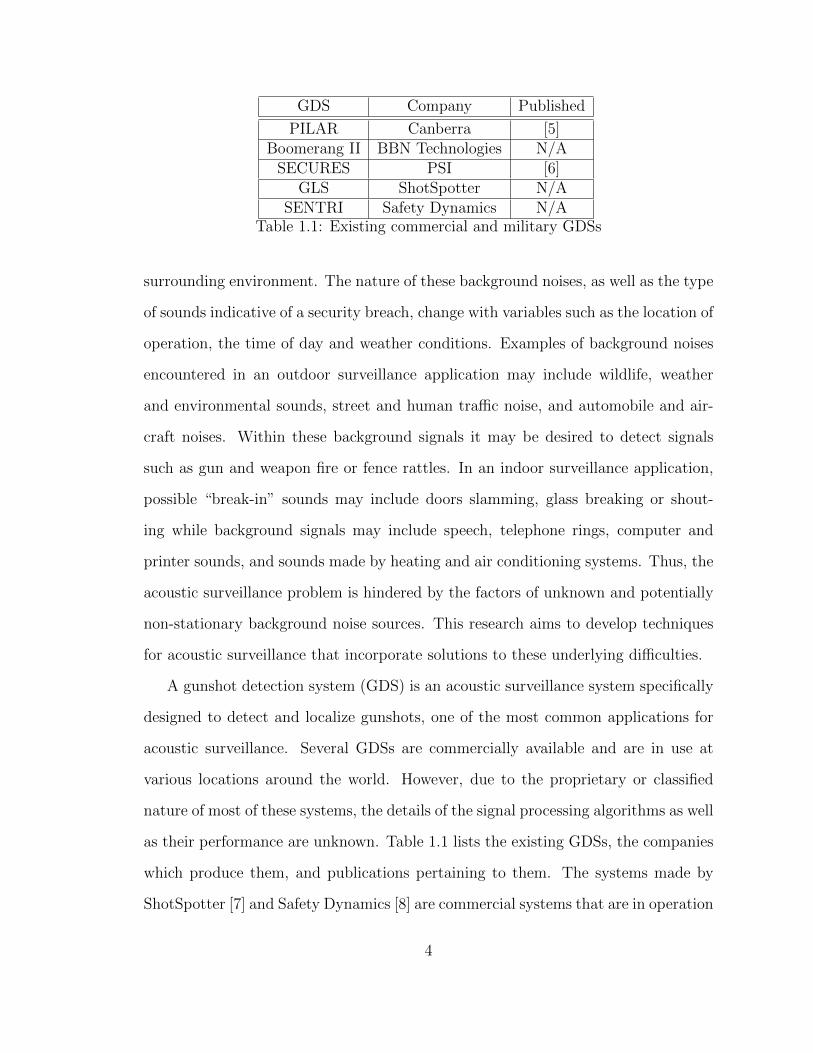
SENTRI Safety Dynamics N/ATable 1.1: Existing commercial and military GDSs

surrounding environment. The nature of these background noises, as well as the type

of sounds indicative of a security breach, change with variables such as the location of

operation, the time of day and weather conditions. Examples of background noises

encountered in an outdoor surveillance application may include wildlife, weather

and environmental sounds, street and human traffic noise, and automobile and air-

craft noises. Within these background signals it may be desired to detect signals

such as gun and weapon fire or fence rattles. In an indoor surveillance application,

possible “break-in” sounds may include doors slamming, glass breaking or shout-

ing while background signals may include speech, telephone rings, computer and

printer sounds, and sounds made by heating and air conditioning systems. Thus, the

acoustic surveillance problem is hindered by the factors of unknown and potentially

non-stationary background noise sources. This research aims to develop techniques

for acoustic surveillance that incorporate solutions to these underlying difficulties.

A gunshot detection system (GDS) is an acoustic surveillance system specifically

designed to detect and localize gunshots, one of the most common applications for

acoustic surveillance. Several GDSs are commercially available and are in use at

various locations around the world. However, due to the proprietary or classified

nature of most of these systems, the details of the signal processing algorithms as well

as their performance are unknown. Table 1.1 lists the existing GDSs, the companies

which produce them, and publications pertaining to them. The systems made by

ShotSpotter [7] and Safety Dynamics [8] are commercial systems that are in operation

4

in several cities around the United States, while the system manufactured by BBN

technologies [9] is a vehicle-mounted system currently in use in United States military

operations around the world.

GDSs can be categorized into two types of systems: those with a single platform

of sensors and those consisting of a network of sensors. Single platform systems,

such as the PILAR system [10] and the Boomerang II, contain a collection of closely

spaced microphones and computational power to perform signal processing and to

transmit detection results. Sensor network based GDSs, such as the systems from

ShotSpotter and Saftey Dynamics, contain a number of widely spaced single platform

systems which communicate detection results to a central processing location which

then fuses the results of the sensors in order to make a global decision. A single

platform system has the advantage of being portable, which allows the system to be

vehicle-mounted; whereas a sensor network based system has the ability to achieve

better performance through decision fusion. This research is focused specifically on

the detection of gunshots, a task common to both types of GDSs.

When a gun is fired, two acoustic signals are produced. As the bullet is propelled

from the muzzle of the gun it travels faster than the speed of sound. As a result, an

acoustic shock wave is produced [11]. This shock wave travels away from the bullet

as the bullet travels through the air. A second acoustic signal known as the muzzle

blast is produced as gas is released from muzzle of the gun due to the explosion of

the gunpowder. The muzzle blast is the acoustic signal one typically associates with

the sound of a gunshot. At least one of the commercially available GDSs makes use

of both the muzzle blast and the shock wave produced by the gunshot [5], and it is

hypothesized that most of the other existing systems also make use of both acoustic

signals.

Detection performance when making use of the shock wave is often much higher

than detection using only the muzzle blast as few commonly occurring acoustic events

5

produce a shock wave, and thus there is a relatively high signal to noise ratio. There

are, however, several factors which limit the efficacy of gunshot detection through

the shock wave. The duration of a shock wave produced by a typical gunshot is

approximately 200µs, and it has been found that a fairly high sampling rate, greater

than 48kHz, is required to fully capture this signal [11]. More importantly, some

types of firearms do not propel bullets at speeds above the speed of sound, and

as a result, no shock waves are created. In this case, detection of gunshots must

be accomplished entirely through the detection of the muzzle blast. These factors

indicate that detection of gunshots through the muzzle blast is one area where better

signal processing algorithms will have the ability to make a greater impact in overall

GDS performance. Thus, this work is focused toward this goal.

1.2 Acoustic Signal Detection and Classification

Detection of gunshots from muzzle blasts is a task which can be compared to a

general acoustic detection task in which the signals from a class of acoustic source

are to be detected within background signals or differentiated from other acoustic

signals. Several approaches have been developed for automated sound detection

[12, 13, 14, 15, 16, 17], two of which focus specifically on the detection of gunshots,

[16] and [17]. All of these approaches are similar in that they employ pattern clas-

sification techniques that are applied to a set of extracted features. Although the

features and classifiers differ across the approaches, the underlying ideology behind

each of the techniques is the same. A stream of time series data is partitioned into

short frames ranging between 20ms and 1s in duration. A decision regarding the

presence of the signal of interest is made in each frame via classification of a vector

of features calculated from the frame of data. The features calculated in these ap-

proaches include energy, maximum power, spectral features such as autoregressive

weights, and perceptual features such as mel-frequency cepstral coefficients. Several

6

different pattern classification techniques are used across these automated sound de-

tection approaches. These include Gaussian mixture models, hidden Markov models,

support vector machines, and hierarchical linear classifiers.

Detection results vary across these classification based approaches to acoustic

detection but in general, high detection rates and low false alarm rates are obtained

in quiet conditions. Several of these studies indicate difficulty when the signals of

interest are present within background signals, a situation likely to be encountered

in “real-world” applications such as gunshot detection [13, 12, 16]. These difficulties

in the presence of background signals could be due to the non-stationary nature of

the background signals.

Since each frame of data contains background signals as well as a possible signal

of interest, the features calculated in a particular frame will be a function of both the

background and target signals. As mentioned previously, in many acoustic detection

tasks such as muzzle blast detection, it is likely that background signals will differ

with changes in the environment due to the time of day and weather conditions.

For a feature-based classification technique to function reliably in these conditions,

a separate classifier would need to be trained for each type of background signal

encountered. In lieu of the potentially difficult and ill-defined task of selecting a

different classifier for use in different environmental conditions, reliable detection

of acoustic signals embedded within non-stationary background signals requires a

different approach to the detection task.

Although frame based approaches to acoustic signal detection have often shown

promise, each approach’s reliance on application-specific features means that the

resulting algorithms are highly application specific and difficult to generalize to other

problems of interest in acoustic sensing. A generalized model for acoustic signals

could lead to algorithms that offer reliable performance without the need for operator

or even automated selection of the appropriate features. The ability to model acoustic

7

signals without the need for signal specific tuning is also vital to an algorithm’s ability

to adapt as system requirements change over time.

1.3 Overview of this Work

This research proposes a new technique for the detection of muzzle blasts and ulti-

mately other signals of interest embedded within background signals. The approach

is based on a two stage system in which anomalous signals are detected from within

the non-stationary background signals and subsequently each anomalous signal is

further analyzed to determined if it is one of the specific signal types of interest.

This approach to signal detection allows for the characterization of the time-varying

background signals independent of the specific type of signal to be detected and the

methodology used to detect them. This approach also has the potential to signifi-

cantly reduce computational demand as the second stage of processing need only be

applied once a detection has been made by the first stage.

The environmental conditions and algorithmic requirements of a fielded acoustic

sensing system are likely to change as a function of time, location and system use. To

achieve optimal performance, algorithms for acoustic sensing must be able to adapt

to these changes. For example, consider a mobile GDS, expected to detect all types

of gunfire, mounted on a military vehicle. As the vehicle encounters enemy fire, not

only will the nature of the background noise vary due to changing environmental

conditions but also the frequency of particular types of gunshots will change depend-

ing on the types of enemy firearms in use. It may therefore be advantageous to have

an algorithm that is capable of adapting to both changing noise conditions as well

as changing target frequency within the general class of targets. These two types of

adaptation are primary motivating factors which determine the methodology used in

this research and are addressed in a principled manner through the use of Bayesian

statistical inference.

8

Probability theory, specifically its Bayesian interpretation, is the only consistent

and rational methodology for representing knowledge and thus uncertainty using

numbers [18]. Therefore, it follows that computational algorithms for detection and

estimation derived from a Bayesian perspective can be considered optimal given their

assumptions. Despite this mathematical and philosophical optimality there are sig-

nificant considerations when utilizing Bayesian inference. Firstly, the structure of the

probabilistic model, indicative of the assumptions regarding the problem, should be

designed using the available knowledge regarding the problem and no more. Char-

acterizing this available knowledge and including it in model design is one of the

difficulties of implementing a Bayesian approach. A fundamental aspect of proba-

bilistic model design is the size and thus the complexity of the model: the model

order. Recent advances in probability theory have enabled probabilistic models that

are capable of performing automated model order selection for certain probabilistic

model structures. Utilization of probabilistic models based on the Dirichlet pro-

cess (DP) [19], is fundamental to the approach used in this research to construct

probabilistic models with only the necessary complexity.

Also of fundamental importance to algorithms making use of probabilistic models

is the methodology used to conduct inference. Bayesian inference for most interesting

probabilistic models requires some form of approximation to determine the posterior

density of the parameters. There are many methods for approximate Bayesian in-

ference each with differing trade-offs between the quality of the approximation, the

required computational complexity and the form of the posterior estimate. Given

the operational requirements and algorithm desiderata the variational Bayes (VB)

method along with conjugate priors are utilized within this research. Mathemati-

cal details for the probabilistic methodology in both stationary and non-stationary

environments are discussed in Chapter 2.

A Bayesian approach to the detection of anomalous signals within non-stationary

9

background signals is discussed in Chapter 3. This serves as the first stage of process-

ing of the proposed acoustic sensing algorithm, and allows the proposed algorithm to

adapt to the time varying nature of the background signals. Specifically, the approach

undertaking in this research is based on Bayesian non-stationary autoregressive (AR)

modeling of the background signals and detecting deviations in the likelihood of this

background signal model. An AR model serves as a time domain model capable

of encapsulating the spectral and intensity properties of the background signal, and

modeling the background signal as a non-stationary processes allows the background

signal model to adapt to environmental conditions. Both maximum likelihood and

Bayesian estimation of non-stationary autoregressive models are analyzed and ap-

plied to the task of gunshot detection. It is observed that Bayesian estimation

of non-stationary AR models results in a very similar algorithm to the least mean

squares (LMS) algorithm, a typically employed algorithm that results from maximum

likelihood learning. It is determined that the Bayesian approach has advantages over

an LMS based approach because more accurate estimates of the parameters can be

determined without the need to perform extraneous ad hoc processing. This results

in improved detection performance by the Bayesian approach.

Following detection in the first stage of processing, anomalous signals are distin-

guished using a statistical model, in the second stage of processing. In contrast to

the feature based approaches utilized in previous acoustic classification studies, this

research proposes the use of a statistical model that operates on the time-domain

acoustic signal and makes minimal assumptions regarding the nature of the specific

acoustic signals under consideration. In Chapters 4 and 5 a flexible statistical model

for acoustic signals is developed and analyzed while keeping in mind computational

complexity and algorithmic ability to adapt to newly acquired data. The approach

to signal modeling once again makes use of AR models as statistical models capable

of characterizing the spectral and intensity properties of a time-series but contrary to

10

the background signal model conducted in Chapter 3 more sophisticated statistical

models are necessary to model the complex spectral nature of the signals of interest.

The background signals model in Chapter 3 change with time in unforeseen ways and

as such are modeled as non-stationary processes with limited knowledge of how they

will evolve over time. The signals to be classified in the second stage of the proposed

framework are typically short duration (typically less than one second) acoustic phe-

nomenon such as a muzzle blast or a car door slam, and can be characterized by

the energy and spectral changes over their duration. Therefore, the goal in Chap-

ters 4 and 5 is to develop a statistical model for time-domain data that is capable

of characterizing multiple sets of spectral and energy properties and modeling the

occurrence of these properties. Given such a model for acoustic signals under the

hypotheses of interest, inference can be performed using optimal approaches such as

likelihood ratio tests and/or maximum a posteriori classification. The use of time

domain signal models eliminates the need to determine application-specific features

and provides straightforward methods for performing statistical inference.

As mentioned previously, a significant concern when constructing probabilistic

models is the complexity of the model, the model order. The order of an AR model

controls the spectral complexity contained within the model and has a great impact

on the model’s robustness to unseen data. To create a statistical model for time-

series data a single AR model is insufficient, therefore, this work proposes the use

of hierarchical models, such as mixture models and hidden Markov models (HMMs),

that make use of AR models. The use of hierarchical statistical models such as

mixture and hidden Markov also require model order selection to determine the

number of components in the mixture model or the number of states within the

HMM. When utilizing AR models within a larger statistical model, such as a mixture

model for example, the problems of model order selection are compounded as both the

number of elements in the mixture and the AR order within each mixture component

11

must be determined simultaneously. Although quantitative model order selection

techniques exist for selecting the AR order and the number of states within the

mixture model, these techniques quickly become computationally intractable as they

require exhaustive evaluation of each AR order and number of mixture components

combination under consideration.

In this work, a probabilistic approach is taken to the AR order estimation prob-

lem. By making use of conjugate priors, a tractable solution is offered that provides a

probability density over the available AR orders, thus providing an automated means

of determining the appropriate AR order that is computationally tractable when in-

clusioned within larger statistical models. This technique, called the uncertain-order

AR (UOAR) model is compared to standard techniques for quantitative AR order

estimation and shown to perform favorably in Chapter 4. Chapter 4 also develops

and analyzes a DP mixture of UOAR models (DP UOAR) as a flexible model for

time-series data that performs automated model order selection at both the number

of mixture components and the AR order levels. The proposed model is similar to

that considered in [20], but in this research the VB method is utilized to provide more

rapid parameter inference and a parameterized posterior distribution, both necessi-

ties for the tractable principled algorithm updating that is desired. The VB learning

procedure that has been developed is compared to more exact but more computation-

ally intensive Markov chain Monte Carlo (MCMC) approximate Bayesian inference

like that conducted in [20] and [21] and the VB learning procedure is shown to per-

form nearly as accurately as MCMC inference while providing a solution consistent

with the desired algorithm behavior. The flexible model for time-series data is then

applied to a classification task wherein acoustic signals indicative of security breach

are discriminated. It is shown that the automated order selection properties of the

DP UOAR offer performance equal to performing a very costly exhaustive search

over appropriate model orders.

12

In Chapter 5 the DP UOAR model is adapted to include a model for the time

structure of the spectral and energy properties of the signal. This is done tractably

by considering an HMM of UOAR sources. Using techniques derived from an inter-

pretation of the Dirichlet process known as stick-breaking [22] presented in [23], a

stick-breaking HMM (SBHMM) is constructed to perform automated selection of the

number of states within the HMM. Although alternate constructions for automated

state selection in HMMs have been proposed based on the hierarchical Dirichlet

process [24], the approach of [23] allows for the application of VB inference. The

derived VB learning procedure for the UOAR SBHMM then serves as a tractable,

highly flexible model for time-series data that offers automatic model order selection

in each of its parameters. Similar models of HMM with AR components have been

recently proposed in [25] and [26] but once again have only made use of MCMC

inference. The proposed model extends upon these studies by including automated

model selection of the AR order as well as conducting VB inference to maintain the

ability to update the resulting model in a principled and computationally efficient

manner.

The UOAR SBHMM, explored in Chapter 5, assumes that an acoustic signal

contains different spectral and intensity characteristics and transitions between them

over the duration of the signal. The number of different spectral and intensity char-

acteristics, the number of HMM states, is not predetermined, nor is the spectral

complexity within each HMM state, the AR order. The primary assumption made

by this model is that transitions between the spectral and intensity states follow a

Markov model, an assumption that must be made to maintain tractability. Since

this model operates on the time-series of the data and is purely generative, this work

demonstrates how this model can be used to synthetically generate acoustic signals,

an interesting aspect of the proposed methodology. The resulting model is used to

classify various types of acoustic signals and shown to perform very favorably. The

13

flexibility of the UOAR SBHMM to general time-series data is then illustrated by

applying the model to the classification of landmine responses from time-domain

ground penetrating radar. Although model development was not specifically de-

signed to characterize these types of time-series the model performs well, validating

the flexibility of our approach to time-series modeling.

The ability to characterize many types of acoustic signals with a highly flexible

model enables the classification of acoustic signals without the necessity of human

intervention into model or classifier development. However, to perform this type of

analysis, the specific types of acoustic signals to be discriminated must be known

and labeled prior to parameter inference. Often the task of concern, particularly in

acoustic surveillance, is not to identify the type of acoustic signal that was detected

but instead to sound an alarm to indicate a possible break-in in progress. Therefore,

statistical inference for this problem requires a model that groups all of the sounds

indicative of a break-in into a single hypothesis. It is inappropriate, however, to

utilize a single UOAR SBHMM to model two sounds indicative of a break-in that

may have dramatically different time-frequency characteristics, for example glass

breaking and a small explosion. An alternative would be to specifically label all

available data and develop a model for each unique label. However, there is no reason

to believe that all examples of a given assigned label, such as glass breaking, will

share common time-frequency characteristics. They may be similar but there may

be physical properties of particular glass samples or causes of breaking that result

in different time-frequency properties. As a results, a more sophisticated statistical

model is required that can model signals with different time-frequency properties

and automatically group these signals appropriately.

Appropriate selection of this statistical model can also create an algorithm capa-

ble of adapting to the frequency of specific types of signals within the class of interest

and even learn previously unseen classes of data. Consider again the example of a

14

vehicle-mounted GDS. Each type of firearm causes a slightly different muzzle blast

due to the physical characteristics of the gun and therefore is more appropriately

modeled by a different UOAR SBHMM. Within the larger statistical model for all

types of muzzle blasts the likelihood of specific muzzle blasts can be modified given

the recent observations of the GDS. Furthermore, the signal model for a newly ac-

quired muzzle blasts can be updated based on new observations. Similarly, if a new

type of firearm is encountered by the GDS and it causes a muzzle blast with time-

frequency properties different from anything previously seen by the system, this new

type of signal should be automatically modeled by the system.

A statistical model capable of these types of adaption is presented in Chapter 6

wherein a DP mixture of UOAR SBHMMs is developed. The model jointly clusters

time-series based on their time-frequency characteristics and models each cluster

using an UOAR SBHMM, and due to the DP nature of the model, the number

of clusters is automatically estimated from the data. The resulting model then

only requires that sounds of interest be separated from those not of interest and

a hierarchical model can be learned for each of the two hypotheses. Once again

a VB learning procedure is developed to provide rapid parameter inference with

a parameterized posterior density. This allows the algorithm to update the current

posterior density when, for example, a muzzle blast is correctly detected and feedback

is given to the system, the likelihood of observing a muzzle blast from this particular

type of firearm should increase in the newly updated model. The use of this model

for detection of a class of acoustic signals is then presented along with analysis of the

clustering determined by the algorithm. The ability of the model to adapt to newly

acquired data is then illustrated using an example scenario similar to the discussed

mobile GDS example. The ability of the algorithm to adapt in this principled and

tractable manner is a validation of the choice of VB inference.

The DP mixture of UOAR SBHMMs model for time-series modeling is similar

15

to the DP mixture of HMMs that is considered in [27, 28, 29] for the purposes of

music analysis. There are several notable distinctions between this work and that

presented in these previous studies. First, a SBHMM is considered here as the

base density within the mixture thus eliminating the need to specify the number of

states within the HMM for each cluster. Second, in this work it is assumed that

each acoustic signal is generated by a single HMM, which is consistent with our

model for relatively short duration acoustic signals, whereas in [27, 28, 29] each

time sample can be generated a different HMM, an assumption more appropriate for

music analysis. Most important, however, is that the proposed model makes use of

the UOAR model within each state of each HMM thus operating directly on the time

domain data and maintaining consistency with our previously discussed time-series

models. This is contrary to [27, 28, 29] where the data is transformed into a series of

mel-frequency cepstral coefficients, an application specific feature set. The proposed

DP mixture of UOAR SBHMMs thus remains a highly flexible model that makes

limited assumptions regarding the types of time-series that it operates on.

The methods presented in this work represent a Bayesian approach to acoustic

surveillance that remains independent of the specific types of acoustic signals un-

der consideration. The use of the VB method and conjugate priors for approximate

Bayesian inference leads to computationally tractable algorithms that are amenable

to updating to newly acquired data. The methodology creates an acoustic surveil-

lance framework that is able to adapt to its surroundings to improve performance.

The proposed formulation, when applied to acoustic gunshot detection, serves as a

compliment to shockwave based detection algorithms and the decisions made by each

may be combined to improve performance or to detect gunfire that does not produce

muzzle blasts. As illustrated by the application to time-domain radar landmine re-

sponses the proposed model for time-series data is very flexible and has applications

outside of acoustic signals. In addition the model may be applicable for use within

16

other statistical models that may be used to solve outstanding problems in acoustic

sensing such as convolutive source separation. These conclusions and discussions of

directions for future work are discussed in Chapter 7.

17

2

Background

The primary goal of this research is to develop acoustic sensing algorithms that are

capable of adapting to changes in operating conditions as a means of improving sys-

tem performance. To provide a principled yet tractable approach to algorithm adap-

tation, the problem is approached using probabilistic models and Bayesian inference.

Under a Bayesian framework, parameters are not estimated, but instead knowledge of

the parameters is measured using probability theory and when new data is acquired

knowledge of the parameters is adjusted in a principled manner. The use of Bayesian

inference also enables estimation of probabilistic model structures that perform au-

tomated model order selection, a necessity for robust, application-independent sta-

tistical models for acoustic signals. Models of this type will be explored in Chapters

4, 5 and 6. This chapter presents an overview of Bayesian parameter estimation

techniques, specifically conjugate priors and the variational Bayes method. When

coupled with conjugate priors, the variational Bayes method is a computationally

tractable solution for approximate Bayesian inference that is amenable to recursive

estimation and on-line learning.

18

2.1 Bayesian Parameter Estimation

Often in signal processing applications, the tasks of interest are the detection and

classification of signals of interest within observed data. Approaching both of these

tasks from a statistical point of view often leads to learning the parameters of a

generative model. The resulting statistical models for the observed data under each

hypothesis can then be used to form the likelihood ratio test to detect signals or

perform classification. In this research it is assumed that a set of data is comprised

of T samples that are denoted as D = [d1, d2, . . . , dT ]′. The parameterized genera-

tive statistical model for the data is defined in terms of the conditional probability

density for the data set given the parameters, f (D|θ), where the set of n parameters

are denoted as θ = [θ1, θ2, ..., θn]′. Given the set of data D, it is the goal of statis-

tical learning to acquire information about the of set parameters, θ. The resulting

learned parameters can then be used to make inferences regarding detection and

classification.

In many applications merely finding estimates of the parameters, θ, is sufficient.

Typically, these estimates are chosen to maximize the likelihood of the parame-

ters, L (θ) = f (D|θ), or to maximize the a posteriori density of the parameters,

f (θ|D) ∝ f (D|θ) f (θ), yielding ML estimates and MAP estimates respectively. In

some applications, however, it is desirable to learn a full posterior density for the

parameters. A full posterior density for the parameters can be used to measure the

underlying uncertainty in the estimates of the parameters and thus aid statistical

inference. Bayesian parameter estimation seeks to find the posterior density of the

parameters given the set of data and some prior information of the parameters, f (θ).

The posterior is formulated using Bayes’ rule.

f (θ|D) =f (D|θ) f (θ)

f (D)(2.1)

19

The denominator of (2.1), f (D), is the marginal likelihood of the dataset and is often

called the evidence. Calculating the evidence requires integrating the joint density

of the data and parameters.

f (D) =

∫f (D, θ) dθ =

∫f (D|θ) f (θ) dθ (2.2)

The evidence is the normalizing constant for the posterior density and due to the

potentially high dimensional integration in (2.2), it is often difficult to obtain. For

this reason, approximations to the posterior parameter density are often necessary.

Point estimates, such as ML and MAP estimates, approximate the posterior param-

eter density as a Dirac delta function. This type of posterior parameter estimate is

known as a certainty equivalent approximation [30].

f (θ|D) = δ(θ − θ

)(2.3)

Due to their simplicity, certainty equivalents are the most common method of

parameter estimation, however, such estimates ignore all of the true uncertainty as-

sociated with the estimates of the parameters. In comparison, modeling the posterior

of the parameters with a more appropriate probability density function allows the

incorporation of the true underlying uncertainty in these parameters, θ. Approxi-

mating the posterior density, however, can be computationally expensive, so reaching

a compromise between the quality of the approximation and the computational cost

is necessary.

A variety of methods, collectively referred to as Markov chain Monte Carlo

(MCMC) methods [31], approximate the posterior density through numerical sam-

pling. This leads to an approximate density of the form

f (θ|D) =1

N

N∑i=1

δ(θ − θ(i)

). (2.4)

20

Forming a posterior density of this form requires a set of θ(i) that are drawn from

the true posterior density. Many different algorithms for MCMC sampling exist,

each with trade-offs between assumptions and computational complexity. In general,

however, MCMC sampling enables estimation of the posterior density for nearly any

statistical model. Algorithmically, MCMC inference draws samples from the pos-

terior density by iteratively drawing samples of each parameter conditioned on the

previously drawn parameters on which they depend. This creates a Markov chain of

sampling that eventually reaches a steady state at the posterior density. The number

of samples to reach this steady state, the burn in rate, is difficult to quantify, as is

the number of samples, N , required to obtain an adequate estimate of the posterior

density. Conservative selection of these parameters, however, allows a posterior den-

sity to be approximated to any desired accuracy with increasing computational costs

and as a result, MCMC methods have been established as the standard by which

other approximation methods can be compared [32]. However, the non-parametric

form of the posteriors acquired by sampling methods contributes to additional com-

putational costs when they are used for statistical inference beyond the calculation

of the posterior such as that required for recursive Bayesian learning.

An alternative method for approximate Bayesian inference known as the Lapla-

cian approximation approximates the posterior density as a multivariate Normal

distribution [33]. The mean of the posterior density is the MAP estimate of the

parameter means and the covariance matrix is assumed to be the negative of the

inverse of the Hessian of the logarithm of the joint distribution of the parameters

and the dataset with respect to the parameters, evaluated at the MAP estimate of

the parameters.

f (θ|D) = N(θMAP , H

−1)

(2.5)

21

Hij = − ∂2

∂θi∂θjlog f (θ,D)

∣∣∣θ=θMAP

(2.6)

The Laplacian approximation provides a full posterior density by assuming a known

functional form with a mean equal to the MAP estimate. However, calculation of

the covariance matrix requires inversion of the Hessian matrix (2.6). When there

are a large number of parameters, and a full posterior density is most beneficial,

the inversion of the Hessian matrix may be unstable as well as computationally

intractable. There may also be circumstances where assuming the a multivariate

normal over the posterior is inappropriate due to physical or statistical constraints

on the parameters. For example, this would be an inappropriate model when some

parameters are known to be strictly positive.

Another approach to approximate Bayesian inference, known as moment match-

ing approximations, attempts to fit the parameters of specified moments of posterior

density to create a posterior density with a known functional form. Moment match-

ing yields a smooth parameterized estimate of the posterior distribution, however, the

require optimization may be intractable for certain observation models and moment

choices. Furthermore, there is no specified way to select the number of moments that

should be estimated. These parameters must be selected on an application specific

basis.

Although each of these methods approximates the posterior density while bal-

ancing the quality of the approximation with the computational costs associated

with it, each method has limitations under certain conditions. Recall that the use of

Bayesian parameter estimation in this research is focused on the estimation of the pa-

rameters of statistical models for acoustic sensing and creating algorithms that have

a principled mechanism for adapting to changing operating conditions. Algorithmic

adaption can be accomplished utilizing recursive Bayesian inference wherein the pos-

terior density at time t is used as the prior density at time t+1. The approximations

22

discussed thus far do not provide a tractable solution to this problem.

2.1.1 The Conjugate Prior Approximation

For a given observation model for dataset D, f (D|θ), there may exist a prior dis-

tribution for the parameters, f (θ), with a functional form which yields a posterior

distribution of the same functional form. If the prior distribution were defined by

parameters, λ0, known as the hyper-parameters, the parameters of the posterior dis-

tribution would be defined by a functional mapping of the prior hyper-parameters

and the dataset, λ1 = U (λ0, D). Under these circumstances the prior density is

said to be the conjugate prior (CP) for the observation model [34]. Further insight

into CPs can be gained if the form of the observation model under consideration is

restricted to a family of distributions.

Most common distributions belong to the exponential family of distributions [35].

These distributions include the normal distribution, the multinomial distribution,

the Poisson distribution, the gamma distribution, the Dirichlet distribution and the

Wishart distribution, amongst others. These statistical distributions have probability

density functions of the following form.

f (D|θ) = ev(θ)′u(D)+log h(D)+log g(θ) (2.7)

In (2.7), v (θ) is a vector of functions of the parameters, u (D) is a vector of functions

of the dataset, and h (D) and g (θ) are normalizing constants that are functions of

the dataset and the parameters respectively. The CP for density functions of this

form is defined by hyper-parameters λ = ν,V.

f (θ) = ev(θ)′V+ν log g(θ)+log z(ν,V) (2.8)

Here, z (ν,V) is a normalizing constant that is a function of the hyper-parameters.

The conjugacy of the prior with the observation model ensures that the posterior

23

density has the same functional form as 2.8. For a particular observation model and

CP, the update functions for the hyper-parameters must be determined. For many

common observation model and CP pairs, the hyper-parameter update functions are

well known and are computationally simple [34].

Limiting the functional form of the prior and posterior distributions of the param-

eters for a particular observation model may be viewed as an approximation method

that can be compared to those discussed in Section 2.1. Contrary to the approxima-

tion methods previously discussed, the calculation of the posterior parameter density

using the CP approximation provides the exact solution given the assumptions on the

functional form of the prior and the observation model. These assumptions about the

form of the prior, and thus posterior, can be viewed as an approximation. This is a

key difference between the CP approximation and the other approximation methods

discussed in Section 2.1. The quality of the CP approximation is difficult to quantize

in general and must be handled on an application specific basis.

In on-line applications the entire dataset is not received at one time but sequen-

tially in smaller pieces. The CP approximation is initialized with a prior distribution

which is conjugate to the observation model. This prior distribution is specified by

the hyper-parameters, λ0. Some initial dataset is observed at time t and is denoted

Dt. For this example it is assumed that the observation model and CP yield a set

of hyper-parameter update equations denoted by U (·, ·). From this initial dataset

and set of update equations, the posterior density estimate can be determined by

updating hyper-parameters, λt = U (λ0, Dt).

When an additional dataset is received at a later time t+ 1 (Dt+1) the previous

posterior estimate can be used as the prior and a new posterior can be determined.

λt+1 = U (λt, Dt+1) (2.9)

As mentioned above, sequential updating can be performed without retaining any of

24

the previous datasets, rather, only the updated hyper-parameters that resulted from

the previous datasets need to be retained. This prior-posterior-prior process can

be repeated as additional data is observed with very little additional computational

costs with the only approximation imposed by the choice of the prior and thus the

posterior.

The CP approximation method can provide posterior density estimates in on-line

scenarios with very little additional computational costs. This simplicity in on-line

scenarios highlights one of the main strengths of the CP approximation. For some

statistical models, however, particularly those with latent or hidden variables, con-

jugate priors are unattainable. As will be demonstrated in Chapters 4 and 5, a

statistical model that is capable of characterizing acoustic signals requires sophisti-

cated structure and hidden variables. Therefore, an alternate form of approximate

Bayesian inference is required. Furthermore, in this work it is required that the ap-

proximate Bayesian inference technique is amenable to recursive Bayesian inference,

allowing for algorithm adaptation.

2.1.2 Bayesian Parameter Estimation with Hidden Variables

Consider now an observation model for dataset D, which is dependent on hidden

variables s and a set of parameters θ. Typical examples of models of this type include

mixture models and hidden Markov models (HMMs). In the case of a mixture model,

the hidden variables indicate underlying membership in a mixture component, or in

the case of an HMM they indicate an underlying state. The parameters, θ, can

be decomposed into two subsets of parameters, θ = θD, θs, where θD is the set of

parameters that govern the observation model given the hidden variables, f (D|s, θD),

and θs are the parameters that determine the density of the hidden variables, f (s|θs).

Bayesian parameter estimation under this paradigm seeks the density of all of the

25

parameters, θ, given the observed data, D, and the unobserved hidden variables, s.

f (θ|D, s) =f (D|s, θD) f (s|θs) f (θ)

f (D, s)(2.10)

The evidence in this case is the joint density of the data and the hidden variables.

f (D, s) =

∫f (D|s, θD) f (s|θs) f (θ) dθ (2.11)

As before, the integration required to calculate the evidence, in most cases, is

intractable and as a result, the problem is often reformulated and point estimates of

the parameters are found. Maximum likelihood (or maximum a posterior) parameter

estimates, θ, can be found using the EM algorithm [36]. In general, CPs cannot

be found in the presence of hidden variables and as a result, Bayesian parameter

estimation requires approximation. One form of approximation which allows for

application in on-line scenarios makes use of a variational method that was introduced

in statistical physics [37], known as variational Bayes (VB).

2.2 Variational Bayesian Learning

2.2.1 Variational Methods

Variational methods aim to approximate a complicated integral by instead maximiz-

ing a lower bound of an approximation of the integral. By approximating an integral

by maximizing a lower bound, the intractable integral is transformed to a tractable

optimization problem. Consider a function, g (x). The goal is to determine G, the

integral of g over all x.

G =

∫g (x) dx (2.12)

In many problems, x is very high dimensional and analytical calculation of this

integral is intractable. The variational approximation to the integral is formed by

26

choosing a function, q, which is a function of x and ε, the variational parameters.

The form of q is chosen such that the integral is tractable and the bounded from

below. The integral is then approximated by Q (ε).

G ≥ Q (ε) =

∫q (x, ε) dx (2.13)

The integral can then be approximated by maximizing Q (ε) with respect to the

variational parameters, thus turning the integration problem into an optimization

problem.

2.2.2 Variational Bayes

Variational Bayes is a variational technique to approximate a probability density

function when the required integration is intractable (e.g. [38, 39, 30, 40, 41, 42]).

It is assumed that the entire collection of parameters is denoted θ. The variational

approximation of the posterior of the parameters is denoted q (θ) wherein the condi-

tioning of the posterior density upon the dataset is implied.

f (θ|D) = q (θ) (2.14)

The functional form of the approximate posterior densities must be determined to

make the integral (in (2.2) or (2.11)) tractable and then optimized with respect to

the hyper-parameters. To understand how the variational approximation should be

optimized it is helpful to view the evidence in a form different than that given in

(2.2).

f (D) =f (D, θ)

f (θ|D)(2.15)

Calculation of the evidence in this manner requires calculation of the true posterior

distribution, which is unattainable. By manipulating the log-evidence, the varia-

tional posterior approximation can be used to formulate the calculation of the evi-

27

dence as an optimization problem.

log f (D) = logf (D, θ)

f (θ|D)(2.16)

= logf (D, θ) q (θ)

f (θ|D) q (θ)(2.17)

=

∫q (θ) log

f (D, θ) q (θ)

f (θ|D) q (θ)dθ (2.18)

=

∫q (θ) log

f (D, θ)

q (θ)dθ +

∫q (θ) log

q (θ)

f (θ|D)dθ (2.19)

= F (q (θ)) + KL (q (θ) ||f (θ|D)) (2.20)

The first term of (2.20) is known as the negative free energy and is defined as

F (q (θ)) =

∫q (θ) log

f (D, θ)

q (θ)dθ. (2.21)

The second term of (2.20) is the Kullback-Liebler divergence (KLD) between the

variational approximate posterior and the true posterior, an unattainable term. The

KLD is a measure of similarity between two probability distributions. Noting that

the KLD between any two probability density functions is always positive, (2.20) can

be rearranged to show that the negative free energy forms a lower bound on the true

log-evidence.

F (q (θ)) = log f (D)−KL (q (θ) ||f (θ|D)) (2.22)

The negative free energy can thus be used to optimize the approximation posterior

since maximizing the negative free energy with respect to the parameters of the

approximate posterior density is equivalent to minimizing the distance between the

true and the approximate posteriors.

The KLD between any two probability density functions is minimized (i.e. is

identically zero) when the two probability density functions are identical. This leads

to the trivial solution that the optimal variational approximation is achieved when

28

q (θ) = f (θ|D). Despite the fact that f (θ|D) is unattainable, the negative free

energy can be maximized with respect to q (θ) by assuming that the parameters can

be partitioned into groups that are conditionally independent given the observed

data. If these groups are denoted as θi for 1 ≤ i ≤ k the approximate posterior

density is

q (θ) =k∏i=1

q (θi) . (2.23)

Using this independence assumption the approximate posterior density can be par-

titioned as the product of the approximate posterior for specific parameter group,

q (θi), and all other parameter groups, q (θ−i)

q (θ−i) =n∏j=1j 6=i

q (θj) . (2.24)

Using (2.24), the posterior density which maximizes the negative free energy, 2.21,

with respect to θi is derived as follows. Similar derivations can be found in [30, 43,

44, 45]. The derivation presented here is most similar to that in [30].

F (q (θ)) = log f (D)−KL (q (θ) ||f (θ|D)) . (2.25)

= log f (D)−∫q (θ) log

q (θ) f (D)

f (θ|D) f (D)dθ (2.26)

= log f (D)−∫q (θ) log q (θ) dθ − log f (D)

−∫q (θ) log f (θ,D) dθ (2.27)

Using the separation of θi from θ−i and then defining H (·) as the entropy operator

29

for probability density functions, defined in the Appendix B, yields the following.

F (q (θ)) = −∫q (θ) log q (θi) dθ −

∫q (θ) log q (θ−i) dθ

+

∫q (θi)

[∫q (θ−i) log f (θ,D) dθ−i

]dθi (2.28)

= −∫q (θi) log q (θi) dθi −H (q (θ−i))

+

∫q (θi)

[Eq(θ−i)log f (θ,D)

]dθi (2.29)

Introducing the term Z (θ−i), defined as

Z (θ−i) =

∫expEq(θ−i)log f (θ,D)dθ−i. (2.30)

the derivation continues by adding and subtracting this term inside the integral of

the second term.

F (q (θ)) = −∫q (θi) log q (θi) dθi −H (q (θ−i))

+

∫q (θi)

[logZ (θ−i)− logZ (θ−i) + log expEq(θ−i)log f (θ,D)

]dθi

(2.31)

= −∫q (θi) log q (θi) dθi −H (q (θ−i))

+

∫q (θi) log

1

Z (θ−i)expEq(θ−i)log f (θ,D)dθi + logZ (θ−i) (2.32)

Combining the integrals over θi,

F (q (θ)) = logZ (θ−i)−H (q (θ−i)) +

−∫q (θi) log

q (θi)1

Z(θ−i)expEq(θ−i)log f (θ,D)

dθi (2.33)

= logZ (θ−i)−H (q (θ−i))

−KL

(q (θi) ||

1

Z (θ−i)expEq(θ−i)log f (θ,D)

). (2.34)

30

In (2.34) the only term dependent on θi is the KLD term. Maximizing the negative

free energy with respect to any individual θi can thus be done by minimizing this

term. Noting again that the KLD is minimized when there is equality between the

two probability density functions, the variational approximate for parameter θi which

maximizes the negative free energy is

log q (θi) ∝ Eq(θ−i)log f (D, θ). (2.35)

This quantity is known as the variational approximate marginal density for θi.

As seen in (2.35), the solution for each variational approximate posterior is defined

in terms of the other parameters and as a result it is unlikely that this system of

equations can be solved analytically. Instead they can be solved using coordinate

ascent, similar to EM [30]. Solving these equations in this way is known as the

variational Bayesian method. To solve a set of coupled equations using coordinate

ascent, the variational approximate for each variable must be determined by using

the current estimates of the other variational approximates. After the density for

each parameter has been updated an iteration of the algorithm has been completed.

Following each iteration, the negative free energy can be calculated and it can be

shown that each iteration of coordinate ascent is guaranteed to increase the negative

free energy or leave it unchanged [46]. Convergence of the algorithm is reached when

the change in negative free energy between iterations is negligible. This quantitative

method to determine convergence is one of the major advantages of the VB method

and is in sharp contrast to MCMC based inference.

Calculation of the negative free energy is made more convenient if the numerator

of the logarithm in (2.21) is written as f (D|θ) f (θ) and the result is simplified to

F (q (θ)) = Eq(θ)log f (D|θ) −KL (q (θ) ||f (θ)) . (2.36)

Notice now that the expected value in the first term is taken over all parameters,

this term is known as the variational average log likelihood. The second term is the

31

KLD between the approximate posterior density and the prior density, both available

quantities. The negative free energy can be calculated using (2.36) at the end of each

iteration of the VB method to monitor convergence. The two terms in (2.36) also

provide insight into the inner workings of the VB method. Because the VB method

maximize the negative free energy and the KLD is always positive, the algorithm thus

balances a trade off between the two terms. The average log likelihood measures the

fit of the model while the KLD term penalizes adjusting posterior densities to be

different from the prior. (Therefore, illustrating the principle commonly known as

Occam’s razor.) Bayesian inference, and thus the VB method, favors models that are

as simple as necessary to explain the data. This is clearly illustrated by this view of

the negative free energy. The ability of Bayesian inference to control the complexity

of the inferred model is a analyzed more closely in Chapters 4, 5 and 6 when models

for acoustic sensing tasks are developed.

Because of the iterative nature of the VB method, it is sometimes referred to as

Variational Bayes Expectation Maximization (VBEM) due to its similarity to the

EM algorithm. In fact, VB is actually a generalization of EM [31]. It can be seen

that the variational approximation for parameter group θi reduces to the expectation

of the other parameters when

q (θ−i) =n∏j=1j 6=i

δ(θj − θj

). (2.37)

log q (θi) ∝ Eq(θ−i)log f (D, θ) = log f(D, θi|θ−i = θ−i

)(2.38)

This occurs when using a certainty equivalent posterior approximation such as ML

or MAP estimates as is done in the EM algorithm.

It is interesting to note that until this point the functional form of the posterior

approximates have yet to be defined. For this reason the VB approximation is known

32

as a free-form approximation. This is a notable difference from the Laplacian and

moment matching approximations, where the functional form of the approximate

posterior is defined a priori. At the same time, the VB approximation is deter-

ministic; a clear distinction from stochastic approximation methods such as MCMC

methods.

As can be seen in (2.35), the functional form of the variational approximate

posterior density is determined by the functional form of the prior density, f (θ). To

make the VB approximation computationally tractable, the variational approximate

priors are typically chosen to be known functional forms and often they are conjugate

prior densities for the conditional form of the observation model. Choosing the prior

densities to be CPs to f (D|s, θ) yields posterior densities, f (θ|D, s) which have the

same functional form as f (θ). This allows the VB method to gain the same benefits

in on-line applications as the CPs approximation, as discussed in Section 2.1.1. This

will be exploited in Chapter 6 when a model for a collection of acoustic signals of

interest is developed and recursively updated.

Using known functional forms for the prior densities also simplifies the calculation

of the variational approximate marginals required to perform the iterative variational

Bayes algorithm, (2.35). Calculating the variational approximate marginals requires

finding the expected value of the log of the joint density of the observation model and

the parameters, f (θ,D). Calculating this expected value often requires calculating

the expected value of functional mappings of some parameters. These are sometimes

known as the variational moments.

Using CP functional forms can also help to enforce statistical constraints which

are required for some parameters. For example, consider a multivariate normal

observation model with a known mean, µ, and unknown covariance matrix, Σ. The

CP for the covariance matrix is the inverse-Wishart density which is defined by

scalar, η, and matrix, S [47, 30] (also see Appendix A). The inverse-Wishart density

33

inherently enforces that the covariance matrix is positive definite. A different choice

for the prior may not ensure that draws from the posterior density will be proper

covariance matrices. To extend the example, consider an observation model with

more parameters, θ, one of which is the covariance matrix, θj = Σ. To estimate the

posterior density of another one of the parameters, θi, under the variational Bayes

paradigm it will be necessary to take the expected value of the observation model

over Σ. This may require an integration such as

Eq(Σ)log|Σ| =

∫Σ

log|Σ|q (Σ) dΣ, (2.39)

where again q (Σ) is our variational posterior approximate. This expected value

requires integration over all possible positive semi-definite matrices. For most choices

of the functional form of q (Σ) this integral is intractable. However, using the inverse-

Wishart density for Σ results in an analytic solution to this integral, namely,

EΣlog|Σ| = −d log 2−d∑i=1

Ψ

(η − i+ 1

2

)+ log|S|, (2.40)

where d is the dimensionality of the covariance matrix and Ψ (·) is the digamma

function (see Appendix B).

In summary, VB maximizes a lower-bound on the approximation of a multi-

dimensional probability distribution by minimizing the KLD between the approxi-

mate and the true distribution. The resulting inference algorithm takes the form of

a coupled set of equations that are solved through coordinate ascent. When coupled

with CPs, the VB method provides a computationally tractable solution for Bayesian

inference of sophisticated statistical models and yields a posterior density that is of

the same functional form as the prior. This makes the VB method an appropriate

choice when recursive Bayesian inference is required. The VB method will be used

in Chapters 4 and 5 to determine the posterior density for the parameters of mod-

34

els for acoustic signals and in Chapter 6 to determine the posterior density for the

parameters of a model for a collection of acoustic signals. The ability to perform

recursive Bayesian inference using posterior densities obtained from the VB method,

is utilized in Chapter 6, when the model for a collection of acoustic signals is updated

as new signals are obtained.

2.3 Bayesian Estimation of Non-Stationary Parameters

As mentioned previously, Bayesian parameter estimation with the VB method and

CP can be easily extended to on-line situations, through tractable recursive Bayesian

inference. When the underlying statistics are stationary (constant as a function

of time), as more data is received the entropy of posterior parameter densities is

decreased. This indicates an increase in the “confidence” of the estimate of the

parameters. However Bayesian parameter estimation of a non-stationary processes

is a significantly more complicated task.

The discussion of non-stationary Bayesian parameter estimation will require a

few notational changes from the previous sections. Let Dt represent the dataset up

to and including time t, such that Dt = [dt, dt−1, . . . , d1]′. The parameters at time t,

are denoted as θt and the set of all previous parameters including time t are denoted

as Θt. The observation model under the non-stationary paradigm is thus defined as,

f (dt|Θt, Dt−1). In most circumstances, for model tractability, it is assumed that the

observation model is not dependent on the previous parameters but only those of the

current time and thus, f (dt|Θt, Dt−1) = f (dt|θt, Dt−1). For full Bayesian modeling

of the parameters, a parameter evolution model is also required. This is the density

of the current parameters given the previous sets of parameters, f (θt|Θt−1, Dt). Also

for tractability, the dependence is often limited to only the previous parameters. The

assumption that the memory of the observation model and the parameter evolution

model is limited to only the previous time step is known as the Markov assumption.

35

Making a Markov assumption for the observation model and the parameter evo-

lution model provides a tractable method by which non-stationary Bayesian param-

eter estimation can be implemented. The goal of the Bayesian parameter estimation

problem under the Markov assumptions is to determine the joint distribution for the

current dataset, dt, and the current parameters, θt.

f (dt, θt|Dt−1) = f (dt|Dt−1, θt) f (θt|Dt−1) (2.41)

The predictive parameter density, f (θt|Dt−1), can be decomposed into the parameter

evolution model multiplied by the previous parameter posterior.

f (dt, θt, θt−1|Dt−1) = f (dt|Dt−1, θt) f (θt|θt−1) f (θt−1|Dt−1) (2.42)

As in the case of stationary Bayesian parameter estimation, approximations become

necessary in non-stationary modeling for numerical and analytic tractability.

A stochastic sampling method known as the particle filter can be used to estimate

the time varying parameter posterior [48]. The particle filter stochastically samples

locations in the current parameter space based on the locations of the samples in the

previous parameter space. There are several numerical pitfalls which exist within the

particle filter paradigm that can be overcome using ad hoc steps. As a result, there are

many different algorithms for particle filters each with algorithmic accommodations

to address these numerical issues. Therefore, particle filters often require expert

“tweaking” for effective application.

A free form approximation to the non-stationary Bayesian parameter estimation

problem can be determined through the use of the VB method and CPs. The incor-

poration of CPs for each term in (2.42), and the known forms of the observation and

parameter evolution models, yields a tractable solution to non-stationary modeling.

For example, when the observation model is a weighted sum of the parameters with

additive Gaussian noise and the parameter evolution model is a weighted sum of

36

the previous parameters with additive Gaussian noise, solving the Bayesian update

equations gives rise to the Kalman filter [30].

In many circumstances, however, the functional form of the parameter evolution

model is unattainable or not of interest. A parameter evolution model requires

some a priori knowledge of the underlying method by which the parameters will

change over time. Often, this a priori knowledge is not available and as a result it

is difficult to choose a generative model from which θt can be found from θt−1. For

these circumstances a technique known as stabilized forgetting (SF) was developed

[49].

2.3.1 Stabilized Forgetting

Stabilized forgetting is a technique for modeling a non-stationary generative statisti-

cal process without modeling the evolution of the parameters. Instead, the predictive

parameter distribution f (θt|Dt−1) is approximated using the current parameter pos-

terior, f (θt−1|Dt−1), and a reference posterior parameter density, f0 (θt|Dt−1). The

reference posterior parameter density is an alternate distribution from which the

parameters are assumed to be drawn from if they are not drawn from the previous

distribution.

The Bayesian interpretation of SF was presented in [49] and is given here for

context. The approach defines the predictive posterior parameter density at time t

given dataset Dt−1 as the distribution which minimizes the expected loss of a cost

function, C (·, ·), using a probability, γt, where γt is the probability that the the

current dataset, dt, is from the same distribution as the previous posterior density.

This quantity is sometimes called the forgetting factor, forms of which can be found

in [49, 30, 50, 44]. The posterior parameter density at time t is then defined by

f (θt|Dt−1) = argminp

[γtC

(p, fθt−1 (θt|Dt−1)

)+ (1− γt)C (p, f0 (θt|Dt−1))

]. (2.43)

37

In (2.43), the notation fθt−1 (θt|Dt−1) represents the posterior parameter distribution

determined at time t− 1 parameterized by θt, and p is a probability density function

for θt. If the cost function, C (·, ·), in (2.43) is defined as the KLD between the two

densities the solution can be found to be

f (θt|Dt−1) ∝ fθt−1 (θt|Dt−1)γt f0 (θt|Dt−1)(1−γt) . (2.44)

Therefore, the predictive parameter estimate at time t − 1 is proportional to the

geometric mean of the current posterior for the parameters and the reference posterior

density. Using (2.44) with (2.41) results in a tractable model for non-stationary

Bayesian parameter estimation without the use of a parameter evolution model.

The efficacy of SF is expanded if the distributions are CP and from the expo-

nential family. If the reference distribution and the posterior distribution are both

CP to the observation model and from the exponential family than the geometric

mean is also CP to the observation model. Furthermore, due to the exponential

form of the densities, the hyper-parameters of the predictive parameter density are

a weighted sum of the hyper-parameters of the current parameter density and the

hyper-parameters of the reference density.

The choice of the forgetting factor in SF balances the influence of the reference

density and the current parameter density on the predictive parameter density. A

forgetting factor of 0 results in no influence from the current parameter density and

thus the predictive parameter density is equal to the reference density. A forgetting

factor of 1 results in no forgetting and thus a stationary model of the parameters.

Values of forgetting factors which are close to 1 can be used to model slowly varying

parameters while values close to 0 indicate rapidly varying parameters.

Several approaches have been proposed to model the forgetting factor at each

time. In [51] and [50] explicit function forms of the forgetting factor were determined

for specific applications. In [52], the forgetting factor was modeled as an unknown

38

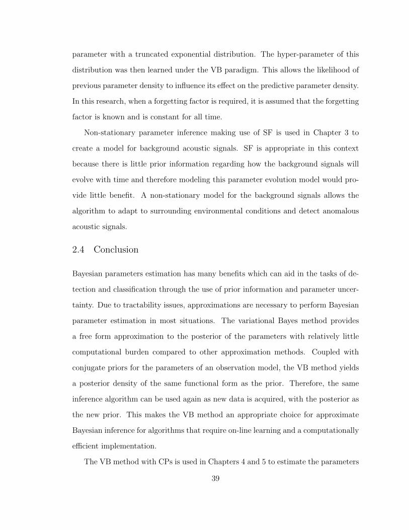
parameter with a truncated exponential distribution. The hyper-parameter of this

distribution was then learned under the VB paradigm. This allows the likelihood of

previous parameter density to influence its effect on the predictive parameter density.

In this research, when a forgetting factor is required, it is assumed that the forgetting

factor is known and is constant for all time.

Non-stationary parameter inference making use of SF is used in Chapter 3 to

create a model for background acoustic signals. SF is appropriate in this context

because there is little prior information regarding how the background signals will

evolve with time and therefore modeling this parameter evolution model would pro-

vide little benefit. A non-stationary model for the background signals allows the

algorithm to adapt to surrounding environmental conditions and detect anomalous

acoustic signals.

2.4 Conclusion

Bayesian parameters estimation has many benefits which can aid in the tasks of de-

tection and classification through the use of prior information and parameter uncer-

tainty. Due to tractability issues, approximations are necessary to perform Bayesian

parameter estimation in most situations. The variational Bayes method provides

a free form approximation to the posterior of the parameters with relatively little

computational burden compared to other approximation methods. Coupled with

conjugate priors for the parameters of an observation model, the VB method yields

a posterior density of the same functional form as the prior. Therefore, the same

inference algorithm can be used again as new data is acquired, with the posterior as

the new prior. This makes the VB method an appropriate choice for approximate

Bayesian inference for algorithms that require on-line learning and a computationally

efficient implementation.

The VB method with CPs is used in Chapters 4 and 5 to estimate the parameters

39

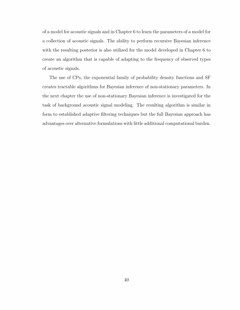
of a model for acoustic signals and in Chapter 6 to learn the parameters of a model for

a collection of acoustic signals. The ability to perform recursive Bayesian inference

with the resulting posterior is also utilized for the model developed in Chapter 6 to

create an algorithm that is capable of adapting to the frequency of observed types

of acoustic signals.

The use of CPs, the exponential family of probability density functions and SF

creates tractable algorithms for Bayesian inference of non-stationary parameters. In

the next chapter the use of non-stationary Bayesian inference is investigated for the

task of background acoustic signal modeling. The resulting algorithm is similar in

form to established adaptive filtering techniques but the full Bayesian approach has

advantages over alternative formulations with little additional computational burden.

40

3

Detection of Anomalous Acoustic Signals

The previous chapter discussed Bayesian parameter inference techniques for both

stationary and non-stationary parameters. The remainder of this work is focused on

the development of Bayesian inference for models applicable to acoustic sensing tasks.

In this chapter, the task of detecting anomalous signals from within background

sounds is considered. The approach is based on a Bayesian learning algorithm for

the non-stationary parameters of a model for the time-domain background acoustic

signals. Deviations from this model are then used to infer the arrival of anomalous

acoustic signals. The chapter begins by analyzing typical background signals and

signals that are to be detected from an acoustic surveillance perspective.

3.1 Acoustic Surveillance

As previously stated in Chapter 1, the goal of the acoustic surveillance is to detect

acoustic signals that are indicative of a security breach or some other anomalous

event on an enclosed premises. These types of sounds may include gun shots, break-

ing glass, and door slams. Detection of the sounds of interest is made difficult by the

presence of background signals with spectral properties that vary over time. Back-

41

Figure 3.1: An example impulsive sound masked by background noise. A sampleof gun fire has been artificially embedded within a sample of traffic noise. The gunfire occurs at 6.75 s. The top plot shows the time-domain representation and thebottom plot shows the STFT.

ground sounds may vary with parameters such as sensor location, time of day, and

weather conditions, and include such causes as wind, traffic, and nature sounds in

outdoor environments or ventilations system and machine noise in indoor environ-

ments. Fig. 3.1 shows data from an example situation that may be encountered by

an outdoor acoustic surveillance system. The system is located near a busy street

and thus there is traffic noise received by the system at all times. A muzzle blast

signal is received by the system at approximately 6.75 s. However, due to the ambi-

ent street noise it is nearly entirely masked in the time domain (top plot). However,

the spectral difference between the two signals make the arrival of the muzzle blast

visibly apparent in the short time Fourier transform (STFT) (bottom plot).

Other acoustic signals that may be of interest to an acoustic surveillance system

are shown in Fig. 3.2. This figure demonstrates that each of these signals can be

characterized by an impulsive high energy period followed by a energy decay. As-

suming normal background conditions, the arrival of these signals will thus result

in a dramatic spectral changes in the received acoustic signal. Therefore, even in

42

Figure 3.2: Example time-domain representation of sounds of interest in acousticsurveillance: gun fire (top), glass breaking (middle), and a door slam (bottom).

the presence high energy background signals, spectral differences will offer a means

to detect the arrival of a low energy but anomalous signal. However, due to the

complex nature of the sounds of interest, a sophisticated model is required to distin-

guish between differnt anamolous acoustic signals (see Chapter 6) and it would be

intractible to apply this model to each new time sample as it arrives. Instead, the

approach taken in this chapter is to discriminate them from the background signals

by detecting deviations from a background signal model. Therefore, a signal model

capable of accurately modeling the ambient background signals is required.

Given that the sounds of interest to an acoustic surveillance system have differ-

ent spectral characteristics than typical background sounds, it is logical to desire a

background signal model which captures the spectral characteristics of typical back-

ground sounds. Based on the physical nature of the sounds of interest, it may then

follow that this model should operate in the frequency domain despite the fact that

data received from the microphone is a time series. However, transforming this data

into the frequency domain would require ad hoc decisions regarding the transform,

43

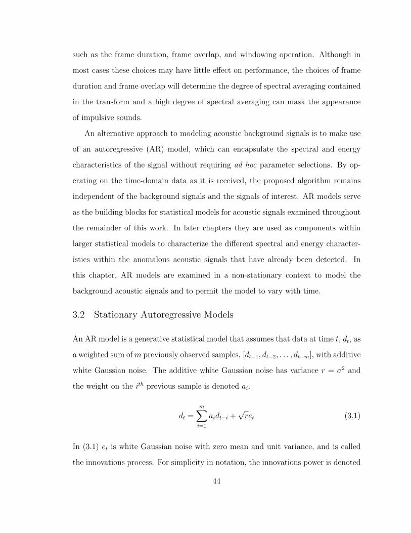
such as the frame duration, frame overlap, and windowing operation. Although in

most cases these choices may have little effect on performance, the choices of frame

duration and frame overlap will determine the degree of spectral averaging contained

in the transform and a high degree of spectral averaging can mask the appearance

of impulsive sounds.

An alternative approach to modeling acoustic background signals is to make use

of an autoregressive (AR) model, which can encapsulate the spectral and energy

characteristics of the signal without requiring ad hoc parameter selections. By op-

erating on the time-domain data as it is received, the proposed algorithm remains

independent of the background signals and the signals of interest. AR models serve

as the building blocks for statistical models for acoustic signals examined throughout

the remainder of this work. In later chapters they are used as components within

larger statistical models to characterize the different spectral and energy character-

istics within the anomalous acoustic signals that have already been detected. In

this chapter, AR models are examined in a non-stationary context to model the

background acoustic signals and to permit the model to vary with time.

3.2 Stationary Autoregressive Models

An AR model is a generative statistical model that assumes that data at time t, dt, as

a weighted sum of m previously observed samples, [dt−1, dt−2, . . . , dt−m], with additive

white Gaussian noise. The additive white Gaussian noise has variance r = σ2 and

the weight on the ith previous sample is denoted ai.

dt =m∑i=1

aidt−i +√ret (3.1)

In (3.1) et is white Gaussian noise with zero mean and unit variance, and is called

the innovations process. For simplicity in notation, the innovations power is denoted

44

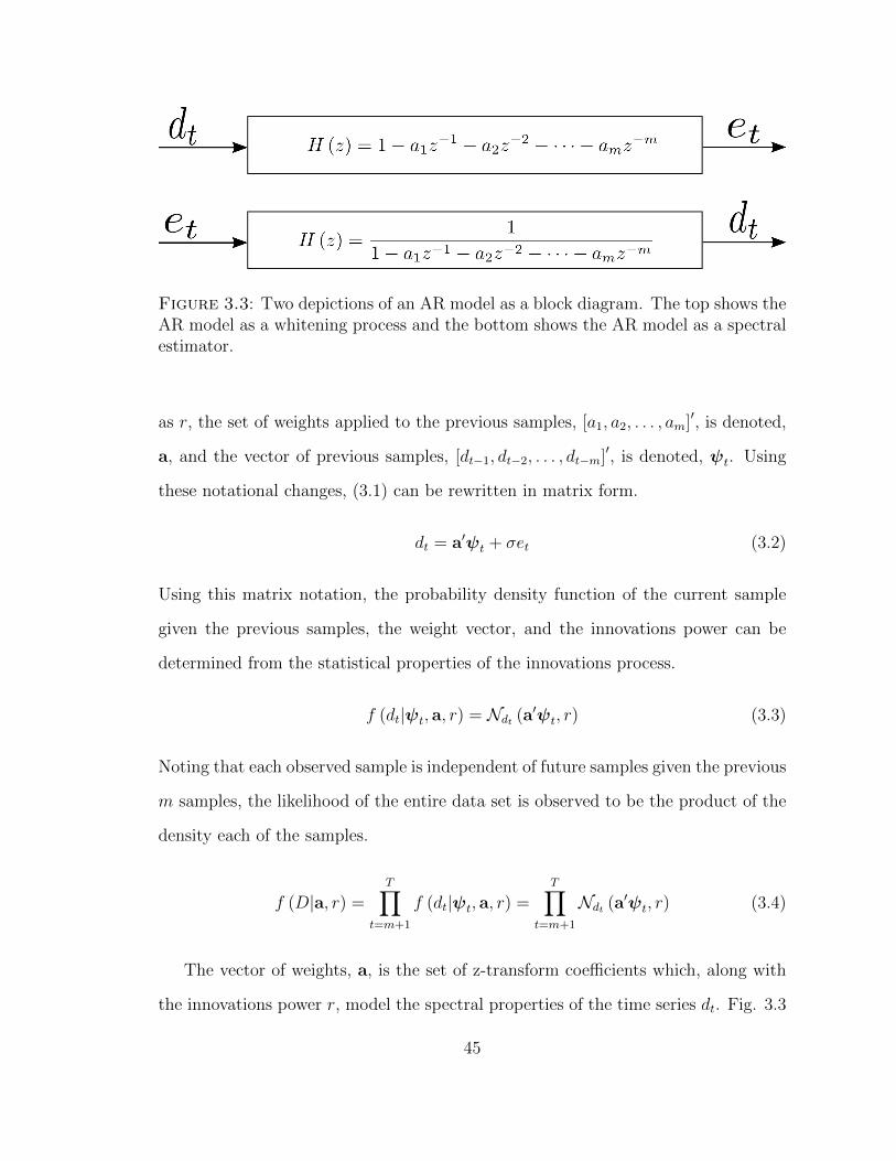
Figure 3.3: Two depictions of an AR model as a block diagram. The top shows theAR model as a whitening process and the bottom shows the AR model as a spectralestimator.

as r, the set of weights applied to the previous samples, [a1, a2, . . . , am]′, is denoted,

a, and the vector of previous samples, [dt−1, dt−2, . . . , dt−m]′, is denoted, ψt. Using

these notational changes, (3.1) can be rewritten in matrix form.

dt = a′ψt + σet (3.2)

Using this matrix notation, the probability density function of the current sample

given the previous samples, the weight vector, and the innovations power can be

determined from the statistical properties of the innovations process.

f (dt|ψt, a, r) = Ndt (a′ψt, r) (3.3)

Noting that each observed sample is independent of future samples given the previous

m samples, the likelihood of the entire data set is observed to be the product of the

density each of the samples.

f (D|a, r) =T∏

t=m+1

f (dt|ψt, a, r) =T∏

t=m+1

Ndt (a′ψt, r) (3.4)

The vector of weights, a, is the set of z-transform coefficients which, along with

the innovations power r, model the spectral properties of the time series dt. Fig. 3.3

45

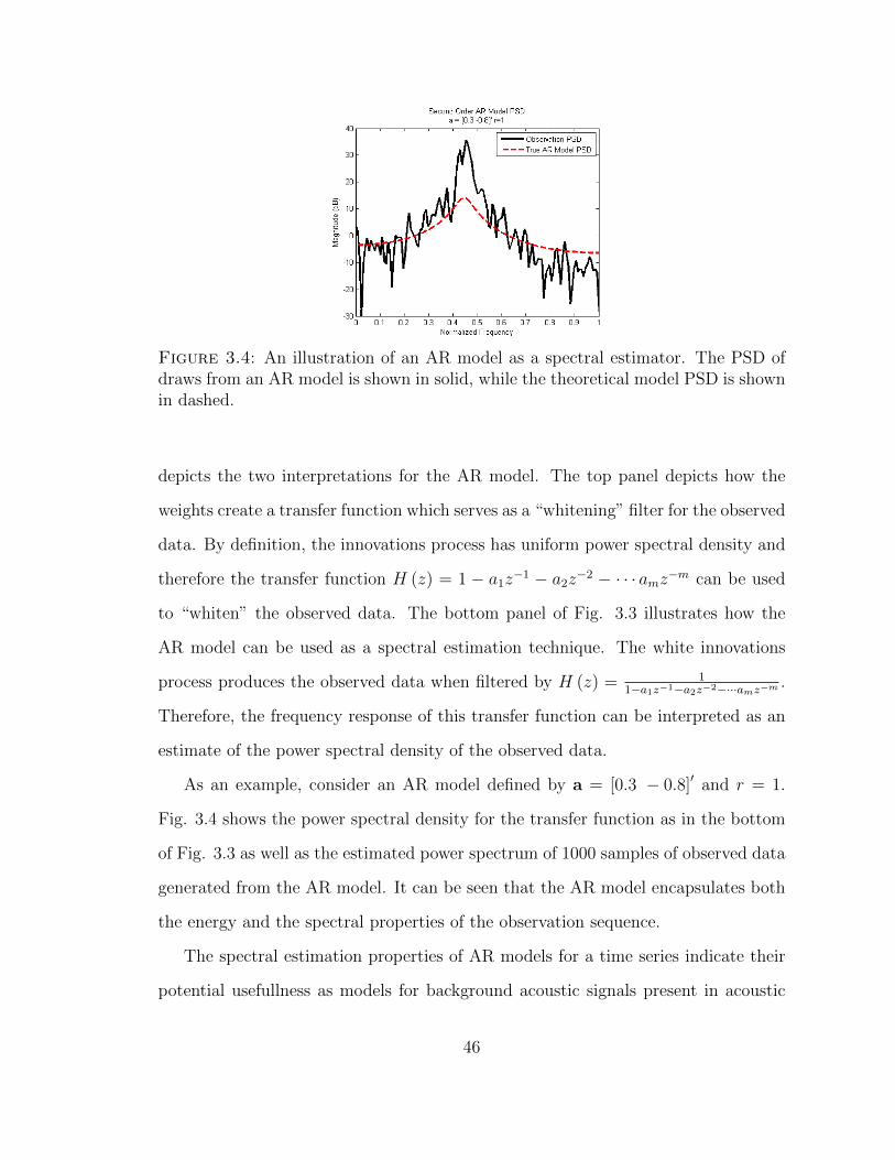
Figure 3.4: An illustration of an AR model as a spectral estimator. The PSD ofdraws from an AR model is shown in solid, while the theoretical model PSD is shownin dashed.

depicts the two interpretations for the AR model. The top panel depicts how the

weights create a transfer function which serves as a “whitening” filter for the observed

data. By definition, the innovations process has uniform power spectral density and

therefore the transfer function H (z) = 1 − a1z−1 − a2z

−2 − · · · amz−m can be used

to “whiten” the observed data. The bottom panel of Fig. 3.3 illustrates how the

AR model can be used as a spectral estimation technique. The white innovations

process produces the observed data when filtered by H (z) = 11−a1z−1−a2z−2−···amz−m .

Therefore, the frequency response of this transfer function can be interpreted as an

estimate of the power spectral density of the observed data.

As an example, consider an AR model defined by a = [0.3 − 0.8]′ and r = 1.

Fig. 3.4 shows the power spectral density for the transfer function as in the bottom

of Fig. 3.3 as well as the estimated power spectrum of 1000 samples of observed data

generated from the AR model. It can be seen that the AR model encapsulates both

the energy and the spectral properties of the observation sequence.

The spectral estimation properties of AR models for a time series indicate their

potential usefullness as models for background acoustic signals present in acoustic

46

surveillance tasks. To test the efficacy of AR models for modeling background acous-

tic signals, it is necessary to analyze the methods for training AR models. Specifically,

both ML and Bayesian solutions will be examined.

3.2.1 Maximum Likelihood Estimation

Maximum likelihood estimation of the parameters which define an AR model is a well

established technique [53]. The solution for AR model weights is often interpreted

as minimizing the squared error between the current sample, dt, and the predicted

sample, a′ψt, with additive white Gaussian noise. The same solution can be derived

by maximizing (3.4) with respect to each of the parameters, a and r.

log f (D|a, r) = log (2πr)(−T−m2

) − 1

2r

T∑t=m+1

(dt − a′ψt)2

(3.5)

= log (2πr)(−T−m2

) +1

2r

T∑t=m+1

d2t − 2a′ψtdt + a′ψtψ

′ta (3.6)

To find the ML solution for the AR weights this equation is differentiated with respect

to a.

∂

∂alog f (D|a, r) =

1

2r

T∑t=m+1

−2ψtdt + 2a′ψtψ′t (3.7)

Setting this quantity equal to zero yields

T∑t=m+1

ψtdt =T∑

t=m+1

a′ψtψ′t. (3.8)

If both sides of this equation a normalized by the number of samples, T −m, it can

be seen that the left hand side is the first m terms of the auto-correlation sequence

of the observed data, rd = [rd (1) , rd (2) , . . . , r (m)]′ and the right hand side is the

47

vector of AR weights multiplied by the correlation matrix for the observed data,

denoted as R.

Rd =

rd (0) rd (1) · · · rd (m− 1)rd (1) rd (0) · · · rd (m− 2)

......

. . ....

rd (m− 1) rd (m− 2) · · · rd (0)

. (3.9)

rd = Rda (3.10)

This set of equations is known as the Yule-Walker equations. They can be solved to

yield the ML estimate of the AR weights through left multiplication of the inverse

correlation matrix.

aML = R−1d rd. (3.11)

Therefore, ML estimation of the of the AR weights can be found through linear al-

gebra applied to the auto-correlation and cross-correlation sequences of the observed

data.

ML estimation of the innovations power can be found by differentiating (3.5) with

respect to σ =√r.

∂

∂σlog f (D|a, r) =− T −m

σ+

1

σ3

T∑t=m+1

(dt − a′ψt)2

(3.12)

Setting this quantity equal to zero and multiplying by σ yields the following.

− (T −m) +1

σ2

T∑t=m+1

(dt − a′ψt)2

= 0 (3.13)

Solving for r = σ2 and substituting a with aML the ML solution for the innovations

power is

rML =1

T −m

T∑t=m+1

(dt − a′MLψt)2. (3.14)

48

Therefore, the ML estimate of the innovations power is dependent on the estimate

of the AR model weights. Once the ML estimate for the AR model weights has been

found, the ML estimate of the innovations power is found by determining the sample

variance of estimated innovations process.

3.2.2 Bayesian Estimation

As discussed in Chapter 2, Bayesian parameter estimation for generative statistical

models provides a posterior density for the parameters that govern the model as

opposed to point estimates for the parameters provided by ML learning. The variance

of the posterior density can then be thought of as reflecting the “confidence” in the

estimated values. As will be seen, Bayesian parameter estimation of AR models leads

to a posterior density which has a mean equal to the ML solution for the parameters.

The Bayesian formulation presented here thus serves as a generalization of the ML

approach discussed above.

Bayesian parameter estimation for AR models has previously been examined

[54, 52, 55, 56]. There are two variations within these approaches, but both begin

by defining a Normal-Inverse-Wishart prior for the joint density of the AR weights

and the innovations power. The Normal-inverse-Wishart density (see Appendix A) is

defined such that the AR weights are distributed as a multi-variate Normal given the

innovations power and the innovations power is distributed as an inverse-Wishart.

The inverse-Wishart is a probability density over covariances which enforces the pos-

itive definite property as discussed briefly in Chapter 2. The difference between the

two implementations ([54] and [56]) is the parameterization of the Normal-Inverse-

Wishart density. The parameterization used in this work is that of [52, 55, 56] where

the Normal-inverse-Wishart density is parameterized by an (m+ 1) × (m+ 1) ma-

trix V0 and scalar ν0. This notation for the Normal-inverse-Wishart is known as

49

extended regressor form.

f (a, r|V, ν) = N iWa,r (V, ν) (3.15)

=r−

ν2

Z (V, ν)e−

12r

[−1,a]V[−1,a]′ (3.16)

In this definition Z (V, ν) is a normalizing constant. Its definition is given in Ap-

pendix A. The matrix V can be decomposed into several sub-matrices,

V =

[V11 V′a1

Va1 Vaa

], (3.17)

where the sub-matrices have the following dimensions.

V11 ∈ R

Va1 ∈ Rm×1

Vaa ∈ Rm×m

(3.18)

Using these sub-matrices the conditional density of the AR model weights given the

innovations power and the marginal density of the innovations power are

f (a|r,V, ν) = Na

(V−1aa Va1, rV

−1aa

), (3.19)

f (r|V, ν) = iWr

(ν

2,λ

2

), (3.20)

where

λ = V11 −V′a1V−1aa Va1 (3.21)

and iWr (a, b) represents the inverse-Wishart density with degrees of freedom shape

parameter a and inverse scale parameter b (see Appendix A).

The Normal-inverse-Wishart density expressed in this form is determined more

succinctly by just the two quantities, ν and V, than the alternate parameterization

presented in [54] where the density is defined by parameters of the marginal densities.

Also, using the Normal-inverse-Wishart expressed in extended regressor form leads to

50

more simplified notation when learning the posterior density as only two parameters

need to be updated instead of four.

The Normal-inverse-Wishart density is the CP for the AR model expressed in

(3.3) and as such it is expected that the posterior density, f (a, r|D), will have the

same form as the prior with updated hyperparameters V and ν.

f (a, r|D) = N iWa,r (V, ν) (3.22)

The task of Bayesian parameter estimation of the AR model is to determine the

update equations for V and ν in terms of the prior hyperparameters, V0, ν0, and the

dataset D. The update equations are determined through the following derivation.

f (a, r|D) ∝ f (D|a, r) f (a, r|V0, ν0) (3.23)

=T∏

t=m+1

f (dt|a, r) f (a, r|V0, ν0) (3.24)

=T∏

t=m+1

Ndt (a′ψt, r)N iWa,r (V0, ν0) (3.25)

=T∏

t=m+1

(2πr)−12 e−

12r

(dt−a′ψt)2 r−

12ν0

Z (V0, ν0)e−

12r

[−1,a′]V0[−1,a′]′ (3.26)

=(2π)−

12

(T−m)

Z (V0, ν0)r−

12

(ν0+T−m)·

e

− 12r

T∑

t=m+1

((dt − a′ψt)

2)

+([−1, a′] V0 [−1, a′]

′)(3.27)

=(2π)−

12

(T−m)

Z (V0, ν0)r−

12

(ν0+T−m)e

− 12r

[−1,a′]

T∑

t=m+1

(φtφ′t) + V0

[−1,a′]′

(3.28)

In (3.28) the quantity φt = [dt, ψ′t]′ has been introduced. As anticipated, the end

51

result has the form of the Normal-inverse-Wishart with updated hyperparameters.

f (a, r|D) = N iWa,r

(V0 +

T∑t=m+1

φtφ′t, ν0 + T −m

)(3.29)

Bayesian parameter estimation for the AR model with a prior parameterized by V0

and ν0 is as simple as updating the hyperparameters.

V = V0 +T∑

t=m+1

φtφ′t (3.30)

ν = ν0 + T −m (3.31)

If the influence of the prior hyperparameters, V0 and ν0 is omitted by assum-

ing that they are equal to zero, insight about the posterior hyperparameters can

be gained. From inspection of the partition of the hyper-parameter, V, and the

update equations above, it can be seen that the sub-matrix Vaa corresponds to the

unnormalized estimate of the correlation matrix, (T −m)Rd. Furthermore, it can

be seen that the normalizing constant is equal to ν. Thus ν is a measure of the

number of samples from which our posterior density is determined. Similarly, it can

be seen that the sub-vector V1a is equal to the first m terms of the unnormalized

auto-correlation sequence of the observed data (T −m) rd. From these observations

it can be seen that the posterior marginal mean for the AR model weights is equal

to the ML solution.

a = V−1aa V1a = (T −m) V−1

aa

1

T −mV1a = R−1

d rd (3.32)

The mean of the marginal distribution of the innovations power is given by 1T−2

λ

(See Appendix A). The derived parameter λ can be decomposed using the above

definitions for Va1 and Vaa along with the observation that V11 is the unnormalized

auto-correlation evaluated at zero, (T −m) rd (0).

λ = V11 −V′a1V−1aa Va1 = (T −m) rd (0)−V′a1a = (T −m) [rd (0)− r′da] (3.33)

52

Therefore, it can be seen that the mean of the marginal posterior density for the

innovations power is equal to the ML solution of the innovations power (see [53]).

As in the above analysis, it is often desirable to have the prior have very little

influence on the outcome of the Bayesian parameter estimation. Priors of this form

are referred to as diffuse priors. As discussed above, the parameter ν indicates

the number of samples from which our current posterior estimate is derived. A

diffuse prior for the AR model is therefore given by setting ν0 to be a small number.

Throughout this research the Normal-inverse-Wishart parameters of the prior density

for an AR model of order m are set such that the prior density of AR weights has zero

mean and diagonal covariance matrix σ2aIm, with a large σ2

a, and the prior density

for the innovations power has mean of 1 and an arbitrarily large variance σ2r . Using

(3.17 - 3.20), the (m+ 1)× (m+ 1) matrix V0 and the scalar ν0 can be shown to be

equal to

V0 =

σ−2r 0 · · · 00 σ−2

a 0 0... 0

. . . 00 0 · · · σ−2

a

(3.34)

ν0 = σ−2r . (3.35)

The values of σ2a and σ2

r are each set to 1000 throughout this work.

Because the Normal-inverse-Wishart is the CP to the AR model, analytic calcu-

lation of the evidence and thus the predictive density is possible. Given a posterior

density for the AR model trained from a dataset, f (a, r|D), the analytic solution

to the marginal density for a data point can be found to be Student’s t distribution

[30].

f (dT+1|ψT+1, D) =

∫f (dT+1|a, r) f (a, r|D) dadr = StdT+1

(V−1aa Va1, λ, ν

)(3.36)

53

This density can be used to perform additional inference, for example the likelihood

ratio test.

3.3 Non-Stationary Autoregressive Models

3.3.1 Maximum Likelihood Estimation

Maximum likelihood estimation of non-stationary AR models is also well established

technique in the field of adaptive filters. The solution gives rise to the LMS algorithm

[53] which is presented here for completeness. The ML estimate of the AR weights,

at time t is denoted as at. This quantity must be estimated from the current data, dt,

the m previous samples, ψt, and the previous AR weights, at−1. This is accomplished

through gradient ascent of the log-likelihood of the parameters. The log-likelihood

of at and rt is given by

log f (dt|a, r) =− 1

2log (2πrt)−

1

2rt(dt − a′tψt)

2(3.37)

=− 1

2log (2πrt)−

1

2rt

(d2t − 2a′tψtdt + a′tψtψ

′tat)

(3.38)

This is similar to the log of (3.3) but the parameters a and r have been replaced by

their values at time t, at and rt. It is desired to perform gradient ascent to find the

estimate of the AR weights at time t+ 1.

at+1 = at + µ∂

∂alog f (dt|at, rt) (3.39)

In (3.39), µ is the learning rate and must be set experimentally. The gradient of the

likelihood with respect to the AR weights can be found to be

∂

∂alog f (dt|at, rt) =

1

rtψt [dt −ψ′tat] . (3.40)

It can be seen that the leading fraction is not a function of the data and thus

can be combined into the learning rate, µa. Using this expression the maximum

54

likelihood estimation of a non-stationary AR model consists of updating the AR

weights according to

at+1 = at + µψt (dt −ψ′tat) (3.41)

This solution is identical to the solution that is reached if gradient descent is

used to minimize the mean squared error of the predicted signal. Approaching the

problem from this point of view does not lend itself to estimation of the innovations

power. Although an estimate of the innovations power can be determined at each

time by performing gradient ascent over the log likelihood, this is not typically done.

The details associated with the use of the LMS algorithm for acoustic surveillance

are discussed in Section 3.4.1

3.3.2 Bayesian Estimation

ML estimation for non-stationary AR models lead to the LMS algorithm. The LMS

algorithm determines an instantaneous estimate of the AR weights but typically, not

an instantaneous estimate of the innovations power. Bayesian parameter estimation

of non-stationary AR models can provide an instantaneous estimate of both the

AR weights as well as the innovations power with little additional computational

overhead.

Bayesian parameter estimation of the AR model under non-stationary conditions

can be performed using the Bayesian AR model shown in Section 3.2.2 along with the

stabilized forgetting technique introduced in Section 2.3.1. Bayesian non-stationary

AR (BNSAR) models have been previously considered in [55, 56, 52, 57]. Typi-

cally, there is little prior information regarding the manner in which the AR model

changes through time and therefore SF is an appropriate choice for non-stationary

AR modeling.

Recall from Section 2.3.1 that the SF paradigm estimates the density of param-

eters at time t given the data scene up to and including time t− 1 as the geometric

55

mean of the posterior parameter density estimate at time t− 1 and a reference den-

sity. The two quantities in the geometric mean are weighted by γ, known as the

forgetting factor.

f (θt|Dt−1) ∝ fθt−1 (θt|Dt−1)γ f0 (θt|Dt−1)(1−γ) . (3.42)

It was also stated in Section 2.3.1 that if both the posterior parameter density and

the reference density are the members of the same exponential familty distribution,

then the geometric mean will also be a member of the same exponential family

distribution.

As discussed previously, the posterior density for the Bayesian AR model is the

Normal-inverse-Wishart, a member of the exponential family. Therefore, by selecting

the reference density to also be a Normal-inverse-Wishart the SF predictive param-

eter density will be of the same form. Assume that the reference density is defined

by the hyperparameters V0 and ν0, and parameter density at time t − 1 is defined

by hyperparameters Vt−1 and νt−1. In this case the SF predictive AR density is

determined as follows.

f (at, rt|Dt−1) ∝ fat−1,rt−1 (at, rt|Dt−1)γ f0 (at, rt|Dt−1)(1−γ) (3.43)

= N iWat,rt (γVt−1 + (1− γ) V0, λtνt−1 + (1− γ) ν0) (3.44)

The geometric mean of the two densities results in the same functional form where

the hyperparameters are a weighted sum of previous two densities’ hyperparame-

ters. From this predictive density the posterior of the parameters given dt can be

determined using the analysis given in (3.23 - 3.28). Therefore, the posterior den-

sity of the parameters is a Normal-inverse-Wishart density defined by the following

hyperparameters.

Vt = γVt−1 +ψtψ′ + (1− γ) V0 (3.45)

νt = γνt−1 + 1 + (1− γ) ν0 (3.46)

56

In most applications the reference distribution should be chosen such that it has

little influence on the AR model. In this research the reference density hyperparam-

eters are chosen to be the same as the diffuse AR parameter density described by

(3.34 - 3.35). With these hyperparameters the reference density serves to limit the

confidence of previous data and enforce a more diffuse posterior density.

3.3.3 Comparison of BNSAR Models and LMS

The use of non-stationary AR models in this research is motivated by the desire

to model the non-stationary background signals encountered in the acoustic surveil-

lance task of gunshot detection. To this point, both non-stationary ML AR models

and BNSAR models have been discussed, however, no quantitative comparison has

been made as to their theoretical performance. Despite the introduction of the non-

stationary Bayesian AR model in [52] and [57], no formal comparison of the Bayesian

solution to the ML solution has been offered in the literature. A theoretical under-

standing of both learning methods is required to gain insight about their efficacy to

the gunshot detection problem.

This section compares the two learning methods for non-stationary AR models by

comparing results obtained from two synthetic datasets and a sample of data similar

to the data expected to be observed in gunshot detection task. The first simulated

data scenario examines the performance of the two non-stationary AR models when

the observed data has an instantaneous change in the AR model. The second sim-

ulated scenario simulates a slowly changing AR model via a linear frequency chirp.

These two synthetic datasets provide insight into the theoretical performance of the

learning algorithms to respond to both rapidly and slowly varying spectral infor-

mation. The real data comparison is conducted using an example of the ambient

background sounds expected to be observed in the gunshot detection task.

Comparison of Bayesian and ML approaches to non-stationary AR modeling is

57

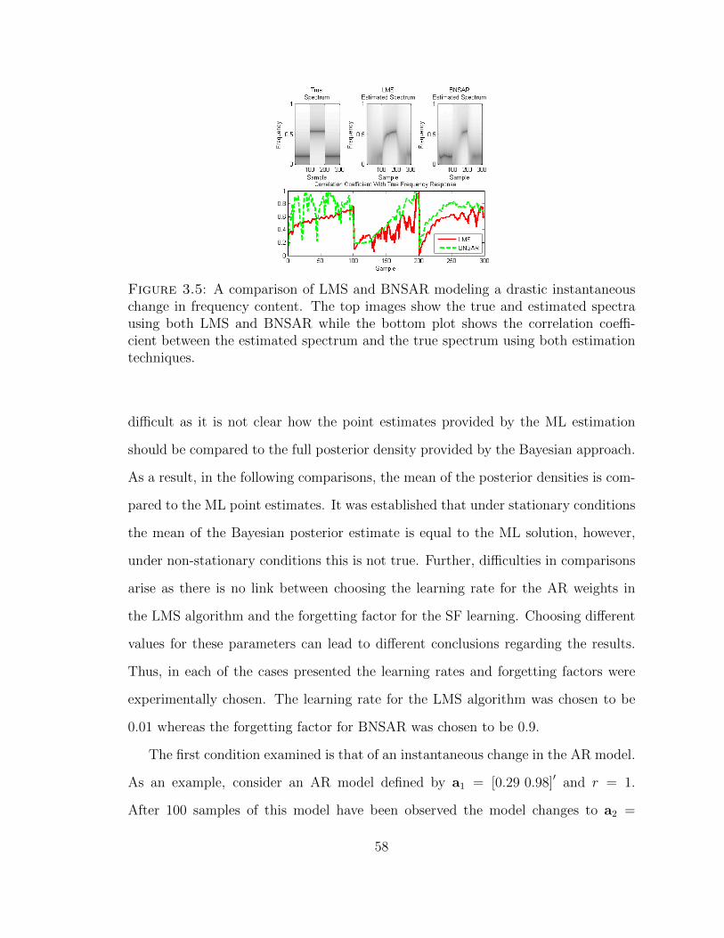
Figure 3.5: A comparison of LMS and BNSAR modeling a drastic instantaneouschange in frequency content. The top images show the true and estimated spectrausing both LMS and BNSAR while the bottom plot shows the correlation coeffi-cient between the estimated spectrum and the true spectrum using both estimationtechniques.

difficult as it is not clear how the point estimates provided by the ML estimation

should be compared to the full posterior density provided by the Bayesian approach.

As a result, in the following comparisons, the mean of the posterior densities is com-

pared to the ML point estimates. It was established that under stationary conditions

the mean of the Bayesian posterior estimate is equal to the ML solution, however,

under non-stationary conditions this is not true. Further, difficulties in comparisons

arise as there is no link between choosing the learning rate for the AR weights in

the LMS algorithm and the forgetting factor for the SF learning. Choosing different

values for these parameters can lead to different conclusions regarding the results.

Thus, in each of the cases presented the learning rates and forgetting factors were

experimentally chosen. The learning rate for the LMS algorithm was chosen to be

0.01 whereas the forgetting factor for BNSAR was chosen to be 0.9.

The first condition examined is that of an instantaneous change in the AR model.

As an example, consider an AR model defined by a1 = [0.29 0.98]′ and r = 1.

After 100 samples of this model have been observed the model changes to a2 =

58

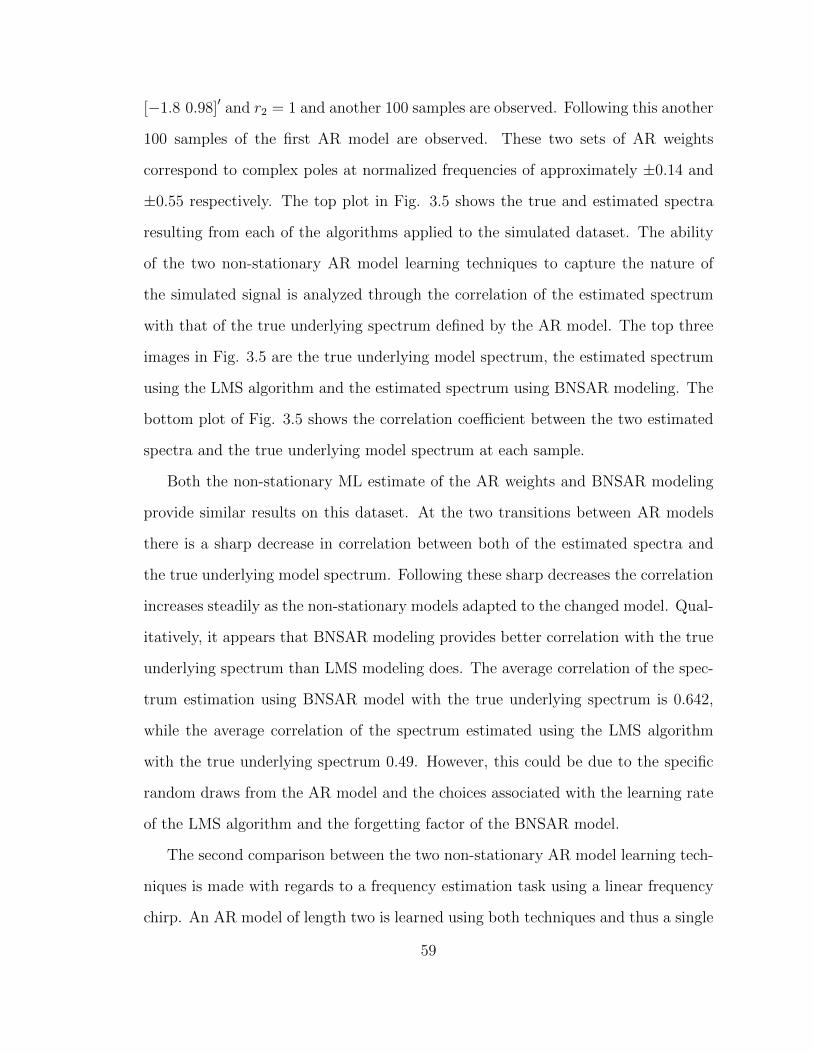
[−1.8 0.98]′ and r2 = 1 and another 100 samples are observed. Following this another

100 samples of the first AR model are observed. These two sets of AR weights

correspond to complex poles at normalized frequencies of approximately ±0.14 and

±0.55 respectively. The top plot in Fig. 3.5 shows the true and estimated spectra

resulting from each of the algorithms applied to the simulated dataset. The ability

of the two non-stationary AR model learning techniques to capture the nature of

the simulated signal is analyzed through the correlation of the estimated spectrum

with that of the true underlying spectrum defined by the AR model. The top three

images in Fig. 3.5 are the true underlying model spectrum, the estimated spectrum

using the LMS algorithm and the estimated spectrum using BNSAR modeling. The

bottom plot of Fig. 3.5 shows the correlation coefficient between the two estimated

spectra and the true underlying model spectrum at each sample.

Both the non-stationary ML estimate of the AR weights and BNSAR modeling

provide similar results on this dataset. At the two transitions between AR models

there is a sharp decrease in correlation between both of the estimated spectra and

the true underlying model spectrum. Following these sharp decreases the correlation

increases steadily as the non-stationary models adapted to the changed model. Qual-

itatively, it appears that BNSAR modeling provides better correlation with the true

underlying spectrum than LMS modeling does. The average correlation of the spec-

trum estimation using BNSAR model with the true underlying spectrum is 0.642,

while the average correlation of the spectrum estimated using the LMS algorithm

with the true underlying spectrum 0.49. However, this could be due to the specific

random draws from the AR model and the choices associated with the learning rate

of the LMS algorithm and the forgetting factor of the BNSAR model.

The second comparison between the two non-stationary AR model learning tech-

niques is made with regards to a frequency estimation task using a linear frequency

chirp. An AR model of length two is learned using both techniques and thus a single

59

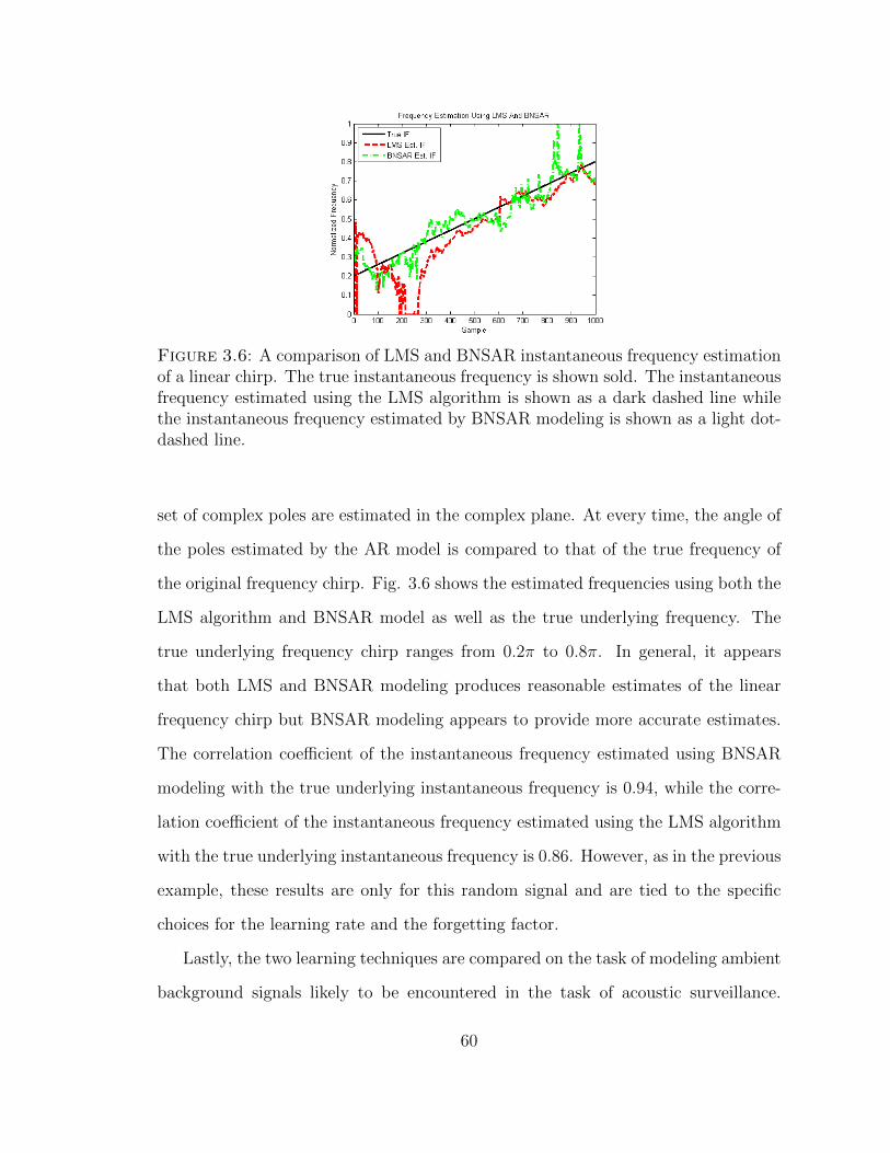
Figure 3.6: A comparison of LMS and BNSAR instantaneous frequency estimationof a linear chirp. The true instantaneous frequency is shown sold. The instantaneousfrequency estimated using the LMS algorithm is shown as a dark dashed line whilethe instantaneous frequency estimated by BNSAR modeling is shown as a light dot-dashed line.

set of complex poles are estimated in the complex plane. At every time, the angle of

the poles estimated by the AR model is compared to that of the true frequency of

the original frequency chirp. Fig. 3.6 shows the estimated frequencies using both the

LMS algorithm and BNSAR model as well as the true underlying frequency. The

true underlying frequency chirp ranges from 0.2π to 0.8π. In general, it appears

that both LMS and BNSAR modeling produces reasonable estimates of the linear

frequency chirp but BNSAR modeling appears to provide more accurate estimates.

The correlation coefficient of the instantaneous frequency estimated using BNSAR

modeling with the true underlying instantaneous frequency is 0.94, while the corre-

lation coefficient of the instantaneous frequency estimated using the LMS algorithm

with the true underlying instantaneous frequency is 0.86. However, as in the previous

example, these results are only for this random signal and are tied to the specific

choices for the learning rate and the forgetting factor.

Lastly, the two learning techniques are compared on the task of modeling ambient

background signals likely to be encountered in the task of acoustic surveillance.

60

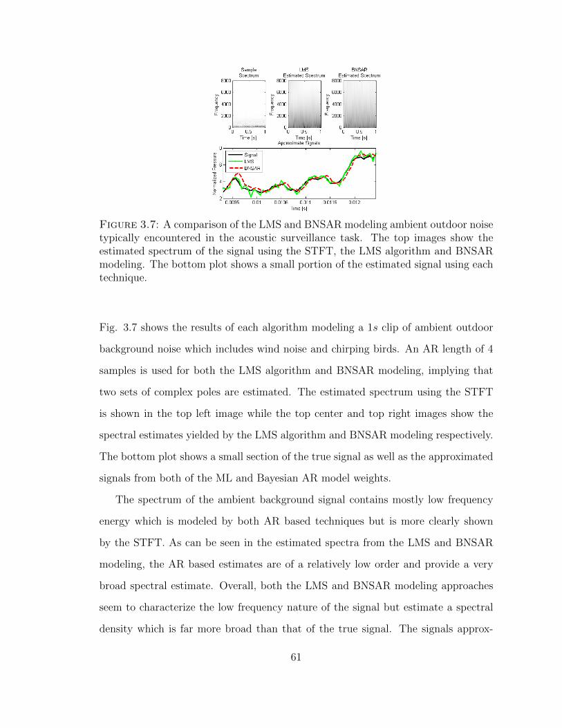
Figure 3.7: A comparison of the LMS and BNSAR modeling ambient outdoor noisetypically encountered in the acoustic surveillance task. The top images show theestimated spectrum of the signal using the STFT, the LMS algorithm and BNSARmodeling. The bottom plot shows a small portion of the estimated signal using eachtechnique.

Fig. 3.7 shows the results of each algorithm modeling a 1s clip of ambient outdoor

background noise which includes wind noise and chirping birds. An AR length of 4

samples is used for both the LMS algorithm and BNSAR modeling, implying that

two sets of complex poles are estimated. The estimated spectrum using the STFT

is shown in the top left image while the top center and top right images show the

spectral estimates yielded by the LMS algorithm and BNSAR modeling respectively.

The bottom plot shows a small section of the true signal as well as the approximated

signals from both of the ML and Bayesian AR model weights.

The spectrum of the ambient background signal contains mostly low frequency

energy which is modeled by both AR based techniques but is more clearly shown

by the STFT. As can be seen in the estimated spectra from the LMS and BNSAR

modeling, the AR based estimates are of a relatively low order and provide a very

broad spectral estimate. Overall, both the LMS and BNSAR modeling approaches

seem to characterize the low frequency nature of the signal but estimate a spectral

density which is far more broad than that of the true signal. The signals approx-

61

imated by the learned AR models follow closely to the true signal. Therefore, it

can be concluded from these small scaled experiments that both AR model based

approaches are capable of characterized relevant ambient background signals.

The results of these three qualitative experiments indicate that both LMS and

BNSAR modeling can characterize the broad spectral qualities of ambient back-

ground signals and adequately adapt to changes in these signals. Qualitatively, it

does not appear that either algorithm concretely outperforms the other in these

limited experiments. It is known, however, that BNSAR modeling provides an in-

stantaneous estimate of the innovations power after each new observation whereas

the LMS algorithm typically uses an ad hoc algorithm to estimate the innovations

power. As will be seen in the following section, an estimate of the innovations power

can be very useful for the acoustic surveillance task.

3.4 Application to Acoustic Surveillance

As was shown in the previous section both ML and Bayesian techniques for learning

non-stationary AR models are able to adequately model the ambient background sig-

nals present in acoustic surveillance settings. In this section, the two non-stationary

AR model based approaches are compared on the task of acoustic surveillance. First,

the details associated with implementing each algorithm as a gunshot detector are

discussed. Following this an illustration of the algorithms applied to the acoustic

surveillance example given in Fig. 3.1 is presented followed by a comparison of the

algorithms applied to a synthetic yet realistic dataset.

3.4.1 LMS Based Detection

The algorithm presented in this research, based on the LMS algorithm, for the task

of acoustic surveillance is based upon analysis of the error of the predicted signal.

When the LMS algorithm is accurately modeling the background ambient signals the

62

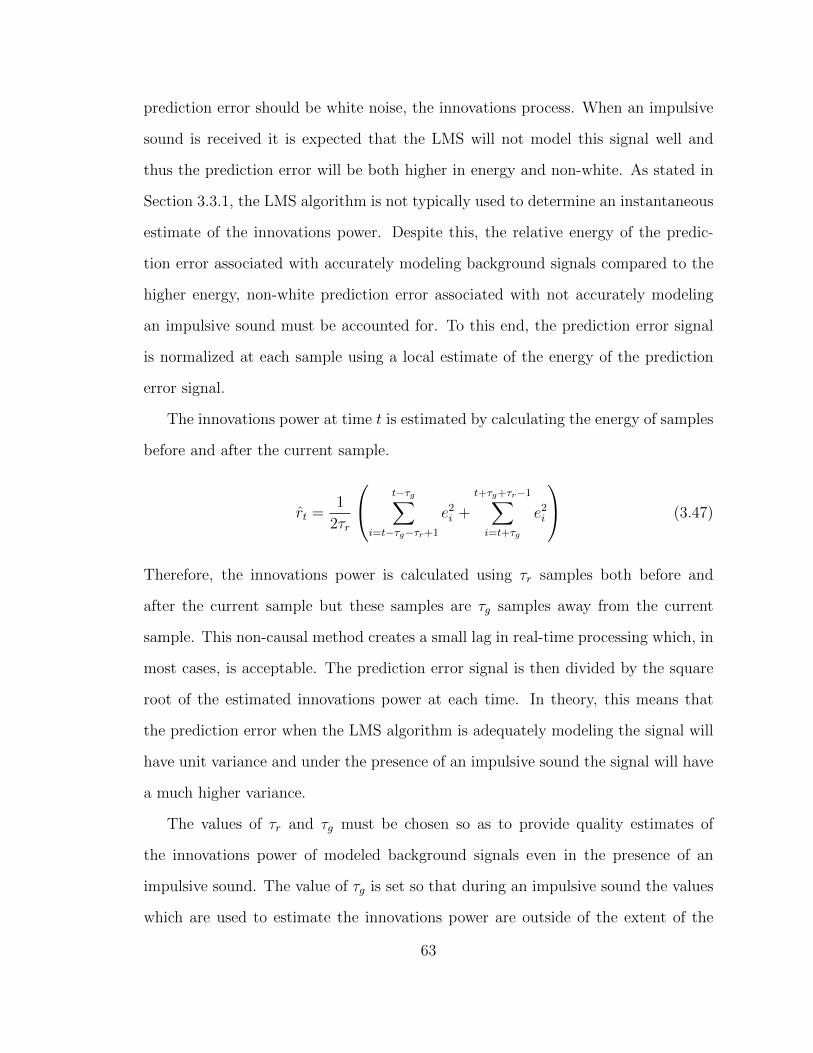
prediction error should be white noise, the innovations process. When an impulsive

sound is received it is expected that the LMS will not model this signal well and

thus the prediction error will be both higher in energy and non-white. As stated in

Section 3.3.1, the LMS algorithm is not typically used to determine an instantaneous

estimate of the innovations power. Despite this, the relative energy of the predic-

tion error associated with accurately modeling background signals compared to the

higher energy, non-white prediction error associated with not accurately modeling

an impulsive sound must be accounted for. To this end, the prediction error signal

is normalized at each sample using a local estimate of the energy of the prediction

error signal.

The innovations power at time t is estimated by calculating the energy of samples

before and after the current sample.

rt =1

2τr

t−τg∑i=t−τg−τr+1

e2i +

t+τg+τr−1∑i=t+τg

e2i

(3.47)

Therefore, the innovations power is calculated using τr samples both before and

after the current sample but these samples are τg samples away from the current

sample. This non-causal method creates a small lag in real-time processing which, in

most cases, is acceptable. The prediction error signal is then divided by the square

root of the estimated innovations power at each time. In theory, this means that

the prediction error when the LMS algorithm is adequately modeling the signal will

have unit variance and under the presence of an impulsive sound the signal will have

a much higher variance.

The values of τr and τg must be chosen so as to provide quality estimates of

the innovations power of modeled background signals even in the presence of an

impulsive sound. The value of τg is set so that during an impulsive sound the values

which are used to estimate the innovations power are outside of the extent of the

63

impulsive sound. Because impulsive sounds have a short duration, a value of τg

can be experimentally determined, which balances the quality of the local estimate

and the effect of an impulsive sound on this local estimate. The value of τr must be

determined so as to balance the quality of the estimate by having a sufficient number

of samples and still provide a local estimate of the innovations power. The value of

τg chosen in this research was based on a study of the duration of impulsive sounds

and was chosen to be 0.125s. The value of τr was also chosen experimentally and

was chosen to be 0.0625s.

Following the normalization by the local estimate of the innovations power the

normalized LMS error signal is used to determine the presence of impulsive sounds.

A fifth order AR model was chosen through experimentation as was the learning

rate, which was set to 0.01.

3.4.2 BNSAR Based Detection

Due to the full posterior of the estimate of both the innovations power and the

AR weights provided by BNSAR modeling, the normalizing techniques used in the

LMS based processing are not required for BNSAR based processing. Instead the

predictive probability density of the sample at time t + 1 is determined using the

posterior estimates of the AR weights and innovations power at time t. This proba-

bility density is used to model the likelihood of the H0 hypothesis in the likelihood

ratio test.

λ (dt) =p (dt|Dt−1, H1)

p (dt|Dt−1, H0)(3.48)

The likelihood of the H0 hypothesis is given by (3.36) but the likelihood of the H1

hypothesis has yet to be discussed. As the goal of this stage of processing is to detect

all anamalous acoustic signals no statistical model for H1 is employed. Therefore the

likelihood of the H1 hypothesis is assumed to be diffuse. To this end the data under

64

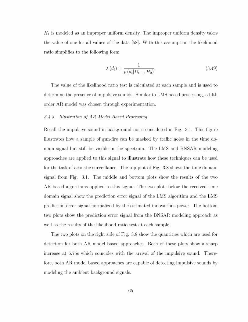
H1 is modeled as an improper uniform density. The improper uniform density takes

the value of one for all values of the data [58]. With this assumption the likelihood

ratio simplifies to the following form

λ (dt) =1

p (dt|Dt−1, H0). (3.49)

The value of the likelihood ratio test is calculated at each sample and is used to

determine the presence of impulsive sounds. Similar to LMS based processing, a fifth

order AR model was chosen through experimentation.

3.4.3 Illustration of AR Model Based Processing

Recall the impulsive sound in background noise considered in Fig. 3.1. This figure

illustrates how a sample of gun-fire can be masked by traffic noise in the time do-

main signal but still be visible in the spectrum. The LMS and BNSAR modeling

approaches are applied to this signal to illustrate how these techniques can be used

for the task of acoustic surveillance. The top plot of Fig. 3.8 shows the time domain

signal from Fig. 3.1. The middle and bottom plots show the results of the two

AR based algorithms applied to this signal. The two plots below the received time

domain signal show the prediction error signal of the LMS algorithm and the LMS

prediction error signal normalized by the estimated innovations power. The bottom

two plots show the prediction error signal from the BNSAR modeling approach as

well as the results of the likelihood ratio test at each sample.

The two plots on the right side of Fig. 3.8 show the quantities which are used for

detection for both AR model based approaches. Both of these plots show a sharp

increase at 6.75s which coincides with the arrival of the impulsive sound. There-

fore, both AR model based approaches are capable of detecting impulsive sounds by

modeling the ambient background signals.

65

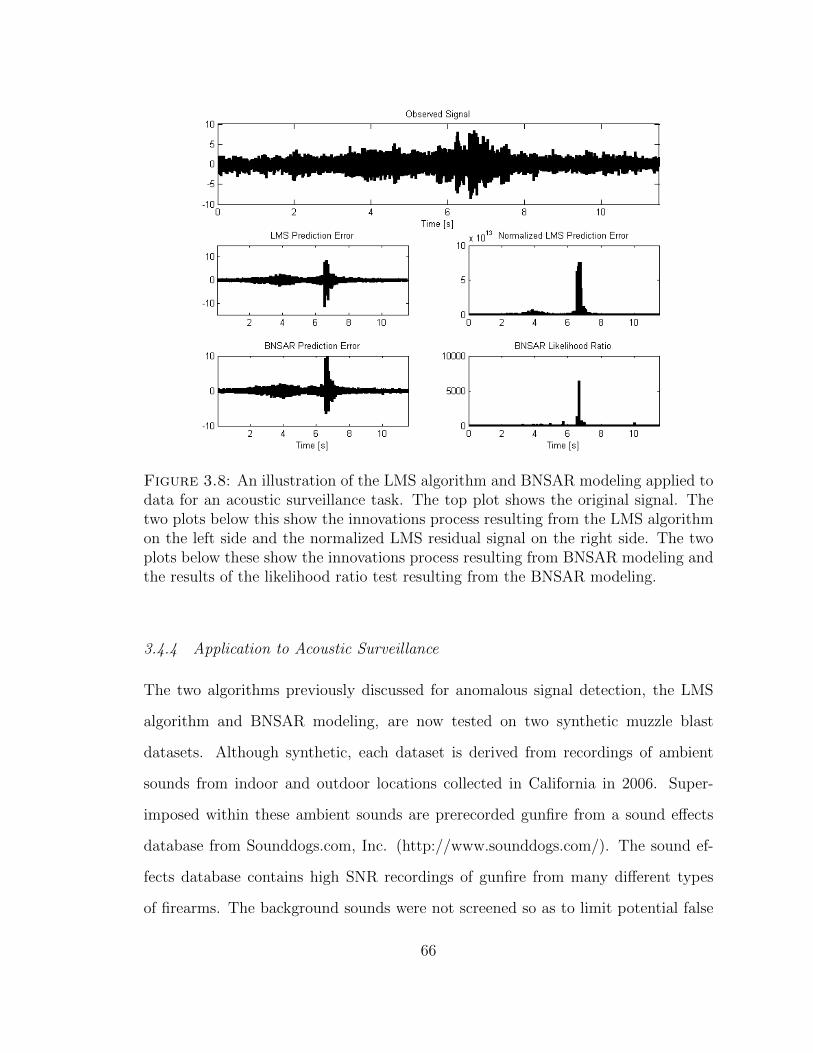
Figure 3.8: An illustration of the LMS algorithm and BNSAR modeling applied todata for an acoustic surveillance task. The top plot shows the original signal. Thetwo plots below this show the innovations process resulting from the LMS algorithmon the left side and the normalized LMS residual signal on the right side. The twoplots below these show the innovations process resulting from BNSAR modeling andthe results of the likelihood ratio test resulting from the BNSAR modeling.

3.4.4 Application to Acoustic Surveillance

The two algorithms previously discussed for anomalous signal detection, the LMS

algorithm and BNSAR modeling, are now tested on two synthetic muzzle blast

datasets. Although synthetic, each dataset is derived from recordings of ambient

sounds from indoor and outdoor locations collected in California in 2006. Super-

imposed within these ambient sounds are prerecorded gunfire from a sound effects

database from Sounddogs.com, Inc. (http://www.sounddogs.com/). The sound ef-

fects database contains high SNR recordings of gunfire from many different types

of firearms. The background sounds were not screened so as to limit potential false

66

alarms and, as a result, possible false alarms such as door slams, human speech,

animal noises, and passing traffic are contained within the data. It is believed that

although the dataset is synthetic it provides a scenario that is similar to that which

may be encountered by a gunshot detection system (GDS).

The dataset is comprised of seventy 60s recordings in indoor conditions and thirty

60s recordings in outdoor conditions. Within each of these files samples of muzzle

blasts are embedded at a specified signal to background ratio (SBR). The signal

to background ratio is defined as the ratio of the energy of the embedded signal

to the energy of the background signal in decibels calculated over the duration of

the embedded signal. No gunshots are embedded within the first 5s of each file

and following each gunshot additional gunshots are embedded delayed by a random

delay between 1s and 5s. Therefore, each file contains approximately 18 instances

of gunfire.

Because the dataset is synthetically generated, there are several parameters which

can be manipulated in a controlled experiment. The performance of the LMS al-

gorithm and BNSAR modeling can be compared individually in both indoor and

outdoor conditions at different SBR which can be enforced by adding in the gun-

fire at different intensities. When each muzzle blast is embedded, the energy of the

background signal is calculated over the duration of the muzzle blast and the energy

of the muzzle blast is adjusted to correspond to the specified SBR. Three SBR were

analyzed here, −10dB, 0dB and 10dB. The results of the muzzle blast detectioin

are then reported at each of these SBR in both indoor and outdoor conditions.

3.4.5 Results

For each set of conditions, a discrete set of alarms is determined by finding local

maximums in confidences values for a particular algorithm. Closely spaced alarms

(within 0.25s) are merged and replaced with only the alarm with the highest confi-

67

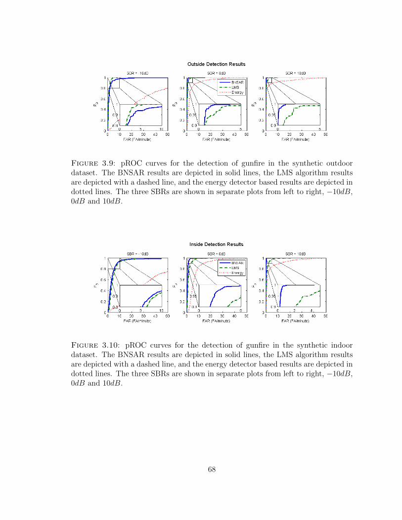
Figure 3.9: pROC curves for the detection of gunfire in the synthetic outdoordataset. The BNSAR results are depicted in solid lines, the LMS algorithm resultsare depicted with a dashed line, and the energy detector based results are depicted indotted lines. The three SBRs are shown in separate plots from left to right, −10dB,0dB and 10dB.

Figure 3.10: pROC curves for the detection of gunfire in the synthetic indoordataset. The BNSAR results are depicted in solid lines, the LMS algorithm resultsare depicted with a dashed line, and the energy detector based results are depicted indotted lines. The three SBRs are shown in separate plots from left to right, −10dB,0dB and 10dB.

68

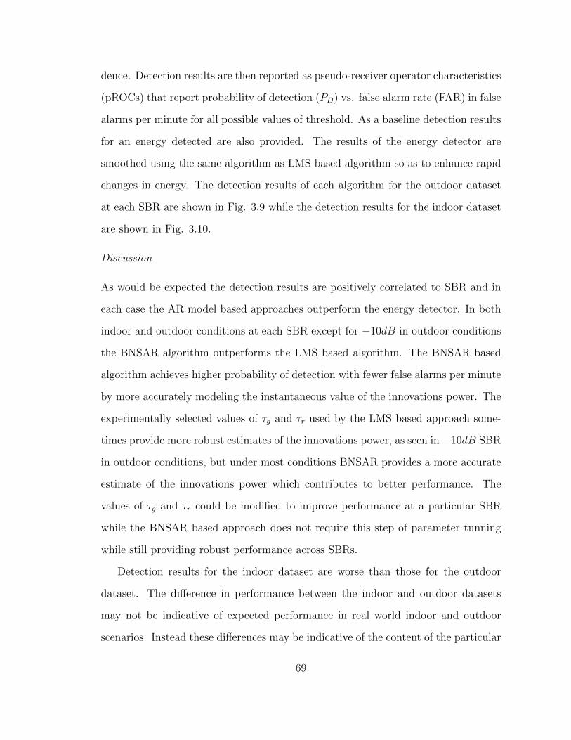
dence. Detection results are then reported as pseudo-receiver operator characteristics

(pROCs) that report probability of detection (PD) vs. false alarm rate (FAR) in false

alarms per minute for all possible values of threshold. As a baseline detection results

for an energy detected are also provided. The results of the energy detector are

smoothed using the same algorithm as LMS based algorithm so as to enhance rapid

changes in energy. The detection results of each algorithm for the outdoor dataset

at each SBR are shown in Fig. 3.9 while the detection results for the indoor dataset

are shown in Fig. 3.10.

Discussion

As would be expected the detection results are positively correlated to SBR and in

each case the AR model based approaches outperform the energy detector. In both

indoor and outdoor conditions at each SBR except for −10dB in outdoor conditions

the BNSAR algorithm outperforms the LMS based algorithm. The BNSAR based

algorithm achieves higher probability of detection with fewer false alarms per minute

by more accurately modeling the instantaneous value of the innovations power. The

experimentally selected values of τg and τr used by the LMS based approach some-

times provide more robust estimates of the innovations power, as seen in −10dB SBR

in outdoor conditions, but under most conditions BNSAR provides a more accurate

estimate of the innovations power which contributes to better performance. The

values of τg and τr could be modified to improve performance at a particular SBR

while the BNSAR based approach does not require this step of parameter tunning

while still providing robust performance across SBRs.

Detection results for the indoor dataset are worse than those for the outdoor

dataset. The difference in performance between the indoor and outdoor datasets

may not be indicative of expected performance in real world indoor and outdoor

scenarios. Instead these differences may be indicative of the content of the particular

69

datasets. Further analyses of additional datasets are required to draw conclusions

about performance differences between real world indoor and outdoor conditions.

Analysis of the false alarms with the highest confidence in the indoor dataset indicate

that the indoor dataset contains a number of door slams as well as human speech.

The detection of other impulsive sounds, such as a door slam, can be expected as

these sounds would also not be accurately modeled by the background AR model.

Both of the proposed AR based techniques are intended to “pre-screen” the re-

ceived acoustic signal for anomalous acoustic signals. Neither technique attempts to

model muzzle blast signals. It is therefore anticipated that anomalous signals such

as door slams and human speech will contribute to false alarms during pre-screening.

These false alarms can then be classified as non-gunshot events in processing follow-

ing pre-screening. Models for this type of processing are discussed in Chapters 4, 5,

and 6.

Previous attempts at muzzle blast detection (and other types of acoustic signal de-

tection) have focused on feature based classification applied directly to the received

acoustic signal. As mentioned previously, this leads to difficulties in “real-world”

conditions featuring non-stationary background signals. The proposed techniques

mitigate these difficulties in two ways. First, because AR based algorithms can be

used as a pre-screener, anomalous acoustic signals can be localized in time and classi-

fied by another stage of processing. The incoming data does not have to be artificially

partitioned into frames and each frame classified. Only the isolated anomalous sig-

nals need be classified and, because these occur less often, feature extraction and

classification can be more computationally intensive tasks and the system can still

operate in real time. Second, the proposed technique can be used as method of back-

ground signal removal. If the non-stationary AR models are accurately modeling

the background signal the innovations process is white Gaussian noise with variance

equal to the innovations power. Therefore, anomalous signals will appear in the

70

innovations process with approximately additive white Gaussian noise and several

of the previous feature based classification approaches have reported more robust

performance with additive white Gaussian noise than with background signals.

3.5 Conclusions

Detection of anomalous acoustic signals requires a processing algorithm that is ro-

bust to the environment in which the sensor is located. The proposed non-stationary

AR based algorithms model the spectral and energy properties of the observed back-

ground signals and the models track the statistics as they change with time. De-

viations from the expected background signal can be used as a means to detect

anomalous acoustic signals which can then be passed forward for further processing.

The use of AR based algorithms for pre-screening acoustic data allows the use of more

computationally intensive classification algorithms as fewer data need be classified

and allows the removal of background through analysis of the estimated innovations

process.

The proposed AR based approach was analyzed using both Bayesian and max-

imum likelihood parameter estimation techniques. Bayesian parameter estimation

yields a full posterior density for all of the parameters of interest, including the in-

novations power of the AR model, which is not typically estimated by maximum

likelihood techniques for non-stationary AR modeling but is required for robust de-

tection. Estimation of the innovations power using maximum likelihood techniques

requires additional ad hoc processing with parameters that must be set experimen-

tally. These parameters can dramatically affect performance.

The BNSAR based anomalous signal detection scheme serves as the first stage

of processing for the proposed acoustic sensing framework capable of algorithmic

adaptation. This chapter has shown that BNSAR based processing is capable of

detecting anomalous acoustic signals to a high degree of accuracy, even in low SBR

71

scenarios. The detection scheme, to this point, has only incorporated knowledge of

the time-varying background signals and not knowledge of the actual signals to be

detected. The remainder of this work is devoted to developing statistical models for

acoustic signals that can be used to perform classification following the detection

stage. The second stage of processing will enable an acoustic sensing system to alert

the use upon the arrival of only specific anomalous signals, such as muzzle blasts,

and not others, such as door slams.

72

4

Automated Model Order Selection in StatisticalModels for Acoustic Signals

In the previous chapter, Bayesian inference was applied to non-stationary AR models

to create an adaptive model for acoustic background signals. It was demonstrated

that this model can be used to identify the arrival of anomalous acoustic signals with-

out explicitly modeling the anomalous acoustic signals. This approach separates the

tasks of detection and classification, and inherently enables model adaption to chang-

ing background signals without overly complicating the detection task. Because this

approach detects all anomalous acoustic signals, further processing is required to

discriminate acoustic signals of interest from the many other occurring anomalous

acoustic signals. By utilizing a two stage approach the discrimination stage can be

more computationally intensive as it is only required to evaluate anomalous signals

and not all signals. The remainder of this research is focused on the development of

algorithms for this discriminative, or classification, stage of processing. As mentioned

in Chapter 1, a key discriminating aspect of the approach taken in this research is

to develop an acoustic sensing system that is independent of any specific type of

73

acoustic signals of interest and is able to adapt to changing operational conditions,

while remaining computationally tractable. As noted in the previous chapter, one

approach to enabling principled algorithmic adaption is the use of Bayesian param-

eter estimation. Although the adaptation capabilities of the proposed classification

framework is not analyzed until Chapter 6, the potential benefits of an adaptive

system influences the decision to utilize statistical models and Bayesian inference for

acoustic signal classification.

Approaching acoustic signal classification from a statistical modeling standpoint

typically results in the requirement for a statistical model to be developed for each

specific type of acoustic signal. Considering again an acoustic surveillance scenario,

the classification stage of processing may be required to distinguish between muzzle

blasts and car door slams, as both are detected as anomalous signals in the first stage

of processing. To distinguish between these two classes of signals using a probabilistic

framework, a statistical model is required for each class and then decisions can be

made using maximum a posteriori probability or the likelihood ratio test. There

are several difficulties associated with standard approaches used to perform this

modeling. First a statistical model is required that can encapsulate the distinguishing

characteristics of each of the signal classes. Furthermore, in standard approaches the

number of classes in the model must be explicitly identified prior to deployment.

While Chapter 6 considers the issue of explicit class labeling in addition to model

adaptation, this chapter and Chapter 5 consider the task of developing a generalized

statistical model for acoustic signals.

In the previous chapter, an AR model was used as a statistical model for time-

series data that is capable of encapsulating the spectral and energy properties of data.

Although a single set of non-stationary spectral and energy properties are appropriate

for modeling time varying background signals, a more sophisticated model is required

to characterize the anomalous acoustic signals of interest in the classification stage

74

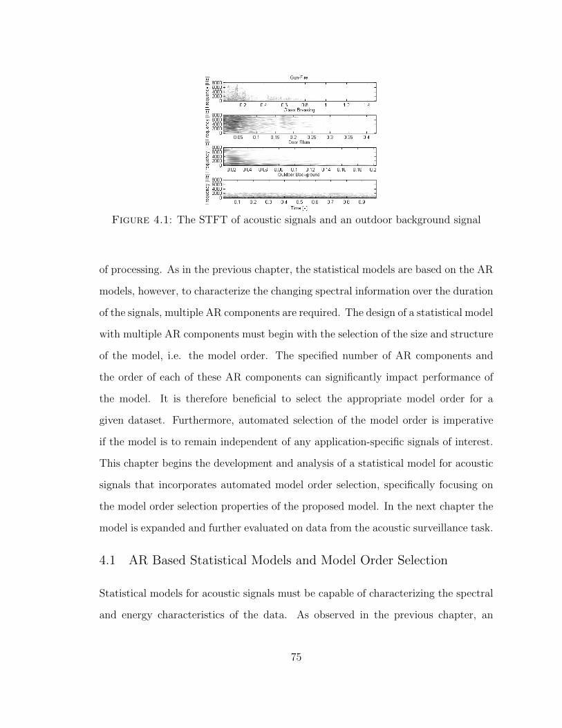
Figure 4.1: The STFT of acoustic signals and an outdoor background signal

of processing. As in the previous chapter, the statistical models are based on the AR

models, however, to characterize the changing spectral information over the duration

of the signals, multiple AR components are required. The design of a statistical model

with multiple AR components must begin with the selection of the size and structure

of the model, i.e. the model order. The specified number of AR components and

the order of each of these AR components can significantly impact performance of

the model. It is therefore beneficial to select the appropriate model order for a

given dataset. Furthermore, automated selection of the model order is imperative

if the model is to remain independent of any application-specific signals of interest.

This chapter begins the development and analysis of a statistical model for acoustic

signals that incorporates automated model order selection, specifically focusing on

the model order selection properties of the proposed model. In the next chapter the

model is expanded and further evaluated on data from the acoustic surveillance task.

4.1 AR Based Statistical Models and Model Order Selection

Statistical models for acoustic signals must be capable of characterizing the spectral

and energy characteristics of the data. As observed in the previous chapter, an

75

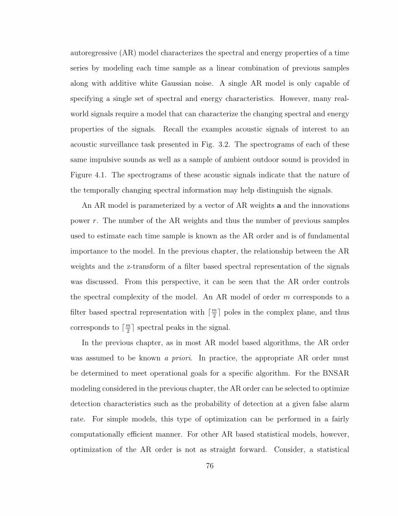
autoregressive (AR) model characterizes the spectral and energy properties of a time

series by modeling each time sample as a linear combination of previous samples

along with additive white Gaussian noise. A single AR model is only capable of

specifying a single set of spectral and energy characteristics. However, many real-

world signals require a model that can characterize the changing spectral and energy

properties of the signals. Recall the examples acoustic signals of interest to an

acoustic surveillance task presented in Fig. 3.2. The spectrograms of each of these

same impulsive sounds as well as a sample of ambient outdoor sound is provided in

Figure 4.1. The spectrograms of these acoustic signals indicate that the nature of

the temporally changing spectral information may help distinguish the signals.

An AR model is parameterized by a vector of AR weights a and the innovations

power r. The number of the AR weights and thus the number of previous samples

used to estimate each time sample is known as the AR order and is of fundamental

importance to the model. In the previous chapter, the relationship between the AR

weights and the z-transform of a filter based spectral representation of the signals

was discussed. From this perspective, it can be seen that the AR order controls

the spectral complexity of the model. An AR model of order m corresponds to a

filter based spectral representation with dm2e poles in the complex plane, and thus

corresponds to dm2e spectral peaks in the signal.

In the previous chapter, as in most AR model based algorithms, the AR order

was assumed to be known a priori. In practice, the appropriate AR order must

be determined to meet operational goals for a specific algorithm. For the BNSAR

modeling considered in the previous chapter, the AR order can be selected to optimize

detection characteristics such as the probability of detection at a given false alarm

rate. For simple models, this type of optimization can be performed in a fairly

computationally efficient manner. For other AR based statistical models, however,

optimization of the AR order is not as straight forward. Consider, a statistical

76

model consisting of s AR components. To optimize the AR order of each component,

considering M possible orders, performance must be evaluated for each of the sM

possible model structures. For hierarchical statistical models, such as the hidden

Markov models (HMMs) and mixture models considered in this work, selecting s can

be viewed as yet another model order selection problem. Simultaneous optimization

of s and the AR order for each component dramatically increases the number of

required performance evaluations beyond computational tractability.

The selection of an appropriate order for an AR model has been of interest to

the signal processing community for some time. The ability to quantify a model

order selection criterion was first approached by determining an ad hoc criterion that

aims to balance the fit of the model, typically the log-likelihood of the model, with

a penalty term that increases with the number of parameters. The most notable

of these criteria is the Akaike information criterion (AIC) [59] which has received

significant use due to its simplicity, but has also received criticism due to its ad hoc

nature [60]. A Bayesian approach to the model order selection problem typically

results in the need for approximate Bayesian inference. For example, use of the

Laplacian approximation for the posterior parameter density results in the Bayesian

information criterion (BIC) [60] which has also been widely used in model order

selection.

Both the AIC and BIC methods can be written in the form

log f (D|Mi)− P (ni, N) (4.1)

where ni is the number of free parameters to be estimated by model Mi, N is the

number of data points used for estimation, and P (·, ·) is a penalty term. To select

the best model order, the model with the maximum value of the AIC or BIC is

selected. To understand how these criterion function, note that the likelihood for

a model log f (D|Mi) typically increases with the number of parameters. However,

77

overly complex models do not generalized well to as yet unseen data. Therefore the

penalty term P (·, ·) increases with the number of free parameters to balance the

complexity and accuracy of the model. The AIC uses the simple penalty term ni,

independent of the number of data points, whereas the BIC derives the penalty term

ni logN from approximations and Bayesian methodology [61].

Similar to the performance based evaluation discussed above, information crite-

rion based methods for model order selection, like AIC and BIC, require learning

the parameters of the model for each of the model orders under consideration and

then evaluating the efficacy of each model using the specified criterion. Once again,

this methodology becomes computationally expensive especially when estimating the

order of AR models within a more sophisticated statistical model. For mixture or hid-

den Markov models utilizing AR model sources, the compound model order problem

creates an exponential increase in the number of models that must be constructed

and evaluated. Even if each AR component is restricted to having the same AR or-

der, a model must be constructed from every combination of AR order and number

of components under consideration.

Despite the difficulties associated with model order selection, hierarchical statis-

tical models utilizing AR models have been utilized for modeling time-series data

for a variety of tasks. In this chapter the focus is the mixture AR (MAR) model,

wherein a collection of AR components are used to create a non-linear model for

time-series data. In a MAR model, each time-sample has a corresponding latent

(hidden) variable zt that indicates from which of the AR components it originates.

Denoting the probability of obtaining a sample from AR component i as πi, the

probability density function for data at time t is

f (dt|ψt, a, r, m) =s∑i=1

πiNdt (a′iψt, ri) . (4.2)

where it has been assumed that there are s components each with an implied AR

78

order, mi.

Maximum likelihood learning for MAR models was first introduced in [62] and

the MAR model was later modified to incorporate heteroscedasticity [63], logistic AR

models [64], multivariate time-series [65], and AR moving average (ARMA) models

[66]. The learning procedure for each of these models is based on the expectation

maximization (EM) algorithm with a fixed number of mixture components and an

assumed AR order. In several of these MAR based models, most notably in [62], the

model order selection problem for MAR models is considered. In [62], a small scale

study for selecting the model order of a single MAR model with two components

with different AR orders in each of the components was considered using the AIC

and BIC criterion. Although the model order selection problem using AIC or BIC

requires exhaustive model estimation of each of the number of components and the

AR orders under consideration, [62] showed that the BIC is capable of determining

the correct model order provided a sufficient number of observations are available.

Bayesian parameter estimation for AR and MAR models has also been examined

[54, 67, 30, 55, 56]. In [67] a variational Bayesian (VB) learning procedure for an AR

model with a mixture of Gaussian innovations process is developed and model order

selection for the number of components in the innovations process and the AR order

is analyzed using the negative free energy (NFE). Similar to the model order selection

performed in [62], this approach requires parameter inference for each of the model

orders under consideration. The relation between Bayesian inference and automated

model order selection using the VB method was discussed briefly in Chapter 2. Recall

that the VB method maximizes the negative free energy

F (q (θ)) = Eq(θ)log f (D|θ) −KL (q (θ) ||f (θ)) . (4.3)

which is comprised of two terms, the average log-likelihood and a Kullback Leibler

divergence. These two terms have similar interpretation to the likelihood and penalty

79

terms used by information theoretic criterion. The model with the maximum NFE

can be selected in a manner similar to information criterion methods. Bayesian

learning procedures making use of the VB method for MAR and related models

are also presented in [30, 55, 56]. However, in each of these cases the number of

components in the mixture and the AR order are assumed known and the model

order selection problem is not addressed.

Statistical models utilizing a Dirichlet process (DP) prior provide automated

methods for model order selection within mixture models and HMMs by eliminating

the need to explicitly enumerate the number of components in a mixture model or

the number of states in an HMM [19, 68, 24]. DP based HMMs with AR sources

have been examined and successfully utilized for modeling time-series data [25, 69].

However, in both of these cases the AR order is assumed to be known. Although DP

priors provide solutions for automated model order selection for mixture models and

HMMs, they are insufficient for automated selection of the AR order. An automated

solution for selecting the AR order requires an alternate model formulation.

In several previous studies the order of regression coefficients is modeled as a

probabilistic quantity to create a probabilistic model that can be used to automat-

ically determine the appropriate order [70, 21, 20]. When used in an AR model

this formulation will be referred to as an uncertain-order AR (UOAR) model. In

these previous studies, UOAR or similar models have been used within hierarchical

statistical models to create more flexible models for time-series data. In [70] a time-

series is modeled as a sequence of UOAR models with discrete change points and

the number of change points and location of each change point must be determined.

In [21] and [20] mixture models with an uncertain number of UOAR components

are examined. Whereas [21] considers a discrete density over the number of mix-

ture components, [20] considers a DP mixture to construct an infinite mixture of

UOAR sources that has no specified maximum number of components, and provides

80

a principled approach to the model order selection problem within mixture models.

Each of these previous approaches offers a more sophisticated model for time-

series data through the use of Bayesian parameter estimation performed with Markov

chain Monte Carlo (MCMC) sampling. As mentioned in Chapter 2, MCMC sampling

techniques for approximate Bayesian inference are computationally and time inten-

sive, and lack a quantitative stopping criterion. As a result, the developed learning

procedures are inadequate for many signal processing applications that require rapid

parameter estimation or re-estimation, such as the acoustic sensing applications un-

der consideration in this work.

In this chapter a variational Bayesian (VB) learning procedure for the parameters

of DP mixtures of UOAR components is developed. This creates a more computa-

tionally efficient method for learning a non-linear time-series model that incorporates

automated model order selection. The model order selection accuracy of the model

is analyzed with respect to both the number of components in the mixture as well as

the AR order of each component and is considered more thoroughly than in previous

studies by analyzing AR models with random parameters.

Prior to development of this model however, the model order selection properties

of the UOAR model are compared to those provided by automatic relevance deter-

mination (ARD) [71] and to the common information criterion based techniques,

BIC and AIC. The comparison to ARD serves as a comparison to another Bayesian

framework capable of automatic AR order selection that can be included in more

complex statistical models. It is demonstrated that UOAR provides superior model

order selection performance and is more appropriate for inclusion in statistical models

making use of AR sources.

Following this, the VB learning procedure for the DP mixture of UOAR compo-

nents is developed and illustrated on synthetic data. The ability of UOAR models

to accurately determine the true AR order as well as the correct number of com-

81

ponents within MAR models is then analyzed and compared to MCMC inference

for DP mixtures of UOAR components similar to that developed in [20] and to VB

learning for DP mixtures of fixed-order AR components. The use of UOAR models

within MAR models is shown to provide superior performance over fixed order AR

models and the VB learning procedure for DP mixtures of UOAR models is shown to

have performance similar to that obtained using computationally intensive MCMC

inference. Therefore, the advantages of VB inference, specifically the parameterized

posterior density for tractable recursive Bayesian inference, can be obtained with

only minimal loss in model order selection accuracy.

Finally, to assess the efficacy of the VB learning procedure for DP mixtures of

UOAR models for acoustic signal modeling an acoustic surveillance task is analyzed.

A collection of anomalous signals that are of interest to the proposed classification

stage of acoustic sensing processing, such as muzzle blasts and door slams, is used as

an example to illustrate the ability of the algorithm to perform effectively on real-

world signals. The performance obtained using DP mixtures of UOAR models is

compared to MAR models with a fixed number of components with fixed AR orders.

The automated model order selection properties of the DP mixture of UOAR models

offers performance equivalent to the best performance obtained after a computation-

ally intensive search for the best number mixture components and AR order for fixed

MAR models.

4.2 Bayesian Inference for UOAR Models

Recall from the previous chapter that the AR likelihood function is

f (dt|ψt, a, r) = Ndt (a′ψt, r) (4.4)

and that the parameters can be efficiently estimated through the use of Bayesian

inference and the conjugate prior (CP) to the AR likelihood function, the Normal-

82

inverse-Wishart density. Using the same parameterization from the previous chapter,

the Normal-inverse-Wishart density is parameterized by an (m+ 1)×(m+ 1) matrix

V and scalar ν. Due to conjugacy with the AR likelihood function, the posterior

density for a set of data also follows a Normal-inverse-Wishart density with updated

hyperparameters. If the prior probability density is determined by hyperparameters

V0 and ν0 the posterior density has parameters determined by

V = V0 +T∑t=1

φtφ′t (4.5)

ν = ν0 + T (4.6)

where φt = [dt, ψ′t]′

and ψt = [dt−1, dt−2, . . . , dt−m]′. For simplicity in notation, in

the remainder of this work, it is assumed that the dataset has been truncated such

that φ1 corresponds to the first m samples of the dataset. Therefore the summa-

tion index in 4.5 differs from that in 3.30, however, the statements are equivalent.

From V and ν the mean and other marginal parameters for the AR weights and the

innovations power can be determined (see (3.19) and (3.20)). Note that this param-

eterization inherently assumes that the AR order m is fixed and thus certain. To

enable automated model order selection, uncertainty regarding the AR order must

be included into the model.

4.2.1 Bayesian Model Selection with Conjugate Priors

Recall that a CP for a given likelihood function results in an evidence calculation that

is analytically tractable. For example, for the AR likelihood function the evidence

is given by (3.36) with appropriate hyperparameters. When exact calculation of

the evidence is possible, posterior probabilities for a collection of models can be

determined using Bayes rule. Consider a collection of models Mi for 1 ≤ i ≤

M . Knowledge of these models is uncertain. Therefore, prior probabilities f (Mi)

83

(typically uniform over all models) are assigned and Bayesian inference is applied.

The posterior for model Mi is thus determined by

f (Mi|D) =f (D|Mi) f (Mi)∑M

m=1 f (D|Mm) f (Mm). (4.7)

Notice that the numerator is the evidence of modelMi and that the denominator is

the sum of the evidence for each model under consideration. Because the posterior

density for the models is discrete over a finite range, normalization (so that the

probabilities sum to unity) can be performed after calculation of each numerator.

Therefore it is only necessary to consider the posterior density

f (Mi|D) ∝ f (D|Mi) f (Mi) . (4.8)

By considering a uniform prior over models and taking the logarithm, the BIC can

be derived from this perspective.

Analytical determination of the posterior probabilities for a collection of models

requires calculation of the evidence for each model. Because analytic calculation of

the evidence is typically only possible when using CPs, it follows that analytic model

selection is only possible when all models under consideration are accompanied by

their CPs. This fact will be exploited to perform model order selection in AR models.

4.2.2 Uncertain-Order AR Models

Model order selection for AR models is accomplished by considering AR models with

varying orders. Consider the AR likelihood function conditional on the implied order

of the model m taking the value i

f(dt|ψi

t, ai, r,m = i

)= Ndt|m=i

((ai)′ψit, r)

(4.9)

In (4.9) and throughout the remainder of this chapter, superscripts are used to

indicate the dependence of a quantity on the AR order, and thus indicate the vector

84

or matrix size. Model order selection is accomplished by performing Bayesian model

selection by considering a range of AR orders from 1 to M . The maximum AR

length M can be selected for a given dataset to enforce physical constraints or from

computational considerations. Since each of the M models are AR, the prior for each

model is chosen to be the CP, the Normal-inverse-Wishart density. Therefore, for

AR order m = i the prior density of the AR weights and the innovations power is

f (a, r|m = i) = N iWa,r|m=i

(Vi

0, νi0

). (4.10)

The posterior probability for each model can be found using (4.8) and (3.36). The

probability of each model f (Mi) is now equivalent to the probability of the AR

order taking value i. A prior probability f (m = i) is assigned to each order and the

posterior is determined as follows

f (m = i|D) ∝ f (m = i) f (D|m = i)

= f (m = i)

∫f (D|m = i, a, r) f (a, r|m = i) dadr

= f (m = i)

∫ T∏t=1

Ndt|m=i

((ai)′ψit, r

i)N iWa,r|m=i

(Vi

0, νi0

)daidri.

(4.11)

To determine the value of the integration, consider calculation of the posterior

Normal-inverse-Wishart parameters for AR order i which is known to be

N iWa,r|m=i

(Vi, νi

)=

∏Tt=1Ndt|m=i

((ai)

′ψit, r

i)N iWa,r|m=i (V

i0, ν

i0)∫ ∏T

t=1Ndt|m=i

((ai)′ψi

t, ri)N iWa,r|m=i (Vi

0, νi0) daidri

.

(4.12)

Therefore, the required integration is the ratio of the Normal-inverse-Wishart densi-

ties ∏Tt=1Ndt|m=i

((ai)

′ψit, r

i)N iWa,r|m=i (V

i0, ν

i0)

N iWa,r|m=i (Vi, νi)(4.13)

85

From (3.23 - 3.28) it can be seen that the numerator can be rewritten as

(2π)12(νi−νi0) Z (Vi, νi)

Z (V0, ν0)N iWa,r|m=i

(Vi, νi

). (4.14)

If all of the model orders share the same value for ν0 the leading term can be ignored

and the integral can be replaced by the ratio of the two normalizing constants.

Therefore, the posterior density for model i can be written as

f (m = i|D) ∝ f (m = i)Z (Vi, νi)

Z (Vi0, ν

i0)

(4.15)

After calculating (4.15) for 1 ≤ i ≤ M , the posterior density for m can then be

obtained through normalization.

Therefore, analytic Bayesian AR order selection is accomplished by first deter-

mining the hyperparameters for each of the M posterior Normal-inverse-Wishart

posterior densities and subsequently determining the posterior probability for each

AR order using (4.15). This calculation is exact given its assumptions and can be cal-

culated rapidly. Although this method was derived from the perspective of Bayesian

model selection it is equivalent to considering the AR order a random parameter of

a generative model. Consider a generative process in which, first m is drawn from a

discrete density, then AR weights and innovations powers are drawn from a Normal-

inverse-Wishart density given m and finally data is drawn from an AR model using

the drawn AR weights and innovations power. If f (m = i) for 1 ≤ i ≤M is denoted

as a probability mass vector µ, this generative process can be written as follows

m ∼ Discrete (µ, [1, . . . ,M ])

a, r|m ∼ N iWa,r (vm,Vm)

dt ∼ Ndt (a′ψt, r) . (4.16)

This is the viewpoint that leads to the name uncertain-order AR (UOAR) model.

Since a discrete density is assumed over m, the prior density for this model is referred

86

to as a discrete-Normal-inverse-Wishart.

f (a, r,m = i) = f (m = i) f (a, r|m = i)

= µiN iWa,r|m=i

(Vi, νi

)(4.17)

The density is determined by M sets of Normal-inverse-Wishart hyperparameters,

Vi, νii=1,...,M and the vector of AR order probabilities µ.

Utilization of this prior for AR parameters infers the model order from the data

in a computationally efficient manner without approximation given the assumptions.

The UOAR model provides a parameterized posterior density for the AR order, mak-

ing UOAR models appropriate for use with larger, more complex statistical models,

such as mixture models. The UOAR model can be compared to another Bayesian

model that performs a type of model order selection, the automatic relevance de-

termination (ARD) model [72, 71]. For regression problems, ARD ensures that the

means of the posterior density for regression weights that would be small non-zero

values using typical regression techniques are identically zero. In many linear regres-

sion problems this is an acceptable form of model order selection since the regressors

are exchangeable in order. For AR models the regression weights are not exchange-

able in order and the weights have a physical meaning with regards to the frequency

spectrum of the time-series. Therefore, the task of selecting the AR order is sub-

stantially different than the task for which ARD is intended.

Despite this, an ARD prior can be used to estimate AR weights and thus be used

within larger statistical models. This approach is take in [26], wherein an ARD prior

is used as a prior for AR weights within an HMM with parameter inference done

using MCMC sampling. In the following section, the model order selection accuracy

of ARD is compared to the UOAR prior as well as to common information criterion

based approaches. As a prior formulation to be used within larger statistical models

such as the DP mixtures considered in Section 4.4, an ARD prior is an alternative

87

choice to the UOAR prior. The accuracy and computational requirements of each

prior will determine the appropriate formulation for our purposes.

4.3 AR Model Order Selection Experiment

The model order selection accuracy of the UOAR model is now compared to the

ARD prior formulation as well as the most common information criterion based

approaches, AIC and BIC. The comparison between the UOAR model and the ARD

formulation will illustrate why the UOAR formulation is selected for use within DP

mixture models of AR sources discussed in Section 4.4. The comparison to AIC and

BIC provides a baseline performance against established techniques.

Each model order selection method is applied to a synthetic data set comprised

of data generated with known AR parameters. The estimation performance of each

algorithm is then analyzed as a function of the number of samples used for parame-

ter estimation as well as the length of the AR model. Each true AR model contains

randomly generated parameters to eliminate dependence on particular AR param-

eters. This is a departure from most previous investigations of AR order selection

techniques in which only specific AR models or datasets were analyzed.

A kth order AR model can be characterized by the roots of the equation formed

by the AR weights [53]

1−k∑i=1

aiz−i = 0. (4.18)

The set of k solutions to this equation, Riejθi , 1 ≤ i ≤ k, describe the spectral

characteristics of data generated from the AR model. Stable, or stationary, AR

models have all of the k roots inside of the unit circle in the complex plane, |Ri| < 1.

The k roots are sets of complex conjugate pairs with an additional single real valued

root for AR models with odd order. AR models with random parameters can be

88

generated by drawing bk2c sets of magnitude and angles for the complex conjugate

pairs of roots, Rie±jθi , 1 ≤ i ≤ bk

2c, and, if necessary, a single real root. The

AR weights can then be found by determining the coefficients of the polynomial

corresponding to the specified roots.

One thousand time series were generated for each k ∈ 1, 2, 3, 4, with dataset

instantiations of 25, 50, 100, 250, and 500 samples. To ensure that the generated

parameters govern a stable AR model with strong spectral peaks the magnitude of

the roots was drawn from a uniform distribution between 0.98 and 0.99 and the

angles of the roots were drawn uniformly between 0.1π and 0.9π.

Each model order selection method is then applied to each synthetically generated

time series and an estimate of the AR order is determined. Parameters of each of

the techniques were set to allow the maximum allowable selected AR order to be

20. The AIC and BIC methods calculate the maximum likelihood estimates of the

parameters of the AR model and the innovations power for each order, estimate the

likelihood of the observed data for the estimated parameters, and subtract a penalty

term that increases with AR length. The AR order with the largest metric is then

selected. As stated previously, the ARD method does not seek to minimize the AR

order but rather seeks to force irrelevant AR weights to zero, and as a result, judging

the ability of ARD to determine the AR order requires a method to determine the

resulting AR order. For this experiment a threshold of 0.01 was set and the regression

weight above this value corresponding to the earliest time sample was used as the

AR order. Because this arbitrary step is necessary to evaluate the ARD method

caution should be taken when interpreting the results as these results are sensitive

to the threshold that was selected. The UOAR model provides a discrete probability

density for the AR order. For evaluation, the mode of this density is taken as the

selected AR order.

Fig. 4.2 provides the histograms of the estimated AR orders for the each of

89

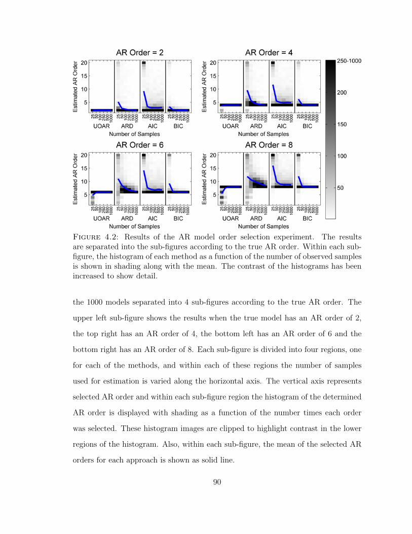
Figure 4.2: Results of the AR model order selection experiment. The resultsare separated into the sub-figures according to the true AR order. Within each sub-figure, the histogram of each method as a function of the number of observed samplesis shown in shading along with the mean. The contrast of the histograms has beenincreased to show detail.

the 1000 models separated into 4 sub-figures according to the true AR order. The

upper left sub-figure shows the results when the true model has an AR order of 2,

the top right has an AR order of 4, the bottom left has an AR order of 6 and the

bottom right has an AR order of 8. Each sub-figure is divided into four regions, one

for each of the methods, and within each of these regions the number of samples

used for estimation is varied along the horizontal axis. The vertical axis represents

selected AR order and within each sub-figure region the histogram of the determined

AR order is displayed with shading as a function of the number times each order

was selected. These histogram images are clipped to highlight contrast in the lower

regions of the histogram. Also, within each sub-figure, the mean of the selected AR

orders for each approach is shown as solid line.

90

From Fig. 4.2 it can be seen that both the BIC and UOAR techniques determine

the correct AR order with high fidelity, as indicated by the dark region of each

histogram at the correct AR order. When a smaller amount of data is used for

estimation, the BIC becomes less accurate and overestimates the AR order. This is

more prevalent when the true AR order is larger, as seen in the bottom sub-figures.

The UOAR technique also becomes less accurate when fewer samples are used for

estimation, however, the UOAR model tends to underestimate the AR order. The

accuracy of both methods are due to their origins in Bayesian analysis. The BIC

makes use of the Laplacian approximation for the posterior parameter density to

arrive a computational simple expression for model order selection [31]. The UOAR

prior works in a similar manner but instead uses the discrete-Normal-inverse-Wishart

density as the prior and posterior density for the parameters. As a result the UOAR

model is a more attractive choice for inclusion in larger statistical models as it is

more amenable to Gibbs sampling and VB inference.

The other two methods, the AIC and ARD, do not accurately estimate the AR

order. The AIC tends to over estimate the AR order in nearly all cases with the

degree of over estimation reducing as the number of samples increases. This is due

to inaccuracy in the ad hoc penalty term employed by the AIC [73]. The ARD prior

also does not accurately estimate the AR order, particularly with limited data. As

stated above, ARD does not seek to determine the AR order and as a result an ad

hoc technique was needed to determine the estimated AR order from the determined

regression weights. An alternate selection of the threshold used for determining the

AR order as well as the prior parameters for the ARD model could alter these results.

The prior parameters and the ad hoc method for determining the AR order are not

the only factors contributing to the poor performance of the ARD prior based model

order selection. The ARD prior requires an iterative learning procedure to estimate

the parameters of the model. The variational Bayesian formulation from [61] was

91

used for these simulations. The VB learning procedure is an optimization procedure

that is not guaranteed to find the global maximum. Instead, a local maximum may

be found depending on the initialization of the parameters. As is standard practice

for the ARD prior, for these simulations the parameters were initialized using the

least squares solution using all of the regressors, corresponding to the maximum

AR order. Using this initialization the local solution reached by the VB learning

procedure does not always determine the correct AR order. This becomes more

prevalent with a smaller amount of data and more complex models (AR order of 8).

VB learning for the ARD prior was considered in this work instead of other learn-

ing procedures (for example [71]) as our primary interest is performing variational

inference of DP mixture with AR sources. In addition to the poor model selection

performance of the ARD method there is another reason that it may not be the best

choice for inclusion within larger statistical models. Variational inference for models

with ARD priors is known to have slow convergence rate and thus require a large

number of iterations to converge to a sparse solution [74]. Although the methods

presented in [74] can greatly reduce the number of required iterations there is still a

large computational burden associated with variational inference with ARD priors.

The poor model selection performance and the increased computational require-

ments of the ARD method indicate the UOAR prior formulation as a more appro-

priate choice for inclusion within larger statistical models. In the remainder of this

chapter we analyze the use of the UOAR prior within DP mixture models to create

a more expressive statistical model than a single AR model.

4.4 Dirichlet Process Mixtures of UOAR Models

As mentioned previously, a model utilizing a single AR source is not capable of

characterizing the changing spectral and energy content observed in many real-world

signals and thus reliable statistical modeling of these types of time-series requires

92

a more sophisticated model. A more expressive model for time-series data can be

realized by considering a mixture of AR (MAR) models. A MAR model with C

components has the likelihood function

f (dt|ψt, a, r) =C∑i

πiNdt (a′iψt, ri) . (4.19)

Models of this type have been considered previously [62, 30, 55, 56], however, select-

ing the appropriate AR order and number of components C for these models is a

significant computational challenge.

As seen in the experiment in Section 4.2, an UOAR prior can determine the

correct AR order to a reasonable degree of accuracy while simultaneously remaining

conjugate to the AR likelihood function. Therefore, the UOAR prior provides a

means of automatically determining the AR order of components within a larger

statistical model such as a mixture model. Similarly, a mixture model utilizing

a Dirichlet process (DP) prior can provide a means of automatically determining

the number of components within a probabilistic mixture model. Thus, UOAR

models within DP mixture models create expressive models for time-series data that

automatically perform both of the model order selection problems.

A DP mixture of UOAR model components has previously been considered in

[20], however, the parameters of the DP mixture model were learned using MCMC

techniques. As mentioned previously, MCMC inferences is computationally intensive,

lacks a quantitative stopping criterion and results in a posterior density comprised of

numerical samples. For the acoustic sensing applications of interest to this research

a computationally efficient algorithm that is capable of rapid inference is required.

Furthermore, it is desired that the form of the posterior density be amenable to

recursive Bayesian inference. In this section we develop a VB learning procedure for

DP mixtures UOAR models to provide a computationally tractable solution to AR

based time series modeling that incorporates automated model order selection.

93

4.4.1 Dirichlet Process Mixtures

The DP is a probability density function for probability density functions [19]. When

used in conjunction with mixture models, the DP provides a method to automati-

cally determine the appropriate number of components [68]. Initially, learning for DP

mixture models was accomplished by utilizing MCMC techniques [75, 76] and these

methods have been adapted to include UOAR models [20]. More recently, VB learn-

ing procedures for DP mixtures have been introduced [77, 78, 79, 80]. The coupling

of VB learning procedures with DP priors has introduced tractable solutions to the

model order selection problem associated with selecting the number of components

within a probabilistic mixture model.

A DP is defined by a base measure, G0, and a scaling parameter, α. A random

draw from the DP is a measure G and a set of random draws from G, θi, 1 ≤ i ≤ N

exhibit clustering properties known as a Polya urn scheme [81]. This implies that

some of the θi will have identical values and that the draw from the DP, G, is

(almost surely) discrete. Drawing from a Polya urn scheme is typically referred to

as a Chinese restaurant process (CRP) due to analogy made with way patrons sit

when entering a restaurant in China. Consider a restaurant with an infinite number

of tables, each with an infinite number of available seats. When each customer

enters the restaurant he/she sits at a table with probability proportional to the

number of people already sitting at each table but with some other small probability

(proportional to α) he/she will choose to sit at the first empty table they come to.

More specifically, if table i has ηi people already sitting at it and there are N total

people in the restaurant patron j will sit at table i with probability ηiN+α

and will sit

at an empty table with probability αN+α

. As more patrons enter the restaurant the

total number of tables in use stabilizes with a few tables having most of the people

sitting at them. The amount of total tables in use is related to α. A larger value for

94

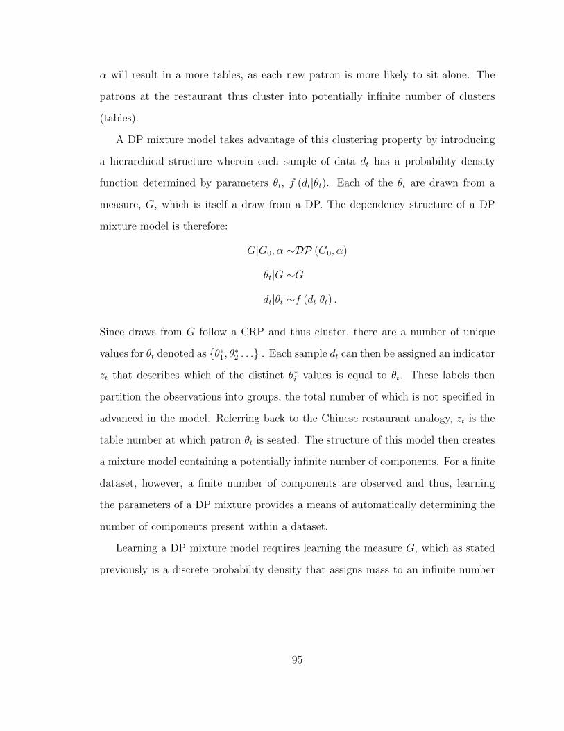
α will result in a more tables, as each new patron is more likely to sit alone. The

patrons at the restaurant thus cluster into potentially infinite number of clusters

(tables).

A DP mixture model takes advantage of this clustering property by introducing

a hierarchical structure wherein each sample of data dt has a probability density

function determined by parameters θt, f (dt|θt). Each of the θt are drawn from a

measure, G, which is itself a draw from a DP. The dependency structure of a DP

mixture model is therefore:

G|G0, α ∼DP (G0, α)

θt|G ∼G

dt|θt ∼f (dt|θt) .

Since draws from G follow a CRP and thus cluster, there are a number of unique

values for θt denoted as θ∗1, θ∗2 . . . . Each sample dt can then be assigned an indicator

zt that describes which of the distinct θ∗i values is equal to θt. These labels then

partition the observations into groups, the total number of which is not specified in

advanced in the model. Referring back to the Chinese restaurant analogy, zt is the

table number at which patron θt is seated. The structure of this model then creates

a mixture model containing a potentially infinite number of components. For a finite

dataset, however, a finite number of components are observed and thus, learning

the parameters of a DP mixture provides a means of automatically determining the

number of components present within a dataset.

Learning a DP mixture model requires learning the measure G, which as stated

previously is a discrete probability density that assigns mass to an infinite number

95

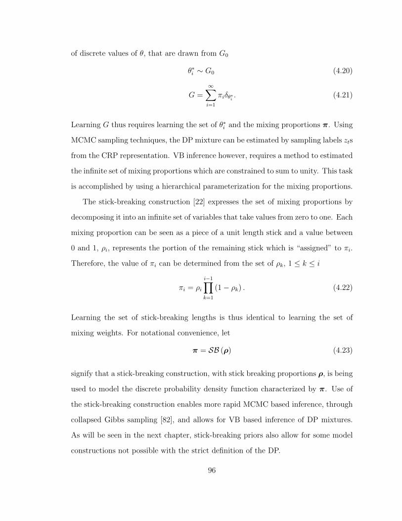
of discrete values of θ, that are drawn from G0

θ∗i ∼ G0 (4.20)

G =∞∑i=1

πiδθ∗i . (4.21)

Learning G thus requires learning the set of θ∗i and the mixing proportions π. Using

MCMC sampling techniques, the DP mixture can be estimated by sampling labels zts

from the CRP representation. VB inference however, requires a method to estimated

the infinite set of mixing proportions which are constrained to sum to unity. This task

is accomplished by using a hierarchical parameterization for the mixing proportions.

The stick-breaking construction [22] expresses the set of mixing proportions by

decomposing it into an infinite set of variables that take values from zero to one. Each

mixing proportion can be seen as a piece of a unit length stick and a value between

0 and 1, ρi, represents the portion of the remaining stick which is “assigned” to πi.

Therefore, the value of πi can be determined from the set of ρk, 1 ≤ k ≤ i

πi = ρi

i−1∏k=1

(1− ρk) . (4.22)

Learning the set of stick-breaking lengths is thus identical to learning the set of

mixing weights. For notational convenience, let

π = SB (ρ) (4.23)

signify that a stick-breaking construction, with stick breaking proportions ρ, is being

used to model the discrete probability density function characterized by π. Use of

the stick-breaking construction enables more rapid MCMC based inference, through

collapsed Gibbs sampling [82], and allows for VB based inference of DP mixtures.

As will be seen in the next chapter, stick-breaking priors also allow for some model

constructions not possible with the strict definition of the DP.

96

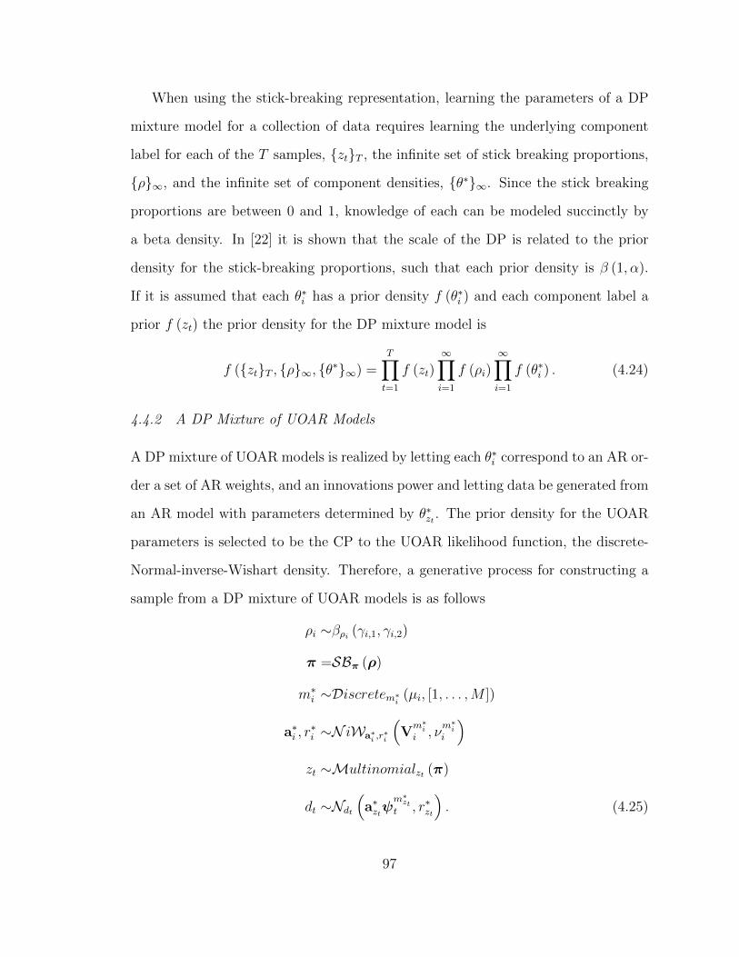
When using the stick-breaking representation, learning the parameters of a DP

mixture model for a collection of data requires learning the underlying component

label for each of the T samples, ztT , the infinite set of stick breaking proportions,

ρ∞, and the infinite set of component densities, θ∗∞. Since the stick breaking

proportions are between 0 and 1, knowledge of each can be modeled succinctly by

a beta density. In [22] it is shown that the scale of the DP is related to the prior

density for the stick-breaking proportions, such that each prior density is β (1, α).

If it is assumed that each θ∗i has a prior density f (θ∗i ) and each component label a

prior f (zt) the prior density for the DP mixture model is

f (ztT , ρ∞, θ∗∞) =T∏t=1

f (zt)∞∏i=1

f (ρi)∞∏i=1

f (θ∗i ) . (4.24)

4.4.2 A DP Mixture of UOAR Models

A DP mixture of UOAR models is realized by letting each θ∗i correspond to an AR or-

der a set of AR weights, and an innovations power and letting data be generated from

an AR model with parameters determined by θ∗zt . The prior density for the UOAR

parameters is selected to be the CP to the UOAR likelihood function, the discrete-

Normal-inverse-Wishart density. Therefore, a generative process for constructing a

sample from a DP mixture of UOAR models is as follows

ρi ∼βρi (γi,1, γi,2)

π =SBπ (ρ)

m∗i ∼Discretem∗i (µi, [1, . . . ,M ])

a∗i , r∗i ∼N iWa∗i ,r

∗i

(Vm∗ii , ν

m∗ii

)zt ∼Multinomialzt (π)

dt ∼Ndt(a∗ztψ

m∗ztt , r∗zt

). (4.25)

97

4.4.3 Variational Bayesian Inference for DP Mixtures

As the required posterior integration is intractable, Bayesian inference for DP mix-

ture requires approximation. Furthermore, an additional approximation is necessary

for the infinite sets of parameters. Variational learning for DP mixtures was first

introduced using the truncated stick breaking technique in [77] and [78] and later

modified to the tied stick breaking technique in [80]. The two techniques differ in

the method that is used to approximate the infinite number of components. Both

techniques assume that there is a maximum number of components that can be es-

timated, K. The truncated stick representation assumes that only K components

exist in the mixture while the tied stick breaking representation assumes that all

mixture components greater than K have densities equal to the prior. The tied stick

breaking representation provides a more accurate approximation that allows for more

robust estimation of DP mixture models, and is utilized in this research.

The variational Bayesian formulation for DP mixtures from [78] assumes that the

posterior density for each stick breaking proportion is a beta distribution q (ρi) =

β (γi,1, γi,2), each label is modeled as a discrete probability distribution q (zt = i),

and the probability density for the parameters of the ith component, θ∗i , is modeled

with a density from the dynamic exponential family, q (θ∗i ), typically conjugate to

the likelihood function. Therefore, the approximate posterior density of interest is

q (ρK , θK , ztT ) =K∏k=1

q (ρk)K∏k=1

q (θ∗k)T∏t=1

q (zt) (4.26)

and the hyperparameters defining each of these densities must be determined.

Application of the VB method to this formulation results in update equations

for each of the hyperparameters. The update equations for hyperparameters for ρi

and zt can be defined in terms of a general observation model defined by parameters

θ [77, 78, 80]. Recall that for the DP mixture UOAR components, θ∗ corresponds

98

to the set of UOAR parameters and that q (θ∗i ) are discrete-Normal-inverse-Wishart

densities. First the hyperparameter update equations for ρi and zt will be determined

in general and the necessary quantities to specifiy a DP mixture UOAR components

will be identified. Then these quantities will be derived from the UOAR model.

Calculation of q (zt) is facilitated by the definition

St,i = Eq(ρ)log f (zt = i|ρ)+ Eq(θ∗i )log f (dt|θ∗i ) (4.27)

for each observation t and component label i. The first term of (4.27) is determined

by using (4.22) and known moments of the beta density.

Eq(ρ)log f (zt = i|ρ) = Ψ (γi,1)−Ψ (γi,1 + γi,2) +i−1∑k=1

(Ψ (γk,2)−Ψ (γk,1 + γk,2))

(4.28)

In (4.28) Ψ (·) is the digamma function (see B). The second term of (4.27) is specific

to the observation model under consideration. For the UOAR model discussed in

this work this quantity is discussed in detail in the next section.

Using St,i the discrete density for the component labels can be determined by

q (zt = i) =exp (St,i)∑∞k=1 exp (St,k)

(4.29)

where the infinite sum in the denominator is calculated using the tied stick breaking

technique presented in [80]. Using q (zt = i) the update equations for the hyperpa-

rameters of the stick breaking proportions can be determined.

γi,1 = 1 +T∑t=1

q (zt = i) (4.30)

γi,2 = α +T∑t=1

∞∑k=i+1

q (zt = k) (4.31)

From (4.30) and (4.31) it can be seen that a β (1, α) prior has been assigned to each

stick proportion. This is by definition of the DP [82]. A G (ω1, ω2) prior is placed on

the value of α as described in [78].

99

Iteratively using these equations to update the hyperparameters for the stick

breaking proportions and the component labels as well as the hyperparameters gov-

erning each θ∗i (discussed below for UOAR models) is equivalent to an iterative

maximization of the negative free energy. The value of the negative free energy is

used to monitor convergence of the learning procedure.

F =T∑t=1

log∞∑i=1

exp (St,i)

−K∑k=1

KL (q (ρk) |f (ρk))

−K∑k=1

KL (q (θk) |f (θk)) (4.32)

Once again, the infinite sum of the first term is calculated using the tied stick breaking

representation presented in [80]. The second and third terms are the KL divergence

between the posterior and prior parameters for the stick breaking proportions and

the source densities respectively. The KL divergence for the source densities must

be determined for the particular model under consideration. The KL divergence for

the discrete-Normal-inverse-Wishart density used as the prior and posterior density

for the UOAR model is discussed in the next section.

4.4.4 Variational Bayesian Inference for DP Mixtures of UOAR Models

Learning the parameters of a DP mixture model of UOAR sources can be accom-

plished by utilizing the above model for DP mixtures along with the discrete-Normal-

inverse-Wishart prior for UOAR model discussed in Section 4.2. Using the notation

above, each θ∗k is a set of AR weights with unkown order and an innovations power.

A discrete-Normal-inverse-Wishart density is then used as the prior density for each

θ∗k. From the above discussion of DP mixtures, three quantities must be determined

when using a discrete-Normal-inverse-Wishart density for θ∗k and the AR likelihood

100

function: the expected value of the log of UOAR model likelihood function with

respect to the posterior source distribution (the second term of (4.27)), the hyper-

parameter update equations for the UOAR model, and the KL divergence between

discrete-Normal-inverse-Wishart densities, to be used in the calculation of the nega-

tive free energy.

The expected value of the log of UOAR model likelihood function with respect

to the posterior source distribution, the second term of (4.27), for the UOAR model,

can be determined by taking the expected value of the logarithm of (4.9),

Eq(m,a,r)log f (dt|ψt,m, a, r) =M∑i=1

q (m = i)Eq(a,r|m=i)log f(dt|ψi

t, ai, r).

(4.33)

Taking the expected value of the UOAR likelihood function conditioned on the AR

order can be determined from and several moments of the Normal-inverse-Wishart

density given in [30]

Eq(a,r|m=i)log f(dt|ψi

t, ai, r) = −1

2log π − 1

2Ψ

(ν − i− 2

2

)

− 1

2log λi − 1

2ψi′t

(Viaa

)−1ψit −

(ν − i− 2)

2λi(dt − ai′ψi

t

)2. (4.34)

In (4.34) the values of λ and Vaa are defined as in (3.17) and (3.21) and a = V−1aa Va1.

Using (4.33) and (4.34) the second term of (4.27) can be determined when using

UOAR components.

The second quantity required for the DP mixture of UOAR components is the

set of update equations for the hyperparameters governing the source parameter

density a specific component. These update equations can be determined using the

VB method to maximize the negative free energy given the hyperparameters for the

other model parameters. Noting that the posterior probability of sample t belonging

to component i is q (zt = i) the hyperparameter update equations for the component

101

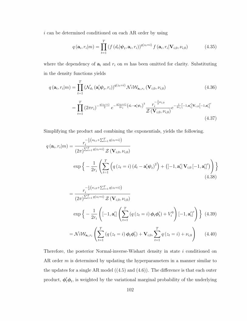
i can be determined conditioned on each AR order by using

q (ai, ri|m) =T∏t=1

(f (dt|ψt, ai, ri))q(zt=i) f (ai, ri|Vi,0, νi,0) (4.35)

where the dependency of ai and ri on m has been omitted for clarity. Substituting

in the density functions yields

q (ai, ri|m) =T∏t=1

(Ndt (a′iψt, ri))q(zt=i)N iWai,ri (Vi,0, νi,0) (4.36)

=T∏t=1

(2πri)− q(zt=i)

2 e− q(zt=i)

2ri(dt−a′iψt)

2 r− 1

2νi,0

i

Z (Vi,0, νi,0)e− 1

2ri[−1,a′i]Vi,0[−1,a′i]

′

(4.37)

Simplifying the product and combining the exponentials, yields the following.

q (ai, ri|m) =r− 1

2(ν0,i+∑Tt=1 q(zt=i))

i

(2π)∑Tt=1 q(zt=i)Z (Vi,0, νi,0)

exp− 1

2ri

(T∑t=1

(q (zt = i) (dt − a′iψt)

2)

+([−1, a′i] Vi,0 [−1, a′i]

′))(4.38)

=r− 1

2(νi,0+∑Tt=1 q(zt=i))

i

(2π)∑Tt=1 q(zt=i)Z (Vi,0, νi,0)

exp− 1

2ri

([−1, a′i]

(T∑t=1

(q (zt = i)φtφ′t) + V 0

i

)[−1, a′i]

′

)(4.39)

= N iWai,ri

(T∑t=1

(q (zt = i)φtφ′t) + Vi,0,

T∑t=1

q (zt = i) + νi,0

)(4.40)

Therefore, the posterior Normal-inverse-Wishart density in state i conditioned on

AR order m is determined by updating the hyperparameters in a manner similar to

the updates for a single AR model ((4.5) and (4.6)). The difference is that each outer

product, φ′tφt, is weighted by the variational marginal probability of the underlying

102

component and ν is no longer the number of samples but is now the expected number

of samples belonging to component i determined by the sum of q (zt = i) over all

observations.

Updating the hyperparameters for an UOAR model within a mixture model is

accomplished by first updating the Normal-inverse-Wishart density for each compo-

nent and each AR order. For completeness, now showing the dependency on the AR

order m, the each of the Normal-inverse-Wishart hyperparameters are updated as

follows

Vmi = Vm

0 +T∑t=1

q (zt = i)φmt (φmt )′ (4.41)

νm = νm0 +T∑t=1

q (zt = i) . (4.42)

Using these equations, the hyperparameters for the Normal-inverse-Wishart condi-

tioned on each AR order from 1 to M can be determined. The discrete posterior

density for the AR order can then be determined by using these values with (4.15).

This will yield all of the necessary hyperparameter update equations for the UOAR

model.

The final quantity needed for the VB learning procedure is the KL divergence

between the prior and posterior discrete-Normal-inverse-Wishart densities governing

the parameters of the UOAR model. This is required for the calculation of the

negative free energy (4.32). This quantity can be expressed by conditioning on the

AR order and taking the expected value over the density for the AR order.

KL (q (m, a, r) ||f (m, a, r)) =∑i

q (m = i) KL (q (a, r|m = i) ||f (a, r|m = i))

+ KL (q (m) ||f (m)) (4.43)

The terms of this equation are KL divergence between two Normal-inverse-Wishart

densities (given in Appendix A) and the KL divergence between two discrete densi-

103

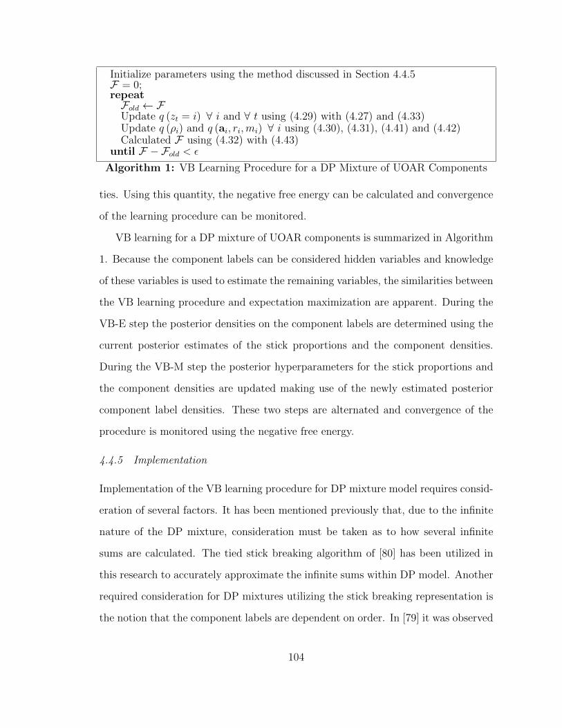
Initialize parameters using the method discussed in Section 4.4.5F = 0;repeatFold ← FUpdate q (zt = i) ∀ i and ∀ t using (4.29) with (4.27) and (4.33)Update q (ρi) and q (ai, ri,mi) ∀ i using (4.30), (4.31), (4.41) and (4.42)Calculated F using (4.32) with (4.43)

until F − Fold < ε

Algorithm 1: VB Learning Procedure for a DP Mixture of UOAR Components

ties. Using this quantity, the negative free energy can be calculated and convergence

of the learning procedure can be monitored.

VB learning for a DP mixture of UOAR components is summarized in Algorithm

1. Because the component labels can be considered hidden variables and knowledge

of these variables is used to estimate the remaining variables, the similarities between

the VB learning procedure and expectation maximization are apparent. During the

VB-E step the posterior densities on the component labels are determined using the

current posterior estimates of the stick proportions and the component densities.

During the VB-M step the posterior hyperparameters for the stick proportions and

the component densities are updated making use of the newly estimated posterior

component label densities. These two steps are alternated and convergence of the

procedure is monitored using the negative free energy.

4.4.5 Implementation

Implementation of the VB learning procedure for DP mixture model requires consid-

eration of several factors. It has been mentioned previously that, due to the infinite

nature of the DP mixture, consideration must be taken as to how several infinite

sums are calculated. The tied stick breaking algorithm of [80] has been utilized in

this research to accurately approximate the infinite sums within DP model. Another

required consideration for DP mixtures utilizing the stick breaking representation is

the notion that the component labels are dependent on order. In [79] it was observed

104

that reordering the component labels so that components are order in decreasing size

results in more robust learning of DP mixture models. As a result this technique has

also been utilized in this research.

A practicality of most optimization procedures including VB is the need to prop-

erly initialize the algorithm, which helps the optimization procedure to avoid local

maxima. The required initialization procedure for a DP mixture model is dependent

on the component density under consideration. For the UOAR mixture model an

initialization procedure based on K-means clustering [83] of many sets of maximum

likelihood estimated AR weights and innovations powers seems to provide robust

initialization.

In particular, to initialize the algorithm, the time-series data from which the

parameters of the model are being estimated is partitioned into frames. An ad hoc

frame length of 100 samples was selected. In each of these frames the maximum

likelihood estimates for AR weights and innovations powers are determined using an

AR order of M . This collection of weights and innovations powers is then treated as

an M+1 dimensional dataset and K-Means clustering is performed using K clusters.

These cluster assignments are then used to set the initial component membership

probabilities for each sample and component, q (zt = i) and from the component

membership probabilities the hyperparameters for each component density as well

as the stick breaking proportions can be determined.

When analyzing the results of the learned DP mixture it is often convenient to

determine the number of components that have non-negligible proportion weights.

After the completion of the learning procedure, components having a proportion

weight less than 0.01 are removed from the model and the remaining proportion

weights are adjusted accordingly.

105

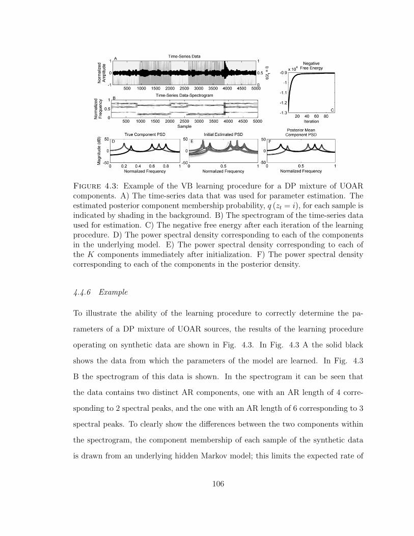
Figure 4.3: Example of the VB learning procedure for a DP mixture of UOARcomponents. A) The time-series data that was used for parameter estimation. Theestimated posterior component membership probability, q (zt = i), for each sample isindicated by shading in the background. B) The spectrogram of the time-series dataused for estimation. C) The negative free energy after each iteration of the learningprocedure. D) The power spectral density corresponding to each of the componentsin the underlying model. E) The power spectral density corresponding to each ofthe K components immediately after initialization. F) The power spectral densitycorresponding to each of the components in the posterior density.

4.4.6 Example

To illustrate the ability of the learning procedure to correctly determine the pa-

rameters of a DP mixture of UOAR sources, the results of the learning procedure

operating on synthetic data are shown in Fig. 4.3. In Fig. 4.3 A the solid black

shows the data from which the parameters of the model are learned. In Fig. 4.3

B the spectrogram of this data is shown. In the spectrogram it can be seen that

the data contains two distinct AR components, one with an AR length of 4 corre-

sponding to 2 spectral peaks, and the one with an AR length of 6 corresponding to 3

spectral peaks. To clearly show the differences between the two components within

the spectrogram, the component membership of each sample of the synthetic data

is drawn from an underlying hidden Markov model; this limits the expected rate of

106

transitions between states and ensures that sequential samples tend to have the same

component membership. The power spectral density (PSD) corresponding to each

of the AR components in the model is shown in Fig. 4.3 D.

The PSD corresponding to each of the K = 20 components immediately following

initialization is shown in Fig. 4.3 E. The learning procedure was run until the percent

change of the negative free energy was less than 10−6, for this example 98 iterations

were required. The negative free energy after each iteration is shown in Fig. 4.3

C. The learning procedure correctly identifies that two components are present in

the model. The posterior component membership for each sample is indicated by

shading in the background of Fig. 4.3 A. The determined membership probabilities

can be seen to correspond closely to the transitions in the spectrogram. From these

component memberships the parameters of the two UOAR models can be estimated.

For each component the mode of the posterior AR order density corresponds to

the correct AR order. The mean of the posterior density for the AR weights and

innovations power conditioned on the mode of the AR order density can then be

used to visualize a PSD for each component. For each component the PSD is shown

in Fig. 4.3 F. The PSDs correspond well with the peaks in the spectrogram of the

data seen in Fig. 4.3 B and the PSDs of the true AR components in Fig. 4.3 D.

This indicates that the mean of the AR weights and innovations power correspond

to those of the underlying model.

4.5 MAR Model Order Selection Experiment

In this section the accuracy of the developed VB learning procedure for the DP mix-

ture model with UOAR components is examined and compared to MCMC inference.

Previous investigations of the model order selection problems with UOAR mixture

models in [62, 21, 20] have been limited to investigation of a small number of pre-

determined MAR models. Similar to the process utilized in Section 4.3 this section

107

analyzes MAR models with randomly generated parameters to study performance

across a wide range of data.

The parameters of each AR component of the MAR model are generated using

the procedure discussed in Section 4.3. The mixing proportions are drawn from a

Dirichlet probability density function giving equal weight to each component and the

resulting MAR model is tested to ensure stability (stationarity) using the criterion

described in [62] and [21]. Only stable models are retained and used for experimen-

tation. MAR models were generated with two components and AR orders taking

values of 2, 4 and 6. Two hundred and fifty models were generated for each of of

these conditions and times series were generated containing 50, 250, 500, and 1000

samples.

The developed VB learning procedure for DP mixture models with UOAR com-

ponents is compared to a MCMC sampling technique similar to those presented in

[21] and [20]. A collapsed Gibbs sampler is constructed making use of the truncated

stick-breaking technique [82]. The posterior parameters for each UOAR component

are obtained using the methodology discussed in Section 4.2. 1500 samples are gen-

erated from the Gibbs sampler to ensure that the Markov Chain has stabilized and

1000 samples are retained for density estimation.

The VB learning procedure for DP mixture models with UOAR components is

also compared to a DP mixture model with AR components with an assumed order.

A DP mixture with AR components with an assumed AR order can be realized by

using the same model and learning procedure as the UOAR model that assumes only

a single value for m. The comparison of the two techniques illustrates the advantages

of including uncertainty of the AR order within the model structure.

For each of the techniques the assumed maximum number of components, K, was

set to 20. The UOAR models in both the Variational and MCMC methods used a

maximum AR order, M , of 10. To provide a comparison between equally expressive

108

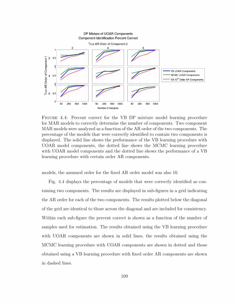
Figure 4.4: Percent correct for the VB DP mixture model learning procedurefor MAR models to correctly determine the number of components. Two componentMAR models were analyzed as a function of the AR order of the two components. Thepercentage of the models that were correctly identified to contain two components isdisplayed. The solid line shows the performance of the VB learning procedure withUOAR model components, the dotted line shows the MCMC learning procedurewith UOAR model components and the dotted line shows the performance of a VBlearning procedure with certain order AR components.

models, the assumed order for the fixed AR order model was also 10.

Fig. 4.4 displays the percentage of models that were correctly identified as con-

taining two components. The results are displayed in sub-figures in a grid indicating

the AR order for each of the two components. The results plotted below the diagonal

of the grid are identical to those across the diagonal and are included for consistency.

Within each sub-figure the percent correct is shown as a function of the number of

samples used for estimation. The results obtained using the VB learning procedure

with UOAR components are shown in solid lines, the results obtained using the

MCMC learning procedure with UOAR components are shown in dotted and those

obtained using a VB learning procedure with fixed order AR components are shown

in dashed lines.

109

From Fig. 4.4 it can be seen that VB approximate inference achieves similar

model order selection performance to the MCMC based learning procedure with the

performance MCMC inference achieving marginally higher performance in nearly all

conditions. This can be expected as MCMC sampling inference is known to provide a

better posterior approximation than the VB approximation [30]. The slight degrada-

tion in model order selection performance resulting from the VB approximation can

be justified in many applications where the other advantages of variational inference,

such as computational speed and quantifiable stopping criterion, are required.

The results in Fig. 4.4 also indicate that modeling uncertainty regarding the

AR order increases the ability of the DP learning procedure to correctly identify the

number of components within the model. Modeling this uncertainty has a greater

advantage over using an assumed value when the number of samples used for esti-

mation is smaller. As the number of samples used for estimation increases, the two

approaches achieve similar performance. Using an assumed, high AR order with a

small number of samples tends to over-fit to the data and as a result the number

components within the mixture is usually reduced to 1. Including uncertainty in the

AR order in these cases aids performance.

The results show that including uncertainty in the AR order enables the learning

procedure for the DP mixture model to correctly determine the number of compo-

nents within the MAR model more accurately than assuming a fixed AR order. This

provides a more robust method of automated model order selection within MAR

models. However, the accuracy of the estimated AR orders of the components of the

mixture model has not yet been addressed.

Fig. 4.5 provides results that address the ability of the DP mixture of UOAR

models to correctly determine the AR order of the components. The results are

reported in the same grid pattern as used in Fig. 4.4 but now the lines indicate

the number of correctly identified AR components as a function of the number of

110

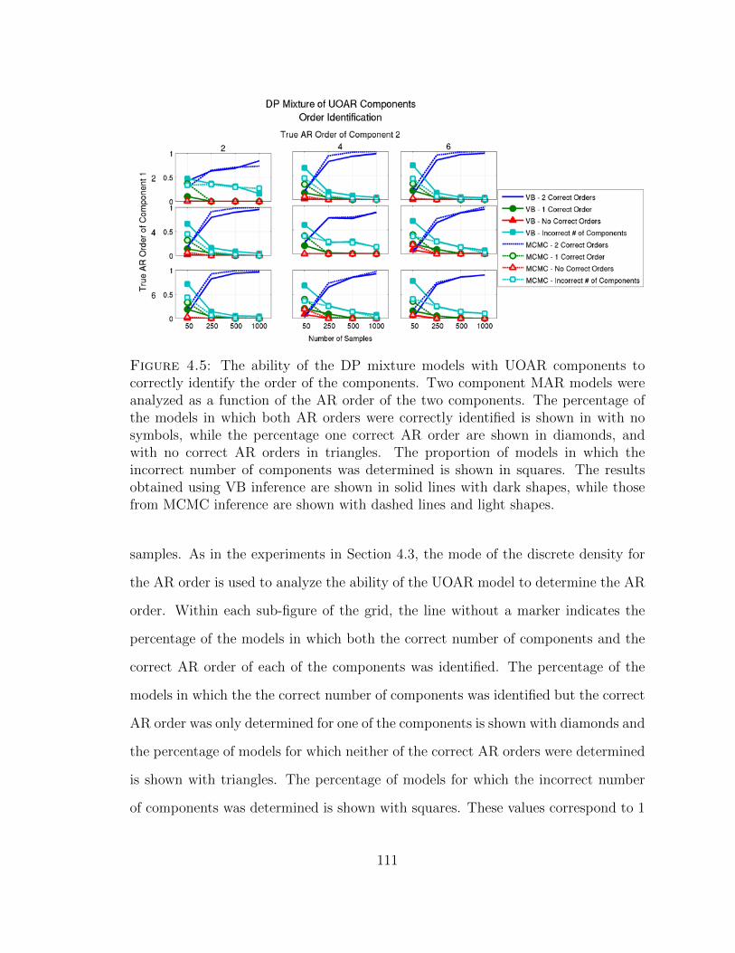
Figure 4.5: The ability of the DP mixture models with UOAR components tocorrectly identify the order of the components. Two component MAR models wereanalyzed as a function of the AR order of the two components. The percentage ofthe models in which both AR orders were correctly identified is shown in with nosymbols, while the percentage one correct AR order are shown in diamonds, andwith no correct AR orders in triangles. The proportion of models in which theincorrect number of components was determined is shown in squares. The resultsobtained using VB inference are shown in solid lines with dark shapes, while thosefrom MCMC inference are shown with dashed lines and light shapes.

samples. As in the experiments in Section 4.3, the mode of the discrete density for

the AR order is used to analyze the ability of the UOAR model to determine the AR

order. Within each sub-figure of the grid, the line without a marker indicates the

percentage of the models in which both the correct number of components and the

correct AR order of each of the components was identified. The percentage of the

models in which the the correct number of components was identified but the correct

AR order was only determined for one of the components is shown with diamonds and

the percentage of models for which neither of the correct AR orders were determined

is shown with triangles. The percentage of models for which the incorrect number

of components was determined is shown with squares. These values correspond to 1

111

minus the values plotted for the UOAR model in Fig. 4.4. For each of these lines

the results obtained using VB inference are shown with solid lines with dark shapes,

while those from MCMC inference are shown with dashed lines and light shapes.

These results indicate that when the DP mixture model learning procedure cor-

rectly determines the number of components both learning procedure are able to

correctly determines the AR orders of these components with a high degree of ac-

curacy provided sufficient data is available. Using both methds, the accuracy of the

estimated AR orders increases with the total number of observed samples. There

are no apparent trends in AR order estimation accuracy with regard to the true AR

order of the two components. Based on the results it appears as though the perfor-

mance of AR order determination is primarily determined by the number of samples

used for estimation and the ability of the DP mixture model learning procedure to

correctly determine the number of components.

Again, performance offered by MCMC inference is marginally superior to that

obtained with VB inference in almost all cases. This is most clearly visible by

comparing the lines without symbols, the proportion of trials in which the AR order

of both components was estimated correctly. In almost all cases the dashed line

appears above or equal to the solid line, indicating marginally superior performance.

As stated previously, the slight performance degradation may be acceptable when

more rapid model inference is required.

4.6 Classification of Acoustic Signals

The MAR model order selection experiment discussed above indicates that DP mix-

ture models with UOAR components can accurately determine the number of com-

ponents and the AR order of these components from synthetic data and that the

approximation provided by variational Bayesian inference is very close to that pro-

vided by MCMC inference. The efficacy of the VB learning procedure for the devel-

112

oped model and the importance of performing model order selection is now analyzed

within the context of an acoustic signal classification problem. Due to the similar-

ity between the posterior approximations obtained and the time that is required to

calculate the MCMC solution, only the VB approximation is used for the analysis

considered in this section. Furthermore, MCMC inference is inappropriate for the

acoustic sensing application of interest to this work.

The task under consideration is to classify four classes of acoustic signals that

are likely to be encountered by an acoustic surveillance system. Twenty five isolated

examples from four acoustic classes, glass breaking, doors slamming, pieces of wood

hitting together, and gunfire are examined and used to train and evaluate the per-

formance of each model. Each of the examples were sampled at 8kHz and energy

normalized. To ensure that the models are not trained and evaluated using the same

data a five fold cross-validation approach is utilized. Under this paradigm, the 25

examples from each class are separated such that a model is trained using 20 of the

examples and the remaining 5 are used for evaluation. This process is repeated until

each example has been evaluated.

Classification is performed by a assigning a sample to the class with the maximum

posterior probability. The posterior class probability when using the DP mixture of

UOAR components is determined by using the VB approximate likelihood of each

class. The VB approximate likelihood for class ω given example D is

q (D|c = ω) =T∑t=1

log∞∑i=1

exp(Sωt,i)

(4.44)

where the values Sωt,i are found by using (4.27) using the posterior hyperparameters

used for class ω. The posterior class probability is then determined using Bayes’

rule with a uniform prior over the classes. The posterior class probability for the

fixed order, fixed number of components MAR model is calculated similarly with the

exception that the likelihood of each class given an example is calculated using the

113

posterior predictive density instead of the VB approximation.

The classification performance achieved using the DP mixture of UOAR compo-

nents is compared to the performance achieved when the number of components and

the AR order of the components of a fixed order and fixed number of component

mixture model are varied. The necessity of model order selection for MAR mod-

els is indicated by changes in performance as a function of these parameters and

the utility of the DP mixture of UOAR components is indicated by achieving simi-

lar performance to the maximum performance obtained by varying the model order

parameters.

The performance of the MAR model is evaluated by allowing the AR order to

take values of 1, 2, 4, 6 or 10 and the number of components within the model

take values 1, 2, 5, 10 or 20. The components of the MAR are constrained to have

the same AR order. Although allowing the order of each the components to vary

may potentially yield better performance, the computational expense of testing each

possible combination when the number of components is large becomes very high.

The DP mixture of UOAR models is constructed to allow for a maximum number of

components, K, of 20 and a maximum AR order, M , of 10.

Fig. 4.6 shows the percent correct as a function of the assumed AR order and

number of components in MAR models as well as the percent correct achieved using

the DP mixture of UOAR components. The bar plots show the results for the

different model orders in MAR models grouped along the horizontal axis according to

the assumed AR order and shaded according to the number of assumed components

within the model. The results obtained using the DP mixture of UOAR components

is shown as the solid line at the 88.75%.

The DP mixture of UOAR components is able to achieve performance that is

equivalent to the best performance obtained by searching through model orders under

consideration for the fixed order, fixed number of components MAR model. This

114

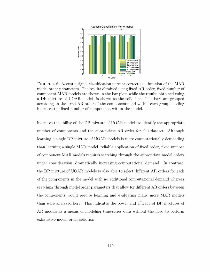
Figure 4.6: Acoustic signal classification percent correct as a function of the MARmodel order parameters. The results obtained using fixed AR order, fixed number ofcomponent MAR models are shown in the bar plots while the results obtained usinga DP mixture of UOAR models is shown as the solid line. The bars are groupedaccording to the fixed AR order of the components and within each group shadingindicates the fixed number of components within the model.

indicates the ability of the DP mixture of UOAR models to identify the appropriate

number of components and the appropriate AR order for this dataset. Although

learning a single DP mixture of UOAR models is more computationally demanding

than learning a single MAR model, reliable application of fixed order, fixed number

of component MAR models requires searching through the appropriate model orders

under consideration, dramatically increasing computational demand. In contrast,

the DP mixture of UOAR models is also able to select different AR orders for each

of the components in the model with no additional computational demand whereas

searching through model order parameters that allow for different AR orders between

the components would require learning and evaluating many more MAR models

than were analyzed here. This indicates the power and efficacy of DP mixtures of

AR models as a means of modeling time-series data without the need to perform

exhaustive model order selection.

115

4.7 Conclusions

This chapter has analyzed the UOAR model and investigated its use within DP mix-

ture models. The UOAR model provides a means of automated AR order estimation

by utilizing a discrete posterior density representing uncertainty about the AR or-

der. Incorporating UOAR components into DP mixture models creates an expressive

statistical model that automatically performs model order selection regarding both

the number of components within the mixture and the AR order of each component.

The ability of the UOAR model to correctly identify the AR order of synthetic

data was analyzed and compared to alternative techniques. This was done more

thoroughly than in previous investigations by analyzing randomly generated AR

models. Both UOAR modeling and the BIC are able to determines the correct

AR with a high degree of accuracy. The UOAR model, however, provides a full

posterior density for the AR model and therefore can be incorporate into larger

statistical models without the need to perform explicit model order selection for the

AR components.

The UOAR model was then incorporated into DP mixture models to create an

expressive model for time-series data. The VB learning procedure for DP mixtures

of UOAR models presented in this work offers a more computationally tractable

approach than the previously analyzed MCMC based learning procedure presented

in [20]. The learning procedure was then analyzed using randomly generated MAR

models and the accuracy of determining both the number of components within the

mixture as well the AR order of these components was investigated. The efficacy

of the DP mixture of UOAR components model was then illustrated through an

acoustic classification task. It was observed that using the DP mixture of UOAR

components model to perform automated model order selection yields performance

comparable to performing exhaustive model order selection for a range of different

116

model orders of fixed order models, with significantly less computational demand.

Although the DP mixture models analyzed in this chapter serve as a method

for determining the number of components in a model for acoustic signals, they do

not model the structure of the occurrence of these components. The underlying

model states that the component label at each time sample is drawn independently

of all other times. Therefore, when UOAR components are used to model acoustic

signals, only the frequency of occurrence of spectral and energy characteristics are

modeled. The next chapter analyzes the use of hidden Markov models (HMMs) with

UOAR components to model acoustic signals and to characterize the time structure

of the occurrence of the components, thus creating a better characterizing model for

acoustic signals.

117

5

Nonparametric Bayesian Acoustic SignalClassification

In the previous chapter, Bayesian inference was used to infer the parameters of statis-

tical models capable of performing automated model order selection. The variational

Bayes (VB) method was used to provide a rapid learning procedure that results in

a posterior density of the same functional form as the prior density, a desired cri-

terion that enables tractable and principled algorithmic adaption through the use

of recursive Bayesian estimation. Although the VB method provides a less accurate

approximation of the true posterior density than computational Markov chain Monte

Calro (MCMC) inference, the model order selection accuracy of the VB procedure

was nearly as accuracte the MCMC learning procedure when the number of data

samples is sufficient.

The Dirichlet process (DP) mixture of uncertain-order autoregressive (UOAR)

components analyzed in the last chapter served as a model that is capable of char-

acterizing acoustic signals by modeling the signal as a collection of spectral and

energy properties. However, because the model is a probabilistic mixture, only the

frequency of occurance of these components is modeled. A better characterizing and

118

more realistic model for acoustic signals can be created by not only modeling the

frequency of the occurrence of each of the components but also including a model

for sequential ordering of the components. A model of this type can be realized in a

tractable manner by considering a hidden Markov model (HMM) where each UOAR

model constitutes a component.

In this chapter a HMM with UOAR components is analyzed and used for time-

domain signal classification. As with mixture models, the use of HMMs requires

selection of the number of components within the model. The DP prior and model

construction once again provides the methodology to automatically select the number

of components, however, the use of the DP for HMMs is significantly different than

for mixture models. The resulting HMM formulation, with automatic selection of the

number of states making use of UOAR sources provides a completely nonparametric

model for not only acoustic signals, but many other types of time series signals.

To analyze the efficacy of the proposed model, the application of the proposed

nonparametric model for the acoustic sensing task considered in this work is first

analyzed. It is demonstrated that the statistical model is capable of characterizing

the acoustic surveillance signals under consideration and that it enables accurate

classification and offers performance improvements over alternative feature based

classification schemes. Furthermore, since the model is generative and operates in the

time-domain, the model is also capable of generating synthetic acoustic signals using

the inferred model parameters, an interesting corollary of the proposed approach. In

addition to being able to classify acoustic surveillance signals of interest such as glass

breaking and muzzle blasts, the statistical model is also capable of discriminating

between very similar sounds of interest. This is illustrated by utilizing the model to

distinguish between different types guns through recordings of muzzle blasts. The

ability to discriminate between such similar sounds with a high degree of accuracy

motivates the hierarchical model structure for a collection of time-series analyzed in

119

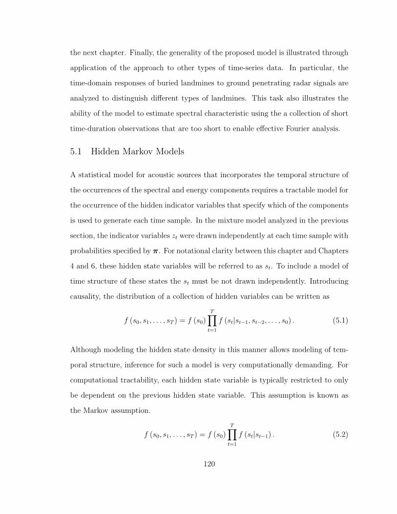
the next chapter. Finally, the generality of the proposed model is illustrated through

application of the approach to other types of time-series data. In particular, the

time-domain responses of buried landmines to ground penetrating radar signals are

analyzed to distinguish different types of landmines. This task also illustrates the

ability of the model to estimate spectral characteristic using the a collection of short

time-duration observations that are too short to enable effective Fourier analysis.

5.1 Hidden Markov Models

A statistical model for acoustic sources that incorporates the temporal structure of

the occurrences of the spectral and energy components requires a tractable model for

the occurrence of the hidden indicator variables that specify which of the components

is used to generate each time sample. In the mixture model analyzed in the previous

section, the indicator variables zt were drawn independently at each time sample with

probabilities specified by π. For notational clarity between this chapter and Chapters

4 and 6, these hidden state variables will be referred to as st. To include a model of

time structure of these states the st must be not drawn independently. Introducing

causality, the distribution of a collection of hidden variables can be written as

f (s0, s1, . . . , sT ) = f (s0)T∏t=1

f (st|st−1, st−2, . . . , s0) . (5.1)

Although modeling the hidden state density in this manner allows modeling of tem-

poral structure, inference for such a model is very computationally demanding. For

computational tractability, each hidden state variable is typically restricted to only

be dependent on the previous hidden state variable. This assumption is known as

the Markov assumption.

f (s0, s1, . . . , sT ) = f (s0)T∏t=1

f (st|st−1) . (5.2)

120

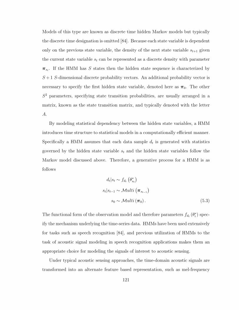
Models of this type are known as discrete time hidden Markov models but typically

the discrete time designation is omitted [84]. Because each state variable is dependent

only on the previous state variable, the density of the next state variable st+1 given

the current state variable st can be represented as a discrete density with parameter

πst . If the HMM has S states then the hidden state sequence is characterized by

S+ 1 S-dimensional discrete probability vectors. An additional probability vector is

necessary to specify the first hidden state variable, denoted here as π0. The other

S2 parameters, specifying state transition probabilities, are usually arranged in a

matrix, known as the state transition matrix, and typically denoted with the letter

A.

By modeling statistical dependency between the hidden state variables, a HMM

introduces time structure to statistical models in a computationally efficient manner.

Specifically a HMM assumes that each data sample dt is generated with statistics

governed by the hidden state variable st and the hidden state variables follow the

Markov model discussed above. Therefore, a generative process for a HMM is as

follows

dt|st ∼ fdt(θ∗st)

st|st−1 ∼Multi(πst−1

)s0 ∼Multi (π0) . (5.3)

The functional form of the observation model and therefore parameters fdt (θ∗i ) spec-

ify the mechanism underlying the time-series data. HMMs have been used extensively

for tasks such as speech recognition [84], and previous utilization of HMMs to the

task of acoustic signal modeling in speech recognition applications makes them an

appropriate choice for modeling the signals of interest to acoustic sensing.

Under typical acoustic sensing approaches, the time-domain acoustic signals are

transformed into an alternate feature based representation, such as mel-frequency

121

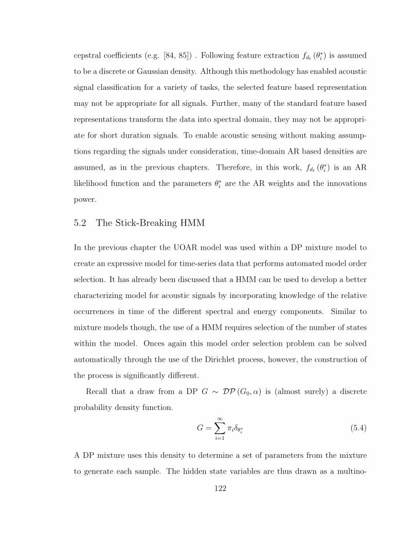
cepstral coefficients (e.g. [84, 85]) . Following feature extraction fdt (θ∗i ) is assumed

to be a discrete or Gaussian density. Although this methodology has enabled acoustic

signal classification for a variety of tasks, the selected feature based representation

may not be appropriate for all signals. Further, many of the standard feature based

representations transform the data into spectral domain, they may not be appropri-

ate for short duration signals. To enable acoustic sensing without making assump-

tions regarding the signals under consideration, time-domain AR based densities are

assumed, as in the previous chapters. Therefore, in this work, fdt (θ∗i ) is an AR

likelihood function and the parameters θ∗i are the AR weights and the innovations

power.

5.2 The Stick-Breaking HMM

In the previous chapter the UOAR model was used within a DP mixture model to

create an expressive model for time-series data that performs automated model order

selection. It has already been discussed that a HMM can be used to develop a better

characterizing model for acoustic signals by incorporating knowledge of the relative

occurrences in time of the different spectral and energy components. Similar to

mixture models though, the use of a HMM requires selection of the number of states

within the model. Onces again this model order selection problem can be solved

automatically through the use of the Dirichlet process, however, the construction of

the process is significantly different.

Recall that a draw from a DP G ∼ DP (G0, α) is (almost surely) a discrete

probability density function.

G =∞∑i=1

πiδθ∗i (5.4)

A DP mixture uses this density to determine a set of parameters from the mixture

to generate each sample. The hidden state variables are thus drawn as a multino-

122

mial density with infinite parameter vector π. Also recall that the stick-breaking

representation [22] can be used to transform the estimation of the infinite proba-

bility vector π to estimation of an infinite collection of variables between 0 and 1,

ρ. Transformation of the probability vector to ρ enables truncation of the number

of components at an arbitrary high level which maintains a good approximation to

the DP [82]. The stick breaking construction enables the use of VB inference for

DP mixture models and thus enabling a learning procedure for mixture models with

automated number of components selection.

Using a DP mixture model, a mixture with an infinite number of components

can be realized. Recall from the discussion of HMMs above that, given the current

hidden state st, the next observation dt follows a mixture model with component

probabilities given by πst and component parameters θ∗i for 1 ≤ i ≤ S. To consider

a DP based HMM it would appear natural to consider each state to be governed by

a DP mixture model and therefore state j is determined by

Gj ∼ DP (G0, α)

Gj =∞∑i=1

πj,iδθ∗j,i . (5.5)

However, under this construction each Gj is independently drawn from the under-

lying DP and therefore, each θ∗j,i is an independent draw from G0. Since G0 is a

continuous density (determined by the observation model under consideration), each

θ∗j,i is unique with probability 1 and therefore, the resulting model would is not a

HMM.

Proper use of the DP for HMM construction was first analyzed in [86] by using

the hierarchical Dirichlet process (HDP) [24]. The infinite HMM (iHMM) is formed

by considering a collection of DP mixtures that share a common based density that

is itself a draw from a DP. The DP draw governing state j is now drawn from a

123

DP with base density H. The base density H is also drawn from a DP with a base

density G0 determined by the observation model under consideration.

H ∼ DP (G0, α)

Gj ∼ DP (H,α)

Gj =∞∑i=1

πj,iδθ∗i . (5.6)

The inclusion of the intermediary DP draw H ensures that the Gjs share the θ∗i s.

Because H is a draw from a DP it is a discrete base density and thus it is possible

to independently draw identical θ∗i . The hierarchical nature of the iHMM creates a

statistical model that, when parameter inference is performed, inherently estimates

the appropriate model order. However, due to the hierarchical nature the relationship

between G0 and each Gj is not conjugate. Therefore, it is not possible to perform

VB inference and MCMC based inference must be utilized.

In [23], an alternative formulation to the iHMM is developed. The stick-breaking

HMM (SBHMM) utilizes the stick-breaking construction for the infinite probabil-

ity vectors πj within each state and assumes that each state shares the same θ∗i .

Therefore, the model is simply

θ∗i ∼ G0

Gj =∞∑i=1

πj,iδθ∗i . (5.7)

Although superficially identical to the iHMM, the two are mathematically distinct.

The SBHMM has no relation to DP beyond the stick-breaking construction but

because it is not dependent on the HDP it is possible to perform VB parameter

inference. To draw an analogy to the standard HMM, a SBHMM has a state tran-

sition matrix in which each row πj is represented by a stick-breaking construction

with parameters ρj. If the stick-breaking proportion ρi,j is modeled using a beta

124

density β (γi,j,1, γi,j,2) the generative process of a SBHMM can be written as follows.

dt|st ∼ fdt(θ∗st)

st|st−1 ∼Multi(πst−1

)s0 ∼Multi (π0)

πi = SB (ρi)

ρi,j ∼ β (γi,j,1, γi,j,2) (5.8)

5.3 A Nonparametric Bayesian Time Series Model

Utilizing UOAR models within a SBHMM creates a model for time-series data that

provides automated model order selection in both the number of unique spectral and

energy components and the spectral complexity of each of the components, while

simultaneously modeling the time structure of the occurrence of the components.

This model is similar in form to that presented in [26] in that a HMM with AR

sources is utilized. There are two primary differences between this work and that of

[26]. First, this work utilizes the UOAR model structure, analyzed in the previous

chapter, to provide automatic order selection within each state of the HMM. Second

this work utilizes the SBHMM model structure as apposed to the HDP based iHMM

thus making VB inference possible. By utilizing the iHMM, only MCMC inference

is possible as conducted in [26]. Utilization of the SBHMM and the UOAR model

structure allows for VB inference for statistical model appropriate for the acoustic

sensing tasks of focus to this work.

To incorporate an UOAR model into the SBHMM, the density function governing

each state is assumed to be an UOAR model and therefore the parameters for each

state θ∗i are the AR order, AR weights and the innovations power. Recall from the

125

previous chapter that the UOAR model has the following generative process

dt ∼ Ndt (a′ψt, r)

a, r|m ∼ N iWa,r (vm,Vm)

m ∼ Discrete (µ, [1, . . . ,M ]) . (5.9)

Also recall that the conjugate prior for this model is the discrete-Normal-inverse-

Wishart density which is parameterized by M sets of Normal-inverse-Wishart param-

eters, νi, and Vi and the M dimensional discrete probability vector µ. Combining

the parameters of the SBHMM and the UOAR model for each state creates a prior

structure as follows

f (·) = f(stT1

) S∏i=1

βρ0,i

(γ0

0,i,1, γ00,i,2

)

·S∏i=1

S∏j=1

βρi,j(γ0i,j,1, γ

0i,j,2

)

·S∏i=1

M∑l=1

µ0i,lN iWai,ll,ri,l

(ν0i,l,V

0i,l

). (5.10)

Here it has been assumed that each UOAR model has a maximum order of M and

the HMM has a maximum of S states. The first two terms of this prior density are

the prior structure for the hidden state sequence and the SB parameters for the initial

state variable probability vector. The third term comprises the S2 SB parameters

for the state transition matrix. The final term is the UOAR model prior for each of

the S states.

5.3.1 Model Inference

To perform Bayesian parameter inference for the above model, the posterior density

must be determined given observed data, D. As the required inference is intractable,

the VB method is again employed. To apply the VB method to this model, the

126

first step is to make appropriate independence assumptions for the posterior density.

The functional form of the selected prior structure, as shown in (5.10), is conjugate

to each of the necessary components in the model. Therefore, it is computationally

convenient to assume that the approximate posterior density has the same functional

form with updated parameters.

q (·) = q(stT1

) S∏i=1

βρ0,i (γ0,i,1, γ0,i,2)

·S∏i=1

S∏j=1

βρi,j (γi,j,1, γi,j,2)

·S∏i=1

M∑l=1

µi,lN iGai,l,ri,l (νi,l,Vi,l)

(5.11)

For the SBHMM with UOAR sources, the VB method results in an algorithm

that is similar in form to that of expectation maximization for a standard HMM

[84]. Following initialization (discussed in the next section), the first step of each

iteration is to redetermine the posterior approximate of the hidden state variables

q(stT1

). Recall that the VB method iteratively updates the posterior density for

each parameter to be proportional to the expected value of the likelihood function

with the expected value taken with respect to the current estimate of the posterior

density for all other parameters.

log q (θi) ∝ Eq(θ−i)log f (D, θ) (5.12)

Applying (5.12) to the hidden state sequence with respect to all other parameters

yields

log q(stT1

)∝ Elog π0,s1+

T∑t=2

Elog πst−1,st+T∑t=1

Elog f (dt, ast , rst ,mst).

(5.13)

In (5.13) and in the remainder of this section, the expected values are taken with

respect to the current approximate distributions for all unknown parameters. It

127

should be noted that (5.13) is similar to the hidden state update equation for a

standard HMM with the fundamental difference that each parameter is replaced

by its expected value. Therefore, (5.13) can be determined by using the forward-

backwards algorithm as in a standard HMM by replacing the necessary quantities

with their expected values.

For a standard HMM, the forwards-backwards algorithm determines the proba-

bility of each hidden state for each observation by considering the probability of each

path from the forward direction and the probability of each state from the backwards

direction. The joint probability of the entire dataset and a hidden state variable, st,

can be partitioned into the “forwards” variable, α, and the “backwards” variable, β.

Let Θ represent all of the parameters of the HMM. Using this notation, the likelihood

of the entire dataset and a single hidden state variable st is

f (DT , st = i|Θ) = αt (i) βt (i) . (5.14)

The forwards and backwards variables are defined as

αt (i) = f (d1, . . . , dt, st = i|DT , θN) (5.15)

βt (i) = f (dt+1, . . . , dT |st = i,DT , θN) . (5.16)

The probability of each hidden state at each time is then proportional to the product

of the forward and backwards variables

f (st = i|Θ) ∝ αt (i) βt (i) . (5.17)

Determining the values of αt (i) and βt (i) at each time must be done recursively.

The forward variable, α, begins with the definition

α1 (i) = π0,if (d1|st = i, θ∗i ) (5.18)

which is defined in terms of the initial state probability. The forward variable at

128

each future time is determine recursively as follows.

αt (i) =

[S∑j=1

πijαt−1 (j)

]f (dt|Dt−1, θ

∗i ) (5.19)

The backwards variable begins with the definition that βT (i) = 1 and each previous

β is also determined recursively.

βt (i) =

[S∑j=1

πijβt+1 (j)

]f (dt|Dt−1, θ

∗i ) (5.20)

By calculating both the forward and backwards variables for each observation, the

probability density of the hidden state variable at each time can be determined. In

addition to this quantity, the probability of transitioning from state i to state j at

time t can be determined from the forwards and backwards variables

ξt (i, j) ∝ αt (i) πijf(dt+1|st+1 = j,Dt, θ

∗j

)βt+1 (j) . (5.21)

This quantity is necessary to update the state transition matrix in a fixed order HMM

and the stick-breaking proportion parameters in a SBHMM. To perform expectation

maximization for a the parameters of an HMM with a fixed number of states, the

forward-backwards algorithm is used to determine a probability density for the hid-

den state sequence and this value is subsequently used to re-estimate each of the

parameters of the HMM. A very similar algorithm results from the VB method.

To evaluate (5.13) and determine the posterior density of the hidden state se-

quence under the VB method, the forward-backwards algorithm can be utilized by

replacing the necessary parameters in (5.19 - 5.21) with the appropriate expected

129

values.

αVBt (i) =

[S∑j=1

expElog πi,j

αVBt−1 (j)

]exp

Elog f (dt, ai, ri,mi)

(5.22)

βVBt (i) =

[S∑j=1

expElog πi,j

βVBt+1 (j)

]exp

Elog f (dt, ai, ri,mi)

(5.23)

ξVBt (i, j) ∝ αVB

t (i) expElog πi,j

exp

Elog f (dt+1, |aj, rj,mj)

βVBt+1 (j) .

(5.24)

Therefore, to employ the VB equivalent of the forward-backwards algorithm and

reestimate the posterior density for the hidden state sequence, two quantities are

required, Elog πi,j and Elog f (dt, ast , rst ,mst).

The first of these required quantities, the expected value for the log of a discrete

probability vector utilizing a stick-breaking prior, is determined by moments of the

beta density which model the stick-breaking proportions.

Elog ρi,j = ψ (γi,j,1)− ψ (γi,j,1 + γi,j,2)

Elog (1− ρi,j) = ψ (γi,j,2)− ψ (γi,j,1 + γi,j,2)

Elog πi,j = Elog ρi,j+

j−1∑k=1

Elog (1− ρi,k) (5.25)

The second required quantity, the expected value of the log of the observation model

for the UOAR model, was determined in the previous chapter. This is realized by

first calculating the expected value with respect to the AR order

Elog f (dt|ψt,m, a, r) =M∑i=1

q (m = i)Eq(a,r|m=i)log f(dt|ψi

t, ai, r) (5.26)

and then determining the expected value over the Normal-inverse-Wishart with a

130

fixed order

Eq(a,r|m=l)log f(dt|ψl

t, al, r) = −1

2log π − 1

2Ψ

(ν − l − 2

2

)− 1

2log λ

− 1

2ψ′tV

−1aaψt −

(ν − l − 2)

2λ(dt − a′ψt)

2. (5.27)

Using (5.25) and (5.26), (5.13) can be determined via the forward-backwards algo-

rithm yielding the posterior probability of each sample belonging to each state, q (st),

and the probability of transitioning from state i to state j for each sample, ξVBt (i, j).

From ξVBt (i, j) the the expected number of transitions from state i to state j, ni,j

can be determined.

ni,j =T∑t=1

ξVBt (i, j) (5.28)

This quantity can be used to re-estimate the hyperparameters for the beta density,

modeling knowledge of each stick breaking proportion.

γi,j,1 = γ0i,j,1 + ni,j (5.29)

γi,j,2 = γ0i,j,2 +

S∑k=j+1

ni,k (5.30)

The initial state probability vector, determined from γ0,j,1 and γ0,j,2 can be found

by replacing n0,j with q (s0 = j). The values of γ0i,j,1 and γ0

i,j,1 are prior parameters

discussed below. Applying these update equations for each i and j determines a

new estimate of the parameters of the beta density modeling knowledge in each

stick-breaking proportion. These stick-breaking proportions ultimately specify our

knowledge of the transition matrix and initial state probability vector, two of our

primary parameters of interest.

Finally, the hyperparameters for the discrete-Normal-inverse-Wishart density gov-

erning the UOAR model within each state must be redetermined. This requires up-

dating the M sets of Normal-inverse-Wishart parameters, the matrix Vl and scalar

131

νl for l ∈ 1, . . . ,M], and the discrete probability vector for the AR order. Us-

ing the probability of each hidden state for each sample, q (st), obtained from VB

forwards-backwards, the Normal-inverse-Wishart parameters in state i for AR order

l can by evaluating

q (ai, ri|mi = l) =T∏t=1

(f (dt|ψt, ai, ri,mi = l))q(st=i) f(ai, ri|V0

l , ν0l

)(5.31)

This is equivalent to (4.35) replacing q (zt = i) with q (st = i). Therefore, the param-

eters are updated as follows

Vi,l = V0l +

T∑t=1

q (st = i)φlt(φlt)′

(5.32)

νi,l = ν0l +

T∑t=1

q (st = i) . (5.33)

The values of V0l and ν0

l are prior parameters that are discussed below. Following the

calculation of the Normal-inverse-Wishart parameters for each state and AR order,

the discrete density over the AR order can be determined for each state using the

standard UOAR model order estimation equation (4.15).

µi,l ∝ µ0l

Z (Vi,l, νi,l)

Z (V0l , ν

0l ). (5.34)

Using (5.32)-(5.34) the parameters governing the probability density function for

the UOAR model in each state can be re-estimated. Following calculation of these

quantities the VB forward-backwards algorithm can be re-applied to re-calculate

(5.25) which is then used to update the stick-breaking proportions and the state

density variables in a manner very similar to the standard expectation maximization

approach to HMM modeling.

After each iteration of the algorithm, the negative free energy F (·) can be calcu-

lated to monitor convergence. Recall that the negative free energy can be calculated

132

Initialize parameters using the method discussed in Section 5.3.3F = 0;repeatFold ← FUpdate q (st = i) ∀ i and ∀ t using VB Forward-backwards (5.22-5.26)Update q (ρi,j) ∀ i and ∀ j and q (ai, ri,mi) ∀ i using (5.30-5.34)Calculated F using (5.36)

until F − Fold < ε

Algorithm 2: VB Learning Procedure for a UOAR SBHMM

as

F (q (θ)) = Eq(θ)log f (D|θ) −KL (q (θ) ||f (θ)) . (5.35)

For the UOAR SBHMM this can be calculated as

F =T∑t=1

S∑i=1

Elog f (st = i)+ Elog f (dt|st = i, θ∗1, . . . , θ

∗S)

−S∑i=1

KL (q (ai, ri,mi) ||p (ai, ri,mi))−S∑i=0

S∑j=1

KL (q (ρi,j) ||p (ρi,j)) (5.36)

where p (·) represents the distribution of the quantity using the prior parameters.

The first term can be determined from q (st) and (5.26) while the last two terms are

Kullback-Leibler divergence terms between discrete-Normal-inverse-Wishart densi-

ties and beta densities, respectively. These values are discussed in the Appendix

A.

VB learning for a the UOAR SBHMM is summarized in Algorithm 2. The re-

sulting algorithm is very similar to the standard EM approach for maximum likeli-

hood estimation of HMM parameters with each step making use of the VB forward-

backwards algorithm and updating hyperparameters instead of reestimating the pa-

rameters.

Although this model has been learned assuming that there are S hidden states

many of these states will not be used due to the stick-breaking prior for each row

of the state transition matrix. After optimization, many states will have no samples

133

with a high probability of membership. Therefore, for future purposes these states

can be removed from the model. It is thus advantageous to select S as high as

computationally allowable, and the optimization procedure will use a few states as

is necessary.

5.3.2 Prior Parameters

The prior parameters were selected to have minimal effect on the resulting learned

parameters. The parameters of V0l and ν0

l were selected to correspond to AR weights

with zero mean and a diagonal covariance matrix with variance 1000 and an inno-

vations power with a mean of 1 and a variance of 1000 as in the previous chapter.

The values of γ0i,j,1 and γ0

i,j,2, control the preference for sparsity in the number of de-

termined states within the HMM. These parameters were set to 2 and 1 respectively

and not tuned relative to data.

5.3.3 Implementation

Like most optimization procedures the VB method requires a sufficient initialization

of the parameters to avoid a local minimum. The same initialization scheme as the

previous chapter is employed. First, maximum likelihood estimates of AR model

parameters are calculated for segments of the input sequence. These sets of AR

parameters are then clustered into S groups using k-means and from these clusterings

an initial state is assigned to each time sample. These state assignments are then

used to initialize q (st) and the algorithm begins by calculating the stick-breaking

proportions.

5.3.4 Example

The developed VB learning procedure for the UOAR SBHMM is now illustrated

on synthetic data. A sequence of data was generated from a HMM with two states.

Within each state the probability of a self state transition is 0.995 and the probability

134

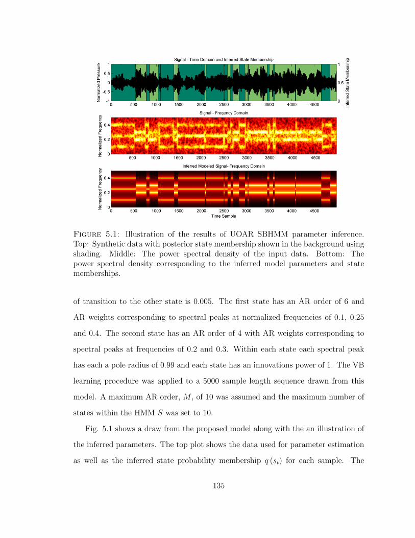
Figure 5.1: Illustration of the results of UOAR SBHMM parameter inference.Top: Synthetic data with posterior state membership shown in the background usingshading. Middle: The power spectral density of the input data. Bottom: Thepower spectral density corresponding to the inferred model parameters and statememberships.

of transition to the other state is 0.005. The first state has an AR order of 6 and

AR weights corresponding to spectral peaks at normalized frequencies of 0.1, 0.25

and 0.4. The second state has an AR order of 4 with AR weights corresponding to

spectral peaks at frequencies of 0.2 and 0.3. Within each state each spectral peak

has each a pole radius of 0.99 and each state has an innovations power of 1. The VB

learning procedure was applied to a 5000 sample length sequence drawn from this

model. A maximum AR order, M , of 10 was assumed and the maximum number of

states within the HMM S was set to 10.

Fig. 5.1 shows a draw from the proposed model along with the an illustration of

the inferred parameters. The top plot shows the data used for parameter estimation

as well as the inferred state probability membership q (st) for each sample. The

135

state probability membership is shown in the background with shading and it can be

seen that only two states are used. Therefore, the model order selection properties

of the stick-breaking prior have successfully determined that there are two states

in the model. The remaining 8 states have no samples assigned to them and thus

the statistics governing the density of the data within the states are equal to the

prior. The middle plot of Fig. 5.1 shows the short-time Fourier transform of the

sequence while the bottom plot shows a representation of the modeled short-time

Fourier transform. The mean of the density for AR weights with highest probability

within each state is combined with the inferred state probability membership to

show the modeled spectrogram of the input data. It can be seen that this modeled

spectrogram closely match that of the true data and that the number of and locations

of the spectral peaks within each state as well as the state transitions closely matche

the underlying model.

5.4 Applications of the UOAR SBHMM

The UOAR SBHMM is now used to model a variety of acoustic signals to demon-

strate the efficacy of the model for real-world signals. The applications are focused

on the classification of time-series data as this is the primary intended use of the

UOAR SBHMM within the acoustic sensing system of interest to this work. First,

the UOAR SBHMM parameters that are estimated from a collection of muzzle blasts

are examined. The results demonstrate the automated model order selection prop-

erties of the model and the ability to characterize the spectral content of real-world

signals. Following this, the UOAR SBHMM parameters inferred from a collection

of acoustic signals are used to generate synthetic signals. Comparison of the spec-

trograms of an example real-signal and a random draw from the UOAR SBHMM

with inferred parameters are provides further insight into the signal characteristics

that are quantified by the model parameters. Finally, the UOAR SBHMM is used

136

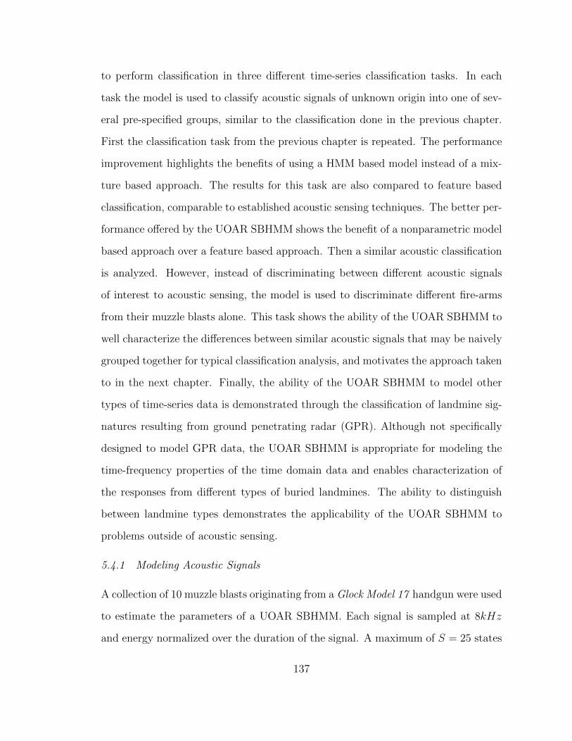
to perform classification in three different time-series classification tasks. In each

task the model is used to classify acoustic signals of unknown origin into one of sev-

eral pre-specified groups, similar to the classification done in the previous chapter.

First the classification task from the previous chapter is repeated. The performance

improvement highlights the benefits of using a HMM based model instead of a mix-

ture based approach. The results for this task are also compared to feature based

classification, comparable to established acoustic sensing techniques. The better per-

formance offered by the UOAR SBHMM shows the benefit of a nonparametric model

based approach over a feature based approach. Then a similar acoustic classification

is analyzed. However, instead of discriminating between different acoustic signals

of interest to acoustic sensing, the model is used to discriminate different fire-arms

from their muzzle blasts alone. This task shows the ability of the UOAR SBHMM to

well characterize the differences between similar acoustic signals that may be naively

grouped together for typical classification analysis, and motivates the approach taken

to in the next chapter. Finally, the ability of the UOAR SBHMM to model other

types of time-series data is demonstrated through the classification of landmine sig-

natures resulting from ground penetrating radar (GPR). Although not specifically

designed to model GPR data, the UOAR SBHMM is appropriate for modeling the

time-frequency properties of the time domain data and enables characterization of

the responses from different types of buried landmines. The ability to distinguish

between landmine types demonstrates the applicability of the UOAR SBHMM to

problems outside of acoustic sensing.

5.4.1 Modeling Acoustic Signals

A collection of 10 muzzle blasts originating from a Glock Model 17 handgun were used

to estimate the parameters of a UOAR SBHMM. Each signal is sampled at 8kHz

and energy normalized over the duration of the signal. A maximum of S = 25 states

137

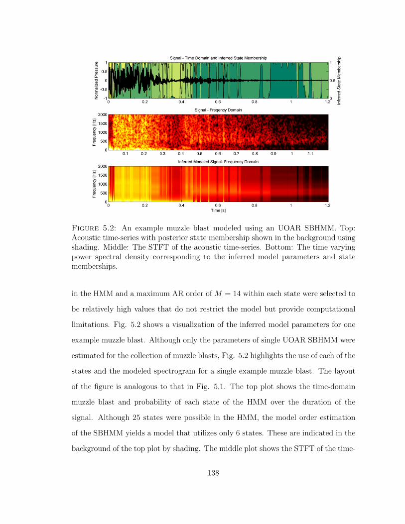
Figure 5.2: An example muzzle blast modeled using an UOAR SBHMM. Top:Acoustic time-series with posterior state membership shown in the background usingshading. Middle: The STFT of the acoustic time-series. Bottom: The time varyingpower spectral density corresponding to the inferred model parameters and statememberships.

in the HMM and a maximum AR order of M = 14 within each state were selected to

be relatively high values that do not restrict the model but provide computational

limitations. Fig. 5.2 shows a visualization of the inferred model parameters for one

example muzzle blast. Although only the parameters of single UOAR SBHMM were

estimated for the collection of muzzle blasts, Fig. 5.2 highlights the use of each of the

states and the modeled spectrogram for a single example muzzle blast. The layout

of the figure is analogous to that in Fig. 5.1. The top plot shows the time-domain

muzzle blast and probability of each state of the HMM over the duration of the

signal. Although 25 states were possible in the HMM, the model order estimation

of the SBHMM yields a model that utilizes only 6 states. These are indicated in the

background of the top plot by shading. The middle plot shows the STFT of the time-

138

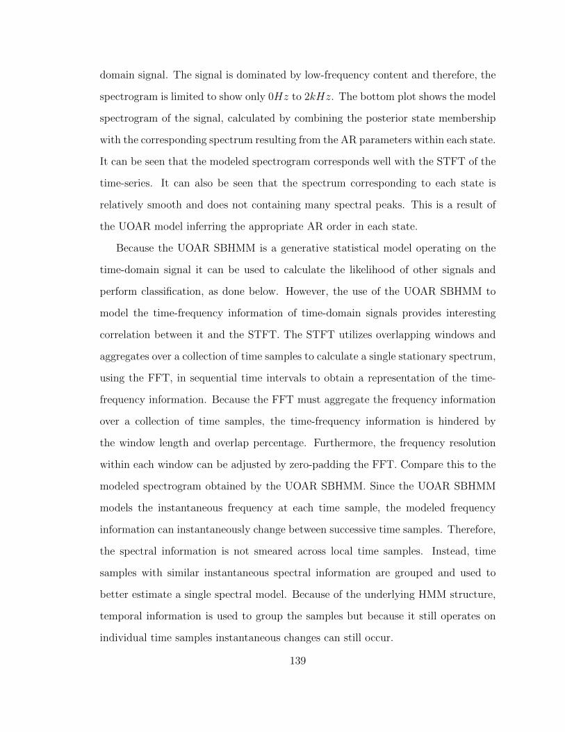
domain signal. The signal is dominated by low-frequency content and therefore, the

spectrogram is limited to show only 0Hz to 2kHz. The bottom plot shows the model

spectrogram of the signal, calculated by combining the posterior state membership

with the corresponding spectrum resulting from the AR parameters within each state.

It can be seen that the modeled spectrogram corresponds well with the STFT of the

time-series. It can also be seen that the spectrum corresponding to each state is

relatively smooth and does not containing many spectral peaks. This is a result of

the UOAR model inferring the appropriate AR order in each state.

Because the UOAR SBHMM is a generative statistical model operating on the

time-domain signal it can be used to calculate the likelihood of other signals and

perform classification, as done below. However, the use of the UOAR SBHMM to

model the time-frequency information of time-domain signals provides interesting

correlation between it and the STFT. The STFT utilizes overlapping windows and

aggregates over a collection of time samples to calculate a single stationary spectrum,

using the FFT, in sequential time intervals to obtain a representation of the time-

frequency information. Because the FFT must aggregate the frequency information

over a collection of time samples, the time-frequency information is hindered by

the window length and overlap percentage. Furthermore, the frequency resolution

within each window can be adjusted by zero-padding the FFT. Compare this to the

modeled spectrogram obtained by the UOAR SBHMM. Since the UOAR SBHMM

models the instantaneous frequency at each time sample, the modeled frequency

information can instantaneously change between successive time samples. Therefore,

the spectral information is not smeared across local time samples. Instead, time

samples with similar instantaneous spectral information are grouped and used to

better estimate a single spectral model. Because of the underlying HMM structure,

temporal information is used to group the samples but because it still operates on

individual time samples instantaneous changes can still occur.

139

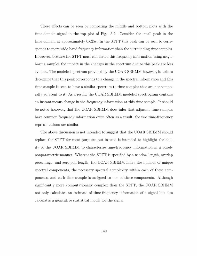
These effects can be seen by comparing the middle and bottom plots with the

time-domain signal in the top plot of Fig. 5.2. Consider the small peak in the

time domain at approximately 0.625s. In the STFT this peak can be seen to corre-

sponds to more wide-band frequency information than the surrounding time samples.

Howerver, because the STFT must calculated this frequency information using neigh-

boring samples the impact in the changes in the spectrum due to this peak are less

evident. The modeled spectrum provided by the UOAR SBHMM however, is able to

determine that this peak corresponds to a change in the spectral information and this

time sample is seen to have a similar spectrum to time samples that are not tempo-

rally adjacent to it. As a result, the UOAR SBHMM modeled spectrogram contains

an instantaneous change in the frequency information at this time sample. It should

be noted however, that the UOAR SBHMM does infer that adjacent time samples

have common frequency information quite often as a result, the two time-frequency

representations are similar.

The above discussion is not intended to suggest that the UOAR SBHMM should

replace the STFT for most purposes but instead is intended to highlight the abil-

ity of the UOAR SBHMM to characterize time-frequency information in a purely

nonparametric manner. Whereas the STFT is specified by a window length, overlap

percentage, and zero-pad length, the UOAR SBHMM infers the number of unique

spectral components, the necessary spectral complexity within each of these com-

ponents, and each time-sample is assigned to one of these components. Although

significantly more computationally complex than the STFT, the UOAR SBHMM

not only calculates an estimate of time-frequency information of a signal but also

calculates a generative statistical model for the signal.

140

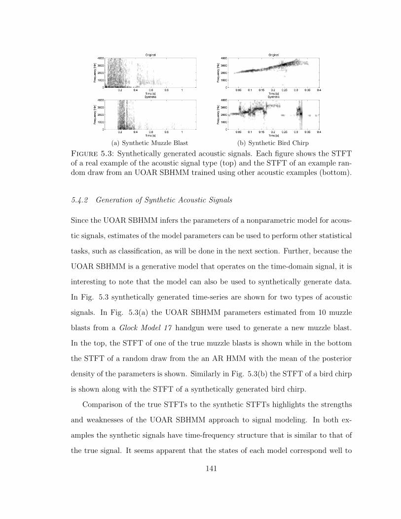
(a) Synthetic Muzzle Blast (b) Synthetic Bird Chirp

Figure 5.3: Synthetically generated acoustic signals. Each figure shows the STFTof a real example of the acoustic signal type (top) and the STFT of an example ran-dom draw from an UOAR SBHMM trained using other acoustic examples (bottom).

5.4.2 Generation of Synthetic Acoustic Signals

Since the UOAR SBHMM infers the parameters of a nonparametric model for acous-

tic signals, estimates of the model parameters can be used to perform other statistical

tasks, such as classification, as will be done in the next section. Further, because the

UOAR SBHMM is a generative model that operates on the time-domain signal, it is

interesting to note that the model can also be used to synthetically generate data.

In Fig. 5.3 synthetically generated time-series are shown for two types of acoustic

signals. In Fig. 5.3(a) the UOAR SBHMM parameters estimated from 10 muzzle

blasts from a Glock Model 17 handgun were used to generate a new muzzle blast.

In the top, the STFT of one of the true muzzle blasts is shown while in the bottom

the STFT of a random draw from the an AR HMM with the mean of the posterior

density of the parameters is shown. Similarly in Fig. 5.3(b) the STFT of a bird chirp

is shown along with the STFT of a synthetically generated bird chirp.

Comparison of the true STFTs to the synthetic STFTs highlights the strengths

and weaknesses of the UOAR SBHMM approach to signal modeling. In both ex-

amples the synthetic signals have time-frequency structure that is similar to that of

the true signal. It seems apparent that the states of each model correspond well to

141

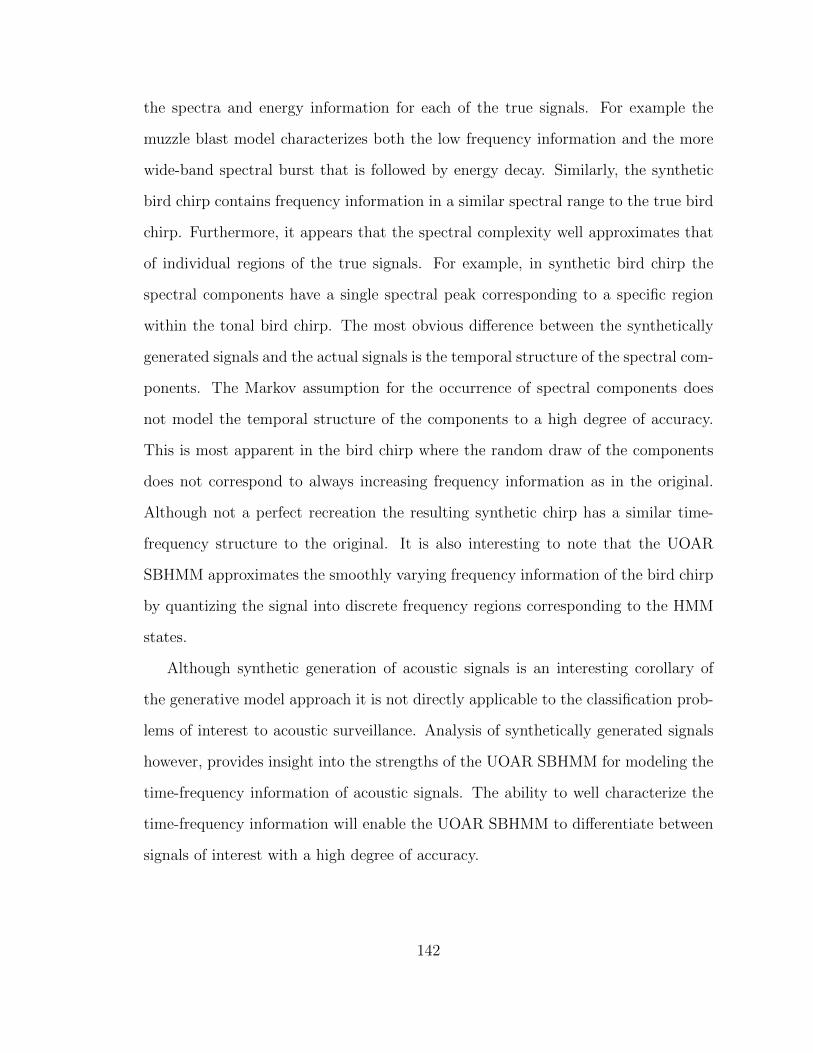
the spectra and energy information for each of the true signals. For example the

muzzle blast model characterizes both the low frequency information and the more

wide-band spectral burst that is followed by energy decay. Similarly, the synthetic

bird chirp contains frequency information in a similar spectral range to the true bird

chirp. Furthermore, it appears that the spectral complexity well approximates that

of individual regions of the true signals. For example, in synthetic bird chirp the

spectral components have a single spectral peak corresponding to a specific region

within the tonal bird chirp. The most obvious difference between the synthetically

generated signals and the actual signals is the temporal structure of the spectral com-

ponents. The Markov assumption for the occurrence of spectral components does

not model the temporal structure of the components to a high degree of accuracy.

This is most apparent in the bird chirp where the random draw of the components

does not correspond to always increasing frequency information as in the original.

Although not a perfect recreation the resulting synthetic chirp has a similar time-

frequency structure to the original. It is also interesting to note that the UOAR

SBHMM approximates the smoothly varying frequency information of the bird chirp

by quantizing the signal into discrete frequency regions corresponding to the HMM

states.

Although synthetic generation of acoustic signals is an interesting corollary of

the generative model approach it is not directly applicable to the classification prob-

lems of interest to acoustic surveillance. Analysis of synthetically generated signals

however, provides insight into the strengths of the UOAR SBHMM for modeling the

time-frequency information of acoustic signals. The ability to well characterize the

time-frequency information will enable the UOAR SBHMM to differentiate between

signals of interest with a high degree of accuracy.

142

5.4.3 Classification of Acoustic Surveillance Signals

In the previous chapter the merits of model order selection for acoustic signal model-

ing were demonstrated by classifying signals of interest to acoustic surverillence using

AR mixture models with varying number of AR orders and numbers of components.

It was shown the the DP mixture of UOAR components was able to obtain equiva-

lent performance to that obtained by the best AR order and number of components

combination. Now, the merit of the inclusion of time dependency for the hidden state

variables is demonstrated by analyzing the same task. Recall, that the dataset is

comprised of data from four acoustic classes, glass breaking, doors slamming, pieces

of wood hitting together, and gunfire. Each of the signals is sampled at 8kHz and

energy normalized. To ensure that the models are not trained and evaluated using

the same data, a five fold cross-validation approach is again utilized.

The posterior density for the parameters of an UOAR SBHMM is determined

using the training examples for each of the classes under consideration. The maxi-

mum number of HMM states was set to S = 25 and the maximum AR order within

each state was set to M = 14. Classification is performed by a assigning a sample of

unknown origin to the class with the maximum posterior probability. Because eval-

uation of this marginal likelihood is intractable, the VB approximate log-likelihood

of each class is utilized instead. The VB approximate log-likelihood for class ω given

example D is

log q (D|c = ω) = Eq(Θω)log f (D|Θω) (5.37)

where Θω represents all of the parameters of the UOAR SBHMM. This can be

evaluated as

log q (D|c = ω) =T∑t=1

S∑i=1

Elog f (st = i)+ Elog f (dt|st = i, θ∗1, . . . , θ

∗S)

(5.38)

143

Figure 5.4: Confusion matrix for the classification of signals relevant to acousticsurveillance. An UOAR SBHMM was used to model acoustic signals from eachclass. The likelihood of each model was used to identify the class of samples withunknown origin. Each element in the matrix shows the percentage of observationsof the corresponding row that were identified as the corresponding column. 93.75%of acoustic signals are correctly identified.

where the θ∗s are evaluated using the model for class ω and the hidden state variables

are estimated using the VB forwards-backwards algorithm.

Classification results are shown as a confusion matrix in Fig. 5.4. Each entry in

the matrix shows the percentage of examples that were identified as the class cor-

responding to the column when they are actually of the class corresponding to the

row. Therefore, the percentages across each row sum to 1. As can be seen, most

of the classes are correctly identified with a high degree of accuracy with only the

examples of wood smashing corresponding being misidentified more than 5 percent of

the time. The difficulty of the wood smashing signals is most likely caused be signif-

144

Figure 5.5: Feature space representation of acoustic surveillance data set. Eachtime-series example is reduced to a point in a two dimensional space through thecalculation of characterizing features. Color and symbol are used to represent thesource of each acoustic signal.

icant changes in the time-frequency spectrum between the different wood-smashing

samples. Overall, the accuracy obtained using the UOAR SBHMM is 93.75%. This

can be compared to the DP mixture of UOAR components analyzed in the last

chapter that obtained only 88.75% correct identification. This indicates that includ-

ing a model for the temporal dependency between the components creates a better

characterizing model and improves performance.

An alternative approach to model based acoustic signal classification is to trans-

form each observation into a set of characterizing features and subsequently apply

one of many standard machine learning techniques to distinguish unknown sam-

ples into one of the specified groups. As discussed in Chapter 1, a number of

previous studies have analyzed feature based classification of acoustic signals (e.g.

[12, 13, 14, 15, 16, 17]). Although employing different features and machine learning

techniques, each of these studies use this approach to perform classification with a

reasonable degree of accuracy. The primary drawback of a feature based approach

is that the specific features and machine learning techniques employed may not be

145

optimal for all types of signals. The desire to have a classification system appropriate

for all types of signals led to the development of the nonparametric signal model in

this chapter.

For comparison purposes, a feature based approach to acoustic signal classifica-

tion is now discussed and applied. A set of features was developed to encapsulate

the spectral and energy characteristics of each of the signals. Ad hoc features such

as the zero crossing rate, the ratio of peak energy to total energy, the location of

the peak energy as a percentage of the total duration and the ratio of second to first

energy peak were used to quantify basic properties of each of the signals. Another

six features were selected to measure spectral properties of the signal; these were the

first three cepstral peak frequencies [87] and the AR weights obtained from maximum

likelihood learning of an AR model of length 3. Finally, two features are derived from

the peak energy from two auditory models. The Lyon auditory model [88] and the

Seneff auditory model [89] are used to provide a measure of the human ability to

perform this task. In total a set of 12 features are calculated for each sample. This

set of features is similar to the features utilized in previous feature based acoustic

classification studies [12, 13, 14, 15, 16, 17]. They include both statistical measures

of the spectrum and intensity of the signal as well as perceptual features. Fig 5.5

shows the resulting feature space after the 12 dimensional feature space is reduced

to 2 dimensions using principal components analysis [31]. The separation and clus-

tering of each of the classes within this feature space shows the appropriateness of

the chosen features.

The relevance vector machine (RVM) [71] was selected as the pattern classifica-

tion technique to be applied to these features. The RVM is a kernel based classifier

which performs sparse Bayesian regression in kernel space as a means of producing a

non-linear decision boundary in feature space. The choice of the particular pattern

classification technique for use on this task is relatively arbitrary. Different pat-

146

tern classification techniques are based on different assumptions and have different

strengths. As a result, the choice of the pattern classification technique which is

best suited to solve a particular problem may require experimental selection. The

RVM was chosen after a comparison of the relative performance of several pattern

classification techniques. The RVM is used to classify the non-binary class problem

by training one RVM to distinguish each class from all other classes and a given

sample is said to belong to the class with maximum a posteriori probability. RVM

based classification results in 85% correct identification compared to the 93.75% ac-

curacy obtained using the UOAR SBHMM. Although it may be possible to improve

performance through modification of the selected feature set or pattern classification

technique, the ability of the UOAR SBHMM to outperform feature based classifica-

tion without specific tuning is note worthy.

5.4.4 Classification of Acoustic Muzzle Blasts

A similar but more difficult acoustic classification problem is now analyzed. The task

is to distinguish between five different types of guns based on their resulting muzzle

blasts. The five guns under consideration are comprised of two handguns, the Glock

model 17 and the Colt Model 1911, and three rifles the Browning FN BAR, the U.S.

M1 Carbine, and the Arisaka Type 38A. Each muzzle blast is sampled at 8kHz and

energy normalized as in the previous analysis. A leave one out cross validation scheme

was utilized to ensure proper evaluation of the performance. The confusion matrix

resulting from classification using the UOAR SBHMM with S = 25 and M = 14 is

shown in Fig 5.6. As can be seen, elements of this dataset can be identified with

a high degree of accuracy (95.65%) as only muzzle blasts from the Arisaka Type

38 rifle are confused as another muzzle blast. The ability of the UOAR SBHMM

to distinguish between acoustic signals with such similar time-frequency structures

motivates the model adaptations that are analyzed in the next chapter. This dataset

147

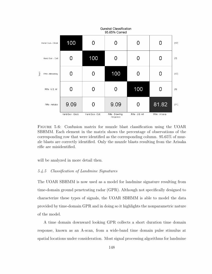
Figure 5.6: Confusion matrix for muzzle blast classification using the UOARSBHMM. Each element in the matrix shows the percentage of observations of thecorresponding row that were identified as the corresponding column. 95.65% of muz-zle blasts are correctly identified. Only the muzzle blasts resulting from the Arisakarifle are misidentified.

will be analyzed in more detail then.

5.4.5 Classification of Landmine Signatures

The UOAR SBHMM is now used as a model for landmine signature resulting from

time-domain ground penetrating radar (GPR). Although not specifically designed to

characterize these types of signals, the UOAR SBHMM is able to model the data

provided by time-domain GPR and in doing so it highlights the nonparametric nature

of the model.

A time domain downward looking GPR collects a short duration time domain

response, known as an A-scan, from a wide-band time domain pulse stimulus at

spatial locations under consideration. Most signal processing algorithms for landmine

148

detection and discrimination utilize the collected A-scans from small spatial regions

to create models for the spatial responses from subsurface objects (e.g. [90, 91]).

Although there is great benefit to utilizing the spatial information across multiple

A-scans, a physical interpretation of the sensing phenomenology indicates that there

may be underutilized information in the time-frequency information contained in

each individual A-scan [92]. Characterizing the time-frequency information of A-

scans from different sub-surface objects has been previously examined [93, 94, 95] but

has seen limited attention due the difficult task of characterizing the rapidly changing

spectral and energy content in the short duration signals. The UOAR SBHMM is well

suited for this task as it is capable of characterizing the time-frequency information

by combining the information in many short duration observations. The application

of the UOAR SBHMM to other time-series data also highlights the generality of the

model. Because the model is nonparametric, and thus performs automated model

order selection, the model is directly applicable to other types of data without any

modifications.

The landmine data under consideration was collected at three test facilities in the

Eastern, central, and Western U.S. from 2006 - 2007. The data set is comprised of

641 responses from 10 different types of landmines. The landmine types are labeled

according to their metal content with three high metal (HM) types, and seven low

metal (LM) types. Prior to analysis, the maximum energy A-scan for each landmine

response is energy normalized as a function of depth using spatially neighboring A-

scans. Fig. 5.7 shows example A-scans from several of the landmine types under

consideration.

The parameters of an UOAR SBHMM were estimated for each mine type in the

dataset using with S = 10 and M = 10. As an example, Fig. 5.8 illustrates the esti-

mated parameters from a HM 1 A-scan. Although there are 10 states in the HMM,

the stick-breaking prior has provided automatic model selection and has only utilized

149

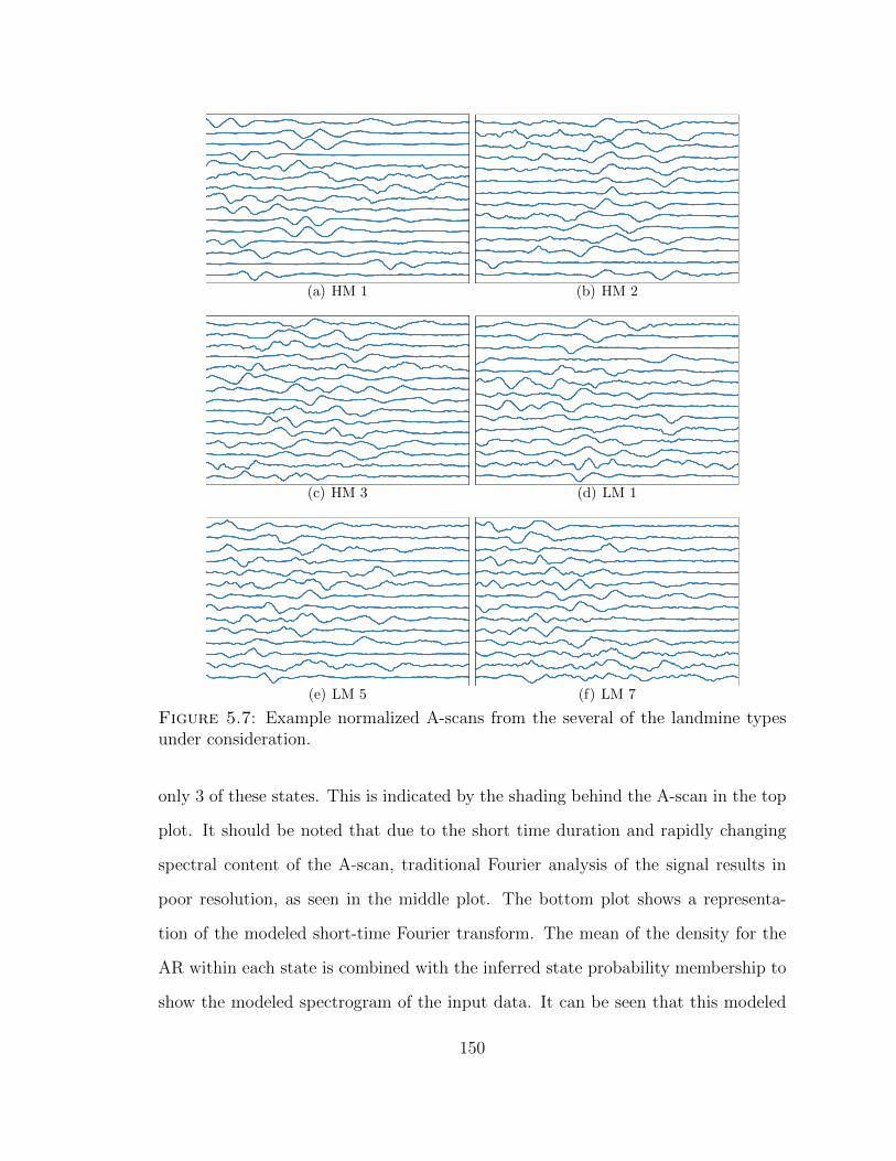
(a) HM 1 (b) HM 2

(c) HM 3 (d) LM 1

(e) LM 5 (f) LM 7

Figure 5.7: Example normalized A-scans from the several of the landmine typesunder consideration.

only 3 of these states. This is indicated by the shading behind the A-scan in the top

plot. It should be noted that due to the short time duration and rapidly changing

spectral content of the A-scan, traditional Fourier analysis of the signal results in

poor resolution, as seen in the middle plot. The bottom plot shows a representa-

tion of the modeled short-time Fourier transform. The mean of the density for the

AR within each state is combined with the inferred state probability membership to

show the modeled spectrogram of the input data. It can be seen that this modeled

150

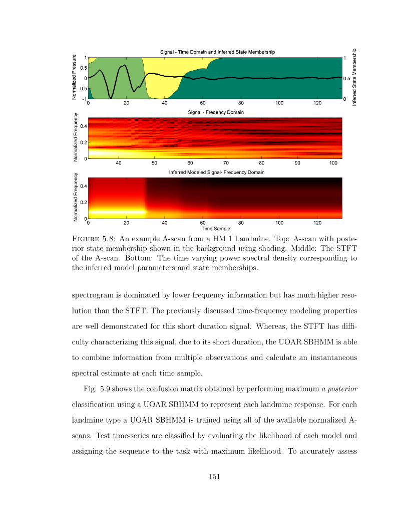
Figure 5.8: An example A-scan from a HM 1 Landmine. Top: A-scan with poste-rior state membership shown in the background using shading. Middle: The STFTof the A-scan. Bottom: The time varying power spectral density corresponding tothe inferred model parameters and state memberships.

spectrogram is dominated by lower frequency information but has much higher reso-

lution than the STFT. The previously discussed time-frequency modeling properties

are well demonstrated for this short duration signal. Whereas, the STFT has diffi-

culty characterizing this signal, due to its short duration, the UOAR SBHMM is able

to combine information from multiple observations and calculate an instantaneous

spectral estimate at each time sample.

Fig. 5.9 shows the confusion matrix obtained by performing maximum a posterior

classification using a UOAR SBHMM to represent each landmine response. For each

landmine type a UOAR SBHMM is trained using all of the available normalized A-

scans. Test time-series are classified by evaluating the likelihood of each model and

assigning the sequence to the task with maximum likelihood. To accurately assess

151

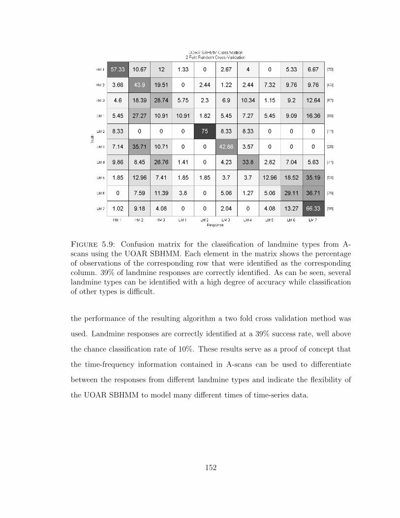
Figure 5.9: Confusion matrix for the classification of landmine types from A-scans using the UOAR SBHMM. Each element in the matrix shows the percentageof observations of the corresponding row that were identified as the correspondingcolumn. 39% of landmine responses are correctly identified. As can be seen, severallandmine types can be identified with a high degree of accuracy while classificationof other types is difficult.

the performance of the resulting algorithm a two fold cross validation method was

used. Landmine responses are correctly identified at a 39% success rate, well above

the chance classification rate of 10%. These results serve as a proof of concept that

the time-frequency information contained in A-scans can be used to differentiate

between the responses from different landmine types and indicate the flexibility of

the UOAR SBHMM to model many different times of time-series data.

152

5.5 Conclusions

This chapter has analyzed the combination of the UOAR model and a nonparamet-

ric approach to hidden Markov modeling that is amenable to variational Bayesian

inference, the SBHMM. The UOAR SBHMM serves as a completely nonparametric

model for acoustic signals. It was demonstrated that the UOAR SBHMM is capable

of characterizing the time-frequency properties of time-series data while remaining

flexible to the types of signals under consideration. It was also demonstrated that

the UOAR SBHMM can be used to classify signals of interest to the acoustic surveil-

lance problem more accurately than the DP mixture of UOAR components analyzed

in the previous chapter and an alternative feature based approach. The flexibility of

the proposed model was then demonstrated through application of the model to the

classification of time-domain GPR signals.

Also in this chapter it was demonstrated that the UOAR SBHMM is able to

distinguish between acoustic signals with very similar time-frequency structure. The

ability to differentiate guns from their muzzle blasts with a high degree of accuracy

motivates the model adaptations undertaken in the next chapter. For the acoustic

sensing task it is often of a interest to develop a model for all types of signals

that one would like to be detected. Because the UOAR SBHMM models the time-

frequency characteristics of a signal, it would be inappropriate to utilize a single

UOAR SBHMM to model a collection of time-series with potentially different time-

frequency structures. To remedy this issue, a nonparametric model for a collection

of time-series that builds upon the developed UOAR SBHMM is developed in the

next chapter,

153

6

Dynamic Nonparametric Modeling for AcousticSignal Classes

The previous two chapters focused on developing and analyzing a nonparametric

model for acoustic signals that is able to distinguish between acoustic signals with

a high degree of accuracy. In Chapter 4 it was demonstrated that Bayesian non-

parametric techniques including the Dirichlet process (DP) and uncertain order au-

toregressive (UOAR) models can be used to perform accurate, automated model

order selection and enable classification performance equivalent to that achieved by

performing a computationally intensive, exhaustive search over all possible model or-

ders. The UOAR model was demonstrated to provide superior model order selection

performance to other model order selection techniques, and shown to provide a mech-

anism to estimate the spectral complexity of time-series data. Furthermore, utilizing

UOAR components within a DP mixture was shown to provide a means to determine

the number of unique spectral and energy components within a signal. In Chapter

5 the nonparametric model was adapted to include a time-structure underlying the

UOAR model components to create a more realistic model for acoustic signals. The

154

resulting model, the UOAR stick-breaking hidden Markov model (SBHMM), was

demonstrated to yield classification performance superior to both standard feature

based approaches to acoustic signal classification and the DP mixture of UOAR

components from Chapter 4.

Also in Chapter 5 it was demonstrated that the UOAR SBHMM is capable of

distinguishing between acoustic signals with very similarly time-frequency structure.

Specifically, in Section 5.4.4 it was demonstrated that muzzle blasts resulting from

different gun types can be distinguished with a high degree of accuracy. For the

acoustic surveillance application of interest in this work, this actually poses a po-

tential problem. Recall that the proposed acoustic surveillance framework utilizes a

two stage approach wherein anomalous acoustic signals are first distinguished from

background acoustic signals and subsequently the signals of interest for a specific

application are distinguished from other anomalous signals. Typically, the goals

of acoustic surveillance are defined not in terms of a specific time-frequency struc-

ture, but instead by a number of time-frequency structures indicative of an class of

acoustic signals, such as “sounds indicative of a security breach” or “muzzle blasts”.

Therefore, the statistical model used to perform classification in the second stage

of processing must be capable of characterizing not just a single but a collection of

time-frequency structures.

A collection of UOAR SBHMMs has been shown to provide a means to perform

classification when the time-frequency structures are specified a priori. However,

acoustic class classification with the UOAR SBHMM requires that either 1) all types

of time-frequency structures within a specific class are assumed to be modeled by

the same UOAR SBHMM, or 2) every possible time-frequency structure within a

class are known a priori and specified when the algorithm is trained. Both of these

approaches are inadequate for robust fielded performance. The first option violates

the assumptions made when applying the UOAR SBHMM to acoustic signal mod-

155

eling. Consider the bird chirp modeling example from Fig. 5.3(b). If it is desired

to detect the abstract acoustic class of bird chirps, perhaps for ecological purposes,

it is undesirable to model bird chirps that exhibit a rising chirp structure and those

exhibiting a falling chirp structure with the same UOAR SBHMM, as the temporally

changing nature of the frequency components is modeled by the transition proba-

bilities of the HMM. By combining both of these structures into a single HMM, the

transition information is aggregated across both sequences and therefore the model

does not characterize either type of chirp well. The second option to utilize the

UOAR SBHMM to model acoustic signal classes requires that time-frequency struc-

tures be enumerated and all examples be labeled prior to algorithm training. This

task appears manageable when considering the class of muzzle blasts, however, the

methodology quickly becomes impractical when considering the bird chirp example.

The entire collection of bird chirps to be used to train the system would need to be

artificially partitioned into groups with similar time-frequency structure. Once this

is accomplished, there is no indication that the collection of signals would not be

better modeled by splitting or combining some of the specified groups. Therefore,

performance of the algorithm is tied to the ad hoc artificial partitioning.

This chapter offers an alternative methodology that allows the use of the UOAR

SBHMM to model classes of acoustic signals. Specifically, the new model is real-

ized by considering the UOAR SBHMM as the base distribution for a DP mixture

and assuming that each acoustic time-series is generated by an UOAR SBHMM.

Parameter inference for this model inherently clusters all time-series into groups

that share common time-frequency characteristics while simultaneously learning an

UOAR SBHMM to model the data within each group. Because the top level model

is a DP mixture, the number of unique time-frequency structures is inferred from

the data and because each group is modeled using an UOAR SBHMM the num-

ber of unique spectral components and the spectral complexity of each component

156

within each time-frequency model is also inferred. Therefore, the model is a fully

nonparametric Bayesian approach to modeling a collection of time-series that may

have different time-frequency structures. Because the model automatically performs

a clustering of the input training data the modeled is referred to as nonparametric

Bayesian time-series clustering (NPBTSC).

Relating back to the classification example above, the clustering properties of the

NPBTSC model can be seen as an automated method to partition a collection of bird

chirps into groups with similar time-frequency properties. Therefore, an algorithm to

discriminate between an acoustic signal class of interest, such as bird chirps, from all

other anomalous signals requires only partitioning the collection of training examples

into these two classes. Not only does this eliminate the necessity to group and label

all examples in the dataset but it also provides a more accurate model as the samples

are automatically grouped by virtue of the models used to characterize them.

This chapter begins by developing a variational Bayesian (VB) learning proce-

dure for the NPBTSC model and then it is demonstrated how NPBTSC can be used

to cluster and model a collection of acoustic signals. This is illustrated first using

the collection of muzzle blasts analyzed in the previous chapter. The determined

clusterings are related back to the classification results from Section 5.4.4 and the

classification errors are seen to correspond to different time-frequency characteristics

within the muzzle blasts from a particular gun type, validating the choice to perform

automatic clustering rather than utilize a pre-specified grouping to define a collec-

tion of UOAR SBHMMs. Following this, the nonparametric nature of the model is

again highlighted through analysis of the ground penetrating radar (GPR) landmine

signature dataset analyzed in the previous chapter. Here the landmine signatures

are modeled and clustered using NPBTSC and the resulting clustering is related to

known physical characteristics of the landmines and soils to determine the factors

that govern the time-frequency characteristics of GPR signatures.

157

Following this, the NPBTSC model is used to perform discrimination between

two classes of acoustic signals, the collection of muzzle blasts and the collection

of other anomalous acoustic signals analyzed in Chapters 4 and 5. Classification

performance provided by the NPBTSC is compared to utilizing an UOAR SBHMM

to model each class of acoustic signals (option 1 from above). Although both models

perform favorably, the NPBTSC model outperforms single UOAR SBHMM modeling

in addition to corresponding more closely with intuition and ultimately enabling

algorithmic adaptation.

One of the primary goals of the acoustic sensing framework analyzed throughout

this work is to develop an algorithm that is capable of adapting to changing envi-

ronmental and operating conditions. This requirement has lead to use of Bayesian

parameter estimation, specifically the use of conjugate priors and the VB method,

throughout this work. Finally, in this chapter the ability of the NPBTSC model

for an acoustic signal class to adapt when new data is received is realized. Recall

the example of a vehicle mounted gunshot detection system from Chapter 1. As the

vehicle moves to new locations the specific types of guns in use may change or a new

type of gun not yet known to the system may be encountered. Because the NPBTSC

model is estimated using the VB method it has a parameterized posterior density of

the same functional form of the prior density and therefore it provides a principled

method to update the probability density for a class of acoustic signals. To achieve

adaptibility, in this chapter a learning algorithm for dynamic NPBTSC is devel-

oped and analyzed wherein a posterior NPBTSC density is updated with new data.

Although there are some application specific implementation details the NPBTSC

model provides a straight-forward and principled method to meet the desired goal of

algorithmic adaptation.

158

6.1 Nonparametric Bayesian Time Series Clustering

The UOAR SBHMM has been established as a statistical model that is capable

of characterizing the time-frequency information of acoustic signals. It is therefore

natural to include the UOAR SBHMM as a building block within a larger statistical

model to create a model for a collection of time-series data. An intuitive description

of the proposed model is as follows. Each times-series can be thought of as an

example drawn from one of a collection of time-series structures. Each time-series

structure is modeled as an UOAR SBHMM and therefore the model can be realized

as a probabilistic mixture of HMMs.

Probabilistic mixtures of HMMs have previously been examined in the context

of acoustic signal classification, specifically for music analysis [27, 28, 29]. In these

examples, a music analysis problem in which the goal is to determine the similarity

between pieces of music is examined. The acoustic signal for each piece of music is

transformed and quantized into a set of discrete Mel-frequency cepstral coefficients

and each is modeled as a mixture of HMMs with discrete observation densities. As

mention previously, this transformation is inappropriate for the application indepen-

dent approach taken in this work. Therefore, the model developed in this chapter

utilizes the UOAR model as the observation density within each HMM state and

therefore is significantly different than the approach taken to acoustic signal model-

ing in these aforementioned works.

Another significant difference between the models presented in [27, 28, 29] and

the model presented in this chapter is the manner in which the probabilistic mixing

is assumed to occur within the data. In [27, 28, 29] a piece of music is modeled as a

number of sections, and each section is modeled using an HMM. Therefore, a single

sequence of music is modeled using a mixture of HMM and each observation in the

sequence can originate from either of the HMMs. In the NPBTSC model developed

159

here, a given sequence is assumed to originate from a single HMM, an assumption

fitting the acoustic signal class modeling application of interest.

The proposed NPBTSC model also uses probabilistic structures based on the

DP and the stick-breaking construction to provide automatic model order selection

of the number of required HMMs and the number of states within each HMM and

utilizes the VB method to infer the posterior density of the model parameters. The

models presented in [27, 28, 29] differ in the assumptions made regarding the number

of HMMs and the number of states within each HMM as well as the method of

approximate Bayesian inference. The model and inference algorithm presented in

[29] is most similar to that presented here in that both the number of HMMs and

the number of states within each HMM are modeled using nonparametric Bayesian

methodology and the VB method is used for parameter inference. However, the

model in [29] is still significantly different from the proposed model due to previously

mentioned manner of mixing at the time-series level rather than the sample level and

more importantly the use of the UOAR model to create a fully nonparametric model.

Because the NPBTSC model assumes that each time-series originates from a sin-

gle UOAR SBHMM, performing parameter inference for the model automatically

clusters the sequences that share common UOAR SBHMM parameters. The task

of clustering a group of time-series utilizing AR models has also been previously

examined. In [66] and [96] a mixture of AR models are used to cluster sequences.

However, each time-series cluster is characterized by a single AR model and param-

eter inference is done using the expectation maximization algorithm with a fixed

number of clusters and a fixed AR order. Characterizing each sequence with a single

set of spectral and energy characteristics is insufficient for many applications. An-

other similar approach to sequence clustering is shown in [97] wherein a HMM is

used to model each sequence. However, a mixture of HMMs is not considered, only

a hard clustering, and the number of clusters as well as the number of states in the

160

HMMs are assumed fixed and known. The model proposed here is different from

these previous approaches to time-series clustering in that it is nonparametric: both

the model for each time-series type as well as the total number of distinct time-series

types are determined by the data.

6.1.1 Model

Recall that a DP mixture model assumes that a mixing distribution G is a draw

from a DP and therefore is a discrete probability density function that assigns mass

to infinite number of points drawn from the base density of the DP, G0, denoted in

this chapter as Θ∗i .

G =∞∑i=1

πiδΘ∗i(6.1)

In Chapter 4 a DP mixture of UOAR components is realized by assuming that G0

is a discrete-Normal-inverse-Wishart density and therefore each Θ∗i corresponds to a

draw from this density, an AR order, a set of AR weights, and an innovations power.

Using the stick-breaking construction a VB learning procedure can be utilized to

provide a parameterized posterior density that approximates the infinite mixture

model. In Chapter 4 it was demonstrated how this model can be used to accurately

estimate the number of AR components in a mixture AR model. This same type of

methodology is employed in this chapter to create a model for a collection of time-

series that can automatically determine the number of distinct types of time-series

within the training data.

The collection of time-series in the dataset are denoted as di for i ∈ 1, 2, . . . , N

and the number of samples in each is donated as Ti, di = [di,1, di,2, . . . , di,Ti ]′. In the

previous chapter the UOAR SBHMM was established as a nonparametric Bayesian

model that is capable of characterizing the time-frequency characteristics of an acous-

tic time-series. Therefore, it can be assumed that each time series is modeled as an

161

UOAR SBHMM with parameter set Θi. If it is assumed that the Θi are drawn from

Polya urn scheme, and thus the underlying mixing distribution for the collection

of time-series is a draw from a DP, the collection of time-series will be defined by

a unique subset of the UOAR SBHMM parameter sets Θ∗j . As in a standard DP

mixture model, an index zi can be used to indicate which Θi = Θ∗zi and the indexes

can be viewed as a partition of the collection of time-series into clusters. In relation

to the underlying DP, this model states that the mixing distribution G places mass

to an infinite number of UOAR SBHMM parameter sets, and is itself a draw from a

DP in which the base distribution G0 is the UOAR SBHMM prior structure, from

(5.10),

f (·) = f(stT1

) S∏i=1

βρ0,i

(γ0

0,i,1, γ00,i,2

)

·S∏i=1

S∏j=1

βρi,j(γ0i,j,1, γ

0i,j,2

)

·S∏i=1

M∑l=1

µ0i,lN iGai,ll,ri,l

(ν0i,l,V

0i,l

). (6.2)

The use of a model with an infinite model order as a base density for another

model with infinite model order is referred to in statistics as a nested model [98].

This is significantly different from the hierarchical DP discussed in the previous

chapter, wherein a draw from a DP is used as the base density of another DP. In

the case of a nested DP, a DP mixture model, not a draw from a DP, is used as the

base density of each inner layer. Models of this type have been utilized to model a

collections of documents [99] and other data collections that are to be clustered by

a common probability density function that is itself hierarchical or nested in nature

[100]. It is therefore appropriate to utilize a nested model structure based on the

UOAR SBHMM to create a model for a collection of time-series that will cluster the

162

time-series based on their time-frequency characteristics.

Denoting the probability that any sequence is generated by UOAR SBHMM

parameter set Θ∗j as πz,j and the vector of these probabilities as πz, the generative

process for the ith sequence can be written as follows

di ∼ fdi (Θzi)

zi ∼Multi (πz)

πz = SB (τ )

τj ∼ β (κj,1, κj,2) (6.3)

where κj,1 and κj,2 have been used to denote the parameters of the beta density

governing the stick proportion τj, for j ∈ 1, 2, . . . , J the collection of which are

used to determine πz. Given the set of UOAR SBHMM parameters for the ith

sequence Θ∗zi the samples of the ith sequence can be drawn using the generative

process for the UOAR SBHMM discussed in Chapter 5. The prior for the entire

model is then given by

f (·) = f(ziNi=1

) J∏i=1

βτi(κ0i,1, κ

0i,2

) J∏i=1

f (Θ∗i ) (6.4)

where each f (Θ∗i ) corresponds to prior shown in (6.2).

To summarize, the DP mixture of UOAR SBHMM models a collection of time

series, each denoted as di, and will cluster these time-series into at most J groups,

with the number of groups in use determined by the dataset. Each group is mod-

eled by an UOAR SBHMM. Each UOAR SBHMM is comprised of a maximum of

S states the number of which in use will be determined by the data and within

each state, the appropriate AR order (from 1 to M) will also be determined by

the data. As mentioned previously, due to the inherent clustering of the time-series

accomplished by this model, it will refer to as nonparametric Bayesian time-series

clustering (NPBTSC).

163

6.1.2 Model Inference

To provide a parameterized posterior density to enable the recursive Bayesian es-

timation analyzed below the VB method is once again utilized. The variational

approximate posterior density is assumed to be factored as

q (·) = q(ziN1

) J∏i=1

βτi (κi,1, κi,2)

J∏i=1

q (Θ∗i ) (6.5)

where q (Θ∗i ) is the approximate posterior structure for the UOAR SBHMM from

(5.11),

q (·) = q(stT1

) S∏i=1

βρ0,i (γ0,i,1, γ0,i,2)

·S∏i=1

S∏j=1

βρi,j (γi,j,1, γi,j,2)

·S∏i=1

M∑l=1

µi,lN iWai,l,ri,l (νi,l,Vi,l). (6.6)

The learning procedure resulting from application of the VB method results in an

algorithm similar to a standard DP mixture coupled with the learning procedure

for UOAR SBHMM discussed in the previous chapter. The primary difference from

estimating the posterior density of a single UOAR SBHMM is that in the NPBTSC

model each of the parameters of the J UOAR SBHMMs are estimated using all N of

the available sequences with the influence of each sequence on each UOAR SBHMM

determined by q (zi).

Following initialization (discussed below), each iteration of the VB procedure be-

gins by estimating the group membership for each sequence to each group q (zi = j).

This is determined by

log q (zi = j) ∝ Elog πz,j+ Elog f(di,Θ

∗j

) (6.7)

164

where the expected values are taken with respect to the current approximate density

for all parameters except for q (zi = j). The first term can be determined from the

current values of κ1 and κ2 using the moments of the beta density and the definition

of the stick-breaking construction

Elog τi = ψ (κi,1)− ψ (κi,1 + κi,2)

Elog (1− τi) = ψ (κi,2)− ψ (κi,1 + κi,2)

Elog πz,i = Elog τi+i−1∑k=1

Elog (1− τk). (6.8)

The second term is calculated as part of the negative free energy when learning a

single UOAR SBHMM. This is the first term of (5.36) indexed by the jth UOAR

SBHMM

Ti∑t=1

S∑k=1

Elog f

(sji,t = k

)+ Elog f

(di,t|sji,t = k, θ∗j,1, . . . , θ

∗j,S

). (6.9)

Therefore, this quantity can be calculated using the outputs of VB forward backwards

for the ith sequence with the jth UOAR SBHMM hyperparameters.

Determining q (zi = j) at each iteration is equivalent to performing a soft cluster-

ing of the N sequences into the J groups with the possibility that some of the groups

are empty, thus performing automated model selection. Following this, the expected

number of sequences in the jth group uj can be determined through summation

uj =N∑i=1

q (zi = j) . (6.10)

Using this quantity the parameters for the beta densities governing the stick-breaking

proportions for determining πz can be re-estimated

κj,1 = κ0j,1 + uj (6.11)

κj,2 = κ0j,2 +

J∑k=j+1

uk. (6.12)

165

The above steps are the same methodology used to estimate a standard DP

mixture model with components specified by parameter sets Θ∗j . The primary change

to include the UOAR SBHMM thus far has been in (6.7) where the variational average

log likelihood for the UOAR SBHMM is utilized. Now the primary calculation for

use of an UOAR SBHMM based density must be considered: the parameters for

the UOAR SBHMM for each group must be re-estimated using the current group

memberships q (zi = j). This is done for each UOAR SBHMM independently using

all sequences. Considering specifically the jth sequence, the first step is to determine

the approximate posterior for the hidden state sequence for each of the N time-series,

q(sji,t

Tit=0Ni=1

). This can be accomplished by using the VB forwards backwards

algorithm for each time-series using the parameters of the jth UOAR SBHMM model,

in a similar manner as in Chapter 5. The VB forward-backwards algorithm on each

of the J UOAR SBHMMs will thus estimate both the probability that the hidden

state for the tth sample of the ith time series in group j is state k, q(sji,t = k

)for all

combinations of i ∈ 1, . . . , N, t ∈ 1, . . . , Ti, k ∈ 1, . . . , S, and j ∈ 1, . . . , J,

and the expected probability of transitioning from state k to k′ at each time for each

observation sequence within each UOAR SBHMM, ξji,t (k, k′).

Using q(sji,t = k

)the discrete-Normal-inverse-Wishart density governing the statis-

tics within state k of the jth group model can be determined in a manner similar to

performing inference for a single UOAR SBHMM. The total density for the dataset

assuming all the hidden indicator variables zi are known is

N∏i=1

J∏j=1

(f(di|Θ∗j

))δzi,j (6.13)

where δa,b indicates a Kronecker delta function that is equal to 1 when a and b are

equal and zero otherwise. This definition also assumes that the hidden state sequence

166

is also known. More explicitly the density for the dataset is

N∏i=1

J∏j=1

(Ti∏t=1

S∏k=1

(f(di,t|θ∗j,k

))δsji,t,k

)δzi,j

. (6.14)

Recall that utilizing the VB method to update the parameters for each state within a

single UOAR SBHMM results in weighting the influence each data sample using the

current posterior density of the hidden state parameters (see (5.32) and (5.33)). Be-

cause of the exponential relationship between the indicator variables, the parameters

within each state of each UOAR SBHMM in the NPBTSC model can be updated

using the same methodology by weighting each data sample by the product of the

posterior density for the two types of indicator variables. The probability of sample

t of sequence di belonging to hidden state k of group j is then the product of the

two determined membership probabilities ωi,t,j,k = q(sji,t = k

)q (zi = j). Using this

probability, the Normal-inverse-Wishart parameters for AR order l can be deter-

mined as before by replacing q (st = i) in (5.32) and (5.33) with ωi,t,j,k and including

each sequence in the summations.

Vj,k,l = V0l +

N∑i=1

Ti∑t=1

ωi,t,j,kφli,t

(φli,t)′

(6.15)

νj,k,l = ν0l +

N∑i=1

Ti∑t=1

ωi,t,j,k. (6.16)

The AR order probability vector can also be determined as before by using the

appropriate sets of Normal-inverse-Wishart parameters.

µj,k,l ∝ µ0l

Z (Vj,k,l, νj,k,l)

Z (V0l , ν

0l )

. (6.17)

After the parameters for the state densities within each state of each group model,

the parameters for the transition probabilities and the initial state probabilities must

167

be re-estimated. Once again the necessary quantities to re-estimate these are deter-

mined from the outputs of the VB forward-backwards algorithm for each sequence

with each UOAR SBHMM. The expected number of transitions from state k to state

k′ for model j, njk,k′ can be determined as

njk,k′ =N∑i=1

Ti∑t=1

ξji,t (k, k′) . (6.18)

Using these variables, the set of stick-breaking beta density parameters for SBHMM

j can be determined as follows

γj,k,k′,1 = γ0k,k′,1 + njk,k′ (6.19)

γj,k,k′,2 = γ0k,k′,2 +

S∑c=k′+1

njk,c. (6.20)

Updating the stick-breaking proportion beta densities concludes one iteration of the

algorithm.

As in all VB learning procedures, convergence can be monitored by calculating

the negative free energy, F (·), after each iteration. For the NPBTSC model, the

negative free energy can be shown to be

F =N∑i=1

J∑j=1

Elog πz,j+ Elog f (di|zi = j,Θ∗1, . . . ,Θ

∗J)

−J∑j=1

KL(q(Θ∗j)||p(Θ∗j))−

J∑j=1

KL (q (τj) ||p (τj)) . (6.21)

The first term is the average variational log-likelihood of the entire collection of time-

series which can be determined using the average variational log-likelihoods used to

determine the hidden state sequences and the current estimate of group probabilities.

The final term is a sum of Kullback Leibler divergences (KLDs) between the posterior

beta densities for the stick propotions τ and the prior densities. The second term

168

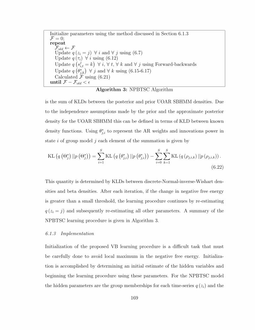
Initialize parameters using the method discussed in Section 6.1.3F = 0;repeatFold ← FUpdate q (zi = j) ∀ i and ∀ j using (6.7)Update q (τi) ∀ i using (6.12)Update q

(sji,t = k

)∀ i, ∀ t, ∀ k and ∀ j using Forward-backwards

Update q(θ∗j,k)∀ j and ∀ k using (6.15-6.17)

Calculated F using (6.21)until F − Fold < ε

Algorithm 3: NPBTSC Algorithm

is the sum of KLDs between the posterior and prior UOAR SBHMM densities. Due

to the independence assumptions made by the prior and the approximate posterior

density for the UOAR SBHMM this can be defined in terms of KLD between known

density functions. Using θ∗j,i to represent the AR weights and innovations power in

state i of group model j each element of the summation is given by

KL(q(Θ∗j)||p(Θ∗j))

=S∑i=1

KL(q(θ∗j,i)||p(θ∗j,i))−

S∑i=0

S∑k=1

KL (q (ρj,i,k) ||p (ρj,i,k)) .

(6.22)

This quantity is determined by KLDs between discrete-Normal-inverse-Wishart den-

sities and beta densities. After each iteration, if the change in negative free energy

is greater than a small threshold, the learning procedure continues by re-estimating

q (zi = j) and subsequently re-estimating all other parameters. A summary of the

NPBTSC learning procedure is given in Algorithm 3.

6.1.3 Implementation

Initialization of the proposed VB learning procedure is a difficult task that must

be carefully done to avoid local maximum in the negative free energy. Initializa-

tion is accomplished by determining an initial estimate of the hidden variables and

beginning the learning procedure using these parameters. For the NPBTSC model

the hidden parameters are the group memberships for each time-series q (zi) and the

169

hidden state sequences for each time-series and for each group model q(sji,t). As

stated previously, estimating q (zi) is equivalent to clustering the time-series into J

groups according to their time-frequency characteristics. To begin the initialization,

a similar methodology to that presented for model based sequence clustering in [97] is

utilized. First, an UOAR SBHMM is estimated for each sequence independently and

the average variational log-likelihood of each sequence is evaluated using the mode

for every other sequence. This creates a similarity matrix, an example of which is

shown in Fig. 6.1(b). Following this, a KLD based approach is used to normalize and

transform the similarity matrix into a distance matrix and agglomerative clustering

is applied [97]. An example of the distance matrix that is used for agglomerative

clustering is shown in Fig. 6.1(b). After this step the N time-series are clustered

into J groups and thus an initial q (zi) can be determined.

Next an initial hidden state sequence for each time-series within each group model

is required. Each hidden state sequence can be determined through the use of the VB

forward-backwards algorithm if initial parameters for each UOAR SBHMM are first

determined. Each UOAR SBHMM is initialized using the initialization procedure

and one iteration of the VB learning algorithm for the UOAR SBHMM described in

Chapter 5. The parameters for the UOAR SBHMM for group j are initialized using

only the time-series that were assigned to group j by the clustering performed above.

Once each UOAR SBHMM has been initialized, the VB forward-backwards algorithm

can by run with each time-series and model combination to determine an initial

value for q(sji,t). Now, with values determined for q (zi) and q

(sji,t)

the VB learning

procedure begins by first estimating the stick-breaking proportion parameters and

then continuing as described above.

170

6.1.4 Prior Parameters

As has been the case throughout this research, the prior parameters are selected to

have minimal effect on the resulting learned parameters. The parameters of V0l and

ν0l are selected as in Chapters 4 and 5 to correspond to AR weights with zero mean

and a diagonal covariance matrix with variance 1000 and an innovations power with a

mean of 1 and a variance of 1000. The values of γ0i,j,1 and γ0

i,j,2, control the preference

for sparsity in the number of states within a HMM. As in the previous chapter these

parameters were set to 2 and 1 respectively and not tuned relative to data. The

values of κ0i,1 and κ0

i,2 control the sparsity for the number of time-series clusters.

These values were also set to 2 and 1 and not tuned relative to data. In practice

these values can be altered to represent prior information regarding the number of

unique time-series types within the dataset. Alternatively a Gamma prior could be

used for κ0i,1 to represent the uncertainty in this parameters, as was done for the DP

mixture considered in Chapter 4, although this is not done for the NPBTSC model

in this work.

6.1.5 Example

The VB learning procedure for the NPBTSC model is now illustrated on synthetic

data to provide insight into the methodology and the expected behavior of the al-

gorithm. First, two UOAR SBHMMs were specified and 25 2000 sample sequences

were generated by selecting between the two time-series models with equal probabil-

ity. The first time-series model has two AR states and with transitions between the

two states occurring with a probability of 0.005 for each sample. The first state has

two spectral peaks with normalized frequencies of 0.2 and 0.7 with an innovations

power of 1 and the second state has two spectral peaks with normalized frequencies

of 0.1 and 0.6 with an innovations power of 2. The second time-series model has

three HMM states with a self transition probability of 0.995 and an equal transition

171

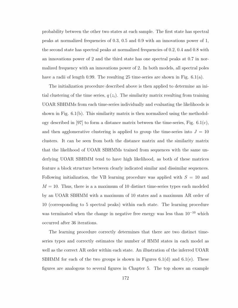
probability between the other two states at each sample. The first state has spectral

peaks at normalized frequencies of 0.3, 0.5 and 0.9 with an innovations power of 1,

the second state has spectral peaks at normalized frequencies of 0.2, 0.4 and 0.8 with

an innovations power of 2 and the third state has one spectral peaks at 0.7 in nor-

malized frequency with an innovations power of 2. In both models, all spectral poles

have a radii of length 0.99. The resulting 25 time-series are shown in Fig. 6.1(a).

The initialization procedure described above is then applied to determine an ini-

tial clustering of the time series, q (zi). The similarity matrix resulting from training

UOAR SBHMMs from each time-series individually and evaluating the likelihoods is

shown in Fig. 6.1(b). This similarity matrix is then normalized using the methodol-

ogy described in [97] to form a distance matrix between the time-series, Fig. 6.1(c),

and then agglomerative clustering is applied to group the time-series into J = 10

clusters. It can be seen from both the distance matrix and the similarity matrix

that the likelihood of UOAR SBHMMs trained from sequences with the same un-

derlying UOAR SBHMM tend to have high likelihood, as both of these matrices

feature a block structure between clearly indicated similar and dissimilar sequences.

Following initialization, the VB learning procedure was applied with S = 10 and

M = 10. Thus, there is a a maximum of 10 distinct time-series types each modeled

by an UOAR SBHMM with a maximum of 10 states and a maximum AR order of

10 (corresponding to 5 spectral peaks) within each state. The learning procedure

was terminated when the change in negative free energy was less than 10−10 which

occurred after 36 iterations.

The learning procedure correctly determines that there are two distinct time-

series types and correctly estimates the number of HMM states in each model as

well as the correct AR order within each state. An illustration of the inferred UOAR

SBHMM for each of the two groups is shown in Figures 6.1(d) and 6.1(e). These

figures are analogous to several figures in Chapter 5. The top shows an example

172

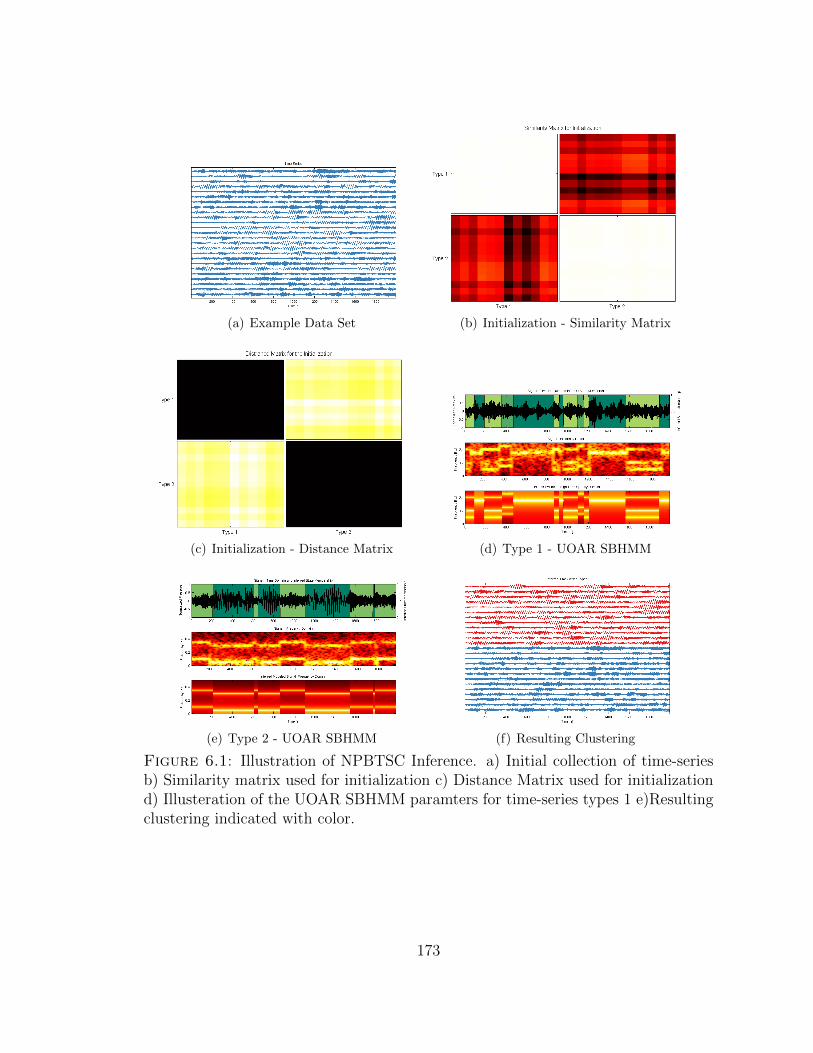
(a) Example Data Set (b) Initialization - Similarity Matrix

(c) Initialization - Distance Matrix (d) Type 1 - UOAR SBHMM

(e) Type 2 - UOAR SBHMM (f) Resulting Clustering

Figure 6.1: Illustration of NPBTSC Inference. a) Initial collection of time-seriesb) Similarity matrix used for initialization c) Distance Matrix used for initializationd) Illusteration of the UOAR SBHMM paramters for time-series types 1 e)Resultingclustering indicated with color.

173

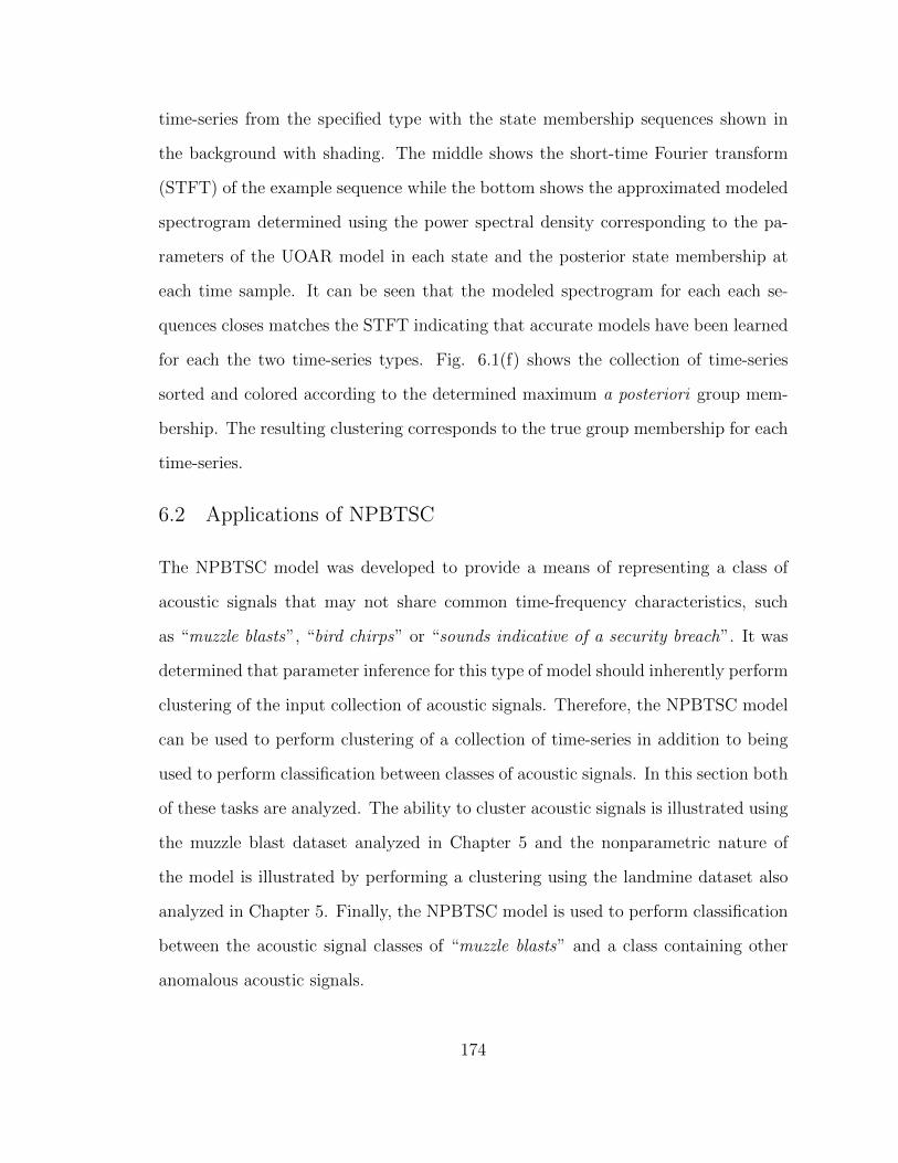
time-series from the specified type with the state membership sequences shown in

the background with shading. The middle shows the short-time Fourier transform

(STFT) of the example sequence while the bottom shows the approximated modeled

spectrogram determined using the power spectral density corresponding to the pa-

rameters of the UOAR model in each state and the posterior state membership at

each time sample. It can be seen that the modeled spectrogram for each each se-

quences closes matches the STFT indicating that accurate models have been learned

for each the two time-series types. Fig. 6.1(f) shows the collection of time-series

sorted and colored according to the determined maximum a posteriori group mem-

bership. The resulting clustering corresponds to the true group membership for each

time-series.

6.2 Applications of NPBTSC

The NPBTSC model was developed to provide a means of representing a class of

acoustic signals that may not share common time-frequency characteristics, such

as “muzzle blasts”, “bird chirps” or “sounds indicative of a security breach”. It was

determined that parameter inference for this type of model should inherently perform

clustering of the input collection of acoustic signals. Therefore, the NPBTSC model

can be used to perform clustering of a collection of time-series in addition to being

used to perform classification between classes of acoustic signals. In this section both

of these tasks are analyzed. The ability to cluster acoustic signals is illustrated using

the muzzle blast dataset analyzed in Chapter 5 and the nonparametric nature of

the model is illustrated by performing a clustering using the landmine dataset also

analyzed in Chapter 5. Finally, the NPBTSC model is used to perform classification

between the acoustic signal classes of “muzzle blasts” and a class containing other

anomalous acoustic signals.

174

6.2.1 Clustering Acoustic Muzzle Blasts

In Section 5.4.4 a collection of muzzle blasts from four different guns was analyzed

and an UOAR SBHMM was utilized to model the muzzle blasts from each gun. The

classification results obtained from an appropriate cross-validation procedure showed

that the UOAR SBHMM is able to characterize muzzle blasts from three of the gun

types with a high degree of accuracy, however, the muzzle blasts from one type of

gun were not modeled as accurately and as a result muzzle blasts from this gun

type were not classified as accurately. The NPBTSC model is now applied to this

same dataset to illustrate the ability of the model to cluster acoustic signals and the

resulting clustering illustrates why one particular type of gun was difficult to classify.

The NPBTSC model was applied to the dataset allowing for a maximum of J = 25

unique time-series types and using an UOAR SBHMM with S = 25 possible HMM

states with a highest possible AR order of M = 14 within each state. Fig. 6.2

shows the distance matrix that is used in the initialization process of the NPBTSC

learning procedure. Recall that this distance matrix is calculated by first estimating

the parameters of a UOAR SBHMM for each sequence and evaluating the likelihood

of each sequence using each estimated model and then applying the methodology

in [97] to transform this similarity matrix to a distance matrix. Each row and each

column in the distance matrix corresponds to a time-series in the data collection

and therefore each pixel indicates the distance between each pair of sequences in the

dataset. Dark colors are used to indicate similarity while light colors are used to

indicate dissimilarity. The time-series are grouped according to their underlying gun

type and each group is separated to highlight the block diagonal nature appearance

of the distance matrix.

From Fig. 6.2 it can be seen that there is a high degree of within type similarity

between muzzle blasts from the three types of guns that are well classified using

175

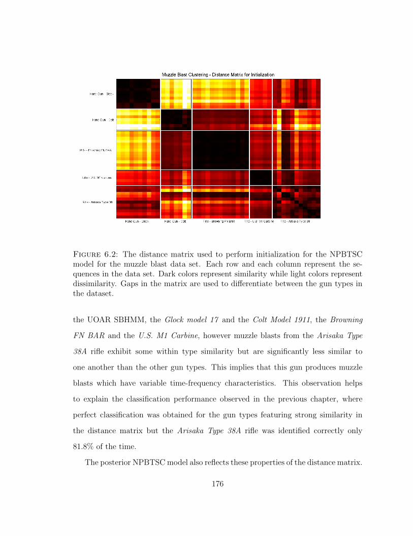
Figure 6.2: The distance matrix used to perform initialization for the NPBTSCmodel for the muzzle blast data set. Each row and each column represent the se-quences in the data set. Dark colors represent similarity while light colors representdissimilarity. Gaps in the matrix are used to differentiate between the gun types inthe dataset.

the UOAR SBHMM, the Glock model 17 and the Colt Model 1911, the Browning

FN BAR and the U.S. M1 Carbine, however muzzle blasts from the Arisaka Type

38A rifle exhibit some within type similarity but are significantly less similar to

one another than the other gun types. This implies that this gun produces muzzle

blasts which have variable time-frequency characteristics. This observation helps

to explain the classification performance observed in the previous chapter, where

perfect classification was obtained for the gun types featuring strong similarity in

the distance matrix but the Arisaka Type 38A rifle was identified correctly only

81.8% of the time.

The posterior NPBTSC model also reflects these properties of the distance matrix.

176

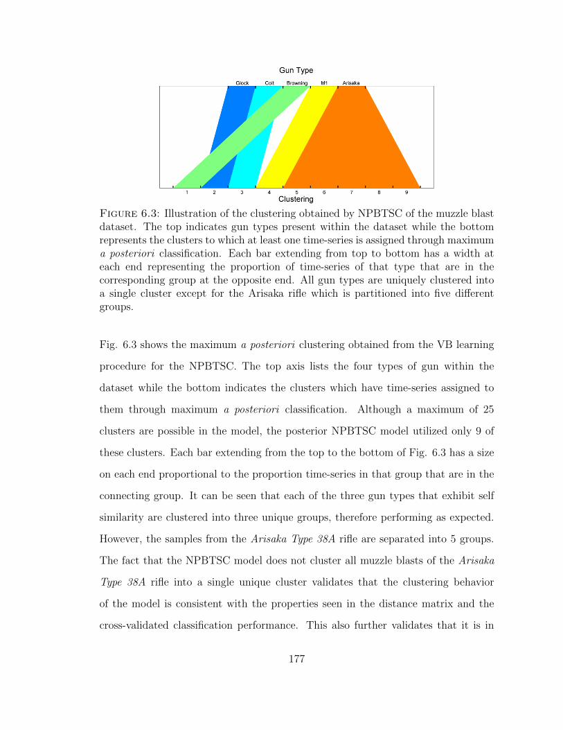
Figure 6.3: Illustration of the clustering obtained by NPBTSC of the muzzle blastdataset. The top indicates gun types present within the dataset while the bottomrepresents the clusters to which at least one time-series is assigned through maximuma posteriori classification. Each bar extending from top to bottom has a width ateach end representing the proportion of time-series of that type that are in thecorresponding group at the opposite end. All gun types are uniquely clustered intoa single cluster except for the Arisaka rifle which is partitioned into five differentgroups.

Fig. 6.3 shows the maximum a posteriori clustering obtained from the VB learning

procedure for the NPBTSC. The top axis lists the four types of gun within the

dataset while the bottom indicates the clusters which have time-series assigned to

them through maximum a posteriori classification. Although a maximum of 25

clusters are possible in the model, the posterior NPBTSC model utilized only 9 of

these clusters. Each bar extending from the top to the bottom of Fig. 6.3 has a size

on each end proportional to the proportion time-series in that group that are in the

connecting group. It can be seen that each of the three gun types that exhibit self

similarity are clustered into three unique groups, therefore performing as expected.

However, the samples from the Arisaka Type 38A rifle are separated into 5 groups.

The fact that the NPBTSC model does not cluster all muzzle blasts of the Arisaka

Type 38A rifle into a single unique cluster validates that the clustering behavior

of the model is consistent with the properties seen in the distance matrix and the

cross-validated classification performance. This also further validates that it is in

177

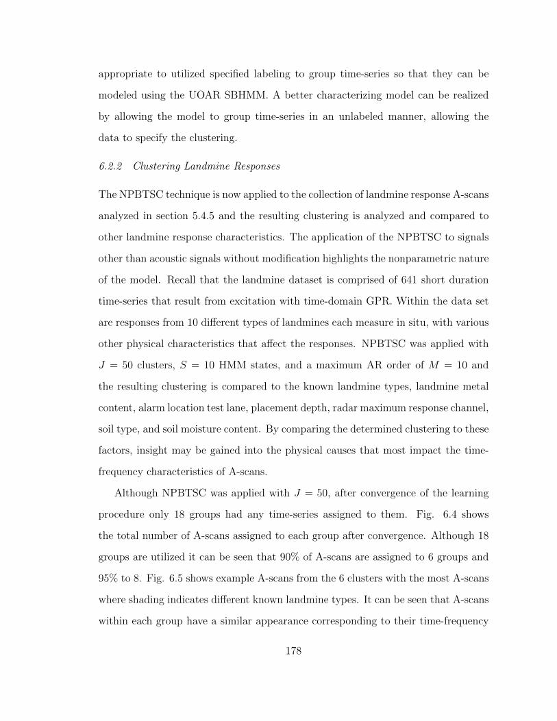
appropriate to utilized specified labeling to group time-series so that they can be

modeled using the UOAR SBHMM. A better characterizing model can be realized

by allowing the model to group time-series in an unlabeled manner, allowing the

data to specify the clustering.

6.2.2 Clustering Landmine Responses

The NPBTSC technique is now applied to the collection of landmine response A-scans

analyzed in section 5.4.5 and the resulting clustering is analyzed and compared to

other landmine response characteristics. The application of the NPBTSC to signals

other than acoustic signals without modification highlights the nonparametric nature

of the model. Recall that the landmine dataset is comprised of 641 short duration

time-series that result from excitation with time-domain GPR. Within the data set

are responses from 10 different types of landmines each measure in situ, with various

other physical characteristics that affect the responses. NPBTSC was applied with

J = 50 clusters, S = 10 HMM states, and a maximum AR order of M = 10 and

the resulting clustering is compared to the known landmine types, landmine metal

content, alarm location test lane, placement depth, radar maximum response channel,

soil type, and soil moisture content. By comparing the determined clustering to these

factors, insight may be gained into the physical causes that most impact the time-

frequency characteristics of A-scans.

Although NPBTSC was applied with J = 50, after convergence of the learning

procedure only 18 groups had any time-series assigned to them. Fig. 6.4 shows

the total number of A-scans assigned to each group after convergence. Although 18

groups are utilized it can be seen that 90% of A-scans are assigned to 6 groups and

95% to 8. Fig. 6.5 shows example A-scans from the 6 clusters with the most A-scans

where shading indicates different known landmine types. It can be seen that A-scans

within each group have a similar appearance corresponding to their time-frequency

178

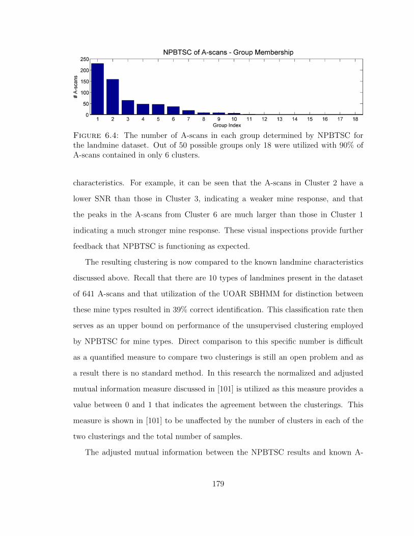
Figure 6.4: The number of A-scans in each group determined by NPBTSC forthe landmine dataset. Out of 50 possible groups only 18 were utilized with 90% ofA-scans contained in only 6 clusters.

characteristics. For example, it can be seen that the A-scans in Cluster 2 have a

lower SNR than those in Cluster 3, indicating a weaker mine response, and that

the peaks in the A-scans from Cluster 6 are much larger than those in Cluster 1

indicating a much stronger mine response. These visual inspections provide further

feedback that NPBTSC is functioning as expected.

The resulting clustering is now compared to the known landmine characteristics

discussed above. Recall that there are 10 types of landmines present in the dataset

of 641 A-scans and that utilization of the UOAR SBHMM for distinction between

these mine types resulted in 39% correct identification. This classification rate then

serves as an upper bound on performance of the unsupervised clustering employed

by NPBTSC for mine types. Direct comparison to this specific number is difficult

as a quantified measure to compare two clusterings is still an open problem and as

a result there is no standard method. In this research the normalized and adjusted

mutual information measure discussed in [101] is utilized as this measure provides a

value between 0 and 1 that indicates the agreement between the clusterings. This

measure is shown in [101] to be unaffected by the number of clusters in each of the

two clusterings and the total number of samples.

The adjusted mutual information between the NPBTSC results and known A-

179

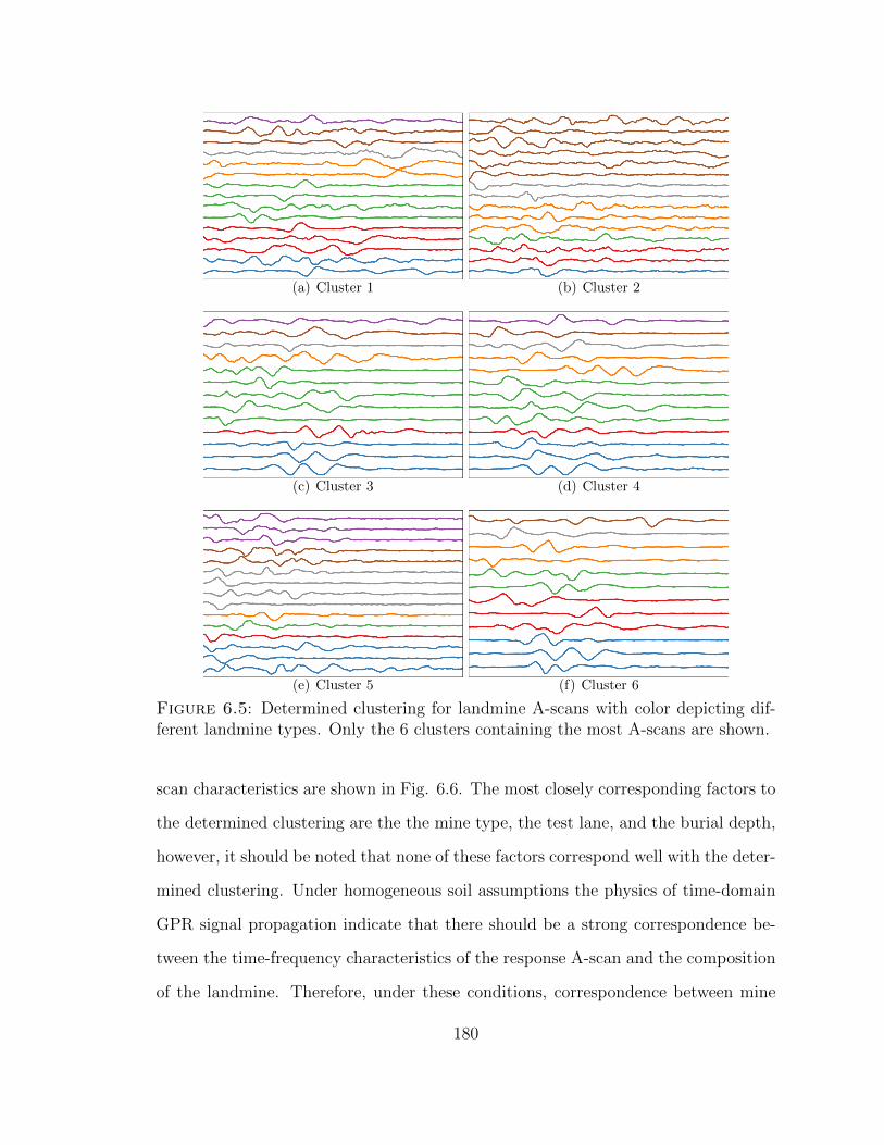
(a) Cluster 1 (b) Cluster 2

(c) Cluster 3 (d) Cluster 4

(e) Cluster 5 (f) Cluster 6

Figure 6.5: Determined clustering for landmine A-scans with color depicting dif-ferent landmine types. Only the 6 clusters containing the most A-scans are shown.

scan characteristics are shown in Fig. 6.6. The most closely corresponding factors to

the determined clustering are the the mine type, the test lane, and the burial depth,

however, it should be noted that none of these factors correspond well with the deter-

mined clustering. Under homogeneous soil assumptions the physics of time-domain

GPR signal propagation indicate that there should be a strong correspondence be-

tween the time-frequency characteristics of the response A-scan and the composition

of the landmine. Therefore, under these conditions, correspondence between mine

180

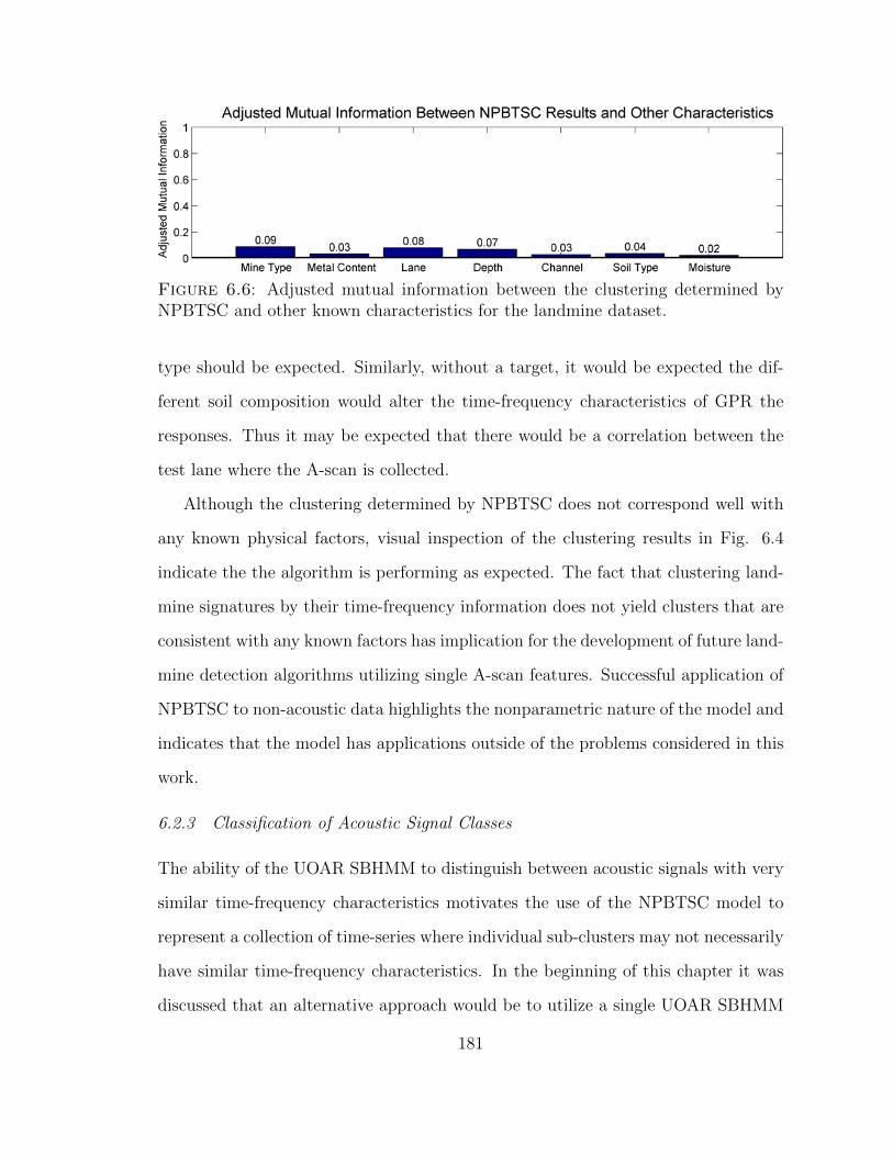
Figure 6.6: Adjusted mutual information between the clustering determined byNPBTSC and other known characteristics for the landmine dataset.

type should be expected. Similarly, without a target, it would be expected the dif-

ferent soil composition would alter the time-frequency characteristics of GPR the

responses. Thus it may be expected that there would be a correlation between the

test lane where the A-scan is collected.

Although the clustering determined by NPBTSC does not correspond well with

any known physical factors, visual inspection of the clustering results in Fig. 6.4

indicate the the algorithm is performing as expected. The fact that clustering land-

mine signatures by their time-frequency information does not yield clusters that are

consistent with any known factors has implication for the development of future land-

mine detection algorithms utilizing single A-scan features. Successful application of

NPBTSC to non-acoustic data highlights the nonparametric nature of the model and

indicates that the model has applications outside of the problems considered in this

work.

6.2.3 Classification of Acoustic Signal Classes

The ability of the UOAR SBHMM to distinguish between acoustic signals with very

similar time-frequency characteristics motivates the use of the NPBTSC model to

represent a collection of time-series where individual sub-clusters may not necessarily

have similar time-frequency characteristics. In the beginning of this chapter it was

discussed that an alternative approach would be to utilize a single UOAR SBHMM

181

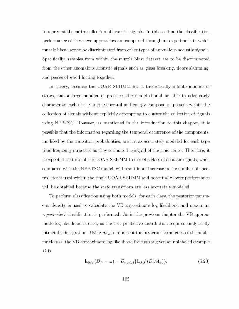
to represent the entire collection of acoustic signals. In this section, the classification

performance of these two approaches are compared through an experiment in which

muzzle blasts are to be discriminated from other types of anomalous acoustic signals.

Specifically, samples from within the muzzle blast dataset are to be discriminated

from the other anomalous acoustic signals such as glass breaking, doors slamming,

and pieces of wood hitting together.

In theory, because the UOAR SBHMM has a theoretically infinite number of

states, and a large number in practice, the model should be able to adequately

characterize each of the unique spectral and energy components present within the

collection of signals without explicitly attempting to cluster the collection of signals

using NPBTSC. However, as mentioned in the introduction to this chapter, it is

possible that the information regarding the temporal occurrence of the components,

modeled by the transition probabilities, are not as accurately modeled for each type

time-frequency structure as they estimated using all of the time-series. Therefore, it

is expected that use of the UOAR SBHMM to model a class of acoustic signals, when

compared with the NPBTSC model, will result in an increase in the number of spec-

tral states used within the single UOAR SBHMM and potentially lower performance

will be obtained because the state transitions are less accurately modeled.

To perform classification using both models, for each class, the posterior param-

eter density is used to calculate the VB approximate log likelihood and maximum

a posteriori classification is performed. As in the previous chapter the VB approx-

imate log likelihood is used, as the true predictive distribution requires analytically

intractable integration. UsingMω to represent the posterior parameters of the model

for class ω, the VB approximate log likelihood for class ω given an unlabeled example

D is

log q (D|c = ω) = Eq(Mω)log f (D|Mω). (6.23)

182

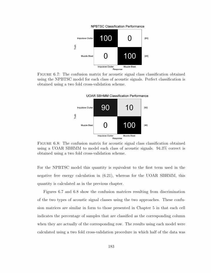
Figure 6.7: The confusion matrix for acoustic signal class classification obtainedusing the NPBTSC model for each class of acoustic signals. Perfect classification isobtained using a two fold cross-validation scheme.

Figure 6.8: The confusion matrix for acoustic signal class classification obtainedusing a UOAR SBHMM to model each class of acoustic signals. 94.3% correct isobtained using a two fold cross-validation scheme.

For the NPBTSC model this quantity is equivalent to the first term used in the

negative free energy calculation in (6.21), whereas for the UOAR SBHMM, this

quantity is calculated as in the previous chapter.

Figures 6.7 and 6.8 show the confusion matrices resulting from discrimination

of the two types of acoustic signal classes using the two approaches. These confu-

sion matrices are similar in form to those presented in Chapter 5 in that each cell

indicates the percentage of samples that are classified as the corresponding column

when they are actually of the corresponding row. The results using each model were

calculated using a two fold cross-validation procedure in which half of the data was

183

used to estimate parameters and the other half of the data was used to estimate per-

formance. This process was repeated so that each sample was used to evaluate the

performance without simultaneously being used to estimate the parameters. It can

be seen that use of NPBTSC to model each of the acoustic signal classes results in

perfect classification while use of an UOAR SBHMM for each class results in 93.4%

correct as 10% of non muzzle blast sounds are incorrectly identified as muzzle blasts.

The performance difference between the two approaches is congruent with the

expectation that more accurately modeling the transition between components can

result in performance improvements. Also congruent with expectation is the number

of HMM components utilized by each of the approaches. Although a maximum of S =

25 states were used for all SBHMMs under consideration, the SBHMMs within the

posterior NPBTSC models for each typically result in under 10 in use, while those in

the UOAR SBHMMs for each class resulting in nearly all of the S = 25 states in use.

The clusterings determined by NPBTSC for the muzzle blast class are very similar to

those observed in Section 6.2.1. While the samples within the non-muzzle blast class

yield clustering results more congruent with the clustering results of the Arisaka

Type 38A rifle, in that each of the labeled classes are typically partitioned into

several smaller groups that have more similar time-frequency structures. Therefore,

the NPBTSC model results in more HMMs with fewer states while a single UOAR

SBHMM uses only a single HMM by definition but this HMM is required to have

more states to model all of the unique components of the dataset.

On this limited dataset it can be seen that there is a benefit to utilizing the

NPBTSC model for classification of acoustic signal classes that are comprised of

time-series with potentially different time-frequency characteristics. However, to

draw more definitive conclusions regarding the expected performance for a particular

application the two approaches would need to be compared on more comprehensive

datasets representative of the problem under consideration. It is not anticipated that

184

use of NPBTSC would result in perfect classification in practice for every possible

problem, however, it appears that the model is capable of characterizing a collection

of time-series in a completely nonparametric manner and therefore provides a means

to perform classification between classes. Although similar performance is obtained

by using a single UOAR SBHMM for each class, there are more advantages to the use

of the NPBTSC model other than the slight performance improvement obtained by

more accurately modeling the transition probabilities within each time-series type.

Not only is the model more representative of physical interpretation of the problem

it also offers advantages when performing recursive Bayesian estimation to adapt the

model of an acoustic signal class when additional information is received.

6.3 Dynamic Updating of Acoustic Signal Class Models

Throughout this work Bayesian inference, specifically the VB method, has been used

to determine the posterior density for the parameters of models for acoustic signals.

In Chapter 3, non-stationary AR models were used to perform adaptive modeling

of acoustic background signals to enable detection of anomalous acoustic signals. In

subsequent chapters the VB method has been used to develop parameter inference

procedures for nonparametric models to distinguish between anomalous acoustic sig-

nals. The NPBTSC model developed in this chapter serves as a model that can

be used to discriminate between classes of acoustic signals and enable detection of

specific events of interest to a particular acoustic surveillance system. The nature of

the NPBTSC model, specifically its parameterized posterior density, also enables a

principled manner in which the model for acoustic signal classes can be updated as

new data is received.

Chapter 1 discussed an example of a vehicle mounted gunshot detection system

which travels to new locations and encounters anomalous acoustic signals that have

time-frequency characteristics that are not characterized by the signal models already

185

within the system. As a result, poor classification results are obtained for these

new signals. A similar scenario may arise in a stationary gunshot detection system

mounted on a street pole. Perhaps a car belonging to a person that lives in a nearby

building has recently started to backfire occasionally. Suppose also that the time-

frequency of the car back-fire signal is such that these events are misidentified as

gunfire. As a result, police resources are wasted as officers are contacted to respond

to the event. If these events are appropriately logged, the use of the NPBTSC to

perform discrimination enables the model to incorporate this new information, as

the NPBTSC model for the class of non-muzzle blast acoustic signals can be updated

to include a the car backfire signals. Although this type of updating requires input,

i.e. a practitioner to inform the system of the correct acoustic signal class of the

samples to use for updating, it does not require the full collection of data that was

used to train the entire model. In real-world systems this type of feedback is often

available and this learning process can be considered a form of operator in the loop

processing, in which the analyst has an ability to influence the future behavior of the

system.

It was discussed in Chapter 2 that conjugate priors offer a method to perform

analytically tractable recursive Bayesian estimation, wherein the posterior density at

time t can be used as the prior density at time t+ 1. Recursive Bayesian estimation

provides a method by which all previously observed data can be encapsulated in the

posterior distribution and therefore when new data is received, a model representing

all data can be derived using only the newly received data and the previous posterior

density, eliminating the need to retain all previous data. For problems such as

acoustic surveillance where the dataset used to train the model may be quite large,

recursive Bayesian estimation provides a means of performing algorithmic adaptation

in fielded systems that do not have the resources to store the large training dataset.

In this section, recursive Bayesian updating of the NPBTSC model is examined

186

within the context of an acoustic sensing task in which feedback regarding misidenti-

fied samples is provided by an analyst. In theory, recursive Bayesian updating of the

NPBTSC model should allow for the model to determine when it is necessary to in-

corporate a new time-series type into the model. Therefore, continuing the example

above, if the NPBTSC model for non-muzzle blasts signals is updated using examples

of car backfire, a new UOAR SBHMM should be incorporated into the new posterior

NPBTSC model to model these samples. However, due to the nature of approximate

Bayesian inference for models with hidden variables, there are computational and

inference algorithm issues that must be considered to ensure the algorithm provides

robust performance. Therefore, prior to consideration of the NPBTSC model these

issues are discussed in general terms.

6.3.1 Recursive Variational Bayesian Inference with Hidden Variables

The VB method optimizes the parameters of an approximate posterior density for

a set of parameters q (θ) to minimize the KLD between this approximate posterior

density and the true unknown unattainable posterior density. In Chapter 2 it was

discussed how minimization of this KLD is equivalent to maximizing the negative

free energy

F (q (θ)) = Eq(θ)log f (D|θ) −KL (q (θ) ||f (θ)) . (6.24)

In Chapter 4 it was discussed how the two terms of the negative free energy balance

the fit of the model (the first term), and the complexity of the model (the second

term), and that this optimization criterion leads the VB method to perform auto-

mated model order selection. This interpretation of the VB method also provides

insight into the expected behavior of recursive Bayesian inference in the presence of

hidden variables.

Recall that when hidden variables are present within a model, such as the group

membership variables in the NPBTSC model zi, the learning algorithm resulting

187

from the VB method can be interpreted as a two stage approach in which first

the hidden parameters are estimated and then, using the current estimates of these

hidden parameters, the other parameters in the model are estimated. This process

repeats and at each iteration the accuracy of the hidden variables (only truly measur-

able in example problems when the underlying hidden variables is known) increases.

Through this iterative process the entire dataset is used to jointly estimate the col-

lection of hidden variables more accurately. In the presence of limited data however,

the quality of the estimated hidden parameters is restricted by the lack of data.

The recursive Bayesian updating of the NPBTSC model of focus to this work

can be discussed in more general terms by considering recursive variational Bayesian

updating of a DP mixture model of data x and component parameters θ∗i for i ∈

[1, 2, . . . , J ] where J is a very large number. Suppose that the posterior density for

this mixture model has been determined from some initial training dataset D using

th VB methodology described in Chapter 4 which yields a posterior density q1 (Ω)

where Ω represents all of the parameters of the model. Within this posterior mixture

model only a few of the J mixture components, J∗, have posterior densities that

are different from their prior densities, thus illustrating the model order selection

property of DP mixtures.

Now suppose that new data Dnew is received and recursive Bayesian updating is to

be applied to form a new posterior density posterior q2 (Ω). The hidden parameters

that must be estimated for this new data are the component memberships for each

point. First consider the case when Dnew is comprised of a only single observation

xnew and therefore, the only hidden parameter is znew. There are then two possibilities

for the hidden parameter znew. A value of znew ∈ [1, 2, . . . , J∗] would indicate the

the point xnew originates from the one of the already characterized components of

the mixture model. Alternatively a value of znew = J∗+ 1 would indicate that point

xnew comes from a new component within the model. The more appropriate choice

188

between these two depends on several factors but can be discussed through analysis

of the negative free energy.

The more appropriate of the two possible assignments of znew is the assignment

that yields the higher negative free energy, as is true with any two initializations of

a VB learning procedure [46]. The negative free energy for the recursive variational

Bayesian update for this new point can be written as

F (q (Ω1)) = Eq2(Ω)log f (D|Ω) −KL (q2 (Ω) ||q1 (Ω))

=J∑i=1

log qΩ2 (znew = i) + Eq2(Ω)log f (xnew|θ∗i )

−J∑i=1

KL (q2 (θ∗i ) |q1 (θ∗i ))

−J∑i=1

KL (q2 (ρk) |q1 (ρk)) (6.25)

where the prior density has been replaced by q1 (Ω) and definitions of the negative

free energy for a DP mixture model have been used. Note that the expected values

in (6.25) and in the remainder of this section are taken with respect to q2 (Ω). The

negative free energy is comprised of three terms, the average log-likelihood, the KLD

of the component densities, and the KLD of the stick-breaking densities. For the

analysis that follows, the stick-breaking parameters are omitted from discussion as

the effect of these terms is negligible. If the new data point is determined to originate

from one of the already characterized components in the mixture, the first term of

the negative free energy, the average variational log-likelihood, will be the primary

deciding force determining the quantity. This is because the posterior density for each

component in the mixture is derived from several samples and therefore, it is unlikely

that updating any component using a single sample will result in a significant change

in the KLD from the new posterior to the old posterior for the assigned component.

189

Therefore, because only J∗ of the components have posterior densities that differ

from the prior, each term of the summation within the second term of the negative

free energy for i > J∗ is equal to zero, and from 1 ≤ i ≤ J∗ these terms are very

small. However, if the sample is assigned to begin a new component in the mixture,

znew = J∗ + 1, the average log-likelihood may be fairly high. However, in this case

the KLD term corresponding to the J∗ + 1 component will also be very large, as

previously this component had a posterior density equal to the prior and now the

posterior density has changed significantly.

As a simplifying example, again consider the effects of the stick-breaking param-

eters to be negligible and consider that the posterior density for the hidden variable

has a value of exactly 1 for component k. Consider two cases for the value of k,

assignment to an existing component, 1 ≤ k ≤ J∗, and assignment to a new com-

ponent k = J∗ + 1. For these two cases, the negative free energy will be compared.

For the case of assignment to an existing component, the negative free energy can

be approximated as

Fexisting ≈ Elog f (xnew|θ∗k) −KL (q2 (θ∗k) |q1 (θ∗k))

≈ Elog f (xnew|θ∗k) (6.26)

where it is assumed that the change in the posterior density of the kth component

from the influence of a single data point results in a negligible KLD. For the al-

ternative case, assignment to a new component, the negative free energy can be

approximated as

Fnew ≈ Elog f (xnew|θ∗k) −KL (q2 (θ∗k) |f (θ∗k)) (6.27)

The larger of these two negative free energies will determine whether assignment

to a new component or to an existing component is more appropriate. Although

this is only a simplifying example, it illustrates how a new mixture component can

be inferred from newly incoming data through recursive Bayesian updating in DP

190

mixtures. The decision to assign the new data point to create a new component is

determined by the prior parameters of the model in (6.27) and the likelihood of the

data in existing components (6.26).

Now consider that there are multiple samples in Dnew all originating from an as

yet uncharacterized component of the mixture model. In this case, comparison of

the above cases is similar except that the KLD term of (6.27) may not be as strong

of a penalty term as the the difference in the average log likelihood that is obtained

by assigning both samples to an existing cluster. Therefore, it may be deemed more

appropriate to assign both samples to a new cluster. As a result of this analysis it can

be seen that in the presence of hidden variables, it is advantageous for the learning

procedure to have multiple examples from the new component to ensure that a new

component is inferred. For example, suppose that there are now two samples in

Dnew. If only one of the samples is used to update the posterior density, then a new

component would not be created and the density of an existing component would be

modified. If the second sample is then used to update the new posterior density, this

component may also not be assigned to a new component. However, if both samples

are used simultaneously to update the posterior density, it is possible that both data

points would be assigned to a new component.

In conclusion, recursive Bayesian estimation of DP mixtures is a tractable task

that requires comparison of the negative free energy obtained through assignment

of the sample to a previously empty component within the mixture and assignment

of the sample to an existing component in the mixture. The ability of the model to

correctly assign new data points to new components is linked strongly to the average

log likelihood of the data with the existing components and the prior density for

the component parameters. Greater assignment accuracy can be obtained by using

multiple observations simultaneously when performing recursive Bayesian updating.

Therefore, performance of a system utilizing recursive Bayesian updating of a model

191

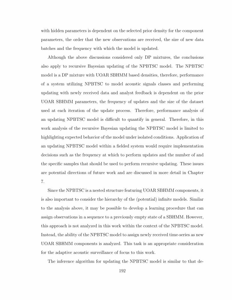
with hidden parameters is dependent on the selected prior density for the component

parameters, the order that the new observations are received, the size of new data

batches and the frequency with which the model is updated.

Although the above discussions considered only DP mixtures, the conclusions

also apply to recursive Bayesian updating of the NPBTSC model. The NPBTSC

model is a DP mixture with UOAR SBHMM based densities, therefore, performance

of a system utilizing NPBTSC to model acoustic signals classes and performing

updating with newly received data and analyst feedback is dependent on the prior

UOAR SBHMM parameters, the frequency of updates and the size of the dataset

used at each iteration of the update process. Therefore, performance analysis of

an updating NPBTSC model is difficult to quantify in general. Therefore, in this

work analysis of the recursive Bayesian updating the NPBTSC model is limited to

highlighting expected behavior of the model under isolated conditions. Application of

an updating NPBTSC model within a fielded system would require implementation

decisions such as the frequency at which to perform updates and the number of and

the specific samples that should be used to perform recursive updating. These issues

are potential directions of future work and are discussed in more detail in Chapter

7.

Since the NPBTSC is a nested structure featuring UOAR SBHMM components, it

is also important to consider the hierarchy of the (potential) infinite models. Similar

to the analysis above, it may be possible to develop a learning procedure that can

assign observations in a sequence to a previously empty state of a SBHMM. However,

this approach is not analyzed in this work within the context of the NPBTSC model.

Instead, the ability of the NPBTSC model to assign newly received time-series as new

UOAR SBHMM components is analyzed. This task is an appropriate consideration

for the adaptive acoustic surveillance of focus to this work.

The inference algorithm for updating the NPBTSC model is similar to that de-

192

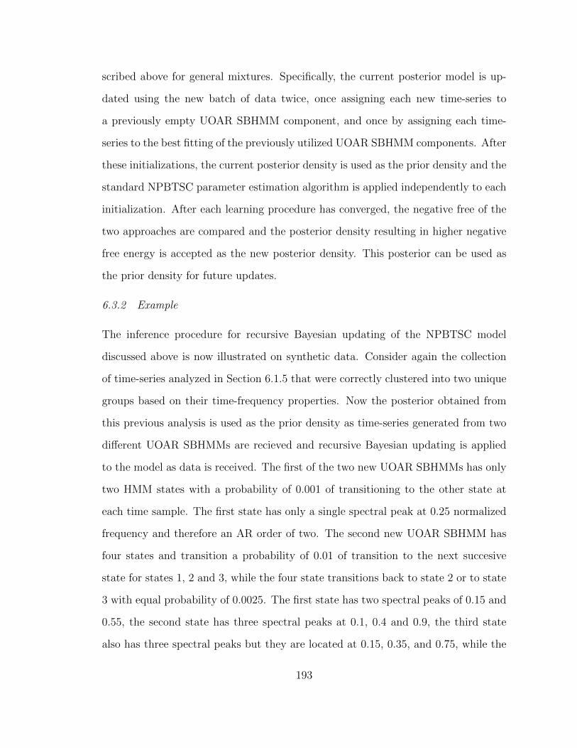
scribed above for general mixtures. Specifically, the current posterior model is up-

dated using the new batch of data twice, once assigning each new time-series to

a previously empty UOAR SBHMM component, and once by assigning each time-

series to the best fitting of the previously utilized UOAR SBHMM components. After

these initializations, the current posterior density is used as the prior density and the

standard NPBTSC parameter estimation algorithm is applied independently to each

initialization. After each learning procedure has converged, the negative free of the

two approaches are compared and the posterior density resulting in higher negative

free energy is accepted as the new posterior density. This posterior can be used as

the prior density for future updates.

6.3.2 Example

The inference procedure for recursive Bayesian updating of the NPBTSC model

discussed above is now illustrated on synthetic data. Consider again the collection

of time-series analyzed in Section 6.1.5 that were correctly clustered into two unique

groups based on their time-frequency properties. Now the posterior obtained from

this previous analysis is used as the prior density as time-series generated from two

different UOAR SBHMMs are recieved and recursive Bayesian updating is applied

to the model as data is received. The first of the two new UOAR SBHMMs has only

two HMM states with a probability of 0.001 of transitioning to the other state at

each time sample. The first state has only a single spectral peak at 0.25 normalized

frequency and therefore an AR order of two. The second new UOAR SBHMM has

four states and transition a probability of 0.01 of transition to the next succesive

state for states 1, 2 and 3, while the four state transitions back to state 2 or to state

3 with equal probability of 0.0025. The first state has two spectral peaks of 0.15 and

0.55, the second state has three spectral peaks at 0.1, 0.4 and 0.9, the third state

also has three spectral peaks but they are located at 0.15, 0.35, and 0.75, while the

193

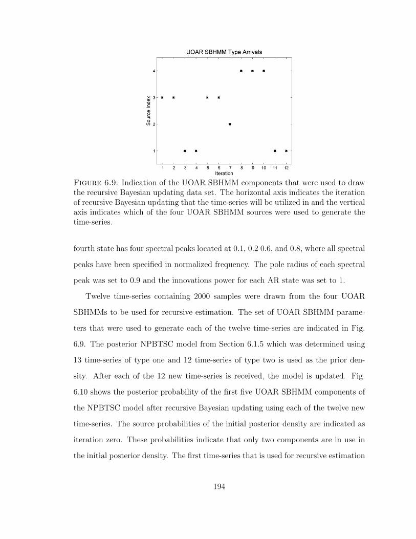
Figure 6.9: Indication of the UOAR SBHMM components that were used to drawthe recursive Bayesian updating data set. The horizontal axis indicates the iterationof recursive Bayesian updating that the time-series will be utilized in and the verticalaxis indicates which of the four UOAR SBHMM sources were used to generate thetime-series.

fourth state has four spectral peaks located at 0.1, 0.2 0.6, and 0.8, where all spectral

peaks have been specified in normalized frequency. The pole radius of each spectral

peak was set to 0.9 and the innovations power for each AR state was set to 1.

Twelve time-series containing 2000 samples were drawn from the four UOAR

SBHMMs to be used for recursive estimation. The set of UOAR SBHMM parame-

ters that were used to generate each of the twelve time-series are indicated in Fig.

6.9. The posterior NPBTSC model from Section 6.1.5 which was determined using

13 time-series of type one and 12 time-series of type two is used as the prior den-

sity. After each of the 12 new time-series is received, the model is updated. Fig.

6.10 shows the posterior probability of the first five UOAR SBHMM components of

the NPBTSC model after recursive Bayesian updating using each of the twelve new

time-series. The source probabilities of the initial posterior density are indicated as

iteration zero. These probabilities indicate that only two components are in use in

the initial posterior density. The first time-series that is used for recursive estimation

194

Figure 6.10: Component probabilities after each iteration of recursive Bayesianupdating of the NPBTSC model. It can be seen that new time-series types areinferred when they are indicated to arrive in Fig. 6.9. At these points previouslyvery small (zero) components probabilities increase indicating the assignment of thetime-series into a new NPBTSC component. This occurs most notably at iteration1 and 8.

(a) UOAR SBHMM 3 (b) UOAR SBHMM 4

Figure 6.11: Illustration of the estimated UOAR SBHMM parameters for the newlydetermined NPBSTC components

is from the third time-series type. The inference algorithm correctly determines that

this time-series type is better modeled using a new UOAR SBHMM and therefore

the time-series is assigned to the third component. Iterations 2 through 7 use time-

series from the first three UOAR SBHMM components that are already represented

in the model. The inference procedure correctly determines the correct component

for each of these time-series and after each it can be seen that the component prob-

ability for the assigned component increases and the other components decrease. A

195

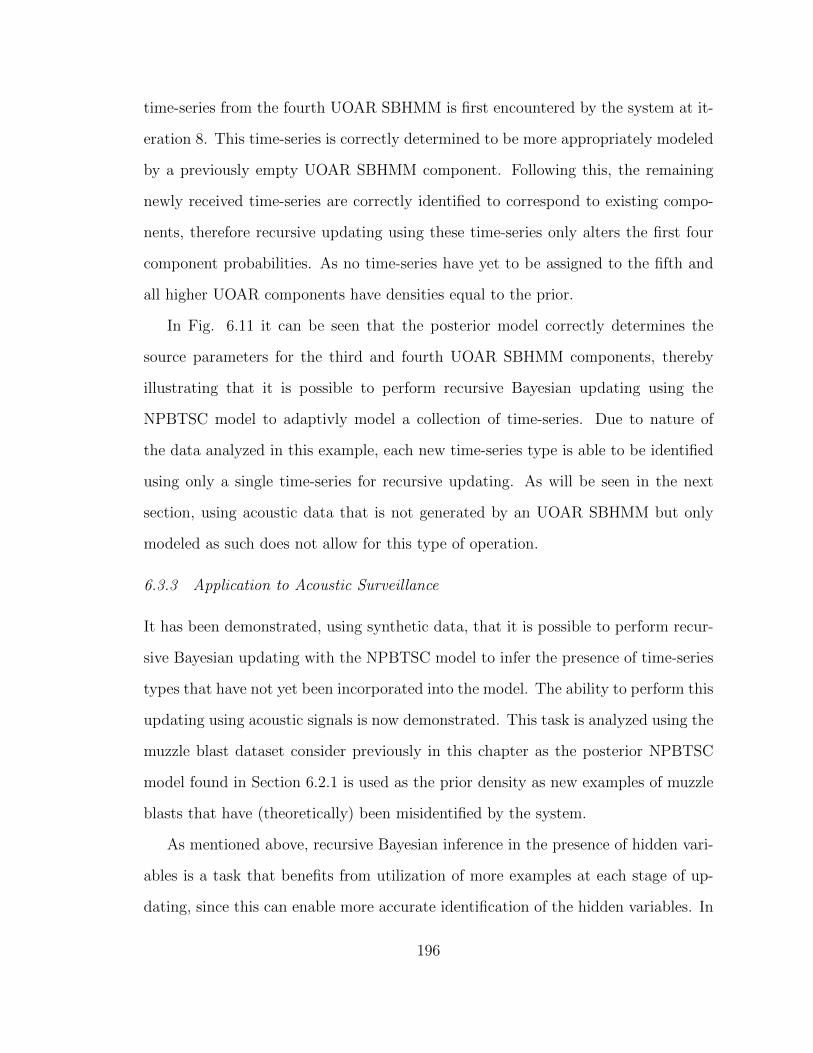
time-series from the fourth UOAR SBHMM is first encountered by the system at it-

eration 8. This time-series is correctly determined to be more appropriately modeled

by a previously empty UOAR SBHMM component. Following this, the remaining

newly received time-series are correctly identified to correspond to existing compo-

nents, therefore recursive updating using these time-series only alters the first four

component probabilities. As no time-series have yet to be assigned to the fifth and

all higher UOAR components have densities equal to the prior.

In Fig. 6.11 it can be seen that the posterior model correctly determines the

source parameters for the third and fourth UOAR SBHMM components, thereby

illustrating that it is possible to perform recursive Bayesian updating using the

NPBTSC model to adaptivly model a collection of time-series. Due to nature of

the data analyzed in this example, each new time-series type is able to be identified

using only a single time-series for recursive updating. As will be seen in the next

section, using acoustic data that is not generated by an UOAR SBHMM but only

modeled as such does not allow for this type of operation.

6.3.3 Application to Acoustic Surveillance

It has been demonstrated, using synthetic data, that it is possible to perform recur-

sive Bayesian updating with the NPBTSC model to infer the presence of time-series

types that have not yet been incorporated into the model. The ability to perform this

updating using acoustic signals is now demonstrated. This task is analyzed using the

muzzle blast dataset consider previously in this chapter as the posterior NPBTSC

model found in Section 6.2.1 is used as the prior density as new examples of muzzle

blasts that have (theoretically) been misidentified by the system.

As mentioned above, recursive Bayesian inference in the presence of hidden vari-

ables is a task that benefits from utilization of more examples at each stage of up-

dating, since this can enable more accurate identification of the hidden variables. In

196

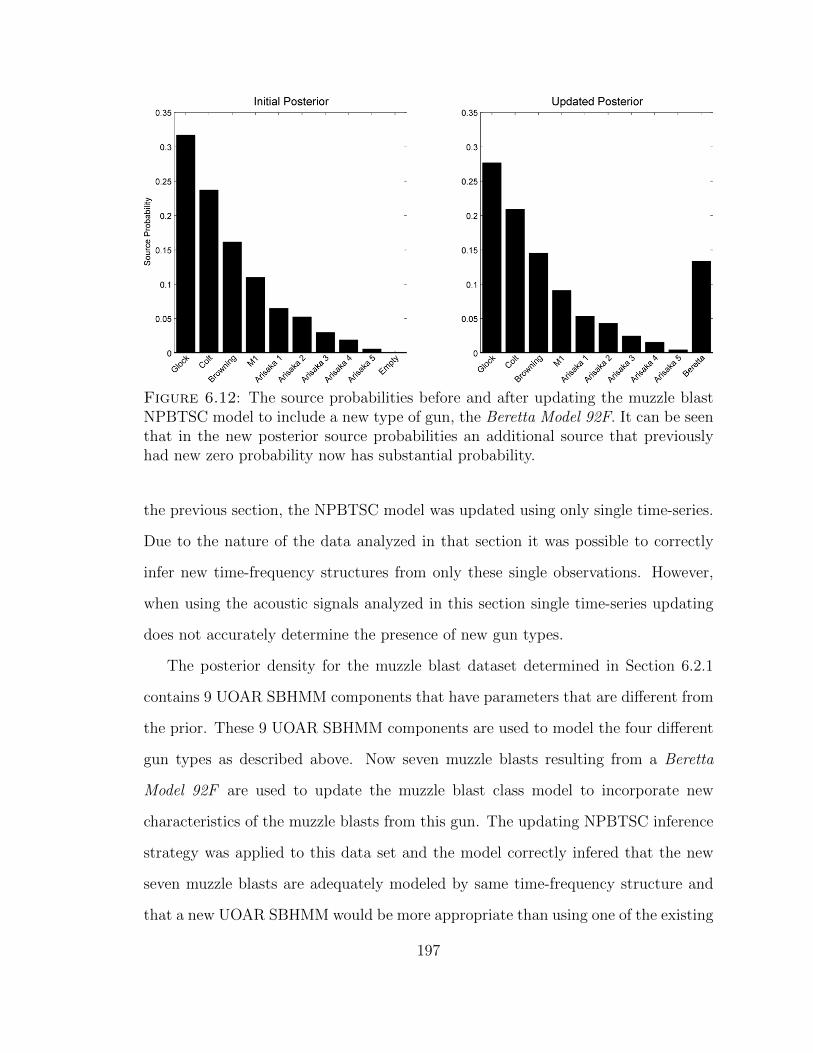
Figure 6.12: The source probabilities before and after updating the muzzle blastNPBTSC model to include a new type of gun, the Beretta Model 92F. It can be seenthat in the new posterior source probabilities an additional source that previouslyhad new zero probability now has substantial probability.

the previous section, the NPBTSC model was updated using only single time-series.

Due to the nature of the data analyzed in that section it was possible to correctly

infer new time-frequency structures from only these single observations. However,

when using the acoustic signals analyzed in this section single time-series updating

does not accurately determine the presence of new gun types.

The posterior density for the muzzle blast dataset determined in Section 6.2.1

contains 9 UOAR SBHMM components that have parameters that are different from

the prior. These 9 UOAR SBHMM components are used to model the four different

gun types as described above. Now seven muzzle blasts resulting from a Beretta

Model 92F are used to update the muzzle blast class model to incorporate new

characteristics of the muzzle blasts from this gun. The updating NPBTSC inference

strategy was applied to this data set and the model correctly infered that the new

seven muzzle blasts are adequately modeled by same time-frequency structure and

that a new UOAR SBHMM would be more appropriate than using one of the existing

197

UOAR SBHMMs in the model. The source probabilities from the initial posterior

model from Section 6.2.1 and the source probabilities from the new posterior model

with an inferred additional source are shown in Fig. 6.12. It can be seen that the

component probabilities have been adjusted to incorporate a new UOAR SBHMM

into the model and give this component positive probability.

The above demonstrates that it is possible to update the NPBTSC model using

multiple time-series and that from this collection of time-series new time-frequency

types can be identified and modeled using a previously un-utilized UOAR SBHMM

component within the model. However, the number of time-series required to update

the model may vary with the model used. In the previous section single time-series

were used to infer the presence of a new time-series type. However, performing this

method with the muzzle blast data set using a single example from of the Beretta

Model 92F considered above, does not result in inference of a new type. This is

because the single muzzle blast has an average log likelihood with one of the existing

clusters that is not substantially lower than the average log likelihood obtained from

a UOAR SBHMM trained using the single muzzle blast. Therefore, the total model

negative free energy for the initialization that assigns the single muzzle blast to one

of the existing UOAR SBHMMs is higher. However, if a single new muzzle blast has

substantially different time-frequency characteristics than those modeled by any of

the existing UOAR SBHMMs a new type can be inferred.

Now a single acoustic signal resulting from an LRM Missile Launcher is incor-

porated into the muzzle blast model. The updating inference algorithm for the

NPBTSC model is applied to the posterior model from Section 6.2.1. The infer-

ence procedure correctly determines that the signal has dramatically different time-

frequency characteristics than any of those already model by the UOAR SBHMMs

in the model and therefore a new UOAR SBHMM should be estimated using only

this example. An illustration of the UOAR SBHMM parameters estimated from this

198

Figure 6.13: Illustration of the UOAR SBHMM parameters inferred from a sin-gle example of a missile launcher. It can be seen that this example has dramaticallydifferent time-frequency characteristics compared to other muzzle blasts already con-tained in the model.

acoustic signal are shown in Fig. 6.13. This figure is analogous to those seen previ-

ously and it can be seen that this example has dramatically different time-frequency

characteristics compared to the muzzle blasts already characterized by the modeled

and illustrated in Fig. 5.2.

This illustrates that it is possible to correctly infer the presence of a new time-

frequency structure from a single acoustic signal provided that the signature has

significantly different time-frequency characteristics. In practice, however, it is not

possible to know in advance whether the signal to be used to update the model will

yield a new time-series type or if a new time-series type would be necessary even if

additional similar acoustic signals were available. Therefore, although it is possible

to appropriately infer the presence of a time-frequency structure from only a single

example, in practice it would be better to use more examples to update the model

to enable more accurate identification of the hidden variables.

6.4 Conclusions

This chapter has developed and analyzed a nonparametric Bayesian model for classes

of acoustic signals that can be updated through Bayesian inference to add knowledge

199

of new types of signals within each class without the need to retain the data initially

used to train the model. The model is realized by considering a DP mixture of the

UOAR SBHMM sources developed and analyzed in the previous two chapters. It was

demonstrated that parameter inference for this model performs an automatic clus-

tering of the time-series and the model was thus named the nonparametric Bayesian

time-series cluster (NPBTSC) model.

It was demonstrated that the NPBTSC model can be used to perform nonpara-

metric clustering of time-series data using synthetic data as well as acoustic sig-

nals, and landmine responses from time-domain ground penetrating radar data. The

model is able to accurately cluster time-series that have similar time-frequency char-

acteristics while simultaneously modeling these time-frequency characteristics and

determining the number of unique time-frequency types. The ability to correctly clus-

ter time-series with similar time-frequency characteristics was demonstrated within

each application.

The NPBTSC model was developed to serve as a parameterized model that can

represent a collection of acoustic signal models that may have differing time-frequency

characteristics and provide a means to perform classification between collections of

signals described only by abstract designations such as “muzzle blasts” or “sounds

indicative of a security breach”. The ability to distinguish between classes such as

these was demonstrated in an acoustic surveillance context wherein muzzle-blasts

were accurately distinguished from other anomalous sounds. Modeling each class us-

ing NPBTSC enables better classification performance than utilizing a single UOAR

SBHMM to model each class since the temporal relationship between the spectral

and energy characteristics are more accurately modeled, in the NPBTSC model.

Utilizing NPBTSC to model each class also enables algorithmic adaptation through

recursive Bayesian updating.

The use of Bayesian inference throughout this work has been motivated by the

200

desire to create an acoustic sensing algorithm that is capable of adapting to changing

environmental and operational conditions in a principled manner. In this chapter it

was demonstrated that the NPBTSC model for a class of signals can be updated using

a collection of signals that may have been misidentified by the acoustic surveillance

system to modify the model to more accurately characterize these signals. It was

demonstrated that because NPBTSC generates a parameterized posterior density,

recursive Bayesian updating can be applied in a computationally tractable manner

to accomplish this task. An inference algorithm was developed that is capable of

identifying and incorporating into the model new time-frequency structures that had

not previously been characterized by the model. It was illustrated that new types

of muzzle blasts can be identified and modeled in a NPBTSC model that already

characterizes other types of muzzle blasts, without the need to utilize previously seen

training data. Although there are implementation issues that must be considered to

utilize algorithmic adaptation in a fielded system, the NPBTSC provides a principled

manner to accomplish algorithmic adaptation in an acoustic surveillance system.

The NPBTSC model serves as the final component of the acoustic surveillance

framework proposed in this research. It can be used to characterize a class of acous-

tic signals that may not have common time-frequency characteristics, and can be

adapted, through Bayesian methodology, to characterize previously misidentified

signals if deemed necessary. In the final chapter the proposed acoustic surveillance

framework is summarized and the conclusions made in this work are discussed along

with possible directions of future work.

201

7

Conclusions and Future Work

7.1 Summary of Completed Work

This research has developed a framework for adaptive acoustic surveillance that uti-

lizes nonparametric Bayesian methods to create algorithms that are independent

of the specific signals under consideration. The use of the variational Bayes (VB)

method to perform approximate Bayesian inference for the parameters of the pro-

posed models results in posterior densities of the same functional form as the prior

densities [46], thereby facilitating computationally tractable methods for recursive

Bayesian inference that serve as principled methods to adapt the algorithm to chang-

ing environmental or operational conditions.

The proposed framework for acoustic surveillance is a two stage approach in which

first, anomalous signals are detected within ever-present background acoustic signals,

and second, anomalous signals of interest are distinguished from other anomalous

signals. This two stage approach separates the tasks of characterizing the background

signals and characterizing the signals of interest and other anomalous sounds and is

a fundamental difference between the proposed approach and previous approaches

202

to algorithms applicable to acoustic surveillance [12, 13, 14, 15, 16, 17]. Separating

these two tasks allows for non-stationary modeling of the background signals as a

means to perform detection without using knowledge of the specific signals of interest,

analyzed in Chapter 3, and maintaining a stationary model for the signals of interest,

analyzed in Chapters 4-6.

In Chapter 3, an algorithm to accomplish the proposed first stage of processing is

developed and analyzed. The proposed technique is based on non-stationary autore-

gressive (AR) modeling of background signals and detecting deviations in this model

to infer the presence of anomalous signals. AR models are a generative statistical

process that are capable of characterizing the spectral and energy characteristics of

time-series data while the use of non-stationary modeling enables the background sig-

nal model to track the time-varying statistical nature of the signals. Both maximum

likelihood (ML) and Bayesian inference procedures for non-stationary AR models

were analyzed in the context of a muzzle blast detection experiment and it was de-

termined that Bayesian non-stationary AR (BNSAR) modeling is able to provide

superior performance in the majority of the conditions tested. The resulting algo-

rithm for BNSAR modeling is computationally similar to the resulting maximum

likelihood algorithm, least mean squares (LMS), but is able to more accurately cal-

culate instantaneous estimates of both the AR weights and the innovations power of

the AR model without additional ad hoc processing.

After anomalous signals are detected using BNSAR modeling in the first stage

of processing, anomalous signals of interest must be discriminated from other pos-

sible anomalous signals in the second stage of processing. Statistical models that

can be used to perform classification of anomalous acoustic signals were developed

and analyzed in Chapters 4-6 of this work. A primary motivating factor behind the

methodology employed to develop these models was the desire to remain indepen-

dent of particular signals of interest and to create algorithms that enable principled

203

methods to perform algorithm adaptation. A motivating example throughout this

work has been that of a mobile gunshot detection system, that travels and encounters

anomalous signals that are as yet uncharacterized by the system. As a result, the

uncharacterized signals may be incorrectly determined to be gunshots or rejected as

another anomalous sound. The classification algorithms developed in this research

achieved both of these goals, application independence and adaptability, through the

use of statistical models that make use of nonparametric Bayesian methods and have

parameters inferred using the VB method.

In Chapter 4 a nonparametric model capable of characterizing the time-frequency

information of time-series were developed and analyzed. The model operates directly

on the time-domain data instead of transforming the data into a set or sequence

of characterizing features as is often done when processing acoustic signals (e.g.

[29, 102]), and by doing so the need to select or design these features on an appli-

cation specific basis is eliminated. As in Chapter 3, AR models were employed to

characterize the spectral and energy characteristics of the data, however, to elim-

inate dependence of the model on a selected AR order, and thus allow the model

to automatically infer the spectral complexity, the uncertain-order AR (UOAR) was

formalized and analyzed. It was determined that UOAR models can accurately de-

termine the correct AR order within synthetic data more accurately than automatic

relevance determination, and therefore UOAR models are an appropriate choice for

a statistical model to characterize spectral and energy characteristics while simulta-

neously inferring the spectral complexity.

The ability of UOAR models to characterize spectral and energy characteristics of

time-series data without the need to specify the AR order is exploited in the statistical

models developed in the remainder of Chapter 4 and in Chapter 5 where a collection

of UOAR models are used within larger statistical models to characterize the time-

frequency information of signals. In the latter part of Chapter 4 a Dirichlet process

204

(DP) mixture model was used to characterize time-series data with changing spectral

and energy characteristics. Statistical methods utilizing DP priors yield statistical

learning algorithms that automatically determine the appropriate number discrete

components within a statistical model. A VB learning algorithm was developed for

the parameters of a DP mixture of UOAR components and it was determined that

VB inference for this model is able to determine the correct number of components

within the mixture as well as the correct AR order of each component with accuracy

similar to that obtained when using computationally expensive Markov chain Monte

Carlo (MCMC) inference. Finally, it was demonstrated that the use of statistical

models featuring automated model selection are able to perform comparably to the

best performance obtained by performing a computationally expensive search over

possible model orders. This was demonstrated through an acoustic surveillance task

of focus to this work, as a DP mixture of UOAR components was used to model

classes of acoustic signals similar to those that are to be distinguished in the second

stage of the proposed acoustic surveillance framework.

In Chapter 5 the DP mixture of UOAR components was adapted to include

a model for not only the frequency of occurrence but also the temporal structure

of the occurrence of the UOAR components. This was done by incorpoarting the

UOAR model as the state density within a hidden Markov model (HMM). It was

discussed that a prior structure for a HMM that permits automatic determination

of the appropriate number of states and allows for use of the VB method is closely

related to the DP and is known as the SBHMM [23]. A VB inference procedure for the

UOAR SBHMM was then developed and it was also demonstrated that the algorithm

is capable of determining not only the appropriate number of unique spectral and

energy components within a signal but also the spectral complexity within each of

these states. It was demonstrated that the time-frequency information characterized

by the UOAR SBHMM can be interpreted in a manner similar to the short-time

205

Fourier transform. Further, because the UOAR SBHMM is a generative statistical

model operating directly on the time-series data, it is possible to use the model to

generate synthetic data with time-frequency properties similar to those used to infer

the parameters of the model. Finally, it was demonstrated that the UOAR SBHMM

can be used to perform discrimination between different types of acoustic signals

and that the UOAR SBHMM provides superior performance to standard feature

based classification approaches for acoustic signal discrimination without the need

to specify application specific features or classification algorithms.

The UOAR SBHMM developed and analyzed in Chapter 5 is capable of dis-

tinguishing between signals with very similar time-frequency characteristics, as il-

lustrated in Section 5.4.4 where a collection of UOAR SBHMMs are used to dis-

criminate different guns from the muzzle blasts that they create. The ability of the

UOAR SBHMM to distinguish between such similar time-frequency structures poses

a potential problem if the model is to be within an acoustic surveillance framework.

Typically the signals of interest to an acoustic surveillance system are not defined

by a specific time frequency structure, but instead by an abstract description of the

sounds, such as muzzle blasts. Therefore, to discriminate between abstract classes of

acoustic signal an alternate model that can encapsulate the varying time-frequency

characteristics present within a specified class of acoustic signals is required.

Chapter 6 developed and analyzed a statistical model that is capable of char-

acterizing not only a single time-frequency structure but a collection of time-series.

The model that was developed is a DP mixture of UOAR SBHMM and because

inference of the algorithm performs an inherent clustering of the training time-series

the modeled is called the nonparametric Bayesian time-series clustering (NPBTSC)

model. A VB learning procedure for the NPBTSC model was developed and it was

demonstrated that model can be used to characterize a collection of time-series to

enable discrimination of acoustic signal classes without the need to specify the unique

206

time-frequency structures within the collection. Because the model inherently clus-

ters the training time-series into groups with similar time-frequency characteristics,

NPBTSC can also be used to infer structure within a collection of time-series. In

addition, because the model is nonparametric and utilizes UOAR SBHMM compo-

nents, it is not limited to acoustic data. Both of these properties were illustrated

when NPBTSC was applied to the landmine data set analyzed in Chapter 5 and the

determined clustering was related to other physical factors underlying the dataset.

The ability to cluster a collection of time-series in a completely nonparametric man-

ner is a significant contribution of this work, as the problem is still under investigation

[96, 97].

The use of a NPBTSC model to characterize the collection of time-frequency

structures within a class of acoustic signals also enables the algorithm to adapt

to improve performance in the presence of changing operational conditions. The

NPBTSC model is estimated using the VB method and therefore is represented by

a parameterized posterior density with the same function form of the prior den-

sity. Therefore, a very similar inference algorithm can be used to perform recursive

Bayesian updating of the NPBTSC model for a class of acoustic signals if additional

data representing this class is made available. Updating the model in this manner

enables an acoustic sensing system to adapt as knowledge regarding the problem

of interest is obtained without requiring the previously utilized training data. In

the latter part of Chapter 6 a discussion of the considerations for performing re-

cursive Bayesian inference in DP mixtures leads to the development of a learning

algorithm to update the posterior density of the mixture to assign new data to pre-

viously empty components of the mixture. It was demonstrated that the developed

procedure enables a NPBTSC model representing muzzle blasts to update with new

data to characterize the muzzle blasts from a new type of gun. Although there are

practical considerations to performing this updating, the ability to adapt the model

207

for a class of acoustic signals in this principled manner demonstrates the required

goal of an acoustic sensing framework capable of adapting to changing conditions.

To summarize the acoustic surveillance framework developed in this work, anoma-

lous signals are first detected from within background acoustic signals using BNSAR

modeling, and are subsequently classified to determine if they are of interest to the

system by a collection of NPBTSC models to represent known classes of acoustic

signals. The use of BNSAR modeling in the first stage enables adaptation to the

time and environmentally changing background signals, while the use of the NPBTSC

model in the second stage yields a principled method by which the model for acoustic

signals can be adapted in fielded scenarios when additional information is available.

The use of a two stage approach and time domain modeling enables the framework to

remain independent of the specific acoustic surveillance problem under consideration.

Furthermore, because the models are based on nonparametric Bayesian methods the

developed models can be used in other applications with little to no alteration.

7.2 Considerations for Acoustic Sensing

The acoustic surveillance problem under consideration throughout this work is just

one of the many problems within the field of automated acoustic sensing, which

seeks automated means of detecting, classifying and localizing acoustic signals. In

general, automated acoustic sensing performance in the presence of multiple simul-

taneously occurring signals is poor because of the manner in which acoustic signals

propagate. Due to (relatively) slow propagation speeds and reflections off of most

surfaces, acoustic signals incident to a microphone array are received at multiple

times with different amplitudes by each microphone, and this set of received signals

is known as a convolutive mixture. Recovery of the original source signals from a

convolutive mixture is a largely unsolved signal processing problem, and therefore

development of general acoustic sensing algorithms to detect sounds of interest from

208

within convolutive mixtures is a difficult task. The specific acoustic sensing prob-

lem analyzed in this research, acoustic surveillance, is relieved of the difficulties of

convolutive source separation by assuming that sounds to be detected and classified

are present only within background signals and limiting the analysis to only a single

microphone.

A specific acoustic surveillance problem analyzed throughout this work, gunshot

detection, is a problem with significant military and police interest, and as a result

several commercial gunshot detection systems (GDSs) are currently available (see

Table 1.1). Most commercial GDSs are known to operate through detection of the

non-linear shock wave that a bullet creates as it travels faster than the speed of

sound. The techniques for acoustic surveillance presented within this work are a

complimentary approach to gunshot detection that operates through detection of

the muzzle blast, the audible acoustic signal generally associated with a gunshot.

The probabilistic nature of the proposed framework makes it particularly suitable

for fusion with existing algorithms that use shock wave detection, in particular fusion

with the Bayesian formulation for shock wave detection presented in [103] may yield

performance improvements in a fielded GDS.

There are practical concerns, however, that would need to be addressed before

the proposed framework can be used within a fielded acoustic surveillance system.

Most notably the developed framework would need to be tested more fully on real-

world datasets to ensure proper selection of parameters such as the learning rate for

BNSAR and the computational restriction parameters of the NPBTSC model (the

maximum number of possible clusters, the maximum number of states within each

UOAR SBHMM, and the maximum AR order for each UOAR model). The most

notable algorithm requiring practical consideration however, is the manner in which

the NPBTSC model for a particular class is updated when additional information is

available. As mentioned in Chapter 6 performance of a system utilizing NPBTSC

209

to model acoustic signals classes and performing updating with newly received data

and analyst feedback is dependent on the prior UOAR SBHMM parameters, the

frequency of updates and the size of the dataset used at each iteration of updating.

Therefore, quantitative determination of expected performance of a fielded system

would require proper analysis of each of these terms.

It is important to note that the approach utilized for acoustic surveillance in

this research is not specifically limited to gunshot detection. The statistical models

utilized within the two stages of processing remain independent of the specific back-

ground signals and signals of interest that are to be detected by the system. This

has many advantages. First, within the context of muzzle blast detection, the use of

highly generalized statistical models makes it possible to characterize anomalous sig-

nals other than muzzle blasts to create alternative hypotheses with which to perform

statistical inference to determine if an anomalous signal is a muzzle blast. The na-

ture of these other anomalous signals may be application or environmentally specific

and by creating algorithms that are able to characterize arbitrary acoustic signals

the resulting tools can be used in many operating conditions and even adapted as

these operating conditions change, as illustrated in Chapter 6. Secondly, the use

of statistical models capable of characterizing arbitrary time-series data makes the

developed algorithms applicable to other fields of study outside of those of primary

focus to this work. This was illustrated in Chapters 5 and 6 when the developed

models were applied to landmine signatures resulting from ground penetrating radar

(GPR) without the need for application specific tuning.

7.3 Future Work

In addition to these practical concerns, this work illuminates several possible direc-

tions of future work requiring basic research that focus more specifically on modifica-

tion of or alternate use of the developed statistical models. The research conducted

210

in the development of the proposed acoustic surveillance framework has been fo-

cused in the use of AR models as pieces of larger statistical models as a means to

model the complex spectral nature of real-world signals. Due to the requirement

of algorithm adaptation, non-stationary modeling and recursive Bayesian inference

were employed. Similarly, due to the desire to remain independent of specific sig-

nals, nonparametric Bayesian methods were employed. Both of these broad fields

within Bayesian inference have as yet unsolved problems that were briefly addressed

in this work and solutions to some of these outstanding problems may one day enable

modifications to the proposed acoustic sensing framework.

The BNSAR model analyzed in Chapter 3 requires selection of both the AR

order and the forgetting factor used within stabilized forgetting. Although both

of these parameters can be optimized for a collection of data, an automated and

possibly even adaptive method for both of these parameters may result in more ro-

bust performance. In [52] an inference algorithm for an uncertain forgetting factor

is considered. Although the methodology used in [52] is not directly applicable to

the proposed acoustic surveillance framework, it may provide a direction for future

work. In Chapter 4 the UOAR model is developed and analyzed as a means to auto-

matically determine the appropriate AR order. Non-stationary modeling of UOAR

models using stabilized forgetting would yield a background signal model that is ca-

pable of not only tracking the spectral and energy characteristics of the data but also

adjusting the spectral complexity as necessary. This may ultimately result in perfor-

mance improvements within the detection stage of the proposed acoustic surveillance

framework.

The statistical models developed to discriminate acoustic signals utilize the UOAR

model as a fundamental piece from which hierarchical and nested statistical mod-

els are constructed. Multivariate extensions of AR models [104, 105, 26] could be

utilized within the hierarchical and nested statistical models to create models for

211

a collection of multi-dimensional time-series. However, to incorporate automated

model order selection of the AR weights in these models a multi-dimensional version

of the UOAR model would need to be developed. Similarly, the SBHMM could be

extended to be multi-dimensional so that it could model not only time-series data

but also two-dimensional data such as images. Bayesian inference for HMMs utilizing

AR and related models have been utilized to characterize images and textures within

images [106, 107] and inclusion of these models within a nested structure, similar to

NPBTSC, may enable a model that can characterize a collection of images or tex-

tures. Although several works have already utilized nested model structures for mod-

eling a collection of images (see for example [108, 109]), the use of multi-dimensional

HMMs with AR components may eliminate the need to calculate application specific

characterizing features.

The NPBTSC model developed in this work enables recursive Bayesian updating

of acoustic signal class models. In Chapter 6, recursive variational Bayesian infer-

ence for DP mixtures was discussed and several of the issues associated with this

procedure with limited data were highlighted. An inference procedure based on mul-

tiple initializations of VB inference algorithms was developed and shown to perform

adequately. A more theoretical analysis of recursive VB inference with limited data

may lead to alternate learning procedures that remain computationally tractable and

retain accuracy even when each update utilizes only limited data. The ability to per-

form recursive Bayesian inference using DP mixtures may prove useful in fields such

as video processing, where adaptive mixture models are already in use [110, 111].

In this work, the UOAR SBHMM was used within the NPBTSC model to char-

acterize a collection of time-series however, it may be possible to include the UOAR

SBHMM within other statistical models to solve other problems within acoustic sens-

ing. In [112], statistical models are used to perform blind deconvolution of a single

acoustic signal while in [113] AR models are used to better model acoustic signals and

212

a VB learning algorithm is developed to determine the independent acoustic signals

from an instantaneous mixture. Utilization of the UOAR SBHMM within models

similar to these may offer better characterization of the acoustic signals which may

utlimately lead to better performance of the resulting algorithms. Combining the

methodology of [112] and [113] with the UOAR SBHMM may ultimately yield a

Bayesian approach to time-series deconvolution.

The methods presented in this research for acoustic surveillance have resulted in

highly generalized algorithms for modeling time-series data that, as a result, are not

only useful for modeling acoustic signals without consideration of application specific

parameters, but are also applicable to many areas outside of those considered in this

work. We feel that statistical models such as these are a promising direction that

may ultimately yield solutions to outstanding problems within acoustic sensing such

as deconvolution. Through the proper use of prior information, included in both the

model construction and physical constraints of the problem, and Bayesian inference,

we feel it is possible to condition the solutions to difficult problems to ultimately

result in better acoustic sensing performance.

213

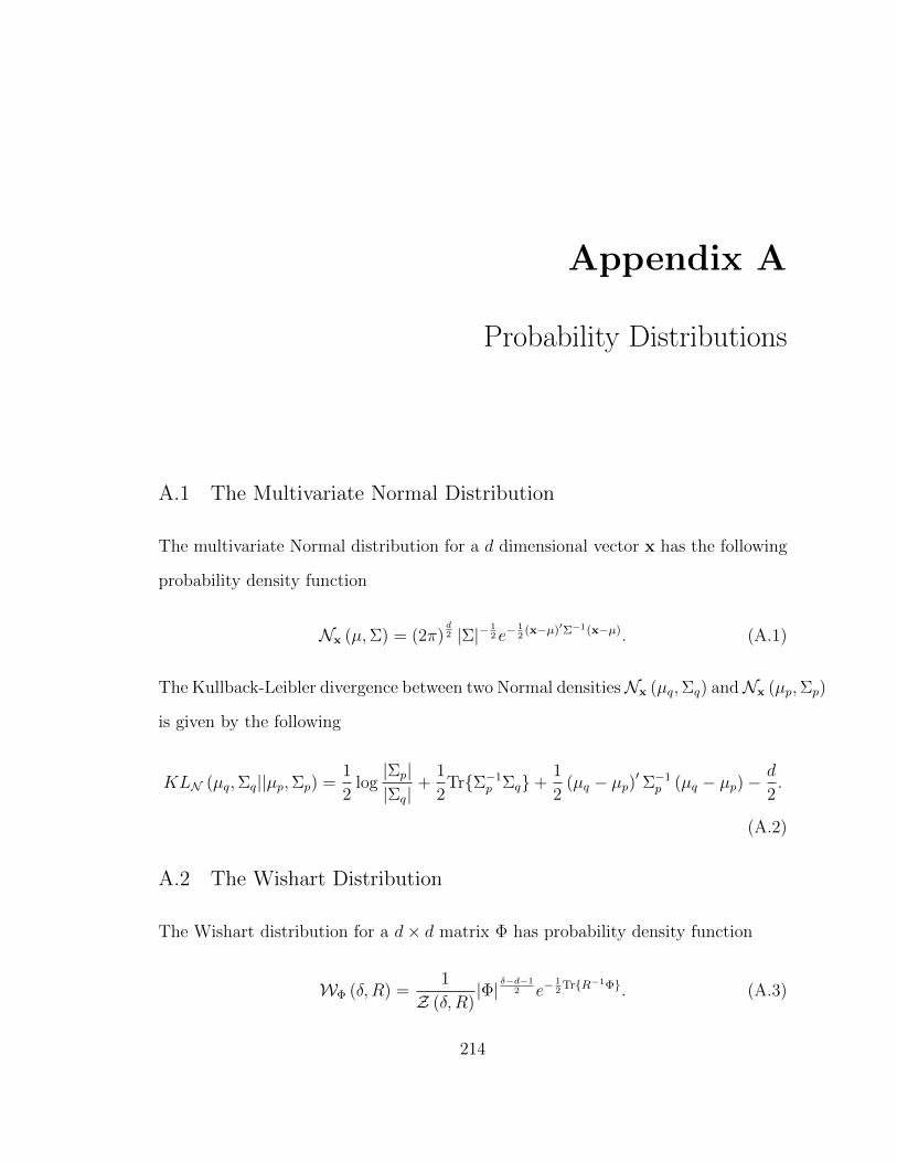
Appendix A

Probability Distributions

A.1 The Multivariate Normal Distribution

The multivariate Normal distribution for a d dimensional vector x has the following

probability density function

Nx (µ,Σ) = (2π)d2 |Σ|−

12 e−

12

(x−µ)′Σ−1(x−µ). (A.1)

The Kullback-Leibler divergence between two Normal densitiesNx (µq,Σq) andNx (µp,Σp)

is given by the following

KLN (µq,Σq||µp,Σp) =1

2log|Σp||Σq|

+1

2TrΣ−1

p Σq+1

2(µq − µp)′Σ−1

p (µq − µp)−d

2.

(A.2)

A.2 The Wishart Distribution

The Wishart distribution for a d× d matrix Φ has probability density function

WΦ (δ, R) =1

Z (δ, R)|Φ|

δ−d−12 e−

12

TrR−1Φ. (A.3)

214

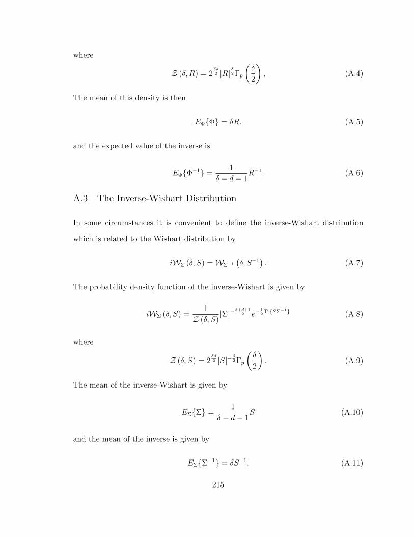
where

Z (δ, R) = 2δd2 |R|

δ2 Γp

(δ

2

), (A.4)

The mean of this density is then

EΦΦ = δR. (A.5)

and the expected value of the inverse is

EΦΦ−1 =1

δ − d− 1R−1. (A.6)

A.3 The Inverse-Wishart Distribution

In some circumstances it is convenient to define the inverse-Wishart distribution

which is related to the Wishart distribution by

iWΣ (δ, S) =WΣ−1

(δ, S−1

). (A.7)

The probability density function of the inverse-Wishart is given by

iWΣ (δ, S) =1

Z (δ, S)|Σ|−

δ+d+12 e−

12

TrSΣ−1 (A.8)

where

Z (δ, S) = 2δd2 |S|−

δ2 Γp

(δ

2

). (A.9)

The mean of the inverse-Wishart is given by

EΣΣ =1

δ − d− 1S (A.10)

and the mean of the inverse is given by

EΣΣ−1 = δS−1. (A.11)

215

Another useful moment of the inverse-Wishart density is the log of the determinant

of the matrix.

EΣlog|Σ| = −d log 2−d∑i=1

Ψ

(δ − i+ 1

2

)+ log|S| (A.12)

The Kullback-Leibler divergence between two inverse-Wishart densities iWΦ (q,Q)

and iWΦ (p, P ) is given by the following

KLiW (q,Q||p, P ) =d∑i=1

(log Γ

(p+ 1− i

2

)− log Γ

(q + 1− i

2

))

+(q

2− p

2

) d∑i=1

Ψ

(q + 1− i

2

)+q

2log|P | − q

2log|Q|

+q

2

(Tr(P−1Q

)− d).

(A.13)

A.4 The Normal-Inverse-Wishart Distribution

If a set of random variables a ∈ R1×m and r ∈ R are distributed Normal-inverse-

Wishart with parameters V and ν their joint probability density is

N iWa,r (V, ν) =r−

ν2

Z (V, ν)e−

12r

[−1,a]V[−1,a]′ . (A.14)

The m+ 1×m+ 1 matrix V can be partitioned into sub-matrices to ease notation,

V =

[V11 V′a1

Va1 Vaa

](A.15)

where the sub-matrices have the following dimensions.

V11 ∈ R

Va1 ∈ Rm×1

Vaa ∈ Rm×m

(A.16)

216

The normalizing constant can then be expressed as

Z (V, ν) = Γ

(−1

2(ν −m− 1)

)λ−

12

(ν−m−1)|Vaa|−12 2

12

(ν−2)πm2 (A.17)

where

λ = V11 −V′a1V−1aa Va1. (A.18)

From these definitions the conditional and marginal distributions can be easily de-

fined.

f (a|r,V, ν) = Na

(V−1aa Va1, rV

−1aa

)(A.19)

f (r|V, ν) = iWr (ν −m− 2, λ) (A.20)

The VB method may required several moments of the Normal-inverse-Wishart.∫log rf (r|V, ν) dr = ψΓ

(ν −m− 2

2

)+ log λ− log 2 (A.21)

∫1

rf (r|V, ν) dr = (ν −m− 2)λ−1 (A.22)

∫af (a|r,V, ν) da = a = V−1

aa Vad (A.23)

∫aa′f (a|r,V, ν) da = rV−1

aa + aa′ (A.24)

217

The Kullback-Leibler divergence between two Normal-inverse-Wishart densitiesN iWar (Q, q)

and N iWar (P, p) is derived as follows.

KLN iW (Q, q||P, p) =

∫∫N iWa,r (Q, q) log

N iWa,r (Q, q)

logN iWa,r (P, p)drda

=

∫∫Na|r (aq, rRq) iWr (ηq, λq) log

Na|r (aq, rRq)

Na|r (ap, rRp)drda

+

∫∫Na|r (aq, rRq) iWr (ηq, λq) log

iWr (ηq, λq)

iWr (ηp, λp)drda

=1

2(aq − ap)

′R−1p (aq − ap)

∫1

riWr (ηq, λq) dr − m

2

+1

2log|Rp||Rq|

+1

2TrR−1

p Rq+KLiWr (ηq, λq||ηp, λp) (A.25)

In these equations the following definitions are used for brevity.

Rp = P−1aa , (A.26)

Rq = Q−1aa , (A.27)

ηp = p−m− 2, (A.28)

ηq = q −m− 2. (A.29)

Using Equation (A.22) we arrive at the final definition of the Kullback-Leibler diver-

gence between two Normal-inverse-Wishart densities.

KLN iW (Q, q||P, p) =ηq

2λq(aq − ap)

′R−1p (aq − ap)−

m

2

+1

2log|Rp||Rq|

+1

2TrR−1

p Rq+KLiWr (ηq, λq||ηp, λp) (A.30)

218

A.5 The Dirichlet Distribution

The probability density function for a random variable α ∈ R1×c, which is distributed

Dirichlet, is given by

f (α|λ) = Dα (λ) =

1

ζ(λ)

c∏i=1

αλi−1i for

c∑i=1

αi = 1

0 otherwise

(A.31)

where

ζ (λ) =

∏ci=1 Γ (λi)

Γ (∑c

i=1 λi). (A.32)

The mean of this density is given by

Ef(α|λ)αi =λi∑cj=1 λj

. (A.33)

The VB method may require the expected value of the log of one of the dimensions

of α. This is given by

Ef(α|λ)logαi = Ψ (λi)−Ψ

(c∑j=1

λj

). (A.34)

The Kullback-Leilber divergence between two Dirichlet densities Dq (λq) and Dp (λp)

is given by the following

KLD (λq||λp) = logΓ(∑c

j=1 λqj

)Γ(∑c

j=1 λpj

) +c∑j=1

logΓ(λpj)

Γ(λqj)

+c∑j=1

((λqj − λ

pj

)(Ψ(λqj)−Ψ

(c∑

k=1

λqk

))).

(A.35)

A.6 The Beta Distribution

The beta distribution is a special case of the Dirichlet distribution with c = 2.

Therefore, the beta distribution is used to model the probability of the occurance of

219

an event, or a value between 0 and 1. The probability density function for a random

variable p ∈ [0, 1] that is distributed Beta is

f (p|a, b) = βp (a, b) =

1

ζ(a,b)p(a−1) (1− p)(b−1) for 0 ≤ p ≤ 1

0 otherwise(A.36)

where

ζ (a, b) =Γ (a) Γ (b)

Γ (a+ b). (A.37)

From the definitions for the Dirichlet density above, the expected value of p is

Ef(p|a,b)p =a

a+ b(A.38)

and the expected value of the log of p is

Ef(p|a,b)log p = Ψ (a)−Ψ (a+ b) . (A.39)

Similarly, the expected value of the log of 1− p is

Ef(p|a,b)log (1− p) = Ψ (b)−Ψ (a+ b) . (A.40)

A.7 Student’s T Distribution

A random variable x ∈ R1×p is said to follow a Student’s T distribution defined by

mean µ, covariance matrix Σ and degrees of freedom n if it has probability density

function as follows.

f (x|µ,Σ, n) =Γ [(n+ p)/2]

Γ(n/2)np/2πp/2 |Σ|1/2[1 + 1

n(x− µ)TΣ−1(x− µ)

](n+p)/2(A.41)

220

Appendix B

Other Required Mathemetical Definitions

B.1 Entropy

The entropy of a probability density function f (θ) is defined as

H (f (θ)) = −∫f (θ) log f (θ) dθ. (B.1)

B.2 The Gamma Function

The Gamma function arises as a generalization of the factorial function and is often

found in probability density functions. It can be expressed as

Γ (x) =

∫ ∞0

tx−1e−tdt. (B.2)

B.3 The Generalized Gamma Function

The generalized Gamma function arises from the a multivariate interpretation of the

Gamma function. Consider t in (B.2) to be a d dimensional positive definite matrix

T . The generalized Gamma function is then

Γ (x) =

∫|T |>0

|T |x−(d−1)/2e−TrTdT (B.3)

221

where the integral is over all possible positive definite matrices. The generalize

Gamma function can be expressed in terms of the Gamma function as

Γd (x) = πd(d−1)

4

d∏j=1

Γ

(x+

1− j2

)(B.4)

B.4 The Digamma Function

The digamma function arises as the derivative of the log of the Gamma function.

It is used, most notably, to calculate the log of the expected value of an element of

a probability vector that is distrubted Dirichlet or a probability that is distributed

Beta. The value of Ψ (x) can be approximated as

Ψ (xλ) =d

dxlog Γ (x) (B.5)

≈ log(x)− 1

2x− 1

12x2+

1

120x4− 1

252x6(B.6)

although better approximations are available in most standard mathematical com-

puting tools.

222

Bibliography

[1] A. Hyvrinen, J. Karhunen, and E. Oja, Independent Component Analysis,1st ed. Wiley-Interscience, May 2001.

[2] Y. Huang, J. Benesty, and J. Chen, Acoustic MIMO Signal Processing.Springer, 2006.

[3] R. Molina, J. Mateos, and A. K. Katsaggelos, “Blind deconvolution using avariational approach to parameter, image, and blur estimation,” Image Pro-cessing, IEEE Transactions on, vol. 15, pp. 3715–3727, 2006.

[4] J. Thomas, Y. Deville, and S. Hosseini, “Time-domain fast fixed-point algo-rithms for convolutive ICA,” IEEE Signal Processing Letters, vol. 13, no. 4, p.228231, 2006.

[5] A. Donzier and J. Millet, “Gunshot acoustic signature specific features andfalse alarms reduction,” in Proceedings of SPIE Vol. 5778, E. M. Carapezza,Ed., vol. 5778, no. 1. SPIE, 2005, pp. 254–263.

[6] G. Lewis, S. Shaw, M. Crowe, C. Cranford, K. Torvik, P. Scharf, andB. Stellingworth, “Urban gunshot and sniper location: technologies anddemonstration results,” E. M. Carapezza, Ed., vol. 4708, no. 1. SPIE, 2002,pp. 315–323.

[7] ShotSpotter Inc., “Shotspotter GLS,” World Wide Web. [Online]. Available:http://www.shotspotter.com/

[8] Saftey Dymanics, “SENTRI (sensor enabled neural threat recognitionand identification),” Wolrd Wide Web. [Online]. Available: http://www.safetydynamics.net/products.html

[9] BBN Technologies, “Boomerang,” World Wide Web. [Online]. Available:http://www.bbn.com/products and services/boomerang/

223

[10] Canberra, “PILAR sniper countermeasures system,” World Wide Web.[Online]. Available: http://www.canberra.com/products/438138.asp

[11] R. C. Maher, “Modeling and signal processing of acoustic gunshot recordings,”Digital Signal Processing Workshop, 12th-Signal Processing Education Work-shop, 4th, pp. 257–261, 2006.

[12] A. Dufaux, L. Besacier, M. Ansortge, and F. Pellandini, “Automatic sounddetection and recognition for noisy environment,” in Proc. of the X EuropeanSignal Processsing Conference, 2000.

[13] D. Hoiem, K. Yan, and R. Sukthankar, “Solar: sound object localization andretrieval in complex audio environments,” in Acoustics, Speech, and SignalProcessing, 2005. Proceedings. (ICASSP ’05). IEEE International Conferenceon, vol. 5, 2005, pp. v/429–v/432 Vol. 5.

[14] G. Guo and S. Z. Li, “Content-based audio classification and retrieval by sup-port vector machines,” Neural Networks, IEEE Transactions on, vol. 14, pp.209–215, 2003.

[15] S. Z. Li, “Content-based classification and retrieval of audio using the nearestfeature line method,” IEEE Transactions on Speech and Audio Processing,vol. 8, pp. 619–625, 2000.

[16] C. Clavel, T. Ehrette, and G. Richard, “Events detection for an audio-basedsurveillance system,” Multimedia and Expo, 2005. ICME 2005. IEEE Interna-tional Conference on, pp. 1306–1309, 2005.

[17] G. Valenzise, G. Valenzise, L. Gerosa, L. Gerosa, M. Tagliasacchi, F. An-tonacci, and A. Sarti, “Scream and gunshot detection and localization foraudio-surveillance systems,” in Advanced Video and Signal Based Surveillance,2007. AVSS 2007. IEEE Conference on, 2007, pp. 21–26.

[18] E. T. Jaynes, Probability Theory: The Logic of Science. Cambridge UniversityPress, Jun. 2003.

[19] T. S. Ferguson, “A Bayesian analysis of some nonparametric problems,” TheAnnals of Statistics, vol. 1, pp. 209–230, Mar. 1973.

[20] J. W. Lau and M. K. P. So, “Bayesian mixture of autoregressive models,”Comput. Stat. Data Anal., vol. 53, no. 1, pp. 38–60, 2008.

224

[21] S. Sampietro, “Bayesian analysis of mixture of autoregressive components withan application to financial market volatility,” Appl. Stoch. Model. Bus. Ind.,vol. 22, no. 3, pp. 225–242, 2006.

[22] J. Sethuraman, “A constructive definition of Dirichlet priors,” Statistica Sinica,vol. 4, pp. 639–650, 1994.

[23] J. Paisley and L. Carin, “Dirichlet process mixture models with multiple modal-ities,” in Proceedings of the 2009 IEEE International Conference on Acoustics,Speech and Signal Processing-Volume 00, 2009, p. 16131616.

[24] Y. W. Teh, M. I. Jordan, M. J. Beal, and D. M. Blei, “Hierarchical Dirichletprocesses,” Journal of the American Statistical Association, vol. 101, no. 476,p. 15661581, 2006.

[25] E. B. Fox, E. B. Sudderth, M. I. Jordan, and A. S. Willsky, “An HDP-HMMfor systems with state persistence,” in Proceedings of the 25th internationalconference on Machine learning. ACM New York, NY, USA, 2008, pp. 312–319.

[26] ——, “Nonparametric Bayesian identification of jump systems with sparse de-pendencies,” in Proc. 15th IFAC Symposium on System Identification, July2009.

[27] Y. Qi, J. W. Paisley, and L. Carin, “Music analysis using hidden Markovmixture models,” Signal Processing, IEEE transactions on, vol. 55, no. 11, p.5209, 2007.

[28] K. Ni, L. Carin, and D. Dunson, “Multi-task learning for sequential data viaiHMMs and the nested Dirichlet process,” in Proceedings of the 24th interna-tional conference on Machine learning, 2007, p. 696.

[29] K. Ni, J. Paisley, L. Carin, and D. Dunson, “Multi-task learning for analyz-ing and sorting large databases of sequential data,” Signal Processing, IEEETransactions on, vol. 56, no. 8, pp. 3918–3931, Aug. 2008.

[30] V. Smıdl and A. Quinn, The Variational Bayes Method in Signal Process-ing (Signals and Communication Technology). Secaucus, NJ, USA: Springer-Verlag New York, Inc., 2005.

[31] C. M. Bishop, Pattern Recognition and Machine Learning, 1st ed. Springer,Oct. 2007.

225

[32] D. J. C. MacKay, Information Theory, Inference, and Learning Algorithms.Cambridge UniversityPress, 2003.

[33] R. E. Kass and A. E. Raftery, “Bayes factors,” Technical Report 254, Depart-ment of Statistics, University of Washington, 1995.

[34] H. Raiffa and R. Schlaifer, Applied Statistical Decision Theory, 1st ed. Wiley-Interscience, May 2000.

[35] D. R. Clark and C. A. Thayer, “A primer on the exponential family of dis-tributions,” Casualty Actuarial Society Discussion Paper Program CasualtyActuarial Society, pp. 117–148, 2004.

[36] A. Dempster, N. Laird, and D. Rubin, “Maximum likelihood from incompletedata via the em algorithm,” Journal of the Royal Statistical Society, vol. 39,pp. 1–38, 1977.

[37] R. P. Feynman, Statistical Mechanics: A Set of Lectures, ser. Advanced bookclassics. Reading, Mass: Addison-Wesley, 1998.

[38] T. S. Jaakkola, Advanced mean field methods: theory and practice. MIT Press,2000, ch. Tutorial on Variational Approximation Methods.

[39] T. S. Jaakkola and M. I. Jordan, “Bayesian parameter estimation throughvariational methods,” Statistics and Computing, vol. 10, pp. 25–37, 1998.

[40] G. E. Hinton and D. van Camp, Neural Information Processing Systems Sys-tems 8. Santa Cruz, California, United States: MIT Press, 1993, ch. Keepingthe neural networks simple by minimizing the description length of the weights,pp. 5–13.

[41] D. MacKay, “Ensemble learning and evidence maximization,” in NIPS, 1995.

[42] S. Waterhouse, D. MacKay, M. Rd, C. B. Cambridge, and T. Robinson,“Bayesian methods for mixtures of experts,” Advances in neural informationprocessing systems, 1996.

[43] J. Winn and C. M. Bishop, “Variational message passing,” The Journal ofMachine Learning Research, vol. 6, pp. 661–694, 2005.

[44] M. aki Sato, “Online model selection based on the variational bayes,” NeuralComp., vol. 13, pp. 1649–1681, Jul. 2001.

226

[45] R. A. Choudrey, “Variational methods for bayesian independent componentanalysis,” Ph.D. dissertation, University of Oxford, 2002.

[46] M. J. Beal, “Variational algorithms for approximate bayesian inference,” Ph.D.dissertation, Gatsby Computational Neuroscience Unit, University CollegeLondon, 2003.

[47] N. D. Le, L. Sun, and J. V. Zidek, “Bayesian spatial interpolation andbackcasting using gaussian-generalized inverted wishart model,” Univ. BritishColumbia, Vancouver, BC, Canada, Tech. Rep, 1999.

[48] M. S. Arulampalam, S. Maskell, N. Gordon, and T. Clapp, “A tutorial on par-ticle filters for online nonlinear/non-gaussian bayesian tracking,” IEEE Trans-actions on Signal Processing, vol. 50, pp. 174–188, 2002.

[49] R. Kulhavy and M. B. Zarrop, “On a general concept of forgetting,” Interna-tional Journal of Control, vol. 58, pp. 905–924, 1993.

[50] A. Honkela and H. Valpola, “On-line variational bayesian learning,” Proceed-ings of the 4th International Symposium on Independent Component Analysisand Blind Signal Separation (ICA2003), pp. 803–808, 2003.

[51] R. Kulhavy, “Restricted exponential forgetting in real-time identification,” Au-tomatica, vol. 23, pp. 589–600, Sep. 1987.

[52] V. Smıdl and A. Quinn, “Bayesian estimation of non-stationary ar model pa-rameters via an unknown forgetting factor,” Digital Signal Processing Work-shop, 2004 and the 3rd IEEE Signal Processing Education Workshop. 2004IEEE 11th, pp. 221–225, 2004.

[53] S. Haykin, Adaptive Filter Theory, 4th ed. Prentice Hall, Sep. 2001.

[54] W. D. Penny and S. J. Roberts, “Bayesian methods for autoregressive models,”Neural Networks for Signal Processing X, 2000. Proceedings of the 2000 IEEESignal Processing Society Workshop, vol. 1, 2000.

[55] V. Smıdl and A. Quinn, “The variational EM algorithm for on-line identifica-tion of extended AR models,” Acoustics, Speech, and Signal Processing, 2005.Proceedings.(ICASSP’05). IEEE International Conference on, vol. 4, 2005.

[56] ——, “Mixture-based extension of the AR model and its recursive Bayesianidentification,” Signal Processing, IEEE Transactions on, vol. 53, pp. 3530–3542, 2005.

227

[57] V. Smıdl, A. Quinn, M. Karny, and T. V. Guy, “Robust estimation of au-toregressive processes using a mixture-based filter-bank,” Systems & ControlLetters, vol. 54, pp. 315–323, 2005.

[58] A. Gelman, Bayesian Data Analysis. CRC Press, 2004.

[59] H. Akaike, “Fitting autoregressive models for prediction,” Annals of the Insti-tute of Statistical Mathematics, vol. 21, pp. 243–247, 1969.

[60] G. Schwarz, “Estimating the dimension of a model,” Annals of Statistics, vol. 6,pp. 461–464, 1978.

[61] C. M. Bishop and M. E. Tipping, “Variational relevance vector machines,” inProceedings of the 16th Conference on Uncertainty in Artificial Intelligence.San Francisco: Morgan Kaufmann Publishers, 2000, p. 4653.

[62] C. S. Wong and W. K. Li, “On a mixture autoregressive model,” Journal of theRoyal Statistical Society. Series B, Statistical Methodology, pp. 95–115, 2000.

[63] ——, “On a mixture autoregressive conditional heteroscedastic model,” Jour-nal of the American Statistical Association, vol. 96, no. 455, pp. 982–995, 2001.

[64] ——, “On a logistic mixture autoregressive model,” Biometrika, vol. 88, no. 3,pp. 833–846, 2001.

[65] P. W. Fong, W. K. Li, C. W. Yau, and C. S. Wong, “On a mixture vector au-toregressive model,” The Canadian Journal of Statistics/La revue canadiennede statistique, vol. 35, no. 1, pp. 135–150, 2007.

[66] Y. Xiong and D. Y. Yeung, “Mixtures of ARMA models for model-based timeseries clustering,” in Proceedings of the IEEE International Conference on DataMining. ICDM, 2002, pp. 717–720.

[67] S. Roberts and W. Penny, “Variational Bayes for generalized autoregressivemodels,” Signal Processing, IEEE Transactions on, vol. 50, pp. 2245–2257,2002.

[68] C. E. Antoniak, “Mixtures of Dirichlet processes with applications to Bayesiannonparametric problems,” Annals of Statistics, vol. 2, pp. 1152–1174, 1974.

[69] E. B. Fox, E. B. Sudderth, M. I. Jordan, and A. S. Willsky, “NonparametricBayesian learning of switching linear dynamical systems,” in Advances in Neu-ral Information Processing Systems (NIPS), D. S. D. Koller, Y. Bengio andL. Bottou, Eds., vol. 21, 2008.

228

[70] E. Punskaya, C. Andrieu, A. Doucet, and W. J. Fitzgerald, “Bayesian curvefitting using MCMC with applications to signal segmentation,” IEEE Trans-actions on Signal Processing, vol. 50, no. 3, p. 747758, 2002.

[71] M. E. Tipping, “Sparse Bayesian learning and the relevance vector machine,”Journal of Machine Learning Research, vol. 1, pp. 211–244, 2001.

[72] D. J. C. MacKay and R. M. Neal, “Automatic relevance determination forneural networks.” Technical Report In preparation, Cambridge University,1994.

[73] C. M. Hurvich and C. Tsai, “Regression and time series model selection insmall samples,” Biometrika, vol. 76, no. 2, pp. 297–307, Jun. 1989. [Online].Available: http://biomet.oxfordjournals.org/cgi/content/abstract/76/2/297

[74] Y. Qi and T. S. Jaakkola, “Parameter expanded variational Bayesian methods,”Advances in Neural Information Processing Systems, vol. 19, p. 1097, 2007.

[75] S. N. MacEachern, Computational methods for mixture of Dirichlet processmodels. Springer, 1998, ch. 2, pp. 23–43.

[76] R. M. Neal, “Markov chain sampling methods for Dirichlet process mixturemodels,” Journal of Computational and Graphical Statistics, vol. 9, pp. 249–265, 2000.

[77] D. M. Blei and M. I. Jordan, “Variational methods for the Dirichlet process,” inProceedings of the 21st International Conference on Machine Learning. Banff,Alberta, Canada: ACM, 2004, p. 12.

[78] ——, “Variational inference for Dirichlet process mixtures,” Bayesian Analysis,vol. 1, pp. 121–144, 2006.

[79] K. Kurihara, M. Welling, and Y. W. Teh, “Collapsed variational Dirichlet pro-cess mixture models,” International Joint Conference on Artificial Intelligence,2007.

[80] K. Kurihara, M. Welling, and N. Vlassis, “Accelerated variational Dirichletprocess mixtures,” Advances in Neural Information Processing Systems, vol. 19,p. 761768, 2007.

[81] D. Blackwell and J. B. MacQueen, “Ferguson distributions via Polya urnschemes,” Ann. Statist, vol. 1, pp. 353–355, 1973.

229

[82] H. Ishwaran and L. F. James, “Gibbs sampling methods for Stick-Breakingpriors.” Journal of the American Statistical Association, vol. 96, no. 453, 2001.

[83] R. O. Duda, P. E. Hart, and D. G. Stork, Pattern Classification, 2nd ed.Wiley-Interscience, Oct. 2000.

[84] L. R. Rabiner, “A tutorial on hidden Markov models and selected applicationsin speech recognition,” Proceedings of the IEEE, vol. 77, pp. 257–286, 1989.

[85] Y. Qi, J. Paisley, and L. Carin, “Dirichlet process HMM mixture models withapplication to music analysis,” in Acoustics, Speech and Signal Processing,2007. ICASSP 2007. IEEE International Conference on, vol. 2, 2007, pp. II–465–II–468.

[86] M. J. Beal, Z. Ghahramani, and C. E. Rasmussen, “The infinite hidden markovmodel,” Advances in Neural Information Processing Systems, vol. 14, pp. 577–584, 2002.

[87] J. J. R. Deller, J. G. Proakis, and J. H. L. Hansen, Discrete-Time Processingof Speech Signals. New York: Maxmillan Publishing Company, 1993.

[88] R. Lyon, “Computational models of neural auditory processing,” in IEEE In-ternational Conference on Acoustics, Speech, and Signal Processing, vol. 9,1984, pp. 41–44.

[89] S. Seneff, “A joint synchrony/mean-rate model of auditory speech processing,”Readings in Speech Recognition, pp. 101–111, 1988.

[90] P. Torrione and L. Collins, “Texture features for antitank landmine detectionusing ground penetrating radar,” IEEE Transactions on Geoscience and Re-mote Sensing, vol. 45, pp. 2374–2382, 2007.

[91] H. Frigui and P. Gader, “Detection and discrimination of land mines in ground-penetrating radar based on edge histogram descriptors and a possibilistic k-nearest neighbor classifier,” Fuzzy Systems, IEEE Transactions on, vol. 17,no. 1, pp. 185–199, Feb. 2009.

[92] P. Torrione and L. Collins, “Application of markov random fields to landminedetection in ground penetrating radar data,” in Proceedings of the SPIE, De-tection and Sensing of Mines, Explosive Objects, and Obscured Targets XIII.,R. S. Harmon, J. Holloway, John H., and J. T. Broach, Eds., vol. 6953, 2008,pp. 69 531B–69 531B–12.

230

[93] F. Roth, P. van Genderen, M. Verhaegen, S. R. Center, and F. Clamart, “Con-volutional models for buried target characterization with ground penetratingradar,” IEEE Transactions on Antennas and Propagation, vol. 53, no. 11, p.37993810, 2005.

[94] K. Ho, L. Carin, P. Gader, and J. Wilson, “An investigation of using the spec-tral characteristics from ground penetrating radar for landmine/clutter dis-crimination,” Geoscience and Remote Sensing, IEEE Transactions on, vol. 46,no. 4, pp. 1177–1191, April 2008.

[95] K. J. Hintz, N. Peixoto, and D. Hwang, “Syntactic landmine detectionand classification,” in Proceedings of SPIE, Orlando, FL, USA, 2009,pp. 730 322–730 322–9. [Online]. Available: http://link.aip.org/link/PSISDG/v7303/i1/p730322/s1&Agg=doi

[96] Y. Xiong and D. Yeung, “Time series clustering with ARMA mixtures,”Pattern Recognition, vol. 37, no. 8, pp. 1675–1689, Aug. 2004. [Online]. Avail-able: http://www.sciencedirect.com/science/article/B6V14-4C5HPCX-2/2/7ae274523d5059d498734f0967dbb482

[97] D. Garcia-Garcia, E. P. Hernandez, and F. D. de Maria, “A new distancemeasure for Model-Based sequence clustering,” Pattern Analysis and MachineIntelligence, IEEE Transactions on, vol. 31, no. 7, pp. 1325–1331, 2009.[Online]. Available: http://portal.acm.org/citation.cfm?id=1550662

[98] M. I. Jordan, Frontiers of Statistical Decision Making and Bayesian Analysis—In Honor of James O. Berger. New York: Springer, 2010, ch. Hierarchicalmodels, nested models and completely random measures.

[99] D. M. Blei, T. L. Griffiths, and M. I. Jordan, “The nested chinese restaurantprocess and hierarchical topic models. 2007,” Advances in Neural InformationProcessing Systems, vol. 710, 2004.

[100] A. Rodriguez, D. B. Dunson, and A. E. Gelfand, “The nested dirichlet process,”Journal of the American Statistical Association, vol. 103, no. 483, p. 11311154,2008.

[101] N. X. Vinh, J. Epps, and J. Bailey, “Information theoretic measuresfor clusterings comparison: is a correction for chance necessary?” inProceedings of the 26th Annual International Conference on Machine Learning.Montreal, Quebec, Canada: ACM, 2009, pp. 1073–1080. [Online]. Available:http://portal.acm.org/citation.cfm?id=1553511

231

[102] S. Ntalampiras, I. Potamitis, and N. Fakotakis, “Exploiting temporal featureintegration for generalized sound recognition,” EURASIP Journal on Advancesin Signal Processing, vol. 2009, p. 12, 2009.

[103] B. M. Sadler, T. Pham, and L. C. Sadler, “Optimal and wavelet-based shockwave detection and estimation,” The Journal of the Acoustical Society of Amer-ica, vol. 104, pp. 955–963, 1998.

[104] W. D. Penny and S. J. Roberts, “Bayesian multivariate autoregressive modelswith structured priors,” Vision, Image and Signal Processing, IEE Proceedings-, vol. 149, pp. 33–41, 2002.

[105] L. Harrison, W. D. Penny, and K. Friston, “Multivariate autoregressive mod-eling of fmri time series,” Neuroimage, vol. 19, pp. 1477–1491, 2003.

[106] P. Orbanz and J. M. Buhmann, “Nonparametric bayesian image segmenta-tion,” International Journal of Computer Vision, vol. 77, no. 1, p. 2545, 2008.

[107] L. L. Freeman and A. Torralba, “Nonparametric bayesian texture learning andsynthesis,” Neural Infromation Processing Symposium, vol. 2008, 2008.

[108] E. B. Sudderth and M. I. Jordan, “Shared segmentation of natural scenes usingdependent pitman-yor processes,” in NIPS, 2008, pp. 1585–1592.

[109] L. Ren, L. Du, L. Carin, and D. B. Dunson, “Logistic Stick-Breaking process,”Neural Information Processing Symposium, vol. 2010, 2010.

[110] C. Stauffer and W. E. Grimson, “Adaptive background mixture models forreal-time tracking,” in Proceedings of the IEEE Computer Society Conferenceon Computer Vision and Pattern Recognition, vol. 2, 1999, p. 246252.

[111] Z. Zivkovic, “Improved adaptive gaussian mixture model for background sub-traction,” in Proceedings of the 17th International Conference on PatternRecognition, vol. 2, 2004, p. 2831.

[112] Y. Lin and D. Lee, “Relevant deconvolution for acoustic source estimation,”in Acoustics, Speech, and Signal Processing, 2005. Proceedings. (ICASSP ’05).IEEE International Conference on, vol. 5, 2005, pp. v/529–v/532 Vol. 5.

[113] Q. Huang, J. Yang, and S. Wei, “Temporally correlated source separation usingvariational bayesian learning approach,” Digit. Signal Process., vol. 17, pp.873–890, 2007.

232

Biography

Kenneth D. Morton Jr. was born in York, PA, on October 18, 1982. He received the

B.S. degree in electrical and computer engineering from The University of Pittsburgh,

Pittsburgh, PA, in 2004, and the M.S. and Ph.D. degrees in electrical and computer

engineering from Duke University, Durham, NC, in 2006 and 2010.

He is a devout Bayesian and a practicing engineer as part owner of New Folder

Consulting. He is primarily interested in using modern statistical techniques to solve

problems.

Mr. Morton is a member of Tau Beta Pi and Eta Kappa Nu.

233