Bayesian prediction of the transient behaviour and busy period in short- and long-tailed queueing systems

Bayesian prediction of the transient behaviour and busy period in

short and long-tailed GI/G/1 queueing systems.

M. Concepcion Ausın,∗

Department of Mathematics, Universidade da Coruna,15071 A Coruna, Spain.

Michael P. Wiper, Rosa E. LilloDepartment of Statistics, Universidad Carlos III de Madrid,

28903 Getafe, Madrid, Spain.

Abstract

Bayesian inference for the transient behavior and duration of a busy period in a single server queueingsystem with general, unknown distributions for the interarrival and service times is investigated. Boththe interarrival and service time distributions are approximated using the dense family of Coxian dis-tributions. A suitable reparameterization allows the definition of a non-informative prior and Bayesianinference is then undertaken using reversible jump Markov chain Monte Carlo methods. An advantage ofthe proposed procedure is that heavy tailed interarrival and service time distributions such as the Paretocan be well approximated. The proposed procedure for estimating the system measures is based onrecent theoretical results for the Coxian/Coxian/1 system. A numerical technique is developed for everyMCMC iteration so that the transient queue length and waiting time distributions and the duration ofa busy period can be estimated. The approach is illustrated with both simulated and real data.

Keywords: Bayesian inference, Coxian distribution, heavy tails, queueing systems, semiparametricmodelling, transient analysis, reversible jump.

1Corresponding author. M. C. Ausın, Departamento of Matematicas, Facultad de Informatica, Campus de Elvina, Uni-versidade da Coruna, 15071 A Coruna, Spain. Tel.: +34 981 167 000 (ext. 1301); fax: + 34 981 167 160. E-mail address:[email protected]

1

1 Introduction

Bayesian estimation of stationary distributions in queueing systems is a well developed research area. Someuseful references are Armero and Bayarri (1994, 1997), Rios et al. (1998), Wiper (1998), Armero and Conesa(2000) and Ausın et al. (2003, 2004). However, less progress has been made on the estimation of the transientbehaviour although in many practical situations, the analysis of a queueing system in the transient states isof great interest, for example, when the system is regularly stopped and started again, or when convergenceto steady-state is very slow. Furthermore, the estimation of the duration of a busy period has also beenneglected in the Bayesian literature on queues although the study of the busy period distribution is veryimportant in optimal control problems. Exceptions are Armero and Bayarri (1994, 1997) who consider thebusy period for the M/M/1 system and the transient distribution for the M/M/∞ system, respectively, andAusın et al. (2004) who consider the busy period of the M/G/1 system. Although exact results for thetransient behaviour and busy period of Markovian systems are known, see e.g. Gross and Harris (1985), suchsystems are rarely found in practice. One of the contributions of this article is the estimation of the transientbehaviour and busy period distribution of a much more general queueing system.

It is well known that many measures in communication systems such as packet interarrival times, filelengths or intervals between connection requests in Internet traffic, have long-tailed distributions, see e.g.Paxson and Floyd (1995) and Crovella et al. (1997). These measures are usually described with distributionssuch as the Pareto or Weibull. Unfortunately, queueing systems with long-tailed interarrival or service timedistributions are very difficult to analyze due to the non-existence of their moments or the lack of Laplacetransforms with explicit expressions, see e.g. Abate et al. (1994). As an alternative, Feldmann and Whitt(1998) and Riska et al. (2004) propose approximating long-tailed distributions using hyperexponential den-sities and mixtures of Erlang distributions, respectively, and apply these approximations to the analysis ofqueueing systems using classical statistical methodology. Bayesian inference for hyperexponential distribu-tions and mixtures of Erlang distributions has been considered in Rios et al. (1998) and Ausın et al. (2004),respectively. However, due to the influence of the proper prior distributions, these approaches cannot prop-erly approximate long-tailed interarrival or service time distributions. In contrast, in this article, the modeland prior formulation used permits us to well approximate long-tailed distributions.

Throughout, we shall use the Coxian family of distributions as a semiparametric approximation to theinterarrival and service time distributions. This family includes the standard distributions usually studiedin queueing theory, such as the exponential, Erlang and hyperexponential distribution, as special cases. TheCoxian family is dense over the set of distributions on the positive reals, see e.g. Bertsimas (1990), and thus,any continuous and positive distribution can be approximated arbitrarily closely. Furthermore, based onthe Cox’s method of stages, see Cox (1955), many results for systems with Coxian distributions have beenobtained in the queueing literature. In particular, in this paper we will consider results derived by Bertsimasand Nakazato (1992) for the transient behaviour and busy period.

Bayesian inference for the Coxian distribution was considered in Ausın et al. (2003), in the context ofa hospital resource allocation problem equivalent to a M/G/c/K, finite capacity, Poisson arrivals, queueingsystem. In that article, a different parameterization and approach to that used here was applied. There, aproper prior was assumed and semi-conjugate inference was developed using latent variables. Unfortunately,this setup leads to poor approximations of long-tailed distributions. Furthermore, the Coxian model consid-ered in Ausın et al. (2003) is not identifiable which often affects the convergence of the MCMC algorithmand the interpretation of the estimated parameters. Finally, transient and busy period problems were notanalyzed. Here, we propose a new parameterization which provides an identifiable Coxian model where animproper prior distribution can be applied which leads to good performance of the MCMC algorithm andwhich allows us to well approximate both short and long-tailed distributions.

The rest of this paper is organized as follows. In Section 2, we introduce the Coxian distribution modeland then describe how to carry out Bayesian inference for this model given an improper prior and using areversible jump MCMC algorithm, see Green (1995) and Richardson and Green (1997). In Section 3, wedescribe some results derived by Bertsimas and Nakazato (1992) which allow us to estimate the transientand busy period distributions of the Coxian/Coxian/1 system conditional on the system parameters. Then,

2

-

&%

'$

λ1

?

-

P1

&%

'$

λ2

?P2

- · · · -

&%

'$

λL−1

?PL−1

-

&%

'$

?

λL

PL

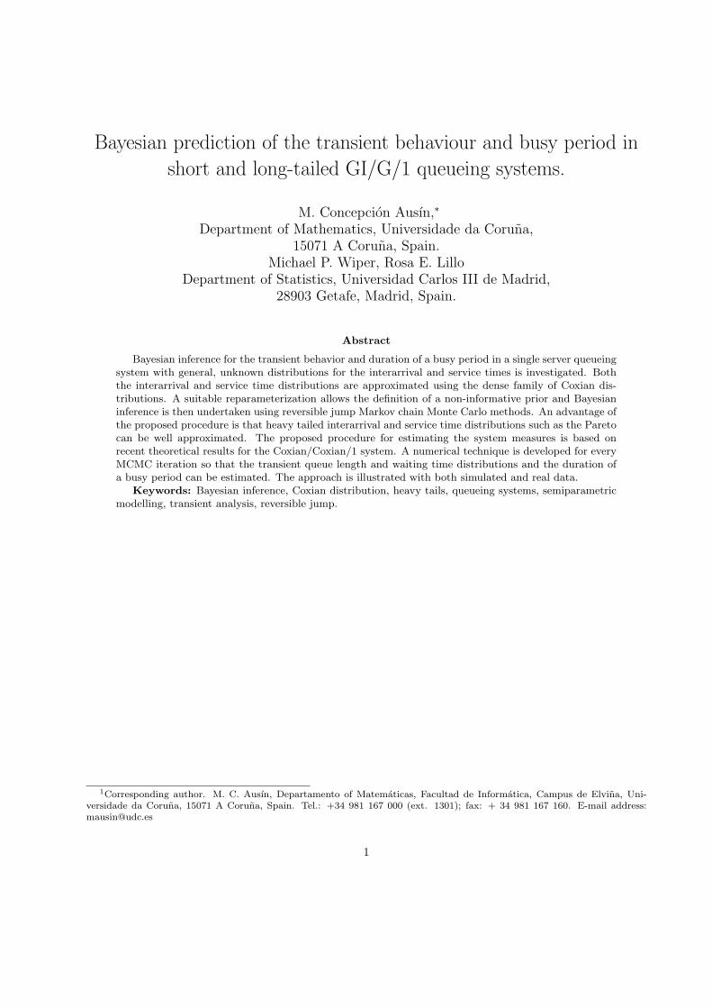
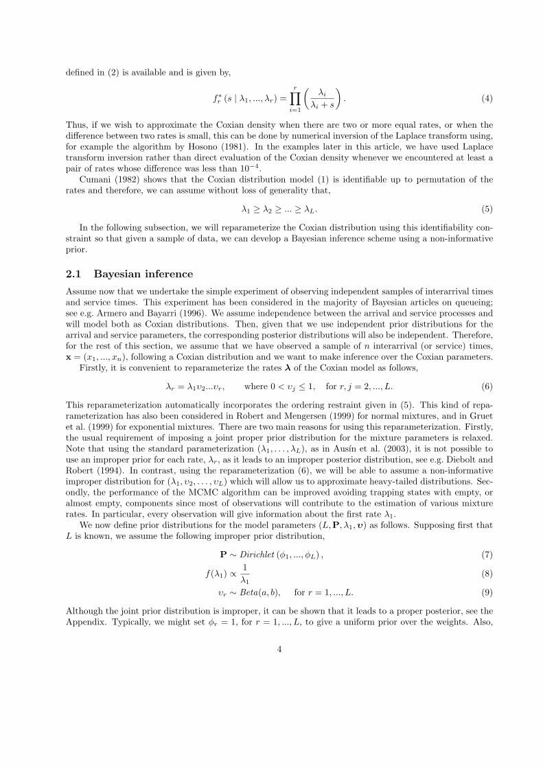
Figure 1: Phase diagram of the Coxian distribution which, with probability Pr, is a sum of r exponentialrandom variables with rates λ1, . . . , λr, for r = 1, . . . , L.

we explain a numerical procedure which allows us to incorporate these results within the reversible jumpalgorithm so that we can estimate the predictive transient and busy period distributions given a sample ofinterarrival and service data. At the end of both Section 2 and Section 3, our approach is illustrated withsimulated and real interarrival and service time data. The paper finishes with some brief conclusions andextensions.

2 Modelling and inference for the interarrival and service times

Firstly we will define the Coxian distribution that we shall use throughout to model the interarrival andservice time data. The Coxian or Mixed Generalized Erlang distribution (MGE), is defined as follows.A positive random variable, X, has a Coxian distribution with parameters L, P = (P1, ..., PL) and λ =(λ1, ..., λL), if,

X =

Y1, with probability = P1,Y1 + Y2, with probability = P2,...

...Y1 + ... + YL, with probability = PL,

(1)

where Yr has an exponential distribution with parameter λr, Pr, λr > 0 and∑L

r=1Pr = 1, see e.g. Bertsimasand Nakazato (1992). This model has a nice visual representation, see Figure 1, where it can be seen thatthe interarrival (or service) time of each customer can be represented by a sequence of a random number ofexponential stages.

The Coxian distribution model (1) can also be expressed in mixture form,

f (x | L,P,λ) =L∑

r=1Prfr (x | λ1, ..., λr) , x ≥ 0, (2)

where fr (x | λ1, ..., λr) is the density of a generalized Erlang distribution, i.e. the density of a sum of rexponential random variables with rates λ1, λ2, ..., λr respectively. If all rates are unequal, this density isgiven by,

fr (x | λ1, ..., λr) =r∑

j=1

r∏

i=1i 6=j

λi

λi − λj

λj exp (−λjx) , x ≥ 0, (3)

see e.g. Johnson and Kotz (1970). In some cases where there are two or more equal rates, alternativeexpressions can be derived, e.g. if all rates are equal, the Coxian density reduces to an Erlang, but a generalformula for all possible cases is not known. However, the Laplace transform of the Coxian distribution

3

defined in (2) is available and is given by,

f∗r (s | λ1, ..., λr) =r∏

i=1

(λi

λi + s

). (4)

Thus, if we wish to approximate the Coxian density when there are two or more equal rates, or when thedifference between two rates is small, this can be done by numerical inversion of the Laplace transform using,for example the algorithm by Hosono (1981). In the examples later in this article, we have used Laplacetransform inversion rather than direct evaluation of the Coxian density whenever we encountered at least apair of rates whose difference was less than 10−4.

Cumani (1982) shows that the Coxian distribution model (1) is identifiable up to permutation of therates and therefore, we can assume without loss of generality that,

λ1 ≥ λ2 ≥ ... ≥ λL. (5)

In the following subsection, we will reparameterize the Coxian distribution using this identifiability con-straint so that given a sample of data, we can develop a Bayesian inference scheme using a non-informativeprior.

2.1 Bayesian inference

Assume now that we undertake the simple experiment of observing independent samples of interarrival timesand service times. This experiment has been considered in the majority of Bayesian articles on queueing;see e.g. Armero and Bayarri (1996). We assume independence between the arrival and service processes andwill model both as Coxian distributions. Then, given that we use independent prior distributions for thearrival and service parameters, the corresponding posterior distributions will also be independent. Therefore,for the rest of this section, we assume that we have observed a sample of n interarrival (or service) times,x = (x1, ..., xn), following a Coxian distribution and we want to make inference over the Coxian parameters.

Firstly, it is convenient to reparameterize the rates λ of the Coxian model as follows,

λr = λ1υ2...υr, where 0 < υj ≤ 1, for r, j = 2, ..., L. (6)

This reparameterization automatically incorporates the ordering restraint given in (5). This kind of repa-rameterization has also been considered in Robert and Mengersen (1999) for normal mixtures, and in Gruetet al. (1999) for exponential mixtures. There are two main reasons for using this reparameterization. Firstly,the usual requirement of imposing a joint proper prior distribution for the mixture parameters is relaxed.Note that using the standard parameterization (λ1, . . . , λL), as in Ausın et al. (2003), it is not possible touse an improper prior for each rate, λr, as it leads to an improper posterior distribution, see e.g. Diebolt andRobert (1994). In contrast, using the reparameterization (6), we will be able to assume a non-informativeimproper distribution for (λ1, υ2, . . . , υL) which will allow us to approximate heavy-tailed distributions. Sec-ondly, the performance of the MCMC algorithm can be improved avoiding trapping states with empty, oralmost empty, components since most of observations will contribute to the estimation of various mixturerates. In particular, every observation will give information about the first rate λ1.

We now define prior distributions for the model parameters (L,P, λ1, υ) as follows. Supposing first thatL is known, we assume the following improper prior distribution,

P ∼ Dirichlet (φ1, ..., φL) , (7)

f(λ1) ∝ 1λ1

(8)

υr ∼ Beta(a, b), for r = 1, ..., L. (9)

Although the joint prior distribution is improper, it can be shown that it leads to a proper posterior, see theAppendix. Typically, we might set φr = 1, for r = 1, ..., L, to give a uniform prior over the weights. Also,

4

we might set a = b = 1 to give a uniform prior over each υr, for r = 1, ..., L. However, it is necessary toset a > 1 in order that the posterior predictive mean of the Coxian variable, X, exists, as is shown in theAppendix. Then, we have set a = 1.1 and b = 1 in the examples.

This type of parameterization and prior choice allows us to approximate long-tailed distributions as willbe shown in the examples. This is because we do not make a strong assumption about the rate of the firstcomponent, λ1, and consequently, the means of the various mixture components can be as small or as largeas required.

Our task is now to construct an MCMC algorithm to sample from the joint posterior distribution whichis obtained from the prior distributions, (7), (8) and (9), and the likelihood function,

l (θ | x) =n∏

i=1

(L∑

r=1

Prfr (xi | λ1, υ2, . . . , υr)

), (10)

where θ = (L,P, λ1, υ) and where from now on we use fr (x | λ1, υ2, ..., υr) to denote the reparameterizedCoxian density fr(x | λ1, λ2, .., λr) given in (2). As is usually done in mixture models, see e.g. Diebolt andRobert (1994), we use a data augmentation algorithm, introducing for each datum, xi, component indicatorvariables, Zi, such that,

P (Zi = r | L,P) = Pr, f (xi | Zi = r) = fr (xi | λ1, υ2, . . . , υr)

for i = 1, ..., n. Then, we obtain that,

P (Zi = r | xi,P, λ1, υ) ∝ Prfr (xi | λ1, υ2, ..., υr) , for r = 1, ..., L, (11)

for i = 1, ..., n, where fr is evaluated by using (3) or inverting (4) as commented above. With this approach,every observed data set, x = {x1, . . . , xn} is associated to a missing data set, z = {z1, . . . , zn}, indicatingthe specific components of the mixture from which the observations are assumed to arise. Given the missingdata, the likelihood (10) is simplified to,

l (θ | x, z) ∝n∏

i=1

Pzifzi (xi | λ1, υ2, . . . , υzi) . (12)

From (7) and (12), the conditional posterior distribution of the weights is given by,

P | x, z ∼ Dirichlet(1 + n1, ..., 1 + nL), (13)

where nr is the number of data assigned to the r’th mixture component for r = 1, ..., L. From (8), (9) and(12), we obtain the conditional posterior distributions of λ1 and υ, which do not have explicit expressionsbut their density functions can be evaluated up to the integration constants as,

f (λ1 | x, z, υ) ∝n∏

i=1

fzi (xi | λ1, υ2, . . . , υzi) f (λ1) , (14)

f (υr | x, z,λ1, υ−r) ∝n∏

i=1zi≥r

fzi (xi | λ1, υ2, . . . , υzi) f (υr) , for r = 2, . . . , L. (15)

Thus, we can now use Gibbs sampling scheme to generate a sample from the posterior parameter distribution.The only slightly complicated steps are sampling the densities of λ1 and υ in (14) and (15). Firstly, in orderto sample from the distribution in (14) we use a Metropolis-Hastings step with a Gamma candidate. Thischoice is motivated by the fact that λ1 follows a Gamma posterior distribution when a larger set of latentvariables is introduced, see Ausın et al. (2003). To sample υr, we use a Metropolis-Hastings step with a Betamixture candidate distribution,

g(υr | υ(j−1)

r

)=

12Beta

(1

1− υ(j−1)r

, 2)

+12Beta

(2,

1

υ(j−1)r

), for r = 2, ..., L.

5

This mixture has been chosen to avoid getting stuck at indefinitely at values of υr near to zero or one andto simultaneously preserve the mode of the value of υr in the previous iteration.

We can extend the previous Gibbs sampling algorithm to the case where L is unknown. Firstly, assumea discrete uniform prior defined on [1, Lmax]. In the examples, we have set Lmax = 20. In order to let thechain move through the posterior distribution of L, we use the reversible jump algorithm, see Green (1995)and Richardson and Green (1997). Specific moves are designed to allow us to try to change the numberof components at each step from L to L ± 1. We consider the so called split and combine moves whereone mixture component, r, is split into two adjacent components (r1, r2) or two adjacent components arecombined into one, respectively. In the combine move the parameters are modified such that,

Pr = Pr1 + Pr2 , υr = υr1υr2 ,

which implies that λr = λr2 . For the case that r = 1 we consider λ1 = λ1υ2 . For the split move,

Pr1 = u1Pr, υr1 = u2 + υr (1− u2) ,

Pr2 = (1− u1)Pr, υr2 = υr

u2+υr(1−u2),

where u1 and u2 are uniform U (0, 1). This implies that λr1 = λr−1u2 + λr (1− u2) and λr2 = λr. For thecase that r = 1, we generate λ1 = λ1/u2 and υ2 = u2 where u2 ∼ U (0, 1) . Also, every observation such thatzi = r is assigned to each of the two components, r1 or r2, with probability,

P(Zi = rj

)∝ Pr1fr1

(xi | λ1, υ2, ..., υrj

), for j = 1, 2.

Note that the defined split-combine moves are chosen such that the parameters in the remaining mixturecomponents are not modified, as in Gruet et al. (1999), and do not necessarily preserve the moments of thedistribution of X. The acceptance probability of a split move is min {1, A} where,

A =P

nr1r1 P

nr2r2

Pnrr

∏i:zi≥r1

fzi (xi | λ1, υ2, ..., υzi)∏

i:zi≥r1

fzi (xi | λ1, υ2, ..., υzi)× dL+1

bL

∏i:zi=r

P(Zi = zi

) × Pr (1− υr)u2 + υr (1− u2)

when r > 1 and where nrj is the number of observations assigned to component rj , for j = 1, 2 and dL andbL are respectively the probabilities of a combine or a split move. The last factor is the determinant of theJacobian of the transformation (Pr, υr, u1, u2) ⇀ (Pr1 , Pr2 , υr1 , υr2). When r = 1, the Jacobian determinantof (P1, λ1, u1, u2) ⇀ (P1, P2, λ1, υ2) is given by P1/u2. The acceptance probability for the reverse, combinemove can be obtained analogously. Note that the acceptance probabilities do not need to incorporate factorialterms due to the natural order of the rates derived from the new parameterization, see Gruet et al. (1999).As usual, given a MCMC sample of size J, the predictive distribution of the interarrival (or service) timecan be approximated by,

f(x | x) ≈ 1J

J∑

j=1

L(j)∑r=1

P (j)r fr

(x | λ(j)

1 , υ(j)2 , ..., υ(j)

r

). (16)

2.2 Results for simulated and real data sets

In this subsection, we illustrate the performance of our proposed Bayesian density estimation method usingdifferent simulated and real data samples.

Simulated data. Firstly, we consider 300 simulated data for each of the following distributions:

1. A single exponential distribution with λ = 1.

6

0 2 4 60

0.2

0.4

0.6

0.8

1

x

f(x|d

ata)

Exponential

0 10 20 300

0.05

0.1

0.15

0.2

0.25

0.3

x

f(x|d

ata)

Coxian

0 2 4 6 80

0.5

1

1.5

x

f(x|d

ata)

Weibull

0 2 4 6 80

0.5

1

1.5

2

xf(x

|dat

a)

Pareto

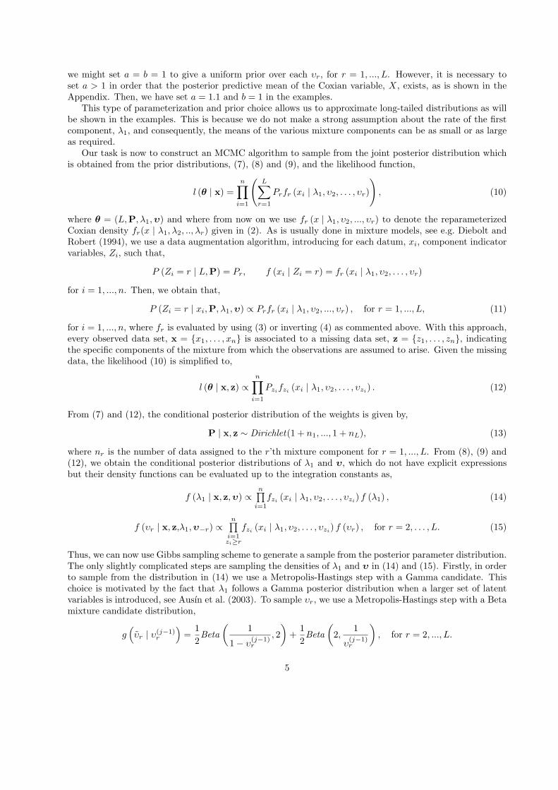
Figure 2: Histograms, predictive densities (solid line) and theoretical densities (dotted line) for the foursimulated data sets. The fits are so close to the true densities that it is sometimes complicated to differentiateboth lines.

2. A Coxian distribution with P = (0.09, 0.7, 0.01, 0.2) and λ = (1.1, 1, 0.251, 0.25) .

3. A Weibull density , f (x) = cacxc−1 exp {− (ax)c}, with (c, a) = (0.3, 9.26053).

4. A Pareto distribution, f (x) = ab (1 + bx)−(a+1), with (a, b) = (2.2, 0.8333).

The exponential distribution is the simplest case of a Coxian distribution. In case 2, we have chosen aCoxian distribution with two pairs of very similar rates to illustrate that this does not affect the stability ofthe algorithm as commented earlier. These two examples are short-tailed distributions. Cases 3 and 4 aretwo of the examples of long tailed distributions considered in Feldman and Whitt (1998). The distributionsin cases 1, 3 and 4 all have means equal to unity.

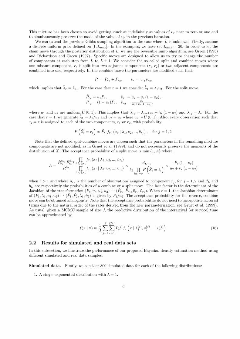
Figure 2 illustrates the empirical and predictive cumulative distribution function estimated after runningthe MCMC algorithm for 10000 burn-in iterations followed by an additional 100000 iterations. We canobserve that the fits are quite satisfactory even for the heavy-tailed cases. The proportions of moves acceptedare 27.2%, 13.13%, 12.88% and 16.85% for the exponential, Coxian, Weibull and Pareto cases, respectively,which are reasonable values in reversible jump setups, see Richardson and Green (1997). Figure 3 showsthe trace plots of the posterior samples of the mixture size, L, for the four simulated data sets, indicatinga good mixing performance. The MCMC algorithm was programmed in FORTRAN and the computationalcost depend mainly on the number of phases required to approximate the distribution, varying from a fewminutes for the exponential distribution to about one hour for the Weibull data.

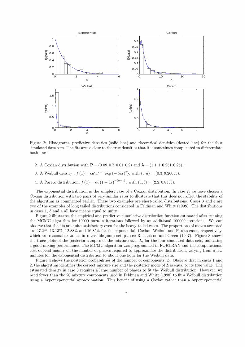
Figure 4 shows the posterior probabilities of the number of components, L. Observe that in cases 1 and2, the algorithm identifies the correct mixture size and the posterior mode of L is equal to its true value. Theestimated density in case 3 requires a large number of phases to fit the Weibull distribution. However, weneed fewer than the 20 mixture components used in Feldman and Whitt (1998) to fit a Weibull distributionusing a hyperexponential approximation. This benefit of using a Coxian rather than a hyperexponential

7

0 2 4 6 8 10

x 104

1

2

3

4

5Exponential

0 2 4 6 8 10

x 104

2

3

4

5

6

7

8Coxian

0 2 4 6 8 10

x 104

8

10

12

14

16

18Weibull

0 2 4 6 8 10

x 104

2

3

4

5

6

7

8Pareto

Figure 3: Trace plots of the MCMC samples from the posterior distribution of the mixture size, L, for thefour simulated data sets. The plots indicate a good mixing performance visiting many different states.

model is further illustrated in case 4 where the posterior mode of L is 3 in contrast with the 14 exponentialcomponents used in Feldman and Whitt (1998).

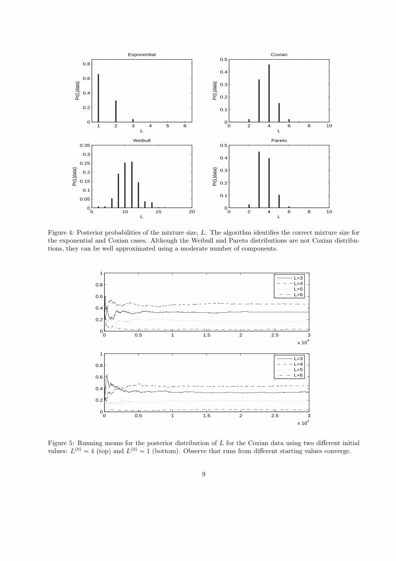
Figure 5 illustrates the running means for the posterior distribution of the mixture size, L, for the Coxiandata set using different starting values in the MCMC algorithm. We can observe that the choice of 10000burn-in iterations seems adequate and that different initial values lead to similar posterior distributions forL.

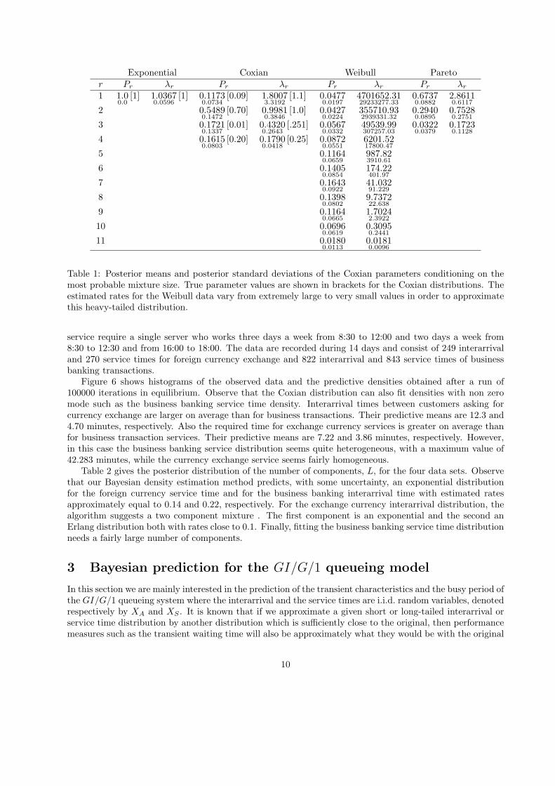
Table 1 shows the posterior means and posterior standard deviations of the parameters conditioning onthe most probable mixture size. For the exponential data set, the most probable model is a single mixturecomponent (see Figure 4) and, conditioning on L = 1, the posterior mean of λ1 is 1.0366, which is very closeto the true rate, 1. For the Coxian data set, the estimated parameters conditioning on the most probablemixture size, L = 4, are in general close to the true values. However, note that although the Coxiandistribution (1) with the order restriction (5) is an identifiable model, very different values of the parametersmay lead to similar density functions. Then, the posterior distributions of various Coxian parameters are notunimodal and the parameters are not significant. Nevertheless, the main interest in practice is the estimationof the density function (see Figure 2) and not the estimation of the parameters. For the Weibull data set,the most probable mixture size is L = 11. Observe that the estimated rates, λr, vary from extremely largeto very small values in order to approximate this heavy-tailed distribution. This is possible because we haveassumed an improper prior distribution for the rates, see (8) and (9). Note that using a proper prior foreach λr as considered in Ausın et al. (2003), the posterior mean of the rates cannot be as small or as largeas required. Finally, Table 1 also shows the estimated parameters for the Pareto data set conditioning onL = 3.

Real data. We now illustrate the method with real interarrival and service times taken from from a face-to-face bank data base available from http://iew3.technion.ac.il/serveng. We consider data of twodifferent kind of services: foreign currency exchange and business banking transactions. These types of

8

1 2 3 4 5 60

0.2

0.4

0.6

0.8

L

Pr(L

|dat

a)

Exponential

0 2 4 6 8 100

0.1

0.2

0.3

0.4

0.5

L

Pr(L

|dat

a)

Coxian

5 10 15 200

0.05

0.1

0.15

0.2

0.25

0.3

0.35

L

Pr(L

|dat

a)

Weibull

0 2 4 6 8 100

0.1

0.2

0.3

0.4

0.5

LPr

(L|d

ata)

Pareto

Figure 4: Posterior probabilities of the mixture size, L. The algorithm identifies the correct mixture size forthe exponential and Coxian cases. Although the Weibull and Pareto distributions are not Coxian distribu-tions, they can be well approximated using a moderate number of components.

0 0.5 1 1.5 2 2.5 3

x 104

0

0.2

0.4

0.6

0.8

1L=3L=4L=5L=6

0 0.5 1 1.5 2 2.5 3

x 104

0

0.2

0.4

0.6

0.8

1L=3L=4L=5L=6

Figure 5: Running means for the posterior distribution of L for the Coxian data using two different initialvalues: L(0) = 4 (top) and L(0) = 1 (bottom). Observe that runs from different starting values converge.

9

Exponential Coxian Weibull Paretor Pr λr Pr λr Pr λr Pr λr

1 1.00.0

[1] 1.03670.0596

[1] 0.11730.0734

[0.09] 1.80073.3192

[1.1] 0.04770.0197

4701652.3129233277.33

0.67370.0882

2.86110.6117

2 0.54890.1472

[0.70] 0.99810.3846

[1.0] 0.04270.0224

355710.932939331.32

0.29400.0895

0.75280.2751

3 0.17210.1337

[0.01] 0.43200.2643

[.251] 0.05670.0332

49539.99307257.03

0.03220.0379

0.17230.1128

4 0.16150.0803

[0.20] 0.17900.0418

[0.25] 0.08720.0551

6201.5217800.47

5 0.11640.0659

987.823910.61

6 0.14050.0854

174.22401.97

7 0.16430.0922

41.03291.229

8 0.13980.0802

9.737222.638

9 0.11640.0665

1.70242.3922

10 0.06960.0619

0.30950.2441

11 0.01800.0113

0.01810.0096

Table 1: Posterior means and posterior standard deviations of the Coxian parameters conditioning on themost probable mixture size. True parameter values are shown in brackets for the Coxian distributions. Theestimated rates for the Weibull data vary from extremely large to very small values in order to approximatethis heavy-tailed distribution.

service require a single server who works three days a week from 8:30 to 12:00 and two days a week from8:30 to 12:30 and from 16:00 to 18:00. The data are recorded during 14 days and consist of 249 interarrivaland 270 service times for foreign currency exchange and 822 interarrival and 843 service times of businessbanking transactions.

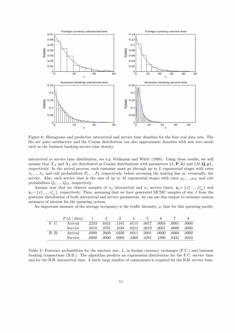
Figure 6 shows histograms of the observed data and the predictive densities obtained after a run of100000 iterations in equilibrium. Observe that the Coxian distribution can also fit densities with non zeromode such as the business banking service time density. Interarrival times between customers asking forcurrency exchange are larger on average than for business transactions. Their predictive means are 12.3 and4.70 minutes, respectively. Also the required time for exchange currency services is greater on average thanfor business transaction services. Their predictive means are 7.22 and 3.86 minutes, respectively. However,in this case the business banking service distribution seems quite heterogeneous, with a maximum value of42.283 minutes, while the currency exchange service seems fairly homogeneous.

Table 2 gives the posterior distribution of the number of components, L, for the four data sets. Observethat our Bayesian density estimation method predicts, with some uncertainty, an exponential distributionfor the foreign currency service time and for the business banking interarrival time with estimated ratesapproximately equal to 0.14 and 0.22, respectively. For the exchange currency interarrival distribution, thealgorithm suggests a two component mixture . The first component is an exponential and the second anErlang distribution both with rates close to 0.1. Finally, fitting the business banking service time distributionneeds a fairly large number of components.

3 Bayesian prediction for the GI/G/1 queueing model

In this section we are mainly interested in the prediction of the transient characteristics and the busy period ofthe GI/G/1 queueing system where the interarrival and the service times are i.i.d. random variables, denotedrespectively by XA and XS . It is known that if we approximate a given short or long-tailed interarrival orservice time distribution by another distribution which is sufficiently close to the original, then performancemeasures such as the transient waiting time will also be approximately what they would be with the original

10

0 20 40 600

0.01

0.02

0.03

0.04

0.05

0.06

0.07

x

f(x|d

ata)

Foreign currency interarrival time

0 10 20 30 40 500

0.02

0.04

0.06

0.08

0.1

0.12

0.14

x

f(x|d

ata)

Foreign currency service time

0 10 20 300

0.05

0.1

0.15

0.2

0.25

x

f(x|d

ata)

Business banking interarrival time

0 10 20 30 400

0.05

0.1

0.15

0.2

0.25

xf(x

|dat

a)

Business banking service time

Figure 6: Histograms and predictive interarrival and service time densities for the four real data sets. Thefits are quite satisfactory and the Coxian distribution can also approximate densities with non zero modesuch as the business banking service time density.

interarrival or service time distribution, see e.g. Feldmann and Whitt (1998). Using these results, we willassume that XA and XS are distributed as Coxian distributions with parameters {L,P, λ} and {M,Q,µ} ,respectively. In the arrival process, each customer must go through up to L exponential stages with ratesλ1, ..., λL and exit probabilities P1, ..., PL respectively, before accessing the waiting line or, eventually, theservice. Also, each service time is the sum of up to M exponential stages with rates µ1, ..., µM and exitprobabilities Q1, ..., QM , respectively.

Assume now that we observe samples of na interarrival and ns service times, xa= {xa1 , ..., xa

na} and

xs= {xs1, ..., x

sns}, respectively. Then, assuming that we have generated MCMC samples of size J from the

posterior distribution of both interarrival and service parameters, we can use this output to estimate variousmeasures of interest for the queueing system.

An important measure of the average occupancy is the traffic intensity, ρ, that for this queueing model,

P (L | data) 1 2 3 4 5 6 7 8F. C. Arrival .2233 .6451 .1181 .0115 .0017 .0003 .0001 .0000

Service .5019 .3701 .1048 .0212 .0019 .0001 .0000 .0000B. B. Arrival .6999 .2669 .0320 .0011 .0001 .0000 .0000 .0000

Service .0000 .0000 .0000 .3369 .4281 .1896 .0431 .0024

Table 2: Posterior probabilities for the mixture size, L, in foreign currency exchanges (F.C.) and businessbanking transactions (B.B.). The algorithm predicts an exponential distribution for the F.C. service timeand for the B.B. interarrival time. A fairly large number of components is required for the B.B. service time.

11

conditional on the system parameters is given by,

ρ =E [XS | M,Q, µ]E [XA | L,P,λ]

=

∑Mr=1Qr

∑rk=1

1µk∑L

r=1Pr

∑rk=1

1λk

. (17)

It is well known that the system is stable if ρ < 1, see e.g. Gross and Harris (1985). The posterior probabilityof having a stable queue can be estimated with,

P (ρ < 1 | xa,xs) ≈ R

J, (18)

where R is the number of times that the value of the traffic intensity calculated from (17) for each element ofthe MCMC sample (L(j),P(j), λ(j),M (j),Q(j), µ(j)) for j = 1, ..., J is less than unity. Note that the posteriormean of ρ is given by,

E [ρ | xa,xs] = E

[M∑

r=1Qr

r∑k=1

1µk

| xs

]× E

[(L∑

r=1Pr

r∑k=1

1λk

)−1

| xa

]. (19)

Given the prior structure used, this is finite as shown in the Appendix. Thus, the expectation can beestimated by the sample mean of the traffic intensities for each element of the MCMC sample. Analogously,we can estimate the posterior mean of ρ assuming stability, E [ρ | ρ < 1,xa,xs].

3.1 Estimation of the transient behaviour and busy period distributions

Bertsimas and Nakazato (1992) obtain closed expressions for the Laplace transform of the busy period, thetransient waiting time and the transient queue length when the system parameters, {L,P,λ} and {M,Q,µ},are known. The estimation procedure described in this section is based on these results.

Bertsimas and Nakazato (1992) show that, conditional on ρ < 1, the Laplace transform of the cumulativedistribution function of the length of a busy period, B, is given by,

∫ ∞

0

e−st Pr (B ≤ t) dt =1s−

1−∑Mr=1Qr

∏rk=1

(µk

µk+s

)

s

M∏r=1

s + µr

s− yr (s)(20)

where yr (s), for r = 1, ..., M , are the M roots of the following equation,[

L∑r=1

Pr

r∏

k=1

(λk

λk + s− yr (s)

)]×

[M∑

t=1

Qt

r∏

k=1

(µk

µk + yr (s)

)]= 1, (21)

with negative real part, for any complex s with positive real part. Bertsimas and Nakazato (1992) demon-strate that given s, equation (21) has M roots of interest, yr (s), for r = 1, ..., M, having negative real partand a further L roots with non negative real part.

The roots of the equation (21) cannot be found analytically and Bertsimas and Nakazato (1992) suggestusing Mathematica to compute them. This approach is not feasible when using reversible jump methods asthe equation is distinct at every MCMC iteration and does not always even have the same number of roots.Therefore, we propose to extract the roots numerically as follows. Note that, given s, the roots yr(s) ofequation (21) are also roots of the following polynomial,

P (yr (s)) =

[L∑

r=1

M∑t=1

PrQt

(r∏

k=1

λk

t∏

k=1

µk

)Qr,t (yr (s))

]−Q0,0 (yr (s)) , (22)

where Qr,t (yr (s)) is another polynomial given by,

Qr,t (yr (s)) =L∏

k=r+1

(λk + s− yr (s))M∏

k=t+1

(µk + yr (s)) ,

12

whose roots are given by {(λr+1 + s) , ..., (λL + s) ,−µt+1, ...,−µM} and the coefficient of order (L+M−r−t)is (−1)L−r. Then, we can apply for example the Laguerre algorithm, see e.g. Ralston and Rabinowitz (1978),which is designed specifically to find the roots of a complex polynomial.

This numerical procedure can be combined with the MCMC algorithm in order to estimate the busyperiod distribution function as follows. Given a sample realization from the posterior distribution of theparameters, (L(j),P(j), λ(j),M (j),Q(j), µ(j)) for j = 1, ..., J , the natural way of estimating the predictivedistributions is using a Monte Carlo approximation,

Pr (B ≤ t | xa,xs, ρ < 1) ≈ 1R

∑

j:ρ(j)<1

Pr(B ≤ t | θ(j)

), (23)

where Pr(B ≤ t | θ(j)) is obtained by numerically inverting the Laplace transform given in (20) for eachelement of the MCMC sample, θ(j). This can be done using a fast numerical, Laplace transform inversionmethod such as that described in Hosono (1981) and extracting numerically the M (j) roots of equation (21)as describe above. The error of numerical inversion of the Hosono algorithm is less than 10−p+1 |f(t)| for anyinverted function f(t), given a previously chosen value p, see also Bertsimas and Nakazato (1992). Then,considering that Pr(B ≤ t | θ(j)) is bounded by one, the error of numerical inversion for this probability isless than 10−p+1 for each t. In our examples, we have chosen p = 6.

Analogously, we can estimate the distribution function of the transient waiting time and the transientqueue length distributions functions using the two following results. Assuming that the system is initiallyempty and some other mild initial conditions, Bertsimas and Nakazato (1992) show that if ρ < 1, the Laplacetransform of the waiting time, W (τ) , of a customer arriving at time τ is given by,

∫ ∞

0

e−sτ Pr (W (τ) ≤ w) dτ =1s

+M∑

r=1

(−1)Meyr(s)w

s

M∏k=1

µk + yr(s)µk

M∏k=1k 6=r

yk(s)yr(s)− yk(s)

, (24)

where yr (s), for r = 1, ..., M , are the M roots of equation (21) with negative real part.And finally, assuming the same initial conditions, Bertsimas and Nakazato (1992) give a expression for

the Laplace transform of the number of customers, N (τ) , in the system at time τ,

∫ ∞

0

e−sτ Pr (N (τ) = n) dτ =

{ ∑Li=1 π∗0,i (s) , if n = 0,∑L

i=1

∑Mj=1 π∗n,i,j (s) , if n ≥ 1,

(25)

where π∗0,i (s) is the Laplace transform of the probability that at time τ the number of customers in thesystem is 0 and the arrival stage currently occupied by the arriving customer is i, and π∗n,i,j (s) is the Laplacetransform of the probability that at time τ the number of customers in the system is n, the arrival stagecurrently occupied by the arriving customer is i, and the service who is being served is j. The expressionsfor π∗0,i (s) and π∗n,i,j (s) are more complicated and are not reported here to save space, although they canbe numerically evaluated without difficulties. These depend again on the roots of equation (21).

It can be shown that the predictive moments of the system size and waiting time in equilibrium, i.e.when τ →∞, and the moments of the busy period distribution do not exist given any prior formulation thatplaces positive mass on ρ = 1, see e.g. Wiper (1998). Thus, the moments of the transient distributions willgo to infinity as τ goes to infinity. However, as alternatives, we can calculate the median and quantiles ofthese distributions.

3.2 Results for simulated and real queues

In this section, we illustrate the behaviour of the proposed method with several simulated and real queuesbased on the data sets analysed in Section 2. Firstly we consider two simulated queueing systems and thenreal systems in the Israeli bank.

13

Simulated data. We use interarrival and service data simulated from the following two queueing systemswith approximately the same traffic intensity ρ = 0.289.

• An M/M/1 system where the service times are the exponential data simulated in Section 2 and 300arrival times were simulated from an exponential distribution with mean 3.456.

• A Coxian/Pareto/1 system where both interarrival and service time data are as in Section 2.

Table 3 shows the probabilities of equilibrium in the system and the posterior means of ρ for both systems.Also shown are the MLE estimates of ρ. As we might expect, the estimates are very close to the true value.

P (ρ < 1 | data) E [ρ | data] E [ρ | ρ < 1, data] ρMLE

M/M/1 .99998 .29009 .29008 .28935Coxian/Pareto/1 .99993 .30740 .30736 .28116

Table 3: Posterior probabilities that the system is stable and posterior mean values and MLE estimates forthe traffic intensity for the two simulated systems. The equilibrium probability is extremely large in bothcases and the estimations of ρ are very close to the true value.

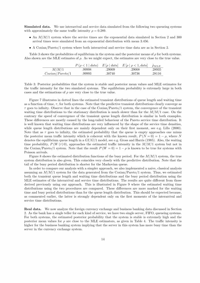
Figure 7 illustrates in dotted lines the estimated transient distributions of queue length and waiting timeas a function of time, τ , for both systems. Note that the predictive transient distributions clearly converge asτ goes to infinity. Observe that in the case of the Coxian/Pareto/1 system, the convergence of the transientwaiting time distributions to the stationary distribution is much slower than for the M/M/1 case. On thecontrary the speed of convergence of the transient queue length distribution is similar in both examples.These differences are mostly caused by the long-tailed behaviour of the Pareto service time distribution. Itis well known that waiting time distributions are very influenced by the shape of the service time densities,while queue length distributions are mainly dependent only on their first moment, see e.g. Lillo (2000).Note that as τ goes to infinity, the estimated probability that the queue is empty approaches one minusthe posterior mean traffic intensity which is coherent with the known result, P (N = 0) = 1 − ρ, where Ndenotes the equilibrium queue length in a GI/G/1 model, see e.g. Gross and Harris (1985). Also, the waitingtime probability, P (W (τ) 0), approaches the estimated traffic intensity in the M/M/1 system but not inthe Coxian/Pareto/1 system. Note that the result P (W = 0) = 1− ρ is known to be true for systems withPoisson arrivals.

Figure 8 shows the estimated distribution functions of the busy period. For the M/M/1 system, the truesystem distribution is also given. This coincides very closely with the predictive distribution. Note that thetail of the busy period distribution is shorter for the Markovian queue.

In order to compare our analysis with a simpler approach, we also implemented a naive, classical analysisassuming an M/M/1 system for the data generated from the Coxian/Pareto/1 system. Thus, we estimatedboth the transient queue length and waiting time distributions and the busy period distribution using theMLE estimates of the interarrival and service time distributions. The results are quite different from thosederived previously using our approach. This is illustrated in Figure 9 where the estimated waiting timedistributions using the two procedures are compared. These differences are more marked for the waitingtime and busy period distributions than for the queue length distribution. This should be expected because,as commented earlier, the latter is strongly dependent only on the first moments of the interarrival andservice time distributions.

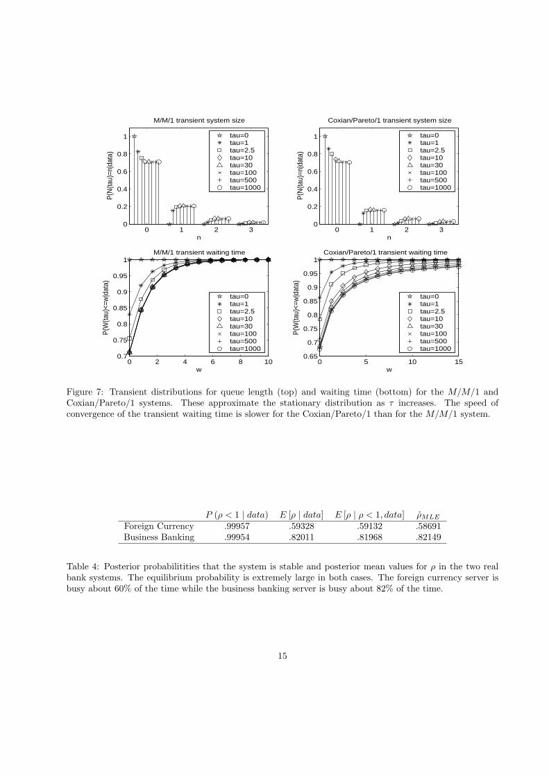
Real data. We now analyze the foreign currency exchange and business banking data discussed in Section2. As the bank has a single teller for each kind of service, we have two single server, FIFO, queueing systems.For both systems, the estimated posterior probability that the system is stable is extremely high and theposterior mean values for ρ are close to the MLE estimators, as given in Table 4. The traffic intensity ishigher for the business banking system implying that the server in this system has more busy time than theserver in the currency exchange system.

14

0 1 2 30

0.2

0.4

0.6

0.8

1

n

P(N

(tau)

=n|d

ata)

M/M/1 transient system size

tau=0tau=1tau=2.5tau=10tau=30tau=100tau=500tau=1000

0 1 2 30

0.2

0.4

0.6

0.8

1

n

P(N

(tau)

=n|d

ata)

Coxian/Pareto/1 transient system size

tau=0tau=1tau=2.5tau=10tau=30tau=100tau=500tau=1000

0 2 4 6 8 100.7

0.75

0.8

0.85

0.9

0.95

1

w

P(W

(tau)

<=w

|dat

a)

M/M/1 transient waiting time

tau=0tau=1tau=2.5tau=10tau=30tau=100tau=500tau=1000

0 5 10 150.65

0.7

0.75

0.8

0.85

0.9

0.95

1

w

P(W

(tau)

<=w

|dat

a)

Coxian/Pareto/1 transient waiting time

tau=0tau=1tau=2.5tau=10tau=30tau=100tau=500tau=1000

Figure 7: Transient distributions for queue length (top) and waiting time (bottom) for the M/M/1 andCoxian/Pareto/1 systems. These approximate the stationary distribution as τ increases. The speed ofconvergence of the transient waiting time is slower for the Coxian/Pareto/1 than for the M/M/1 system.

P (ρ < 1 | data) E [ρ | data] E [ρ | ρ < 1, data] ρMLE

Foreign Currency .99957 .59328 .59132 .58691Business Banking .99954 .82011 .81968 .82149

Table 4: Posterior probabilitities that the system is stable and posterior mean values for ρ in the two realbank systems. The equilibrium probability is extremely large in both cases. The foreign currency server isbusy about 60% of the time while the business banking server is busy about 82% of the time.

15

0 2 4 6 8 10 12 14 16 18 200

0.1

0.2

0.3

0.4

0.5

0.6

0.7

0.8

0.9

1

x

FB(x

|dat

a)

Busy period distribution functions for the simulated queues

estimated M/M/1 busy period cdftrue M/M/1 busy period cdfestimated Coxian/Pareto/1 busy period cdf

Figure 8: Estimated busy period distribution functions for the M/M/1 and Coxian/Pareto/1 systems. Thetrue distribution for the M/M/1 system is also plotted and is very close to the estimated distribution. Thetail of the busy period distribution is shorter for the M/M/1 queue.

0 5 10 150.65

0.7

0.75

0.8

0.85

0.9

0.95

1

w

P(W

(tau)

<=w

|dat

a)

Coxian/Pareto/1 transient waiting time

tau=0tau=1tau=2.5tau=10tau=30tau=100tau=500tau=1000

Figure 9: Estimated transient waiting time distribution using the proposed Bayesian GI/G/1 model (solidlines) and a simple MLE estimation based on a M/M/1 system (dotted lines) for the data generated fromthe Coxian/Pareto/1 system. The results are rather different using both approaches.

16

0 1 2 30

0.2

0.4

0.6

0.8

1

n

P(N

(tau)

=n|d

ata)

Foreign currency transient system size

tau=0tau=1tau=2.5tau=10tau=30tau=100tau=500tau=1000

0 1 2 30

0.2

0.4

0.6

0.8

1

n

P(N

(tau)

=n|d

ata)

Business banking transient system size

tau=0tau=1tau=2.5tau=10tau=30tau=100tau=500tau=1000

0 10 20 30 40 500.4

0.5

0.6

0.7

0.8

0.9

1

w

P(W

(tau)

<=w

|dat

a)

Foreign currency transient waiting time

tau=0tau=1tau=2.5tau=10tau=30tau=100tau=500tau=1000

0 10 20 30 40 500

0.2

0.4

0.6

0.8

1

w

P(W

(tau)

<=w

|dat

a)

Business banking transient waiting time

tau=0tau=1tau=2.5tau=10tau=30tau=100tau=500tau=1000

Figure 10: Predictive transient queue length (top) and waiting time (down) distributions for the banksystems. These approximate the stationary distributions as τ increases but the speed of convergence is slow.For the business banking system, there are still differences between the waiting time distributions after 500and 1000 minutes.

Figure 10 illustrates the estimated distributions of the transient queue length and waiting time for bothsystems as a function of the time, τ . The assumption that the systems are empty at time τ = 0 is true in thiscase. We observe that the speed of convergence is slow in both cases. After τ = 100 minutes, the transientdistributions have still not converged to the steady-state. In particular, for the business banking system, wecan still appreciate differences between the waiting time distributions after 500 and 1000 minutes. Observethat using our approach it is possible to estimate the desired waiting time distribution for a client arrivingat any given instant of time, τ . For example, the estimated probability that a customer who arrives at 9amasking for business banking services has to wait more than 8 minutes is approximately 0.3.

Table 5 shows some quantiles of the estimated distributions of the length of the busy period. Observethat the tail of the distribution is heavier for the business bank transactions case.

0.25 0.50 0.65 0.80 0.90 0.95 0.97Foreign Currency 2.342 6.323 10.902 21.271 41.108 69.610 96.298Business Banking 2.113 4.596 8.411 19.452 46.671 95.431 148.290

Table 5: Quantiles of the busy period distribution for the two bank systems. The tail of the distribution isheavier for the business bank transactions case.

The algorithm used to estimate the transient and busy period distributions was programmed in FOR-

17

0 50 100 150 200 2500

5

10

15

20

25

τ

W(τ

)

50% quantile80% quantile

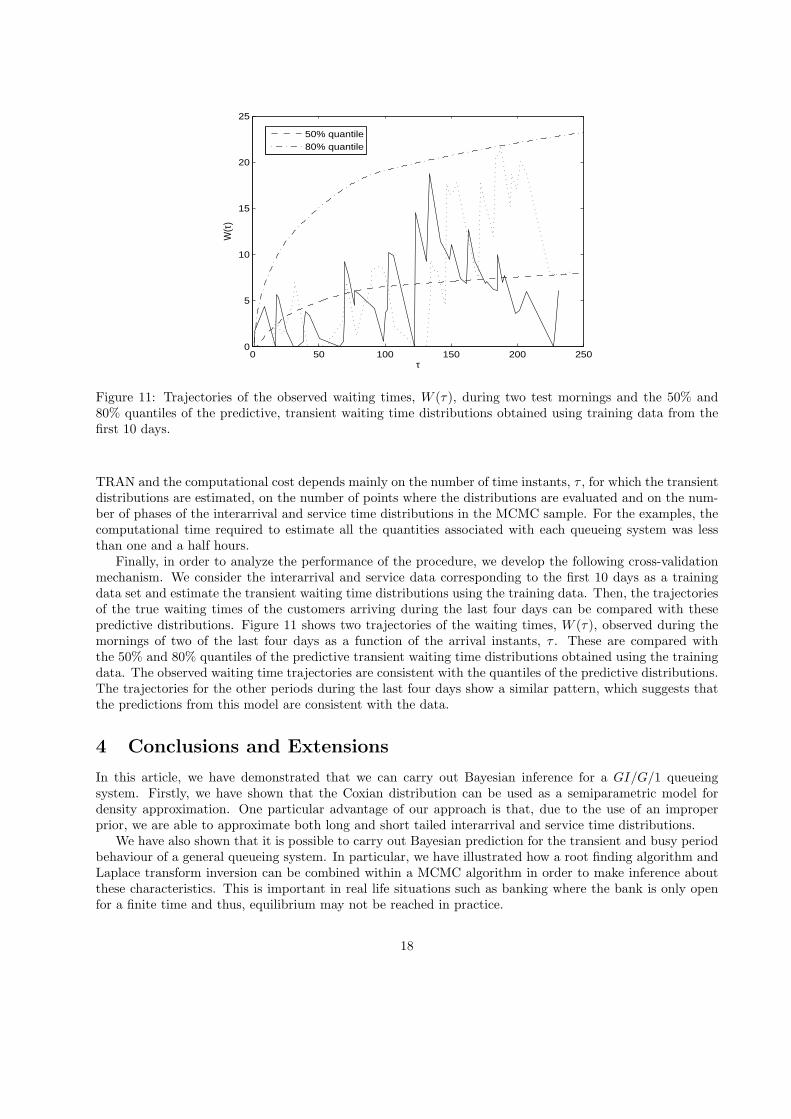
Figure 11: Trajectories of the observed waiting times, W (τ), during two test mornings and the 50% and80% quantiles of the predictive, transient waiting time distributions obtained using training data from thefirst 10 days.

TRAN and the computational cost depends mainly on the number of time instants, τ , for which the transientdistributions are estimated, on the number of points where the distributions are evaluated and on the num-ber of phases of the interarrival and service time distributions in the MCMC sample. For the examples, thecomputational time required to estimate all the quantities associated with each queueing system was lessthan one and a half hours.

Finally, in order to analyze the performance of the procedure, we develop the following cross-validationmechanism. We consider the interarrival and service data corresponding to the first 10 days as a trainingdata set and estimate the transient waiting time distributions using the training data. Then, the trajectoriesof the true waiting times of the customers arriving during the last four days can be compared with thesepredictive distributions. Figure 11 shows two trajectories of the waiting times, W (τ), observed during themornings of two of the last four days as a function of the arrival instants, τ . These are compared withthe 50% and 80% quantiles of the predictive transient waiting time distributions obtained using the trainingdata. The observed waiting time trajectories are consistent with the quantiles of the predictive distributions.The trajectories for the other periods during the last four days show a similar pattern, which suggests thatthe predictions from this model are consistent with the data.

4 Conclusions and Extensions

In this article, we have demonstrated that we can carry out Bayesian inference for a GI/G/1 queueingsystem. Firstly, we have shown that the Coxian distribution can be used as a semiparametric model fordensity approximation. One particular advantage of our approach is that, due to the use of an improperprior, we are able to approximate both long and short tailed interarrival and service time distributions.

We have also shown that it is possible to carry out Bayesian prediction for the transient and busy periodbehaviour of a general queueing system. In particular, we have illustrated how a root finding algorithm andLaplace transform inversion can be combined within a MCMC algorithm in order to make inference aboutthese characteristics. This is important in real life situations such as banking where the bank is only openfor a finite time and thus, equilibrium may not be reached in practice.

18

A number of extensions are possible. Firstly, we should note that to capture multimodal distributions, aCoxian distribution with a large number of phases and hence a large number of parameters is needed. Thiscan make the semiparametric approximation somewhat inefficient. In such cases alternative approximationswhich better capture multimodality could be considered. A difficulty is that in the queueing context, resultsconcerning the transient and busy period behaviour are hard to obtain with such systems.

As pointed out by a referee, in order to attempt to simplify the inferential procedure, we might usemodel selection criteria, such as the Akaike Information Criterion, Bayesian Information Criterion or Bayesfactors, for choosing a single queueing model from the Coxian class. An advantage of this approach is thatonce we have chosen the most probable model for the interarrival and service times, the computation of theperformance measures of the queueing system is simplified.

In this article we have only considered a single server queueing system. From the point of view ofinference for the interarrival and service processes, considering a multi server system presents no extraproblems. However there are more difficulties in estimating the characteristics of the queueing system suchas waiting time as the queueing theory for the Coxian/Coxian/c system is less well developed. Some resultsare available however, see e.g. Bertsimas (1990). Also, we should note that the Coxian distribution is phasetype, see e.g. Neuts (1981) and, for example results for the waiting time in steady state of a system withphase type arrivals and services are known, see e.g. Asmussen et al. (2001).

Another important objective in the queueing context is optimal control of the system, e.g. when to openand close the system or optimizing the number of servers. The methods of Bayesian decision theory can becombined with Bayesian inference to do this. For one example of the use of Bayesian methods to control thecapacity of a queueing system, see e.g. Ausın et al. (2003).

Finally, a further extension is to apply the Coxian model and prior structure in areas such as insurancerisk where long tailed samples are common. In particular, in the context of estimating ruin probabilities,many results from queueing theory can be applied, see e.g. Prabhu (1998). Work is currently underway inthis area.

Acknowledgment

We would like to thank three anonymous referees and editor for their valuable comments and suggestions.We also wish to thank Professor Avi Mandelbaum for allowing us to use the real data from his web page. Weacknowledge the financial support provided by the projects SEJ2004-03303 and 06/HSE/0181/2004. Thefirst author also acknowledges the financial support provided by Xunta de Galicia under the Isidro PargaPondal Program.

Appendix: Proof that the posterior of ρ is proper with finite mean

Here, we show that the posterior is indeed proper. Assume that we observe a sample x1, ..., xn from aCoxian random variable X with parameters θ = (L,P, λ1,υ) and that we use the prior distribution definedin Section 2. Then, we need to prove that the following integral is finite,

∫f (θ)

n∏

i=1

(L∑

r=1Prfr (xi | λ1,υ)

)dθ. (26)

Let us denote, for r = 1, ..., L,

Cj,r =r∏

i6=j

λi

λi − λj=

r∏

i 6=j

∏ik=2υk∏i

k=2υk −∏j

k=2υk

, for j = 1, ..., r.

19

Observe that∑r

j=1Cj,r = 1, see e.g. McGill et al. (1965). Then, for n = 1, the integral (26) is given by,

∫f (L) f (P|L) f (υ|L)

λ1

L∑r=1

Pr

r∑j=1

Cj,rλ1

j∏k=2

υk exp(−λ1x1

j∏k=2

υk

)dθ

=1x

∫f (L) f (P|L) f (υ|L)

L∑r=1

Pr

r∑j=1

Cj,rdθ−λ1 =1x

< ∞,

where we have denoted θ−λ1 = (L,P,υ) . Finally, note that it is sufficient to have proved that the integral(26) is finite for n = 1, because now, we can define f (θ | x1) as a new proper prior and consider the likelihoodbased on {x2, ..., xn}, which is regular and proper, in which case the posterior is known to be proper. Then,the integral (26) is finite for n ≥ 1.

Now, we will prove that the posterior mean of ρ given in (19) is finite. Firstly, observe that the generalizedErlang distribution, whose density is given in (27), is bounded by the first rate,

fr (x | λ1, υ) ≤ λ1, (27)

This can be proved by induction. For r = 1, we have that f1 (x | λ1) = λ1e−λ1x ≤ λ1. Now, for i = 2, ..., r−1

assume that,fi (x | λ1, υ) = fi (x | λ1, ..., λi) ≤ λ1,

where λi = λ1υ2..., υr. Then, as fr is the density of the sum of r exponentials, it can be expressed as theconvolution of the r’th exponential density and fr−1, that is,

fr (x | λ1, ..., λr) =∫ x

0

λr exp (−λrx) fr−1 (x− u | λ1, ..., λr−1) du

≤ λ1 [1− exp {−λrx}] ≤ λ1.

Using this property, we now prove that the first factor of (19), which is the predictive mean of the Coxiandistribution, is finite. It is clear that if we do not observe at least two data the predictive mean does notexit. Then, assuming that xs = {xs

1, xs2} and using (27),

E

[M∑

r=1Qr

r∑j=1

1µj|xs

]∝

∫M∑

r=1Qr

r∑j=1

f (θ)

µ1

∏jk=2υk

2∏

i=1

(M∑

r=1Qrfr (xi | µ1,υ)

)dθ

≤∫ (

M∑r=1

Qr

r∑j=1

f (θ)∏jk=2υk

)(M∑

r=1Qrfr (x1 | µ1,υ)

)dθ

=∫ (

M∑r=1

Qr

r∑j=1

f (M) f (Q|M) f (υ|M)∏jk=2υk

)(M∑

r=1Qr

r∑j=1

Cj,r

j∏k=2

υk exp(−µ1x1

j∏k=2

υk

))dθ

=1x1

∫M∑

r=1Qr

r∑j=1

f (M) f (Q|M) f (υ|M)∏jk=2υk

dθ−µ1

=1x1

∫M∑

r=1Qr

r∑j=1

f (M) f (Q|M) dQ∫

f (υ|M)∏jk=2υk

dυ

≤ ∞ if a > 1.

Finally, as this integral is finite for n = 2, we can define a new proper prior for θ,

g (θ) ∝M∑

r=1Qr

r∑j=1

f (θ)µ1

∏rk=2υk

2∏

i=1

(M∑

r=1Qrfr (xi | µ1, υ)

),

which is a proper density. With this prior and the likelihood based on {x3, ..., xn} , the posterior is properand then, the predictive mean is finite for n ≥ 2.

20

Finally, let us prove that the second factor of the posterior mean of ρ given in (19) is finite. Firstly, weshow that ,

r∑k=1

1∏rk=2υk

=r∑

j=1

Cj,r∏rk=2υk

.

This can be proved observing that the expectation of a generalized Erlang, fr, which is a sum of r exponentialrandom variables with rates λ1, ..., λr, is given by the sum of the inverse of these rates,

r∑

j=1

1λj

=r∑

k=1

1λ1

∏rk=2υk

=∫ ∞

0

xr∑

j=1

Cj,rλ1

r∏k=2

υk exp(−λ1x1

r∏k=2

υk

)dx =

r∑j=1

Cj,r

λ1

∏rk=2υk

.

We now assume that na = 1,

E

(L∑

r=1Pr

r∑j=1

1λj

)−1

|xa

∝

∫f (θ)

L∑r=1

Pr

r∑j=1

(λ1

∏jk=2υk

)−1

(L∑

r=1Prfr (x1 | λ1, υ)

)dθ

=∫

f (L) f (P|L) f (υ|L)L∑

r=1Pr

r∑j=1

(∏jk=2υk

)−1

(L∑

r=1Prfr (x1 | λ1, υ)

)dθ

=∫

f (L) f (P|L) f (υ|L)L∑

r=1Pr

r∑j=1

(∏jk=2υk

)−1

L∑r=1

Pr

r∑j=1

Cj,rλ1

j∏k=2

υk exp(−λ1x1

j∏k=2

υk

)dθ

=1x2

1

∫f (L) f (P|L) f (υ|L)L∑

r=1Pr

r∑j=1

(∏jk=2υk

)−1

L∑r=1

Pr

r∑j=1

Cj,r∏jk=2υk

dθ

=1x2

1

∫f (L) f (P|L) f (υ|L)L∑

r=1Pr

r∑j=1

(∏jk=2υk

)−1

L∑r=1

Pr

r∑j=1

(∏jk=2υk

)−1

dθ−λ1

=1x2

1

∫f (L) f (P|L) f (υ|L) dθ−λ1 =

1x2

1

Now, using the same arguments as above, this integral is also finite for na ≥ 1 .

References

Abate, J., Choudhury, G. L., and Whitt, W. (1994). Waiting-time tail probabilities in queues with long-tailservice-time distributions. Queueing Systems. 16, 311-338.

Armero, C., and Bayarri, M.J., 1994. Bayesian prediction in M/M/1 queues. Queueing Systems. 15,401-417.

Armero, C., and Bayarri, M. J. 1997. Bayesian analysis of a queueing system with unlimited service.Journal of Statistical Planning and Inference. 58, 241-261.

Armero, C., and Conesa, D. 2000. Prediction in Markovian bulk arrival queues. Queueing Systems. 34,327-350.

Asmussen, S., and Moller, J.R., 2001. Calculation of the steady-state waiting time distribution in GI/PH/cand MAP/PH/c queues. Queueing Systems. 37, 9-29.

21

Ausın, M.C., Lillo, R.E., Ruggeri, F., and Wiper, M.P. 2003. Bayesian modelling of hospital bed occupancytimes using a mixed generalized Erlang distribution. In: J.M. Bernardo, M.J. Bayarri, J.O. Berger,A.P. Dawid, D. Heckerman, A.F.M. Smith and M. West (Ed.),Bayesian Statistics 7, Oxford UniversityPress, Oxford, 443-452.

Ausın, M.C., Wiper, M.P., and Lillo, R.E., 2004. Bayesian estimation for the M/G/1 queue using a phasetype approximation, Journal of Statistical Planning and Inference. 118, 83-101.

Bertsimas, D., 1990. An analytic approach to a general class of G/G/c queueing systems. OperationsResearch. 38, 139-155.

Bertsimas, D., and Nakazato, D. 1992. Transient and busy period analysis of the G/G/1 queue: Themethod of stages. Queueing Systems. 10, 153-184.

Crovella, M. E., Taqqu, M.S., and Bestavros, A. 1998. Heavy-Tailed Probability Distributions in the WorldWide Web. In: R.J. Adler, R.E. Feldman and M.S. Taqqu (Ed.), A Practical Guide To Heavy Tails,Chapman and Hall, New York, 3-26.

Cox, D. R. 1955. A use of complex probabilities in the theory of stochastic processes. Proc. Cam. Phil.Soc. 51, 313319.

Cumani, A., 1982. On the canonical representation of homogenous Markov processes modelling failure-timedistributions. Microelectronics and reliability. 22, 583-602.

Diebolt, J., and Robert, C.P., 1994. Estimation of finite mixture distributions through Bayesian sampling.Journal of the Royal Statistical Society, B. 56, 363-375.

Feldmann, A., and Whitt, W. 1998. Fitting mixtures of exponentials to long-tail distributions to analyzenetwork performance models. Performance Evaluation. 31, 245-279.

Green, P. 1995. Reversible jump MCMC computation and Bayesian model determination. Biometrika. 82,711-732.

Gross, D., and Harris, C.M., 1985. Fundamentals of queueing theory. John Wiley & Sons, New York.

Gruet, M.A., Philippe, A., and Robert, C.P., 1999. MCMC control spreadsheets for exponential mixtureestimation. Journal of Computational and Graphical Statistics. 8, 298-317.

Hosono, T., 1981. Numerical inversion of Laplace transform and some applications to wave optics. RadioScience. 16, 1015-1019.

Johnson, N.L., and Kotz, S., 1970. Distributions in statistics. Continuous univariate distributions. JohnWiley & Sons, New York.

Lillo, R., 2000. On the optimal control of M/G/1 systems under the cycle criterion. Systems and ControlLetters. 41, 29-39.

McGill, W. J., and Gibbon, J., 1965. The general-gamma distribution and reaction time. Journal ofMathematical Psychology. 2, 1-18.

Neuts, M.F., 1981. Matrix Geometric Solutions in Stochastic Models. Johns Hopkins University Press,Baltimore.

Paxson, V. and Floyd, S., 1995. Wide-area traffic: The failure of Poisson modeling. IEEE Transactions inNetworking. 3, 226-244.

Prabhu, N.U., 1998. Stochastic Storage Processes, Springer Verlag, New York.

22

Ralston, A., and Rabinowitz, P., 1978. A first course in numerical analysis. McGraw-Hill, New York.

Richardson, S., Green, P. 1997. On Bayesian analysis of mixtures with an unknown number of components.Journal of the Royal Statistical Society, B. 59, 731-792.

Rios, D., Wiper, M.P., and Ruggeri, F., 1998. Bayesian analysis of M/Er/1 and M/Hk/1 queues. QueueingSystems, 30, 289-308.

Riska, A. Diev, V., and Smirni, E., 2004. An EM-based technique for approximating long-tailed data setswith PH distributions. Performance Evaluation, 55, 147-164.

Robert, C.P., and Mengersen, K.L., 1999. Reparameterisation Issues in Mixture Modelling and their bearingon MCMC algorithms. Computational Statistics & Data Analysis, 29, 325-343.

Wiper, M.P., 1998. Bayesian analysis of Er/M/1 and Er/M/c queues. Journal of Statistical Planning andInference, 69, 65-79.

23