Bayesian neural network learning for repeat purchase modelling in direct marketing

KATHOLIEKE UNIVERSITEIT

lEUVEN

DEPARTEMENT TOEGEPASTE ECONOMISCHE WETENSCHAPPEN

RESEARCH REPORT 0114 BAYESIAN NEURAL NETWORK LEARNING FOR

REPEAT PURCHASE MODELLING IN DIRECT MARKETING

by S. VIAENE

B. BAESENS D. VAN DEN POEL J. VANTHIENEN

G.DEDENE

0/2001/2376/14

Bayesian neurai network learning for repeat

purchase modelling in direct marketing

Stijn Viaene1, Bart Baesensl, Dirk Van den Poel2, Jan Vanthienen\ Guido Dedene1

lK.U.Leuven, Dept. of Applied Economic Sciences, Naamsestraat 69, B-3000 Leuven, Belgium

{Stijn.Viaene; Bart.Baesens; Jan.Vanthienen; Guido.Dedene }@econ.kuleuven.ac.be

2Ghent University, Dept. of Marketing, Hoveniersberg 24, B-9000 Ghent, Belgium

[email protected]

Accepted for publication in the European Journal of Operational Research.

Abstract. We focus on purchase incidence modelling for a European direct mail company. Response models based on statistical and neural network techniques are contrasted. The evidence framework of MacKay is used as an example implementa­tion of Bayesian neural network learning, a method that is fairly robust with respect to problems typically encountered when implementing neural networks. The automatic relevance determination (ARD) method, an integrated feature of this framework, al­lows to assess the relative importance of the inputs. The basic response models use operationalisations of the traditionally discussed Recency, Frequency and Monetary (RFM) predictor categories. In a second experiment, the RFM response framework is enriched by the inclusion of other (non-RFM) customer profiling predictors. We contribute to the literature by providing experimental evidence that: (1) Bayesian neural networks offer a viable alternative for purchase incidence modelling; (2) a com­bined use of all three RFM predictor categories is advocated by the ARD method; (3) the inclusion of non-RFM variables allows to significantly augment the predictive power of the constructed RFM classifiers; (4) this rise is mainly attributed to the in­clusion of customer/company interaction variables and a variable measuring whether a customer uses the credit facilities of the direct mailing company.

Keywords: Neural networks, Marketing, Bayesian learning, Response modelling, In­put ranking

1

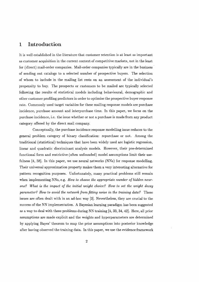
1 Introd uction

It is well established in the literature that customer retention is at least as important

as customer acquisition in the current context of competitive markets, not in the least

for (direct) mail-order companies. Mail-order companies typically are in the business

of sending out catalogs to a selected number of prospective buyers. The selection

of whom to include in the mailing list rests on an assessment of the individual's

propensity to buy. The prospects or customers to be mailed are typically selected

following the results of statistical models including behavioural, demographic and

other customer profiling predictors in order to optimise the prospective buyer response

rate. Commonly used target variables for these mailing response models are purchase

incidence, purchase amount and interpurchase time. In this paper, we focus on the

purchase incidence, i.e. the issue whether or not a purchase is made from any product

category offered by the direct mail company.

Conceptually, the purchase incidence response modelling issue reduces to the

general problem category of binary classification: repurchase or not. Among the

traditional (statistical) techniques that have been widely used are logistic regression,

linear and quadratic discriminant analysis models. However, their pre-determined

functional form and restrictive (often unfounded) model assumptions limit their use­

fulness [4, 58]. In this paper, we use neural networks (NNs) for response modelling.

Their universal approximation property makes them a very interesting alternative for

pattern recognition purposes. Unfortunately, many practical problems still remain

when implementing NNs, e.g. How to choose the appropriate number of hidden neur­

ons'? What is the impact of the initial weight choice'? How to set the weight decay

parameter'? How to avoid the network from fitting noise in the training data'? These

issues are often dealt with in an ad-hoc way [3]. Nevertheless, they are crucial to the

success of the NN implementation. A Bayesian learJ?ing paradigm has been suggested

as a way to deal with these problems during NN training [4,33,34,42]. Here, all prior

assumptions are made explicit and the weights and hyperparameters are determined

by applying Bayes' theorem to map the prior assumptions into posterior knowledge

after having observed the training data. In this paper, we use the evidence framework

2

of MacKay as an example implementation of Bayesian learning [33,34, 35, 36]. An

interesting additional feature of this framework is the automatic relevance determ-

ination (.{d.l.RD) method vvhich allows to assess the relative importance of the various

inputs by adding weight regularisation terms to the objective function. In this paper,.

it is shown that training NNs using the evidence framework (with the ARD exten­

sion) is an effective and viable alternative for the response modelling case at hand

when compared to the three benchmark statistical techniques mentioned above.

The empirical study consists of two subexperiments. Initially, only stand­

ard Recency, Frequency and Monetary (RFM) predictor categories will underly the

purchase incidence model. This choice is motivated by the fact that most previous

research cites them as being most important and because they are internally avail­

able at very low cost [1, 15, 29]. It is shown for this case that, from a predictive

performance perspective, Bayesian NNs are statistically superior when compared to

logistic regression, linear and quadratic discriminant analysis classifiers. Predictive

performance is quantified by means of the percentage correctly classified (PCC) and

the area under the receiver operating characteristic curve (AUROC). The latter ba­

sically illustrates the behaviour of a classifier without regard to class distribution

or error cost, so it effectively decouples classification performance from these factors

[20, 59, 60]. The ARD method is used to shed light upon the relative importance

of all variables operationalising the RFM response model. In a second experiment,

the response model is extended with other potentially interesting customer profiling

variables. It is illustrated that the Bayesian NNs still perform significantly better

than the three statistical classifiers. Again, the relative importance of the inputs is

assessed using the ARD method.

This paper is organised as follows. In Section 2 we provide a concise overview

of response modelling issues in the context of direct marketing. Section 3 discusses

the theoretical underpinnings of NNs for pattern recognition purposes. The Bayesian

evidence framework for classification is presented in Section 4. Section 5 presents the

ARD extension of the evidence framework. The design of the study, including data

set description, experimental setup and used performance criteria are presented in

3

Section 6. Results and discussion of the basic and extended RFM experiment are

covered in Sections 7 and 8.

2 Response modelling in direct marketing

For mail-order response modelling, several alternative problem formulations have

been proposed based on the choice of the dependent variable. The first category is

purchase incidence modelling [9]. In this problem formulation, the main question is

whether a customer will purchase during the next mailing period, i.e. one tries to

predict the purchase incidence within a fixed time interval (typically half a year).

Other authors have investigated related problems dealing with both the purchase

incidence and the amount of purchase in a joint model [32, 64]. A third alternative

perspective for response modelling is to model interpurchase time through survival

analysis or (split-)hazard rate models which model whether a purchase takes place

together with the duration of time until a purchase occurs [16, 63].

This paper focuses on the first type of problem, i.e. purchase incidence

modelling. More specifically, we. consider the issue whether or not a purchase is

made from any product category offered by the direct mail company. This choice is

motivated by the fact that the majority of previous research in the direct marketing

literature focuses on the purchase incidence problem [41, 69]. Furthermore, this is

exactly the setting that mail-order companies are typically confronted with. They

have to decide whether or not a specific offering will be sent to a (potential) customer

during a certain mailing period.

Cullinan is generally credited for identifying the three sets of variables most

often used in response modelling: (R)ecency, (F)requency and (M)onetary [1, 15,29].

Since then, the literature has accumulated so many uses of these three variable cat­

egories, that there is overwhelming evidence both from academically reviewed studies

as well as from practitioners' experience that the RFM variables are an important

set of predictors for modelling mail-order repeat purchasing. However, the beneficial

effect of including other variables into the response model has also been investigated.

4

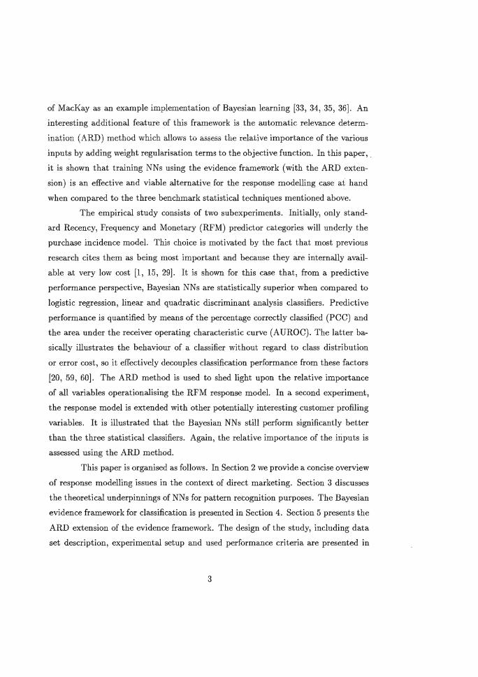
In Table 1, we present a literature overview of the operationalisations of both the in­

dependent and dependent variable( s) in direct marketing response modelling studies.

It shows that only few studies include non-RFM variables. Moreover, these studies

typically include only one operationalisation per variable.

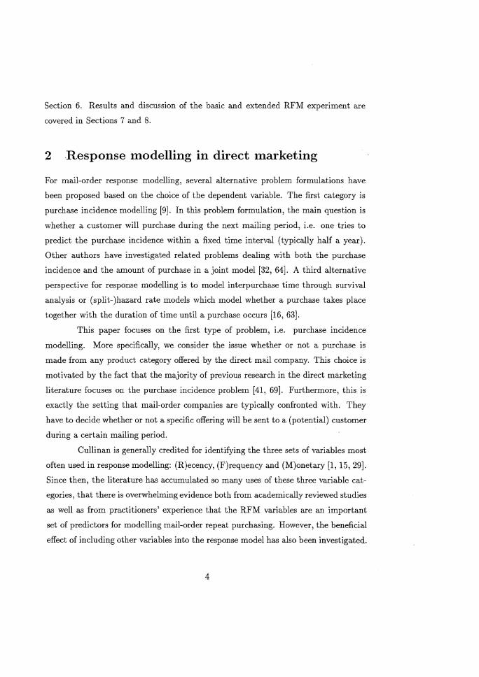
The substantive relevance of response modelling comes from the fact that

an increase in response of only one percentage point can result in substantial profit

increases, as the following real-life example of an actual mail-order company illus­

trates. Suppose that the mail-order company decides to mail to 75% of its current

mailing list of 5 million customers, i.e. 3,750,000 mailings are sent out. Suppose

that the overall response rate when mailing to all of their current customers is 10%

during a particular mailing period, i.e. if everyone would be mailed, 500,000 or­

ders would be placed. Suppose further that the average contribution per customer

amounts to 100 Euro, which is the typical real-life situation of a large mail-order com­

pany. Table 2 compares the economics of several alternative response models. When

no model is available, we can expect to obtain 75% of all potential responses (i.e.

0.75 x 500,000 = 375,000 responses) when 75% of 5 million people are mailed (i.e.,

3.75 million mailings are sent out). The ideal model (at the specific mailing depth)

is able to select the people from the mailing list in such a way that the 500, 000 po­

tential customers all receive a mailing, i.e. even though 25% of the mailing list is not

mailed, not a single order is lost. Suppose further that the current response model

used by the company, by mailing to 75% of their mailing list, allows to obtain 90% of

the responses, i.e. even though 1,250,000 people on the list do not receive a mailing,

only 10% of the 500,000 potential customers are excluded. This will result in 450, 000

orders, which represents a substantial improvement over the 'null model' situation.

If a better response model can be built, which achieves 91 % of the responses instead

of 90%, the contribution of this change will directly increase the contribution over

the null model from 7.50 million Euro to 8 million Euro, i.e. by 500,000 Euro (1%

of 10% of 5 million customers xl00 Euro average contribution).

Given a tendency of rising mailing costs and increasing competition, we can

easily see an increasing importance for response modelling [25]. Improving the target-

5

Reference Independent variable Dependent variable R F M Length of Other Socio- Binary Binary Binary

Relationship behavioural demographic and Amount and Timing

Berger and Magliozzi (1992) [2] X X X X X Bitran and Mondschein (1996)[5] X X X X

Bult and Wittink (1996)[11] X X X X Bult (1993) [9] X X X Bult (1993) [8] X X X X

Bult et al. (1997) [10] X X X X X X X Desarbo and Ramaswamy (1994)[18] X

Goniil and Shi(1998)[23] X X X I

Kaslow (1997)[28] X X X X X X X I

Levin and Zahavi (1998) [32] X X X X X X X Magliozzi and Berger (1993)[38] X X X X

Magliozzi (1989)[37] X X X X Rao and Steckel (1994)[47] X

0') Trasher (1991)[61] X X X X X Van den Poel (1999) [62] X X X X X X

Van der Scheer (1998) [64] X X X Zahavi and Levin (1997)[69] X X X X X

Table 1: Literature review of response modelling papers.

Type of Mailing No. of Customers No. of Mailings No. of Average Total Contribution Additional Contribution Model Depth (million) sent out (million) Responses Contribution (Euro) (million Euro) over 'No model' (million Euro)

Null Model 75.00 % 5.00 3.75 375,000 100.00 37.50 0.00

Ideal Model 75.00 % 5.00 3.75 500,000 100.00 50.00 12.50

90 % model 75.00 % 5.00 3.75 450,000 100.00 45.00 7.50

91 % model 75.00 % 5.00 3.75 455,000 100.00 45.50 8.00

Table 2: Economics resulting from performance differences among response models.

ing of the offers may indeed counter these two challenges by lowering non-response.

Moreover, from the perspective of the recipient of the (direct mail) messages, mail­

order companies do not want to overload consumers with catalogs. The importance

of response modelling to the mail-order industry is further illustrated by the fact that.

the issue of improving targeting was among the top three concerns with 73.5% of the

catalogers in the sample mentioned in [19].

In this study, we contribute to the literature by providing a thorough in­

vestigation into: (1) the suitability of Bayesian neural networks for repeat purchase

modelling; (2) the predictive performance of alternative operationalisations of RFM

variables and their relative importance; (3) the issue whether other (non-RFM) vari­

ables add predictive power to the traditional RFM variables.

3 Neural networks for pattern recognition

Neural networks (NNs) have shown to be very promising supervised learning tools

for modelling complex non-linear relationships [4, 50, 71]. NNs are designed to deal

with both regression and classification tasks. This, especially in situations where one

is confronted with a lack of domain knowledge. As universal approximators, they

can significantly improve the predictive accuracy of an inference model compared to

mappings that are linear in the input variables [26]. In what follows, the discussion

will be limited to the binary classification problematic. Typical application areas

include medical applications [39, 44, 53], business failure prediction [14, 30, 55, 70]

and customer credit scoring [17, 22, 45].

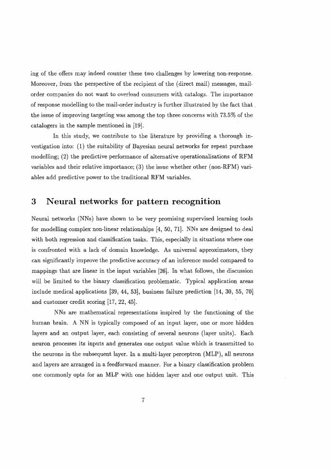
NNs are mathematical representations inspired by the functioning of the

human brain. A NN is typically composed of an input layer, one or more hidden

layers and an output layer, each consisting of several neurons (layer units). Each

neuron processes its inputs and generates one output value which is transmitted to

the neurons in the subsequent layer. In a multi-layer perceptron (MLP), all neurons

and layers are arranged in a feedforward manner. For a binary classification problem

one commonly opts for an MLP with one hidden layer and one output unit. This

7

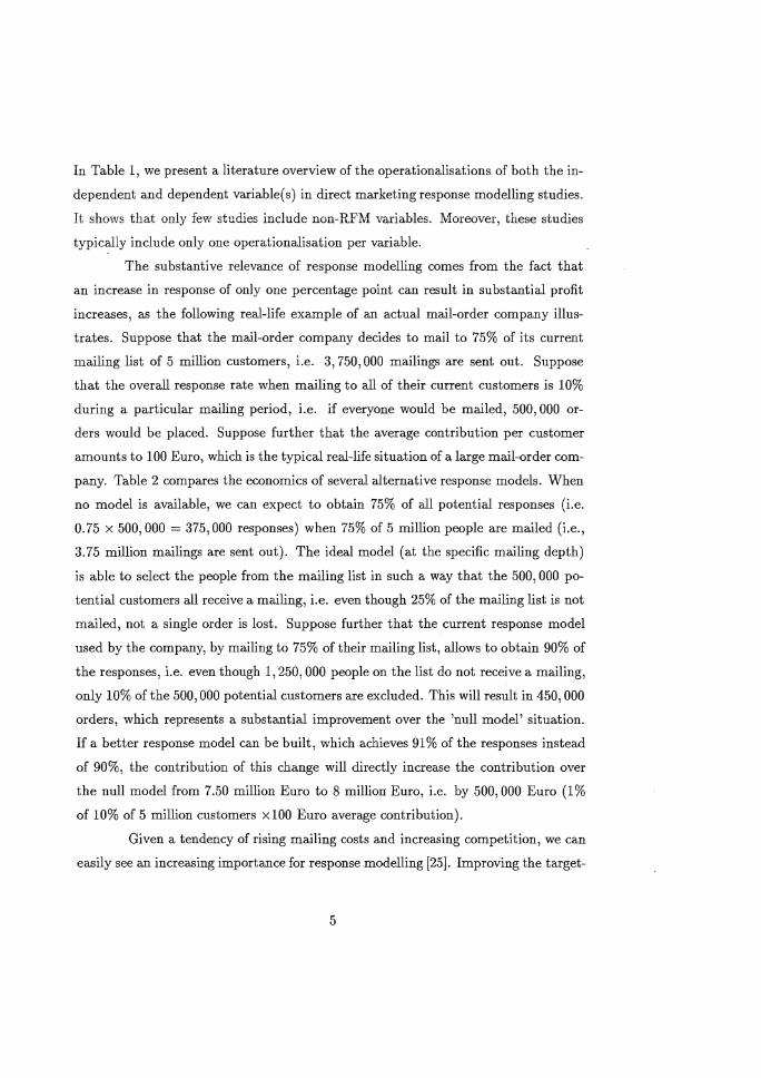
lnpuJl.ayer

Figure 1: A multi-layer perceptron with one hidden layer and one output unit.

neural network then performs the following non-linear function mapping

(1)

where x E IRn and y E IR is the MLP produced output. WI and W2 are weight vectors

of the hidden and output layer, respectively. The weight vectors WI and W2 together

make up the parameter vector w, which needs to be estimated (learned) during a

training process. II and 12 are termed transfer functions and essentially allow the

network to perform complex non-linear function mappings. An example of an MLP

with one hidden layer and one output unit is presented in Figure 1.

Given a training data set D = {x{m), tim) 1m = 1, ... , N}, where x{m) is an n­

dimensional input vector corresponding to a specific data instance m that is labelled

by a target variable t{m), the weight vector w of the NN is randomly initialised and

iteratively adjusted so as to minimise an objective function, typically the sum of

squared errors (SSE)

En = ! £: (t{m) _ y{m»)2. 2 m=I

(2)

The backpropagation algorithm originally proposed by Rumelhart et al. is probably

8

the best known example of the above mechanics [52]. It performs the optimisation

by using repeated evaluation of the gradient of ED and the chain rule of derivative

calculus. Due to the problems of slow convergence and relative inefficiency of this

algorithm, new and improved optimisation methods (e.g. Levenberg-Marquardt and _

Quasi-Newton) have been suggested to deal with the latter. For an overview, see [4].

For a binary classification problematic it is convenient to use the logistic

transfer function 1

J(z) = 1 + exp(-z) (3)

as transfer function in the output layer (J2), since its output is limited to a value

within the range [0,1]. This allows the output y(m) of a neural network to be inter­

preted as a conditional probability of the form p(t(m) = llx(m)) [4]. In that way, the

neural network naturally produces a score per data instance, which allows the data

instances to be ranked accordingly for scoring purposes (e.g. customer scoring). It

has to be noticed that for classification purposes the sum of squared error function

ED (see Eq.2) is no longer the most appropriate optimisation criterion because it was

derived from maximum likelihood on the assumption of Gaussian distributed target

data [4, 7, 56]. Since the target attribute is categorical in a classification context, this

assumption is no longer valid. A more suitable objective function is the cross-entropy

function which is based on the following rationale [4]. Suppose we have a binary

classification problem for which we construct a NN with a single output represent­

ing the posterior probability y(m) = p(t(m) = llx(m)). The likelihood of observing

t(m) E {O, I} given x(m) is then given by

(4)

The likelihood of observing the training data set is then modelled as

(5)

The cross-entropy error function G maximises this likelihood by minimising its neg-

9

ative logarithm

G = - L {t(m)ln(y(m)) + (1 - t(m))ln(1 _ y(m))}. (6) m

It can easily be verified that this error function reaches its minimum when y(m) = t(m)

for all m = 1, ... , N. Optimisation of G with respect to w may be carried out by using

the optimisation algorithms mentioned in [4].

For decision purposes, the posterior probability estimates produced by the

NN are used to classify the data instances into the appropriate (predefined) classes.

This is done by choosing a threshold value in the scoring interval [0,1]. The optimal

choice of this threshold value can be related to the probabilistic interpretation of the

network outputs as follows. Suppose we have two classes, class 1 (t(m) = 1) and class

o (t(m) = 0). As mentioned above, the output of the NN represents the estimated

probability that a particular data instance m belongs to class 1 given its input vector

x(m). The misclassification percentage is then minimised by assigning an instance

x(m) to the class c E {0,1} (i.e. tim) = c) having the largest posterior probability

estimate p(t(m) = clx(m)). This simply comes down to choosing a threshold value of

0.5. A data instance is assigned to class 1 if its output (posterior) probability exceeds

this threshold and to class 0 otherwise. Notice that this reasoning is contingent on a

situation in which equal misclassification costs are assigned to false positive and false

negative predictions.

The ultimate goal of NN training, and eventually of every inference mechan­

ism, is to produce a model which performs well on new, unseen test instances: If this

is the case, we say that the network generalises well. To do so, we basically have to

avoid the network from fitting the noise or idiosyncracies in the training data. This

is most often realised by monitoring the error on a separate validation set during

training of the network. When the error measure on the latter set starts to increase,

training is stopped, thus effectively preventing the network from fitting the noise in

the training data (early stopping). A superior alternative is to add a penalty term

10

(weight regulariser) to the objective function as follows [4, 58J

F(w) = G + aEw (7)

whereby, typically

(8)

with i running over all elements of the weight vector w. This method for improving

generalisation constrains the size of the network weights wand is referred to as

regularisation. When the weights are kept small, the network response will be smooth.

This decreases the tendency of the network to fit the noise in the training data.

The success of NNs with weight regularisation obviously depends strongly on

finding appropriate values for the weight vector wand the hyperparameter a. In the

next Section, we discuss the evidence framework of MacKay as our method of choice

for training the NN weight vector wand setting the hyperparameter a [33, 34, 35].

4 The evidence framework

Bayesian learning essentially works by adapting prior probability distributions into

posterior probability distributions guided by the training data [4, 33, 34, 35, 42J.

Relying on probability distributions stresses the importance of capturing the inherent

uncertainty while learning the true relationship from a finite data sample. In a

Bayesian context, all implicit assumptions, i.e. prior knowledge encoded in the form

of prior probability distributions, have to be made explicit and rules are provided

for reasoning consistently given those assumptions. More specifically, in a Bayesian

NN learning framework, the weights of the neural network are considered random

variables and are characterised by a joint probability distribution. In this Section, we

restrict our attention to the evidence framework for Bayesian learning as introduced

by MacKay in [33, 34, 35J. Other implementations of Bayesian learning have been

presented in e.g. [12,42, 68J.

Let p(wla, H) be the prior probability distribution over the weight vector w

11

given a neural network model H and the hyperparameter a. p(wla, H) expresses our

initial beliefs about the weights w before any data has arrived. This will typically be

a flat (uniform) distribution in the weight space when all weight values are a priori

equiprobable. When the data D are observed, the prior distribution of the parameter _

vector w is adjusted to a posterior distribution according to Bayes' theorem (level-1

inference). This gives

( ID H) = p(Dlw,H)p(wla,H) P w ,a, p(Dla,H)· (9)

In the above expression p(Dlw, H) is the likelihood function, which is the probability

of the data occurring given the weights w and the functional form of the neural

network H. The denominator of the expression in Eq.(9), i.e. p(Dla, H), is the

normalisation factor that guarantees that the right hand side of Eq.(9) integrates to

one over the weight space. The latter is often referred to as the evidence for a. Hence,

Eq.(9) can be restated as

. likelihood x prior posterIor = .d

eVI ence (10)

Obtaining good predictive models is dependent on the use of the right prior

distributions. MacKay uses Gaussian prior distribution functions in his operation­

alisation of Bayesian learning to approximate the posterior p(wID, a, H). In e.g.

[12, 68] other types of prior distributions have been used. When assuming a Gaussi­

an prior for the weights w with zero mean and variance equal to ~, the probability

distributions in the numerator of the right hand side of Eq.(9) can be written as

p(Dlw,H) = lIm (y(m»)t(m) (1 _ y(m»)I-t(m)

exp(-G) (11)

p(wla,H) = Z~(Oi)exp(-aEw)

with Zw (a) = (2;) ~ and I standing for the number of weight parameters. By substi-

12

tuting these probabilities into Eq.(9), we obtain

p(wID, a, H) = ~exp(-(G+aEw))

evidenct"

(12)

= z:(a)exp( -F(w)).

The most probable weights w MP can then be chosen so as to maximise the posterior

probability p(wID, a, H). This is equivalent to minimising the regularised objective

function F(w) = G + aEw , since ZM(a) is independent of the weights w. The

most probable weight values w MP (given the current setting of a) are thus found

by minimising the objective function F(w). Standard optimisation methods may be

used to perform this task [4]. This concludes the first level of Bayesian inference.

Notice how Eq.(9) assumes that the value for the hyperparameter a is known,

since the probability distributions were formulated as being contingent on the values

of a. The hyperparameter a may again be optimised by applying Bayes' theorem,

which is typical in an optimisation framework governed by Bayesian reasoning (level-2

inference). This yields

( ID H) = p(Dla, H)p(aIH) p a , p(DIH). (13)

Starting from Eq.(13) and assuming a uniform (non-informative) prior distribution

p( aIH), the most probable a, aMP, is obtained by maximising the likelihood function

p(Dla, H). Notice that this likelihood function performs the role of the normalising

constant in Eq.(9), where it was referred to as the evidence for a. Making" use of

Eq.(9) and making the Gaussian prior explicit, we can rewrite the normalisation

13

factor as p(Dla, H) p(Dlw,H)p(wla,H)

p(wID,a,H)

exp( -G) ~exp( -aEw)

Z~(,,)exp(-F(w))

ZM(a) exp(-G-aEw ) Zw(a) exp(-F(w))

ZM(a) Zw(a)"

(14)

Zw(a) is known from its definition in Eq.(ll). The only part we need to determine

in order to be able to optimise Eq.(14) is ZM(a). The latter may be estimated by

demanding that the right hand side of Eq.(12) integrates to one over the weight

space and approximating F(w) by a second order Taylor series expansion around

w MP . The hyperparameter aMP may then be found by setting the derivative of the

logarithm of Eq.(14) with respect to a to zero yielding

(15)

where '"Y = l - aTrace(HMP)-l is called the effective number of parameters in the

neural network. For more mathematical details see MacKay (33, 34, 35]. H MP stands

for the Hessian matrix of the objective function F(w) evaluated at w MP . The effective

number of parameters in a trained neural network is the number of well determined

weights indicating how many parameters of the NN are effectively used in reducing

the error function F(w). It can range from 0 to l. The a parameter is randomly

initialised and the network is then trained in the usual manner by using standard

optimisation algorithms [4], with the novelty that training is periodically halted for

the weight decay parameter a to be updated. The latter may be done at each epoch

of the NN training algorithm or after a fixed number of epochs. Notice that, since

no validation set is required, all data can be used for training purposes.

An aspect of Bayesian learning we have not mentioned yet is model selec­

tion (level-3 inference). It is possible to choose between network architectures in a

14

Bayesian way by using the evidence attributed to an architecture H referred to as

p(DIH) in [33, 34, 35]. Network models may then be ranked according to their evid-

ence. However, in [51] it was empirically shown tha~t for large data sets, the training

error is as good a measure for model selection as is the evidence. For further de-_

tails on Bayesian learning for neural networks we refer to [4, 33, 34, 35, 42]. In the

next Section, we present another aspect of the evidence framework that plays an im­

portant role in the setup of this paper: input ranking using the automatic relevance

determination method.

5 Input ranking using automatic relevance determ­

ination (ARD)

Selecting the best subset of a set of n input variables as predictors for a neural

network is a non-trivial problem. This follows from the fact that the optimal input

subset can only be obtained when the input space is exhaustively searched. When

n inputs are present, this would imply the need to evaluate 2n - 1 input subsets.

Unfortunately, as n grows, this very quickly becomes computationally infeasible [27].

For that reason, heuristic search procedures are often preferred. A multitude of

input selection methods have been proposed in the context of neural networks [40,

48, 49, 54]. These methods generally rely on the use of sensitivity heuristics, which

try to measure the impact of input changes on the output of the trained network.

Inputs may then be ranked (soft input selection) and/or pruned (hard input selection)

according to their sensitivity values. In this paper, we focus on input ranking as a

means to assess the relative importance of the various inputs for the direct marketing

case at hand. This is done by using the automatic relevance determination method

[36,43]. The ARD model is easily integrated within the evidence framework outlined

in the previous Section. It allows to perform soft input selection by ranking all inputs

according to their relative importance for the trained network.

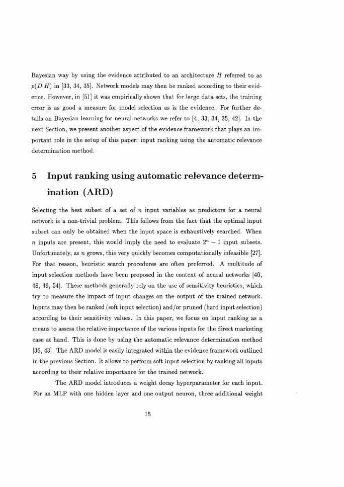
The ARD model introduces a weight decay hyperparameter for each input.

For an MLP with one hidden layer and one output neuron, three additional weight

15

decay constants are introduced: one associated with the connections from the input

bias to the hidden neurons, one associated with the connections from the hidden

neurons to the output neuron and one associated Vi lith the connection from the hid-

den bias neuron to the output neuron. This means that n + 3 weight classes, each.

associated with one weight decay parameter O!k, are considered when n inputs are

present. This setup is illustrated in Figure 2. All weights of weight class k are then

assumed to be distributed according to a Gaussian prior with mean 0 and variance

d = ,L (see Eq.(ll)). The evidence framework is thereupon applied to optimise all

n + 3 hyperparameters ak by finding their most probable values a~p.

The most probable weights w MP are found by minimising the altered object­

ive function

F(w) = G + I>kEW(k) (16) k

where EW(k) = ! I:i w;, with i running over all weights of weight class k. Analogous

to the results obtained in the previous Section, one obtains (level-2 inference)

(17)

"Yk is the number of well determined parameters for weight class k with "Yk = lk -

akTracek(HMP)-l. lk is the number of parameters (weights) in weight class k and

the trace is taken over those parameters only. All inputs may eventually be ranked

according to their optimised ak values. The most relevant inputs will have the lowest

O!k values, since ak is inversely proportional to the variance around 0 of the corres­

ponding Gaussian prior.

One of the main advantages of ARD is that it allows to include a large

number of potentially relevant input variables in the model without damaging effects

[43J. Furthermore, it is integrated into the optimisation mechanism and completely

rests upon the inspection of the optimised ak parameters. Illustrations of ARD for

input ranking can be found in [6, 13, 36, 42, 43, 67J.

16

InputLayer

Figure 2: Overview of the Ok hyperparameters introduced by the ARD method.

6 Design of the study

6.1 Data set

From a major European mail-order company, we obtained data on past purchase

behaviour at the order-line level, i.e. we know when a customer purchased what

quantity of a particular product at what price as part of what order. This allowed

us, in close cooperation with domain experts and guided by the extensive literature

(see Section 2), to derive all the necessary purchase behaviour variables for.a total

sample size of 100,000 customers. For each customer, these variables were measured

in the period between July pt 1993 and June 30th 1997. The goal is to predict

whether an existing customer will repurchase in the observation period between July

pt 1997 and December 31"t 1997 using the information provided by the purchase

behaviour variables. This problem boils down to a binary classification problem:

Will a customer (data instance m) repurchase (t(m) = 1) or not (t(m) = 0)7 Again

notice that the focus is on customer retention and not on customer acquisition. Of

the 100,000 customers, 55.18% actually repurchased during the observation period.

17

6.2 Experimental setup

The experiment consists of two sub-experiments. In Section 7, we start by concen­

trating on RFM variables only. Using these variables, we compare the performance

of NNs trained using the evidence framework with that of three benchmark statistic- -

al classification techniques i.c. logistic regression, linear and quadratic discriminant

analysis. We then discuss the relevance of the RFM variables using the ARD method

presented in Section 5. In an attempt to further enrich the RFM response model, the

same experiment is repeated with the input of other, potentially interesting customer

profiling predictors which were handpicked by domain experts.

All performance assessments are computed on 10 bootstrap resamples gen­

erated from the original data set. Each bootstrap consists of 100,000 instances which

are divided into a training set (50,000 instances) and a test set (50,000 instances). The

former is used to train the classifier and the latter is used to estimate its generalisa­

tion behaviour. As a form of preprocessing, the inputs are statistically normalised to

zero mean and unit variance by subtracting their mean and dividing by the standard

deviation [4]. This is needed in order to be able to compare the relative importance

of the various inputs by means of the ARD hyperparameters.

All neural network classifiers have one hidden layer with hyperbolic tangent

transfer functions. A logistic transfer function is used in the output layer. The

architecture of the MLP is determined by varying the number-of hidden units between

2 and 14 in steps of 2. The hidden units have connections to all input units and also

have a bias input. The single output is connected to all hidden units and agai? has a

bias input. The number of epochs is set to 1,000. The hyperparameter a is initialised

to 0.2. All neural networks are trained with the Quasi-Newton method to minimise a

regularised cross-entropy error function. The hyperparameter a is updated every 100

epochs. All trained classifiers are evaluated by looking at their performance assessed

on the independent test sets of all 10 bootstraps. All neural network analyses were

done using the Netlab toolbox for Matlab implemented by Bishop and Nabney [4]. In

the following Subsection we provide an overview of the performance measures which

were used in this paper.

18

6.3 Performance criteria for classification

The percentage correctly classified (PCC) cases, also known as the overall classifica­

tion accuracy, is undoubtedly the most commonly used measure of the performance

of a dassifier. It simply measures the proportion of correctly classified cases on a·

sample of data D. Formally, it can be described as

PCC = ~ ~ o(y(m) t(m») N L.." 0,1 , m=l

(18)

where y~~) is the predicted class for instance m, t(m) is its true class label and 0(.,.)

stands for the Kronecker delta function which equals 1 if both arguments are equal,

o otherwise.

In a number of cases, the overall classification accuracy may not be the most

appropriate performance criterion. It tacitly assumes equal misclassification costs for

false positive and false negative predictions. This assumption is problematic, since

for most real-world problems (e.g. fraud detection, customer credit scoring) one type

of classification error may be much more expensive than the other. Another implicit

assumption of the use of pee as an evaluation metric is that the class distribution

(class priors) among examples is presumed constant over time and relatively balanced

[46). For example, when confronted with a situation characterised by a very skewed

class distribution in which faulty predictions for the underrepresented class are very

costly, a model evaluated on pee alone may always predict the most common class

and, in terms of pee, provide a relatively high performance. Thus, using pce alone

often proves to be inadequate, since class distributions and misclassification costs are

rarely uniform. However, taking into account class distributions and misclassification

costs proves to be quite hard, since in practice they can rarely be specified precisely

and are often subject to change [21). In spite of the above, comparisons based on

classification accuracy often remain useful because they are indicative of a broader

notion of good performance [46].

Descriptive statistics such as the false positives, false negatives, sensitivity

and specificity can provide more meaningful results. Class-wise decomposition of the

19

classification of cases yields a confusion matrix as specified in Table 3. The following

.H.c"ua!

Predicted + -

+ True Positive (TP) False Positive (FP)

- False Negative (FN) True Negative (TN)

Table 3: The confusion matrix for binary classification.

performance metrics can readily be distilled from Table 3

.. . TP sensItivIty = TP + FN (19)

'fi . TN speer CIty = FP + TN (20)

The sensitivity (specificity) measures the proportion of positive (negative) examples

which are predicted to be positive (negative). Using the notation of Table 3, we may

now formulate the overall accuracy as follows

TP+TN PCC = TP + FP + TN + FN (21)

Note that sensitivity, specificity and PCC vary together as the threshold on a classi­

fier's continuous output is varied between its extremes within the interval [0,1]. The

receiver operating characteristic curve (ROC) is a 2-dimensional graphical illustration

of the sensitivity ('true alarms') on the Y-axis versus (I-specificity) (,false alarms')

on the X-axis for various values of the classification threshold. It basically illustrates

the behaviour of a classifier without regard to class distribution or error cost, so it

effectively decouples classification performance from these factors [20, 59, 60].

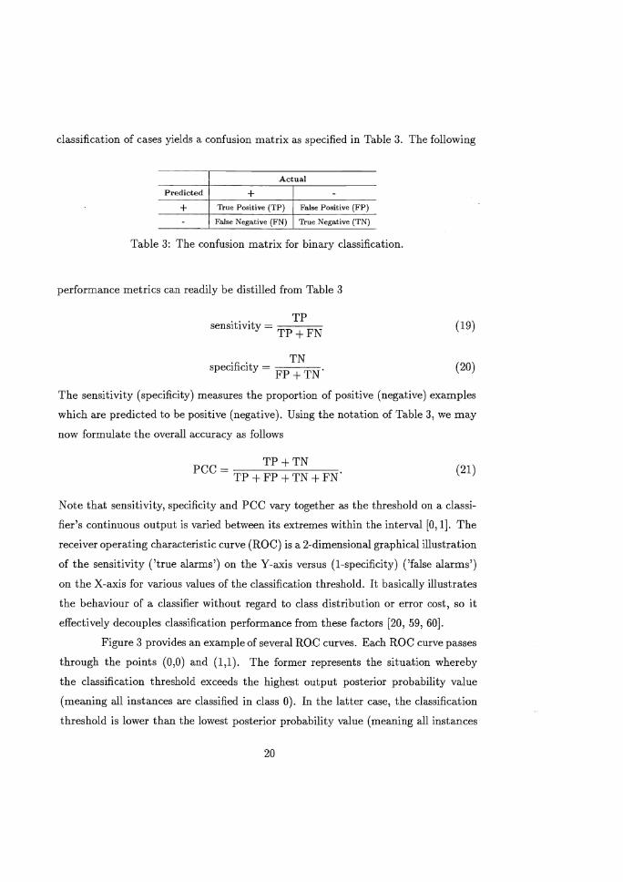
Figure 3 provides an example of several ROC curves. Each ROC curve passes

through the points (0,0) and (1,1). The former represents the situation whereby

the classification threshold exceeds the highest output posterior probability value

(meaning all instances are classified in class 0). In the latter case, the classification

threshold is lower than the lowest posterior probability value (meaning all instances

20

are classified in class 1). A straight line through (0,0) and (1,1) represents a classifier

with poor discriminative power, since the sensitivity always equals (I-specificity) for

all possible values of the classification threshold (curve A). It is to be considered

as a benchmark for the predictive accuracy of other classifiers. The more the ROC _

curve approaches the (0,1) point, the better the classifier will discriminate (e.g. curve

D dominates curves A, B and C). ROC curves of different classifiers may however

intersect making a performance comparison less obvious (e.g. curves B and C). To

overcome this problem, one often calculates the area under the receiver operating

characteristic curve (AUROC). The AUROC provides a simple figure-of-merit for the

performance of the constructed classifier. An intuitive interpretation of the AUROC

is that it provides an estimate of the probability that a randomly chosen instance

of class 1 is correctly rated (or ranked) higher than a randomly selected instance of

class a [24].

Figure 3: The receiver operating characteristic curve (ROC).

In what follows, we consistently multiply AUROC values by a factor of 100 to

give a number that is similar to PCC, with 50 indicating random and 100 indicating

perfect classification.

21

7 Basic RFM experiment

7.1 Predictors used in the basic RFM experiment

We used two time horizons for all RFM variables. The Hist horizon refers to the fact .

that the variable is measured between the period July pt 1993 until June 30th 1997.

The Year horizon refers to the fact that the variable is measured over the last year.

Including both time horizons allows us to check the argumentation that more recent

data is much more relevant than historical data. All RFM variables are modelled

both with and without the occurrence of returned merchandise, indicated by Rand

N in the variable name, respectively. The former is operationalised by including the

counts of returned merchandise in the variable values, whereas in the latter case these

counts are omitted. Taking into account both time horizons (Year versus Hist) and

inclusion versus exclusion of returned items (R versus N), we arrive at a 2 x 2 design

in which each RFM variable is operationalised in 4 ways.

For the Recency variable, many operationalisations have already been sug­

gested. In this paper, we define the Recency variable as the number of days since the

last purchase within a specific time window (Hist versus Year) and in- or excluding

returned merchandise (R versus N) [1]. Recency has been found to be inversely re­

lated to the probability of the next purchase, i.e. the longer the time delay since the

last purchase the lower the probability of a next purchase within the specific period

[15].

In the context of direct mail, it has generally been observed that multi-buyers

(buyers who already purchased several times) are more likely to repurchase than

buyers who only purchased once [1, 57]. Although no detailed results are reported

because of the proprietary nature of most studies, the Frequency variable is generally

considered to be the most important of the RFM variables [41]. Bauer suggests to

operationalise the Frequency variable as the number of purchases divided by the time

on the customer list since the first purchase [1]. We choose to operationalise the

Frequency variable as the number of purchases made in a certain time period (Hist

versus Year) while in- or excluding returned merchandise (R versus N).

22

In the direct marketing literature, the general convention is that the more

money a person has spent with a company, the higher his/her likelihood of purchasing

the next offering [31]. l'Jash suggests to operationalise 1110netary value as the highest

transaction sale or as the average order size [41]. Levin and Zahavi propose to use the _

average amount of money per purchase [31]. We model the Monetary variable as the

total accumulated monetary amount of spending by a customer during a certain time

period (Hist versus Year) while in- or excluding returned merchandise (R versus N).

Table 4 gives an overview of the different operationalisations of the RFM variables.

Recency Frequency Monetary RecHistN FrHistN MonHistN RecHistR FrHistR MonHistR RecYearN FrYearN MonYearN RecYearR FrYearR MonYearR

Table 4: Operationalisations of RFM variables used in the basic RFM experiment.

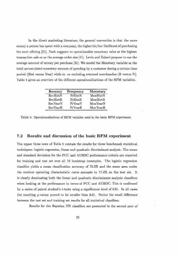
7.2 Results and discussion of the basic RFM experiment

The upper three rows of Table 5 contain the results for three benchmark statistical

techniques: logistic regression, linear and quadratic discriminant analysis. The mean

and standard deviation for the pee and AUROe performance criteria are reported

for training and test set over all 10 bootstrap resamples. The logistic regression

classifier yields a mean classification accuracy of 70.3% and the mean area under

the receiver operating characteristic curve amounts to 77.4% on the test set. It

is clearly dominating both the linear and quadratic discriminant analysis classifiers

when looking at the performance in terms of pee and AUROe. This is confirmed

by a series of paired student's t-tests using a significance level of 0.01. In all cases

the resulting p-values proved to be smaller than 0.01. Notice the small difference

between the test set and training set results for all statistical classifiers.

Results for the Bayesian NN classifiers are presented in the second part of

23

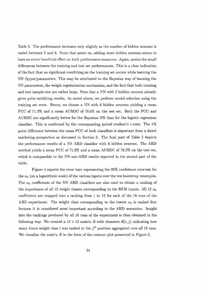
Table 5. The performance increases only slightly as the number of hidden neurons is

varied between 2 and 6. From that point on, adding more hidden neurons seems to

have no extra beneficial effect on both performance measures. Again, notice the small

differences between the training and test set performances. This is a clear indication.

of the fact that no significant overfitting on the training set occurs while learning the

NN (hyper )parameters. This may be attributed to the Bayesian way of learning the

NN parameters, the weight regularisation mechanism, and the fact that both training

and test sample size are rather large. Note that a NN with 2 hidden neurons already

gives quite satisfying results. As noted above, we perform model selection using the

training set error. Hence, we choose a NN with 6 hidden neurons yielding a mean

pee of 71.3% and a mean AUROe of 78.6% on the test set. Both the pee and

AUROe are significantly better for the Bayesian NN than for the logistic regression

classifier. This is confirmed by the corresponding paired student's t-tests. The 1%

point difference between the mean pee of both classifiers is important from a direct

marketing perspective as discussed in Section 2. The final part of Table 5 depicts

the performance results of a NN ARD classifier with 6 hidden neurons. The ARD

method yields a mean pee of 71.2% and a mean AUROe of 78.5% on the test set,

which is comparable to the NN non-ARD results reported in the second part of the

table.

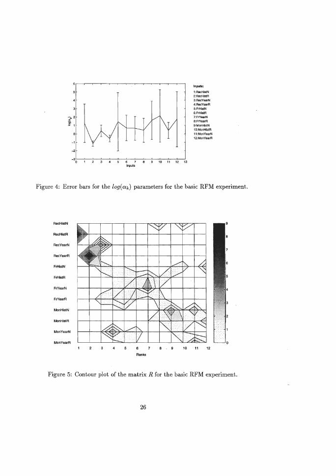
Figure 4 reports the error bars representing the 95% confidence intervals for

the Cik (on a logarithmic scale) ofthe various inputs over the ten bootstrap resamples.

The Cik coefficients of the NN ARD classifiers are also used to obtain a ranking of

the importance of all 12 weight classes corresponding to the RFM inputs. A1112 Cik

coefficients are mapped into a ranking from 1 to 12 for each of the 1D runs of the

ARD experiment. The weight class corresponding to the lowest Cik is ranked first

because it is considered most important according to the ARD semantics. Insight

into the rankings produced by aUlD runs of the experiment is then obtained in the

following way. We created a 12 x 12 matrix R with elements R(i,j) indicating how

many times weight class i was ranked at the /h position aggregated over all1D runs.

We visualise the matrix R in the fOfm of the contour plot presented in Figure 5.

24

There is broad agreement between both plots concerning the relative import­

ance of the inputs. The dark zone in the contour plot at the intersection of rank 1

and the RecHistR variable clearly indicates its importance. This variable was 10

times ranked first. The RecYearR and RecYearN variables seem to be very useful as

well. Note that the RecYearR variable was always ranked second over all 10 runs.

These findings are confirmed by the relatively low mean log(ak) values and narrow

confidence intervals for the RecHistR, RecYearR and RecYearN variables as depicted

in Figure 4. The rankings of the variables belonging to the Frequency category are

concentrated in the zone covering ranks 4 to 8. This suggests that these variables are

of medium importance to the NN prediction. The ranking of the Mon YearN variable

is concentrated around rank 4. The other Monetary variables are ranked between

ranks 8 and 12. Figure 4 also indicates that the Mon YearN variable is the most

important among the set of Monetary predictors. Notice that neither plot clearly

indicates the irrelevance of predictors included in the study. Therefore, we conclude

that a combined use of predictors of all three categories is desirable for response

modelling. Moreover, it can be stated that the way a variable is operationalised has

a substantial impact on its predictive performance.

pee AURoe

Train Test Train Test logistic regression 70.3 ± 0.1 70.3 ± 0.2 77.5 ± 0.1 77.4 ± 0.2 linear discriminant analysis 68.9 ± 0.1 68.9 ± 0.2 76.0 ± 0.1 75.9 ± 0.2 quadratic discriminant analysis 63.6 ± 0.4 63.2 ± 0.4 74.4 ± 0.2 74.3 ± 0.2 NN 2 hidden neurons 71.2 ± 0.1 71.2 ± 0.1 78.5 ± 0.1 78.4± 0.2 NN 4 hidden neurons 71.3 ± 0.2 71.2 ± 0.1 78.8 ± 0.2 78.5 ± 0.2 NN 6 hidden neurons 71.4 ± 0.2 71.3 ± 0.2 78.9 ± 0.2 78.6 ± 0.2 NN 8 hidden neurons 71.4 ± 0.2 71.3 ± 0.2 78.9 ± 0.2 78.6 ± 0.2 NN 10 hidden neurons 71.4 ± 0.2 71.3 ± 0.1 78.9 ± 0.2 78.6 ± 0.2 NN 12 hidden neurons 71.4 ± 0.2 71.3 ± 0.1 78.9 ± 0.2 78.6 ± 0.2 NN 14 hidden neurons 71.4 ± 0.2 71.3 ± 0.1 78.9 ± 0.2 78.6 ± 0.2 NN ARD 6 hidden neurons 71.4 ± 0.2 71.2 ± 0.1 78.7 ± 0.2 78.5 ± 0.2

Table 5: Performance assessment of all classifiers for the basic RFM experiment.

25

-1

-2

Inputs

Inputs:

1:RecHistN 2:RecHIsl:R 3:RecYearN 4:RecYearR 5:FrHlstN 6:FrHlstR 7:FrYearN 8:FrYearR 9:MonHlstN 10:MonHlstR 11 :MonYearN 12:MonYearR

Figure 4: Error bars for the loge (tk) parameters for the basic RFM experiment.

RecHistN

RecHistR

RecYearN

RecYearR

FrHistN

FrHislR

FrYearN

FrYearR

MonHistN

MonHistR

MonYearN

MonYearR

4 5 6 7 8 . 9 10 11 12

Ranks

Figure 5: Contour plot of the matrix R for the basic RFM experiment.

26

8 Extended RFM experiment

8.1 Predictors used in the extended RFM experiment

Apart. from the RFM variables discussed in Subsection 7.1, we now include 10 other·

customer profiling features (referred to as 'Other' in Table 6) [63].

The type and frequency of contact which customers have with the mail-order

company may yield important information about their future purchasing behaviour.

The Genlnfo and GenCust are binary customer/company interaction variables indic­

ating whether the customer asked for general information respectively filed general

complaints. Since customer (dis ) satisfaction may not only be revealed by general

complaints but also by returning items, we included two extra variables. The Ret­

Merch variable is a binary variable indicating whether the customer has ever returned

an item that was previously ordered from the mail-order company. The RetPerc vari­

able measures the total monetary amount of returned orders divided by the total

amount of spending. The N days variable models the length of the customer rela­

tionship in days. It is commonly believed that consumers/households with a longer

relationship with the company have a higher probability of repurchase than house­

holds with shorter relationships. IncrHist and IncrYear are operationalisations of a

behavioural loyalty measure. We propose to perform a median split of the length of

the relationship (time since the household became a customer). This enables us to

compare the number of purchases (i.e. frequency) between the first and last half of

the time window. The following formula is used

purchases second half-purchases first half purchases first half

(22)

If the above measure is positive, this may give us an indication of increasing loyalty

by that customer to the (mail-order) company, and ipso facto satisfaction with the

current level of service. Remember that the suffix Hist reflects that the whole purchase

history is used, whereas in the case of the suffix Year, only transactions from the last

year are included. The mail-order company has internal records whether a customer

uses the credit facilities. This may function as an indicator of the extent to which the

27

customer values the financial convenience of mail-order buying. Therefore, we also

include the binary Credit variable. The ProdclaT respectively ProdclaM variables

represent the total (T) respectively mean (~.,1) forvv"ard=looking '\rveighted productindex.

The weighting procedure represents the 'forward-looking' nature of a product category _

purchase, derived from another sample of data.

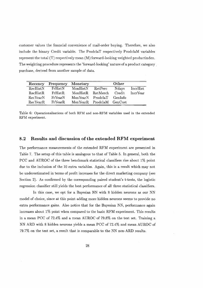
Recency Frequency Monetary Other RecHistN FrHistN MonHistN RetPerc Ndays IncrHist RecHistR FrHistR MonHistR RetMerch Credit IncrYear RecYearN FrYearN MonYearN ProdclaT GenInfo RecYearR FrYearR MonYearR ProdclaM GenCust

Table 6: Operationalisations of both RFM and non-RFM variables used in the extended RFM experiment.

8.2 Results and discussion of the extended RFM experiment

The performance measurements of the extended RFM experiment are presented in

Table 7. The setup of this table is analogous to that of Table 5. In general, both the

PCC and A UROC of the three benchmark statistical classifiers rise about 1 % point

due to the inclusion of the 10 extra variables. Again, this is a result which may not

be underestimated in terms of profit increases for the direct marketing company (see

Section 2). As confirmed by the corresponding paired student's t-tests, the logistic

regression classifier still yields the best performance of all three statistical cla~sifiers.

In this case, we opt for a Bayesian NN with 8 hidden neurons as our NN

model of choice, since at this point adding more hidden neurons seems to provide no

extra performance gains. Also notice that for the Bayesian NN, performance again

increases about 1% point when compared to the basic RFM experiment. This results

in a mean pce of 72.4% and a mean AUROC of 79.8% on the test set. Training a

NN ARD with 8 hidden neurons yields a mean pee of 72.4% and mean AUROe of

79.7% on the test set, a result that is comparable to the NN non-ARD results.

28

Again, Figure 6 presents the 95% confidence intervals for the Cik values on a

logarithmic scale. The matrix R associated with the weight class rankings is depicted

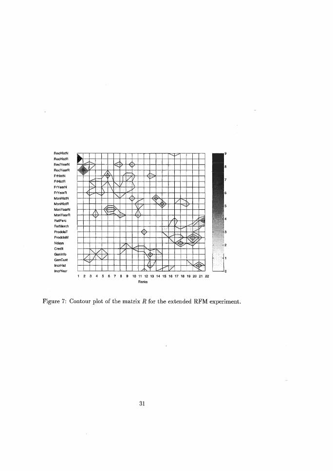
in the contour plot given by Figure 7. Among the RFM variables, the sarile relevance

patterns are present as for the basic RFM experiment, thus essentially confirming _

the latter. The rankings of the RetPerc, Ret Merch , ProdclaT, ProdclaM, Ndays,

IncrHist and IncrYear variables are concentrated in the region of lesser importance

in the contour plot. When looking at both plots, it can be observed that the Credit,

Genlnfo and GenCust variables are definitely more relevant to the trained networks.

The 1% point performance rise may thus be especially attributed to the inclusion of

these three variables in the extended RFM response model.

When comparing the results of this study to those on similar data sets from

the same anonymous company, reported in [62, 65, 66], we observe that the insight

gained using Bayesian neural network methods generally confirms previous findings.

Most noticeably they also highlight: (1) the importance of a combined use of all

three RFM predictor categories in predicting mail-order repeat purchase behaviour;

(2) the performance gains by including non-RFM variables into the response model.

However, there is some disagreement considering the relative importance of some of

the RFM and non-RFM variables. These differences may be due to: (1) different

data sets from different countries, resulting in a.o. diverging class proportions (i.e.,

38% buyers in [65, 66] compared to 55% buyers in this study); (2) inclusion of other

predictors or alternative transformations (e.g. logarithmic transformation to reduce

the skewness in [65, 66]); (3) the use of other classification techniques (e.g. support

vector machines in [66]) and input selection heuristics (e.g. hard sensitivity based

pruning in [65, 66]).

9 Conclusion

In this paper, we focus on purchase incidence modelling for a major European dir­

ect mail company. The case boils down to a binary classification problem: Will

the customer repurchase or not? Response models based on statistical and neur-

29

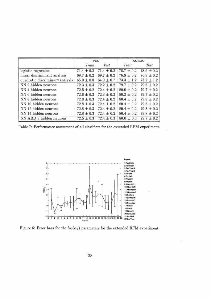
PCC AURoe

Train Test Train Test

logistic regression 71.4 ± 0.2 71.4 ± 0.2 78.7 ± 0.2 78.6 ± 0.2 linear discriminant analysis 69.7 ± 0.2 69.7 ± 0.2 76.9 ± 0.2 76.8 ± 0.2 quadratic discriminant analysis 65.0 ± 0.8 64.9 ± 0.7 73.3 ± 1.2 73.2 ± 1.2 NN 2 hidden neurons 72.3 ± 0.3 72.2 ± 0.2 79.7 ± 0.2 79.5 ± 0.2 NN 4 hidden neurons 72.5 ± 0.2 72.4 ± 0.2 80.0 ± 0.2 79.7 ± 0.2 NN 6 hidden neurons 72.6 ± 0.3 72.3 ± 0.2 80.2 ± 0.2 79.7 ± 0.2 NN 8 hidden neurons 72.8 ± 0.3 72.4 ± 0.2 80.4 ± 0.2 79.8 ± 0.2 NN 10 hidden neurons 72.8 ± 0.3 72.4 ± 0.2 80.4 ± 0.2 79.8 ± 0.2 NN 12 hidden neurons 72.8 ± 0.3 72.4 ± 0.2 80.4 ± 0.2 79.8 ± 0.2 NN 14 hidden neurons 72.8 ± 0.3 72.4 ± 0.2 80.4 ± 0.2 79.8 ± 0.2 NN ARD 8 hidden neurons 72.5 ± 0.3 72.4 ± 0.3 80.0 ± 0.3 79.7 ± 0.2

Table 7: Performance assessment of all classifiers for the extended RFM experiment.

-1

Inputs:

1:RacHls1N 2:RecHistR 3:RecYearN 4:RecYearR 5:FrHistN 6:FrHlstR 7:FrYearN 8:FrYearR 9:MonHlsIN 10:MonHlstR 11 :MonYearN 12:MonYesrR 13:RetPerc 14:ReIMerch 15:ProddaT 16:ProdclaM 17:Ndays 18:Cred/l 19:Genlnfo 2O:GenCust

-2 21 :lncrHlst o 1 2 3 4 5 6 7 8 9 10 :~~ 13 14 15 18 17 t8 19 20 21 22 23 22:lncrYear

Figure 6: Error bars for the log(ak) parameters for the extended RFM experiment.

30

RecHistN

RecHistR

RecYearN

RecYearR

FrHistN

FrHistR

FrYearN

FrYearR

MonHistN

MonHistR

MonYearN

MonYearR

RetPerc

RetMerch

ProdclaT

ProdclaM

Ndays

Credit

Genlnfo

GenCust

IncrHist

IncrYear

.... "" ./t--- ./

~ ~, V ~ ~ h~ r

./r-' IV I" vtm , V

IV ....., :::: / V -....

1\ '\':;:: I I

V b;;ij I :/< 1':'1'

"-V .'.

" .. ""-.

" ~ '\, A "',(fYX / " r-, "'V

" / I'\, / h ." 1/ I'\, 1/ i,\ '- I ) i',.. h:::-'

A / ,~

1 2 3 4 5 6 7 8 9 10 11 12 13 14 15 16 17 18 19 20 21 22

Ranks

Figure 7: Contour plot of the matrix R for the extended RFM experiment.

31

al network techniques are developed and contrasted. The latter are trained using

Bayesian neural network learning, a method that is fairly robust with respect to the

problems of overfitting and (hyper )parameter choice, problems that are typically en­

countered when implementing neural networks. The evidence framework of MacKay _

is used as an example implementation of Bayesian learning. The automatic relev­

ance determination (ARD) method is an additional feature of this framework that

allows to assess the relative importance of the inputs. The basic response models use

operationalisations of the traditionally discussed Recency, Frequency and Monetary

(RFM) predictor categories. In a second experiment, the RFM response framework

is enriched by the inclusion of other (non-RFM) customer profiling predictors. In

this study, we contribute to the literature by providing a thorough investigation into:

(1) the suitability of Bayesian neural networks for repeat purchase modelling; (2) the

predictive performance of alternative operationalisations of RFM variables and their

relative importance; (3) the issue whether other (non-RFM) variables add predictive

power to the traditional RFM variables. By means of experimental evaluation, it

is illustrated that, from a performance perspective, Bayesian neural networks offer

an interesting and viable alternative for purchase incidence modelling. Performance

of the trained classifiers is measured using the percentage correctly classified (PCC)

and the area under the receiver operating characteristic curve (AUROC). TheARD

results advocate a combined use of all three RFM predictor categories for response

modelling. Finally, as illustrated by a second experiment, the inclusion of non-RFM

variables allows to further augment the predictive power of the constructed classifi­

ers. The ARD results mainly attribute this rise to the inclusion of customer/company

interaction variables and to a variable measuring whether a customer uses the credit

facilities of the direct mail company.

Acknowledgements

This work was partly carried out at the Leuven Institute for Research on Information

Systems (LIRIS) of the Dept. of Applied Economic Sciences of the K.U.Leuven in

32

the framework of the KBC Insurance Research Chair, set up in September 1997 as a

pioneering cooperation between LIRIS and KBC Insurance. We thank prof. J.A.K.

Suykens (K.U.Leuven) for his comments and suggestions. V-Ie are also grateful to

prof. Marnik Dekimpe (K.U.Leuven) and prof. Joseph Leunis (K.U.Leuven) for their _

numerous useful comments on earlier versions of parts of this document.

References

[1] A. Bauer. A direct mail customer purchase model. Journal of Direct Marketing,

2(3):16-24, 1988.

[2] P. Berger and T. Magliozzi. The effect of sample size and proportion of buyers

in the sample on the performance of list segmentation equations generated by

regression analysis. Journal of Direct Marketing, 6(1):13-22, 1992.

[3] M.J.A. Berry and G. Linoff. Mastering Data Mining. John Wiley & Sons, Inc.,

Chicago, 2000.

[4] C.M. Bishop. Neural networks for pattern recognition. Oxford University Press,

1995.

[5] G.R. Bitran and S.V. Mondschein. Mailing decisions in the catalog sales industry.

Management Science, 42(9):1364-1381, 1996.

[6] B.V. Bonnlander. Nonparametric Selection of Input Variables for Connectionist

Learning. PhD thesis, University of Colorado, Department of Computer Science,

1996.

[7] J .S. Bridle. Neuro-computing: algorithms, architectures and applications, chapter

Probabilistic interpretation of feedforward classification network output, with

relationships to statistical pattern recognition. Springer-Verlag, 1989.

[8] J.R. Bult. Semiparametric versus parametric classification models: an applica­

tion to direct marketing. Journal of Marketing Research, 30:380-390, 1993.

33

[9] J.R. Bult. Target selection for direct marketing. PhD thesis, Groningen Uni­

versity, 1993.

[10] J.R. Bult, H. Van der Scheer, and T. \Nansbeek. Interaction between target and

mailing characteristics in direct marketing, with an application to health care·

fund raising. The International Journal of Research in Marketing, 14:301-308,

1997.

[11] J.R. Bult and D.R. Wittink. Estimating and validating asymmetric heterogen­

eous loss functions applied to health care fund raising. The International Journal

of Research in Marketing, 13:215-226, 1996.

[12] W.L. Buntine and A.S. Weigend. Bayesian back-propagation. Complex Systems,

5:603-643, 1991.

[13] F.R. Burden, M.G. Ford, D.C. Whitley, and D.A. Winkler. The use of automatic

relevance determination in qsar studies using bayesian neural networks. Journal

of Chemical Information and Computer Sciences, 40:1423-1430, 2000.

[14] L.K. Chang, 1. Han, and Y. Kwon. Hybrid neural network models for bankruptcy

predictions. Decision Support Systems, 18(1):63-72, 1996.

[15] G.J. Cullinan. Picking them by their batting averages' recency-frequency-

monetary method of controlling circulation. Manual release 2103. Direct

Mail/Marketing Association. N.Y., 1977.

[16] M.G. Dekimpe and Z. Degraeve. The attrition of volunteers. European Journal

of Operational Research, 98:37-51, 1997.

[17] V.S. Desai, J.N. Crook, and G.A. Overstreet Jr. A comparison of neural networks

and linear scoring models in the credit union environment. European Journal of

Operational Research, 95(1):24-37, 1996.

[18] W.S. Desarbo and V. Ramaswamy. Crisp: customer response-based iterative

segmentation procedures for response modeling in direct marketing. Technical

Working Paper 94-102, Marketing Science Institute, 1994.

34

[19] DMA(1998). Statistical Fact Book 1998. Direct Marketing Association, New

York,NY, 20th edition, 1998.

[20] J.P. Egan. Signal Detection Theory and ROC analysis. Series in Cognition and

Perception. Academic Press, New York, 1975.

[21] T. Fawcett and F. Provost. Adaptive fraud detection. Data Mining and Know­

ledge Discovery, 1-3:291-316, 1997.

[22] L.W. Glorfeld and B.C. Hardgrave. An improved method for developing neural

networks: the case of evaluating commercial loan creditworthiness. Computers

and Operations Research, 23(10):933-944, 1996.

[23] F. Goniil and M.Z. Shi. Optimal mailing of catalogs: a new methodology us­

ing estimable structural dynamic programming models. Management Science,

44(9):1249-1262, 1998.

[24] J.A. Hanley and B.J. McNeil. The meaning and use of the area under a receiver

operating characteristic (roc) curve. Radiology, 148:839-843, 1983.

[25] B. Hauser. The Direct Marketing Handbook, chapter List segmentation, pages

233-247. 1992.

[26] K. Hornik, M. Stinchcombe, and H. White. Multilayer feedforward networks are

universal approximators. Neural Networks, 2(5):359-366, 1989.

[27] G. John, R. Kohavi, and K. Pfleger. Irrelevant features and the subset selection

problem. In H. Hirsh and W. Cohen, editors, Machine Learning: proceedings

of the Eleventh International Conference, pages 121-129, San Francisco, 1994.

Morgan Kaufmann.

[28] G.A. Kaslow. A microeconomic analysis of consumer response to direct marketing

and mail order. PhD thesis, California Institute of Technology, 1997.

[29] R.D. Kestnbaum. The Direct Marketing Handbook, chapter Quantitative Data­

base Methods, pages 588-597. 1992.

35

[30] R.C. Lacher, P.K. Coats, C. Sharma Shanker, and L.F. Fant. A neural network

for classifying the financial health of a firm. European Journal of Operational

Research, 85(1):53-65, 1995.

[31] N. Levin and J. Zahavi. Segmentation analysis with managerial judgment. Journ- .

al of Direct Marketing, 10(3):28-47, 1996.

[32] N. Levin and J. Zahavi. Continuous predictive modeling: a comparative analysis.

Journal of Interactive Marketing, 12(2):5-22, 1998.

[33] D.J.C. MacKay. Bayesian interpolation. Neural Computation, 4(3):415-447,

1992.

[34] D.J.C. MacKay. Bayesian methods for Adaptive Models. PhD thesis, Compu­

tation and Neural Systems, California Institute of Technology, Pasadena, CA,

1992.

[35] D.J.C. MacKay. The evidence framework applied to classification networks.

Neural Computation, 4(5):720-736, 1992.

[36] D.J.C. MacKay. Bayesian non-linear modelling for the prediction competition.

In ASHRAE Transactions V.lOO Pt.2, pages 1053-1062, Atlanta Georgia, 1994.

ASHRAE.

[37] T.L. Magliozzi. An empirical investigation of regression meta-strategies for direct

marketing list segmentation models. PhD thesis, Boston University, 1989 ..

[38] T.L. Magliozzi and P.D. Berger. List segmentation strategies in direct marketing.

Omega International Journal of Management Science, 21(1):61-72, 1993.

[39] B.A. Mobley, E. Schechter, W.E. Moore, P.A. McKee, and J.E. Eichner. Pre­

dictions of coronary artery stenosis by artificial neural network. Artificial Intel­

ligence in Medicine, 18(3):187-203, 2000.

[40] J.E. Moody. Note on generalization, regularization and architecture selection in

nonlinear learning systems. In J.E. Moody, S.J. Hanson, and R.P. Lippmann,

36

editors, First IEEE-SP Workshop on Neural Networks for Signal Processing,

pages 1-10, Los Alamitos, CA, 1991. IEEE Computer Society Press.

[41] E.L. Nash. Direct marketing: strategy, planning, execution. 3rd edition. McGraw­

Hill. NY, 1994.

[42] R.M. Neal. Bayesian learning for neural networks. Lecture Notes in Statistics

No. 118. Springer-Verlag, New York, 1996.

[43] R.M. Neal. Neural Networks and Machine Learning, chapter Assessing Relevance

Determination Methods using Delve, pages 97-129. Springer-Verlag, 1998.

[44] D. Pantazopoulos, P. Karakitsos, A. Ioakim-Liossi, A. Pouliakis, and K. Dimo­

poulos. Comparing neural networks in the discrimination of benign from malig­

nant low urinary lesions. British Journal of Urology, 81:574-579, 1998.

[45] S. Piramuthu. Financial credit-risk evaluation with neural and neurofuzzy sys­

tems. European Journal of Operational Research, 112(2):310-321, 1999.

[46] F. Provost, T. Fawcett, and R. Kohavi. The case against accuracy estimation

for comparing classifiers. In J. Shavlik, editor, Proceedings of the Fifteenth In­

ternational Conference on Machine Learning, pages 445-453, San Francisco,CA,

1998. Morgan Kaufmann.

[47] V.R. Rao and J.H. Steckel. Selecting, evaluating and updating prospects in direct

mail marketing. Technical Working Paper 94-121, Marketing Science Institute,

1994.

[48] R. Reed. Pruning algorithms-a survey. IEEE Transactions on Neural Networks,

4(5):740-747, 1993.

[49] A.P.N. Refenes and A.D. Zapranis. Neural network model identification, variable

selection and model adequacy. Journal of Forecasting, 18:299-332, 1999.

[50] B.D. Ripley. Pattern Recognition and Neural Networks. Cambridge University

Press, 1996.

37

[51] S.J. Roberts and W.D. Penny. Bayesian neural networks for classification: How

useful is the evidence framework? Neural Networks, 12:877-892, 1998.

[52] D.E. Rumelhart, G.E. Hinton, and R.J. Williams. Parallel Distributed Pro­

cessing: Explorations in the Microstructure of Cognition, volume 1, chapter·

Learning internal representations by error propagation, pages 318-362. MIT

Press, Reprinted in Anderson and Rosenfeld, Cambridge,MA, 1986.

[53] L. Salchenberger, R. Venta Enrique, and A. Venta Luz. Using neural networks to

aid the diagnosis of breast implant rupture. Computers and Operations Research,

24(5):435-444, 1997.

[54) R. Setiono and H. Liu. Neural-network feature selector. IEEE Transactions on

Neural Networks, 8(3):654-662, 1997.

[55) R. Sharda and R. Wilson. Neural network experiments in business failures pre­

diction: A review of predictive performance issues. International Journal of

Computational Intelligence and Organizations, 1(2):107-117, 1996.

[56] S.A. SoHa, E. Levin, and M. Fleisher. Accelerated learning in layered neural

networks. Complex Systems, 2:625-640, 1988.

[57) B. Stone. Successful direct marketing methods. Crain books, Chicago, 1984.

[58) J.A.K. Suykens and J. Vandewalle. Nonlinear Modeling: advanced black-box

techniques. Kluwer Academic Publishers, Boston, 1998.

[59] J .A. Swets. Roc analysis applied to the evaluation of medical imaging techniques.

Investigative Radiology, 14:109-121, 1989.

[60] J.A. Swets and R.M. Pickett. Evaluation of Diagnostic Systems: Methods from

Signal Detection Theory. Academic Press, New York, 1982.

[61] R.P. Thrasher. Cart: a recent advance in tree-structured list segmentation meth­

odology. Journal of Direct Marketing, 5(1):35-47,1991.

38

[62] D. Van den Poel. Response Modeling for Database Marketing using Binary Clas­

sification. PhD thesis, K.U.Leuven, 1999.

[63] D. Van den Poel and J. Leunis. Database marketing modeling for financial

services using hazard rate models. International Review of Retail, Distribution -

and Consumer Research, 8(2):243-257, 1998.

[64] H.R. Van der Scheer. Quantitative approaches for profit maximization in direct

marketing. PhD thesis, Rijksuniversiteit Groningen, 1998.

[65] S. Viaene, B. Baesens, D. Van den Poel, G. Dedene, and J. Vanthienen. Wrapped

feature selection for neural networks in direct marketing. Technical Report 0019,

Department of Applied Economics, K.U.Leuven, 2000.

[66] S. Viaene, B. Baesens, T. Van Gestel, J.A.K. Suykens, D. Van den Poel, J. V­

anthienen, B. De Moor, and G. Dedene. Knowledge discovery using least squares

support vector machine classifiers: a direct marketing case. International Journal

of Intelligent Systems, forthcoming, 2001.

[67] F. Vivarelli and C.K.I. Williams. Using bayesian neural networks to classify

segmented images. In Fifth lEE International Conference on Artificial Neural

Networks, 1997.

[68] P.M. Williams. Bayesian regularization and pruning using a laplace prior. Neural

Computation, 7(1 ):117-143, 1995.

[69] J. Zahavi and N. Levin. Issues and problems in applying neural computing to

target marketing. Journal of Direct Marketing, 11(4):63-75, 1997.

[70] G. Zhang, M.Y. Hu, B.E. Patuwo, and D.C. Indro. Artificial neural networks

in bankruptcy prediction: General framework and cross-validation analysis.

European Journal of Operational Research, 116:16-32, 1999.

[71] J .M. Zurada. Introduction to artificial neural systems. PWS Publishing Com­

pany, Boston, 1995.

39