Bayesian multi-task learning for decoding multi-subject neuroimaging data

NeuroImage 92 (2014) 298–311

Contents lists available at ScienceDirect

NeuroImage

j ourna l homepage: www.e lsev ie r .com/ locate /yn img

Bayesian multi-task learning for decoding multi-subjectneuroimaging data

Andre F. Marquand ⁎, Michael Brammer, Steven C.R. Williams, Orla M. DoyleDepartment of Neuroimaging, Institute of Psychiatry, De Crespigny Park, London SE5 8AF, United Kingdom

⁎ Corresponding author at: Box P089, Institute of PsychiSE5 8AF, United Kingdom.

E-mail address: [email protected] (A.F. Marq

http://dx.doi.org/10.1016/j.neuroimage.2014.02.0081053-8119/© 2014 The Authors. Published by Elsevier Inc

a b s t r a c t
a r t i c l e i n f o
Article history:Accepted 3 February 2014Available online 13 February 2014

Keywords:Multi-task learningMulti-output learningTransfer learningGaussian processFunctional magnetic resonance imagingRepeated measuresPattern recognitionMachine learningDecodingMixed effects

Decodingmodels based on pattern recognition (PR) are becoming increasingly important tools for neuroimagingdata analysis. In contrast to alternative (mass-univariate) encoding approaches that use hierarchical models tocapture inter-subject variability, inter-subject differences are not typically handled efficiently in PR. In thiswork, we propose to overcome this problem by recasting the decoding problem in a multi-task learning (MTL)framework. In MTL, a single PR model is used to learn different but related “tasks” simultaneously. The primaryadvantage of MTL is that it makes more efficient use of the data available and leads to more accurate models bymaking use of the relationships between tasks. In this work, we construct MTL models where each subject ismodelled by a separate task. We use a flexible covariance structure to model the relationships between tasksand induce coupling between them using Gaussian process priors. We present an MTL method for classificationproblems and demonstrate a novel mapping method suitable for PR models. We apply these MTL approaches toclassifyingmanydifferent contrasts in a publicly available fMRI dataset and show that the proposedMTLmethodsproduce higher decoding accuracy andmore consistent discriminative activity patterns than currently used tech-niques. Our results demonstrate thatMTL provides a promisingmethod formulti-subject decoding studies by fo-cusing on the commonalities between a group of subjects rather than the idiosyncratic properties of differentsubjects.

© 2014 The Authors. Published by Elsevier Inc. This is an open access article under the CC BY license(http://creativecommons.org/licenses/by/3.0/).

Introduction

Pattern recognition (PR)methods are becoming increasingly impor-tant tools for neuroimaging data analysis and are complementary tomore conventionalmass-univariate analysismethods based on the gen-eral linearmodel (GLM; Friston et al. (1995)).Mass-univariatemethods,or encoding models (Naselaris et al., 2011), are well suited to mappingfocal, group level associations between experimental variables andbrain structure or function. On the other hand, PRmethods, or decodingmodels, aim to make predictions based on the spatial or spatiotemporalpattern within the data. In particular, PR methods have been useful formaking predictions at the single subject level in clinical research studies(Orru et al., 2012) and for detecting neural activity patterns characteris-tic of instantaneous cognitive states (Norman et al., 2006).

Neuroimaging data are well-known to be characterised by substan-tial inter-subject variability, due to a range of factors including residualregistration error, variations in inter-subject functional anatomy (Frostand Goebel, 2012; Morosan et al., 2001) and individual variations inthe haemodynamic response (Aguirre et al., 1998; Handwerker et al.,2004). In amass-univariate context, this variability has been historically

atry, De Crespigny Park, London

uand).

. This is an open access article under

tackled using hierarchical classical or Bayesian random- or mixed-effects models (e.g. Holmes and Friston (1998); Friston et al. (2005);Woolrich et al. (2004)), but in a PR context these individual differencesare not usually dealtwith efficiently. The twomost commonapproachesfor PR inmulti-subject neuroimaging studies are: (i) training an individ-ual classification or regression model for each subject (e.g. referencesin Norman et al. (2006)) or (ii) pooling data across subjects (e.g.Mourao-Miranda et al. (2005); Marquand et al. (2011); Brodersenet al. (2012); Grosenick et al. (2013)). Both these approaches are subop-timal; the first approach does not take advantage of similaritiesbetween different subjects and results in training PR models with agreatly reduced number of samples. The second method incorrectlyassumes that all data are drawn from the same distribution and maylead to impaired predictive performance. A further problem is thatmost current PR approaches employed in neuroimaging provide nomeans of accommodating repeated measurements from the samesubjects and again make the incorrect assumption that all data areindependent and identically distributed.

In this work, we propose an alternative approach to accommodatethe within- and between-subject covariance structure in neuroimagingdata by recasting the decoding problem in a multi-task learning frame-work (MTL; Caruana (1997)).Multi-task learning is an emergingfield ofmachine learning that aims to solve a number of related problems(“tasks”) simultaneously, taking into account the relationships between

the CC BY license (http://creativecommons.org/licenses/by/3.0/).

http://crossmark.crossref.org/dialog/?doi=10.1016/j.neuroimage.2014.02.008&domain=pdf

http://creativecommons.org/licenses/by-nc-nd/3.0/)

http://dx.doi.org/10.1016/j.neuroimage.2014.02.008

mailto:[email protected]


http://creativecommons.org/licenses/by-nc-nd/3.0/)

http://www.sciencedirect.com/science/journal/10538119

299A.F. Marquand et al. / NeuroImage 92 (2014) 298–311

them. One of the key aims is to avoid learning each task from scratchand instead, MTL aims to extract more information from the data bysharing information between tasks. It is particularly beneficial in situa-tions where only a small number of samples are available for eachtask, but other related tasks are available which share some salientproperties (Bakker and Heskes, 2003; Evgeniou et al., 2005; Sheldon,2008). In many cases MTL can lead to substantial improvements in pre-dictive performance (Pan and Yang, 2010). In this work, we model thefunctional neuroimaging data for each subject as a separate task, inducecoupling between them, and then estimate the optimal correlationstructure for the tasks. In this way, we aim to learn a consistent patternof activity across subjects, which is usually what is of primary interest inmulti-subject neuroimaging studies. At the same time, this frameworkstill allows flexibility to model the idiosyncratic properties of individualsubjects and the ability to accommodate the statistical dependenciesbetween scans (e.g. due to repeated measurements), since all thescans for individual subjects are grouped into tasks.

We propose to model the relationships between the tasks using afree-form covariance matrix and induce coupling between the tasksusing Gaussian process (GP) priors (Bonilla et al., 2008). Under thisframework, the task covariance matrix can be either specified inadvance or estimated automatically from the data. This data-drivenproperty is a crucial requirement for neuroimaging data, because it canbe difficult to know in advance the extent of inter-subject variation func-tional anatomy in an experimental population. Gaussian processmodelsare a flexible class of models for non-parametric regression and classifi-cation (Rasmussen andWilliams, 2006). They are well-suited to neuro-imaging data and hold advantages over alternative methods, includingaccurate quantification of uncertainty andelegantmethods for automat-ic parameter optimisation.We have demonstrated in previouswork thatthey are useful for whole-brain binary and multi-class classification ofneuriomaging data, in addition to metric and ordinal regression (Doyleet al., 2013; Filippone et al., 2012; Marquand et al., 2010, 2013b).

In contrast tomany other application domainswhere predictive per-formance is of primary interest, an important second objective of PRmethods for neuroimaging is to quantify the contribution of differentbrain regions to the discriminative patterns that underlie the prediction.This is typically done bymappingmodel coefficients in the voxel space,which is also a useful method to assess the reproducibility of the spatialpatterns under perturbations to the data (Strother et al., 2004). Thisformalises the intuition that we should prefer models that yield stableparameter values for different training datasets (i.e. are trustworthy).In view of these desiderata, we focus on linear models, which have anexact representation of model coefficients in the voxel space, althoughthe MTL approach can be also be applied to non-linear models. Wealso present a novel brain mapping method for MTL and other PRmodels based on sign-swap permutation.

Multi-task learning has attracted substantial interest over recentyears and a large volume of work exists within the machine learningliterature (reviewed in Pan and Yang (2010)). There are many differentapproaches to MTL, including neural networks (Caruana, 1997),Bayesian approaches (Bakker and Heskes, 2003) including Gaussianprocesses (Bonilla et al., 2008; Boyle and Frean, 2005), kernel methods(Evgeniou et al., 2005), collaborative filtering (Abernethy et al., 2009)and learning a set of features shared between the tasks (Argyriouet al., 2007). Multi-task learning using GP models has also received alot of attention in the spatial statistics field, where it is referred to as“co-kriging” (Cressie, 1993). In spite of this rich literature, to datethere are only a handful of applications of MTL to neuroimaging:Zhang and Shen (2012) presented an approach to combine different im-aging modalities to predict multiple clinical variables from regionallyaveraged structural MRI data. This approach induced coupling betweenthe tasks at the feature selection stage, the PR models generating thefinal predictions were learned independently. Zhou et al. (2013)presented a multi-task regression approach to predict cognitive declinelongitudinally, based on a set of regionally averaged cortical surface

features and used structured regularisation penalties to induce couplingbetween the tasks. Varoquaux et al. (2010) presented an application ofMTL to the estimation of functional connectivity matrices from fMRI dataand Leen et al. (2011) presented amethod to discriminate somatosensorystimuli based on a set of independent component analysis factor loadingsderived from fMRI data. The work of Leen et al. (2011) shares similaritieswith the approach presented here in that is a GP model, but it differsin that it is asymmetric, whereby information is only shared in a uni-directional manner between tasks, and therefore has a different applica-tion focus to the present work (see Discussion). Also in contrast tothese previous applications, scalability to voxel-wise analysis was animportant motivating factor behind the present work because suchanalyses are important for exploratory neuroimaging data analysis.

In view of the related work outlined above, the contributions of thispaper are the following: (i) a translational application of a symmetricMTL approach to whole-brain (voxel-wise) neuroimaging data; (ii) acomparison of the derivedMTLmodels with conventional decoding ap-proaches that learn each task independently (“single-task learning”/STL); (iii) contribution of a method for transforming MTL regressionmodels into classificationmodels,which is important because classifica-tion models are far more common in decoding studies; (iv) a compari-son of free-form and restricted covariance structures for modellinginter-task dependencies and (v) presentation and evaluation of abrain mapping method for mapping discriminating brain regions in anMTL context. We evaluated all MTL and STL methods for predicting arange of contrasts from a publicly available dataset and hypothesizedthat MTL would lead to improved accuracy relative to STL and that thepatterns of predictiveweights would bemore consistent across subjectsowing to the coupling induced by the model.

Methods

Multi-task learning using Gaussian processes

In this section, we describe the Gaussian process MTL (GP-MTL)approach employed here, which is based on the approach outlined in(Bonilla et al., 2008). Further background on GP models for regressionand classification can also be found in Rasmussen and Williams (2006).For didactic purposes, we describe GP-MTL for regression first, then gen-eralise to classification. We also provide a simple simulation in the sup-plementary material illustrating the concepts introduced in the nextfew sections. We begin with a dataset {X, y}, where X ¼ x1;…; xnx½ �T isan nx× dmatrix containing d-dimensional data vectors. In themost gen-eral case, y is an ny × 1 vector of target variables that are grouped intomtasks. The goal is then to learn a set ofm functions that predict the data asaccurately as possible. We refer to the case where ny = mnx as a com-plete design, in that each input has an associated target value for everytask. Multi-output models with no missing data provide an example ofsuch a case. In many other cases, however, the design is incomplete. Animportant special case of an incomplete design is one where each inputis associated with only one output and the tasks are coupled throughthe inputs. The fMRI dataset evaluated here provides an example of ascenario where such an incomplete MTL design would be appropriate.Clearly, STL is also a special case of MTL withm= 1.

For multi-task regression, we model the real-valued targetsusing a likelihood with m latent functions, collectively referred toas f = [f1T ,…,fmT ]T. Each function, fq, has an associated Gaussian noiseterm σq

2. We apply a zero mean GP prior to the latent functions,p(f|X,κ) ∼ N(f|0,K) with a covariance function (i.e. kernel) given by:

k x;pð Þ; z; qð Þð Þ ¼ K fpqk

x x; zð Þ: ð1Þ

Here Kpqf denotes the covariance between task p and q, kx(x,z)

describes the covariance between input data points and K is an ny × nymatrix evaluating the covariance function at all data points. The input

300 A.F. Marquand et al. / NeuroImage 92 (2014) 298–311

covariance is typically taken as one of the covariance kernels used in aconventional STL framework (e.g. linear covariance or squared expo-nential/Gaussian covariance).We use κ to denote any hyperparameterson which the covariance function depends and collect the noise vari-ables in a vectorσ=[σ1,…,σm]Tσ2=[σ2

1,…,σ2m]T. Inference then pro-

ceeds by computing the posterior distribution of the latent function byBayes rule:

p fjX; y;σ;κð Þ ¼ p yjf;σð Þp fjX;κð Þp y X;σ;κj Þ:ð ð2Þ

Details about how to compute this distribution dependon thepartic-ular form used for the likelihood, p(y|f,σ), and will be discussed later(see also Rasmussen and Williams (2006)).

2.2. Multi-task learning with complete designs: multi-output regression

Before considering the most general case of MTL, we first considerthe special case of a complete design. To simplify things further, we con-sider multi-output regression, where: (i) the outputs are continuousunder the Gaussian noise model given above and (ii) the input datapoints are the same for each of the different outputs. In other words,each unique input vector is associated with a set ofm targets. For nota-tional convenience we also assume that the data samples are orderedsuch that the samples belonging to each task are clustered in blocks.In this case, the (noise-free) covariance function assumes a block diag-onal structure and can be efficiently represented using a Kroneckerproduct:

K ¼ K f⊗Kx: ð3Þ

Here Kf is an m × m positive definite matrix describing the covari-ance between tasks and Kx describes the covariance between each(unique) data point. We can then rewrite Eq. (2) as:

p fjX; y;σ;κð Þ ¼N yjf;D⊗Inx� �

N fj0;Kð ÞN yj0;Σð Þ ð4Þ

where D is a diagonal noise matrix with σ2 along the leading diagonal,and

Σ ¼ Kþ D⊗Inx : ð5Þ

Note that in a multi-output regression model under Gaussian noise,the maximum likelihood estimates of the regression coefficients areequal to those derived by estimating the regression coefficients foreach task independently (see Bishop (2006)). In contrast, under theproposed model, the tasks are coupled a posteriori through the GPprior. We provide a simulation illustrating the coupling betweenoutputs in a multi-output model in the supplementary material.

Covariance function and parameter optimisation

The covariance function is the crucial element imbuing GP modelswith modelling flexibility and expressive power. In the case of MTL, itis responsible for coupling the samples belonging to each task. The co-variance function is typically dependent on a set of parameters (κ),which in this case are the task covariance (Kf) and any parameters relat-ing to the input covariance (e.g. length scale parameters). In addition,any hyperparameters for the likelihood (e.g. σ) must also be optimisedto compute the posterior distribution of the latent function. Followingthe common notational convention, we collect all model parametersinto a vector θ. In the context of GP models, all these parameters canbe efficiently optimised by maximising the log marginal likelihood(also referred to as “type II maximum likelihood”). In this work weuse Carl Rasmussen's conjugate gradient optimiser (minimize.m,

available from www.gaussianprocess.org/gpml/code) for findingoptimal parameter values. For regression models, the log marginal like-lihood is Gaussian:

log pðyjX; θÞð Þ ¼ −12yTΣ−1y−1

2logjΣj−ny

2log 2πð Þ: ð6Þ

Its partial derivatives, required for optimisation by gradient descent,can be computed using standard approaches (see Rasmussen andWilliams (2006)) and are given by:

∂log p yjX; θð Þð Þ∂θ j

¼ 12tr�

ααT−Σ−1� � ∂Σ

∂θ j

�ð7Þ

where we have defined a vector of weights α = Σ−1y, which we willdiscuss in detail later.In this work, we use a simple linear covariancefor the data points, Kx = XXT, having no hyperparameters. We employtwo approaches tomodelling the task covariance: (i) a free-form covari-ance matrix having m(m + 1)/2 distinct hyperparameters and (ii) arestricted covariance matrix having only one hyperparameter.

To estimate a free-form covariance matrix, it is necessary to con-strain the matrix to be positive definite. This can be achieved byreparameterising using a Cholesky decomposition, K f ¼ L f L f T . We letλ denote a vector containing the lower triangular (i.e. non-zero) ele-ments of Lf, the entries ofwhich are unconstrained and can be optimisedsafely. Similarly, to constrain the noise variables to be positive, we opti-mise them in the log domain. Thus, the final vector of hyperparameterswe need to estimate for the free-form covariance is:

θ ¼ κT; log σT

� �h iT ¼ λT; log σ1ð Þ;…; log σmð Þ

h iT:

To compute the derivatives of the log marginal likelihood inEq. (7), we require the derivatives of Eq. (5) with respect to thehyperparameters, which are:

∂Σ∂L f

pq

¼ JpqLT⊗Kx þ L Jpq

� �T⊗Kx ð8Þ

and

∂Σ∂log σq

� � ¼ 2σ2q Jqq⊗Inx ð9Þ

where Jpq is anm ×m indicator matrix equal to one in the p-th row andq-th column and zero elsewhere and Inx is an nx-dimensional identitymatrix.

For the restricted covariancematrix,we use a parametric form, givenby:

K f ¼ 1−γð Þ1m�m þmγIm ð10Þ

where 1m × m is amatrix of ones. This form for the covariancematrix is aGP equivalent of a method presented in (Evgeniou et al., 2005), and hasthe effect of forcing the predictive weights for each task to be similar totheir common average, with the parameter γ ∈ [0,1] governing thestrength of the coupling. Many other forms for the task covariance arepossible, which enables prior knowledge about possible relationshipsbetween the tasks to be encoded (e.g. Sheldon (2008)). Since γ isconstrained to the unit interval, we apply a logit variable transformationbefore optimisation. Thus, the final vector of hyperparameters we needto optimise for the restricted task covariance is:

θ ¼ logit γð Þ; log σ1ð Þ;…; log σmð Þ½ �T :

http://www.gaussianprocess.org/gpml/code)


In addition to the derivatives of the noise parameters given above,we require derivatives of the covariance with respect to thehyperparameter γ, which are:

∂Σ∂logit γð Þ ¼ γ 1−γð Þ mIm�m−1m�m½ �⊗Kx

: ð11Þ

Generalising multi-task learning to incomplete designs

The foregoing description assumed a complete design (i.e. that thecovariance assumes a Kronecker product structure). The covariancefunction specified in Eq. (1) is also suitable for incomplete case where:(i) the inputs may be distinct for each output or (ii) the number ofoutputs are not the same for each input. However, this requires somemodification to the notation. One possible approach is to employ astructured “communication matrix” to handle missing data as inSkolidis and Sanguinetti (2011). In this work we pursue an alternativeapproach based on the element-wise (Hadamard) product. Tokeep the notation simple, we assume for the remainder of this paperthat nx = ny = n and use n to refer to the total number of samples inthe dataset. Note that this does not entail a loss of generality becausethe inputs can beduplicated as is implicitly doneby the Kronecker prod-uct. We define an n ×m indicator matrixM representing task member-ship, where Mip = 1 if sample i belongs to task p and zero otherwise.Using this notation, wewrite:KF=MKfMT and denote the noise free co-variance function by K = KF ⊙ KX. Here, ⊙ denotes the element-wiseproduct and the (n × n) matrix KX denotes the covariance between alldata points. Note that this is distinct from Kx, which describes thecovariance between data points shared between outputs in a completedesign. KX can be thought of as the input covariance component ofthe full Kronecker product with missing data removed. We add noiseby Σ = K + N, where N is a diagonal noise matrix with Mσ on theleading diagonal. Using this notation, the derivatives of the covariancefunction with respect to the hyperparameters can be derived in theobvious way, equivalently to Eqs. (8), (9) and (11). For example,

∂Σ∂Lpq

¼ M Jpq L f� �T þ L f Jpq

� �T� �MT⊙KX

:

Making predictions in regression models

For multi-task regression, the Gaussian likelihood leads to a Gaussianposterior in Eq. (2). Thus, the standard closed form equations for GPprediction apply (Rasmussen and Williams, 2006), and we can write thepredictive distribution for a test point x∗ from task q as:

p y�jX; y; x�; θ; qð Þ ¼ N y�jμ�;σ2�

� �ð12Þ

μ� ¼ kFq⊙kX

�� T

α ð13Þ

σ2� ¼ kF

��kX��− k F

q⊙kX�

� �TΣ−1 kF

q⊙kX�

� �: ð14Þ

Here, kqF denotes the q-th column of KF, k∗

X denotes the input covari-ance of the test point and kF∗ ∗ and kX∗ ∗ refer respectively to the task andinput variances of the test point.

Turning regression models into classifiers

Most applications of MTL in a GP context aim to solve regressionproblems (e.g. Boyle and Frean (2005); Alvarez and Lawrence (2008);

Bonilla et al. (2008)). However, in neuroimaging studies, applicationsof classification vastly outnumber applications of regression. Therefore,we propose a straightforward approach for generalisingGP-MTLmodelsto classification. We employ a sigmoidal likelihood function to modelthe class labels then compute a Gaussian approximation the posteriordistribution. To achieve this, we first replace the Gaussian likelihood inEq. (4), with a cumulative Gaussian or probit likelihood, p(yi|fi) =Φ(yifi), whereΦ(z) = ∫ −∞

z N(x|0, 1)dx, to model the binary class labelsyi ∈ {−1, 1}:

p fjX; y;κð Þ ¼ ∏n

i¼1p yij f ið ÞN fj0;Kð Þ

p yjX;κð Þ : ð15Þ

In this case, the nonlinear likelihood means that neither the posteri-or nor the marginal likelihood admit closed form solutions, so we ap-proximate both with the expectation propagation (EP) algorithm(Minka, 2001). Expectation propagation is well-known to provide high-ly accurate estimates of the posterior distribution and marginal likeli-hood (Nickisch and Rasmussen, 2008) and is the approximation ofchoice for binary GP classification. In preliminary work, we also foundEP to provide more accurate predictions than an alternative approachbased on optimal scoring (Hastie et al., 1993, 1995), which has recentlybeen applied to neuroimaging (Grosenick et al., 2008, 2013). We referthe reader to (Rasmussen and Williams, 2006) for further detailsabout EP.

Computing predictive weights in the input space

There are two equivalent perspectives on GPmodels, the weight-and function space views (Rasmussen and Williams, 2006). For theforegoing description, we adopted the function space view becausefor high-dimensional data with relatively few samples, the predic-tive equations are more efficient and non-linear relationships canbe modelled. However, it is also highly desirable to visualise the dis-criminating patterns in the input (i.e. voxel) space, which can beachieved by adopting the weight space view. This will require intro-ducing some additional notation: we let eX represent the n × mdblock diagonal matrix obtained by stacking the elements of X be-longing to each task in a block-wise fashion. We let w = [w1

T ,…,wm

T ]T, where eachwq is a d dimensional vector of predictive weightsfor task q. In correspondence with the function space view, the priorover the predictive weights is Gaussian, p(w|κ) ∼ N(w|0,Σp). Fol-lowing the approach described in our previous work (Marquandet al., 2010), we write K ¼ E½yyT � ¼ eXE½wwT �eXT

and see that the co-variance function used here corresponds to a prior over the weightswhere Σp is a dm × dm Toeplitz matrix constructed by stacking diag-onal submatrices such that the j,k-th block has 1

dKfj;k along the leading

diagonal. The off-diagonal components of this prior induce couplingbetween the tasks. The posterior over the weights is then:

pðwjeX; y; θÞ ¼ N yjw; Sð Þ ð16Þ

w ¼ ðeXTN−1eXþ Σp� �−1Þ−1eXT

N−1y ð17Þ

S ¼ ðeXTN−1eXþ Σp� �−1Þ−1 ð18Þ

From this it follows that the equations for predicting an unseen datapoint from task q are simply:

p y�jeX; y; x�; θ; q� �

¼ N y�jμ�;σ2�

� �ð19Þ

μ� ¼ xT�wq ð20Þ


σ2� ¼ xT

�Sq;qx� ð21Þ

where wq is the weight vector for task q and Sq,q is the correspondingblock of the posterior covariance matrix. In practice, computation ofEq. (17) is infeasible for high-dimensional data because it involves theinversion of a large dense matrix ðeXT

N−1eXþ Σp� �−1Þ, but this can beeasily overcome using the one of the Woodbury identities, i.e.:

w ¼ ΣpeXT ðeXΣpeXT þNÞ−1y ¼ ΣpeXTα: ð22Þ

Wenote in passing that an equivalent trick can be employed to com-pute the posterior variance if the dimensionality is low enough that themd × md covariance matrix can be stored in computer memory. Thiscould be very useful, for example to derive marginal variances for theweights at each voxel, but is impractical here because md is in theorder of 600,000 (≈35,000 voxels × 18 subjects).

From the two sets of predictive equations (Eqs. (13) and (20)), it isclear that α and w play equivalent roles: the inner product between ei-ther quantity and the data determines themean of the predictive distri-bution (in the feature or input space respectively). A similarcorrespondence exists for classification and vectors of predictiveweights directly analogous to α and w can be easily derived to describethe mean of the Gaussian approximation to the posterior distribution.See Rasmussen and Williams (2006) for more details. For didactic pur-poses we show a simple simulation of the effects of MTL on the predic-tive weights in the supplementary material.

The predictive weights for the comparison STL models (denotedhere by ws) can be computed using the approach described in our pre-vious work (Marquand et al., 2010). To enable a fair comparison of theproposed MTL models with the STL models for which data are pooledacross subjects (see below), it will also be useful to decompose theweight vectors for pooled models into the components attributable toeach subject. These subject-specific weight vector components caneasily be extracted owing to the linearity of the predictive weights. Inother words, because a (d × 1) STL weight vector can be written asws ¼ ∑m

q¼1 wsq , where q = 1,…,m indexes subjects in the pooled STL

model.

Visualising the discriminating pattern through predictive mapping

Themost commonmeasure employed in neuroimaging formappingthe discriminative pattern is a spatial representation of the weight vec-tor (w in a GP context). However, if we are interested in inferring thecontribution of each brain region to the prediction, the weights onlyprovide part of the story. As is clear from Eqs. (13) and (20), we cannotignore the contribution of the data. In some cases, this has been tackledby presenting both weight maps and t-statistic images and consideringboth in drawing conclusions from the data (e.g. Mourao-Miranda et al.(2005); Marquand et al. (2012)).

In thiswork,we use theweight vector for assessing the reproducibil-ity of the spatial patterns (because this is principally a property of themodel) but we propose an alternative approach for performing infer-ence over the discriminative brain regions. For a given test sample,(x∗)i, the predictive mean for task q is given by μ�ð Þi ¼ x�ð ÞTiwq ¼ ∑d

j¼1 x�ð Þijw j , where (x∗)ij denotes the j-th voxel in the i-thsample. This suggests a natural approach for mapping the total contri-bution of each voxel to classification: First, for every test sample, wecompute:

x�ð Þi⊙wq: ð23Þ

Note that the predictive mean can be recovered by simply summingover this quantity. Assuming an appropriate cross-validation approachis employed, this yields n images – one for each test sample – whichcan then be summarised using an appropriate statistical testing

procedure. In this work, we use a one-sample t-test (against zero). Wethen threshold this image using permutation testing as described inthe next section. Finally, this thresholded image can be mapped acrossall voxels in the same way as the weight vector. We refer to this proce-dure as “predictive mapping” to distinguish it from the “discriminativemapping” approach commonly used in neuroimaging (i.e. mappingthe weight vector).

Adopting the predictive mapping approach provides two advan-tages: first, it is intuitively appealing in that it quantifies the total contri-bution of each brain region to making the predictions we are actuallyassessing, not just the contribution of the weights. Second, it allows usto take a statistical view of the behaviour of the classifier within thetest (or training) set. In contrast, the weight vector effectively providesa point estimate, which becomes problematic in a cross-validationcontext, where a distinct weight vector is estimated for each fold andmust be summarised in someway. This has been done in neuroimagingstudies by: (i) presenting a single example weight vector (e.g. from onecross-validation fold); (ii) presenting a single weight vector imagederived after retraining the model with all data or (iii) averagingthe weights over all cross-validation folds. None of these alternativesfaithfully represent the actual behaviour of the classifier: the first alter-native provides only a single estimate, whichmay be misrepresentativeif theweights are not highly reproducible; the second alternative suffersfrom a similar problem and presents a weight vector that was not usedformaking any of the predictions; the third alternative involves an aver-aging process, which may result in artificially smoothing the weightmaps.

Permutation test to identify discriminating regions

To highlight the most important regions of the discriminatingpattern across all samples, and to facilitate comparison of the differentmethods, we threshold the predictivemaps using a sign-swap permuta-tion procedure. Similar permutation testing approaches are common-place in neuroimaging both for mass-univariate analysis (Meriauxet al., 2006; Nichols and Holmes, 2002) and pattern recognition(Brodersen et al., 2012; Mourao-Miranda et al., 2005; Valente et al., inpress; Wang et al., 2007). We emphasize that we adopt this approachto identify the most important regions in the discriminative patterns,thereby assisting their interpretation. We do not suggest that theseare the only regions that are important because GP models, like otherkernel methods, are characterised by a non-zero contribution fromevery brain region.

To achieve this, we first compute predictive maps for every subjectas described above, yielding a t-statistic for each voxel. We then con-struct a null distribution for this statistic by randomly permuting theimages 1000 times. For each permutation, we multiply the sign ofeach image randomly by either +/−1. By permuting entire imageswe accommodate the spatial correlation structure in the data. Wethen retrain the model and compute the permuted predictive map.Finally we derive a p-value for each voxel by counting the number oftimes the permuted statistic for that voxel exceeds the true statisticand dividing by 1000. For the present work we display mapsthresholded at the arbitrary, but commonly used, value of p b 0.001.

Evaluation dataset: overview

We evaluate the proposed MTL models on a publicly availabledataset downloaded from the OpenfMRI repository (http://openfmri.org). The Open fMRI project is managed by Russ Poldrack at the Univer-sity of Texas at Austin, with computing resources provided by the TexasAdvanced Computing Center. It is funded by a grant from the NationalScience Foundation (OCI-1131441).

The data employed for the present work are described in detail inUncapher et al. (2011). In brief, 18 healthy subjects (9 females, aged18–27 years) were scanned on 10 occasions with a T2*-weighted

http://openfmri.org)

http://openfmri.org)


gradient echo spiral-in/out imaging sequence while performing aPosner cueing paradigm task. For each of the 10 fMRI runs, 190 volumeswere acquired on a 3T SignaMRI scanner (GEMedical Systems)with ac-quisition parameters: repetition time = 2 s; echo time = 30 ms; flipangle 75°; 64 × 64 matrix; 30 4 mm axial slices and 3.44 mm2 in-plane resolution. To assist accurate normalization of subjects to stan-dard space, a high resolution T1-weighted spoiled gradient recalledstructural image was also acquired for each subject. These imageseach had 130 1.5 mm thick slices, a 256 × 256 matrix and 0.86 mm2

in-plane resolution.The Posner task investigated the effect of top-down versus bottom-

up attentional processes on episodic memory encoding. During thetask, subjects viewed two white boxes to the left and right of a centralfixation crosshair. A green arrow cue presented for one second signaledthe beginning of each trial. This arrowpointed either left or right, cueingsubjects to covertly shift their attention to the box indicated. On 82% oftrials, a line drawing of an object appeared in the cued box (“Validtrials”), and in the remainder of trials it appeared in the non-cued box(“Invalid trials”). Subjects were required to indicate by button presswhether the drawing depicted a real object or an imaginary class ofobjects referred to as “greebles”. After the final scanning session, sub-jects performed a surprise memory test where they viewed a series ofline drawings (350 studied and 180 unstudied items) and were askedto indicate whether each item was viewed during any of the scanningsessions, and indicate their level of confidence for that decision. Thisallowed the scanned stimuli to be categorised along a number of dimen-sions, such aswhether theywere successfully encoded (“hit” or “miss”),whether the cue was valid or invalid, what the confidence associatedwith the encoding was and whether a real object or a greeble was pre-sented (Table 1). See Uncapher et al. (2011) for further experimentaldetails.

Evaluation dataset: neuroimaging data preprocessing

Neuroimaging data preprocessingwas performed using the SPM12bsoftware. Data from each fMRI run were first realigned to the meanimage in each timeseries then coregistered to the T1-weighted structur-al image from that subject. These structural images were segmentedand normalised to a standard space using the Segment tool in SPM12b(formerly “new segment”). The deformations obtained from the seg-mentation were then applied to normalise the fMRI images, duringwhich they were resampled to the original acquisition resolution.These images were then smoothed with an isotropic 8 mm Gaussiankernel prior to analysis.

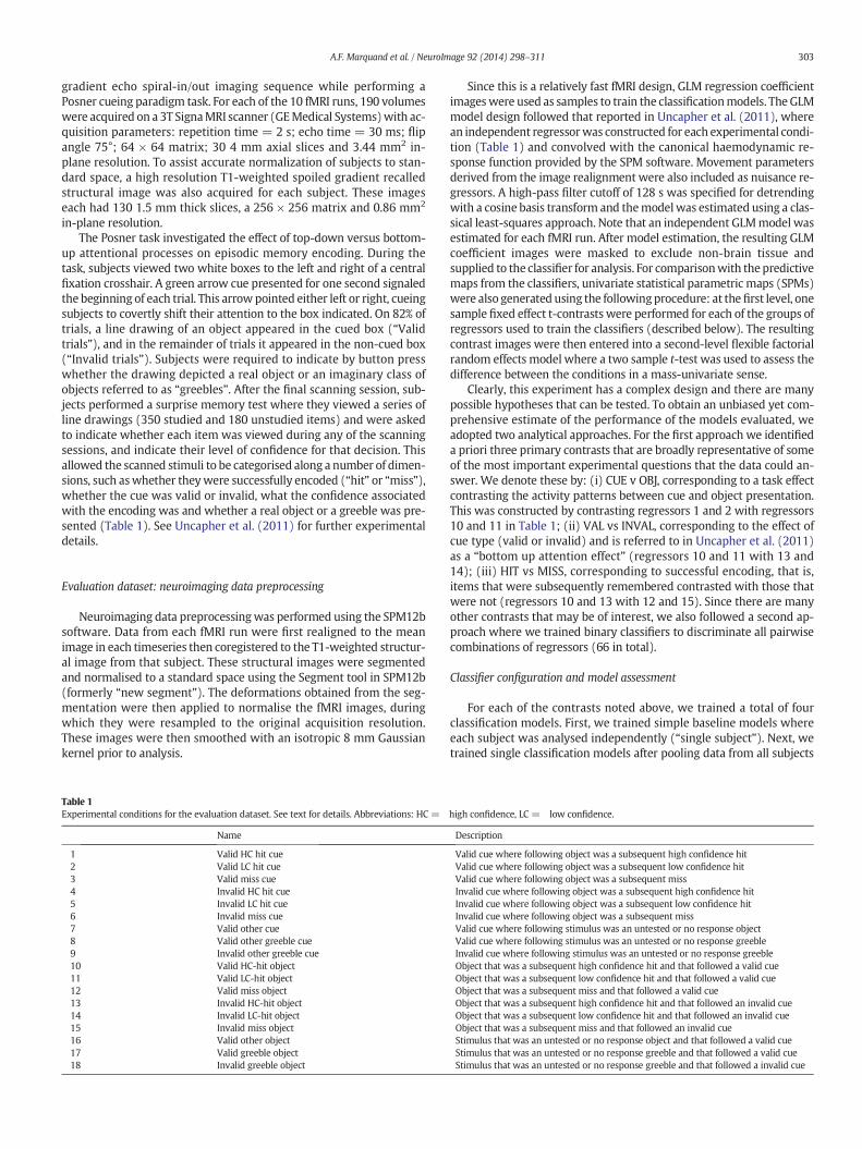
Table 1Experimental conditions for the evaluation dataset. See text for details. Abbreviations: HC =

Name

1 Valid HC hit cue2 Valid LC hit cue3 Valid miss cue4 Invalid HC hit cue5 Invalid LC hit cue6 Invalid miss cue7 Valid other cue8 Valid other greeble cue9 Invalid other greeble cue10 Valid HC-hit object11 Valid LC-hit object12 Valid miss object13 Invalid HC-hit object14 Invalid LC-hit object15 Invalid miss object16 Valid other object17 Valid greeble object18 Invalid greeble object

Since this is a relatively fast fMRI design, GLM regression coefficientimageswere used as samples to train the classificationmodels. The GLMmodel design followed that reported in Uncapher et al. (2011), wherean independent regressorwas constructed for each experimental condi-tion (Table 1) and convolved with the canonical haemodynamic re-sponse function provided by the SPM software. Movement parametersderived from the image realignment were also included as nuisance re-gressors. A high-pass filter cutoff of 128 s was specified for detrendingwith a cosine basis transform and themodelwas estimated using a clas-sical least-squares approach. Note that an independent GLMmodel wasestimated for each fMRI run. After model estimation, the resulting GLMcoefficient images were masked to exclude non-brain tissue andsupplied to the classifier for analysis. For comparisonwith thepredictivemaps from the classifiers, univariate statistical parametric maps (SPMs)were also generated using the followingprocedure: at thefirst level, onesample fixed effect t-contrasts were performed for each of the groups ofregressors used to train the classifiers (described below). The resultingcontrast images were then entered into a second-level flexible factorialrandom effects model where a two sample t-test was used to assess thedifference between the conditions in a mass-univariate sense.

Clearly, this experiment has a complex design and there are manypossible hypotheses that can be tested. To obtain an unbiased yet com-prehensive estimate of the performance of the models evaluated, weadopted two analytical approaches. For the first approach we identifieda priori three primary contrasts that are broadly representative of someof the most important experimental questions that the data could an-swer. We denote these by: (i) CUE v OBJ, corresponding to a task effectcontrasting the activity patterns between cue and object presentation.This was constructed by contrasting regressors 1 and 2 with regressors10 and 11 in Table 1; (ii) VAL vs INVAL, corresponding to the effect ofcue type (valid or invalid) and is referred to in Uncapher et al. (2011)as a “bottom up attention effect” (regressors 10 and 11 with 13 and14); (iii) HIT vs MISS, corresponding to successful encoding, that is,items that were subsequently remembered contrasted with those thatwere not (regressors 10 and 13 with 12 and 15). Since there are manyother contrasts that may be of interest, we also followed a second ap-proach where we trained binary classifiers to discriminate all pairwisecombinations of regressors (66 in total).

Classifier configuration and model assessment

For each of the contrasts noted above, we trained a total of fourclassification models. First, we trained simple baseline models whereeach subject was analysed independently (“single subject”). Next, wetrained single classification models after pooling data from all subjects

high confidence, LC = low confidence.

Description

Valid cue where following object was a subsequent high confidence hitValid cue where following object was a subsequent low confidence hitValid cue where following object was a subsequent missInvalid cue where following object was a subsequent high confidence hitInvalid cue where following object was a subsequent low confidence hitInvalid cue where following object was a subsequent missValid cue where following stimulus was an untested or no response objectValid cue where following stimulus was an untested or no response greebleInvalid cue where following stimulus was an untested or no response greebleObject that was a subsequent high confidence hit and that followed a valid cueObject that was a subsequent low confidence hit and that followed a valid cueObject that was a subsequent miss and that followed a valid cueObject that was a subsequent high confidence hit and that followed an invalid cueObject that was a subsequent low confidence hit and that followed an invalid cueObject that was a subsequent miss and that followed an invalid cueStimulus that was an untested or no response object and that followed a valid cueStimulus that was an untested or no response greeble and that followed a valid cueStimulus that was an untested or no response greeble and that followed a invalid cue

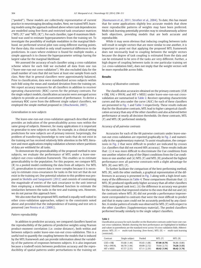
Table 2Classification accuracy for each classifier on the illustrative contrasts under leave-one-run-out cross-validation. Models showing the best performance are highlighted in boldfaceand values in parenthesis are the standard error across 10 cross-validation folds. Abbrevi-ations: MTL (F) = multi-task learning (free-form), MTL (R) = multi-task learning(restricted).

Contrast Single subject Pooled MTL (F) MTL (R)

CUE v OBJ 93.68 (1.44) 95.65 (1.08) 97.00 (0.79) 96.86 (0.80)VAL v INVAL 66.70 (1.94) 69.09 (2.72) 70.64 (2.73) 74.26 (1.55)HIT v MISS 67.57 (2.55) 67.11 (2.39) 68.42 (1.94) 68.42 (1.74)


(“pooled”). These models are collectively representative of currentpractice in neuroimaging decoding studies. Next, we trainedMTL learn-ingmodels using the approach outlined abovewhere task dependenciesare modelled using free-form and restricted task covariance matrices(“MTL (F)” and “MTL (R)”). For each classifier, type-II maximum likeli-hood was used to estimate hyperparameters from the training set. Toinvestigate the possibility of multiple modalities in the marginal likeli-hood, we performed several pilot runs using different starting points.For these data, this resulted in only small numerical differences to thepredictions. In cases where evidence is found for multiple modes, asimple approach is to choose the hyperparameter settings having thelargest value for the marginal likelihood.

We assessed the accuracy of each classifier using a cross-validationscheme where for each fold we excluded all data from one run(“leave-one-run-out cross-validation”). We also excluded data for thesmall number of runs that did not have at least one sample from eachclass. Note that in general classifiers were approximately balanced.Prior to classification, data were standardized across subjects withineach fold using the mean and standard deviation from the training set.We report accuracy measures for all classifiers in addition to receiveroperating characteristic (ROC) curves for the primary contrasts. Forthe single subjectmodels, classification accuracieswere averaged acrosssubjects to provide an overall assessment of performance. To derive asummary ROC curve from the different single subject classifiers, weemployed the simple method proposed in (Obuchowski, 2007).

Generalisation to new subjects

The leave-one-run-out cross-validation approach described aboveprovides an indication of the generalizability across runs within thesame group of subjects. However, for many applications it is importantto generalise to new subjects or tasks. For example, in a clinical settingpredictions for new subjects are of primary interest. Surprisingly, theproblem of transferring knowledge to new tasks that do not exist inthe training set has received relatively little attention in the MTL litera-ture andmost applications employ validation schemeswhere partitionsof data are withheld for all tasks.

To demonstrate the generalizability of the proposed method to newsubjects, we evaluate the performance of MTL under a leave-one-subject-out cross-validation framework. This enables us to estimategeneralizability to the population. For this purpose, we compare MTL(R) to a pooled model combining the data from all subjects. For MTL(F), generalisation to unseen data is more complex because it is neces-sary to estimate cross-covariances for tasks in the test set that do notexist in the training set. One potential solution to this problemwas pro-posed in Skolidis and Sanguinetti (2012) and consists of constrainingthe magnitude of entries of the task covariance to the unit intervalthen employing a multinomial likelihood function to estimate thesimilarities between the tasks in the test and training sets. However,we do not pursue this approach here.

We also note that the proposedMTLmethod is equallywell suited toother cross-validation approaches, subject to the constraints notedabove and provided that the independence of training and test sets ispreserved (see Pereira et al. (2009)).

Pattern reproducibility

In addition to predictive accuracy, we compared classifiers based onthe reproducibility of the patterns of predictive weights using Pearsonproduct-moment correlation (i.e. cosine distance), both within andbetween subjects under leave-one-run-out cross-validation. This is auseful tool to quantify the coupling between the models that is inducedby the MTL framework and can provide information about the variabil-ity of the patterns of responses between subjects. It is also importantbecause a tradeoff exists between prediction accuracy and the repro-ducibility of spatial patterns under perturbations to the training set

(Rasmussen et al., 2011; Strother et al., 2004). To date, this has meantthat for some applications slightly less accurate models that showmore reproducible patterns of weights may have been preferred.Multi-task learning potentially provides way to simultaneously achieveboth objectives, providing models that are both accurate andreproducible.

While it may seem obvious that inducing coupling between taskswill result in weight vectors that are more similar to one another, it isimportant to point out that applying the proposed MTL frameworkdoes not necessarily lead to coupling between the weight vectorsbecause the degree of task coupling is estimated from the data andcan be estimated to be zero if the tasks are very different. Further, ahigh degree of coupling between tasks in one particular training set(i.e. cross-validation fold), does not imply that the weight vectors willbe more reproducible across folds.

Results

Accuracy of illustrative contrasts

The classification accuracies obtained on the primary contrasts (CUEv OBJ, VAL v INVAL and HIT v MISS) under leave-one-run-out cross-validation are summarised in Table 2. Receiver operating characteristiccurves and the area under the curve (AUC) for each of these classifiersare presented in Fig. 1 and Table 3 respectively. These results indicatethat for the illustrative contrasts, MTL lead to higher categorical classifi-cation accuracy than any of the other classifiers and also achieved betterperformance at nearly all decision thresholds. On these contrasts, MTL(F) and MTL (R) performed similarly.

Accuracy of all pairwise contrasts

Accuracies for each of the 66 pairwise contrasts under leave-one-run-out cross-validation are reported graphically in Fig. 2 and numeri-cally in the supplementary material. To assist visualisation, the compar-isons in Fig. 2 that were difficult to predict are indicated by crosses(i.e. classifiers that did not exceed 60% accuracy). These results indicatethat: (i) it was more difficult to discriminate the Cue conditions fromone another relative of any of the Object conditions from the Cue condi-tions or one another and (ii) MTL (F) andMTL (R) produced the highestperformance over all pairwise constrasts with a slight advantage forMTL (R) over MTL (F).

To further facilitate the comparison of the best-performing method,MTL (R), with the other methods, a graphical representation of the dif-ferences in accuracy is presented in Fig. 3 along with a high-level sum-mary of the differences in Table 4. These comparisons illustrate that: (i)MTL (R) produced significantly higher accuracy than all other classifiers(Wilcoxon signed rank test); (ii) the difference in accuracy was greaterfor the contrasts that improved relative to the ones that did not and (iii)the contrasts where MTL (R) did not provide a performance improve-ment corresponded to contrasts that were the most difficult to predictand that in many cases could not be accurately predicted by any classi-fier. A similar pattern of resultswas observed forMTL (F)with respect tothe other classifiers (Supplementary material). The pooled classifiersperformed broadly similarly to the single subject classifiers.

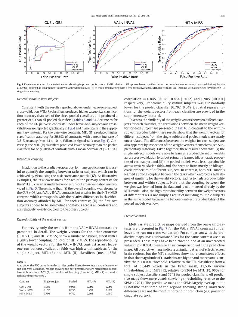
Fig. 1.Receiver operating characteristic curves showing improvedperformance ofMTL relative to STL approaches on the illustrative contrasts (leave-one-run-out cross-validation). For theCUE v OBJ contrast an enlargement is shown. Abbreviations: MTL (F) =multi-task learning with a free-form covariance, MTL (R)=multi-task learning with a restricted covariance, STL:single task learning.


Generalisation to new subjects

Consistent with the results reported above, under leave-one-subjectcross-validationMTL (R) classifiers produced higher categorical classifica-tion accuracy than two of the three pooled classifiers and produced agreater AUC than all pooled classifiers (Tables 5 and 6). Accuracies foreach of the 66 pairwise contrasts under leave-one-subject-out cross-validation are reported graphically in Fig. 4 andnumerically in the supple-mentary material. For the pair-wise contrasts, MTL (R) produced higherclassification accuracy for 89.39% of contrasts, with a mean increase of3.81% accuracy (p= 1.1 × 10−7, Wilcoxon signed rank test; Fig. 4). Con-versely, the MTL (R) classifiers produced lower accuracy than the pooledclassifiers for only 9.09% of contrasts with a mean decrease of (−1.15%).

Inter-task coupling

In addition to the predictive accuracy, formany applications it is use-ful to quantify the coupling between tasks or subjects, which can beachieved by visualising the task covariance matrix (Kf). As illustrativeexamples, the task covariances for each of the primary contrasts fortheMTL (F) classifier under leave-one-run-out cross-validation are pro-vided in Fig. 5. These show that: (i) the overall coupling was strong forthe CUE v OBJ and VAL v INVAL contrasts but weaker for the HIT v MISScontrast, which corresponds with the relative differences in classifica-tion accuracy afforded by MTL for each contrast; (ii) the first twosubjects appear to be somewhat anomalous across all contrasts andare relatively weakly coupled to the other subjects.

Reproducibility of the weight vectors

For brevity, only the results from the VAL v INVAL contrast arepresented in detail. The weight vectors for the other contrasts(CUE v OBJ and HIT v MISS) show a similar behaviour, albeit with aslightly lower coupling induced for HIT v MISS. The reproducibilityof the weight vectors for the VAL v INVAL contrast across leave-one-run-out cross-validation folds was high within subjects for thesingle subject, MTL (F) and MTL (R) classifiers (mean [SEM]

Table 3Area under the ROC curve for each classifier on the illustrative contrasts under leave-one-run-out cross validation. Models showing the best performance are highlighted in bold-face. Abbreviations: MTL (F) = multi-task learning (free-form), MTL (R) = multi-task learning (restricted).

Contrast Single subject Pooled MTL (F) MTL (R)

CUE v OBJ 0.995 0.996 0.999 0.999VAL v INVAL 0.657 0.755 0.793 0.820HIT v MISS 0.706 0.702 0.764 0.750

correlation = 0.845 [0.028], 0.834 [0.012] and 0.905 [b0.001]respectively). Reproducibility within subjects was substantiallylower for the pooled classifier (0.702 [0.048]). Spatial representa-tions for the weight vectors from each classifier are provided in thesupplementary material.

To assess the similarity of the weight vectors between different sub-jects for each classifier, the correlations between the mean weight vec-tor for each subject are presented in Fig. 6. In contrast to the within-subject reproducibility, these results show that the weight vectors fordifferent subjects from the single subject and pooled models are nearlyuncorrelated. The differences between the weights for each subject arealso apparent by inspection of the weight vectors themselves (see Sup-plementary material). Taken together, these results show that: (i) thesingle subject models were able to learn a reproducible set of weightsacross cross-validation folds but primarily learned idiosyncratic proper-ties of each subject and (ii) the pooled models were less reproducibleacross cross-validation folds, and also seem to focus mostly on idiosyn-cratic properties of different subjects. In contrast, both MTL modelslearned a strong coupling between the tasks which enforced a high de-gree of similarity for the weight vectors, leading to high reproducibilitybetween and within subjects. Note that the coupling between theweights was learned from the data and is not imposed directly by theMTL model. Also, the high reproducibility between the weight vectorsof different tasks is not simply a result of including multiple subjectsin the same model, because the between-subject reproducibility of thepooled models was low.

Predictive maps

Multivariate predictive maps derived from the one-sample t-tests are presented in Fig. 7 for the VAL v INVAL contrast (underleave-one-run-out cross-validation). For comparison with the pre-dictive maps, mass-univariate SPMs for the same contrast are alsopresented. These maps have been thresholded at an uncorrectedvalue of p b 0.001 to ensure a fair comparison with the predictivemaps. All predictive maps indicate a similar pattern of effects acrossbrain regions, but the MTL classifiers show more consistent effectsin that the magnitude of t-statistics are higher and more voxels sur-vive the p b 0.001 threshold, relative to the STL classifiers; from atotal of 35,449 voxels in the brain mask, 11,536 survivethresholding in for MTL (R), relative to 9264 for MTL (F), 6662 forsingle subject classifiers and 5743 for pooled classifiers. All predic-tive maps show more voxels surviving thresholding relative to theSPMs (2704). The predictive maps and SPMs largely overlap, but itis notable that some of the regions showing strong univariatedifferences are not the most important for prediction (e.g. posteriorcingulate cortex).

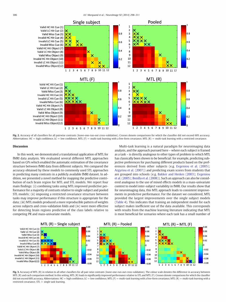
Fig. 2. Accuracy of all classifiers for all pairwise contrasts (leave-one-run-out cross-validation). Crosses denote comparisons for which the classifier did not exceed 60% accuracy.Abbreviations: HC = high confidence, LC = low confidence, MTL (F) = multi-task learning with a free-form covariance, MTL (R) = multi-task learning with a restricted covariance.


Discussion

In this work, we demonstrated a translational application of MTL forfMRI data analysis. We evaluated several different MTL approachesbased on GPswhich enabled the automatic estimation of the covariancestructure between fMRI data from different subjects. We compared theaccuracy obtained by these models to commonly used STL approachesin predicting many contrasts in a publicly available fMRI dataset. In ad-dition, we presented a novel method for mapping the predictive contri-bution of each brain region for MTL and STL models. We report fourmain findings: (i) combining tasks using MTL improved predictive per-formance for amajority of contrasts relative to single subject and pooledSTL models; (ii) imposing a restricted covariance structure betweentasks may improve performance if this structure is appropriate for thedata; (iii)MTLmodels produced amore reproducible pattern ofweightsacross subjects and cross-validation folds and (iv) were more effectivefor detecting brain regions predictive of the class labels relative tocompeting PR and mass-univariate models.

Fig. 3. Accuracy of MTL (R) in relation to all other classifiers for all pair-wise contrasts (leave-oMTL (R) and each comparisonmethod. In this setting,MTL (R) leads to significantly improved pedid not exceed60% accuracy. Abbreviations: HC=high confidence, LC= low confidence,MTL (restricted covariance, STL = single task learning.

Multi-task learning is a natural paradigm for neuroimaging dataanalysis, and the approach pursued here –where each subject is framedas a task – is directly analogous to other types of problem to whichMTLhas classically been shown to be beneficial: for example, predicting sub-jective preferences for purchasing different products based on the pref-erences derived from other subjects (e.g. Evgeniou et al. (2005);Argyriou et al. (2007)) and predicting exam scores from students thatare grouped into schools (e.g. Bakker and Heskes (2003); Evgeniouet al. (2005); Bonilla et al. (2008)). Such an approach can also be consid-ered analogous to the use of mixed effects models in a mass-univariatecontext to model inter-subject variability in fMRI. Our results show thatfor neuroimaging data, this MTL approach leads to consistent improve-ments in predictive performance. For the dataset we considered, MTLprovided the largest improvements over the single subject models(Table 4). This indicates that training an independent model for eachsubject makes inefficient use of the data available. This correspondswith results from the machine learning literature indicating that MTLis most beneficial for scenarios where each task has a small number of

ne-run-out cross-validation). The colour scale denotes the difference in accuracy betweenrformance relative to STL andMTL (F). Crosses denote comparisons forwhich the classifierF)=multi-task learningwith a free-form covariance,MTL (R)=multi-task learningwith a

image of Fig.�2

image of Fig.�3

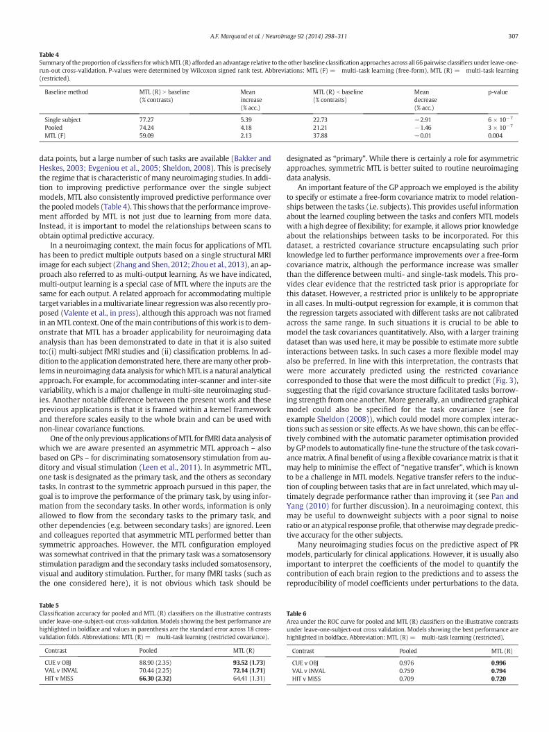
Table 4Summary of the proportion of classifiers forwhichMTL (R) afforded an advantage relative to the other baseline classification approaches across all 66 pairwise classifiers under leave-one-run-out cross-validation. P-values were determined by Wilcoxon signed rank test. Abbreviations: MTL (F) = multi-task learning (free-form), MTL (R) = multi-task learning(restricted).

Baseline method MTL (R) N baseline(% contrasts)

Meanincrease(% acc.)

MTL (R) b baseline(% contrasts)

Meandecrease(% acc.)

p-value

Single subject 77.27 5.39 22.73 −2.91 6 × 10−7

Pooled 74.24 4.18 21.21 −1.46 3 × 10−7

MTL (F) 59.09 2.13 37.88 −0.01 0.004


data points, but a large number of such tasks are available (Bakker andHeskes, 2003; Evgeniou et al., 2005; Sheldon, 2008). This is preciselythe regime that is characteristic of many neuroimaging studies. In addi-tion to improving predictive performance over the single subjectmodels, MTL also consistently improved predictive performance overthe pooledmodels (Table 4). This shows that the performance improve-ment afforded by MTL is not just due to learning from more data.Instead, it is important to model the relationships between scans toobtain optimal predictive accuracy.

In a neuroimaging context, the main focus for applications of MTLhas been to predict multiple outputs based on a single structural MRIimage for each subject (Zhang and Shen, 2012; Zhou et al., 2013), an ap-proach also referred to as multi-output learning. As we have indicated,multi-output learning is a special case of MTL where the inputs are thesame for each output. A related approach for accommodating multipletarget variables in amultivariate linear regressionwas also recently pro-posed (Valente et al., in press), although this approach was not framedin anMTL context. One of themain contributions of this work is to dem-onstrate that MTL has a broader applicability for neuroimaging dataanalysis than has been demonstrated to date in that it is also suitedto:(i) multi-subject fMRI studies and (ii) classification problems. In ad-dition to the application demonstrated here, there aremany other prob-lems in neuroimaging data analysis for whichMTL is a natural analyticalapproach. For example, for accommodating inter-scanner and inter-sitevariability, which is a major challenge in multi-site neuroimaging stud-ies. Another notable difference between the present work and theseprevious applications is that it is framed within a kernel frameworkand therefore scales easily to the whole brain and can be used withnon-linear covariance functions.

One of the only previous applications ofMTL for fMRI data analysis ofwhich we are aware presented an asymmetric MTL approach – alsobased on GPs – for discriminating somatosensory stimulation from au-ditory and visual stimulation (Leen et al., 2011). In asymmetric MTL,one task is designated as the primary task, and the others as secondarytasks. In contrast to the symmetric approach pursued in this paper, thegoal is to improve the performance of the primary task, by using infor-mation from the secondary tasks. In other words, information is onlyallowed to flow from the secondary tasks to the primary task, andother dependencies (e.g. between secondary tasks) are ignored. Leenand colleagues reported that asymmetric MTL performed better thansymmetric approaches. However, the MTL configuration employedwas somewhat contrived in that the primary task was a somatosensorystimulation paradigm and the secondary tasks included somatosensory,visual and auditory stimulation. Further, for many fMRI tasks (such asthe one considered here), it is not obvious which task should be

Table 5Classification accuracy for pooled and MTL (R) classifiers on the illustrative contrastsunder leave-one-subject-out cross-validation. Models showing the best performance arehighlighted in boldface and values in parenthesis are the standard error across 18 cross-validation folds. Abbreviations: MTL (R) = multi-task learning (restricted covariance).

Contrast Pooled MTL (R)

CUE v OBJ 88.90 (2.35) 93.52 (1.73)VAL v INVAL 70.44 (2.25) 72.14 (1.71)HIT v MISS 66.30 (2.32) 64.41 (1.31)

designated as “primary”. While there is certainly a role for asymmetricapproaches, symmetric MTL is better suited to routine neuroimagingdata analysis.

An important feature of the GP approach we employed is the abilityto specify or estimate a free-form covariance matrix to model relation-ships between the tasks (i.e. subjects). This provides useful informationabout the learned coupling between the tasks and confers MTL modelswith a high degree of flexibility; for example, it allows prior knowledgeabout the relationships between tasks to be incorporated. For thisdataset, a restricted covariance structure encapsulating such priorknowledge led to further performance improvements over a free-formcovariance matrix, although the performance increase was smallerthan the difference between multi- and single-task models. This pro-vides clear evidence that the restricted task prior is appropriate forthis dataset. However, a restricted prior is unlikely to be appropriatein all cases. In multi-output regression for example, it is common thatthe regression targets associated with different tasks are not calibratedacross the same range. In such situations it is crucial to be able tomodel the task covariances quantitatively. Also, with a larger trainingdataset than was used here, it may be possible to estimate more subtleinteractions between tasks. In such cases a more flexible model mayalso be preferred. In line with this interpretation, the contrasts thatwere more accurately predicted using the restricted covariancecorresponded to those that were the most difficult to predict (Fig. 3),suggesting that the rigid covariance structure facilitated tasks borrow-ing strength from one another. More generally, an undirected graphicalmodel could also be specified for the task covariance (see forexample Sheldon (2008)), which could model more complex interac-tions such as session or site effects. Aswe have shown, this can be effec-tively combined with the automatic parameter optimisation providedby GPmodels to automatically fine-tune the structure of the task covari-ancematrix. A final benefit of using a flexible covariancematrix is that itmay help to minimise the effect of “negative transfer”, which is knownto be a challenge in MTL models. Negative transfer refers to the induc-tion of coupling between tasks that are in fact unrelated, whichmay ul-timately degrade performance rather than improving it (see Pan andYang (2010) for further discussion). In a neuroimaging context, thismay be useful to downweight subjects with a poor signal to noiseratio or an atypical response profile, that otherwisemaydegrade predic-tive accuracy for the other subjects.

Many neuroimaging studies focus on the predictive aspect of PRmodels, particularly for clinical applications. However, it is usually alsoimportant to interpret the coefficients of the model to quantify thecontribution of each brain region to the predictions and to assess thereproducibility of model coefficients under perturbations to the data.

Table 6Area under the ROC curve for pooled and MTL (R) classifiers on the illustrative contrastsunder leave-one-subject-out cross validation. Models showing the best performance arehighlighted in boldface. Abbreviation: MTL (R) = multi-task learning (restricted).

Contrast Pooled MTL (R)

CUE v OBJ 0.976 0.996VAL v INVAL 0.759 0.794HIT v MISS 0.709 0.720

Fig. 4. Top panels: Accuracy of MTL (R) and pooled classifiers for all pairwise contrasts (leave-one-subject-out cross-validation). Bottom panel: difference between MTL (R) and pooledclassifiers (leave-one-subject-out cross-validation). In this setting, MTL (R) leads to significantly improved performance relative to pooled classifiers. Crosses denote comparisons forwhich the classifier did not exceed 60% accuracy. Abbreviations: HC = high confidence, LC = low confidence, MTL (R) = multi-task learning with a restricted covariance.


This is most commonly done by mapping the classifier weight vector inthe voxel space (e.g. Mourao-Miranda et al. (2005); Kloppel et al.(2008); Marquand et al. (2012); Gaonkar and Davatzikos (2012)).Since the weights alone do not determine the contribution of eachvoxel to the prediction, we propose to take this approach a step furtherbymapping the product of the weights and the data at each brain voxel.This “predictive mapping” approach is applicable to many of types ofclassifier employed in neuroimaging (e.g. support vector machinesand penalised linearmodels) and yields twomain benefits: (i) it is intu-itively appealing in that it quantifies the total contribution of what wasactually used tomake predictions at each brain voxel and (ii) it lends it-self naturally to a statistical approach to assess the predictive contribu-tion of different brain regions. In theVALv INVAL contrastwe examined,the MTL models induced strong coupling between the tasks (i.e. sub-jects). As expected, this resulted in high within- and between subject

Fig. 5.Hinton diagram showing examples of task covariancematrices for each of the primary cothe covariances from the first leave-one-run-out cross-validation fold. Abbreviation: MTL (F) =

reproducibility in the patterns of discriminative weights. In contrast,single-subject and pooled classification approaches yielded discrimina-tive patterns that were either inconsistent across subjects or thatshowed poor reproducibility across cross-validation folds. This in turnled to an increase in both the magnitude of t-statistics and the numberof voxels surviving an arbitrary but commonly used threshold in thepredictive maps for the MTL- relative to STL models (Fig. 7). All PR ap-proaches detectedmore significant voxels than a comparable univariateSPM, which provides an indication of the utility of predictive mappingfor detecting spatially distributed effects. However, it is important tonote that the SPMs and predictive maps have a different interpretation:the SPMs describe focal, group level effects; the predictive maps sum-marise the total contribution of each brain region to predicting theclass labels at the single subject level. Correspondingly, the regionswith a large group-level difference are not necessarily the same as

ntrasts. This illustrates the inter-task coupling learned by theMTL (F) classifiers. Shown aremulti-task learning with a free-form covariance.

image of Fig.�4

image of Fig.�5

Fig. 6.Hinton diagram showing the correlations between theweight vectors for each subject and classifier. This shows that bothMTL approaches lead tomore reproducibleweight vectors.Abbreviation: MTL (F) = multi-task learning with a free-form covariance, MTL (R) = multi-task learning with a restricted covariance.


those that are most useful for prediction. Another important caveat tothe foregoing is that the degree of regularisation employed also influ-ences the reproducibility of the spatial patterns (Rasmussen et al.,2011), so we cannot exclude the possibility that different degrees ofregularisation between single- andmulti- task learningmodels contrib-uted to their differential effects. To investigate this, we repeated the STLanalysis using a range of different regularisation strengths with the co-variance function described in (Marquand et al., 2010), and obtainednearly identical results, which would seem to eliminate this possibility.

We argue that by accommodating inter-subject variations as differ-ent tasks and searching for commonalities between subjects, MTLmodels are better able to capture the consistent discriminative patternacross the group relative to the corresponding single-task models.This consensus pattern is usually what is of primary interest in multi-subject neuroimaging studies, and is probably responsible for the im-provement in accuracy provided byMTL over STLmodels. This rationalealso bears similarities with recent work that aims to select themost sta-ble features for decoding cognitive states (Gramfort et al., 2011;Rondina et al., 2014; Ryali et al., 2012). In general, the magnitude ofthe improvement provided by coupling the subjects through MTL islikely to be dependent on the particular application and the nature ofthe pattern of responses elicited by the fMRI task. This is because thefunctional anatomy in some brain regions (e.g. frontal eye fields) iswell aligned to cortical structures whereas the anatomical locations of

other highly specialised regions (e.g. fusiform face area) are more vari-able across subjects, even after subjects have beenwell aligned structur-ally (Frost and Goebel, 2012). Similarly, the degree of spatial smoothingapplied to the datamay influence the similarity of the images belongingto different subjects. However, it is important to point out that the pro-posed method is still able to accommodate the settings where variabil-ity between subjects is high or the smoothing is not optimal by reducingthe coupling induced between the tasks.

In this work, we framed the MTL problem in the context ofGP models, which have desirable properties for neuroimaging (e.g.probabilistic predictions and the ability to automatically tune modelhyperparameters using type-II maximum likelihood). Another impor-tant motivation for our choice of method was the scalability of themethod to whole-brain voxel-wise data and large numbers of tasks.We expect that many of the benefits of MTL models we have demon-strated are not limited to GPs and may generalise to different MTLapproaches. For further work, it would be interesting to evaluateapproaches that confer different benefits, such as structured sparsity(e.g. Michel et al. (2011); Grosenick et al. (2013); Sohn and Kim(2012); Marquand et al. (2013a)). However, an important point tobear in mind is that for MTL it is necessary to estimate a large numberof weight vectors (at least one per task). This may become problematicif the analytical method scales according to the dimensionality of theinput space, as is often the case for sparse models. In contrast, the

image of Fig.�6

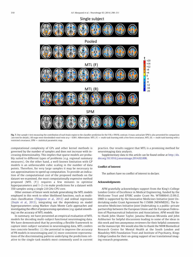
Fig. 7. One sample t-test measuring the contribution of each brain region to the classifier prediction for the VAL v INVAL contrast. A mass-univariate SPM is also presented for comparison(see text for details). All maps were thresholded voxel-wise at p b 0.001. Abbreviation: MTL (F) =multi-task learning with a free form covariance, MTL (R) =multi-task learningwith arestricted covariance, SPM = statistical parametric map.


computational complexity of GPs and other kernel methods isgoverned by the number of samples and does not increase with in-creasing dimensionality. This implies that sparse models are proba-bly suited to different types of problems (e.g. regional summarymeasures). On the other hand, a well-known limitation with GPmodels is an unfavourable cubic scaling in the number of datapoints. Therefore, for very large samples it may be necessary touse approximations to speed up computation. To provide an indica-tion of the computational cost of the proposed methods on thedataset we examined, the most computationally expensive methodproposed (MTL (F)) requires a few minutes to optimisehyperparameters and 1–2 s to make predictions for a dataset with350 samples using a single 2.8 GHz CPU core.

Other avenues of future work include generalising the MTL modelsemployed in this work to other likelihood functions, such as multi-class classification (Filippone et al., 2012) and ordinal regression(Doyle et al., 2013), integrating out the dependency on modelhyperparameters using Markov chain Monte Carlo approaches andinvestigating the effect of preprocessing operations (e.g. spatial smooth-ing) on the accuracy of MTL models.

In summary, we have presented an empirical evaluation of MTLmodels for decoding multi-subject functional neuroimaging data.We have demonstrated that by providing a flexible framework tocapture inter-subject variation in neuroimaging data, MTL conferstwo concrete benefits: (i) the potential to improve the accuracyof PR models in neuroimaging and (ii) more consistent representa-tions of the discriminating patterns underlying the predictions rel-ative to the single-task models most commonly used in current

practice. Our results suggest that MTL is a promising method forneuroimaging data analysis.

Supplementary data to this article can be found online at http://dx.doi.org/10.1016/j.neuroimage.2014.02.008.

Conflict of Interest

The authors have no conflict of interest to declare.

Acknowledgments

AFM gratefully acknowledges support from the King's CollegeLondon Centre of Excellence in Medical Engineering, funded by theWellcome Trust and EPSRC under Grant No. WT088641/Z/09/Z.OMD is supported by the Innovative Medicines Initiative Joint Un-dertaking under Grant Agreement No 115008 (NEWMEDS). The In-novative Medicines Initiative Joint Undertaking is a public–privatepartnership between the European Union and the European Federa-tion of Pharmaceutical Industries and Associations. AFM would liketo thank John Shawe Taylor, Janaina Mourao-Miranda and JohnAshburner for helpful discussions leading to some of the ideas inthis work and two anonymous reviewers for their helpful commentson the manuscript. We would also like to thank the NIHR BiomedicalResearch Centre for Mental Health at the South London andMaudsley NHS Foundation Trust and Institute of Psychiatry, KingsCollege London for their on-going support of our translational imag-ing research programme.



image of Fig.�7


References

Abernethy, J., Bach, F., Evgeniou, T., Vert, J.P., 2009. A new approach to collaborative filter-ing: operator estimation with spectral regularization. J. Mach. Learn. Res. 10,803–826.

Aguirre, G.K., Zarahn, E., D'Esposito, M., 1998. The variability of human, bold hemodynam-ic responses. NeuroImage 8, 360–369.

Alvarez, M.A., Lawrence, N.D., 2008. Sparse convolved Gaussian processes for multi-output regression. In: Koller, D., Schuurmans, D., Bengio, Y., Bottou, L. (Eds.), NIPS.Curran Associates, Inc., pp. 57–64.

Argyriou, A., Evgeniou, T., Pontil, M., 2007. Multi-task feature learning. Advances in NeuralInformation Processing Systems, 19. MIT Press, pp. 41–48.

Bakker, B., Heskes, T., 2003. Task clustering and gating for Bayesian multitask learning.J. Mach. Learn. Res. 4, 2003.

Bishop, C., 2006. Pattern Recognition and Machine Learning. Springer, New York.Bonilla, E.V., Chai, K.M., Williams, C.K.I., 2008. Multi-task Gaussian process prediction. In:

Platt, J.C., Koller, D., Singer, Y., Roweis, S. (Eds.), Advances in Neural InformationProcessing Systems, 20. MIT Press, Cambridge, MA, pp. 153–160.

Boyle, P., Frean, M., 2005. Dependent Gaussian processes. Advances in Neural InformationProcessing Systems, 17. MIT Press, pp. 217–224.

Brodersen, K.H., Wiech, K., Lomakina, E.I., shu Lin, C., Buhmann, J.M., Bingel, U., Ploner, M.,Stephan, K.E., Tracey, I., 2012. Decoding the perception of pain from fmri usingmultivariate pattern analysis. NeuroImage 63, 1162–1170.

Caruana, R., 1997. Multitask learning. Mach. Learn. 28, 41–75.Cressie, N., 1993. Statistics for spatial data. Wiley series in probability and mathematical

statistics: applied probability and statistics. J. Wiley.Doyle, O., Ashburner, J., Zelaya, F., Williams, S., Mehta, M., Marquand, A., 2013. Multivar-

iate decoding of brain images using ordinal regression. NeuroImage 81, 347–357.Evgeniou, T., Micchelli, C.A., Pontil, M., 2005. Learningmultiple taskswith kernel methods.

J. Mach. Learn. Res. 6, 615–637.Filippone, M., Marquand, A., Blain, C., Williams, S., Mourao-Miranda, J., Girolami, M., 2012.

Probabilistic prediction of neurological disorders with a statistical assessment ofneuroimaging data modalities. Ann. Appl. Stat. 6, 1883–1905.

Friston, K.J., Frith, C.D., Frackowiak, R.S., Turner, R., 1995. Characterizing dynamic brainresponses with fMRI: a multivariate approach. NeuroImage 2, 166–172.

Friston, K., Stephan, K., Lund, T., Morcom, A., Kiebel, S., 2005. Mixed-effects and fMRIstudies. NeuroImage 24, 244–252.

Frost, M.A., Goebel, R., 2012. Measuring structural and functional correspondence: spatialvariability of specialised brain regions after macro-anatomical alignment.NeuroImage 59, 1369–1381. http://dx.doi.org/10.1016/j.neuroimage.2011.08.035.

Gaonkar, B., Davatzikos, C., 2012. Deriving statistical significance maps for svm basedimage classification and group comparisons. Proceedings of the 15th InternationalConference on Medical Image Computing and Computer-Assisted Intervention —

Volume Part I. Springer-Verlag, Berlin, Heidelberg, pp. 723–730.Gramfort, A., Varoquaux, G., Thirion, B., 2011. Beyond brain reading: randomized sparsity

and clustering to simultaneously predict and identify. In: Langs, G., Rish, I., Grosse-Wentrup, M., Murphy, B. (Eds.), MLINI. Springer, pp. 9–16.

Grosenick, L., Greer, S., Knutson, B., 2008. Interpretable classifiers for fMRI improveprediction of purchases. IEEE Trans. Neural Syst. Rehabil. Eng. 16, 539–548.

Grosenick, L., Klingenberg, B., Katovich, K., Knutson, B., Taylor, J.E., 2013. Interpretablewhole-brain prediction analysis with Graphnet. NeuroImage 72, 304–321.

Handwerker, D.A., Ollinger, J.M., D'Esposito, M., 2004. Variation of bold hemodynamic re-sponses across subjects and brain regions and their effects on statistical analyses.NeuroImage 21, 1639–1651.

Hastie, T., Tibshirani, R., Buja, A., 1993. Flexible discriminant analysis by optimal scoring.J. Am. Stat. Assoc. 89, 1255–1270.

Hastie, T., Buja, A., Tibshirani, R., 1995. Penalized discriminant analysis. Ann. Stat. 23,73–102.

Holmes, A., Friston, K., 1998. Generalisability, random effects and population inference.NeuroImage 7, S754.

Kloppel, S., Stonnington, C.M., Chu, C., Draganski, B., Scahill, R.I., Rohrer, J.D., Fox, N.C., Jack,C.R., Ashburner, J., Frackowiak, R.S.J., 2008. Automatic classification of MR scans inAlzheimer's disease. Brain 131, 681–689.

Leen, G., Peltonen, J., Kaski, S., 2011. Focused multi-task learning using Gaussian process-es. In: Gunopulos, D., Hofmann, T., Malerba, D., Vazirgiannis, M. (Eds.), ECML/PKDD(2). Springer, pp. 310–325.

Marquand, A., Howard, M., Brammer, M., Chu, C., Coen, S., Mourao-Miranda, J., 2010.Quantitative prediction of subjective pain intensity from whole-brain fMRI datausing Gaussian processes. NeuroImage 49, 2178–2189.

Marquand, A., De Simoni, S., O'Daly, O., Williams, S., MourÃ£o-Miranda, J., Mehta, M.,2011. Pattern classification of working memory networks reveals differentialeffects of methylphenidate, atomoxetine, and placebo in healthy volunteers.Neuropsychopharmacology 36, 1237–1247.

Marquand, A.F., O'Daly, O.G., Simoni, S.D., Alsop, D.C., Maguire, R.P., Williams, S.C., Zelaya,F.O., Mehta, M.A., 2012. Dissociable effects of methylphenidate, atomoxetine andplacebo on regional cerebral blood flow in healthy volunteers at rest: a multi-classpattern recognition approach. NeuroImage 60, 1015–1024.

Marquand, A.F., Filippone, M., Ashburner, J., Girolami, M., Mourao-Miranda, J., Barker, G.J.,Williams, S.C.R., Leigh, P.N., Blain, C.R.V., 2013a. Automated, high accuracy

classification of parkinsonian disorders: a pattern recognition approach. PLoS ONE8, e69237.

Marquand, A., Rosa, M., Doyle, O., 2013b. Conditional Gaussian graphical models formulti-output regression of neuroimaging data. First International Workshop onRegularization, Optimization, Kernels and Support Vector Machines, Leuven,Belgium, pp. 81–82.

Meriaux, S., Roche, A., Dehaene-Lambertz, G., Thirion, B., Poline, J.B., 2006. Combinedpermutation test and mixed-effect model for group average analysis in fMRI. Hum.Brain Mapp. 27, 402–410.

Michel, V., Gramfort, A., Varoquaux, G., Eger, E., Thirion, B., 2011. Total variation regular-ization for fMRI-based prediction of behavior. IEEE Trans. Med. Imaging 30,1328–1340.

Minka, T., 2001. A Family of Algorithms for Approximate Bayesian Inference. (PhD thesis).Morosan, P., Rademacher, J., Schleicher, A., Amunts, K., Schormann, T., Zilles, K., 2001.

Human primary auditory cortex: cytoarchitectonic subdivisions and mapping into aspatial reference system. NeuroImage 13, 684–701.

Mourao-Miranda, J., Bokde, A.L., Born, C., Hampel, H., Stetter, M., 2005. Classifying brainstates and determining the discriminating activation patterns: support vectormachine on functional mri data. NeuroImage 28, 980–995.

Naselaris, T., Kay, K.N., Nishimoto, S., Gallant, J.L., 2011. Encoding and decoding in fMRI.NeuroImage 56, 400–410 (Multivariate Decoding and Brain Reading).

Nichols, T., Holmes, A., 2002. Nonparametric permutation tests for functional neuroimag-ing: a primer with examples. Hum. Brain Mapp. 15, 1–25.

Nickisch, H., Rasmussen, C.E., 2008. Approximations for binary Gaussian process classifi-cation. J. Mach. Learn. Res. 9, 2035–2078.

Norman, K.A., Polyn, S.M., Detre, G.J., Haxby, J.V., 2006. Beyondmind-reading: multi-voxelpattern analysis of fMRI data. Trends Cogn. Sci. 10, 424–430.

Obuchowski, N.A., 2007. New methodological tools for multiple-reader roc studies1.Radiology 243, 10–12.

Orru, G., Pettersson-Yeo, W., Marquand, A., Sartori, G., Mechelli, A., 2012. Using supportvector machine to identify imaging biomarkers of neurological and psychiatricdisease: a critical review. Neurosci. Biobehav. Rev. 36, 1140–1152.

Pan, S.J., Yang, Q., 2010. A survey on transfer learning. IEEE Trans. Knowl. Data Eng. 22,1345–1359.

Pereira, F., Mitchell, T., Botvinick, M., 2009. Machine learning classifiers and fMRI: atutorial overview. NeuroImage 45, S199–S209.

Rasmussen, C., Williams, C.K.I., 2006. Gaussian Processes for Machine Learning. The MITPress, Cambridge, Massachusetts.

Rasmussen, P.M., Hansen, L.K., Madsen, K.H., Churchill, N.W., Strother, S.C., 2011. Modelsparsity and brain pattern interpretation of classification models in neuroimaging.Pattern Recogn. 45, 2085–2100.

Rondina, J., Hahn, T., de Oliveira, L., Marquand, A., Dresler, T., Leitner, T., Fallgatter, A.,Shawe-Taylor, J., Mourao-Miranda, J., 2014. Scors: a method based on stability forfeature selection and mapping in neuroimaging. IEEE Trans. Med. Imaging 33,85–98.

Ryali, S., Chen, T., Supekar, K., Menon, V., 2012. Estimation of functional connectivity infMRI data using stability selection-based sparse partial correlation with elastic netpenalty. NeuroImage 59, 3852–3861.

Sheldon, D., 2008. Graphical multi-task learning. Technical Report.Skolidis, G., Sanguinetti, G., 2011. Bayesian multitask classification with Gaussian process

priors. IEEE Trans. Neural Networks 22, 2011–2021.Skolidis, G., Sanguinetti, G., 2012. A case study onmeta-generalising: a Gaussian processes

approach. J. Mach. Learn. Res. 13, 691–721.Sohn, K.A., Kim, S., 2012. Joint estimation of structured sparsity and output structure in

multiple-output regression via inverse-covariance regularization. J. Mach. Learn.Res. Proc. Track 22, 1081–1089.

Strother, S., La Conte, S., Hansen, L.K., Anderson, J., Zhang, J., Pulapura, S., Rottenberg, D., 2004.Optimizing the fMRI data-processing pipeline using prediction and reproducibility per-formance metrics: I. A preliminary group analysis. NeuroImage 23, S196–S207.

Uncapher, M.R., Hutchinson, J.B., Wagner, A.D., 2011. Dissociable effects of top-down andbottom-up attention during episodic encoding. J. Neurosci. 31, 12613–12628.

Valente, G., Castellanos, A.L., Vanacor, G., Formisano, E., 2014. Multivariate linear regres-sion of high-dimensional fMRI data with multiple target variables. Hum. BrainMapp. http://dx.doi.org/10.1002/hbm.22318 (in press).

Varoquaux, G., Gramfort, A., Poline, J.B., Thirion, B., 2010. Brain covariance selection:better individual functional connectivity models using population prior. In: Lafferty,J.D., Williams, C.K.I., Shawe-Taylor, J., Zemel, R.S., Culotta, A. (Eds.), NIPS. CurranAssociates, Inc., pp. 2334–2342.

Wang, Z., Childress, A.R., Wang, J.J., Detre, J.A., 2007. Support vector machine learning-based fMRI data group analysis. NeuroImage 36, 1139–1151 (Wang, Ze Childress,Anna R. Wang, Jiongjiong Detre, Jobn A.).

Woolrich, M.W., Behrens, T.E.J., Beckmann, C.F., Jenkinson, M., Smith, S.M., 2004. Multilev-el linear modelling for FMRI group analysis using Bayesian inference. NeuroImage 21,1732–1747.

Zhang, D., Shen, D., 2012. Multi-modal multi-task learning for joint prediction of multipleregression and classification variables in Alzheimer's disease. NeuroImage 59,895–907.

Zhou, J., Liu, J., Narayan, V.A., Ye, J., 2013. Modeling disease progression via multi-tasklearning. NeuroImage 78, 233–248.

http://refhub.elsevier.com/S1053-8119(14)00099-8/rf0005






























































































































http://dx.doi.org/10.1002/hbm.22318
















Bayesian multi-task learning for decoding multi-subject neuroimaging data

Documents