Bayesian Methods for Speech Enhancement I. Andrianakis P. R. White Signal Processing and Control Group Institute of Sound and Vibration Research University.

Bayesian Methods for Speech Bayesian Methods for Speech EnhancementEnhancement

I. I. AndrianakisAndrianakisP. R. WhiteP. R. White

Signal Processing and Control Group Signal Processing and Control Group Institute of Sound and Vibration Institute of Sound and Vibration

Research University of SouthamptonResearch University of Southampton

Progress from last meetingProgress from last meeting

We have gathered a number of existing Bayesian methods for speech enhancement…

…added a number of our own ideas…

…and compiled a framework of Bayesian algorithms with different priors and cost functions.

The above algorithms were implemented and simulations were carried out to assess their performance.

Elements of Bayesian EstimationElements of Bayesian Estimation

A central concept in Bayesian estimation is the posterior density

( | ) ( )( | )

( )

p x s p sp s x

p x

Likelihood Prior

Elements of Bayesian Estimation Elements of Bayesian Estimation IIII

Another important element is the selection of the cost function which leads in to different rules

Square Error Cost Function MMSE

Uniform Cost Function MAP

Motivation for this workMotivation for this work

A number of successful Bayesian algorithms already existing in the literature…

Ephraim : MMSE in the Amplitude domain with Rayleigh priorsRainer : MMSE in the DFT domain with Gamma priorsLotter : MAP in the Amplitude domain with Gamma priors

Some of our ideas fitted in the framework that seemed to be forming.

It was interesting to “complete” the framework and test the algorithms for ourselves!

What have we examinedWhat have we examined

Estimation Rules: MMSE

MAP

Domains: Amplitude

DFT

Likelihood (Noise pdf):

Gaussian

Priors - ChiPriors - Chi

22 1| | exp

( ) ( )

a

a

xx

p sa

0.1a 0.5a 1a

Below are a number of instances for the Chi priors

Strictly speaking the 2-sided Chi pdf is shown above. The 1-sided Chi is just the right half x2

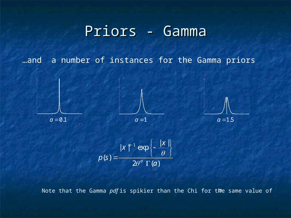
Priors - GammaPriors - Gamma

1 | || | exp

( )2 ( )

a

a

xx

p sa

0.1a 1a 1.5a

…and a number of instances for the Gamma priors

Note that the Gamma pdf is spikier than the Chi for the same value ofa

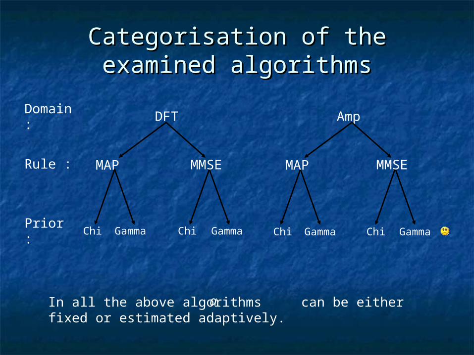
Categorisation of the examined Categorisation of the examined algorithmsalgorithms

DFT AmpDomain :

ChiPrior : Chi ChiChiGamma

Gamma

Gamma

Gamma

MMSEMAP MMSEMAPRule :

In all the above algorithms can be either fixed or estimated adaptively.

a

ResultsResults

In the following we will present results from simulations performed with the above algorithms

We will first show results for fixed prior shapes.

Finally, we will examine the case when the priors change shape adaptively.

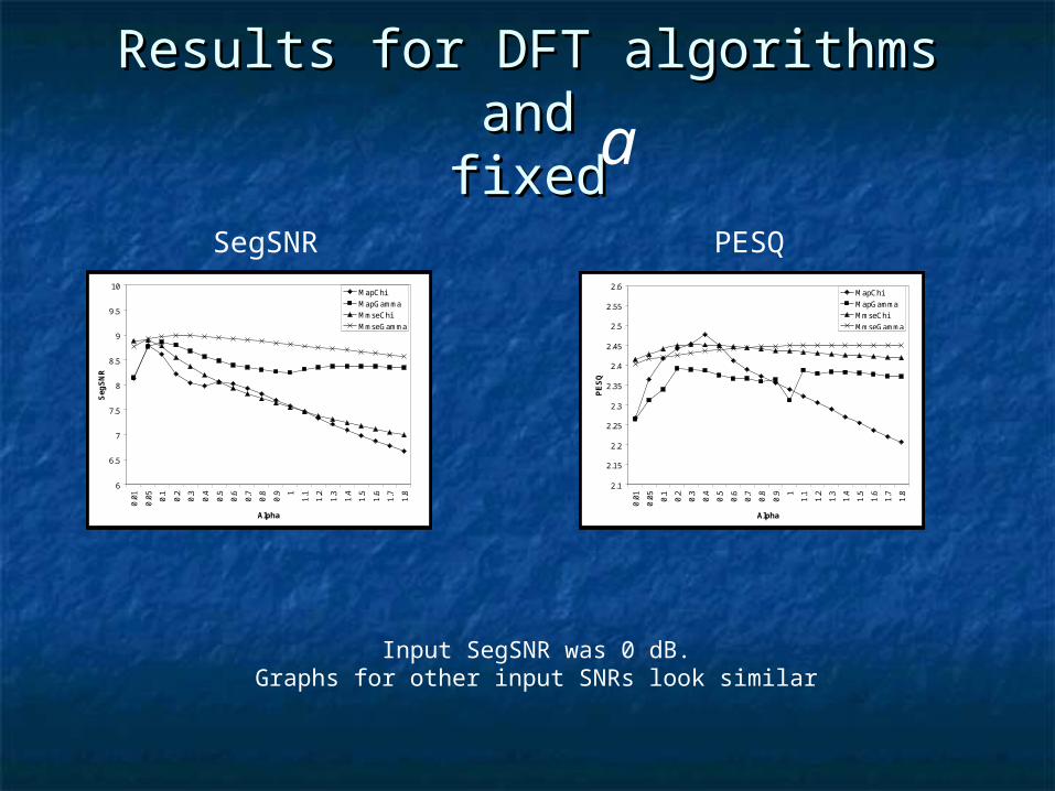
Results for DFT algorithms andResults for DFT algorithms andfixedfixed

Input SegSNR was 0 dB.Graphs for other input SNRs look similar

6

6.5

7

7.5

8

8.5

9

9.5

10

0.01

0.05 0.1

0.2

0.3

0.4

0.5

0.6

0.7

0.8

0.9 1

1.1

1.2

1.3

1.4

1.5

1.6

1.7

1.8

Alpha

SegSNR

MapChi

6

6.5

7

7.5

8

8.5

9

9.5

10

0.01

0.05 0.1

0.2

0.3

0.4

0.5

0.6

0.7

0.8

0.9 1

1.1

1.2

1.3

1.4

1.5

1.6

1.7

1.8

Alpha

SegSNR

MapChi

MmseChi

6

6.5

7

7.5

8

8.5

9

9.5

10

0.01

0.05 0.1

0.2

0.3

0.4

0.5

0.6

0.7

0.8

0.9 1

1.1

1.2

1.3

1.4

1.5

1.6

1.7

1.8

Alpha

SegSNR

MapChi

MapGamma

MmseChi

6

6.5

7

7.5

8

8.5

9

9.5

10

0.01

0.05 0.1

0.2

0.3

0.4

0.5

0.6

0.7

0.8

0.9 1

1.1

1.2

1.3

1.4

1.5

1.6

1.7

1.8

Alpha

SegSNR

MapChi

MapGamma

MmseChi

MmseGamma

2.1

2.15

2.2

2.25

2.3

2.35

2.4

2.45

2.5

2.55

2.6

0.01

0.05 0.1

0.2

0.3

0.4

0.5

0.6

0.7

0.8

0.9 1

1.1

1.2

1.3

1.4

1.5

1.6

1.7

1.8

Alpha

PESQ

MapChi

2.1

2.15

2.2

2.25

2.3

2.35

2.4

2.45

2.5

2.55

2.6

0.01

0.05 0.1

0.2

0.3

0.4

0.5

0.6

0.7

0.8

0.9 1

1.1

1.2

1.3

1.4

1.5

1.6

1.7

1.8

Alpha

PESQ

MapChi

MmseChi

2.1

2.15

2.2

2.25

2.3

2.35

2.4

2.45

2.5

2.55

2.6

0.01

0.05 0.1

0.2

0.3

0.4

0.5

0.6

0.7

0.8

0.9 1

1.1

1.2

1.3

1.4

1.5

1.6

1.7

1.8

Alpha

PESQ

MapChi

MapGamma

MmseChi

2.1

2.15

2.2

2.25

2.3

2.35

2.4

2.45

2.5

2.55

2.6

0.01

0.05 0.1

0.2

0.3

0.4

0.5

0.6

0.7

0.8

0.9 1

1.1

1.2

1.3

1.4

1.5

1.6

1.7

1.8

Alpha

PESQ

MapChi

MapGamma

MmseChi

MmseGamma

aSegSNR

PESQ

SegSNR

PESQ

6

6.5

7

7.5

8

8.5

9

9.5

10

0.01

0.05 0.1

0.2

0.3

0.4

0.5

0.6

0.7

0.8

0.9 1

1.1

1.2

1.3

1.4

1.5

1.6

1.7

1.8

Alpha

SegSNR

MapChi

6

6.5

7

7.5

8

8.5

9

9.5

10

0.01

0.05 0.1

0.2

0.3

0.4

0.5

0.6

0.7

0.8

0.9 1

1.1

1.2

1.3

1.4

1.5

1.6

1.7

1.8

Alpha

SegSNR

MapChi

MmseChi

6

6.5

7

7.5

8

8.5

9

9.5

10

0.01

0.05 0.1

0.2

0.3

0.4

0.5

0.6

0.7

0.8

0.9 1

1.1

1.2

1.3

1.4

1.5

1.6

1.7

1.8

Alpha

SegSNR

MapChi

MapGamma

MmseChi

MapChi

2.1

2.15

2.2

2.25

2.3

2.35

2.4

2.45

2.5

2.55

2.6

0.01

0.05 0.1

0.2

0.3

0.4

0.5

0.6

0.7

0.8

0.9 1

1.1

1.2

1.3

1.4

1.5

1.6

1.7

1.8

Alpha

PESQ

MapChi

2.1

2.15

2.2

2.25

2.3

2.35

2.4

2.45

2.5

2.55

2.6

0.01

0.05 0.1

0.2

0.3

0.4

0.5

0.6

0.7

0.8

0.9 1

1.1

1.2

1.3

1.4

1.5

1.6

1.7

1.8

Alpha

PESQ

MapChi

MmseChi

2.1

2.15

2.2

2.25

2.3

2.35

2.4

2.45

2.5

2.55

2.6

0.01

0.05 0.1

0.2

0.3

0.4

0.5

0.6

0.7

0.8

0.9 1

1.1

1.2

1.3

1.4

1.5

1.6

1.7

1.8

Alpha

PESQ

MapChi

MapGamma

MmseChi

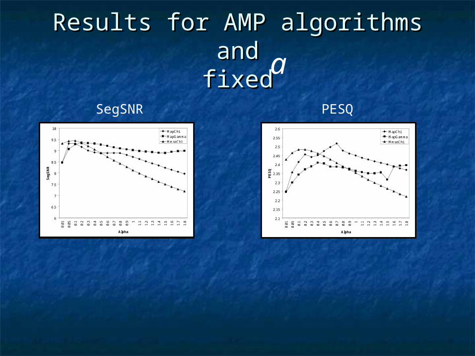
Results for AMP algorithms andResults for AMP algorithms andfixedfixeda

Audio samples and spectrogramsAudio samples and spectrograms

Time [s]F

requ

ency

[Hz]

0 0.2 0.4 0.6 0.8 1 1.2 1.4 1.6 1.80

500

1000

1500

2000

2500

3000

3500

Time [s]

Fre

quen

cy [H

z]

0 0.2 0.4 0.6 0.8 1 1.2 1.4 1.6 1.80

500

1000

1500

2000

2500

3000

3500

In the following we shall present some audio samples and spectrograms of enhanced speech with the so far examined algorithms. The clean and the noisy speech segments used in the simulations are presented below

Clean Speech Noisy Speech

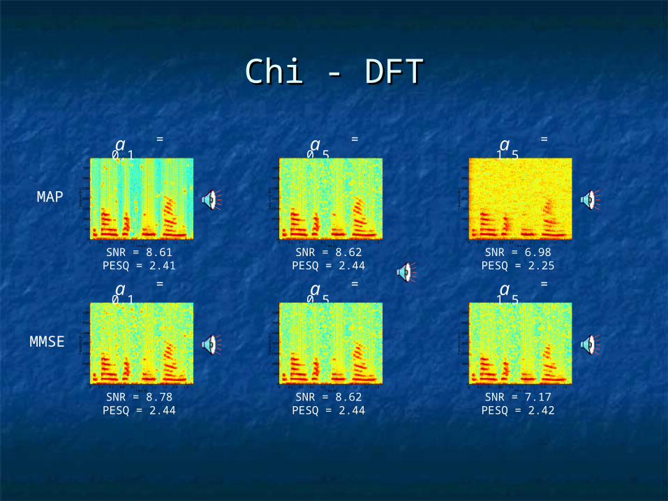
Chi - DFTChi - DFT

Time [s]

Fre

quen

cy [H

z]

0 0.2 0.4 0.6 0.8 1 1.2 1.4 1.6 1.80

500

1000

1500

2000

2500

3000

3500

Time [s]

Fre

quen

cy [H

z]

0 0.2 0.4 0.6 0.8 1 1.2 1.4 1.6 1.80

500

1000

1500

2000

2500

3000

3500

= 1.5a

= 1.5a

SNR = 7.17PESQ = 2.42

SNR = 6.98PESQ = 2.25

Time [s]

Fre

quen

cy [H

z]

0 0.2 0.4 0.6 0.8 1 1.2 1.4 1.6 1.80

500

1000

1500

2000

2500

3000

3500

Time [s]

Fre

quen

cy [H

z]

0 0.2 0.4 0.6 0.8 1 1.2 1.4 1.6 1.80

500

1000

1500

2000

2500

3000

3500

= 0.1a

= 0.1a

SNR = 8.61PESQ = 2.41

SNR = 8.78PESQ = 2.44

= 0.5a

= 0.5a

SNR = 8.62PESQ = 2.44

SNR = 8.62PESQ = 2.44

MMSE

MAP

Time [s]

Fre

quen

cy [H

z]

0 0.2 0.4 0.6 0.8 1 1.2 1.4 1.6 1.80

500

1000

1500

2000

2500

3000

3500

Time [s]

Fre

quen

cy [H

z]

0 0.2 0.4 0.6 0.8 1 1.2 1.4 1.6 1.80

500

1000

1500

2000

2500

3000

3500

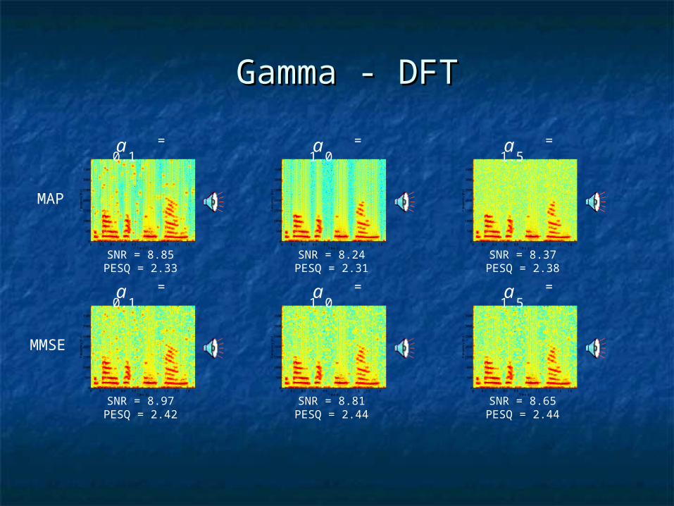
Gamma - DFTGamma - DFT

Time [s]

Fre

quen

cy [H

z]

0 0.2 0.4 0.6 0.8 1 1.2 1.4 1.6 1.80

500

1000

1500

2000

2500

3000

3500

Time [s]

Fre

quen

cy [H

z]

0 0.2 0.4 0.6 0.8 1 1.2 1.4 1.6 1.80

500

1000

1500

2000

2500

3000

3500

= 1.5a

= 1.5a

SNR = 8.65PESQ = 2.44

SNR = 8.37PESQ = 2.38

Time [s]

Fre

quen

cy [H

z]

0 0.2 0.4 0.6 0.8 1 1.2 1.4 1.6 1.80

500

1000

1500

2000

2500

3000

3500

Time [s]

Fre

quen

cy [H

z]

0 0.2 0.4 0.6 0.8 1 1.2 1.4 1.6 1.80

500

1000

1500

2000

2500

3000

3500

= 0.1a

= 0.1a

SNR = 8.85PESQ = 2.33

SNR = 8.97PESQ = 2.42

Time [s]

Fre

quen

cy [H

z]

0 0.2 0.4 0.6 0.8 1 1.2 1.4 1.6 1.80

500

1000

1500

2000

2500

3000

3500

Time [s]

Fre

quen

cy [H

z]

0 0.2 0.4 0.6 0.8 1 1.2 1.4 1.6 1.80

500

1000

1500

2000

2500

3000

3500

= 1.0a

= 1.0a

SNR = 8.24PESQ = 2.31

SNR = 8.81PESQ = 2.44

MMSE

MAP

Chi - AMPChi - AMP

Time [s]

Fre

quen

cy [H

z]

0 0.2 0.4 0.6 0.8 1 1.2 1.4 1.6 1.80

500

1000

1500

2000

2500

3000

3500

Time [s]

Fre

quen

cy [H

z]

0 0.2 0.4 0.6 0.8 1 1.2 1.4 1.6 1.80

500

1000

1500

2000

2500

3000

3500

= 0.1a

= 0.1a

SNR = 9.31PESQ = 2.41

SNR = 9.43PESQ = 2.48

Time [s]

Fre

quen

cy [H

z]

0 0.2 0.4 0.6 0.8 1 1.2 1.4 1.6 1.80

500

1000

1500

2000

2500

3000

3500

Time [s]

Fre

quen

cy [H

z]

0 0.2 0.4 0.6 0.8 1 1.2 1.4 1.6 1.80

500

1000

1500

2000

2500

3000

3500

= 0.5a

= 0.5a

SNR = 8.88PESQ = 2.47

SNR = 8.88PESQ = 2.44

Time [s]

Fre

quen

cy [H

z]

0 0.2 0.4 0.6 0.8 1 1.2 1.4 1.6 1.80

500

1000

1500

2000

2500

3000

3500

Time [s]

Fre

quen

cy [H

z]

0 0.2 0.4 0.6 0.8 1 1.2 1.4 1.6 1.80

500

1000

1500

2000

2500

3000

3500

= 1.0a

= 1.0a

SNR = 8.12PESQ = 2.35

SNR = 8.71PESQ = 2.44

MMSE

MAP

Gamma - AMPGamma - AMP

Time [s]

Fre

quen

cy [H

z]

0 0.2 0.4 0.6 0.8 1 1.2 1.4 1.6 1.80

500

1000

1500

2000

2500

3000

3500

= 0.1a

SNR = 9.28PESQ = 2.34

Time [s]

Fre

quen

cy [H

z]

0 0.2 0.4 0.6 0.8 1 1.2 1.4 1.6 1.80

500

1000

1500

2000

2500

3000

3500

= 0.5a

SNR = 9.26PESQ = 2.40

Time [s]

Fre

quen

cy [H

z]

0 0.2 0.4 0.6 0.8 1 1.2 1.4 1.6 1.80

500

1000

1500

2000

2500

3000

3500

= 1.8a

SNR = 8.99PESQ = 2.39

MAP

Results revisitedResults revisited

6

6.5

7

7.5

8

8.5

9

9.5

10

0.01

0.05 0.

1

0.2

0.3

0.4

0.5

0.6

0.7

0.8

0.9 1

1.1

1.2

1.3

1.4

1.5

1.6

1.7

1.8

Alpha

SegSNR

MapChi

MapGamma

MmseChi

MmseGamma

2.1

2.15

2.2

2.25

2.3

2.35

2.4

2.45

2.5

2.55

2.6

0.0

1

0.0

5

0.1

0.2

0.3

0.4

0.5

0.6

0.7

0.8

0.9 1

1.1

1.2

1.3

1.4

1.5

1.6

1.7

1.8

Alpha

PESQ

MapChi

MapGamma

MmseChi

MmseGamma

6

6.5

7

7.5

8

8.5

9

9.5

10

0.0

1

0.0

5

0.1

0.2

0.3

0.4

0.5

0.6

0.7

0.8

0.9 1

1.1

1.2

1.3

1.4

1.5

1.6

1.7

1.8

Alpha

SegSNR

MapChi

MapGamma

MmseChi

2.1

2.15

2.2

2.25

2.3

2.35

2.4

2.45

2.5

2.55

2.6

0.0

1

0.0

5

0.1

0.2

0.3

0.4

0.5

0.6

0.7

0.8

0.9 1

1.1

1.2

1.3

1.4

1.5

1.6

1.7

1.8

Alpha

PESQ

MapChi

MapGamma

MmseChi

MMSE algorithms reduce the background noise, especially for low SNRs

Some examples follow…

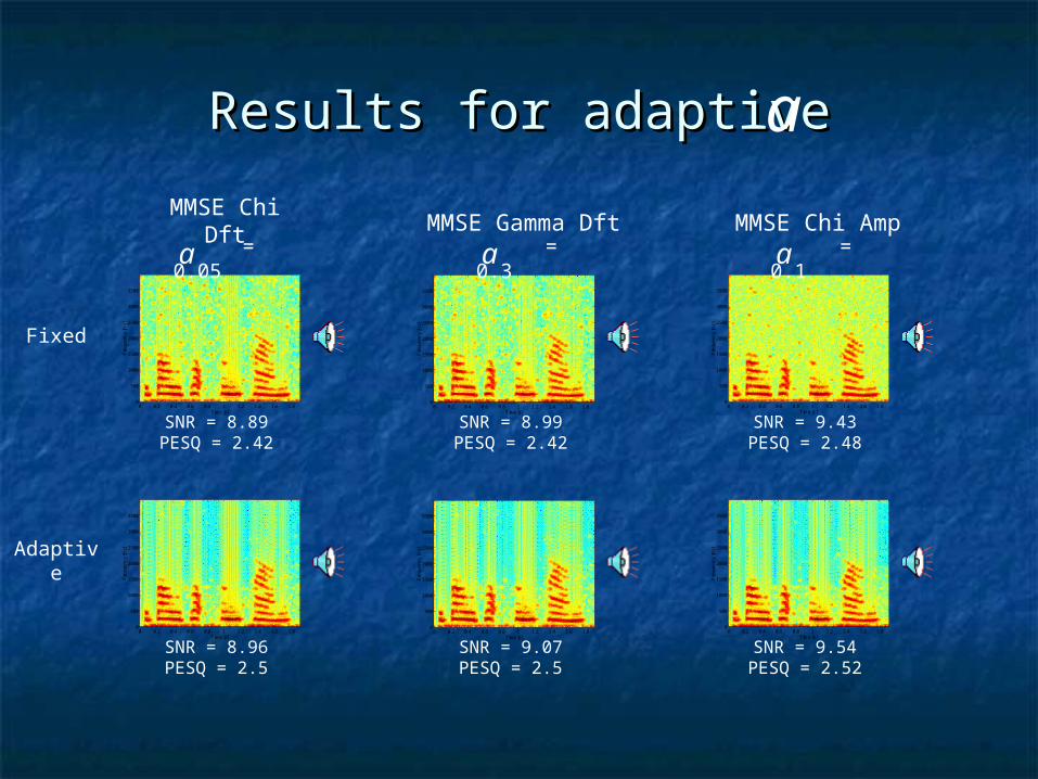
Results for adaptiveResults for adaptivea

MAP algorithms do not seem to improve their performance with adaptive values ofa

Results for adaptiveResults for adaptivea

Time [s]

Fre

quen

cy [H

z]

0 0.2 0.4 0.6 0.8 1 1.2 1.4 1.6 1.80

500

1000

1500

2000

2500

3000

3500

Time [s]

Fre

quen

cy [H

z]

0 0.2 0.4 0.6 0.8 1 1.2 1.4 1.6 1.80

500

1000

1500

2000

2500

3000

3500

Time [s]F

requ

ency

[Hz]

0 0.2 0.4 0.6 0.8 1 1.2 1.4 1.6 1.80

500

1000

1500

2000

2500

3000

3500

Time [s]

Fre

quen

cy [H

z]

0 0.2 0.4 0.6 0.8 1 1.2 1.4 1.6 1.80

500

1000

1500

2000

2500

3000

3500

Time [s]

Fre

quen

cy [H

z]

0 0.2 0.4 0.6 0.8 1 1.2 1.4 1.6 1.80

500

1000

1500

2000

2500

3000

3500

Time [s]

Fre

quen

cy [H

z]

0 0.2 0.4 0.6 0.8 1 1.2 1.4 1.6 1.80

500

1000

1500

2000

2500

3000

3500

= 0.05a

SNR = 8.89PESQ = 2.42

SNR = 8.96PESQ = 2.5

= 0.3a

SNR = 8.99PESQ = 2.42

SNR = 9.07PESQ = 2.5

= 0.1a

SNR = 9.54PESQ = 2.52

SNR = 9.43PESQ = 2.48

Fixed

Adaptive

MMSE Chi Dft MMSE Gamma Dft MMSE Chi Amp