Bayesian Methods for Mixture Modeling · Abstract This Master’s thesis is mostly focused on Bayesian methods for the selection and testing of discrete mixture models. The main problem

Valeriu Savcenco

TRITA-NA-E04001

Bayesian Methods for Mixture Modeling

NADA

Numerisk analys och datalogi Department of Numerical AnalysisKTH and Computer Science100 44 Stockholm Royal Institute of Technology

SE-100 44 Stockholm, Sweden

Valeriu Savcenco

TRITA-NA-E04001

Master’s Thesis in Computer Science (20 credits)at the Scientific Computing International Master Program,

Royal Institute of Technology year 2004Supervisor at Nada was Stefan Arnborg

Examiner was Stefan Arnborg3

Bayesian Methods for Mixture Modeling

AbstractThis Master’s thesis is mostly focused on Bayesian methods for the selection andtesting of discrete mixture models.

The main problem that is studied in the project is the analysis of data setsof several categorical variables (e.g. test items, symptoms, genes) collected on aset of subjects. We fit a discrete mixture model to the data which means thatthe dependencies among the different variables are captured by a latent categoricalvariable. We assume that the manifest variables are independent given the latentvariable. We implemented a Matlab program - an exploratory data tool that searchesfor latent classes of interest for given data sets.

Another problem studied in the project is the possibility of having missing ob-served data. For solving this problem we introduce an additional step in Gibbssampling in which the values for the missing data are sampled.

The methods described in the thesis are applied for a psychiatric diagnostics dataset and for a data set containing information from schizophrenia affected and healthypersons.

Bayesianska metoder for identifiering avsammansatta fordelningar

SammanfattningDetta examensarbete beskriver en metod for att identifiera en familj av fordelningar

ur ett sample med flera diskreta variabler. En fordelning i familjen ar en blandning(mixture) sammansatt av flera enklare fordelningar, var och en med oberoende vari-abler.

Vi bestammer en posteriorifordelning over antal komponenter och parametrarnafor varje komponent med Markov Chain Monte Carlo. Detta ger en latent variabel -klasstillhorighet - for varje individ i vart sample. Ett explorativt dataanalysverktyghar implementerats som ett Matlab-program. Metoden har utvidgats till att hanterasaknade data (data missing at random).

Metoderna tillampas genom analys av tva datamangder som erhallits fran psyki-atriforskning.

Acknowledgements

I would like to thank my supervisor Professor Stefan Arnborg for valuable

suggestions and ideas during the work.

I am very grateful for the financial support of Swedish Institute whichgranted me with the scholarship.

Contents

1 Introduction 1

1.1 Basic definitions . . . . . . . . . . . . . . . . . . . . . . . . . . . 2

1.2 Missing data formulation . . . . . . . . . . . . . . . . . . . . . . 2

1.3 Number of components . . . . . . . . . . . . . . . . . . . . . . . 3

2 Basic Markov Chain Monte Carlo techniques 5

2.1 Bayesian inference . . . . . . . . . . . . . . . . . . . . . . . . . 5

2.2 Monte Carlo Integration . . . . . . . . . . . . . . . . . . . . . . 6

2.3 Markov chains . . . . . . . . . . . . . . . . . . . . . . . . . . . . 7

2.4 The Gibbs sampler . . . . . . . . . . . . . . . . . . . . . . . . . 8

3 Bayesian analysis of mixtures with an unknown number of

components 10

3.1 The Bayes factor . . . . . . . . . . . . . . . . . . . . . . . . . . 10

3.2 Computation of the marginal likelihood . . . . . . . . . . . . . . 11

3.3 Non-identifiability of the mixture components . . . . . . . . . . 13

3.4 Treatment of missing observed data . . . . . . . . . . . . . . . . 14

4 Results 15

4.1 The psychiatric judgement data set . . . . . . . . . . . . . . . . 15

4.2 Model estimation . . . . . . . . . . . . . . . . . . . . . . . . . . 15

4.3 Model estimation in case with missing observed data . . . . . . 17

4.4 Schizophrenia related data set . . . . . . . . . . . . . . . . . . . 20

Bibliography 27

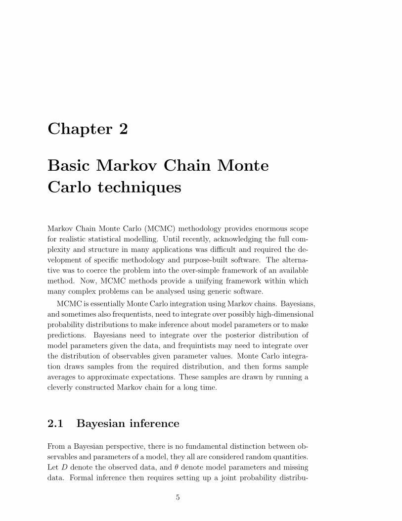
Chapter 1

Introduction

Since the first attempt to analyse a mixture model by Pearson (1894), mixture

models have been used in an incredible range of applications. Characteristic

examples come from fisheries research, sedimentology, astronomy and medical

diagnosis.

Mixture distributions are typically used to model data in which each ob-

servation is assumed to have arisen from one of a number of different classes.

They also provide a convenient and flexible family of models for probability

density estimation.

The Bayesian approach is an extremely powerful paradigm to analyse the

results of scientific experimentation. It uses a probability concept which closely

matches that used in ordinary language, directly solves the more relevant sci-

entific questions on data analysis, and may be applied to complex, richly struc-

tured problems, fairly inaccesible to traditional statistical methods.

While a Bayesian analysis of mixture models has certain advantages over

a classical approach, it is not without its problems. In theory quantities of

interest may be written down as integrals, but in practice these integrals cannot

be solved analytically, so numerical methods are required.

This project is mostly focused on Bayesian methods for the selection and

testing of discrete mixture models.

The main problem that is studied in the project is the analysis of data sets

of several categorical variables (e.g. test items, symptoms, genes) collected on

a set of subjects. We fit a discrete mixture model to the data which means

that the dependencies among the different variables are captured by a latent

categorical variable. We assume that the manifest variables are independent

conditional on this latent variable. We implemented a Matlab program - an

1

Introduction

exploratory data tool that searches for latent classes of interest for given data

sets.

Another problem that is studied in the project is the possibility of having

missing observed data. For solving this problem we introduce an additional

step in Gibbs sampling in which the values for the missing data items are

sampled.

1.1 Basic definitions

The mixture models that we consider are given by the observation of n inde-

pendent random variables x1, ..., xn, from a k-component mixture density:

f (xi) =k∑

j=1

pjfj (xi) , i = 1, ..., n, (1.1)

where

pj > 0, j = 1, ..., k; p1 + ... + pk = 1

and

fj(x) ≥ 0, j = 1, ..., k.

The parameters p1, ..., pk are called the mixing weights and f1(x), ..., fk(x)

the component densities of the mixture.

Mixture models are typically used to model data where each observation

is assumed to have arisen from one of k groups, each group being suitably

modelled by a density from the parametric family f . The mixture weights

then represent the relative frequency of occurrence of each group in the pop-

ulation, and the model provides a framework by which observations may be

clustered together into groups for discrimination or classification. For a more

comprehensive description of the mixture models see [22].

Mixture models can describe quite exotic distributions with few parameters

and a high degree of accuracy. They are satisfactory competitors to more

sophisticated methods of nonparametric estimation, in terms of both accuracy

and inferential structure.

1.2 Missing data formulation

A mixture model can always be expressed in terms of missing data. Let us

consider that each observation xi arose from a specific but unknown component

2

1.3. NUMBER OF COMPONENTS

zj of the mixture. Then the vector (z1, ..., zn) is the missing data part, since

it is not observed.

The model 1.1 can be written in terms of the missing data, with z1, ..., zn

assumed to be realisations of independent and identically distributed discrete

random variables Z1, ..., Zn with probability mass function

Pr (Zj = i) = pi, j = 1, ..., n; i = 1, ..., k.

Conditional on {Zi|i = 1, .., n}, x1, ..., xn are assumed to be independent

observations from the densities

p (xj|Zj = i) = fi(x), j = 1, ..., n.

Integrating out the missing data Z1, ..., Zn we obtain the model 1.1:

p (xj) =k∑

i=1

Pr (Zj = i) p (xj|Zj = i) =k∑

i=1

pifi(x) (1.2)

The introduction of the zi is not necessarily artificial, although the algorithm

works similarly whether it is natural or not. In some cases, the determination

of the posterior distribution of these indicator variables is of interest, to classify

the observations with respect to the components of the mixture.

1.3 Number of components

When one performs analysis of a mixture model, in many cases, the number

of components k is unknown. In applications where the components have a

physical interpretation, inference for k may be of interest in itself.

Inference for k may be seen as a specific example of the very common prob-

lem of choosing a model from a given set of competing models. Taking a

Bayesian approach to this problem has the advantage that it provides not only

a way of selecting a single best model, but also a coherent way of combining

results over different models. In the mixture model context this might include

performing density estimation by taking an appropriate average of density es-

timates obtained using different values of k. While model choice and model av-

eraging within the Bayesian framework are both theoretically straightforward,

they often provide a computational challenge, particularly when the compet-

ing models are of different dimensions. The use of Markov Chain Monte Carlo

methods to perform Bayesian analysis is now very common.

3

Introduction

Much previous work on mixture models estimation, Bayesian or otherwise,

has separated the issues of testing the number of components k from estimation

with k fixed. For the fixed-k case, a comprehensive Bayesian treatment using

Markov Chain Monte Carlo methods was presented in [8]. Early approaches

to the general case where k is unknown typically adopted a different style of

modelling, treating the problem as an example of ”Bayesian nonparametrics”,

and basing prior on the Dirichlet process.

Usually, the selection of the number of mixture components is done in two

ways. One way is to perform goodness-of-fit test and to extend the model until

a reasonable fit is obtained. Another way is to compare different models by

means of some summary characteristics. We will use the second way and as

such summary characteristic the Bayes factor will be used.

The main reasons for using the Bayes factor rather than performing goodness-

of-fit tests are that the Bayes factor is based on comparing the alternative

models by the posterior evidence in favor of each of them and that the Bayes

factor can be used for comparing non-nested models. The last reason is of big

importance in context of mixture models. If this method can be implemented

efficiently, it will give a better and more well-founded estimate of model un-

certainty than EM-methods currently used.

4

Chapter 2

Basic Markov Chain Monte

Carlo techniques

Markov Chain Monte Carlo (MCMC) methodology provides enormous scope

for realistic statistical modelling. Until recently, acknowledging the full com-

plexity and structure in many applications was difficult and required the de-

velopment of specific methodology and purpose-built software. The alterna-

tive was to coerce the problem into the over-simple framework of an available

method. Now, MCMC methods provide a unifying framework within which

many complex problems can be analysed using generic software.

MCMC is essentially Monte Carlo integration using Markov chains. Bayesians,

and sometimes also frequentists, need to integrate over possibly high-dimensional

probability distributions to make inference about model parameters or to make

predictions. Bayesians need to integrate over the posterior distribution of

model parameters given the data, and frequintists may need to integrate over

the distribution of observables given parameter values. Monte Carlo integra-

tion draws samples from the required distribution, and then forms sample

averages to approximate expectations. These samples are drawn by running a

cleverly constructed Markov chain for a long time.

2.1 Bayesian inference

From a Bayesian perspective, there is no fundamental distinction between ob-

servables and parameters of a model, they all are considered random quantities.

Let D denote the observed data, and θ denote model parameters and missing

data. Formal inference then requires setting up a joint probability distribu-

5

CHAPTER 2. BASIC MARKOV CHAIN MONTE CARLOTECHNIQUES

tion P (D, θ) over all random quantities. This joint distribution comprises two

parts: a prior distribution P (θ) and a likelihood P (D|θ). Specifying P (θ)

and P (D|θ) gives a full probability model, in which

P (D, θ) = P (D|θ) P (θ) .

Having observed D, Bayes theorem is used to determine the distribution of

θ conditional on D:

P (θ|D) =P (θ) P (D|θ)∫P (θ) P (D|θ) dθ

.

This is called the posterior distribution of θ, and is the object of all Bayesian

inference.

In general case, the posterior expectation of a function f(θ) is

E [f(θ)|D] =

∫f(θ)P (θ) P (D|θ) dθ∫

P (θ) P (D|θ) dθ. (2.1)

2.2 Monte Carlo Integration

Let X be a vector of k random variables, with distribution π(·). X will denote

model parameters and missing data, and π(·) will denote a posterior distribu-

tion. Then 2.1 can be written as:

E [f(X)] =

∫f(x)π(x)dx∫

π(x)dx(2.2)

Monte Carlo integration evaluates E [f(X)] by drawing samples {Xt, t =

1, ..., n} from π(·) and then approximating

E [f(X)] ≈ 1

n

n∑t=1

f (Xt) (2.3)

When the samples {Xt} are independent, laws of large numbers ensure that

the approximation can be made as accurate as desired by increasing the sample

size n.

In general, drawing samples {Xt} independently from π(·) is not feasible,

since π(·) can be quite non-standard. However the {Xt} need not necessarily be

independent. The {Xt} can be generated by any process which draws samples

throughout the support of π(·) in the correct proportions. One way of doing

this is through a Markov chain having π(·) as its stationary distribution. This

way of doing is called Markov Chain Monte Carlo.

6

2.3. MARKOV CHAINS

2.3 Markov chains

We present here the essential theory required in developing Monte Carlo meth-

ods based on Markov chains. The most significant result is that certain Markov

chains converge to a unique invariant distribution, and can be used to estimate

expectations with respect to this distribution.

A Markov chain is a series of random variables, X(0), X(1), X(2), ..., in which

the influence of the values of X(0), ..., X(n) on the distribution of X(n+1) is

mediated entirely by the value of X(n), More formally,

P(x(n+1)|x(n), {x(t) : t ∈ ε}

)= P

(x(n+1)|x(n)

)(2.4)

where ε is any subset of {0, ..., n − 1}. The indexes, t = 0, 1, 2, ..., are often

viewed as representing successive ”times”. The X(t) have a common range,

the state space of the Markov chain.

A Markov chain can be specified by giving the marginal distribution for X(0)

- the initial probabilities of the various states, and the conditional distributions

for X(n+1) given the possible values for X(n) - the transition probabilities for

one state to follow another state.

We will denote the initial probability of state x as p0(x), and the transition

probability for state x′ at time n+1 to follow state x at time n as Tn (x, x′). If

the transition probabilities do not depend on the time then the Markov chain

is said to be homogeneous or stationary and the transition probabilities are

written simply as T (x, x′).

Using the transition probabilities, one can find the probability of state x

occuring at time n+1, denoted by pn+1(x), from the corresponding probabilities

at time n, as follows:

pn+1(x) =∑

ex pn(x)Tn(x, x) (2.5)

Given the initial probabilities, p0, this determines the behaviour of the chain

at all times.

An invariant or stationary distribution over the states of a Markov chain

is one that persists forever once it is reached. More formally, the distribution

given by the probabilities π(x) is invariant with respect to the Markov chain

with transition probabilities Tn (x, x′) if, for all n,

π(x) =∑

ex π(x)Tn(x, x) (2.6)

A Markov chain can have more than one invariant distribution.

7

CHAPTER 2. BASIC MARKOV CHAIN MONTE CARLOTECHNIQUES

A Markov chain is said to be ergodic if the probabilities at time n, pn(x),

converge to the same invariant distribution as n →∞, regardless of the choice

of initial probabilities p0(x). An ergodic Markov chain can have only one

invariant distribution, which is also referred to as its equilibrium distribution.

Fundamental theorem. If a homogeneous Markov chain on a finite state

space with transition probabilities T (x, x′) has π as an invariant distribution

and

ν = minx

minx′:π(x′)>0

T (x, x′)/π(x′) > 0 (2.7)

then the Markov chain is ergodic, i.e., regardless of the initial probabilities,

p0(x)

limn→∞

pn(x) = π(x) (2.8)

for all x. A bound on the rate of converegence is given by

|π(x)− pn(x)| ≤ (1− ν)n (2.9)

Furthermore, if a(x) is any real-valued function of the state, then the expec-

tation of a with respect to the distribution pn, written En[a], converges to its

expectation with respect to π, written 〈a〉, with

|〈a〉 − En[a]| ≤ (1− ν)n maxx,x′

|a(x)− a(x′)| (2.10)

A proof of this theorem can be found in [14].

The theorem as stated guarantees only that at large times the distribution

will be close to the invariant distribution. It does not say how dependent

the states at different times might be, and hence does not guarantee that

the average value of a function over a long period of time converges to the

function’s expected value.

2.4 The Gibbs sampler

The Gibbs sampler is a method of constructing a Markov chain with sta-

tionary distribution p (θ|x) when Θ ∈ E can be partitioned into components

(Θ1, ..., Θr) ∈ E1 × ...× Er, of possibly differing dimensions, where we cannot

sample directly from p (θ|x) = p (θ1, ..., θr|x) but can sample directly from full

conditional distributions

p (θ1|x, θ2, ..., θr) , ..., p (θr|x, θ1, ..., θr−1) .

8

2.4. THE GIBBS SAMPLER

Gibbs sampling algorithm. Given the state Θ(t) = θ(t) at time t, the values

for Θ(t+1) can be simulated in r steps as follows:

Step 1: sample Θ(t+1)1 from p

(θ1|x, θ

(t)2 , ..., θ

(t)r

)Step 2: sample Θ

(t+1)2 from p

(θ2|x, θ

(t)1 , θ

(t)3 ..., θ

(t)r

).....

Step r: sample Θ(t+1)r from p

(θr|x, θ

(t)1 , ..., θ

(t)r−1

)The above algorithm defines a Markov chain with stationary distribution

p (θ1, ..., θr|x). This algorithm requires us to choose a starting value Θ(0).

Ideally we would sample Θ(0) from the invariant distribution p (θ|x) of the

Markov chain, but in most cases this is not possible, and so Θ(0) is tipically

chosen at random from the prior distribution for θ. In order to reduce the

dependence of the estimator 2.3 on the choice of starting point, it is standard

practice to discard the results of the first m iterations of the MCMC sampler,

for suitable chosen m. These initial m iterations are called the burn-in period.

Gelfand and Smith in [9] illustrated the power of the Gibbs sampler to ad-

dress a wide variety of statistical issues, while Smith and Roberts in [20] showed

the natural connection between the Gibbs sampler and Bayesian statistics in

obtaining posterior distributions. The Gibbs sampler can be thought of as a

stochastic analog to the EM approaches used to obtain likelihood functions

when missing data are present. In the sampler, random sampling replaces the

expectation and maximization steps.

9

Chapter 3

Bayesian analysis of mixtures

with an unknown number of

components

When analyzing mixtures, as it was mentioned in the introduction, in many

cases the number of components k is unknown.

Usually, the selection of the number of mixture components is done in two

ways. One way is to perform goodness-of-fit test and to extend the model until

a reasonable fit is obtained. Another way is to compare different models by

means of some summary characteristics. We will use the second way and as

such summary characteristic the Bayes factor will be used.

3.1 The Bayes factor

We begin with data D assumed to have arisen under one of two hypotheses

H1 and H2 according to a probability density p (D|H1) or p (D|H2). Given

a priori probabilities p(H1) and p(H2) = 1 − p(H1), the data produce a pos-

teriori probabilities p (H1|D) and p (H2|D) = 1 − p (H1|D). Since any prior

opinion gets transformed to a posterior opinion through consideration of the

data, the transformation itself represents the evidence provided by the data.

In fact, the same transformation is used to obtain the posterior probability,

regardless of the prior probability. Once we convert to the odds scale (odds

= probability/(1-probability)), the transformation takes a simple form. From

10

3.2. COMPUTATION OF THE MARGINAL LIKELIHOOD

Bayes theorem we obtain

p (Hk|D) =p (D|Hk) p(Hk)

p (D|H1) p(H1) + p (D|H2) p(H2)(k = 1, 2), (3.1)

so thatp (H1|D)

p (H2|D)=

p (D|H1)

p (D|H2)

p(H1)

p(H2), (3.2)

and the transformation is simply multimplication by

B12 =p (D|H1)

p (D|H2), (3.3)

which is the Bayes factor. Thus, in words,

posterior odds = Bayes factor× prior odds,

and the Bayes factor is the ratio of the posterior odds of H1 to its prior odds,

regarless of the value of the prior odds. When the hypotheses H1 and H2 are

equally probable a priori so that p(H1) = p(H2) = 0.5, the Bayes factor is

equal to the posterior odds in favor of H1. The two hypotheses may well not

be equally likely a priori, however.

3.2 Computation of the marginal likelihood

Suppose we have the scores of N observed subjects on J variables arranged in

an N × J matrix X. The i-th row of the X is denoted by Xi = (xi1, ..., xiJ),

where xij may take values from {1, 2, ..., Q}. As was described in the first

chapter, the unknown categorical variable that contains the class membership

labels of the subjects is denoted by z = (z1, ..., zN) where zi ∈ {1, 2, ..., K}.Conditional on membership label zi, the scores of subject i are indepen-

dent realization from multinomial distributions with parameters 1 and πj|zi=(

πj1|zi, ..., πjQ|zi

). Then the conditional likelihood of subject i is

p (Xi|π, zi) ∝J∏

j=1

Q∏q=1

πIxij=q

jq|zi(3.4)

Because the class memberships are unknown, the likelihood of Xi is a mixture

of K class-dependent densities:

p(Xi|π) =K∑

k=1

λkp (Xi|π, zi) , (3.5)

11

CHAPTER 3. BAYESIAN ANALYSIS OF MIXTURES WITHAN UNKNOWN NUMBER OF COMPONENTS

where λk is the mixing probability of class k.

Finally

p(X|π) =N∏

i=1

p(Xi|π) =N∏

i=1

K∑k=1

λkp (Xi|π, zi) , (3.6)

For the mixing probability vector λ = (λ1, ..., λK) we take a Dirichlet(α1, ..., αK)

prior and for the probabilities πj|ziwe take a Dirichlet(β1, ..., βQ) prior.

Suppose we have models M1 and M2. From the previous sections we have

that the Bayes factor is the ratio of marginal likelihoods:

B12 =p(X|M1)

p(X|M2)(3.7)

Generally, the marginal likelihood of model M can be expressed as

p(X|M) =

∫p(X|θ, M)p(θ|M)dθ (3.8)

In practice this integral cannot be solved analytically, so numerical methods

are required. Common approximation methods are effective in particular when

the posterior is unimodal, which is not the case for mixture models.

A simulation-based method that works better for multimodal posterior den-

sities was proposed by Chib in [5]. Chib’s estimator is based on the identity

p (X|M) =p (X|M, θ∗) p (θ∗|M)

p (θ∗|X, M), (3.9)

which holds for any θ∗. Here likelihood value p (X|M, θ∗) and prior probability

p (θ∗|M) can be computed directly, and the posterior probability p (θ∗|X, M)

can be estimated from the Gibbs output:

p (θ∗|X, M) =1

T

T∑t=1

p(θ∗|X, M, Z(t)

), (3.10)

where Z(t) is the t-th draw from p(Z|X).

In calculations it is convenient to use the logarithm scale for eqution 3.9

ln (p (X|M)) = ln (p (X|M, θ∗)) + ln (p (θ∗|M))− ln (p (θ∗|X, M)) (3.11)

In our case equation 3.11 is

ln (p (X|M)) = ln (p (X|M, π∗, λ∗)) + ln (p (π∗, λ∗|M))− ln (p (π∗, λ∗|X, M))

(3.12)

12

3.3. NON-IDENTIFIABILITY OF THE MIXTURECOMPONENTS

3.3 Non-identifiability of the mixture compo-

nents

The so-called label-switching problem arises when taking a Bayesian approach

to parameter estimation and clustering using mixture models. The term label-

switching was used by Redner and Walker in [19] to describe the invariance

of the likelihood under relabelling of the mixture components. In a Bayesian

context this invariance can lead to the posterior distribution of the parameters

being highly symmetric and multimodal, making it hard to summarize. In

particular the usual practice of summarizing joint posterior distribution by

marginal distributions, and estimating quantities of interest by their posterior

mean, is often inappropriate.

Naive applications of Chib’s method to mixture models will give the correct

answer provided the Gibbs sampling chain visits all labelings of the compo-

nents. This will usually occur in theory, but in practice the time required for

a Gibbs sampling chain to sample all labelings may be very long, since these

labelings correspond to modes in the posterior distribution that will often be

isolated form each other. This lack of mixing can be solved by introducing spe-

cial relabeling transitions into the Markov chain. As noted by Neal in [17], the

Chib’s estimator must be slightly modified. The posterior of a mixture model

with K components has K! modes due to permutability of the component la-

bels of which usually only a few are covered by the simulated posterior output.

The reason for this is that the Gibbs sampler method mixes well within one of

the modes but does not always mix well between the modes.

In order for the Chib’s estimator to be correct, the Markov chain {(θ(t), Z(t)

);

t = 1, ..., T} has to explore all K! modal regions that exists. In [17] Neal sug-

gested to extend the Gibbs sampling scheme with relabeling transitions. He

added that this modification works satisfactory only if the number of mixture

components is small.

The modified Chib’s estimator now becomes

p (θ∗|X,M) =1

K!T

K!∑s=1

T∑t=1

p(θ∗|X, M, Zs(t)

), (3.13)

where by {Zs(t); t = 1, ..., T} is denoted the s-th reordering (s = 1, .., K!).

13

CHAPTER 3. BAYESIAN ANALYSIS OF MIXTURES WITHAN UNKNOWN NUMBER OF COMPONENTS

3.4 Treatment of missing observed data

Another problem studied in the project is the possibility of having missing

observed data. For solving this problem we suggest to introduce an additional

step in Gibbs sampling in which the values for the missing data are sampled.

We want to find the model, which fits the observed data and for which we

have the biggest marginal likelihood. In 3.9, p (θ∗|M) is independent of X.

So in the additional step we sample the missing observed values for which we

obtain the biggest likelihood value

p(X|M, θ∗) =N∏

i=1

K∑k=1

λ∗kp (Xi|π∗, zi) (3.14)

This method is appropriate when data are missing at random. When this

is not the case, missingness should be made into an additional category for

the variable. An example of the latter is in a diagnostic test when a subject

does not give an answer to a question. An example of the former is when a

question was not asked, and the decision not to ask was not dependent on the

condition of the subject.

14

Chapter 4

Results

Using methods proposed in the previous chapters we implemented a Matlab

program - an exploratory data tool that searches for latent classes of interest

for given data sets. We applied it to a psychiatric judgement data set and

for a data set containing information from schizophrenia affected and healthy

persons.

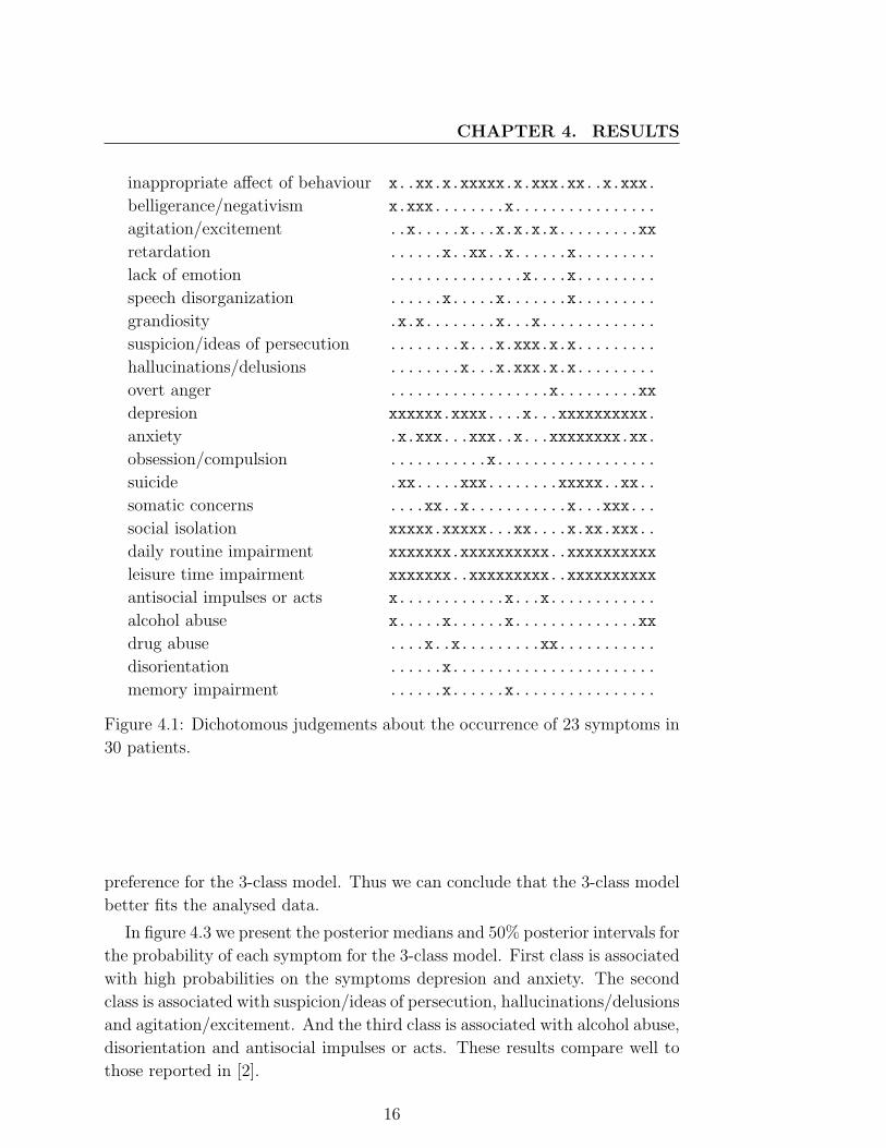
4.1 The psychiatric judgement data set

The data set used in this section is based on data described in [16] concerning

presence/absence ratings of 23 symptoms in 30 psychiatric patients. The data

consist of 0-1 judgements, made by an experienced psychiatrist about the

presence of 23 psychiatric symptoms on 30 patients. A zero was scored if the

symptom was absent, and one if it was present (see figure 4.1). In the figure

’x’ - denotes present and ’.’ - denotes absent.

4.2 Model estimation

For this data set, we estimated models with one to five classes. Regarding

posterior simulation, we simulated one Markov chain with a burn-in period of

5000 draws, and we stored the subsequent 10000 observations.

As θ∗ we took θ(t) with t = argmax(t){p(X|θ(t)

)p(θ(t)

)}.

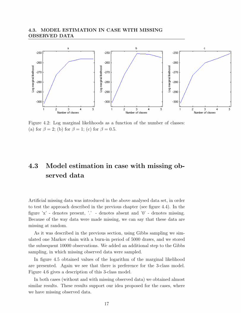
Figure 4.2 presents the values of the logarithm of the estimated marginal

likelihood p(X|M). The plots for different β show that the log marginal likeli-

hood is rather sensitive to the prior distribution. For β = 0.5 and β = 2 there

is no preference for models with small number of classes. For β = 1 there is

15

CHAPTER 4. RESULTS

inappropriate affect of behaviour x..xx.x.xxxxx.x.xxx.xx..x.xxx.

belligerance/negativism x.xxx........x................

agitation/excitement ..x.....x...x.x.x.x.........xx

retardation ......x..xx..x......x.........

lack of emotion ...............x....x.........

speech disorganization ......x.....x.......x.........

grandiosity .x.x........x...x.............

suspicion/ideas of persecution ........x...x.xxx.x.x.........

hallucinations/delusions ........x...x.xxx.x.x.........

overt anger ..................x.........xx

depresion xxxxxx.xxxx....x...xxxxxxxxxx.

anxiety .x.xxx...xxx..x...xxxxxxxx.xx.

obsession/compulsion ...........x..................

suicide .xx.....xxx........xxxxx..xx..

somatic concerns ....xx..x...........x...xxx...

social isolation xxxxx.xxxxx...xx....x.xx.xxx..

daily routine impairment xxxxxxx.xxxxxxxxxx..xxxxxxxxxx

leisure time impairment xxxxxxx..xxxxxxxxx..xxxxxxxxxx

antisocial impulses or acts x............x...x............

alcohol abuse x.....x......x..............xx

drug abuse ....x..x.........xx...........

disorientation ......x.......................

memory impairment ......x......x................

Figure 4.1: Dichotomous judgements about the occurrence of 23 symptoms in

30 patients.

preference for the 3-class model. Thus we can conclude that the 3-class model

better fits the analysed data.

In figure 4.3 we present the posterior medians and 50% posterior intervals for

the probability of each symptom for the 3-class model. First class is associated

with high probabilities on the symptoms depresion and anxiety. The second

class is associated with suspicion/ideas of persecution, hallucinations/delusions

and agitation/excitement. And the third class is associated with alcohol abuse,

disorientation and antisocial impulses or acts. These results compare well to

those reported in [2].

16

4.3. MODEL ESTIMATION IN CASE WITH MISSINGOBSERVED DATA

Figure 4.2: Log marginal likelihoods as a function of the number of classes:

(a) for β = 2; (b) for β = 1; (c) for β = 0.5.

4.3 Model estimation in case with missing ob-

served data

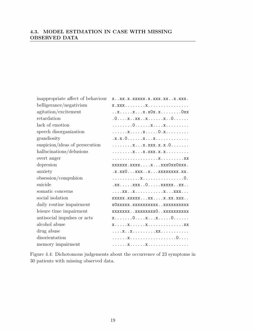
Artificial missing data was introduced in the above analysed data set, in order

to test the approach described in the previous chapter (see figure 4.4). In the

figure ’x’ - denotes present, ’.’ - denotes absent and ’0’ - denotes missing.

Because of the way data were made missing, we can say that these data are

missing at random.

As it was described in the previous section, using Gibbs sampling we sim-

ulated one Markov chain with a burn-in period of 5000 draws, and we stored

the subsequent 10000 observations. We added an additional step to the Gibbs

sampling, in which missing observed data were sampled.

In figure 4.5 obtained values of the logarithm of the marginal likelihood

are presented. Again we see that there is preference for the 3-class model.

Figure 4.6 gives a description of this 3-class model.

In both cases (without and with missing observed data) we obtained almost

similar results. These results support our idea proposed for the cases, where

we have missing observed data.

17

CHAPTER 4. RESULTS

Figure 4.3: Posterior medians and 50% posterior intervals for the probability

of each symptom being present, for each of the three classes.

18

4.3. MODEL ESTIMATION IN CASE WITH MISSINGOBSERVED DATA

inappropriate affect of behaviour x..xx.x.xxxxx.x.xxx.xx..x.xxx.

belligerance/negativism x.xxx........x................

agitation/excitement ..x.....x...x.x0x.x........0xx

retardation .0....x..xx..x......x..0......

lack of emotion ........0......x....x.........

speech disorganization ......x.....x.....0.x.........

grandiosity .x.x.0......x...x.............

suspicion/ideas of persecution ........x...x.xxx.x.x.0.......

hallucinations/delusions ........x...x.xxx.x.x.........

overt anger ..................x.........xx

depresion xxxxxx.xxxx....x...xxx0xx0xxx.

anxiety .x.xx0...xxx..x...xxxxxxxx.xx.

obsession/compulsion ...........x................0.

suicide .xx.....xxx..0.....xxxxx..xx..

somatic concerns ....xx..x...........x...xxx...

social isolation xxxxx.xxxxx...xx....x.xx.xxx..

daily routine impairment x0xxxxx.xxxxxxxxxx..xxxxxxxxxx

leisure time impairment xxxxxxx..xxxxxxxx0..xxxxxxxxxx

antisocial impulses or acts x.......0....x...x.....0......

alcohol abuse x.....x......x..............xx

drug abuse ....x..x.........xx...........

disorientation ......x..................0....

memory impairment ......x......x................

Figure 4.4: Dichotomous judgements about the occurrence of 23 symptoms in

30 patients with missing observed data.

19

CHAPTER 4. RESULTS

Figure 4.5: Log marginal likelihoods as a function of the number of

classes(missing observed data case): (a) for β = 2; (b) for β = 1; (c) for

β = 0.5.

4.4 Schizophrenia related data set

In this section we analize a data set taken from the HUBIN (HUman Brain

INformatics) project at Karolinska Institutet (see [12]). HUBIN has gathered

data on over 40 brain regions for over 300 individuals. Data also inculdes seven

cognitive performance index (CPI) test results for each individual.

The examined data consists of two important subsets. The first subset

contains volume information from the brain lobes and cerebellum. The brain

lobes include the frontal, occipital, parietal, subcortical and temporal lobes.

The frontal lobe is associated with planning, problem solving, selective atten-

tion and personality. The occipital lobe is associated with processing of visual

information. The temporal lobe is involved in perception and recognition of

auditory stimuli. The parietal lobe is associated with touch sensations such as

pressure, texture and weight. The cerebellum is a large structure that coordi-

nates and controls voluntary movements. It is divided in two lobes, connected

by the vermis. The vermis is itself divided into three structures. The vermis

is known to be involved in exploratory eye movement [18].

The second subset contains the results from cognitive ability tests and the

diagnosis. Each test measures a different aspect of cognitive ability. Rey

auditory verbal learning (RAVL) test is a series of tests of short-term memory.

Continuous perception test (CPT) measures awareness. Trail making test

(TMT) tests hand-eye coordination. Letter-number sequencing (LNS) tests

verbal working memory. Wechsler adult intelligence scale (WAIS) test is a

20

4.4. SCHIZOPHRENIA RELATED DATA SET

Figure 4.6: Posterior medians and 50% posterior intervals for the probability

of each symptom being present, for each of the three classes (missing observed

data case).

21

CHAPTER 4. RESULTS

Table 4.1: Attributes that have high values in the first class.

Attribute

CerebellarTonsil.grey

CerebellarTonsil.white

VermisLower.grey

RAVLTATOT

RAVLTB

RAVLTA6

RAVLTA7

WAIS-R

version of the classic intelligence test and it is the most comprehensive of the

tests in CPI. Wisconsin card-sorting test (WCST64) measures decision-making

ability.

We discretized the data and using the implemented program we found that

the described above data set can be classified by a 4-class model. We simulated

one Markov chain with a burn-in period of 5000 draws, and we stored the sub-

sequent 20000 observations. Almost all of the affected persons are contained in

the last two obtained classes. In figures 4.7 and 4.8 the posterior medians for

attributes for each of four classes are presented. The first class is characterized

by the high values of the attributes presented in table 4.1. Second class is char-

acterized by the high values of the attributes from table 4.2. Third class has

high values for TMTA and low values for the attributes presented in table 4.3.

Fourth class high values for Putamen.grey and low values for attributes from

table 4.4.

This classification shows us a way of how the schizophrenia affected persons

can be characterized. If a patient matches the characteristics of one of the four

obtained classes then one can conjecture the diagnosis.

22

4.4. SCHIZOPHRENIA RELATED DATA SET

Figure 4.7: Posterior medians for attributes from first subset

Figure 4.8: Posterior medians for attributes from second subset

23

CHAPTER 4. RESULTS

Table 4.2: Attributes that have high values in the second class.

Attribute

Caudate.white

Hippocampus.grey

Hippocampus.white

Cerebellum.grey

Cerebellum.white

VermisUpper.grey

VermisLower.white

Total.intracranial

Frontal.grey

Frontal.white

Occipital.grey

Occipital.white

Parietal.grey

Parietal.white

Subcortical.grey

Subcortical.white

Temporal.grey

Temporal.white

Table 4.3: Attributes that have low values in the third class.

Attribute

Cerebellum.white

VermisMiddle.white

Fontal.white

Occipital.white

Parietal.White

Subcortical.grey

Subcortical.white

Temporal.grey

Temporal.white

24

4.4. SCHIZOPHRENIA RELATED DATA SET

Table 4.4: Attributes that have low values in the fourth class.

Attribute

RAVLATOT

RAVLTB

RAVLTA7

CPT

LNS

25

Bibliography

[1] S. Arnborg, I. Agartz, H. Hall, E. Jonsson, A. Sillen and G. Sedvall (2002).

Data Mining in Schizophrenia Research - preliminary analysis. Principles

of Data Mining and Knowledge Discovery, 27-38

[2] J. Berkhof, I. Van Mechelen and A. Gelman (2003). A Bayesian approach

to the selection and testing of mixture models, Statistica Sinica, 13, 423-

442

[3] B.P. Carlin and T.A. Louis (1996). Bayes and Empirical Bayes Methods

for Data Analysis, Chapman & Hall

[4] G. Celeux, M. Hurn and C.P. Robert (2000). Computational and inferen-

tial difficulties with mixture posterior distributions, Journal of the Amer-

ican Statistical Association, 95, 957-970

[5] S. Chib (1995). Marginal likelihood from the Gibbs output, Journal of the

American Statistical Association, 90, 1313-1321

[6] S. Chib and I. Jeliazkov (2001). Marginal likelihood from the Metropolis-

Hastings output, Journal of the American Statistical Association, 96, 270-

281

[7] T.J. DiCiccio, R.E. Kass, A. Raftery and L. Wasserman (1997). Comput-

ing Bayes factors by combining simulation and asymptotic approxima-

tions, Journal of the American Statistical Association, 92, 903-915

[8] J. Diebolt and C.P. Robert (1994). Estimation of finite mixture distribu-

tions through Bayesian sampling, Journal of the Royal Statistical Society,

series B, 56, 363-375

[9] A.E. Gelfand and A.F.M. Smith (1990). Sampling-based approaches to

calculating marginal densities, Journal of the American Statistical Asso-

ciation, 85, 398-409

26

BIBLIOGRAPHY

[10] A. Gelman and T.E. Raghunathan (2001). Using conditional distributions

for missing-data imputations, Statistical Science, 3, 268–269.

[11] W.R. Gilks, S. Richardson and D.J. Spiegelhalter (1996). Markov Chain

Monte Carlo in Practice, Chapman & Hall

[12] HUBIN web site http://hubin.org

[13] R.E. Kass and A.E. Raftery (1995). Bayes factors, Journal of the Ameri-

can Statistical Association, 90, 773-795

[14] J.G. Kemeny and J.L. Snell (1960). Finite Markov chains, New York:

Springer-Verlag

[15] G. Lawyer (2003). Bayesian variable selection in schizophrenia research,

Master’s thesis

[16] I. Van Mechelen and P. De Boeck (1989). Implicit taxonomy in psychiatric

diagnosis: A case study. Journal of Social and Clinical Psychology, 8, 276-

287

[17] R. Neal (1998). Erroneous results in ”Marginal likelihood from the

Gibbs output”. Manuscript. ftp://ftp.cs.utoronto.ca/pub/radford/chib-

letter.pdf

[18] V.S. Ramachandran and S. Blakeslee (1998). Phantoms in the brain,

Fourth Estate.

[19] R.A. Redner and H.F. Walker (1984). Mixture densities, maximum likeli-

hood and the EM algorithm, SIAM Review, 26, 195-239

[20] A.F.M. Smith and G.O. Roberts (1993). Bayesian computation via the

Gibbs sampler and related Markov chain Monte-Carlo methods, Journal

of the Royal Statistical Society, series B, 55, 3-23

[21] M. Stephens (1997). Bayesian methods for mixtures of normal distribu-

tions, PhD thesis

[22] D.M. Titterington, A.F.M. Smith and U.E. Makov (1985). Statistical anal-

ysis of finite mixture distributions, John Wiley & Sons

27