Bayesian inference in incomplete multi-way tables

Bayesian inference in incomplete multi-way tables

Adrian Dobra∗, Claudia Tebaldi†& Mike West∗

[email protected] [email protected] [email protected]

February 2003

∗Institute of Statistics and Decision Sciences, Duke University, Durham, NC 27708-0251, USA.†National Center for Atmospheric Research, Boulder, CO 80305, USA.

1

Summary

We describe and illustrate approaches to Bayesian inference in multi-way contingency ta-bles for which partial information, in the form of subsets of marginal totals, is available.In such problems, interest lies in questions of inference about the parameters of modelsunderlying the table together with imputation for the individual cell entries. We discussquestions of structure related to the implications for inference on cell counts arising fromassumptions about log-linear model forms, and a class of simple and useful prior distribu-tions on the parameters of log-linear models. We then discuss “local move” and “globalmove” Metropolis-Hastings simulation methods for exploring the posterior distributions forparameters and cell counts, focusing particularly on higher-dimensional problems. As a by-product, we note potential uses of the “global move” approach for inference about numbersof tables consistent with a prescribed subset of marginal counts. Illustration and compar-ison of MCMC approaches is given, and we conclude with discussion of areas for furtherdevelopments and current open issues.

Some key words: Bayesian inference; Disclosure limitation; Fixed margins problem; Imputation; Log-linear models; Markov basis; Markov chain Monte Carlo; Missing data.

2

1 Introduction

The general problem of inference in contingency tables based on partial information in terms of observedcounts on a set of margins has become of increasing interest in recent years. We address this problemhere in a framework involving inference on parameters of statistical models underlying multi-way tablestogether with inference about missing cell entries.

Some of our initial motivating interest in this area came from socio-economic and demographicstudies that involve and rely on survey and census data representing differing levels of aggregation(hence marginalisation) of population characteristics. Much of the activity in these latter areas hasbeen referred to as micro-simulation, and the development of micro-simulation methods in areas suchas transportation policy and planning rely heavily on an ability to impute individual household levelcounts, for example, from more highly aggregated data from local or population census data.

More recently, the last several years has seen a very significant upsurge of interest in developmentof methods to aid in the creation, dissemination and use of public data sets from governmental sources,related to serious societal and legal concerns about data confidentiality and security. A range of issuesthen arise about the potential to infer individual level data from sets of interlinked aggregate-level data,and this can be focused on the problem of inferring cell counts in multi-way tables based on observationof some sets of marginal totals. Here there are questions of the extent to which sets of observed marginscan inform on cell counts under varying assumptions about the structure of candidate statistical models(such as log-linear models) (Dobra, 2002; Dobra et al., 2003), with related questions about the role andimpact of specific prior distributions on parameters of such models.

Historically, strong interest in the general problem area has focused on problems of counting tableswith prescribed marginal totals, a goal of interest in both data confidentiality studies and in the tradi-tional context of estimating significance levels in testing approaches (Agresti, 1992; Diaconis & Efron,1985; Smith et al., 1996).

Bayesian inference in this context is in principle straightforward: we aim to compute posteriordistributions for the unobserved cell counts and parameters underlying models for cell probabilities,jointly. In practice this may be addressed using Markov chain Monte Carlo (MCMC) simulations; thisrequires creativity in dealing, in particular, with simulations of the missing cell counts from appropriateconditional posterior distributions. The contributions of this article address a number of questions andneeds in support of the practical development of such methods. First, we describe the general problemand context, and develop some theoretical insights into the nature and role of assumptions about modelstructure in its relation to the problem of inference on individual cell counts based on observationof sets of marginal totals. Then, we discuss MCMC approaches to joint analysis of parameters andmissing cell counts. This uses a simple but flexible class of prior distributions on parameters of log-linear models at the parametric level. In imputing cell counts, we discuss, implement and evaluate“local move” algorithms that rely on Markov basis construction, together with a new class of “globalmove” approaches that have some relative attractions, especially as problems increase in dimensionand complexity. A detailed discussion of an example demonstrates both the implementation and theefficacy of the approaches, and we conclude with some discussion of current open issues and challenges.In addition to innovations in modelling and computation, the work represents a broad overview of therecent and current issues in this important field.

3

2 Analysis Framework and Goals

2.1 Definitions and Notation

Consider a k-way contingency table of counts over a k−vector of discrete random variables X ={X1, X2, . . . , Xk}. LetK = {1, 2, . . . , k}, and for each j ∈ K, supposeXj takes values in Ij = {1, . . . , Ij}.Write I = I1 × . . . × Ik and denote an element of I by i = (i1, . . . , ik).

The contingency table n = {n(i)}i∈I is a k-dimensional array of non-negative integer numbers, withcell entries n(i) = #{X = i}, (i ∈ I), and a total of m = I1 · . . . · Ik cells. Any set of marginal counts isobtained by summation over one or more of the X variables. For any target subset of variables D ⊂ K,the D-marginal nD of n has cells iD ∈ ID = ×j∈D Ij, with cell entries

nD(iD) =∑

j∈IK\D

n(iD, j).

If D = ∅ then n∅ is the grand total over n.Cells are ordered lexiographically with the index of the k-th variable varying fastest, so that I =

{i1, . . . , im} where i1 = (1, . . . , 1) is the first cell and im = (I1, . . . , Ik) is the last cell.

2.2 Tables with Sets of Fixed Margins

Our interest lies in problems in which we observe only subsets of margins from the full table. Supposethe l margins D = {n1, . . . , nl} are recorded. Additional information may be available, such as upperand lower bounds for some (or all) the cells in the full table, or cases of structural zeroes (that can alsobe represented by fixed upper and lower bounds, in this case each at zero). In such cases, the constraintscan be added to D without changing the development below.

Observing the margins D induces constraints that imply upper and lower bounds U(i) = max{n(i) :n ∈ T } and L(i) = min{n(i) : n ∈ T } on each cell entry n(i), i ∈ I. This limits attention to tablessatisfying these constraints. Denote the set of such tables by T – thus T is the set of k−way tablesn = {n(i)}i∈I strictly compatible with D. Write M(T ) for the number of such tables.

2.3 Statistical Models over Tables and Observed Margins

Focus on the independent Poisson sampling model that underlies the canonical multinomial distributionfor n. That is, cell counts are conditionally independent Poisson, n(i) ∼ Po(λ(i)), for each i ∈ I, withpositive means λ = {λ(i)}.

The implied probability of the observed set of margins D is then, theoretically, simply

pr(D|λ) =∑

n′∈T

pr(n′|λ). (1)

In problems of inference on λ, this defines the likelihood function, but, evidently, in other thantrivial, low-dimensional problems, direct evaluation is impossible. The essential role of n as (in part)missing or latent data underlies simulation-based methods using MCMC approaches that, followingTebaldi & West (1998a,b), iteratively resimulate the “missing” components of n and the parameters λfrom relevant conditional distributions. For the former, note that

pr(n,D|λ) =

{

pr(n|λ), if n ∈ T ,0, otherwise.

(2)

4

Then, conditional on the observed margins and model parameters, inference on the missing componentsof the table are derived directly from the implied conditional posterior

pr(n|D, λ) = pr(n|λ)/∑

n′∈T

pr(n′|λ) (3)

if n ∈ T , being zero otherwise. When embedded in a simulation-based analysis, a key technical issueis that of developing methods to simulate this distribution – proportional to the product of Poissoncomponents conditioned by the complicated set of constraints n(i) ∈ [L(i), L(i) + 1, . . . , U(i) − 1, U(i)]over cells i ∈ I defined by the observed margins D.

2.4 Population Models and Parameters

Inference about the underlying population structure is based on choices of model, such as traditionallog-linear models, for λ. Any model A has parameters θ that define λ = λ(θ). Then priors are specifiedon θ, so on λ indirectly and the latter will incorporate deterministic constraints imposed by the model.Thus we work interchangeably between λ and θ in notation. Sampling distributions are conditional onλ, thus implicitly θ. For the given model A, denote a prior density for the implied model parameters θby pr(θ|A). Posterior inference is theoretically defined through the intractable likelihood function (1).When elaborated to include the missing data to fill out the full table, the more tractable conditionalposterior is simply the prior modified by the product of Poisson likelihood components pr(n|λ).

2.5 MCMC Framework

From the above components of the posterior distribution, we may implement MCMC methods to gener-ate, ultimately, samples from pr(n, θ|D,A) by iteratively re-simulating values of θ (and hence, by directevaluation, λ), and the missing cell counts in n. Start with n(0) ∈ T . At the sth step of the algorithm,do:

• Simulate θ(s+1) from pr(θ|A, n(s)) ∝ pr(θ|A)pr(n(s)|λ(θ)), and compute the implied new value ofλ(s+1) = λ(θ(s+1)).

• Simulate n(s+1) from pr(n|D, λ(s+1)).

Section 3 discusses aspects of prior specification and model structure in their impact on pr(n|D, λ).Section 4 then considers specific priors and the resulting analysis in log-linear models. Section 5 discussesalgorithms to sampling the critical conditional posterior for the missing elements of n under the relevantdistribution (3).

3 Log-linear Models and Structural Information

Some initial theoretical results describe structural aspects of the conditional posterior pr(n|D, λ) relevantin consideration of classes of log-linear models. We first note that the conditional distribution (3) ofcourse has precisely the same form if we assume multinomial sampling for n.

First, consider the model A0 with unrelated, free parameters λ(i). Evidently, pr(n|D, λ) then dependson all the λ(i) and does not further simplify. Hence a prior specification across all the Poisson meanshas an influence in defining resulting inferences on the full table based on any set of observed marginsD.

5

Now, suppose A is a specified log-linear model defining λ in terms of underlying log-linear parametersθ. This may be defined in terms of a specification of the minimal sufficient statistics of A; supposethese to be defined by the index sets {C1, C2, . . . , Cq}, where Cj ⊂ K. Writing C = {C : ∅ 6= C ⊂Cj for some j ∈ {1, 2, . . . , q}}, the log-linear model has the form

λ(i) = µ∏

C∈C

ψC(iC), (4)

where ψC depends on i ∈ I only through the indices in C. To make the parameters identifiable, thealiasing constraints are to set each ψC(iC) = 1 whenever there exists p ∈ C with ip = 1 – see, forexample, Whittaker (1990). One immediate consequence of these aliasing constraints is that λ(i1) = µ.The parameter set is then

θ = {µ} ∪ {ψC(iC) : C ∈ C, iC ∈ IC with ip 6= 1 for p ∈ C}. (5)

The following theorem now shows that the posterior pr(n|D, λ) from (3) simplifies and does not dependon all the parameters θ from (5). This represents an extension of an earlier result by Haberman (1974).

Theorem 1. If the marginal nC of the full table is determined from D, then, under model A, the

posterior distribution pr(n|D, λ) does not depend on the parameters ψC(iC) for all iC ∈ IC.

Proof. It is not hard to see that, for any table n′, we have

∏

i∈I

λ(i)n′(i) = µn′∅

∏

C∈C

∏

iC∈IC

ψC(iC)n′C

(iC).

If n′ ∈ T , it follows that the grand totals of n′ and n are equal, i.e., n′∅ = n∅. Moreover, if the marginal

nC is known from D, then the marginals n′C and nC coincide. Thus

∏

iC∈IC

ψC(iC)n′C

(iC) =∏

iC∈IC

ψC(iC)nC(iC),

for every table n′ ∈ T . It follows that the terms involving ψC(iC), iC ∈ IC , cancel in the denominatorand the numerator of (3) and hence pr(n|D, λ) does not depend on these parameters. Note that thisposterior also does not depend on the grand mean parameter µ.

Theorem 1 implies that the model of independence A0 and the saturated log-linear model inducedifferent posterior distributions for n ∈ T since the posterior associated with the latter model depends onfewer parameters. This is somewhat surprising since these two models are usually considered equivalentsince the saturated log-linear model is just a re-parameterization of A0. Theorem 1 also shows how theform of an assumed log-linear model influences the conditional inference on n given D. We explore thisfurther.

If E is a set of subsets of K, let P(E) be those elements of E that are maximal with respect toinclusion, i.e., P(E) = {C : C ∈ E and there is no C ′ ∈ E \ {C} with C ⊂ C ′}. Write E(D) = {C :C ⊆ K and nC is known from D} and E ′(D) = {C : C ⊆ K and C /∈ E(D)}. For any model A, for thefollowing we make explicit the dependence of the Poisson means on the model, via the notation λA.

Theorem 2. Consider the family Q(D) of all the log-linear models A with minimal sufficient statistics

induced by the index sets P(E(D) ∪ E ′), where E ′ is a subset of E ′(D). For any log-linear model A′,

there exists a model A ∈ Q(D) such that pr(n|D, λA′) and pr(n|D, λA) depend on the same subset of

parameters.

6

Proof. An arbitrary log-linear model A′ has minimal sufficient statistics induced by some index setsP(E0 ∪ E′

0), where E0 ⊂ E(D) and E ′0 ⊂ E ′(D). Take the model A ∈ Q(D) defined by the index sets

P(E(D) ∪ E ′0). From Theorem 1 we see that pr(n|D, λA′) and pr(n|D, λA) depend on the same subset

of parameters.

Finally, we note the key case of the hypergeometric distribution for n given D implied by lackof dependence on parameters. This is based on the set B(D) of log-linear models A having minimalsufficient statistics P(E) for some E ⊂ E(D), i.e., cases in which the log-linear models have marginalsembedded in D. From Theorem 1 we see that, if A ∈ B(D), then the posterior pr(n|D,A, λ) is constantas a function of λ and it reduces to the hypergeometric distribution,

pr(n|D, λ) ≡ pr(n|D) =

[

∏

i∈I

n(i)!

]−1

/∑

n′∈T

[

∏

i∈I

n′(i)!

]−1

(6)

Therefore the hypergeometric distribution is a special case of the posterior in (3) obtained by condi-tioning on a log-linear model whose minimal sufficient statistics are fully determined by the availabledata D. As an aside, we note that Sundberg (1975) shows that the normalizing constant in (6) canbe directly evaluated if the log-linear model A is decomposable (Whittaker, 1990; Lauritzen, 1996);otherwise, this normalizing constant can be computed only if the set of tables T can be exhaustivelyenumerated.

4 Prior Specification and Posterior Sampling of Model Parameters

We consider classes of priors for the unknown Poisson rates λ that are consistent with the modelsdiscussed in Section 3. We start with the model of independence, A0, under which pr(λ|D, n) ≡pr(λ|n) =

∏

i pr(λ(i))|n(i)) where, for specified, independent priors, the λ(i) have independent posteriorsvia the update through independent Poisson-based likelihoods. Gamma priors are of course conjugate.

Now consider a general log-linear model A with minimal sufficient statistics {C1, C2, . . . , Cq}. Thus,if λ = {λ(i)}i∈I is consistent with A, then λ(i) is represented as in (4). As for the model of independenceA0, a relatively unstructured class of priors λ is induced by exchangeable/independence assumptionsfor the core parameters ψ(·) in this representation. As developed in West (1997), and then extendedin Tebaldi & West (1998a) and Tebaldi & West (1998b), independent gamma priors on the multiplica-tive parameters in the log-linear model representation imply that all complete, univariate conditionalposteriors are also of gamma form. Thus drawing new values for the model parameters, and hence thevalues of the λ(i), is immediately accessible using Gibbs sampling. Specifically, we note that:

• pr(µ|A, n, θ \ µ) ∝ pr(µ)µn∅ exp

{

−µ∑

i∈I

∏

C∈CψC(iC)

}

.

• for each α := ψC0(i0C0

) ∈ Θ \ µ, the complete conditional posterior for α is proportional to

pr(α)αnC0

(i0C0

)exp

−αµ∑

{i∈I:iC0=i0

C0}

∏

C∈C

ψC(iC)

. (7)

7

Now, when A is the saturated log-linear model, A is specified by one minimal sufficient statistic givenby the complete index set K. In this case C is comprises all the non-empty subsets of K. For i ∈ I theconditional posterior for β := ψK(i) is then proportional to

pr(β)βn(i) exp

−βµ∏

{C:C⊂K, C 6=K}

ψC(iC)

.

Hence, as noted, adopting independent gamma priors for each of the parameters in θ induces gammacomplete conditionals in each case. Alternatively, finite uniform priors, U(0, L) for an appropriatelylarge upper bound L, serve as at least initial objective priors. Thus, conditional on a complete table n,we can simulate new parameter values for Poisson rates λ(i), i ∈ I, via sets of independent draws fromgamma distributions, or truncated gamma distributions.

5 Imputing Cell Counts

The major component of MCMC analyses relates to the sampling algorithms to generate completetables of counts n that are consistent with the constraints defined by the marginal count information D.Direct sampling is computationally infeasible because the normalizing constant in (3) would have to beevaluated at each iteration, and this evaluation cannot be done quickly, if at all, due to the existence ofa huge number of tables consistent with D. Hence, some form of embedded Metropolis-Hastings methodis required within the overall MCMC that also samples λ.

Given a current state (n(s), λ(s+1)), a candidate table n∗ is generated from a specified proposaldistribution q(n(s), n∗), and accepted with probability

min

[

1,pr(n∗|λ(s+1))q(n∗, n(s))

pr(n(s)|λ(s+1))q(n(s), n∗)

]

. (8)

The only requirement the proposal distribution has to satisfy is that q(n(s), n∗) > 0 if and only ifq(n∗, n(s)) > 0. In contrast with the direct sampling approaches, it is neither necessary to identifythe support T of pr(n|D, λ), nor to evaluate pr(n|λ) completely across the support. If a proposaldistribution generates candidate tables outside T , they will be rejected as they lead to zero acceptanceprobabilities.

Two approaches are considered: “local” and “global” moves methods.

5.1 Local Moves

Diaconis & Sturmfels (1998) proposed generating a candidate table n∗ ∈ T using Markov bases of“local moves”. A local move g = {g(i)}i∈I is a multi-way array containing integer entries g(i) ∈{. . . ,−2,−1, 0, 1, 2, . . .}. A Markov basis MB(T ) associated with T allows any two tables n1, n2 in Tto be connected by a series of local moves g1, g2, . . . , gr, i.e.

n1 − n2 =

r∑

j=1

gj .

If the chain is currently at n(s) ∈ T , a new candidate n∗ is generated by uniformly choosing a moveg ∈ MB(T ). The candidate n∗ = n(s) + g belongs to T if and only if n∗(i) ≥ 0 for all i ∈ I. Such a

8

move g is said to be permissible for the current table n(s). If the selected move is not permissible, thechain stays at n(s). Otherwise, the chain moves to n(s+1) = n∗ with probability min{1, ρ}, where

ρ :=pr(n∗|λ(s+1))

pr(n(s)|λ(s+1))=

∏

{i∈I:n∗(i)6=n(s)(i)}

n(s)(i)!

n∗(i)!exp {g(i) log λ(s+1)(i)}.

Note that the proposal distribution q(·, ·) induced by a Markov basis is symmetric, i.e., q(n∗, n(s)) =q(n(s), n∗).

The Markov basis required by the “local move” algorithm constitutes both the strength and theweakness of this sampling procedure. The basis has to be generated before the actual simulationbegins. This extra step is likely to involve long and tedious computations in algebra systems (such asMacaulay or Cocoa) following the approach for computing a Markov basis suggested by Diaconis &Sturmfels (1998). They showed that a Markov basis for a set of tables T can be determined from aGrobner basis of a well-specified polynomial ideal.

An alternative to this algebraic approach was proposed by Dobra (2002), who gave direct formulæ fordynamically generating a Markov basis in the special case when the information D available about theoriginal table n consists of a set of marginals that define a decomposable log-linear model. Althoughthe use of Dobra’s formulæ require minimal computational effort, they cannot be extended to moregeneral cases (non-decomposable models). Nevertheless, once a Markov basis is computed, the “localmove” method can be very fast since generating a new candidate table is done only by additions andsubtractions.

Another possible disadvantage of the “local move” method is that the current table and the candidatetable can be very similar, and this is critical if T is large. The Markov bases associated with such largespaces of tables contain moves that change only few table entries and the change can be as small as ±1.For example, in the case of two-way tables with fixed row and column totals, the moves have countsof zero everywhere except four cells that contain two counts of 1 and two counts of −1. This type ofmoves are called primitive. Actually, Dobra (2002) proved that primitive moves are the only movesneeded to connect tables in the decomposable case mentioned above. Clearly, changing only four cellsin a high-dimensional contingency table that might contain millions of cells will undoubtedly lead tohigh dependencies between consecutive sample tables and the corresponding parameter values.

Therefore, with the “local move” method, one cannot control how far the chain “jumps” in the spaceof feasible tables because the jumps are pre-specified by the Markov basis employed. We present analternative to the “local move” method, which we call the “global move” method, that allows one tocontrol and adjust the distance between the current and candidate tables.

5.2 Global Moves

The idea behind the “global move” method is straightforward, and utilizes compositional sampling: anew table in T can be generated by sequentially drawing a value for each cell in the table from the setof possible values for that cell while updating the corresponding upper and lower bounds for the restof the cells. This strategy is similar to the approach and algorithm of Tebaldi & West (1998a,b) thatwas modified to a sequential form as utilized by Liu (2001) and Chen (2001). Moreover, the same ideaconstitutes the core of the generalized shuttle algorithm (Dobra, 2002) that calculates sharp upper andlower bounds for cells in a contingency tables only by efficiently exploiting the unique structure of thecategorical data.

Using the chain rule, we re-write the target distribution pr(n|D, λ) ∝ pr(n|λ) from (3) as

9

pr(n|λ) = pr(n(i1), . . . , n(im)|λ),

= pr(n(i1)|λ)m∏

a=2

pr(n(ia)|n(i1), . . . , n(ia−1), λ). (9)

The support of pr(n(i1)|λ) is a subset of the set of integers H1 defined by the upper and lower boundsinduced by D on the cell i1, i.e., H1 := {L(i1), L(i1) + 1, . . . , U(i1) − 1, U(i1)}. Similarly, the sup-port of pr(n(ia)|n(i1), . . . , n(ia−1), λ) is a subset of the set of integers Ha defined by the upper andlower bounds induced on the cell ia by D and by the additional constraints resulted from fixing thecounts in the cells i1, . . . , ia−1, i.e., Ha := {L(n; ia), L(n; ia) + 1, . . . , U(n; ia) − 1, U(n; ia)}, whereL(n; ia) = min{n′(ia) : n′ ∈ T , n′(i1) = n(i1), . . . , n′(ia−1) = n(ia−1))} and U(n; ia) = max{n′(ia) :n′ ∈ T , n′(i1) = n(i1), . . . , n′(ia−1) = n(ia−1)}.

If a Markov basis associated with the set of feasible tables T can be constructed such that this basiscontains only primitive moves, then the supports of pr(n(i1)|λ) and pr(n(ia)|n(i1), . . . , n(ia−1), λ) willbe exactly H1 and Ha, respectively. Otherwise, to the best of our knowledge, there is no theoreticalresult which shows that the supports of these two distributions should coincide with H1 and Ha, nordo we know of an example when this property does not hold.

A candidate table n∗ ∈ T is generated with the “global move” method as follows:

• Draw a value n∗(i1) from H1.

• for a = 2, . . . ,m do

1. Calculate L(n∗; ia) and U(n∗; ia).

2. Draw a value n∗(ia) from Ha.

end for

We still need a way to draw cell values from H1,H2, . . . ,Hm such that the resulting candidate tablesn∗ will be neither “too different” nor “too similar” to the current state n(s) ∈ T . Candidate tablesthat are “too different” are very likely to be rejected by the Metropolis-Hastings step, while candidatesthat are “too similar” will be likely to be accepted, but the chain will not advance fast enough in thetarget space, so inducing very correlated sample path. One approach to balancing these issues uses anannealing idea.

Consider the scaling factors v1, v2, . . . , vm with va ∈ (0, 1). For each a ∈ {1, 2, . . . ,m}, draw a valuen∗(ia) from the proposal distribution with probabilities

qa(n(s)(ia), n∗(ia)) ∝ v|n

∗(ia)−n(s)(ia)|a , (10)

Note that the current value n(s)(ia) of cell ia does not have to belong to the support Ha of qa(n(s)(ia), ·).

However, candidate cell values in Ha that are closer to n(s)(ia) receive a higher probability to be selected.This probability increases as the scaling factor va decreases towards 0. The full unnormalized proposaldistribution can then be written as:

q(n(s), n∗) =m∏

a=1

qa(n(s)(ia), n∗(ia)), (11)

over contingency tables n∗ ∈ T . Any feasible table n∗ ∈ T has a strictly positive probability of beingsampled given any current state n(s), hence the Markov chain obtained by employing the proposaldistribution q(·, ·) from (11) will be irreducible.

10

6 Example – Czech Autoworkers Data

The data in Table 1 come from a prospective epidemiological study of 1, 841 workers in a Czechoslovakiancar factory, as part of an investigation of potential risk factors for coronary thrombosis (see Edwards &Havranek (1985)). In the left-hand panel of Table 1, A indicates whether the worker smokes or not, Bcorresponds to “strenuous mental work”, C corresponds to “strenuous physical work”, D correspondsto “systolic blood pressure”, E corresponds to “ratio of β and α lipoproteins” and F represents “familyanamnesis of coronary heart disease”. Since all the workers in this factory participated in the survey,Table 1 represents population data, hence the identity of individuals with uncommon characteristics inthis population which translate into small cell counts of 1 or 2 might be at risk if the dataset would bemade public–see Dobra (2002) for additional details and explanations about disclosure limitation issuesrelated to this dataset. Table 1 has three such small counts: one count of 1 and two counts of 2. In thispaper we focus only on the cell (1, 2, 2, 1, 1, 2) that contains the population unique.

We assume that the information we have about this six-way table n consists of the set of marginals

R1 ={

n{A,C,D,E,F}, n{A,B,D,E,F}, n{A,B,C,D,E}, n{B,C,D,F}, n{A,B,C,F}, n{B,C,E,F}

}

.

Note that R1 contains most of the marginals of the Czech Autoworkers data – the omissions are thethree five-way marginals. Let T1 be the set of dichotomous six-way tables consistent with R1. Usingthe generalized shuttle algorithm of Dobra (2002) we find that T1 contains 810 tables. The upper andlower bounds on cell entries induced by R1 are given in the right-hand panel of Table 1. Given R1,every cell in this table can take 10 or 11 possible values.

In the following analyses, priors on log-linear model parameters are all taken as uniform on a fixed,large range.

6.1 Independence Model

We start by assuming the model of independence A0 for the parameters λ. We generated a sampleof 25, 000 from the joint distribution pr(n, λ|R1,A0) using the “global move” method and the “localmove” method. In both cases, to reduce the correlation between two consecutive draws, we discarded25 pairs (n, λ) before selecting another pair in the sample. The burn-in time was 2, 500 which shouldbe appropriate given the small number of tables in T1.

The scaling factors va from the “global move” method were taken to be equal to 0.5 for cell(1, 1, 1, 1, 1, 1) in the table and 0.05 for the rest of the cells. We used the CoCoa system to gener-ate a Markov basis that preserve the marginals R1 of dichotomous six-way tables. This basis has 20moves, 12 moves of “type 1” and 8 moves of “type 2”. The moves of “type 1” contain 16 counts of −1,32 counts of 0 and 16 counts of 1, while the moves of “type 2” have 4 count of −2, 16 counts of −1,24 counts of 0, 16 counts of 1 and 4 counts of 2. When employing the “local move” algorithm, we alsoneed to take into account the negatives of these 20 moves. Because the space of tables induced by R1

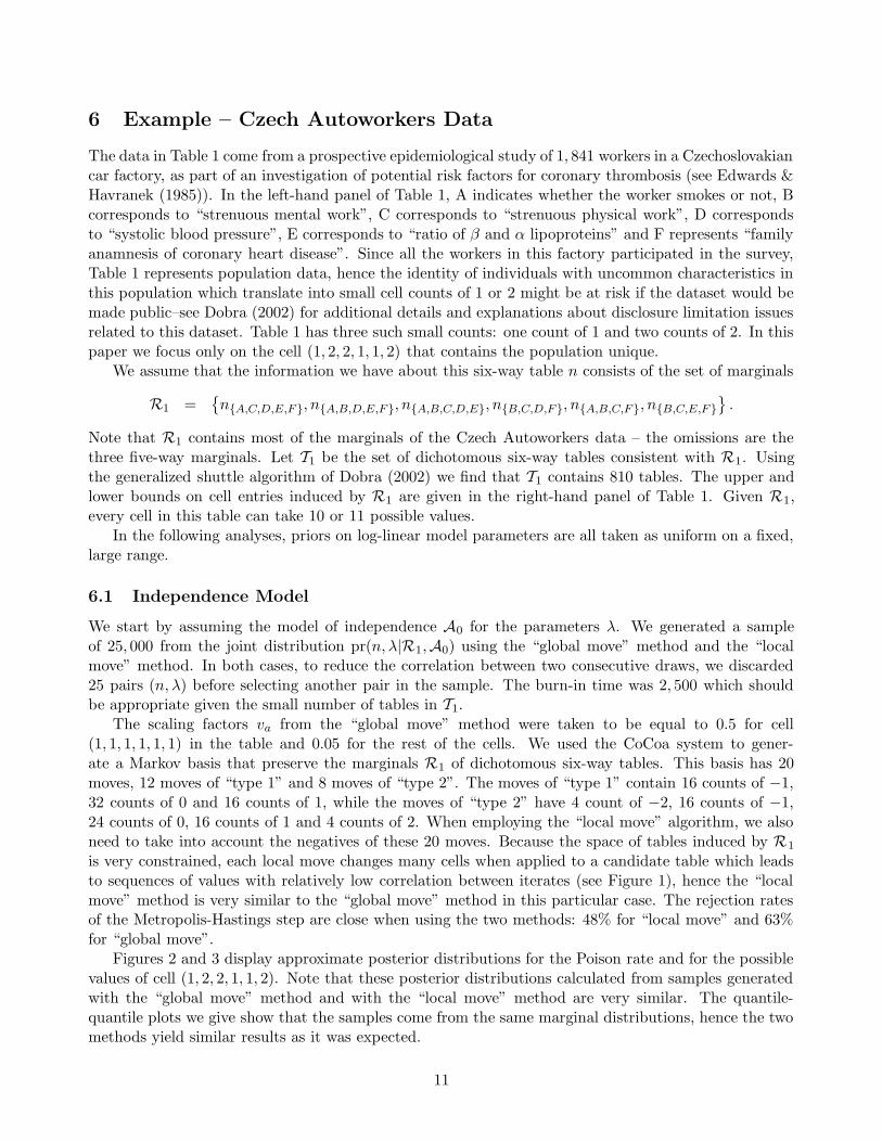
is very constrained, each local move changes many cells when applied to a candidate table which leadsto sequences of values with relatively low correlation between iterates (see Figure 1), hence the “localmove” method is very similar to the “global move” method in this particular case. The rejection ratesof the Metropolis-Hastings step are close when using the two methods: 48% for “local move” and 63%for “global move”.

Figures 2 and 3 display approximate posterior distributions for the Poison rate and for the possiblevalues of cell (1, 2, 2, 1, 1, 2). Note that these posterior distributions calculated from samples generatedwith the “global move” method and with the “local move” method are very similar. The quantile-quantile plots we give show that the samples come from the same marginal distributions, hence the twomethods yield similar results as it was expected.

11

0 50 100 150 200 250 300

0.0

0.4

0.8

Lag

ACF

Global Moves

0 50 100 150 200 250 300

0.0

0.4

0.8

Lag

ACF

Local Moves

Figure 1: Autocorrelation plots for the Poisson rate associated with the cell (1, 2, 2, 1, 1, 2) of the CzechAutoworkers data if the “global move” method was employed (top) and if the “local move” method wasemployed (bottom).

6.2 The Hypergeometric Distribution

Since T1 is small enough to enumerate all its elements, we were able to compute exactly the hypergeo-metric distribution induced by fixing the marginals R1–see (6). In the first row of Table 2 we presentthe exact marginal distribution for cell (1, 2, 2, 1, 1, 2) obtained from the hypergeometric. We can seethat this marginal distribution is unimodal and that the cell values 0, 1, 2, 3, 4 and 5 receive almostall the probability mass. The marginal probabilities for the other five possible values of this cell arestrictly positive, but they are very small.

We approximated the exact marginal of hypergeometric distribution for cell (1, 2, 2, 1, 1, 2) by gen-erating samples of size 10, 000 using three methods: (a) direct sampling from hypergeometric; (b) the“global move” method and (c) the “local move” method. The results are displayed in the second, thirdand fourth rows of Table 2. We see that all three methods yield reasonable good approximations of the“true” exact probabilities. The values 6, 7, 8, 9 and 10 were never obtained when sampling directlyfrom the hypergeometric and when the “global move” method was used. When using the “local move”method, the value 6 was generated once.

The scaling factors va for the “global move” method were all equal to 0.25 which induce a rejectionrate of 69%. The same Markov basis as before was used for the “local move” method. In this case therejection rate was 64%. For both imputation methods the burn-in time was 2, 500 and the gap betweentwo consecutive draws selected in the samples was 25.

6.3 Log-linear Models

In Section 3 we argued that the log-linear models A we need to consider in order to obtain differentposterior distributions pr(n|D,A, ·) are those log-linear models whose minimal sufficient statistics embedthe set of fixed marginals which constitute part or all the available information D. If the marginalsR1 are fixed, the set of relevant log-linear models is given in Table 3. Again, the hypergeometric

12

0 5 10 15 20

0.00

0.02

0.04

0.06

0.08

0.10

0.12

0.14

(a)

0 5 10 15

0.00

0.05

0.10

0.15

(b)

0 5 10 15 20

05

1015

2025

(c)

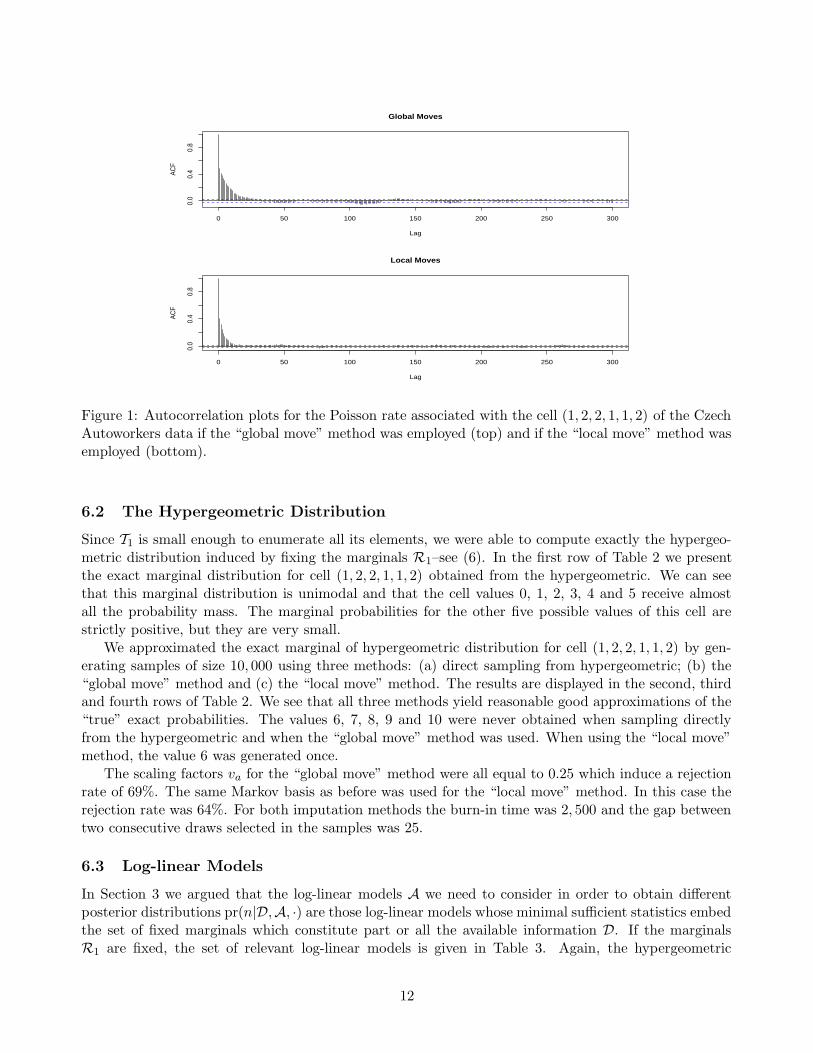
Figure 2: Marginal posterior distributions under the model of independence A0 for the Poisson rateassociated with cell (1, 2, 2, 1, 1, 2) of the Czech Autoworkers data obtained using (a) Global moves and(b) Local moves. A quantile-quantile plot of the samples obtained using the two methods is presentedat (c): the vertical axis represents the “global move” sample, while the horizontal axis represents the“local move” sample.

distribution is obtained by conditioning on a log-linear model whose marginals are embedded in the setof fixed marginals R1.

Using the “global move” method, we simulated a samples of size 25, 000 from the joint distributionspr(n, λ|R1,Aj) for each j = 1, 2, . . . , 8. The simulation details (e.g., burn-in time, scaling factors,rejection rates, etc) were very similar as in the case of independence model A0.

In Table 4 we summarized the approximate marginal posterior distributions for cell (1, 2, 2, 1, 1, 2)obtained by conditioning on the model of independence A0 (first row in the table), on any log-linearmodel whose marginals are known from R1 which leads to the hypergeometric distribution (secondrow) and on the “relevant” log-linear models A1, . . . ,A8 (third row up to tenth row). We note thatthese marginal distributions can be very different. In some instances, these distributions appear to beunimodal (with a mode at 0 or 2), while in some other instances, the posteriors seem to be bimodal(with a mode at 0 and another mode at 10).

7 Counting Tables

The “global move” method for sampling tables consistent with a set of constraints can be employed toestimate the total number of tables consistent with these constraints. Write M(T ) for the number oftables in the constrained set T . Chen (2001) suggested that M(T ) can be estimated by sampling fromthe uniform distribution on T , i.e., pr(n|D) = 1/M(T ), but this is infeasible in any but trivial problemssince it would be equivalent to knowing M(T ) exactly. Instead, we simulate tables from the proposaldistribution defined in (11) with scaling factors va equal (at least eventually) to 1 for all the cells in thetable. This particular choice of the scaling factor makes this proposal distribution independent of the

13

0 1 2 3 4 5 6 7 8 9 10

(a)

0.00

0.05

0.10

0.15

0 1 2 3 4 5 6 7 8 9 10

(b)

0.00

0.05

0.10

0.15

0 2 4 6 8 10

02

46

810

(c)

Figure 3: Marginal posterior distributions under the model of independence A0 for the possible values ofcell (1, 2, 2, 1, 1, 2) of the Czech Autoworkers data obtained using (a) Global moves and (b) Local moves.A quantile-quantile plot of the samples of cell values obtained using the two methods is presented at (c):the vertical axis represents the “global move” sample, while the horizontal axis represents the “localmove” sample.

table previously sampled, i.e.,

q(n) ∝m∏

a=1

1

U(n; ia) − L(n; ia) + 1.

Then, we can write

1 =∑

n∈T

pr(n|D)

q(n)q(n) =

1

M(T )

∑

n∈T

1

q(n)q(n).

This suggests an estimate for M(T ) given by

1

S

S∑

s=1

1

q(n(s))= S−1

S∑

s=1

m∏

a=1

[U(n(s); ia) − L(n(s); ia) + 1], (12)

where n(1), n(2), . . . , n(S) are sampled independently from q(·). As an example, consider two sets ofmarginals of the Czech Autoworkers data. For the first set we can count the exact number of tableswith a modified version of the generalized shuttle algorithm (Dobra, 2002); for the second, there are somany feasible tables and the generalized shuttle algorithm is infeasible.

Let R2 be the 15 four-way marginals of the Czech Autoworkers data. The upper and lower boundsinduced by R2 are given in the left-hand panel of Table 5. We generated 100 samples of 5, 000 tableseach from T2, the set of tables consistent with R2–see Figure 4. The true number of tables in T2 is705,884. The mean of our estimates of M(T2) is 703, 126 with a coefficient of variation of 0.0012,suggesting a very efficient sampling method. A 95% confidence interval for M(T2) is 651,919–750,234.

14

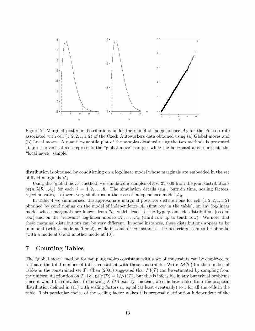
The second example assesses the number of dichotomous six-way tables that have a count of 1 incell (1, 2, 2, 1, 1, 2) (which identifies the population unique in the Czech Autoworkers data n) and thatare consistent with the marginals R3 given in (13),

R3 := {n{B,F}, n{A,B,C,E}, n{A,D,E}}. (13)

Let T3 denote this set of tables. The upper and lower bounds associated with T3 are given in the right-hand panel of Table 5. We generated 1, 000 samples of 35, 000 tables each–see Figure 4. We work onthe log10 scale as M(T3) is very large. The mean of log10{M(T3)} is 58 with a coefficient of variation of0.00005, and a 95% confidence interval of 57.60–59.31. The true number of tables M(T3) is, of course,unknown, but we have confidence in the estimate of 57 − 59.

600000 650000 700000 750000 8000000.0e

+00

5.0e

−06

1.0e

−05

1.5e

−05

(a)

56 57 58 59 60

0.0

0.2

0.4

0.6

0.8

1.0

(b)

Figure 4: Estimates for (a) M(T2) and (b) log10{M(T3)}.

8 Concluding Comments

Combined parameter inference and missing-data imputation in contingency tables is a very broad reach-ing problem. The specific context of inference based on data in terms of subsets of marginal countsis pervasive, and is central in problems of data disclosure, dissemination and confidentiality. Issues ofprior specification are relevant both for direct analysis, and in connection with questions about potentialuses of data released to multiple consumers who will each bring their own priors, or classes of priors,to bear on interpreting the margins. Our work describes some of the basic theoretical and structuralissues in the context of log-linear models, and presents a detailed development of MCMC approaches,with examples.

Central to the work reported is the development and implementation of Bayesian inference under aspecific class of structured priors for log-linear model parameters, and the introduction and developmentof a “global move” simulation approach for imputing missing elements of contingency tables subject toobserved margins. Our examples illustrate the use of both “local” and “global” move algorithms forsampling tables. Each has advantages and disadvantages, though we generally prefer the “global move”approach as it is relatively easily set up and implemented. The speed of the above procedure is directly

15

influenced by the number of cells that need to be fixed at a certain value before a full table consistentwith the data D is determined. Every time we assign a value to a cell, we need to update the upperand lower bounds for the rest of the cells in the table. Consequently, the smaller the number of cells weneed to fix, the faster the algorithm is. This number is a function of the pattern of constraints inducedby the full information D.

One of the requirements of the “global move” approach sampling algorithm is that the boundsdefining the values a cell count can take given data D and given that some other cells have been fixedat a certain value have to be sharp. Gross bounds approximating the corresponding sharp bounds willfrequently lead to combinations of cell values that do not correspond to tables in T , and hence theuse of gross bounds will significantly decrease the efficiency of this sampling procedure. Unfortunately,computing sharp bounds to determine the admissible values of every cell in the target table couldbecome a serious computational burden in the case of large high-dimensional tables having thousandsor possibly millions of cells. Therefore, one very difficult computational problem (the generation of aMarkov basis) from the “local move” algorithm is replaced, in the “global move” algorithm, with anothervery challenging problem–the calculation of sharp integer bounds. As we pointed out before, even ifsharp bounds are calculated and used at each step, there is no theory which shows that infeasiblecombinations of cell values cannot be generated. However, this has never happened in a range ofexamples studied so far. Note that the “local move” method generates candidate tables that are outsideT if a move that is not permissible for the current state of the chain is selected. In this respect, the“global move” method seems to perform better than the “local move” method.

In addition, a simulation algorithm employing the “global move” method can be started right awaywithout any possibly tedious preliminary computations required in most cases by the “local move”method. There are situations when the generation of a Markov basis could take too long to complete(hence no samples can be drawn with the “local move” method), while the “global move” method mightstill be applied and samples will still be generated even if these samples might be expensive in term ofcomputing time.

As opposed to the “local move” method that modifies only some small subset of cells affected by thechosen local move, the “global move” method potentially changes the entire table at each step, whichleads to sequences of tables with very low correlation from one step to the next, and clearly facilitatesan effective exploration of the multidimensional support of the random variables in exam.

Throughout the paper we employed the generalized shuttle algorithm (Dobra, 2002) to computesharp upper and lower bounds. This is a very flexible algorithm that allows one to specify differenttypes of constraints on the cell entries of a table. These constraints can be, but are not limited to, fixedmarginals or cells fixed at a certain value. Moreover, the generalized shuttle algorithm can be modifiedto exhaustively enumerate the tables consistent with a set of constraints.

We have illustrated how posterior inferences on cell counts can vary substantially based on assumedforms of log-linear models. It may in future be of interest to consider extensions of this work tobuild analyses across models, utilising model-mixing and model-averaging ideas (Kass & Raftery, 1995;Madigan & York, 1995), and some further developments of the proposed MCMC methods here thatextend to reversible-jump methods will be relevant there.

Acknowledgments

We thank Stephen Fienberg for comments and useful discussions, and Ian Dinwoodie for assistanceand advice on the generation of Markov bases. Elements of this work formed part of the StochasticComputation program (2002-03) at the Statistical and Applied Mathematical Sciences Institute, RTP,USA. Partial support was also provided under NSF grant DMS-0102227.

16

References

Agresti, A. (1992). A survey of exact inference for contingency tables. Statist. Sci. 7, 131–177.

Chen, Y. (2001). Sequential importance sampling and its applications. Ph.D. thesis, Stanford University.

Diaconis, P. & Efron, B. (1985). Testing for independence in a two-way table: new interpretationsof the chi-square statistic. The Annals of Statistics 13, 845–874.

Diaconis, P. & Sturmfels, B. (1998). Algebraic algorithms for sampling from conditional distribu-tions. The Annals of Statistics 26, 363–397.

Dobra, A. (2002). Statistical tools for disclosure limitation in multi-way contingency tables. Ph.D.thesis, Department of Statistics, Carnegie Mellon University.

Dobra, A., Fienberg, S. E. & Trottini, M. (2003). Assessing the risk of disclosure of confidentialcategorical data (with discussion). In Bayesian Statistics 7, J. M. Bernardo, M. J. Bayarri, J. O.Berger, A. P. Dawid, D. Heckerman, A. F. M. Smith & M. West, eds. Oxford University Press.

Edwards, D. E. & Havranek, T. (1985). A fast procedure for model search in multidimensionalcontingency tables. Biometrika 72, 339–351.

Haberman, S. J. (1974). The Analysis of Frequency Data. Chicago: University of Chicago Press.

Kass, R. E. & Raftery, A. E. (1995). Bayes factors. Journal of the American Statistical Association

90, 773–795.

Lauritzen, S. L. (1996). Graphical Models. Oxford: Clarendon Press.

Liu, J. S. (2001). Monte Carlo Strategies in Scientific Computing. New York: Springer.

Madigan, D. & York, J. (1995). Bayesian graphical models for discrete data. International Statistical

Review 63, 215–232.

Smith, P., Forster, J. & McDonald, J. (1996). Monte carlo exact tests for square contingencytables. Journal of the American Statistical Association 2, 309–321.

Sundberg, R. (1975). Some results about decomposable (or markov-type) models for multidimensionalcontingency tables: distribution of marginals and partitioning of tests. Scandinavian Journal of

Statistics 2, 71–79.

Tebaldi, C. & West, M. (1998a). Bayesian inference on network traffic using link count data (withdiscussion). Journal of the American Statistical Association 93, 557–576.

Tebaldi, C. & West, M. (1998b). Reconstruction of contingency tables with missing data. ISDSDiscussion Paper #98–01, Duke University.

West, M. (1997). Statistical inference for gravity models in transportation flow forecasting. TechnicalReport #60, National Institute of Statistical Sciences.

Whittaker, J. (1990). Graphical Models in Applied Multivariate Statistics. NewYork: John Wiley &Sons.

17

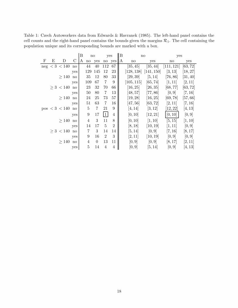
Table 1: Czech Autoworkers data from Edwards & Havranek (1985). The left-hand panel contains thecell counts and the right-hand panel contains the bounds given the margins R1. The cell containing thepopulation unique and its corresponding bounds are marked with a box.

B no yes B no yesF E D C A no yes no yes A no yes no yes

neg < 3 < 140 no 44 40 112 67 [35, 45] [35, 44] [111, 121] [63, 72]yes 129 145 12 23 [128, 138] [141, 150] [3, 13] [18, 27]

≥ 140 no 35 12 80 33 [29, 39] [5, 14] [76, 86] [31, 40]yes 109 67 7 9 [105, 115] [65, 74] [1, 11] [2, 11]

≥ 3 < 140 no 23 32 70 66 [16, 25] [26, 35] [68, 77] [63, 72]yes 50 80 7 13 [48, 57] [77, 86] [0, 9] [7, 16]

≥ 140 no 24 25 73 57 [19, 28] [16, 25] [69, 78] [57, 66]yes 51 63 7 16 [47, 56] [63, 72] [2, 11] [7, 16]

pos < 3 < 140 no 5 7 21 9 [4, 14] [3, 12] [12, 22] [4, 13]

yes 9 17 1 4 [0, 10] [12, 21] [0, 10] [0, 9]

≥ 140 no 4 3 11 8 [0, 10] [1, 10] [5, 15] [1, 10]yes 14 17 5 2 [8, 18] [10, 19] [1, 11] [0, 9]

≥ 3 < 140 no 7 3 14 14 [5, 14] [0, 9] [7, 16] [8, 17]yes 9 16 2 3 [2, 11] [10, 19] [0, 9] [0, 9]

≥ 140 no 4 0 13 11 [0, 9] [0, 9] [8, 17] [2, 11]yes 5 14 4 4 [0, 9] [5, 14] [0, 9] [4, 13]

18

Table 2: Marginal associated with cell (1, 2, 2, 1, 1, 2) of the hypergeometric distribution induced byfixing the marginals R1. The exact as well as the estimated cell probabilities were rounded to thefourth decimal. We marked with a “–” the cell values that did not appear in a sample. The values7, . . . , 10 receive a probability weight very close to 0 and do not appear in the table.

Possible Cell Values0 1 2 3 4 5 6

Exact Distribution 0.0028 0.1022 0.4663 0.3697 0.0570 0.0016 0.0000Direct Sampling 0.0035 0.1051 0.4712 0.3637 0.0547 0.0018 –Global Moves 0.0032 0.1066 0.4553 0.3759 0.0561 0.0029 –Local Moves 0.0029 0.1085 0.4595 0.3734 0.0538 0.0018 0.0001

19

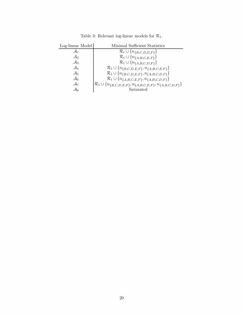
Table 3: Relevant log-linear models for R1.

Log-linear Model Minimal Sufficient Statistics

A1 R1 ∪ {n{B,C,D,E,F}}A2 R1 ∪ {n{A,B,C,E,F}}A3 R1 ∪ {n{A,B,C,D,F}}A4 R1 ∪ {n{B,C,D,E,F}, n{A,B,C,E,F}}A5 R1 ∪ {n{B,C,D,E,F}, n{A,B,C,D,F}}A6 R1 ∪ {n{A,B,C,E,F}, n{A,B,C,D,F}}A7 R1 ∪ {n{B,C,D,E,F}, n{A,B,C,E,F}, n{A,B,C,D,F}}A8 Saturated

20

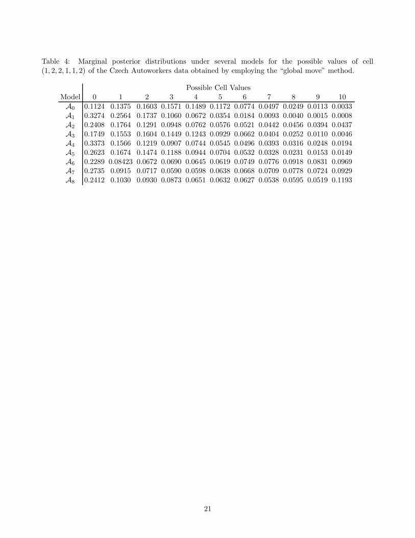
Table 4: Marginal posterior distributions under several models for the possible values of cell(1, 2, 2, 1, 1, 2) of the Czech Autoworkers data obtained by employing the “global move” method.

Possible Cell ValuesModel 0 1 2 3 4 5 6 7 8 9 10

A0 0.1124 0.1375 0.1603 0.1571 0.1489 0.1172 0.0774 0.0497 0.0249 0.0113 0.0033A1 0.3274 0.2564 0.1737 0.1060 0.0672 0.0354 0.0184 0.0093 0.0040 0.0015 0.0008A2 0.2408 0.1764 0.1291 0.0948 0.0762 0.0576 0.0521 0.0442 0.0456 0.0394 0.0437A3 0.1749 0.1553 0.1604 0.1449 0.1243 0.0929 0.0662 0.0404 0.0252 0.0110 0.0046A4 0.3373 0.1566 0.1219 0.0907 0.0744 0.0545 0.0496 0.0393 0.0316 0.0248 0.0194A5 0.2623 0.1674 0.1474 0.1188 0.0944 0.0704 0.0532 0.0328 0.0231 0.0153 0.0149A6 0.2289 0.08423 0.0672 0.0690 0.0645 0.0619 0.0749 0.0776 0.0918 0.0831 0.0969A7 0.2735 0.0915 0.0717 0.0590 0.0598 0.0638 0.0668 0.0709 0.0778 0.0724 0.0929A8 0.2412 0.1030 0.0930 0.0873 0.0651 0.0632 0.0627 0.0538 0.0595 0.0519 0.1193

21

Table 5: Bounds for the Czech Autoworkers data given the marginals R2 (left-hand panel) and giventhe marginals R3 (right-hand panel). The bounds for the cell (1, 2, 2, 1, 1, 2) are marked with a box.These bounds were calculated using the generalized shuttle algorithm.

B no yes B no yesF E D C A no yes no yes A no yes no yes

neg < 3 < 140 no [27, 58] [25, 56] [96, 134] [44, 82] [0, 88] [0, 62] [0, 224] [0, 117]yes [108, 149] [123, 168] [0, 22] [9, 37] [0, 261] [0, 246] [0, 24] [0, 38]

≥ 140 no [22, 49] [0, 24] [60, 96] [16, 52] [0, 88] [0, 62] [0, 224] [0, 117]yes [91, 127] [45, 85] [0, 18] [0, 20] [0, 261] [0, 151] [0, 24] [0, 38]

≥ 3 < 140 no [10, 37] [17, 44] [48, 86] [49, 89] [0, 58] [0, 60] [0, 170] [0, 148]yes [30, 68] [58, 102] [0, 19] [0, 25] [0, 115] [0, 173] [0, 20] [0, 36]

≥ 140 no [13, 37] [8, 36] [55, 90] [38, 76] [0, 58] [0, 60] [0, 170] [0, 148]yes [30, 67] [45, 86] [0, 19] [0, 27] [0, 115] [0, 173] [0, 20] [0, 36]

pos < 3 < 140 no [0, 15] [0, 13] [4, 31] [0, 23] [0, 88] [0, 62] [0, 125] [0, 117]

yes [0, 21] [3, 30] [0, 10] [0, 9] [0, 134] [0, 134] [1, 1] [0, 38]

≥ 140 no [0, 11] [0, 10] [0, 24] [0, 18] [0, 88] [0, 62] [0, 125] [0, 117]yes [0, 26] [2, 30] [0, 11] [0, 9] [0, 134] [0, 134] [0, 24] [0, 38]

≥ 3 < 140 no [1, 14] [0, 9] [0, 26] [0, 26] [0, 58] [0, 60] [0, 125] [0, 125]yes [0, 19] [4, 29] [0, 9] [0, 9] [0, 115] [0, 134] [0, 20] [0, 36]

≥ 140 no [0, 9] [0, 9] [0, 26] [0, 22] [0, 58] [0, 60] [0, 125] [0, 125]yes [0, 19] [0, 23] [0, 9] [0, 13] [0, 115] [0, 134] [0, 20] [0, 36]

22