Bayesian Inference for Geostatistical Regression Models Devin S. Johnson 1 Department of Mathematics and Statistics and Institute of Arctic Biology, University of Alaska Fairbanks July 18, 2005 1 E-mail: ff[email protected]; Address: Devin S. Johnson, Department of Mathematics and Statistics, P.O. Box 756660, University of Alaska Fairbanks, Fairbanks, AK 99775

Welcome message from author
This document is posted to help you gain knowledge. Please leave a comment to let me know what you think about it! Share it to your friends and learn new things together.
Transcript
Bayesian Inference for GeostatisticalRegression Models
Devin S. Johnson1
Department of Mathematics and Statisticsand
Institute of Arctic Biology,University of Alaska Fairbanks
July 18, 2005
1E-mail: [email protected]; Address: Devin S. Johnson, Department of Mathematics and Statistics,P.O. Box 756660, University of Alaska Fairbanks, Fairbanks, AK 99775
Abstract
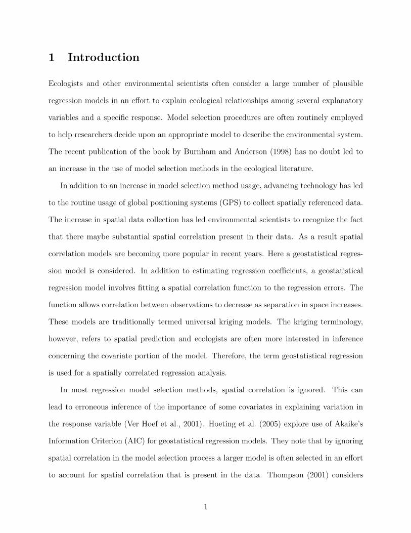
The problem of simultaneous covariate selection and parameter inference for spatial regres-sion models is considered. Previous research has shown that failure to take spatial correlationinto account can influence the outcome of standard model selection methods. Often, thesestandard criteria suggest models that are too complex in an effort to compensate for spatialcorrelation ignored in the selection process. Here calculation of parameter estimates andposterior model probabilities for regression models through a Markov Chain Monte Carlo(MCMC) method is investigated. In addition, the proposed MCMC algorithm is modifiedfor covariate selection in spatial generalized linear mixed models (GLMM). The GLMManalysis makes use of Langevin-Hastings updates for random effects. These methods aredemonstrated with two data sets, one normally distributed and the other a Poisson spatialGLMM.
Key words: Bayesian inference; generalized linear mixed models; geostatistics; Langevin-Hastings; model selection; Reverse Jump Markov Chain Monte Carlo
1 Introduction
Ecologists and other environmental scientists often consider a large number of plausible
regression models in an effort to explain ecological relationships among several explanatory
variables and a specific response. Model selection procedures are often routinely employed
to help researchers decide upon an appropriate model to describe the environmental system.
The recent publication of the book by Burnham and Anderson (1998) has no doubt led to
an increase in the use of model selection methods in the ecological literature.
In addition to an increase in model selection method usage, advancing technology has led
to the routine usage of global positioning systems (GPS) to collect spatially referenced data.
The increase in spatial data collection has led environmental scientists to recognize the fact
that there maybe substantial spatial correlation present in their data. As a result spatial
correlation models are becoming more popular in recent years. Here a geostatistical regres-
sion model is considered. In addition to estimating regression coefficients, a geostatistical
regression model involves fitting a spatial correlation function to the regression errors. The
function allows correlation between observations to decrease as separation in space increases.
These models are traditionally termed universal kriging models. The kriging terminology,
however, refers to spatial prediction and ecologists are often more interested in inference
concerning the covariate portion of the model. Therefore, the term geostatistical regression
is used for a spatially correlated regression analysis.
In most regression model selection methods, spatial correlation is ignored. This can
lead to erroneous inference of the importance of some covariates in explaining variation in
the response variable (Ver Hoef et al., 2001). Hoeting et al. (2005) explore use of Akaike’s
Information Criterion (AIC) for geostatistical regression models. They note that by ignoring
spatial correlation in the model selection process a larger model is often selected in an effort
to account for spatial correlation that is present in the data. Thompson (2001) considers
1
a Bayesian approach to geostatistical regression selection and model averaging predictions
using integral approximations to obtain the necessary quantities.
In this paper a Bayesian model selection procedure is investigated using a Markov Chain
Monte Carlo (MCMC) approach. Bayesian model selection, particularly the MCMC method
considered in this paper has many advantages over traditional methods such as AIC or
Bayesian methods using closed form approximations. Though a stochastic search of the
model space, modern computational techniques, such as Reverse Jump MCMC (RJMCMC)
(Green, 1995), allow model selection in cases where there is a large number of covariates
under consideration. This is typically difficult in the frequentist framework. In addition,
inference for the regression coefficients, accounting for model uncertainty, is a byproduct of
the RJMCMC approach. In the Bayesian paradigm model uncertainty has a straightforward
probabilistic interpretation. Model uncertainty is accounted for in the Bayesian paradigm
by allowing the model to vary as a random quantity (Clyde and George, 2004). Models,
or regression coefficients, are given a certain amount of a priori weight. The model is then
updated via Bayesian learning just as the parameters are in the classic Bayesian parameter
estimation framework to obtain the posterior distribution of the model. The prior weighting
of the coefficients is another benefit over frequentist methods such as AIC. Certain covariates
can be given more or less weight in determining the most appropriate model. Methods such
as AIC selection weight all covariates equally.
The posterior distribution of interest in Bayesian model inference is the joint distribution
of the model and the parameters for each model. A sample from this distribution is obtained
from the RJMCMC sampler and inference concerning regression parameters and the model
itself can be extracted from this sample. The RJMCMC approach also has one other major
advantage over AIC and Bayesian closed form approximations, it is directly extendable to
spatial generalized linear mixed models (GLMM). This implies the RJMCMC approach can
be an all purpose tool for geostatistical regression inference for Gaussian and non-Gaussian
2

data.
The paper proceeds as follows. In Section 2 the geostatistical regression model is fully
described along with a broad description of Bayesian estimation procedures for the model.
In Section 3 an RJMCMC method is described for selecting covariates in a spatial regression
model. Extension to the case of non-Gaussian data is described in Section 4 through the use
of a spatial generalized linear mixed model (GLMM). In Section 5 the proposed methods are
demonstrated with two data sets, one Gaussian and the other Poisson distributed. Finally,
Section 6 provides a discussion as well as some additional considerations for RJMCMC
selection of spatial regressions.
2 Geostatistical regression models
The geostatistical model (Cressie, 1993) is a commonly used model for spatially referenced
data in a continuous domain. Under the geostatistical framework the response variable of
interest may be sampled at random or predetermined locations. The variability in the mea-
sured response results from the random realization of the spatial field, not the randomness
of the sampling locations.
2.1 Model specification
Let Z = (Z(s1), . . . , Z(sn))′ be a set of spatially referenced observations. Technically, Z is
a partial realization of a random field Z(s), s ∈ D where D ⊂ R2 is a fixed, finite-sized,
domain or study area. A geostatistical regression model for relating a set of covariates to
the observation field is modeled as
Z(s) = x′(s)β + δ(s), (1)
where x(s) = (x0(s), . . . , xp(s))′ is a vector of known spatially referenced covariates, β is a
vector of unknown regression coefficients, and δ(s), s ∈ D is an unknown realization from
3

a zero-mean random field over D. It is usual practice to set x0(s) = 1 to obtain an intercept
parameter. The model in (1) is often referred to as a universal kriging model.
In order to fully specify the spatial regression, a spatial covariance model must be specified
for the error process δ(s). Herein, the spatial error process is assumed to be a stationary
Gaussian process with a spatial covariance of the form
Covδ(s), δ(s + h) = σ2ρ(h′Φh)
varδ(s) = σ2 + τ 2
(2)
where ρ is an isotropic correlation function, Φ is a 2 × 2 positive definite matrix, τ 2 > 0 is
a nugget parameter, and σ2 > 0 is the partial sill parameter. The nugget parameter allows
for extra variability in the response variable at each site. This may result from measurement
error or other latent processes which may produce a response variable surface that is not
smooth. In practice, most spatial data usually contain this extra variability (Diggle et al.,
1998). There are many forms that the correlation function ρ(·) may take. Typical choices
are the exponential, Matern, or spherical correlation functions (see Bailey and Gatrell (1995)
and Stein (1999)).
2.2 Parameter estimation
In this section, a Bayesian approach to parameter estimation is explored as a precursor to
Bayesian model selection. Bayesian estimation methods for spatial models are explored in
depth for isotropic models (Φ diagonal with equal entries) in Berger et al. (2001) and Hand-
cock and Stein (1993). Ecker and Gelfand (1999) propose a Bayesian method of inference
for anisotropic models. First the density of the data Z given the parameters (β, σ2, τ 2,Φ) is
needed. For a Gaussian field this is given by
P (Z|β, σ2, τ 2,Φ) ∝ |Σ|−1/2 exp
−1
2(Z−Xβ)′Σ−1(Z−Xβ)
, (3)
4
where X is the n × p design matrix of covariates, Σ is the covariance matrix with (i, j)
element defined by (2).
In addition to the data distribution a prior distribution for the parameters is also neces-
sary. For the regression parameters, the conditional conjugate distribution is the multivariate
normal distribution; often with the covariance matrix proportional to the variance of the re-
sponse variable P (β|σ2, τ 2) = N(µ, (σ2 +τ 2)Ω). This is the distribution that is used for the
examples in section 5. Due to the additive variance of the partial sill, σ2, and the nugget,
τ 2, there is no conjugate distribution for either of these parameters. Furthermore, previous
MCMC analysis of spatial data has noted a high posterior correlation between these two
parameters making MCMC samplers slow to converge (Christensen et al., 2005). Therefore,
the alternate parameterization θ1 = log(σ2) and θ2 = log(τ 2) is used. This was found to sig-
nificantly reduce correlation in the MCMC samples for the examples in Section 5. Since τ 2 is
often interpreted as independent measurement error a priori independence of the parameters
is assumed and Gaussian priors used P (θ1, θ2) = N(η1, ν1)N(η2, ν2)
The prior distribution for Φ needs some consideration. Because Φ needs to remain
positive definite, the first choice for a prior is often the Wishart distribution. This is the
prior proposed by Ecker and Gelfand (1999). The Wishart is rather inflexible, however, due
to a single “degrees of freedom” parameter. Therefore, the following reparameterization and
associated prior is proposed that seems quite flexible as a prior and allows univariate updating
if desired. First, factor Φ as Φ = AΨA, where A is a diagonal matrix with positive elements
and Ψ is a positive definite correlation matrix. Let α = (α1, α2)′ = (log(A11)/2, log(A22)/2)′.
Since any α ∈ R2 is valid, a sensible prior for α is a normal distribution P (α) = N(γ,Λ).
Due to the fact that Φ is a 2 × 2 correlation matrix, it has but one parameter ψ that
represents the angle of anisotropy. The valid range of ψ in that case is (-1, 1), therefore, a
noninformative prior is a uniform distribution P (ψ) = U(−1, 1). It was found in the example
data analyzed however, that as the MCMC sampler wanders towards ±1 numerical problems
5
are encountered. Therefore, a more sensible choice for a prior is one that puts less mass near
the boundaries. In Section 5 a triangle distribution centered at 0 is used with good results.
The elements of the original anisotropy matrix Φ can be rewritten as functions of α and ψ
Φii = expαi for i = 1, 2
Φij = ψ exp(αi + αj)/2 for i 6= j.
If the dimension of the coordinates is larger than 2, Barnard et al. (2000) provide a possible
prior choice for Ψ.
Bayesian inference for the spatial regression model is based on the posterior distribution
P (β, θ1, θ2,α, ψ|Z) ∝ P (Z|β, θ1, θ2,α, ψ)
× P (β|θ1, θ2)P (θ1)P (θ2)P (α)P (ψ).
(4)
Desired quantities for summarization of the density are usually in the form of expected
values, for example posterior means, variances, and percentiles or credible intervals. The
posterior density in (4) is intractable, therefore, these quantities must be approximated from
an MCMC sample. One can employ the Gibbs sampler (see Robert and Cassella (1999) for
general MCMC and Gibbs sampler description) to accomplish this task.
3 Bayesian selection of geostatistical models
Here a method is presented for selection of covariates in a spatial regression model under the
Bayesian paradigm. The Bayesian method for model selection is largely appealing due to its
wide applicability. For virtually any statistical model, the Bayesian approach can be applied.
In addition, modern MCMC procedures such as Reverse Jump MCMC (RJMCMC) allow
application of the Bayesian approach even when the model space is large (i.e. thousands
of models considered) Clyde and George (2004), Hoeting et al. (1999), and Raftery et al.
(1997) provide overviews of the Bayesian approach to model selection.
6
3.1 Bayesian model uncertainty
The Bayesian approach to model uncertainty assumes that the model itself, like the pa-
rameter values, are an unknown entity. Therefore, the joint posterior distribution of the
parameters and the model are of interest. This joint posterior is given by
P (ϑk,mk|Z) ∝ P (Z|ϑk,mk)P (ϑk|mk)P (mk), (5)
where ϑk are the parameters for each model mk (in the spatial regression case, ϑk =
(β′k, θ1, θ2,α, ψ)′) and P (mk) is the prior distribution of the model set M = m0, . . . , mK.A classic model prior for regression analysis is derived by treating inclusion of the p coef-
ficients as a series of independent Bernoulli trials with probability πj, j = 1, . . . , p (Clyde
and George, 2004). The result is the following prior
P (mk) =
p∏j=1
πIj
j (1− πj)1−Ij , (6)
where Ij is an indicator that covariate j is included in the regression model. This prior
includes the uniform prior P (mk) = 1/2p; obtained by setting πj = 1/2, j = 1, . . . , p.
In most model selection problems the object of inference is not the joint model-parameter
posterior, it is the marginal posterior distribution of the model M . This marginal distribution
is the posterior model probability (PMP);
P (mk|Z) ∝∫
P (Z|ϑk,mk)P (ϑk|mk)P (mk)dϑk
= P (Z|mk)P (mk).
(7)
The PMP is almost always unobtainable in closed form. Typically, the model with the
largest PMP is selected (although, see Barbieri and Berger (2005) for selection based on the
median posterior model). Alternatively, one may not want to select a specific model, but use
all of the models, appropriately weighted by their PMPs, in an ensemble fashion. Hoeting
et al. (1999) provide a detailed description of this type of inference termed Bayesian Model
Averaging (BMA).
7
This paper will use both BMA and maximum PMP to make inference concerning im-
portance of each covariate in explaining an ecological or environmental response. It is self
apparent that the maximum PMP model will provide information on important covariates.
Another quantity, Posterior Inclusion Probabilities (PIP), are also useful in regression set-
tings. The PIP for each covariate is defined as
P (βj 6= 0|Z) =∑
k:βj 6=0
P (mk|Z). (8)
This is the model averaged posterior probability of inclusion of the jth covariate. The PIP
for each covariate provides a measure of importance of each covariate to the response.
3.2 RJMCMC implementation
Unlike ordinary regression, the PMPs and PIPs are unobtainable in closed form in the spatial
regression case. Therefore, a MCMC approach can be used. Green (1995) proposes the
RJMCMC method for sampling from the joint space of the parameters and model. Sample
averages can then be used to approximate expected values of model and parameter functions,
such as PMPs and PIPs. The general RJMCMC method proceeds as follows for a current
state q = (ϑk,mk):
1. Draw proposal move of type i to mk∗ from distribution Ji(q)
2. Draw parameter proposal ϑk∗ from Gi(q,mk∗)
3. Accept new state q∗ with probability
min
1,
P (q∗|Data)Ji(q∗)Gi(q
∗,mk)
P (q|Data)Ji(q)Gi(q,mk∗)
. (9)
Typically, an RJMCMC algorithm involves several move types in order to obtain an ergodic
chain. Move types can be systematically or randomly selected. Both Metropolis-Hastings
and Gibbs samplers are special cases of RJMCMC (Green, 2003).
8
The major drawback of the general RJMCMC method is the double proposal necessary
to move to a different model. First, an appropriate model must be proposed, followed by
an acceptable proposal for the parameters of the model. If either of these two proposals is
inefficient then the chain will fail to mix well and a large number of iterations will be necessary
to obtain posterior model inference. A large number of MCMC iterations is exceptionally
difficult to handle in the spatial regression case due to the large covariance matrix Σ which
must be inverted.
In order to avoid long RJMCMC runs with spatial regression models an efficient proposal
scheme is necessary. Godsill (2001) suggests a general proposal method for model classes
where some of the parameters are shared among each model. In the spatial regression
case, the spatial parameters ξ = (θ1, θ2,α, ψ)′ are common to all of the models, whereas
βk differs for each model. If the conditional posterior distribution of the model given the
shared parameters is available than a Partial Analytic RJMCMC (PARJ) algorithm can be
constructed. Using the basic idea of Godsill, a PARJ chain can be constructed for spatial
regression model moves in the following manner. For a current state q = (βk,mk, ξ),
1. propose model move to mk∗ with probability J(mk∗),
2. propose βk∗ ∼ P (βk∗|mk∗ , ξ,Z),
3. set ξk∗ = ξ,
4. accept mk∗ with probability
min
1,
P (mk∗ |ξ,Z)J(mk∗)
P (mk|ξ,Z)J(mk)
. (10)
The acceptance ratio in (10) results from substitution of Gi(x) = P (βk∗ |mk∗ , ξ,Z) in (9)
and the identity
P (mk∗|ξ,Z) =P (βk,mk∗ |ξ,Z)
P (βk∗|mk∗ , ξ,Z).
Upon examination of (10), one can see there is no need to actually draw βk∗ proposal values
assuming the conditional distribution P (mk∗ |ξ,Z) is available up to its normalizing constant.
9
To obtain the acceptance probability ratio note that if P (βk|ξ) = N(µk,Vk), then, since
Z = Xkβk + δ, one obtains P (Z|ξ, mk) = N(Xkµk, XkVkX′k + Σ), where Σ = Cov(δ).
Hence,
P (mk|ξ,Z) ∝ exp
−1
2(Z−Xkµk)
′(XkVkX′k + Σ)−1(Z−Xkµk)
P (mk). (11)
Note, the suggested model proposal applies only to model jumps. Updates for the remain-
ing spatial parameters and regression parameters are necessary to obtain an ergodic chain.
Therefore, after model jumps one must update the spatial parameters ξ and the regression
coefficients with, perhaps, a Metropolis-within-Gibbs sampler.
4 Models and model selection for non-Gaussian data
If the response data is non-Gaussian, such as count data, it is typical to use a generalized
linear model for regression analysis. In order to account for spatial correlation, Diggle et al.
(1998) propose using a spatial GLMM. In a spatial GLMM the response variables, Y (s)
are assumed to be independent given an underlying Gaussian spatial field δ(s). That is to
say [Y|δ] is distributed according to the exponential family density∏n
i=1 P (·, µ(si)), where
E[Y (s)|δ(s)] = µ(s) = `−1x(s)′β + δ(s), where x(s) vector of covariates and `· is a
strictly increasing link function.
In its present form, the proposed PARJ algorithm in the previous section can not be
utilized. The βk vector cannot be integrated out of the likelihood portion of the model.
With a reparameterization, however, one can make use of the PARJ approach. The spatial
GLMM can be reformulated using a hierarchical centering approach (Gelfand et al., 1996)
and stated in the following fashion,
[Y|Z] ∼n∏
i=1
P (·, `−1Z(si))
[Z|β, ξ] ∼ N(Xβ, Σ),
(12)
10
where Σ is the spatial covariance matrix constructed from the spatial covariance parame-
ters ξ = (θ1, θ2,α, ψ)′. By changing the spatial process from a zero-mean error term to a
non-zero latent spatial process, the regression coefficient vector has been removed from the
likelihood model. The posterior density of the β vector remains the same, however, since the
reparameterization is a simple linear transformation with unit slope. Therefore, the essence
of the spatial GLMM remains unchanged. Although this reparameterization makes PARJ
updates possible it may not be appropriate for all data. See the discussion in Section 6 for
an explanation.
The PARJ approach to model selection can be utilized with the hierarchical centering pa-
rameterization by noting that β is independent of Y given the latent variables Z. Therefore,
the following model update is proposed for a current state q = (βk,mk, ξ,Z)
1. propose model move to mk∗ with probability J(mk∗),
2. propose βk∗ ∼ P (βk∗|mk∗ , ξ,Z),
3. set (ξk∗ ,Zk∗) = (ξ,Z),
4. accept mk∗ with probability (10), where P (mk|ξ,Z) is again given by (11)
As one can see, using the hierarchical centering, there is a direct extension to the GLMM spa-
tial regression case. Here, there is also no need to actually sample new regression coefficients
in the model updating step.
In addition to model updates, the parameters must be updated at each iteration to assure
an ergodic chain. So, before the model update each of the parameters βk, σ2, τ 2, α, and ψ
can be updated under the current model with their respective full conditional posterior
distributions which are independent of the data Y given the current state of Z.
The final step in the complete PARJ updating scheme for spatial GLMMs is to update
the latent process Z. The vector Z is often of high dimension (one element for each ob-
served site), so one must be careful is choosing an updating proposal. For high dimensional
updates it is often advisable to use Langevin-Hastings (LH) proposals (Christensen and
11
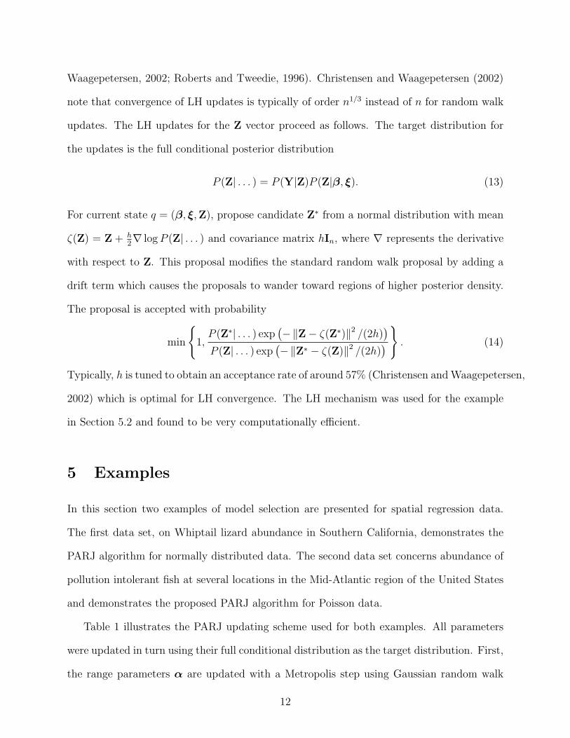
Waagepetersen, 2002; Roberts and Tweedie, 1996). Christensen and Waagepetersen (2002)
note that convergence of LH updates is typically of order n1/3 instead of n for random walk
updates. The LH updates for the Z vector proceed as follows. The target distribution for
the updates is the full conditional posterior distribution
P (Z| . . . ) = P (Y|Z)P (Z|β, ξ). (13)
For current state q = (β, ξ,Z), propose candidate Z∗ from a normal distribution with mean
ζ(Z) = Z + h2∇ log P (Z| . . . ) and covariance matrix hIn, where ∇ represents the derivative
with respect to Z. This proposal modifies the standard random walk proposal by adding a
drift term which causes the proposals to wander toward regions of higher posterior density.
The proposal is accepted with probability
min
1,
P (Z∗| . . . ) exp(−‖Z− ζ(Z∗)‖2 /(2h)
)
P (Z| . . . ) exp(−‖Z∗ − ζ(Z)‖2 /(2h)
)
. (14)
Typically, h is tuned to obtain an acceptance rate of around 57% (Christensen and Waagepetersen,
2002) which is optimal for LH convergence. The LH mechanism was used for the example
in Section 5.2 and found to be very computationally efficient.
5 Examples
In this section two examples of model selection are presented for spatial regression data.
The first data set, on Whiptail lizard abundance in Southern California, demonstrates the
PARJ algorithm for normally distributed data. The second data set concerns abundance of
pollution intolerant fish at several locations in the Mid-Atlantic region of the United States
and demonstrates the proposed PARJ algorithm for Poisson data.
Table 1 illustrates the PARJ updating scheme used for both examples. All parameters
were updated in turn using their full conditional distribution as the target distribution. First,
the range parameters α are updated with a Metropolis step using Gaussian random walk
12

proposal. Second, the anisotropy parameter ψ is updated with a Metropolis step using a
uniform random walk truncated to (-1, 1). Next, the log variance components, θ1 and θ2,
were each updated with random walk Metropolis steps. Following updates of the spatial
covariance parameters, the model mk was updated using the following proposal. First,
one of the covariate coefficients was selected with uniform probability 1/7. Second, if the
covariate was in the model, propose it for removal, if the covariate was not in the model
propose it for addition. In this proposal J(m) is symmetric in the model space, so the
acceptance probability is simply the ratio of equation (11) evaluated at the proposed model
over equation (11) evaluated at the current model. After model updates, the regression
coefficients βk were updated to the new model with a Gibbs update. The βk full conditional
distribution is Gaussian. Finally, for the Poisson data, a Langevin-Hastings step is used to
update the latent spatial process Z.
5.1 Abundance of Whiptail lizards in California
The proposed model selection methodology was applied to the whiptail lizard data set ini-
tially analyzed by Ver Hoef et al. (2001) using a stepwise procedure with a spatial correlation
correction. The data was subsequently analyzed by Thompson (2001), using a BIC approx-
imation to the PMP (Raftery, 1996), and Hoeting et al. (2005) using AIC. Each of these
analyses demonstrate the danger of ignoring spatial correlation when selecting covariates. A
larger model is often selected to account for the ignored correlation.
The data set is composed of abundance data of the Orange-throated whiptail lizard in
Southern California. At n = 149 locations where lizards were observed the average number
of lizards trapped during a week long trapping period was recorded. The response variable
analyzed is the log transformed value Z(s) = ln(average no. trapped at location s). Due to
the fact that several of the sites are very close to one another, one might suspect that the
same individuals might be trapped at different sites. This would lead to similar counts for
13
sites near each other; even in the absence of covariate effects.
Several covariates were collected to investigate which environmental conditions explain
lizard abundance. The original set of environmental covariates contained 37 variables. After
initial screening (Thompson, 2001) 6 covariates remained which held potential to explain
lizard abundance: Crematogaster ant abundance (3 levels - low, medium, high), log % sandy
soils, elevation, a bare rock indicator, % cover, and log % chaparral plants. Using indicators
for ant level 1 and 2, there are 128 possible models. All 6 covariates were normalized to have
mean zero and variance 1.
5.1.1 Model and prior distributions
The PARJ approach was used to select covariates with spatial correlation present. Here, the
full spatial model is used with nugget and anisotropy. The exponential function ρ(dij) =
exp−dij, where dij = h′ijAΨAhij was used to model spatial correlation. None of the pre-
vious analyses included anisotropy effects. In addition, a model without spatial correlation
was analyzed as well to determine any effects that might occur when correlation is ignored
in the selection process.
The priors described in Section 2.2 were used for the whiptail analysis. Following Thomp-
son (2001) and Raftery et al. (1997), the mean and variance of the β normal prior was chosen
to be µ = (Z, 0, . . . , 0), where Z the sample mean of Z. The prior covariance was chosen
to be Ω = 100(X′kXk)
−1. Priors for the variance parameters θ1 and θ2 where chosen to be
N(0, 10). A variance of 10 provided adequate coverage over the set of realistic values of the
partial sill and nugget. For each range parameter αi, a N(0, 1) prior distribution was used.
Automatically choosing extremely large variances for the range priors can put an unrealistic
amount of mass on ranges well beyond maximum observed distances, which can adversely
affect results. A variance of 1 seemed to adequately distribute prior mass over acceptable
ranges. Finally, as mentioned in Section 2.2, a uniform distribution can be used for a non-
14
informative prior on ψ, however, a triangular distribution over (-1, 1) and centered on 0
produced a more stable MCMC analysis. This was due to the fact that ψ values near ±1
tended to cause inconsistencies in the covariance structure.
The PARJ chain was run for 100,000 iterations following a sufficient burn-in period. In
order to judge whether this was acceptable, a means test was performed on the parameters
common to all models, as well as, the indicators of covariate inclusion in the model. Visual
inspection also confirmed that this was an acceptable chain length.
5.1.2 Model selection results
The top 5 models in PMP are given in Table 2. The PARJ algorithm visited 114 out of
128 possible models. The top model included Ant1 and log % Sandy Soil. With only 17.8%
posterior model mass, however, there is considerable uncertainty in the best model. When
ignoring spatial correlation the top spatial regression model ranks 5th in order with a PMP
of only 5.5%. Under the independence assumption, the top PMP model includes: Ant1, log
% sandy soil, and log % chaparral (PMP = 30.8%). Table 6 shows the PIPs for each of
the covariates. In addition, the table also shows the PIPs for the analysis without spatial
correlation. When, spatial correlation is accounted for log % sandy soil is the only covariate
with a PIP greater than 50%. When spatial correlation is ignored during the selection process
Table 6 illustrates that a different model inference is obtained. Without a spatial model Ant1
becomes a virtually certain inclusion and log % chaparral also enters as an important variable
along with log % sandy soil.
The difference in results should not be surprising. The fact that log % chaparral enters
the model in the independence case but is absent in the spatial model is most likely due
to a spurious regional effect. At nearby sites both the response and covariate are likely to
have similar values due the spatial correlation of each variable. In the sample, high response
values seem to be associated with high covariate values, but it is really the proximity of the
15
sites to one another that is driving the relationship. The same is also no doubt true for the
PIP increase in the Ant1 covariate.
The results obtained herein are similar to the previously mentioned analyses of this data.
Using an isotropic Matern model with nugget, Thompson (2001) noted that log % sandy
soil seemed to be the most important covariate. Hoeting et al. (2005) noted that the highest
AIC model contained Ant1 and log % sandy soil. While the MCMC analysis did not pick the
full model under the independence assumption as AIC does (Hoeting et al., 2005), certainly
more weight was placed on the other covariates. Using a spatial stepwise selection Ver Hoef
et al. (2001) also noted that the best model was one that contained ant abundance and log
% sandy soil.
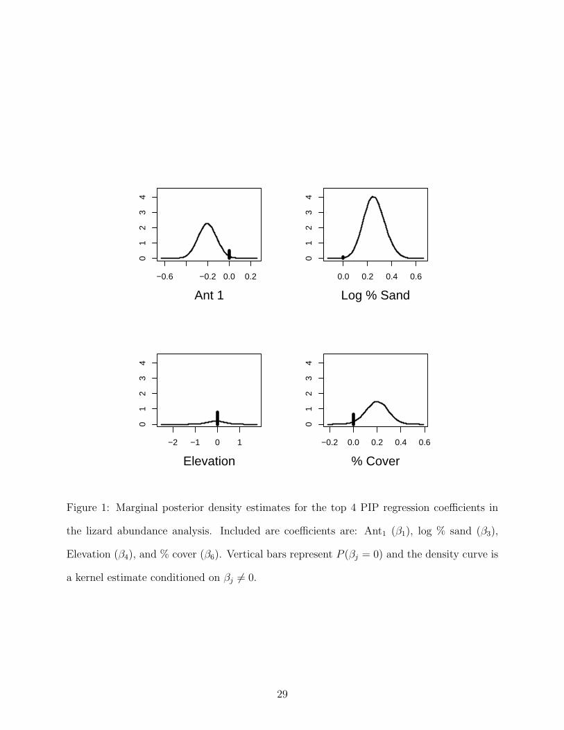
In addition to the model inference obtained through the PARJ method, Figure 6 shows the
marginal posterior density estimates for the top 4 PIP coefficients. Using these distributions
direction and magnitude of the covariate effects can be examined after accounting for model
uncertainty. Relative to high ant abundance, the presence of low ant abundance negatively
influences lizard abundance. This should be expected as the ants are the main prey source.
Lizard abundance is positively related to the % of sandy soil in the substrate. The remaining
coefficients, elevation and % cover, have smaller PIP as can be seen in Figure 6 by the size
of the bar relative to the density curve. Elevation seems to have neither strong positive or
negative influence as the density curve is centered at zero. There seems to be a positive
influence of % cover, but there is substantial probability (≈ 65%) that it is equal to zero.
5.2 Pollution Tolerance in Mid-Atlantic Highlands Fish
In 1994 and 1995 numerous stream sites in the Mid-Atlantic region of the Unites States
(Maryland, Pennsylvania, Virginia, West Virginia) were visited as part of the U.S. Envi-
ronmental Protection Agency’s EMAP water quality monitoring program. Several stream
characteristics were measured to assess water quality. At n = 119 sites, shown in Figure 2,
16
fish were sampled and classified according to their pollution tolerance. When assessing water
quality the abundance of pollution intolerant fish at a site is often a good index. In this
section a model selection analysis is performed to determine which of several environmental
factors contribute to overall abundance of pollution-intolerant fish.
5.2.1 Environmental covariates
The emphasis of the analysis is the effects of pollution and stream quality variables, how-
ever, there are several natural factors which might also influence abundance. The natural
covariates include Strahler stream order (ORDER) (a measure of stream size), elevation
(ELEV), and watershed area (WSA). The remaining covariates can be modified by human
use and, therefore, considered potential stream quality variables. Stream quality variables
included: road density in the watershed (RD) (No./area), % watershed classified as disturbed
by human activity (DISTOT), an index of fish habitat quality at the stream site (HAB),
concentration of dissolved oxygen in the stream at the sampling site (DO), % areal fish cover
at the sampling site (XFC), and % sand in stream bed substrate (PCT). The covariates in
this analysis have vastly different scales, therefore, to increase MCMC mixing, the covariates
were standardized to have mean 0 and variance 1.
It is believed a priori that the natural variables should be included in the final model,
but, this is not known with certainty. Therefore, the natural variables will be more heavily
weighted in the prior model probabilities. For the natural variables prior inclusion probabil-
ities were set to πj = 0.75, while for the remaining disturbance variables πj = 0.5. This a
priori weighting illustrates one of the advantages of the Bayesian approach to selection. In
addition, the data were also analyzed with a flat model prior (πj = 0.5 for all j) to examine
sensitivity of this prior weighting.
17
5.2.2 Model and prior distributions
A Poisson distribution with the canonical log link function is chosen for the abundance
model. So, the likelihood is given as
P (Y|Z) ∝119∏i=1
exp [Z(Si)Y (si)− expZ(si)] . (15)
This Poisson likelihood combined with the spatial model for the latent spatial process pro-
duces
ζ(Z) = Y − expZ −Σ−1(Z−Xkβk), (16)
for the drift term of the LH updates of Z. Heuristically a very sensible choice for drift, the
term a contrasts likelihood fit versus spatial fit. In the LH updates of Z, a value of h = 0.013
was used providing an acceptance rate of approximately 50%.
Priors for βk and log σ2 = θ1 were chosen to be N(0, 100σ2(X′kXk)
−1) and N(0, 10)
respectively. An isotropic exponential spatial correlation model was used for covariate se-
lection after initial analysis of the full model suggested no significant anisotropy or nugget
effect. The Poisson observation model essentially takes the place of the nugget measurement
error variability in the Gaussian process. A N(0, 1) was used as a prior for the single range
parameter α. For Gibbs updating of α a normal random walk proposal with variance tuned
to obtain an acceptance rate of approximately 30%.
The PARJ chain was run for 300,000 iterations after a sufficient initial burn-in. As in the
previous example, a random walk model proposal is used for the model updating stage of the
PARJ algorithm. After comparing several starting values for the parameters and model, as
well as a visual inspection of the marginal chains, it was determined that this was a sufficient
number of iterations. The PARJ analysis in this section actually took approximately the
same amount of time per iteration as the analysis in the previous section. So, the LH updates
of Z are computationally very fast and efficient as noted by Christensen and Waagepetersen
(2002).
18
5.2.3 Model selection results
During the analysis, the PARJ chain visited 419 out of 512 possible models. The top 5
models, as determined by PMP, are presented in Table 4. Upon examining the results
one can see that there is considerable uncertainty in deciding which is the best model.
The maximum a posterior model accounts for only 12.4% of the total probability mass in
the informative model and 17.8% of the mass in the flat prior analysis. The top PMP
model coincides in each analysis. Upon examination of Table 4 one can see that the models
containing WSA and ELEV in the informative prior analysis ranked lower and had smaller
PMP in the flat prior analysis. This suggests that WSA and ELEV are not as important
to intolerant fish abundance as was described by the informative prior. This also explains
the increase in maximum PMP. The data contradict the informative prior which leads to
an increase in model uncertainty. Table 5 shows that three covariates stand out as having
significant probability (> 0.5) of inclusion in the regression model, stream order (ORDER),
% watershed disturbed by human use (DISTOT), and habitat quality (HAB). The same
is true of the flat prior analysis. The PIPs are much smaller for ELEV and WSA than
the informative model prior, leading to the conclusion that they are not as important to
intolerant fish abundance a posteriori. All other covariates remain relatively unchanged in
PIP.
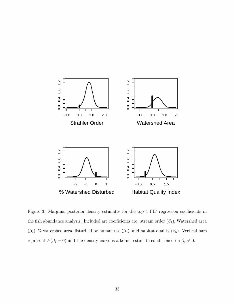
Figure 3 illustrates the estimated marginal posterior densities for the 4 parameters: OR-
DER, WSA, DISTOT, and HAB. ORDER is positively related to intolerant fish abundance.
WSA is also positively related to intolerant fish abundance, however, there is not strong
evidence of a significant effect. Abundance is negatively related to DISTOT and positively
related to HAB. Investigation of the scale of coefficient values for DISTOT and HAB shows
that DISTOT seems to have a larger magnitude effect than HAB, suggesting a larger ef-
fect of watershed scale disturbance over site level effects. In fact, the PARJ output can be
19

used to determine the model averaged posterior distribution of the ratio of the coefficients
for DISTOT to HAB. Unconditionally, the posterior probability that DISTOT has a larger
magnitude coefficient is 60.4%. Providing some evidence of a larger watershed level effect.
When both variables are included in the model, however, the 95% highest posterior proba-
bility interval for the ratio of absolute coefficient values is 0.00-4.93, indicating the evidence
is not strong.
6 Discussion
The results presented here demonstrate that general RJMCMC methodology can be mod-
ified to select covariates in spatial regressions through the partial analytic approach. The
method was presented for analysis of geometrically anisotropic data with a new prior specifi-
cation for the anisotropy parameters. The methodology does not require coefficient proposals
along with a model proposal. This eliminates one of the possible sources of model proposal
rejection. Model parameters are then updated through a series of Gibbs steps. In the spa-
tial GLMM scenario updates of the latent geostatistical process are also required. This is
efficiently accomplished through Langevin-Hastings proposals in a single block.
Analysis of the whiptail data set illustrates the common danger of ignoring spatial correla-
tion when selecting important covariates. Some covariates may seem important in modeling
the response when they are simply trying to account for spatial correlation. Readers are
cautioned, however, that it is not suggested that important covariates should be ignored
and relegated to spatial covariance. The goal of spatial regression is to investigate which
covariates are important. Therefore, if one or more of the covariates removes the spatial
correlation effects, then an independence model is probably more appropriate. This is not
the case for the whiptail data. The PARJ chain has an opportunity to explore the posterior
region with small spatial effects and coefficient values near those of the independence model.
20

The difference in selection results illustrates the significance of the spatial model.
On a cautionary note, Christensen et al. (2005) illustrates the fact that the hierarchical
centering necessary for the PARJ algorithm to work in the GLMM case may not work for all
data sets. In the Poisson case, if cell counts are very low for all sites or there are some sites
with extremely high counts and others with zero counts the LH updating and hierarchical
centering parameterization may produce chains that are slow to converge. This was not
a problem with the intolerant fish abundance data presented in Section 5, but researchers
using the PARJ method should examine their analysis with this in mind. The effect that
slow latent process and parameter convergence has on model chain convergence is the subject
on-going research. Christensen et al. (2005) propose a robust parameterization and MCMC
algorithm which looks promising for parameter estimation when the model is fixed. Their
method, however, is not immediately applicable to the PARJ approach. A modification of
their method is currently under investigation to determine if the PARJ algorithm can be
made more robust.
Another aspect of classic regression analysis for non-Gaussian continuous data is to ac-
count for uncertainty in power transformations. In terms of prediction in spatial models this
was addressed by Oliveira et al. (1997) in a Bayesian context. Theoretically, this is not a
problem for the PARJ algorithm presented herein. The likelihood involves one additional
parameter, the transformation power, that is mathematically common to all models. There-
fore, it can be conditioned upon in the model updating step just as the spatial parameters
are conditioned upon. Care must be taken, however, when specifying prior distributions for
the regression coefficients. The scale and interpretation of the coefficients depends on the
power of the transformation and they must be consistent for the analysis to make sense. In
the past Bayesian analysis with unknown transformations have focused on improper priors
for the regression coefficients (Box and Cox, 1964; Pericchi, 1981). Usually, proper priors are
necessary to obtain PMPs. Therefore, development of consistent proper priors is necessary
21
to use the PARJ approach.
Acknowledgements
The author would like to thank J. Ver Hoef and M. Stein for discussions and comments
that lead to an improved version of this manuscript. This work was partially funded by
STAR Research Assistance Agreement CR-829095 awarded to Colorado State University by
the U.S. Environmental Protection Agency. The views expressed here are solely those of
authors. EPA does not endorse any products or commercial services mentioned here.
References
Bailey, T. C. and Gatrell, A. C. (1995). Interactive Spatial Data Analysis. Prentice Hall,
New York.
Barbieri, M. M. and Berger, J. O. (2005). Optimal predictive model selection. Annals of
Statistics, (to appear).
Barnard, J., McCulloch, R., and Meng, X. L. (2000). Modeling covariance matrices in terms
of standard deviations and correlations, with application to shrinkage. Statistica Sinica,
10:1281–1311.
Berger, J. O., De Olivera, V., and Sanso, B. (2001). Objective Bayesian analysis of spatially
correlated data. Journal of the American Statistical Association, 96:1361–1374.
Box, G. E. P. and Cox, D. R. (1964). The analysis of transformations (with disscussion).
Journal of the Royal Statistical Society, Ser. B, 26:211–252.
Burnham, K. P. and Anderson, D. R. (1998). Model Selection and Inference: A Practical
Information-Theoretic Approach. Springer-Verlag, New York.
22
Christensen, O. F., Roberts, G. O., and Skold, M. (2005). Robust MCMC methods for
spatial GLMM’s. Journal of Computational and Graphical Statistics, (to appear).
Christensen, O. F. and Waagepetersen, R. (2002). Bayesian prediction of spatial count data
using generalized linear mixed models. Biometrics, 58:280–286.
Clyde, M. and George, E. I. (2004). Model uncertainty. Statistical Science, 19:81–94.
Cressie, N. A. C. (1993). Statistics for Spatial Data. Wiley, New York.
Diggle, P. J., Tawn, J. A., and Moyeed, R. A. (1998). Model-based geostatistics (with
disscusion). Applied Statistics, 47:299–350.
Ecker, M. D. and Gelfand, A. E. (1999). Bayesian modeling and inference for geometrically
anisotropic spatial data. Mathematical Geology, 31:67–83.
Gelfand, A. E., Sahu, S. K., and Carlin, B. P. (1996). Efficient parameterizations for gener-
alized linear mixed models. In Bernardo, J. M., Berger, J. O., Dawid, A. P., and Smith,
A. F. M., editors, Bayesian Statistics 6. Oxford University Press.
Godsill, S. (2001). On the relationship between Markov Chain Monte Carlo methods for
model uncertainty. Journal of Computational and Graphical Statistics, 10:230–248.
Green, P. J. (1995). Reversible jump Markov chain Monte Carlo computation and Bayesian
model determination. Biometrika, 82:711–732.
Green, P. J. (2003). Trans-dimensional markov chain monte carlo. In Green, P. J., Hjort,
N. L., and Richardson, S., editors, Highly Structured Stochastic Systems. Oxford University
Press, Inc., New York.
Handcock, M. S. and Stein, M. L. (1993). A Bayesian analysis of kriging. Technometrics,
35:403–410.
23
Hoeting, J. A., Davis, R. D., Merton, A. A., and Thompson, S. E. (2005). Model selection
for geostatistical models. Ecological Applications. (to appear).
Hoeting, J. A., Madigan, D., Raftery, A., and Volinsky, C. (1999). Bayesian model averaging:
a tutorial (with discussion). Statistical Science, 14:382–417.
Oliveira, V. D., Kedem, B., and Short, D. A. (1997). Bayesian prediction of transformed
Gaussian random fields. Journal of the American Statistical Association, 92:1422–1433.
Pericchi, L. R. (1981). A Bayesian approach to transfprmations to normality. Biometrika,
68:35–43.
Raftery, A. E. (1996). Approximate Bayes factors and accounting for model uncertainty in
generalized linear models. Biometrika, 83:251–256.
Raftery, A. E., Madigan, D., and Hoeting, J. A. (1997). Bayesian model averaging for linear
regression models. Journal of the American Statistical Association, 92:179–191.
Robert, C. P. and Cassella, G. (1999). Monte Carlo Statistical Methods. Springer, New York.
Roberts, G. O. and Tweedie, R. L. (1996). Exponential convergence of Langevin diffusions
and their discrete approximations. Bernoulli, 2:341–363.
Stein, M. L. (1999). Interpolation of Spatial Data: Some Theory for Kriging. Springer, New
York.
Thompson, S. E. (2001). Bayesian Model Averaging and Spatial Predictions. PhD thesis,
Colorado State University.
Ver Hoef, J. M., Cressie, N., Fisher, R. N., and Case, T. J. (2001). Uncertainty and spatial
linear models for ecological data. In Hunsaker, C., Goodchild, M., Friedl, M., and Case,
T., editors, Spatial Uncertainty for Ecology: Implications for Remote Sensing and GIS
Applications. Springer-Verlag, New York.
24

Biographical Sketch
Devin S. Johnson obtained a B.S. in Wildlife Biology from the University of Alaska Fair-
banks in 1996, an M.S. in Statistics from Colorado State University in 2000, and a Ph.D. in
Statistics from Colorado State University in 2003. Since then he has been a faculty member
of the Department of Mathematics and Statistics and a Research Associate in the Insti-
tute of Arctic Biology at the University of Alaska Fairbanks. His research interests include:
Bayesian hierarchical models, Markov Chain Monte Carlo methods, model selection, spatial
statistics, and statistical problems in ecology.
25

Table 1: Steps in PARJ algorithm for geostatistical regression models. The example data
in Section 5 were analyzed using the following model and parameter updating scheme. All
Metropolis proposal distributions are random walks centered on the current parameter value.
Step Update Type Proposal Distributiona
1. Update α Metropolis Gaussian
2. Update ψ Metropolis Truncated uniform (-1, 1)
3. Update θ1 = log σ2 Metropolis Gaussian
4. Update θ2 = log τ 2 Metropolis Gaussian
5. Update mk PARJ Discrete random walk
6. Update βk Gibbs Gaussianb
7c. Update Z Langevin-Hastings Gaussian
a Metropolis proposal distributions are centered on the current
parameter value
b Full conditional distribution
c Step 7 is only necessary for spatial GLMMs
26
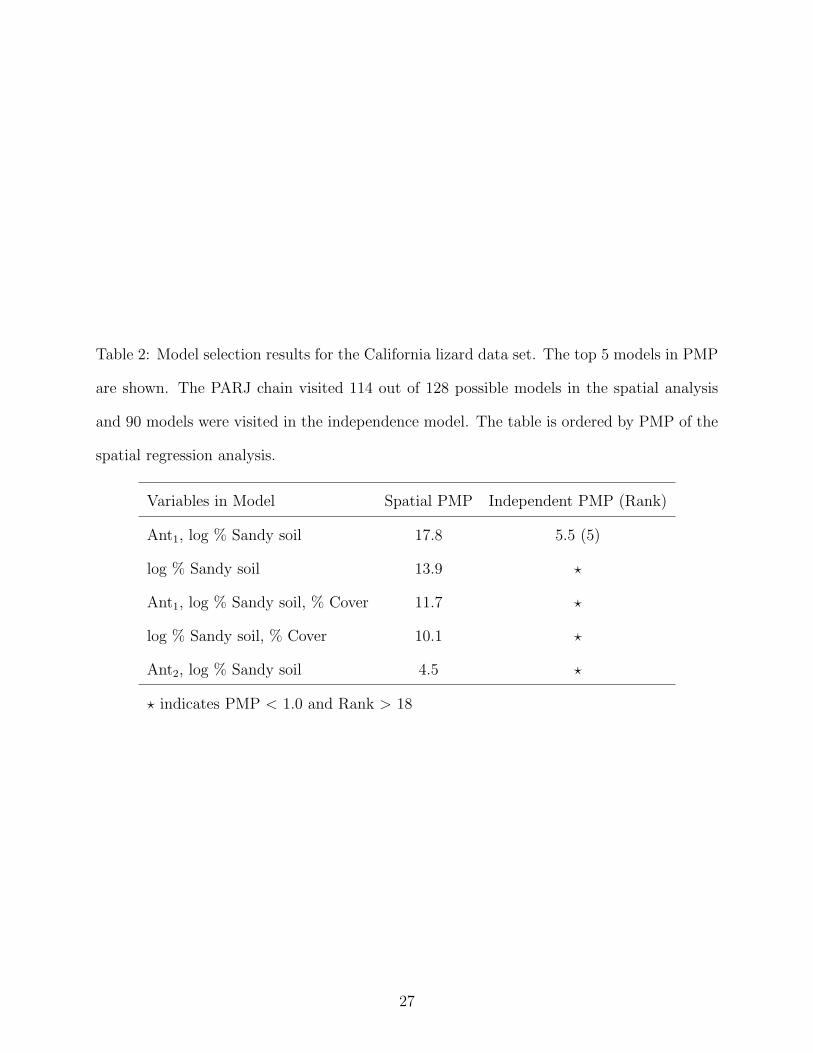
Table 2: Model selection results for the California lizard data set. The top 5 models in PMP
are shown. The PARJ chain visited 114 out of 128 possible models in the spatial analysis
and 90 models were visited in the independence model. The table is ordered by PMP of the
spatial regression analysis.
Variables in Model Spatial PMP Independent PMP (Rank)
Ant1, log % Sandy soil 17.8 5.5 (5)
log % Sandy soil 13.9 ?
Ant1, log % Sandy soil, % Cover 11.7 ?
log % Sandy soil, % Cover 10.1 ?
Ant2, log % Sandy soil 4.5 ?
? indicates PMP < 1.0 and Rank > 18
27

Table 3: Posterior inclusion probabilities (PIP) for the California lizard data. The first col-
umn of probabilities are results from a spatial analysis with nugget and anisotropy parame-
ters present in the model. The second column of probabilities resulted from an independence
model.
Environmental Covariate Spatial PIP Independent PIP
Ant1 49.5 99.8
Ant2 14.5 22.0
ln % Sandy Soil 88.4 75.3
Elevation 20.5 29.4
Bare Rock 6.1 10.7
% Cover 34.9 11.8
ln % Chaparral 7.0 76.6
28
−0.6 −0.2 0.0 0.2
01
23
4
Ant 1
0.0 0.2 0.4 0.6
01
23
4Log % Sand
−2 −1 0 1
01
23
4
Elevation
−0.2 0.0 0.2 0.4 0.6
01
23
4
% Cover
Figure 1: Marginal posterior density estimates for the top 4 PIP regression coefficients in
the lizard abundance analysis. Included are coefficients are: Ant1 (β1), log % sand (β3),
Elevation (β4), and % cover (β6). Vertical bars represent P (βj = 0) and the density curve is
a kernel estimate conditioned on βj 6= 0.
29
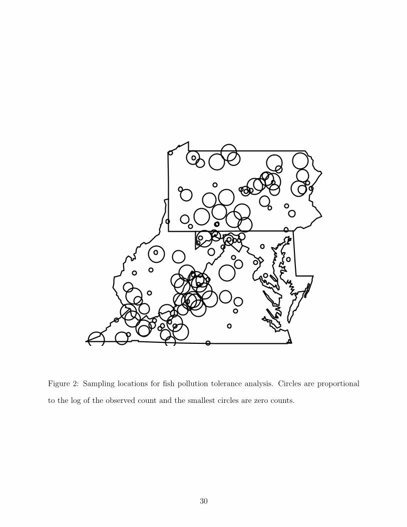
Figure 2: Sampling locations for fish pollution tolerance analysis. Circles are proportional
to the log of the observed count and the smallest circles are zero counts.
30
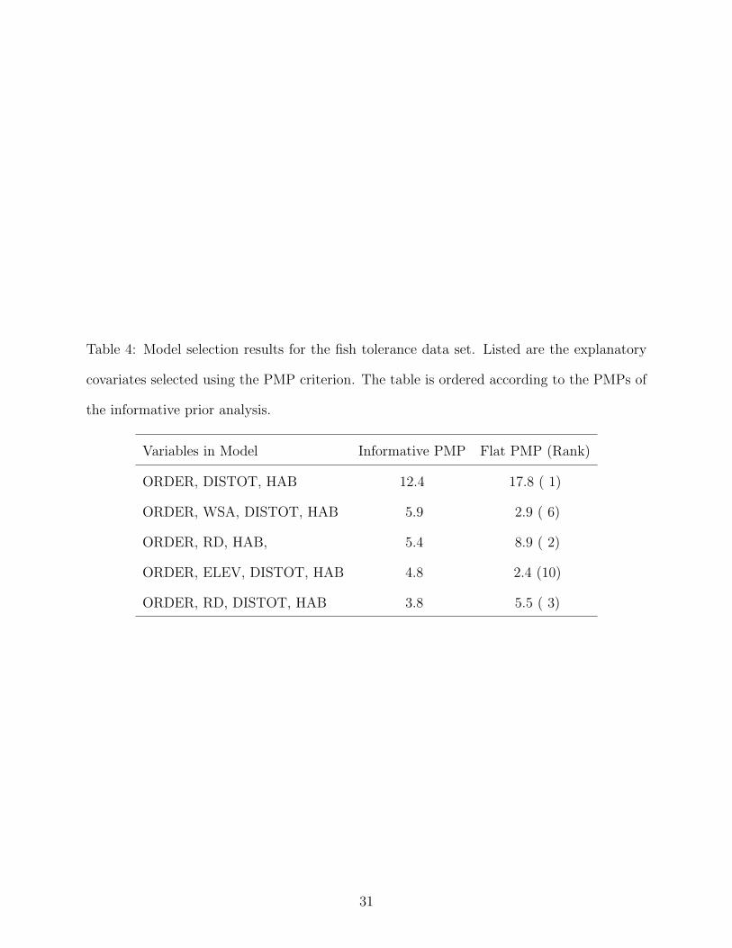
Table 4: Model selection results for the fish tolerance data set. Listed are the explanatory
covariates selected using the PMP criterion. The table is ordered according to the PMPs of
the informative prior analysis.
Variables in Model Informative PMP Flat PMP (Rank)
ORDER, DISTOT, HAB 12.4 17.8 ( 1)
ORDER, WSA, DISTOT, HAB 5.9 2.9 ( 6)
ORDER, RD, HAB, 5.4 8.9 ( 2)
ORDER, ELEV, DISTOT, HAB 4.8 2.4 (10)
ORDER, RD, DISTOT, HAB 3.8 5.5 ( 3)
31
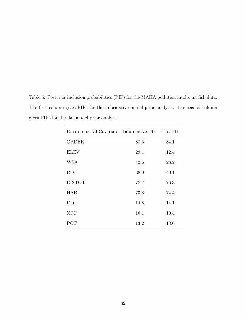
Table 5: Posterior inclusion probabilities (PIP) for the MAHA pollution intolerant fish data.
The first column gives PIPs for the informative model prior analysis. The second column
gives PIPs for the flat model prior analysis
Environmental Covariate Informative PIP Flat PIP
ORDER 88.3 84.1
ELEV 29.1 12.4
WSA 42.6 28.2
RD 38.0 40.1
DISTOT 78.7 76.3
HAB 73.8 74.4
DO 14.8 14.1
XFC 10.1 10.4
PCT 13.2 13.6
32
−1.0 0.0 1.0 2.0
0.0
0.4
0.8
1.2
Strahler Order
−1.0 0.0 1.0 2.0
0.0
0.4
0.8
1.2
Watershed Area
−2 −1 0 1
0.0
0.4
0.8
1.2
% Watershed Disturbed
−0.5 0.5 1.5
0.0
0.4
0.8
1.2
Habitat Quality Index
Figure 3: Marginal posterior density estimates for the top 4 PIP regression coefficients in
the fish abundance analysis. Included are coefficients are: stream order (β1), Watershed area
(β2), % watershed area disturbed by human use (β5), and habitat quality (β6). Vertical bars
represent P (βj = 0) and the density curve is a kernel estimate conditioned on βj 6= 0.
33
Related Documents