Bayesian Inference Applied to the Electromagnetic Inverse Problem

Bayesian Inference Applied to the Electromagnetic Inverse Problem

David M. Schmidt∗, John S. George and C.C. WoodBiophysics Group, MS-D454, Los Alamos National Laboratory, Los Alamos, NM 87545

(This paper and some figures may be found on the WEB at http://stella.lanl.gov/bi.html)

Abstract

We present a new approach to the electromagneticinverse problem that explicitly addresses the ambi-guity associated with its ill-posed character. Ratherthan calculating a single “best” solution according tosome criterion, our approach produces a large num-ber of likely solutions that both fit the data and anyprior information that is used. While the range of thedifferent likely results is representative of the ambi-guity in the inverse problem even with prior infor-mation present, features that are common across alarge number of the different solutions can be iden-tified and are associated with a high degree of prob-ability. This approach is implemented and quanti-fied within the formalism of Bayesian inference whichcombines prior information with that from measure-ment in a common framework using a single mea-sure. To demonstrate this approach, a general neuralactivation model is constructed that includes a vari-able number of extended regions of activation andcan incorporate a great deal of prior information onneural current such as information on location, orien-tation, strength and spatial smoothness. Taken to-gether, this activation model and the Bayesian in-ferential approach yield estimates of the probabilitydistributions for the number, location, and extent ofactive regions. Both simulated MEG data and datafrom a visual evoked response experiment are used todemonstrate the capabilities of this approach.

1. IntroductionUnder suitable conditions of spatial and tempo-

ral synchronization, neuronal currents are accompa-nied by electric potentials and magnetic fields thatare sufficiently large to be recorded non-invasivelyfrom the surface of the head. These are knownas the electroencephalogram (EEG) and magnetoen-cephalogram (MEG), respectively. In contrast toPET and fMRI, which measure cerebral vascularchanges secondary to changes in neuronal activity,EEG and MEG are direct physical consequences ofneuronal currents and are capable of resolving tem-poral patterns of neural activity in the millisecondrange [Hamalainen et al., 1993; Aine, 1995; Toga and

∗To whom correspondence should be addressed, Email:[email protected]

Mazziotta, 1996]. Unlike PET and fMRI, however,the problem of estimating the current distributionin the brain from surface EEG and MEG measure-ments (the so-called electromagnetic inverse prob-lem) is mathematically ill-posed; that is, it has nounique solution in the most general, unconstrainedcase [von Helmholtz, 1853; Nunez, 1981].

Existing approaches to the electromagnetic inverseproblem fall into two broad categories: (1) “few-parameter models” (i.e., those in which M N,where M is the number of parameters to be esti-mated in the model and N is the number of recordingsites); (2) and “many-parameter models” (i.e., thosein which M ≥ N). A well-known example of the “fewparameter” approach is the single- or multiple-dipolemodel [e.g., Kavanaugh et al., 1978; Scherg and vonCramon, 1986; Mosher et al., 1992], in which thecurrent is assumed to be represented by a few point-dipoles, the “order” of the model is estimated us-ing Chi-square or related statistical techniques, andthe best-fitting values of the dipole parameters (lo-cations, orientations, and magnitudes) are estimatedusing non-linear numerical minimization techniques.A well-known example of the “many-parameter” ap-proach is the “minimum-norm linear inverse” [e.g.,Hamalainen and Ilmoniemi, 1984; Dale and Sereno,1993; Hamalainen et al., 1993], in which the problemis under-determined (because M ≥ N) and a strictlymathematical criterion is used to select among themany solutions that fit the data equally well; in thecase of the minimum-norm approach the mathemat-ical criterion is the solution that minimizes the sumof squared current strengths.

In this paper we introduce a new probabilistic ap-proach to the electromagnetic inverse problem, basedon Bayesian inference [e.g., Bernardo and Smith,1994; Gelman et al., 1995]. Unlike other approachesto this problem, including other recent applicationsof Bayesian methods [Baillet and Garnero, 1997;Phillips et al., 1997], our approach does not result ina single “best” solution to the problem. Rather, weestimate a probability distribution of solutions uponwhich all subsequent inferences are based. This dis-tribution provides a means of identifying and estimat-ing the likelihood of features of current sources fromsurface measurements that explicitly emphasizes themultiple solutions that can account for any set of sur-face EEG/MEG measurements.

1


In addition to emphasizing the inherent proba-bilistic character of the electromagnetic inverse prob-lem, Bayesian methods provide a formal, quantitativemeans of incorporating additional relevant informa-tion, independent of the EEG/MEG measurementsthemselves, into the resulting probability distributionof inverse solutions. Such information might includeconstraints derived from anatomy on the likely loca-tion and/or orientation of current [Wang et al., 1992;George et al., 1995; Baillet and Garnero, 1997; Dale,1997], maximum current strength, spatial and/ortemporal smoothness of current, etc. The Bayesianapproach also provides a way to marginalize over nui-sance variables that cannot be determined or resolvedfrom the data.

We begin with an overview of the general tech-niques of Bayesian inference. Then we show howthese techniques may be applied to the EEG/MEGinverse problem and demonstrate their use in exam-ples from both simulated MEG data and MEG datafrom a visual evoked response experiment.

2. Bayesian InferenceBayesian inference (BI) is a general procedure for

constructing a (posterior) probability distribution forquantities of interest from the measurements given(prior) probability distributions for all of the uncer-tain parameters—both those that relate the quanti-ties of interest to the measurements and the quanti-ties of interest themselves. The method is conceptu-ally simple, using basic laws of probability, making itsapplication even to complicated problems relativelystraightforward. The posterior probability distribu-tion is often too complicated to be calculated ana-lytically, but can usually be adequately sampled us-ing modern computer techniques, even in problemswith many parameters. The method is outlined here,more detailed presentations can be found elsewhere[e.g., Gelman et al., 1995].

The starting point for BI is Bayes’ rule of proba-bility:

P (θ, y) = P (θ | y)P (y), (1)

where P (θ, y) is the joint probability distributionfor the quantities, θ and y, P (θ | y) is the con-ditional probability distribution of θ given y, andP (y) is the marginalized probability distribution of y;P (y) =

∑θ P (θ, y) (or P (y) =

∫P (θ, y) dθ for con-

tinuous θ). If θ represents parameters about whichwe wish to learn and y represents data bearing uponθ, then the probability of θ given y can be constructedfrom Bayes’ rule as:

P (θ | y) =P (θ, y)P (y)

=P (y | θ)P (θ)

P (y). (2)

Here P (θ) is the prior probability distribution of θwhich represents one’s knowledge of θ prior to themeasurement. This is modified by the data through

the likelihood function, P (y | θ), to produce the pos-terior probability distribution, P (θ | y). Since P (y)is independent of θ it can be considered a normalizingconstant and can be omitted from the unnormalizedposterior density:

P (θ | y) ∝ P (y | θ)P (θ). (3)

As summarized in [Gelman et al., 1995], “Thesesimple expressions encapsulate the technical core ofBayesian inference: the primary task of any spe-cific application is to develop the model P (θ, y) andperform the necessary computations to summarizeP (θ | y) in appropriate ways.”

3. Bayesian Inference Applied to theEEG/MEG Inverse Problem

3.1. Activity ModelThe methods of BI applied to the EEG/MEG in-

verse problem are demonstrated within the contextof a model for the regions of activation which is in-tended to be applicable in evoked response experi-ments. There is both theoretical and experimentalevidence that EEG and MEG recorded outside thehead arise primarily from neocortex, in particularfrom apical dendrites of pyramidal cells [e.g., Alli-son et al., 1986; Dale and Sereno, 1993; Hamalainenet al., 1993]. We therefore construct a model thatassumes a variable number of variable size corticalregions of stimulus-correlated activity in which cur-rent may be present. Specifically, an active region isassumed to consist of those locations which are iden-tified as being part of cortex and are located within asphere of some radius r centered on some location w,also in cortex. There can be any number n of theseactive regions up to some maximum nmax and the ra-dius can have any value up to some maximum, rmax.The goal is to determine the posterior probability val-ues for the set of activity parameters α = n,w, rwhich govern the number, location, and extent of ac-tive regions.

3.2. Probability Model for Activity ParametersThe first step in BI is to construct a probabil-

ity model that relates the activity parameters to themeasurements. Let the N measurements at one in-stant in time be denoted by b = b1, . . ., bN. Theconditional probability of the activity parametersgiven the observed data, P (α | b), can be expressedusing Bayes’ rule of probability as

P (α | b) ∝ P (b | α)P (α) (4)

where P (α) is the prior probability for the activityparameters and P (b | α) is the probability of thedata given a particular set of values for the activityparameters. The prior probability for the activity pa-rameters will be set by the experimenter using physi-ological information about the particular experimentbeing analyzed. Because the data do not depend onthe activity parameters directly, but rather on a given

2

D.M. Schmidt, J.S. George, C.C. Wood

current distribution j, the function, P (b | α), can notbe specified until first expanding it to include the de-pendence of the measurements on the current. Thismay be accomplished by marginalizing out the cur-rent in the joint probability of the data and currentsuch that

P (b | α) =∫P (b, j | α)Dj

=∫P (b | j,α)P (j | α)Dj (5)

where the integral is a functional integral over allcurrent distributions. The function, P (b | j,α), isthe likelihood function of the data; there is no explicitdependence upon α since j is all that is needed tocompletely specify P (b | j,α). In particular, sincemost evoked response experiments are repeated manytimes and averaged, it is assumed that the likelihoodfunction is Gaussian such that

P (b | j,α) ∝

exp

−12

N∑k,l=1

(bk − 〈ak, j〉)C−1kl (bl − 〈al, j〉)

. (6)

Here, C is the covariance matrix of the noise or back-ground in the measurements and a are the forwardfields or measurement kernel such that if there wereno noise or background the measurements would berelated to the current by the inner product:

bk = 〈ak, j〉 =∫

ak(x) · j(x) d3x. (7)

We find it convenient to use an equivalent representa-tion of Eq. 6 which has the noise covariance absorbedinto a new set of effective measurements and forwardfields, b and a, such that Eq. 6 becomes

P (b | j,α) ∝ exp

−1

2

N∑k=1

(bk − 〈ak, j〉

)2. (8)

The function P (j | α), which gives the probabilityof any current given a particular set of activity pa-rameters, needs to be constructed. Clearly the cur-rent should be zero outside of active regions. Further-more, we would like to be able to incorporate priorinformation about the limits of current strength, spa-tial variability and orientation of the current withinactive regions. For example, high-resolution currentsource density estimates suggest that net cortical cur-rents are oriented predominately perpendicular to thecortical surface [Mitzdorf, 1985]. These forms of priorinformation may be incorporated, in a manner whichsimplifies computing the marginalization over j inP (b, j | α), by using a Gaussian distribution such

that

P (j | α) ∝ |V|−12 exp

−1

2〈j,V−1

j〉

(9)

where V−1

is the inverse of the covariance opera-tor (matrix) of the current. The diagonal elements,or the variances, serve to limit the current strength,and the off-diagonal elements, which are related tothe correlation coefficients, can serve to restrict thesmoothness and orientation of the current distribu-tion. The variance at locations which are not part ofany active region for a given α is set to zero. The ex-perimenter needs to set the values of the covariancematrix, based on knowledge of the the experimentto be analyzed, using prior information about thestrength, orientation and spatial variability of cur-rent within active regions.

The full probability model for the activity param-eters is

P (α | b) ∝ P (α) |V|−12 ×∫

exp

[−1

2

N∑k=1

(bk − 〈ak, j〉

)2+ 〈j,V−1

j〉]Dj

(10)

and P (α) is set by the experimenter. The inte-gral over the current may be constructed using theeigenvalues, λθ(α), and normalized eigenvectors,ψθ(α) (θ = 1, . . . , N), of the matrix Gk,l(α) =〈ak,V al〉; all of which may be calculated usingstandard numerical techniques. Using these eigen-values and eigenvectors the formula for the posteriorprobability distribution becomes

P (α | b) ∝ P (α)×

exp[−1

2

∑k,θ,l

bkψk,θ(α)ψl,θ(α)

1 + λθ(α)bl +

∑θ

ln(1 + λθ(α))]. (11)

This formula is well-behaved and is not overly sensi-tive to very small eigenvalues. Moreover, it is rela-tively simple to compute because it only depends onthe N by N matrix, Gk,l(α).

3.3. Sampling the Posterior

The next step in BI is to use the posterior probabil-ity distribution in order to answer questions relatedto the activity parameters in terms of probability.Examples of such questions include: what is the prob-ability that there were m regions of activity? Whatare the locations for these active regions at a 95%probability level? In cases where the number of dif-ferent possible sets of activation parameters is small,one can evaluate the complete posterior distribution.Generally, however, the number of different possiblesets of activation parameters is large. In such cases

3


Fig. 1: Gray matter regions are tagged (in red) fromanatomical MRI data. These tagged voxels consti-tute the anatomical model used to implement thecortical location and orientation prior information.

the method of Markov Chain Monte Carlo (MCMC)can be used to generate a sample of sets of activ-ity parameters which are distributed according to theposterior distribution. This is known as sampling theposterior, the techniques for which are described indetail elsewhere [e.g., Gelman et al., 1995].

4. ExamplesWhile the methods just described apply to mod-

els for both EEG and MEG data, in the remainderof this paper we will use MEG data to illustrate theproperties of the approach. Both simulated and em-pirical MEG data for a Neuromag-122 whole-headsystem were used. The physical setup of the actualMEG experiment was used to determine the locationof the subject’s head relative to the sensors in thesimulated data examples. In addition, an anatomicalMRI data set acquired from the subject in the MEGexperiment was used to determine the location of cor-tex (actually gray matter) using MRIVIEW (Fig 1),a software tool developed in our laboratory [Rankenand George, 1993]. About 50,000 voxels were taggedand the normal directions for each of these voxels wasthen determined by examining the curvature of thelocal tagged region.

A spherically symmetric conductivity model wasused to calculate the expected measurements given acurrent source both for the simulated data and in thelikelihood calculations [Sarvas, 1987]. The same priorassumptions were used with the simulated data sets,with only minor changes for the real data example.Specifically the prior probability function P (α) wasuniform so that each set of activation parameters hadthe same prior probability. The number of activeregions was allowed to range from 0 to 8 and theradius of any region of activity was allowed to rangefrom 0 to 10 mm.

The covariance matrix was factored such that

βγV(i, j) = σ(i)σ(j)ρ(i− j) βγΩ(i, j) (12)

Fig. 2: Maximum intensity projection of the locationand extent (in black) of the active region used togenerate simulated MEG data for Example 1.

where β and γ are orientation indices, i and j arelocation indices, σ(i) is the standard deviation atlocation i, ρ(i− j) is the spatial correlation function,and βγΩ(i, j) is the orientation covariance. The cor-relation function was chosen to be a Gaussian withzero mean and 7 mm standard deviation which im-poses spatial smoothness on scales of about 7 mmor less. Because of this prior information concern-ing spatial correlation, the continuous current distri-butions and integrals of the previous section may bewell-approximated by discrete distributions and sumsover the volume elements (voxels) that were taggedfrom the anatomical MRI data. For example, in eval-uating the posterior probability value using Eq. 11the matrix G is calculated in the following examplesby approximating the continuous integral with a sumover tagged voxels. This is a good approximation be-cause the covariance operator has a correlation lengthof 7 mm which is larger than the voxel dimensions of2 mm on a side.

To complete the specification of the covariance op-erator, a value of 2 nAm was used for σ(i) at alllocations in active regions and 0 nAm elsewhere. Theorientation covariance was chosen such that therewas no correlation between the orientations at differ-ent locations and the orientation distribution at anygiven location was symmetric with respect to the di-rection normal to the cortical surface at that locationand had a mean equal to the cortical norm directionand a standard deviation of 30. Unlike other recentimplementations of cortical constraints in distributedinverse solutions [e.g., Dale and Sereno, 1993; Bailletand Garnero, 1997], this procedure results in a distri-bution of orientations around the perpendicular, nota fixed normal orientation.

Finally, the same noise was added to all simulateddata sets, which was Normal with a standard de-viation of 10 fT. The values used here in the priorprobability distribution are meant to be an exampleof what one might choose for a MEG analysis andshould be chosen for each particular MEG data set.

4.1. Example 1

The location and extent of the active region used togenerate the simulated MEG data is shown in Fig. 2.The bounding radius of the active region was 5 mm

4


a)b)

Fig. 3: The simulated data used in Example 1, a) asa function of channel number, b) as a field pattern asviewed from a top projection.

and the current dipole strength at each voxel was2 nAm oriented in the cortical normal direction. Aplot of the simulated data and its field pattern isshown in Fig. 3. Ten thousand samples were drawnfrom the posterior distribution using a MCMC algo-rithm. A plot of the posterior probability for eachof the samples is shown in Fig. 4. It took about 600samples to progress from the starting point whichhad a low probability to one that had a high prob-ability and was therefore representative of the pos-terior distribution. Only the final 9,000 samples, afew of which are shown in Fig. 5, were used in mak-ing probabilistic inferences as discussed below. Allof the samples shown in Fig. 5 are among the 95%most probable and therefore fit both the data and theprior expectations quite well. Any of these could haveproduced the given MEG data, yet there are clearlyvast differences among the samples. The number ofactive regions ranges from 1 to 5, the sizes of theregions vary greatly and the locations of the activeregions vary nearly across the entire tagged region ofthe brain (when considering all 9,000 samples). Thisvariability is a representation of the degree of the am-biguity of the inverse problem for these MEG data,even with the prior information present.

Despite the degree of variability among the sam-ples in Fig. 5 a property common to all is apparent;namely an active region in the dorsal, lateral regionof the right hemisphere. A feature, such as this, com-mon to all or most of the samples, is associated witha high degree of probability. This probability canbe quantified because the MCMC samples are dis-tributed according to the posterior probability distri-bution. The smallest set of voxels which contains thecenter of the active region in the dorsal, lateral regionin 95% of the samples was identified and is shown inFig. 6. This region, which contains a center of ac-tivity with a probability of 95%, in fact encompassesthe region of activity which was used to produce thesimulated data set (Fig. 2). Although it is nice tosee this agreement, it is not sufficient to justify thisor any MEG inverse method based solely on whetherit produces results consistent with the true active re-

Fig. 4: The posterior probability of the 10,000 sam-ples drawn from the posterior probability distributionof Example 1. This figure shows the progression ofthe MCMC sampling algorithm.

Fig. 5: A few of the 9,000 samples drawn from theposterior probability distribution of Example 1. Eachpanel shows 3 views of the maximum intensity pro-jection of active regions from a single sample. All ofthese samples could have produced the same MEGdata set.

gions because any of the sets of active regions shownin Fig. 5 could have also been used to generate thesame MEG data. Any robust and highly probable re-sult or inference therefore should be consistent withthe wide range of possible sets of active regions, asis the result in Fig. 6 by construction. This is a veryimportant feature of BI which is necessarily missingfrom any other analysis method which only considersjust one possible result, even if it happens to be the

5


Fig. 6: Maximum intensity projections of the locationand extent of a region containing a center of activityat a 95% probability level in Example 1.

most likely result within a given model.In addition to the information about the locations

of probable regions of activity, the Bayesian approachcombined with this activity model also provides prob-abilistic information about the number and size of ac-tive regions. The posterior distribution for the num-ber of active regions was constructed by histogram-ing the number of regions across the MCMC sam-ples. This histogram is shown in Fig. 7a. One ac-tive region is the most probable; however, two activeregions are quite likely as well. Although the loca-tion of one active region was identified in the lastparagraph, the location of a second could not be welllocalized because it occurred in a wide range of lo-cations across the MCMC samples. Assuming therewas only one active region present, we can obtaininformation about its size by histograming the sizeof active regions in the MCMC samples that hadonly one region present. This histogram is shownin Fig. 7b and represents the posterior probabilityfor the bounding radius of the active region, assum-ing that there was only one region active. Regionssmaller than 2 mm and larger than 8 mm in radius arevery unlikely whereas regions that are around 5 mmin radius are likely. The size of the region used to pro-duce the simulated data was 5 mm. We believe thatmuch of the information on size derives from priorinformation about location, orientation and strengthof neural current.

Other inferences could be drawn using the MCMCsamples in a similar manner. For example, one couldconstruct the probability for the size of the activeregion, assuming there was one centered within the95% probability region shown in Fig. 6, rather thanassuming there was only one active region presentthroughout the entire head as was done above.

4.2. Example 2

A second simulated data set was generated usingthe three active regions of different sizes shown inFig. 8. The most anterior region is centered at thesame location as the region in the first example ex-cept for this case it has a bounding radius of 8 mm.A current dipole strength of 2 nAm oriented normalto cortex was used at each voxel within this bound-ing sphere. The nearby, more posterior region had

a)

b)

Fig. 7: The posterior probability for a) the numberof active regions present in Example 1 and b) theradius of the sphere bounding activity in Example 1,assuming there was only one active region present..

Fig. 8: Maximum intensity projections of the locationand extent of the active regions used to generate thesimulated MEG data for Example 2.

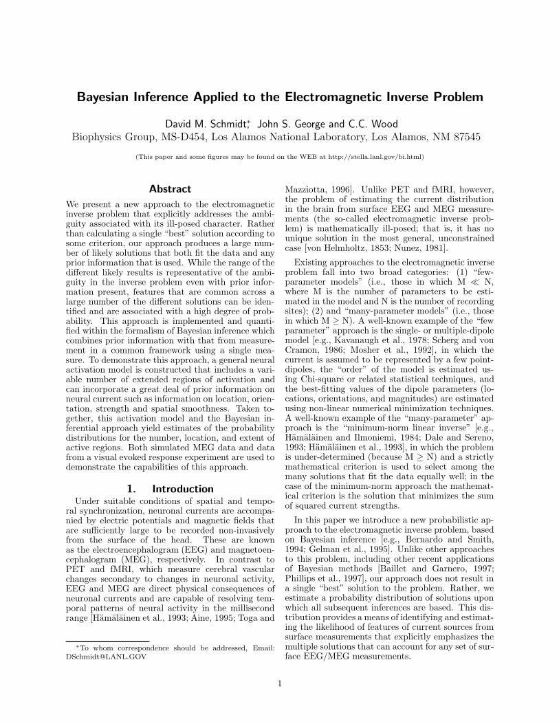
a bounding radius of 5 mm and a current dipolestrength of 2.5 nAm was used. The most posteriorregion had a 3 mm bounding radius and a currentdipole strength of 1.5 nAm. The same noise and priorassumptions where used here as for the first example.Figure 9 shows a plot of the resulting simulated dataand the field pattern.

Ten thousand samples were drawn from the poste-rior of which the final 8,000 were used to make prob-abilistic inferences. Just as in the first example weexpect there to be many different locations where ac-tivity may be found in these samples. Since we areinterested in those locations which contain activityin most of the samples it is useful to make a his-togram of the locations of the centers of active regionsacross the 8,000 samples. This histogram is shown inFig. 10. It is relatively simple to determine those re-

6


a) b)

Fig. 9: The simulated data of Example 2, a) as afunction of channel number and b) as a field patternin a top projection view.

Fig. 10: Maximum intensity projections of the his-togram of centers of active regions across the MCMCsamples in Example 2, shown on top of surface ren-derings of cortex. The darker the shade of a regionthe larger the value of the histogram at that location.

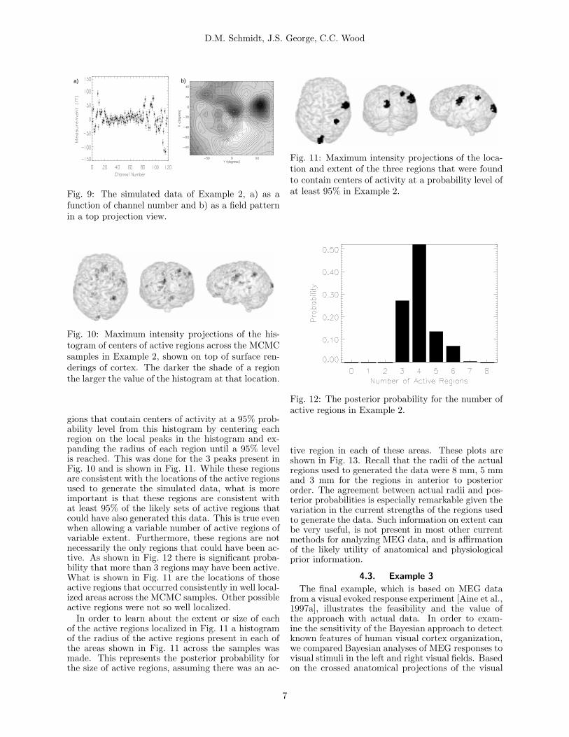
gions that contain centers of activity at a 95% prob-ability level from this histogram by centering eachregion on the local peaks in the histogram and ex-panding the radius of each region until a 95% levelis reached. This was done for the 3 peaks present inFig. 10 and is shown in Fig. 11. While these regionsare consistent with the locations of the active regionsused to generate the simulated data, what is moreimportant is that these regions are consistent withat least 95% of the likely sets of active regions thatcould have also generated this data. This is true evenwhen allowing a variable number of active regions ofvariable extent. Furthermore, these regions are notnecessarily the only regions that could have been ac-tive. As shown in Fig. 12 there is significant proba-bility that more than 3 regions may have been active.What is shown in Fig. 11 are the locations of thoseactive regions that occurred consistently in well local-ized areas across the MCMC samples. Other possibleactive regions were not so well localized.

In order to learn about the extent or size of eachof the active regions localized in Fig. 11 a histogramof the radius of the active regions present in each ofthe areas shown in Fig. 11 across the samples wasmade. This represents the posterior probability forthe size of active regions, assuming there was an ac-

Fig. 11: Maximum intensity projections of the loca-tion and extent of the three regions that were foundto contain centers of activity at a probability level ofat least 95% in Example 2.

Fig. 12: The posterior probability for the number ofactive regions in Example 2.

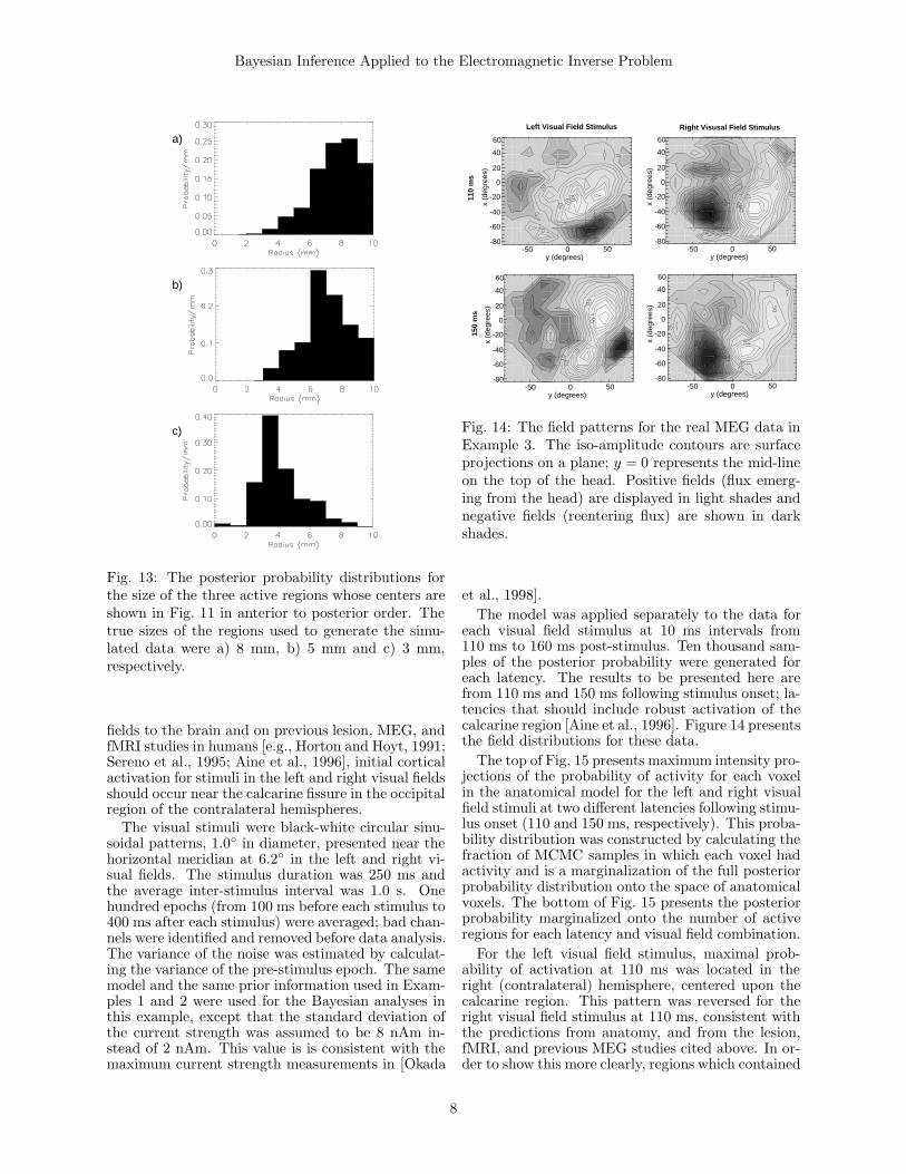
tive region in each of these areas. These plots areshown in Fig. 13. Recall that the radii of the actualregions used to generated the data were 8 mm, 5 mmand 3 mm for the regions in anterior to posteriororder. The agreement between actual radii and pos-terior probabilities is especially remarkable given thevariation in the current strengths of the regions usedto generate the data. Such information on extent canbe very useful, is not present in most other currentmethods for analyzing MEG data, and is affirmationof the likely utility of anatomical and physiologicalprior information.

4.3. Example 3

The final example, which is based on MEG datafrom a visual evoked response experiment [Aine et al.,1997a], illustrates the feasibility and the value ofthe approach with actual data. In order to exam-ine the sensitivity of the Bayesian approach to detectknown features of human visual cortex organization,we compared Bayesian analyses of MEG responses tovisual stimuli in the left and right visual fields. Basedon the crossed anatomical projections of the visual

7


a)

b)

c)

Fig. 13: The posterior probability distributions forthe size of the three active regions whose centers areshown in Fig. 11 in anterior to posterior order. Thetrue sizes of the regions used to generate the simu-lated data were a) 8 mm, b) 5 mm and c) 3 mm,respectively.

fields to the brain and on previous lesion, MEG, andfMRI studies in humans [e.g., Horton and Hoyt, 1991;Sereno et al., 1995; Aine et al., 1996], initial corticalactivation for stimuli in the left and right visual fieldsshould occur near the calcarine fissure in the occipitalregion of the contralateral hemispheres.

The visual stimuli were black-white circular sinu-soidal patterns, 1.0 in diameter, presented near thehorizontal meridian at 6.2 in the left and right vi-sual fields. The stimulus duration was 250 ms andthe average inter-stimulus interval was 1.0 s. Onehundred epochs (from 100 ms before each stimulus to400 ms after each stimulus) were averaged; bad chan-nels were identified and removed before data analysis.The variance of the noise was estimated by calculat-ing the variance of the pre-stimulus epoch. The samemodel and the same prior information used in Exam-ples 1 and 2 were used for the Bayesian analyses inthis example, except that the standard deviation ofthe current strength was assumed to be 8 nAm in-stead of 2 nAm. This value is is consistent with themaximum current strength measurements in [Okada

-50 0 50y (degrees)

60

40

20

0

-20

-40

-60

-80

x (d

egre

es)

-50 0 50y (degrees)

60

40

20

0

-20

-40

-60

-80

x (d

egre

es)

-50 0 50y (degrees)

60

40

20

0

-20

-40

-60

-80

x (d

egre

es)

-50 0 50y (degrees)

60

40

20

0

-20

-40

-60

-80

x (d

egre

es)

Left Visual Field Stimulus Right Visusal Field Stimulus

110

ms

150

ms

Fig. 14: The field patterns for the real MEG data inExample 3. The iso-amplitude contours are surfaceprojections on a plane; y = 0 represents the mid-lineon the top of the head. Positive fields (flux emerg-ing from the head) are displayed in light shades andnegative fields (reentering flux) are shown in darkshades.

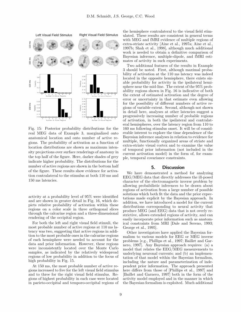
et al., 1998].The model was applied separately to the data for

each visual field stimulus at 10 ms intervals from110 ms to 160 ms post-stimulus. Ten thousand sam-ples of the posterior probability were generated foreach latency. The results to be presented here arefrom 110 ms and 150 ms following stimulus onset; la-tencies that should include robust activation of thecalcarine region [Aine et al., 1996]. Figure 14 presentsthe field distributions for these data.

The top of Fig. 15 presents maximum intensity pro-jections of the probability of activity for each voxelin the anatomical model for the left and right visualfield stimuli at two different latencies following stimu-lus onset (110 and 150 ms, respectively). This proba-bility distribution was constructed by calculating thefraction of MCMC samples in which each voxel hadactivity and is a marginalization of the full posteriorprobability distribution onto the space of anatomicalvoxels. The bottom of Fig. 15 presents the posteriorprobability marginalized onto the number of activeregions for each latency and visual field combination.

For the left visual field stimulus, maximal prob-ability of activation at 110 ms was located in theright (contralateral) hemisphere, centered upon thecalcarine region. This pattern was reversed for theright visual field stimulus at 110 ms, consistent withthe predictions from anatomy, and from the lesion,fMRI, and previous MEG studies cited above. In or-der to show this more clearly, regions which contained

8


Left Visual Field Stimulus Right Visual Field Stimulus

110

ms

150

ms

150

ms

110

ms

Fig. 15: Posterior probability distributions for thereal MEG data of Example 3, marginalized ontoanatomical location and onto number of active re-gions. The probability of activation as a function oflocation distributions are shown as maximum inten-sity projections over surface renderings of anatomy inthe top half of the figure. Here, darker shades of greyindicate higher probability. The distributions for thenumber of active regions are shown in the bottom halfof the figure. These results show evidence for activa-tion contralateral to the stimulus at both 110 ms and150 ms latencies.

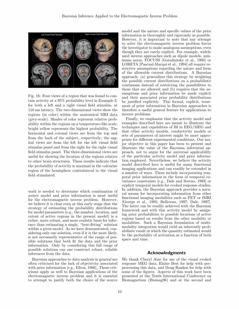
activity at a probability level of 95% were identifiedand are shown in greater detail in Fig. 16, which de-picts relative probability of activation within theseregions on a color scale in three orthogonal slicesthrough the calcarine region and a three-dimensionalrendering of the occipital region.

For both the left and right visual field stimuli, themost probable number of active regions at 110 ms la-tency was two, suggesting that active regions in addi-tion to the most probable ones in the calcarine regionsof each hemisphere were needed to account for thedata and prior information. However, these regionswere inconsistently located over the Monte Carlosamples, as indicated by the relatively widespreadregions of low probability in addition to the focus ofhigh probability in Fig. 15.

At 150 ms, the most probable number of active re-gions increased to five for the left visual field stimulusand to three for the right visual field stimulus. Re-gions of highest probability in each case were locatedin parieto-occipital and temporo-occipital regions of

the hemisphere contralateral to the visual field stim-ulated. These results are consistent in general termswith MEG and fMRI evidence of multiple regions ofextra-striate activity [Aine et al., 1997a; Aine et al.,1997b; Shah et al., 1998], although much additionalwork is needed to obtain a definitive comparison ofBayesian inference, multiple-dipole, and fMRI esti-mates of activity in such experiments.

Two additional features of the results in Example3 should be noted. First, although maximal proba-bility of activation at the 110 ms latency was indeedlocated in the opposite hemisphere, there exists siz-able probability for activity in the ipsilateral hemi-sphere near the mid-line. The extent of the 95% prob-ability regions shown in Fig. 16 is indicative of boththe extent of estimated activation and the degree oferror or uncertainty in that estimate even allowingfor the possibility of different numbers of active re-gions of variable extent. Second, although not shownin detail here, analyses at other latencies suggest aprogressively increasing number of probable regionsof activation, in both the ipsilateral and contralat-eral hemispheres, over the latency region from 110 to160 ms following stimulus onset. It will be of consid-erable interest to explore the time dependence of theBayesian inference analyses in relation to evidence formultiple, functionally organized areas of striate andextra-striate visual cortex and to examine the valueof temporal prior information (not included in thecurrent activation model) in the form of, for exam-ple, temporal covariance constraints.

5. DiscussionWe have demonstrated a method for analyzing

EEG/MEG data that directly addresses the ill-posedcharacter of the electromagnetic inverse problem byallowing probabilistic inferences to be drawn aboutregions of activation from a large number of possiblesolutions which both fit the data and the prior expec-tations made explicit by the Bayesian approach. Inaddition, we have introduced a model for the currentdistributions corresponding to neural activity thatproduce MEG (and EEG) data that is not overly re-strictive, allows extended regions of activity, and caneasily incorporate prior information such as anatom-ical constraints from MRI [Dale and Sereno, 1993;George et al., 1995].

Other investigators have applied the Bayesian for-malism to various models for EEG or MEG inverseproblems [e.g., Phillips et al., 1997; Baillet and Gar-nero, 1997]. Any Bayesian approach requires: (a) amodel that relates the EEG/MEG measurements tounderlying neuronal currents; and (b) an implemen-tation of that model within the Bayesian formalism,including the nature and parameterization of inde-pendent prior information. The approach presentedhere differs from those of [Phillips et al., 1997] and[Baillet and Garnero, 1997] both in the form of theactivity model employed and in the manner in whichthe Bayesian formalism is exploited. Much additional

9


Left Visual Field Stimulus Right Visual Field Stimulus

Fig. 16: Four views of a region that was found to con-tain activity at a 95% probability level in Example 3,for both a left and a right visual field stimulus, at110 ms latency. The two-dimensional views show theregions (in color) within the anatomical MRI data(grey-scale). Shades of color represent relative prob-ability within the regions on a temperature-like scale;bright yellow represents the highest probability. Thehorizontal and coronal views are from the top andfrom the back of the subject, respectively; the sag-ital views are from the left for the left visual fieldstimulus panel and from the right for the right visualfield stimulus panel. The three-dimensional views areuseful for showing the location of the regions relativeto other brain structures. These results indicate thatthe probability of activity is maximal in the calcarineregion of the hemisphere contralateral to the visualfield stimulated.

work is needed to determine which combination ofsource model and prior information is most usefulfor the electromagnetic inverse problem. However,we believe it is clear even at this early stage that thestrategy of estimating the probability distributionsfor model parameters (e.g., the number, location, andextent of active regions in the present model) is aricher, more robust, and more realistic basis for infer-ence than estimating a single, “best-fitting” solutionwithin a given model. As we have demonstrated, con-sidering only one solution, even if it is the most likely,is not necessarily representative of the range of pos-sible solutions that both fit the data and the priorinformation. Only by considering this full range ofpossible solutions can one construct robust, reliableinferences from the data.

Bayesian approaches to data analysis in general areoften criticized for the lack of objectivity associatedwith prior information [e.g., Efron, 1986]. Those crit-icisms apply as well to Bayesian applications of theelectromagnetic inverse problem and it is essentialto attempt to justify both the choice of the source

model and the nature and specific values of the priorinformation as thoroughly and rigorously as possible.However, it is important to note that any attemptto solve the electromagnetic inverse problem forcesthe investigator to make analogous assumptions, eventhough they are rarely explicit. For example, widelyused inverse approaches such as dipole models, min-imum norm, FOCUSS [Gorodnitsky et al., 1995] orLORETA [Pascual-Marqui et al., 1994] all require re-strictive assumptions regarding the nature and formof the allowable current distributions. A Bayesianapproach: (a) generalizes this strategy by weightingthe possible current distributions on a probabilisticcontinuum instead of restricting the possibilities tothose that are allowed; and (b) requires that the as-sumptions and prior information be made explicitand their associated prior probability distributionsbe justified explicitly. This formal, explicit, treat-ment of prior information in Bayesian approaches istherefore a useful general feature for applications toinverse problems.

Finally, we emphasize that the activity model andexamples described here are meant to illustrate thetechniques and capabilities of BI in EEG/MEG andthat other activity models, conductivity models orsets of parameters of interest might be more appro-priate for different experimental conditions. Our ma-jor objective in this paper has been to present andillustrate the value of the Bayesian inferential ap-proach, not to argue for the universal applicabilityof the particular activity model and prior informa-tion employed. Nevertheless, we believe the activitymodel described here is useful for many functionalimaging applications and can readily be extended ina number of ways. These include incorporating tem-poral prior information in the form of temporal co-variance constraints [e.g., Dale and Sereno, 1993] orexplicit temporal models for evoked response studies.In addition, the Bayesian approach provides a natu-ral means for incorporating information from otherfunctional imaging modalities such as PET or fMRI[George et al., 1995; Belliveau, 1997; Dale, 1997].The latter can be readily achieved with the Bayesianframework and with this activity model by assign-ing prior probabilities to possible locations of activeregions based on results from the other modality ormodalities. Such a Bayesian formulation of multi-modality integration would yield an inherently prob-abilistic result in which the quantity estimated wouldbe the probability of activation as a function of bothspace and time.

Acknowledgments

We thank Cheryl Aine for use of the visual evokedresponse MEG data, Elaine Best for help with pre-processing this data, and Doug Ranken for help withsome of the figures. Aspects of this work have beenpresented at the Tenth International Conference onBiomagnetism (Biomag96) and at the second and

10


third international conferences on Functional Map-ping of the Human Brain. Supported by: NIH GrantsEY0861003 and DA/MH09972, the Los Alamos Na-tional Laboratory and the United States Departmentof Energy.

References

Aine CJ (1995): A conceptual overview and cri-tique of functional neuroimaging techniques inhumans: I. MRI/fMRI and PET. Critical Re-views in Neurobiology, 9:229–309.

Aine C, Supek S, George J, Ranken D, Lewine J,Sanders J, Best E, Tiee W, Flynn E, Wood C(1996): Retinotopic organization of human vi-sual cortex: Departures from the classical model.Cerebral Cortex, 6:354–361.

Aine C, Chen HW, Ranken D, Mosher J, Best E,George J, Lewine J, Paulson K (1997a): An ex-amination of chromatic/achromatic stimuli pre-sented to central/peripheral visual fields: AnMEG study. Neuroimage, 5:153.

Aine C, Schlitt H, Shah J, Ranken D, KrauseB, George J, Muller-Gartner HW (1997b):MEG/fMRI differentiates betweeen ven-tral/dorsal processing streams. Soc. Neurosci.,23:1312.

Allison T, Wood C, McCarthy G (1986). The cen-tral nervous system. In: Donchin E, PorgesS, Coles M (eds): Psychophysiology: Systems,Processes and Applications: A Handbook. NewYork: Guilford Press, pp. 5–25.

Baillet S, Garnero L (1997): A bayesian approachto introducing anatomo-functional priors in theEEG/MEG inverse problem. IEEE Trans.Biomed. Eng., 44(5):374–385.

Belliveau J (1997): Dynamic human brain mappingusing combined fMRI, EEG and MEG. In: Apresentation to the symposium on approachesto cognitive neuroscience by means of functionalbrain imaging, Caen, France.

Bernardo J, Smith A (1994): Bayesian Theory. NewYork: Wiley.

Dale AM, Sereno MI (1993): Improved localizationof cortical activity by combining EEG and MEGwith MRI cortical surface reconstruction: A lin-ear approach. J. Cognitive Neurosci., 5:162–176.

Dale A (1997): Strategies and limitations in integrat-ing brain imaging and electromagnetic record-ing. Soc. Neurosci. Abst., 23:1.

Efron B (1986): Why isn’t everyone a Bayesian?American Statistician, 40(1):1–5; commentary5–11.

Gelman A, Carlin JB, Stern HS, Rubin DB (1995):Bayesian Data Analysis. London: Chapman &Hall.

George J, Aine C, Mosher J, Schmidt D, Ranken D,Schlitt H, Wood C, Lewine J, Sanders J, Bel-liveau J (1995): Mapping function in the humanbrain with MEG, anatomical MRI, and func-tional MRI. J. Clin. Neurophys., 12:406–431.

Gorodnitsky I, George J, Rao B (1995): Neuromag-netic source imaging with FOCUSS: a recursiveweighted minimum norm algorithm. Electroen-ceph. Clin. Neurophysiol., 95:231–251.

Hamalainen M, Ilmoniemi R (1984). Interpretingmeasured magnetic fields of the brain: estimatesof current distributions. Technical Report TKK-F-A559, Helsinki University of Technology, Fin-land.

Hamalainen M, Hari R, Ilmoniemi RJ,Knuutila J, Lounasmaa OV (1993):Magnetoencephalography—theory, instru-mentation, and applications to noninvasivestudies of the working human brain. Rev. Mod.Phys., 65(2):413–497.

Horton J, Hoyt W (1991): The representation of thevisual field in human striate cortex. Proc. Roy.Soc. London, 132:348–361.

Kavanaugh R, Darcey T, Lehmanh D, FenderD (1978): Evaluation of methods for three-dimensional localization of electrical sources inthe human brain. IEEE Trans. Biomed. Eng.,25:421–429.

Mitzdorf U (1985): Current source-density methodand application in cat cerebral-cortex : Inves-tigation of evoked-potentials and EEG phenom-ena. Physiological Reviews, 65(1):37–100.

Mosher JC, Lewis PS, Leahy RM (1992): Multipledipole modeling and localization from spatio-temporal MEG data. IEEE Trans. Biomed.Eng., 39(6):541–557.

Nunez P (1981): Electrical fields of the brain: neuro-physics of the EEG. Oxford: Oxford UniversityPress.

Okada YC, Papuashvili N, Xu C (1998): Maximumcurrent dipole moment density as an importantphysiological constraint in MEG inverse solu-tions. In: Proceedings of the Tenth Interna-tional Conference on Biomagnetism (in press).

11


Pascual-Marqui RD, Michel CM, Lehmann D (1994):Low resolution electromagnetic tomography: Anew method for localizing electrical activity ofthe brain. Int. J. Psychophysiology, 18(1):49–65.

Phillips JW, Leahy RM, Mosher JC (1997): MEG-based imaging of focal neuronal current sources.IEEE Trans. Med. Imag., 16(3):338–348.

Ranken DM, George JS (1993): MRIVIEW: An in-teractive computational tool for investigation ofbrain structure and function. In: Visualization’93, pp. 324–331. IEEE Computer Society.

Sarvas J (1987): Basic mathematical and electromag-netic concepts of the biomagnetic inverse prob-lem. Phys. Med. Biol., 32(1):11–22.

Scherg M, von Cramon D (1986): Evoked dipolesource potentials of the human auditory cortex.Electroenceph. Clin. Neurophysiol., 65:344–360.

Sereno M, Dale A, Reppas J, Kwong K, Belliveau J,Brady T, Rosen B, Tootell R (1995): Bordersof multiple visual areas in human revealed byfunctional magnetic resonance imaging. Science,268:889–893.

Shah N, Aine C, Schlitt H, Krause B, Ranken D,George J, Muller-Gartner HW (1998). Activa-tion of the ventral stream in humans: An fMRIstudy. In: Gulyas B, Muller-Gartner HW (eds):Positron Emission Tomography: A Critical As-sessment of Recent Trends (in press). Dordrecht:Kluwer Academic Publishers.

Toga AW, Mazziotta JC (1996): Brain Mapping:The Methods. New York: Academic Press.

von Helmholtz H (1853): Ueber einige gesetzeder vertheilung elektrischer strome in korper-lichen leitern, mit anwendung auf die thierisch-elektrischen versuche. Ann. Phys. Chem,89:211–233 and 353–377.

Wang J, Williamson S, Kaufman L (1992): Magneticsource images determined by a lead-field analy-sis: the unique minimum-norm. IEEE Trans.Biomed. Eng., 39(7):665–675.

12

Bayesian Inference Applied to the Electromagnetic Inverse Problem

Documents