Bayesian estimation of soil parameters from radar backscatter data

d“

Bayesian estimation of soil parametersfrom radar backscatter data

Ziad S. HaddadPascale Dubois

Jet Propulsion Laboratory, California Institute of Technology

Abstract

Given measurements ml, 7TLZ,. . . . nz~ representing radar cross-sections of a given resolutionelement at different polarizations and/or different frequency bands, we consider the problemof making an “optimal’ ) estimate of the actual dielectric constant c and the r,m.s. surfaceheight h that gave rise to the particular {ntj ) observed. TO obtain such an algorithm, westart with a data catalogue consisting of careful measurements of the soil parameters c andh, and the corresponding remote sensing data {mj }. We also assume that we have used thisdata to write down, for each j, an average formula which associates an approximate value ofmj to a given pair (E, h). Instead of deterministica]]y inverting these average formulas, wepropose to use the data catalogue more fully and quantify the spread of the measurementsabout the average formula, then incorporate this information into the inversion algorithm.q’his paper describes how we accomplish this using a Elayesian approach. In fact, our methodallows us to

1)

2)

3)

4)

make an optimal estimate of E and h

place a quantitatively honest error bar oil each estimate, as a function of the actualvalues of the remote sensing measurements

.fine-tune the inital formulas expressing the dependence of the remote sensing data onthe soil parameters

take into account as many (or as few) remote sensing measurements as we like inmaking our estimates of c and h, in each case producing error bars to quantify thebenefits of using a particular combination of measurements.

1 Introduction

,

4

Several investigators ([1], [5],[7],[8], [9], [10], [1 1],[12], [14], [15]) have studied the use of remotesensing methods to estimate the physical parameters of natural surfaces, namely the soilmoisture content and the r.m.s. surface roughness. Because the laws of scattering from ran-domly rough natural surfaces are quite complicated, especially at microwave frequencies,empirical models have often been used to help express the observed remote sensing measure-nients as a function of the surface parameters. A typical approach, adopted in ([10]), is tostart with a ‘lraining set)) consisting of a catalogue of carefully collected data: in the caseof [10], this catalogue consists of L-, C- and X-band polarimetric radar backscattering mea-surements for various bare soil surfaces, along wit h laser-profiler and dielectric-probe n~ea-surements of the corresponding r,m, s. surface height and dielectric constant values, Guidedby the physics that govern electromagnetic scattering, and using the data at hand, a modelrelating the radar backscatter to the surface parameters can be established. Of course, themodel wiIl not agree exactly with the data in every instance. Reasons for mismatches includemeasurement e,rror, the non-uniformity of the background power distribution, and the inho-mogeneit y of the surface within a given resolution element or from one element to the next.Still, if the model is regarded as providing an approximate formula that is correct on average,one way to proceed is to disregard the data catalogue from this point on: given a particularradar measurement, a deterministic method can be used to invert the approximate modeland retrieve the corresponding surface parameters, The accuracy of the retrieved parameterswould naturally depend on the inversion method used, and would be difficult to quantify.

Another approach, that can potentially make fuller use of the data catalogue, is to modelnot only the approximate dependence of the radar backscatter on the surface parameters, butalso the spread of the actual data about the approximate model. Indeed, the approximatemodel can be more or less accurate over certain intervals, Using this information about itsaccuracy, and how it depends on the values of the surface parameters, as evidenced” by thecarefully collected data, can only help in the inversion problem. In fact,

1)

2)

3)

. .

a Bayesian approach can indeed use this information to produce an optimal algo-rithm, i.e. an algorithm which, among all possible algorithms, and on average, makesthe smallest error in its estimates of the surface parameters.

Moreover, such an approach can quantify the accuracy of its estimates, depending,naturally, on the values of the measured radar backscatter in every case.

It also turns out that the approach allows one to fine-tune the initial approximatemodel to better fit the data.

2

.,, ..

.

4), Finally, the approach does not restrict one to a prespecified number of input measure-ments: indeed, it can use any combination of inputs to produce an estimateof the surface parameters that is based on these inputs. Moreover, it can quantify theuncertainty of these estimates. This is important because it provides a natural meansof evaluating the usefulness of using one or another combination of measurements toestimate one or another surface parameter.

Section 2 summarizes the mathematics underlying the 13ayesian approach in the case athand. At the heart of this approach is the problem of modeling the spread of the data in the“training set” about the approximate model. This is described in section 3. Finally, section4 discusses the results of this approach in the case of ([10]). The quantitative results arequite encouraging, especially when the method is used to estimate the surface parametersfrom the measured bascatter at all three frequencies simultaneously. The salient results ofthe first three sections are suinmarized at the beginning of section 4, for the benefit of t,hereader who would prefer to skip directly to that section and look at the results before delvinginto the theoretical details behind them.

2 Mathematical Approach

2.1 Motivation

For definiteness, we start by considering the following specific problem: Given two measure-ments m and n, representing respectively the ratio of HH to VV L-band radar cross-sectionand the ratio of HV to VV cross sections, respectively, of a single radar resolution element,we would like to make an ‘Loptimal” estimate of the correct pair (E,h) that gave rise to theparticular (m)n) observed. By “optimal” , we mean that the r.m.s. difference between theoptimal estimates and the actual values of c and h should be smallest among all the errorsmade by anycandidate estimators: the optimal method is the one which, on average, i.e.over many (all) observations, makes the smallest error.

How does one go about finding such an optimal procedure ? A natural way to proceedis to look for an expression of the form

m = f(t, h)

n = g(c>h) (1)

Once such candidate functions have been identificcl, a direct inversion method can be usedto “solve for c and h“ in equation (1). One can then apply this inversion method to a data

3

.

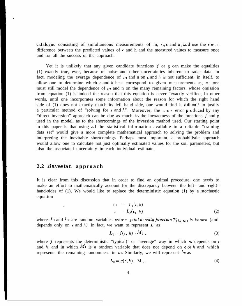
catalogue consisting of simultaneous measurements of m, n, c and h, and use the r,rn. s.difference between the predicted values of c and h and the measured values to measure onceand for all the success of the approach.

Yet it is unlikely that any given candidate functions j or g can make the equalities(1) exactly true, ever, because of noise and other uncertainties inherent to radar data. Infact, modeling the average dependence of m and n on E and h is not sufficient, in itself, toallow one to determine which c and h best correspond to given measurements m, n: onemust still model the dependence of m and n on the many remaining factors, whose omissionfrom equation (1) is indeed the reason that this equation is never “exactly verified, In other

words, until one incorporates some information about the reason for which the right handside of (1) does not exactly match its left hand side, one would find it dif%cult to justifya particular method of “solving for c and h“. Moreover, the r.m,s. error produc,ed by any“direct inversion” approach can be due as much t~ the inexactness of the functions ~ and gused in the model, as to the shortcomings of the inversion method used. Our starting pointin this paper is that using all the statistical information available in a reliable “trainingdata set” would give a more complete mathematical approach to solving the problem andinterpreting the inevitable shortcomings. Perhaps most important, a probabilistic approachwould allow one to calculate not just optimally estimated values for the soil parameters, butalso the associated uncertainty in each individual estimate.

2.2 Bayesian approach

It is clear from this discussion that in order to find an optimal procedure, one needs tomake an effort to mathematically account for the discrepancy between the left– and right–hand-sides of (1), We would like to replace the deterministic equation (1) by a stochasticequation

m = I.l(c, h).n = L~(c, h) (2)

where L1 and L2 are random variables whose joint density functio7t P(L1 ,L2) is known (anddepends only on c and h). In fact, we want to represent LI as

1.1 == f(c, h) o Ml , (3)

where ~ represents the deterministic “typical)’ or “average” way in which m depends on cand h, and in which All is a random variable that does not depend on c or h and whichrepresents the remaining randomness in m. Similarly, we will represent L2 as

Lz =: g(c,h) . M 2 . (4)

4

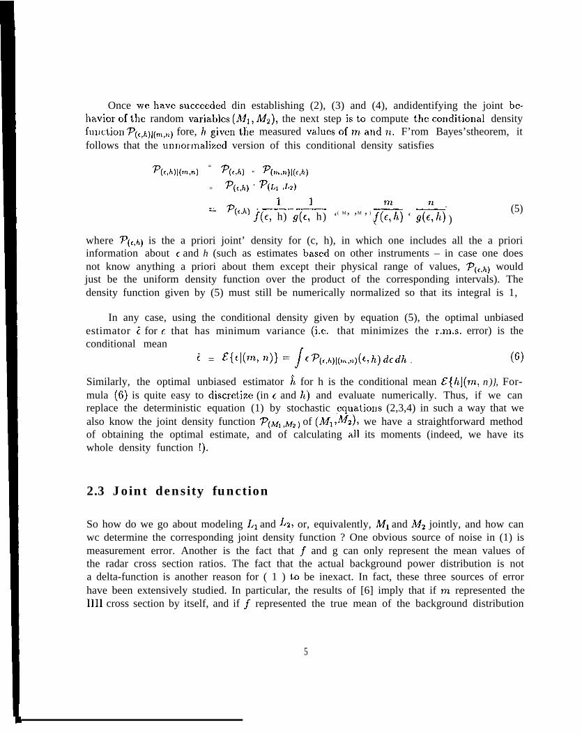
Once wehavesucceecle din establishing (2), (3) and (4), andidentifying the joint be-haviorofthe random variables (~l,lkl~), the next step isto compute thcconditional densityf’unction ~(,,~)l(n,,n) fore, hgiventhe measured valuesofrnandn. F’rom Bayes’stheorem, itfollows that the unnorrnalized version of this conditional density satisfies

qc,h)l(m,n) = qc,h) “ qm,n)l(c,h)= P(+) ‘ qL, J,,)

11. ——— —.-=(

— —‘(”h) f(e, h) g(t, h) ‘( M’ ’M ’ ) f(;h) ‘ g(;h) )

(5)

where ~(t,~) is the a priori joint’ density for (c, h), in which one includes all the a prioriinformation about c and h (such as estimates based on other instruments – in case one doesnot know anything a priori about them except their physical range of values, ~(,,~) wouldjust be the uniform density function over the product of the corresponding intervals). Thedensity function given by (5) must still be numerically normalized so that its integral is 1,

In any case, using the conditional density given by equation (5), the optimal unbiasedestimator ; for c that has minimum variance (i.e. that minimizes the r.m.s. error) is theconditional mean

~ = ~{~l(m, n)} == / c~(c,MI(m,n)(c) h)~~~~ . (6)

Similarly, the optimal unbiased estimator jt for h is the conditional mean Z{hl(m, n)}, For-mula (6) is quite easy to discretize (in c and h) and evaluate numerically. Thus, if we canreplace the deterministic equation (1) by stochastic ,cquations (2,3,4) in such a way that wealso know the joint density function ‘P(M1 ,M, ) of (ill] ,iM2)1 we have a straightforward methodof obtaining the optimal estimate, and of calculating all its moments (indeed, we have itswhole density function !).

2.3 Joint density function

So how do we go about modeling 1.1 and L2, or, equivalently, All and MZ jointly, and how canwc determine the corresponding joint density function ? One obvious source of noise in (1) ismeasurement error. Another is the fact that j and g can only represent the mean values ofthe radar cross section ratios. The fact that the actual background power distribution is nota delta-function is another reason for ( 1 ) to be inexact. In fact, these three sources of errorhave been extensively studied. In particular, the results of [6] imply that if m represented the1111 cross section by itself, and if ~ represented the true mean of the background distribution

5

of nt, then the density function PM of the random variable M = rn/j(c, h) is

q~/4)(~+P)/2

PM(Z) = —r@qr(~l)

,#+iI-1)/2 ]{.-h?(2&) (7)

where K denotes the modified Bessel function of the second kind. In (7), we have alsoassumed that N radar looks were used to produce m, that the fading has Rayleigh charac-teristics, and that the background power level is I’-distributed with relative variance 1 /jL,

If we were to use this result in our case, where m and n are ratios of backscattering cross-sections, we would need to assume that each of &ll and M2 in equations (3,4) is the ratioof two random variables distributed according to (7). There are several reasons not to dothis directly. First, the assumption that the background power level is I’-distributed is notalways necessarily valid ([1 3]). Other distributions would produce different expressions for

PM. Second, the presence of a Bessel function in expression (7) makes it unnecessarily dif%-cult to use in practice. In fact, in the two extremes where p is very large (corresponding tothe case where the variance of the background level is very small) or N is very large (corre-sponding to the case where a large number of looks are used to average out uncertainties inthe backscattered power), (7) reduces to a l’-distribution. Finally, the candidate functions

j and g may well turn out to be poor approximations of the true means. Indeed, even ifone used a very accurate method to estimate the sample mean, one remains vulnerable tomeasurement error, and to contamination of the measurements by unknown scatterers onthe surface (‘(debris”, etc).

Taking all these considerations into account, it is neither unreasonable nor arbitrarilyrestrictive to assume that the measurements nl and n are related to c and h by equations(2,3,4), in which

● in the case where the measured variable is the received power (at the HH–, HV– orVV-polarization), each M~ is itself I’-distributed, these distributions being mutuallyindependent.

● in our case, where the measured variables are ratios of received powers, each Mi isdistributed like the ratio of the two corresponding (independent) I_’ distributions.

To determine the joint density function ‘P(~, ,~,, for (Ml ,M2), we will use a reliable set ofsimultaneous measurements of m, n, c and h, and test if this data is consistent with ourassumptions about M, The model for the M i’s is still not completely specified: indeed, theparameters of the I’-distributions involved must still be chosen. As we shall see in the nextsection, there is an optimal way to determine these parameters from the data catalogue.Moreover, it will turn out that the a priori assumptions that we make about theexact form of the distribution of the Mi’s are ultimately not crucial: any finalexpression that we settle on for the density function of the M i’s can and will be tested for

6

goodness-of-fit with the measurements ([2]). The problem of determining the parametersin the I’-distributions and testing the consistency of the resulting density function ?(~l ,~z)with the data is addressed in detail in the next section,

3 Joint density for the Michigan model

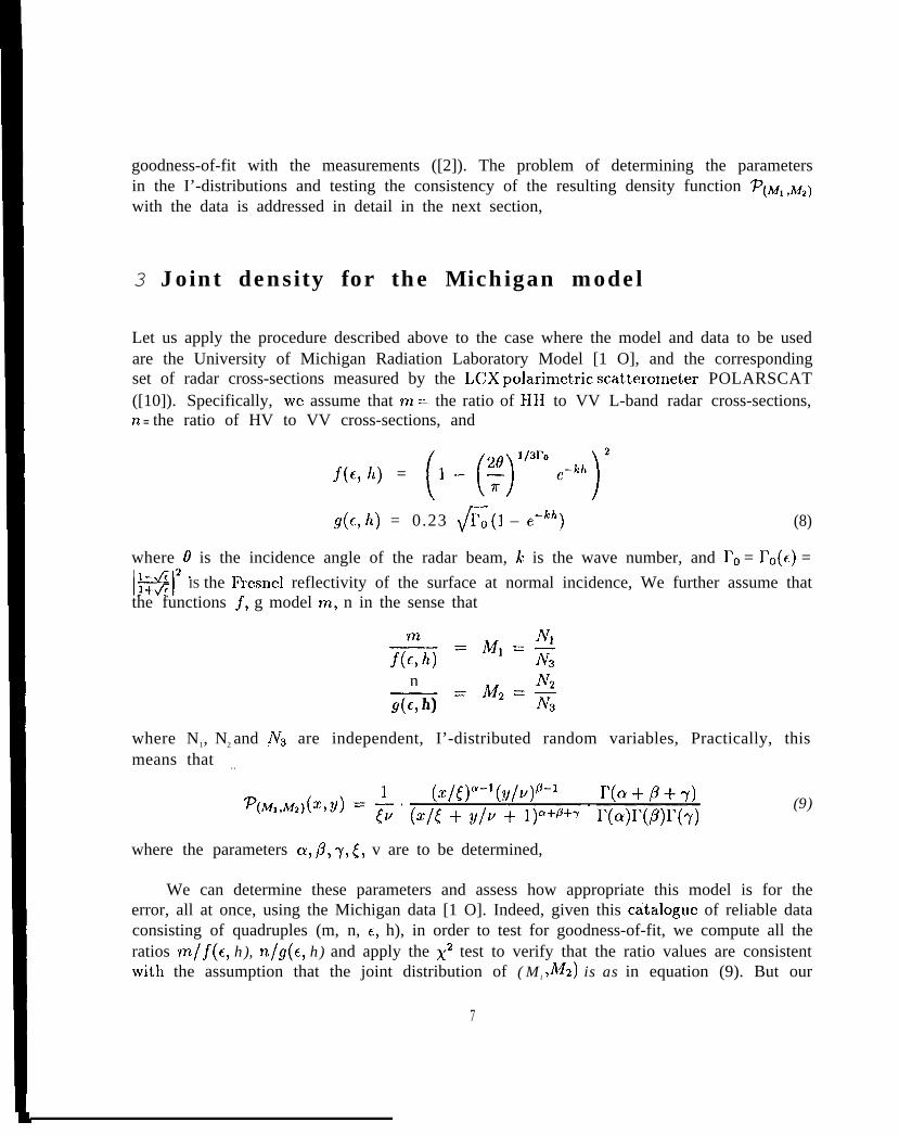
Let us apply the procedure described above to the case where the model and data to be usedare the University of Michigan Radiation Laboratory Model [1 O], and the correspondingset of radar cross-sections measured by the I,CX polarimetric scatterometer POLARSCAT([10]). Specifically, we assume that rn = the ratio of HII to VV L-band radar cross-sections,n = the ratio of HV to VV cross-sections, and

f(c, h) = (,_ y’)l,,r’’e-kh)’g(c, h) = 0.23 fi(l – e-~~) (8)

where O is the incidence angle of the radar beam, k is the wave number, and 1’0 = I’O(c) =

1+11-(’.1+ c IS the Fresnel reflectivity of the surface at normal incidence, We further assume that

the functions j, g model m, n in the sense that

N1—= Ml=Ef(;h)

n Nz—= M2=Xg(c, h)

where N1, N2 and N, are independent, I’-distributed random variables, Practically, thismeans that . .

where the parameters a, ~, ~, ~, v are to be determined,

(9)

We can determine these parameters and assess how appropriate this model is for theerror, all at once, using the Michigan data [1 O]. Indeed, given this catalogue of reliable dataconsisting of quadruples (m, n, t, h), in order to test for goodness-of-fit, we compute all theratios m/~(c, h), n/g(c, h) and apply the X2 test to verify that the ratio values are consistentwith the assumption that the joint distribution of ( Ml ,M2) is as in equation (9). But our

7

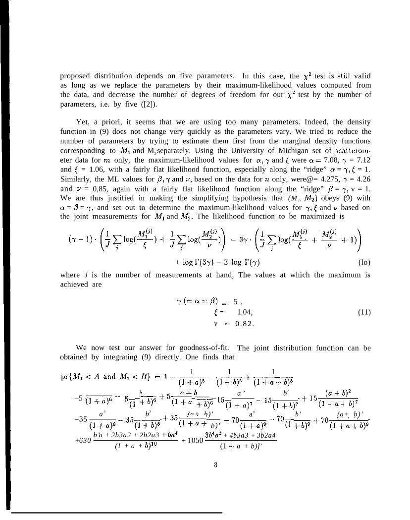
proposed distribution depends on five parameters. In this case, the Xz test is still validas long as we replace the parameters by their maximum-likelihood values computed fromthe data, and decrease the number of degrees of freedom for our Xz test by the number ofparameters, i.e. by five ([2]).

Yet, a priori, it seems that we are using too many parameters. Indeed, the densityfunction in (9) does not change very quickly as the parameters vary. We tried to reduce thenumber of parameters by trying to estimate them first from the marginal density functionscorresponding to &fl and M2 separately. Using the University of Michigan set of scatterom-eter data for m only, the maximum-likelihood values for a, ~ and ~ were a = 7.08, ~ = 7.12and ~ = 1.06, with a fairly flat likelihood function, especially along the “ridge” a = ~, ( = 1.Similarly, the ML values for /?, -y and v, based on the data for n only, were@= 4.275, ~ = 4.26and v = 0,85, again with a fairly flat likelihood function along the “ridge” /? = ~, v = 1.We are thus justified in making the simplifying hypothesis that (M l, MQ) obeys (9) witha = /? = 7, and set out to determine the maximum-likelihood values for ~, ~ and v based onthe joint measurements for A41 and &fz. The likelihood function to be maximized is

+ log I’(3~) – 3 log ~(~) (lo)

where J is the number of measurements at hand, The values at which the maximum isachieved are

7(=a=p) ~ 5 ,( == 1.04, (11)

v = 0 .82 .

We now test our answer for goodness-of-fit. The joint distribution function can beobtained by integrating (9) directly. One finds that

1pr{Ml<A and Alz<B}=l– — ——

(l+a)’ (l~b)’+(l+~+b)’

–5 a b a+b a ’ b2

+15 (a+b)2(l+a)’– 5(] +b)’+5(l+a+ b)’ 15~] +a)7 ‘15(l+b)7

—— _(l+u+b)’

–35a3 b3 (a+ b)’ a’ b’ (a+ b)’

(l+a)’ ‘35(l+b)8 ‘35(l+a+ b)’ ‘70(l+a)9 ‘70(] +b)g+70(]+a+b)gb’a + 2b3a2 + 2b2a3 + ba’ 3b4a2 + 4b3a3 + 3b2a4

+630(1 + a + b)’”

+ 1050(1 i- a + b)]’

8

b4a3 + b3a4 b4a4

‘11550(1 +a+ b)]’ + 34650(1+ a + b)’s(12)

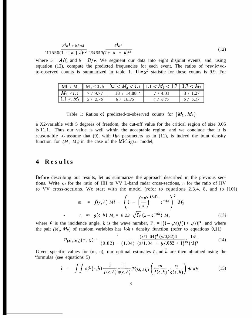
where a = A/~, and b = 13/v, We segment our data into eight disjoint events, and, usingequation (12), compute the predicted frequencies for each event. The ratios of predicted-to-observed counts is summarized in table 1. ‘1’hc X2 statistic for these counts is 9.9. For

Ml \ M2 M 2 < 0 . 5 o.5<M2<l. i 1.1< MZ<I.7 1.7<M2

Ml <1.1 7 / 9.77 18 / 14,88 ‘ 7 / 4.03 3 / 1,271.1 <Ml 5 / 2.76 6 / 10.35 4 / 6.77 6 / 6,17

Table 1: Ratios of predicted-to-observed counts for (Ml , Mz)

a X2-variable with 5 degrees of freedom, the cut-off value for the critical region of size 0.05is 11.1. Thus our value is well within the acceptable region, and we conclude that it isreasonable to assume that (9), with the parameters as in (11), is indeed the joint densityfunction for (M l, M2) in the case of the h4ichigan model,

4 Results

13efore describing our results, let us summarize the approach described in the previous sec-tions. Write m for the ratio of HH to VV L-band radar cross-sections, n for the ratio of HVto VV cross-sections. We start with the model (refer to equations 2,3,4, 8, and to [10])

m = f(c, h) Ml =: []_ [$13r0e-j2M1

. . n = g(c, h) M2 = 0.23 fi(l – e-~~) M2 (13)

where O is the incidence angle, k is the wave number, I’. = 1(1 – ~)/(1 + @)12, and wherethe pair (M l, Mz) of random variables has joint density function (refer to equations 9,11)

~(M,,M2)(~) v) =(x/1 .04)4 (y/0,82)4.—

(0.82) ~ (1.04) (z/1.04 + y/.O82 + 1)15 (;;;3,— (14)

Given specific values for (m, n), our optimal estimates t and ~ are then obtained using the‘formulas (see equations 5)

9

(15)

A=/1

1 1h7qE, /2) —-— (——)f(t, h) g(c, h) ‘(M]’M’) f(;h) ‘ g(;h) ‘Calf’ ‘ (16)

and t hc corresponding error bars are given by

The a priori density function T(c, h) will typically be assumed uniform over a rectangle in the(c, h)-plane. The integrals can be computed numerically. We are finally ready ‘to describethe results of this approach.

4.1 Optimal estimates:

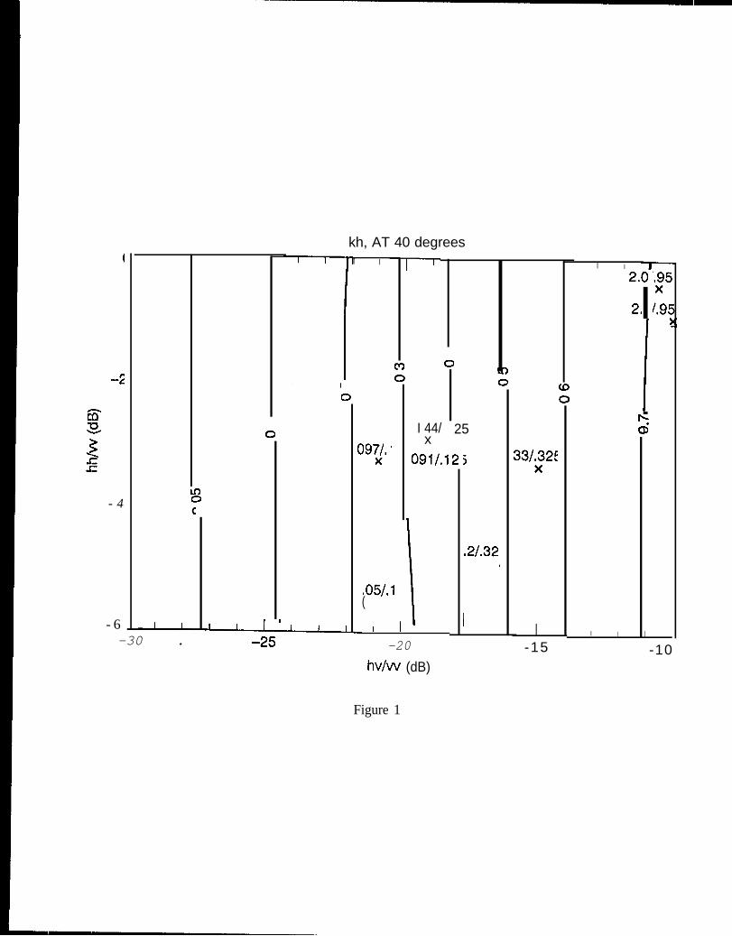
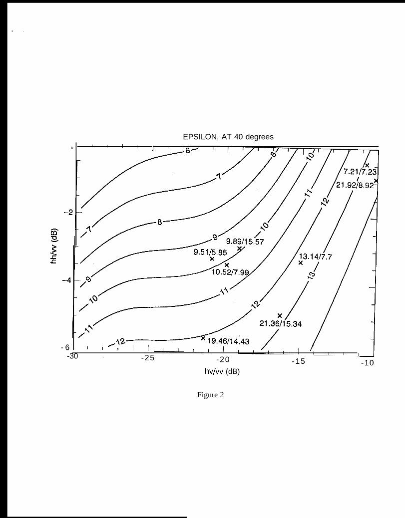
Figure 1 (resp, 2) is a contour plot of the optima.] estimate (h (resp. f) of kh (resp. c), as afunction of the cross section ratios m and n at O = 40°. The values of kh and t were obtainedusing our Bayesian approach, and starting with an a priori density function ~(c, h) that isuniform over the rectangle 2 < c < 20, 0 ~ kh < 1. Overlaid on the contour plot of figure1 (resp. 2) are those samples of the Michigan data that were collected at 40° incidence, eachaccompanied by the value of kh (resp. E) computed according to the inversion algorithmproposed in [1 O], as well as the measured values, At 40°, the value of kh calculated by thedirect inversion algorithm falls within 25% of the measured value in four out of the eightsamples, but it misses by 1007o in three cases. Our approach is not visibly more accurate.Similarly, the estimates of e do not appear to be very accurate,

4.2 Error bars:

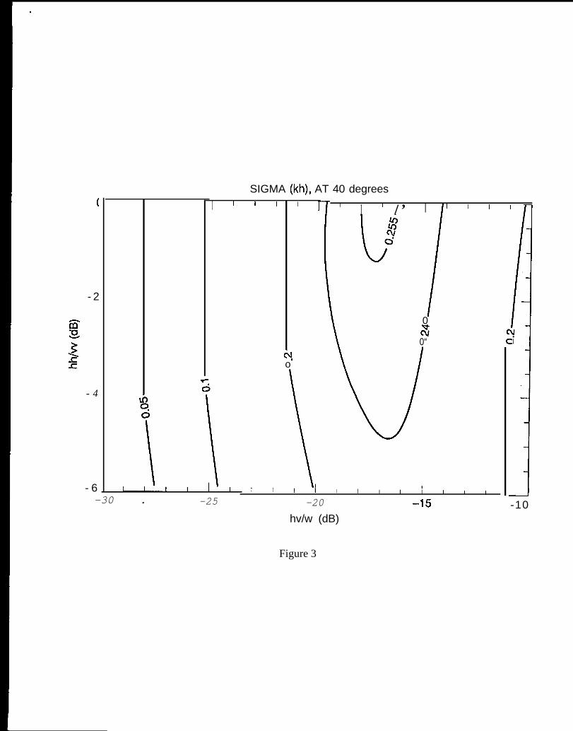
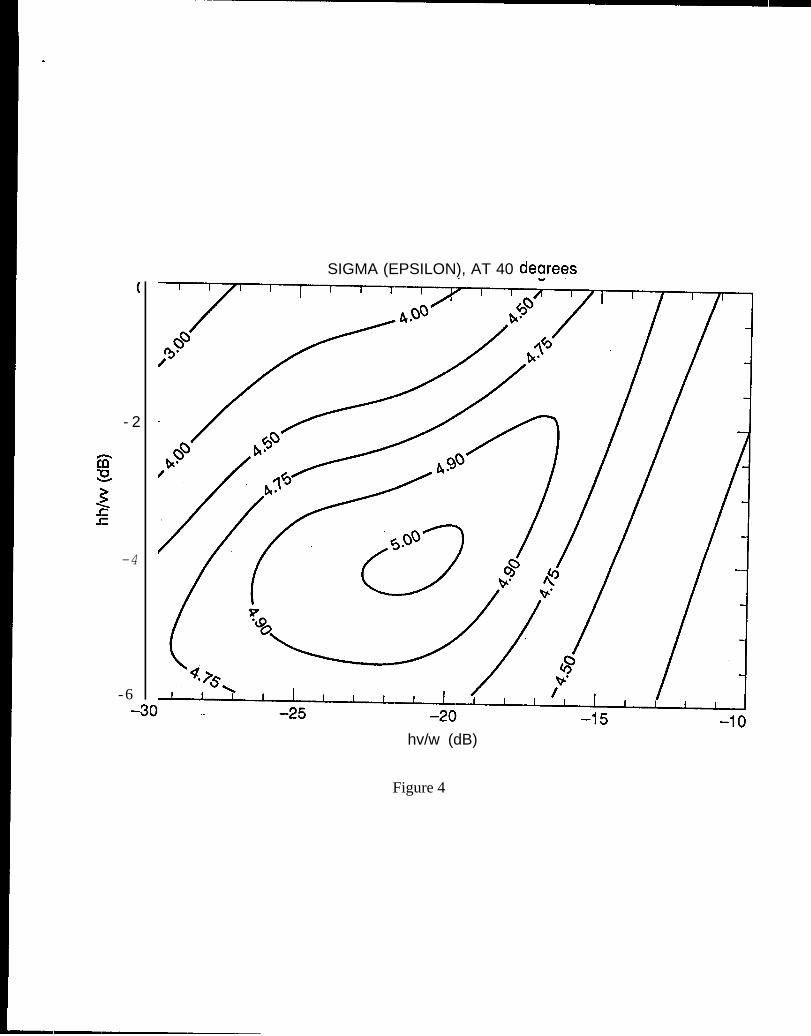
One way to measure the accuracy of the model functions f and g quantitatively is to lookat the variance of the conditional density function, Indeed, these variances quantify theuncertainties in the estimates obtained by using the optimal approach. Figures 3 and 4 showthe r.m.s. uncertainty in the estimates of kh and c respectively. In this case, the modelconsisting of the function ~ and g of equation (8) can be considered “useful” if the r.m,s.uncertainty of the estimates that we obtain with it is smaller than the a priori uncertaintymade by assuming that c and kh are uniformly distributed, i.e. if the r,m.s, uncertainty in.? is smaller than (2o — 2)/@ ~ 5,2, and if the r.m, s. uncertainty in kh is smaller than

10

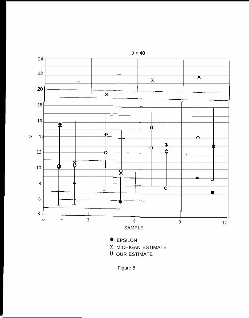
(1 – 0)/fi N 0,29, Figures 3 and 4 show that this is indeed achieved everywhere. Whileit is encouraging to verify that using the model is an improvement over chosing values for Eand kh at random, it should be noted that the relative uncertainty in the estimates is quitelarge, Indeed, figure 3 shows that if the absolute value of the HH-to-VV ratio n is less than21 d13, the 1. a uncertainty in the estimate of kh exceeds 0.2, But according to figure 1,when 72 is around -20 dB, the optimal estimate of kh is itself around 0.3. Its 1. a uncertaintyis therefore close to 100VO ! Overall, one can see from figures 1 and 3 that the smallest thatthe relative uncertainty in the estimate of kh gets is about 30%, when In! is less than 13 dB.On the other hand, figures 2 and 4 imply that the. r.m.s. relative uncertainty in the case of cis never worse than 50Y0, Although still somewhat high, this value seems encouraging. Yet,in the case of c, one is typically interested in differentiating between ‘iwet” and Cfdry” soil.Figure 5 colnpares the estimates for c based on the actual measurements in the Michigandata, showing side-by-side four pairs of samples. Each pair represents two measurements atthe same site, one when the soil was “wet” , followed by another when it was “dry”. Notethat the estimates for the first pair would erroneously indicate drier conditions on the firstday. The “spread” for the remaining cases between the optimal estimates on the dry andwet cases is not very significant in comparison with the size of the r.m.s. uncertainty. In fact,the wet–dry difference is typically less than 1/4 of the r,m,s. uncertainty in the estimate ofc, ‘l’his implies that the model will typically allow little discrimination between “wet” and“dry” soil.

4,3 Fine-tuning the initial model:

The results above illustrate the direct application of our estimation approach, and its abilityto quantify the uncertainty in the estimates one obtains using a particular model. In thiscase, it turned out that this uncertainty is rather large. Let us now try to use our method tohelp improve the estimates. So far, we have been using the model expressed in equation (8).One way to improve our estimates is to tune the parameters in t,hat model to the situationat hand. Specifically, one can postulate a n~odel of the form

f (c, h) = (,_ (Xy’’.-kh)’

g(t, h) = bI’oc (1 – c#) (19)

together with a probability density function ~(~1 ,~,) for the observed ratios (m/~, n/g) ofthe form

(20)

11

as before, then go on to determine a, b, c and N in order to maximize the likelihood ofobserving the radar cross sections reported in the Michigan data. In section 2, we derivedthe equation relating the density function ~(~1 ,I,,)(nz, n) for the observed HH-to-VV andII V-to-VV cross section ratios (m, n) to the density function ~(~1 ,~,). In fact, equation (5)states that

(21 )

~’he Michigan data include 32 observations at L-band with incidence angles between 30 and60 degrees. Calling these observed ratios { (mj, nj ) , ~ = 1, . . . ,32}, we arethe values of a, h, c, N which maximize

thus lead to find

(B ‘P(I.l,L,)(~nj,nj) = ii f(,~,~j)~~jJ ‘(M’M’) f(c~jllj)’ !7(~~Vhj)j=l j=l ‘ )

32(n2j/.f(6j, ‘j)) ‘-1 (~j/g(~jj hj))N-’ I’(3N)

= j!! .f(’t~ ‘j)d~ F/f(’j, ‘j) + nj/9(~j, ‘j) + 1)3N r(N)3

1 r(3N)

(

(mj/.f(cj, ‘j)) “ (T1j/9(6j, ~j)) N

= i i — — —

)(22)

j=l ‘j ‘j ‘(N)3 (mj/f(cjt ‘j) + ‘j/9(6j> ‘j) + 1)3

= (54 “m” (E(~j/f(~jj~j)+,j/g(j~j)+-l)’)’v

(mj/.f(Ej, ‘i)) “ (nj/9(’j, ‘j))

It is apparent from this last equation that the probIem of finding the optimal values of a, b, cdecouples from the problem of finding the most suitable N. Indeed, to maximize (22), wemust find the values of a, b, c which maximize

(mj/f(ej, ‘j)) “ (nj/9(ej, ‘j))B ((mj/.f(6j,hj) + nj/9(~j,~~j) + 1)3j=l )and that value of N which then maximizes

()1’(3N) 3 2 ~fNl’(N)’ “

(23)

(24)

where K is the value of expression (23) when a, b, c take on their optimal values. Thisdecoupling is in fact expected: the problem of finding the “right” values of the parametersa, b, c should consist in matching the postulated form for ~ and g to the sample mean of thedata at hand, while the problem of finding the “right” value of N involves quantifying howclosely the “best” model then fits the data,

12

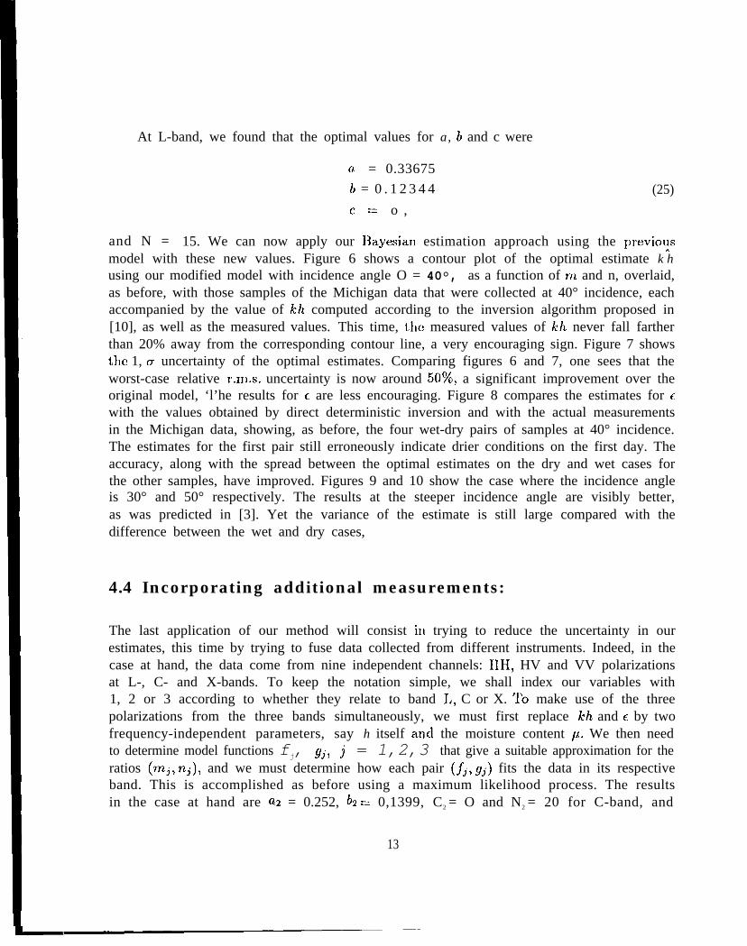
At L-band, we found that the optimal values for a, b and c were

a = 0.33675

b = 0 . 1 2 3 4 4 (25)

c= o ,

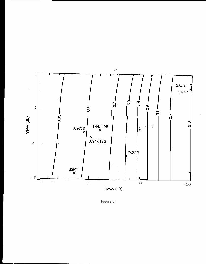
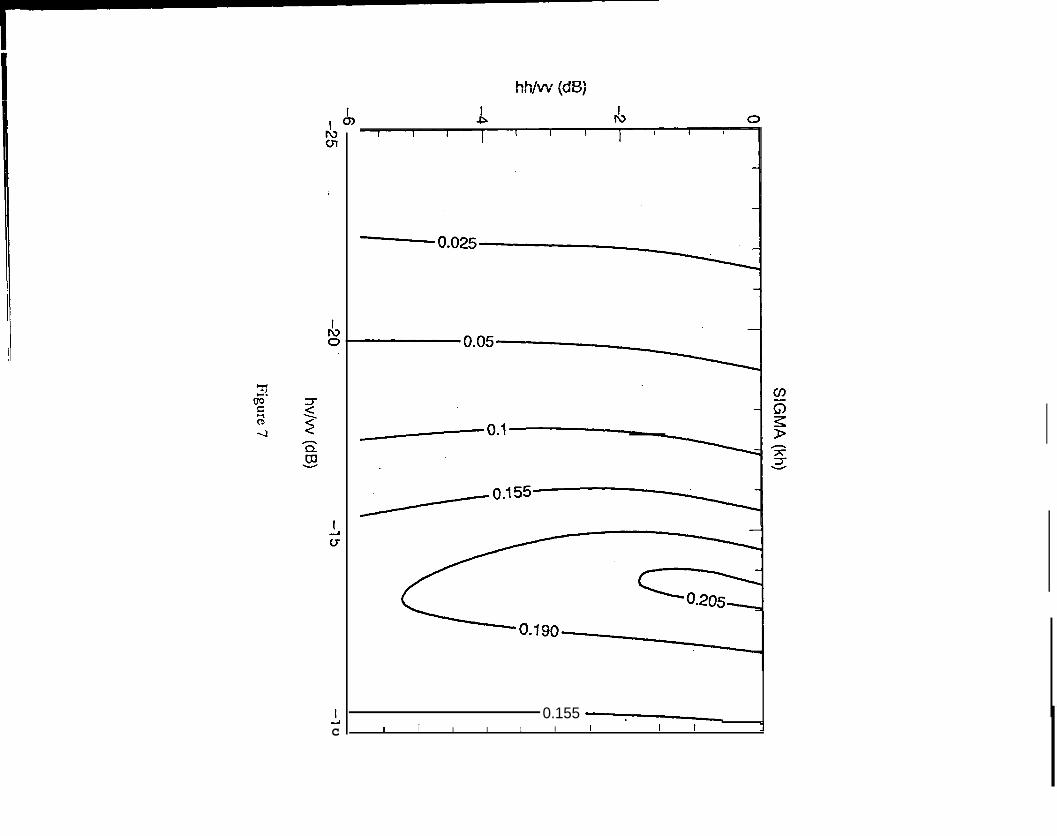
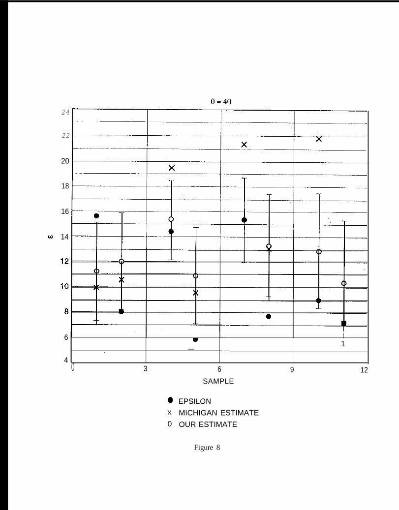
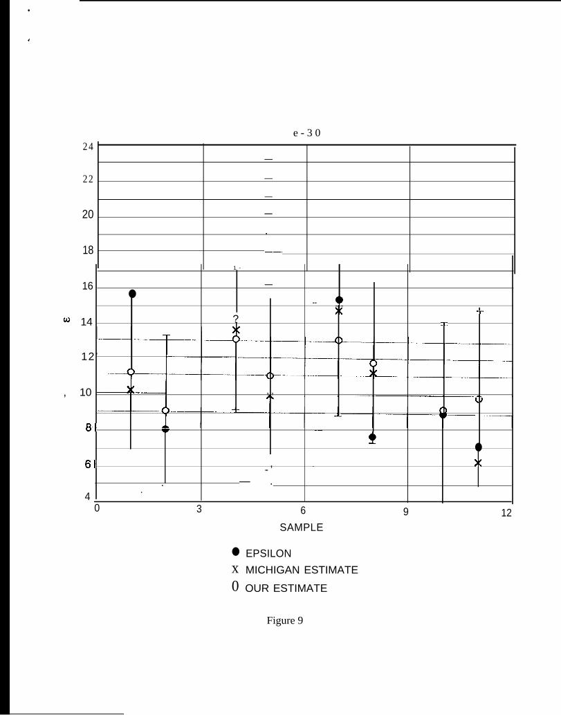
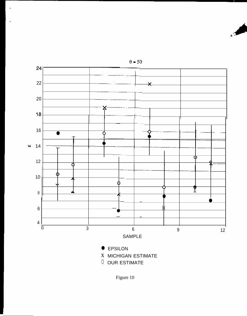
and N = 15. We can now apply our Bayesian estimation approach using the previo~smodel with these new values. Figure 6 shows a contour plot of the optimal estimate k husing our modified model with incidence angle O = 40°, as a function of m and n, overlaid,as before, with those samples of the Michigan data that were collected at 40° incidence, eachaccompanied by the value of kh computed according to the inversion algorithm proposed in[10], as well as the measured values. This time, tile measured values of kh never fall fartherthan 20% away from the corresponding contour line, a very encouraging sign. Figure 7 showsthe 1, a uncertainty of the optimal estimates. Comparing figures 6 and 7, one sees that theworst-case relative r,m.s. uncertainty is now around 50Y0, a significant improvement over theoriginal model, ‘l’he results for ~ are less encouraging. Figure 8 compares the estimates for cwith the values obtained by direct deterministic inversion and with the actual measurementsin the Michigan data, showing, as before, the four wet-dry pairs of samples at 40° incidence.The estimates for the first pair still erroneously indicate drier conditions on the first day. Theaccuracy, along with the spread between the optimal estimates on the dry and wet cases forthe other samples, have improved. Figures 9 and 10 show the case where the incidence angleis 30° and 50° respectively. The results at the steeper incidence angle are visibly better,as was predicted in [3]. Yet the variance of the estimate is still large compared with thedifference between the wet and dry cases,

4.4 Incorporating additional measurements:

The last application of our method will consist ill trying to reduce the uncertainty in ourestimates, this time by trying to fuse data collected from different instruments. Indeed, in thecase at hand, the data come from nine independent channels: HH, HV and VV polarizationsat L-, C- and X-bands. To keep the notation simple, we shall index our variables with1, 2 or 3 according to whether they relate to band 1., C or X. To make use of the threepolarizations from the three bands simultaneously, we must first replace kh and c by twofrequency-independent parameters, say h itself ancl the moisture content p. We then needto determine model functions fj, gj, j = 1,2,3 that give a suitable approximation for theratios (mj, nj), and we must determine how each pair (jj, gj) fits the data in its respectiveband. This is accomplished as before using a maximum likelihood process. The resultsin the case at hand are a2 = 0.252, b2 = 0,1399, C2 = O and N2 = 20 for C-band, and

13

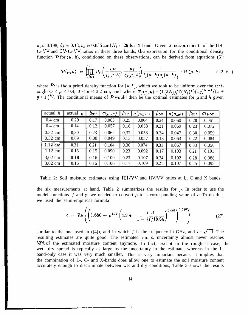
a3 = 0.198, h3 =0.13, c3=0.035and lV3=29for X-band. Given 6measurements of the HH-to-VV and HV-to-VV ratios in these three bands, the expression for the conditional densityfunction 7 for (p, h), conditioned on these observations, can be derived from equations (5):

((P(/!i,h) == fi 7’j — - ) 1

&Z~)’ 9A: }’J ~j(l’, h)9j(P) h’) )‘ P&L, h) ( 2 6 )

j=l

where 70 is the a priori density function for (p, h), which we took to be uniform over the rect-angle O < p < 0.4, 0 < h < 3.2 Cm, and where Tj(z, y) = (r(3Nj)/1’(Nj)3 )(xy)~~-l/(~ +y + 1 )~~. The conditional means of ~ WOUIC1 then be the optimal estimates for ~~ and h given

actual h actual p fi300 CT(~L300) j j1400 I 0(~L400 ) j’1500 CT(}1500 ) j&oO @600 )

0,4 cm 0.29 0.17 0.063 0.25 0,064 0.24 0.060 0.28 0.0610.4 cm 0.14 0.12 0.057 0.18 0.058 0.21 0.069 0.23 0.072

1 ,

0.32 cm 0,30 0.23 0.062 0,32 0.053 0.34 0.047 0.30 0.0590.32 cm 0.09 0.08 0.049 0.13 0.057 0.13 0.063 0.22 0,084

Imrn 0.31 0.21 0.104 0.30 0.074 0.31 0.067 0.33 0.0561 1

1,12 cm 0.15 0.15 0.090 0.23 0.092 0.17 0.103 0.21 0,1013,02 cm 0!19 0.16 0,109 0.23 0.107 0.24 0.102 0.28 0.0883.02 cm 0.16 0.16 0.106 0,17 0.109 0.21 0.107 0.25 0.095

Table 2: Soil moisture estimates using HH/VV and HV/VV ratios at L, C and X bands

the six measurements at hand, Table 2 summarizes the results for p. In order to use themodel functions f and g, we needed to convert p to a corresponding value of c. To do this,we used the semi-empirical formula

~ t= Re((l,686+/116~.9+i+ ~~}1864)00’5)153’) (27)

similar to the one used in ([4]), and in which ~ is the frequency in GHz, and i = fi. Theresulting estimates are quite good. The estimated r.m, s. uncertainty almost never reaches5070 of the estimated moisture content anymore. In fact, except in the roughest case, thewet—dry spread is typically as large as the uncertainty in the estimate, whereas in the L-band-only case it was very much smaller. This is very important because it implies thatthe combination of L-, C- and X-bands does allow one to estimate the soil moisture contentaccurately enough to discriminate between wet and dry conditions, Table 3 shows the results

14

actual h h~o. a(h300) halo. -j h~o. a(h~o. ) h~o. u(h~o. )

0.40 0.29 0.065 0.36 0.081 0.36 0.079 0.38 0.0760.40 0,29 0.063 0.38 0.091 0.60 0.160 0.66 0.165

0.32 0.22 0.044 0,3F 0.077 0.35 0.069 0,43 0,0890.32 0.29 0.061 0,47 0.121 0.73 0.226 1.21 0.408

1.12 1.39 0.494 1.09 0,365 1.17 0,354 1.02 0.2461.12 0.79 0.261 1.13 0.434 2,26 0,582 2.33 0.557

3.02 2.59 0.467 2.68 0.416 2.70 0.407 2.70 0.3913.02 1,97 0.615 2.38 0.550 2,44 0.526 2.55 0.466—

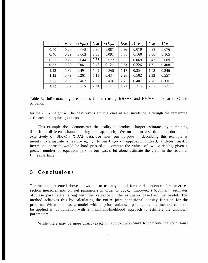
Table 3: Soil r.m.s. height estimates (in cm) using lIH/VV and HV/VV ratios at I,, C andX bands

for the r.m.s. height h. The best results arc the ones at 40° incidence, although the remainingestimates are quite good too.

This example does demonstrate the ability to produce sharper estimates by combiningdata from different channels using our approach, We intend to test this procedure moreextensively on SIR-C / X-SAR data. For now, our purpose in describing this example ismerely to illustrate a feature unique to our 13ayesian approach: indeed, a deterministicinversion approach would be hard pressed to compute the values of two variables, given agreater number of equations (six in our case), let alone estimate the error in the result atthe same time.

5 Conclusions. .

The method presented above allows one to use any model for the dependence of radar cross-section measurements on soil parameters in order to obtain improved (‘(optimal”) estimatesof these parameters, along with the variance in the estimates based on the model. Themethod achieves this by calculating the entire joint conditional density function for theproblem. When one has a model with a priori unknown parameters, the method can stillbe applied in combination with a maximum-likelihood approach to estimate the unknownparameters.

While there may be more direct (exact or approximate)

15

ways to compute the conditional

mean, calculating the conditional density itself is quite interesting and useful; Indeed, aswas demonstrated in the case of the combination of L- C- and X- band measurements, thisapproach can be used to quantify the improvement afforded by incorporating a particularmeasurement, by comparing the conditional (minimal) variance of the density function thatis conditioned on this particular measurement with the unconditional one to get a first-ordermeasure of the utility of using the measuremelit in question. Perhaps equally important,the last application demonstrated how one can use the conditioned density as a new a prioridensity function and incorporate observations from additional instruments by applying thisalgorithm repeatedly, each time updating the density function from the previous step inthe data fusion. We intend to test this approach more extensively on the data that will begathered by the SIR-C / X-SAR Space Shuttle experiment.

We are currently evaluating different models for the dependence of active radar measure-ments (at various frequencies and polarizations) on the soil parameters. More specifically,

we use our method to compare the variance of the optimal estimates obtained using the var-ious models under consideration. In addition, the results in the bare-soil case presented thispaper encourage us to believe that the method can be extended to account for more complexsources of randomness in the measurements, such as the presence of vegetation. Finally, weintend to apply our approach to optimally fuse passive radiometric measurements togetherwith the active radar data to obtain estimates of the soil parameters that, it is hoped, willhave a correspondingly smaller variance.

6 Acknowledgements

We wish to thank Professors Fawwaz Ulaby and Kamal Sarabandi, and the Radiation I,abo-ratory of the Department of Electrical Engineering and Computer Science at the Universityof Michigan for graciously sharing their data with us. ‘1’his work was performed at the JetPropulsion Laboratory, California Institute of Technology, under contract with the NationalAeronautics and Space Administration.

References

[1] A.A. Chukhlantsev and S,1. Vinokur: Radar sensing of soil and vegetation cover,Soviet J. Rem. Sens. 9, 1991, pp. 570-579,

.

[2]

[3]

[4]

[5]

[6]

[7]

[8]

[9]

[10]

[11]

[12]

[13]

[14]

R. D’Agostino and M.A. Stephens, Eds .: Goodness of fit techniques, M. I)ekker, NewYork, 1986.

M.C. Dobson and F.T. Ulaby: Active microwave soil rnoisttire research, I.E.E.E,Trans. Geossci. Rem. Sens. 24, 1986, pp. 23-28.

M,T. Hallikainen, F.T. Ulaby, M,C. Dobson, M.A, el-Rayes and L. Wu:’J4icrowavedielectric behuviorof wet soil-l, I. E.E,E. Trans. Geossci. Rem. Sens. 23, 1985, pp.25-34.

T.J. Jackson, K,G. Kostov and S.S. Saatchi: Rock fraction eflects on the interpretationof microwave emission jrcnn soils, I. E. E. F., Trans. Geosci. Rem. Sens. 30, 1992, pp.610-616.

D.J. Lewinski: Nonstationary probabilistic target and clutter scattering models,I. E.E.E. Trans. Ant. Prop. 31, 1983, pp. 490-498.

H.H, Lim, A,A. Swartz, H,A. Yueh, J,A. Kong, et al: Classification of earth terrainusing polarimetric synthetics apcrtum radar images, J. Geophys. Res. 94, 1989, pp.7049-7055.

M. Moghaddadm and S.S. Saatchi: An inversion algorithm applied to SAR data toretrieve surface parameters, Proc. IGARSS ’93, Tokyo, pp. 587-589.

E.G. Njoku and Y.H. Kerr: A semiempirical model for interpreting microwave emis-sion from semi-arid land surfcaces as seen from space, I. E.E. E. Trans. Geosci. Rem.Sens. 28, 1990, pp. 384-393.

Y, Oh, K. Sarabandi and F,T. Ulaby: An empirica~ m“odel and an inversion techniquefor radar sctittering from bare soil surfaces, I.E,E.E. Trans. Geosci. Rem. Sens. 30,1992, pp. 370-381.

C. Schmullius and R. Furrer: Some critical remarks on the use of C-band radar datajor soil moisture detection, Intl. J. Rem, Sens. 13, 1992, pp. 3387-3390.

L. Tsang, J.A. Kong, E.G. Njoku, D.H. Staelin and J.W. Waters: Theory for mi-crowave thermal emission from a layer of cloud or rain, I. E,E. E. Trans. Ant. Prop,25, 1977, pp. 650-657.

F.’l’. Ulaby and M.C. Dobson : Handbook of radar scattering statistics for terrain,Artech House, Norwood MA, 1989.

J.R, Wang and B.J. Choudhury : Remote sensing of soil moisture content over bamjicld at 1.4 GHz frequency, J. Geophys. Res, 86, 1981, pp. 5277-5282.

17

[15] J.J. van Zyl and C.F. Burnette : Baycsian classification oj polarimetric SAR imagesusing adaptive a-priori probabilities, Intl. J. Rem, Sens. 13, 1992, pp. 835-840.

18

kh, AT 40 degrees(

-2

- 4

-6

r I

)9~, ‘

.05/,1( I

I 44/x

191/.1

-L&_L- ,1I-30 . -20

25

j

,2/,32d

I

iI

33/;2:

-15

I I

2,(

2,

IIy

o

‘.:5

/,9

I I I

-10hvlvv (dB)

Figure 1

I1 .

EPSILON, AT 40 degreeso I I I 1

II

- 6 I I 1 I-30 ~ -25 -20 -15

hvlw (dB)-10

Figure 2

.

(

- 2

- 4

- 6

SIGMA (kh), AT 40 degrees

I I I I I r

d.o

)?

o,lll\, ,.-30 . -25

I I I / ’ 1’I I I II

\

/030“

1 I ! I I I I I I t I I-20 -15

Ii

i I

-10hv/w (dB)

Figure 3

.

SIGMA (EPSILON), AT 40 dearees(

- 2

-4

-6

hv/w (dB)

Figure 4

.

24

22

0=40

. .

—

x A— .—

18 —— .—

_— _____ —16

0.-

4 )— . — _ . .

Q) 14 4 1— _ _ ( )

)< ()12

()c)—.. — . . + .

—

10 A

a8 A h

A—

6.— . JR

6 —-. . _

—— ______

q~o - 3 6 9 12

●

x0

SAMPLE

EPSILON

MICHIGAN ESTIMATEOUR ESTIMATE

Figure 5

4

- 6

kh

C9

o“w-

0“

I

i

2/,3!

,33/x

-/,;,,,,,,

.097/,1 ,144~125x

,:91/,125

,06/,1x

–25 ~ –20 -15

52

2.0/,9!

2,1/,9

o

-10hv/w (dB)

Figure 6

c0.155 “~.

1 I I I 1 I t I I 1

0=4024

22

20

18

16

14

6 w . . I1

— ..—.40 3

●

x

0

6

SAMPLE

EPSILON

MICHIGAN ESTIMATE

OUR ESTIMATE

Figure 8

9 12

●

4

e - 3 024

—

22 —

—

20 —

.

18 ——1 -

16 —●

-- 9-r

w 14 ? -r

12’

, 10 , ,( )

8 w .—+

●

6 - ’ - > (

. — .4

.

0 3 6 9 12

●

x0

SAMPLE

EPSILON

MICHIGAN ESTIMATE

OUR ESTIMATE

Figure 9

24

22

20

18

16

QJ 14

12

10

8

0=50

-—,3----x.—

-——.——

.—— ——

●� ✎� �

1-

— .—— _

( )

()o

-——( )

7( .——

\# ( )n a

A ,A ●

— — ●

6 — )(

— —4

0 3 6 9 12

●

x0

SAMPLE

EPSILON

MICHIGAN ESTIMATEOUR ESTIMATE

Figure 10