Bayesian Estimation of Ordinary Differential Equation ...Some challenges exist in estimating ODE parameters. First of all, most ODEs are nonlinear and, with a few exceptions, have

Monte Carlo Methods Appl. ? (????), 1–17DOI 10.1515/mcma-????-??? © de Gruyter ????

Bayesian Estimation of Ordinary DifferentialEquation Models when the Likelihood has Multiple

Local Modes

Baisen Liu, Liangliang Wang and Jiguo Cao

Abstract. Ordinary differential equations (ODEs) are popularly used to model complexdynamic systems by scientists; however, the parameters in ODE models are often un-known and have to be inferred from noisy measurements of the dynamic system. Oneconventional method is to maximize the likelihood function, but the likelihood functionoften has many local modes due to the complexity of ODEs, which makes the optimizingalgorithm be vulnerable to trap in local modes. In this paper, we solve the global opti-mization issue of ODE parameters with the help of the Stochastic Approximation MonteCarlo (SAMC) algorithm which is shown to be self-adjusted and escape efficiently fromthe “local-trapping" problem. Our simulation studies indicate that the SAMC method is apowerful tool to estimate ODE parameters globally. The efficiency of SAMC method isdemonstrated by estimating a predator-prey ODEs model from real experimental data.

Keywords. Dynamical Model, Stochastic Approximation Monte Carlo, GlobalOptimization, System Identification..

2010 Mathematics Subject Classification. 62F15.

1 Introduction

Ordinary differential equations are often used to model the rate of change of a dy-namic process in time and/or space (expressed as derivatives). They are widely ap-plied to describe complex dynamic systems in many areas of science and technol-ogy such as engineering, physics, economics, pharmacokinetics, neurophysiology,and systems biology. The forms of ODEs are usually proposed based on the expertknowledge of the dynamic systems and scientific principles such as conservationof mass and energy, and the parameters in these ODEs generally have scientificinterpretations. On the other hand, the values of these parameters are typically un-known. One of the central problems in using ODEs is to estimate these parameters

This research was supported by the Liaoning Provincial Education Department (No.LN2017ZD001) to B. Liu and the discovery grants from the Natural Science and Engineering Re-search Council of Canada to J. Cao and L. Wang.

2 B. Liu, L. Wang and J. Cao

from the measurements of these dynamic systems in the presence of measurementerrors.

Some challenges exist in estimating ODE parameters. First of all, most ODEsare nonlinear and, with a few exceptions, have no analytic solutions. Many meth-ods have been developed to solve ODEs numerically, such as the Euler method andthe Runge-Kutta method [5]. In addition, the ODE solutions are often sensitive tothe values of ODE parameters. Consequently, the likelihood surface has manylocal modes, which will be illustrated in our application and simulation studies.The goal of this paper is to solve the global optimization issue with the help ofBayesian approaches.

A host of statistical approaches have been proposed to estimate ODE parametersfrom noisy data. [1] and [3] introduced a nonlinear least squares method, whichsearched for the optimal values of ODE parameters by optimizing the fitting ofthe numerical solutions of the ODEs to the data. Optimization is usually carriedout with gradient-based methods such as the Newton-Raphson method, but oftensuffers from convergence to local modes.

[29] suggested a two-step estimating procedure based on some classic nonpara-metric smoothing methods, which was later developed by [24], [21], [11], and[4]. This method avoids solving ODE numerically so that the burden of intensive-computations is reduced. However, the estimated ODE parameters often have alarge bias because the ODEs did not be involved in when estimating the deriva-tives. [23] developed a generalized profiling method, which used a nonparamet-ric function to represent the dynamic process. This method was shown to beable to obtain good estimates of the ODE parameters with the low computationalload. [22] proved that the generalized profiling estimates for ODE parametersare asymptotic efficient. [10] proposed a robust estimation method for estimat-ing ODE parameters. [9] extended the generalized profiling method to estimatethe time-varying parameters in ODEs. On the other hand, the generalized pro-filing method usually uses gradient-based methods and is hard to obtain globallyoptimized estimates for ODE parameters when the likelihood has multiple localmodes.

Recently, Bayesian methodology is quickly developed and has been appliedin numerous fields because it can answer complex questions cleanly and exactlyand provide more intuitive and meaningful inference [14]. The classic Markovchain Monte Carlo (MCMC) method in Bayesian statistics is then applied to in-fer the ODE parameters from noisy data [13, 17]. However, it is well known thatthe classical MCMC method is vulnerable to be trapped in local modes when thelikelihood surface is rugged, i.e., has a lot of local modes. Moreover, in high di-mensions of many parameters to sample, the random walk becomes inefficient dueto low rates of acceptance, poor mixing of the chain and highly correlated samples.

Estimating ODE Models 3

To overcome these obstacles, [6] proposed a population-based MCMC samplingprocedure called parallel tempering, which enabled the sampler to efficiently es-cape local posterior modes and hence worked well for sampling from multi-modaldistributions. However, as stated in Section 2.1 of [7], the posterior flatteningstrategies may lead to slower mixing and larger burn-in in the sampling process.Moreover, parallel tempering may fail if the prior information does not agree withthe features of the observed data. As a remedy, [7] proposed a smooth functionaltempering, which combines parallel tempering and model-based smoothing to de-fine a sequence of approximations to the posterior. These methods treat the tem-perature as an auxiliary variable. For high temperatures, the proposal distributionis broadened so that the problem of convergence to local modes is mitigated bysearching larger regions of the sampling space.

Different from the above approaches, in this article, we directly pursue the is-sue of maximizing the log-likelihood function of ODE parameters from the pointview of Monte Carlo optimization. The Monte Carlo optimization approach en-joys a long history and numerous Monte Carlo optimization approaches have beendeveloped, which include the gradient method, simulated annealing [15, 26], andthe stochastic approximation Monte Carlo (SAMC) method [19]. The gradientmethod requires a precise knowledge of the target function and easy to trap in thelocal modes, while the main difficulty of using simulated annealing lies in choos-ing the cooling temperature schedule.

In contrast, the SAMC method utilizes the past samples and, essentially, is adynamic importance sampling algorithm in which the trial distribution is learneddynamically from past samples. The SAMC method can self-adjust to escapefrom “trapping in" local multi-modes by partitioning sample space, setting desiredsampling distribution, and choosing appropriate gain factors. It has been shown tobe an extremely efficient tool to solve the “local-trap" optimization problem. Inthis paper, we develop the SAMC method to sample the posterior distribution ofODE parameters. In our simulation studies and real data analysis, we show that theSAMC method works very well for inference of complex nonlinear ODEs modelsand its implementation is very easy and convenient.

The remainder of this article is organized as follows. Section 2 introduces aBayesian model for statistical inference of ODE parameters, which is estimatedwith the SAMC method. The SAMC method is then demonstrated in Section 3by estimating a predator-prey dynamic model from real experimental data. Simu-lation studies are presented in Section 4 to illustrate the advantage of the SAMCmethod in comparison with the MCMC method. Conclusions are given in Section5.

4 B. Liu, L. Wang and J. Cao

2 Methodology

Consider the following dynamic ODEs model

dXi(t)

dt= gi(X(t)|β), t ∈ [Ts, Te], i = 1, . . . , I, (2.1)

where X(t) = (X1(t), . . . , XI(t))T denotes the vector of ODE variables, and β is

an unknown vector of parameters of the ODEs model. Let Xi(t|θ), i = 1, . . . , Idenote the solutions of the ODEs (2.1) where θ = (αT ,βT )T ∈ Θ with the ODEparameter values as β and the initial conditions as α. Let y = (y11, . . . , yInI

)T

be the vector of all observations and yij denote the observation for the i-th ODEvariable at tij , j = 1, · · · , ni, i = 1, . . . , I , which is assumed to follow someprobability distribution f(y|θ), for example, the normal distribution with the meanXi(tij |θ) and the variance σ2

i .

A popular approach to estimate θ based on y is to maximize the likelihoodfunction

L(θ|y) =I∏

i=1

ni∏j=1

f(yij |θ). (2.2)

Under the Gaussian assumption of yij ∼ N(Xi(tij |θ), σ2i ), i = 1, . . . , I, j =

1, . . . , ni, the likelihood function of θ based on y is given by

L(θ) =I∏

i=1

ni∏j=1

(σ2i )

−1/2 exp{− (yij −Xi(tij |θ))2

2σ2i

}. (2.3)

Define

U(θ) =

I∑i=1

ni∑j=1

{yij −Xi(tij |θ)}2

σ2i

, (2.4)

then finding the maximum likelihood estimate (MLE) of θ based on (2.3) is equiv-alent to minimizing the function U(θ).

Adopting the idea of Monte Carlo optimization, instead of minimizing (2.4)by classical approaches (e.g., gradient-based methods), in this article, we sug-gest to apply the SAMC method to simulate a trial distribution which is pro-portional to exp{−U(θ)}. Firstly, we partition the domain space Θ into somesubregions and seek to draw samples from each of the subregions with a pre-specified frequency. If this goal can be achieved, then the local-trap problem canbe avoided successfully. Assume that the parameter space, Θ, is partitioned intoM disjoint subregions, which are denoted by E1 = {θ : U(θ) ≤ u1}, E2 =

Estimating ODE Models 5

{θ : u1 < U(θ) ≤ u2}, . . . , EM−1 = {θ : uM−2 < U(θ) ≤ uM−1}, andEM = {θ : U(θ) > uM−1}, where u1, . . . , uM−1 are pre-specified real num-bers by users. In practice, the maximum difference in each subregion should bebounded by a reasonable number, say, 2, which ensures that the local MH moveswithin the same subregion have a reasonable acceptance rate.

Define g = (g1, . . . , gM )T , where gm =∫Em

exp{−U(θ)}dθ form = 1, . . . ,M .To present the idea clearly, we temporarily assume that gm > 0 for all m =1, . . . ,M , but, it is allowed for some subregions with gm = 0 in practice. De-fine a pre-specified frequency, say π = (π1, . . . , πM ) with 0 < πm < 1 and∑M

m=1 πm = 1. Generally, a uniform sequence of πm = 1/M,m = 1, . . . ,M ,is chosen, as in all examples of this article. If this goal can be achieved, then thelocal-trap problem is avoided essentially. To achieve this goal, we try to sample θfrom the following trial distribution

fg(θ) ∝M∑

m=1

πm exp{−U(θ)}gm

I(θ ∈ Em), (2.5)

where I(·) is an indicator function.

Obviously, the value of gm affects the probability of θ being sampled in thesubregion Em at each iteration. If a subregion is visited, say, Em, then g will beupdated according to some mechanism (see the details discussed later) such thatthe subregion Em has a smaller probability to be revisited and other subregionshave larger probabilities to be visited in the next iteration. This mechanism enablesthe algorithm to escape from local multi-mode very quickly.

In practice, gm is always unknown in sampling implementation, but it can beestimated together with sampling θ iteratively. Hence, the whole sampling pro-cedure consists of two steps: sampling in the Step 1 and updating weights in theStep 2. More detailed, let g(k)m denote the estimate of gm at the k-th iteration,g(k) = (g

(k)1 , . . . , g

(k)M )T , and θ(k) denote the sample of θ at the k-th iteration, then

we perform the following procedures in the (k + 1) -th iteration:(a) Sampling: sample θ(k+1) by a single Metropolis-Hastings update from the dis-tribution

fg(θ) ∝M∑

m=1

πm exp{−U(θ(k))}g(k)m

I(θ ∈ Em),

in the following three steps:(a.1) Generate θ ∗ in the sample space Θ according to a proposal distributionq(θ ∗;θ(k)).

6 B. Liu, L. Wang and J. Cao

(a.2) Calculate the ratio

r =fg(θ

∗)

fg(θ(k))

q(θ(k);θ ∗)

q(θ ∗;θ(k)).

(a.3) Set

θ(k+1) =

{θ ∗, with the probability min(1, r),θ(k), otherwise.

(b)Weight update: set

g(k+1) = g(k) exp{γ(k)(e(k) − π)},

where γ(k) is called the gain factor in the context of stochastic approximation [25].In practice, as in this article, we often choose

γ(k) =T0

max(T0, k), k = 1, 2, . . . , (2.6)

for some specified value of T0 > 1. The indicator vector e(k) = (e(k)1 , . . . , e

(k)M )T

with e(k)m = 1 if θ(k+1) ∈ Em and 0 otherwise.

A large value of T0 will force the sampler to reach all subregions quickly, evenin the presence of multiple local modes. Therefore, T0 should be set to a largevalue for a complex problem. For the nonempty subregion Ems, let fm be therealized sampling frequency, and f be the average sampling frequency. Define

εf = min{fm

f: m = 1, . . . ,M,Em 6= ∅

}.

An appropriate choice of T0 and the total iteration number N are chosen such thatthe sampling frequency of each nonempty subregion is not less than 80% of theaverage sampling frequency, that is, εf ≥ 80%. Once a run was checked not toconverge, we re-run the above iterations with a larger value of N and/or a largervalue of T0. In this article, the following scheme is adopted to update T0 andN : the number of total iteration N is increased to 2N , and T0 defined in (2.6) isincreased to 1.5T0.

Our method can give some estimation of the mean square error which cannotbe made smaller. Our method first partitions the parameter space according to therange of the mean square errors, U(θ), and then seeks to draw samples from each

Estimating ODE Models 7

of the subregions with a pre-specified frequency. At the same time, our methodallows for some subregions to be empty, i.e., some subregions are never visitedin a long sampling run. For example, if the subregions E1 = {θ : U(θ) ≤ u1},E2 = {θ : u1 < U(θ) ≤ u2},. . .,EK = {θ : uK−1 < U(θ) ≤ uK} are nevervisited in a long run, and EK+1 = {θ : uK < U(θ) ≤ uK+1} are visited withsome samples, then we can claim that the minimum mean square error is probablebetween uK and uK+1.

3 Application

It is of great interest in ecology to study the predator-prey interactions amongspecies [18,28]. Nonlinear ODE models display a similar set of dynamic behaviorsas ecological populations, such as coexistence at an equilibrium and a limit cycle[2], and hence are popularly used to model the predator-prey dynamic systems[20].

For example, an aquatic laboratory community containing two microbial specieshas studied by [12], [27], and [30]. This dynamic system is a nutrient-basedpredator-prey food chain, in which the growths of unicellular green algae, Chlorellavulgaris, are limited by the supply of nitrogen, and Chlorella are eaten by plank-tonic rotifers, Brachionus calyciflorus. The prey, Chlorella, and the predator, Bra-chionus, are growing together in replicated, experimental flow-through cultures,called chemostats. Nitrogen continuously flows into the system with the concen-tration, N∗, at the dilution rate, δ, and all components of the dynamic system areremoved from the chemostats at the same rate, δ.

[12] proposed a set of nonlinear ODEs to model consumer-resource interactionsbetween Chlorella, Brachionus, and the nitrogen resource. The nonlinear ODEsmodel can be expressed as follows

dN(t)dt = δ(N∗ −N(t))− FC(N(t))C(t),

dC(t)dt = FC(N(t))C(t)− FB(C(t))B(t)/ε− δC(t),

dR(t)dt = FB(C(t))R(t)− (δ +m+ α)R(t),

dB(t)dt = FB(C(t))R(t)− (δ +m)B(t),

(3.1)

where N(t), C(t), R(t), B(t) are concentrations of nitrogen, Chlorella, reproduc-ing Brachionus, and total Brachionus, respectively, FC(N) = bCN/(kC + N)and FB(C) = bBC/(kB + C) are two functional responses (with, bC and bB , themaximum birth rates of Chlorella and Brachionus; kC and kB , the half-saturationconstants of Chlorella and Brachionus), and ε, α, and m are the assimilation effi-ciency, the decay of fecundity, and the mortality of Brachionus, respectively. The

8 B. Liu, L. Wang and J. Cao

10 15 20 25 300

20

40

60

Time (Day)

Ch

lore

lla

10 15 20 25 300

5

10

Time (Day)

Bra

ch

ion

us

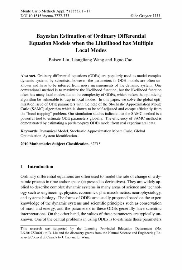
Figure 1. The experimental measurements for the concentrations of Chlorella andBrachionus in the predator-prey dynamic system when the dilution rate, δ = 0.65,and the inflow nitrogen concentration, N∗ = 80.

seven parameters, ε, α, m, bC , bB , kC , and kB in the above ODEs model all haveinteresting biological interpretations, but their values are unknown and need to beestimated from measurements of the dynamic system.

Figure 1 displays the experimental measurements for the concentrations of Chlorellaand Brachionus in the predator-prey dynamic system collected by [30] when thedilution rate, δ = 0.65, and the inflow nitrogen concentration, N∗ = 80. Bothpopulations of Chlorella and Brachionus show oscillation behavior, and it is inter-esting to estimate the parameters in the ODEs model (3.1) from these data. Noticethat we have no observations for two variables, the concentrations of nitrogen andreproducing Brachionus, in the ODEs model (3.1), which increases the challengefor parameter estimation.

Let β = log(ε, α,m, bC , bB, kC , kB)T be the logarithms of the vector of ODEparameters and α = log(N(t0), C(t0), R(t0), B(t0))

T be the logarithms of thevector of initial conditions of the ODEs model (3.1), where t0 is the startingtime point in the predator-prey experiment. Let Xi(t|θ), i = 1, . . . , 4, denotethe solution of the ODEs model (3.1) in the time domain [t0, tn], where θ =(αT ,βT ) is a vector of length 11, and denote θk, k = 1, . . . , 11, as the ele-ment of θ. Let y2j and y4j , j = 1, . . . , n, denote the measured concentrationsof Chlorella and Brachionus, respectively. We assume yij , i = 2, 4, is distributedwith N(Xi(tij |θ), σ2

i ). Then the log-likelihood function of θ and σ2 = (σ22, σ

24)

T

Estimating ODE Models 9

0.10.15

0.20.25

0.30.35

0.4

0.5

0.6

0.7

0.8

40

60

80

100

120

ε

m

50

60

70

80

90

100

110

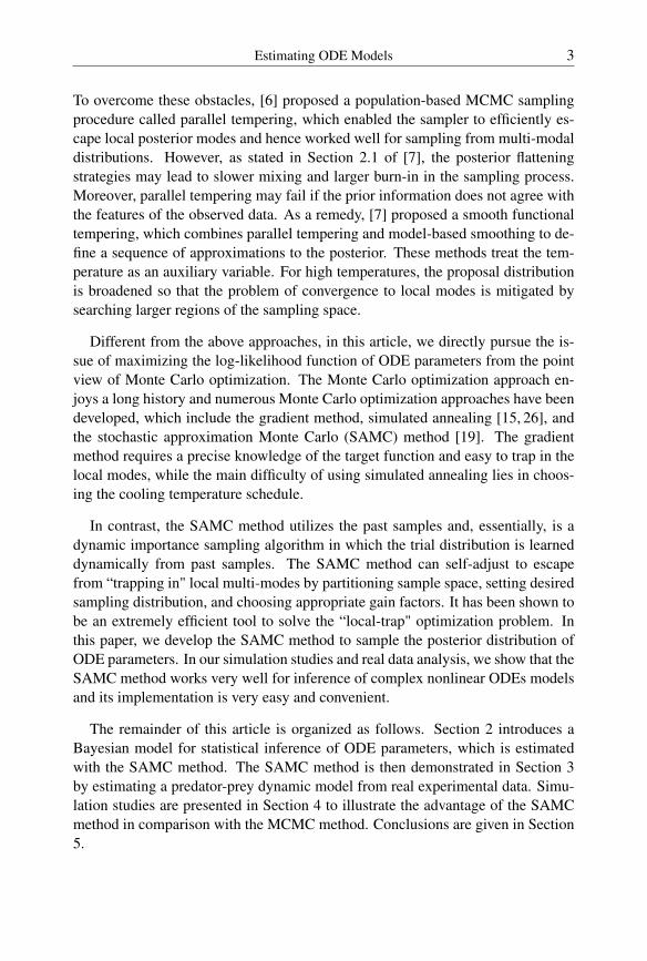
Figure 2. The surface of −U(θ) by varying the values of m and ε in [0.4,0.8] and[0.1,0.3] while setting other parameter values as estimates obtained in [8].

is given by

`(θ,σ2) = −∑i=2,4

n

2log(σ2

i )−12

∑i=2,4

σ−2i

n∑j=1

{yij −Xi(tij |θ)}2. (3.2)

Define U(θ) =∑

i=2,4∑n

j=1 wi{yij − Xi(tij |θ)}2 where the weights wi =

1/var(yi), yi = (yi1, . . . , yin)T for i = 2, 4. Figure 2 displays the surface of

−U(θ) by varying the values of m and ε in [0.4,0.8] and [0.1,0.3], respectively,while setting other parameter values as estimates obtained in [8]. It can be seenthat the surface of −U(θ) has multiple local modes, and it is not easy to arrive atthe global mode using traditional optimization approaches.

Instead, we will develop the SAMC method to search the minimum of U(θ) inthis article. Let Θ be the sample space for the ODE parameters, which is parti-tioned according to the values of U(θ) into the following subregions: E1 = {θ :

10 B. Liu, L. Wang and J. Cao

U(θ) < u1}, E2 = {θ : u1 ≤ U(θ) < u2}, . . . , and Em = {θ : U(θ) > um−1}with an equal bandwidth where u1 and um−1 are pre-specified real numbers. Weset u1 = 20 and um−1 = 36 with m = 50 and T0 defined in (2.6) is set asT0 = 5, 000.

After burning in the first 105 iterations, the SAMC method is continued to runfor 105 iterations. Table 1 displays the summary of SAMC estimation for theseven parameters in the ODEs model (3.1). The mean and standard deviation ofposterior samples are used as the parameter estimates and standard errors with theSAMC method, respectively. The parameter estimates with the SAMC methodis consistent to the generalized profiling estimates obtained in [8]. On the otherhand, the SAMC method has larger standard errors for parameter estimates thanthe generalized profiling method, because the latter are given for a fixed valueof the smoothing parameter. The SAMC method can also easily provide the 95%posterior credible intervals for the ODE parameter estimates based on the posteriorsampling sequence, which is the most appealing feature of the SAMC method incomparison with the generalized profiling method.

Table 1. The summary of Bayesian estimation for the seven parameters in the ODEsmodel (3.1). C.I. denotes the posterior credible interval of the ODE parameters.

Estimates Standard Errors 95% C.I.

ε 0.192 0.015 (0.162, 0.222)α 0.796 0.022 (0.753, 0.838)m 0.459 0.027 (0.406, 0.513)bC 3.876 0.404 (3.084, 4.667)bB 4.72 0.323 (4.083, 5.372)κC 7.065 1.778 (3.579, 10.550)κB 28.461 4.173 (20.282, 36.640)

4 Simulation

A simulation study is implemented to illustrate the advantage of the SAMC methodin comparison with the Metropolis-Hastings method when estimating parametersin an ODEs model from the noisy measurements of the dynamic system.

[16] introduced a mathematical model that was able to simulate physiological

Estimating ODE Models 11

oscillation on the basis of a negative feedback in cellular systems such as circadianrhythms and enzymatic regulation. A simple Goodwin model can be expressed inform of a set of ODEs

dX1(t)

dt=

7236 +X2(t)

− κ1,

dX2(t)

dt= κ2X1(t)− 1,

(4.1)

where X1(t) and X2(t) are the levels of mRNA and protein in the system, respec-tively. The parameter κ1 is the degradation rate constant, and κ2 is the synthesisrate constant.

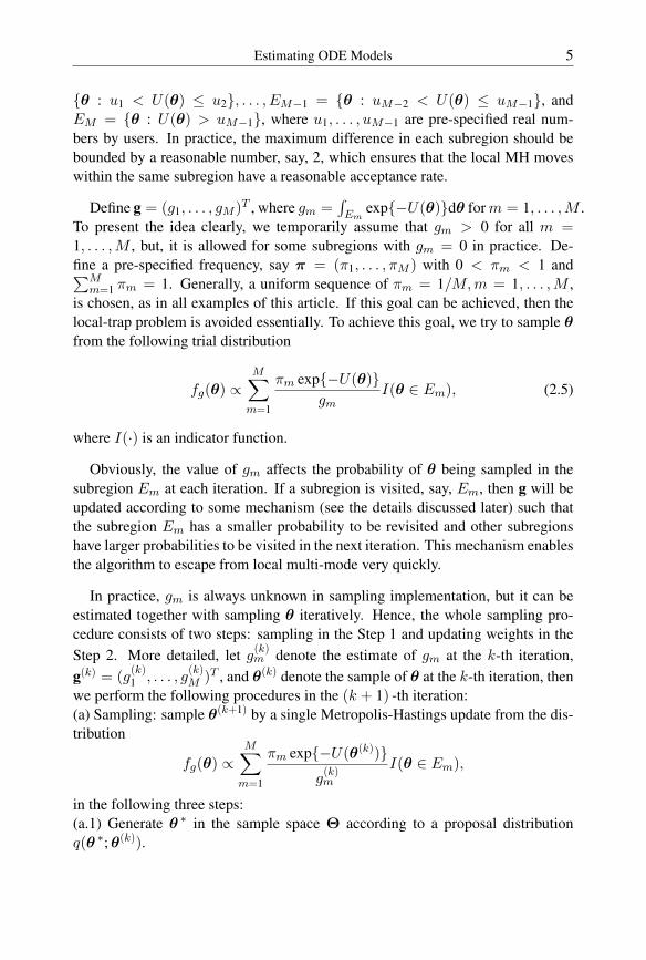
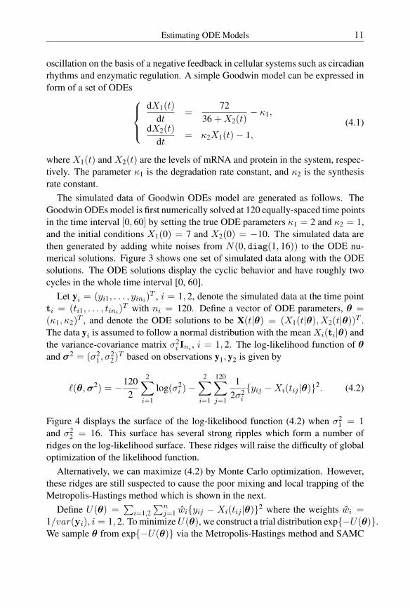
The simulated data of Goodwin ODEs model are generated as follows. TheGoodwin ODEs model is first numerically solved at 120 equally-spaced time pointsin the time interval [0, 60] by setting the true ODE parameters κ1 = 2 and κ2 = 1,and the initial conditions X1(0) = 7 and X2(0) = −10. The simulated data arethen generated by adding white noises from N(0, diag(1, 16)) to the ODE nu-merical solutions. Figure 3 shows one set of simulated data along with the ODEsolutions. The ODE solutions display the cyclic behavior and have roughly twocycles in the whole time interval [0, 60].

Let yi = (yi1, . . . , yini)T , i = 1, 2, denote the simulated data at the time point

ti = (ti1, . . . , tini)T with ni = 120. Define a vector of ODE parameters, θ =

(κ1, κ2)T , and denote the ODE solutions to be X(t|θ) = (X1(t|θ), X2(t|θ))T .

The data yi is assumed to follow a normal distribution with the mean Xi(ti|θ) andthe variance-covariance matrix σ2

i Ini , i = 1, 2. The log-likelihood function of θand σ2 = (σ2

1, σ22)

T based on observations y1, y2 is given by

`(θ,σ2) = −1202

2∑i=1

log(σ2i )−

2∑i=1

120∑j=1

12σ2

i

{yij −Xi(tij |θ)}2. (4.2)

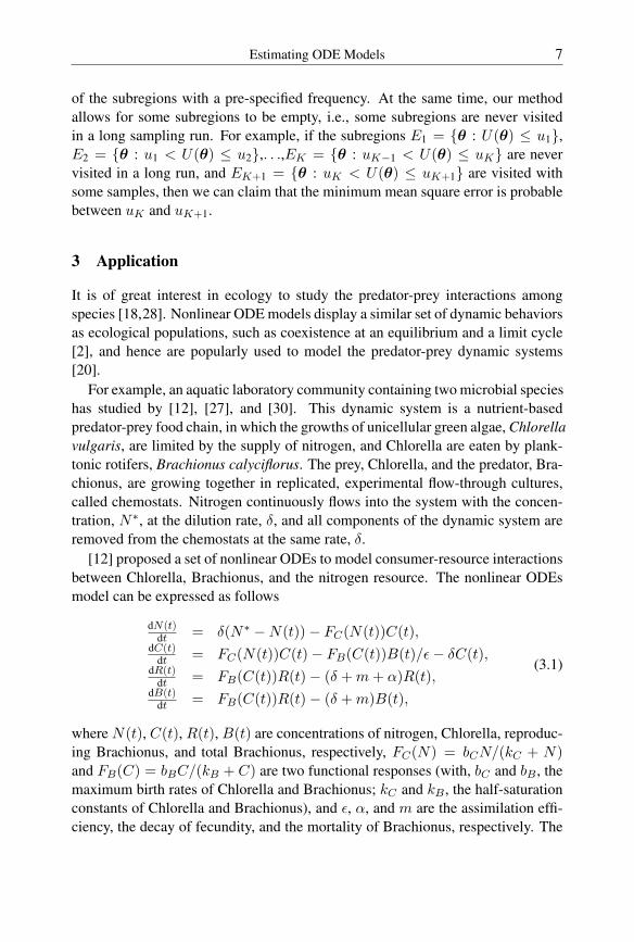
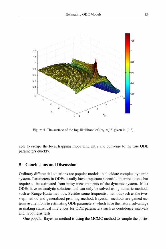
Figure 4 displays the surface of the log-likelihood function (4.2) when σ21 = 1

and σ22 = 16. This surface has several strong ripples which form a number of

ridges on the log-likelihood surface. These ridges will raise the difficulty of globaloptimization of the likelihood function.

Alternatively, we can maximize (4.2) by Monte Carlo optimization. However,these ridges are still suspected to cause the poor mixing and local trapping of theMetropolis-Hastings method which is shown in the next.

Define U(θ) =∑

i=1,2∑n

j=1 wi{yij − Xi(tij |θ)}2 where the weights wi =1/var(yi), i = 1, 2. To minimizeU(θ), we construct a trial distribution exp{−U(θ)}.We sample θ from exp{−U(θ)} via the Metropolis-Hastings method and SAMC

12 B. Liu, L. Wang and J. Cao

0 20 40 60−10

0

10

Time

X1(t

)

0 20 40 60−50

0

50

Time

X2(t

)

Figure 3. The data simulated by adding white noises to the numerical solutions ofthe Goodwin ODE (4.1). The solid lines are the ODE solutions by setting parameter,κ1 = 2 and κ2 = 1, and initial conditions X1(0) = 7, X2(0) = −10.

method, respectively.The Metropolis-Hastings method is used to sample 50,000 iterations for the two

ODE parameters (κ1, κ2)T based on the trial distribution exp{−U(θ)}, in which

the starting value of θ was randomly chosen. The sampling sequences for thetwo ODE parameters are displayed in the upper panels of Figure 5, which showsthat the sampling sequences are trapped at a local mode and are hard to convergeto the true parameter values. In contrast, the SAMC method is also applied tosampling 50,000 iterations for the two ODE parameters with the same startingvalue of θ using the same simulated data. Let Θ be the sample space for the twoODE parameters. We partition Θ according to the values of the objective function,U(θ), into the following subregions: E1 = {θ : U(θ) < u1}, E2 = {θ : u1 ≤U(θ) < u2}, . . . , and Em = {θ : U(θ) > um−1}, where u` = 7 + 0.592`,` = 1, . . . ,m, and m = 50. The sampling sequences for the two ODE parametersare displayed in the lower panels of Figure 5. It shows that the SAMC method is

Estimating ODE Models 13

0

1

2

3

4

5

0

1

2

3

4

5

6.2

6.4

6.6

6.8

7

7.2

7.4

κ2

κ1

6

6.2

6.4

6.6

6.8

7

7.2

Figure 4. The surface of the log-likelihood of (κ1, κ2)T given in (4.2).

able to escape the local trapping mode efficiently and converge to the true ODEparameters quickly.

5 Conclusions and Discussion

Ordinary differential equations are popular models to elucidate complex dynamicsystem. Parameters in ODEs usually have important scientific interpretations, butrequire to be estimated from noisy measurements of the dynamic system. MostODEs have no analytic solutions and can only be solved using numeric methodssuch as Runge-Kutta methods. Besides some frequentist methods such as the two-step method and generalized profiling method, Bayesian methods are gained ex-tensive attentions to estimating ODE parameters, which have the natural advantagein making statistical inferences for ODE parameters such as confidence intervalsand hypothesis tests.

One popular Bayesian method is using the MCMC method to sample the poste-

14 B. Liu, L. Wang and J. Cao

0 2 40

1

2

3

κ1

κ2

0 2 40

1

2

3

κ1

κ2

0 2 40

1

2

3

κ1

κ2

0 2 40

1

2

3

κ1

κ2

0 2 40

1

2

3

κ1

κ2

0 2 40

1

2

3

κ1

κ2

Figure 5. The sampling sequences for (κ1, κ2)T in the ODEs model (4.2) using the

Metropolis-Hastings method (upper panels) and the SAMC method (lower panels)with three starting values chosen randomly. The true values of the two ODE pa-rameters are κ1 = 2.0 and κ2 = 1.0, marked with circles. The panels from leftto right correspond to three starting values (marked with squares) of the two ODEparameters chosen randomly as: (3.1,2.4), (1.3,0.5), (0.2,0.5).

rior distribution of ODE parameters, which is easy to understand and implement.However, it is well known that the classical MCMC method is easy to be trappedin local modes of posterior distributions. Because ODE solutions are sensitive toODE parameters, the posterior distribution of ODE parameters often has manylocal modes. Therefore, the MCMC method is found to often be stuck in localmodes when sampling for ODE parameters.

In this paper, we suggest a Bayesian approach to solve the global optimizationproblem of the ODEs when the likelihood function has multiple local modes. Tosample the posterior distributions of ODE parameters, we develop the stochasticapproximation Monte Carlo (SAMC) method which is a self-adjusting mechanismand can update automatically the probabilities of subregions being visited in thesampling process. By performing numerical simulations, the advantage of the

Estimating ODE Models 15

SAMC method is illustrated, in which the SAMC method more efficiently escapesfrom local modes than the classical MCMC method. The SAMC method is alsodemonstrated by estimating a popular nutrient-based predator-prey dynamic modelfrom the experimental data.

Acknowledgments. We thank Prof. Gregor F. Fussmann for providing us thepredator-prey data set. The authors are also very grateful for the suggestions ofProf. Faming Liang.

Bibliography

[1] Y. Bard, Nonlinear parameter estimation., Academic Press, New York, 1974.

[2] L. Becks, F. M. Hilker, H. Malchow, K. Jürgens and H. Arndt, Experimental demon-stration of chaos in a microbial food web, Nature 435 (2005), 1226.

[3] L.T. Biegler, J. J. Damiano and G. E. Blau, Nonlinear Parameter Estimation: a CaseStudy Comparison, AIChE Journal 32 (1986), 29–45.

[4] N.J.B. Brunel, Parameter estimation of ODEs via nonparametric estimators, Elec-tronic Journal of Statistics 2 (2008), 1242–1267.

[5] J. C. Butcher, Numerical Methos for Ordinary Differential Equations, second ed,Wiley, Chichester, England, 2008.

[6] B. Calderhead and M. Girolami, Estimating Bayes factors via thermodynamic inte-gration and population MCMC, Computational Statistics & Data Analysis 53 (2009),4028–4045.

[7] D. Campbell and R. J. Steele, Smooth functional tempering for nonlinear differentialequation models, Statistics and Computing 22 (2012), 429–443.

[8] J. Cao, G.F. Fussmann and J. O. Ramsay, Estimating a predator-prey dynamicalmodel with the parameter cascades method, Biometrics 64 (2008), 959–967.

[9] J. Cao, J.Z. Huang and H. Wu, Penalized nonlinear least squares estimation of time-varying parameters in ordinary differential equations, Journal of computational andgraphical statistics 21 (2012), 42–56.

[10] J. Cao, L. Wang and J. Xu, Robust Estimation for Ordinary Differential EquationModels, Biometrics 67 (2011), 1305–1313.

[11] J. Chen and H. Wu, Efficient local estimation for time-varying coefficients in de-terministic dynamic models with applications to HIV-1 dynamics, Journal of theAmerican Statistical Association 103 (2008), 369–383.

[12] G. F. Fussmann, S. P. Ellner, K. W. Shertzer and N. G. Jr. Hairston, Crossing theHopf Bifurcation in a Live Predator-Prey System, Science 290 (2000), 1358–1360.

16 B. Liu, L. Wang and J. Cao

[13] A. Gelman, F. Bois and J. Jiang, Physiological Pharmacokinetic Analysis Using Pop-ulation Modeling and Informative Prior Distributions, Journal of the American Sta-tistical Association 91 (1996), 1400–1412.

[14] A. Gelman, J. B. Carlin, H.S. Stern and D. B. Rubin, Bayesian Data Analysis, Chap-man and Hall/CRC, New York, 2004.

[15] C.J. Geyer, Estimation and optimization of functions, Markov Chain Monte Carlo inPractice (W.R. Gilks, S. Richardson and D.J. Spiegelhalter, eds.), Chapman & Hall,London, 1996, pp. 241–258.

[16] B. Goodwin, Oscillatory behavior in enzymatic control processes, Adv. EnzymeRegul. 3 (1965), 425–438.

[17] Y. Huang, D. Liu and H. Wu, Hierachical Bayesian Methods for Estimation of Pa-rameters in a Longitudinal HIV Dynamic System, Biometrics 62 (2006), 413–423.

[18] B. E. Kendall, C. J. Briggs, W. W. Murdoch, P. Turchin, S. P. Ellner, E. McCauley,R. M. Nisbet and S. N. Wood, Why do populations cycle? A synthesis of statisticaland mechanistic modeling approaches, Ecology 80 (1999), 1789–1805.

[19] F. Liang, C. Liu and R. Carroll, Stochastic approximation in monte carlo computa-tion, Journal of the American Statistical Association 102 (2007), 305–320.

[20] W.W. Murdoch, C.J. Briggs and R.M. Nisbet, Consumer-Resource Dynamics,Princeton University Press, New York, 2003.

[21] A. Poyton, Application of principal differential analysis to parameter estimationin fundamental dynamics models, Master’s thesis, Queen’s University, Kingston,Canada, 2005.

[22] X. Qi and H. Zhao, Asymptotic efficiency and finite-sample properties of the gen-eralized profiling estimation of parameters in ordinary differ- ential equations, TheAnnals of Statistics 38 (2010), 435–481.

[23] J. O. Ramsay, G. Hooker, D. Campbell and J. Cao, Parameter estimation for differ-ential equations: a generalized smoothing approach (with discussion), Journal of theRoyal Statistical Society, Series B 69 (2007), 741–796.

[24] J. O. Ramsay and B. W. Silverman, Functional Data Analysis, second ed, Springer,New York, 2005.

[25] H. Robbins and S. Monro, A stochastic approximation method, The Annals of Math-ematical Statistics 22 (1951), 400–407.

[26] C. Robert and G. Casella, Monte Carlo Statistical Methods, second ed, Springer,New York, 2005.

[27] K. W. Shertzer, S. P. Ellner, G. F. Fussmann and N. G. Hairston, Predator-prey cy-cles in an aquatic microcosm: testing hypotheses of mechanism, Journal Of AnimalEcology 71 (2002), 802–815.

Estimating ODE Models 17

[28] P. Turchin, Complex population dynamics, Princeton University Press, Princeton,2003.

[29] J. M. Varah, A spline least squares method for numerical parameter estimation indifferential equations, SIAM Journal on Scientific Computing 3 (1982), 28 – 46.

[30] T. Yoshida, L. E. Jones, S. P. Ellner, G. F. Fussmann and N. G. Hairston, Rapidevolution drives ecological dynamics in a predator-prey system, Nature 424 (2003),303–306.

Received November 15, 2017.

Author information

Baisen Liu, School of Statistics, Dongbei University of Finance and Economics,Dalian,116025, China.E-mail: [email protected]

Liangliang Wang, Department of Statistics and Actuarial Science, Simon FraserUniversity, Burnaby, V5A1S6, Canada.E-mail: [email protected]

Jiguo Cao , Department of Statistics and Actuarial Science, Simon Fraser University,Burnaby, V5A1S6, Canada.E-mail: [email protected]