Bayesian Estimation of DSGE Models - · PDF fileBayesian paradigm (motivations) • Bayesian estimation of DSGE models with Dynare. 1. Data are not informative enough... 2. DSGE models

Bayesian Estimation of DSGE Models

Stéphane Adjemian

Université du Maine, GAINS & CEPREMAP

[email protected]

http://www.dynare.org/stepan

June 28, 2011

June 28, 2011 Université du Maine, GAINS & CEPREMAP Page 1

Bayesian paradigm (motivations)

• Bayesian estimation of DSGE models with Dynare.

1. Data are not informative enough...

2. DSGE models are misspecified.

3. Model comparison.

• Prior elicitation.

• Efficiency issues.


Bayesian paradigm (basics)

• A model defines a joint probability distribution

parametrized function over a sample of variables:

p(Y⋆T |θ) (1)

⇒ Likelihood.

• We Assume that our prior information about parameters

can be summarized by a joint probability density function.

Let the prior density be p0(θ).

• The posterior distribution is given by (Bayes theorem

squared):

p1 (θ|Y⋆T ) =

p0 (θ) p(Y⋆T |θ)

p(Y⋆T )

(2)


Bayesian paradigm (basics, contd)

• The denominator is defined by

p (Y⋆T ) =

∫

Θp0 (θ) p(Y

⋆T |θ)dθ (3)

⇒ the marginal density of the sample.

⇒ A weighted mean of the sample conditional densities

over all the possible values for the parameters.

• The posterior density is proportional to the product of the

prior density and the density of the sample.

p1 (θ|Y⋆T ) ∝ p0 (θ) p(Y

⋆T |θ)

⇒ That’s all we need for any inference about θ!

• The prior density deforms the shape of the likelihood!


A simple example (I)

• Data Generating Process

yt = µ+ εt

where εt ∼iid

N (0, 1) is a gaussian white noise.

• Let YT ≡ (y1, . . . , yT ). The likelihood is given by:

p(YT |µ) = (2π)−T2 e−

12

∑Tt=1(yt−µ)2

• And the ML estimator of µ is:

µML,T =1

T

T∑

t=1

yt ≡ y


A simple example (II)

• Note that the variance of this estimator is a simple function

of the sample size

V[µML,T ] =1

T

• Noting that:

T∑

t=1

(yt − µ)2 = νs2 + T (µ− µ)2

with ν = T − 1 and s2 = (T − 1)−1∑T

t=1(yt − µ)2.

• The likelihood can be equivalently written as:

p(YT |µ) = (2π)−T2 e−

12(νs

2+T (µ−µ)2)

The two statistics s2 and µ are summing up the sample

information.


A simple example (II, bis)

T∑

t=1

(yt − µ)2 =

T∑

t=1

([yt − µ]− [µ− µ])2

=T∑

t=1

(yt − µ)2 +T∑

t=1

(µ− µ)2 −T∑

t=1

(yt − µ)(µ− µ)

= νs2 + T (µ− µ)2 −

(T∑

t=1

yt − T µ

)(µ− µ)

= νs2 + T (µ− µ)2

The last term cancels out by definition of the sample mean.


A simple example (III)

• Let our prior be a gaussian distribution with expectation

µ0 and variance σ2µ.

• The posterior density is defined, up to a constant, by:

p (µ|YT ) ∝ (2πσ2µ)−

12 e

−12

(µ−µ0)2

σ2µ × (2π)−T2 e−

12(νs

2+T (µ−µ)2)

where the missing constant (denominator) is the marginal

density (does not depend on µ).

• We also have:

p(µ|YT ) ∝ exp

−1

2

(T (µ− µ)2 +

1

σ2µ(µ− µ0)

2

)


A simple example (IV)

A(µ) = T (µ− µ)2 +1

σ2µ

(µ− µ0)2

= T(µ2 + µ

2 − 2µµ)+

1

σ2µ

(µ2 + µ

20 − 2µµ0

)

=

(T +

1

σ2µ

)µ2 − 2µ

(T µ+

1

σ2µ

µ0

)+

(T µ

2 +1

σ2µ

µ20

)

=

(T +

1

σ2µ

)

µ2 − 2µT µ+ 1

σ2µ

µ0

T + 1σ2µ

+

(T µ

2 +1

σ2µ

µ20

)

=

(T +

1

σ2µ

)

µ−T µ+ 1

σ2µ

µ0

T + 1σ2µ

2

+

(T µ

2 +1

σ2µ

µ20

)

−

(T µ+ 1

σ2µ

µ0

)2

T + 1σ2µ


A simple example (V)

• Finally we have:

p(µ|YT ) ∝ exp

−

1

2

(T +

1

σ2µ

)[µ−

T µ+ 1σ2µµ0

T + 1σ2µ

]2

• Up to a constant, this is a gaussian density with (posterior)

expectation:

E [µ] =T µ+ 1

σ2µµ0

T + 1σ2µ

and (posterior) variance:

V [µ] =1

T + 1σ2µ


A simple example (VI, The bridge)

• The posterior mean is a convex combination of the prior

mean and the ML estimate.

– If σ2µ → ∞ (no prior information) then E[µ] → µ (ML).

– If σ2µ → 0 (calibration) then E[µ] → µ0.

• If σ2µ <∞ then the variance of the ML estimator is greater

than the posterior variance.

• Not so simple if the model is non linear in the estimated

parameters...

– Asymptotic (Gaussian) approximation.

– Simulation based approach (MCMC,

Metropolis-Hastings, ...).


Bayesian paradigm (II, Model Comparison)

• Comparison of marginal densities of the (same) data across

models.

• p(Y⋆T |I) measures the fit of model I.

• Suppose we have a prior distribution over models A, B, ...:

p(A), p(B), ...

• Again, using the Bayes theorem we can compute the

posterior distribution over models:

p(I|Y⋆T ) =

p(I)p(Y⋆T |I)∑

Ip(I)p(Y⋆

T |I)


Estimation of DSGE models (I, Reduced form)

• Compute the steady state of the model (a system of non

linear recurrence equations.

• Compute linear approximation of the model.

• Solve the linearized model:

yt − y(θ)n×1

= T (θ)n×n

(yt−1 − y(θ))n×1

+R(θ)n×q

εtq×1

(4)

where n is the number of endogenous variables, q is the

number of structural innovations.

– The reduced form model is non linear w.r.t the deep

parameters.

– We do not observe all the endogenous variables.


Estimation of DSGE models (II, SSM)

• Let y⋆t be a subset of yt gathering p observed variables.

• To bring the model to the data, we use a state-space

representation:

y⋆t = Z (yt + y(θ))+ηt (5a)

yt = T (θ)yt−1 +R(θ)εt (5b)

where yt = yt − y(θ).

• Equation (5b) is the reduced form of the DSGE model.

⇒ state equation

• Equation (5a) selects a subset of the endogenous variables,

Z is a p× n matrix filled with zeros and ones.

⇒ measurement equation


Estimation of DSGE models (III, Likelihood) – a –

• Let Y⋆T = y⋆1 , y

⋆2 , . . . , y

⋆T be the sample.

• Let ψ be the vector of parameters to be estimated (θ, the

covariance matrices of ε and η).

• The likelihood, that is the density of Y⋆T conditionally on

the parameters, is given by:

L(ψ;Y⋆T ) = p (Y⋆

T |ψ) = p (y⋆0 |ψ)T∏

t=1

p(y⋆t |Y

⋆t−1, ψ

)(6)

• To evaluate the likelihood we need to specify the marginal

density p (y⋆0 |ψ) (or p (y0|ψ)) and the conditional density

p(y⋆t |Y

⋆t−1, ψ

).


Estimation of DSGE models (III, Likelihood) – b –

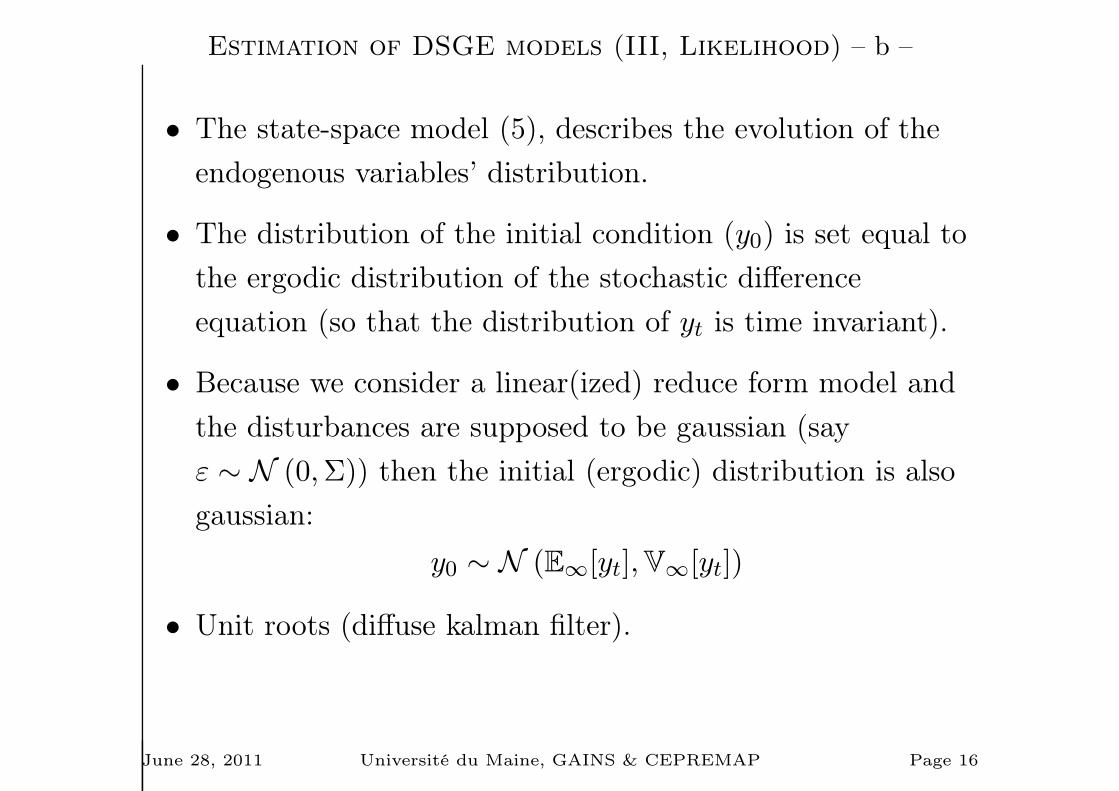
• The state-space model (5), describes the evolution of the

endogenous variables’ distribution.

• The distribution of the initial condition (y0) is set equal to

the ergodic distribution of the stochastic difference

equation (so that the distribution of yt is time invariant).

• Because we consider a linear(ized) reduce form model and

the disturbances are supposed to be gaussian (say

ε ∼ N (0,Σ)) then the initial (ergodic) distribution is also

gaussian:

y0 ∼ N (E∞[yt],V∞[yt])

• Unit roots (diffuse kalman filter).


Estimation (III, Likelihood) – c –

• Evaluation of the density of y⋆t |Y⋆t−1 is not trivial, because

y⋆t also depends on unobserved endogenous variables.

• The following identity can be used:

p(y⋆t |Y

⋆t−1, ψ

)=

∫

Λp (y⋆t |yt, ψ) p(yt|Y

⋆t−1, ψ)dyt (7)

The density of y⋆t |Y⋆t−1 is the mean of the density of y⋆t |yt

weigthed by the density of yt|Y⋆t−1.

• The first conditional density is given by the measurement

equation (5a).

• A Kalman filter is used to evaluate the density of the latent

variables (yt) conditional on the sample up to time t− 1

(Y⋆t−1) [⇒ predictive density ].


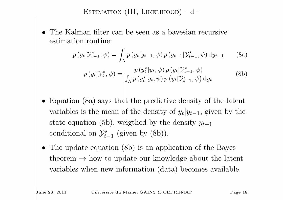
Estimation (III, Likelihood) – d –

• The Kalman filter can be seen as a bayesian recursiveestimation routine:

p (yt|Y⋆t−1, ψ) =

∫

Λ

p (yt|yt−1, ψ) p (yt−1|Y⋆t−1, ψ) dyt−1 (8a)

p (yt|Y⋆t , ψ) =

p (y⋆t |yt, ψ) p (yt|Y⋆t−1, ψ)∫

Λp (y⋆t |yt, ψ) p

(yt|Y⋆t−1, ψ

)dyt

(8b)

• Equation (8a) says that the predictive density of the latent

variables is the mean of the density of yt|yt−1, given by the

state equation (5b), weigthed by the density yt−1

conditional on Y⋆t−1 (given by (8b)).

• The update equation (8b) is an application of the Bayes

theorem → how to update our knowledge about the latent

variables when new information (data) becomes available.


Estimation (III, Likelihood) – e –

p (yt|Y⋆t , ψ) =

p (y⋆t |yt, ψ) p(yt|Y

⋆t−1, ψ

)∫Λ p (y

⋆t |yt, ψ) p

(yt|Y⋆

t−1, ψ)dyt

• p(yt|Y⋆

t−1, ψ)

is the a priori density of the latent variables

at time t.

• p (y⋆t |yt, ψ) is the density of the observation at time t

knowing the state and the parameters (this density is

obtained from the measurement equation (5a)) ⇒ the

likelihood associated to y⋆t .

•∫Λ p (y

∗t |yt, ψ) p

(yt|Y⋆

t−1, ψ)dyt is the marginal density of

the new information.


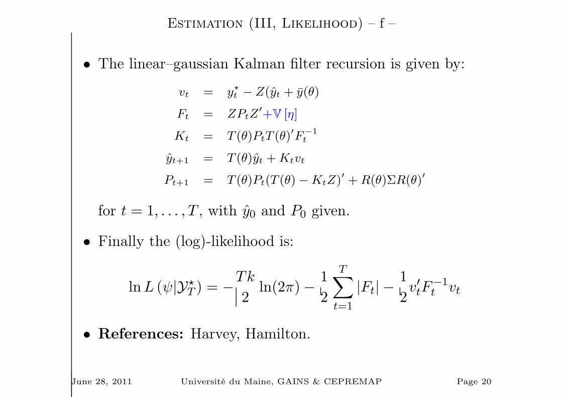
Estimation (III, Likelihood) – f –

• The linear–gaussian Kalman filter recursion is given by:

vt = y⋆t − Z(yt + y(θ)

Ft = ZPtZ′+V [η]

Kt = T (θ)PtT (θ)′

F−1t

yt+1 = T (θ)yt +Ktvt

Pt+1 = T (θ)Pt(T (θ)−KtZ)′ + R(θ)ΣR(θ)′

for t = 1, . . . , T , with y0 and P0 given.

• Finally the (log)-likelihood is:

lnL (ψ|Y⋆T ) = −

Tk

2ln(2π)−

1

2

T∑

t=1

|Ft| −1

2v′tF

−1t vt

• References: Harvey, Hamilton.


Simulations for exact posterior analysis

• Noting that:

E [ϕ(ψ)] =

∫

Ψϕ(ψ)p1(ψ|Y

⋆T )dψ

we can use the empirical mean of(ϕ(ψ(1)), ϕ(ψ(2)), . . . , ϕ(ψ(n))

), where ψ(i) are draws from

the posterior distribution to evaluate the expectation of

ϕ(ψ). The approximation error goes to zero when n→ ∞.

• We need to simulate draws from the posterior distribution

⇒ Metropolis-Hastings.

• We build a stochastic recurrence whose limiting

distribution is the posterior distribution.


Simulations (Metropolis-Hastings) – a –

1. Choose a starting point Ψ0 & run a loop over 2-3-4.

2. Draw a proposal Ψ⋆ from a jumping distribution

J(Ψ⋆|Ψt−1) = N (Ψt−1, c× Ωm)

3. Compute the acceptance ratio

r =p1(Ψ

⋆|Y⋆T )

p(Ψt−1|Y⋆T )

=K(Ψ⋆|Y⋆

T )

K(Ψt−1|Y⋆T )

4. Finally

Ψt =

Ψ⋆ with probability min(r, 1)

Ψt−1 otherwise.


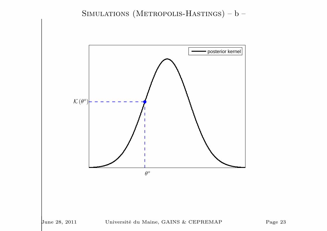
Simulations (Metropolis-Hastings) – b –

θo

K (θo)

posterior kernel


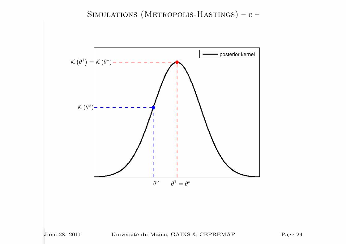
Simulations (Metropolis-Hastings) – c –

θo

K (θo)

θ1 = θ

∗

K(

θ1)

= K (θ∗)

posterior kernel


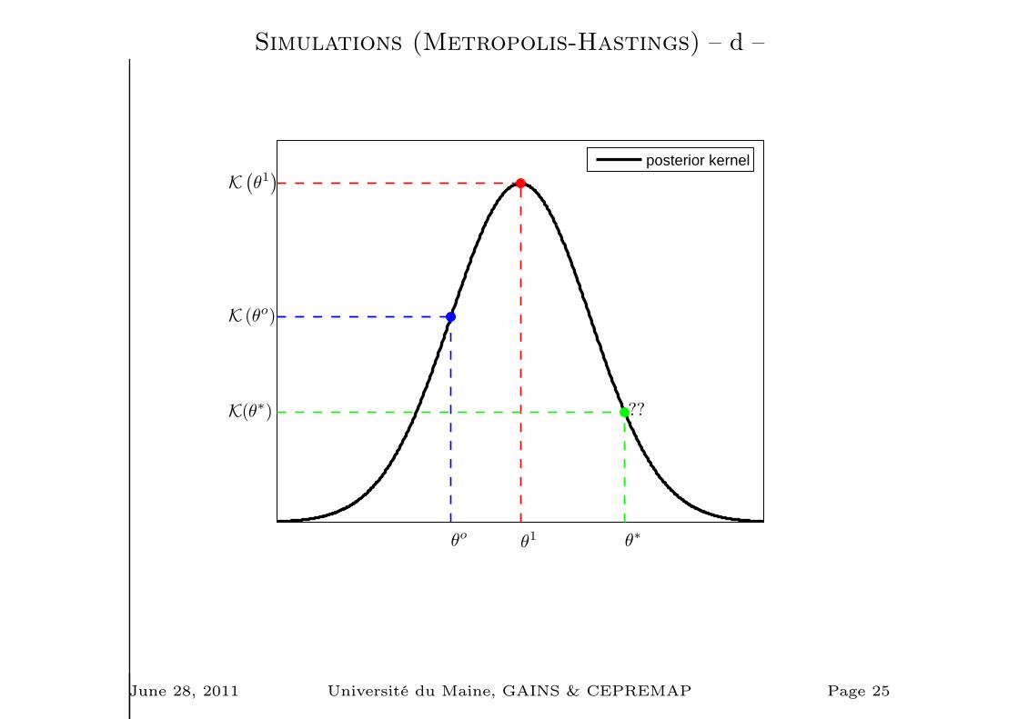
Simulations (Metropolis-Hastings) – d –

θo

K (θo)

θ1

K(

θ1)

θ∗

K(θ∗) ??

posterior kernel


Simulations (Metropolis-Hastings) – e –

• How should we choose the scale factor c (variance of the

jumping distribution) ?

• The acceptance rate should be strictly positive and not too

important.

• How many draws ?

• Convergence has to be assessed...

• Parallel Markov chains → Pooled moments have to be

close to Within moments.


Dynare syntax (I)

var A B C;

varexo E;

parameters a b c d e f ;

model(linear);

A=A(+1)-b/e*(B-C(+1)+A(+1)-A);

C=f*A+(1-d)*C(-1);

....

end;


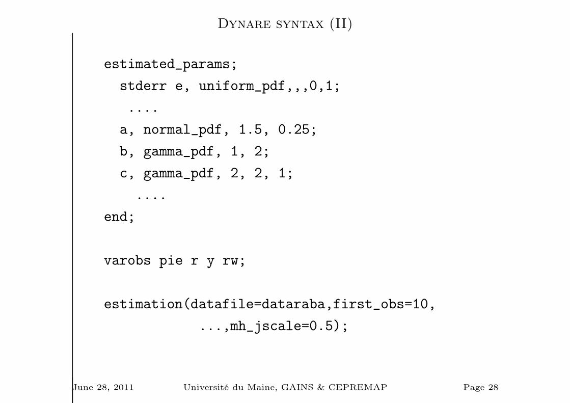
Dynare syntax (II)

estimated_params;

stderr e, uniform_pdf,,,0,1;

....

a, normal_pdf, 1.5, 0.25;

b, gamma_pdf, 1, 2;

c, gamma_pdf, 2, 2, 1;

....

end;

varobs pie r y rw;

estimation(datafile=dataraba,first_obs=10,

...,mh_jscale=0.5);


Prior Elicitation

• The results may depend heavily on our choice for the prior

density or the parametrization of the model (not

asymptotically).

• How to choose the prior ?

– Subjective choice (data driven or theoretical), example:

the Calvo parameter for the Phillips curve.

– Objective choice, examples: the (optimized)

Minnesota prior for VAR (Phillips, 1996).

• Robustness of the results must be evaluated:

– Try different parametrization.

– Use more general prior densities.

– Uninformative priors.


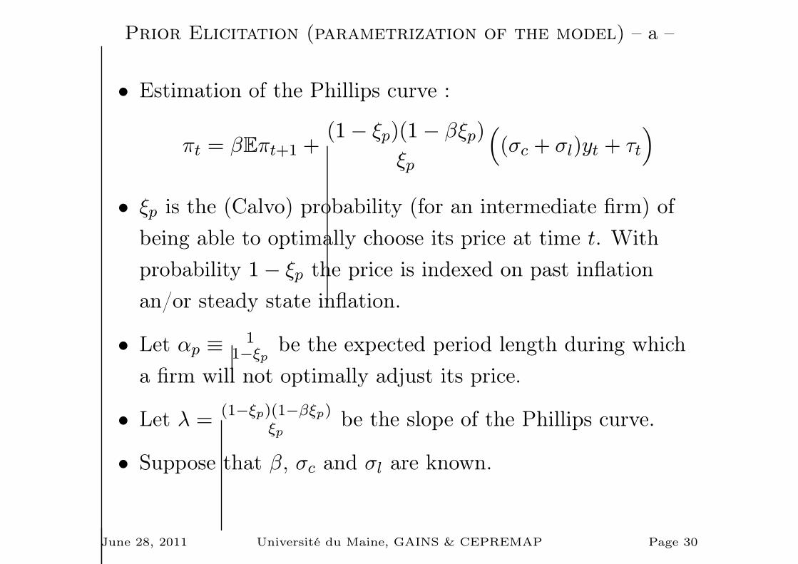
Prior Elicitation (parametrization of the model) – a –

• Estimation of the Phillips curve :

πt = βEπt+1 +(1− ξp)(1− βξp)

ξp

((σc + σl)yt + τt

)

• ξp is the (Calvo) probability (for an intermediate firm) of

being able to optimally choose its price at time t. With

probability 1− ξp the price is indexed on past inflation

an/or steady state inflation.

• Let αp ≡1

1−ξpbe the expected period length during which

a firm will not optimally adjust its price.

• Let λ =(1−ξp)(1−βξp)

ξpbe the slope of the Phillips curve.

• Suppose that β, σc and σl are known.


Prior Elicitation (parametrization of the model) – b –

• The prior may be defined on ξp, αp or the slope λ.

• Say we choose a uniform prior for the Calvo probability:

ξp ∼ U[.51,.99]

The prior mean is .75 (so that the implied value for αp is 4

quarters). This prior is often think as a non informative

prior...

• An alternative would be to choose a uniform prior for αp:

αp ∼ U[1− 1.51

,1− 1.99 ]

• These two priors are very different!


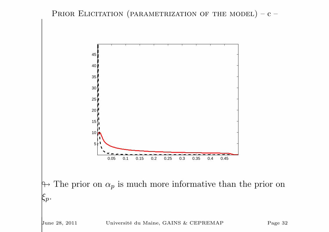
Prior Elicitation (parametrization of the model) – c –

0.05 0.1 0.15 0.2 0.25 0.3 0.35 0.4 0.45

5

10

15

20

25

30

35

40

45

# The prior on αp is much more informative than the prior on

ξp.


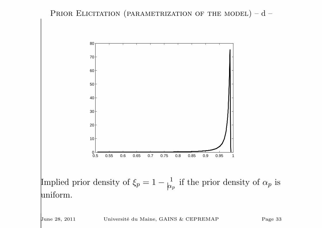
Prior Elicitation (parametrization of the model) – d –

0.5 0.55 0.6 0.65 0.7 0.75 0.8 0.85 0.9 0.95 10

10

20

30

40

50

60

70

80

Implied prior density of ξp = 1− 1αp

if the prior density of αp is

uniform.


Prior Elicitation (more general prior densities)

• Robustness of the results may be evaluated by considering

a more general prior density.

• For instance, in our simple example we could assume a

student prior density for µ instead of a gaussian density.


Prior Elicitation (flat prior)

• If a parameter, say µ, can take values between −∞ and ∞,

the flat prior is a uniform density between −∞ and ∞.

• If a parameter, say σ, can take values between 0 and ∞, the

flat prior is a uniform density between −∞ and ∞ for log σ:

p0(log σ) ∝ 1 ⇔ p0(σ) ∝1

σ

• Invariance.

• Why is this prior non informative ?...∫p0(µ)dµ is not

defined! ⇒ Improper prior.

• Practical implications for DSGE estimation.


Prior Elicitation (non informative prior)

• An alternative, proposed by Jeffrey, is to use the Fisher

information matrix:

p0(ψ) ∝ |I(ψ)|12

with

I(ψ) = E

[(∂p(Y⋆

T |ψ)

∂ψ

)(∂p(Y⋆

T |ψ)

∂ψ

)′]

• The idea is to mimic the information in the data...

• Automatic choice of the prior.

• Invariance to any continuous transformation of the

parameters.

• Very different results (compared to the flat prior) ⇒ Unit

root controverse.


Effective prior mass

• Dynare excludes parameters such that the steady state does

not exist, or such that the BK conditions are not satisfied.

• The effective prior mass can be less than 1.

• Comparison of marginal densities of the data is not

informative if the prior mass is not invariant across models.

• The estimation of the posterior mode is more difficult if the

effective prior mass is less than 1.


Efficiency (I)

• If possible use options use_dll (need a compiler, gcc)

• Do not let dynare compute the steady state!

• Even if there is no closed form solution for the steady state,

the static model can be concentrated and reduced to a

small nonlinear system of equations, which can be solved by

using standard newton algorithm in the steastate file.

This numerical part can be done in a mex routine called by

the steastate file.

• Alternative initialization of the Kalman filter (lik_init=4).


Efficiency (II)

Fixed point of the state equation Fixed point of the Riccati equation

Execution time 7.28 3.31

Likelihood -1339.034 -1338.915

Marginal density 1296.336 1296.203

α 0.3526 0.3527

β 0.9937 0.9937

γa 0.0039 0.0039

γm 1.0118 1.0118

ρ 0.6769 0.6738

ψ 0.6508 0.6508

δ 0.0087 0.0087

σεa 0.0146 0.0146

σεm 0.0043 0.0043

Table 1: Estimation of fs2000. In percentage the maximum

deviation is less than 0.45.


Bayesian Estimation of DSGE Models - · PDF fileBayesian paradigm (motivations) • Bayesian estimation of DSGE models with Dynare. 1. Data are not informative enough... 2. DSGE models

Documents