Bayesian Causal Inference Under Conditional Ignorability * Siddhartha Chib † July 2017 Abstract In this paper we describe a Bayesian approach for finding the causal effect with observa- tional data under the assumption that the binary treatment variable is conditionally ignor- able. In our approach, the potential outcome distributions are modeled directly through spline-based (basis function) regression techniques and the relevant potential outcome dis- tributions are estimated separately from the data on the control and treated subjects. An important facet of the approach is that the average treatment effect (ATE) is calculated from a predictive perspective (post estimation) in which the missing outcomes of the control subjects are predicted from the model of the treated subjects while the missing outcomes of the treated subjects are predicted from the model of the control subjects. We show that this strategy works, even with covariate imbalance, if the knots in the basis expansions are chosen in a specific way from the combined covariate values of both the control and treated subjects. We illustrate the performance of our approach against frequentist matching-type estimators using both simulated and real data. Key words : Average treatment effect; cubic spline; Markov chain Monte Carlo; marginal likelihood; observational data; overlap problem; semiparametric Bayesian inference. 1 Introduction In the context of observational (non-experimental) data, suppose that x ∈{0, 1} is a binary treatment variable and let z denote a k-dimensional vector of observed pre-treatment covariates or confounder (control) variables. Suppose that the treatment intake mechanism is described by the probability model Pr(x =1|z)= e(z) and that this probability (called the propensity score) satisfies the overlap condition 0 <e(z) < 1, for all z. Also let y 0 and y 1 denote the potential outcomes, and suppose that the treatment is conditionally ignorable, i.e., independent of the potential outcomes given the confounders. Then, the ATE, given by the difference E(y 1 )-E(y 0 ), * Thanks to Dr. Sandor Kovacs of the Washington University School of Medicine for explaining the right heart catherization procedure, and to participants at seminars at Yale University (April 2010) and University of Melbourne (2014). This paper is dedicated to the memory of Edward Greenberg, friend and collaborator, whose explorations and development of the Bayesian viewpoint over several decades have left a rich legacy. † Olin Business School, Washington University in St. Louis, St. Louis MO 63130; [email protected]

Welcome message from author
This document is posted to help you gain knowledge. Please leave a comment to let me know what you think about it! Share it to your friends and learn new things together.
Transcript
Bayesian Causal Inference Under Conditional
Ignorability∗
Siddhartha Chib†
July 2017
Abstract
In this paper we describe a Bayesian approach for finding the causal effect with observa-tional data under the assumption that the binary treatment variable is conditionally ignor-able. In our approach, the potential outcome distributions are modeled directly throughspline-based (basis function) regression techniques and the relevant potential outcome dis-tributions are estimated separately from the data on the control and treated subjects. Animportant facet of the approach is that the average treatment effect (ATE) is calculatedfrom a predictive perspective (post estimation) in which the missing outcomes of the controlsubjects are predicted from the model of the treated subjects while the missing outcomesof the treated subjects are predicted from the model of the control subjects. We show thatthis strategy works, even with covariate imbalance, if the knots in the basis expansions arechosen in a specific way from the combined covariate values of both the control and treatedsubjects. We illustrate the performance of our approach against frequentist matching-typeestimators using both simulated and real data.
Key words: Average treatment effect; cubic spline; Markov chain Monte Carlo; marginallikelihood; observational data; overlap problem; semiparametric Bayesian inference.
1 Introduction
In the context of observational (non-experimental) data, suppose that x ∈ {0, 1} is a binary
treatment variable and let z denote a k-dimensional vector of observed pre-treatment covariates
or confounder (control) variables. Suppose that the treatment intake mechanism is described by
the probability model Pr(x = 1|z) = e(z) and that this probability (called the propensity score)
satisfies the overlap condition 0 < e(z) < 1, for all z. Also let y0 and y1 denote the potential
outcomes, and suppose that the treatment is conditionally ignorable, i.e., independent of the
potential outcomes given the confounders. Then, the ATE, given by the difference E(y1)−E(y0),
∗Thanks to Dr. Sandor Kovacs of the Washington University School of Medicine for explaining the rightheart catherization procedure, and to participants at seminars at Yale University (April 2010) and Universityof Melbourne (2014). This paper is dedicated to the memory of Edward Greenberg, friend and collaborator,whose explorations and development of the Bayesian viewpoint over several decades have left a rich legacy.†Olin Business School, Washington University in St. Louis, St. Louis MO 63130; [email protected]

where the expectations are with respect to the marginal distribution of the potential outcomes,
is identified. In this paper, we are interested in developing a Bayesian approach for estimating
the ATE under the overlap and conditional ignorability assumptions.
The ATE is commonly found by frequentist matching methods, such as the method of
propensity score matching (Rosenbaum and Rubin, 1983). In this method, the propensity
score is estimated by a flexible logit or probit model, and then two individuals with the same
propensity score, one treated and one control, are matched. The difference in outcomes of such
matched subjects is the average treatment effect (ATE) conditioned on the propensity score.
Averaging these differences across matched subjects leads to an estimate of the ATE.
It is not possible to develop a Bayesian approach that strictly parallels the frequentist
propensity score matching method. This is because propensity score matching is an algorithm
that cannot be described in likelihood terms. A more fundamental issue is that, under con-
ditional ignorability, the treatment is independent of the outcomes and thus plays no role in
inferences about the potential outcome distributions. Nonetheless, attempts at formulating
causal inferences based on Bayesian versions of propensity scores are described in, for example,
Hoshino (2008), An (2010), Kaplan and Chen (2012) and Zigler et al. (2013). In this paper we
pursue an alternative approach from the Bayesian side which is to model the potential outcome
distributions directly and to estimate the y0 distribution from the control subjects and the y1
distribution from the treated subjects. In this modeling we use spline-based (basis function)
regression techniques to non-parametrically model the distributions of y0 and y1 given the
confounders. We do not need to estimate the unidentified joint distribution of (y0, y1) for each
subject, as this joint distribution is not required, following Chib (2007). We then estimate the
ATE by predicting y1 for the control subjects from the model of y1 estimated from the treated
subjects, and by predicting y0 for the treated subjects from the model of y0 estimated from
the control subjects. We show that this strategy works (even when the distribution of the
confounders is quite different for the control and treated subjects - the problem of covariate
2

imbalance) if the knots in the basis expansions are chosen in a specific way from the com-
bined covariate values of both the control and treated, even while only the data on the control
subjects is used to estimate the y0 model and only the data on the treated subjects is used
to estimate the y1 model. When there is no overlap in the covariate distributions across the
treatment and control subjects, our approach would fail, as would those based on matching
methods, but as long as the overlap condition holds, our approach for selecting knots leads
to accurate estimates of the ATE, as we show below. Our approach produces the posterior
distribution of the ATE, marginalized over parameter and model uncertainties.
Our approach assumes that the set of covariates z that produce conditional ignorability of
the treatment are known in advance. We do allow the set of available confounders to exceed
those in z. In that case, we judge the relevance of those additional confounders by comparing
the marginal likelihoods of the models with and without those additional confounders. We
calculate these marginal likelihoods by the method of Chib (1995).
Non-parametric modeling of the potential outcomes has also been considered by Hill (2011)
but from a Bayesian CART perspective. McCandless et al. (2009) considers a quite different
Bayesian approach for outcome modeling by letting the outcomes depend on the propensity
score. This requires the estimation of both the propensity score and outcome models and leads
to a complex estimation procedure. Joint modeling of outcome and treatment models with a
particular focus on the question of confounder choice is discussed in Wang et al. (2012) while
Saarela et al. (2016) provide an approach in which both models are estimated with the aim
of achieving robustness to confounder misspecification. Our approach in this paper is in some
sense complementary to these approaches because it explores the Bayesian analysis under the
assumption that conditional ignorability holds for the given set of confounders. An important
difference between Hill (2011) and our work is that we stress the issue of covariate imbalance
and propose a knot selection procedure to address it, but Hill does not discuss how the CART
approach would perform with significant covariate imbalance, as in one of the problems we
3

consider.
The rest of the paper is organized as follows. In Section 2 we present the approach for
outcome modeling along with our method for selecting knots for the cubic spline basis matrices.
The estimation of the models from the control and treated subject data is also described in this
section followed by our approach for calculating the posterior distribution of the ATE in Section
3. The application of the methodology is first illustrated in Section 4 with an example that
has considerable covariate imbalance and then with real data in Section 5. Section 6 contains
our conclusions. Appendix A explains the construction of the basis matrix, and Appendix B
presents details of our prior distribution.
2 Approach: outcome modeling and estimation
Let p0(y|z) and p1(y|z) denote the conditional distributions of y0 and y1 given the confounders.
These do not depend on x because of the conditional ignorability assumption. We model these
distributions in a semi-parametric way by combining a parametric student-t distribution for
pj (.) with additive non-parametric modeling of the covariate affects. In addition, suppose that
the vector of confounders is split into two components, z = (v, w1, ..., wq), where v : kv × 1 are
categorical predictors including the intercept, and {wr} are continuous predictors with non-
linear effects on the outcome. We suppose that the outcome distribution in the x = 0 state is
p0(y0|z) = tν0
(y0|v
′β00 + g01(w1) + · · ·+ g0q(wq), σ
20
)(2.1)
and in the x = 1 state is
p1(y1|z) = tν1
(y1|v
′β10 + g11(w1) + · · ·+ g1q(wq), σ
21
)(2.2)
where, for j = 0, 1, tνj is the student-t density with νj > 2 degrees of freedom, gjr (·) is an
unknown smooth function of wr for r ≤ q, and σ2j is the dispersion. The following remarks
are in order. The preceding specify the marginal distributions of the potential outcomes. The
unidentified joint distribution of (y0, y1) is not needed, following Chib (2007), because the
4

missing counterfactuals can be simply integrated out. Second, this modeling of the marginal
distributions is saturated in the sense that the mean, dispersion and degrees of freedom are
allowed to differ. Finally, the student-t assumption is important in practice. It provides
substantially improved models, especially when the mean function, as above, is modeled non-
parametrically. Further generality can be achieved, if desired, by putting a non-parametric
prior (such as the Dirichlet process) on these distributions.
2.1 Sample data
Suppose we have sample data (xi, yi,v′i,w′i) on n independently distributed subjects (i =
1, . . . , n), where yi = xiy1i + (1 − xi)y0i, organized so that the first n0 observations are those
for the controls (xi = 0) and the next n1 = n− n0 are for the treated (xi = 1):
xi = 0, y0i, y∗1i, yi = y0i, v′i,w′i, i = 1, . . . , n0, (2.3)
xi = 1, y∗0i, y1i, yi = y1i, v′i,w′i, i = n0 + 1, . . . , n, (2.4)
where a star indicates the missing counterfactual outcome. In vector notation, in the control
group, the observed outcome data are
y0 = (y01, . . . , y0n0) : n0 × 1
and the missing counterfactual outcomes are
y∗1c = (y∗11, . . . , y∗1n0
)
to be read as “y1 for the controls.” Similarly, in the treated group, the observed outcome data
are
y1 = (y1n0+1, . . . , y1n) : n1 × 1
and the missing counterfactual outcomes are the “y0 for the treated”
y∗0t = (y∗0n0+1, . . . , y∗0n)
5

The associated matrix of linear confounders, split by intake status, are indicated by
V0 = (v1, ...,vn0)′ : n0 × kv and V1 = (vn0+1, ...,vn)′ : n1 × kv
and those of the non-linear confounders by
W0 = (w1, ...,wn0)′ : n0 × q and W1 = (wn0+1, ...,wn)′ : n1 × q
In the sequel it will also be necessary to work with all n observations on the confounders in w,
in which case we write
W =
(W0
W1
)= (w.1,w.2, . . . ,w.q) (2.5)
where w.r (r ≤ q) denotes the rth column of W.
2.2 Knots and basis matrices
We now discuss the estimation of the p0(y0|z) model given the data on the control subjects
and of the p1(y1|z) given the data on the treated subjects. Then, the ATE is calculated
(post-estimation) from the predictions of y∗1c for the control subjects using the model p1(y1|z)
estimated on the treated subjects, and from the predictions of y∗0t for the treated subjects
using the model p0(y0|z) estimated on the control subjects.
To make this procedure concrete, we suppose that each gjr(wr) function is in the span
of the natural cubic splines. We use the basis from Chib and Greenberg (2010) and a prior
on the basis coefficients from Chib and Greenberg (2014) to do our prior-posterior analysis
on these functions. Since the ATE is calculated by a predictive approach, it is important to
recognize the potential problems that can arise from covariate imbalance across the two groups
of subjects. If the problem of covariate imbalance is extreme, no method can be expected to
work adequately. In the case of matching, the problem of extreme covariate imbalance would
manifest itself in the form of fewer matches. In our method, the problem would be revealed by
a more dispersed posterior distribution of the ATE.
The question now is how to develop a predictive approach that would work in other less
problematic cases of covariate imbalance. The key idea here is to estimate the p0(y0|z) and
6

p1(y1|z) models in such a way that accurate predictions of the counterfactuals are possible.
Our study of this problem reveals the key role played by the choice of knots. The default
strategy of equally spaced knots often turns to be unsatisfactory, even with moderate levels
of covariate imbalance across the two groups of subjects. In that case, equally spaced knots
based on (say) the control observations would miss some of the covariate values in the treated
group, which would lead to intervals in the control and treatment groups with no observations,
and instability of the spline basis matrices and inaccurate extrapolation of the spline estimated
from the control observations to those covariate values in the treated group.
Instead, we propose another strategy that overcomes the preceding problem. As motivation,
consider for example the function g0r(wr) in the control model. For estimating this function,
the outcome data available to us is just that from the n0 control subjects. But for purposes of
making the basis functions we have data on wr not just from the control subjects but also from
the treated subjects. One can take advantage of this additional data on wr for placing knots
and constructing the basis matrix. Having made the basis matrix from all n observations,
one simply drops the last n1 rows while estimating the control model. The remaining n1
basis matrix rows are used when predicting y∗0i for the treated. Similarly, we use all the n
observations on wr to make the basis matrix for the function g1r(wr) but then we remove the
first n0 rows of that basis matrix while estimating the outcome model of the treated subjects.
Those n0 rows are used in the prediction of y∗1i for the controls.
We now explain how this strategy is implemented. For a given covariate wr, suppose we
need to locate mjr knots. The notation mjr indicates that the number of knots for a given
covariate wr could vary by control and treated subjects. Consider now the entire data on wr,
namely (w1r, . . . , wnr). Let the first knot τ r1 be located at min(w1r, . . . , wnr) and the last knot
τ rmr at max(w1r, . . . , wnr). To find the remaining mjr − 2 knots, define
maxminr = max(min(w1r, . . . , wn0r),min(wn0+1r, . . . , wnr)),
minmaxr = min(max(w1r, . . . , wn0r),max(wn0+1r, . . . , wnr))
7

Now let ajr = (maxminr, ar2, . . . , ar,mjr−1,minmax) denote mjr evenly spaced values between
maxminr and minmaxr. Then, our set of mjr knots is given by the collection
τ r = (τ r1, ar2, . . . , ar,mjr−1, τ rmr ).
It can be checked that with this (novel) approach, even with covariate imbalance, use of these
knots ensures that the smallest and largest knots include the required interval for both the
control and treated observations and that there are no empty intervals between knots. If there
is no covariate imbalance or only minor imbalance, these knots will be very nearly evenly
spaced between the smallest and largest values of wr.
Given the knots, we express each of the gjr(w.r) functions at the n covariate values w.r by
a natural cubic spline. Applying the spline transformation given in Appendix A we have
g0r(w.r) = B0rβ0r , r = 1, 2, ..., q
and
g1r(w.r) = B1rβ1r , r = 1, 2, ..., q
where Bjr : n× (Mjr−1) is the basis matrix and βjr : (Mjr−1)×1 are the spline coefficients.
It is helpful to assemble these basis matrices in the following way. The basis matrices from
expanding the g0r(w.r) functions can be assembled as
Bc = (V,B01, . . . ,B0q)
starting with the matrix of linear covariates V = (V′0,V′1)′. Only the first n0 rows of Bc are
used in the estimation of the control model. Thus, it is further useful to partition Bc at row
n0 as
Bc =
(B0
B0t
)
where the matrix B0t is used for the prediction of the missing y∗0t for the treated subjects in
the sample.
8

Similarly, the basis matrices from expanding the g1r(w.r) functions can be assembled as
Bt = (L,B11, . . . ,B1q)
starting again with the matrix of linear covariates V. Because only the last n1 rows of Bt are
to be used in the estimation of the treatment model it is further useful to partition Bt at row
n0 as
Bt =
(B1c
B1
)
where the matrix B1c is used for the prediction of the missing y∗1c for the control subjects in
the sample.
2.3 Estimation of the control subject model
The model of the observed data on the control subjects after the basis function expansions can
now be expressed as
y0 = B0β0 + ε0, (2.6)
where B0 are the first n0 rows of Bc,
β0 =(β′00,β
′01, ...,β
′0r
)′: k0 × 1
is of size k0 = kv +q∑r=1
(m0r − 1), and ε0 is a n0 vector of independently distributed student-t
random variables with ν degrees of freedom and dispersion σ20.
Let ξ0 = (ξ01, . . . , ξ0n0) where
ξ0i ∼ G(ξ0i|
ν02,ν02
), i ≤ n0
denote the Gamma distributed mixing variables in the hierarchical representation of the student-
error error distribution
ε0i|ξ0i ∼ N (0, ξ−10i σ20)
Also let the prior take the form
π(β0|λ0)π(σ20)π(λ0)
9

where λ0 : (r + 1) × 1 is a vector of smoothness parameters, as detailed in Appendix B.
Then, the posterior distribution of (β0, σ20), augmented with (ξ0,λ0), and conditioned on the
given outcomes y0, the covariates in B0 and the degrees of freedom ν0 of the student-t error
distribution is
π(β0, σ20, ξ0,λ0|y0,B0, ν0) ∝ π(β0, σ
20,λ0)×Nn0(y0|B0β0, σ
20Ξ−10 )
n0∏i=1
G(ξi|ν02,ν02
), (2.7)
where
Ξ−10 = diag(ξ−101 , . . . , ξ
−10n0
).
This distribution can be sampled easily by MCMC methods.
2.4 Estimation of the treated subject model
In parallel with the preceding discussion, the model of the observed data on the treated subjects
after the basis function expansions can be written as
y1 = B1β1 + ε1 (2.8)
where B1 are the last n1 rows of Bt
β1 =(β′10,β
′11, ...,β
′1r
)′: k1 × 1
is of size k1 = kv +q∑r=1
(m1r − 1), and ε1 is a n1 vector of independently distributed student-t
random variables with ν degrees of freedom and dispersion σ21.
Then, after the augmentation ξ1 = (ξ11, . . . , ξ1n1) where
ξ1i ∼ G(ξ1i|
ν12,ν12
), i > n0
and the prior of the form
π(β1|λ1)π(σ21)π(λ1)
the posterior distribution of interest, conditioned on the given outcomes y1, the covariates in
B1 and the degrees of freedom ν1 of the student-t error distribution, is
π(β1, σ21, ξ1,λ1|y1,B1, ν1) ∝ π(β1, σ
21,λ1)×Nn1(y1|B1β1, σ
21Ξ−11 )
n∏i=n0+1
G(ξi|ν12,ν12
),
(2.9)
10

where
Ξ−11 = diag(ξ−11,n0+1, . . . , ξ
−11n
).
Sampling by MCMC methods is straightforward.
2.5 Binary outcomes
If the outcome is binary, as in one of the examples below, we assume that
Pr(y0 = 1|β0) = Tν0(B0β0),
and
Pr(y1 = 1|β1) = Tν1(B1β1)
where the probabilities are computed point-wise and Tν(·) is the cdf of the standard t distri-
bution with ν degrees of freedom applied point-wise to its vector argument. This model is
analyzed in exactly the same way as the continuous models above following the latent variable
augmentation method of Albert and Chib (1993).
3 Posterior distribution of the ATE
We can now turn to finding the posterior distribution of the ATE. Under the modeling of
the outcome distributions of the control and treated subjects, it follows that the ATE can be
expressed as
ATE(β0,β1) = mean
(B1cβ1 −B0β0
B1β1 −B0tβ0
), (3.1)
where mean (·) denotes the average of the components. Three key remarks are in order.
• First, B1cβ1 − B0β0 is the conditional ATE of the control subjects and B1cβ1 is the
forecast of the missing y∗1c for the control observations given the data on the treated
subjects y1, the covariates in the basis matrix Bt and the parameters β1. Specifically,
E(y∗1c|y1,Bt,θ1) = B1cβ1.
11

• Second, B1β1−B0tβ0 is conditional ATE of the treated subjects and B0tβ0 is the forecast
of the missing y∗0t for the treated subjects given the data on the control subjects y0, the
covariates in the basis matrix Bc and the parameters β0. Specifically,
E(y∗0t|y0,Bc,θ0) = B0tβ0
• Third, each of the four quantities in the expression of the ATE is a function of the param-
eters. Hence, the posterior distribution of the ATE can be computed from the MCMC
output of the parameters, as follows. Let the MCMC output on the regression parameters
from the simulation of (2.7) and (2.9) be{β(1)0 , . . . ,β
(G)0
}and
{β(1)1 , . . . ,β
(G)1
}. Then,
the sequence of values
ATE(g) = mean
(B1cβ
(g)1 −B0β
(g)0
B1β(g)1 −B0tβ
(g)0
), g = 1, . . . , G. (3.2)
is a sample from the posterior distribution of the ATE.
If the outcome is binary, we can proceed as above, now letting
ATE(β0,β1) = mean
(Tν1(B1cβ1)− Tν0(B0β0)Tν1(B1β1)− Tν0(B0tβ0)
)(3.3)
where Tν0 and Tν1 are the cdf’s of the standard student-t distribution with ν0 and ν1 degrees
of freedom, respectively.
4 Simulated data example
We illustrate the proposed method by generating a data set on intake and outcomes that
involves three binary and two continuous confounders with highly nonlinear effects, under
the assumption that conditional ignorability holds. The simulation design ensures that the
covariate imbalance problem is non-trivial. We then describe a small search to find the best
model according to the Bayes factor criterion and use that model to implement our method.
Sample sizes of 500, 1,000, 2,000, and 4,000 subjects are generated.
12

4.1 Design
The three categorical confounders are binary and are generated for each subject as Bernoulli
B(p) random variables with success probability p, as
v1 ∼ B(.2) , v2 ∼ B(.4) , v3 ∼ B(.5).
The two continuous confounders are uniform random variables,
w1 ∼ U(0, 1) , w2 ∼ U(0, 1).
Intake is generated for each subject according to the model
Pr(x = 1|v,w) = T5 (−.5 + .2v1 − .3v2 + .5v3 + g1(w1) + g2(w2)) ,
where
g1(w1) = −50(w1 − .5)4 , g2(w) =sin (πw2/2)(
1 + w22sign (w2 + 1)
) ,and the potential outcomes are generated as
y0 = 1 + .1v1 + .7v2 − .2v3 + g01(w1) + g02(w2) + ε0,
y1 = 1− .1v1 + .5v2 − .6v3 + g11(w1) + g12(w2) + ε1,
where
g01(w1) = w1 + w51 , g02(w2) = sin
(2π (1− w2)2
),
g11(w1) = 5w1 + 8w41 , g12(w2) =
1
w2 + .1+ 8 exp
(−400 (w2 − .5)2
);
ε0 is distributed as Student-t with ν0 = 7 degrees of freedom, and ε1 as Student-t with ν1 = 5
degrees of freedom. There are 336, 639, 1,277, and 2,582 control subjects, respectively, in the
samples of 500, 1,000, 2,000, and 4,000 observations.
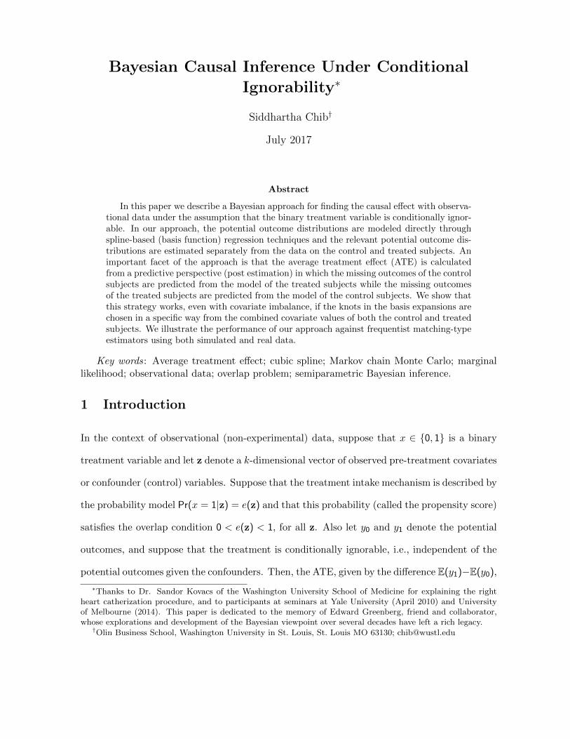
One aim of this design is to incorporate a complex dependence of the confounders on the
intake. This dependence is shown in Figure 1, which plots the propensity score for each of
the subjects in the n = 500 sample against the values of w1 and w2 for that subject. control
13
0.0 0.2 0.4 0.6 0.8 1.0
0.0
0.2
0.4
0.6
0.8
0.0
0.2
0.4
0.6
0.8
1.0
w1
w2
Pr(x=
1|w)
Figure 1: Plot of the true propensity score with simulated data (n = 500) at the generatedvalues of the confounders. The control observations are marked in circles and the treatedobservations with pluses.
subjects are indicated by circles and treated subjects by pluses. This 3-D scatterplot shows
an arch-like structure of the propensity scores. Small and large values of w1 have small values
of the propensity score and values of w1 in the mid-range of the (0, 1) interval generate larger
values of the propensity scores. As a result, there are fewer treated observations at each end
of the w1 interval.
A second aim of this design is to produce a non-trivial overlap problem. Again focusing
on the n = 500 sample, this problem can be seen from the contour plots of the (w1, w2)
distribution by intake group that are given in Figure 2. The left plot in the figure, which
has the distribution of (w1, w2)|x = 0, shows that the regions of high density (indicated by
the higher numbers on the contour lines) are separated from one another. The distribution of
(w1, w2)|x = 1 in the right side of the plot is quite different from the first distribution, with
clear regions of limited overlap.
14

0.0 0.2 0.4 0.6 0.8 1.0
0.0
0.2
0.4
0.6
0.8
1.0
x = 0 group
w1
w2
200
400
400
600
600
800
800
800
800100
0
1000
1000
1000
1200
0.0 0.2 0.4 0.6 0.8 1.0
0.0
0.2
0.4
0.6
0.8
1.0
x = 1 group
w1
w2
100
200300
400
500
500
Figure 2: Contour plot of the distribution of (w1, w2) by intake group in the simulated data(n = 500); this shows the severe overlap problem.
4.2 Model fitting
The prior distribution in (B.4) and (B.5) requires specifying the prior on two initial values for
each of the g0 and g1 functions, the priors on the variances, and the priors on the smoothness
parameters λv, λ0 and λ1. We set these priors to be same across the potential outcome models
and across models with different degrees of freedom by assuming that all regression coefficients
are centered at zero, that both variances have a gamma prior distribution with mean 1 and
standard deviation 5, and that all of the λs have means of 1 and standard deviations of 10.
Our results are based on 10,000 MCMC draws following a burn-in of 1,000 MCMC cycles.
Although we do not report the results on the mixing of the MCMC chains, the inefficiency
factors for each of the parameters in each model are mostly less than 2 or 3, indicating that
the sampling procedures are highly efficient. We assume, incorrectly, 5 degrees of freedom for
the Student-t distributions of ε0 and ε1.
We undertake a small model search as part of our fitting of the outcome models by con-
sidering models that have different number of knots in the spline formulation and 5 degrees of
freedom in the Student-t distributions. Examination of the marginal likelihoods, computed by
the method of Chib (1995) and shown in Table 1, reveals that 6 knots are sufficient for g11, and
15

that 15 knots are necessary for g12. More knots are needed in the latter equation to capture
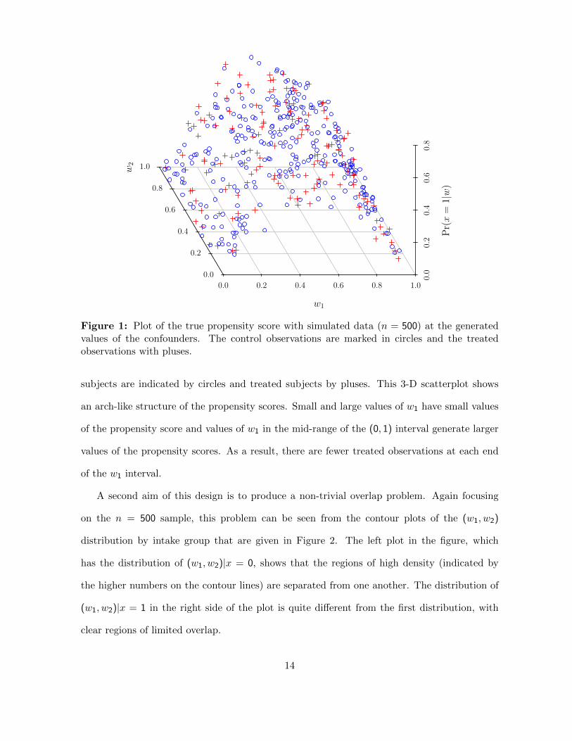
the sharp rise and fall that occurs for values of w2 between 0.4 and 0.6. In Figure 3 we show
Knots Sample Size
w1 w2 500 1,000 2,000 4,000
Controls5 5 -563.139 -1118.375 -2181.854 -4319.2716 6 -562.851 -1115.194 -2181.844 -4317.5865 10 -569.577 -1118.786 -2189.281 -4319.2836 10 -570.442 -1119.891 -2192.645 -4322.671
10 10 -572.468 -1121.318 -2199.103 -4330.002Treated
6 6 -390.496 -791.885 -1487.727 -3058.2205 10 -375.601 -753.338 -1382.359 -2821.0526 15 -366.579 -672.804 -1270.652 -2460.075
10 10 -385.074 -763.282 -1395.639 -2838.97115 15 -377.211 -687.960 -1288.669 -2489.89818 18 -378.880 -698.198 -1304.038 -2539.988
Table 1: Marginal likelihoods for the nonlinear equations, various knot combinations, simu-lated data. Knots in boldface yield greatest values of marginal likelihood.
the true functions and estimated functions for a sample of size 500.
4.3 Posterior distribution of ATE
Estimates of ATE by frequentist matching are obtained from the R package Matching. We
report results for propensity score matching based on propensity scores from a logit link and
linear covariate effects. The results are reported in Table 2.
As a simple criterion for accuracy, we determine whether the estimate ± two standard
deviations includes the true value. According to this criterion, three of the four intervals based
on propensity score matching cover the true value, and all four of the intervals based on our
Bayesian method cover the true value. Note also that the Bayesian approach yields smaller
standard deviations for all sample sizes.
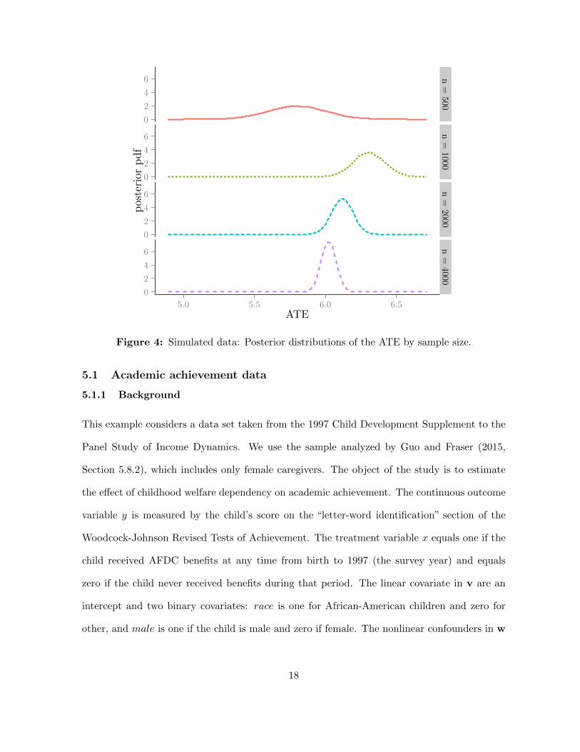
Finally, even though the data come from a complicated design, Figure 4 shows that the pos-
terior distribution of the ATE centers quickly on the true value and becomes more concentrated
as the sample size increases.
16
-0.5
0.0
0.5
1.0
1.5
0.00 0.25 0.50 0.75 1.00wc1
g c1
-5
0
5
0.00 0.25 0.50 0.75 1.00wt1
g t1
-1.5
-1.0
-0.5
0.0
0.5
1.0
0.00 0.25 0.50 0.75 1.00wc2
g c2
-4
0
4
8
0.00 0.25 0.50 0.75 1.00wt2
g t2
Figure 3: True (dotted lines) and estimated functions (solid lines) for simulated data andsample size 500.
Sample size500 1000 2000 4000
True value 6.072 6.145 6.031 6.037
Propensity Score Matching 5.726 5.732 5.728 5.544(0.332) (0.242) (0.168) (0.116)
Bayesian ATE 5.799 6.308 6.119 6.023(0.206) (0.111) (0.075) (0.053)
Table 2: True and estimated values of ATE (standard deviations in parentheses) by frequentistpropensity score matching and by the Bayes approach in the text.
5 Real data examples
This section contains the application of our method to two real data sets. The first considers
the effect on academic achievement of receiving AFDC payments, and the second examines the
effectiveness of a medical procedure on 30-day survival rates.
17
0
2
4
6
0
2
4
6
0
2
4
6
0
2
4
6
n=
500n=
1000n=
2000n=
4000
5.0 5.5 6.0 6.5ATE
posteriorpdf
Figure 4: Simulated data: Posterior distributions of the ATE by sample size.
5.1 Academic achievement data
5.1.1 Background
This example considers a data set taken from the 1997 Child Development Supplement to the
Panel Study of Income Dynamics. We use the sample analyzed by Guo and Fraser (2015,
Section 5.8.2), which includes only female caregivers. The object of the study is to estimate
the effect of childhood welfare dependency on academic achievement. The continuous outcome
variable y is measured by the child’s score on the “letter-word identification” section of the
Woodcock-Johnson Revised Tests of Achievement. The treatment variable x equals one if the
child received AFDC benefits at any time from birth to 1997 (the survey year) and equals
zero if the child never received benefits during that period. The linear covariate in v are an
intercept and two binary covariates: race is one for African-American children and zero for
other, and male is one if the child is male and zero if female. The nonlinear confounders in w
18

are mratio97, the ratio of family income to the poverty line in in 1997; pcged97, the caregiver’s
years of schooling; pcg adc, the number of years in which the caregiver received AFDC in her
childhood; and age97, the child’s age in 1997. The sample size n is 1,003, composed of n0 = 729
controls and n1 = 274 treated subjects. The ATE is expected to be negative, reflecting the
hypothesis that welfare dependency has an adverse effect on academic achievement.
Guo and Fraser (2015) examine these data with propensity score methods. They apply
a large number of matching methods and carefully show how alternative methods affect the
results. In our empirical study, we compare our Bayesian results with the matching algorithm
included in the R package Matching.
Our outcome models are specified through Student-t links with 5 degrees of freedom. The
effects of the continuous confounders are modeled by cubic splines with six knots for each
confounder. This number was determined by examination of the marginal likelihoods for 5, 6,
and 7 knots for the controls and 5 or 6 knots for the treated; we did not try 7 knots for the
treated, because of the relatively small number of observations in that group. Since the scores
are standardized with a mean of 100 and a standard deviation of 15, we set the prior expected
value of the intercept to 100, the prior expected value of the dispersion parameter σ20 to 200,
and the prior variance of σ20 to 50. Two observations were dropped from the sample because
their values for mratio96 were far larger than the other values of this variable.
5.1.2 Function estimates
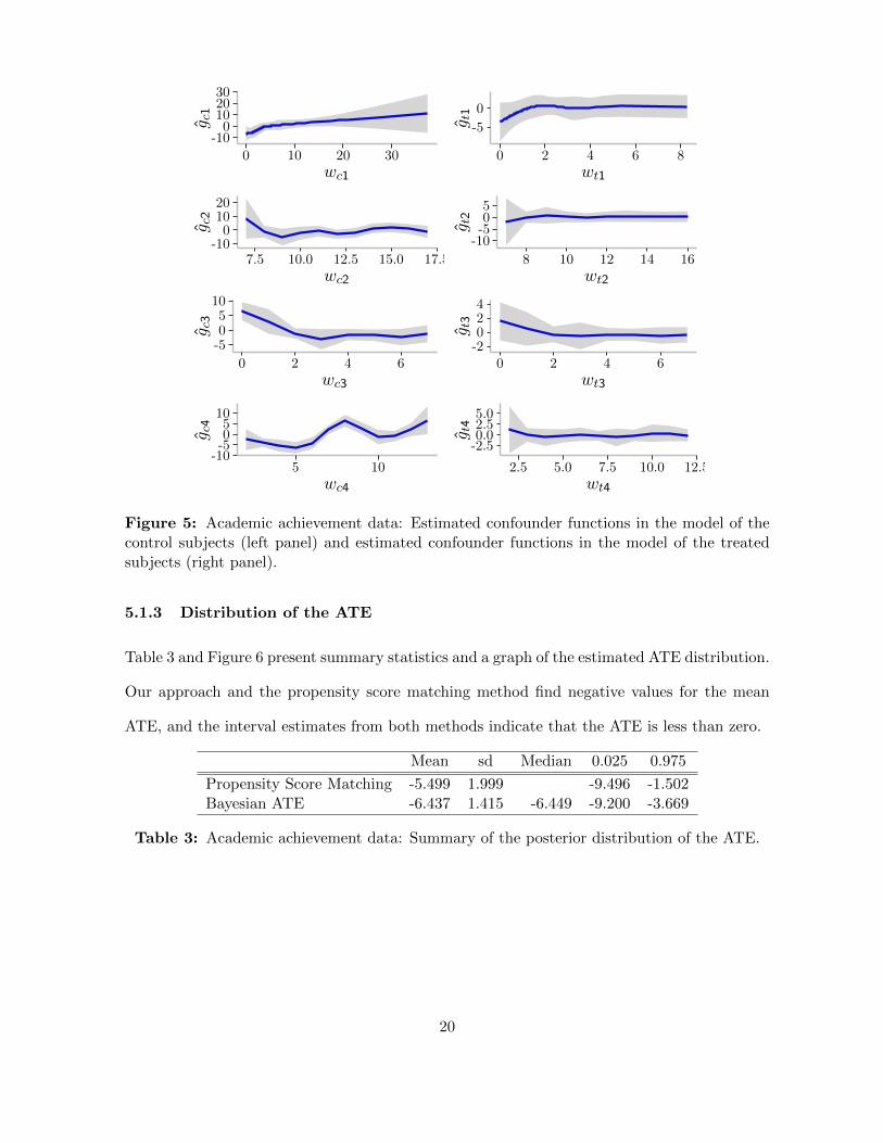
Function estimates for the four continuous variables are graphed in Figure 5. The sample of
observations on controls displays considerably more curvature than that of the treated, but, as
noted above, the Bayes factor criterion favors 6 knots for both sets of observations. We conclude
from this result that it is desirable to allow for nonlinearities in the outcome functions.
19
-100
102030
0 10 20 30wc1
g c1
-5
0
0 2 4 6 8wt1
g t1
-100
1020
7.5 10.0 12.5 15.0 17.5wc2
g c2
-10-505
8 10 12 14 16wt2
g t2
-505
10
0 2 4 6wc3
g c3
-2024
0 2 4 6wt3
g t3
-10-505
10
5 10wc4
g c4
-2.50.02.55.0
2.5 5.0 7.5 10.0 12.5wt4
g t4
Figure 5: Academic achievement data: Estimated confounder functions in the model of thecontrol subjects (left panel) and estimated confounder functions in the model of the treatedsubjects (right panel).
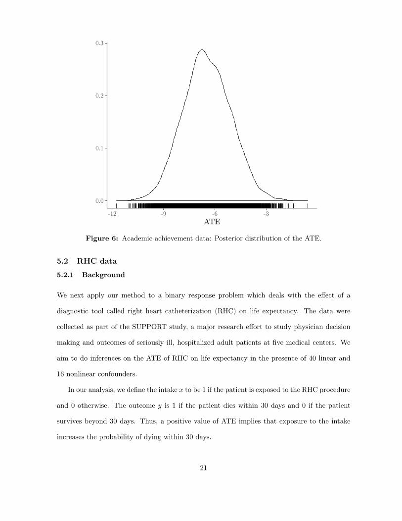
5.1.3 Distribution of the ATE
Table 3 and Figure 6 present summary statistics and a graph of the estimated ATE distribution.
Our approach and the propensity score matching method find negative values for the mean
ATE, and the interval estimates from both methods indicate that the ATE is less than zero.
Mean sd Median 0.025 0.975
Propensity Score Matching -5.499 1.999 -9.496 -1.502Bayesian ATE -6.437 1.415 -6.449 -9.200 -3.669
Table 3: Academic achievement data: Summary of the posterior distribution of the ATE.
20
0.0
0.1
0.2
0.3
-12 -9 -6 -3
ATE
Figure 6: Academic achievement data: Posterior distribution of the ATE.
5.2 RHC data
5.2.1 Background
We next apply our method to a binary response problem which deals with the effect of a
diagnostic tool called right heart catheterization (RHC) on life expectancy. The data were
collected as part of the SUPPORT study, a major research effort to study physician decision
making and outcomes of seriously ill, hospitalized adult patients at five medical centers. We
aim to do inferences on the ATE of RHC on life expectancy in the presence of 40 linear and
16 nonlinear confounders.
In our analysis, we define the intake x to be 1 if the patient is exposed to the RHC procedure
and 0 otherwise. The outcome y is 1 if the patient dies within 30 days and 0 if the patient
survives beyond 30 days. Thus, a positive value of ATE implies that exposure to the intake
increases the probability of dying within 30 days.
21

For both the controls and treated, the confounders in v consist of 40 categorical variables
that represent primary and secondary diseases, comorbidities, whether the patient has cancer
and whether it is metastatic, sex, race, income groups, insurance status, admission diagnosis,
and whether the patient chose to be resuscitated. There are 16 continuous confounders that
constitute w and these measure a variety of physical measurements and other information about
the patient taken at the time of admission into the hospital. The effects of each confounder
in w is modeled by a cubic spline. After dropping some observations because of missing and
extreme observations, our final sample contains 3,515 control and 2,163 treated subjects.
The probability of the binary outcome for both the control and treated subjects is modeled
by a Student-t link with 5 degrees of freedom. In addition, five knots are used in the cubic
spline basis expansions. This was determined by estimating models with different number
of knots and comparing the marginal likelihoods (computed by the method of Chib (1995)).
We found that the marginal likelihood dropped of considerably when more than 5 knots were
used. Thus, in each final model, there are 127 regression and basis function parameters, and
17 unknown λ smoothness parameters.
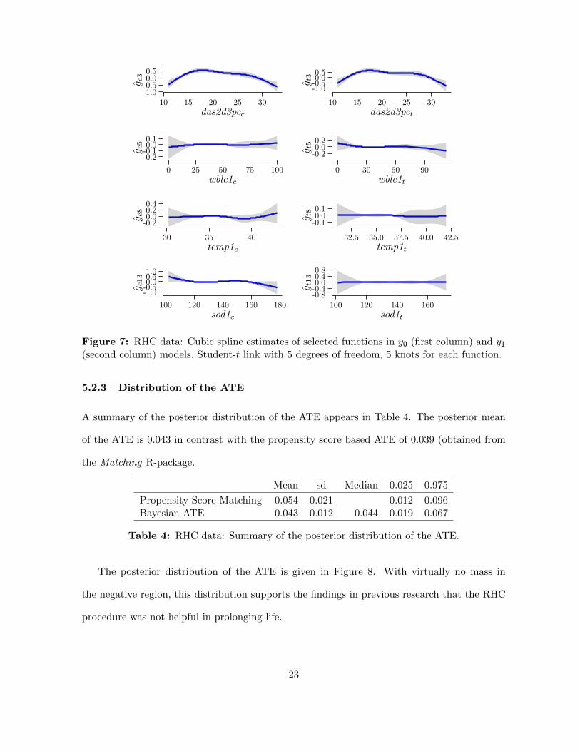
5.2.2 Function estimates
Posterior estimates of selected functions in y0 and y1 are displayed in Figure 7. The figure shows
considerable nonlinearities in the effect of the continuous variables in the outcome functions;
the effect of das2d3pc is an example. Differences in the effects of the covariates on the outcome
functions suggest that estimating the treatment effect by a simple shift in the function is not
appropriate; for example, at low values of wblc1, the probability of death increases for the
controls, but decreases for the treated, and the level of sod1 has no effect on the treated but
a highly nonlinear effect on the controls. As other examples, note that temp1 and sod1 have
nonlinear effects on the controls but no effect on the treated.
22
-1.0-0.50.00.5
10 15 20 25 30das2d3pcc
g c3
-1.0-0.50.00.5
10 15 20 25 30das2d3pct
g t3
-0.2-0.10.00.1
0 25 50 75 100wblc1c
g c5
-0.20.00.2
0 30 60 90wblc1t
g t5
-0.20.00.20.4
30 35 40temp1c
g c8
-0.10.00.1
32.5 35.0 37.5 40.0 42.5temp1t
g t8
-1.0-0.50.00.51.0
100 120 140 160 180sod1c
g c13
-0.8-0.40.00.40.8
100 120 140 160sod1t
g t13
Figure 7: RHC data: Cubic spline estimates of selected functions in y0 (first column) and y1(second column) models, Student-t link with 5 degrees of freedom, 5 knots for each function.
5.2.3 Distribution of the ATE
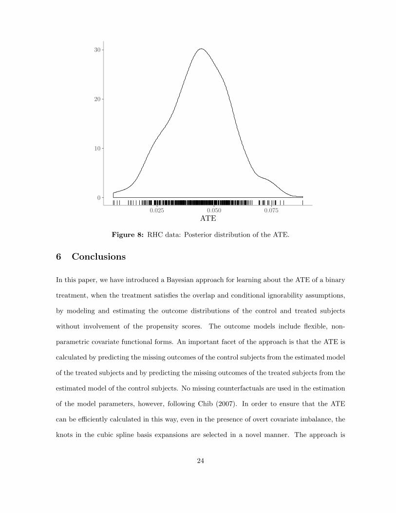
A summary of the posterior distribution of the ATE appears in Table 4. The posterior mean
of the ATE is 0.043 in contrast with the propensity score based ATE of 0.039 (obtained from
the Matching R-package.
Mean sd Median 0.025 0.975
Propensity Score Matching 0.054 0.021 0.012 0.096Bayesian ATE 0.043 0.012 0.044 0.019 0.067
Table 4: RHC data: Summary of the posterior distribution of the ATE.
The posterior distribution of the ATE is given in Figure 8. With virtually no mass in
the negative region, this distribution supports the findings in previous research that the RHC
procedure was not helpful in prolonging life.
23
0
10
20
30
0.025 0.050 0.075
ATE
Figure 8: RHC data: Posterior distribution of the ATE.
6 Conclusions
In this paper, we have introduced a Bayesian approach for learning about the ATE of a binary
treatment, when the treatment satisfies the overlap and conditional ignorability assumptions,
by modeling and estimating the outcome distributions of the control and treated subjects
without involvement of the propensity scores. The outcome models include flexible, non-
parametric covariate functional forms. An important facet of the approach is that the ATE is
calculated by predicting the missing outcomes of the control subjects from the estimated model
of the treated subjects and by predicting the missing outcomes of the treated subjects from the
estimated model of the control subjects. No missing counterfactuals are used in the estimation
of the model parameters, however, following Chib (2007). In order to ensure that the ATE
can be efficiently calculated in this way, even in the presence of overt covariate imbalance, the
knots in the cubic spline basis expansions are selected in a novel manner. The approach is
24

illustrated with both continuous and binary outcome data. The model fitting shows evidence
of nonlinear confounder effects, supporting the modeling approach advanced in this paper, and
the posterior ATE results in both the simulated and real data cases show that the method has
promise for use in practice.
APPENDIX
A Construction of the cubic spline basis matrix
Consider a single function f(w) with unknown function ordinates (f(w1), . . . , f(wn)) at each
of the sample values of the covariate w = (w1, . . . , wn). In the text, we approximate these
function values by a natural cubic spline. The basis we use is described fully in Chib and
Greenberg (2010).
We now show how to calculate the basis expansionf(w1)f(w2)
...f(wn)
= Bwβw,
where Bw is a n × (m − 1) basis matrix and βw is a (m − 1) vector of cubic spline basis
parameters. We index these quantities by w because they depend on the input vector w. The
basis functions we use for our cubic spline are the functions Φs and Ψs, s = 1, . . . ,m, have
compact support and are given by
Φs(a) =
0, a < τ s−1,
−(2/h3s)(a− τ s−1)2(a− τ s − 0.5hs), τ s−1 ≤ a < τ s,
(2/h3s+1)(a− τ s+1)2(a− τ s + 0.5hs+1), τ s ≤ a < τ s+1,
0, a ≥ τ s+1,
Ψs(a) =
0, a < τ s−1,
(1/h2s)(a− τ s−1)2(a− τ s), τ s−1 ≤ a < τ s,
(1/h2s+1)(w − τ s+1)2(a− τ s), τ s ≤ a < τ s+1,
0, a ≥ τ s+1,
where hs = τ s − τ s−1 is the spacing between the (s − 1)st and sth knots. (The basis for the
first and last knots is defined differently; see Chib and Greenberg (2010).) Next, evaluate the
25

basis functions for each element of w and each knot, and arrange them in the n×m matrices
Φ and Ψ as
Φ =
Φ1(w1) · · · Φm(w1)
......
......
......
Φ1(wn) · · · Φm(wn)
, Ψ =
Ψ1(w1) · · · Ψm(w1)
......
......
......
Ψ1(wn) · · · Ψm(wn)
.
Now let ωs = hs/(hs+hs+1), µs = 1−ωs, and define the (m×m) tri-diagonal matrix A with 2 on
the principal diagonal, (ω2, ω3, . . . , ωm−1, 1) on the first sub-diagonal, and (1, µ2, µ3, . . . , µm−1)
on the first super-diagonal. Also define the (m×m) matrix C equal to 3 times a tri-diagonal ma-
trix that has (− 1h2, ω2h2−µ2h3, . . . , ωm−1
hm−1−µm−1
hm, 1hm
) on the principal diagonal, (−ω2h2,−ω3
h3, . . . ,−ωm−1
hm−1,− 1
hm)
on the first sub-diagonal, and ( 1h2, µ2h3 , . . . ,
µm−1
hm) on the first super-diagonal. Let
B† = Φ + ΨA−1C ≡ (b1, . . . ,bm) ,
where bs ∈ <n is the sth column of B†. For identification purposes, we restrict the m
coefficients of B†, β†, by requiring∑β†k = 0 and use the restriction to eliminate
β†1 = −(β†2 + · · ·+ β†m).
The cubic spline basis matrix for a given covariate is then given by
Bw = (b2 − b1, . . . ,bm − b1)
with coefficient vector βw = (β2, . . . , βm)′. A nice property of this basis is that each component
of the cubic spline parameters βw is the value of the unknown function at the corresponding
knot i.e.,
βw =
f(τ2)...
f(τm)
.This property of the spline coefficients is particularly helpful because it aids in the formulation
of the prior distribution.
B Prior distribution
Now consider the basis coefficients of a continuous confounder wr in the control and treated
models given by β0r : (m0r − 1) × 1 and β1r : (m1r − 1) × 1. A priori we suppose that each
26

follows a discrete time, second-order Ornstein–Uhlenbeck (O-U) process, where
β0r = (β0r2, β0r3, β0r4 . . . , β0rm0r) : (m0r − 1)× 1,
β1r = (β1r2, β1r3, β1r4 . . . , β1rm1r) : (m1r − 1)× 1
are the function values at the respective knots. In defining these O-U processes, we condition on
(β0r2, β0r3) and (β1r2, β1r3). Effectively, such an assumption generalizes the second-difference
penalty in Eilers and Marx (1996) to the situation of unequally spaced knots.
The next part of the construction is the prior distribution on the initial ordinates. Instead of
an improper prior as in Lang and Brezger (2004) and Brezger and Lang (2006), this distribution
is assumed to be proper, which is necessary for utilizing marginal likelihoods for comparing
models. The hierarchical prior model is completed by specifying a flexible Gamma prior on
the smoothness parameters with the aim of achieving data-driven smoothness.
Let
∆2β0ri = (β0ri − β0ri−1)− (β0ri−1 − β0ri−2), i > 2,
and define the spacings between knots by
h0ri = τ0ri − τ0ri−1.
Then, our prior assumption on β04:m0= (β0r4, β0r5, . . . , β3rm0r) conditioned on (β0r2, β0r3) is
that
∆2β0ri = −(β0ri−1 − β0ri−2)h0ri + u0ri,
u0ri|λ0r ∼ N(
0,1
λ0rh0ri
),
where (β0ri−1 − β0ri−2)h0ri introduces mean reversion and λ0r is an unknown smoothness
parameter. Under an analogous set of assumptions for β1r we have
∆2β1ri = −(β1ri−1 − β1ri−2)h1ri + u1ri,
u1ri|λ1r ∼ N(
0,1
λ1rh1ri
),
where λ1r is another unknown smoothness parameter.
Next consider the starting ordinates, (β0r2, β0r3) and (β1r2, β1r3). Let
T−10r1:2 =(B′0rB0r
)1:2
27

denote the first two rows and columns of B′0rB0r and
T1r1:2 =(B′1rB1r
)1:2
denote the first two rows and columns of B′1rB1r. Then, our prior assumption about these
quantities is that (β0r2β0r3
)∼ N2
((β0r2,0β0r3,0
),
1
λ0rT0r1:2
)and (
β1r2β1r3
)∼ N2
((β1r2,0β1r3,0
),
1
λ1rT1r1:2
).
It is worth observing that this prior is based on only four free hyper-parameters for each
covariate, β0r2,0 and β0r3,0 for the β0r-prior, and β1r2,0 and β1r3,0 for the β1r-prior, apart
from the smoothness parameters. Our experience shows that inferences are not sensitive to
the choice of these hyperparameters. A rule of thumb is to set the hyper-parameters to equal
roughly the prior means of gr2 and gr3, if such information is available. Otherwise, these values
may be set to equal zero.
Straightforward calculations show that the foregoing prior assumptions can be conveniently
rewritten as
β0r|λ0r ∼ Nm0r−1
(D−10r β0r,0,
1
λ0rD−10r T0rD−1
′
0r
)and
β1r|λ1r ∼ Nm1r−1
(D−11r β1r,0,
1
λ1rD−11r T1rD−1
′
1r
),
where D0r and D1r are tri-diagonal matrices of the form
Djr =
1 0 0 0 ... 0 0 00 1 0 0 0 ... 0 0
(1−hjr,3)√hjr,3
(hjr,3−2)√hjr,3
1√hjr,3
0 0 0 ... 0
0(1−hjr,4)√
hjr,4
(hjr,4−2)√hjr,4
1√hjr,4
0. . .
. . ....
.... . .
. . .. . .
. . .. . .
. . ....
0. . .
. . .. . .
. . .. . .
. . ....
0 0 0 0(1−hjr.mjr−1)√
hjr,mjr−1
(hjr,mjr−2)√hjr,mjr−1
1√hjr,mr−1
0
0 0 0 0 0(1−hjr,mjr
)√hjr,mjr
(hjr,mjr−2)√hjr,mjr
1√hj,mjr
.
β0r,0 = (β0r2,0, β0r3,0, 0, . . . , 0)′ : (m0r − 1)× 1,
β1r,0 = (β1r2,0, β1r3,0, 0, . . . , 0)′ : (m1r − 1)× 1,
28
T0r = blockdiag(T0r,1:2, Im0−2) : (m0r − 1)× 1,
and
T1r = blockdiag(T1r,1:2, Im1−2) : (m1r − 1)× 1.
Thus, the penalty matrices of the g0r and g1r functions are λ0rD′0rT−10r D0r and λ1rD′1rT−11r D′1r,
respectively.
The prior of these coefficients is completed by supposing that each smoothness parameter λj
is distributed as Gamma with a prior mean of 1 and prior standard deviation of 10. Following
Claeskens et al. (2009), we also suppose that the number of knots increases with the sample
size as does the size of each size λj . We thus suppose that the prior mean of λj is adjusted
upwards with n and the number of knots. Finally, the prior on the coefficients of the linear
covariates is joint normal and on the error dispersion σ2j is inverse-gamma.
References
Albert, J. H. and Chib, S. (1993), “Bayesian analysis of binary and polychotomous responsedata,” Journal of the American Statistical Association, 88, 669–679.
An, W. (2010), “Bayesian Propensity Score Estimators: Incorporating Uncertainties In Propen-sity Scores Into Causal Inference,” Sociological Methodology, Vol 40, 40, 151–189.
Brezger, A. and Lang, S. (2006), “Generalized structured additive regression based on BayesianP -splines,” Computational Statistics & Data Analysis, 50, 967–99.
Chib, S. (1995), “Marginal likelihood from the Gibbs output,” Journal of the American Statis-tical Association, 90, 1313–1321.
— (2007), “Analysis of treatment response data without the joint distribution of potentialoutcomes,” Journal of Econometrics, 140, 401–412.
Chib, S. and Greenberg, E. (2010), “Additive cubic spline regression with Dirichlet processmixture errors,” Journal of Econometrics, 156, 322–336.
Claeskens, G., Krivobokova, T., and Opsomer, J. D. (2009), “Asymptotic properties of penal-ized spline estimators,” Biometrika, 96, 529–544.
Eilers, P. H. C. and Marx, B. D. (1996), “Flexible Smoothing with B -Splines and Penalties(with discussion),” Statistical Science, 11, 89–121.
Guo, S. and Fraser, M. W. (2015), Propensity Score Analysis: Statistical Methods and Applica-tions, Advanced Quantitative Techniques in the Social Sciences, Thousand Oaks, CA: Sage,2nd ed.
29

Hill, J. L. (2011), “Bayesian Nonparametric Modeling for Causal Inference,” Journal of Com-putational and Graphical Statistics, 20, 217–240.
Hoshino, T. (2008), “A Bayesian propensity score adjustment for latent variable modeling andMCMC algorithm,” Computational Statistics & Data Analysis, 52, 1413–1429.
Kaplan, D. and Chen, J. S. (2012), “A Two-Step Bayesian Approach for Propensity ScoreAnalysis: Simulations and Case Study,” Psychometrika, 77, 581–609.
Lang, S. and Brezger, A. (2004),“Bayesian P -Splines,”Journal of Computational and GraphicalStatistics, 13, 183–212.
McCandless, L. C., Gustafson, P., and Austin, P. C. (2009), “Bayesian propensity score analysisfor observational data,” Statistics in Medicine, 28, 94–112.
Rosenbaum, P. R. and Rubin, D. B. (1983), “The central role of the propensity score inobservational studies for causal effects,” Biometrika, 70, 41–55.
Saarela, O., Belzile, L. R., and Stephens, D. A. (2016), “A Bayesian view of doubly robustcausal inference,” Biometrika, 103, 667–681.
Wang, C., Parmigiani, G., and Dominici, F. (2012), “Bayesian Effect Estimation Accountingfor Adjustment Uncertainty,” Biometrics, 68, 661–671.
Zigler, C. M., Watts, K., Yeh, R. W., Wang, Y., Coull, B. A., and Dominici, F. (2013), “ModelFeedback in Bayesian Propensity Score Estimation,” Biometrics, 69, 263–273.
30
Related Documents