Applied Probability Trust (17 December 2002) BAYESIAN, GEOMETRIC SUBSPACE TRACKING ANUJ SRIVASTAVA, * Florida State University ERIC KLASSEN, ** Florida State University Abstract We address the problem of tracking the time-varying linear subspaces (of a larger system) under a Bayesian framework. Variations in subspaces are treated as a piecewise-geodesic process on a complex Grassmann manifold and a Markov prior is imposed on it. This prior model, together with an observation model, gives rise to a hidden Markov model on a Grassmann manifold, and admits Bayesian inferences. A sequential Monte Carlo method is used for sampling from the time-varying posterior and the samples are utilized to estimate the underlying process. Simulation results are presented for principal subspace tracking in array signal processing. Keywords: Subspace tracking, Grassmann manifold, Bayesian tracking, non- Euclidean filtering, sequential Monte Carlo. AMS 2000 Subject Classification: Primary 93E11 Secondary 94A11;65C35 1. Introduction Many applications in signal processing, image analysis, computational biology, and environmental statistics involve inferences on large-dimensional, time-varying systems. Since most sophisticated statistical procedures are limited to smaller spaces, a common strategy is to project the observations from larger spaces to low-dimensional subspaces, and then apply the statistical procedures. In view of their simplicity and computational efficiency, the linear projections are commonly used for this purpose. Examples include principal component analysis, independent components, and Fisher’s discriminants. Different linear projections result from different optimality criteria. For example, * Postal address: Department of Statistics, Florida State University, Tallahassee, FL 32306 ** Postal address: Department of Mathematics, Florida State University, Tallahassee, FL 32306 1

Welcome message from author
This document is posted to help you gain knowledge. Please leave a comment to let me know what you think about it! Share it to your friends and learn new things together.
Transcript
Applied Probability Trust (17 December 2002)
BAYESIAN, GEOMETRIC SUBSPACE TRACKING
ANUJ SRIVASTAVA,∗ Florida State University
ERIC KLASSEN,∗∗ Florida State University
Abstract
We address the problem of tracking the time-varying linear subspaces (of
a larger system) under a Bayesian framework. Variations in subspaces are
treated as a piecewise-geodesic process on a complex Grassmann manifold and
a Markov prior is imposed on it. This prior model, together with an observation
model, gives rise to a hidden Markov model on a Grassmann manifold, and
admits Bayesian inferences. A sequential Monte Carlo method is used for
sampling from the time-varying posterior and the samples are utilized to
estimate the underlying process. Simulation results are presented for principal
subspace tracking in array signal processing.
Keywords: Subspace tracking, Grassmann manifold, Bayesian tracking, non-
Euclidean filtering, sequential Monte Carlo.
AMS 2000 Subject Classification: Primary 93E11
Secondary 94A11;65C35
1. Introduction
Many applications in signal processing, image analysis, computational biology, and
environmental statistics involve inferences on large-dimensional, time-varying systems.
Since most sophisticated statistical procedures are limited to smaller spaces, a common
strategy is to project the observations from larger spaces to low-dimensional subspaces,
and then apply the statistical procedures. In view of their simplicity and computational
efficiency, the linear projections are commonly used for this purpose. Examples include
principal component analysis, independent components, and Fisher’s discriminants.
Different linear projections result from different optimality criteria. For example,
∗ Postal address: Department of Statistics, Florida State University, Tallahassee, FL 32306∗∗ Postal address: Department of Mathematics, Florida State University, Tallahassee, FL 32306
1

2 Srivastava and Klassen
maximizing the variance of the projected variables results in principal components
[8], and minimizing the mutual information between them leads to independent com-
ponents [2]. Since the original larger system is time-varying, one has to find an optimal
projection for each time or, in other words, find a time sequence of optimal projections.
Equivalently, one can estimate a time sequence of optimal subspaces using observations
from the original system. This task of estimating a sequence of subspaces of a time-
varying system is called subspace tracking.
To illustrate the problem of tracking principal subspaces, consider a time-varying
system taking values in Cn, for a large n. We are interested in tracking m-dimensional
principal subspaces of Cn (m ≤ n) using the observed data. Let Yt = [yt,1 yt,2 . . . yt,p],
yt,i ∈ Cn be the set of p (p ≥ m) observations collected in a small interval around time
t. The space spanned by the m-dominant eigenvectors of the sample covariance matrix
Kt ∈ Cn×n estimates the principal subspace at time t. Here
Kt =1
p− 1
p∑i=1
(yt,i − yt) (yt,i − yt)†, yt =1p
p∑i=1
yt,i , (1)
where † denotes conjugate transpose. Shown in the left panel of Figure 1 is a pictorial
illustration of subspace tracking for n = 2 and m = 1. This panel shows observations for
times t = 1 in dots and t = 2 in ’+’, and the corresponding estimated one-dimensional
subspaces. The goal is to track the rotation of these subspaces as new observations are
made at regular intervals.
Q
P
U
I
PI
U(n)H
UH
X
t=0
t=1
α
β
Q
PPI
P2
P1
αα∼
t=0
t=1
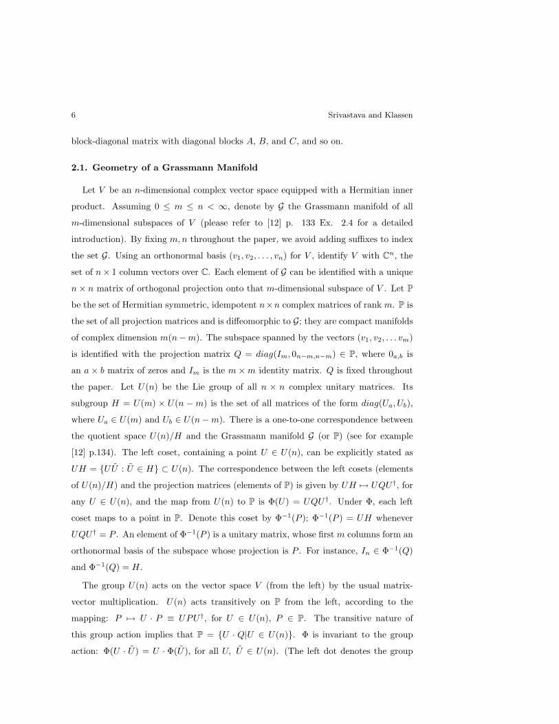
Figure 1: Left panel: estimation of subspaces at two separate times. Middle panel: Finding
a geodesic path connecting Q to P on P by lifting it to a specific geodesic path in U(n). Last
panel: Finding a geodesic path between P1 and P2 by rotating them to Q and some P ∈ P.
Geometric Subspace Tracking 3
As an application, we will consider the following problem in array signal processing.
An array of electromagnetic sensors, arranged linearly on the ground at uniform
spacing, records incident signals (at a known wavelength) from multiple, ground-based,
mobile signal transmitters. The goal is to detect and track angular locations of the
signal transmitters using data recorded by the array. An important intermediate goal
is to track the signal subspace, the subspace spanned by the transmitters, using data
collected in noisy environments (see [17] for details). Given a signal subspace, there are
efficient algorithms for computing the transmitters’ locations. Assuming that the signal
energies exceed the noise energy, and assuming m signal transmitters for n sensors in
the array (m < n), m-dimensional principal subspace of the data estimates the signal
subspace, and we are interested in tracking it. Pre-processing of signals makes the
sensor recording at each time a complex number; the array output at each time is an
element of Cn. A statistical model for array data is given later in Section 3.2.
Several approaches have been presented in the literature for estimating and tracking
subspaces, with applications to signal processing (see [20, 3] and the references therein).
While most approaches rely on relating the observations across time (for example using
windowing methods) and then estimating the principal subspaces, our focus is on inves-
tigating geometric representations and resulting procedures that can handle tracking
of arbitrary subspaces. Our ideas are also applicable to tracking on quotient spaces of
general (finite-dimensional) Lie groups. Through the introduction of a prior model on
the evolution of subspaces, we will treat subspace tracking as a problem in Bayesian
inference. The first issue is: On what space should the subspace tracking problem be
posed? A natural way to represent subspaces is as elements of a Grassmann manifold,
the set of all (fixed-dimensional) subspaces of a larger vector space ([5, 18]). This
subspace tracking on Grassmann manifold extends the Bayesian framework introduced
in [18] for estimating time-invariant subspaces. A distinct advantage of the Bayesian
approach is its ability to estimate the trajectories of subspaces as a whole rather than
estimating individual subspaces. This tackles an important issue in subspace tracking
that, at any given time, there may not be enough observations for estimating each
of the subspaces individually to a required precision, i.e. p (in the definition of Kt)
may be small. Often the observations are too noisy to provide a reliable estimate at
each observation time. An obvious choice, in such problems relating to time-series
4 Srivastava and Klassen
estimation, is to utilize a temporal structure or a prior model to treat tracking as
Bayesian estimation of an underlying stochastic process. We will follow the approach
of [16] where, in the context of tracking airplanes using remote sensing, the Newtonian
equations of motion provide a prior model for Bayesian tracking. Such a prior, in
effect, imposes a smoothness constraint on the estimated trajectories. This effect has
also been achieved directly in [9] by fitting smooth curves for a given number of points
on a particular Grassmann manifold (CP1).
How does one model a stochastic process on a Grassmann manifold? We will model
the process as a piecewise geodesic curve, and will impose a Markov prior on the
random variables associated with the individual pieces. In particular, geodesic curves
help define the notion of velocities, and a stochastic difference equation involving the
velocities provides the desired model. Our motivation for such a model is that a
stochastic process with smooth sample paths can be easily modeled by a linear equation
on its velocities. An observation model provides a likelihood function for completing
the Bayesian formulation.
In order to define geodesics on a Grassmann manifold, one has to study its intrinsic
geometry. Let G be the Grassmann manifold of all m-dimensional complex subspaces
of Cn. Any element of this manifold, i.e. any m-dimensional subspace of C
n, can
either be represented by its projection operator (uniquely) or by an orthonormal basis
(non-uniquely). Choosing the projection matrices to represent subspaces, we will
construct geodesics between two arbitrary projection matrices. Since a Grassmannian
is a quotient space of a larger unitary group, modulo a subgroup, this geodesic is made
explicit by lifting it to a particular geodesic in the unitary group. Furthermore, the
tangents to the lifted geodesic curve in the unitary group help define the velocities
associated with a curve on Grassmann manifold. A similar construction of geodesics
on the well-studied shape spaces is given in [13].
The next task is to develop algorithms for tracking. In view of the inherent non-
linearities present in the model, and the problem formulation on curved manifolds,
the classical Kalman-filtering framework does not apply. For Euclidean systems, a
number of solutions including the extended Kalman filters, interacting multiple models,
multiple hypothesis tests, and their combinations, have been suggested. However, there
is little discussion in the literature on non-Euclidean tracking. We take a Monte Carlo
Geometric Subspace Tracking 5
approach to subspace tracking. This procedure is based on the particle filtering or the
sequential Monte Carlo method. It involves sampling from the prior and resampling
them according to their likelihoods in order to generate samples from the posterior, at
each observation time. These samples are then averaged to estimate the underlying
subspaces. This technique is popular for tracking in Euclidean spaces [6, 15], with a
related idea presented in [16].
The main contributions of this paper are: (i) Posing subspace tracking as a problem
in estimating a stochastic process on a complex Grassmann manifold, (ii) imposing a
Markovian prior on the process using geodesic paths and treating subspace tracking as
a problem in Bayesian inference, and (iii) applying a sequential Monte Carlo algorithm
to sample from the time-varying posterior. In addition to tracking subspaces, this
sampling also allows for the estimation of expected errors and other posterior moments
for performance diagnostics, as described in [19].
The paper is organized as follows. Section 2 utilizes the intrinsic geometry of a
Grassmann manifold to define geodesics, and suggests a prior model on the subspace
process. Section 3 presents a Bayesian formulation of subspace tracking and Section 4
describes a sequential Monte Carlo method for generating inferences. Some simulation
results, illustrating the algorithm for a particular problem in array signal subspace
tracking, are presented in Section 5.
2. Representation of Subspace Trajectories
Subspace estimation and tracking are important to many applications. Even though
these inference problems are naturally posed on Grassmann manifolds, the use of
geometric techniques has only been recent [1, 5, 18] . In this section, we study the
intrinsic geometry of a Grassmann manifold and specify geodesics between arbitrary
points on this manifold.
For any two matrices A and B, we will use diag(A,B) to denote a matrix
A 0A
0B B
,
where 0A, 0B are matrices of zeros with appropriate sizes. For example, 0A has same
number of columns as B and same number of rows as A. Similarly, define cdiag(A,B)
to be the matrix
0A A
B 0B
. This notation generalizes, e.g. diag(A,B,C) implies a
6 Srivastava and Klassen
block-diagonal matrix with diagonal blocks A, B, and C, and so on.
2.1. Geometry of a Grassmann Manifold
Let V be an n-dimensional complex vector space equipped with a Hermitian inner
product. Assuming 0 ≤ m ≤ n < ∞, denote by G the Grassmann manifold of all
m-dimensional subspaces of V (please refer to [12] p. 133 Ex. 2.4 for a detailed
introduction). By fixing m,n throughout the paper, we avoid adding suffixes to index
the set G. Using an orthonormal basis (v1, v2, . . . , vn) for V , identify V with Cn, the
set of n× 1 column vectors over C. Each element of G can be identified with a unique
n× n matrix of orthogonal projection onto that m-dimensional subspace of V . Let P
be the set of Hermitian symmetric, idempotent n×n complex matrices of rank m. P is
the set of all projection matrices and is diffeomorphic to G; they are compact manifolds
of complex dimension m(n−m). The subspace spanned by the vectors (v1, v2, . . . vm)
is identified with the projection matrix Q = diag(Im, 0n−m,n−m) ∈ P, where 0a,b is
an a × b matrix of zeros and Im is the m ×m identity matrix. Q is fixed throughout
the paper. Let U(n) be the Lie group of all n × n complex unitary matrices. Its
subgroup H = U(m) × U(n −m) is the set of all matrices of the form diag(Ua, Ub),
where Ua ∈ U(m) and Ub ∈ U(n−m). There is a one-to-one correspondence between
the quotient space U(n)/H and the Grassmann manifold G (or P) (see for example
[12] p.134). The left coset, containing a point U ∈ U(n), can be explicitly stated as
UH = UU : U ∈ H ⊂ U(n). The correspondence between the left cosets (elements
of U(n)/H) and the projection matrices (elements of P) is given by UH 7→ UQU†, for
any U ∈ U(n), and the map from U(n) to P is Φ(U) = UQU†. Under Φ, each left
coset maps to a point in P. Denote this coset by Φ−1(P ); Φ−1(P ) = UH whenever
UQU† = P . An element of Φ−1(P ) is a unitary matrix, whose first m columns form an
orthonormal basis of the subspace whose projection is P . For instance, In ∈ Φ−1(Q)
and Φ−1(Q) = H.
The group U(n) acts on the vector space V (from the left) by the usual matrix-
vector multiplication. U(n) acts transitively on P from the left, according to the
mapping: P 7→ U · P ≡ UPU†, for U ∈ U(n), P ∈ P. The transitive nature of
this group action implies that P = U · Q|U ∈ U(n). Φ is invariant to the group
action: Φ(U · U) = U · Φ(U), for all U, U ∈ U(n). (The left dot denotes the group
Geometric Subspace Tracking 7
action on U(n) while the right dot denotes the group action on P.) The tangent
space of U(n) at identity is u(n), the space of n × n, Hermitian skew-symmetric
matrices (see for example [21] p. 107). Let H be a subset of u(n) defined as:
H =diag(Ya, Yb)| Ya ∈ C
m×m, Yb ∈ C(n−m)×(n−m) are Hermitian skew-symmetric
.
Let M be the orthogonal complement of H in u(n):
M =
cdiag(A,−A†) ∈ Cn×n : A ∈ C
m(n−m)⊂ u(n) . (2)
As a compact Lie group, U(n) is equipped with a unique bi-invariant Riemannian
metric, which is inherited by P. On u(n), this metric is just the inner product
〈Y1 , Y2〉 = trace(Y1Y†2 ). Since 〈UY1 , UY2〉 = 〈Y1 , Y2〉, for any U ∈ U(n), this metric
is invariant to the left translation generated by the group action.
2.2. Geodesics on Grassmann Manifold
We will represent a stochastic process on P as a piecewise-geodesic curve with
random velocities at individual pieces. Therefore, we need an explicit description of
geodesics on P. This is done in two steps: (i) first construct a geodesic between Q and
any P ∈ P, and then (ii) construct a geodesic between any two P1, P2 ∈ P. We start
with a specification of geodesics passing through the point Q.
Proposition 1. The geodesics in P passing through the point Q (at time t = 0) are
of the type α : (−ε, ε) 7→ P, α(t) = exp(tX) · Q = exp(tX)Q exp(−tX), for some
X ∈M, where the set M is specified in Eqn. 2.
Proof: This proposition is identical to the exercise 2(i) on p.226 in [7]. We sketch
a proof here. Let α be the geodesic in P connecting Q (at t = 0) with a point P
(at t = 1). Geodesics in P can be made explicit via corresponding geodesics in U(n),
since P is identified with the quotient space U(n)/H. The geodesics in U(n), passing
through a point U ∈ U(n), are known to be the one-parameter subgroups of the type
β(t) = exp(tX) · U for any X ∈ u(n). The geodesic β (in U(n)) projects down to a
geodesic α (in P) if and only if β is orthogonal to each coset that it intersects in U(n).
On the other hand, invariance of the metric (last line of Section 2.1) implies that if β
is orthogonal to one coset, then it is orthogonal to each and every coset it intersects.
In particular, if β passes through I (at t = 0), it should be orthogonal to the coset
H (i.e. β(0) ⊥ H). For β(t) = exp(tX) · I, this condition implies that X belongs to
8 Srivastava and Klassen
the orthogonal complement of H in u(n), namely M. Finally, the projection of β to
P gives α, using the invariance of Φ, α(t) = Φ(β(t)) = exp(tX)Q exp(−tX). Shown
in the middle panel of Figure 1 is an illustration of defining geodesics in P by lifting
to a geodesic in U(n) such that they are always orthogonal to cosets in U(n). In this
picture, the cosets are denoted by vertical lines.
According to Proposition 1, α is completely specified by an X ∈ M such that
exp(X)Q exp(−X) = P . Therefore, the problem of finding α becomes:
Problem 1: Given a point P ∈ P, find an X ∈M such that exp(X)Q exp(−X) = P .
Note that for this X, exp(X) in addition to being in Φ−1(P ), is nearest to I among
all elements of the set Φ−1(P ).
We start the solution by motivate the case n = 2, m = 1.
Example 1: Consider a two-dimensional vector space V . Let (v1, v2) be an ordered
orthonormal basis for V and Q = diag(1, 0) be the projection matrix of the subspace
spanned by v1. Let P denote (the projection matrix of) the one-dimensional subspace
spanned by cos(α)v1 + sin(α)v2, for some α > 0. Then, P is given by U(α)QU(α)T or cos2(α) cos(α) sin(α)
cos(α) sin(α) sin2(α)
, where U(α) =
cos(α) − sin(α)
sin(α) cos(α)
.
Eigen decomposition of Q − P is given by WΣW †, where Σ = diag(sin(α),− sin(α)),
and the columns of W are the corresponding eigenvectors. Since Q − P is Hermitian
symmetric, W can be taken to be a unitary matrix. We require that Qw1 is a positive
real multiple of Qw2, where w1, w2 are the two columns of W . This can be achieved
simply by multiplying w1 by an appropriate unit complex number (see Remark 1 later).
Returning to the task of finding X as per Problem 1, it follows that:
X = WΩW †, and exp(X) = W exp(Ω)W †, where Ω = cdiag(−α, α) . (3)
In this 2× 2 case WΩW † happens to be the same as Ω. This example suggests a role
for the eigen decomposition of Q− P in finding X.
Theorem 1. For a point P ∈ P, let B = WΣW † be the eigen decomposition of B =
Q− P such that W is a unitary matrix. Then,
1. the eigenvalues of B (or the diagonal entries of Σ) are either 0’s or occur in
pairs of the form (λj ,−λj), where 0 < λj ≤ 1. Qwj and Qwj′ can be chosen
Geometric Subspace Tracking 9
to be positive real multiples of each other, where wj, wj′ are the columns of W
corresponding to the eigenvalues λj and −λj, respectively, for all j’s. This can
be accomplished using the procedure in Remark 2.
2. Let Ω be a n×n matrix derived from Σ in the following way: replace all the 2×2
blocks diag(λj ,−λj) by cdiag(− sin−1(λj), sin−1(λj)), with the remaining entries
staying zeros. Then, set X to be WΩW † ∈M.
3. Set exp(X) = W ΩW † ∈ U(n), where Ω is formed from Σ by replacing: (i)
the zeros in the diagonal by ones, and (ii) the 2 × 2 blocks diag(λj ,−λj) by
√1− λ2
j −λj
λj
√1− λ2
j
.
4. A geodesic in P from Q to P is then given by exp(tX)Q exp(−tX) for 0 ≤ t ≤ 1.
Proof: Please refer to the Appendix.
Remark 1: We require that Qwj be a positive multiple of Qwj′ for all js. If λj ’s
are all distinct, this can be achieved by multiplying wj by the unit complex number:
c = c/|c|, where c = wj′ (1)wj(1)
, and wk(1) is the first element of the vector wk. If several
λj ’s are the same, with the corresponding columns w1, . . . , ws, we will alter the
columns w1′ , . . . , ws′ as follows. For each i = 1 . . . , s, there is a unique unit vector
yi ∈ spanw1′ , . . . , ws′ with the property that Qyi is a positive real multiple of Qwi.
For each such i = 1, . . . , s, replace wi′ by yi. Continue to call the resulting matrix W .
This completes the necessary modification of W .
We note that for certain points in P (analogous to diametrically opposite points
on a sphere), the matrix X, and therefore, the resulting geodesic may not be unique.
In the context of subspace tracking, these pairs occur in P × P with zero probability,
and hence are ignored. Also, note that the computational cost of calculating X is
essentially that of finding the eigen decomposition of Q− P .
The next step is to find a geodesic between two arbitrary two points P1, P2 in
P. The basic idea is to rotate these points back to Q and P (for some P ∈ P),
respectively and then apply Theorem 1. Let U ∈ Φ−1(P1) (that is, P1 = UQU†)
and define P = U †P2U . Then, using Theorem 1, we can find an X such that α(t) =
exp(tX) · Q is a geodesic from Q to P . Define a shifted geodesic α according to
10 Srivastava and Klassen
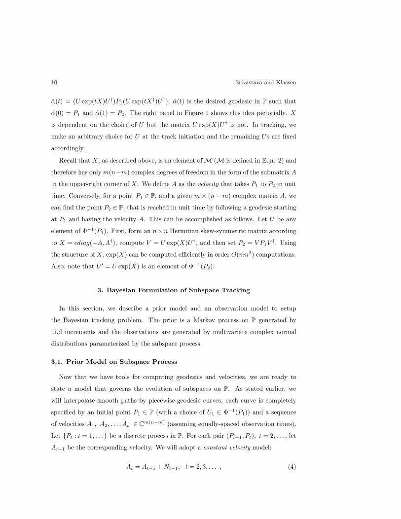
α(t) = (U exp(tX)U†)P1(U exp(tX†)U†); α(t) is the desired geodesic in P such that
α(0) = P1 and α(1) = P2. The right panel in Figure 1 shows this idea pictorially. X
is dependent on the choice of U but the matrix U exp(X)U† is not. In tracking, we
make an arbitrary choice for U at the track initiation and the remaining Us are fixed
accordingly.
Recall that X, as described above, is an element ofM (M is defined in Eqn. 2) and
therefore has only m(n−m) complex degrees of freedom in the form of the submatrix A
in the upper-right corner of X. We define A as the velocity that takes P1 to P2 in unit
time. Conversely, for a point P1 ∈ P, and a given m× (n−m) complex matrix A, we
can find the point P2 ∈ P, that is reached in unit time by following a geodesic starting
at P1 and having the velocity A. This can be accomplished as follows. Let U be any
element of Φ−1(P1). First, form an n×n Hermitian skew-symmetric matrix according
to X = cdiag(−A,A†), compute V = U exp(X)U†, and then set P2 = V P1V†. Using
the structure of X, exp(X) can be computed efficiently in order O(nm2) computations.
Also, note that U ′ = U exp(X) is an element of Φ−1(P2).
3. Bayesian Formulation of Subspace Tracking
In this section, we describe a prior model and an observation model to setup
the Bayesian tracking problem. The prior is a Markov process on P generated by
i.i.d increments and the observations are generated by multivariate complex normal
distributions parameterized by the subspace process.
3.1. Prior Model on Subspace Process
Now that we have tools for computing geodesics and velocities, we are ready to
state a model that governs the evolution of subspaces on P. As stated earlier, we
will interpolate smooth paths by piecewise-geodesic curves; each curve is completely
specified by an initial point P1 ∈ P (with a choice of U1 ∈ Φ−1(P1)) and a sequence
of velocities A1, A2, . . . , At ∈ Cm(n−m) (assuming equally-spaced observation times).
Let Pt : t = 1, . . . be a discrete process in P. For each pair (Pt−1, Pt), t = 2, . . . , let
At−1 be the corresponding velocity. We will adopt a constant velocity model:
At = At−1 + Nt−1, t = 2, 3, . . . , (4)

Geometric Subspace Tracking 11
where Nt−1 is a m × (n −m) matrix of i.i.d complex normals (real, imaginary parts
are i.i.d normal with mean zero and variance σ2p). σp is the deviation of At, away from
a given value of At−1 and can be estimated from the past trajectories.
In a Markovian time-series analysis, there is often a characterization of a time-
varying posterior density, in a convenient recursive form. This characterization involves
a hidden Markov chain, with given transition densities, and an observation sequence,
with a given observation model. To obtain Markovity, we consider the chain on the joint
space of subspaces and velocities. Define the subspace-velocity pair Jt = (Pt, At−1) ∈(P×C
m(n−m)), for each time t. Jt is a discrete-time Markov process. For the purpose
of defining velocities At’s, we will keep track of the corresponding Ut’s in Φ−1(Pt)’s.
(Note that given any two of the Pt, Pt−1, and At−1, the remaining third is completely
determined.) This setup leads to the following transition density:
f(Jt|Jt−1) = f(At−1|At−2)f(Pt|At−1, Pt−1, At−2) = f(At−1|At−2)δP ′t(Pt)
where P ′t = Vt−1Pt−1V
†t−1 and Vt−1 = Ut−1 exp(Xt−1)U
†t−1, Xt−1 = cdiag(−At−1, A
†t−1) ,
for any Ut−1 ∈ Φ−1(Pt−1). The conditional density f(At−1|At−2) follows from Eqn. 4
and δP1(P2) denotes a delta dirac function on P centered at P2. For the next time step,
set Ut = Ut−1 exp(Xt−1) ∈ Φ−1(Pt). The following algorithm specifies a procedure to
sample from this Markov model:
Algorithm 1. For some t = 2, 3, . . . , we are given the values for J(i)t−1 and points
U(i)t−1 ∈ Φ−1(P (i)
t−1). For i = 1, 2, . . . , M :
1. Generate a sample of A(i)t−1, given A
(i)t−2, according to Eqn. 4.
2. For each sample of A(i)t−1, set X
(i)t−1 = cdiag(−A
(i)t−1, (A
(i)t−1)
†), and calculate P(i)t
according to P(i)t = V
(i)t−1P
(i)t−1(V
(i)t−1)
†, for V(i)t−1 = U
(i)t−1 exp(X(i)
t−1)(U(i)t−1)
†.
3. Define the sampled subspace-velocity pair J(i)t = (P (i)
t , A(i)t−1). Set U
(i)t = U
(i)t−1 exp(X(i)
t−1).
3.2. Observation Model
In principle, this framework allows for any density function relating the hidden
Markov chain Jt to the observed data Yt. Different choices of densities will lead
to different specifications of subspaces. In the case of array signal processing and
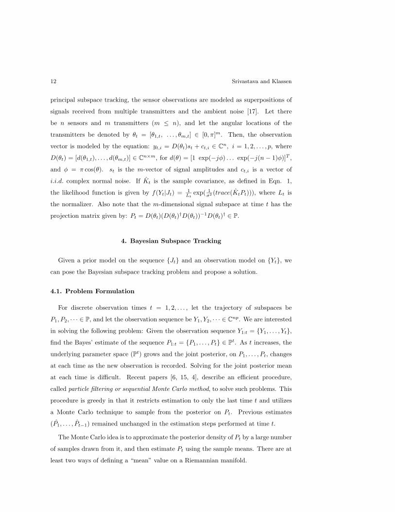
12 Srivastava and Klassen
principal subspace tracking, the sensor observations are modeled as superpositions of
signals received from multiple transmitters and the ambient noise [17]. Let there
be n sensors and m transmitters (m ≤ n), and let the angular locations of the
transmitters be denoted by θt = [θ1,t, . . . , θm,t] ∈ [0, π]m. Then, the observation
vector is modeled by the equation: yt,i = D(θt)st + ct,i ∈ Cn, i = 1, 2, . . . , p, where
D(θt) = [d(θ1,t), . . . , d(θm,t)] ∈ Cn×m, for d(θ) = [1 exp(−jφ) . . . exp(−j(n − 1)φ)]T ,
and φ = π cos(θ). st is the m-vector of signal amplitudes and ct,i is a vector of
i.i.d. complex normal noise. If Kt is the sample covariance, as defined in Eqn. 1,
the likelihood function is given by f(Yt|Jt) = 1Lt
exp( 1σ2 (trace(KtPt))), where Lt is
the normalizer. Also note that the m-dimensional signal subspace at time t has the
projection matrix given by: Pt = D(θt)(D(θt)†D(θt))−1D(θt)† ∈ P.
4. Bayesian Subspace Tracking
Given a prior model on the sequence Jt and an observation model on Yt, we
can pose the Bayesian subspace tracking problem and propose a solution.
4.1. Problem Formulation
For discrete observation times t = 1, 2, . . . , let the trajectory of subspaces be
P1, P2, · · · ∈ P, and let the observation sequence be Y1, Y2, · · · ∈ Cnp. We are interested
in solving the following problem: Given the observation sequence Y1:t = Y1, . . . , Yt,find the Bayes’ estimate of the sequence P1:t = P1, . . . , Pt ∈ P
t. As t increases, the
underlying parameter space (Pt) grows and the joint posterior, on P1, . . . , Pt, changes
at each time as the new observation is recorded. Solving for the joint posterior mean
at each time is difficult. Recent papers [6, 15, 4], describe an efficient procedure,
called particle filtering or sequential Monte Carlo method, to solve such problems. This
procedure is greedy in that it restricts estimation to only the last time t and utilizes
a Monte Carlo technique to sample from the posterior on Pt. Previous estimates
(P1, . . . , Pt−1) remained unchanged in the estimation steps performed at time t.
The Monte Carlo idea is to approximate the posterior density of Pt by a large number
of samples drawn from it, and then estimate Pt using the sample means. There are at
least two ways of defining a “mean” value on a Riemannian manifold.
Geometric Subspace Tracking 13
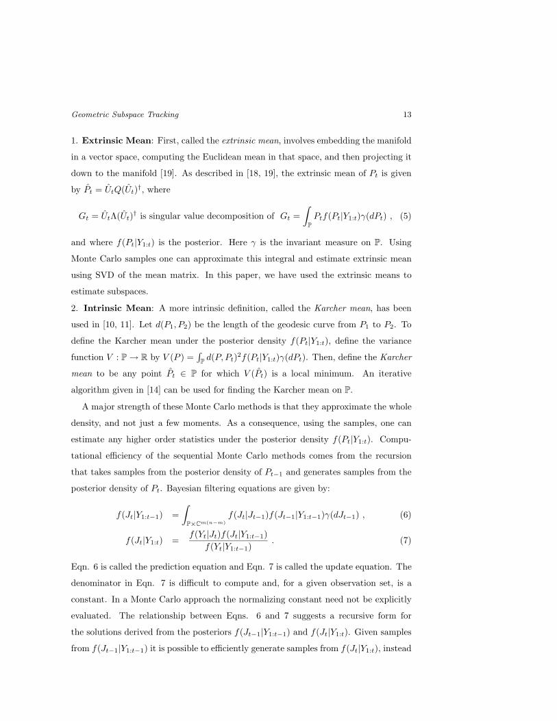
1. Extrinsic Mean: First, called the extrinsic mean, involves embedding the manifold
in a vector space, computing the Euclidean mean in that space, and then projecting it
down to the manifold [19]. As described in [18, 19], the extrinsic mean of Pt is given
by Pt = UtQ(Ut)†, where
Gt = UtΛ(Ut)† is singular value decomposition of Gt =∫
P
Ptf(Pt|Y1:t)γ(dPt) , (5)
and where f(Pt|Y1:t) is the posterior. Here γ is the invariant measure on P. Using
Monte Carlo samples one can approximate this integral and estimate extrinsic mean
using SVD of the mean matrix. In this paper, we have used the extrinsic means to
estimate subspaces.
2. Intrinsic Mean: A more intrinsic definition, called the Karcher mean, has been
used in [10, 11]. Let d(P1, P2) be the length of the geodesic curve from P1 to P2. To
define the Karcher mean under the posterior density f(Pt|Y1:t), define the variance
function V : P→ R by V (P ) =∫
Pd(P, Pt)2f(Pt|Y1:t)γ(dPt). Then, define the Karcher
mean to be any point Pt ∈ P for which V (Pt) is a local minimum. An iterative
algorithm given in [14] can be used for finding the Karcher mean on P.
A major strength of these Monte Carlo methods is that they approximate the whole
density, and not just a few moments. As a consequence, using the samples, one can
estimate any higher order statistics under the posterior density f(Pt|Y1:t). Compu-
tational efficiency of the sequential Monte Carlo methods comes from the recursion
that takes samples from the posterior density of Pt−1 and generates samples from the
posterior density of Pt. Bayesian filtering equations are given by:
f(Jt|Y1:t−1) =∫
P×Cm(n−m)f(Jt|Jt−1)f(Jt−1|Y1:t−1)γ(dJt−1) , (6)
f(Jt|Y1:t) =f(Yt|Jt)f(Jt|Y1:t−1)
f(Yt|Y1:t−1). (7)
Eqn. 6 is called the prediction equation and Eqn. 7 is called the update equation. The
denominator in Eqn. 7 is difficult to compute and, for a given observation set, is a
constant. In a Monte Carlo approach the normalizing constant need not be explicitly
evaluated. The relationship between Eqns. 6 and 7 suggests a recursive form for
the solutions derived from the posteriors f(Jt−1|Y1:t−1) and f(Jt|Y1:t). Given samples
from f(Jt−1|Y1:t−1) it is possible to efficiently generate samples from f(Jt|Y1:t), instead

14 Srivastava and Klassen
of directly sampling from f(Jt|Y1:t), which may be complicated and computationally
expensive. f(Jt|Jt−) is given in Section 3.1 and f(Yt|Jt) is given in Section 3.2. The
algorithm will be based on: (i) samples from the prior f(Jt|Jt−1) for a given value of
Jt−1, and (ii) the functional form of the density function f(Yt|Jt).
4.2. Sequential Monte Carlo Approach
A recursive formulation, which takes samples from f(Jt−1|Y1:t−1) and generates
the samples from f(Jt|Y1:t) in an efficient fashion, is desirable. Assume that, at the
observation time t − 1, we have a set St−1 = J (i)t−1 : i = 1, 2, . . . , M , J
(i)t−1 ∼
f(Jt−1|Y1:t−1). Following are the steps to generate the set St.
1. Prediction: The first step is to sample from f(Jt|Y1:t−1) given the samples
from f(Jt−1|Y1:t−1). We take a compositional approach by treating f(Jt|Y1:t−1) as
a mixture density. According to Eqn. 6, f(Jt|Y1:t−1) is the integral of the product of
a marginal and a conditional density. This implies that, for each element J(i)t−1 ∈ St−1,
by generating a sample from the conditional, f(Jt|J (i)t−1), we can generate a sample
from f(Jt|Y1:t−1) (see Algorithm 1). Now we have samples J (i)t from f(Jt|Y1:t−1);
analogous to Kalman-filtering these samples are called predictions.
2. Resampling: Given these predictions, the next step is to generate samples from
the posterior f(Jt|Y1:t). For this, we utilize importance sampling as follows. The
samples from the prior (f(Jt|Y1:t−1)) are resampled (see reference [15]) according to
the probabilities that are proportional to the likelihoods f(Yt|J (i)t ). Form a discrete
probability mass function on the set J (i)t : i = 1, 2, . . . , M:
βt,i =f(Yt|J (i)
t )∑Mj=1 f(Yt|J (j)
t ), and set βt = [βt,1 βt,2 . . . βt,M ] . (8)
Then, resample M values from the set J (1)t , J
(2)t , . . . , J
(M)t according to probability
βt. These values are the desired samples from the posterior f(Jt|Y1:t). Denote the
resampled set by St = J (i)t : i = 1, 2, . . . , M, J
(i)t ∼ f(Jt|Y1:t). It must be
remarked that after resampling, the indices (i) are renamed so that the sequence
J(i)t−1, J
(i)t , J
(i)t+1, . . . , for the same i, may not be consistent anymore. In other words,
it is possible that the velocity A(i)t−1 does not take P
(i)t−1 to P
(i)t in a unit time. This
inconsistency has no bearing on the estimation procedure since the past samples are
not used in estimating future parameters, only the current samples are used.

Geometric Subspace Tracking 15
3. Mean Estimation: Now that we have M samples from the posterior f(Jt|Y1:t), we
can average them appropriately to approximate the posterior mean of Pt. As described
in the paper [18], the extrinsic mean estimate of Pt is given by Eqn. 5. Using Monte
Carlo sampling, we approximate Gt by
Gt,M =1M
M∑i=1
P(i)t ∈ C
n×n, and compute SVD of Gt,M to obtain Pt,M . (9)
In numerous papers, the ergodic properties of sequential Monte Carlo samples have
been studied. It has been shown that the elements of the set St are exact samples
from the posterior and the ergodic property (that is, sample averages converge to the
expected values as the sample size gets larger) holds. It should be noted that due to
the resampling step, the resulting samples are not independent any more.
Error Analysis: There are two sources of error: (i) a sampling error in estimating
Gt by a finite sample mean Gt,M (this error is estimated using the sample variance
[19]), and (ii) there is a difference between the underlying true value Pt and its exact
posterior mean (this error is quantified using Hilbert-Schmidt lower bounds [18] that
are achieved by the estimator defined in Eqn. 5).
4.3. Subspace Tracking Algorithm
Given the samples J (i)t−1 : i = 1, 2, . . . , M ∼ f(Jt−1|Y1:t−1), the following steps
generate samples from posterior at time t and estimate Pt,M .
Algorithm 2. 1. Sample Conditional: Draw J (i)t , i = 1, . . . , M from the condi-
tional prior according to Algorithm 1.
2. Importance Weights: Compute probabilities β(i)t , i = 1, . . . , M , using Eqn. 8.
3. Resampling: Generate M samples from the set J (i)t , i = 1, . . . , M with proba-
bilities β(i)t , i = 1, . . . , M. Denote these samples by J (i)
t , i = 1, . . . , M.4. Mean Estimation: Calculate the sample average Gt,M according to Eqn. 9 and
compute the estimate Pt,M using the SVD of Gt,M . Set t← t + 1 and go to step 1.
5. Simulation Results
Now we present some experimental results on subspace tracking. Consider the
problem of subspace estimation using a uniform linear array of sensors with model as
16 Srivastava and Klassen
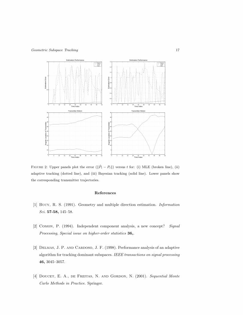
stated in Section 3.2. For these experiments, the transmitter motion is generated using
a simple auto-regressive model. The lower panels of Figure 2 show the trajectories
of two signal transmitters (m = 2). For each θt = [θ1,t, θ2,t], we generated yi,t for
n = 4 according to the sensor model and computed the sample covariance matrix Kt
according to Eqn. 1. The tracking algorithm then estimates Pt,M for M = 500 at each
time t.
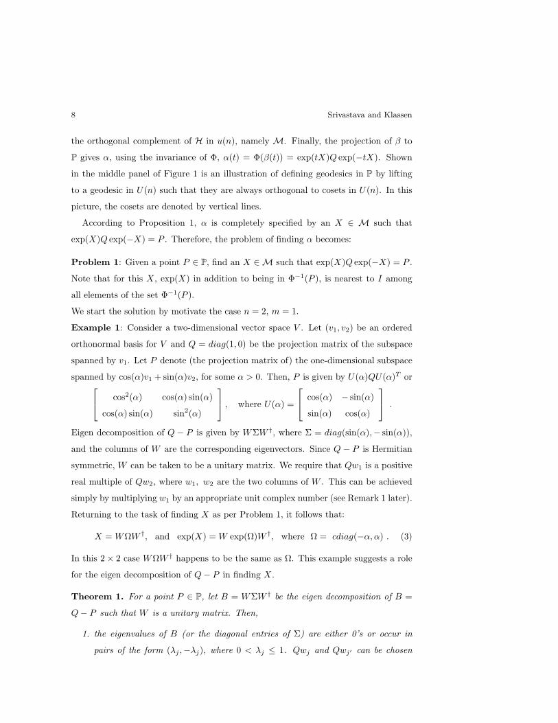
In Figure 2, each top panel shows the estimation error ‖Pt − P‖ for three different
estimation procedures. First, the error associated with the instantaneous maximum-
likelihood estimate (MLE), obtained by SVD of the covariance matrix Kt, is shown in
the broken line. The error resulting from an adaptive procedure, relying on the SVD
of the matrix Rt = γKt + (1− γ)Kt−1, is shown in the dotted line (for γ = 0.3). Note
that this choice of γ is arbitrary and the literature provides techniques for selecting
a better γ. Finally, the estimation error for tracking resulting from Algorithm 2 is
plotted in bold. Since the prior is based on a velocity model, MLEs at t = 1, 2 are used
to initialize the algorithm and Bayes’ inference starts at t = 3. As the theory suggests,
a prior model on subspace motion improves tracking performance in the presence of
intermittent noise. Algorithm 2 estimates only the current state and gains in speed by
not improving upon the past estimates. A slower algorithm for joint estimation of all
the states, using all the observations, is given in [16].
6. Summary
In this paper, we have proposed a Bayesian approach to tracking principal subspaces
using observations taken from time-varying systems. A prior model, on stochastic
process on a Grassmann manifold, is used to formulate the Bayesian problem. A re-
cursive, computational technique to sample from the posterior and to generate Bayesian
estimates is described.
Acknowledgements
This research was supported by ARO DAAG55-98-1-0102, ARO DAAD19-99-1-0267
and NSF DMS0101429. We thank the anonymous referee for helpful comments.
Geometric Subspace Tracking 17
0 5 10 15 20 25 30 35 40 45 500
0.5
1
1.5
Est
imat
ion
Err
or
Time Index
Estimation Performance
BayesConv MLE
0 5 10 15 20 25 30 35 40 45 500
0.2
0.4
0.6
0.8
1
1.2
1.4
1.6
Est
imat
ion
Err
orTime Index
Estimation Performance
BayesConv MLE
0 5 10 15 20 25 30 35 40 45 505
10
15
20
25
30
35
40
45
50Transmitter Motion
Time Index
Ang
ular
Loc
atio
n of
Tra
nsm
itter
0 5 10 15 20 25 30 35 40 45 500
5
10
15
20
25
30
35
40
45Transmitter Motion
Time Index
Ang
ular
Loc
atio
n of
Tra
nsm
itter
Figure 2: Upper panels plot the error (‖Pt − Pt‖) versus t for: (i) MLE (broken line), (ii)
adaptive tracking (dotted line), and (iii) Bayesian tracking (solid line). Lower panels show
the corresponding transmitter trajectories.
References
[1] Bucy, R. S. (1991). Geometry and multiple direction estimation. Information
Sci. 57-58, 145–58.
[2] Comon, P. (1994). Independent component analysis, a new concept? Signal
Processing, Special issue on higher-order statistics 36,.
[3] Delmas, J. P. and Cardoso, J. F. (1998). Performance analysis of an adaptive
algorithm for tracking dominant subspaces. IEEE transactions on signal processing
46, 3045–3057.
[4] Doucet, E. A., de Freitas, N. and Gordon, N. (2001). Sequential Monte
Carlo Methods in Practice. Springer.
18 Srivastava and Klassen
[5] Edelman, A., Arias, T. and Smith, S. T. (1998). The geometry of algorithms
with orthogonality constraints. SIAM Journal of Matrix Analysis and Applications
20, 303–353.
[6] Gordon, N. J., Salmon, D. J. and Smith, A. F. M. (1993). A novel approach
to nonlinear/non-gaussian bayesian state estimation. IEEE Proceedings on Radar
Signal Processing 140, 107–113.
[7] Helgason, S. (1978). Differential Geometry, Lie Groups and Symmetric Spaces.
Academic Press.
[8] Jolliffe, I. T. (1986). Principal component analysis. Springer series in statistics.
Springer-Verlag.
[9] Jupp, P. E. and Kent, J. T. (1987). Fitting smooth paths to spherical data.
Applied Statistics 36, 34–46.
[10] Karcher, H. (1977). Riemann center of mass and mollifier smoothing.
Communications on Pure and Applied Mathematics 30, 509–541.
[11] Kendall, W. S. (1990). Probability, convexity, and harmonic maps with small
image I: Uniqueness and fine existence. Proceedings of the London Mathematical
Society 61, 371–406.
[12] Kobayashi, S. and Nomizu, K. (1969). Foundations of Differential Geometry,
vol 2. Interscience Publishers.
[13] Le, H. (1991). On geodesics in euclidean shape spaces. J. Lond. Math. Soc. 44,
360–372.
[14] Le, H. (2001). Locating frechet means with application to shape spaces. Advances
in Applied Probability 33, 324–338.
[15] Liu, J. S. and Chen, R. (1998). Sequential monte carlo methods for dynamic
systems. Journal of the American Statistical Association 93, 1032–44.
[16] Miller, M. I., Srivastava, A. and Grenander, U. (1995). Conditional-
expectation estimation via jump-diffusion processes in multiple target track-
ing/recognition. IEEE Transactions on Signal Processing 43, 2678–2690.
Geometric Subspace Tracking 19
[17] Schmidt, R. (Nov. 1981). A signal subspace approach to multiple emitter location
and spectral estimation. Ph.D. Dissertation of Stanford University, Palo Alto, CA.
[18] Srivastava, A. (2000). A bayesian approach to geometric subspace estimation.
IEEE Transactions on Signal Processing 48, 1390–1400.
[19] Srivastava, A. and Klassen, E. (2001). Monte carlo extrinsic estimators for
manifold-valued parameters. IEEE Trans. on Signal Processing 50, 299–308.
[20] Tong, L. and Perreau, S. (1998). Multichannel blind estimation: From
subspace to maximum likelihood methods. Proc. of the IEEE 86, 1951–1968.
[21] Warner, F. W. (1994). Foundations of Differentiable Manifolds and Lie Groups.
Springer-Verlag, New York.
A. Proof of Theorem 1
Let P and Q be two m-dimensional subspaces of V , with projection matrices P and
Q, respectively. We will prove the theorem in three steps: (i) prove the case n = 2
and m = 1, (ii) show that if there exists a basis of V such that P = exp(Ω)Q for a
specific Ω ∈ M, then the theorem is just an extension of the n = 2, m = 1 case, and
(iii) for any given P , show that there exists a basis of V such that the requirements of
the second step are met.
1. Let n = 2 and m = 1, and rule out the cases Q ⊥ P and Q = P since they are easy
to handle. For v1 ∈ Q (‖v1‖ = 1), we have Pv1 ∈ P . Let w1 be the unit vector in P
such that w1 ·Pv1 > 0, and let α1 be the (positive) angle between v1 and w1. As shown
in Example 1, Q − P can be decomposed as W diag(λ1,−λ1) W † for λ1 = sin(α1).
The resulting X ∈M and exp(X) ∈ U(n) are given in Eqn. 3.
2. For arbitrary P ∈ P, we will essentially decompose V as orthogonal direct sum of
two-dimensional subspaces to obtain the best rotation from Q to P . Part 1 will apply
independently to each two-dimensional component. Let there be an orthonormal basis
of V of the form
(u1, . . . , uk, v1, . . . , vr, w1, . . . , wr, x1, . . . , xp) (10)
20 Srivastava and Klassen
where k, r, p are three nonnegative integers such that k + 2r + p = n and k + r = m.
Also, let (u1, . . . , uk, v1, . . . , vr) be an orthonormal basis of Q. For α1, . . . , αr ∈ R+ ,
define an element of u(n) by Ω = diag(0k,k, B, 0p,p) ∈ Rn×n, where B = cdiag(−C,C)
and C = diag(α1, . . . , αr). Define a subspace P = exp(Ω)Q. We can also write
P = spanu1, . . . , uk, cos(α1)v1 +sin(α1)w1, . . . , cos(αm)vm +sin(αm)wm. (u1, . . . uk)
is a basis of (Q ∩ P ), and (x1, . . . , xp) is a basis of the space Q⊥ ∩ P⊥. With respect
to the basis given in Eqn. 10, we can factor the rotation from Q to P into a sequence
of 2 × 2 rotations in 2-planes orthogonal to each other. The planes are spanned by
vj , wj and the rotation angles are αj ’s. The results from Part 1 apply to each 2 × 2
rotation independently. Therefore, the eigen decomposition of Q − P takes the form:
W diag(0k,k, B,−B, 0p,p) W † where B = diag(λ1, . . . , λr) and λj = sin(αj). Using
the 2 × 2 example, X = WΩW † is the desired X ∈ M, and exp(X) = W exp(Ω)W †.
Therefore, if there exists a basis of V of the type given in Eqn. 10 such that Q and P
can be written in these specific forms, the result follows from two-dimensional analysis.
Note that Ω here is a permutation of the Ω stated in Theorem 1. This is not an issue
as long as the columns of W are also permuted accordingly.
3. Next, we show that for any P ∈ P, there exists an orthonormal basis of V of the
form given in Eqn. 10. Let k = dim(Q ∩ P ) and p = dim(Q⊥ ∩ P⊥). Choose any
orthonormal bases u1, . . . , uk for Q ∩ P and x1, . . . , xp for Q⊥ ∩ P⊥.
Since all rotation will take place in the orthogonal complement of (Q∩P )⊕(Q+P )⊥,
we now replace V by the orthogonal complement in V of the subspace (Q ∩ P ) ⊕(Q + P )⊥, P by the orthogonal complement in P of P ∩ Q, and Q by the orthogonal
complement in Q of P ∩ Q. Now, dim(P ) = dim(Q) = r and dim(V ) = 2r; P ∩ Q = 0
and they span V . Let SP and SQ denote the unit spheres in P and Q, respectively
and let ε = inf|v − w| : v ∈ SQ and w ∈ SP . Since SP and SQ are disjoint compact
sets, ε > 0 and there exist vectors v ∈ SQ and w ∈ SP satisfying |v − w| = ε. We now
choose basis elements of Q and P as follows: Let v1 = v, and let w1 be the unique unit
vector in the real span of v, w such that (1) w1 ⊥ v and (2) w1 ·Pv > 0. To construct
the rest of the basis, inductively replace P , Q, and V by the orthogonal complement
of span(v, w) in each of them, and repeat this step to find (v2, w2), . . . , (vr, wr).
Related Documents


![Fetal ECG Subspace Estimation Based on Cyclostationarity · 2016. 9. 9. · approaches, such as Bayesian filter [7], Kalman filter [8] (specifically for linear model assumption),](https://static.cupdf.com/doc/110x72/5fe2f83e36218a2f820501e2/fetal-ecg-subspace-estimation-based-on-cyclostationarity-2016-9-9-approaches.jpg)


