Bayesian analysis of non-homogeneous Markov chains: Application to mental health data

BAYESIAN ANALYSIS OF NONHOMOGENEOUS MARKOV

CHAINS: APPLICATION TO MENTAL HEALTH DATA

Minje Sung , Refik Soyer , Nguyen Nhan"‡ # $

"Department of Biostatistics and Bioinformatics, Box 3454, Duke University Medical

Center, Durham, NC 27710, USA.2Department of Management Science, The George Washington University, Washington,

DC 20052, USA.3Research Director (now retired), Graydon Manor Psychiatric Center, Leesburg, VA,

USA.

*Corresponding author: Tel +1 919 687 4686, x-294; fax + 1 919 687 4737; e-mail

[email protected].

1

SUMMARY

In this paper we present a formal treatment of nonhomogeneous Markov chains

by introducing a hierarchical Bayesian framework. Our work is motivated by the analysis

of correlated categorical data which arise in assessment of psychiatric treatment

programs. In our development, we introduce a Markovian structure to describe the

nonhomogeneity of transition patterns. In so doing, we introduce a logistic regression

setup for Markov chains and incorporate covariates in our model. We present a Bayesian

model using Markov chain Monte Carlo methods and develop inference procedures to

address issues encountered in the analyses of data from psychiatric treatment programs.

Our model and inference procedures are implemented to some real data from a

psychiatric treatment study.

Key words: Markov models, Bayesian inference, longitudinal data, dynamic models.

1. Introduction

Categorical type longitudinal data often arises in studies of psychiatric treatment

programs where measurements describe either the mental status of the patients or their

functioning status in the program at different points in time. Modeling the states of the

subjects over time, understanding the changing behavior of the patients and related

analyses are of interest to scientists who are involved in these studies. Nhan [1] presented

an example of data from a psychiatric treatment study of children and young adolescents

and discussed such issues of interest. In modeling this type of data, the states measured at

discrete points in time are considered as a sequence of correlated discrete random

variables. Thus, a Markov chain is typically used to describe the correlation structure. An

earlier example of this is the homogeneous Markov chain model proposed by Meredith

[2] for evaluation of a treatment program. However, the analysis of this type of data from

treatment programs often suggests nonhomogeneous transition patterns for patients. For

example, in his study Nhan [1] observed strong evidence in favor of nonhomogeneity in

transition probabilities for patients.

In this paper we present a formal treatment of nonhomogeneous Markov chains

by introducing a hierarchical Bayesian framework. In the Bayesian literature, the term

Markov model may be used to refer to two different classes of models which can be

classified as and Markov models using theparameter driven observation driven

terminology of Cox [3]. Both of these models are used for categorical time series data.

The observation driven Markov models are the Markov chains where the Markov

structure is on the observables such as the state occupancies of the individuals. As

pointed out by Erkanli et al. [4], most of the work in Bayesian literature concentrated on

the parameter driven Markov models such as Cargnoni et al. [5] where the parameters

evolve over time according to a first-order Markov model. These models are in the same

class as the dynamic linear models (DLM's) of Harrison and Stevens [6] and general

DLM's of West et al. [7]. Even though he t models are notparameter driven Markov

3

Markov chains, they are of interest to us in modeling transition matrices for our analysis

of nonhomogeneous Markov chains.

Earlier efforts to make inferences on the transition probabilities of a Markov

chain can be found in Anderson and Goodman [8] where the maximum likelihood

methods are used and in Lee et al. [9] where a Bayesian analysis of the homogeneous

Markov chains is presented using a Dirichlet prior distribution on transition probabilities.

An empirical Bayes approach is introduced by Meshkani [10] for homogenous chains

who considered extensions to nonhomogeneous Markov chains by viewing the problem

as a parametric empirical Bayes problem in the sense of Morris [11]. These earlier

approaches have not considered the effects of covariates on transition probabilities.

Muenz and Rubinstein [12] presented a logistic regression setup for a binary

Markov chain, and obtained the maximum likelihood estimates for the transition

probabilities. Zeger and Qaqish [13] presented the Markov logistic regression setup for

correlated longitudinal data and discussed maximum likelihood estimation (MLE) for the

model. This setup fits into the transition models of Diggle et al. [14] where the

Markovian structure on the observations is introduced via the logistic link function.

Recently, Erkanli et al. [4] pointed out some of the problems in applying MLE methods

in Markov logistic regression setup with only a few number of observations and

presented Bayesian methods. However, the work of Erkanli et al. [4] is based on binary

Markov logistic regression models and their treatment of nonhomogeneity is via

inclusion of time dependent deterministic covariates.

In this paper we present Bayesian methods for modeling and analyses of

nonhomogeneous Markov chains, and develop inference procedures to be able to address

issues encountered in the analyses of data from psychiatric treatment programs. In so

doing, we introduce a class of models for describing nonhomogeneity in the transition

probabilities. MuenzOur modeling strategy is based on the logistic regression setup of

and Rubinstein [12] and uses a Markovian structure for describing time evolution of

4

Markov chain's transition matrix. Thus, in the sense of Cox [3], our models can be

classified as and Markov models.parameter observation driven

In section 2, we present a hierarchical Bayes representation of the static logistic

regression setup for homogeneous Markov chains. We extend our setup by introducing a

first order Markov structure for describing the time dependence of transition probabilities

of the nonhomogeneous Markov chains. Bayesian inferences for these models are fully

developed in section 3. In section 4, the models are applied to real data from a psychiatric

treatment program and conclusions are presented in section 5.

2. Models for Nonhomogeneous Markov Chains

In this section, we present the Markov chain model and introduce a hierarchical

Bayesian representation of the logistic regression setup for Markov chains. We first

present the Markov chains andhierarchical Bayesian representation for homogeneous

then introduce a dynamic Markovian modeling strategy for describing uncertainty about

transition probabilities of nonhomogeneous Markov chains.

2.1. Notation and preliminaries

Define as a sequence of random variables indexed by timeÖ= ß = ß = ß ÞÞÞ×7! 7" 7#

taking finite values in . We assume that the sequence X œ Ö"ß ÞÞÞß N × Ö= ß = ß = ß ÞÞÞ×7! 7" 7#

forms a first-order Markov chain as the conditional probability distribution of given=7>

= ßá ß = = =7ß>" 7! 7ß>" 7> depends only on the value of . Here, represents the state of a

patient at time Let represent the transition of the -th individual from state at7 >Þ B 7 3734>

time to state at time , that is,Ð> "Ñ 4 >

B œ "Ð= œ 4l= œ 3Ñß734> 7> 7ß>" (1)

where 1 takes the value if event occurs and otherwise. Then, the vectorÐEÑ " E !

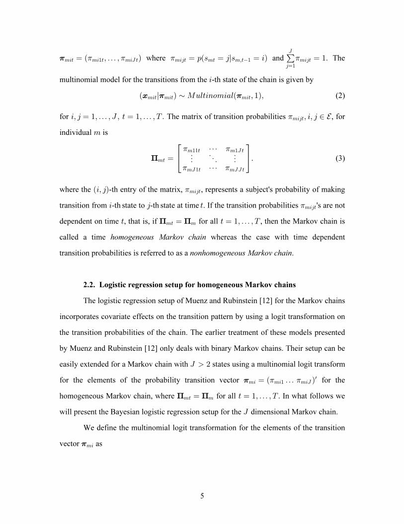
B73> 73"> 73N >œ ÐB ßá ß B Ñ is a multinomial random variable with probability vector

5

173> 73"> 73N > 734> 7> 7ß>" 734>4œ"

N

œ Ð ßá ß Ñ œ :Ð= œ 4l= œ 3Ñ œ "1 1 1 1 where and . ! The

multinomial model for the transitions from the -th state of the chain is given by3

Ð l Ñ µ Q?6>38973+6Ð ß "ÑßB73> 73> 73>1 1 (2)

for 3ß 4 œ "ß ß N ß > œ "ß ß X Þá á ß 3ß 4 −The matrix of transition probabilities , for1 X734>

individual is7

C7>

7" > 7"N >

7N > 7NN>

ω

ã ä ãâ

Ô ×Õ Ø1 1

1 1

1

1

. (3)

where the -th entry of the matrix, , represents a subject's probability of makingÐ3ß 4Ñ 1734>

transition from -th state to -th state at time . 3 4 > If the transition probabilities 's are not1734>

dependent on time , that is, if for all , then the Markov chain is> > œ "ßá ß XC C7> 7œ

called a time whereas the case with time dependenthomogeneous Markov chain

transition probabilities is referred to as a .nonhomogeneous Markov chain

2.2. Logistic regression setup for homogeneous Markov chains

The logistic regression Muenz and Rubinstein [12] for the Markov chainssetup of

incorporates covariate effects on the transition pattern by using a logit transformation on

the transition probabilities of the chain. The earlier treatment of these models presented

by Muenz and Rubinstein [12] only deals with binary Markov chains. Their setup can be

easily extended for a Markov chain with states using a multinomial logit transformN #

for the elements of the probability transition vector for the173 73" 73Nwœ Ð á Ñ1 1

homogeneous Markov chain, where for all . In what follows weC C7> 7œ > œ "ßá ß X

will present the Bayesian logistic regression setup for the dimensional Markov chain.N

We define the multinomial logit transformation for the elements of the transition

vector as173

6

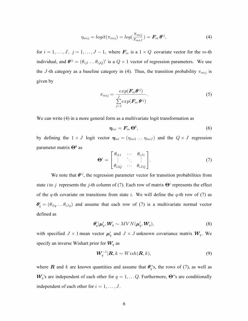
( 111734 734 7734

73N

34œ 6913>Ð Ñ œ 691Ð Ñ œ ßJ ) (4)

for , where is a covariate vector for the -th3 œ "ßá ß N ß 4 œ "ßá ß N " " ‚ U 7J7

individual, and is a vector of regression parameters. We use)34 wœ Ð Ñ) )34 34U1 á U‚ "

the -th category as a baseline category in (4). Thus, the transition probability isN 1734

given by

1734

4œ"

Nœ Þ

/B:Ð Ñ

/B:Ð Ñ

J

J

734

734

)

)!(5)

We can write (4) in a more general form as a multivariate logit transformation as

(73 7œ ßJ @3 (6)

by defining the logit vector regression" ‚ N ‚ N(73 73" 73Nœ Ð á Ñ U( ( and the

parameter matrix as@3

@3 ω

ã ä ãâ

Ô ×Õ Ø) )

) )

3" 3N"

3"U 3NU

1

. (7)

We note that )34, the regression parameter vector for transition probabilities from

state to represents the -th column of (7). Each row of matrix 3 4 4 @3 represents the effect

of the -th covariate on transitions from state . We will define the ; 3 ;-th row of (7) as

)3; œ Ð Ñ) )3"; 3N ;á and assume that each row of (7) is a multivariate normal vector

defined as

) . .3 3 3; ; ;; ;l ß µ QZ RÐ ß Ñß[ [ (8)

with specified mean vector N ‚ " .3; ; and unknown covariance matrix . WeN ‚ N [

specify an inverse Wishart prior for as[;

[ V V;"l ß 5 µ [3=2Ð ß 5Ñß (9)

where V and are known quantities and assume that 's, the rows of (7), as well as5 )3;

[; 's are independent of each other for . Furthermore, 's are conditionally ; œ "ßáU @3

independent of each other for .3 œ "ßá ß N

7

In summary, the logistic regression setup for homogeneous Markov chains can be

represented as a hierarchical Bayesian model as

B73> 73 73l µ Q?6>38973+6Ð ß "Ñ1 1 ,

( 1734 734 734œ 6913>Ð Ñ œ ßJ )

) . .3 3 3; ; ;; ;l ß µ QZ RÐ ß Ñß[ [

[ V V;"l ß 5 µ [3=2Ð ß 5Ñ. (10)

The hierarchical setup (10) associated with the th row of the transition matrix is3 C7

generalized to include , , that is, at the first level of the hierarchy, 's are3 œ "ßá N B73

independent given 's for At the second level, 's are conditionally1 173 733 Á 4Þ

independent for . The unknown quantities that are common for all 's, will3 Á 4 3[; ,

induce some form of dependence across the rows of the transition probability matrix. The

Bayesian analysis of the hierarchical model (10) will be presented in Section 3.

2.3. Models for nonhomogeneous Markov chains

described in the previousThe logistic regression setup of the Markov chain

section is an observation driven Markov model. We next extend the hierarchical

Bayesian representation given by (10) to the nonhomogeneous Markov chains. We note

that the time nonhomogeneity of transition probabilities can be incorporated into the

model by using time dependent covariates J7> in (4). However, in what follows, we

consider a formal treatment of nonhomogeneity by introducing a Markovian structure to

describe the evolution of transition probabilities over time. The resulting models can be

classified as parameter and observation driven Markov models.

In our development we consider the regression parameter matrix of (7) and index

it by time as

.@>3 œ

âã ä ã

â

Ô ×Õ Ø) )

) )

3" > 3N">

3"U> 3NU>

1

(11)

8

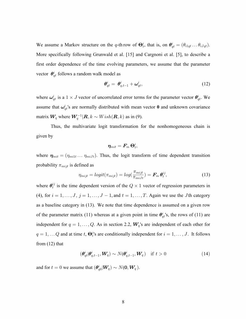
We assume a Markov structure on the , that is, on ; œ Ð Ñ-th row of .@>3 )3

;> ) )3";> 3N ;>á

More specifically following Grunwald et al. [15] and Cargnoni et al. [5], to describe a

first order dependence of the time evolving parameters, we assume that the parameter

vector follows a random walk model as)3;>

) )3 3;> ;ß>"œ =3

;>ß (12)

where is a vector of uncorrelated error terms for the parameter vector . We=3;> " ‚ N )3

;>

assume that 's are normally distributed with mean vector and unknown covariance=3;> 0

matrix [ [ V V; ; where as in (9). "l ß 5 µ [3=2Ð ß 5Ñ

Thus, the multivariate logit transformation for the nonhomogeneous chain is

given by

(73> 7œ ßJ @>3

where (73> 73"> 73N >œ Ð á Ñ( ( . Thus, the logit transform of time dependent transition

probability 1734> is defined as

( 111734> 734> 7734>

73N >

34>œ 6913>Ð Ñ œ 691Ð Ñ œ ßJ ) (13)

where )34> is the time dependent version of the vector of regression parameters inU‚ "

(4), for , and . Again we use the th category3 œ "ßá ß N ß 4 œ "ßá ß N " > œ "ßá ß X N

as a baseline category in (13). We note that time dependence is assumed on a given row

of the parameter matrix (11) whereas at a given point in time )3;>'s, the rows of (11) are

independent for . As in section 2.2, 's are independent of each other for; œ "ßá ßU [;

; œ "ßáU > 3 œ "ßá ß N and at time , 's are conditionally independent for . @>3 It follows

from (12) that

Ð ß Ñ µ R ß Ñ > ! Ð Ñ) ) )3 3 3;> ;ß>" ;ß>"| ( if 14[ [; ;

and for we assume that | ( .> œ ! Ð Ñ µ R ß Ñ)3;! [ [; ;!

9

Thus, the logistic regression setup for nonhomogeneous Markov chains can be

represented as a hierarchical Bayesian model as

B73> 73> 73>l µ Q?6>38973+6Ð ß "Ñ1 1 ,

( 1734> 734> 734>œ 6913>Ð Ñ œ ßJ )

) ) )3 3 3;> ;ß>" ;ß>"| (ß µ R ß Ñ[ [; ; ß

[ V V !; ;!3"l ß 5 µ [3=2Ð ß 5Ñ and ) | ( .[ [; ;µ R ß Ñ (15)

The hierarchical Bayes setup (15) is associated with the th row of the transition matrix3

C7> in (3). It can be generalized to include , , that is, at the first level of the3 œ "ß á N

hierarchy, 's are independent given 's for As before at the second level,B73> 73>1 3 Á 4Þ

173>'s are conditionally independent for . As in the homogeneous case, (15)3 Á 4

represents the hierarchical setup for individual .7

3. Posterior Analysis of Markov Chain Models

We consider the hierarchical Bayesian representations given by (10) and (15) for

homogeneous and nonhomogeneous Markov chain models. We note that the hierarchical

Bayesian setups are shown for the transitions from the -th state of the Markov chain for3

a specific individual . The generalization of the setup to all states, , for 7 3 œ "ß ÞÞÞß N Q

individuals, , is straightforward due to the conditional independence of7 œ "ß ÞÞÞßQ

B73> 73 73>'s given the transition probability vectors 's and 's. In what follows, we will1 1

present the Bayesian analyses of both homogeneous and nonhomogeneous Markov chain

models.

3.1. Posterior analysis for homogeneous chains

Given the transition data on individuals for time periods, the joint posteriorQ X

distribution needed for the Bayesian analysis of homogeneous Markov chains is

10

:Ð ß ß ß ß l ß ÞÞÞß ÑC C" Q " Qá ßáß@ @" N [ [" Ußá ß W W

º :Ð l Ñ :Ð l ß Ñ:Ð Ñ$$ $ $” •7œ"3œ" >œ" ;œ"

Q N X

73>

U

B @3 ) .3 3; ; [ [; ; , (16)

where the components of represents the transition matrix of the -th subject,C7 7

W W" Qß ß Q > œ "ß ß Xá á are the observed transitions of individuals over time periods,

with . Since the joint posterior distribution in (16) can not beW7 7! 7Xœ Ö= ß ß = ×á

obtained in any analytically tractable form, we will use a Gibbs sampler to draw samples

from the full conditional distributions:

Ð l ß Ñß Ð l ß Ñ@ @3 3W WÐÑ ÐÑ[ [; ; , (17)

where ) and for notational convenience, we denote the full conditionalW œ ÐW W" Qß ÞÞÞß

posterior distribution of a random quantity by where includes all9 9 9 9:Ð l ÑWß ÐÑ ÐÑ

random quantities except .9

For simulating , the matrix of the regression parameters in (7), we can@3 U‚ N

write

:Ð l ß Ñ º :Ð l Ñ :Ð l ß Ñ@ @ @3 3 3W BÐÑ

7œ" >œ" ;œ"

Q X

73>

U$ $ $” • ) .3 3; ; [; , (18)

which can be rewritten as proportional to

$$$ "Œ !7œ">œ" 4œ" ;œ"

Q X N

4œ"

N

B Uw

/B:Ð Ñ

/B:Ð Ñ

/B:Ö Ð Ñ Ð Ñ×"

#

J

J

734

734

3 3 3 3; ; ; ;

)

)

) . ) .734>

[ "; (19)

which is not a known density form. However, it can be shown that (19) is log-concave in

@3; see Appendix A for details and we can use the adaptive rejection sampling algorithm

of Gilks and Wild [16].

To draw from :Ð[ [ [; ; ;l ß ÑW ÐÑ , we note that the full conditional of can be"

written as

11

º l l /B:Ö >< Ð ß"

#W W; ;

" "Ð5NÑÎ# ˆ ‰ ‘V ) . ) .3 3 3 3; ; ; ;Ñ Ð Ñ

w

(20)

which is a Wishart density with degree of freedom, and scale matrix5 N "ß

"#ˆ ‰V Ð ) . ) .3 3 3 3

; ; ; ;Ñ Ð Ñ Þ w

3.2. Posterior analysis for nonhomogeneous chains

or theGiven the transition data on individuals for time periods, fQ X

nonhomogeneous Markov chains setup, we need to obtain the joint posterior distribution

:Ð Þ ß ß ß l ß ÞÞÞß ÑC C"" QX " Q, á ß áß@ @" X" N [ [" Ußá ß W W

º :Ð l Ñ :Ð l ß Ñ:Ð Ñ$$$ $7œ"3œ" >œ" ;œ"

Q N X

73>

U

B @>3 ) )3 3

;> ;ß>" [ [; ; . (21)

For simulating , we can use the Markov property as implied by (12) and write@>3

:Ð l ß Ñ º :Ð l Ñ :Ð l ß Ñ:Ð l ß Ñ@ @ @> > >3 3 3W B

ÐÑ

7œ" ;œ"

Q

73>

U$ $ ) ) ) )3 3 3 3;> ;ß>" ;ß>" ;>[ [; ; , (22)

implying that is:Ð l ß Ñ@ @> >3 3W

ÐÑ

º /B: Ð Ñ Ð Ñ"

#$ $ "’ “ ’ Š7œ" 4œ" ;œ"

Q N

734>B

Uw1 734> ) ) ) )3 3 3 3

;> ;ß>" ;> ;ß>"[ ";

Ð Ñ Ð Ñ) ) ) )3 3 3 3;ß>" ;> ;ß>" ;>

w[ "; ‹“. (23)

Note that the conditional posterior distribution of has a similar form as in (19) except@>3

that the product with respect to the time index is suppressed. Thus, it can be shown thatt

(23) is a log concave density and we can use the adaptive rejection sampling algorithm to

draw @>3 's .

To draw from :Ð[ [ [; ; ;l ß ÑW ÐÑ , we note that the full conditional of can be"

written as proportional to

12

l l /B: >< Ð ÑÐ Ñ"

#W; ;

" Ð5XN"ÑÎ#

>œ"

X’ šŠ ‹ “"V ) ) ) )3 3 3 3;> ;ß>" ;> ;ß>"

w

[ "› ,

(24)

which is again a Wishart density with degree of freedom, and scale matrix5 X N ß

Š ‹!V >œ"

X

Ð ÑÐ Ñ Î) ) ) )3 3 3 3;> ;>;ß>" ;ß>"

w

2Þ

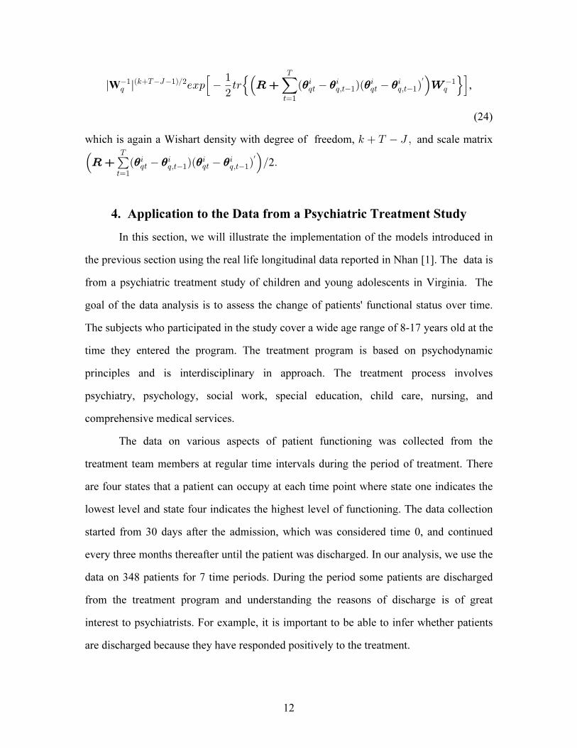
4. Application to the Data from a Psychiatric Treatment Study

In this section, we will illustrate the implementation of the models introduced in

the previous section using the real life longitudinal data reported in Nhan [1]. The data is

from a psychiatric treatment study of children and young adolescents in Virginia. The

goal of the data analysis is to assess the change of patients' functional status over time.

The subjects who participated in the study cover a wide age range of 8-17 years old at the

time they entered the program. The treatment program is based on psychodynamic

principles and is interdisciplinary in approach. The treatment process involves

psychiatry, psychology, social work, special education, child care, nursing, and

comprehensive medical services.

The data on various aspects of patient functioning was collected from the

treatment team members at regular time intervals during the period of treatment. There

are four states that a patient can occupy at each time point where state one indicates the

lowest level and state four indicates the highest level of functioning. The data collection

started from 30 days after the admission, which was considered time 0, and continued

every three months thereafter until the patient was discharged. In our analysis, we use the

data on 348 patients for 7 time periods. During the period some patients are discharged

from the treatment program and understanding the reasons of discharge is of great

interest to psychiatrists. For example, it is important to be able to infer whether patients

are discharged because they have responded positively to the treatment.

13

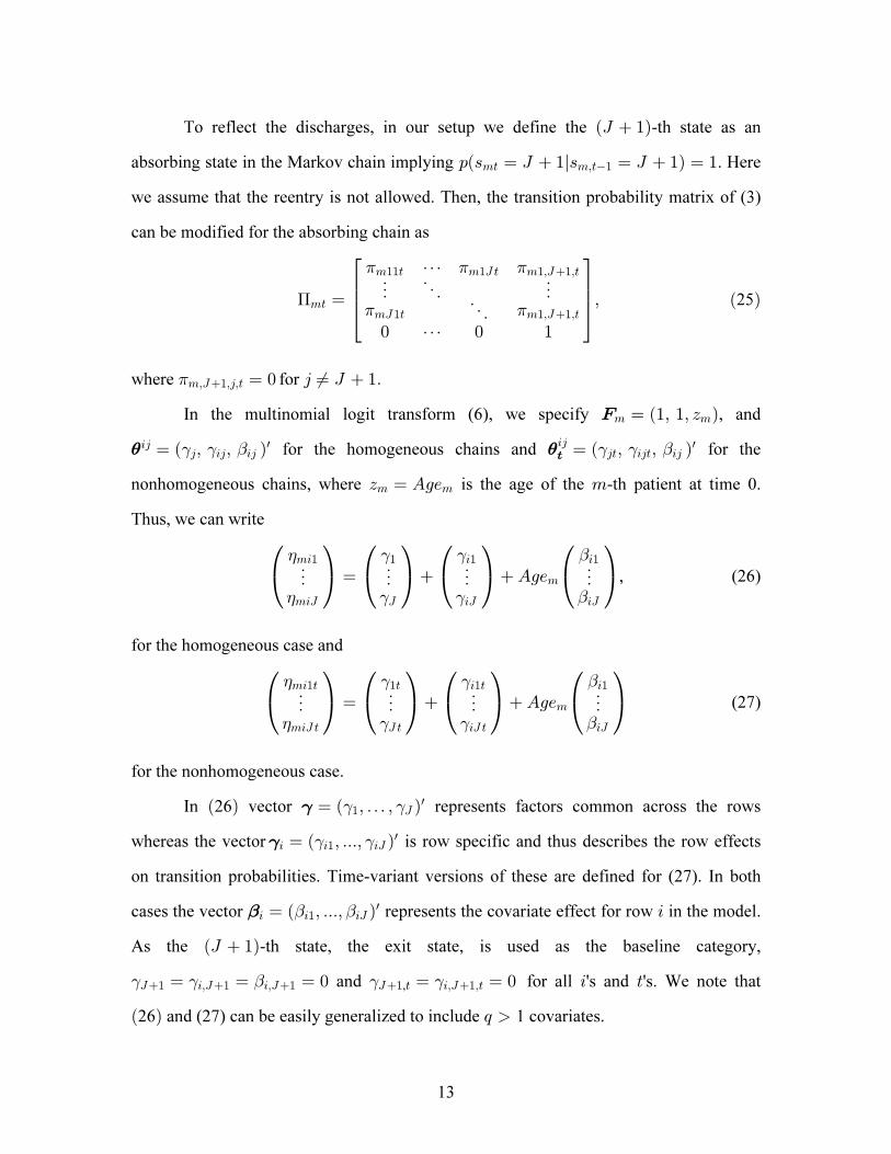
To reflect the discharges, in our setup we define the -th state as anÐN "Ñ

absorbing state in the Markov chain implying . Here:Ð= œ N "l= œ N "Ñ œ "7> 7ß>"

we assume that the reentry is not allowed. Then, the transition probability matrix of (3)

can be modified for the absorbing chain as

C

1 1 1

1 17>

7""> 7"N > 7"ßN"ß>

7N"> 7"ßN"ß>œ ß Ð Ñ

âã ä ã

ä! â ! "

Ô ×Ö ÙÖ ÙÕ Ø

25

where for 17ßN"ß4ß> œ ! 4 Á N "Þ

In the multinomial logit transform (6), we specify J7 7œ Ð"ß "ß D Ñ, and

) )34 w w4 34 34 4> 34> 34

34œ Ð ß ß Ñ œ Ð ß ß Ñ# # " # # " for the homogeneous chains and for the>

nonhomogeneous chains, where is the age of the -th patient at time 0.D œ E1/ 77 7

Thus, we can write

Î Ñ Î Ñ Î Ñ Î ÑÏ Ò Ï Ò Ï Ò Ï Ò

( # # "

( # # "

73" " 3" 3"

73N N 3N 3N

7ã ã ã 㜠E1/ , (26)

for the homogeneous case and

Î Ñ Î Ñ Î Ñ Î ÑÏ Ò Ï Ò Ï Ò Ï Ò

( # # "

( # # "

73"> "> 3"> 3"

73N > N > 3N > 3N

7ã ã ã 㜠E1/ (27)

for the nonhomogeneous case.

In 26 vector represents factors common across the rowsÐ Ñ œ Ð ßá ß Ñ# # #" Nw

whereas the vector is row specific and thus describes the row effects#3 3" 3Nwœ Ð ß ÞÞÞß Ñ# #

on transition probabilities. Time-variant versions of these are defined for (27). In both

cases the vector "3 3" 3Nwœ Ð ß ÞÞÞß Ñ 3" " represents the covariate effect for row in the model.

As the -th state, the exit state, is used as the baseline category,ÐN "Ñ

# # " # #N" 3ßN" 3ßN" N" > 3ßN"ß>œ œ œ ! œ œ ! 3 > and for all 's and 's. We note that,

Ð Ñ ; 26 and (27) can be easily generalized to include 1 covariates.

14

4.1. Prior distributions for logistic parameters

In describing prior uncertainty about the unknown model parameters, in all cases

we used non-informative but proper priors. More specifically, in the homogeneous

Markov chain multivariate normal distributions for parameterwe assume independent

vectors and # # "ß ß3 3. In each of the multivariate normal distributions, we specified zero-

mean vectors and the unknown precision matrices, In all cases the scale matrix of theV

Wishart was assumed to be implying a high degree of.3+1ÐÞ!"ß Þ!"ß Þ!"ß Þ!"Ñ

uncertaintyÞ

In the non modelhomogeneous Markov chain , for time homogeneous parameters

we used the same priors as given above for the homogeneous case. MarkovianFor the

dependence on parameters, we specified andÐ Ñ µ QZ RÐ ß Ñ#! "| for [ ! [1 > œ !

Ð ß Ñ µ QZ R ß Ñ# # #> >" >""| ( for has the sameWishart[ [ [1 1 1> ! . In this case,

prior as specified in the above for the homogeneous case. For the row specific vector ,#3>

we assume that | for | (Ð Ñ µ QZ RÐ ß Ñ Ð ß Ñ µ QZ R ß# # # #3! # # > >" # >"[ ! [ [> œ ! and

[ [#"#Ñ for has the sameWishart prior as in the homogeneous case.> !, where

4.2. Analysis and results

In our analysis, we used a single run of the Gibbs sampler with an initial burn-in

sample of 50,000 iterations. After the burn-in sample we simulated an additional 20,000

iterations and obtained a sample of 2,000 realizations from the posterior distributions

after thinning at 10th iteration of this sample. This approach was taken to ensure the

convergence of the Gibbs sampler. We ran models using 'Age' as a covariate. The

models were implemented using WinBugs 1.4 [17]. The posterior simulated samples of

transition probabilities did not show any convergence problems. The modified Gelman-

Rubin convergence statistics [18], calculated in WinBUGS, quickly approached to 1 after

1,500 monitored iterations in all cases, which indicates convergence of both the pooled

and within interval widths to stability.

15

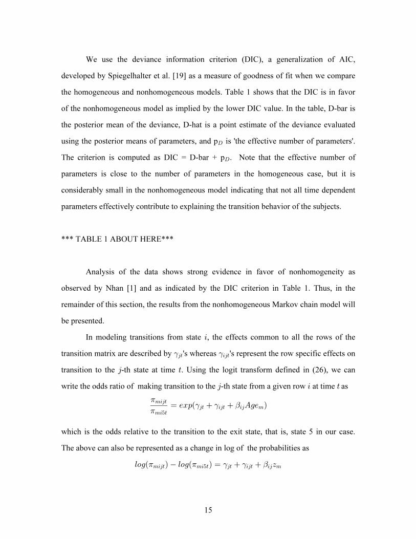
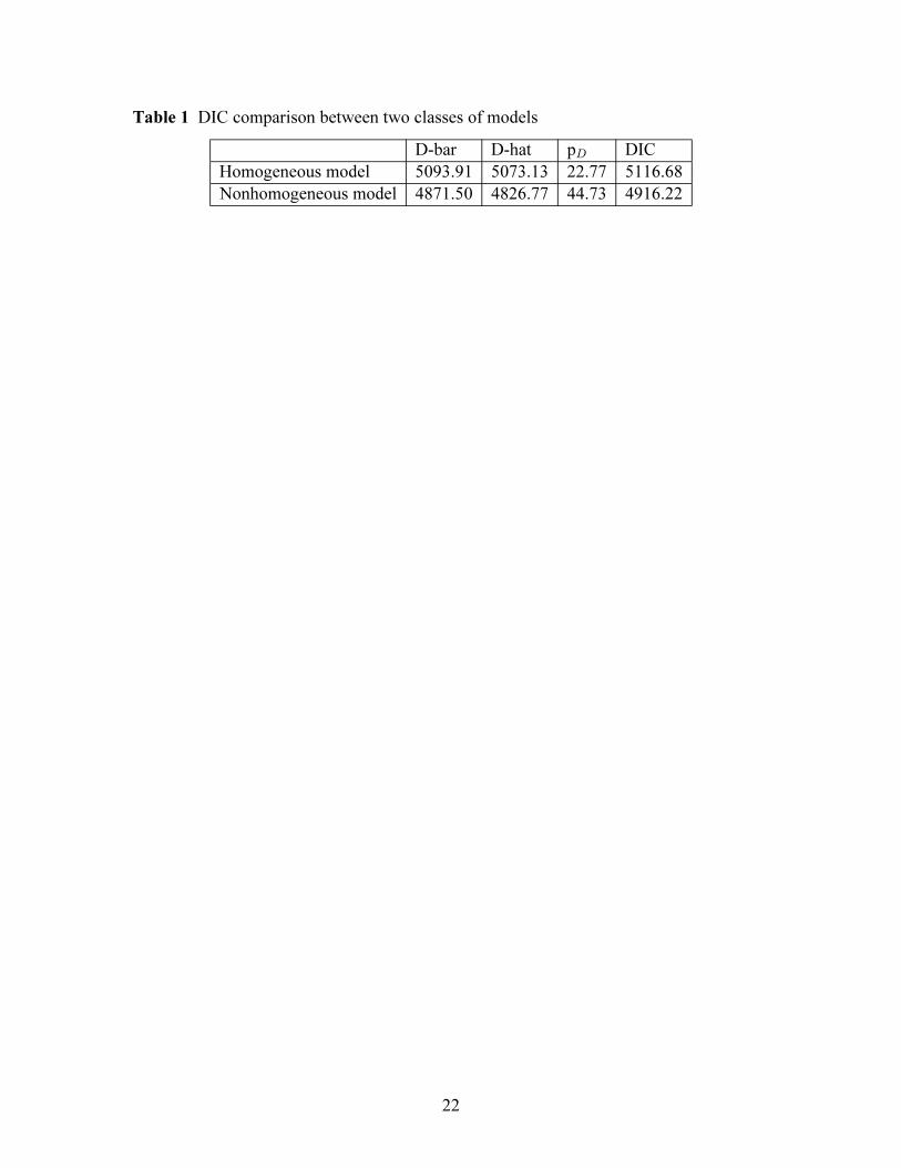
We use the deviance information criterion (DIC), a generalization of AIC,

developed by Spiegelhalter et al. [19] as a measure of goodness of fit when we compare

the homogeneous and nonhomogeneous models. Table 1 shows that the DIC is in favor

of the nonhomogeneous model as implied by the lower DIC value. In the table, D-bar is

the posterior mean of the deviance, D-hat is a point estimate of the deviance evaluated

using the posterior means of parameters, and p is 'the effective number of parameters'.H

The criterion is computed as DIC = D-bar + p . Note that the effective number ofH

parameters is close to the number of parameters in the homogeneous case, but it is

considerably small in the nonhomogeneous model indicating that not all time dependent

parameters effectively contribute to explaining the transition behavior of the subjects.

*** TABLE 1 ABOUT HERE***

Analysis of the data shows strong evidence in favor of nonhomogeneity as

observed by Nhan [1] and as indicated by the DIC criterion in Table 1. Thus, in the

remainder of this section, the results from the nonhomogeneous Markov chain model will

be presented.

In modeling transitions from state , the effects common to all the rows of the3

transition matrix are described by 's whereas 's represent the row specific effects on# #4> 34>

transition to the -th state at time . Using the logit transform defined in (26), we can4 >

write the odds ratio of making transition to the -th state from a given row at time as4 3 >

1

1# # "

734>

73&>4> 34> 34 7œ /B:Ð E1/ Ñ

which is the odds relative to the transition to the exit state, that is, state 5 in our case.

The above can also be represented as a change in log of the probabilities as

691Ð Ñ 691Ð Ñ œ D1 1 # # "734> 73&> 4> 34> 34 7

16

and the component can be interpreted as the expected change in logÐ Ñ# #4> 34>

probabilities what is not described by the covariate.

***TABLE 2 ABOUT HERE***

In Table 2, we present the posterior means and standard deviations of Ð Ñ# #4> "4>

for transitions from state 1. Each posterior distribution represents the values of log odds

with respect to the state 5. We note that as we move from right to the left in a given row

of the table, that is, when we move to better states, the mean of the posterior distribution

decreases. This implies that when we control the age effect, as we move to better states,

the log probability difference between that state and the exit state, that is, state 5,

becomes smaller. Furthermore, this also implies that for transitions from state 1, when we

control the age effect, log odds in favor of staying in state 1 is higher than that of moving

to a higher state. At time 4, for example, the subjects are most likely to remain at the

same state (that is, at state 1), but they are more likely to exit than move to state 4 as

reflected by the negative log odds term. Similar insights can be obtained from posterior

summaries associated with transitions from other rows.

Figure 1 shows how 's for differ over a range of time periods,1#4> 4 œ "ßá ß &

> œ "ßá ß (, for age group 10. From state 2, the transition probabilities to state 3 or 4

slightly increase with time, but transition probabilities to state 1 or 2 decrease with time,

implying that the subjects are more likely to make progress in the treatment program. The

likelihood of discharge rapidly increases with time, and this implies that as time passes

the subjects will exit the program either because they get better or because they do not

show much improvement.

*** FIGURE 1 ABOUT HERE***

17

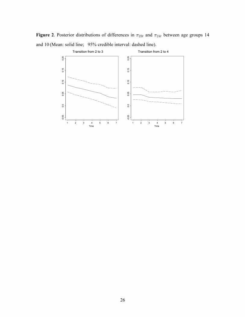
From the analysis, it appears that older children are more likely to make an

improvement than younger children. To assess the effect of age on making improvement

over time, we can compare two age groups, say, 14 and 10. We can examine posterior

probabilities of the quantity

H œ Ö lE1/ œ "%× Ö lE1/ œ "!×" " 34> 34>4 0 1 1 ,

for , that is, we can infer differences in transition probabilities (for improvement)3 4

between the two age groups. Figure 2 shows the mean and 95% credible interval of

posterior distribution of obtained for and . We note that while theH" " #$> #%>4 0 1 1

probability differences are positive and therefore implying more likely improvement for

older children, the differences decrease with time. Furthermore, differences for seem1#$>

to decrease more rapidly than for .1#%>

***FIGURE 2 ABOUT HERE***

In evaluating a treatment program, it is of interest to infer how likely to be

discharged from a given state as well as to infer the reason of these disharges. In other

words, given that a patient is at state at time , we are interested in assessing how3 > "

likely it is for this patient to be discharged at time . Note that this is helpful to be able to>

infer whether patients are discharged because they have responded positively to the

treatment program. The posterior distributions of exit probabilities from each state are

illustrated in Figure 3 for time periods The distributions are presented for> œ "ßá ß (Þ

subjects in the age group of 10. We note in each frame of Figure 3 that the exit

probability increases with time regardless of the prior state. The exit probabilities do not

seem to differ much from one state to the other upto period . After period 4,> œ $ > œ

increase in exit probability seems to be accelerated from states 1 and 4. This implies that

as time passes patients will exit the program either because they get better or because

18

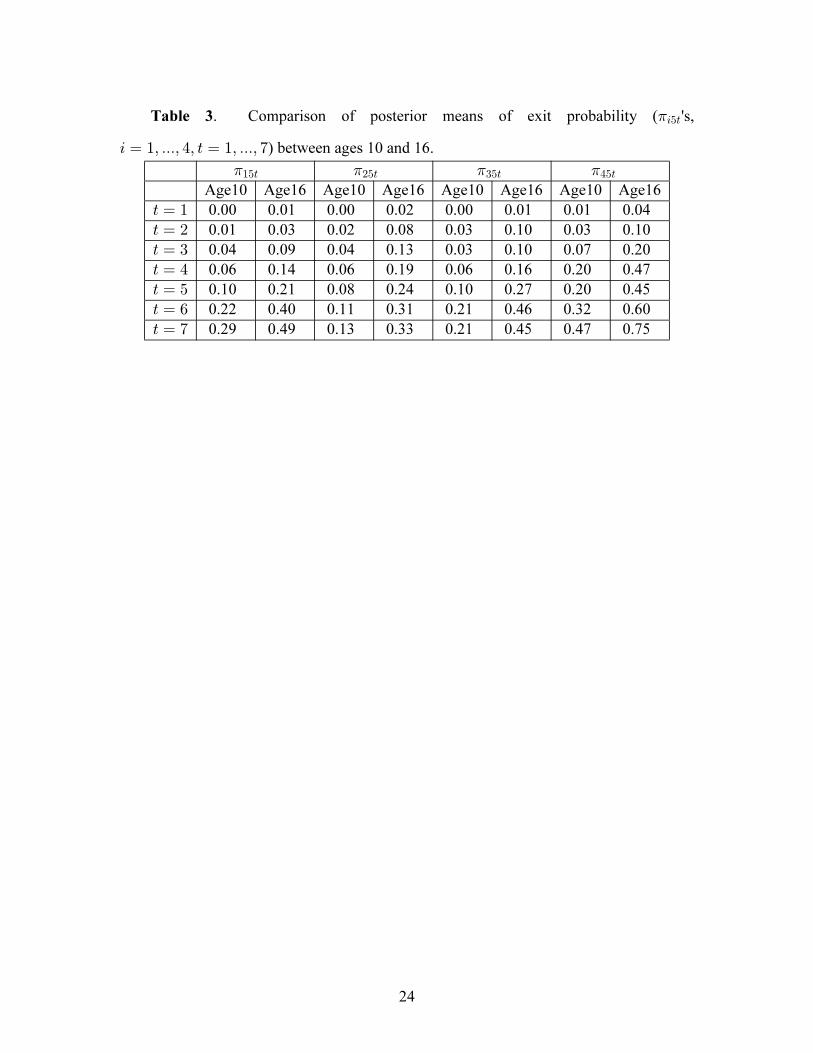
they do not show much improvement. This can also be seen from Table 3 by comparing

the exit probabilities from different states over time. While the overall exit behavior is

similar for other age groups, older patients (age 16) show overall higher exit probabilities

and increasing rates of exit over time than younger patients (age 10) as compared in

Table 3.

***FIGURE 3 ABOUT HERE***

***TABLE 3 ABOUT HERE***

5. Conclusions

In this paper, we presented Bayesian methods for modeling and analyses of

nonhomogeneous Markov chains, and developed inference procedures to be able to

address issues encountered in the analyses of data from psychiatric treatment programs.

As posterior distributions of parameters of interest could not be obtained in analytically

tractable forms, we used simulation (MCMC) based approaches in developing inferences

for the models. The proposed models were implemented using real data from a

psychiatric treatment program and various type of insights that can be obtained from the

Bayesian analysis were illustrated.

The application of the methodology developed in the present study is not limited

to psychiatry and can be extended to other application areas in engineering and sciences.

19

APPENDIX A

Log concavity of :Ð l ß Ñ@ @3 3WÐÑ

The log of (19) can be written as proportional to

" "Š ‹ ‘7ß>ß4

734> 7> 7>4 4 ; ; ; ;4œ"

N

B 691 /B:Ð Ñ J J) ) ) . ) .3 3 3 3 3 3"

#Ð Ñ Ð Ñß"

;œ"

Uw["

;

where the expression J7> 4 4) )3 3 is linear in , and thus the second derivative will be zero.

The last term consists of a negative of a quadratic form which is concave. We next

consider the second term in the bracket in the term. First derivative of the log term,

691 /B:Ð Ñ!4œ"

N

7> 4J )3 is given by

/B:Ð Ñ

/B:Ð Ñ

J

J

7> 4

7> 4

)

)

3

3!4œ"

N

which is defined as in (5), and derivative of this quantity, is1734

/B:Ð Ñ /B:Ð Ñ

/B:Ð Ñ /B:Ð Ñ

" J J

J J

7> 7>4 4

7> 7>4 4

) )

) )

3 3

3 3! !Œ 4œ" 4œ"

N N.

which is always positive and thus implies .the log concavity of (19) in @3

20

REFERENCES

1. Nhan N. . Technical Report. GraydonEffects and outcome of residential treatment

Manor Research Department, VA, 1999.

2. Meredith J. Program evaluation in a hospital for mentally retarded persons. American

Journal of Mental Deficiency 1974; 78:471-481.

3. Cox DR. Statistical analysis of time series: Some recent developments. Scandinavian

Journal of Statistics 1981; 8:93-115.

4. Erkanli A, Soyer R, Angold A. Bayesian analyses of longitudinal binary data using

Markov regression models of unknown order. 2001; 20:755-Statistics in Medicine

770.

5. Cargnoni C, Müller P, West M. Bayesian forecasting of multinomial time series

through conditionally Gaussian dynamic models. Journal of the American Statistical

Association 1997; 92:640-647.

6. Harrison P, Stevens C. Bayesian forecasting (with discussion). Journal of the Royal

Statistical Society, Ser. B 1976; 38:205-247.

7. West M, Harrison J, Migon H. Dynamic generalized linear models and Bayesian

forecasting. 1985; 80:73-97.Journal of the American Statistical Association

8. Anderson TW, Goodman LA. Statistical inference about Markov chains. Annals of

Mathematical Statistics 1957; 28:89-110.

9. Lee TC, Judge GG, Zellner A. Estimating the Parameters of the Markov Probability

Model from Aggregate Time Series Data. North-Holland and Pub. Co.: Amsterdam,

1970.

10. Meshkani M. Empirical Bayes estimation of transition probabilities for Markov

chains. Ph.D. Dissertation. Florida State University, 1978.

11. Morris CN. Parametric empirical Bayes inference: Theory and applications. Journal

of American Statistical Association 1983; 78:47-65.

21

12. Muenz L, Rubinstein L. Markov models for covariate dependence of binary

sequences. 1985; 41:91-101.Biometrics

13. Zeger S, Qaqish B. Markov regression models for time series: A quasi-likelihood

approach. 1988; 44:1019-1031.Biometrics

14. Diggle P, Liang K, Zeger S. . Oxford ScienceAnalysis of Longitudinal Data

Publications: Oxford, 1994.

15. Grunwald G, Raftery A, Guttorp P. Time series for continuous proportions. Journal

of the Royal Statistical Society, Ser. B 1993; 55:103-116.

16. Gilks W, Wild P. Adaptive rejection sampling for Gibbs sampling. Journal of the

Royal Statistical Society, Ser. B 1992; 41:337-348.

17. Spiegelhalter D, Thomas A, Best N, Gilks W. Bayesian Inference Using Gibbs

Sampling Manual (version ii). MRC Biostatistics Unit, Cambridge University, 1996.

18. Brooks SP, Gelman A. Alternative methods for monitoring convergence of iterative

simulations. 1998; 7:434-455.Journal of Computational and Graphical Statistics

19. Spiegelhalter D, Best N, Carlin BR,van der Linde A. Bayesian measures of model

complexity and fit. 2002; 64:583-616.Journal of the Royal Statistical Society, Ser. B

22

Table 1 DIC comparison between two classes of models

D-bar D-hat p DIC

Homogeneous model 5093.91 5073.13 22.77 5116.68

Nonhomogeneous model 4871.50 4826.77 44.73 4916.22

H

23

Table 2. Posterior means and standard deviations (SD) of fixed effects for transitions

from State 1.

Mean SD Mean SD Mean SD Mean SD

# # # # # # # #"> ""> #> "#> $> "$> %> "%>

> œ " (Þ&$ !Þ*" 'Þ"( !Þ)% %Þ## !Þ)% #Þ#% "Þ"%> œ # &Þ'! !Þ(" %Þ%' !Þ&* #Þ&% !Þ%& !Þ'! !Þ&"> œ $ %Þ'" !Þ'# $Þ&" !Þ'# "Þ#) !Þ&" "Þ!' !Þ&*> œ % $Þ*) !Þ&) #Þ*# !Þ&$ !Þ(* !Þ&' "Þ&!

!Þ'(> œ & $Þ&" !Þ&" #Þ%' !Þ%) !Þ$! !Þ&% #Þ!* !Þ()> œ ' #Þ&% !Þ'! "Þ&& !Þ&* !Þ'$ !Þ&$ $Þ"% !Þ)"> œ ( #Þ") !Þ&% "Þ"* !Þ&* "Þ!! !Þ&

& $Þ&% !Þ)#

24

. Comparison of posterior means of exit probability ( 's,Table 3 13&>

3 œ "ß ÞÞÞß %ß > œ "ß ÞÞÞß () between ages 10 and 16.

Age10 Age16 Age10 Age16 Age10 Age16 Age10 Age16

0.00 0.01 0.00 0.02 0.00 0.01 0.01 0.04

0.01 0.03 0.0

1 1 1 1"&> #&> $&> %&>

> œ "> œ # 2 0.08 0.03 0.10 0.03 0.10

0.04 0.09 0.04 0.13 0.03 0.10 0.07 0.20

0.06 0.14 0.06 0.19 0.06 0.16 0.20 0.47

0.10 0.21

> œ $> œ %> œ & 0.08 0.24 0.10 0.27 0.20 0.45

0.22 0.40 0.11 0.31 0.21 0.46 0.32 0.60

0.29 0.49 0.13 0.33 0.21 0.45 0.47 0.75

> œ '> œ (

25

Figure 1. Posterior transition probabilities from state 2 at different time points for age 10

(Mean: solid line; 95% credible interval: dashed line)

Transition from 2 to 1

Time

1 2 3 4 5 6 7

0.0

0.1

0.2

0.3

0.4

0.5

Transition from 2 to 2

Time

1 2 3 4 5 6 7

0.0

0.1

0.2

0.3

0.4

0.5

Transition from 2 to 3

Time

1 2 3 4 5 6 7

0.0

0.1

0.2

0.3

0.4

0.5

Transition from 2 to 4

Time

1 2 3 4 5 6 7

0.0

0.1

0.2

0.3

0.4

0.5

Transition from 2 to Exit

Time

1 2 3 4 5 6 7

0.0

0.1

0.2

0.3

0.4

0.5

26

Figure 2. Posterior distributions of differences in and between age groups 141 1#$> #%>

and 10 (Mean: solid line; 95% credible interval: dashed line).

Transition from 2 to 3

Time

1 2 3 4 5 6 7

-0.05

0.0

0.05

0.10

0.15

0.20

Transition from 2 to 4

Time

1 2 3 4 5 6 7

-0.05

0.0

0.05

0.10

0.15

0.20

27

Figure 3. Posterior distributions of exit probability ( 's) from each state at :13&> > œ "ß ÞÞÞß (

Age=10 (Mean: solid line; 95% credible interval: dashed line)

Exit from state 1

Time

1 2 3 4 5 6 7

0.0

0.2

0.4

0.6

0.8

Exit from state 2

Time

1 2 3 4 5 6 7

0.0

0.2

0.4

0.6

0.8

Exit from state 3

Time

1 2 3 4 5 6 7

0.0

0.2

0.4

0.6

0.8

Exit from state 4

Time

1 2 3 4 5 6 7

0.0

0.2

0.4

0.6

0.8