Basics of Image Processing

PRESENTED BY

R.SARAVANAN, R ES EA R C H S C HOLA R ,

D E PA RT M E N T O F I N F O R M AT I O N T E C H N O L O G Y,

M A D R A S I N S T I T U T E O F T E C H N O L O G Y, A N N A U N I V E R S I T Y.

Basics of Image

Processing

Topics

Image Processing Basics

MATLAB Basics and IPT

Image Sensing and Acquisition

Arithmetic and Logic Operation

Geometric Operations

Gray-Level Transformation

Histogram Processing

Neighborhood Processing

Image Processing Basics

Digital Image representation

- A Digital Image – whether it was obtained as a result of Sampling

and Quantization of an analog image or created already in digital form-

can be represented as a 2D matrix of real numbers.

- The value of the 2D function f(x, y) at any given pixel of

coordinates (x0, y0), denoted by f(x0,y0) is called the intensity or gray

level of the image at the pixel

- Common ranges are as follows:

double data type : 0.0 (black) and 1.0 (white)

uint8(unsigned integer, 8 bit) : 0 (black) and 255(white)

Image Processing Basics

cont.,

Binary Images - Binary images are encoded as a 2D array, typically using 1 bit per

pixel, where a 0 usually means “black” and a 1 means “white”

Image Processing Basics

Gray Level (8-Bit) Images

- Its also called as monochrome images are also encoded as a 2D

array of pixels, usually with 8 bits per pixel, where a pixel value of 0

corresponds to “black”, a pixel value 255 means “white”, and

intermediate values indicate varying shades of gray.

Image Processing Basics

cont.,

Color Images

- Representation of color images is more complex and varied.

two ways of storing color image contents i) RGB representation- in

which each pixel is usually represented by a 24 bit number contain the

amount of R G B components, ii) indexed representation - where a 2D

array contains indices to a color palette (or lookup table-LUT).

- 24 Bit (RGB) Color images, can be represented using three 2D

arrays of same size, one for each color channel, R,G and B. Each array

element contains an 8 bit value, indicates the amount of RGB at the

point in a [0, 255]

Image Processing Basics

cont.,

Color Image

Color image (a) and its R(b), G(c), and B(d) Components

Image Processing Basics

cont.,

Indexed Color Images

- indexed representation, in which a 2D array of the same size as

the image contains pointers to a color map of fixed maximum size

MATLAB Basics

Introduction to MATLAB

- MATLAB (MATrix LABoratory) is a data analysis, prototyping

and visualization tool with built in support for matrices and matrix

operations, excellent graphics capabilities, and a high level

programming language and development environment.

- Working Environment consists of MATLAB Desktop, this

contains Command Window, the Workspace Browser, The Current

Directory Window, The Command History and Figure Windows,

MATLAB Editor used to create and edit the M files and MATLAB help

system includes the Help Browser, Which displays HTML, documents

and contains a number of search and display options.

MATLAB Basics Cont.,

Data Types

- uint8 ---- 8-Bit unsigned integers (1 byte per element)

- uint16---- 16-Bit unsigned integers (2 bytes per element)

- uint32---- 32-Bit unsigned integers (4 bytes per element)

- int8 ----8-Bit signed integers (1 byte per element)

- int16---- 16-Bit signed integers (2 bytes per element)

- int32---- 32-Bit signed integers (4 bytes per element)

- single---- Single-precision floating numbers (4 bytes per element)

- double--- Double-precision floating numbers (8 bytes per element)

- logical ----Values are 0 (false) or 1 (true) (1 byte per element)

- char ----Characters (2 bytes per element)

MATLAB Basics

Cont.,

Standard Array

- Build in standard arrays:

• zeros(m, n) creates an m × n matrix of zeros.

• ones(m, n) creates an m × n matrix of ones.

• true(m, n) creates an m × n matrix of logical ones.

• false(m, n) creates an m × n matrix of logical zeros.

• eye(n) returns an n × n identity matrix.

• magic(m) returns a magic square2 of order m.

• rand(m, n) creates an m × n matrix whose entries are pseudo

random numbers uniformly distributed in the interval [0, 1].

MATLAB Basics

Cont.,

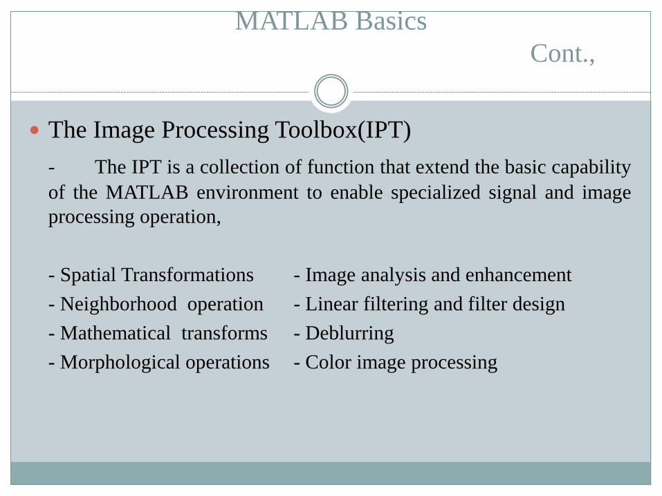
The Image Processing Toolbox(IPT)

- The IPT is a collection of function that extend the basic capability

of the MATLAB environment to enable specialized signal and image

processing operation,

- Spatial Transformations - Image analysis and enhancement

- Neighborhood operation - Linear filtering and filter design

- Mathematical transforms - Deblurring

- Morphological operations - Color image processing

MATLAB Basics

Cont.,

Essential Function and Features

- Displaying Information About an image File

imfinfo (‘filename’) display the information about graphics file

Reading an Image file

- imread function to open and read the contents of all popular

formats.(e.g: TIFF,JPEG,BMP,GIF, and PNG) and this function allows

to read image files of all type, in virtually ant format, located

anywhere.

- dicomread for DICOM(Digital Imaging and Communication in

Medicine) files, nitfread for NITF(National Imagery Transmission

Format) files, and hdrread for HDR (High Dynamic Range) files

MATLAB Basics

Cont.,

Data Classes and Data Conversions - The most common data class for images are

uint8: 1 byte per pixel, in the [0,255] range.

double: 8 bytes per pixel, usually in the [0.0, 1.0] range

logical: 1 byte per pixel, its value as true(White) or false (Black)

- To convert an image to data class and range suitable for image processing.,

MATLAB Basics

Cont.,

Displaying the Contents of an image

- image: Displays an image using the current color map

- imagesc: Scales image data to the full range of the current color map

and display the image.

- imshow: Display an image and contains a number of optimizations

and optional parameters for property settings associated with image

display.

- imtool: Display an image and contains a number of associated tools

that can be used to explore the image content.

Two other IPT functions: impixel returns the red, green and blue color

values of image, imdistline creates the Distance tools that’s measure the

distance between its endpoints.,

Image Acquisition Image Sensors and Optics

- Image sensors: The main goal of an image sensor is to convert EM energy into electrical signals that can be processed, displayed, and interpreted as image.

- Camera Optics: A camera uses a lens to focus part of the scene onto the image sensor. Two of the most important parameters of a lens are its magnifying power and light gathering capacity.

Image Acquisition Cont.,

Image Digitization

- Involves two processes: Sampling (in time or space) and

quantization (in amplitude). These operation may occurs in any

sequence, but usually sampling precedes quantization.

- Sampling involves selecting a finite number of points within an

interval, whereas quantization implies assigning an finite range of

possible amplitude value to each of those points.

- Sampling is the process of measuring the value of a 2D function at

discrete intervals along the x and y dimensions and the quantization

is the process of replacing a continuously varying function with a

discrete set of quantization levels

- In MATLAB, (Re)-Quantizing an image can be accomplished using

grayslice function.

Example of Quantizing in MATLAB: (a)480 x 640 image, 256 gray level: (b-h) image requantized

to 128, 64, 32, 16, 8, 4 and 2 gray levels

ARITHMETIC AND LOGIC OPERATIONS

Arithmetic Operations: Fundamentals

- Performed on a pixel-by-pixel basis, the operation is independently

applied to each pixel in the image. Two 2D array (a) and (b) the

resulting array (c), is obtained by calculating A opn B = C, where

the opn is a binary arithmetic (+,-,*,/) operator. Eg, addition

ARITHMETIC OPERATIONS

Cont.,

Addition

- Addition is used to blend the pixel contents from two images or add

a constant value to pixel value of an image. Adding the contents of

two monochrome images causes their contents to blend. Adding a

constant value (scalar) to an image causes an increase in its overall

brightness, a process sometimes referred to as additive image offset

ARITHMETIC OPERATIONS

Cont.,

Subtraction

- Its often used to detect differences between two images. Such differences

may be due to several factors, such as artificial addition to or removal of

relevant contents from the image, relative object motion between two

frames of a video sequence, and many others. Subtracting a constant value

from an image causes a decrease in its overall brightness, a process

sometimes called as a subtractive image offset. (Negative image also possible)

ARITHMETIC OPERATIONS

Cont., Multiplication and Division

- Multiplication and division by a scalar are often used to perform brightness

adjustments on an image. This process sometimes called as a multiplicative image

scaling masks each pixel value brighter or darker by multiplying its original value

by a scalar factor: if the value of the scalar multiplication factor is greater than one,

the result is a brighter image; if it is greater than zero and less than one, it results in

darker image. Multiplication and division by a constant: (a) original image (X);

(b) multiplication result (X × 0.7); (c) division result (X/0.7).

LOGIC OPERATIONS

Logic Operations: Fundamentals

- Logic operations are performed in a bit wise fashion on the binary

contents of each pixel value. The AND, XOR and OR operators required a

two or more arguments, the NOT operator requires only one argument. They

are used to in masking operations, and extract the ROI.

LOGIC OPERATIONS

Logic Operations: In MATLAB

- XOR operation is often used to highlight a difference between the

two images and NOT operation extracts the binary complement of

each pixel value, which is equal to applying the negative effect. In

MATLAB, bitand, bitor, bitxor and bitcmp are in build functions.

AND operation applied to monochrome images: (a) X; (b) Y; (c) X AND

LOGIC OPERATIONS

The OR operation applied to monochrome images: (a) X; (b) Y; (c) X OR Y.

The XOR operation applied to monochrome images: (a) X; (b) Y; (c) X XOR Y.

GEOMETRIC OPERATIONS

Introduction

- Geometric operations modify the geometry of an image by repositioning

pixels in a constrained way. In other words, rather than changing the pixel

values of an image, they modify the spatial relationships between groups of

pixels representing features or objects of interest within the image

- Geometric operation goals :

* Correcting geometric distortions introduced during the image

acquisition process.

* Creating special effects on existing images, such as twirling,

bulging, or squeezing a picture of someone’s face.

- Geometric operation Components:

* Mapping Function (Specified using a set of spatial transformation)

* Interpolation Methods (Compute the new pixel value)

GEOMETRIC OPERATIONS

Using MATLAB,

- Zooming, Shrinking and Resizing

- Translation

- Rotation

- Cropping

- Flipping

Other Geometric Operations,

- Warping

- Nonlinear Image Transformation

- Twirling

- Ripping

- Morphing

- Seam Carving

GRAY LEVEL TRANSFORMATIONS

Introduction

- To improve the subjective quality of an image for human viewing.

- To modify the image in such a way as to make it more suitable for

further analysis and automatic extraction of its contents.

Gray-Level (Point) Transformations

The point operations are also referred to as gray-level transformation

or spatial transformations. They can be expressed as

g(x, y) = T [f(x, y)]

Where g(x, y) is the processed image, f(x, y) is the original image,

and T is an operator on f(x, y)

GRAY LEVEL TRANSFORMATIONS

Examples of Point Transformations

- Contrast Manipulation (contrast Stretching, gray level stretching)

- In mat lab, imcontrast

- Negative (contrast reverse)

- In mat lab, imcomplement

- Power Law (Gamma) Transformations function is s = c . rˠ where

the r is the original pixel value, s is the resulting constant pixel

value, c is a scaling and gamma is the .positive value

- In mat lab, syntax g = imadjust (f, [],[],gamma);

- Log Transformations and its inverse are nonlinear transformations

used, when we want to compress or expand the dynamic range of

pixels values in an image. s = c . log(1 + r) where r is the original, s

is the resulting value, and c is a constant.

HISTOGRAM PROCESSING

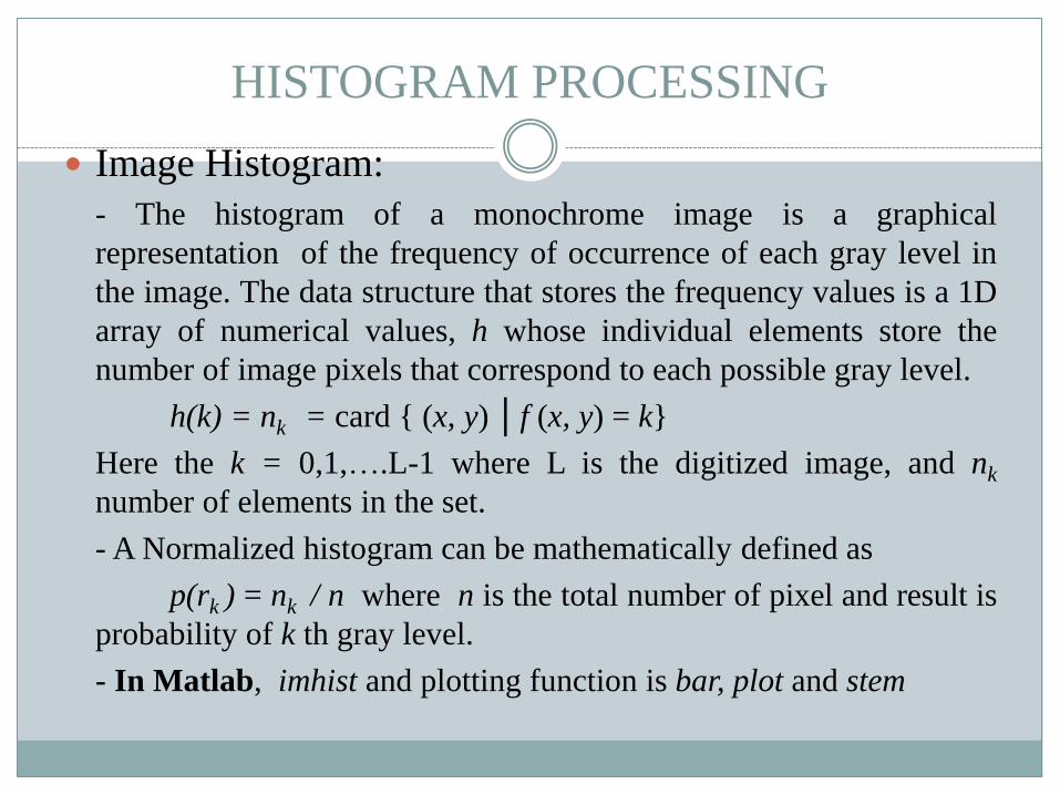
Image Histogram:

- The histogram of a monochrome image is a graphical

representation of the frequency of occurrence of each gray level in

the image. The data structure that stores the frequency values is a 1D

array of numerical values, h whose individual elements store the

number of image pixels that correspond to each possible gray level.

h(k) = nk = card { (x, y) │f (x, y) = k}

Here the k = 0,1,….L-1 where L is the digitized image, and nk

number of elements in the set.

- A Normalized histogram can be mathematically defined as

p(rk ) = nk / n where n is the total number of pixel and result is

probability of k th gray level.

- In Matlab, imhist and plotting function is bar, plot and stem

HISTOGRAM EQUALIZATION

Histogram equalization is a technique by which the gray level

distribution of an image is changed in such a way as to obtain a

uniform resulting histogram, in which the percentage of pixel of

every gray level same.

In Matlab, build in function histeq to perform a histogram

equalization, the syntax is a histeq(I, n) where n is the number

desired gray levels in the output image (default n is 64).

Other Histogram Techniques: which histogram can be

processed to achieved a specific goal, such as a brightness increase

or decrease or contrast improvement.

- Histogram Sliding technique consists of simply adding or

subtracting a constant brightness value to all pixel in the image. The

overall brightness is calculated by average. In MATLAB, The imadd

and imsubtract used for histogram sliding

HISTOGRAM EQUALIZATION

- Histogram Stretching technique also known as input cropping –

consists of a linear transformation that expands (stretches) part of the

original histogram so that its nonzero intensity range [rmin ,rmax ]

occupies the full dynamic gray scale, [0, L-1].

- Histogram Shrinking technique also known as output cropping –

modifies the original histogram in such a way as to compress its

dynamic grayscale range, [rmin ,rmax ], into narrower gray scale,

between smin and smax .

- In Matlab, IPT built in function to perform histogram stretching

and shrinking using imadjust

NEIGHBORHOOD PROCESSING

Steps of neighborhood processing operation. (both linear or nonlinear)

* Define a reference point in the input image, f(x0, y0)

* Perform an operation that involves only pixel within a neighborhood

around the reference point in the input image.

* Apply the result of that operation to the pixel of some coordinates in

the output image, g(x0, y0).

* Repeat the process for the every pixel in the input image.

The neighborhood processing belongs to one of these two categories:

* Linear Filters (Mean Filter)

* Nonlinear filters (Median Filter)

NEIGHBORHOOD PROCESSING

Convolution and Correlation in MATLAB

* conv2: It computes the 2D convolution between two matrices.

full: Returns the full 2D convolution

same: Returns the central part of the convolution of the same size as A.

valid: Returns only the convolution that are computed without the zero

padded edges.

* filter2: It rotates the convolution mask 180degree in each direction to

create a convolution kernel and call the convolution function.

The convolution and correlation so far has overlooked the need to deal

with image borders, the part of the mask falls outside in the image

border.

NEIGHBORHOOD PROCESSING

Image Smoothing (Low Pass Filter)

- Low pass filter those spatial filters whose effect on the output image is equivalent to attenuating high frequency components.

- In Matlab, Linear filters are implemented by two basic functions: imfilter and optionally fspecial.

g = imfilter (f, h, mode, boundary_options, size_options);

g is the input image, h is the filter mask, mode can be in convolution ‘conv’ or correlation ‘corr’, boundary_options are refer the algorithm based on boundary. size_options are two options are ‘same’ or ‘full’, and g is the output image.

NEIGHBORHOOD PROCESSING

In fspecial is an function created a 2D image filter, syntax is

h= fspecial (type, parameters) where h is the filter mask

type is one of the following,

’average’: Averaging filter

’disk’: Circular averaging filter

’gaussian’: Gaussian low-pass filter

’laplacian’: 2D Laplacian operator

’log’: Laplacian of Gaussian (LoG) filter

’motion’: Approximates the linear motion of a camera

’prewitt’ and ’sobel’: horizontal edge-emphasizing filters

’unsharp’: unsharp contrast enhancement filter

parameter is optional that vary depending on the type of the filter.

NEIGHBORHOOD PROCESSING

Image Sharpening (High Pass Filter)

- High Pass filter those spatial filters whose effect on an image is

equivalent to preserving or emphasizing its high-frequency components

(i.e., fine details, points, lines and edges) that is, to highlight transitions

in intensity within the image.

- Linear HPFs can be implemented using 2D convolution masks with

positive and negative coefficients, which correspond to a digital

approximation of the laplacian a simple, isotropic second order

derivative that is capable of responding to intensity transitions in any

direction.

THANK YOU