Basic Queueing Theory Dr. János Sztrik University of Debrecen, Faculty of Informatics

Welcome message from author
This document is posted to help you gain knowledge. Please leave a comment to let me know what you think about it! Share it to your friends and learn new things together.
Transcript
Basic Queueing Theory
Dr. János Sztrik
University of Debrecen, Faculty of Informatics

Reviewers:
Dr. József BíróDoctor of the Hungarian Academy of Sciences, Full Professor
Budapest University of Technology and Economics
Dr. Zalán HeszbergerPhD, Associate Professor
Budapest University of Technology and Economics
2

This book is dedicated to my wife without whom thiswork could have been finished much earlier.
• If anything can go wrong, it will.
• If you change queues, the one you have left will start to move faster than the oneyou are in now.
• Your queue always goes the slowest.
• Whatever queue you join, no matter how short it looks, it will always take thelongest for you to get served.
( Murphy’ Laws on reliability and queueing )
3

4

Contents
Preface 7
I Basic Queueing Theory 9
1 Fundamental Concepts of Queueing Theory 111.1 Performance Measures of Queueing Systems . . . . . . . . . . . . . . . . 121.2 Kendall’s Notation . . . . . . . . . . . . . . . . . . . . . . . . . . . . . . 141.3 Basic Relations for Birth-Death Processes . . . . . . . . . . . . . . . . . 151.4 Queueing Softwares . . . . . . . . . . . . . . . . . . . . . . . . . . . . . . 16
2 Infinite-Source Queueing Systems 172.1 The M/M/1 Queue . . . . . . . . . . . . . . . . . . . . . . . . . . . . . . 172.2 The M/M/1 Queue with Balking Customers . . . . . . . . . . . . . . . . 252.3 Priority M/M/1 Queues . . . . . . . . . . . . . . . . . . . . . . . . . . . 302.4 The M/M/1/K Queue, Systems with Finite Capacity . . . . . . . . . . . 322.5 The M/M/∞ Queue . . . . . . . . . . . . . . . . . . . . . . . . . . . . . 372.6 The M/M/n/n Queue, Erlang-Loss System . . . . . . . . . . . . . . . . 382.7 The M/M/n Queue . . . . . . . . . . . . . . . . . . . . . . . . . . . . . . 442.8 The M/M/c/K Queue - Multiserver, Finite-Capacity Systems . . . . . . 552.9 The M/G/1 Queue . . . . . . . . . . . . . . . . . . . . . . . . . . . . . . 57
3 Finite-Source Systems 693.1 The M/M/r/r/n Queue, Engset-Loss System . . . . . . . . . . . . . . . 693.2 The M/M/1/n/n Queue . . . . . . . . . . . . . . . . . . . . . . . . . . . 733.3 Heterogeneous Queues . . . . . . . . . . . . . . . . . . . . . . . . . . . . 88
3.3.1 The ~M/ ~M/1/n/n/PS Queue . . . . . . . . . . . . . . . . . . . . 893.4 The M/M/r/n/n Queue . . . . . . . . . . . . . . . . . . . . . . . . . . . 923.5 The M/M/r/K/n Queue . . . . . . . . . . . . . . . . . . . . . . . . . . . 1043.6 The M/G/1/n/n/PS Queue . . . . . . . . . . . . . . . . . . . . . . . . . 1063.7 The ~G/M/r/n/n/FIFO Queue . . . . . . . . . . . . . . . . . . . . . . . 109
II Exercises 117
4 Infinite-Source Systems 119
5
5 Finite-Source Systems 137
III Queueing Theory Formulas 141
6 Relationships 1436.1 Notations and Definitions . . . . . . . . . . . . . . . . . . . . . . . . . . 1436.2 Relationships between random variables . . . . . . . . . . . . . . . . . . 145
7 Basic Queueing Theory Formulas 1477.1 M/M/1 Formulas . . . . . . . . . . . . . . . . . . . . . . . . . . . . . . . 1477.2 M/M/1/K Formulas . . . . . . . . . . . . . . . . . . . . . . . . . . . . . 1497.3 M/M/c Formulas . . . . . . . . . . . . . . . . . . . . . . . . . . . . . . . 1507.4 M/M/2 Formulas . . . . . . . . . . . . . . . . . . . . . . . . . . . . . . . 1527.5 M/M/c/c Formulas . . . . . . . . . . . . . . . . . . . . . . . . . . . . . . 1547.6 M/M/c/K Formulas . . . . . . . . . . . . . . . . . . . . . . . . . . . . . 1557.7 M/M/∞ Formulas . . . . . . . . . . . . . . . . . . . . . . . . . . . . . . 1577.8 M/M/1/K/K Formulas . . . . . . . . . . . . . . . . . . . . . . . . . . . . 1587.9 M/G/1/K/K Formulas . . . . . . . . . . . . . . . . . . . . . . . . . . . . 1607.10 M/M/c/K/K Formulas . . . . . . . . . . . . . . . . . . . . . . . . . . . . 1617.11 D/D/c/K/K Formulas . . . . . . . . . . . . . . . . . . . . . . . . . . . . 1637.12 M/G/1 Formulas . . . . . . . . . . . . . . . . . . . . . . . . . . . . . . . 1647.13 GI/M/1 Formulas . . . . . . . . . . . . . . . . . . . . . . . . . . . . . . . 1737.14 GI/M/c Formulas . . . . . . . . . . . . . . . . . . . . . . . . . . . . . . . 1757.15 M/G/1 Priority queueing system . . . . . . . . . . . . . . . . . . . . . . 1777.16 M/G/c Processor Sharing system . . . . . . . . . . . . . . . . . . . . . . 1857.17 M/M/c Priority system . . . . . . . . . . . . . . . . . . . . . . . . . . . . 186
Bibliography 193
6

Preface
Modern information technologies require innovations that are based on modeling, ana-lyzing, designing and finally implementing new systems. The whole developing processassumes a well-organized team work of experts including engineers, computer scientists,mathematicians, physicist just to mention some of them. Modern infocommunicationnetworks are one of the most complex systems where the reliability and efficiency of thecomponents play a very important role. For the better understanding of the dynamicbehavior of the involved processes one have to deal with constructions of mathematicalmodels which describe the stochastic service of randomly arriving requests. QueueingTheory is one of the most commonly used mathematical tool for the performance evalu-ation of such systems.
The aim of the book is to present the basic methods, approaches in a Markovianlevel for the analysis of not too complicated systems. The main purpose is to understandhow models could be constructed and how to analyze them. It is assumed the reader hasbeen exposed to a first course in probability theory, however in the text I give a refresherand state the most important principles I need later on. My intention is to show what isbehind the formulas and how we can derive formulas. It is also essential to know whichkind of questions are reasonable and then how to answer them.
My experience and advice are that if it is possible solve the same problem in differentways and compare the results. Sometimes very nice closed-form, analytic solutions areobtained but the main problem is that we cannot compute them for higher values of theinvolved variables. In this case the algorithmic or asymptotic approaches could be veryuseful. My intention is to find the balance between the mathematical and practitionerneeds. I feel that a satisfactory middle ground has been established for understandingand applying these tools to practical systems. I hope that after understanding this bookthe reader will be able to create his owns formulas if needed.
It should be underlined that most of the models are based on the assumption that theinvolved random variables are exponentially distributed and independent of each other.We must confess that this assumption is artificial since in practice the exponential distri-bution is not so frequent. However, the mathematical models based on the memorylessproperty of the exponential distribution greatly simplifies the solution methods resultingin computable formulas. By using these relatively simple formulas one can easily foreseethe effect of a given parameter on the performance measure and hence the trends can beforecast. Clearly, instead of the exponential distribution one can use other distributionsbut in that case the mathematical models will be much more complicated. The analytic
7
results can help us in validating the results obtained by stochastic simulation. This ap-proach is quite general when analytic expressions cannot be expected. In this case notonly the model construction but also the statistical analysis of the output is important.
The primary purpose of the book is to show how to create simple models for practicalproblems that is why the general theory of stochastic processes is omitted. It uses onlythe most important concepts and sometimes states theorem without proofs, but each timethe related references are cited.
I must confess that the style of the following books greatly influenced me, even ifthey are in different level and more comprehensive than this material: Allen [2], Jain [41],Kleinrock [48], Kobayashi and Mark [51], Stewart [74], Tijms [91], Trivedi [94].
This book is intended not only for students of computer science, engineering, operationresearch, mathematics but also those who study at business, management and planningdepartments, too. It covers more than one semester and has been tested by graduatestudents at Debrecen University over the years. It gives a very detailed analysis of theinvolved queueing systems by giving density function, distribution function, generatingfunction, Laplace-transform, respectively. Furthermore, Java-applets are provided to cal-culate the main performance measures immediately by using the pdf version of the book ina WWW environment. Of course these applets can be run if one reads the printed version.
I have attempted to provide examples for the better understanding and a collectionof exercises with detailed solution helps the reader in deepening her/his knowledge. Iam convinced that the book covers the basic topics in stochastic modeling of practicalproblems and it supports students in all over the world.
I am indebted to Professors József Bíró and Zalán Heszberger for their review, com-ments and suggestions which greatly improved the quality of the book. I am also verygrateful to Tamás Török, Zoltán Nagy and Ferenc Veres for their help in editing. .
All comments and suggestions are welcome at:
[email protected]://irh.inf.unideb.hu/user/jsztrik
Debrecen, 2012.
János Sztrik
8
Part I
Basic Queueing Theory
9


Chapter 1
Fundamental Concepts of QueueingTheory
Queueing theory deals with one of the most unpleasant experiences of life, waiting. Queue-ing is quite common in many fields, for example, in telephone exchange, in a supermarket,at a petrol station, at computer systems, etc. I have mentioned the telephone exchangefirst because the first problems of queueing theory was raised by calls and Erlang wasthe first who treated congestion problems in the beginning of 20th century, see Erlang[21, 22].
His works inspired engineers, mathematicians to deal with queueing problems usingprobabilistic methods. Queueing theory became a field of applied probability and many ofits results have been used in operations research, computer science, telecommunication,traffic engineering, reliability theory, just to mention some. It should be emphasized thatis a living branch of science where the experts publish a lot of papers and books. Theeasiest way is to verify this statement one should use the Google Scholar for queueing re-lated items. A Queueing Theory Homepage has been created where readers are informedabout relevant sources, for example books, softwares, conferences, journals, etc. I highlyrecommend to visit it at
http://web2.uwindsor.ca/math/hlynka/queue.html
There is only a few books and lectures notes published in Hungarian language, I wouldmention the work of Györfi and Páli [33], Jereb and Telek [43], Kleinrock [48], Lakatosand Szeidl , Telek [55] and Sztrik [84, 83, 82, 81]. However, it should be noted that theHungarian engineers and mathematicians have effectively contributed to the research andapplications. First of all we have to mention Lajos Takács who wrote his pioneer and fa-mous book about queueing theory [88]. Other researchers are J. Tomkó, M. Arató, L.Györfi, A. Benczúr, L. Lakatos, L. Szeidl, L. Jereb, M. Telek, J. Bíró, T. Do, and J.Sztrik. The Library of Faculty of Informatics, University of Debrecen, Hungary offer avaluable collection of queueing and performance modeling related books in English, andRussian, too. Please visit:
http://irh.inf.unideb.hu/user/jsztrik/education/05/3f.html
I may draw your attention to the books of Takagi [85, 86, 87] where a rich collection ofreferences is provided.
11
1.1 Performance Measures of Queueing SystemsTo characterize a queueing system we have to identify the probabilistic properties of theincoming flow of requests, service times and service disciplines. The arrival process canbe characterized by the distribution of the interarrival times of the customers, denotedby A(t), that is
A(t) = P ( interarrival time < t).
In queueing theory these interarrival times are usually assumed to be independent andidentically distributed random variables. The other random variable is the service time,sometimes it is called service request, work. Its distribution function is denoted by B(x),that is
B(x) = P ( service time < x).
The service times, and interarrival times are commonly supposed to be independentrandom variables.
The structure of service and service discipline tell us the number of servers,the capacity of the system, that is the maximum number of customers staying in thesystem including the ones being under service. The service discipline determines therule according to the next customer is selected. The most commonly used laws are
• FIFO - First In First Out: who comes earlier leaves earlier
• LIFO - Last Come First Out: who comes later leaves earlier
• RS - Random Service: the customer is selected randomly
• Priority.
The aim of all investigations in queueing theory is to get the main performance measures ofthe system which are the probabilistic properties ( distribution function, density function,mean, variance ) of the following random variables: number of customers in the system,number of waiting customers, utilization of the server/s, response time of a customer,waiting time of a customer, idle time of the server, busy time of a server. Of course, theanswers heavily depends on the assumptions concerning the distribution of interarrivaltimes, service times, number of servers, capacity and service discipline. It is quite rare,except for elementary or Markovian systems, that the distributions can be computed.Usually their mean or transforms can be calculated.
For simplicity consider first a single-server system Let %, called traffic intensity, bedefined as
% =mean service time
mean interarrival time.
Assuming an infinity population system with arrival intensity λ, which is reciprocal ofthe mean interarrival time, and let the mean service denote by 1/µ. Then we have
% = arrival intensity ∗mean service time =λ
µ.
12

If % > 1 then the systems is overloaded since the requests arrive faster than as the areserved. It shows that more server are needed.
Let χ(A) denote the characteristic function of event A, that is
χ(A) =
{1 , if A occurs,0 , if A does not ,
furthermore let N(t) = 0 denote the event that at time T the server is idle, that is nocustomer in the system. Then the utilization of the server during time T is definedby
1
T
T∫0
χ (N(t) 6= 0) dt ,
where T is a long interval of time. As T → ∞ we get the utilization of the serverdenoted by Us and the following relations holds with probability 1
Us = limT→∞
1
T
T∫0
χ (N(t) 6= 0) dt = 1− P0 =Eδ
Eδ + Ei,
where P0 is the steady-state probability that the server is idle Eδ, Ei denote the meanbusy period, mean idle period of the server, respectively.
This formula is a special case of the relationship valid for continuous-time Markov chainsand proved in Tomkó [93].
Theorem 1 Let X(t) be an ergodic Markov chain, and A is a subset of its state space.Then with probability 1
limT→∞
1
T
(∫ T
0
χ(X(t) ∈ A)dt
)=∑i∈A
Pi =m(A)
m(A) +m(A),
where m(A) and m(A) denote the mean sojourn time of the chain in A and A during acycle,respectively. The ergodic ( stationary, steady-state ) distribution of X(t) is denotedby Pi.
In an m-server system the mean number of arrivals to a given server during time Tis λT/m given that the arrivals are uniformly distributed over the servers. Thus theutilization of a given server is
Us =λ
mµ.
The other important measure of the system is the throughput of the system whichis defined as the mean number of requests serviced during a time unit. In an m-serversystem the mean number of completed services is m%µ and thus
throughput = mUsµ = .
13
However, if we consider now the customers for a tagged customer the waiting andresponse times are more important than the measures defined above. Let us define byWj, Tj the waiting, response time of the jth customer, respectively. Clearly the waitingtime is the time a customer spends in the queue waiting for service, and response time isthe time a customer spends in the system, that is
Tj = Wj + Sj,
where Sj denotes its service time. Of course, Wj and Tj are random variables and theirmean, denoted by Wj and Tj, are appropriate for measuring the efficiency of the system.It is not easy in general to obtain their distribution function.
Other characteristic of the system is the queue length, and the number of customersin the system. Let the random variables Q(t), N(t) denote the number of customers inthe queue, in the system at time t, respectively. Clearly, in an m-server system we have
Q(t) = max{0, N(t)−m}.
The primary aim is to get their distributions, but it is not always possible, many timeswe have only their mean values or their generating function.
1.2 Kendall’s NotationBefore starting the investigations of elementary queueing systems let us introduce a no-tation originated by Kendall to describe a queueing system.Let us denote a system by
A / B / m / K / n/ D,
where
A: distribution function of the interarrival times,
B: distribution function of the service times,
m: number of servers,
K: capacity of the system, the maximum number of customers in the system includingthe one being serviced,
n: population size, number of sources of customers,
D: service discipline.
Exponentially distributed random variables are notated by M , meaning Markovain ormemoryless.Furthermore, if the population size and the capacity is infinite, the service discipline is
14

FIFO, then they are omitted.
Hence M/M/1 denotes a system with Poisson arrivals, exponentially distributed servicetimes and a single server. M/G/m denotes an m-server system with Poisson arrivalsand generally distributed service times. M/M/r/K/n stands for a system where the cus-tomers arrive from a finite-source with n elements where they stay for an exponentiallydistributed time, the service times are exponentially distributed, the service is carriedout according to the request’s arrival by r severs, and the system capacity is K.
1.3 Basic Relations for Birth-Death ProcessesSince birth-death processes play a very important role in modeling elementary queueingsystems let us consider some useful relationships for them. Clearly, arrivals mean birthand services mean death.
As we have seen earlier the steady-state distribution for birth-death processes can beobtained in a very nice closed-form, that is
(1.1) Pi =λ0 · · ·λi−1
µ1 · · ·µiP0, i = 1, 2, · · · , P 0
−1 = 1 +∞∑i=1
λ0 · · ·λi−1
µ1 · · ·µi.
Let us consider the distributions at the moments of arrivals, departures, respectively,because we shall use them later on.
Let Na, Nd denote the state of the process at the instant of births, deaths, respectively,and let Πk = P (Na = k), Dk = P (Nd = k), k = 0, 1, 2, . . . stand for their distributions.
By applying the Bayes’s theorem it is easy to see that
(1.2) Πk = limh→0
(λkh+ o(h))Pk∑∞j=0(λjh+ o(h))Pj
=λkPk∑∞j=0 λjPj
.
Similarly
(1.3) Dk = limh→0
(µk+1h+ o(h))Pk+1∑∞j=1(µjh+ o(h))Pj
=µk+1Pk+1∑∞j=1 µjPj
.
Since Pk+1 =λkµk+1
Pk, k = 0, 1, . . ., thus
(1.4) Dk =λkPk∑∞i=0 λiPi
= Πk, k = 0, 1, . . . .
15

In words, the above relation states that the steady-state distributions at the moments ofbirths and deaths are the same. It should be underlined, that it does not mean that it isequal to the steady-state distribution at a random point as we will see later on.
Further essential observation is that in steady-state the mean birth rate is equal to themean death rate. This can be seen as follows
(1.5) λ =∞∑i=0
λiPi =∞∑i=0
µi+1Pi+1 =∞∑k=1
µkPk = µ.
1.4 Queueing SoftwaresTo solve practical problems the first step is to identify the appropriate queueing systemand then to calculate the performance measures. Of course the level of modeling heavilydepends on the assumptions. It is recommended to start with a simple system and thenif the results do not fit to the problem continue with a more complicated one. Varioussoftware packages help the interested readers in different level. The following links worthsa visit
http://web2.uwindsor.ca/math/hlynka/qsoft.html
For practical oriented teaching courses we also have developed a collection of Java-appletscalculating the performance measures not only for elementary but for more advancedqueueing systems. It is available at
http://irh.inf.unideb.hu/user/jsztrik/education/09/english/index.html
For simulation purposes I recommend
http://www.win.tue.nl/cow/Q2/
If the preprepared systems are not suitable for your problem then you have to create yourqueueing system and then the creation starts and the primary aim of the present bookis to help this process.
For further readings the interested reader is referred to the following books: Allen [2],Bose [9], Daigle [18], Gnedenko and Kovalenko [31], Gnedenko, Belyayev and Solovyev[29], Gross and Harris [32], Jain [41], Jereb and Telek [43], Kleinrock [48], Kobayashi[50, 51], Kulkarni [54], Nelson [59], Stewart [74], Sztrik [81], Tijms [91], Trivedi [94].The present book has used some parts of Allen [2], Gross and Harris [32], Kleinrock [48],Kobayashi [50], Sztrik [81], Tijms [91], Trivedi [94].
16
Chapter 2
Infinite-Source Queueing Systems
Queueing systems can be classified according to the cardinality of their sources, namelyfinite-source and infinite-source models. In finite-source models the arrival intensity ofthe request depends on the state of the system which makes the calculations more com-plicated. In the case of infinite-source models, the arrivals are independent of the numberof customers in the system resulting a mathematically tractable model. In queueing net-works each node is a queueing system which can be connected to each other in variousway. The main aim of this chapter is to know how these nodes operate.
2.1 The M/M/1 Queue
An M/M/1 queueing system is the simplest non-trivial queue where the requests arriveaccording to a Poisson process with rate λ, that is the interarrival times are independent,exponentially distributed random variables with parameter λ. The service times are alsoassumed to be independent and exponentially distributed with parameter µ. Further-more, all the involved random variables are supposed to be independent of each other.
Let N(t) denote the number of customers in the system at time t and we shall saythat the system is at state k if N(t) = k. Since all the involved random variables areexponentially distributed, consequently they have the memoryless property, N(t) is acontinuous-time Markov chain with state space 0, 1, · · · .
In the next step let us investigate the transition probabilities during time h. It is easy tosee that
Pk,k+1(h) = (λh+ o(h)) (1− (µh+ o(h)) +
+∞∑k=2
(λh+ o(h))k (µh+ o(h))k−1 ,
k = 0, 1, 2, ... .
By using the independence assumption the first term is the probability that during hone customer has arrived and no service has been finished. The summation term is theprobability that during h at least 2 customers has arrived and at the same time at least 1
17
has been serviced. It is not difficult to verify the second term is o(h) due to the propertyof the Poisson process. Thus
Pk,k+1(h) = λh+ o(h).
Similarly, the transition probability from state k into state k− 1 during h can be writtenas
Pk,k−1(h) = (µh+ o(h)) (1− (λh+ o(h)) +
+∞∑k=2
(λh+ o(h))k−1 (µh+ o(h))k
= µh+ o(h).
Furthermore, for non-neighboring states we have
Pk,j = o(h), | k − j |≥ 2.
In summary, the introduced random process N(t) is a birth-death process with rates
λk = λ, k = 0, 1, 2, ..., µk = µ, k = 1, 2, 3....
That is all the birth rates are λ, and all the death rates are µ.As we notated the system capacity is infinite and the service discipline is FIFO.
To get the steady-state distribution let us substitute these rates into formula (1.1) ob-tained for general birth-death processes. Thus we obtain
Pk = P0
k−1∏i=0
λ
µ= P0
(λ
µ
)k, k ≥ 0.
By using the normalization condition we can see that this geometric sum is convergentiff λ/µ < 1 and
P0 =
(1 +
∞∑k=1
(λ
µ
)k)−1
= 1− λ
µ= 1− %
where % = λµ. Thus
Pk = (1− %)%k, k = 0, 1, 2, ...,
which is a modified geometric distribution with success parameter 1− %.
In the following we calculate the the main performance measures of the system
• Mean number of customers in the system
N =∞∑k=0
kPk = (1− %)%∞∑k=1
k%k−1 =
18
= (1− %)%∞∑k=1
d%k
d%= (1− %)%
d
d%
(1
1− %
)=
%
1− %.
Variance
V ar(N) =∞∑k=0
(k −N)2Pk =∞∑k=0
(k − %
1− %
)2
Pk
=∞∑k=0
k2Pk +
(%
1− %
)2
−∞∑k=0
2k%
1− %Pk
=∞∑k=0
k(k − 1)Pk +%2
(1− %)2+
%
1− %− 2
(%
1− %
)2
= (1− %)%2 d2
d%2
∞∑k=0
%k +%
1− %−(
%
1− %
)2
=2%2
(1− %)2+
%
1− %−(
%
1− %
)2
=%
(1− %)2.
• Mean number of waiting customers, mean queue length
Q =∞∑k=1
(k − 1)Pk =∞∑k=1
kPk −∞∑k=1
Pk = N − (1− P0) = N − % =%2
1− %.
Variance
V ar(Q) =∞∑k=1
(k − 1)2Pk −Q2
=%2(1 + %− %2)
(1− %)2.
• Server utilizationUs = 1− P0 =
λ
µ= %.
By using Theorem 1 it is easy to see that
P0 =1λ
1λ
+ Eδ,
where Eδ a is the mean busy period length of the server, 1λis the mean idle time of
the server. Since the server is idle until a new request arrives which is exponentiallydistributed with parameter λ. Hence
1− % =1λ
1λ
+ Eδ,
and thus
Eδ =1
λ
%
1− %=
1
λN =
1
µ− λ.
19
In the next few lines we show how this performance measure can be obtained in adifferent way.To do so we need the following notations.Let E(νA), E(νD) denote the mean number of customers that have arrived, departedduring the mean busy period of the server, respectively. Furthermore, let E(νS)denote the mean number of customers that have arrived during a mean servicetime. Clearly
E(νD) = E(δ)µ,
E(νS) =λ
µ,
E(νA) = E(δ)λ,
E(νA) + 1 = E(νD),
and thus after substitution we get
E(δ) =1
µ− λ.
Consequently
E(νD) = E(δ)µ =1
1− %
E(νA) = E(νS)E(νD) =λ
µ
1
1− %=
%
1− %E(νA) = E(δ)λ =
%
1− %.
• Distribution of the response time of a customer
Before investigating the response we show that in any queueing system where thearrivals are Poisson distributed
Pk(t) = Πk(t),
where Pk(t) denotes the probability that at time t the system is a in state k, andΠk(t) denotes the probability that an arriving customers find the system in state kat time t. Let
A(t, t+ ∆t)
denote the event that an arrival occurs in the interval (t, t+ ∆t). Then
Πk(t) := lim∆t→0
P (N(t) = k|A(t, t+ ∆t)) ,
Applying the definition of the conditional probability we have
Πk(t) = lim∆t→0
P (N(t) = k , A(t, t+ ∆t))
P (A(t, t+ ∆t))=
20
= lim∆t→0
P (A(t, t+ ∆t)|N(t) = k)P (N(t) = k)
P (A(t, t+ ∆t)).
However, in the case of a Poisson process event A(t, t + ∆t) does not depends onthe number of customers in the system at time t and even the time t is irrespectivethus we obtain
P (A(t, t+ ∆t)|N(t) = k) = P (A(t, t+ ∆t)) ,
hence for birth-death processes we have
Πk(t) = P (N(t) = k) .
That is the probability that an arriving customer find the system in state k is equalto the probability that the system is in state k.
In stationary case applying formula (1.2) with substitutions λi = λ, i = 0, 1, . . .we have the same result.
If a customer arrives it finds the server idle with probability P0 hence the waitingtime is 0. Assume, upon arrival a tagged customer, the system is in state n. Thismeans that the request has to wait until the residual service time of the customerbeing serviced plus the service times of the customers in the queue. As we assumedthe service is carried out according to the arrivals of the requests. Since the ser-vice times are exponentially distributed the remaining service time has the samedistribution as the original service time. Hence the waiting time of the tagged cus-tomer is Erlang distributed with parameters (n, µ) and the response time is Erlangdistributed with (n + 1, µ). Just to remind you the density function of an Erlangdistribution with parameters (n, µ) is
fn(x) =µ(µx)n−1
(n− 1)!e−µx, x ≥ 0.
Hence applying the theorem of total probability for the density function of theresponse time we have
fT (x) =∞∑n=0
(1− %)%n(µx)n
n!µe−µx = µ(1− %)e−µx
∞∑n=0
(%µx)n
n!=
= µ(1− %)e−µ(1−%)x.
Its distribution function is
FT (x) = 1− e−µ(1−%)x.
That is the response time is exponentially distributed with parameterµ(1− %) = µ− λ.Hence the expectation and variance of the response time are
T =1
µ(1− %), V ar(T ) = (
1
µ(1− %))2.
21

FurthermoreT =
1
µ(1− %)=
1
µ− λ= Eδ.
• Distribution of the waiting time
Let fW (x) denote the density function of the waiting time. Similarly to the aboveconsiderations for x > 0 we have
fW (x) =∞∑n=1
(µx)n−1
(n− 1)!µe−µx%n(1− %) = (1− %)%µ
∞∑k=0
(µx%)k
k!e−µx =
= (1− %)%µe−µ(1−%)x.
ThusfW (0) = 1− %, if x = 0,fW (x) = %(1− %)µe−µ(1−%)x, if x > 0.
HenceFW (x) = 1− %+ %
(1− e−µ(1−%)x
)= 1− %e−µ(1−%)x.
The mean waiting time is
W =
∞∫0
xfW (x)dx =%
µ(1− %)= %Eδ = N
1
µ.
Since T = W + S, in addition W and S are independent we get
V ar(T ) =1
(µ(1− ρ))2= V ar(W ) +
1
µ2,
thus
V ar(W ) =1
(µ(1− ρ))2− 1
µ2=
2ρ− ρ2
(µ(1− ρ))2= ρ
2
(µ(1− ρ))2− ρ2
(µ(1− ρ))2,
that is exactly E(W 2)− (EW )2.
Notice that
(2.1) λT = λ1
µ(1− %)=
%
1− %= N.
Furthermore
(2.2) λW = λ%
µ(1− %)=
%2
1− %= Q.
Relations (2.1), (2.2) are called Little formulas or Little theorem, or Littlelaw which remain valid under more general conditions.
22
Let us examine the states of anM/M/1 system at the departure instants of the customers.Our aim is to calculate the distribution of the departure times of the customers. As itwas proved in (1.3) at departures the distribution is
Dk =λkPk∑∞i=0 λiPi
.
In the case of Poisson arrivals λk = λ, k = 0, 1, . . ., hence Dk = Pk.Now we are able to calculate the Laplace-transform of the interdeparture time d. Condi-tioning on the state of the server at the departure instants, by using the theorem of totalLaplace-transform we have
Ld(s) = %µ
µ+ s+ (1− %)
λ
λ+ s
µ
µ+ s,
since if the server is idle for the next departure a request should arrive first. Hence
Ld(s) =µ%(λ+ s) + (1− %)λµ
(λ+ s)(µ+ s)=λµ%+ λs+ λµ− λµ%
(λ+ s)(µ+ s)
=λ(s+ µ)
(λ+ s)(µ+ s)=
λ
λ+ s,
which shows that the distribution is exponential with parameter λ and not with µ as onemight expect. The independence follows from the memoryless property of the exponentialdistributions and from their independence. This means that the departure process is aPoisson process with rate λ.
This observation is very important to investigate tandem queues, that is when severalsimple M/M/1 queueing systems as nodes are connected in serial to each other. Thusat each node the arrival process is a Poisson process with parameter λ and the nodesoperate independently of each other. Hence if the service times have parameter µi at
the ith node then introducing traffic intensity %i =λ
µiall the performance measures for
a given node could be calculated. Consequently, the mean number of customers in thanetwork is the sum of the mean number of customers in the nodes. Similarly, the meanwaiting and response times for the network can be calculated as the sum of the relatedmeasures in the nodes.
Now, let us show how the density function d can be obtained directly without using thaLaplace-transforms. By applying the theorem of total probability we have
fd(x) = %µe−µx + (1− %)
(λµ
λ− µe−µx +
λµ
µ− λe−λx
)= λe−µx +
µ− λµ
(λµ
µ− λe−λx − λµ
µ− λe−µx
)= λe−µx + λe−λx − λe−µx = λe−λx.
23

Now let us consider an M/G/1 system and we are interested in under which service timedistribution the interdeparture time is exponentially distributed with parameterλ. Firstprove that the utilization of the system is US = % = λE(S). As it is understandable forany stationary stable G/G/1 queueing system the mean number of departures duringthe mean busy period length of the server is one more than the mean number of arrivalsduring the mean busy period length of the server. That is
E(δ)
E(S)= 1 +
E(δ)
E(τ),
where E(τ) denotes the mean interarrival times. Hence
E(τ) + E(δ) = E(δ)E(τ)
E(S)
E(δ) =E(τ)E(S)
E(τ)− E(S)= E(S)
1
1− %,
where % = E(S)E(τ)
. Clearly
US =E(δ)
E(τ) + E(δ)=
E(S) 11−%
E(τ) + E(S)1−%
=
%1−%
1 + %1−%
= % < 1.
Thus the utilization for anM/G/1 system is %. It should be noted that anM/G/1 systemDk = Pk, that is why our question can be formulated as
λ
λ+ s= %LS(s) + (1− %)
λ
λ+ sLS(s) = LS(s)
(%+
λ(1− %)
λ+ s
)= LS(s)
λ2E(S) + sλE(S) + λ− λ2E(S)
λ+ s= LS(s)
λ(1 + sE(S))
λ+ s,
thusLS(s) =
1
1 + sE(S),
which is the Laplace-transform of an exponential distribution with mean E(S) . In sum-mary, only exponentially distributed service times assures that Poisson arrivals involvesPoisson departures with the same parameters.
Java applets for direct calculations can be found athttp://irh.inf.unideb.hu/user/jsztrik/education/03/EN/MM1/MM1.html
Example 1 Let us consider a small post office in a village where on the average 70customers arrive according to a Poisson process during a day. Let us assume that theservice times are exponentially distributed with rate 10 clients per hour and the officeoperates 10 hours daily. Find the mean queue length, and the probability that the numberof waiting customer is greater than 2. What is the mean waiting time and the probabilitythat the waiting time is greater than 20 minutes ?
24
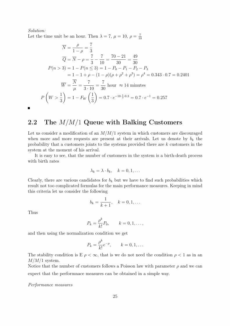
Solution:Let the time unit be an hour. Then λ = 7, µ = 10, ρ = 7
10
N =ρ
1− ρ=
7
3
Q = N − ρ =7
3− 7
10=
70− 21
30=
49
30P (n > 3) = 1− P (n ≤ 3) = 1− P0 − P1 − P2 − P3
= 1− 1 + ρ− (1− ρ)(ρ+ ρ2 + ρ3) = ρ4 = 0.343 · 0.7 = 0.2401
W =N
µ=
7
3 · 10=
7
30hour ≈ 14 minutes
P
(W >
1
3
)= 1− FW
(1
3
)= 0.7 · e−10· 1
3·0.3 = 0.7 · e−1 = 0.257
2.2 The M/M/1 Queue with Balking CustomersLet us consider a modification of an M/M/1 system in which customers are discouragedwhen more and more requests are present at their arrivals. Let us denote by bk theprobability that a customers joints to the systems provided there are k customers in thesystem at the moment of his arrival.
It is easy to see, that the number of customers in the system is a birth-death processwith birth rates
λk = λ · bk, k = 0, 1, . . .
Clearly, there are various candidates for bk but we have to find such probabilities whichresult not too complicated formulas for the main performance measures. Keeping in mindthis criteria let us consider the following
bk =1
k + 1, k = 0, 1, . . .
Thus
Pk =ρk
k!P0, k = 0, 1, . . . ,
and then using the normalization condition we get
Pk =ρk
k!e−ρ, k = 0, 1, . . .
The stability condition is E ρ <∞, that is we do not need the condition ρ < 1 as in anM/M/1 system.Notice that the number of customers follows a Poisson law with parameter ρ and we can
expect that the performnace measures can be obtained in a simple way.
Performance measures
25
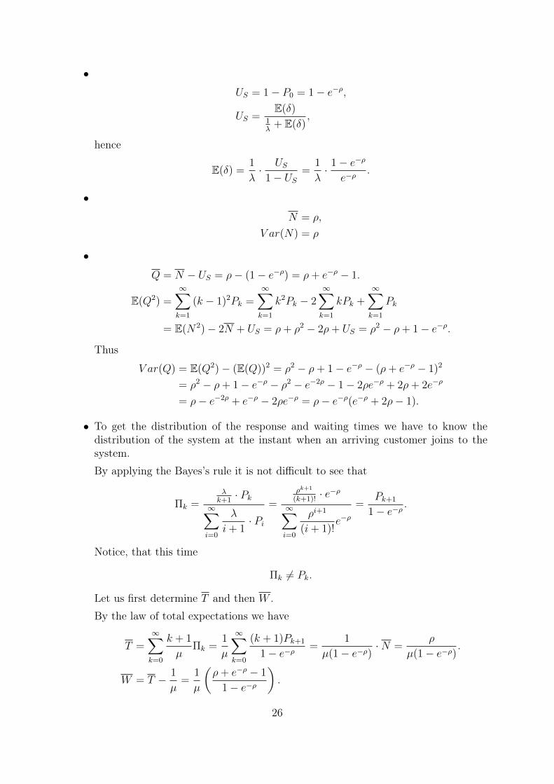
•US = 1− P0 = 1− e−ρ,
US =E(δ)
1λ
+ E(δ),
hence
E(δ) =1
λ· US
1− US=
1
λ· 1− e−ρ
e−ρ.
•
N = ρ,
V ar(N) = ρ
•
Q = N − US = ρ− (1− e−ρ) = ρ+ e−ρ − 1.
E(Q2) =∞∑k=1
(k − 1)2Pk =∞∑k=1
k2Pk − 2∞∑k=1
kPk +∞∑k=1
Pk
= E(N2)− 2N + US = ρ+ ρ2 − 2ρ+ US = ρ2 − ρ+ 1− e−ρ.
Thus
V ar(Q) = E(Q2)− (E(Q))2 = ρ2 − ρ+ 1− e−ρ − (ρ+ e−ρ − 1)2
= ρ2 − ρ+ 1− e−ρ − ρ2 − e−2ρ − 1− 2ρe−ρ + 2ρ+ 2e−ρ
= ρ− e−2ρ + e−ρ − 2ρe−ρ = ρ− e−ρ(e−ρ + 2ρ− 1).
• To get the distribution of the response and waiting times we have to know thedistribution of the system at the instant when an arriving customer joins to thesystem.
By applying the Bayes’s rule it is not difficult to see that
Πk =λk+1· Pk
∞∑i=0
λ
i+ 1· Pi
=
ρk+1
(k+1)!· e−ρ
∞∑i=0
ρi+1
(i+ 1)!e−ρ
=Pk+1
1− e−ρ.
Notice, that this time
Πk 6= Pk.
Let us first determine T and then W .
By the law of total expectations we have
T =∞∑k=0
k + 1
µΠk =
1
µ
∞∑k=0
(k + 1)Pk+1
1− e−ρ=
1
µ(1− e−ρ)·N =
ρ
µ(1− e−ρ).
W = T − 1
µ=
1
µ
(ρ+ e−ρ − 1
1− e−ρ
).
26
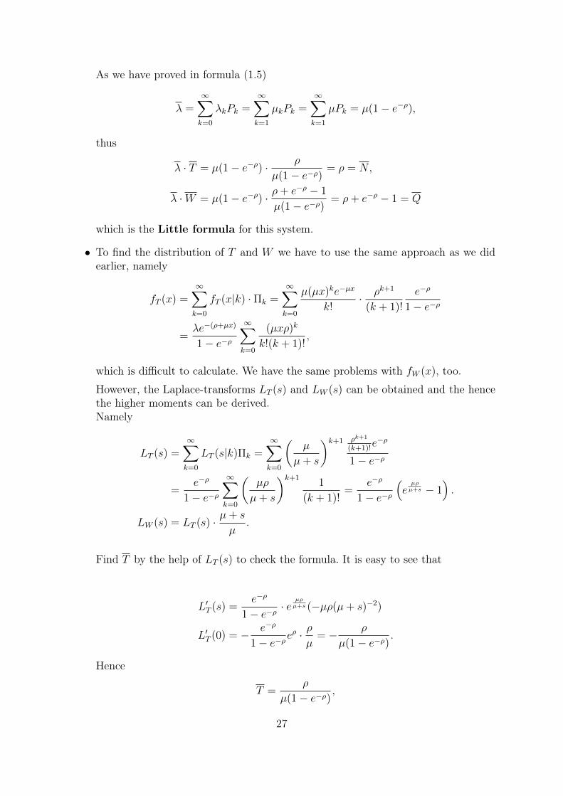
As we have proved in formula (1.5)
λ =∞∑k=0
λkPk =∞∑k=1
µkPk =∞∑k=1
µPk = µ(1− e−ρ),
thus
λ · T = µ(1− e−ρ) · ρ
µ(1− e−ρ)= ρ = N,
λ ·W = µ(1− e−ρ) · ρ+ e−ρ − 1
µ(1− e−ρ)= ρ+ e−ρ − 1 = Q
which is the Little formula for this system.
• To find the distribution of T and W we have to use the same approach as we didearlier, namely
fT (x) =∞∑k=0
fT (x|k) · Πk =∞∑k=0
µ(µx)ke−µx
k!· ρk+1
(k + 1)!
e−ρ
1− e−ρ
=λe−(ρ+µx)
1− e−ρ∞∑k=0
(µxρ)k
k!(k + 1)!,
which is difficult to calculate. We have the same problems with fW (x), too.
However, the Laplace-transforms LT (s) and LW (s) can be obtained and the hencethe higher moments can be derived.Namely
LT (s) =∞∑k=0
LT (s|k)Πk =∞∑k=0
(µ
µ+ s
)k+1 ρk+1
(k+1)!e−ρ
1− e−ρ
=e−ρ
1− e−ρ∞∑k=0
(µρ
µ+ s
)k+11
(k + 1)!=
e−ρ
1− e−ρ(eµρµ+s − 1
).
LW (s) = LT (s) · µ+ s
µ.
Find T by the help of LT (s) to check the formula. It is easy to see that
L′T (s) =e−ρ
1− e−ρ· e
µρµ+s (−µρ(µ+ s)−2)
L′T (0) = − e−ρ
1− e−ρeρ · ρ
µ= − ρ
µ(1− e−ρ).
Hence
T =ρ
µ(1− e−ρ),
27
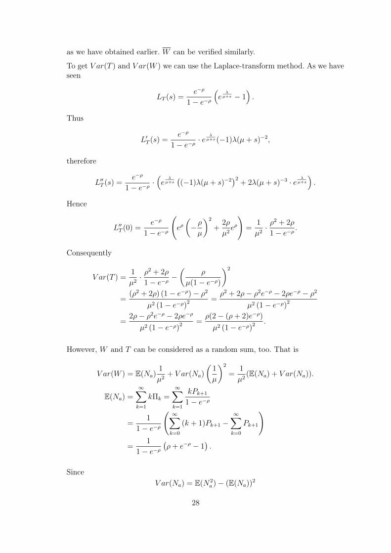
as we have obtained earlier. W can be verified similarly.
To get V ar(T ) and V ar(W ) we can use the Laplace-transform method. As we haveseen
LT (s) =e−ρ
1− e−ρ(e
λµ+s − 1
).
Thus
L′T (s) =e−ρ
1− e−ρ· e
λµ+s (−1)λ(µ+ s)−2,
therefore
L′′T (s) =e−ρ
1− e−ρ·(e
λµ+s((−1)λ(µ+ s)−2
)2+ 2λ(µ+ s)−3 · e
λµ+s
).
Hence
L′′T (0) =e−ρ
1− e−ρ
(eρ(−ρµ
)2
+2ρ
µ2eρ
)=
1
µ2· ρ
2 + 2ρ
1− e−ρ.
Consequently
V ar(T ) =1
µ2· ρ
2 + 2ρ
1− e−ρ−(
ρ
µ(1− e−ρ)
)2
=(ρ2 + 2ρ) (1− e−ρ)− ρ2
µ2 (1− e−ρ)2 =ρ2 + 2ρ− ρ2e−ρ − 2ρe−ρ − ρ2
µ2 (1− e−ρ)2
=2ρ− ρ2e−ρ − 2ρe−ρ
µ2 (1− e−ρ)2 =ρ(2− (ρ+ 2)e−ρ)
µ2 (1− e−ρ)2 .
However, W and T can be considered as a random sum, too. That is
V ar(W ) = E(Na)1
µ2+ V ar(Na)
(1
µ
)2
=1
µ2(E(Na) + V ar(Na)).
E(Na) =∞∑k=1
kΠk =∞∑k=1
kPk+1
1− e−ρ
=1
1− e−ρ
(∞∑k=0
(k + 1)Pk+1 −∞∑k=0
Pk+1
)=
1
1− e−ρ(ρ+ e−ρ − 1
).
SinceV ar(Na) = E(N2
a )− (E(Na))2
28

first we have to calculate E(N2a ), that is
E(N2a ) =
∞∑k=1
k2Πk =∞∑k=1
k2 Pk+1
1− e−ρ
=1
1− e−ρ∞∑k=0
((k + 1)2 − 2k − 1
)Pk+1
=1
1− e−ρ
(∞∑k=0
(k + 1)2Pk+1 − 2∞∑k=0
kPk+1 −∞∑k=0
Pk+1
)=
1
1− e−ρ(ρ+ ρ2 − 2
(ρ+ e−ρ − 1
)−(1− e−ρ
))=
1
1− e−ρ(ρ2 − ρ− e−ρ + 1
).
Therefore
V ar(Na) =1
1− e−ρ(ρ2 − ρ− e−ρ + 1
)−(
1
1− e−ρ(ρ+ e−ρ − 1)
)2
=
(1
1− e−ρ
)2 ((1− e−ρ)
(ρ2 − ρ− e−ρ + 1
)−(ρ+ e−ρ − 1
)2)
=
(1
1− e−ρ
)2
(ρ2 − ρ− e−ρ + 1− ρ2e−ρ + ρe−ρ + e−2ρ − e−ρ
− ρ2 − e−2ρ − 1− 2ρe−ρ + 2ρ− 2e−ρ)
=ρ− e−ρ(ρ2 + ρ)
(1− e−ρ)2.
Finally
V ar(W ) =
(1
µ
)2(1
1− e−ρ(ρ+ e−ρ − 1) +
ρ− e−ρ(ρ2 + ρ)
(1− e−ρ)2
)=
1
(µ(1− e−ρ))2((ρ+ e−ρ − 1)(1− e−ρ) + ρ− e−ρ(ρ2 + ρ)).
Thus
V ar(T ) = V ar(W ) +1
µ2
V ar(T ) =
(1
µ(1− e−ρ)
)2
(ρ+ e−ρ − 1)(1− e−ρ) + ρ− e−ρ(ρ2 + ρ) + (1− e−ρ)2)
=(1− e−ρ)(ρ+ e−ρ − 1 + 1− e−ρ) + ρ− e−ρ(ρ2 + ρ)
(µ(1− e−ρ))2
=2ρ− 2ρe−ρ − ρ2e−ρ
(µ(1− e−ρ)2
which is the same we have obtained earlier.
29

2.3 Priority M/M/1 QueuesIn the following let us consider an M/M/1 systems with priorities. This means that wehave two classes of customers. Each type of requests arrive according to a Poisson processwith parameter λ1, and λ2, respectively and the processes are supposed to be independentof each other. The service times for each class are assumed to be exponentially distributedwith parameter µ. The system is stable if
ρ1 + ρ2 < 1,
where ρi = λi/µ, i = 1, 2.Let us assume that class 1 has priority over class 2. This section is devoted to the investi-gation of preemptive and non-preemptive systems and some mean values are calculated.
Preemptive Priority
According to the discipline the service of a customer belonging to class 2 is never carriedout if there is customer belonging to class 1 in the system. In other words it means thatclass 1 preempts class 2 that is if a class 2 customer is under service when a class 1 requestarrives the service stops and the service of class 1 request starts. The interrupted serviceis continued only if there is no class 1 customer in the system.
Let Ni denote the number of class i customers in the system and let Ti stand for theresponse time of class i requests. Our aim is to calculate E(Ni) and E(Ti) for i = 1, 2.Since type 1 always preempts type 2 the service of class 1 customers is independent ofthe number of class 2 customers. Thus we have
(2.3) E(T1) =1/µ
1− ρ1
, E(N1) =ρ1
1− ρ1
.
Since for all customers the service time is exponentially distributed with the same pa-rameter, the number of customers does not depends on the order of service. Hence forthe total number of customers in an M/M/1 we get
(2.4) E(N1) + E(N2) =ρ1 + ρ2
1− ρ1 − ρ2
,
and then inserting (2.3) we obtain
E(N2) =ρ1 + ρ2
1− ρ1 − ρ2
− ρ1
1− ρ1
=ρ2
(1− ρ1)(1− ρ1 − ρ2),
and using the Little’s law we have
E(T2) =E(N2)
λ2
=1/µ
(1− ρ1)(1− ρ1 − ρ2).
Example 2 Let us compare what is the difference if preemptive priority discipline is ap-plied instead of FIFO.
30

Let λ1 = 0.5, λ2 = 0.25 and µ = 1. In FIFO case we get
E(T ) = 4.0, E(W ) = 3.0, E(N) = 3.0
and in priority case we obtain
E(T1) = 2.0, E(W1) = 1.0, E(N1) = 1.0
E(T2) = 8.0, E(W2) = 6.0, E(N2) = 2.0
Non-preemptive Priority
The only difference between the two disciplines is that in the case the arrival of a class1 customer does not interrupt the service of type 2 request. That is why sometimes thisdiscipline is call HOL ( Head Of the Line ). Of course after finishing the service of class1 starts.
By using the law of total expectations the mean response time for class 1 can be obtainedas
E(T1) = E(N1)1
µ+
1
µ+ ρ2
1
µ.
The last term shows the situation when an arriving class 1 customer find the serverbusy servicing a class 2 customer. Since the service time is exponentially distributed theresidual service time has the same distribution as the original one. Furthermore, becauseof the Poisson arrivals the distribution at arrival moments is the same as at randommoments, that is the probability that the server is busy with class 2 customer is ρ2. Byusing the Little’s law
E(N1) = λ1E(T1),
after substitution we get
E(T1) =(1 + ρ2)/µ
1− ρ1
, E(N1) =(1 + ρ2)ρ1
1− ρ1
.
To get the means for class 2 the same procedure can be performed as in the previouscase. That is using (2.4) after substitution we obtain
E(N2) =(1− ρ1(1− ρ1 − ρ2))ρ2
(1− ρ1)(1− ρ1 − ρ2),
and then applying the Little’s law we have
E(T2) =(1− ρ1(1− ρ1 − ρ2))/µ
(1− ρ1)(1− ρ1 − ρ2).
31

Example 3 Now let us compare the difference between the two priority disciplines.Let λ1 = 0.5, λ2 = 0.25 and µ = 1, then
E(T1) = 2.5, E(W1) = 1.5, E(N1) = 1.25
E(T2) = 7.0, E(W2) = 6.0, E(N2) = 1.75
Of course knowing the mean response time and mean number of customers in the systemthe mean waiting time and the mean number of waiting customers can be obtained inthe usual way.
Java applets for direct calculations can be found athttp://irh.inf.unideb.hu/user/jsztrik/education/03/EN/MMcPrio/MMcPrio.html
http://www.win.tue.nl/cow/Q2/
2.4 The M/M/1/K Queue, Systems with Finite Capac-ity
LetK be the capacity of anM/M/1 system, that is the maximum number of customers inthe system including the one under service. It is easy to see that the nu,ber of customersin the systems is a birth-death process with rates λk = λ, k = 0, . . . , K − 1 és µk = µ,k = 1, . . . , K. For the steady-state distribution we have
Pk =ρk
K∑i=0
ρi
, k = 0, . . . , K,
that is
P0 =1
K∑i=0
ρi
=
1
K+1, ρ = 1
1−ρ1−ρK+1 , ρ 6= 1.
It sholud be noted that the system is stable for any ρ > 0 when K is fixed. However, ifK →∞ the the stability condition is ρ < 1 since the distribution ofM/M/1/K convergesto the distribution of M/M/1.It can be verified analytically since ρK → 0 then P0 → 1− ρ.
Similarly to anM/M/1 systems after reasonable modifications the performance measurescan be computed as
•US = 1− P0,
E(δ) =1
λ
US1− US
32

•
N =K∑k=1
kρkP0 = ρP0
K∑k=1
kρk−1
= ρP0
(K∑k=1
ρk
)′= ρP0
(ρ
1− ρK
1− ρ
)′= ρP0
(ρ− ρK+1
1− ρ
)′=((
1− (K + 1)ρK)
(1− ρ) + ρ− ρK+1)· ρP0
(1− ρ)2
=ρP0
(1− (K + 1)ρK − ρ+ (K + 1)ρK+1 + ρ− ρK+1
)(1− ρ)2
=ρP0
(1− (K + 1)ρK +KρK+1
)(1− ρ)2
=ρ(1− (K + 1)ρK +KρK+1
)(1− ρ)(1− ρK+1)
.
•
Q =K∑k=1
(k − 1)Pk =K∑k=1
kPk −K∑k=1
Pk = N − US
• To obtain the distribution of the response and waiting time we have to know thedistribution of the system at the moment when the tagged customer enters intoto system. It should be underlined that the customer should enter into the systemand it is not the same as an arriving customer. An arriving customer can join thesystem or can be lost because the system is full. By using the Bayes’ theorem it iseasy to see that
Πk =λPk
K−1∑i=0
λPi
=Pk
1− PK.
Similarly to the investigations we carried out in an M/M/1 system the mean andthe density function of the response time can be obtained by the help of the law oftotal means and law of total probability, respectively.
For the expectation we have
T =K−1∑k=0
k + 1
µΠk =
K−1∑k=0
k + 1
µ
ρkP0
1− Pk
=1
λ(1− PK)
K−1∑k=0
(k + 1)Pk+1 =N
λ(1− PK).
33
Consequently
W = T − 1
µ=
N
λ(1− PK)− 1
µ.
We would like to show that the Little’s law is valid in this case and the same timewe can check the correctness of the formula.It can easily be seen that the average arrival rate into the system is λ = λ(1− PK)and thus
λ · T = λ(1− PK)N
λ(1− PK)= N.
Similarly
λ ·W = λ
(N
λ(1− PK)− 1
µ
)= N − λ
µ
= N − ρ(1− PK) = N − US = Q,
since
λ = µ = µUS.
Now let us find the density function of the response and waiting timesBy using the theorem of total probability we have
fT (x) =K−1∑k=0
µ(µx)k
k!e−µx
Pk1− PK
,
and thus for the distribution function we get
FT (x) =K−1∑k=0
x∫0
µ(µt)k
k!e−µtdt
Pk1− PK
=K−1∑k=0
(1−
k∑i=0
(µx)i
i!e−µx
)Pk
1− PK
= 1−K−1∑k=0
(k∑i=0
(µx)i
i!e−µx
)Pk
1− PK.
Thes formulas are more complicated due to the finite summation as in the case ofan M/M/1 system, but it is not difficult to see that in the limiting case as K →∞we have
fT (x) = µ(1− ρ)e−µ(1−ρ)x.
34

For the density and distribution function of the waiting time we obtain
fW (0) =P0
1− PK
fW (x) =K−1∑k=1
µ(µx)k−1
(k − 1)!e−µx
Pk1− PK
, x > 0
FW (x) =P0
1− PK+
K−1∑k=1
(1−
k−1∑i=0
(µx)i
i!e−µx
)Pk
1− PK
= 1−K−1∑k=1
(k−1∑i=0
(µx)i
i!e−µx
)· Pk
1− PK.
These formulas can be calculated very easily by a computer.As we can see the probability PK plays an important role in the calculations.Notice that it is exactly the probability that an arriving customer find the systemfull that is it lost. It is called blocking or lost probability and denoted by PB.Its correctness can be proved by the help of the Bayes’s rule, namely
PB =λPKK∑k=0
λPk
= PK .
If we would like to show the dependence on K and ρ it can be denoted by
PB(K, ρ) =ρK
K∑k=0
ρk
.
Notice that
PB(K, ρ) =ρρK−1
K−1∑k=0
ρk + ρρK−1
=ρPB(K − 1, ρ)
1 + ρPB(K − 1, ρ).
Starting with the initial value PB(1, ρ) =ρ
1 + ρthe probability of loss can be com-
puted recursively. It is obvious that this sequence tends to 0 as ρ < 1. Consequentlyby using the recursion we can always find an K-t, for which
PB(K, ρ) < P ∗,
where P ∗ is a predefined limit value for the probability of loss.
To find the value of K without recursion we have to solve the inequality
ρK(1− ρ)
1− ρK+1< P ∗
35
which is more complicated task.
Alternatively can can find an approximation method, too. Use the distribution ofan M/M/1 system and find the probability that in the system there are at least Kcustomers. It is easy to see that
PB(K, ρ) =ρK(1− ρ)
1− ρK+1<
∞∑k=K
ρk(1− ρ) = ρK ,
and thus if
ρK < P ∗,
then P ∗B(K, ρ) < P ∗. That is
K ln ρ < lnP ∗
K >lnP ∗
ln ρ.
Now let us turn our attention to the Laplace-transform of the response and wait-ing times. First let us compute it for the response time. Similarly to the previousarguments we have
LT (s) =K−1∑k=0
(µ
µ+ s
)k+1ρkP0
1− PK
=P0
ρ(1− PK)
K∑l=1
(µρ
µ+ s
)l
=P0
ρ(1− PK)
λ
µ+ s
1−(
λµ+s
)K1− λ
µ+s
=µP0
(1− PK)
1−(
λµ+s
)Kµ− λ+ s
.
The Laplace-transform of the waiting time can be obtained as
LW (s) =K−1∑k=0
(µ
µ+ s
)kρkP0
1− PK
=P0
1− PK
K−1∑k=0
(µρ
µ+ s
)k
=P0
1− PK
1−(
λµ+s
)K1− λ
µ+s
=P0
1− PK
(µ+ s)
(1−
(λµ+s
)K)µ− λ+ s
,
36

which also follows from relation
LT (s) = LW (s) · µ
µ+ s.
By the help of the Laplace-transforms the higher moments of the involved randomvariables can be computed, too.
Java applets for direct calculations can be found athttp://irh.inf.unideb.hu/user/jsztrik/education/03/EN/MM1K/MM1K.html
2.5 The M/M/∞ Queue
Similarly to the previous systems it is easy to see that the number of customers in thesystem, that is the process (N(t), t ≥ 0) is a birth-death process with rates
λk = λ, k = 0, 1, . . .
µk = kµ, k = 1, 2, . . . .
Hence the steady-state distribution can be obtained as
Pk =%k
k!P0, where P−1
0 =∞∑k=0
%k
k!= e%,
That is
Pk =%k
k!e−%,
showing that N follows a Poisson law with parameter %.
It is easy to see that the performance measures can be computed as
N = %, λ = λ, T =1
µ, W = 0, r = N, µ = rµ
Ur = 1− e−%, E(δr)1λ
=1− e−%
e−%, E(δr) =
1
λ
1− e−%
e−%.
It can be proved that these formulas remain valid for an M/G/∞ system as well where
E(S) =1
µ.
Java applets for direct calculations can be found athttp://irh.inf.unideb.hu/user/jsztrik/education/03/EN/MMinf/MMinf.html
37
2.6 The M/M/n/n Queue, Erlang-Loss SystemThis system is the oldest and thus the most famous system in queueing theory. The ori-gin of the traffic theory or congestion theory started by the investigation of this systemand Erlang was the first who obtained his well-reputed formulas, see for example Erlang[21, 22].By assumptions customers arrive according to a Poisson process and the service timesare exponentially distributed. However, if n servers all busy when a new customer arrivesit will be lost because the system is full. The most important question is what proportionof the customers is lost.
The process (N(t), t ≥ 0) is said to be in state k if k servers are busy, which is the same ask customers are in the system. It is easy to see that (N(t), t ≥ 0)is a birth-death processwith rates
λk =
{λ, if k < n,0, if k ≥ n,
µk = kµ, k = 1, 2, ..., n.
Clearly the steady-state distribution exists since the process has a finite state space. Thestationary distribution can be obtained as
Pk =
P0
(λ
µ
)k1
k!, if k ≤ n,
0 , if k > 0.
Due to the normalizing condition we have
P0 =
(n∑k=0
(λ
µ
)k1
k!
)−1
,
and thus the distribution is
Pk =
(λ
µ
)k1
k!n∑i=0
(λ
µ
)i1
i!
=
%k
k!n∑i=0
%i
i!
, k ≤ n.
The most important measure of the system is
Pn =
%n
n!n∑k=0
%k
k!
= B(n, ρ)
which was introduced by Erlang and it is referred to as Erlang’s B-formula, or lossformula and generally denoted by B(n, λ/µ).
38

By using the Bayes’s rule it is easy to see that Pn is the probability that an arrivingcustomer is lost. For moderate n the probability P0 can easily be computed. For large n
and small % P0 ≈ e−%, and thus
Pk ≈%k
k!e−%,
that is the Poisson distribution. For large n and large %
n∑j=0
%j
j!6= e%.
However, in this case the central limit theorem can be used, since the denominator is thesum of the first (n+ 1) terms of a Poisson distribution with mean %. Thus by the centrallimit theorem this Poisson distribution can be approximated by a normal law with mean% and variance √% that is
Pn ≈Φ(s)− Φ(s− 1/
√%)
Φ(s)= 1−
Φ(s− 1/√%)
Φ(s),
where
Φ(s) =
s∫−∞
1√2πe−
x2
2 dx,
and
s =n+ 1
2− %
√%
.
Another way to calculate B(n, ρ) is to find a recursion. This can be obtained as follows
B(n, p) =ρn
n!n∑i=0
ρi
i!
=
ρnρn−1
(n−1)!
n∑i=0
ρi
i!+ρ
n
ρn−1
(n− 1)!
=ρnB(n− 1, ρ)
1 + ρnB(n− 1, ρ)
=ρB(n− 1, ρ)
n+ ρB(n− 1, ρ).
Using B(1, ρ) =ρ
1 + ρas an initial value the probabilities B(n, ρ) can be computed for
any n. It is important since the direct calculation can cause a problem due to the valueof the factorial.For example for n = 1000, ρ = 1000 the exact formula cannot be computed but the ap-proximation and the recursion gives the value 0.024.
Due to the great importance of B(n, ρ) in practical problems so-called calculators havebeen developed which can be found at
http://www.erlang.com/calculator/
39

To compare the approximations and the exact values we also have developed our ownJava script which can be used at
http://jani.uw.hu/erlang/erlang.html
Now determine the main performance measures of this M/M/n/n system
• Mean number of customers in the systems, mean number of busy servers
N = n =n∑j=0
jPj =n∑j=0
j%j
j!P0 = %
n−1∑j=0
%i
i!P0 = %(1− Pn),
thus the mean number of requests for a given server is%
n(1− Pn).
• Utilization of a server
As we have seen
Us =n∑i=1
i
nPi =
n̄
n.
This caseUs =
%
n(1− Pn).
• The mean idle period for a given server
By applying the well-known relation
P (the server is idle ) =1/µ
e+ 1/µ,
where e is the mean idle time of the server. Thus
%
n(1− Pn) =
1/µ
e+ 1/µ,
hencee =
n
λ(1− Pn)− 1
µ.
• The mean busy period of the system
Clearly
Ur = 1− P0 =Eδr
1λ
+ Eδr,
thus
Eδr =1− P0
λP0
=
n∑i=1
%i
i!
λ
(1 +
n∑i=1
%i
i!
) .
40

Java applets for direct calculations can be found athttp://irh.inf.unideb.hu/user/jsztrik/education/03/EN/MMcc/MMcc.html
Example 4 In busy parking lot cars arrive according to a Poisson process one in 20seconds and stay there in the average of 10 minutes.How many parking places are required if the probability of a loss is no to exceed 1% ?
Solution:ρ =
λ
µ=
1013
= 30, Pn = 0.01.
Following a normal approximation
Pn = 0.01 =ρn
n!e−ρ
Φ(n+ 1
2−ρ
√ρ
) =Φ(n+ 1
2−ρ
√ρ
)− Φ
(n− 1
2−ρ
√ρ
)Φ(n+ 1
2−ρ
√ρ
) .
Thus
0.99Φ
(n+ 1
2− ρ
√ρ
)= Φ
(n− 1
2− ρ
√ρ
).
It is not difficult to verify by using the Table for the standard normal distribution thatn = 41.
Thus the approximation value of P41 is 0.009917321712214377,and the exact value is 0.01043318100246811.
Example 5 A telephone exchange consists of 50 lines and calls arrive according to aPoisson process, the mean interarrival time is 10 minutes. The mean service time is 5minutes.Find the main performance measures.
Solution:Using Poisson approximation where ρ = λ
µ= 0.5
P50 = 0.00000, event for n = 6P6 = 0, 00001. This means that a call is almost never lost.Mean number of busy lines can be obtain as
n = ρ(1− Pn) = ρ = 0.5 ,
The utilization of a line is
0.5
50=
5× 10⁻¹
5× 10= 10−2
The utilization of the system is
Ur = 1− 0.606 = 0.394
41
The mean busy period of the system can be obtained as
Eδr =(1− P0)
(λP0)=
0.394
2× 0.606=
0.394
1.212= 0.32 minutes
Mean idle period of a line is
e =n
λ(1− Pn)− ρ
λ=
50
2(1− 0)− 0, 5
2= 25− 1
4= 24.75 minutes
Heterogeneous Servers
In the case of an M/−→M/n/n system the service time distribution depends on the index
of the server. That is the service time is exponentially distributed with parameter µi forserver i. An arriving customer choose randomly among the idle servers, that is each idleserver is chosen with the same probability. Since the servers are heterogeneous it is notenough to to the number of busy servers but we have to identify them by their index. Itmeans that we have to deal with general Markov-processes.
Let (i1, . . . , ik) denote the indexes of the busy servers, which are the combinations of nobjects taken k at a time without replacement. Thus the state space of the Markov-chainis the set of these combinations, that is (0, (i1, . . . , ik) ∈ Cn
k , k = 1, . . . , n).
Let us denote by
P0 = P (0),
P (i1, . . . , ik) = P ((i1, . . . , ik)), (i1, . . . , ik) ∈ Cnk , k = 1, . . . , n
the steady-state distribution of the chain which exists since the chain has a finite statespace and it is irreducible. The set of steady-state balance equations can be written as
(2.5) λP0 =n∑j=1
µjP (j)
(λ+k∑j=1
µij)P (i1, . . . , ik) =λ
n− k + 1
k∑j=1
P (i1, . . . , ij−1, ij+1, . . . , ik)
+∑
j 6=i1,...,ik
µjP (i′1, . . . , i′k, j′)
(2.6)
(2.7)( n∑j=1
µj
)P (1, . . . , n) = λ
n∑j=1
P (1, . . . , j − 1, j + 1, . . . , n)
42
where (i′1, . . . , i′k, j′) denotes the ordered set i1, . . . , ik, j, i−1 and in+1 are not defined.
Despite of the large number of unknowns, which is 2n, the solution is quite simple, namely
(2.8) P (i1, . . . , ik) = (n− k)!k∏j=1
%ijC,
where %j =λ
µi, j = 1, . . . , n, P0 = n!C, which can be determined by the help of the
normalizing condition
P0 +n∑k=1
∑(i1,...,ik)∈Cnk
P (i1, . . . , ik) = 1.
Let us check the first equation (2.5). By substitution we have
λn!C =n∑j=1
µjλ
µj(n− 1)!C = n!λC.
Lets us check now the third equation (2.7)
( n∑j=1
µj
)λn
µ1 · · ·µnC = λ
n∑j=1
λn−1C
µ1 · · ·µj−1µj+1 · · ·µn=
λn
µ1 · · ·µn
( n∑j=1
µj
)C.
Finally let us check the most complicated one, the second set of equations (2.6), namely
(λ+k∑j=1
µij)(n− k)!k∏j=1
%ijC
=λ
n− k + 1(n− k + 1)!
k∑j=1
λk−1C
µi1 · · ·µij−1µij+1
· · ·µik
+∑
j 6=i1,...,ik
(n− k − 1)!λk+1µjC
µi1 · · ·µikµj
= (n− k)!k∑j=1
µijλkC
µi1 · · ·µik+ λ
∑j 6=i1,...,ik
(n− k − 1)!λkC
µi1 · · ·µik
= (n− k)!
( k∑j=1
µij
)λkC
µi1 · · ·µik+ λ(n− k)!
λkC
µi1 · · ·µik,
which shows the equality.
Thus the usual performance measures can be obtained as
43
• the utilization of the jth server Uj can be calculated as
Uj =n∑k=1
∑j∈(i1,...,ik)
P (i1, . . . , ik),
and thus
Uj =
1µj
1µj
+ E(ej),
where E(ej) is the mean idle period of the jth server. Hence
E(ej) =1
µj
1− UjUj
.
• N =∑n
j=1 Uj
• The probability of loss is PB = P (1, . . . , n).
It should be noted that in this case the following relation also holds
λ(1− PB) =n∑j=1
Ujµj.
In homogeneous case, that is when µj = µ, j = 1, . . . , n, after substitution we have
Pk =∑
(i1,...,ik)∈Cnk
P (i1, . . . , ik) =
(n
k
)(n− k)!%kC =
%k
k!n!C =
%k
k!P0 =
%k
k!∑nj=1
%j
j!
,
that is it reduces to the Erlang’s formula derived earlier.
It should be noted that these formulas remains valid under generally distributed servicetimes with finite means with ρi = λE(Si). In other words the Erlang’s loss formula isrobust to the distribution of the service time, it does not depend on the distribution itselfbut only on its mean.
2.7 The M/M/n Queue
It is a variation of the classical queue assuming that the service is provided by n serversoperating independently of each other. This modification is natural since if the meanarrival rate is greater than the service rate the system will not be stable, that is whythe number of servers should be increased. However, in this situation we have parallelservices and we are interested in the distribution of first service completion.That is why we need the following observation.
44

Let Xi be exponentially distributed random variables with parameter µi, (i = 1, 2, ..., r)and denote by Y their minimum. It is not difficult to see that Y is also exponentially
distributed with parameterr∑i=1
µi since
P (Y < x) = 1− P (Y ≥ x) = 1− P (Xi ≥ x, i = 1, ..., r) =
= 1−r∏i=1
P (Xi ≥ x) = 1− e−(∑ri=1 µi)x.
Similarly to the earlier investigations, it can easily be verified that the number of cus-tomers in the system is a birth-death process with the following transition probabilities
Pk,k−1(h) = (1− (λh+ o(h))) (µkh+ o(h)) + o(h) = µkh+ o(h),
Pk,k+1(h) = (λh+ o(h)) (1− (µkh+ o(h))) + o(h) = λh+ o(h),
where
µk = min(kµ, nµ) =
kµ , for 0 ≤ k ≤ n,
nµ , for n < k.
It is understandable that the stability condition is λ/nµ < 1.
To obtain the distribution Pk we have to distinguish two cases according to as µk dependson k. Thus if k < n, then we get
Pk = P0
k−1∏i=0
λ
(i+ 1)µ= P0
(λ
µ
)k1
k!.
Similarly, if k ≥ n, then we have
Pk = P0
n−1∏i=0
λ
(i+ 1)µ
k−1∏j=n
λ
nµ= P0
(λ
µ
)k1
n!nk−n.
In summary
Pk =
P0ρk
k!, for k ≤ n,
P0aknn
n!, for k > n,
wherea =
λ
nµ=ρ
n< 1.
This a is exactly the utilization of a given server . Furthermore
P0 =
(1 +
n−1∑k=1
ρk
k!+∞∑k=n
ρk
n!
1
nk−n
)−1
,
45

and thus
P0 =
(n−1∑k=0
ρk
k!+ρn
n!
1
1− a
)−1
.
Since the arrivals follow a Poisson law the the distribution of the system at arrival instantsequals to the distribution at random moments, hence the probability that an arrivingcustomer has to wait is
P (waiting) =∞∑k=n
Pk =∞∑k=n
P0ρk
n!
1
nk−n.
that is it can be written as
P (waiting) =
ρn
n!
1
1− an−1∑k=0
ρk
k!+ρn
n!
1
1− a
=
ρn
n!nn−ρ
n−1∑k=0
ρk
k!+
ρnn
n!(n− ρ)
= C(n, ρ).
This probability is frequently used in different practical problems, for example in tele-phone systems, call centers, just to mention some of them. It is also a very famous formulawhich is referred to as Erlang’s C formula,or Erlang’s delay formula and it is de-noted by C(n, λ/µ).
The main performance measures of the systems can be obtained as follows
• For the mean queue length we have
Q =∞∑k=n
(k − n)Pk =∞∑j=0
jPn+j =∞∑j=0
j(λµ
)n+j
n!njP0 =
=∞∑j=0
j
(λµ
)nn!
ajP0 = P0
(λµ
)nn!
a
∞∑j=0
daj
da= P0
(λµ
)nn!
ad
da
∞∑j=0
aj =
= P0
(λµ
)nn!
a
(1− a)2=
ρ
n− ρC(n, ρ).
• For the mean number of busy servers we obtain
n =n−1∑k=0
kPk +∞∑k=n
nPk = P0
(ρn−2∑k=0
ρk
k!+
ρn
(n− 1)!
1
1− a
)=
= ρ
(n−2∑k=0
ρk
k!+
ρn−1
(n− 1)!+
ρn−1
(n− 1)!
(1
1− a− 1
))P0 =
= ρ
(n−1∑k=0
ρk
k!+ρn
n!
1
1− a
)P0 = ρ
1
p0
P0 = ρ.
46
• For the mean number of customers in the system we get
N =∞∑k=0
kPk =n−1∑k=0
kPk +∞∑k=n
(k − n)Pk +∞∑k=n
nPk = n+Q
= ρ+ρ
n− ρC(n, ρ),
which is understandable since a customer is either in the queue or in service. Letus denote by S-gal the mean number of idle servers. Then it is easy to see that
n = n− S,
S = n− λ
µ,
thusN = n− S +Q,
henceN − n = Q− S.
• Distribution of the waiting time
An arriving customer has to wait if at his arrival the number of customers in thesystem is at least n. In this case the time while a customer is serviced is exponentiallydistributed with parameter nµ, consequently if there n+ j customers in the systemthe waiting time is Erlang distributed with parameters (j+ 1, nµ). By applying thetheorem of total probability for the density function of the waiting time we have
fW (x) =∞∑j=0
Pn+j(nµ)j+1xj
j!e−nµx.
Substituting the distribution we get
fW (x) =∞∑j=0
P0
(λµ
)nn!
aj(nµ)j+1xj
j!e−nµx
=P0
(λµ
)nn!
nµe−nµx∞∑j=0
(anµx)j
j!
=
(λµ
)nn!
P0nµe−(nµ−λ)x
=
(λµ
)nn!
P0nµe−nµ(1−a)x
=
(λµ
)nn!
P01
1− anµ(1− a)e−nµ(1−a)x
= P (waiting)nµ(1− a)e−nµ(1−a)x.
47

Hence for the complement of the distribution function we obtain
P (W > x) =
∞∫x
fW (u)du = P (waiting)e−nµ(1−a)x
= C(n, ρ) · e−µ(n−ρ)x.
Therefore the distribution function can be written as
FW (x) = 1− P (waiting) + P (waiting)(1− e−nµ(1−a)x
)= 1− P (waiting)e−nµ(1−a)x = 1− C(n, ρ) · e−µ(n−ρ)x.
Consequently the mean waiting time can be calculated as
W =
∞∫0
xfW (x)dx =
(λµ
)nn!
P01
(1− a)2nµ=
1
µ(n− ρ)C(n, ρ).
• Distribution of the response time
The service immediately starts if at arrival the number of customer in the systemis than n. However, if the arriving customer has to wait then the response time isthe sum of this waiting and service times. By applying the law of total probabilityfor the density function of the response time we get
fT (x) = P (no waiting)µe−µx + fW+S(x)
As we have proved
fW (x) = P (waiting)e−nµ(1−a)xnµ(1− a).
Thus
fW+S(z) =
z∫0
fW (x)µe−µ(z−x)dx =
= P (waiting)nµ(1− a)µ
z∫0
e−nµ(1−a)xe−µ(z−x)dx =
=ρn
n!P0
1
(1− a)nµ(1− a)µe−zµ
z∫0
e−µ(n−1−λ/µ)xdx =
=ρn
n!P0nµ
1
n− 1− λ/µe−µz
(1− e−µ(n−1−λ/µ)z
).
ThereforefT (x) =
(1−
(λ
µ
)nP0
n!(1− a)
)µe−µx+
48

+
(λµ
)nn!
nµP01
n− 1− λ/µe−µx
(1− e−µ(n−1−λ/µ)x
)=
= µe−µx
(1−
(λµ
)nP0
n!(1− a)+
(λµ
)nn!
nP01
n− 1− λ/µ(1− e−µ(n−1−λ/µ)x
))=
= µe−µx
(1 +
(λµ
)nP0
n!(1− a)
1− (n− λ/µ)e−µ(n−1−λ/µ)x
n− 1− λ/µ
).
Consequently for the complement of the distribution function of the response timewe have
P (T > x) =
∞∫x
fT (y)dy =
=
∞∫x
µe−µy +
(λµ
)nP0
n!(1− a)
1
n− 1− λ/µ
(µe−µy − µ(n− λ/µ)e−µ(n−λ/µ)y
)dy =
= e−µx +
(λ
µ
)nP0
1
n!(1− a)(n− 1− λ/µ)
(e−µx − e−µ(n−λ/µ)x
)=
= e−µx
(1 +
(λµ
)nP0
n!(1− a)
1− e−µ(n−1−λ/µ)x
n− 1− λ/µ
).
Thus the distribution function can be written as
FT (x) = 1− P (T > x).
In addition for the mean response time we obtain
T =
∞∫0
xfT (x)dx =1
µ+
1
nµ
(λµ
)nn!
P01
(1− a)2=
1
µ+W,
as it was expected.
In stationary case the mean number of arriving customer should be equal to themean number of departing customers, so the mean number of customer in the systemis equal to the mumber of customers arrived during a mean response time. That is
λT = N = Q+ n,
in additionλW = Q.
49
These are the Little’s formulas, that can be proved by simple calculations. As wehave seen
N = ρ+ P0ρn
n!(1− a)2a.
Since
T =1
µ+
1
nµ
(λµ
)nn!
P01
(1− a)2,
thusλT =
λ
µ+ρn
n!P0
a
(1− a)2,
that isN = λT ,
becauseλ
µ= ρ.
FurthermoreQ = λW,
sincen = ρ.
• Overall utilization of the servers can be obtained as
The utilization of a single server is
Us =n−1∑k=1
k
nPk +
∞∑k=n
Pk =n̄
n= a.
Hence the overall utilization can be written as
Un = nUs = n̄.
• The mean busy period of the system can be computed as
The system is said to be idle if the is no customer in the system, otherwise thesystem is busy. Let Eδr denote the mean busy period of the system. Then theutilization of the system is
Ur = 1− P0 =Eδr
1λ
+ Eδr,
thusEδr =
1− P0
λP0
.
If the individual servers are considered then we assume that a given server becomesbusy earlier if it became idle earlier. Hence if j < n customers are in the systemthen the number of idle servers is n− j.
50

Let as consider a given server. On the condition that at the instant when it becameidle the number of customers in the system was j its mean idle time is
ej =n− jλ
.
The probability of this situation is
aj =Pj
n−1∑i=0
Pi
.
Then applying the law of total expectations for its mean idle period we have
e =n−1∑j=0
ajej =n−1∑j=0
(n− j)Pjλ∑n−1
i=0 Pi=
S
λP (e),
where P (e) denotes the probability that an arriving customer find an idle server.
SinceUs = a =
Eδ
e+ Eδ,
thusae = (1− a)Eδ,
where Eδ denotes it busy period.
Hence
Eδ =a
1− aS
λP (e).
In the case of n = 1 it reduces to
S = 1− a, P (e) = P0 = 1− a, a =λ
µ,
thusEδ =
1
µ− λ,
which was obtained earlier.
In the following we are going to show what is the connection between these two famousErlang’s formulas. Namely, first we prove how the delay formula can be expressed by thehelp of loss formula, that is
C
(m,
λ
µ
)=
(λµ)m
m!
1
1− λmµ
1∑m−1k=0
(λµ
)k
k!+
(λµ
)m
m!1
1− λmµ
=
(λµ
)m
m!∑m−1k=0
(λµ
)m
m!(1− λ
mµ) +
(λµ
)m
m!
=B(m, λ
µ)
(1−B(m, λµ))(1− λ
mµ) +B(m, λ
µ)
=B(m, λ
µ)
1− λmµ
(1−B(m, λµ)).
51

As we have seen in the previous investigations the delay probability C(n, ρ), plays animportant role in determining the main performance measures. Notice that the aboveformula can be rewritten as
C(n, ρ) =nB(n, ρ)
n− ρ+ ρB(n, ρ),
moreover it can be proved that there exists a recursion for it, namely
C(n, ρ) =ρ(n− 1− ρ) · C(n− 1, ρ)
(n− 1)(n− ρ)− ρC(n− 1, ρ),
starting with the value C(1, ρ) = ρ.
If the quality of service parameter is C(n, ρ) then it is easy to see that there exists anolyan n∗α, for which C(n∗α, ρ) < α. This n∗α can easily be calculated by a computer usingthe above recursion.
Let us show another method for calculating this value. As we have seen earlier the prob-ability of loss can be approximated as
B(n, ρ) ≈ϕ(n−ρ√ρ
)√ρφ(n−ρ√ρ
) .Let k = n−ρ√
ρ, thus n = ρ+
√ρk. Hence
C(n, ρ) =nB(n, ρ)
n− ρ+ ρB(n, ρ)≈
(ρ+ k√ρ) ϕ(k)√
ρφ(k)
ρ+ k√k − ρ+ ρ ϕ(k)√
ρφ(k)
≈√ρϕ(k)φ(k)
√ρ(k + ϕ(k)
φ(k)
) =
(1 + k
φ(k)
ϕ(k)
)−1
.
That is if we would like to find such an n∗α for which C(n∗α, ρ) < α, then we have to solvethe following equation (
1 + kαφ(kα)
ϕ(kα)
)−1
≈ α
which can be rewritten as
kαφ(kα)
ϕ(kα)=
1− αα
If kα is given thenn∗α = ρ+ kα
√ρ.
52

It should be noted that the search for kα is independent of the value of ρ and n thus it
can be calculated for various values of α.
For example, if α = 0.8, 0.5, 0.2, 0.1,then the corresponding kα-as are 0.1728, 0.5061, 1.062, 1.420.
The formula n∗α = ρ + kα√ρ is called as square-root staffing rule. As we can see in
the following Table it gives a very good approximation, see Tijms [91].
Table 2.1: Exact and approximated values of n∗α = 0.5 α = 0.2 α = 0.1
exact approximation exact approximation exact approximationρ = 1 2 2 3 3 3 3ρ = 5 7 7 8 8 9 9ρ = 10 12 12 14 14 16 15ρ = 50 54 54 58 58 61 61ρ = 100 106 106 111 111 115 115ρ = 250 259 259 268 267 274 273ρ = 500 512 512 525 524 533 532ρ = 1000 1017 1017 1034 1034 1046 1045
Let us see an example for illustration.Let us consider two service centers which operate separately. Then using this rule overallwe have to use 2(ρ + kα
√ρ) servers. However, if we have a joint queue to get the same
service level we should use 2ρ+ kα√
2ρ servers. The reduction is
(2−√
2)kα√ρ
, that is the reason that the joint queue is used in practice.
C(n, ρ) is of great importance in practical problems hence so-called calculators have beendeveloped and can be used at the link
http://www.erlang.com/calculator/
Java applets for direct calculations can be found athttp://irh.inf.unideb.hu/user/jsztrik/education/03/EN/MMc/MMc.html
Example 6 Consider a service center with 4 servers where λ = 6, µ = 2.Find the performance measures of the system.
Solution:P0 = 0.0377, Q = 1.528, N = 4.528, S = 1, n = 3,
P (W > 0) = P (n ≥ 4) = C(4, 3) = 0.509,W = 0.255 time unit, T = 0.755 time unit ,
53
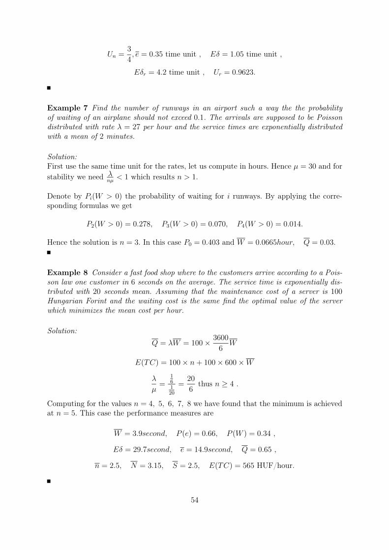
Un =3
4, e = 0.35 time unit , Eδ = 1.05 time unit ,
Eδr = 4.2 time unit , Ur = 0.9623.
Example 7 Find the number of runways in an airport such a way the the probabilityof waiting of an airplane should not exceed 0.1. The arrivals are supposed to be Poissondistributed with rate λ = 27 per hour and the service times are exponentially distributedwith a mean of 2 minutes.
Solution:First use the same time unit for the rates, let us compute in hours. Hence µ = 30 and forstability we need λ
nµ< 1 which results n > 1.
Denote by Pi(W > 0) the probability of waiting for i runways. By applying the corre-sponding formulas we get
P2(W > 0) = 0.278, P3(W > 0) = 0.070, P4(W > 0) = 0.014.
Hence the solution is n = 3. In this case P0 = 0.403 and W = 0.0665hour, Q = 0.03.
Example 8 Consider a fast food shop where to the customers arrive according to a Pois-son law one customer in 6 seconds on the average. The service time is exponentially dis-tributed with 20 seconds mean. Assuming that the maintenance cost of a server is 100Hungarian Forint and the waiting cost is the same find the optimal value of the serverwhich minimizes the mean cost per hour.
Solution:Q = λW = 100× 3600
6W
E(TC) = 100× n+ 100× 600×W
λ
µ=
16120
=20
6thus n ≥ 4 .
Computing for the values n = 4, 5, 6, 7, 8 we have found that the minimum is achievedat n = 5. This case the performance measures are
W = 3.9second, P (e) = 0.66, P (W ) = 0.34 ,
Eδ = 29.7second, e = 14.9second, Q = 0.65 ,
n = 2.5, N = 3.15, S = 2.5, E(TC) = 565 HUF/hour.
54
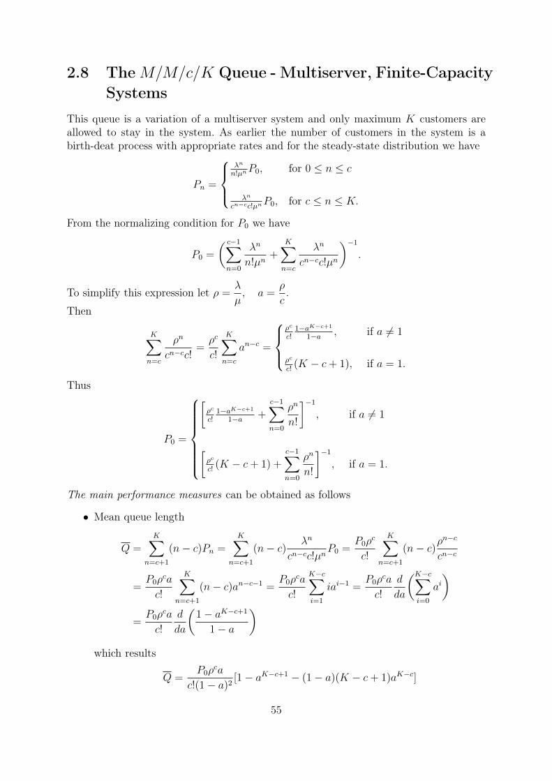
2.8 TheM/M/c/K Queue - Multiserver, Finite-CapacitySystems
This queue is a variation of a multiserver system and only maximum K customers areallowed to stay in the system. As earlier the number of customers in the system is abirth-deat process with appropriate rates and for the steady-state distribution we have
Pn =
λn
n!µnP0, for 0 ≤ n ≤ c
λn
cn−cc!µnP0, for c ≤ n ≤ K.
From the normalizing condition for P0 we have
P0 =
( c−1∑n=0
λn
n!µn+
K∑n=c
λn
cn−cc!µn
)−1
.
To simplify this expression let ρ =λ
µ, a =
ρ
c.
Then
K∑n=c
ρn
cn−cc!=ρc
c!
K∑n=c
an−c =
ρc
c!1−aK−c+1
1−a , if a 6= 1
ρc
c!(K − c+ 1), if a = 1.
Thus
P0 =
[ρc
c!1−aK−c+1
1−a +c−1∑n=0
ρn
n!
]−1
, if a 6= 1
[ρc
c!(K − c+ 1) +
c−1∑n=0
ρn
n!
]−1
, if a = 1.
The main performance measures can be obtained as follows
• Mean queue length
Q =K∑
n=c+1
(n− c)Pn =K∑
n=c+1
(n− c) λn
cn−cc!µnP0 =
P0ρc
c!
K∑n=c+1
(n− c)ρn−c
cn−c
=P0ρ
ca
c!
K∑n=c+1
(n− c)an−c−1 =P0ρ
ca
c!
K−c∑i=1
iai−1 =P0ρ
ca
c!
d
da
(K−c∑i=0
ai)
=P0ρ
ca
c!
d
da
(1− aK−c+1
1− a
)which results
Q =P0ρ
ca
c!(1− a)2[1− aK−c+1 − (1− a)(K − c+ 1)aK−c]
55

In particular, if a = 1 then the L’Hopital’s rule should be applied twice.
• Mean number of customers in the systemIt is easy to see that
λ = λ(1− PK) = µc
and sinceN = Q+ c
we getN = Q+ ρ(1− PK).
• Mean response and waiting timesThe mean times can be obtained by applying the Little’s law, that is
T =N
λ(1− PK)
W =Q
λ(1− PK)
In the case of an M/M/1/K system these formulas are simplified to
P0 =
{1−a
1−aK+1 , (a 6= 1)1
K+1, (a = 1)
Pn =
{(1−a)an
1−aK+1 , (a 6= 1)1
K+1, (a = 1)
Q =
{a
1−a −a(KaK+1)
1−aK+1 , (a 6= 1)K(K−1)2(K+1)
, (a = 1)
N = Q+ (1− P0).
• Distribution at the arrival instantsBy applying the Bayes’s rule we have
Πn ≡ P ( there are n customers in the system| a customer is about to enter into the system )
= lim∆t→0
{[λ∆t+ o(∆t)]Pn∑K−1n=0 [λ∆t+ o(∆t)]Pn
}= lim
∆t→0
{[λ+ o(∆t)/∆t]Pn∑K−1n=0 [λ+ o(∆t)/∆t]Pn
}=
λPn
λ∑K−1
n=0 Pn=
Pn1− PK
, (n ≤ K − 1).
Obviously in the case of an M/M/c/∞ system Πn = Pn since PK tends to 0.
56
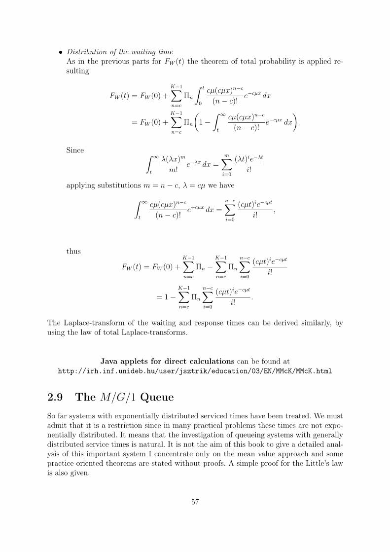
• Distribution of the waiting timeAs in the previous parts for FW (t) the theorem of total probability is applied re-sulting
FW (t) = FW (0) +K−1∑n=c
Πn
∫ t
0
cµ(cµx)n−c
(n− c)!e−cµx dx
= FW (0) +K−1∑n=c
Πn
(1−
∫ ∞t
cµ(cµx)n−c
(n− c)!e−cµx dx
).
Since ∫ ∞t
λ(λx)m
m!e−λx dx =
m∑i=0
(λt)ie−λt
i!
applying substitutions m = n− c, λ = cµ we have∫ ∞t
cµ(cµx)n−c
(n− c)!e−cµx dx =
n−c∑i=0
(cµt)ie−cµt
i!,
thus
FW (t) = FW (0) +K−1∑n=c
Πn −K−1∑n=c
Πn
n−c∑i=0
(cµt)ie−cµt
i!
= 1−K−1∑n=c
Πn
n−c∑i=0
(cµt)ie−cµt
i!.
The Laplace-transform of the waiting and response times can be derived similarly, byusing the law of total Laplace-transforms.
Java applets for direct calculations can be found athttp://irh.inf.unideb.hu/user/jsztrik/education/03/EN/MMcK/MMcK.html
2.9 The M/G/1 Queue
So far systems with exponentially distributed serviced times have been treated. We mustadmit that it is a restriction since in many practical problems these times are not expo-nentially distributed. It means that the investigation of queueing systems with generallydistributed service times is natural. It is not the aim of this book to give a detailed anal-ysis of this important system I concentrate only on the mean value approach and somepractice oriented theorems are stated without proofs. A simple proof for the Little’s lawis also given.
57

Little’s Law
As a first step for the investigations let us give a simple proof for the Little’s theorem,Little’s law, Little’s formula, which states a relation between the mean number ofcustomers in the systems, mean arrival rate and the mean response time. Similar versioncan be stated for the mean queue length, mean arrival rate and mean waiting time.
Let α(t) denote the number of customers arrived into the system in a time interval (0, t),and let δ(t) denote the number of departed customers in (0, t). Supposing that N(0) = 0,the number of customert in the system at time t is N(t) = α(t)− δ(t).Let the mean arrival rate into the system during (0, t) be defined as
λ̄t :=α(t)
t.
Let γ(t) denote the overall sojourn times of the customers until t and let T t be definedas the mean sojourn time for a request. Clearly
T t =γ(t)
α(t).
Finally, let N̄t denote the mean number of customers in the system during in the interval(0, t), that is
N̄t =γ(t)
t.
From these relations we haveN̄t = λ̄tT̄t.
Supposing that the following limits exist
λ̄ = limt→∞
λ̄t, T̄ = limt→∞
T̄t.
we getN̄ = λ̄T̄ ,
which is called Little’s law .
Similar version isQ̄ = λ̄W̄ .
The Embedded Markov Chain
As before let N(t) denote the number of customers in the system at time t. As timeevolves the state changes and we can see that changes to neighboring states occur, upand down, that is from state k either to k + 1 or to k − 1. Since we have a single serverthe number of k → k + 1 type transitions may differ by at most one from the number ofk + 1→ k type transitions. So if the system operate for a long time the relative frequen-cies should be the same. It means that in stationary case the distributions at the arrivalinstants and the departure instants should be the same. More formally, Πk = Dk.
58

For further purposes we need the following statementsStatement 1 For Poisson arrivals
P (N (t) = k) = P (an arrival at time t finds k customers in the system ) .
Statement 2 If in any system N (t) changes its states by one then if either one of thefollowing limiting distribution exists, so does the other and they are equal.
Πk := limt→∞
(an arrival at time t finds k customers in the system ) ,
Dk := limt→∞
(a departure at time t leaves k customers behind ) ,
Πk = Dk.
Thus for an M/G/1 systemΠk = Pk = Dk,
that is in stationary case these 3 types of distributions are the same.
Due to their importance we prove them. Les us consider first Statement 1.Introduce the following notation
Pk(t) := P (N (t) = k) ,
Πk(t) := P (an arriving customer at instant t finds k customers in the system ) .
Let A(t, t+ ∆t) be the event that one arrival occurs in the interval (t, t+ ∆t). Then
Πk(t) = lim∆t→0
P (N (t) = k | A(t, t+ ∆t)) .
By the definition of the conditional probability we have
Πk(t) = lim∆t→0
P (N (t) = k,A(t, t+ ∆t))
P (A(t, t+ ∆t))=
= lim∆t→0
P (A(t, t+ ∆t) | N (t) = k)P (N(t) = k)
P (A(t, t+ ∆t)).
Due to the memoryless property of the exponential distribution event A(t, t + ∆t) doesnot depend on the number of customers in the systems and even on t itself thus
P (A(t, t+ ∆t) | N (t) = k) = P (A(t, t+ ∆t)) ,
henceΠk(t) = lim
∆t→0P (N(t) = k) ,
that isΠk(t) = Pk(t).
This holds for the limiting distribution as well, namely
Πk = limt→∞
Πk(t) = limt→∞
Pk(t) = Pk.
59

Let us prove Statement 2 by the help of Statement 1 .
Let R̂k (t) denote the number of arrivals into the system when it is in state k during thetime interval (0, t) and let D̂k (t) denote the number of departures that leave the systembehind in state k during (0, t). Clearly
(2.9) |R̂k (t)− D̂k (t) | ≤ 1.
Furthermore if the total number of departures is denoted by D (t), and the total numberof arrivals is denoted by R (t) then
D (t) = R (t) +N (0)−N (t) .
The distribution at the departure instants can be written as
Dk = limt→∞
D̂k (t)
D (t).
It is easy to see that the after simple algebra we have
D̂k (t)
D (t)=R̂k (t) + D̂k (t)− R̂k (t)
R (t) +N (0)−N (t).
Since N (0) is finite and N (t) is also finite due to the stationarity from (2.9) and R̂ (t)→∞, with probability one follows that
Dk = limt→∞
D̂k (t)
D (t)= lim
t→∞
R̂k (t)
R (t)= Πk.
Consequently, by using Statement 1 the equality of the three probabilities follows.
Mean Value Approach
Let S denote the service time and let R denote the residual ( remaining) service time.Then it can easily be seen that
E(W ) =∞∑k=1
(E(R) + (k − 1)E(S)) Πk
=∞∑k=1
E(R)Pk +
(∞∑k=1
(k − 1)Pk
)E(S) = E(R)ρ+ E(Q)E(S),
where E(R) denotes the mean residual time.By applying the Little’s law we have
E(Q) = λE(W ),
and thus
(2.10) E(W ) =ρE(R)
1− ρ
60
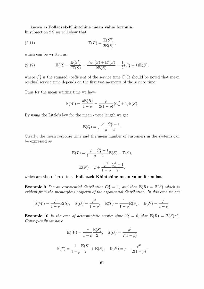
known as Pollaczek-Khintchine mean value formula.In subsection 2.9 we will show that
(2.11) E(R) =E(S2)
2E(S),
which can be written as
(2.12) E(R) =E(S2)
2E(S)=V ar(S) + E2(S)
2E(S)=
1
2(C2
S + 1)E(S),
where C2S is the squared coefficient of the service time S. It should be noted that mean
residual service time depends on the first two moments of the service time.
Thus for the mean waiting time we have
E(W ) =ρE(R)
1− ρ=
ρ
2(1− ρ)(C2
S + 1)E(S).
By using the Little’s law for the mean queue length we get
E(Q) =ρ2
1− ρC2S + 1
2.
Clearly, the mean response time and the mean number of customers in the systems canbe expressed as
E(T ) =ρ
1− ρC2S + 1
2E(S) + E(S),
E(N) = ρ+ρ2
1− ρC2S + 1
2,
which are also referred to as Pollaczek-Khintchine mean value formulas.
Example 9 For an exponential distribution C2S = 1, and thus E(R) = E(S) which is
evident from the memoryless property of the exponential distribution. In this case we get
E(W ) =ρ
1− ρE(S), E(Q) =
ρ2
1− ρ, E(T ) =
1
1− ρE(S), E(N) =
ρ
1− ρ.
Example 10 In the case of deterministic service time C2S = 0, thus E(R) = E(S)/2.
Consequently we have
E(W ) =ρ
1− ρE(S)
2, E(Q) =
ρ2
2(1− ρ)
E(T ) =1
1− ρE(S)
2+ E(S), E(N) = ρ+
ρ2
2(1− ρ).
61

For an M/G/1 system we have proved that
Πk = Dk = Pk, k = 0, 1, . . .
therefore the generating function of the number of customers in the system is equal to thegenerating function of the number of customers at departure instant. Furthermore, it isclear that the number of customers at departure instants is equal the number customersarrived during the response time. In summary we have
Dk = Pk =
∞∫0
(λx)k
k!e−λxfT (x)dx.
Thus the corresponding generating function can be obtained as
GN(z) =∞∑k=0
zk∞∫
0
(λx)k
k!e−λxfT (x)dx
=
∞∫0
∞∑k=0
(λxz)k
k!e−λxfT (x)dx
=
∞∫0
e−λ(1−z)xfT (x)dx = LT (λ(1− z)),
that is it can be expressed by the help of the Laplace-transform of the response time T .By applying the properties of the generating function and the Laplace-transform we have
G(k)N (1) = E(N(N − 1) . . . (N(−k + 1))) = (−1)kL
(k)T (0)λk = λkE(T k).
In particular, the first derivative results to the Little’s law, that is
N = λT ,
and hence this formula can be considered as the generalization of the Little’s law for anM/G/1 queueing systems.By the help of this relation the higher moments of N can be obtained, thus the variancecan be calculated if the second moment of T is known.
Residual Service Time
Let us suppose that the tagged customer arrives when the server is busy and denote thetotal service time of the request in service by X, that is a special interval. Let fX(x)denote the density function of X. The key observation to find fX(x) is that it is morelikely that the tagged customer arrives in a longer service time than in a short one. Thusthe probability that X is of length x should be proportional to the length x as well asthe frequency of such service times, which is fS(x) dx. Thus we may write
P (x ≤ X ≤ x+ dx) = fX(x)dx = CxfS(x)dx,
62

where C is a constant to normalize this density. That is
C−1 =
∫ ∞x=0
xfS(x)dx = E(S),
thusfX(x) =
xfS(x)
E(S).
E(X) =
∫ ∞0
xfX(x) dx =1
E(S)
∫ ∞0
x2fS(x) dx =E(S2)
E(S).
Since the tagged customers arrives randomly in service time S hence the mean residualcan be obtained as
E(R) =E(X)
2=
E(S2)
2E(S)
Example 11 Let the service time be Erlang distributed with parameters (n, µ) then
E(S) =n
µ, V ar(S) =
n
µ2,
thusE(S2) = V ar(S) + E2(S) =
n(1 + n)
µ2
henceE(R) =
1 + n
2µ.
It is easy to see that using this approach the the density function the residual servicetime can be calculated. Given that the tagged customer arrives in a service time of lengthx, the arrival moment will be a random point within this service time, that is it will beuniformly distributed within the service time interval (0, x). Thus we have
P (x ≤ X ≤ x+ dx, y ≤ R ≤ y + dy) =dy
xfX(x)dx, qquad0 ≤ y ≤ x.
After substitution for fX(x) and integrating over x we get the desired density functionof the residual service time, that is
fR(y) =1− FS(y)
E(S).
Hence
E(R) =
∞∫0
xfR(x)dx =
∞∫0
x1− FS(x)
E(S)dx,
ThusE(R) =
E(S2)
2E(S).
63

Now let us show how to calculate this type of integrals.Let X be a nonnegative random variable with finite nth moment. Then
∞∫0
xnf(x)dx =
y∫0
xnf(x)dx+
∞∫y
xnf(x)dx,
thus∞∫y
xnf(x)dx =
∞∫0
xnf(x)dx−y∫
0
xnf(x)dx.
Since∞∫y
xnf(x)dx ≥ yn∞∫y
f(x)dx = yn (1− F (y)) ,
hence
0 ≤ yn (1− F (y)) ≤∞∫
0
xnf(x)dx−y∫
0
xnf(x)dx,
therefore
0 ≤ limy→∞
yn (1− F (y)) ≤∞∫
0
xnf(x)dx− limy→∞
y∫0
xnf(x)dx,
that islimy→∞
yn (1− F (y)) = 0.
After these using integration by parts keeping in mind the above relation we get
∞∫0
xn−1(1− F (x))dx =
∞∫0
xn
nf(x)dx =
E(Xn)
n.
In particular, for n = 2 we obtain
E(R) =E(S2)
2E(S)
Pollaczek-Khintchine and Takács formulas
The following relations are commonly referred to as Pollaczek-Khintchine transformequations
GN(z) = LS(λ− λz)(1− ρ)(1− z)
LS(λ− λz)− z,
LT (t) = LS(t)t(1− ρ)
t− λ+ λLS(t),
LW (t) =t(1− ρ)
t− λ+ λLS(t),
64

by the help of which, in principle, the distribution of the number of customers in the sys-tem, the density function of the response and waiting times can be obtained. Of coursethis time we must be able to invert the involved Laplace-transforms.
Takács Recurrence Theorem
E(W k) =λ
1− ρ
k∑i=1
(k
i
)E(Si+1)
i+ 1E(W k−i)
that is moments of the waiting time can be obtained in terms of lower moments of thewaiting time and moments of the service time. It should be noted to get the kth momentof W the k + 1th moment of the service time should exist.
Since W ,S are independent and T = W + S the kth moment of the response time canalso be computed by
E(T k) =k∑l=0
(n
l
)E(W l) · E(Sk−l).
By using these formulas the following relations can be proved
E(W ) =λE(S2)
2(1− ρ)=ρE(S)
1− ρ
(1 + C2
S
2
),
E(T ) = E(W ) + E(S),
E(W 2) = 2(W )2 +λE(S3)
3(1− ρ),
E(T 2) = E(W 2) +E(S2)
1− ρ,
V ar(W ) = E(W 2)− (E(W ))2,
V ar(T ) = V ar(W + S) = V ar(W ) + V ar(S).
Since
E(N(N − 1)) = λ2E(T 2)
after elementary but lengthly calculation we have
V ar(N) =λE(S3)
3(1− ρ)+
(λE(S2)
2(1− ρ)
)2
+λ(3− 2ρ)E(S2)
2(1− ρ)+ ρ(1− ρ).
Since
E(Q2) =∞∑k=1
(k − 1)2Pk =∞∑k=1
k2Pk − 2∞∑k=1
kPk +∞∑k=1
Pk
= E(N2)− 2N + ρ
65
by elementary computations we can prove that
V ar(Q) =λE(S3)
3(1− ρ)+
(λE(S2)
2(1− ρ)
)2
+λE(S2)
2(1− ρ).
Now let us turn our attention to the Laplace-transform of the busy period of the server.
Lajos Takács proved that
Lδ(t) = LS(t+ λ− λLδ(t)),
that is for the Laplace-transform Lδ(t) a function equation should be solved ( which isusually impossible to invert ).However, by applying this equation the moments the busy period can be calculated.
First determine E(δ). Using the properties of the Laplace-transform we have
L′δ(0) = (1− λL′δ(0))L′S(0)
E(δ) = (1 + λE(δ))E(S)
E(δ) =E(S)
1− ρ=
1
λ
ρ
1− ρ
which was obtained earlier by the well-known relation
E(δ)1λ
+ E(δ)= ρ.
After elementary but lengthly calculations it can be proved that
V ar(δ) =V ar(S) + ρ(E(S))2
(1− ρ)3.
Now let us consider the generating function of the customers served during a busy period.It can be proved that
GNd(δ)(z) = zLS(λ− λGNd(δ)(z))
which is again a functional equation but using derivations the higher moments can becomputed.Thus for the mean numbers we have
E(Nd(δ)) = 1 + λE(S)E(Nd(δ))
E(Nd(δ)) =1
1− ρ,
66
which can also be obtained by relation
E(δ) = E(S)E(Nd(δ))
since
1
λ
ρ
1− ρ= E(S) · E(Nd(δ))
E(Nd(δ)) =ρ
ρ(1− ρ)=
1
1− ρ.
It can be proved that
V ar(Nd(δ)) =ρ(1− ρ) + λ2E(S2)
(1− ρ)3.
It is interesting to note that the computation of V ar(δ), V ar(Nd(δ)) does not require theexistence of E(S3), as it in the case of V ar(N), V ar(Q), V ar(T ), V ar(W ).
As it is one of the most widely used queueing system the calculation of the main perfor-mance measure is of great importance. Tis can be done by the help of our Java applets
Java applets for direct calculations can be found at
http://irh.inf.unideb.hu/user/jsztrik/education/03/EN/MH21/MH21.html
http://irh.inf.unideb.hu/user/jsztrik/education/03/EN/MGamma1/MGamma1.html
http://irh.inf.unideb.hu/user/jsztrik/education/03/EN/MEk1/MEk1.html
http://irh.inf.unideb.hu/user/jsztrik/education/03/EN/MD1/MD1.html
67

68

Chapter 3
Finite-Source Systems
So far we have been dealing with such queueing systems where arrivals followed a Poissonprocess, that is the source of customers is infinite. In this chapter we are focusing onthe finite-source population models. They are also very important from practical pointof view since in many situation the source is finite. Let us investigate the example of theso-called machine interference problem treated by many experts.
Let us consider n machines that operates independently of each other. The operationtimes and service times are supposed to be independent random variables with givendistribution function. After failure the broken machines are repaired by a single or multi-ple repairmen according to a certain discipline. Having been repaired the machine startsoperating again and the whole process is repeated.
This simple model has many applications in various fields, for example in manufacturing,computer science, reliability theory, management science, just to mention some of them.For a detailed references on the finite-source models and their application the interestedreader is recommended to visit the following link
http://irh.inf.unideb.hu/user/jsztrik/research/fsqreview.pdf
3.1 The M/M/r/r/n Queue, Engset-Loss System
As we can see depending on the system capacity r in an M/M/r/r/n a customer mayfind the system full. Despite of the infinite-source model where the customer is lost, inthe finite-source model this request returns to the source and stay there for a exponen-tially distributed time. Since all the random variables are supposed to be exponentiallydistributed the number of customers in the system is a birth-death process with thefollowing rates
λk = (n− k)λ , 0 ≤ k < r,
µk = kµ , 1 ≤ k ≤ r,
69
hence the distribution can be obtained as
Pk =
(n
k
)ρkP0, 0 ≤ k ≤ r,
Pk =
(n
k
)ρk
r∑i=0
(n
i
)ρi,
which is called a truncated binomial or Engset distribution .This is the distribution of a finite-source loss or Engset system .Specially, if r = n that is no loss and each customer has its own server the distributionhas a very nice form, namely
Pk =
(n
k
)ρk
n∑i=0
(n
i
)ρi
=
(n
k
)ρk
(1 + ρ)n
=
(n
k
)(ρ
1 + ρ
)k (1− ρ
1 + ρ
)n−k,
that is we have a binomial distribution with success parameter ip =ρ
1 + ρ.
That is p is the probability that a given request is in the system. It is easy to see thatthis distribution remains valid even for a G/G/n/n/n system since
p =E(S)
E(S) + E(τ)=
ρ
1 + ρ,
where ρ = E(S)E(τ)
, and E(τ) denotes the mean time a customer spends in the source.
As before it is easy to see that the performance measures are as follows
• Mean number of customers in the system N
N =r∑
k=0
kPk, r = N, US =r
r=N
r,
• Mean number of customers in the source m
m = n−N
• Utilization of a source Ut
Ut =m
n=
E(τ)
E(τ) + 1µ
,
70
thus
E(τ) =1
µ
Ut1− Ut
.
This help us to calculate the mean number of retrials of a customer from the sourceto enter to the system. That it we have
E(NR) = λE(τ),
hence the mean number of rejection is E(NR)− 1.
The blocking probability, that is the probability that a customer find the system full athis arrival, by the help of the Bayes’s theorem can be calculated as
PB(n, r) =(n− r)Pr(n, r)r∑i=0
(n− i)Pk(n, r)= Pr(n− 1, r).
This can easily be verified by
PB(n, r) = limh→0
((n− r)λh+ o(h))Pr(n, r)r∑i=0
((n− i)λh+ o(h))Pi(n, r)
=(n− r)Pr(n, r)r∑i=0
(n− i)Pi(n, r)
=
(n− r)(n
r
)ρr
r∑i=0
(n− i)(n
i
)ρi
=(n− r) n!
r!(n−r)!ρr
r∑i=0
(n− i) n!
i!(n− i)!ρi
=
(n−1)!r!(n−1−r)!ρ
r
r∑i=0
(n− 1)!
i!(n− 1− i)!ρi
=
(n− 1
r
)ρr
r∑i=0
(n− 1
i
)ρi
= Pr(n− 1, r).
Let E(n, r, ρ) denote the blocking probability, that is E(n, r, ρ) = Pr(n − 1, r), which iscalled Engset’s loss formula.In the following we show a recursion for this formula, namely
E(n, r, ρ) =
(n− 1
r
)ρr
r∑i=0
(n− 1
i
)ρi
=
(n− 1
r − 1
)n−rrρr
r−1∑i=0
(n− 1
i
)ρi +
(n− 1
r − 1
)n− rr
ρr
=n−rrρE(n, r − 1, ρ)
1 + n−rrρE(n, r − 1, ρ)
=(n− r)ρE(n, r − 1, ρ)
r + (n− r)ρE(n, r − 1, ρ).
71
The initial value is
E(n, 1, ρ) = P1(n− 1, 1) =(n− 1)ρ
1 + (n− 1)ρ.
It is clear that
limn→∞, λ→0, nλ→λ′
E(n, r, ρ) = B(n, ρ′),
where
ρ′ =λ′
µ
which van be seen formally, too. Moreover, as (n− r)ρ→ ρ′ the well-known recursion forB(n, ρ′) is obtained which also justifies the correctness of the recursion for E(n, r, ρ).
In particular, if r = n then it is easy to see that N = n ρ1+ρ
and thus
US =ρ
1 + ρ, m =
n
1 + ρ, Ut =
1
1 + ρ, E(τ) =
1
λ, E(NR) = 1, PB = 0,
which was expected.
In general case
µ = rµ = λ =r−1∑k=0
λ(n− k)Pk 6= λ(n−N), T =1
µ.
Let us consider the distribution of the system at the instant when an arriving customerenters into the system.By using the Bayes’s law we have
Πk = limh→0
(λkh+ o(h))Pkr−1∑i=0
(λih+ o(h))Pi
=λkPk
r−1∑i=0
λiPi
, k = 0, · · · , r − 1
T =1
µ
r−1∑k=0
λkPkr−1∑i=0
λiPi
=1
µ
λ · T = µr · 1
µ= r = N
which Little’s formula for the finite-source loss system.
72
3.2 The M/M/1/n/n QueueIt is the traditional machine interference problem, where the broken machines has towait and the single repairman fixes the failed machine in FIFO order. Assume the theoperating times are exponentially distributed with parameter λ and the repair rate is µ.All random variables are supposed to be independent of each other.
Let N(t) denote the number of customers in the system at time t, which is a birth-deathprocess with birth rates
λk =
(n− k)λ , ha 0 ≤ k ≤ n,
0 , ha k > n,
and with death rateµk = µ, k ≥ 1.
Thus for the distribution we have
Pk =n!
(n− k)!%kP0 = (n− k + 1)%Pk−1,
where
% =λ
µ,
andP0 =
1
1 +n∑k=1
n!(n−k)!
%k=
1n∑k=0
n!(n−k)!
%k.
Since the state space is finite the steady-state distribution always exists but if % > 1 thenmore repairmen is needed.
For numerical calculation other forms are preferred that is why we introduce some nota-tions.Let P (k;λ) a λ denote the Poisson distribution with parameter λ) and let Q(k;λ) denoteits cumulative distribution function, that is
P (k;λ) =λk
k!e−λ, 0 ≤ k <∞;
Q(k;λ) =k∑i=0
P (i;λ), 0 ≤ k <∞.
First we show thatPk =
P (n− k;R)
Q(n;R), 0 ≤ k ≤ n,
73

whereR =
µ
λ= %−1.
By elementary calculations we have
P (n− k;R)
Q(n;R)=
n!(n−k)!
(µλ
)n−ke−
µλ
n∑i=0
n!i!
(µλ
)ie−
µλ
=
n!(n−k)!
(λµ
)kn∑i=0
n!i!
(λµ
)n−i =
n!(n−k)!
(λµ
)k∑n
k=0n!
(n−i)!
(λµ
)i = Pk.
Hence a very important consequence is
P0 = B(n,R).
The main performance measures can be obtained as follows
• Utilization of the server and the throughput of the systemFor the utilization of the server we have
Us = 1− P0 = 1−B(n,R).
By using the cumulative distribution function this cab be written as
Us =Q(n− 1;R)
Q(n;R).
For the throughput of the system we obtain
λt = µUs.
• Mean number of customers in the system N can be calculated as
N =n∑k=0
kPk = n−n∑k=0
(n− k)Pk =
= n− 1
%
n∑k=0
(n− k)%Pk = n− 1
%
n−1∑k=0
Pk+1 =
= n− 1
%(1− P0) = n− Us
%.
In other form
N = n− RQ(n− 1;R)
Q(n;R)= n− Us
%.
74
• Mean queue length, mean number of customers waiting can be derived as
Q =n∑k=1
(k − 1)Pk =n∑k=1
kPk −n∑k=1
Pk = n− µ
λ(1− P0)− (1− P0) =
= n− (1− P0)(1 +µ
λ) = n−
(1 +
1
%
)Us.
• Mean number of customers in the source can be calculated as
m =n∑k=0
(n− k)Pk = n−N =µ
λ(1− P0) =
Us%.
• Mean busy period of the serverSince
Us = 1− P0 =Eδ
1nλ
+ Eδ,
thusEδ =
1− P0
nλP0
=Us
nλ(1− Us).
In computer science and reliability theory application we often need the followingmeasure
• Utilization of a given source ( machine, terminal )The utilization of the ith source is defined by
U (i) = limT→∞
1
T
T∫0
χ(at time t the ith source is active)dt
ThenU (i) = P ( there is a request in the ith source) .
Hence the overall utilization of the sources is
Un =n∑k=0
(n− k)Pk = m =µ
λ(1− P0).
Thus the utilization of any source is
Ut =µ
nλ(1− P0) =
m
n.
This can be obtained in the following way as well,
U (i) =n∑k=1
n− kn
Pk =m
n,
since the source are homogeneous we have
Ut = U (i) .
75

• Mean waiting timeBy using the result of Tomkó 1 we have
Ut =1/λ
1/λ+W + 1/µ=m
n.
Thusλm =
n
1/λ+W + 1/µ,
andλmW = n−m
(1 +
λ
µ
)= n− Us
%(1 + %) = Q,
which the Litle’s law for the mean waiting time. Hence
W =Q
λm=
1
µ
(n
Us− 1 + %
%
).
The mean response can be obtained as
T = W +1
µ=
1
µ
(n
1− P0
− 1
%
)=
1
µ
(n
Us− 1
%
).
It is easy to prove thatmλT = N,
which is the Little’s law for the mean response time. Clearly we have
mλ
(W +
1
µ
)= Q+m% =
= n− Us%
(1 + %) + Us = n− Us%
= N .
• Further relationsUs = 1− P0 = n%Ut = m%,
and thusmλ = µUs = λt .
It should be noted that the utilization of the server plays a key role in the calculation ofall the main performance measures.
Distribution at the arrival instants
In the following we find the steady-state distribution of the system at arrival instants andin contrary to the infinity-source model is not he same as the distribution at a randompoint. To show this use the Bayes’s theorem, that is
Πk(n) = limh→0
(λkh+ o(h))Pk∑n−1j=0 (λjh+ o(h))Pj
=λkPk∑n−1j=0 λjPj
=
n(n−1)···(n−k)λk
µ1···µkP0∑n−1
j=0n(n−1)···(n−j)λj
µ1···µj P0
=
(n−1)···(n−k)λk
µ1···µk
1 +∑n−1
j=1(n−1)···(n−j)λj
µ1···µj
=
(n−1)···(n−1−k+1)λk
µ1···µk
1 +∑n−1
i=1(n−1)···(n−1−i+1)λi
µ1···µi
= Pk(n− 1)
76
irrespective to the number of servers. It should be noted that this relation shows a veryimportant result, namely that at arrivals the distribution of the system containing nsources is not he same as its distribution at random points, but equals to the randompoint distribution of a system with n− 1 sources.
Distribution at the departure instants
We are interested in the distribution of the number of customers a departing customerleaves behind in the system. This calculations are independent of the number of servers.By applying the Bayes’s theorem we have
Dk(n) = limh→0
(µk+1h+ o(h))Pk+1∑nj=1(µjh+ o(h))Pj
=µk+1Pk+1∑nj=1 µjPj
=
µk+1n(n−1)···(n−k)λk+1
µ1···µk+1P0∑n
j=1µjn(n−1)···(n−j+1)λj
µ1···µj P0
=
(n−1)···(n−k)λk
µ1···µk
1 +∑n
j=2(n−1)···(n−j+1)λj−1
µ1···µj−1
=
(n−1)···(n−1−k+1)λk
µ1···µk
1 +∑n−1
i=1(n−1)···(n−1−i+1)λi
µ1···µi
= Pk(n− 1)
in the case when there is customer left in the system
D0(n) =1
1 +∑n−1
i=1(n−1)···(n−1−i+1)λi
µ1···µi
= P0(n− 1)
if the system becomes empty.
Recursive Relations
Similarly to the previous arguments it is easy to see that the density function of theresponse time can be obtained as
fT (x) =n−1∑k=0
fT (x|k)Πk(n) =n−1∑k=0
µ(µx)k
k!e−µxPk(n− 1).
Hence the mean value is
T (n) =n−1∑k=0
k + 1
µPk(n− 1) =
1
µ(N(n− 1) + 1).
Similarly, for the waiting time we have
fW (x) =n−1∑k=0
fW (x|k)Πk(n) =n−1∑k=0
µ(µx)k−1
(k − 1)!e−µxPk(n− 1),
thus its mean is
W (n) =n−1∑k=0
k
µPk(n− 1) =
1
µ(N(n− 1)),
77
which is clear.We want to verify the correctness of the formula
T (n) =1
µ(N(n− 1) + 1).
As we have shown earlier the utilization can be expressed by the Erlang’s loss formula,hence
N(n) = n−1−B(n, 1
%)
%.
Using the well-known recursive relation we have
B(n,1
%) =
1%B(n− 1, 1
%)
n+ 1%B(n− 1, 1
%)
=B(n− 1, 1
%)
n%+B(n− 1, 1%.
).
Since
N(n− 1) = n− 1−1−B(n− 1, 1
%)
%
thus
%N(n− 1) = (n− 1)%− 1−B(n− 1,
1
%
)B
(n− 1,
1
%
)= 1 + %N(n− 1)− (n− 1)%.
After substitution we have
B
(n,
1
%
)=
1%(1 + %N(n− 1)− (n− 1)%)
n+ 1%(1 + %N(n− 1)− (n− 1)%)
=1 + %N(n− 1)− (n− 1)%
n%+ 1 + %N(n− 1)− (n− 1)%=
1 + %N(n− 1)− (n− 1)%
1 + %N(n− 1) + %.
Therefore
N(n) =n%− 1 +B(n, 1
%)
%=n%− 1 + 1+%N(n−1)−(n−1)%
1+%N(n−1)+%
%
=n%− n%
1+%N(n−1)+%
%= n− n
1 + %N(n− 1) + %.
Fnally
n−N(n) =n
1 + %N(n− 1) + %
1 + %(N(n− 1) + 1) =n
n−N(n)
%(N(n− 1) + 1) =N(n)
n−N(n),
78
which is a recursion for the mean number of customers in the system.
Now we able to prove our relation regarding the mean response time. Keeping in mindthe recursive relation for N(n− 1) we get
T (n) =1
µ(N(n− 1) + 1)
λT (n) = %(N(n− 1) + 1) =N(n)
n−N(n)
λ(n−N(n))T (n) = N(n),
which was proved earlier.
Now let us show how we can verify T (n) directly. It can easily be seen that
US(n) = 1−B(n,1
%) = 1−
1%B(n− 1, )
n+ 1%B(n− 1, 1
%)
=n
n+ 1%B(n− 1, 1
%)
=n%
n%+B(n− 1, 1%)
=n%
n%+ 1− US(n− 1),
that is there is a recursion for the utilization as well. It is also very important because byusing this recursion all the main performance measures can be obtained. Thus if λ, µ, n aregiven we can use the recursion for US(n) and finally substitute it into the correspondingformula. Thus
US(n− 1) = n%+ 1− n%
US(n)= 1 + n%
(1− 1
US(n)
).
SinceN(n− 1) = n− 1− US(n− 1)
%,
we proceed
T (n) =1
µ(N(n− 1) + 1) =
1
µ
(n− 1− US(n− 1)
%+ 1
)
=1
µ
(n− US(n− 1)
%
)=
1
µ
(n−
1 + n%(1− 1US(n)
)
%
)=
1
µ
(n
US(n)− 1
%
),
which shows the correctness of the formula.
In the following let us show to compute T (n),W (n), N(n) recursively. As we have seen
T (n) =1
µ(N(n− 1) + 1)
W (n) = T (n)− 1
µ=
1
µN(n− 1),
79
we have to know how N(n) can be expressed in term of T (n).It can be shown very easily, namely
N(n) = λ(n−N(n))T (n) = λnT (n)− λN(n)T (n)
N(n)(1 + λT (n)) = λnT (n)
N(n) =λnT (n)
1 + λT (n).
The initial values are
T (1) =1
µ
N(1) =%
1 + %.
Now the iteration proceeds as
W (n) =1
µN(n− 1)
T (n) =1
µ+W (n)
N(n) =λnT (n)
(1 + λT )(n)
that is we use a double iteration. The main advantage is that only the mean values areneeded. This method is referred to as mean value analysis.
In the previous section we have derived a recursion for US(n) and thus we may expectthat there is direct recursive relation for the other mean values as well since they dependson the utilization. As a next step we find a recursion for the mean number of customersin the source m(n). It si quite easy since
m(n) =Us(n)
ρ=
n
nρ+ 1− Us(n− 1)=
=
n
ρ
n+1
ρ−m(n− 1)
=n
nρ+ 1− ρm(n− 1).
By using this relation for the utilization of the source can be expressed as
Ut(n) =m(n)
n=
n
nρ+ 1− ρm(n− 1)
1
n=
=
1
n− 1nρ+ 1
n− 1− ρUt(n− 1)
=1
nρ+ 1− (n− 1)ρUt(n− 1).
80
For the mean number of customers in the system we have
N(n) = n− Us(n)
ρ=nρ− Us(n)
ρ=
nρ− nρ
nρ+ 1− Us(n− 1)
ρ=
=n2ρ+ n− nUs(n− 1)− 1
nρ+ 1− Us(n− 1)=
n(nρ− Us(n− 1))
nρ+ 1− Us(n− 1).
Since
N(n− 1) = n− 1− Us(n− 1
ρ=nρ− Us(n− 1)
ρ− 1
ρ(N(n− 1) + 1) = nρ− Us(n− 1)
Us(n− 1) = nρ− ρ(N(n− 1) + 1),
thus after substitution we get
N(n) =nρ(N(n− 1) + 1)
1 + ρ(N(n− 1) + 1).
Finally find the recursion for the mean response time . Starting with
T (n) =1
µ
(n
Us(n)− 1
ρ
)using that
T (n− 1) =1
µ
(n− 1
Us(n− 1)− 1
ρ
)µT (n− 1) =
n− 1
Us(n− 1)− 1
ρ
µT (n− 1) +1
ρ=
n− 1
Us(n− 1)
Us(n− 1) =(n− 1)ρ
λT (n− 1) + 1,
substituting into the recursion for Us(n) we obtain
T (n) =1
µ
nρ− Us(n− 1)
ρ=
1
µ
nλT (n− 1) + 1
λT (n− 1) + 1.
Obviously the missing initial values are
m(1) = Ut(1) =1
1 + %.
81
Distribution Function of the Response Time and Waiting Time
This subsection is devoted to one of the major problems in finite-source queueing systems.To find the distribution function of the response and waiting time is not easy. As it isexpected the theorem of total probability should be used.
Let us determine the density function and then the distribution function. As we did manytimes in earlier chapters the law of total probability should be applied for the conditionaldensity functions and the distribution at the arrival instants. So we can write
fT (n, x) =n−1∑k=0
µ(µx)k
k!e−µx
(µλ
)n−1−k
(n−1−k)!e−
µλ
n−1∑i=0
(µλ)i
i!e−
µλ︸ ︷︷ ︸
Q(n−1,µλ
)
= µ(µx+ µ
λ)n−1
(n− 1)!
e−(µx+µλ
)
Q(n− 1, µλ)
=µP (n− 1, µx+ µ
λ)
Q(n− 1, µλ)
.
Similarly for the waiting time
fW (n, x) =n−1∑k=1
µ(µx)k−1
(k − 1)!e−µxPk(n− 1) =
∑n−2i=0 µ
(µx)i
i!e−µx
(µλ
)n−2−i
(n−2−i)! e−µλ
Q(n− 1, µλ)
=µP (n− 2, µx+ µ
λ)
Q(n− 1, µλ)
.
To get the distribution function we have to calculate the integral
FT (n, x) =
∫ x
0
fT (n, t) dt.
Using the substitution y = µt+ µλ, t = (y − µ
λ) 1µ, dt
dy= 1
µ.
Hence
FT (n, x) =
∫ µx+µλ
µλ
yn−1
(n−1)!e−y dy
Q(n− 1, µλ)
=
[1−
∑n−1i=0
yi
y!e−y]µx+µ
λ
µλ
Q(n− 1, µλ)
= 1−Q(n− 1, µx+ µ
λ)
Q(n− 1, µλ)
.
Similarly for the waiting time we have
FW (n, x) = 1−Q(n− 2, µx+ µ
λ)
Q(n− 1, µλ)
.
Now let us determine the distribution function by the help of the conditional distributionfunctions. Clearly we have to know the distribution function of the Erlang distributions,thus we can proceed as
82
FT (x) =n−1∑k=0
(1−
k∑j=0
(µx)j
j!e−µx
)Pk(n− 1)
= 1−n−1∑k=0
( k∑j=0
(µx)j
j!e−µx
)Pk(n− 1)
= 1−n−1∑k=0
Q(k, µx)Pk(n− 1) = 1−n−1∑k=0
Q(k, µx)
(µλ
)n−1−k
(n−1−k)!e−
µλ
Q(n− 1, µλ)
= 1−Q(n− 1, µx+ µ
λ)
Q(n− 1, µλ)
Meantime we have used that
∫ λ
0
tj
j!e−t dt = 1−
j∑i=0
λi
i!e−λ
and thus
l∑j=0
µl−j
(l − j)!e−µ
j∑i=0
λi
i!e−λ
can be written as
l∑j=0
(1−
∫ λ
0
tj
j!e−t dt
)µl−j
(l − j)!e−µ
=l∑
j=0
µl−j
(l − j)!e−µ︸ ︷︷ ︸
Q(l,µ)
−∫ λ
0
(t+ µ)l
l!e−(t+µ) = Q(l, µ)−
∫ λ+µ
µ
yl
l!e−y dy
= Q(l, µ)−[1−
l∑i=0
yi
i!e−y]λ+µ
µ
= Q(l, λ+ µ).
During the calculations we could see that the derivative of Q(k, t) is −P (k, t), which canbe used to find the density function, that is
fT (x) =µP (n− 1, µx+ µ
λ)
Q(n− 1, µλ)
.
83

Generating Function of the Customers in the System
Using the definition the generating function GN(s) can be calculated as
GN(s) =n∑k=0
sk(µλ
)n−k(n− k)!
P0
= snn∑k=0
(1sρ
)n−k(n− k)!
P0
= sne−1ρ(1− 1
s)Q(n, 1
ρs
)Q(n, 1
ρ
) .
This could be derived in the following way. Let denote by F the number of customers inthe source. As we have proved earlier its distribution can be obtained as the distributionof an Erlang loss system with traffic intensity 1
ρ. Since the generating function of this
system has been obtained we can use this fact. Thus
GN(s) = E(sN) = E(sn−F ) = snE(s−F ) = snGF
(1
s
)
= sne−1ρ(1− 1
s)Q(n, 1
ρs
)Q(n, 1
ρ
) .To verify the formula let us compute the mean number of customers in the system. Bythe property of the generating function we have
N(n) = G′N(n)(1) =
(snGF (n)
(1
s
))′s=1
G′N(n)(s) = n · sn−1GF (n)
(1
s
)+ snG′F (n)
(1
s
)(− 1
s2
),
thus
N(n) = nGF (n)(1)−G′F (n)(1) = n− 1
ρ
(1−B
(n,
1
ρ
))= n− US(n)
ρ.
Laplace-transform of the Response Time and Waiting Time
Solution 1
By the law of the total Laplace-transforms we have
LT (s) =n−1∑k=0
(µ
µ+ s
)k+1
Pk(n− 1)
84

since the conditional response time is Erlang distributed with parameters (k + 1, µ).Substituting Pk(n− 1) we get
LT (s) =n−1∑k=0
(µ
µ+ s
)k+1(µλ
)n−1−k
(n− 1− k)!
e−µλ
Q(n− 1, µ
λ
)
=
n−1∑k=0
(µ+sµ
)−k−1
·(µ+sµ
)n· (µλ)
n−1−k
(n−1−k)!e−
µλ(
µ+sµ
)nQ(n− 1, µ
λ
)
=
(µ
µ+ s
)ne−
µλ
n−1∑k=0
(µ+sµ· µλ
)n−1−k· 1
(n−1−k)!
Q(n− 1, µ
λ
)=
(µ
µ+ s
)ne−
µλQ(n− 1, µ+s
λ
)· eµ+sλ
Q(n− 1, µ
λ
)=
(µ
µ+ s
)nesλQ(n− 1, µ+s
λ
)Q(n− 1, µ
λ
) .
Solution 2
Let us calculate LT (s) by the help of the density function. Since the denominator is aconstant we have to determine the Laplace-transform of the numerator, that is
LNum(s) =
∞∫0
µ
(µx+ µ
λ
)n−1
(n− 1)!e−(µx+µ
λ) · e−sxdx
= e−µλ
∞∫0
µ
(µx+ µ
λ
)n−1
(n− 1)!e−(µ+s)xdx.
By using the binomial theorem we get
85
Lsz(s) =e−
µλ
(n− 1)!
∞∫0
µn−1∑k=0
(n− 1
k
)(µx)k
(µλ
)n−1−k· e−(µ+s)xdx
= e−µλ
n−1∑k=0
(µλ
)n−1−k
(n− 1− k)!
∞∫0
µ(µx)k
k!e−(µ+s)xdx
= e−µλ
n−1∑k=0
(µλ
)n−1−k
(n− 1− k)!
(µ
µ+ s
)k+1
= e−µλ
(µ
µ+ s
)n n−1∑k=0
(µλ· µ+s
µ
)n−1−k
(n− 1− k)!
= e−µλ
(µ
µ+ s
)nQ
(n− 1,
µ+ s
λ
)· e
µ+sλ
=
(µ
µ+ s
)nQ
(n− 1,
µ+ s
λ
)· e
sλ .
Since
LT (s) =LNum(s)
Q(n− 1, µ
λ
) ,thus
LT (s) =
(µ
µ+ s
)nesλQ(n− 1, µ+s
λ
)Q(n− 1, µ
λ
) .
Solution 3The Laplace-transform of the numerator be can obtained as
LNum(s) =
∞∫0
µ
(µx+ µ
λ
)n−1
(n− 1)!e−(µx+µ
λ) · e−sxdx
Substituting t = µx+ µλwe get
x =1
µ
(t− µ
λ
),
dx
dt=
1
µ,
86
and thus
LNum(s) =
∞∫µλ
µtn−1
(n− 1)!e−te−
sµ(t−µλ) 1
µdt
= esµ
∞∫µλ
tn−1
(n− 1)!e−(1+ s
µ)t
dt
= esµ
(µ
µ+ s
)n−1∞∫µλ
((1 + s
µ
)t)n−1
(n− 1)!e−(1+ s
µ)t
dt.
Substituting again y = µ+sµt dt
dy= µ
µ+s, thus
LNum(s) = esλ
(µ
µ+ s
)n ∞∫µ+sλ
yn−1
(n− 1)!e−ydy
= esλ
(µ
µ+ s
)n·Q(n− 1,
µ+ s
λ
),
therefore
LT (s) =LNum(s)
Q(n− 1, µ
λ
) = esλ
(µ
µ+ s
)n·Q(n− 1, µ+s
λ
)Q(n− 1, µ
λ
) .
That is all 3 solutions gives the same result. Thus, in principle the higher moments ofthe response time can be evaluated.
Since LT (s) = LW (s) · µµ+s
, thus
LW (s) =
(µ
µ+ s
)n−1
esλQ(n− 1, µ+s
λ
)Q(n− 1, µ
λ
) .
Java applets for direct calculations can be found athttp://irh.inf.unideb.hu/user/jsztrik/education/03/EN/MM1KK/MM1KK.html
http://irh.inf.unideb.hu/user/jsztrik/education/03/EN/MHypo1KK/MHypo1KK.html
87
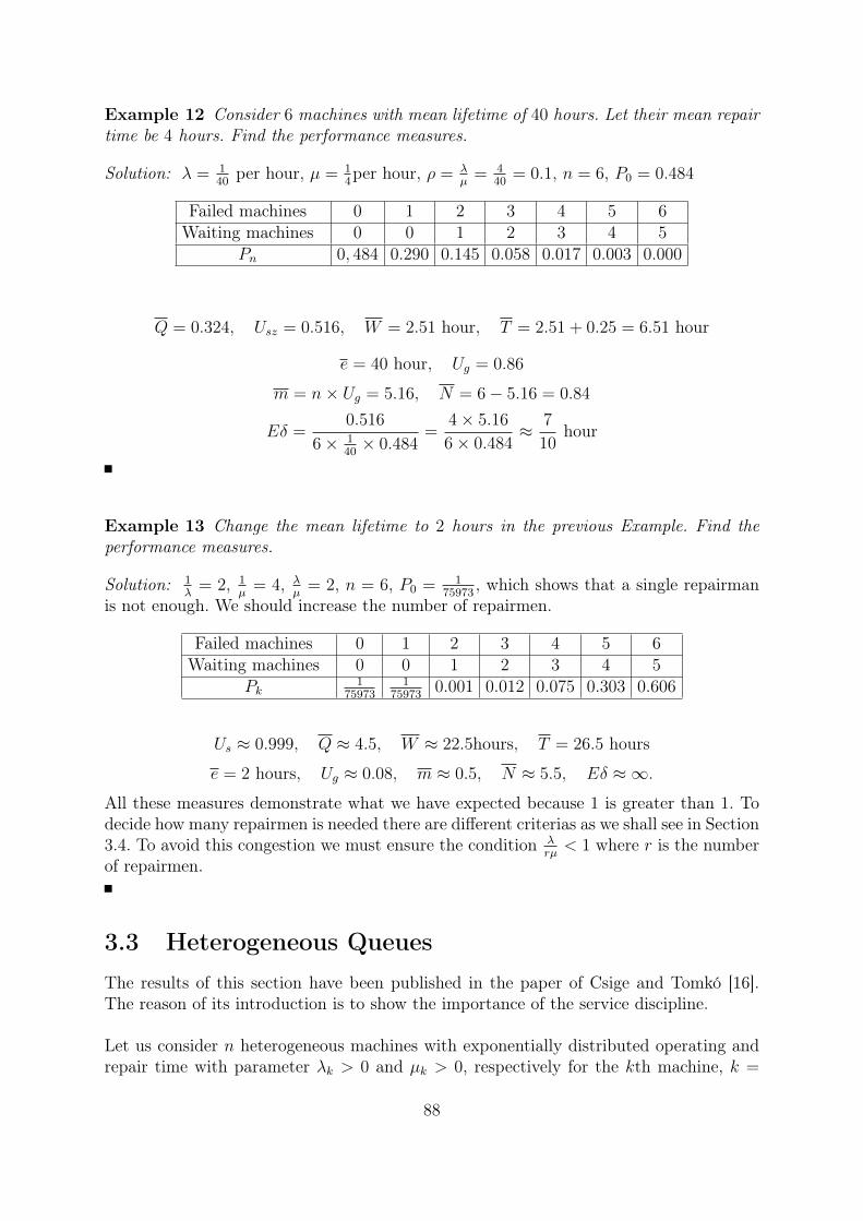
Example 12 Consider 6 machines with mean lifetime of 40 hours. Let their mean repairtime be 4 hours. Find the performance measures.
Solution: λ = 140
per hour, µ = 14per hour, ρ = λ
µ= 4
40= 0.1, n = 6, P0 = 0.484
Failed machines 0 1 2 3 4 5 6Waiting machines 0 0 1 2 3 4 5
Pn 0, 484 0.290 0.145 0.058 0.017 0.003 0.000
Q = 0.324, Usz = 0.516, W = 2.51 hour, T = 2.51 + 0.25 = 6.51 hour
e = 40 hour, Ug = 0.86
m = n× Ug = 5.16, N = 6− 5.16 = 0.84
Eδ =0.516
6× 140× 0.484
=4× 5.16
6× 0.484≈ 7
10hour
Example 13 Change the mean lifetime to 2 hours in the previous Example. Find theperformance measures.
Solution: 1λ
= 2, 1µ
= 4, λµ
= 2, n = 6, P0 = 175973
, which shows that a single repairmanis not enough. We should increase the number of repairmen.
Failed machines 0 1 2 3 4 5 6Waiting machines 0 0 1 2 3 4 5
Pk1
759731
759730.001 0.012 0.075 0.303 0.606
Us ≈ 0.999, Q ≈ 4.5, W ≈ 22.5hours, T = 26.5 hours
e = 2 hours, Ug ≈ 0.08, m ≈ 0.5, N ≈ 5.5, Eδ ≈ ∞.All these measures demonstrate what we have expected because 1 is greater than 1. Todecide how many repairmen is needed there are different criterias as we shall see in Section3.4. To avoid this congestion we must ensure the condition λ
rµ< 1 where r is the number
of repairmen.
3.3 Heterogeneous QueuesThe results of this section have been published in the paper of Csige and Tomkó [16].The reason of its introduction is to show the importance of the service discipline.
Let us consider n heterogeneous machines with exponentially distributed operating andrepair time with parameter λk > 0 and µk > 0, respectively for the kth machine, k =
88

1, · · · , n. The failures are repaired by a single repairman according to Processor Sharing,FIFO, and Preemptive Priory disciplines. All involved random variables are supposed tobe independent of each other.Let N(t), denote the number of failed machines at time t. Due to the heterogeneityof the machines this information is not enough to describe the behavior of the systembecause we have to know which machine is under service. Thus let us introduce an N(t)-dimensional vector with components
(x1 (t) , . . . , xv(t) (t)
)indicating the indexes of the
failed machines. Hence for N(t) > 0 using FIFO discipline machine with index x1(t) isunder service. Under Processor Sharing discipline when all machines are serviced by aproportional service rate, that is if N(t) = k then the proportion is 1/k the order ofindexes (x1 (t) , . . . , xn (t)) is not important, but a logical treatment we order them as(x1 (t) < x2 (t) < . . . < xv(t) (t)
). In the case of Preemptive Priority assuming that the
smaller index means higher priority we use the same ordering as before mentioning thatin this case the machine with the first index is under service since he has the highestpriority among the failed machines.Due to the exponential distributions the process
X(t) (t) =(v (t) ;x1 (t) , . . . , xv(t) (t)
), (t ≥ 0) ,
is a continuous-time Markov where the ordering of x1 (t) , . . . , xv(t) (t) depends ot theservice discipline.Since X(t)(t) is a finite state Markov chain thus if the parameters λk, µk, (1 ≤ k ≤ n)are all positive then it is ergodic and hence the steady-state distribution exists. Of coursethis heavily depends on the service discipline.
3.3.1 The ~M/ ~M/1/n/n/PS Queue
Let the distribution of the Markov chain be denoted by
P0(t), , P′
i1,...,ik(t).
It is not difficult to see that for this distribition we have
P′
0 (t) = −
[n∑i=1
λi
]P0 (t) +
n∑i=1
µiPi (t) ,
P′
i1,...,ik(t) =
k∑r=1
λirPi1,...,ir−1,ir+1,...,ik (t)−
−
[νi1...ik +
1
k
k∑r=1
µir
]Pi1,...,ik (t) +
∑r 6=i1...ik
µrk + 1
Pi′1i′2...i′k+1
(t)
where i′1, . . . , i′
k+1 is the ordering of the indexes i1, . . . , ik, r and
νi1...ik =∑
r 6=i1...ik
λr, k = 1, . . . , n− 1.
89

P′
1,...,n(t) =n∑r=1
λrP1,...,r−1,r+1,]...,n(t)−
[1
n
n∑r=1
µr
]P1,...,n(t).
The steady-state distribution which is denoted by
P0 = limt→∞
Po (t) ,
Pi1...ik = limt→∞
Pi1...ik (t)
(1 ≤ i1 < i2 < . . . < ik ≤ n, 1 ≤ k ≤ n).
is the solution of the following set of equations[n∑i=1
λi
]P0 =
n∑i=1
µiPi,
[νi1...ik +
1
k
k∑r=1
µir
]Pi1...ik =
k∑r=1
λirPi1...ir−1ir+1...ik+
+∑
r 6=i1...ik
µrk + 1
Pi′1i′2...i′k+1,
[1
n
n∑r=1
µr
]P1,...,n =
n∑r=1
λrP1...,r−1,r+1,...,n
with normalizing conditionP0 +
∑Pi1...ik = 1
where the summation is mean by all possible combinations of the indexes.
The surprising fact is it can be obtained as
Pi1...ik = Ck!k∏r=1
λirµir
,
where C can be calculated from the normalizing condition.
For the FIFO and Preemptive Priority disciplines the balance equations and the solutionis rather complicated and they are omitted. The interested reader is referred to the citedpaper. However for all cases the performance measures can be computed the same way.
Performance Measures
• Utilization of the server
Us =E(δ)
E(δ) +
[n∑i=1
λi
]−1 = 1− P0.
90

• Utilization of the machines
Let U (i) denote the utilization of machine i. Then
U (i) =1λi
1λi
+ T i= 1− P (i),
where T i denotes the mean response time for machine i, that is the mean time whileit is broken, and
P (i) =n∑k=1
∑i∈(i1,...,ik)
Pi1,...,ik ,
is the probability that the ith machine is failed. Thus
T i =P (i)
λi (1− P (i)),
and in FIFO case for the main waiting time we have
W i = T i −1
µi.
Furthermore it is easy to see that the mean number of failed machines can beobtained as
N =n∑i=1
P (i).
In additionn∑i=1
λi(1− P (i)
)T i =
n∑i=1
P (i)
which is the Little’s formula for heterogeneous customers. In particular, for ho-mogeneous case we
(n− N̄)λT̄ = N̄
which was proved earlier.
Various generalized versions of the machine interference problem with heterogeneous ma-chines can be found in Pósafalvi and Sztrik [62, 63].
Let us see some sample numerical results for the illustration of the influence of the servicedisciplines on the main performance measures
91
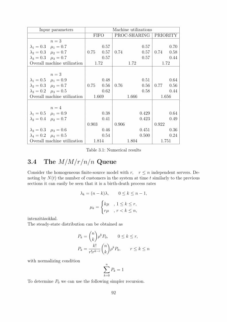
Inpur parameters Machine utilizationsFIFO PROC-SHARING PRIORITY
n = 3λ1 = 0.3 µ1 = 0.7 0.57 0.57 0.70λ2 = 0.3 µ2 = 0.7 0.75 0.57 0.74 0.57 0.74 0.58λ3 = 0.3 µ3 = 0.7 0.57 0.57 0.44Overall machine utilization 1.72 1.72 1.72
n = 3λ1 = 0.5 µ1 = 0.9 0.48 0.51 0.64λ2 = 0.3 µ2 = 0.7 0.75 0.56 0.76 0.56 0.77 0.56λ3 = 0.2 µ3 = 0.5 0.62 0.58 0.44Overall machine utilization 1.669 1.666 1.656
n = 4λ1 = 0.5 µ1 = 0.9 0.38 0.429 0.64λ2 = 0.4 µ2 = 0.7 0.41 0.423 0.49
0.903 0.906 0.922λ3 = 0.3 µ3 = 0.6 0.46 0.451 0.36λ4 = 0.2 µ4 = 0.5 0.54 0.500 0.24Overall machine utilization 1.814 1.804 1.751
Table 3.1: Numerical results
3.4 The M/M/r/n/n QueueConsider the homogeneous finite-source model with r, r ≤ n independent servers. De-noting by N(t) the number of customers in the system at time t similarly to the previoussections it can easily be seen that it is a birth-death process rates
λk = (n− k)λ, 0 ≤ k ≤ n− 1,
µk =
{kµ , 1 ≤ k ≤ r,rµ , r < k ≤ n,
intenzitásokkal.The steady-state distribution can be obtained as
Pk =
(n
k
)ρkP0, 0 ≤ k ≤ r,
Pk =k!
r!rk−r
(n
k
)ρkP0, r ≤ k ≤ n
with normalizing conditionn∑k=0
Pk = 1
To determine P0 we can use the following simpler recursion.
92
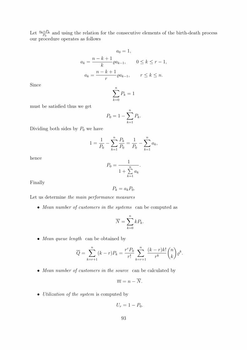
Let ak=PkP0
and using the relation for the consecutive elements of the birth-death processour procedure operates as follows
a0 = 1,
ak =n− k + 1
k%ak−1, 0 ≤ k ≤ r − 1,
ak =n− k + 1
r%ak−1, r ≤ k ≤ n.
Sincen∑k=0
Pk = 1
must be satisfied thus we get
P0 = 1−n∑k=1
Pk.
Dividing both sides by P0 we have
1 =1
P0
−n∑k=1
PkP0
=1
P0
−n∑k=1
ak,
henceP0 =
1
1 +n∑k=1
ak
.
FinallyPk = akP0.
Let us determine the main performance measures
• Mean number of customers in the systems can be computed as
N =n∑k=0
kPk.
• Mean queue length can be obtained by
Q =n∑
k=r+1
(k − r)Pk =rrP0
r!
n∑k=r+1
(k − r)k!
rk
(n
k
)%k.
• Mean number of customers in the source can be calculated by
m = n−N.
• Utilization of the system is computed by
Ur = 1− P0.
93
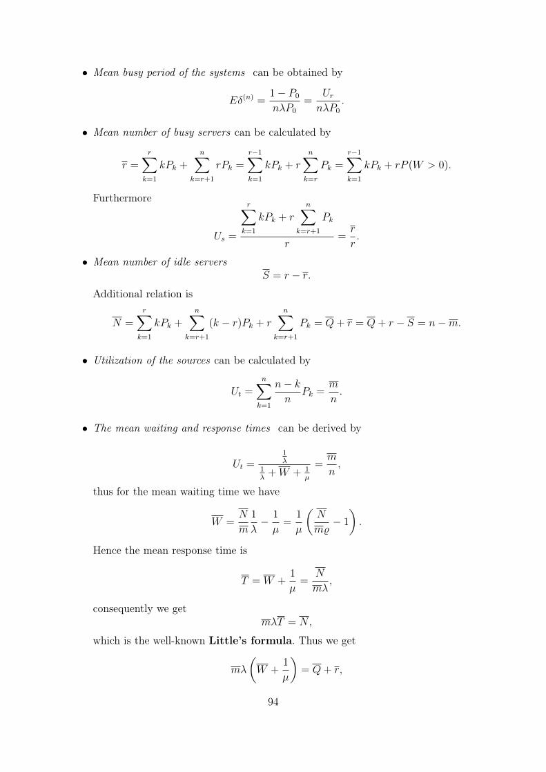
• Mean busy period of the systems can be obtained by
Eδ(n) =1− P0
nλP0
=UrnλP0
.
• Mean number of busy servers can be calculated by
r =r∑
k=1
kPk +n∑
k=r+1
rPk =r−1∑k=1
kPk + rn∑k=r
Pk =r−1∑k=1
kPk + rP (W > 0).
Furthermore
Us =
r∑k=1
kPk + rn∑
k=r+1
Pk
r=r
r.
• Mean number of idle serversS = r − r.
Additional relation is
N =r∑
k=1
kPk +n∑
k=r+1
(k − r)Pk + rn∑
k=r+1
Pk = Q+ r = Q+ r − S = n−m.
• Utilization of the sources can be calculated by
Ut =n∑k=1
n− kn
Pk =m
n.
• The mean waiting and response times can be derived by
Ut =1λ
1λ
+W + 1µ
=m
n,
thus for the mean waiting time we have
W =N
m
1
λ− 1
µ=
1
µ
(N
m%− 1
).
Hence the mean response time is
T = W +1
µ=
N
mλ,
consequently we getmλT = N,
which is the well-known Little’s formula. Thus we get
mλ
(W +
1
µ
)= Q+ r,
94
that ismλW +m% = Q+ r.
Show thatr = m%,
because from this followsmλW = Q
which is the Little’s formula for the waiting time.
SincePk+1 =
(n− k)λ
µk+1
Pk,
where
µj =
{jµ , j ≤ r,
rµ , j > r.
Furthermore, it is well-known that
r =r−1∑k=1
kPk + rn∑k=r
Pk.
We can proceed as
%m =n∑k=0
%(n− k)Pk =r−1∑k=0
%(n− k)Pk +n−1∑k=r
%(n− k)Pk =
=r−1∑k=0
λ(n− k)(k + 1)
(k + 1)µPk + r
n−1∑k=r
λ(n− k)
rµPk =
=r−1∑k=0
(k + 1)Pk+1 + rn−1∑k=r
Pk+1 =r∑j=1
jPj + rn∑
j=r+1
Pj =r−1∑j=1
jPj + rn∑j=r
Pj = r.
Finally we get%m = r,
or in another formλm = µr,
that ismean arrival rate = mean service rate,
which was expected because the system is in steady state. Consequently
W =Q
mλ=
Q
rλ%=
Q
µr.
95

• Mean idle period of a server can be computed as follows.If the idle servers start their busy period in the order as they finished the previousbusy period, then their activity can be written as follows. If a server becomes idleand finds other j − 1 servers idle, then his busy period start at the instant of thearrival of the j th customer.
Let e denote the mean idle period of the server and let ej denote the mean condi-tional idle period mention above. Clearly
ej =j
λ,
and e can be computed by the help of the theorem of total expectation, namely
e =r∑j=1
Pr−jP (e)
j
λ=
S
P (e)λ,
where
P (e) =r−1∑j=0
Pj = 1− P (W > 0),
is the probability that there is an idle server.
• Mean busy period of the servers can be calculated as follows.Since
Us =Eδ
e+ Eδ,
thus
Eδ =Us
1− Use =
rr
1− rr
e =rrr−rr
S
P (e)λ=r
S
S
P (e)λ=
r
P (e)λ=
m
µP (e).
That isEδ =
m
µP (e).
Distribution Function of the Waiting and Response Time
This subsection is devoted to the most complicated problem of this system, namely tothe determination of the distribution function of the waiting and response times. Firstthe density function is calculated and then we obtain the distribution function. You mayremember that the distribution has been given in the form
Pk =
(n
k
)ρkP0
(n
k
)k!ρk
r!rk−rP0.
96
Introducing z = 1ρ, this can be written as
Pk =
(n
k
)z−kP0
(n
k
)k!z−k
r!rk−rP0
thus
Pk =
(nk
)k!rr(rz)−k
r!P0
=n!rr(rz)n−k · e−rz
(n− k)!r!(rz)n · e−rzP0
=rr
r!
P (n− k, rz)
P (n, rz)P0, k ≥ r.
Since
Πk(n) = Pk(n− 1), thus
Πk(n) =rr
r!
P (n− 1− k, rz)
P (n− 1, rz)P0(n− 1), ha k = r, . . . , n− 1.
It is easy to see that the probability of waiting is
n−1∑k=r
Πk(n) =n−1∑k=r
Pk(n− 1) = PW
Inserting z this can be rewritten as
PW =n−1∑k=r
rr
r!
P (n− 1− k, rz)
P (n− 1, rz)P0(n− 1)
=rr
r!P0(n− 1)
n−1−r∑i=0
P (i, rz)
P (n− 1, rz)
=rr
r!
Q(n− 1− r, rz)P (n− 1, rz)
P0(n− 1).
We show that the distribution function of the waiting time can be calculated as
FW (x) = 1− rrQ(n− 1− r, r(z + µx))
r!P (n− 1, rz)P0(n− 1),
and thus
FW (0) = 1− rrQ(n− 1− r, rz)r!P (n− 1, rz)
P0(n− 1)
97
which is probability that an arriving customer finds idle server. For the density functionwe have
fW (0) = 1− PW ,
fW (x) = µrrrP (n− 1− r, r(z + µx))
r!P (n− 1, rz)P0(n− 1), x > 0.
If we calculate the integral∞∫
0+
fW (x)dx-t that is 0 is not considered then
∞∫0+
fW (x)dx =rrP0(n− 1)
r!P (n− 1, rz)·∞∫
0+
µr(r(z + µt))n−1−r
(n− 1− r)!e−r(z+µt)dt.
By the substitution y = r(z + µt) we have dtdy
= 1µfor the integral part we get
∞∫rz
yn−1−r
(n− 1− r)!e−ydy = Q(n− 1− r, rz)
that is∞∫
0+
fW (x)dx =rrQ(n− 1− r, rz)r!P (n− 1, rz)
P0(n− 1) = PW ,
as it was expected. Thus
∞∫0
fW (x)dx = fW (0) +
∞∫0+
fW (x)dx = 1.
Let us determine the density function for x > 0. That is
fW (x) =n−1∑k=r
rµ(rµx)k−r
(k − r)!e−rµxPk(n− 1)
=n−1∑k=r
rµ(rµx)k−r
(k − r)!e−rµx
rr
r!
P (n− 1− k, rz)
P (n− 1, rz)P0(n− 1)
=rµrrP0(n− 1)
r!P (n− 1, rz)
n−1∑k=r
(rµx)k−r
(k − r)!(rz)n−1−k
(n− 1− k)!e−r(z+µx)
=rµrrP0(n− 1)e−r(z+µx)
r!P (n− 1, rz)
n−1−r∑i=0
(rµx)i
i!
(rz)n−1−r−i
(n− 1− r − i)!
=rµrrP0(n− 1)
r!P (n− 1, rz)
(r(z + µx))n−1−r
(n− 1− r)!· e−r(z+µx)
=rµrrP0(n− 1)P (n− 1− r, r(z + µx))
r!P (n− 1, rz),
98
as we got earlier, but we have to remember that
fW (0) = 1− PW .
Therefore
P (W > x) =
∞∫x
fW (t)dt
=rrP0(n− 1)
r!P (n− 1, rz)
∞∫x
rµ(r(z + µt))n−1−r
(n− 1− r)!e−r(z+µt)dt
=rrP0(n− 1)
r!P (n− 1, rz)
∞∫r(z+µx)
yn−1−r
(n− 1− r)!e−ydy
=rrP0(n− 1)Q(n− 1− r, r(z + µx))
r!P (n− 1, rz).
Thus for the distribution function we have
FW (x) = 1− P (W > x)
which was obtained earlier.
To verify the correctness of the formula let r = 1. After substitution we get
P (W > x) =P0(n− 1)Q(n− 2, z + µx)
P (n− 1, z),
but
P0(n− 1) =P (n− 1, z)
Q(n− 1, z),
thus
P (W > x) =Q(n− z, z + µx)
Q(n− 1, z).
The derivation of the distribution function of the response time is analogous. Because thecalculation is rather lengthly it is omitted, but can be found in the Solution Manual forKobayashi [50].As it can be seen in Allen [2], Kobayashi [50], the following formulas are valid for r ≥ 2
FT (x) = 1− C1e−µx + C2Q(n− r − 1, r(z + µx)),
where
C1 = 1 + C2Q(n− r − 1, rz),
C2 =rrP0(n− 1)
r!(r − 1)(n− r − 1)!P (n− 1, rz).
99

Hence the density function can be obtained as
fT (x) = µC1e−µx − C2rµP (n− r − 1, r(z + µx)).
It should be noted that for the normalizing constant we have the following recursion
P−10 (n) = 1 +
n
rzP−1
0 (n− 1) +n
z
r−1∑i=0
(n−1i
)zi
(1
i+ 1− 1
r
), n > r,
with initial valueP−1
0 (r) =
(1 +
1
z
)r. r ≥ 1.
Laplace-transform of the Waiting and Response Times
First determine the Laplace-transform of the waiting time.It is easy to see that by using the theorem of total Laplace-transform we have
LW (s) = 1− PW +n−1∑k=r
(rµ
rµ+ s
)k−r+1
Pk(n− 1).
We calculate this formula step-by-step. Namely we can proceed as
n−1∑k=r
(rµ
rµ+ s
)k−r+1rrP0(n− 1)P (n− 1− k, rz)
r!P (n− 1, rz)
=rrP0(n− 1)e−rz
r!P (n− 1, rz)
n−1∑k=r
(rµ
rµ+ s
)k−r+1(rz)n−1−k
(n− 1− k)!.
Thenn−1∑k=r
(rµ
rµ+ s
)k−r+1(rz)n−1−k
(n− 1− k)!
=n−1−r∑i=0
(rµ
rµ+ s
)i+1(rz)n−1−r−i
(n− 1− r − i)!,
where i = k − r. Thus the last equation can be written as(rµ
rµ+ s
)n−r·n−1−r∑i=0
(rµ+zλ
)n−1−r−i
(n− 1− r − i)!=
(rµ
rµ+ s
)n−rerµ+zλ Q
(n− 1− r, rµ+ z
λ
).
Finally collecting all terms we get
LW (s) = 1− PW +
(rµ
rµ+ s
)n−rrrP0(n− 1)e−rz
r!P (n− 1, rz)erµ+sλ Q
(n− 1− r, rµ+ s
λ
)= 1− PW +
rresλP0(n− 1)Q
(n− 1− r, rµ+s
λ
)r!P (n− 1, rz)
(rµ
rµ+ s
)n−r.
100
To verify the correctness of the formula let r = 1.Thus after inserting we have
LW (s) = P0(n− 1) +
(µ
µ+ s
)n−1 esλP0(n− 1)Q
(n− 2, µ+s
λ
)P (n− 1, z)
=P (n− 1, z)
Q(n− 1, z)+
(µ
µ+ s
)n−1 esλQ(n− 2, µ+s
λ
)Q(n− 1, z)
=
(µµ+s
)n−1
Q(n− 1, z)
(z(µ+sµ
))n−1
(n− 1)!e−z + e
sλQ
(n− 2,
µ+ s
λ
)=
(µµ+s
)n−1
Q(n− 1, z)
[(µ+sλ
)n−1e−
µ+sλ e
sλ
(n− 1)!+ e
sλQ
(n− 2,
µ+ s
λ
)]
=
(µµ+s
)n−1
esλQ(n− 1, µ+s
λ
)Q (n− 1, z)
,
as we got earlier.
Keeping in mind the relation between the waiting time and the response time and theproperties of the Laplace-transform we have
LT (s) =
(µ
µ+ s
)LW (s),
which is in the case of r = 1 reduces to
LT (s) =
(µ
µ+ s
)n e sλQ (n− 1, µ+sλ
)Q(n− 1, z)
.
Java applets for direct calculations can be found athttp://irh.inf.unideb.hu/user/jsztrik/education/03/EN/MMcKK/MMcKK.html
Example 14 A factory possesses 20 machines having mean lifetime of 50 hours. Themean repair time is 5 hours and the repairs are carried out by 3 repairmen. Find theperformance measures of the system.
Solution:
ρ =λ
µ=
1µ
1λ
=5
50=
1
10= 0.1
By using the recursive approach we get
101
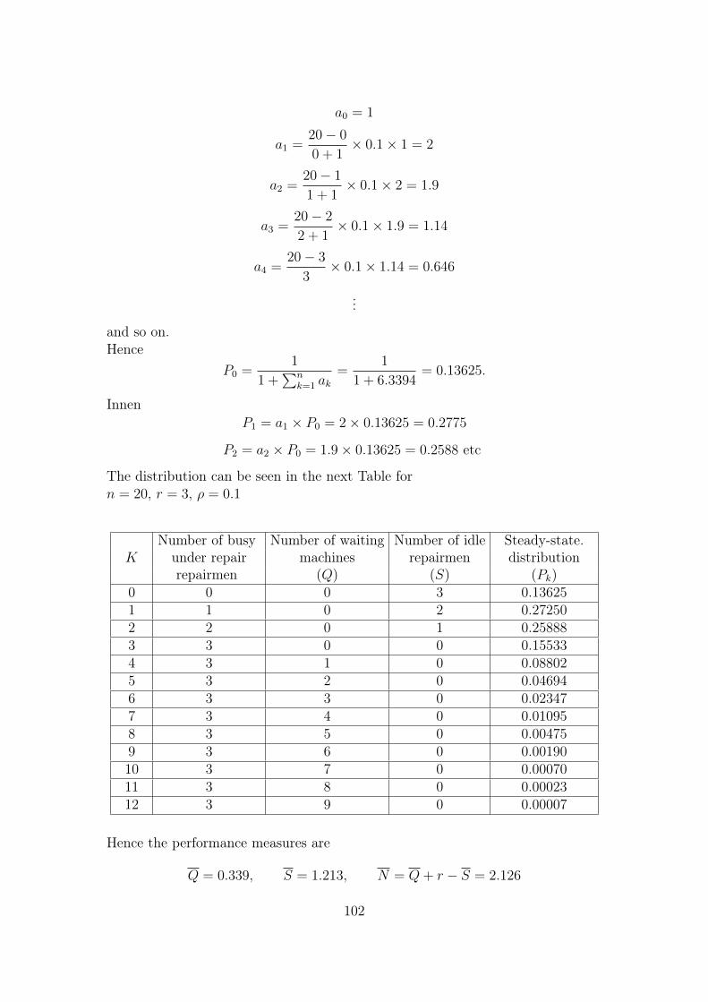
a0 = 1
a1 =20− 0
0 + 1× 0.1× 1 = 2
a2 =20− 1
1 + 1× 0.1× 2 = 1.9
a3 =20− 2
2 + 1× 0.1× 1.9 = 1.14
a4 =20− 3
3× 0.1× 1.14 = 0.646
...
and so on.Hence
P0 =1
1 +∑n
k=1 ak=
1
1 + 6.3394= 0.13625.
InnenP1 = a1 × P0 = 2× 0.13625 = 0.2775
P2 = a2 × P0 = 1.9× 0.13625 = 0.2588 etc
The distribution can be seen in the next Table forn = 20, r = 3, ρ = 0.1
Number of busy Number of waiting Number of idle Steady-state.K under repair machines repairmen distribution
repairmen (Q) (S) (Pk)0 0 0 3 0.136251 1 0 2 0.272502 2 0 1 0.258883 3 0 0 0.155334 3 1 0 0.088025 3 2 0 0.046946 3 3 0 0.023477 3 4 0 0.010958 3 5 0 0.004759 3 6 0 0.0019010 3 7 0 0.0007011 3 8 0 0.0002312 3 9 0 0.00007
Hence the performance measures are
Q = 0.339, S = 1.213, N = Q+ r − S = 2.126
102
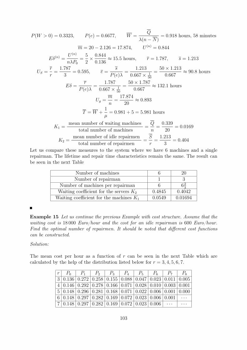
P (W > 0) = 0.3323, P (e) = 0.6677, W =Q
λ(n−N)= 0.918 hours, 58 minutes
m = 20− 2.126 = 17.874, U (n) = 0.844
Eδ(n) =U (n)
nλP0
=5
2× 0.844
0.136≈ 15.5 hours, r = 1.787, s = 1.213
US =r
r=
1.787
3= 0.595, e =
s
P (e)λ=
1.213
0.667× 150
=50× 1.213
0.667≈ 90.8 hours
Eδ =r
P (e)λ=
1.787
0.667× 150
=50× 1.787
0.667≈ 132.1 hours
Ug =m
n=
17.874
20≈ 0.893
T = W +1
µ= 0.981 + 5 = 5.981 hours
K1 =mean number of waiting machines
total number of machines=Q
n=
0.339
20= 0.0169
K2 =mean number of idle repairmen
total number of repairmen=S
r=
1.213
3= 0.404
Let us compare these measures to the system where we have 6 machines and a singlerepairman. The lifetime and repair time characteristics remain the same. The result canbe seen in the next Table
Number of machines 6 20Number of repairman 1 3
Number of machines per repairman 6 623
Waiting coefficient for the servers K2 0.4845 0.4042Waiting coefficient for the machines K1 0.0549 0.01694
Example 15 Let us continue the previous Example with cost structure. Assume that thewaiting cost is 18 000 Euro/hour and the cost for an idle repairman is 600 Euro/hour.Find the optimal number of repairmen. It should be noted that different cost functionscan be constructed.
Solution:
The mean cost per hour as a function of r can be seen in the next Table which arecalculated by the help of the distribution listed below for r = 3, 4, 5, 6, 7.
r P0 P1 P2 P3 P4 P5 P6 P7 P8
3 0.136 0.272 0.258 0.155 0.088 0.047 0.023 0.011 0.0054 0.146 0.292 0.278 0.166 0.071 0.028 0.010 0.003 0.0015 0.148 0.296 0.281 0.168 0.071 0.022 0.006 0.001 0.0006 0.148 0.297 0.282 0.169 0.072 0.023 0.006 0.001 · · ·7 0.148 0.297 0.282 0.169 0.072 0.023 0.006 · · · · · ·
103
The mean cost per hour is
r Q S E(Cost) Euro3 0.32 1.20 64804 0.06 2.18 23885 0.01 3.17 20826 0 4.17 25027 0 5.16 3096
Hence the optimal number is r = 5.This simple Example shows us that there are different criteria for the optimal operation.
3.5 The M/M/r/K/n QueueThis system is an combination of the finite-source systems considered in the previoussections. It is the most general system since for K = r we have the Engset system treatedin Section 3.1, for r = 1, K = n get the system analyzed in Section 3.2, for K = n weobtain the system of Section 3.4. For the value r < K < n we have delay-loss system,that is customers can arrive into the system until the number of customers in the systemis K − 1 but then the must return to the source because the system is full.As before it is easy to see that the number of customers in the systems is a birth-deathprocess with rates
λk = (n− k) , 0 ≤ k < K,
µk =
{kµ , 1 ≤ k ≤ r,rµ , r < k ≤ K
where 1 ≤ r ≤ n, r ≤ K ≤ n. It is qiute complicated system and have not beeninvestigated, yet. The main problem is that there are no closed form formulas as before,but using computers all the performance measures can be obtained. The normalizingconstant P0(n, r,K) should satisfies the normalizing condition
K∑i=0
Pk(n, r,K) = 1.
As before it can easily be seen that
Pk(n, r,K) =
(n
k
)ρkP0(n, r,K) , 0 ≤ k < r,
(n
k
)k!ρk
r!rk−rP0(n, r,K) , r ≤ k ≤ K
104
The main performance measures can be computed as
N =K∑k=0
kPk, Q =K∑k=r
(k − r)Pk, r =r−1∑k=1
kPk + rK∑k=r
Pk, m = n−N,
US =r
r, Ut =
n−Nn
, λ = µ = µr,
T =N
λ, W =
Q
λ, W = T − 1
µ,
n−Nn
=E(τ)
E(τ) + T, E(τ) =
(n−N)T
N, NR = E(τ)λ.
By using the Bayes’s rule it is easy to see that for the probability of blocking we have
PB(n, r,K) =(n−K)PK(n, r,K)K∑i=0
(n− i)Pi(n, r,K)
= PK(n− 1, r,K).
In particular, if K = n, then
λ = λ(n−N) = µr,
thus
T =N
λ(n−N), E(τ) =
1
λ, PB = 0,
as it was expected.Furthermore, by elementary calculations it can be seen that the normalizing constantP0(n, r,K) can be expressed recursively with respect to K under fixed r, n. Namely wehave
(P0(n, r,K))−1 = (P0(n, r,K − 1))−1 +
(nK
)K!ρK
r!rK−r,
with initial value
(P0(n, r, r))−1 =r∑i=0
(n
i
)ρi.
By using the Bayes’s rule it is easy to see that the probability that an arriving customerfinds k customers in the system is
Π∗k(n, r,K) = Pk(n− 1, r,K), k = 0, · · · , K
105
but the probability that a customer arriving into the systems finds k customers there is
Πk(n, r,K) =(n− k)Pk(n, r,K)
K−1∑i=0
(n− i)Pi(n, r,K)
, k = 0, . . . , K − 1.
Hence the probability of waiting and the density function of the waiting time can beexpressed as
PW (n, r,K) =K−1∑k=r
Πk(n, r,K)
fW (0) = 1− PW (n, r,K)
fW (x) =K−1∑k=r
(rµ)(rµx)k−r+1
(k − r + 1)!e−rµx · Πk(n, r,K)
By using the Bayes’s rule it can easily be verified that
Πk(n, r,K) =Pk(n− 1, r,K)
1− PK(n− 1, r,K),
and analogously to the earlier arguments for the density function we obtain
fW (x) =µrrrP (K − 1− r, rz)
r!P (K − 1, rz)
P0(n− 1)
1− PK(n− 1, r,K).
In paricular, if K = n, that is all customer may enter into the system, thenPK(n− 1, r,K) = 0 and thus we got the formulas derived before.
By reasonable modifications for the distribution function we have
FW (x) = 1− rrQ(K − 1− r, r(z + µx))
r!P (K − 1, rz)
P0(n− 1, r,K)
1− PK(n− 1, r,K).
The corresponding Laplace-transform can be computed as
LW (s) = 1− PW (n, r,K) +
(rµ
rµ+ s
)Krre
sλ
r!
Q(K − 1− r, rµ+s
λ
)P0(n− 1, r,K)
P (K − 1, rz)(1− PK(n− 1, r,K)).
3.6 The M/G/1/n/n/PS Queue
This system is a generalization of system M/M/1/n/n/FIFO treated in Section 3.2.The essential differences are the distribution of the service time and the service disciple.Since the service times are not exponentially distributed the number of customers as astochastic process is not a Markov chain. In this Section we introduce the model whichhas been published in Yashkov [101].
106
The requests arrive from a finite-source where they spend an exponentially distributedtime with parameter λ. The required service time S is generally distributed random vari-able with ES < ∞. Let us denote by G(x) and g(x) its distribution function, densityfunction, respectively, assuming that (G (0+) = 0). The service discipline is ProcessorSharing, that is all customers in the service facility are being served but the rate is pro-portional to the number of customers in service.
The method of supplementary variables is used for the description of the behavior of thesystem.Let us introduce the following random variables.Let ν(t) denote the number of customers in the system at time t, and for ν(t) > 0 letξ1(t), . . . , ξν(t)(t) denote the elapsed service time of the requests.
The stochastic processX(t) =
(ν(t); ξ1(t), . . . , ξν(t)(t)
)is a continuous-time Markov process with discrete and continuous components which arecalled piecewise linear Markov process.
It should be noted the many practical problems can be modeled by the help of theseprocesses and the interested reader is referred to the book of Gnedenko–Kovalenko [31].
Let
Pk (t, x1, . . . , xk) dx1 . . . dxk = P (ν(t) = k;xi ≤ ξi < xi + dxi, i = 1, . . . , k) ,
that is Pk(t, x1, . . . , xk), k = 1, . . . , n denotes the density function that at time t thereare k customers in the system and their elapsed service times are x1, . . . , xk.Let δ be a small positive real number. Then for the density functions Pk(t, x1, . . . , xk) wehave the following set of equations
Pk (t;x1, . . . , xk) =
= Pk
(t− δ;x1 −
δ
k, . . . , xk −
δ
k
) k∏i=1
1−G (xi)
1−G(xi − δ
k
) [1− λ (n− k) δ] +
+ (k + 1)
∞∫0
Pk+1
(t− δ;x1 −
δ
k, . . . , xk+1 −
δ
k + 1
)×
×k∏i=1
1−G (xi)
1−G(xi − δ
k+1
) · G (xk+1)−G[xk+1 − δ
k+1
]1−G
[xk+1 − δ
k+1
] dxk+1.
Dividing both sides byk∏i=1
[1−G (xi)] and taking the limits as δ → 0, t → ∞ we have
the stationary equations, namely[1
k
k∑i=1
∂
∂xi+ λ (n− k)
]qk
(x1, . . . , xk) =
107
∞∫0
qk+1
(x1, . . . , xk+1) g (xk+1) dxk+1, k = 1, . . . , n− 1,
where
qk (x1, . . . , xk) = limt→∞
Pk (t;x1, . . . , xk) /k∏i=1
[1−G (xi)]
are called normalized density functions.
Similarly, for P0 and qn(x1, . . . , xn) we obtain
λnP0 =
∞∫0
q1 (x1) g (x1) dx1,
1
n
n∑i=1
∂
∂xiqn (x1, . . . , xn) = 0.
Beside these equation we need the boundary conditions which are
q1 (0) = λnP0,
qk (0, x1, . . . , xk−1) = λ (n− k + 1) qk−1 (x1, . . . , xk−1) ,
k = 1, . . . , n.
The solution to these set of integro-differential equations is surprisingly simple, namely
qk (x1, . . . , xk) = P0λkn!/ [(n− k)!] ,
which can be proved by direct substitution.Consequently
Pk (x1, . . . , xk) = P0λk n!
(n− k)!
k∏i=1
[1−G (xi)] ,
i = 1, . . . , n.
Let us denote by Pk the steady-state probability of the number of customers in the system.Clearly we have
Pk =
∞∫0
. . .
∞∫0
Pk (x1, . . . , xk) dx1 . . . dxk = P0n!
(n− k)!(λES)k.
Probability P0 can be obtained by using the normalizing conditionn∑i=0
Pi = 1.
Recall that it is the same as the distribution in the M/M/1/n/n system if % = λES.
108

It is not difficult to see that for this M/G/1/n/n/PS system the performance measurescan be calculated as
(i) N =n∑k=1
kPk
(ii) U (i) =1λ
1λ
+ T=n−Nn
,
thus
T =1
λ
N
n−N,
hence
λ(n−N)T = N
which is the Little’s formula.Clearly, due to the Processor Sharing discipline the response time is longer then the re-quired service time, and there is no waiting time since each customer are being served.The difference is T − E(S).
It can be proved, see Cohen [14], that for an ~G/~G/1/n/n/PS system the steady-stateprobability that customers with indexes i1, . . . , ik are in the system can be written as
P (i1, . . . , ik) = C · k!k∏j=1
ρij, ρi =E(Si)
E(τi), i = 1, . . . , n.
For homogeneous case we get
Pk = C · k!
(n
k
)ρk.
3.7 The ~G/M/r/n/n/FIFO QueueThis section is devoted to a generalized version the finite-source model with multipleservers where the customers are supposed to have heterogeneous generally distributedsource times and homogeneous exponentially distributed service times. They are servedaccording to the order of their arrivals. The detailed description of this model can befound in Sztrik [77].
Customers arrive from a finite source of size n and are served by one of r (r ≤ n)servers at a service facility according to a first-come first-served (FFIFO) discipline. Ifthere is no idle server, then a waiting line is formed and the units are delayed. The servicetimes of the units are supposed to be identically and exponentially distributed randomvariables with parameter µ. After completing service, customer with index i returns tothe source and stays there for a random time τi having general distribution function Fi(x)with density fi(x). All random variables are assumed to be independent of each other.
109

Determination of the steady-state distribution
As in the previous section the modeling is more difficult since the involved random timesare not all exponentially distributed and thus we have to use the method of supplementaryvariables.
Let the random variable ν(t) denote the number of customers staying in the source attime t and let
(α1 (t) , . . . , αν(t)
)indicate their indexes ordered lexicographically, that is
in increasing order of their indexes.
Let us denote by(β1 (t) , . . . , βn−ν(t)
)the indexes of the requests waiting or served at the
service facility in the order of their arrival. It is not difficult to see that the process
Y (t) =(ν (t) ;α1 (t) , . . . , αν(t); β1 (t) , . . . , βn−ν(t)
), (t ≥ 0)
is not Markovian unless the distribution functions Fi (x) , i = 1, . . . , n are exponential.
To use the supplementary variable technique let us introduce the supplementary variableξαi (t) to denote the elapsed source time of request with index αi, i = 1, · · · , n. Define
X (t) =(ν (t) ;α1 (t) , . . . , αν(t); ξα1 (t) , . . . , ξαν(t); β1 (t) , . . . .βn−ν(t)
)This is a multicomponent piecewise linear Markov process.
Let V nk and Cn
k denote the set of all variations and combinations of order k of the in-tegers 1, 2, . . . , n, respectively, ordered lexicographically. Then the state space of process(X (t) , t ≥ 0) consists of the set of points
(i1, . . . , ik;x1, . . . , xk; j1, . . . , jn−k)
where
(i1, . . . , ik) ∈ Cnk , (j1, . . . , jn−k) ∈ V n
k , xi ∈ R+, i = 0, 1, . . . , k, k = 0, 1, . . . , n.
Process X(t) is in state (i1, . . . , ik;x1, . . . , xk; j1, . . . , jn−k) if k customers with indexes(i1, . . . , ik) have been staying in the source for times (x1, . . . , xk), respectively while therest need service and their indexes in the order of arrival are (j1, . . . , jn−k).
To derive the Kolmogorov-equations we should consider the transitions that can occur inan arbitrary time interval (t, t + h) . For 0 ≤ n − k < r the transition probabilities arethen the following
P [X (t+ h) = (i1, . . . , ik;x1 + h, . . . , xk + h; j1, . . . , jn−k) |
X (t) = (i1, . . . , ik;x1, . . . , xk; j1, . . . , jn−k)]
= (1− (n− k)µh)k∏l=1
1− Fil (xl + h)
1− Fil (xl)+ o (h) ,
P [X (t+ h) = (i1, . . . , ik;x1 + h, . . . , xk + h; j1, . . . , jn−k) |
110
X (t) = (i′
1, . . . , j′
n−k, . . . , i′
k;x′
1, . . . , y′, . . . , x
′
k; j1, . . . , jn−k−1)]
=fjn−k (y)h
1− Fjn−k (y)
k∏l=1
1− Fil (xl + h)
1− Fil (xl)+ o (h) ,
where (i′1, . . . , j
′
n−k, . . . , i′
k) denotes the lexicographical order of indexes (i1, . . . , ik, jn−k)while (x1
′, . . . , y′, . . . , x
′
k) indicates the corresponding times.For r ≤ n− k ≤ n the transition probabilities can be obtained as
P [X (t+ h) = (i1, . . . , ik;x1 + h, . . . , xk + h; j1, . . . , jn−k) |
X (t) = (i1, . . . , ik;x1, . . . , xk; j1, . . . , jn−k)]
= (1− rµh)k∏l=1
1− Fil (xl + h)
1− Fil (xl)+ o (h) ,
P[X (t+ h) = (i1, . . . , ik;x1 + h, . . . , xk + h; j1, . . . , jn−k) |
X (t) =(i′
1, . . . , j′
n−k, . . . , ik;x1, . . . , y′, . . . , x
′
k; j1, . . . , jn−k−1
)]=
=fjn−k (y)h
1− Fjn−k (y)
k∏l=1
1− Fil (xl + h)
1− Fil (xl)+ o (h) .
For the distribution of X(t) introduce the following functions
Q0;j1,...,jn (t) = P (ν (t) = 0; β1 (t) = j1, . . . , βn (t) = jn) ,
Qi1,...,ik;j1,...,jn−k (x1, . . . , xk; t) =
P (ν (t) = k;α1 (t) = i1, . . . , αk (t) = ik; ξi1 ≤ x1, . . . , ξik ≤ xk;
β1 (t) = j1, . . . , βn−k (t) = jn−k) .
Let λi is defined by 1/λi = E(τi). Then we have
Theorem 2 If 1/λi < ∞, i = 1, . . . , n, then the process (X (t) , t ≥ 0) possesses aunique limiting ( stationary, steady-state) distribution independent of the initial condi-tions, namely
Q0;j1,...,jn = limt→∞
Q0;j1,...,jn (t) ,
Qi1,...,ik;j1,...,jn−k (x1, . . . , xk) = limt→∞
Qi1,...,ik;j1,...,jn−k (x1, . . . , xk; t) .
Notice that X(t) belongs to the class of piecewise-linear Markov processes, subject todiscontinuous changes treated by Gnedenko and Kovalenko [31]. Our statement followsfrom a theorem on page 211 of this monograph.
Since by assumption Fi(x) has density function, for fixed k Theorem 2 provides theexistence and uniqueness of the following limits
qi1,...,ik;j1,...,jn−k (x1, . . . , xk) dx1 . . . dxk =
111
= P (ν (t) = k;α1 (t) = i1, . . . , αk (t) = il;xl ≤ ξil < xl + dxl, l = 1, . . . , k;
β1 (t) = j1, . . . , βn−k (t) = jn−k) , k = 1, . . . , n
where qi1,...,ik;j1,...,jn−k (x1, . . . , xk) denotes the density function of state(i1, . . . , ik;x1, . . . , xk; j1, . . . , jn−k) when t→∞.
Let us introduce the so-called normed density function defined by
q̃i1,...,ik;j1,...,jn−k (x1, . . . , xk) =qi1,...,ik;j1,...,jn−k (x1, . . . , xk)
(1− Fi1 (x1)) . . . (1− Fik (xk)).
Then we have
Theorem 3 The normed density functions satisfy the following system of integro-differentialequations (3.1), (3.3) with boundary conditions (3.2), (3.4)
(3.1)[∂
∂x1
+ . . .+∂
∂xk
]∗q̃i1,...,ik;j1,...,jn−k (x1, . . . , xk)
= − (n− k)µq̃i1,...,ik;j1,...,jn−k (x1, . . . , xk) +
+
∞∫0
q̃i′1,...,j′n−k,...,i
′k;j1,...,jn−k−1
(x′
1, . . . , y′, . . . , x
′
k
)fjn (y) dy,
(3.2) q̃i1,...,ik;j1,...,jn−k (x1, . . . , xl−1, 0, xl+1, . . . , xk) =
= µ∑
Vilj1,...,jn−k
q̃i1,...,il−1;il+1,...,ik;j1,...,jn−k (x1, . . . , xl−1, xl+1, . . . , xk)
for l = 1, . . . , k, 0 ≤ n− k < r
(3.3)[∂
∂x1
+ . . .+∂
∂xk
]∗q̃i1,...,ik;j1,...,jn−k (x1, . . . , xk) =
= −rµq̃i1,...,ik;j1,...,jn−k (x1, . . . , xk) +
+
∞∫0
q̃i′1,...,j′n−k,...,i
′k;j1,...,jn−k−1
(x′
1, . . . , y′, . . . , x
′
k)fjn(y)dy
(3.4) q̃i1,...,ik;j1,...,jn−k (x1, . . . , xl−1, 0, xl+1, . . . , xk) =
= µ∑
Vilj1,...,jr−1
q̃i1,...,il−1;il+1,...,ik;j1,...,jn−k (x1, . . . , xl−1, xl+1, . . . , xk) ,
for l = 1, . . . , k, r ≤ n− k < n− 1
112

furthermore
rµQ0;j1,...,jn =
∞∫0
q̃jn;j1,...,jn−1(y)fjn (y) dy.
The symbol [ ]∗ will be explained later while
V ilj1,...,js
= [(il, j1, . . . , js) , (j1, il, j2, . . . , js) , . . . , (j1, . . . , js, il)] ∈ V ns+1.
Proof: Since the process (X (t) , t ≥ 0) is Markovian its densities must satisfy the Kolmogorov-equations. A derivation is based on the examination of the sample paths of the processduring an infinitesimal interval of width h. The following relations hold
qi1,...,ik;j1,...,jn−k (x1 + h, . . . , xk + h) =
= qi1,...,ik;j1,...,jn−k (x1, . . . , xk) (1− (n− k)µh)k∏l=1
1− Fil (xl + h)
1− Fil (xl)+
+k∏l=1
1− Fil (xl + h)
1− Fil (xl)+
∞∫0
q̃i′1,...,j′n−k,...,i
′k;j1,...,jn−k−1
(x′
1, . . . , y′. . . , x
′
k
)×
×f′jn−k
(y)h
1− Fjn−k (xl)dy + o (h) ,
qi1,...,ik;j1,...,jn−k (x1 + h, . . . , xl−1 + h, 0, xl+1 + h, . . . , xk + h)h =
= o (h) +k∏s=1s 6=l
1− Fis (xs + h)
1− Fis (xs)×
×µh∑
Vilj1,...,jn−k
q̃i1,...,il−1;il+1,...,ik;j1,...,jn−k (x1, . . . , xl−1, xl+1, . . . , xk)
for 0 ≤ n− k < r, l = 1, . . . , k.Similarly
qi1,...,ik;j1,...,jn−k (x1 + h, . . . , xk + h) =
= qi1,...,ik;j1,...,jn−k (x1, . . . , xk) (1− rµh)k∏l=1
1− Fil (xl + h)
1− Fil (xl)+
+k∏l=1
1− Fil (xl + h)
1− Fil (xl)
∞∫0
q̃i′1,...,j′n−k,...,ie
′k;j1,...,jn−k−1
(x′
1, . . . , y′, . . . , x
′
k
)×
×f′jn−k
(y)h
1− Fjn−k (xl)dy + o (h) ,
qi1,...,ik;j1,...,jn−k (x1 + h, . . . , xl−1 + h, 0, xl+1 + h, . . . , xk + h)h =
113

= o (h) +k∏s=1s 6=l
1− Fis (xs + h)
1− Fis (xs)×
×µh∑
Vilj1,...,jn−k
q̃i1,...,il−1;il+1,...,ik;j1,...,jn−k (x1, . . . , xl−1, xl+1, . . . , xk)
for 0 ≤ n− k < r, l = 1, . . . , k.Finally
Q0;j1,...,jn = Q0;j1,...,jn (1− rµh) +
+
∞∫0
q̃jn;j1,...,jn−1 (y)fjn (y)h
1− Fjn (y)dy + o (h) .
Thus the statement of this theorem can easily be obtained. Dividing the left-hand side
of equations byk∏l=1
(1− Fil (xl + h)) and taking into account the definition of the normed
densities taking the limit as h→ 0 we get the desired result.
In the left-hand side of (3.1)(3.3) used for the notation of the limit in the right-hand side,the usual notation for partial differential quotients has been applied. Strictly consideringthis is not allowed, since the existence of the individual partial differential quotient is notassured. This is why the operator is notated by [ ]∗. Actually this is a (1, 1, . . . , 1) ∈ Rk
directional derivative, see Cohen [14].
To determine the steady-state probabilities[Q0;j1,...,jn , Qi1,...,ik;j1,...,jn−k
],
(i1, . . . , ik) ∈ Cnk , (j1, . . . , jn−k) ∈ V N
n−k, k = 1, . . . , n.
we have to solve equations (3.1)(3.3) subject to the boundary conditions (3.2)(3.4).If we set
Q0;j1,...,jn = c0,
q̃i1,...,ik;j1,...,jn−k (x1, . . . , xk) = ck, k = 1, . . . , n,
then by direct substitution it can easily be verified that they satisfy these equations withboundary conditions. Moreover these ck can be obtained by the help of cn, namely
ck =(r!rn−r−kµn−k
)−1cn, 0 ≤ k ≤ n− r,
ck =((n− k)!µn−k
)−1cn, n− r ≤ k ≤ n.
Since these equations completely describe the system, this is the required solution.
Let Qi1,...,ik;j1,...,jn−k denote the steady-state probability that customers with indexes(i1, . . . , ik) are in the source and the order of arrivals of the rest to the service facilityis (j1, . . . , jn−k). Furthermore, denote by Qi1,...,ik the stationary probability that requestswith indexes (i1, . . . , ik) i are staying in the source.
114

It can easily be seen
Qi1,...,ik;j1,...,jn−k = (λi1 , . . . , λik)−1ck, k = 1, . . . , n.
By using the relation we obtained for ck we have
Qi1,...,ik = (n− k)!(r!rn−r−kµn−kλi1 , . . . , λik
)−1cn,
(i1, . . . , ik) ∈ Cnk , k = 0, 1, . . . , n− r.
SimilarlyQi1,...,ik =
(µn−kλi1 , . . . , λik
)−1cn,
(i1, . . . , ik) ∈ Cnk , k = n− r, . . . , n.
Let us denote by Q̂k and P̂l the steady-state probability of the number of customers inthe source, in the service facility, respectively. Hence it is easy to see that
Qi1,...,in = Q1,...,n = Q̂n,
Q̂k = P̂n−k, k = 0, . . . , n.
Furthermorecn = Q̂n (λ1, . . . , λn) ,
Q̂k =∑
(i1,...,ik)∈Cnk
Qi1,...,ik ,
where Q̂n can be obtained by the help of the normalizing conditionn∑k=0
Q̂k = 1.
In the homogeneous case these formulas reduce to
Q̂k =n!
r!k!rn−k−r
(λ
µ
)n−kQ̂n, for 0 ≤ k ≤ n− r,
Q̂k =
(n
k
)(λ
µ
)n−kQ̂n, for n− r ≤ k ≤ n,
which is the result of the paper Bunday and Scraton [12], and for r = 1 is the formulasobtained by Schatte [72]. Thus the distribution of the number of customers in the servicefacility is
P̂k =
(n
k
)(λ
µ
)kP̂0, for 0 ≤ k ≤ r,
P̂k =n!
r!(n− k)!rk−r
(λ
µ
)kP̂0, for r ≤ k ≤ n.
This is exactly the same result that we got for the < M/M/r/n/n > model.
It should be underlined that the distribution of the number of customers in the systemdoes not depend on the form of Fi(x) but the mean 1/λi, that is it is robust.
115

Performance Measures
• Utilization of the sourcesLet Q(i) denote the steady-state distribution that source i is busy with generatinga new customer, that is
Q(i) =n∑k=1
∑i∈(i1,...,ik)∈Cnk
Qi1,...,ik .
Hence the utilization of source i can be obtained as
U (i) = Q(i).
• Utilization of the serversAs we have calculated earlier the utilization of a server can be derived as
UCPU =1
r
(r∑
k=1
kP̂k + r
n∑k=r+1
P̂k
)=r̄
r,
where r̄ denotes the mean number of busy servers. Thus the overall utilization ofthe servers is r̄.
• Mean waiting and response timesBy the results of Tomkó [92] we have
Q(i) = (1/λi)(1/λi + W̄i + 1/µ
)−1.
Thus for the mean waiting time of the customer with index i we obtain
W̄i =1
λi· 1−Q(i)
Q(i)− 1
µ, i = 1, . . . , n.
Consequently the mean response time T̄i of the ith request can be calculated as
T̄i = W̄i + 1/µ =(1−Q(i)
) (λiQ
(i))−1
, i = 1, . . . , n.
Sincen∑i=1
(1−Q(i)
)= N̄ ,
where N̄ denotes the mean number customers at the service facility. This can berewritten as
n∑i=1
λiT̄iQ(i) = N̄ ,
which the Little’s formula for the ~G/M/r/n/n/FIFO > queueing system.
It should be noted that using the terminology of the machine interference problem U (i),W̄i, T̄i denote the utilization, mean waiting time and the mean time spent in a brokenstate of the ith machine.
This model can be generalized such a way that the service intensities depend on thenumber of customers in the source, see Sztrik [79, 80].
116

Part II
Exercises
117


Chapter 4
Infinite-Source Systems
Exercise 1 Solve the following system of equations by the help of difference equations
λP0 = µP1
(λ+ µ)Pn = λPn−1 + µPn+1, n ≥ 1.
Solution:It is easy to see that it can be rewritten as
λPn−1 − (λ+ µ)Pn + µPn+1 = 0, n = 1, 2, . . .
which is a 2-nd order difference equation with constant coefficient. Its general solutioncan be obtained in the form
Pn = c1xn1 + c2x
n2 , n = 1, 2, . . .
where x1, x2 are the solutions to
µx2 − (λ+ µ)x+ λ = 0.
It can easily be verified that x1 = 1, x2 = % and thus
Pn = c1 + c2%n, n = 1, 2, . . . .
However P1 = %P0, and because∑∞
n=0 Pn = 1, thus c1 = 0 and c2 = P0 = 1− %.
Exercise 2 Find the generating function of the number of customers in the system foran M/M/1 queueing system by using the steady-state balance equations. Then derive thecorresponding distribution.
Solution:Staring with the set of equations
λP0 = µP1
(λ+ µ)Pn = λPn−1 + µPn+1, n ≥ 1
119
by multiplying both sides by si and then adding the terms we obtain
λGN(s) + µGN(s)− µP0 = λsGN(s) +µ
sGN(s)− µ
sP0.
Thus we can calculate as
GN(s)
(λ(1− s) + µ
(1− 1
s
))= µ
(1− 1
s
)P0,
GN(s)
(µ
(1− 1
s
)− λs
(1− 1
s
))= µ
(1− 1
s
)P0,
GN(s) =µ
µ− λsP0.
Since GN(1) = 1, therefore
P0 =µ− λµ
= 1− %.
That isGN(s) =
1− %1− s%
,
which is exactly the generating function of a modified geometric distribution with pa-rameter (1− %). It can be proved as follows, if
P (N = k) = (1− %)%k, k = 0, . . .
then its generating function is
GN(s) =∞∑k=0
sk(1− %)%k =1− %1− s%
.
Exercise 3 Find the generating function of the number of customers waiting in a queuefor an M/M/1 queueing system.
Solution:Clearly
GQ(s) = (P0 + P1)s0 +∞∑k=2
sk−1Pk = P0 +∞∑k=1
sk−1Pk = 1− %+∞∑k=1
sk−1%k(1− %)
= 1− %+ %∞∑i=0
si(1− %)%i = 1− %+ %GN(s) = 1− %(1−GN(s)).
For verification let us calculate the mean queue length, thus
G′Q(1) = %G′N(1) =%2
1− %.
120
Exercise 4 Find the Laplace-transform of T and W for an M/M/1 queueing system.
Solution:It is easy to see that
LT (s) =∞∑k=0
(µ
µ+ s
)k+1
%k(1− %) = (1− %)µ
µ+ s
∞∑k=0
(µ%
µ+ s
)k= (1− %)
µ
µ+ s
1
1− µ%µ+s
= (1− %)µ
µ+ s
µ+ s
µ(1− %) + s=
µ(1− %)
µ(1− %) + s,
which was expected, since T follows an exponential distribution with parameter µ(1−%).To get the Laplace-transform of W we have
LW (s) =∞∑k=0
(µ
µ+ s
)k%k(1− %) = 1− %+
∞∑k=1
(µ
µ+ s
)k%k(1− %)
= 1− %+%µ(1− %)
µ(1− %) + s,
which should beLT (s)
µµ+s
sinceLT (s) = LW (s)
µ
µ+ s.
To show this it can be calculated that
LW (s) = LT (s)µ+ s
µ=
µ(1− %)
µ(1− %) + s
µ+ s
µ= 1− %+ %
µ(1− %)
µ(1− %) + s.
Let us verify the result by deriving the mean values T and W .
L′T (0) = − 1
µ(1− %),
L′W (0) = %L′T (0) = − %
µ(1− %),
thusT =
1
µ(1− %),W =
%
µ(1− %),
which was obtained earlier.
Exercise 5 Show that for an M/M/1/K queueing system
limK→∞
N(K) =ρ
1− ρ, ρ < 1
.
121
Solution:It is well-known if ρ < 1 then
limK→∞
ρK = 0.
Since N =ρ(1−(K+1)ρK+KρK+1)
(1−ρ)(1−ρK+1), it is enough to show that
limK→∞
KρK = 0.
This can be proved by the L’Hospital’s rule, namely
limK→∞
K
ρ−K=∞∞
limK→∞
K
ρ−K= lim
K→∞
1
−lnρρ−K=
ρK
−lnρ= 0.
Exercise 6 Show that for an M/M/1/K queueing system the Laplace-transform
LT (s) =µP0
1− PK
1−(
λµ+s
)Kµ− λ+ s
satisfies LT (0) = 1.
Solution:
LT (0) =µP0
1− PK1− ρK
µ− λ=
P0
1− PK1− ρK
1− ρ
=
1−ρ1−ρK+1
1− ρK(1−ρ)1−ρK+1
· 1− ρK
1− ρ
=1− ρ
1− ρK+1· 1− ρK+1
1− ρK+1 − ρK + ρK+1· 1− ρK
1− ρ= 1.
Exercise 7 Find T by the help of the Laplace-transform for an M/M/1/K queueingsystem.
Solution:
Since
LT (s) =µP0
1− PK
1−(
λµ+s
)Kµ− λ+ s
122

then
L′T (s) =µP0
1− PK
K(µ+sλ
)−(K+1) · 1λ(µ− λ+ s)−
(1−
(λµ+s
)K)(µ− λ+ s)2
L′T (0) =
µP0
1− PK
KρK+1(
1ρ− 1)
+ ρK − 1
(µ− λ)2
=
P0ρ
λ(1− PK)(1− ρ)2
(KρK+1
(1
ρ− 1
)+ ρK − 1
)=
1
λ(1− PK)· ρP0(KρK −KρK+1 + ρK − 1)
(1− ρ)2
=1
λ(1− PK)
ρP0((K + 1)ρK −KρK+1 − 1)
(1− ρ)2
= − N
λ(1− PK),
that is
T =N
λ(1− PK),
which was obtained earlier.The higher moments can be calculated, too.
Exercise 8 Consider a closed queueing network with 2 nodes containing K customers.Assume that at each node the service times are exponentially distributed with parameterµ1 and µ2, respectively. Find the mean performance measures at each node.
Solution:It is easy to see that the nodes operate the same way and they can be considered as anM/M/1/K queueing system. Hence the performance measures can be computed by usingthe formulas with ρ2 = µ1
µ2and ρ1 = µ2
µ1, respectively.
Furthermore, one can easily verify that
US(1)µ1 = US(2)µ2,
where US(i), i = 1, 2 is the utilization of the server.
Exercise 9 Find the generating function for an M/M/n/n queueing system.
Solution:
GN(s) =n∑k=0
sk%k
k!P0 =
n∑k=0
(s%)k
k!e−s%P0e
s% = e−%(1−s)Q(n, s%)
Q(n, %).
123
To verify the formula let us calculate T .Since N = G′N(1), therefore take the derivative, that is we get
G′N(s) = %e−%(1−s)Q(n, %s)
Q(n, %)− e−%(1−s)%P (n, %s)
Q(n, %).
henceG′N(1) = %− %B(n, %) = %(1−B(n, %)),
which was obtained earlier.
Exercise 10 Find V ar(N) for an M/M/n/n queueing system.
Solution:Since V ar(N) = E(N2)− (E(N))2, let us calculate first E(N2). That is
E(N2) =n∑k=1
k2Pk =n∑k=1
(k(k − 1) + k)Pk =n∑k=1
k(k − 1)Pk +n∑k=1
kPk
=n∑k=2
k(k − 1)%k
k!P0 + E(N) =
n−2∑i=0
%2%i
i!P0 + E(N)
= %2(1− Pn − Pn−1) + E(N) = %2
(1− Pn
(1 +
n
%
))+ E(N).
Since E(N) = %(1−B(n, %)), therefore
V ar(N) = %2(1−B(n, %)(1 +n
%))− (%(1−B(n, %)))2 + E(N)
= %2(1−B(n, %)(%+ n
%))− (%(1−B(n, %)))2 + E(N)
= %2 − %2B(n, %)− n%B(n, %)− %2 − %2B2(n, %) + 2%2B(n, %) + E(N)
= E(N) + %2B(n, %)− n%B(n, %)− %2B2(n, %)
= E(N)− %B(n, %)(n− %(1−B(n, %)))
= E(N)− %B(n, %)(n− E(N)).
Exercise 11 Show that B(m, a) is a monotone decreasing sequence and its limit is 0.
Solution:
B(m, a) =aB(m− 1, a)
m+ aB(m− 1, a)<
a
m,
and thus it tends to 0 as m increasing. The sequence is monotone decreasing iff
B(m, a)−B(m− 1, a) < 0, ∀m
124

that is
aB(m− 1, a)
m+ aB(m− 1, a)−B(m− 1, a) < 0
B(m− 1, a)(a−m− aB(m− 1, a))
m+ aB(m− 1, a)< 0
a−m− aB(m− 1, a) < 0
B(m− 1, a) >a−ma
,
which is satisfied if a ≤ m. Since 1 ≥ B(m − 1, a) ≥ 0 therefore 1 ≥ a−ma≥ 0, and thus
a ≥ m,m ≥ 0, that is 0 ≤ m ≤ a. It means that B(m, a) is monotone decreasing for mwhich was expected since as the number of servers increases the probability of loss shoulddecrease.
Exercise 12 Find a recursion for C(m, a).
Solution:Let a = λ
µ, then by the help of
C(m, a) =B(m, a)
1− am
(1−B(m, a))
we should write a recursion for C(m, a) since B(m, a) can be obtained recursively. Firstwe show how B(m−1, a) can be expressed by the help of C(m−1, a) and then substitutinginto the recursion
B(m, a) =aB(m− 1, a)
m+ aB(m− 1, a)
we get the desired formula. So let us express B(m, a) via C(m, a) that is
C(m, a) =mB(m, a)
m− a(1−B(m, a))
C(m, a)(m− a) + C(m, a)aB(m, a) = mB(m, a)
thus
B(m, a) =(m− a)C(m, a)
m− aC(m, a),
which is positive since m > a is the stability condition for an M/M/m queueing system.This shows that
B(m, a) < C(m, a),
which was expected because of the nature of the problem.Consequently
B(m− 1, a) =(m− 1− a)C(m− 1, a)
m− 1− aC(m− 1, a),
125

and m− 1 > a is also valid due to the stability condition. Let us first express C(m, a) bythe help of B(m− 1, a) then substitute. To do so
C(m, a) =
aB(m−1,a)m+aB(m−1,a)
m
m− a(1− aB(m−1,a)
m+aB(m−1,a)
) =
amB(m−1,a)m+aB(m−1,a)
m− a(m+aB(m−1,a)−aB(m−1,a)
m+aB(m−1,a)
)=
aB(m− 1, a)
m+ aB(m− 1, a)− a=
aB(m− 1, a)
m− a(1−B(m− 1, a)).
Now let us substitute C(m−1, a) into here. Let us express the numerator and denominatorin a simpler form, namely
NUM = a(m− 1− a)C(m− 1, a)
m− 1− aC(m− 1, a)
DENOM = m− a(
1− (m− 1− a)C(m− 1, a)
m− 1− aC(m− 1, a)
)= m− am− 1− aC(m− 1, a)− (m− 1)C(m− 1, a) + aC(m− 1, a)
m− 1− aC(m− 1, a)
= m− a(m− 1)(1− C(m− 1, a))
m− 1− aC(m− 1, a)
=m(m− 1)−maC(m− 1, a)− a(m− 1)(1− C(m− 1, a))
m− 1− aC(m− 1, a)
=m(m− 1)− a(m− 1)− aC(m− 1, a)
m− 1− aC(m− 1, a)
=(m− 1)(m− a)− aC(m− 1, a)
m− 1− aC(m− 1, a).
Thus
C(m, a) =a(m− 1− a)C(m− 1, a)
(m− 1)(m− a)− aC(m− 1, a),
and the initial value is C(1) = a. Thus the probability of waiting can be computed re-cursively. It is important because the main performance measures depends on this value.
Now, let us show that C(m, a) is a monotone decreasing sequence and tends to 0 as m,increases which is expected. It is not difficult to see that
C(m, a) <a(m− 1− a)C(m− 1, a)
(m− 1)(m− a)− a
and if we show thata(m− 1− a)
(m− 1)(m− a)a< 1,
then we haveC(m, a) < C(m− 1, a).
126
To do so it is easy to see that
a(m− 1− a) < (m− 1)(m− a)− am2 −m−ma+ a− a− am+ a+ a2 > 0
m2 − (1 + 2a)m+ a+ a2 > 0
m1,2 =1 + 2a±
√(1 + 2a)2 − 4(a2 + a)
2
m1,2 =1 + 2a±
√1 + 4a2 + 4a− 4a2 − 4a
2
m1,2 =1 + 2a± 1
2
that is if m > a+ 1 then the values of the parabola are positive. However, this conditionis satisfied since the stability condition is m− 1 > a.Furthermore, since
C(m, a) =B(m, a)
1− am
(1−B(m, a))
therefore limm→∞C(m, a) = 0, which was expected.This can be proved by direct calculations, since
C(m, %) =%m
m!
m
m− %P0(m)
and fromlimm→∞
P0(m) = e−%, limm→∞
%m
m!
m
m− %= 0,
the limit is 0. It is clear because there is no waiting in an infinite-server system.
Exercise 13 Verify that the distribution function of the response time for a M/M/rqueueing system in the case of r = 1 reduces to the formula obtained for an M/M/1system.
Solution:
P (T > x) = e−µx(
1 + C(n, %)1− e−µ(r−1−%)x
r − 1− %
)= e−µx
(1 + %
1− eµ%x
−%
)= e−µx(1− 1 + eµ%x) = e−µ(1−%)x.
ThusFT (x) = 1− e−µ(1−%)x.
Exercise 14 Show that limz→1
GN(z) = 1 for an M/G/1 queueing system.
127

Solution:
limz→1
GN(z) = limz→1
(1− ρ)LS(λ− λz) · z − 1
z − LS(λ− λz)=
0
0,
therefor the L’Hospital’s rule is applied. It is easy to see that
limz→1
z − 1
z − LS(λ− λz)= lim
z→1
1
1 + λL′S(λ− λz)=
1
1− ρ,
and thus
limz→1
GN(z) = limz→1
(1− ρ)LS(λ− λz) · limz→∞
z − 1
z − LS(λ− λz)=
1− ρ1− ρ
= 1.
Exercise 15 Show that if the residual service time in an M/G/1 queueing system isdenoted by R then its Laplace-transform can be obtained as LR(t) = 1−LS(t)
t·E(S).
Solution:
LR(t) =
∞∫0
e−tx1− FS(x)
E(S)dx.
Using integration by parts we have
LR(t) =
[−e−tx
t
1− FS(x)
E(S)
]∞0
+
∞∫0
e−tx
t
(−f(x))
E(S)dx =
1− LS(t)
tE(S).
Verify the limit limt→0
LR(t) = 1.It is easy to see that
limt→0
LR(t) = limt→∞
1− LS(t)
tE(S)=
0
0,
therefore apply the L’Hospital’s rule. Thus
limt→0
LR(t) = limt→0
−L′S(t)
E(S)=
E(S)
E(S)= 1.
Exercise 16 By the help of LR(t) prove that if S ∈ Exp(µ),then R ∈ Exp(µ).
128

Solution:
LR(t) =1− LS(t)
tE(S)=
1− µµ+ttµ
=µ
µ+ t,
thus R ∈ Exp(µ).
Exercise 17 By the help of the formulas for an M/G/1 system derive the correspondingformulas for an M/M/1 system.
Solution:
In this caseLS(t) =
µ
µ+ t,
therefore the Laplace-transform of the response time is
LT (t) = LS(t)t(1− ρ)
t− λ+ λLS(t)
=µ
µ+ t
t(1− ρ)
t− λ+ λµµ+t
=µ
µ+ t
t(1− ρ)(µ+ t)
µt+ t2 − λµ− λt+ λµ
=t(µ− λ)
t(t+ µ− λ)=
µ− λt+ µ− λ
=µ(1− ρ)
µ(1− ρ) + t,
that is T ∈ Exp(µ(1− ρ)), as we have seen earlier.
For the generating function of the number of customers in the system we have
GN(z) = LS(λ− λz)(1− ρ)(1− z)
LS(λ− λz)− z
=µ
λ− λz + µ· (1− ρ)(1− z)
µλ−λz+µ − z
=µ
λ− λz + µ· (1− ρ)(1− z)(λ− λz + µ)
µ− λz + λz2 − µz
=µ(1− ρ)(1− z)
µ(1− z)− λz(1− z)=µ(1− ρ)
µ− λz=
1− ρ1− ρz
,
as we proved in the case of an M/M/1 system.
129

For the mean waiting and response times we get
W =ρE(S)
1− ρ· 1 + C2
S
2=
ρ
µ(1− ρ)· 1 + 1
2=
ρ
µ(1− ρ),
T = W +1
µ=
1
µ
(ρ
1− ρ+ 1
)=
1
µ(1− ρ).
To calculate the variance we need
E(W 2) = 2(W )2 +λE(S3)
3(1− ρ)= 2
(ρ
µ(1− ρ)
)2
+λ 3!µ3
3(1− ρ)
= 2ρ2
µ2(1− ρ)2+
2λ
µ3(1− ρ)=
2µρ2 + 2λ(1− ρ)
µ3(1− ρ)2
=2λρ+ 2λ− 2λρ
µ3(1− ρ)2=
2λ
µ3(1− ρ)2,
thus
V ar(W ) =2λ
µ3(1− ρ)2−(
ρ
µ(1− ρ)
)2
=2λ− µρ2
µ3(1− ρ)2=
2λ− λρµ3(1− ρ)2
=(2− ρ)ρ
µ2(1− ρ)2,
as we have seen earlier.
Furthermore
V ar(T ) = V ar(W ) + V ar(S) =(2− ρ)ρ
µ2(1− ρ)2+
(1
µ
)2
=2ρ− ρ2 + 1− 2ρ+ ρ2
µ2(1− ρ)2=
1
µ2(1− ρ)2=
(1
µ(1− ρ)
)2
.
130
The variance of the number of customers in the system is
V ar(N) =λ3E(S3)
3(1− ρ)+
(λ2E(S2)
2(1− ρ)
)2
+λ2(3− 2ρ)E(S2)
2(1− ρ)+ ρ(1− ρ)
=λ3 3!
µ3
3(1− ρ)+
(λ2 2
µ2
2(1− ρ)
)2
+λ2(3− 2ρ) 2
µ2
2(1− ρ)+ ρ(1− ρ)
=2λ3
µ3(1− ρ)+
(ρ2
1− ρ
)2
+ρ2(3− 2ρ)
1− ρ+ ρ(1− ρ)
=2ρ3
1− ρ+
ρ4
(1− ρ)2+ρ2(3− 2ρ)
1− ρ+ ρ(1− ρ)
=2ρ3(1− ρ) + ρ4 + ρ2(1− ρ)(3− 2ρ)
(1− ρ)2+ρ(1− ρ)3
(1− ρ)2
=2ρ3 − 2ρ4 + ρ4 + 3ρ2 − 2ρ3 − 3ρ3 + 2ρ4 + ρ+ 3ρ3 − 3ρ2 − ρ4
(1− ρ)2
=ρ
(1− ρ)2,
as we have seen earlier.
Finally
V ar(Q) =λ3E(S3)
3(1− ρ)+
(λ2E(S2)
2(1− ρ)
)2
+λ2E(S2)
2(1− ρ)
=λ3 3!
µ3
3(1− ρ)+
(λ2 2
µ2
2(1− ρ)
)2
+λ2 2
µ2
2(1− ρ)
=2ρ3
1− ρ+
ρ4
(1− ρ)2+
ρ2
1− ρ=
2(1− ρ)ρ3 + ρ4 + ρ2(1− ρ)
(1− ρ)2
=2ρ3 − 2ρ4 + ρ4 + ρ2 − ρ3
(1− ρ)2=ρ3 − ρ4 + ρ2
(1− ρ)2=ρ2(1 + ρ− ρ2)
(1− ρ)2.
These verifications help us to see if these complicated formulas reduces to the simple ones.
Exercise 18 Based on the transform equation
GN(z) = LS(λ− λz)(1− ρ)1− z
LS(λ− λz)− z
find N-t.
Solution:It is well-known that N = G′N(1), that is why we have to calculate the derivative at the
131
right hand side. However, the term 1−zLS(λ−λz)−z takes an indetermined value at z = 1 hence
the L’Hospital’s rule is used. Let us first define a function
f(z) =LS(λ− λz)− z
1− z
.
Hence one can see that
LN(z) = (1− ρ)LS(λ− λz)
f(z).
Applying the expansion procedure
LS(λ− λz) = 1 +∞∑k=1
(−1)kE(Sk)
k!(λ− λz)k
we have
f(z) =
1 +∞∑k=1
(−1)kE(Sk)
k!(λ− λz)k − z
1− z
= 1− λE(S) + λ2E(S2)(1− z)
2+ . . . .
Thus f(1) = 1− ρ and f ′(1) = −λ2E(S2)2
.
After these calculations we get
L′N(z) =(1− ρ)f(z)L′S(λ− λz)(−λ)− LS(λ− λz) · f ′(z)
(f(z))2
and hence
N = G′N(1) =(1− ρ)f(1)λE(S) + λ2E(S2)
2
(1− ρ)2
=(1− ρ)
((1− ρ)ρ+ λ2E(S2)
2
)(1− ρ)2
= ρ+λ2E(S2)
2(1− ρ)= ρ+
ρ2
1− ρ· 1 + C2
S
2,
which was obtained in a different way.
Exercise 19 Find V ar(W ) by the help of LW (s) = s(1−ρ)s−λ+λLS(s)
.
132
Solution:Let us define a function
f(s) =s− λ+ λLS(s)
s,
which is after expansion can be written as
1− λ
s+λ
sLS(s) = 1− λ
s+λ
s·∞∑i=0
(−1)iE(Si)
i!si
= 1− λE(S) +λE(S2)
2s− λE(S3)
3!s2 + . . . .
Therefore
f ′(s) =λE(S2)
2− 2λE(S3)
3!s+
3λE(S4)
4!s2 + . . . ,
f (2)(s) = −2λE(S3)
3!+
3 · 2λE(S4)
4!s+ . . . .
Hencef(0) = 1− ρ,
f ′(0) =λE(S2)
2,
f ′′(0) = −λE(S3)
3.
Consequently, because
LW (s) =1− ρf(s)
we have
L′W (s) = −(1− ρ)f ′(s)
(f(s))2,
L′′W (s) = −(1− ρ)f ′′(s)(f(s))2 − 2f(s)(f ′(s))2
(f(s))4.
Thus
E(W ) = −L′W (0) = (1− ρ)f ′(0)
(f(0))2=
(1− ρ)λE(S2)2
(1− ρ)2
=λE(S2)
2(1− ρ)=ρE(S)
1− ρ· 1 + C2
S
2.
Similarly
E(W 2) = L′′W (0) = −(1− ρ)f ′′(0)(f(0))2 − 2f(0)(f ′(0))2
(f(0))4
= −(1− ρ)(1− ρ)2
(−λE(S3)
3
)− 2(1− ρ)
(λE(S2)
2
)2
(1− ρ)4
= 2(E(W ))2 +λE(S3)
3(1− ρ).
133
Thus
V ar(W ) = E(W 2)− (E(W ))2
= 2(E(W ))2 +λE(S3)
3(1− ρ)− (E(W ))2
= (E(W ))2 +λE(S3)
3(1− ρ).
Finally
V ar(T ) = V ar(W + S) = V ar(W ) + V ar(S).
Exercise 20 By using the Laplace-transform show that
E(Rk) =E(Sk+1)
(k + 1)E(S).
Solution:As we have seen earlier
LR(s) =1− LS(s)
sE(S),
and it is well-known that
LS(s) =∞∑i=0
L(i)S (0)
i!si
=∞∑i=0
(−1)iE(Si)
i!si.
Thus for LR(s) we get
LR(s) = 1 +∞∑k=1
(−1)k
k!E(Rk)sk.
Therefore
LR(s) = 1 +∞∑k=1
(−1)k
k!E(Rk)sk =
1− LS(s)
sE(S)
=
1−
(1 +
∞∑k=1
(−1)k
k!E(Sk)sk
)sE(S)
=∞∑k=1
(−1)kE(Sk+1)
(k + 1)!E(S)· sk = 1 +
∞∑k=1
(−1)k
k!
E(Sk + 1)
(k + 1)E(S)sk.
134
Consequently
E(Rk) =E(Sk+1)
(k + 1)E(S), k = 1, 2, . . .
Exercise 21 Find the generating function of the number of customers arrived during aservice time for an M/G/1 system.
Solution:By applying the theorem of total probability we have
P (νA(S) = k) =
∫ ∞0
(λx)k
k!e−λxfS(x) dx.
Hence its generating function can be written as
GνA(S)(z) = zk∫ ∞
0
(λx)k
k!e−λxfS(x) dx =
∫ ∞0
∞∑k=0
(zλx)k
k!e−λxfS(x) dx
=
∫ ∞0
ezλxe−λxfS(x) dx =
∫ ∞0
e−λx(1−z)fS(x) dx = LS(λ(1− z)).
135

136
Chapter 5
Finite-Source Systems
Exercise 22 If P (k, λ) = λk
k!e−λ and Q(k, λ) =
∑ki=0
λi
i!e−λ, then show the following
important formula
k∑j=0
P (k − j, a1)Q(j, a2) = Q(k, a1 + a2).
Solution:It is well-known that
Q(n, a) =
∫ ∞a
P (n, y) dy,
therefore
k∑j=0
P (k − j, a1)Q(j, a2) =k∑j=0
ak−j1
(k − j)!e−a1
j∑i=0
ai2i!e−a2
k∑j=0
ak−j1
(k − j)!e−a1
∫ ∞a2
yj
j!e−y dy =
∫ ∞a2
(y + a1)k
k!e−(a1+y) dy =
∫ ∞a1+a2
tk
k!e−t dt = Q(k, a1+a2),
where we introduced the substitution t = y + a1.
Exercise 23 Find the mean response time for an M/M/1/n/n queueing system by usingthe Laplace-transform.
Solution:
It is well-known that T = −L′T (0), that is why let us calculate L′T (0).
L′T (s) =
[(µ
µ+ s
)nesλQ(n− 1, µ+s
λ
)Q(n− 1, µ
λ
) ]′
=
((µ
µ+ s
)nesλ
)′·Q(n− 1, µ+s
λ
)Q(n− 1, µ
λ
) +
(µ
µ+ s
)nesλ ·(Q(n− 1, µ+s
λ
))′Q(n− 1, µ
λ
) .
137
Thus
L′T (o) = −nµ
+1
λ− 1
λB(n− 1,
µ
λ
)= −n
µ+
1
λUS(n− 1),
and hence
T (n) =n
µ− US(n− 1)
λ.
Since
T (n) =1
µ(N(n− 1) + 1)
=1
µ
(n− 1− US(n− 1)
ρ+ 1
)=n
µ− US(n− 1)
λ,
which was obtained earlier. The higher moments of T (n) can be obtained and hencefurther measured can be calculated.Similarly, the moments of W (n) can be derived.
Exercise 24 Find the mean response time, denoted by TA, for an M/M/1/n/n systemby using the density function approach.
Solution:
z.=µ
λ
T =1
Q(n− 1, z)
∞∫0
xµ(µx+ z)n−1
(n− 1)!e−(µx+z)dx
=e−z
Q(n− 1, z)
∞∫0
xµn−1∑k=0
(µx)k
k!
zn−1−k
(n− 1− k)!e−µxdx
=e−z
Q(n− 1, z)
n−1∑k=0
zn−1−k
(n− 1− k)!
∞∫0
xµ(µx)k
k!e−µxdx
=e−z
Q(n− 1, z)
n−1∑k=0
zn−1−k
(n− 1− k)!· k + 1
µ
=1
µ
n−1∑k=0
(k + 1)
zn−1−k
(n−1−k)!· e−z
Q(n− 1, z)
=1
µ
n−1∑k=0
k + 1
µPk(n− 1) =
1
µ(N(n− 1) + 1).
The mean waiting time can be obtained similarly, starting the summation from 1 andtaking a Erlang distribution with one phase less.
138

Exercise 25 Find V ar(N) for an M/M/1/n/n system.
Solution:
Let us denote by F the number of customers in the source. Hence F +N = n, and thusV ar(N) = V ar(F ).As we have proved the distribution of F equals to the distribution of anM/M/n/n systemwith traffic intensity z = 1
ρwe have
V ar(N) =1
ρ
(1−B
(n,
1
ρ
))− 1
ρB
(n,
1
ρ
)(n− 1
ρ
(1−B
(n,
1
ρ
)))=USρ− 1− US
ρ
(n− US
ρ
).
If the number of sources is denoted then this formula can be written as
V ar(N(n)) =Us(n)
ρ− 1− Us(n)
ρ
(n− Us(n)
ρ
).
This result helps us to determine V ar(T (n))-t and V ar(W (n))-t. Since W (n) can beconsider as a random sum, where the summands are the exponentially distributed servicetimes with parameter µ, and the counting process is the number of customers in thesystem at the arrival instant of a customer, denoted by N
(n)A , we can use the formula
obtained for the variance of a random sum, namely
V ar(W (n)) = E(N(n)A ) · 1
µ2+
1
µ2V ar(N
(n)A )
= N(n− 1) · 1
µ2+
1
µ2V ar(N(n− 1))
=1
µ2(N(n− 1) + V ar(N(n− 1))),
where
N(n− 1) = n− 1− Us(n− 1)
ρ
V ar(N(n− 1)) =Us(n− 1)
ρ− 1− Us(n− 1)
ρ
(n− 1− Us(n− 1)
ρ
).
Similarly, since T (n) = W (n) + S, then
V ar(T (n)) = V ar(W (n)) +1
µ2.
139

140

Part III
Queueing Theory Formulas
141

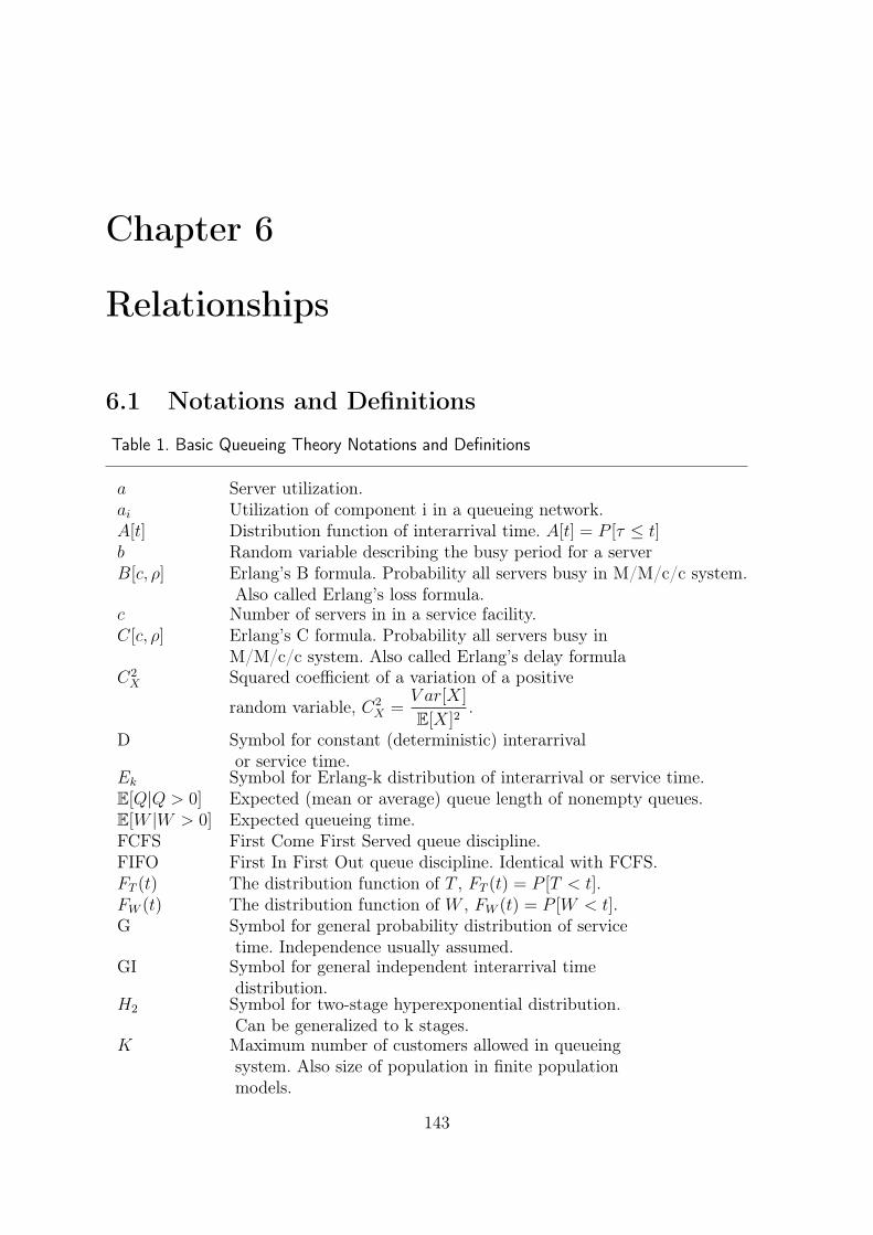
Chapter 6
Relationships
6.1 Notations and Definitions
Table 1. Basic Queueing Theory Notations and Definitions
a Server utilization.ai Utilization of component i in a queueing network.A[t] Distribution function of interarrival time. A[t] = P [τ ≤ t]b Random variable describing the busy period for a serverB[c, ρ] Erlang’s B formula. Probability all servers busy in M/M/c/c system.
Also called Erlang’s loss formula.c Number of servers in in a service facility.C[c, ρ] Erlang’s C formula. Probability all servers busy in
M/M/c/c system. Also called Erlang’s delay formulaC2X Squared coefficient of a variation of a positive
random variable, C2X =
V ar[X]
E[X]2.
D Symbol for constant (deterministic) interarrivalor service time.
Ek Symbol for Erlang-k distribution of interarrival or service time.E[Q|Q > 0] Expected (mean or average) queue length of nonempty queues.E[W |W > 0] Expected queueing time.FCFS First Come First Served queue discipline.FIFO First In First Out queue discipline. Identical with FCFS.FT (t) The distribution function of T , FT (t) = P [T < t].FW (t) The distribution function of W , FW (t) = P [W < t].G Symbol for general probability distribution of service
time. Independence usually assumed.GI Symbol for general independent interarrival time
distribution.H2 Symbol for two-stage hyperexponential distribution.
Can be generalized to k stages.K Maximum number of customers allowed in queueing
system. Also size of population in finite populationmodels.
143
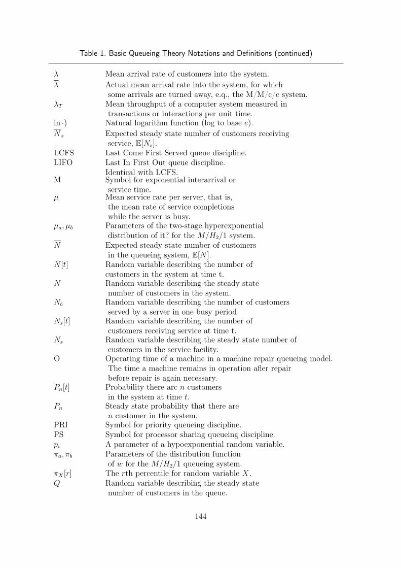
Table 1. Basic Queueing Theory Notations and Definitions (continued)
λ Mean arrival rate of customers into the system.λ Actual mean arrival rate into the system, for which
some arrivals arc turned away, e.q., the M/M/c/c system.λT Mean throughput of a computer system measured in
transactions or interactions per unit time.ln ·) Natural logarithm function (log to base e).N s Expected steady state number of customers receiving
service, E[Ns].LCFS Last Come First Served queue discipline.LIFO Last In First Out queue discipline.
Identical with LCFS.M Symbol for exponential interarrival or
service time.µ Mean service rate per server, that is,
the mean rate of service completionswhile the server is busy.
µa, µb Parameters of the two-stage hyperexponentialdistribution of it? for the M/H2/1 system.
N Expected steady state number of customersin the queueing system, E[N ].
N [t] Random variable describing the number ofcustomers in the system at time t.
N Random variable describing the steady statenumber of customers in the system.
Nb Random variable describing the number of customersserved by a server in one busy period.
Ns[t] Random variable describing the number ofcustomers receiving service at time t.
Ns Random variable describing the steady state number ofcustomers in the service facility.
O Operating time of a machine in a machine repair queueing model.The time a machine remains in operation afler repairbefore repair is again necessary.
Pn[t] Probability there arc n customersin the system at time t.
Pn Steady state probability that there aren customer in the system.
PRI Symbol for priority queueing discipline.PS Symbol for processor sharing queueing discipline.pi A parameter of a hypoexponential random variable.πa, πb Parameters of the distribution function
of w for the M/H2/1 queueing system.πX [r] The rth percentile for random variable X.Q Random variable describing the steady state
number of customers in the queue.
144
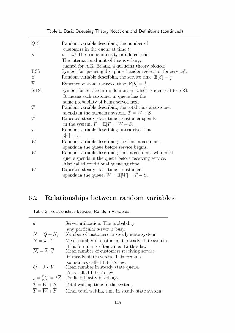
Table 1. Basic Queueing Theory Notations and Definitions (continued)
Q[t] Random variable describing the number ofcustomers in the queue at time t.
ρ ρ = λS The traffic intensity or offered load.The international unit of this is erlang,named for A.K. Erlang, a queueing theory pioneer
RSS Symbol for queueing discipline "random selection for service".S Random variable describing the service time. E[S] = 1
µ.
S Expected customer service time, E[S] = 1µ.
SIRO Symbol for service in random order, which is identical to RSS.It means each customer in queue has thesame probability of being served next.
T Random variable describing the total time a customerspends in the queueing system, T = W + S.
T Expected steady state time a customer spendsin the system, T = E[T ] = W + S.
τ Random variable describing interarrival time.E[τ ] = 1
λ.
W Random variable describing the time a customerspends in the queue before service begins.
W ′ Random variable describing time a customer who mustqueue spends in the queue before receiving service.Also called conditional queueing time.
W Expected steady state time a customerspends in the queue, W = E[W ] = T − S.
6.2 Relationships between random variables
Table 2. Relationships between Random Variables
a Server utilization. The probabilityany particular server is busy.
N = Q+Ns Number of customers in steady state system.N = λ · T Mean number of customers in steady state system.
This formula is often called Little’s law.Ns = λ · S Mean number of customers receiving service
in steady state system. This formulasometimes called Little’s law.
Q = λ ·W Mean number in steady state queue.Also called Little’s law.
ρ = E[S]E[τ ]
= λS Traffic intensity in erlangs.T = W + S Total waiting time in the system.T = W + S Mean total waiting time in steady state system.
145

146
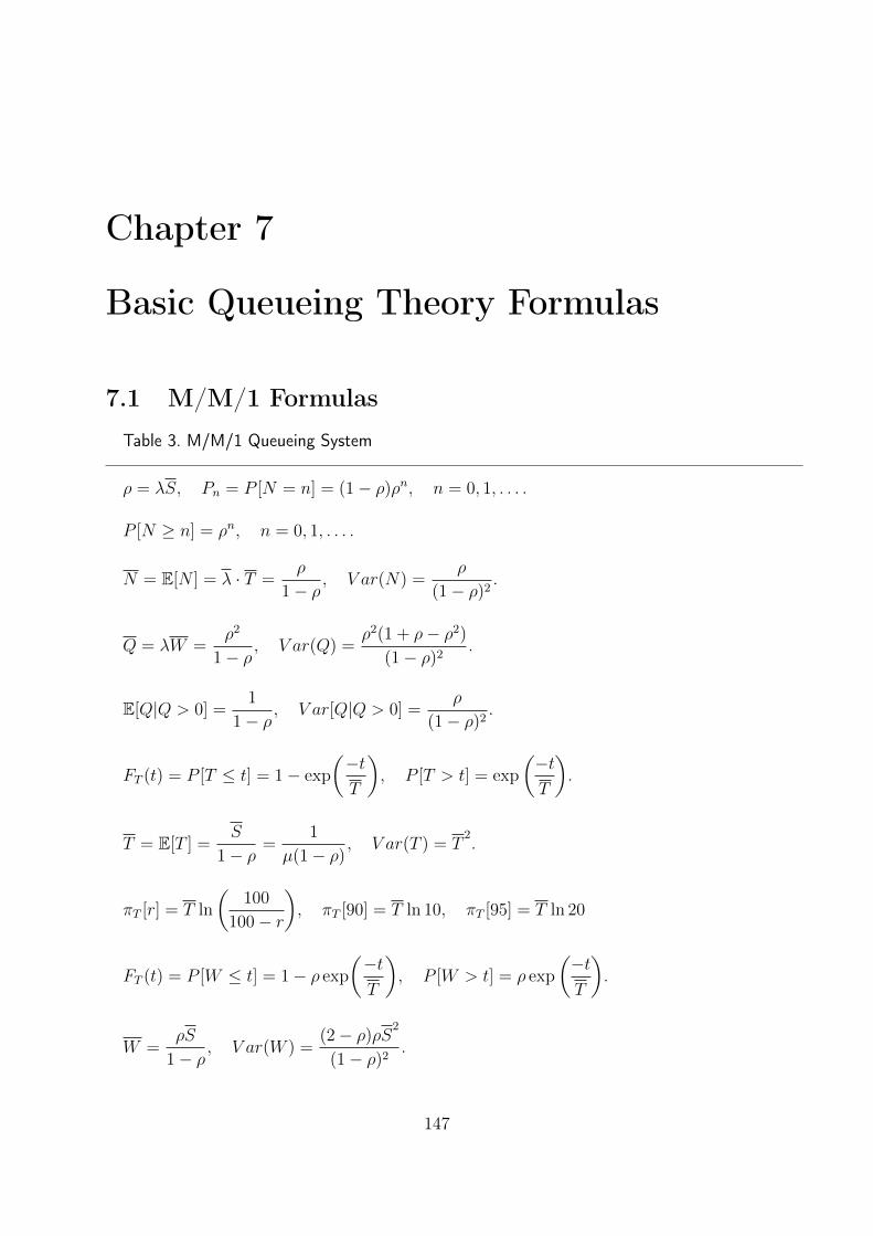
Chapter 7
Basic Queueing Theory Formulas
7.1 M/M/1 Formulas
Table 3. M/M/1 Queueing System
ρ = λS, Pn = P [N = n] = (1− ρ)ρn, n = 0, 1, . . . .
P [N ≥ n] = ρn, n = 0, 1, . . . .
N = E[N ] = λ · T =ρ
1− ρ, V ar(N) =
ρ
(1− ρ)2.
Q = λW =ρ2
1− ρ, V ar(Q) =
ρ2(1 + ρ− ρ2)
(1− ρ)2.
E[Q|Q > 0] =1
1− ρ, V ar[Q|Q > 0] =
ρ
(1− ρ)2.
FT (t) = P [T ≤ t] = 1− exp
(−tT
), P [T > t] = exp
(−tT
).
T = E[T ] =S
1− ρ=
1
µ(1− ρ), V ar(T ) = T
2.
πT [r] = T ln
(100
100− r
), πT [90] = T ln 10, πT [95] = T ln 20
FT (t) = P [W ≤ t] = 1− ρ exp
(−tT
), P [W > t] = ρ exp
(−tT
).
W =ρS
1− ρ, V ar(W ) =
(2− ρ)ρS2
(1− ρ)2.
147

πW [r] = max
{T ln
(100ρ
100− r
), 0
}.
πW [90] = max{T ln(10ρ), 0}, πW [95] = max{T ln(20ρ), 0}.
http://irh.inf.unideb.hu/user/jsztrik/education/03/EN/MM1/MM1.html
148
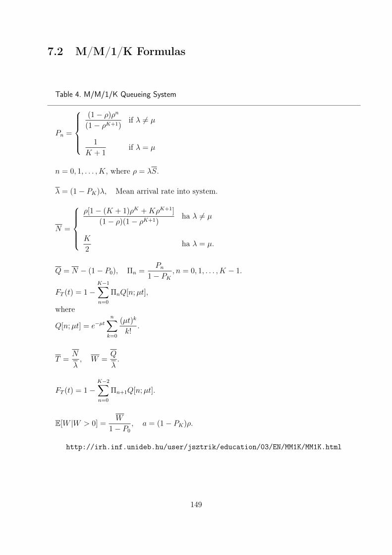
7.2 M/M/1/K Formulas
Table 4. M/M/1/K Queueing System
Pn =
(1− ρ)ρn
(1− ρK+1)if λ 6= µ
1
K + 1if λ = µ
n = 0, 1, . . . , K, where ρ = λS.
λ = (1− PK)λ, Mean arrival rate into system.
N =
ρ[1− (K + 1)ρK +KρK+1]
(1− ρ)(1− ρK+1)ha λ 6= µ
K
2ha λ = µ.
Q = N − (1− P0), Πn =Pn
1− PK, n = 0, 1, . . . , K − 1.
FT (t) = 1−K−1∑n=0
ΠnQ[n;µt],
where
Q[n;µt] = e−µtn∑k=0
(µt)k
k!.
T =N
λ, W =
Q
λ.
FT (t) = 1−K−2∑n=0
Πn+1Q[n;µt].
E[W |W > 0] =W
1− P0
, a = (1− PK)ρ.
http://irh.inf.unideb.hu/user/jsztrik/education/03/EN/MM1K/MM1K.html
149

7.3 M/M/c Formulas
Table 5. M/M/c Queueing System
ρ = λS, a =ρ
c
P0 =
[c−1∑n=0
ρn
n!+
ρc
c!(1− a)
]−1
=c!(1− a)P [N ≥ c]
ρc.
Pn =
ρn
n!P0, if n ≤ c
ρn
c!cn−cP0, if n ≥ c.
P [N ≥ n] =
P0
[c−1∑k=n
ρk
k!+
ρc
c!(1− a)
]if n < c,
P0
[acan−c
c!(1− a)
]= P [N ≥ c]an−c if n ≥ c
Q = λ ·W =ρP [N ≥ c]
c(1− a),
where
P [N ≥ c] = C[c, ρ] =
ρc
c!
(1− ρ
c)c−1∑n=0
ρn
n!+ρc
c!
.
V ar(Q) =aC[c, ρ][1 + a− aC[c, ρ]]
(1− a)2.
N = λ · T = Q+ ρ.
V ar(N) = V ar(Q) + ρ(1 + P [N ≥ c]).
W [0] = 1− P [N ≥ c], FT (t) = 1− P [N ≥ c] exp[−cµt(1− a)],
W =P [N ≥ c]S
c(1− a).
150

Table 5. M/M/c Queueing System (continued)
V ar(W ) =[2− C[c, ρ]]C[c, ρ]S
2
c2(1− a)2.
πW [r] = max{0, S
c(1− a)ln
(100C[c, ρ]
100− r
)}.
πW [90] = max{0, S
c(1− a)ln(10C[c, ρ])}.
πW [95] = max{0, S
c(1− a)ln(20C[c, ρ])}.
WW ′ = P [W ≤ t|W > 0] = 1− exp
(−ct(1− a)
S
), t > 0.
E[W |W > 0] = E[W ′] =S
c(1− a).
V ar([W |W > 0] =
(S
c(1− a)
)2
.
FT (t) =
1 + C1e−µt + C2e
−cµt(1−a) if ρ 6= c− 1
1− {1 + C[c, ρ]µt}e−µt if ρ = c− 1
where
C1 =P [N ≥ c]
1− c(1− a)− 1,
and
C2 =P [N ≥ c]
c(1− a)− 1.
T = W + S.
E[T 2] =
2P [N ≥ c][1− c2(1− a)2]S
2
(ρ+ 1− c)c2(1− a)2+ 2S
2 if ρ 6= c− 1
2{2P [N ≥ c] + 1}S2 if ρ = c− 1
V ar(T ) = E[T 2]− T 2.
πT [90] ≈ T + 1.3D(T ), πT [95] ≈ T + 2D(T ) (estimates due to James Martin).
http://irh.inf.unideb.hu/user/jsztrik/education/03/EN/MMc/MMc.html
151

7.4 M/M/2 Formulas
Table 6. M/M/2 Queueing System
ρ = λS, a =ρ
2
P0 =1− a1 + a
.
Pn = 2P0an, n = 1, 2, 3, . . .
P [N ≥ n] =2an
1 + a, n = 1, 2, . . .
Q = λW =2a3
1− a2,
P [N ≥ 2] = C[2, ρ] is the probability that ail arriving customermust queue for service. P [N ≥ 2] is given by
P [N ≥ 2] = C[2, ρ] =2a2
1 + a.
V ar(Q) =2a3[(1 + a)2 − 2a3]
(1− a2)2.
N = λ · T = Q+ ρ =2a
1− a2.
V ar(N) = V ar(Q) +2a(1 + a+ 2a2)
1 + a.
W [0] =1 + a− 2a2
1 + a.
FT (t) = 1− 2a2
1 + aexp[−2µt(1− a)]
W =a2S
1− a2.
V ar(W ) =a2(1 + a− a2)S
2
(1− a2)2.
πW [r] = max{0, S
2(1− a)ln
(200a2
(100− r)(1 + a)
)}.
152
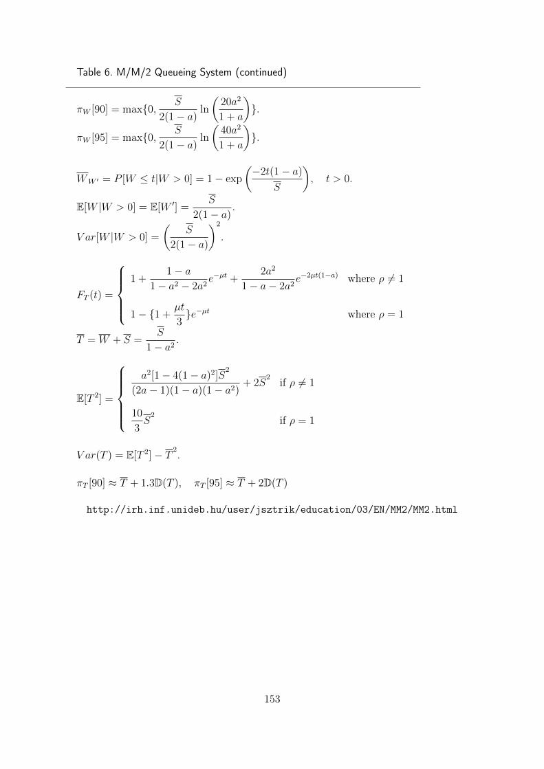
Table 6. M/M/2 Queueing System (continued)
πW [90] = max{0, S
2(1− a)ln
(20a2
1 + a
)}.
πW [95] = max{0, S
2(1− a)ln
(40a2
1 + a
)}.
WW ′ = P [W ≤ t|W > 0] = 1− exp
(−2t(1− a)
S
), t > 0.
E[W |W > 0] = E[W ′] =S
2(1− a).
V ar[W |W > 0] =
(S
2(1− a)
)2
.
FT (t) =
1 +
1− a1− a2 − 2a2
e−µt +2a2
1− a− 2a2e−2µt(1−a) where ρ 6= 1
1− {1 +µt
3}e−µt where ρ = 1
T = W + S =S
1− a2.
E[T 2] =
a2[1− 4(1− a)2]S
2
(2a− 1)(1− a)(1− a2)+ 2S
2 if ρ 6= 1
10
3S
2 if ρ = 1
V ar(T ) = E[T 2]− T 2.
πT [90] ≈ T + 1.3D(T ), πT [95] ≈ T + 2D(T )
http://irh.inf.unideb.hu/user/jsztrik/education/03/EN/MM2/MM2.html
153
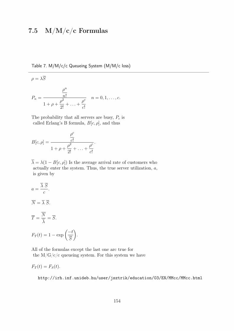
7.5 M/M/c/c Formulas
Table 7. M/M/c/c Queueing System (M/M/c loss)
ρ = λS
Pn =
ρn
n!
1 + ρ+ρ2
2!+ . . .+
ρc
c!
n = 0, 1, . . . , c.
The probability that all servers are busy, Pc iscalled Erlang’s B formula, B[c, ρ], and thus
B[c, ρ] =
ρc
c!
1 + ρ+ρ2
2!+ . . .+
ρc
c!
.
λ = λ(1−B[c, ρ]) Is the average arrival rate of customers whoactually enter the system. Thus, the true server utilization, a,is given by
a =λ S
c.
N = λ S.
T =N
λ= S.
FT (t) = 1− exp
(−tS
).
All of the formulas except the last one arc true forthe M/G/c/c queueing system. For this system we have
FT (t) = FS(t).
http://irh.inf.unideb.hu/user/jsztrik/education/03/EN/MMcc/MMcc.html
154

7.6 M/M/c/K Formulas
Table 8. M/M/c/K Queueing System
ρ = λS.
P0 =
[c∑
n=0
ρn
n!+ρc
c!
K−c∑n=1
(ρ
c
)n]−1
.
Pn =
ρn
n!P0 if n = 1, 2, . . . , c,
ρn
c!
(ρc
)n−cP0 if n = c+ 1, . . . , K.
The average arrival rate of customers who actuallyenter the system is λ = λ(1− PK).
The actual mean server utilization, a, is given by:
a =λ S
c.
Q =ρcrP0
c!(1− r)2
[1 + (K − c)rK−c+1 − (K − c+ 1)rK−c
],
where
r =ρ
c.
N = Q+ E[Ns] = Q+c−1∑n=0
nPn + c
(1−
c−1∑n=0
Pn
).
By Little’s Law
W =Q
λ, T =
N
λ.
Πn =Pn
1− PK, n = 0, 1, 2, . . . , K − 1,
155
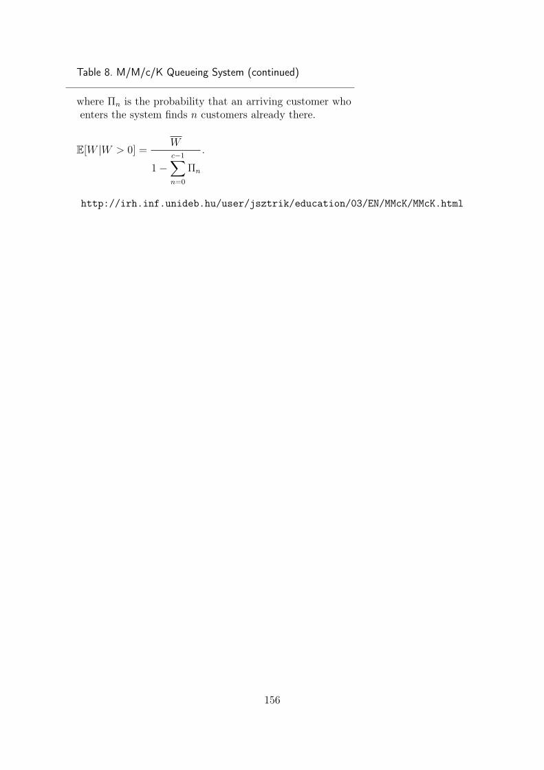
Table 8. M/M/c/K Queueing System (continued)
where Πn is the probability that an arriving customer whoenters the system finds n customers already there.
E[W |W > 0] =W
1−c−1∑n=0
Πn
.
http://irh.inf.unideb.hu/user/jsztrik/education/03/EN/MMcK/MMcK.html
156
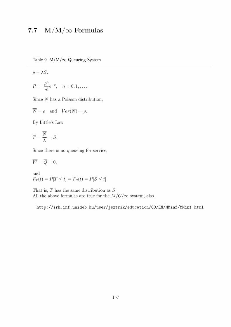
7.7 M/M/∞ Formulas
Table 9. M/M/∞ Queueing System
ρ = λS.
Pn =ρn
n!e−ρ, n = 0, 1, . . . .
Since N has a Poisson distribution,
N = ρ and V ar(N) = ρ.
By Little’s Law
T =N
λ= S.
Since there is no queueing for service,
W = Q = 0,
andFT (t) = P [T ≤ t] = FS(t) = P [S ≤ t]
That is, T has the same distribution as S.All the above formulas arc true for the M/G/∞ system, also.
http://irh.inf.unideb.hu/user/jsztrik/education/03/EN/MMinf/MMinf.html
157
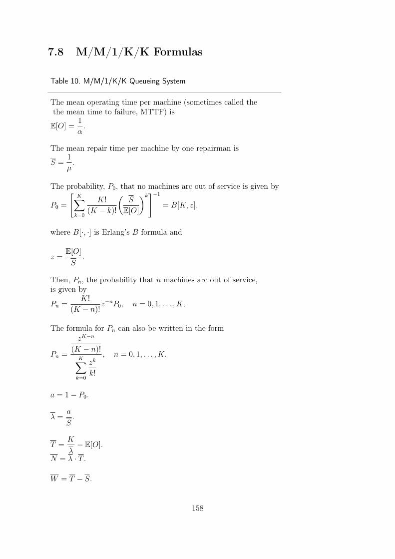
7.8 M/M/1/K/K Formulas
Table 10. M/M/1/K/K Queueing System
The mean operating time per machine (sometimes called thethe mean time to failure, MTTF) is
E[O] =1
α.
The mean repair time per machine by one repairman is
S =1
µ.
The probability, P0, that no machines arc out of service is given by
P0 =
[K∑k=0
K!
(K − k)!
(S
E[O]
)k]−1
= B[K, z],
where B[·, ·] is Erlang’s B formula and
z =E[O]
S.
Then, Pn, the probability that n machines arc out of service,is given by
Pn =K!
(K − n)!z−nP0, n = 0, 1, . . . , K,
The formula for Pn can also be written in the form
Pn =
zK−n
(K − n)!K∑k=0
zk
k!
, n = 0, 1, . . . , K.
a = 1− P0.
λ =a
S.
T =K
λ− E[O].
N = λ · T .
W = T − S.
158

Table 10. M/M/1/K/K Queueing System (continued)
Πn =(K − n)Pn
K −N=
zK−n−1
(K − n− 1)!K−1∑k=0
zk
k!
, n = 0, 1, 2, . . . , K − 1,
where Πn is the probability that a machine that breaks downfinds n machines in the repair facility.
FT (t) = P [T ≤ t] = 1− Q(K − 1; z + tµ)
Q(K − 1; z), t ≥ 0,
where
Q(n;x) = e−xn∑k=0
xk
k!.
FT (t) = P [W ≤ t] = 1− Q(K − 2; z + tµ)
Q(K − 1; z), t ≥ 0,
E[W |W > 0] =W
1− Π0
.
http://irh.inf.unideb.hu/user/jsztrik/education/03/EN/MM1KK/MM1KK.html
159
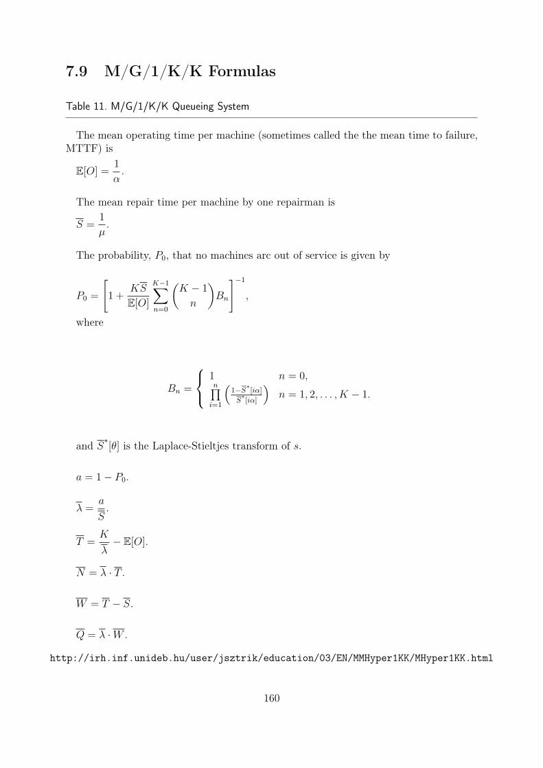
7.9 M/G/1/K/K Formulas
Table 11. M/G/1/K/K Queueing System
The mean operating time per machine (sometimes called the the mean time to failure,MTTF) is
E[O] =1
α.
The mean repair time per machine by one repairman is
S =1
µ.
The probability, P0, that no machines arc out of service is given by
P0 =
[1 +
KS
E[O]
K−1∑n=0
(K − 1
n
)Bn
]−1
,
where
Bn =
1 n = 0,n∏i=1
(1−S∗[iα]
S∗[iα]
)n = 1, 2, . . . , K − 1.
and S∗[θ] is the Laplace-Stieltjes transform of s.
a = 1− P0.
λ =a
S.
T =K
λ− E[O].
N = λ · T .
W = T − S.
Q = λ ·W .
http://irh.inf.unideb.hu/user/jsztrik/education/03/EN/MMHyper1KK/MHyper1KK.html
160
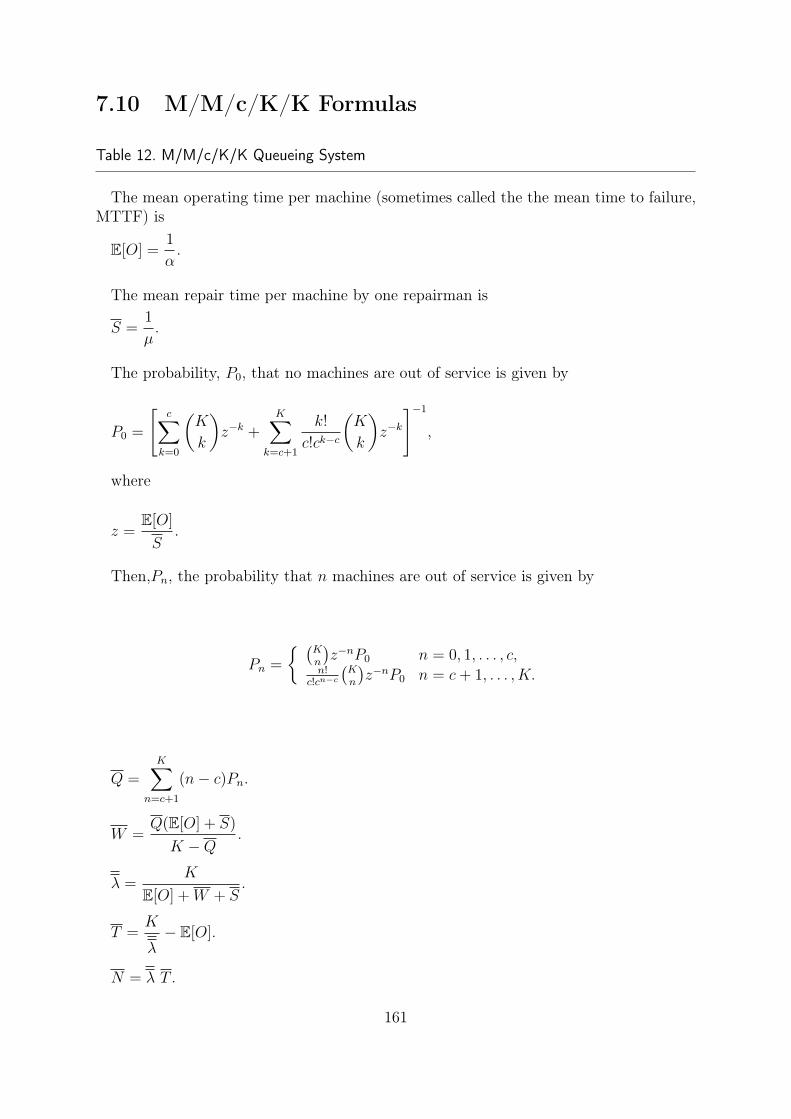
7.10 M/M/c/K/K Formulas
Table 12. M/M/c/K/K Queueing System
The mean operating time per machine (sometimes called the the mean time to failure,MTTF) is
E[O] =1
α.
The mean repair time per machine by one repairman is
S =1
µ.
The probability, P0, that no machines are out of service is given by
P0 =
[c∑
k=0
(K
k
)z−k +
K∑k=c+1
k!
c!ck−c
(K
k
)z−k
]−1
,
where
z =E[O]
S.
Then,Pn, the probability that n machines are out of service is given by
Pn =
{ (Kn
)z−nP0 n = 0, 1, . . . , c,
n!c!cn−c
(Kn
)z−nP0 n = c+ 1, . . . , K.
Q =K∑
n=c+1
(n− c)Pn.
W =Q(E[O] + S)
K −Q.
λ =K
E[O] +W + S.
T =K
λ− E[O].
N = λ T .
161

Table 12. M/M/c/K/K Queueing System (continued)
Πn =(K − n)Pn
K −N,
where Πn is the probability that a machine which breaks down finds n inoperable ma-chines already in the repair facility. We denote Πn by Πn[K] to emphasize the fact thatthere are K machines. It can be shown that
Πn[K] = Pn[K − 1], n = 0, 1, . . . , K − 1.
Pn[K − 1] =cc
c!
p(K − n− 1; cz)
p(K − 1; cz)P0[K − 1],
where, of course,
p(k;α) =αk
k!e−α.
FT (t) = P [W ≤ t] = 1− ccQ(K − c− 1; cz)P0[K − 1]
c!p(K − 1; cz), t ≥ 0,
where
Q(k;α) = e−αk∑
n=0
αn
n!.
FT (t) = P [T ≤ t] = 1− C1 exp(−t/S) + C2Q(K − c− 1; c(z + tµ))
Q(K − c− 1; cz),
t ≥ 0,
where C1 = 1 + C2 �s
C2 =ccQ(K − c− 1; cz)
c!(c− 1)(K − c− 1)!p(K − 1; cz)P0[K − 1].
The probability that a machine that breaks down must wait for repair is given by
D =K−1∑n=c
Πn = 1−c−1∑n=0
Πn.
E[W |W > 0] =W
D.
http://irh.inf.unideb.hu/user/jsztrik/education/03/EN/MMcKK/MMcKK.html
162
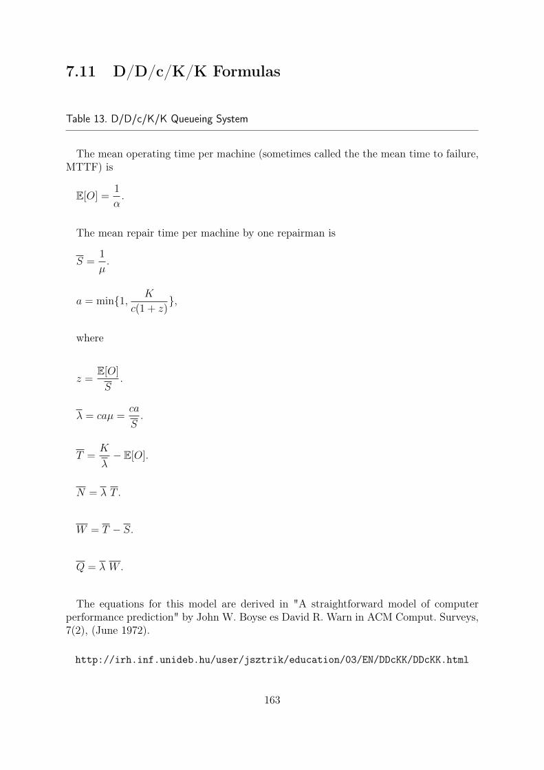
7.11 D/D/c/K/K Formulas
Table 13. D/D/c/K/K Queueing System
The mean operating time per machine (sometimes called the the mean time to failure,MTTF) is
E[O] =1
α.
The mean repair time per machine by one repairman is
S =1
µ.
a = min{1, K
c(1 + z)},
where
z =E[O]
S.
λ = caµ =ca
S.
T =K
λ− E[O].
N = λ T .
W = T − S.
Q = λ W .
The equations for this model are derived in "A straightforward model of computerperformance prediction" by John W. Boyse es David R. Warn in ACM Comput. Surveys,7(2), (June 1972).
http://irh.inf.unideb.hu/user/jsztrik/education/03/EN/DDcKK/DDcKK.html
163

7.12 M/G/1 Formulas
Table 14. M/G/1 Queueing System
The z-transform of N , the steady-state number of customers in the system is given by:
GN(z) =∞∑n=0
Pnzn =
(1− ρ)(1− z)S∗[λ(1− z)]
S∗[λ(1− z)]− z
,
where S∗ is the Laplace-Stieltjes transform of the servide time S. The Laplace-Stieltjestransforms of T and W are given by
W ∗[θ] =(1− ρ)θS
∗[θ]
θ − λ+ λS∗[θ]
,
�s
W∗[θ] =
(1− ρ)θ
θ − λ+ λS∗[θ]
.
Each of the three transforms above is called the Pollaczek-Khintchine transform equa-tion by various authors. The probability, P0, of no customers in the system has the simpleand intuitive equation P0 = 1 − ρ, where the server utilization ρ = λS. The probabilitythat the server is busy is P [N ≥ 1] = ρ.
W =λE[S2]
2(1− ρ)=
ρS
1− ρ
(1 + C2
S
2
)(Pollaczek formula).
Q = λW .
V ar(Q) =λ3E[S3]
3(1− ρ)+
(λ2E[S2]
2(1− ρ)
)2
+λ2E[S2]
2(1− ρ).
E[W |W > 0] =S
1− ρ
(1 + C2
S
2
).
E[W 2] = 2W2
+λE[S3]
3(1− ρ).
V ar(W ) = E[W 2]−W 2.
T = W + S.
N = λ · T = Q+ ρ.
V ar(N) =λ3E[S3]
3(1− ρ)+
(λ2E[S2]
2(1− ρ)
)2
+λ2(3− 2ρ)E[S2]
2(1− ρ)+ ρ(1− ρ).
E[T 2] = E[W 2] +E[S2]
1− ρ.
164
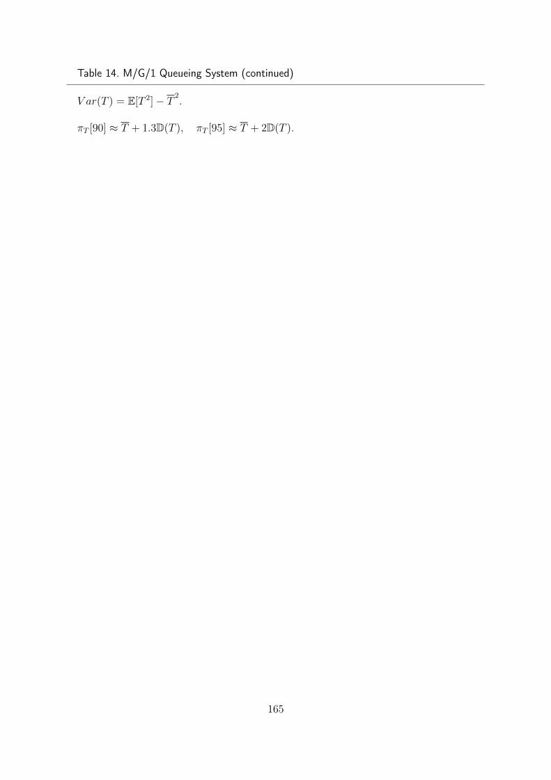
Table 14. M/G/1 Queueing System (continued)
V ar(T ) = E[T 2]− T 2.
πT [90] ≈ T + 1.3D(T ), πT [95] ≈ T + 2D(T ).
165
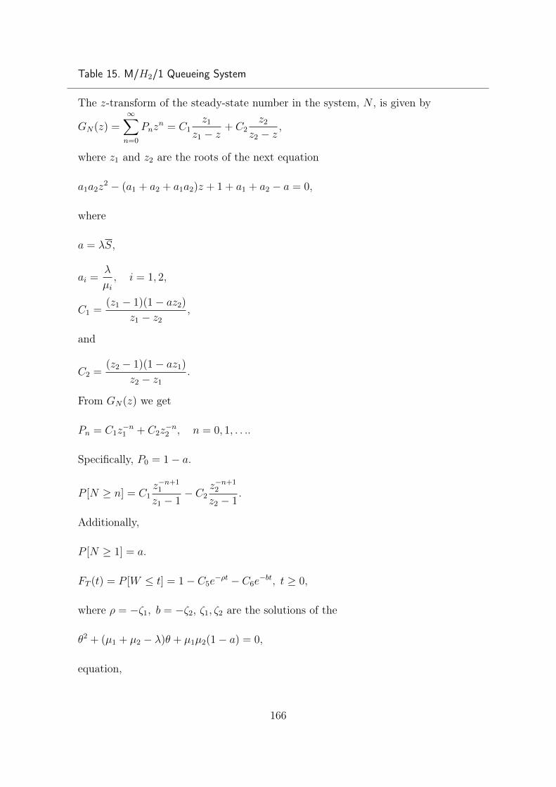
Table 15. M/H2/1 Queueing System
The z-transform of the steady-state number in the system, N , is given by
GN(z) =∞∑n=0
Pnzn = C1
z1
z1 − z+ C2
z2
z2 − z,
where z1 and z2 are the roots of the next equation
a1a2z2 − (a1 + a2 + a1a2)z + 1 + a1 + a2 − a = 0,
where
a = λS,
ai =λ
µi, i = 1, 2,
C1 =(z1 − 1)(1− az2)
z1 − z2
,
and
C2 =(z2 − 1)(1− az1)
z2 − z1
.
From GN(z) we get
Pn = C1z−n1 + C2z
−n2 , n = 0, 1, . . ..
Specifically, P0 = 1− a.
P [N ≥ n] = C1z−n+1
1
z1 − 1− C2
z−n+12
z2 − 1.
Additionally,
P [N ≥ 1] = a.
FT (t) = P [W ≤ t] = 1− C5e−ρt − C6e
−bt, t ≥ 0,
where ρ = −ζ1, b = −ζ2, ζ1, ζ2 are the solutions of the
θ2 + (µ1 + µ2 − λ)θ + µ1µ2(1− a) = 0,
equation,
166

Table 15. M/H2/1 Queueing System (continued)
C5 =λ(1− a)ζ1 + a(1− a)µ1µ2
ρ(ζ1 − ζ2)
and
C6 =λ(1− a)ζ2 + a(1− a)µ1µ2
ρ(ζ2 − ζ1).
W =λE[S2]
2(1− a)=
aS
1− a
(1 + C2
S
2
). (Pollaczek-formula)
E[W |W > 0] =S
1− a
(1 + C2
S
2
).
E[W 2] = 2W2
+λE[S3]
3(1− a).
In this formula we substitute
E[S3] =6p1
µ31
+6p2
µ32
,
then
V ar(W ) = E[W 2]−W 2.
FT (t) = P [T ≤ t] = 1− πae−µat − πbe−µbt, t ≥ 0,
where
πa = C1z1
z1 − 1,
πb = C2z2
z2 − 1,
167
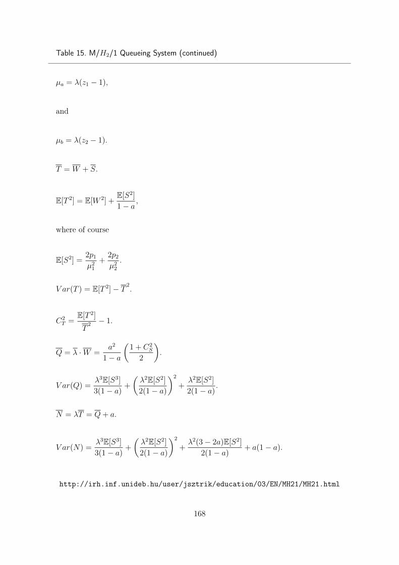
Table 15. M/H2/1 Queueing System (continued)
µa = λ(z1 − 1),
and
µb = λ(z2 − 1).
T = W + S.
E[T 2] = E[W 2] +E[S2]
1− a,
where of course
E[S2] =2p1
µ21
+2p2
µ22
.
V ar(T ) = E[T 2]− T 2.
C2T =
E[T 2]
T2 − 1.
Q = λ ·W =a2
1− a
(1 + C2
S
2
).
V ar(Q) =λ3E[S3]
3(1− a)+
(λ2E[S2]
2(1− a)
)2
+λ2E[S2]
2(1− a).
N = λT = Q+ a.
V ar(N) =λ3E[S3]
3(1− a)+
(λ2E[S2]
2(1− a)
)2
+λ2(3− 2a)E[S2]
2(1− a)+ a(1− a).
http://irh.inf.unideb.hu/user/jsztrik/education/03/EN/MH21/MH21.html
168

Table 16. M/Gamma/1 Queueing System
Since S has Gamma-distribution
E[Sn] =β(β + 1) . . . (β + n− 1)
αn, n = 1, 2, . . ..
Since
C2S =
1
β,
so
E[S2] = S2(1 + C2
S),
E[S3] = S3(1 + C2
S)(1 + 2C2S),
and
E[sn] = Snn−1∏k=1
(1 + kC2S), n = 1, 2, . . ..
This time
W =λE[S2]
2(1− a)=
aS
1− a
(1 + C2
S
2
),
Q = λ ·W ,
V ar(Q) =a2(1 + C2
S)
2(1− a)
[1 +
a2(1 + C2S)
2(1− a)+
2a(1 + 2C2S)
3
],
E[W |W > 0] =S
1− a
(1 + C2
S
2
),
E[W 2] = 2W2
+aS
2(1 + C2
S)(1 + 2C2S)
3(1− a),
V ar(W ) = E[W 2]−W 2,
T = W + S, N = λ · T = Q+ a,
V ar(N) =a3(1 + C2
S)(1 + 2C2S)
3(1− a)+
(a2(1 + C2
S)
2(1− a)
)2
+a2(3− 2a)(1 + C2
S)
2(1− a)+ a(1− a).
E[T 2] = E[W 2] +S
2(1 + C2
S)
1− a.
V ar(T ) = E[T 2]− T 2.
πT [90] ≈ T + 1.3D(T ), πT [95] ≈ T + 2D(T ).
http://irh.inf.unideb.hu/user/jsztrik/education/03/EN/MGamma1/MGamma1.html
169
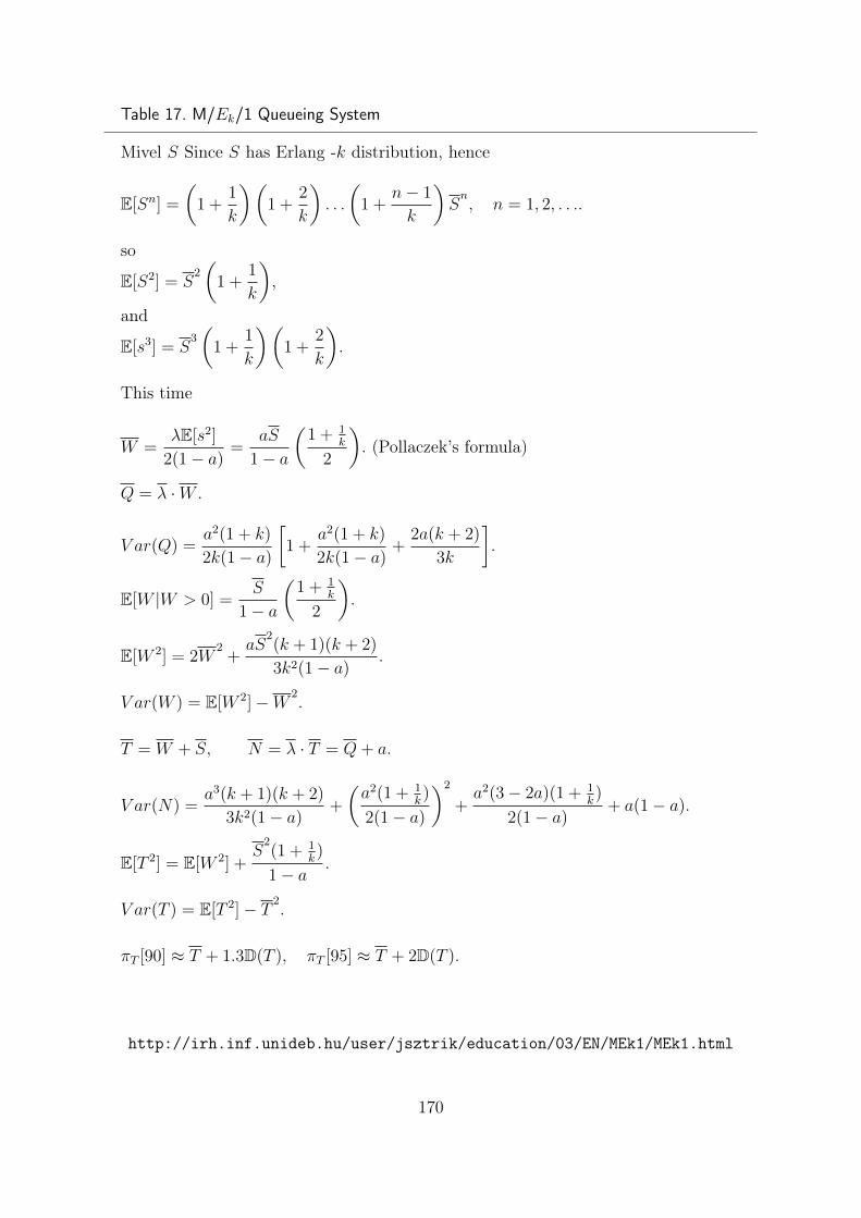
Table 17. M/Ek/1 Queueing System
Mivel S Since S has Erlang -k distribution, hence
E[Sn] =
(1 +
1
k
)(1 +
2
k
). . .
(1 +
n− 1
k
)Sn, n = 1, 2, . . ..
so
E[S2] = S2(
1 +1
k
),
and
E[s3] = S3(
1 +1
k
)(1 +
2
k
).
This time
W =λE[s2]
2(1− a)=
aS
1− a
(1 + 1
k
2
). (Pollaczek’s formula)
Q = λ ·W .
V ar(Q) =a2(1 + k)
2k(1− a)
[1 +
a2(1 + k)
2k(1− a)+
2a(k + 2)
3k
].
E[W |W > 0] =S
1− a
(1 + 1
k
2
).
E[W 2] = 2W2
+aS
2(k + 1)(k + 2)
3k2(1− a).
V ar(W ) = E[W 2]−W 2.
T = W + S, N = λ · T = Q+ a.
V ar(N) =a3(k + 1)(k + 2)
3k2(1− a)+
(a2(1 + 1
k)
2(1− a)
)2
+a2(3− 2a)(1 + 1
k)
2(1− a)+ a(1− a).
E[T 2] = E[W 2] +S
2(1 + 1
k)
1− a.
V ar(T ) = E[T 2]− T 2.
πT [90] ≈ T + 1.3D(T ), πT [95] ≈ T + 2D(T ).
http://irh.inf.unideb.hu/user/jsztrik/education/03/EN/MEk1/MEk1.html
170

Table 18. M/D/1 Queueing System
Since S has a constant distribution
E[Sn] = Sn, n = 1, 2, . . .,
so
GN(z) =(1− a)(1− z)
1− zea(1−z) .
We suppose that
|zea(1−z)| < 1,
we can expand GN(z) in the geometric series
gN(z) = (1− a)(1− z)∞∑j=0
[zea(1−z)]j.
This thime we can show that,
P1 = (1− a)(ea − 1),
and
Pn = (1− a)n∑j=1
(−1)n−j(ja)n−j−1(ja+ n− j)eja
(n− j)!n = 2, 3, . . ..
Additionally
FT (t) =k−1∑n=0
Pn + Pk
(t− (k − 1)S
S
),
where (k − 1)S ≤ t ≤ kS, k = 1, 2, . . ..
171
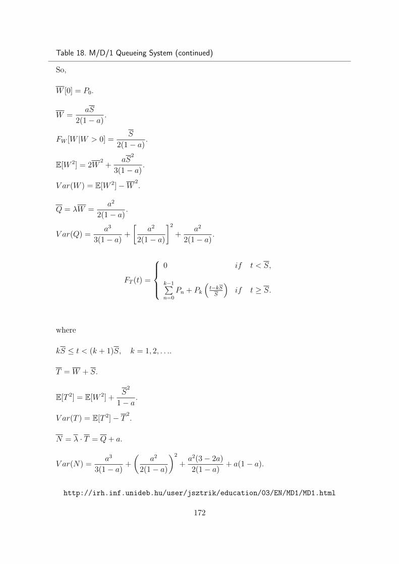
Table 18. M/D/1 Queueing System (continued)
So,
W [0] = P0.
W =aS
2(1− a).
FW [W |W > 0] =S
2(1− a).
E[W 2] = 2W2
+aS
2
3(1− a).
V ar(W ) = E[W 2]−W 2.
Q = λW =a2
2(1− a).
V ar(Q) =a3
3(1− a)+
[a2
2(1− a)
]2
+a2
2(1− a).
FT (t) =
0 if t < S,
k−1∑n=0
Pn + Pk
(t−kSS
)if t ≥ S.
where
kS ≤ t < (k + 1)S, k = 1, 2, . . ..
T = W + S.
E[T 2] = E[W 2] +S
2
1− a.
V ar(T ) = E[T 2]− T 2.
N = λ · T = Q+ a.
V ar(N) =a3
3(1− a)+
(a2
2(1− a)
)2
+a2(3− 2a)
2(1− a)+ a(1− a).
http://irh.inf.unideb.hu/user/jsztrik/education/03/EN/MD1/MD1.html
172
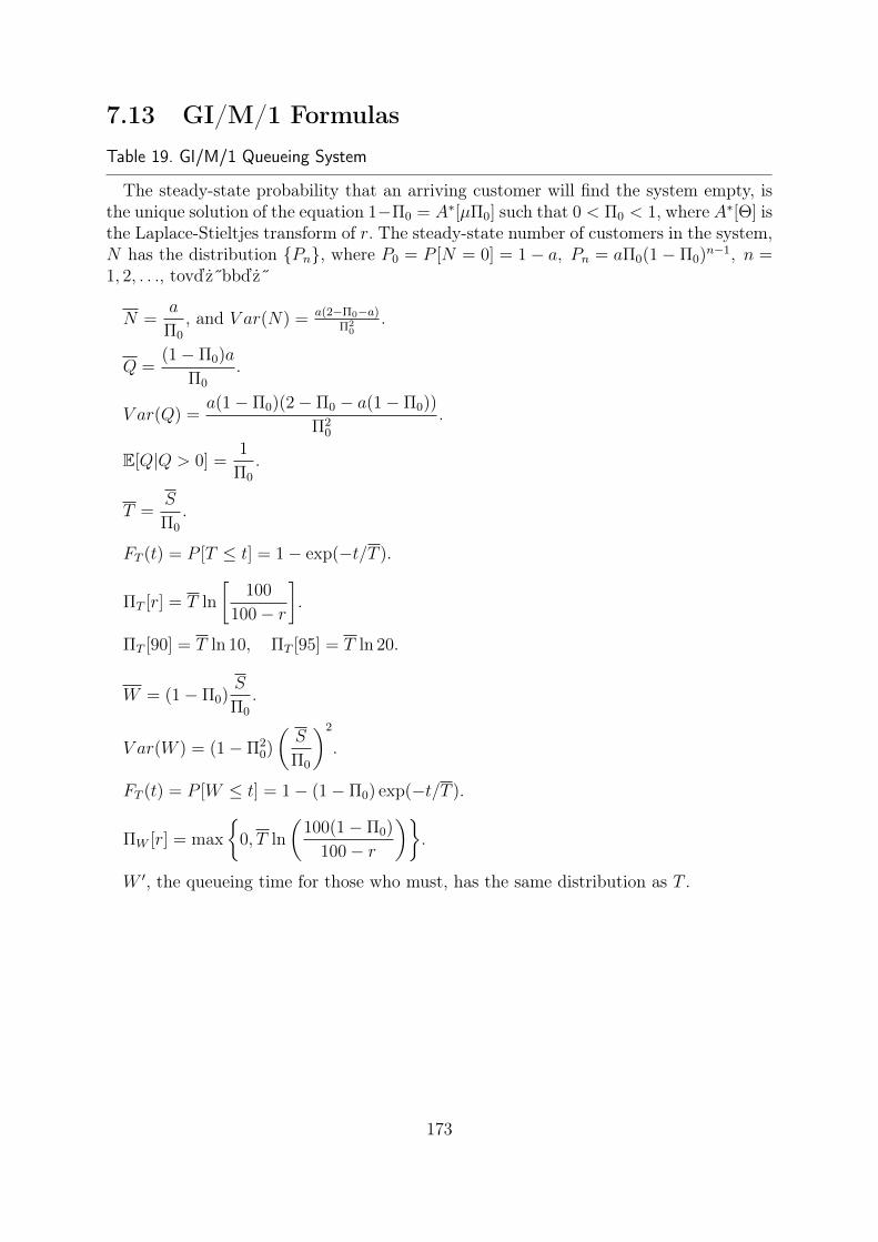
7.13 GI/M/1 FormulasTable 19. GI/M/1 Queueing System
The steady-state probability that an arriving customer will find the system empty, isthe unique solution of the equation 1−Π0 = A∗[µΠ0] such that 0 < Π0 < 1, where A∗[Θ] isthe Laplace-Stieltjes transform of r. The steady-state number of customers in the system,N has the distribution {Pn}, where P0 = P [N = 0] = 1− a, Pn = aΠ0(1− Π0)n−1, n =1, 2, . . ., tovďż˝bbďż˝
N =a
Π0
, and V ar(N) = a(2−Π0−a)
Π20
.
Q =(1− Π0)a
Π0
.
V ar(Q) =a(1− Π0)(2− Π0 − a(1− Π0))
Π20
.
E[Q|Q > 0] =1
Π0
.
T =S
Π0
.
FT (t) = P [T ≤ t] = 1− exp(−t/T ).
ΠT [r] = T ln
[100
100− r
].
ΠT [90] = T ln 10, ΠT [95] = T ln 20.
W = (1− Π0)S
Π0
.
V ar(W ) = (1− Π20)
(S
Π0
)2
.
FT (t) = P [W ≤ t] = 1− (1− Π0) exp(−t/T ).
ΠW [r] = max
{0, T ln
(100(1− Π0)
100− r
)}.
W ′, the queueing time for those who must, has the same distribution as T .
173

Table 20. Π0 versus a for GI/M/1 Queueing System 1
a E2 E3 U D H2 H2
0.100 0.970820 0.987344 0.947214 0.999955 0.815535 0.8105750.200 0.906226 0.940970 0.887316 0.993023 0.662348 0.6244040.300 0.821954 0.868115 0.817247 0.959118 0.536805 0.4449490.400 0.724695 0.776051 0.734687 0.892645 0.432456 0.2812650.500 0.618034 0.669467 0.639232 0.796812 0.343070 0.1543030.600 0.504159 0.551451 0.531597 0.675757 0.263941 0.0812650.700 0.384523 0.626137 0.412839 0.533004 0.191856 0.0449490.800 0.260147 0.289066 0.284028 0.371370 0.124695 0.0244040.900 0.131782 0.147390 0.146133 0.193100 0.061057 0.0104950.950 0.066288 0.074362 0.074048 0.098305 0.030252 0.0049990.980 0.026607 0.029899 0.029849 0.039732 0.012039 0.0019410.999 0.001333 0.001500 0.001500 0.001999 0.000600 0.000095
http://irh.inf.unideb.hu/user/jsztrik/education/03/EN/GIM1/GIM1.html
1At the first H2 distribution p1 = 0.4, µ1 = 0.5λ, µ2 = 3λ. At the second H2 distribution p1 =0.024405, µ1 = 2p1λ, ďż˝s µ2 = 2p2λ.
174
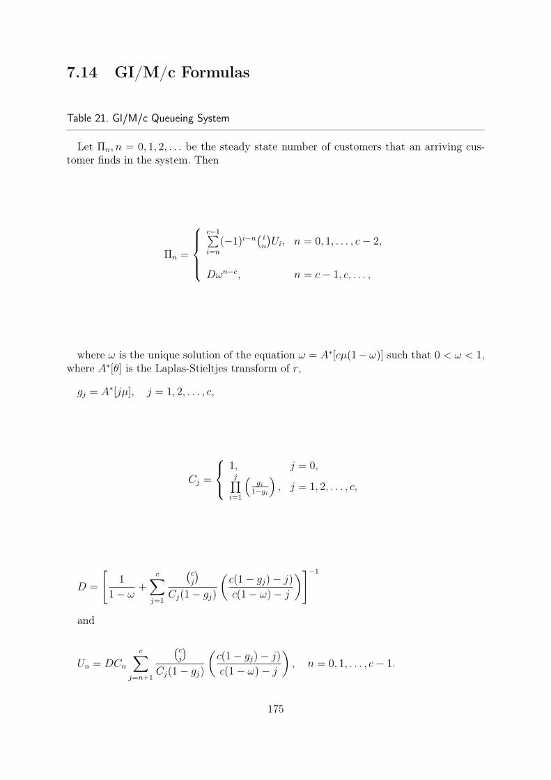
7.14 GI/M/c Formulas
Table 21. GI/M/c Queueing System
Let Πn, n = 0, 1, 2, . . . be the steady state number of customers that an arriving cus-tomer finds in the system. Then
Πn =
c−1∑i=n
(−1)i−n(in
)Ui, n = 0, 1, . . . , c− 2,
Dωn−c, n = c− 1, c, . . . ,
where ω is the unique solution of the equation ω = A∗[cµ(1− ω)] such that 0 < ω < 1,where A∗[θ] is the Laplas-Stieltjes transform of r,
gj = A∗[jµ], j = 1, 2, . . . , c,
Cj =
1, j = 0,j∏i=1
(gi
1−gi
), j = 1, 2, . . . , c,
D =
[1
1− ω+
c∑j=1
(cj
)Cj(1− gj)
(c(1− gj)− j)c(1− ω)− j
)]−1
and
Un = DCn
c∑j=n+1
(cj
)Cj(1− gj)
(c(1− gj)− j)c(1− ω)− j
), n = 0, 1, . . . , c− 1.
175
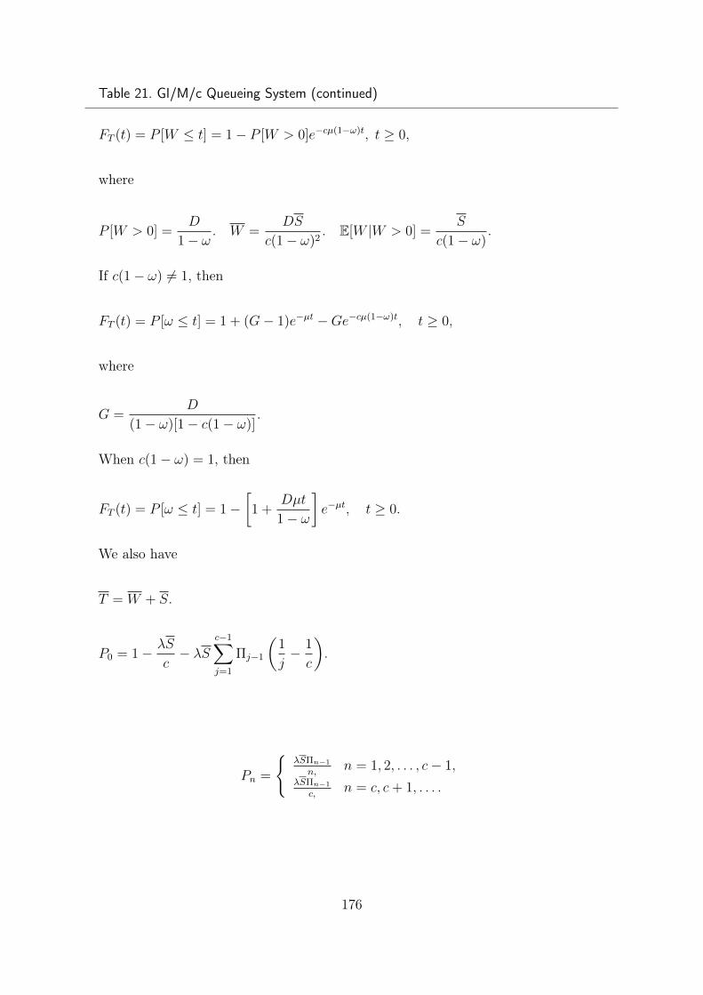
Table 21. GI/M/c Queueing System (continued)
FT (t) = P [W ≤ t] = 1− P [W > 0]e−cµ(1−ω)t, t ≥ 0,
where
P [W > 0] =D
1− ω. W =
DS
c(1− ω)2. E[W |W > 0] =
S
c(1− ω).
If c(1− ω) 6= 1, then
FT (t) = P [ω ≤ t] = 1 + (G− 1)e−µt −Ge−cµ(1−ω)t, t ≥ 0,
where
G =D
(1− ω)[1− c(1− ω)].
When c(1− ω) = 1, then
FT (t) = P [ω ≤ t] = 1−[1 +
Dµt
1− ω
]e−µt, t ≥ 0.
We also have
T = W + S.
P0 = 1− λS
c− λS
c−1∑j=1
Πj−1
(1
j− 1
c
).
Pn =
{λSΠn−1
n,n = 1, 2, . . . , c− 1,
λSΠn−1
c,n = c, c+ 1, . . . .
176
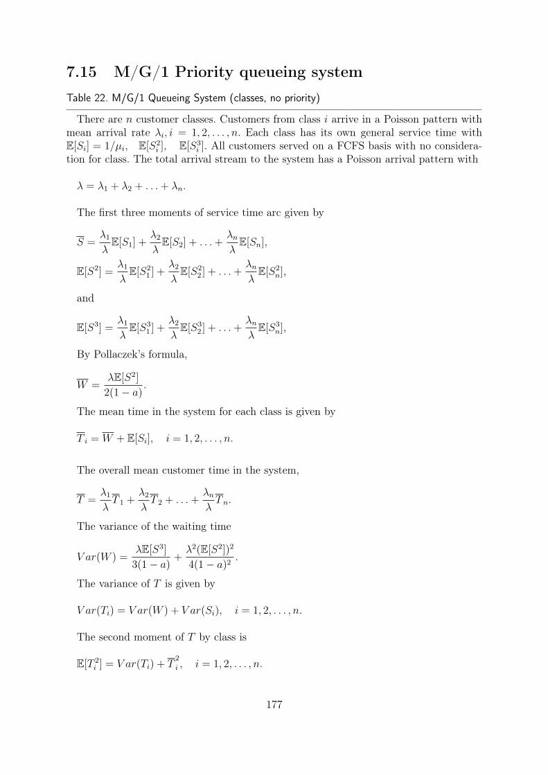
7.15 M/G/1 Priority queueing systemTable 22. M/G/1 Queueing System (classes, no priority)
There are n customer classes. Customers from class i arrive in a Poisson pattern withmean arrival rate λi, i = 1, 2, . . . , n. Each class has its own general service time withE[Si] = 1/µi, E[S2
i ], E[S3i ]. All customers served on a FCFS basis with no considera-
tion for class. The total arrival stream to the system has a Poisson arrival pattern with
λ = λ1 + λ2 + . . .+ λn.
The first three moments of service time arc given by
S =λ1
λE[S1] +
λ2
λE[S2] + . . .+
λnλE[Sn],
E[S2] =λ1
λE[S2
1 ] +λ2
λE[S2
2 ] + . . .+λnλE[S2
n],
and
E[S3] =λ1
λE[S3
1 ] +λ2
λE[S3
2 ] + . . .+λnλE[S3
n],
By Pollaczek’s formula,
W =λE[S2]
2(1− a).
The mean time in the system for each class is given by
T i = W + E[Si], i = 1, 2, . . . , n.
The overall mean customer time in the system,
T =λ1
λT 1 +
λ2
λT 2 + . . .+
λnλT n.
The variance of the waiting time
V ar(W ) =λE[S3]
3(1− a)+λ2(E[S2])2
4(1− a)2.
The variance of T is given by
V ar(Ti) = V ar(W ) + V ar(Si), i = 1, 2, . . . , n.
The second moment of T by class is
E[T 2i ] = V ar(Ti) + T
2
i , i = 1, 2, . . . , n.
177

Table 22. M/G/1 Queueing System (classes, no priority)(continued)
Thus, the overall second moment of T is given by
E[T 2] =λ1
λE[T 2
1 ] +λ2
λE[T 2
2 ] + . . .+λnλE[T 2
n ],
and
V ar(T ) = E[T 2]− T 2.
http://irh.inf.unideb.hu/user/jsztrik/education/03/EN/MG1NoPrio/MG1NoPrio.html
178
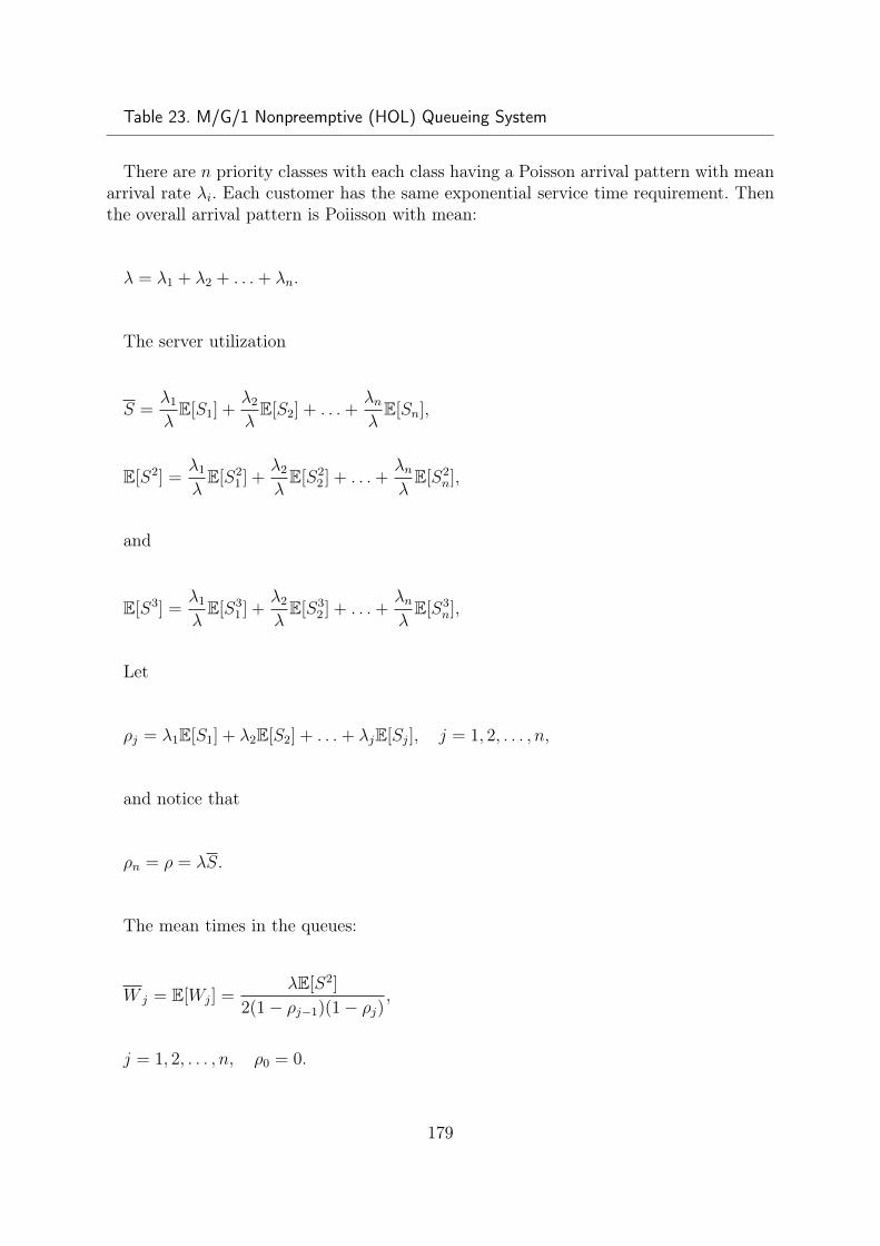
Table 23. M/G/1 Nonpreemptive (HOL) Queueing System
There are n priority classes with each class having a Poisson arrival pattern with meanarrival rate λi. Each customer has the same exponential service time requirement. Thenthe overall arrival pattern is Poiisson with mean:
λ = λ1 + λ2 + . . .+ λn.
The server utilization
S =λ1
λE[S1] +
λ2
λE[S2] + . . .+
λnλE[Sn],
E[S2] =λ1
λE[S2
1 ] +λ2
λE[S2
2 ] + . . .+λnλE[S2
n],
and
E[S3] =λ1
λE[S3
1 ] +λ2
λE[S3
2 ] + . . .+λnλE[S3
n],
Let
ρj = λ1E[S1] + λ2E[S2] + . . .+ λjE[Sj], j = 1, 2, . . . , n,
and notice that
ρn = ρ = λS.
The mean times in the queues:
W j = E[Wj] =λE[S2]
2(1− ρj−1)(1− ρj),
j = 1, 2, . . . , n, ρ0 = 0.
179

Table 23. M/G/1 Nonpreemptive (HOL) Queueing System(continued)
The mean queue lengths are
Qj = λj ·W j, j = 1, 2, . . . , n.
The unified time in the queue
W =λ1
λE[W1] +
λ2
λE[W2] + . . .+
λnλE[Wn].
The mean times of staying in the system
T j = E[Tj] = E[Wj] + E[Sj], j = 1, 2, . . . , n,
and the average of the customers staying at the system is
N j = λj · T j, j = 1, 2, . . . , n.
The total time in the system
T = W + S.
The total queue length
Q = λ ·W ,
and the average of the customers staying at the system
N = λ · T .
The variance of the total time stayed in the system by class
V ar(Tj) = V ar(Sj) +λE[S3]
3(1− ρj−1)2(1− ρj)
+
λE[S2]
(2
j∑i=1
λiE[S2i ]− λE[S2]
)4(1− ρj−1)2(1− ρj)2
+
λE[S2]j−1∑i=1
λiE[S2i ]
2(1− ρj−1)3(1− ρj), j = 1, 2, . . . , n.
180
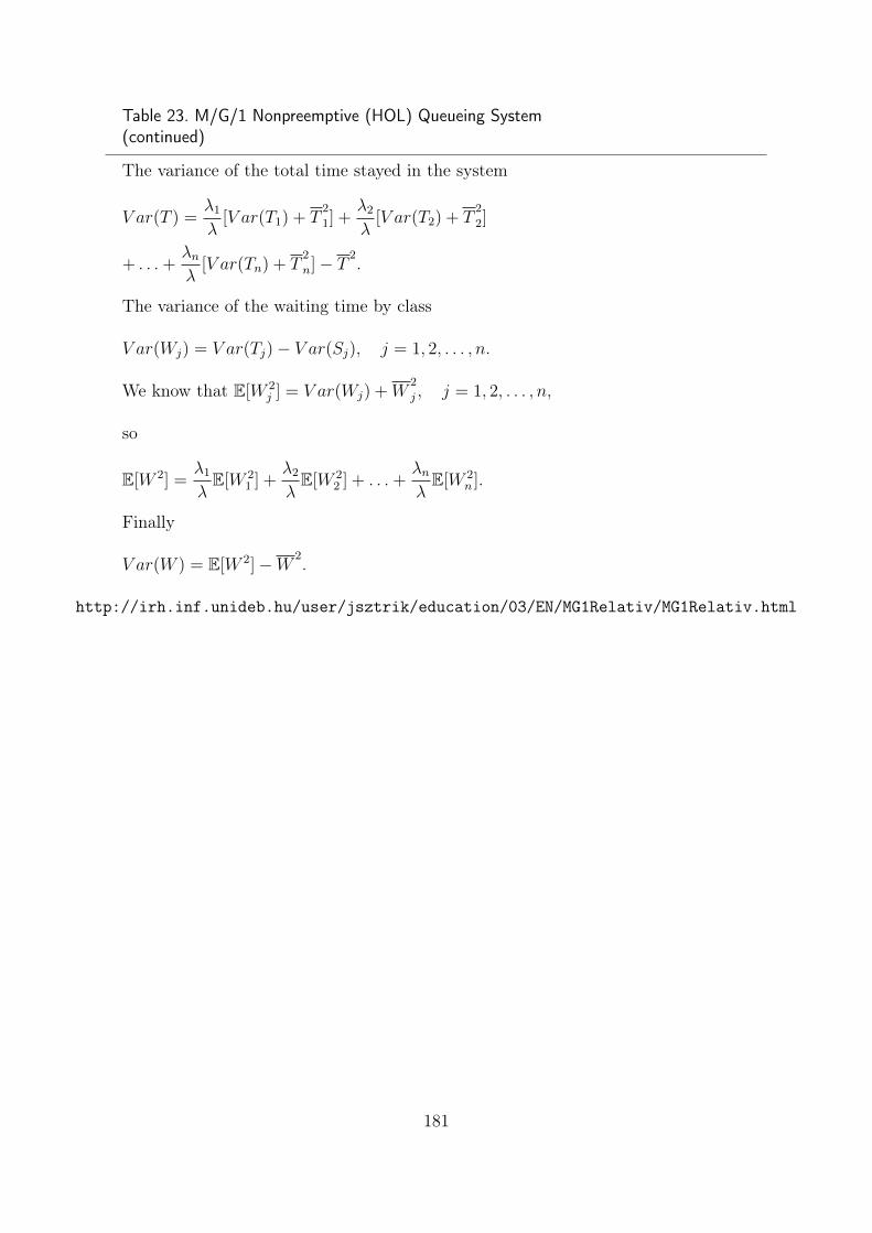
Table 23. M/G/1 Nonpreemptive (HOL) Queueing System(continued)
The variance of the total time stayed in the system
V ar(T ) =λ1
λ[V ar(T1) + T
2
1] +λ2
λ[V ar(T2) + T
2
2]
+ . . .+λnλ
[V ar(Tn) + T2
n]− T 2.
The variance of the waiting time by class
V ar(Wj) = V ar(Tj)− V ar(Sj), j = 1, 2, . . . , n.
We know that E[W 2j ] = V ar(Wj) +W
2
j , j = 1, 2, . . . , n,
so
E[W 2] =λ1
λE[W 2
1 ] +λ2
λE[W 2
2 ] + . . .+λnλE[W 2
n ].
Finally
V ar(W ) = E[W 2]−W 2.
http://irh.inf.unideb.hu/user/jsztrik/education/03/EN/MG1Relativ/MG1Relativ.html
181

Table 24. M/G/1 absolute priority Queueing System
There are n customer classes. Class 1 customers receive the most favorable treatment;class n customers receive the least favorable treatment. Customers from class i arrive ina Poisson pattern with mean arrival rate λi,t = 1, 2, . . . , n. Each class has its own gen-eral service time with E[Si] = 1/µi, and finite second and third moments E[S2
i ], E[S3i ].
The priority system is preemptive resume, which means that if a customer of class j isreceiving service when a customer of class i < j arrives, the arriving customer preemptsthe server and the customer who was preempted returns to the head of the line for classj customers. The preempted customer resumes service at the point of interruption uponreentering the service facility. The total arrival stream to the system has a Poisson arrivalpattern with
λ = λ1 + λ2 + . . .+ λn.
The first three moment of service time are given by:
S =λ1
λE[S1] +
λ2
λE[S2] + . . .+
λnλE[Sn],
E[S2] =λ1
λE[S2
1 ] +λ2
λE[S2
2 ] + . . .+λnλE[S2
n],
E[S3] =λ1
λE[S3
1 ] +λ2
λE[S3
2 ] + . . .+λnλE[S3
n].
Let
ρj = λ1E[S1] + λ2E[S2] + . . .+ λjE[Sj], j = 1, 2, . . . , n,
and notice that
ρn = ρ = λS.
The mean time in the system for each class is
T j = E[Tj] =1
1− ρj−1
E[Sj] +
j∑i=1
λiE[S2i ]
2(1− ρj)
,ρ0 = 0, j = 1, 2, . . . , n.
182
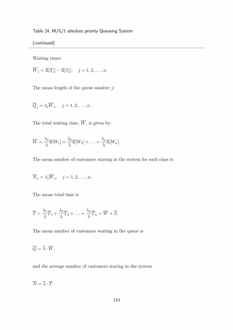
Table 24. M/G/1 absolute priority Queueing System
(continued)
Waiting times
W j = E[Tj]− E[Sj], j = 1, 2, . . . , n.
The mean length of the queue number j:
Qj = λjW j, j = 1, 2, . . . , n.
The total waiting time, W , is given by:
W =λ1
λE[W1] +
λ2
λE[W2] + . . .+
λnλE[Wn].
The mean number of customers staying in the system for each class is
N j = λjW j, j = 1, 2, . . . , n.
The mean total time is
T =λ1
λT 1 +
λ2
λT 2 + . . .+
λnλT n = W + S.
The mean number of customers waiting in the queue is
Q = λ ·W ,
and the average number of customers staying in the system
N = λ · T .
183
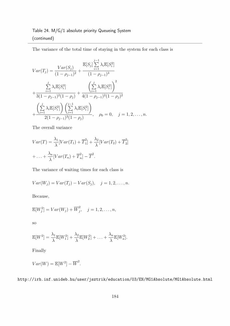
Table 24. M/G/1 absolute priority Queueing System
(continued)
The variance of the total time of staying in the system for each class is
V ar(Tj) =V ar(Sj)
(1− ρj−1)2+
E[Sj]j−1∑i=1
λiE[S2i ]
(1− ρj−1)3
+
j∑i=1
λiE[S3i ]
3(1− ρj−1)2(1− ρj)+
(j∑i=1
λiE[S2i ]
)2
4(1− ρj−1)2(1− ρj)2
+
(j∑i=1
λiE[S2i ]
)(j−1∑i=1
λiE[S2i ]
)2(1− ρj−1)3(1− ρj)
, ρ0 = 0, j = 1, 2, . . . , n.
The overall variance
V ar(T ) =λ1
λ[V ar(T1) + T
2
1] +λ2
λ[V ar(T2) + T
2
2]
+ . . .+λnλ
[V ar(Tn) + T2
n]− T 2.
The variance of waiting times for each class is
V ar(Wj) = V ar(Tj)− V ar(Sj), j = 1, 2, . . . , n.
Because,
E[W 2j ] = V ar(Wj) +W
2
j , j = 1, 2, . . . , n,
so
E[W 2] =λ1
λE[W 2
1 ] +λ2
λE[W 2
2 ] + . . .+λnλE[W 2
n ].
Finally
V ar(W ) = E[W 2]−W 2.
http://irh.inf.unideb.hu/user/jsztrik/education/03/EN/MG1Absolute/MG1Absolute.html
184

7.16 M/G/c Processor Sharing system
Table 25. M/G/1 processor sharing Queueing SystemThe Poisson arrival stream has an average arrival rate of λ and the average service
rate is µ. The service time distribution is general with the restriction that its Laplacetransform is rational, with the denominator having degree at least one higher than thenumerator. Equivalently. the service time, s, is Coxian. The priority system is processor-sharing, which means that if a customer arrives when there are already n− 1 customersin the system, the arriving customer (and all the others) receive service at the averagerate µ/n. Then Pn = ρn(1− ρ), n = 0, 1, . . . , where ρ = λ/µ. We also have
N =ρ
1− ρ, E[T |S = t] =
t
1− ρ, and T =
S
1− ρ.
Finally
E[W |S = t] =ρt
1− ρ, and W =
ρS
1− ρ.
http://irh.inf.unideb.hu/user/jsztrik/education/03/EN/MG1Process/MG1Process.html
Table 26. M/G/c processor sharing Queueing System
The Poisson arrival stream has an average arrival rate of λ. The service time distributionis general with the restriction that its Laplace transform is rational, with the denominatorhaving degree at least one higher than the numerator. Equivalently, the service time, s,is Coxian. The priority system is processor-sharing, which works as follows. When thenumber of customers in the service center, is less than c, then each customers is servedsimultaneously by one server; that is, each receives service at the rate µ. When N > c.each customer simultaneously receives service at the rate cµ/N . We find that just as forthe M/G/l processor-sharing system.
185
7.17 M/M/c Priority systemTable 27. M/M/c relative priority (HOL) Queueing System
There are n priority classes with each class having a Poisson arrival pattern with meanarrival rate λi. Each customer has the same exponential service time requirement. Thenthe overall arrival pattern is Poisson with mean λ = λ1+λ2+. . .+λn. The server utilization
a =λS
c=
λ
cµ,
WW1 =C[c, ρ]S
c(1− λ1S/c),
and thes equations are also true:
W j =C[c, ρ]S
c
[1−
(Sj−1∑i=1
λi
)/c
] [1−
(S
j∑i=1
λi
)/c
] , j = 2, . . . , n.
W j = W j + S, j = 1, 2, . . . , n.
Qj = λj ·W j, j = 1, 2, . . . , n.
N j = λj · T j, j = 1, 2, . . . , n.
W =λ1
λ+λ2
λ+ . . .+
λnλ.
Q = λ ·W .
T = W + S.
N = λ · T .
http://irh.inf.unideb.hu/user/jsztrik/education/03/EN/MMcPrio/MMcPrio.html
186
Bibliography
[1] Adan, I., and Resing, J. Queueing Theory.http://web2.uwindsor.ca/math/hlynka/qonline.html.
[2] Allen, A. O. Probability, statistics, and queueing theory with computer scienceapplications, 2nd ed. Academic Press, Inc., Boston, MA, 1990.
[3] Anisimov, V., Zakusilo, O., and Donchenko, V. Elements of queueing theoryand asymptotic analysis of systems. Visha Skola, Kiev, 1987.
[4] Artalejo, J., and Gómez-Corral, A. Retrial queueing systems. Springer,Berlin, 2008.
[5] Asztalos, D. Finite source queueing systems and their applications to computersystems ( in Hungarian ). Alkalmazott Matemaika Lapok (1979), 89–101.
[6] Asztalos, D. Optimal control of finite source priority queues with computersystem applications. Computers & Mathematics with Applications 6 (1980), 425–431.
[7] Begain, K., Bolch, G., and Herold, H. Practical perfromance modeling, Ap-plication of the MOSEL language. Wiley & Sons, New York, 2001.
[8] Bolch, G., Greiner, S., de Meer, H., and Trivedi, K. Queueing networksand Markov chains, 2nd ed. Wiley & Sons, New York, 2006.
[9] Bose, S. An introduction to queueing systems. Kluwer Academic/Plenum Pub-lishers, New York, 2002.
[10] Breuer, L., and Baum, D. An introduction to queueing theory and matrix-analytic methods. Springer, 2005.
[11] Brockmeyer, E., Halstrom, H., and Jensen, A. The life and works of a.k.erlang. Academy of Technical Sciences, Copenhagen (1948).
[12] Bunday, B., and Scraton, R. The G/M/r machine interference model. EuropeanJournal of Operational Research 4 (1980), 399–402.
[13] Chee-Hock, N., and Boon-He, S. Queueing modelling fundamentals, 2nd ed.Wiley & Son, Chichester, 2002.
187
[14] Cohen, J. The multiple phase service network with generalized processor sharing.Acta Informatica 12 (1979), 245–284.
[15] Cooper, R. Introduction to Queueing Theory, 3-rd Edition. CEE Press, Wash-ington, 1990.http://web2.uwindsor.ca/math/hlynka/qonline.html.
[16] Csige, L., and Tomkó, J. Machine interference problem with exponential dis-tributions ( in Hungarian ). Alkalmazott Matematikai Lapok (1982), 107–124.
[17] Daigle, J. Queueing theory with applications to packet telecommunication.Springer, New York, 2005.
[18] Daigle, J. N. Queueing theory for telecommunications. Addison-Wesley, Reading,MA, 1992.
[19] Dattatreya, G. Performance analysis of queuing and computer networks. CRCPress, Boca Raton, 2008.
[20] Dshalalow, J. H. Frontiers in queueing : Models and applications in science andengineering. CRC Press., Boca Raton, 1997.
[21] Erlang, A. The theory of probabilities and telephone conversations. Nyt Tidsskriftfor Matematik B 20 (1909), 33–39.
[22] Erlang, A. Solution of some problems in the theory of probabilities of significancein automatic telephone exchanges. The Post Office Electrical Engineers’ Journal10 (1918), 189–197.
[23] Falin, G., and Templeton, J. Retrial queues. Chapman and Hall, London,1997.
[24] Fazekas, I. Theory of probability ( in Hungarian ). Kossuth Egyetemi Kiadó,Debrecen, 2000.
[25] Franken, P., Konig, D., and Arndt, U. Schmidt, V. Queues and pointprocesses. Academie Verlag, Berlin, 1981.
[26] Gebali, F. Analysis of computer and communication networks. Springer, NewYork, 2008.
[27] Gelenbe, E., and Mitrani, I. Analysis and synthesis of computer systems.Academic Press, London, 1980.
[28] Gelenbe, E., and Pujolle, G. Introduction to queueing networks. Wiley &Sons, Chichester, 1987.
[29] Gnedenko, B., Belyayev, J., and Solovyev, A. Mathematical methods ofreliability theory ( in Hungarian ). Műszaki Könyvkiadó, Budapest, 1970.
[30] Gnedenko, B., Belyayev, Y., and Solovyev, A. Mathematical methods ofreliability theory. Academic Press, New York, London, 1969.
188
[31] Gnedenko, B., and Kovalenko, I. Introduction to queueing theory.Birkhaeuser, Boston, MA, 1991.
[32] Gross, D., Shortle, J., Thompson, J., and Harris, C. Fundamentals ofqueueing theory, 4th edition. John Wiley & Sons, New York, 2008.
[33] Györfi, L., and Páli, I. Queueing theory in informatics systems (in Hungarian).Műegyetemi Kiadó, Budapest, 1996.
[34] Haghighi, A., and Mishev, D. Queueing models in industry and business. NovaScience Publishers, Inc., New York, 2008.
[35] Hall, R. W. Queueing methods for services and manufacturing. Prentice Hall,Englewood Cliffs, NJ, 1991.
[36] Haribaskaran, G. Probability, queueing theory and reliability engineering. LaxmiPublications, Bangalore, 2006.
[37] Haverkort, B. Performance of computer communication systems: A model-basedapproach. Wiley & Sons, New York, 1998.
[38] Hlynka, M. Queueing Theory Page.http://web2.uwindsor.ca/math/hlynka/queue.html.
[39] Ivcsenko, G., Kastanov, V., and Kovalenko, I. Theory of queueing systems.Nauka, Moscow, 1982.
[40] Iversen, V. Teletraffic Engineering Handbook. ITC in Cooperation with ITU-DSG2, 2005.http://web2.uwindsor.ca/math/hlynka/qonline.html .
[41] Jain, R. The art of computer systems performance analysis. Wiley & Sons, NewYork, 1991.
[42] Jaiswal, N. Priority queues. Academic Press, New York, 1969.
[43] Jereb, L., and Telek, M. Queueing systems ( in Hungarian ). teaching material,BME Department of Telecommunication.http://webspn.hit.bme.hu/˜telek/notes/sokfelh.pdf.
[44] Karlin, S., and Taylor, H. Stochastic process ( in Hungarian ). GondolatKiadó, Budapest, 1985.
[45] Karlin, S., and Taylor, H. An introduction to stochastic modeling. Harcourt,New York, 1998.
[46] Khintchine, A. Mathematical methods in the theory of queueing. Hafner, NewYork, 1969.
[47] Kleinrock, L. Queueing systems. Vol. I. Theory. John Wiley & Sons, New York,1975.
189

[48] Kleinrock, L. Queueing systems. Vol. I. Theory ( in Hungarian ). MűszakiKiadó, Budapest, 1975.
[49] Kleinrock, L. Queueing systems. Vol. II: Computer applications. John Wiley &Sons, New York, 1976.
[50] Kobayashi, H. Modeling and Analysis: An Introduction to System PerformanceEvaluation Methodology. Addison-Wesley, Reading, MA, 1978.
[51] Kobayashi, H., and Mark, B. System modeling and analysis: Foundations ofsystem performance evaluation. Pearson Education Inc., Upper Sadle River, 2008.
[52] Korolyuk, V., and Korolyuk, V. Stochastic models of systems. Kluwer Aca-demic Publishers, Dordrecht, London, 1999.
[53] Kovalenko, I., Pegg, P., and Kuznetzov, N. Mathematical theory of reliabil-ity of time dependent systems with practical applications. Wiley & Sons, New York,1997.
[54] Kulkarni, V. Modeling, analysis, design, and control of stochastic systems.Springer, New York, 1999.
[55] Lakatos, L., Szeidl, L., and Telek, M. Algorithms in informatics, Vol. II(in Hungarian). ELTE Eötvös Kiadó, 2005, ch. Queueing theory ( in Hungarian ),pp. 1298–1347.
[56] Lavenberg, S., e. Computer performance modeling handbook. Academic Press,New York, 1983.
[57] Lefebvre, M. Basic probability theory with applications. Springer, 2009.
[58] Mieghem, P. Performance analysis of communications networks and systems.Cambridge University Press, Cambridge, 2006.
[59] Nelson, R. Probability, stochastic processes, and queueing theory, The mathemat-ics of computer performance modeling. Springer-Verlag, New York, 1995.
[60] Ovcharov, L., and Wentzel, E. Applied Problems in Probability Theory. MirPublishers, Moscow, 1986.
[61] Prékopa, A. Probability theory ( in Hungarian ). Műszaki Könyvkiadó, Budapest,1962.
[62] Pósafalvi, A., and Sztrik, J. On the heterogeneous machine interference withlimited server’s availability. European Journal of Operational Research 28 (1987),321–328.
[63] Pósafalvi, A., and Sztrik, J. A numerical approach to the repairman problemwith two different types of machines. Journal of Operational Reseach Society 40(1989), 797–803.
190
[64] Ravichandran, N. Stochastic Methods in Reliability Theory. John Wiley andSons, 1990.
[65] Reimann, J. Probability theory and statistics for engineers ( in Hungarian) .Tankönyvkiadó, Budapest, 1992.
[66] Rényi, A. Probability theory ( in Hungarian ). Tankönyvkiadó, Budapest, 1973.
[67] Ross, S. M. Introduction to Probability Models. Academic Press, Boston, 1989.
[68] Saaty, T. Elements of queueing theory with applications. Dover Publications, Inc.,New York, 1961.
[69] Saaty, T. Elements of Queueing Theory with Applications. McGraw-Hill, 1961.
[70] Sahner, R., Trivedi, K., and Puliafito, A. Performance and reliability anal-ysis of computer systems – An example-based approach using the SHARPE softwarepackage. Kluwer Academic Publisher, Boston, M.A., 1996.
[71] Sauer, C., and Chandy, K. Computer systems performance modelling. PrenticeHall, Englewood Cliffs, N.J., 1981.
[72] Schatte, P. On the finite population G]/M/l queue and its application to mul-tiprogrammed computers. Journal of lnformation Processing and Cybernetics 16(1980), 433–441.
[73] Stewart, W. Introduction to the numerical solution of Markov chains. PrincetonUniversity Press, Princeton, 1995.
[74] Stewart, W. Probability, Markov chains, queues, and simulation. PrincetonUniversity Press, Princeton, 2009.
[75] Stidham, S. Optimal design of queueing systems. CRC Press/Taylor & Francis,2009.
[76] Syski, R. Introduction to Congestion Theory in Telephone Systems, 2nd Edition.North Holland, 2005.
[77] Sztrik, J. On the finite-source ~G/m/r queues. European Journal of OperationalResearch 20 (1985), 261–268.
[78] Sztrik, J. On the n/G/M/1 queue and Erlang’s loss formulas. Serdica 12 (1986),321–331.
[79] Sztrik, J. On the ~G/M/r/FIFO machine interference model with state-dependent speeds. Journal of Operational Researc Society 39 (1988), 201–201.
[80] Sztrik, J. Some contribution to the machine interference problem with hetero-geneous machines. Journal of Information Processing and Cybernetics 24 (1988),137–143.
191
[81] Sztrik, J. An introduction to queueing theory and its applications (in Hungarian).Kossuth Egyetemi Kiadó, Debrecen, 2000.http://irh.inf.unideb.hu/user/jsztrik/education/eNotes.htm.
[82] Sztrik, J. A key to queueing theory with applications (in Hungarian). KossuthEgyetemi Kiadó, Debrecen, 2004.http://irh.inf.unideb.hu/user/jsztrik/education/eNotes.htm.
[83] Sztrik, J. Practical queueing theory. Teaching material, Debrecen UniversityEgyetem,Faculty if Informatics, 2005.http://irh.inf.unideb.hu/user/jsztrik/education/09/index.html.
[84] Sztrik, J. Performance modeling of informatics systems ( in Hungarian ). EKFLíceum Kiadó, Eger, 2007.
[85] Takagi, H. Queueing analysis. A foundation of performance evaluation. Volume1: Vacation and priority systems, part 1. North-Holland, Amsterdam, 1991.
[86] Takagi, H. Queueing analysis. A foundation of performance evaluation. Volume2: Finite Systems. North-Holland, Amsterdam, 1993.
[87] Takagi, H. Queueing analysis. A foundation of performance evaluation. Volume3: Discrete-Time Systems. North-Holland, Amsterdam, 1993.
[88] Takács, L. Introduction to the theory of queues. Oxford University Press, NewYork, 1962.
[89] Takács, L. Combinatorial Methods in the Theory of Stochastic Processes. JohnWiley & Sons, 1977.
[90] Tijms, H. Stochastic Modelling and Analysis: A Computational Approach. Wiley& Sons, New York, 1986.
[91] Tijms, H. A first course in stochastic models. Wiley & Son, Chichester, 2003.
[92] Tomkó, J. On sojourn times for semi-Markov processes. Proceeding of the 14thEuropean Meeting of Statisticians, Wroclaw (1981).
[93] Tomkó, J. Sojourn time problems for Markov chains ( in Hungarian ). AlkalmazottMatematikai Lapok (1982), 91–106.
[94] Trivedi, K. Probability and Statistics with Reliability, Queuing, and ComputerScience Applications, 2-nd edition. Wiley & Son, New York, 2002.
[95] Ushakov, I. A., and Harrison, R. A. Handbook of reliability engineering.Transl. from the Russian. Updated ed. John Wiley & Sons, New York, NY, 1994.
[96] van Hoorn, M. Algorithms and approximations for queueing systems. Centrumvoor Wiskunde en Informatica, Amsterdam, 1984.
[97] Virtamo, J. Queueing Theory.http://www.netlab.tkk.fi/opetus/s383143/kalvot/english.shtml .
192

[98] Wentzel, E., and Ovcharov, L. Applied problems in probabbility theory. MirPublisher, Moscow, 1986.
[99] White, J. Analysis of queueing systems. Academic Press, New York, 1975.
[100] Wolf, R. Stochastic Modeling and the Theory of Queues. Prentice-Hall, 1989.
[101] Yashkov, S. Processor-sharing queues: some progress in analysis. Queueing Sys-tems: Theory and Applications 2 (1987), 1–17.
193
Related Documents