Basic mathematical tools A.1 Complex variable analysis notes/files... · Basic mathematical tools ... and may wish to read up on more details in the appropriate mathematical physics

Basic mathematical tools

The following pages provide a brief summary of the mathematical material used in the lectures of 442. No rigorous proofs are provided. The reader unfamiliar with the material will find a distillation of the "bare-bones" facts, and may wish to read up on more details in the appropriate mathematical physics or mathematics textbook, such as Butkov, Applied Mathematics.

A.1 Complex variable analysis

1.1 Complex numbers

The Schrödinger equation is a complex-valued differential equation, and its solutions are complex functions. This behavior of the wavefunction is very important as the basis of quantum mechanical interference effects, and a solid understanding of complex variable analysis is necessary to really appreciate the properties of wavefunctions.

We start with the usual definition i2 1, in terms of which a general complex number can be written as z x iy . For a product of two complex numbers the standard rules of algebra then yield

x iy c id xc yd i xd yc A-1

R

iy

x

I

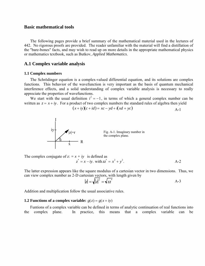
|z|=r Fig. A-1. Imaginary number in the complex plane.

The complex conjugate of z: = x + iy is defined asz* x iy. with zz* x2 y2. A-2

The latter expression appears like the square modulus of a cartesian vector in two dimensions. Thus, we can view complex number as 2-D cartesian vectors, with length given by

z z2 zz* A-3

Addition and multiplication follow the usual associative rules.

1.2 Functions of a complex variable: g(z) g(x iy)

Funtions of a complex variable can be defined in terms of analytic continuation of real functions into the complex plane. In practice, this means that a complex variable can be

substituted into standard expressions instead of a real variable, and manipulated using the algebra outlined in a). For example, the exponential funtion becomes

ez exiy exeiy;

eiy 1 iy 1

2y2

i

3!y3...

1 1

2y2

. ..i y

1

3!y3. ..

A-4

The Taylor expansion in the last line corresponds to exp[iy] = cos[y] + i sin[y], the famous Euler formula for the exponentiation of an imaginary number. Note that the square modulus of exp[iy] is always 1, and y can be interpreted as an angular phase factor as it varies from 0 to 2. Any complex number can be written in this exponential form:

x iy rei r x2 y2 tan 1 y

x. A-5

In a similar way, any function of complex variables can be expressed in terms of function of real variables. For example,

ln z ln x iy ln re i ln r ln e i lnr i , A-6

so the natural logarithm of a complex number automatically yields r and separated in its real and imaginary parts. Since the cos[] and sin[] funtion in the Euler formula cycle after 2 , it is clear that some complex funtions will be multivalued, just as the real square-root function is twovalued. Consider the square root function

f z z1

2 re i 1

2 r1

2 ei2 A-7

This function does not return to its original value after we traverse a circle in the complex plane and return to the x axis:

0 to 2 , f r12 to r

12

2 to 4 , f r1

2 to r1

2

two different functions. A-8

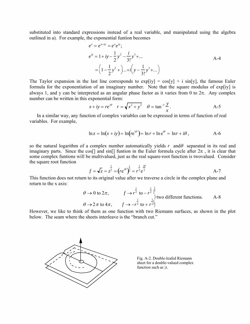
However, we like to think of them as one function with two Riemann surfaces, as shown in the plot below. The seam where the sheets interleave is the “branch cut.”

Fig. A-2. Double-leafed Riemann sheet for a double-valued complex function such as ¦z.

1.3 Derivatives of complex functions

Let f z F x iy u x, y iv x, y ; what is f

z?

Calculus of complex functions is built along the same lines as real calculus; however, derivatives can now be taken in many directions in the complex plane, as opposed to along a single variable axis. This introduces additional constraints on complex functions in order to satisfy continuity. As usual,

fz

fz

F x x i y y F x iy

x iy

u x x, y y u x,y i v x x,y y v x, y

x iy

A-9

This derivative should be uniquely defined in terms of z, no matter what the direction of approach. For simplicity, consider derivatives taken along the real (x) and imaginary (y) axes:

Let y 0 appr. to real axis fz

ux

ivx

Let x 0 appr. to imag axis fz

iuy

vy

u

xv

y&

v

x

u

y

A-10

Continuity (identity) of the derivatives can only be satisfied simultaneously if the real and imaginary parts of the derivatives can be identified, resulting in the Cauchy-Riemann relations to the right. Therefore, not just any combination of x's, y's and i's is a proper complex function of the variable z = x + iy , e.g. f = x2 + i y is not a complex function. To verify the Cauchy-Riemann equations, consider for example the ln[] function:

f z ln z f z 1z 1

x iy x iy

x2 y2

u x

x2 y2 ,u

x

1

x2 y2 2x2

x2 y2 2

y2 x2

x2 y2 2

v y

x2 y2,

v

y

1

x2 y2

2y2

x2 y2 2

y2 x 2

x2 y2 2

A-11

and similarly for the other Cauchy-Riemann relation. To summarize: generally we can take derivatives as for any real function, but NOT ANY u x, y iv x, y is a legal complex function.

1.4 Complex integrals

Integrals in the complex plane follow a contour line C( x=x(t), y=y(t) ), much like line integrals in the x-y plane. However, since f(z) cannot be a completely arbitrary function of the real and imaginary parts of z, contour integrals have certain special properties. We can write any contour integral as two line integrals over vector functions F and G to separate real and imaginary parts:

f z dzC u iv dx idy

C

udx vdy C i vdx udy

C F dx

C i G dx

C

A-12

where F u x,y ˆ x v x, y ˆ y and G u x, y ˆ x v x, y ˆ y . Finally, if we choose a specific curve C with x = x(t) and y = y(t), the line integrals become

f z dzC u

dxdt

dt v

dydt

C (t ) i . ..

C ,

F dx

dt

dt

C i G

dx

dt

dt

C

. A-13

z

f(z)

x

y

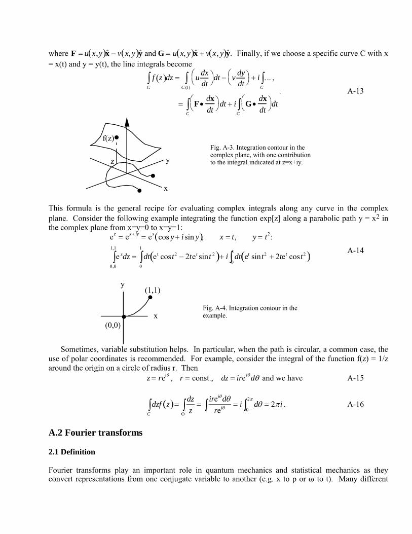
Fig. A-3. Integration contour in the complex plane, with one contribution to the integral indicated at z=x+iy.

This formula is the general recipe for evaluating complex integrals along any curve in the complex plane. Consider the following example integrating the function exp[z] along a parabolic path y = x2 in the complex plane from x=y=0 to x=y=1:

ez ex iy ex cos y i sin y , x t, y t2:

e zdz0,0

1,1

dt et cos t2 2te t sint 2 0

1

i dt et sint2 2te t cost2 0

1

A-14

x

y(1,1)

(0,0)

Fig. A-4. Integration contour in the example.

Sometimes, variable substitution helps. In particular, when the path is circular, a common case, the use of polar coordinates is recommended. For example, consider the integral of the function f(z) = 1/z around the origin on a circle of radius r. Then

z rei , r const., dz ire id and we have A-15

dzf z C

dz

z

ireidrei i d 2i

0

2

. A-16

A.2 Fourier transforms

2.1 Definition

Fourier transforms play an important role in quantum mechanics and statistical mechanics as they convert representations from one conjugate variable to another (e.g. x to p or to t). Many different

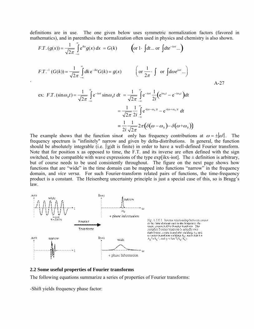
definitions are in use. The one given below uses symmetric normalization factors (favored in mathematics), and in parenthesis the normalization often used in physics and chemistry is also shown.

`

F.T . (g(x)) 1

2eikxg(x) dx

G(k) or 1 dt... or dte i t ...

F.T .1 (G(k)) 1

2dk e ikxG(k

) g(x) or1

2 or dei t ...

ex: F.T . (sin0t) 1

2e i t sin0t dt

1

2e i t 1

2iei0 t e i0 t dt

1

21

2ie-i( 0 )t e-i( 0 )t dt

1

2i

1

22 0 +0

A-27

The example shows that the function sint only has frequency contributions at ' . The frequency spectrum is "infinitely" narrow and given by delta-distributions. In general, the function should be absolutely integrable (i.e. ∫|g|dt is finite) in order to have a well-defined Fourier transform. Note that for position x as opposed to time, the F.T. and its inverse are often defined with the sign switched, to be compatible with wave expressions of the type exp[ikx-it]. The ± definition is arbitrary, but of course needs to be used consistently throughout. The figure on the next page shows how functions that are “wide” in the time domain can be mapped into functions “narrow” in the frequency domain, and vice versa. For such Fourier-transform related pairs of functions, the time-frequency product is a constant. The Heisenberg uncertainty principle is just a special case of this, so is Bragg’s law.

2.2 Some useful properties of Fourier transforms

The following equations summarize a series of properties of Fourier transforms:

-Shift yields frequency phase factor:

F.T . g x x0 1

2e ikxg(x x0 ) dx

1

2e ikx0 e ikx 'g(x ')dx '

e ikx0 G(k) A-28

-F.T. of derivative turns into product factor (useful for solving differential equations, and important in quantum mechanics to relate x and p):

F.T . g x 1

2dx g x e ikx

1

2g x e ikx

ik e ikxg x

dx

ik F g x ; In general F.T . g n x ik n F.T . g x A-29

-F.T. of a convolution is the product of the F.T (here, let’s use the exp[-it] definition of the Fourier transform, usually used for time variables):

g h 1

2d t g t '

f t t F.T . g h 1

2dt e i t

d t g t ' f t t

1

2d t g t '

dt ei t f t t

(let t t t and dt d t )

1

2d t g t '

d t e i ( t t ) f t

1

2dt 'e i t g t

22

dt"e i t f t

2G F

A-30

The convolution function occurs in many applications, for example the increase in observed linewidths due to convolution of the natural lineshape with a "broadening factor" due to laser resolution, molecular motion (Doppler effect), etc. In a laser autocorrelation function, the output intensity is obtained by convolving the input electric fields with respect to one another:

I(t0 ) dtA t A t0 t

I (t0 )dt | A( ) |2 d

A-31

The formula at the bottom is a form the Wiener-Khintchine theorem, a fundamental theorem of statistical mechanics relating the integral of power over time to the power in the frequency domain. These F.T. formulas are practical because of a computer algorithm known as the FFT developed by Cooley and Tukey in the early 1960s, which allows rapid evaluation of Fourier transforms.

A.3 Linear algebra, function spaces, Dirac notation

Quantum mechanics uses complex-valued wavefunctions to describe the evolution of a system, operators that act on these wavefunctions to transform them into other wavefunctions, and expectation values of operators, which correspond to observable quantities. This is directly analogous to vectors, matrices that act on them to yield other vectors, and scalar products of vectors with such transformed vectors:

| v

ˆ A | |' Av v'

| ˆ A | |' v (Av) v v'

A-32

The analogy is twofold: the function space of wavefunctions is directly analogous to the n-dimensional vector spaces of linear algebra; and by using basis set representations of wavefunctions and operators, the quantum mechanical problem in effect becomes a linear algebra problem. We briefly review these issues below.

3.1 Hilbert space

Among the many notations attempted for quantum mechanics, the most powerful has proven to be in terms of a "function space", in which the functions can be thought of as vectors, much like n-dimensional vectors in ordinary vector space. To be useful for quantum mechanics, such a function space h must have a number of properties:

-The functions must have a norm ||. In practice ∫dxk*k = 1 is the square of this norm (∫dxk*k' = (k-k') for free particles).

-There exists a scalar product operation < | > which maps any two functions , 'h onto the complex numbers with properties analogous to ordinary scalar products. In practice, this is done by an operation

dx*(x)_ . The complete set of operations dx*(x)_ for all h also form a space, the dual space h* of h. The recipe for computing the scalar product of and ' is as follows: take the operation

dx*(x)_ dual to , insert ' in the placeholder _. The results is the scalar product <|'>, a complex number. In particular, √<|> is the positive-definite norm of . Also, <'|> = <|'>*.

The first of these properties is sufficient for a "Banach space" h. An entity H = (h; < | >) which consists of a Banach space on which a scalar product is defined, is known as a "Hilbert space". These concepts are entirely analogous to the ones from ordinary linear algebra. For example, an ordinary vector v is element of a vector space V. The norm of v is the length of that vector. The dual space of V has elements v. which are operations acting on the vV, and the scalar product between v and v' is defined as v.v'. The norm is v .

vFor a Hilbert space, we can define a complete orthonormal basis {i}. Orthonormal implies

<i|j>=i,j. Completeness implies that any function H can be expressed as a linear combination of these basis functions. (If not, we would add the part of that's left over as another basis function to obtain completeness!) This implies that can be fully characterized by its scalar products <|i> with the basis functions i. These scalar products can be assembled into a vector c with coefficients <|i> and the same dimension as the Hilbert space. This allows one to reduce function spaces to ordinary vector spaces, as discussed below.

3.2 Dirac notation and operators

Functions such as can be expressed in terms of many different kinds of variables such as x or p, depending on what is most convenient. Very often, one only wants to discuss the functions themselves, irrespective of which variables they are represented in terms of. It is then convenient to use the bracket notation of Dirac and replace

H by the ket |>dx*(x)_ H* by the bra <|. A-33

Note that while |> is indeed the function as an abstract member of the function space H , <| is not *(x) or any function at all, but rather an overlap operation in the dual space h*. Lack of realization of this fact leads to endless confusion and misuse of the Dirac notation.

We now have a compact representation for functions and their overlap integrals (or scalar products) with other functions. The final ingredient is the addition of linear operators, which can turn functions into new functions. Again, the best analogy is conventional vector space: v' = a v where a is a scalar. The new vector v' points in the same direction as v, but has different normalization. Similarly ' = a . To change the orientation of a vector, we need to apply a matrix M: v' = M v. M may induce a translation, rotation, or shearing on the vector. Similarly we can have ' = M., where M is a linear operator (i.e. it acts on to the first power as shown). A wide class of linear operators is allowed, such as differentiation, multiplication by another function, etc. Consider for example the angular-variable function () acted on by operator exp[d/d]:

ed / d() (1 dd 1

2 2 d2

d2 )

( )A-34

Clearly, exp[d/d] is the wavefunction equivalent of a rotation matrix for a vector, rotating the wavefunction by an angle The analogy with linear algebra vector spaces is even more direct. Let us express wavefunctions and ' in terms of their coefficients ci and ci' in a basis {i} as vectors c and c'. Then ci=∫dxi* and ci'=∫dxi*'. We can compute "matrix elements" of any operator M using the dual basis: Mij <i|M|j> . If ' = M., then dxi

* ' dxi* M

dxi* cj

' j dxi* M cj j

cj' i | M| j ci or

c' Mc or

|' M |

The first step simply involves application of the "overlap operator"; in the second step, and ' are expressed in terms of the basis; the third step switches to Dirac notation for the overlap integrals, AND assumes the basis functions are orthonormal. Steps 4 and 5 are the same as step 3, in pure algebra or pure Dirac notation.

Thus, acting with an operator on a wavefunction can be replaced by a linear algebra problem of matrix multiplication if we write the wavefunction as a vector of basis set coefficients, and the operator as a matrix of overlap integrals. Dirac notation is an intermediate form of notation which allows us to write equations in terms of the abstract wavefunction, its "dual" bra, and abstract operators without reference to a basis, while maintaining the simplicity of pure matrix notation.

In the above, the dual space overlap operation dx*(x)_ is referred to as an operation, not an operator. This is because its application to a wavefunction yields a scalar (the overlap coefficient ci) rather than another function, as an operator would. We can write an operator which is the direct analog of the dual space operators as follows:

Pi i dx i* _|i i |

When applied to a function , Pi computes its overlap with i and returns the function i times that overlap. It effectively projects the part of that looks like i out and returns it. Hence Pi is referred to as a projection operator. Generally, operators can be constructed by combining functions h and duals h* in "reverse" order from matrix elements.3.3 Hermitian operators

Since observable quantities must be real (as far as we know) and are interpreted as expectation values in quantum mechanics, operators with real expectation values are of particular interest. For a matrix to have this property, it must be Hermitian, i.e. it must equal its complex conjugate-transpose: M = M†. An analogous property must therefore hold for Hermitiean operators. For any operator,

F F F F† A-37

The fourth step can be taken as the definition of the hermitian conjugate F† of F. In the special case of hermitian operators F F

must hold for any matrix elements in any basis representation, or the expectation values will not be real. This immediately implies that F = F† must hold for a hermitian operator, i.e. in its matrix representation it must equal its own complex conjugate-transpose. This can easily be shown in matrix notation:

Let F ciFijdj

i , j

or

c1* c2

* di

* i

i

f11 f12

f21 f 22

d1

d2

di ii

c1 f11d1 c1

* f12d2 A-38

We claim that the complex conjugate transpose matrix element of operator f†, namely

d1 d2

f11 f12

f 21 f22

c1

c2

d1 f11

c1 d1 f12 c2 d2 f 21

c1

F 21

* f12 or F

12 f12

A-39

should be the same. As shown by the one example of f12 by comparison of the two explicit equations, this is indeed the case, if we make use of the hermitian property of the operator's matrix representation.

3.4 Other useful matrix properties

-Inverse, transpose, and complex-conjugate transpose of products:

AB 1 B1A1

AB Š %B %A

A-40

These can be shown by direct evaluation:

a11 a12

a21 a22

b11 b12

b21 b22

a11b12 a12b22

a21b11 a22b21

a21

* b11* a22

* b21*

a11* b12

* a12* b22

* ...

-Antihermitian property of commutators:Let A and B be hermitian; thenA,B AB BA BA AB BA AB A,B A-41

This implies that [A,B] is anti-Hermitian: its Hermitian conjugate equals minusitself. [A,B] can therefore be written as iC, where C is a Hermitian operator.

-Diagonalization of Hermitian matrices by unitary matrices:Let M1HM , H is hermitian

M1HM MH M1 or M1 M

MM I

A-42

The last property defines M to be a unitary matrix.

3.5 Behavior of the determinant of matrices

i) the determinant of A is the sum over all possible products of matrix elements including only one from each row and column, with a sign alternation for odd and even permutations:

a11 a12 a13

a21 a22 a23

a31 a32 a33

a11

a22 a23

a32 a33

a12

a21 a23

a31 a33

a31 A-43

ex:

deta11 a12

a21 a22

a11a22 a12a21 A-44

Note: det(A) unchanged if we add rows to one another or exchange them.

ii) det AB det A det B A-45

iii) det A1 1

det A since det AA1 det I 1 det A det A1 A-46

iv) a similarity transformation leaves the determinant unchanged:det M1GM det M1 det G det M det G A-47

v) the determinamt of a matrix is just the product of its eigenvalues, since diagonalization is just a similarity transformation:

det G ii

vi) For any matrix, det( ˜ M ) det(M); det(M*) det(M)* A-48

vii) For unitary matrices, det M1 det ˜ M * det M * A-49

det M1M det M1 det M 1 det M det M * 1

or det M e i

Diagonalize

M 1

2

M M1 ii

* 1 or i e ii : A-50

all eigenvalues. of a unitary matrix have unit modulus.

3.6 Matrix diagonalization

Many problems in quantum mechanics can be posed as eigenvalue problems; the most famous is the solution of the time-independent Schrödinger equation for energy eigenvalues. The eigenvalue problem is the following: which functions in H are unchanged by application of a certain operator G, other than a multiplicative factor , referred to as the eigenvalue? If we convert wavefunctions to vectors m, the question becomes: which vectors are unchanged by application of a matrix G, except for a multiplicative factor ?

For hermitian and other well-conditioned matrices, the number of such vectors generally equals the dimension of the vector space. (This is of course infinite for a Hilbert space with infinitely many basis functions.) We can group all these vectors m into a matrix M, and all the eigenvalues into a diagonal matrix , in which case the problem is posed as

GM M or M 1GM A-51awhere the columns of M are the vectors m, and the diagonal elements of are the eigenvalues. Note that the matrix M appears on the LEFT-hand side of . For a single vector m, we can write this explicitly in terms of a set of linear equations to be solved: Gm m , or

(G-I)m = 0; explicitly, A-51b

i 1n: (Gij ij )x j

j1

n

0

It is not generally possible for n sums over n xi variables to be simultaneously zero, unless all xi are identically zero:

ex: z 5x 2 y 0 z 5 x 2 y

2 z 8 x 10 y 0 z 4 x 5y

z 2 x 2 y 0

x 3 y 0 or x 3y , z 17y 17 y 6 y 2 y 0

A-52

However, if one of the equations is redundant (can be expressed in terms of the others), then a solution is possible, where all xi can be determined as multiples of one of them:

ex: z 5x 2y 0

2z 8x 10y 0

4z 18x 14y 0

x 3y, z 17y 6y 54y 14y 0 for any y!

A-53

A condition for such redundancy is that the determinant of the coefficient matrix be zero, or det(G-I) = 0 to make the set of equations singular. The det(G-I) is a polynomial in of order n, where n is the size of the matrix. These eigenvalues can be found by solving the polynomial, and can then be inserted into the linear equations above to yield the components of the eigenvectors.

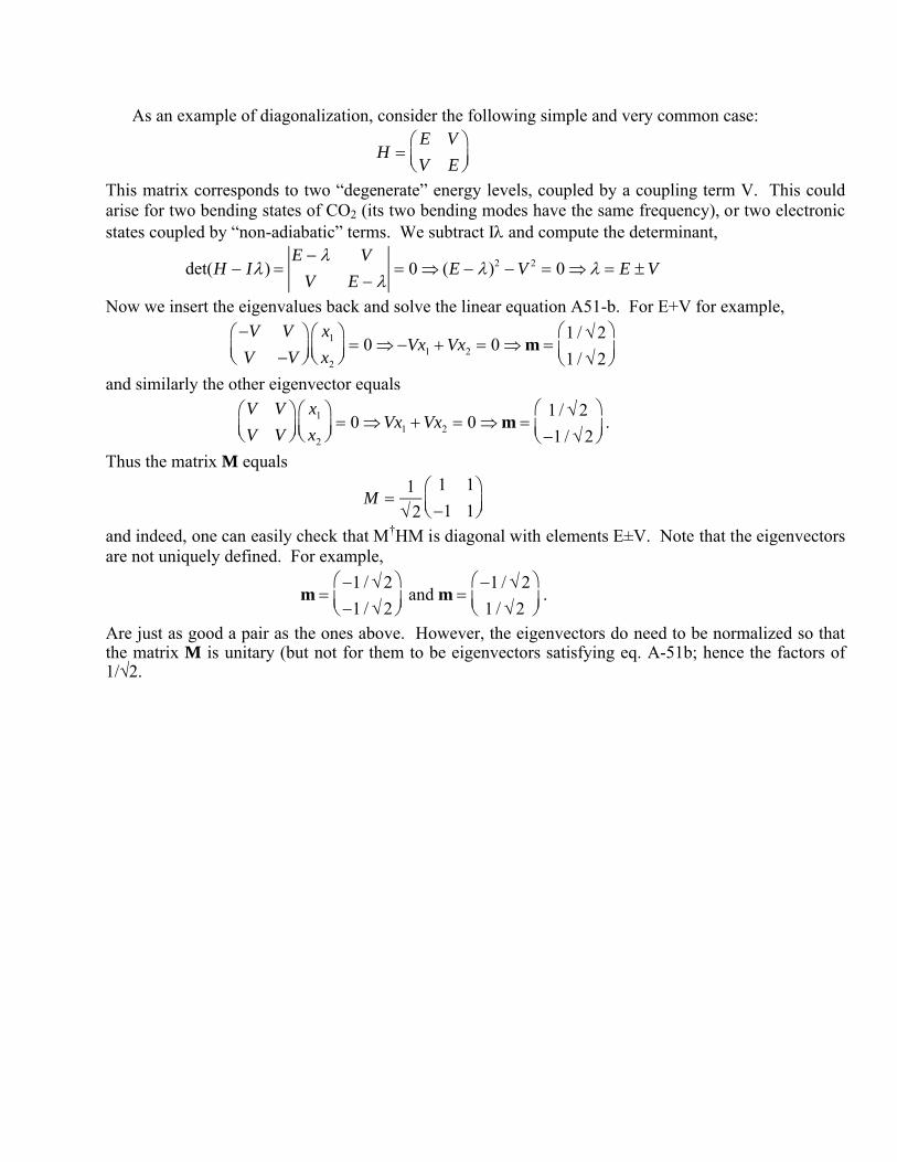
As an example of diagonalization, consider the following simple and very common case:

H E V

V E

This matrix corresponds to two “degenerate” energy levels, coupled by a coupling term V. This could arise for two bending states of CO2 (its two bending modes have the same frequency), or two electronic states coupled by “non-adiabatic” terms. We subtract I and compute the determinant,

det(H I) E V

V E 0 (E )2 V 2 0 E V

Now we insert the eigenvalues back and solve the linear equation A51-b. For E+V for example,

V V

V V

x1

x2

0 Vx1 Vx2 0 m

1 / 2

1 / 2

and similarly the other eigenvector equals

V V

V V

x1

x2

0 Vx1 Vx2 0 m

1 / 2

1 / 2

.

Thus the matrix M equals

M 1

2

1 1

1 1

and indeed, one can easily check that M†HM is diagonal with elements E±V. Note that the eigenvectors are not uniquely defined. For example,

m 1 / 2

1 / 2

and m

1 / 2

1 / 2

.

Are just as good a pair as the ones above. However, the eigenvectors do need to be normalized so that the matrix M is unitary (but not for them to be eigenvectors satisfying eq. A-51b; hence the factors of 1/√2.