Basic Image Processing January 26, 30 and February 1.

Basic Image Processing

January 26, 30 and February 1

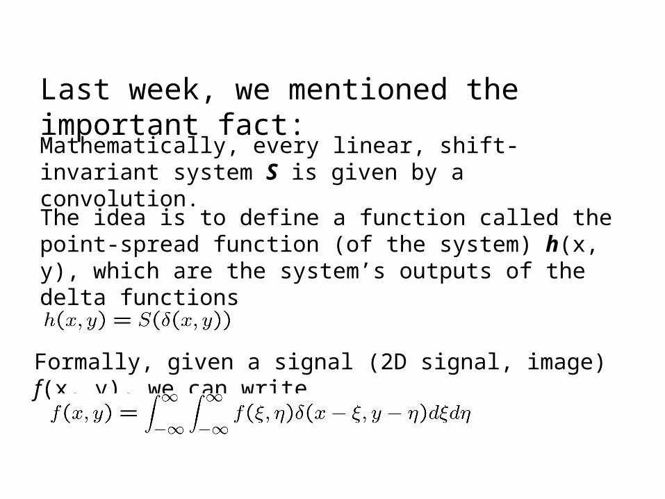
Last week, we mentioned the important fact:

Mathematically, every linear, shift-invariant system S is given by a convolution.

The idea is to define a function called the point-spread function (of the system) h(x, y), which are the system’s outputs of the delta functions

Formally, given a signal (2D signal, image) f(x, y), we can write

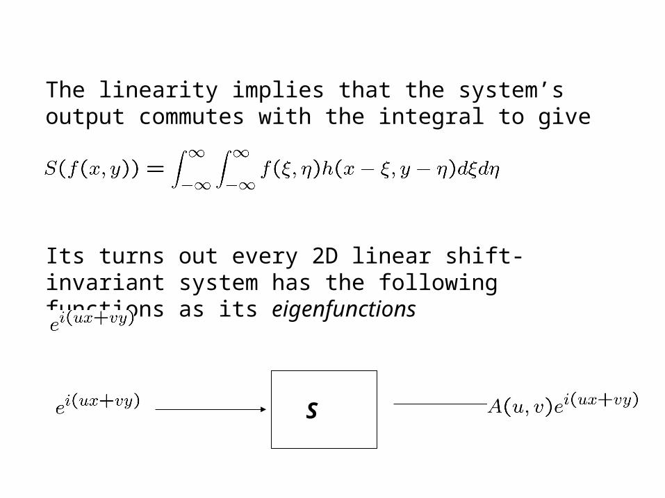
The linearity implies that the system’s output commutes with the integral to give

Its turns out every 2D linear shift-invariant system has the following functions as its eigenfunctions

S

Recall that

The imaginary and real parts can be interpreted as waves

S

H(u, v) is called the modulation-transfer function.

Fourier Transform

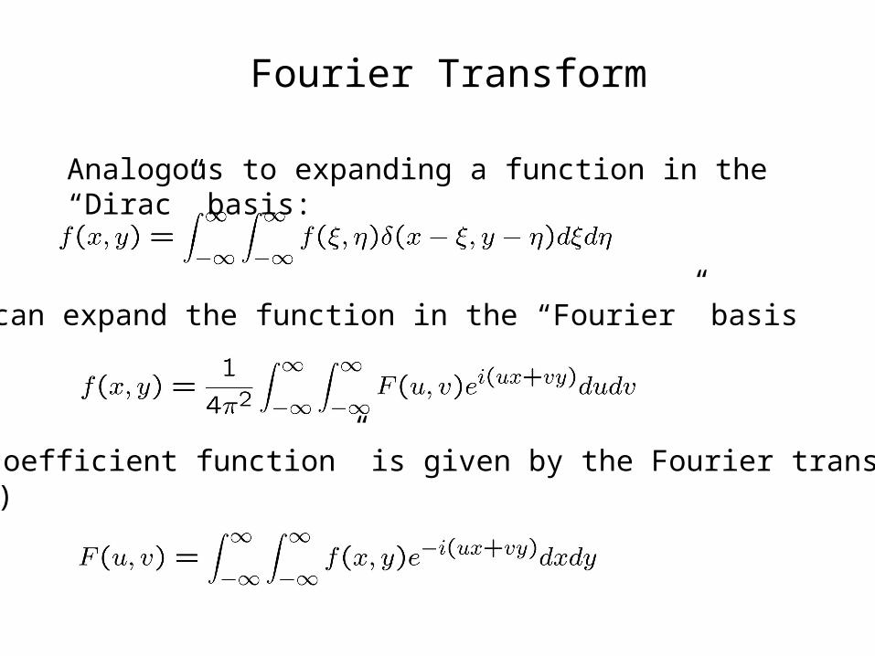
Analogous to expanding a function in the “Dirac” basis:

We can expand the function in the “Fourier” basis

The “coefficient function” is given by the Fourier transform of f(x, y)

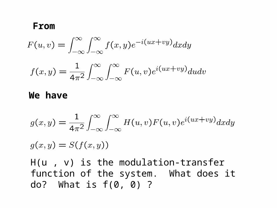
From

We have

H(u , v) is the modulation-transfer function of the system. What does it do? What is f(0, 0) ?

Spatial domain Frequency domain

Domain on which the function is defined

Fourier transform

Inverse Fourier transform

Coefficients of the wave components

Important Properties of Fourier Transform

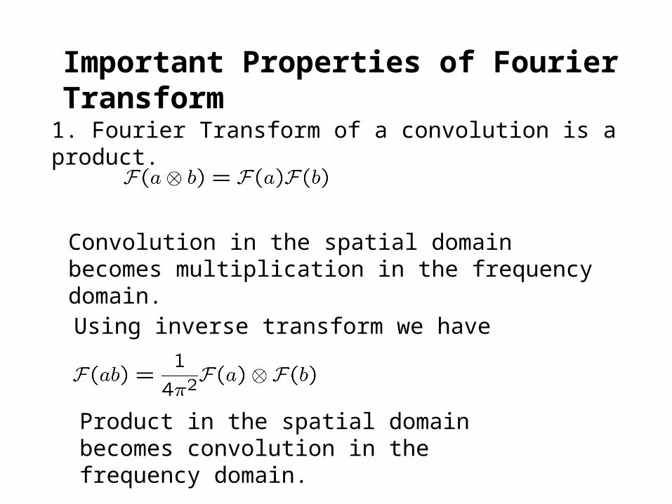
1. Fourier Transform of a convolution is a product.

Convolution in the spatial domain becomes multiplication in the frequency domain.

Using inverse transform we have

Product in the spatial domain becomes convolution in the frequency domain.

Important Properties of Fourier Transform

2. Raleigh’s theorem (Parseval’s theorem)

Important Properties of Fourier Transform

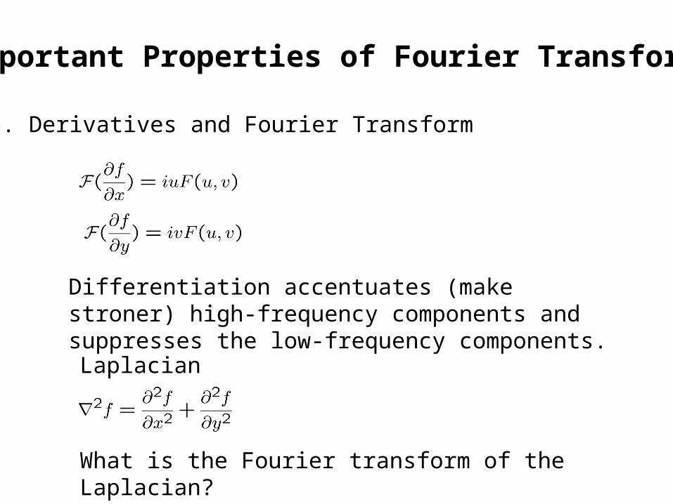
3. Derivatives and Fourier Transform

Differentiation accentuates (make stroner) high-frequency components and suppresses the low-frequency components.

What is the Fourier transform of the Laplacian?

Laplacian

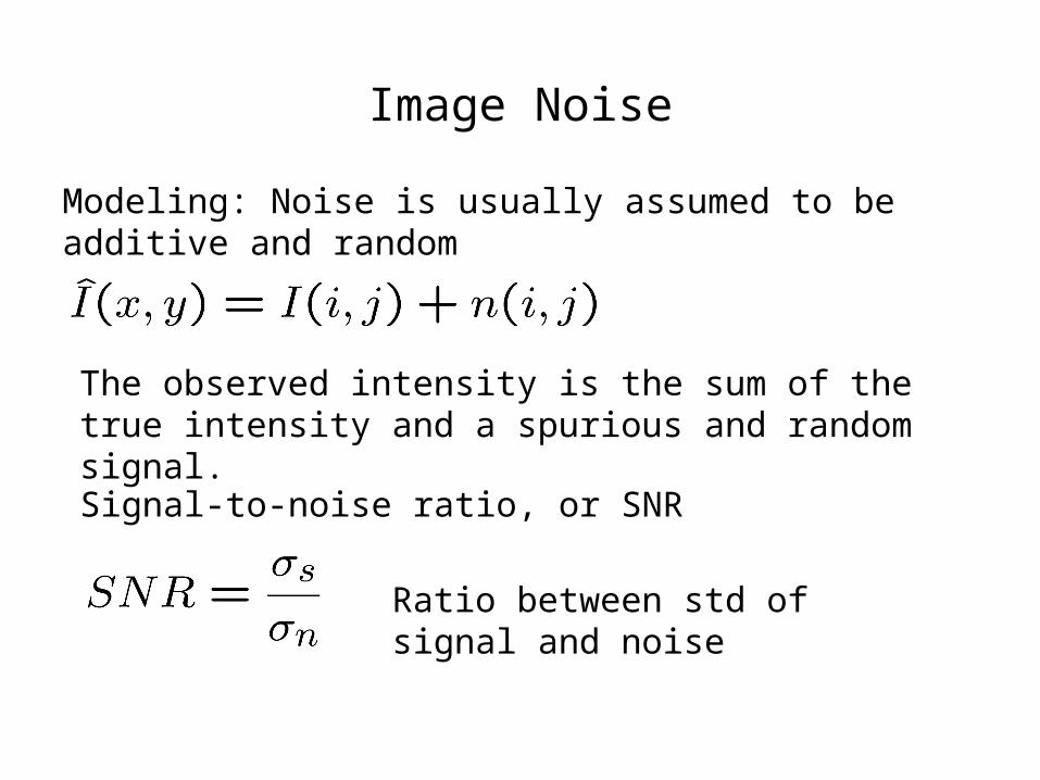
Image Noise

Modeling: Noise is usually assumed to be additive and random

The observed intensity is the sum of the true intensity and a spurious and random signal.

Signal-to-noise ratio, or SNR

Ratio between std of signal and noise

Noise Modeling

In the absence of information, the noise n(i, j) is usually modeled

By a white, Gaussian, zero-mean stochastic proces.

is treated as a random variable, distributed according to a zero mean Gaussian distribution function of fixed standard deviation.

Gaussian distribution

Noise Modeling

Impulsive noise (or peak noise): occur usually in addition to the one normally introduced by acquisition.

x and y are two (uniformly distributed) random variables with range [0, 1].

Original image Salt and pepper noise added

Filtering and Smoothing

Problem: Given an image I corrupted by noise n, attenuate n as much as possible (ideally, eliminate it altogether) without change I significantly.

Linear Filter: Convolving the image with a constant matrix, called mask or kernel.

Mean Filter

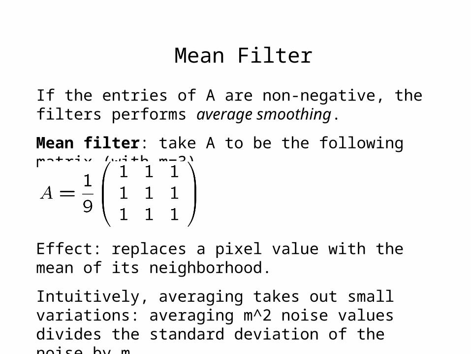
If the entries of A are non-negative, the filters performs average smoothing.

Mean filter: take A to be the following matrix (with m=3)

Effect: replaces a pixel value with the mean of its neighborhood.

Intuitively, averaging takes out small variations: averaging m^2 noise values divides the standard deviation of the noise by m.

The Fourier transform of a 1-D mean filter kernel of with 2W is the sinc function

Signals frequencies falling inside the main lobe are weighted more than the frequencies falling in the secondary lobes, the mean filter can be regarded as an approximate “low-pass”filter.

Gaussian smoothing: Kernel is a 2-D Gaussian.

Fourier transform of a Gaussian is still a Gaussian and no secondary lobes. This makes the Gaussian kernel a better low-pass filter than the mean filter.

Another important fact about Gaussian kernel: It is separable.

Another important fact about Gaussian kernel: It is separable.In practice, this means that the 2D convoluation can be computed first by convolvingg all row and then all columns with a 1-D Gaussian have the same standard deviation.

To be continued …