Basic concepts to understand Gamma Ray Bursts. The waves Direction of propagation perturbation.

basic concepts to understand Gamma Ray

Bursts

The waves

Direction of propagation

perturbation

ELETTROMAGNETIC WAVE

Continuum series of pulses originated from a variation of the electromagnetic field.

It is a perturbation of the electromagnetic field.

The redshift and the distance Measurementredshift:

The light frequency is lower than the frequency was emitted.This happens when the source is receding in the

observer

SUN GALAXY

We look at the spectrum of an electromagnetic light emission of an object and we compare it

with another nearer

EMITTED

OBSERVEDz

1

1EMITTED

OBSERVEDz

Gamma-Ray Bursts: The story Gamma-Ray Bursts: The story beginsbegins

Klebesadel R.W., Strong I.B., Olson R., 1973, Astrophysical Journal, 182, L85

`Observations of Gamma-Ray Bursts of Cosmic Origin’

Brief, intense Brief, intense flashes of flashes of -rays-rays

The Vela are American satellites that try to see if the URSS respects theTreats banning nuclear tests between USA and URSS in the early 60s

They were too much long to be nuclear explosions and too much short to be a known phenomenon!

GRBs phenomenology

Basic phenomenology– Flashes of high energy photons in the sky (typical duration is few seconds).– Isotropic distribution in the sky – Cosmological origin accepted (furthest GRBs observed z ~ 7 – billions of light-years).– Extremely energetic and short: the greatest amount of energy released in a short time (not considering the Big Bang).– Sometimes x-rays and optical radiation observed after days/months (afterglows), distinct from the main γ-ray events

(the prompt emission).– Observed non thermal spectrum

The energetics of GRBs

An individual GRB can release in a matter of seconds the same amount of energy that our Sun will radiate over its 10-billion-year lifetime

Isotropical distribution in the sky

12

Short vs Long GRBs Short vs Long GRBs

Kouveliotou et al., 1996, AIP Conf. Kouveliotou et al., 1996, AIP Conf. Proc., 384, 42.Proc., 384, 42.Paciesas et al., 1999, ApJS, 122, 465.Paciesas et al., 1999, ApJS, 122, 465.Donaghy et al., 2006, Donaghy et al., 2006, astro-ph/0605570.astro-ph/0605570.

Short (hard)Short (hard) Long (soft)Long (soft)

ShortShort GRBs -> TGRBs -> T9090<2 s Long GRBs -> <2 s Long GRBs ->

TT9090>2 s>2 sShort GRBsShort GRBs -> T-> T

9090<5 s Long GRBs<5 s Long GRBs -> ->

TT9090>5 s>5 s Norris et Bonnell 2006

What is the T90

• Time interval in which the instrument reveal the 5% of the total counts and the 90%.

• To the duration of this event it is associated the 90% of the emission

Progenitors for traditional Progenitors for traditional modelmodel core collapse of massive stars (M > 30 Msun)

long GRBs Collapsar or Hypernova (MacFadyen & Woosley 1999 Hjorth et al. 2003; Della Valle et al. 2003, Malesani et al. 2004, Pian et al.

2006) GRB simultaneous with SN

Discriminants: host galaxies, location within host, duration, environment, redshift distribution, ...

compact object mergers (NS-NS, NS-BH) short GRBs

Collapsar model

• Very massive star that collapses in a rapidly spinning BH. • Identification with SN explosion.

Woosley (1993)

prompt emission FRED (Fast Rise, Exponential Decay)

Pre-Swift vs Swift for the afterglows

Typical lightcurve for BeppoSAX Typical lightcurve for Swift

Swift zmedio = 2.5!!!

Pre-Swift zmedio = 1.2

Definition of the Flux and Energy

• The flux F is the energy carried by all rays passing through a given area dA .

• dA normal to the direction of the given ray • all rays passing through dA whose direction is

within a solid angle dΩ of the given ray

• E=Iν *dA*dt*dΩ*dν

• Iv= is the brightness or specific intensity• dFν =E/(dA*dt*dν)

• dF= dIF cos For some arbitrary orientation n

Gamma-ray Burst Real-time Sky Map http://grb.sonoma.edu/

• Burst List• Burst ID GRB 090301A• Date 2009/03/01• Time 06:55:55• Mission Swift• RA 22:32• Dec 26:38• brief Burst Description This burst had a complex multipeak structure and a duration of ~50 seconds. Due to observing constraints Swift cannot slew to this position until after April 15. No XRT or UVOT was available as a result.

SpectraSpectraNon thermal Non thermal spectraspectra

α ~-1β ~ -2 Ebreak ~ 100 keV - MeV

Epeak =(α +2) Ebreak

E

N(E) Eα

Eβ

Ebreak

The phenomenological Band law hold in a wide energy interval 2keV-100MeV

Time [sec]

cts/sec

GRB spectrum evolves with time within GRB spectrum evolves with time within single burstssingle bursts

Hard to soft evolution

featureless continuumfeatureless continuum

power-laws - peak in power-laws - peak in FF F ~ E F ~ E

Epeak

This coefficient α in the L-Ta analysis it isβa (so it will be call the same in the exercise)

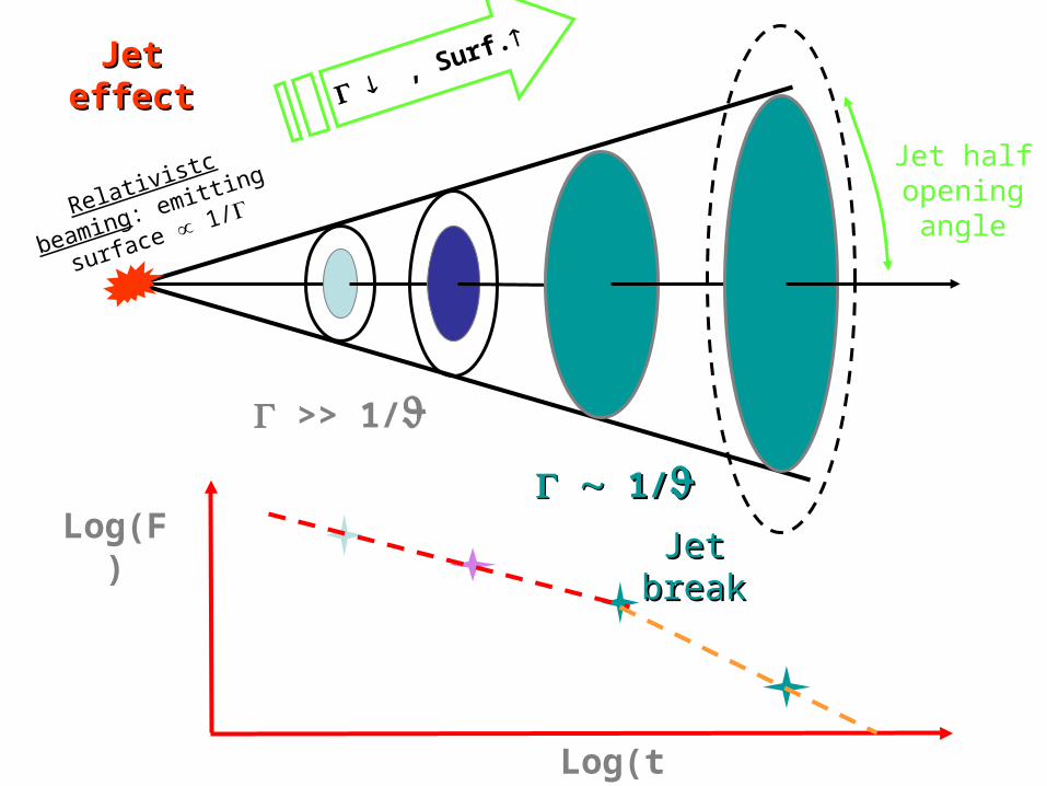
Jet half opening

angle

Jet effectJet effect ,

Surf.

Relativistc beaming:

emitting surface

1/

1/1/

Log(t)

Log(F)

Jet Jet breakbreak

>> 1/

X-ray Flashes and X-ray Rich Bursts

• XRFs prompt emission spectrum peaks at energies tipically one order of magnitude lower than those of GRBs.

XRFs empirically defined by a greater fluence in the X-ray band (2-30keV) than in the γ-ray band (30-400keV).

• XRR are an intermediate class between XRFs and GRBs

Why GRBs are so studied for the correlations?

GRBs are extremely energetic events and are expected to

be visible out to z ~ 15-20 (Lamb & Reichart, 2000, ApJ,

536, 1), which is further than that obtainable by quasars

(zmax ~ 6). GRB z ~ 6.7 (Tagliaferri et al. 2005)

Potential use of GRBs to derive an extended z Hubble-

diagram.

Am

ati

et

al.

2002

Am

ati

et

al.

2002

9+2 BeppoSAX GRBs

EE peak

peak

E E

iso

iso

0.5

0.5

Peak energy – Isotropic energy Peak energy – Isotropic energy CorrelationCorrelation

EEp

eak

peak(1

+z

(1+

z))

+ 21 GRBs+ 21 GRBs (Batse, Hete-II, Integral)

Gh

irla

nd

a,

Gh

isellin

i, L

azz

ati

20

04

Gh

irla

nd

a,

Gh

isellin

i, L

azz

ati

20

04

Am

ati

20

06

(m

ost

recen

t u

pd

ate

)A

mati

20

06

(m

ost

recen

t u

pd

ate

)

EE peak

peak

E E

iso

iso

0.5

0.5

XX22 =

357/

28

=35

7/28

EEp

eak

peak(1

+z

(1+

z))

EEisoiso

Nava e

t al.

2006;

Gh

irla

nd

a e

t al.

2007

Nava e

t al.

2006;

Gh

irla

nd

a e

t al.

2007

“Am

ati”

(62)

“Ghi

rlan

da”

(25)

1- cos 1- cos jetjet

Why is the Ghirlanda relation, Eg (Epeak) 1.5, different from the Amati relation, Eiso Epeak 0.5 ? Because of the correction of

the beaming angle

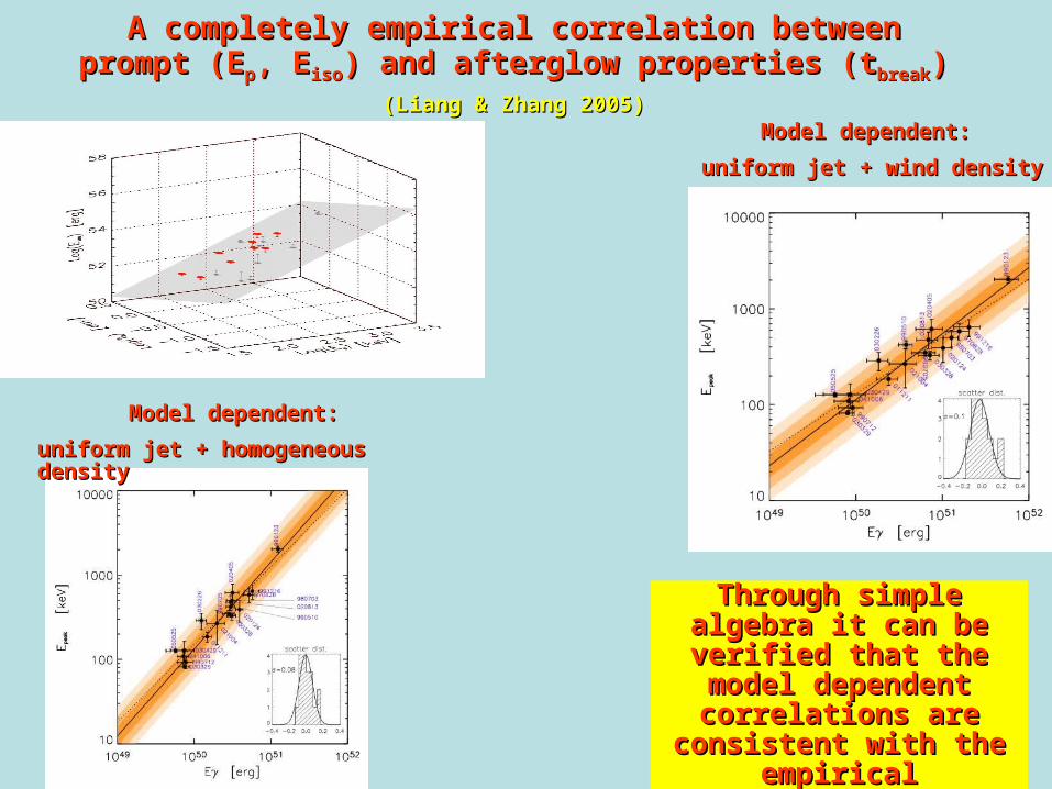
Model dependent: Model dependent:

uniform jet + homogeneous uniform jet + homogeneous densitydensity

Model dependent: Model dependent:

uniform jet + wind densityuniform jet + wind density

Through simple Through simple algebra it can be algebra it can be verified that the verified that the

model dependent model dependent correlations are correlations are

consistent with the consistent with the empirical correlation! empirical correlation!

(Nava et al. 2006)(Nava et al. 2006)

A completely empirical correlation between A completely empirical correlation between prompt (Eprompt (Epp, E, Eisoiso) and afterglow properties (t) and afterglow properties (tbreakbreak))

(Liang & Zhang 2005)(Liang & Zhang 2005)

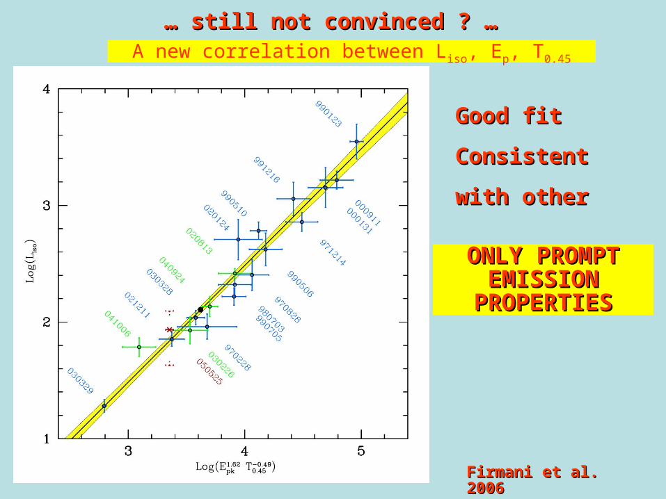
… … still not convinced ? …still not convinced ? …

Good fitGood fit

ConsistentConsistent

with other with other ccoorrrr

Firmani et al. Firmani et al. 20062006

ONLY PROMPT ONLY PROMPT EMISSION EMISSION

PROPERTIESPROPERTIES

A new correlation between Liso, Ep, T0.45

Pir

o a

str

o-p

h/0

001436

Pir

o a

str

o-p

h/0

001436

A lot of kinetic energy should remain to power the afterglowA lot of kinetic energy should remain to power the afterglow

SAX X-ray SAX X-ray afterglow afterglow light curvelight curve

PromptPrompt

The study of prompt vs afterglow

A further step to build LX –Ta relation

EEafterglowafterglow < E < Epromptprompt

EE afterg

low

afterg

low ~

0.1 E

~ 0.1 E pro

mpt

prompt

Flux vs observed timeFlux vs observed time

=0.48=0.48

Nard

ini et

al.

2006

Nard

ini et

al.

2006

Luminosity vs rest frame timeLuminosity vs rest frame time

=0.28=0.28

Nard

ini et

al.

2006

Nard

ini et

al.

2006

Clustering of the optical Clustering of the optical luminositiesluminosities

GRB – Afterglow – Temporal GRB – Afterglow – Temporal PropertiesProperties

GRB multiwavelength GRB multiwavelength emissionemission

Panaitescu & Kumar

No corr.No corr.

LX-Eg correlate in optical and in X?

The X-ray luminosities are more widely used for testing

correlations

We also choosed X-ray luminosity for our analysis

• to find a relation involving an observable property to standardize GRBs

• in the same way as the Phillips law with SNeIa

Why we are searching a new correlation?

The sample

• 17 GRBs with 0.0085< z<1.949 (Swift, BeppoSAX, Integral)

Ltotal = Cg(t) = kh(t) + atb = L1 + L2 (1)

g(t) is the temporal shape of the whole lightcurve

h(t) t< tstart g(t)= atb

start t > tstart

For g(tstart) = atbstart =kh(tstart)

Integrating 1)

Normalization • • C=Etot

o

tot dttgCE )(1)(

o

dttg

Focusing on L2

• L2=

Linearization provides a visual evidence of the claimed model and it gives the quantities as logarithms ready to compute the distance moduli

Linear fits are used to find parameters also of other models which can be

linearized through a suitable transformation of the variables.

Non-linear least-squares (NLLS) Marquardt-Levenberg algorithm, .a and b computed by the fit.

Values for -1.17 < b < -1.91

bat tbaL logloglog

y

y

x

x

Time rescaled to restframe

The tbreak of the lightcurve is highly variable 103<tstart<104s

bstarttL The Spearman coefficient of

correlation is 0.75

How can we improve it?

Increasing the statistic of GRBs observed by the same instruments to see if there is a selection effect depending on the instruments and improving the statistical method

We used Ta and Fa values computed through Willingale et al. 2007 of the

afterglow and the D’Agostini method as statistical method.

The correlation is new because it involves only the afterglow quantities

Willin

gale

et

al.

W

illin

gale

et

al.

2007

2007

SWIFTSWIFT

ac

cctTt

(Tc, Fc) is the transition between the exponential and the power law

αc the time constant of the exponential decay, Tc/αc

•tc marks the initial time rise and the time of maximum flux occurring atc

cctTt

In most cases ta=Tp.

No case in which the two componets were sufficiently separated such that this time could

be fitted as a free parameter. We are unable to see the rise of the afterglow component because the prompt

component always dominates at early times and ta could be much less than Tp for

most GRBs.

The phenomenological formula

)exp(t

t

T

tF a

aa

a

)/()/( ttTtp

pppp eeF

• 1)f_c(t) = f_p(t) + f_a(t)

• 2)f_p(t)=

• fa(t)=

Willingale at al. 2007

For t<Ta

aTt

Negligible if ta=0 and in that case we

return to the simple case of power

law decay

General treatment

3) Lbol = 4 πDL2 (z) P bol

max

min

)(

)(1/10000

1/1E

E

zkeV

zkeVbolo

dEEE

dEEE

PP

Pbolo is the bolometric flux, while P is the peak flux,

Emin-Emax is the energy range in which P occurs

f(t)=f (Ta)=fa(Ta)

3) LX(Ta) = 4 πDL 2(z) FX(Ta)=aTab

We compute the X-ray luminosities at the time Ta so that we have to set

Since the contribution on the prompt component is typically

smaller than the 5%,

Much lower than the statistical uncertainty on Fa(Ta).

Neglecting Fp(Ta) we reduce the error on Fx(Ta) without

introducing any bias.

E_min, E_max = (0.3, 10) keV set by the

instrument bandpass

max

min

)(

)(

)(

1max/

1min/E

E

zE

zEX

dEEE

dEEE

tfF

• Due to the limited energy range, the GRB spectrum may be described by a simple

• power law

• β(t)

• βp for the prompt phase

• βpd for the prompt decay

• βa for the plateau observed at the time Ta

• βad for the afterglow at t > Ta

We estimate βa because we compute Fx(Ta)

EE )(

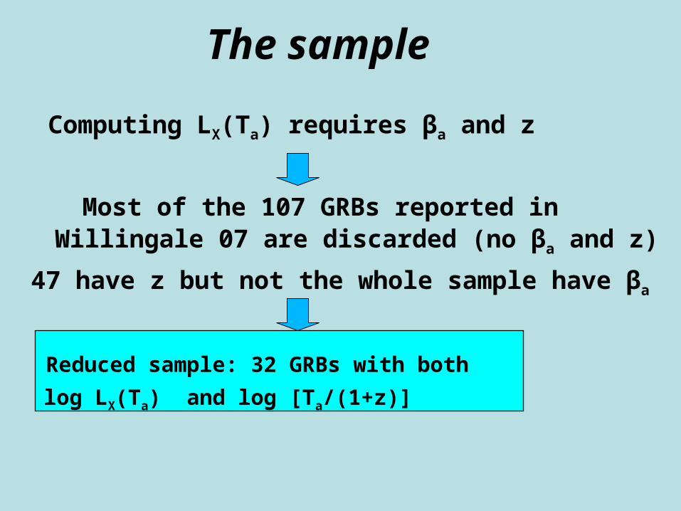
The sample

Computing LX(Ta) requires βa and z

Most of the 107 GRBs reported in Willingale 07 are discarded (no βa and z)

47 have z but not the whole sample have βa

Reduced sample: 32 GRBs with both

log LX(Ta) and log [Ta/(1+z)]

baTL

log t a

golL

Sample of 32 GRBsbaTL

The computations errors

• the parameters of interest are given with their 90%confidence ranges.

• Following Willingale (priv. comm.), we have assumed independent Gaussian

• errors and obtained 1 sigma uncertainties by roughly dividing by 1.65 the 90% errors.

Important remark

• The presence of the luminosity distance in the equation 1)

DL(z) = (c/H0) dL(z)

dL(z)=(1+z)

constrain us to adopt a cosmological model

to compute Lx(Ta)

• with (ΩM,h)=(0.291, 0.697)

(ΛCDM)

z

MM z

dz

03 )1()'1(

'

The program to compute dl• ΩM=0.291• h0=0.697*100• c=300000• Mpc=3.08*10^(24)

DLz : 1 z NIntegrate1 Sqrt 1 t ^3 1 , t, 0, z name ReadList"directorynamegrbname.txt", TableString, 1 name Partname, All, 1z ReadList"directorynamegrbz.txt", Table Number, 1 z Partz, All, 1Fori 1, i 107, i , Printname i , " z", z i , " DL", Mpc^2 c h0 DLz i ^2

• L and Ta • measurement errors :σL, σTa

• statistical uncertainties on log(L), log(Ta) :

• (σL)/L *(1/ln(10) , (σTa)/Ta *(1/ln(10) respectively.

• These errors may be comparable so that it is not possible to decide what is the independent variable to be used in the usual χ2 fitting analysis.

• Moreover, the relation L = a Tab may be affected by an intrinsic

• scatter σint of unknown nature that has to be taken into

• account.

• to determine the parameters (a, b, σint)

• a Bayesian approach D’agostini 05 thus maximizing the likelihood function

• L(a, b, σint) = exp (-L(a, b, σint).

The error computations

The D’Agostini Method

In more details

• Computation of the error on Ta taking into account of the not simmetric errors

• σTa= logTa+ (σ MaxlogTa –logTa)+(logTa- σMinlogTa)/1.65

• The error on Lx(Ta) that is computed with the error propagations rules, taking intio account of F(Ta), Ta and Tp and βa

0 in the case of simmetric error

The likelihood

• whose maximization is performed in the two parameter space (b, σint) since a may be estimated analytically

• so that we will not consider it anymore as a fit parameter.

• (a, b, σint) = (48.54, -0.74, 0.43)

The goodness of the fit

Defining the best fit residuals as

δ = yobs – yfit, < δ>=-0.08

δ does not correlate with the other parameters of the fitted

flux

Sperman correlation coefficient r =-0.23 between and δ

and z favours no significative evolution of the Lx - Ta

relation with the redshift ( in the exercise you will do the

same but simply beetwen Lx-z and Ta-z)

δ rms = 0.52

The comparison between the statistical methods

• the best fit obtained through a Levemberg Marquardt algorithm with 1.5 σ outliers rejection

• (a, b) = (48.58, -0.79)

in good agreement with the below maximum likelihood estimator results are independent on the fitting method

(a, b, σint) = (48.54, -0.74, 0.43).

• since the Bayesian approach is better motivated and also allows for an intrinsic scatter, we hereafter elige this as our preferred technique.

• (but you will use in the excercise for semplicity the Levemberg Marquardt algorithm)

solid lines D’Agostini method

dashed lines Levemberg-Marquardt estimator

Best fit curves

Attempting to reduce σint

Higher best fit residuals are obtained for GRBs with luminosities smaller than Lx>1045 erg and time parameter log (Ta/(1+z)) < 5

Repeating the above analysis using only 28 out of 32 GRBs.

GRB sample with 28 GRBs

Lx>10^45 erg

(Ta/(1+z)) < 5

The discarded GRBs

GRB050824, GRB060115

GRB060607A, GRB060614

• While the first two appear to be unaffected by any problem, for the latter two, the data cover less than 50% of the T90 range

• For GRB060607A, the prompt component dominates over the afterglow

f(Ta) = fa(Ta) is not valid anymore.

• Two parameters correlation

• A small scatter compared to the other correlation

• Well defined quantities involved Lx(Ta) and Ta

• A good sample

• No evolution with redshift

• Lx(Ta) is not an observable!

Disavantage

Advantages

Found a linear relation

Log[LX(Ta)] vs log [Ta/(1+z)]

Intrinsic scatter int = 0.33

comparable to previously reported relations.

RESULTS

(a, b) = (48.09, -0.58)

HOW TO FIND THE LIGHTCURVES AND SPECTRA

http://www.swift.ac.uk/xrt_spectra/00100585/

http://www.swift.ac.uk/xrt_curves/00100585/

The temporal decays parameters corresponding to a certain time region and the spectral decay ones are in the following papers

arXiv.org > astro-ph > arXiv:0812.3662v1

arXiv.org > astro-ph > arXiv:0812.4780v1

arXiv.org > astro-ph > arXiv:0704.0128v2

The first part of the excercise

• Make a table of all GRBs with known redshift and observed in the X-ray energy range.

• Missions :

• Swift (0.3-10 keV), • Integral(3-35keV), • Chandra (50eV-10keV),• XMM (0.1-15keV),• SuperAgile(18-60 keV),• Beppo Sax(0.1-10keV), • Hete2 (1-25keV),• Konus (10-770keV)

• Xrange goes from 0.1-120 keV soft X• Hard X from 80keV-1000keV