Stephen F. Austin State University SFA ScholarWorks eBooks 2011 Basic Concepts in Forest Valuation and Investment Analysis Steven H. Bullard Stephen F. Austin State University, Arthur Temple College of Forestry and Agriculture, [email protected] omas J. Straka Clemson University, [email protected] Follow this and additional works at: hp://scholarworks.sfasu.edu/ebooks Part of the Agribusiness Commons , Finance and Financial Management Commons , Forest Management Commons , and the Other Forestry and Forest Sciences Commons Tell us how this article helped you. is Book is brought to you for free and open access by SFA ScholarWorks. It has been accepted for inclusion in eBooks by an authorized administrator of SFA ScholarWorks. For more information, please contact [email protected]. Repository Citation Bullard, Steven H. and Straka, omas J., "Basic Concepts in Forest Valuation and Investment Analysis" (2011). eBooks. Book 21. hp://scholarworks.sfasu.edu/ebooks/21

Welcome message from author
This document is posted to help you gain knowledge. Please leave a comment to let me know what you think about it! Share it to your friends and learn new things together.
Transcript
Stephen F. Austin State UniversitySFA ScholarWorks
eBooks
2011
Basic Concepts in Forest Valuation and InvestmentAnalysisSteven H. BullardStephen F. Austin State University, Arthur Temple College of Forestry and Agriculture, [email protected]
Thomas J. StrakaClemson University, [email protected]
Follow this and additional works at: http://scholarworks.sfasu.edu/ebooks
Part of the Agribusiness Commons, Finance and Financial Management Commons, ForestManagement Commons, and the Other Forestry and Forest Sciences CommonsTell us how this article helped you.
This Book is brought to you for free and open access by SFA ScholarWorks. It has been accepted for inclusion in eBooks by an authorized administratorof SFA ScholarWorks. For more information, please contact [email protected].
Repository CitationBullard, Steven H. and Straka, Thomas J., "Basic Concepts in Forest Valuation and Investment Analysis" (2011). eBooks. Book 21.http://scholarworks.sfasu.edu/ebooks/21

$$in
Forest Valuationand
Investment Analysis
Basic Concepts
in
Forest Valuationand
Investment Analysis
S.H. Bullard • T.J. Straka
Section 3. Twelve formulas – page 3.2
3.1 Introduction (continued)
The overall pattern we use for decision tree development follows a diagram presented by J.E. Gunter and H.L. Haney, 1978, “A Decision Tree for Compound Interest Formulas,” South. J. Appl. For. 2(3):107.
In Section 3 we develop a “decision tree” diagram for selecting among 12 compound interest formulas. The diagram is actually a composite of three diagrams, however, based on what you’re calculating …
Present Valueor
Future Value
Payments
To calculate …
Interest Rate orNumber of Periods
Present Value and Future Value Formulas
Six Present and Future Valueformulas are developed and applied
in Section 3.2
12 Formulas in 3 Groups
Payment Formulas
Four payment formulas are developedand applied in Section 3.2
Formulas for “i” and “n”
Two formulas developed and appliedin Section 2 are included in the
12-formula decision tree diagramin Section 3.4
In Section 3 we present exam-ples for each formula discussed. We also provide problems, however, and we strongly encourage readers to “put their pencil to paper.” Solutions to all problems are in Section 10.
In Section 3.2 we develop and apply six formulas for Present and Future Value, and in Section 3.3 we develop and apply four formulas for payments. Each of these formula “groups” is developed and presented using a decision tree diagram for formula selection. In Section 3.4 we present a complete dia-gram for compound interest formulas that includes these two groups of for-mulas, plus a third group comprised of two formulas developed and applied in Section 2.
Basic Concepts
S.H. Bullard • T.J. Straka
Basic Concepts in
Forest Valuation and Investment Analysis
Edition 3.0
by
Steven H. BullardArthur Temple College of Forestry and Agriculture
Stephen F. Austin State UniversityNacogdoches, Texas
and
Thomas J. StrakaDepartment of Forestry and Natural Resources
Clemson UniversityClemson, South Carolina
Distributed byForestry Suppliers, Inc., Jackson, MS
www.forestry-suppliers.com
Copyright © 2011 Edition 3.0 Bullard–StrakaISBN 0-9641291-2-4

This book was originally intended to supplement lectures in forestry eco-
nomics at the undergraduate level. It’s currently used for that purpose in
‘Forest Resource Economics’ courses at several universities. The book is also
intended, however, to serve as a basic reference for foresters with experience
in valuation and investment analysis concepts and methods. It has proven to
be a valuable resource in forest valuation and investment analysis workshops
for practicing foresters, landowners, and others interested in forestry invest-
ments.
The workbook’s contents, organization, and other characteristics reflect its
purpose as a classroom/workshop supplement and a basic reference.
The book’s emphasis is very applied, and examples and problems are used
to reinforce the concepts presented. As Oliver Wendell Holmes said in The
Autocrat of the Breakfast Table (1858), “Knowledge and timber shouldn’t be
used much till they are seasoned.” To help in “seasoning” their knowledge,
readers are encouraged to put their pencils to paper in working the book’s
examples and problems; solutions to all of the book’s numbered problems
are included in Section 10. Extra problem sets may be used by instructors, of
course, to build on the basics with applications that are most relevant to their
students.
Several topics have been omitted due to orientation. Albert Einstein once
remarked that “Everything should be as simple as possible, but not simpler.”
This phrase describes our approach in preparing this workbook. We’ve omit-
ted from this Edition formulas for gradient series and other complex cash
flows, and formulas for terminating periodic series are discussed only in Sec-
tion 9. Review for the Registered Forester exam. In most applications, their
actual usefulness is limited if the single-sum formulas are well-understood, or
if computer programs are used.
Preface
Purpose
Characteristics
iii
Finally, this book doesn’t include tables of compounding and discounting fac-
tors. Calculators with the yx key are readily available, and interest rates today
are often stated in non-integer form. A calculator with a yx key is needed to
work the book’s examples and problems; a financial calculator may be used,
of course, but isn’t required.
In a publication of this length and type, many decisions are necessary about
the subjects and examples to include, and about the appropriate depth of dis-
cussion and illustration. To help ensure that future editions of this book are
as useful and relevant as possible, therefore, the authors sincerely invite stu-
dents, instructors, and other readers to comment on aspects they find helpful
as well as areas that should be added, deleted, or revised.
S.H. Bullard, DeanArthur Temple College of Forestry and Agriculture
Stephen F. Austin State UniversityP.O. Box 6109, SFA Station
Nacogdoches, TX 75962–6109
T.J. Straka, ProfessorDepartment of Forestry and Natural Resources
Clemson UniversityBox 340317
Clemson, SC 29634–0317
Revision
iv
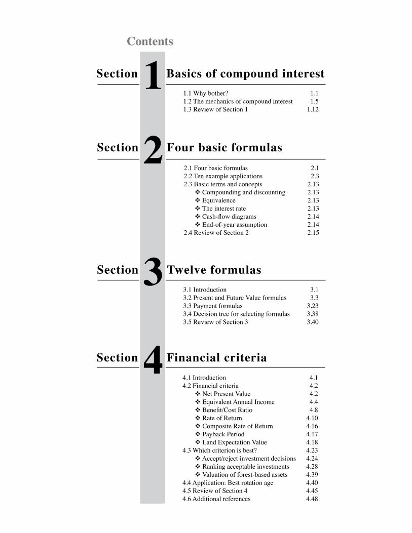
Section Basics of compound interest1.1 Why bother? 1.11.2 The mechanics of compound interest 1.51.3 Review of Section 1 1.12
Section Four basic formulas2.1 Four basic formulas 2.12.2 Ten example applications 2.32.3 Basic terms and concepts 2.13 v Compounding and discounting 2.13 v Equivalence 2.13 v The interest rate 2.13 v Cash-flow diagrams 2.14 v End-of-year assumption 2.142.4 Review of Section 2 2.15
Section Twelve formulas3.1 Introduction 3.13.2 Present and Future Value formulas 3.33.3 Payment formulas 3.233.4 Decision tree for selecting formulas 3.383.5 Review of Section 3 3.40
Section Financial criteria4.1 Introduction 4.14.2 Financial criteria 4.2 v Net Present Value 4.2 v Equivalent Annual Income 4.4 v Benefit/Cost Ratio 4.8 v Rate of Return 4.10 v Composite Rate of Return 4.16 v Payback Period 4.17 v Land Expectation Value 4.184.3 Which criterion is best? 4.23 v Accept/reject investment decisions 4.24 v Ranking acceptable investments 4.28 v Valuation of forest-based assets 4.394.4 Application: Best rotation age 4.404.5 Review of Section 4 4.454.6 Additional references 4.48
Contents
2
1
3
4
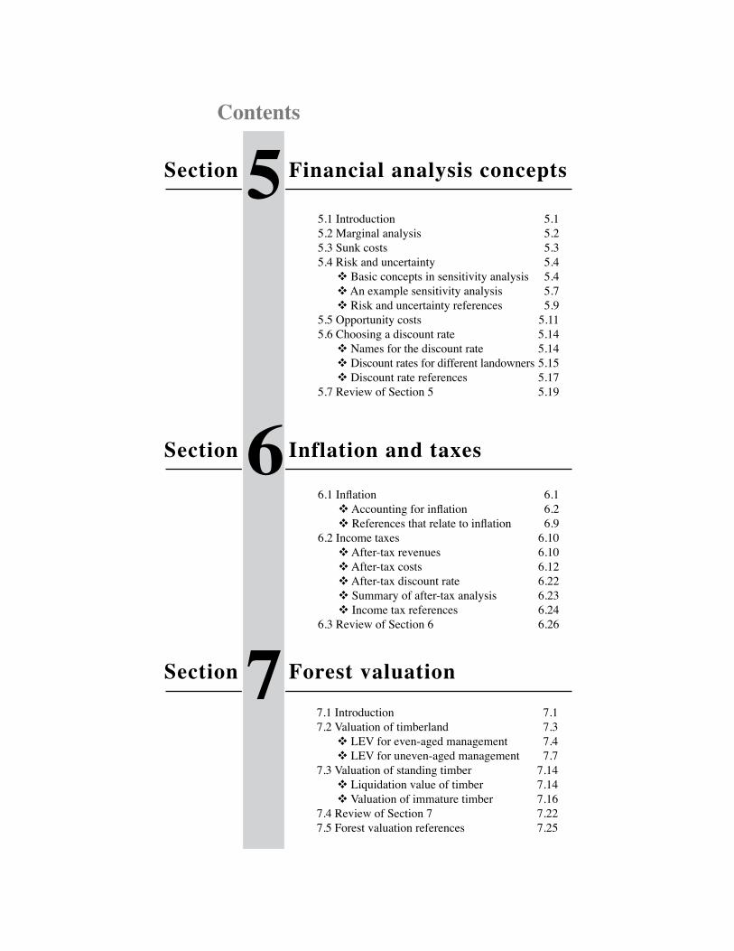
Section Financial analysis concepts
Section Inflation and taxes
Section Forest valuation
7.1 Introduction 7.17.2 Valuation of timberland 7.3 v LEV for even-aged management 7.4 v LEV for uneven-aged management 7.77.3 Valuation of standing timber 7.14 v Liquidation value of timber 7.14 v Valuation of immature timber 7.167.4 Review of Section 7 7.227.5 Forest valuation references 7.25
Contents
5.1 Introduction 5.15.2 Marginal analysis 5.25.3 Sunk costs 5.35.4 Risk and uncertainty 5.4 v Basic concepts in sensitivity analysis 5.4 v An example sensitivity analysis 5.7 v Risk and uncertainty references 5.95.5 Opportunity costs 5.115.6 Choosing a discount rate 5.14 v Names for the discount rate 5.14 v Discount rates for different landowners 5.15 v Discount rate references 5.175.7 Review of Section 5 5.19
6.1 Inflation 6.1 v Accounting for inflation 6.2 v References that relate to inflation 6.96.2 Income taxes 6.10 v After-tax revenues 6.10 v After-tax costs 6.12 v After-tax discount rate 6.22 v Summary of after-tax analysis 6.23 v Income tax references 6.246.3 Review of Section 6 6.26
5
6
7
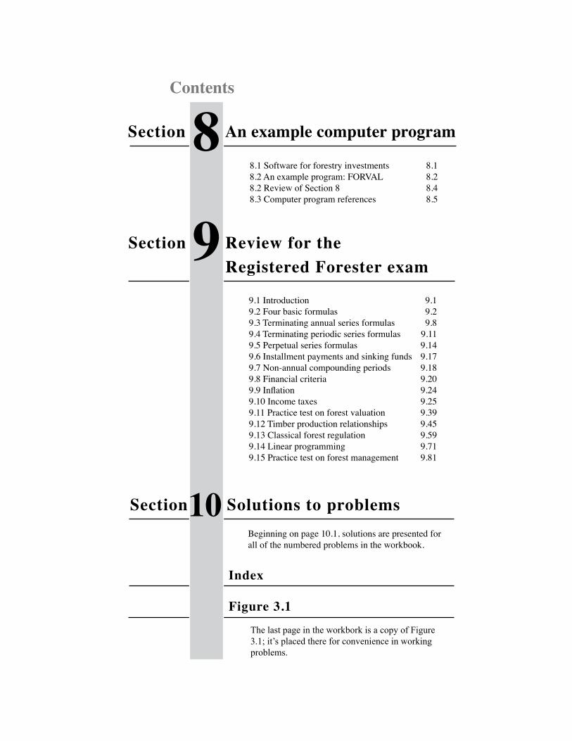
Section An example computer program
Section Review for the
Section Solutions to problemsBeginning on page 10.1, solutions are presented for all of the numbered problems in the workbook.
Contents
8.1 Software for forestry investments 8.18.2 An example program: FORVAL 8.28.2 Review of Section 8 8.48.3 Computer program references 8.5
9.1 Introduction 9.19.2 Four basic formulas 9.29.3 Terminating annual series formulas 9.89.4 Terminating periodic series formulas 9.119.5 Perpetual series formulas 9.149.6 Installment payments and sinking funds 9.179.7 Non-annual compounding periods 9.189.8 Financial criteria 9.209.9 Inflation 9.249.10 Income taxes 9.259.11 Practice test on forest valuation 9.399.12 Timber production relationships 9.459.13 Classical forest regulation 9.599.14 Linear programming 9.719.15 Practice test on forest management 9.81
Registered Forester exam
Index
Figure 3.1
The last page in the workbork is a copy of Figure 3.1; it’s placed there for convenience in working problems.
8
9
10

Section 1. Basics of compound interest – page 1.1
Section
1 Basics ofcompound interest
1.1 Why bother? 1.11.2 The mechanics of compound interest 1.51.3 Review of Section 1 1.12
“An understanding of the economics of capital in forestry is, of all things that you may get from this book, possibly the most essential and useful to you as a
forester.”– W.A. Duerr, Forestry Economics (1960)
Why is an understanding of the “economics of capital in forestry essential and useful to you as a forester?” Why should foresters bother learning the basics of compound interest or the application of financial criteria like “Net Present Value” and “Rate of Return?”
To begin understanding why foresters should be able to apply these concepts, con-sider the number and variety of applications in forestry – all of the examples on the next page can be addressed with compound interest techniques. In each example, volumes, dollar values, and population numbers are involved that occur at different points in time. Their time value must be considered.
1.1 Why bother?
Page
Consider the number of important applications in forestry …
1. Basics of compound interest
2. Four basic formulas
3. Twelve formulas
4. Financial criteria
5. Financial analysis concepts
6. Inflation and taxes
7. Forest valuation
8. An example computer program
9. Review for the Registered
Forester exam
10. Solutions to problems
Section 1. Basics of compound interest – page 1.2
1.1 Why bother? (continued)
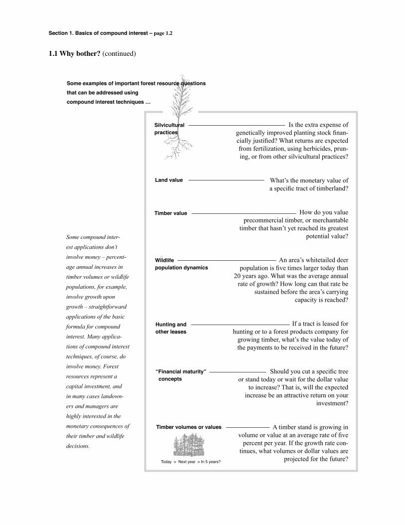
Is the extra expense ofgenetically improved planting stock finan-cially justified? What returns are expected from fertilization, using herbicides, prun-ing, or from other silvicultural practices?
What’s the monetary value ofa specific tract of timberland?
How do you valueprecommercial timber, or merchantable
timber that hasn’t yet reached its greatest potential value?
An area’s whitetailed deerpopulation is five times larger today than
20 years ago. What was the average annual rate of growth? How long can that rate be
sustained before the area’s carrying capacity is reached?
If a tract is leased forhunting or to a forest products company for
growing timber, what’s the value today of the payments to be received in the future?
Should you cut a specific treeor stand today or wait for the dollar value
to increase? That is, will the expected increase be an attractive return on your
investment?
A timber stand is growing involume or value at an average rate of five
percent per year. If the growth rate con-tinues, what volumes or dollar values are
projected for the future?
Some examples of important forest resource questionsthat can be addressed usingcompound interest techniques …
Silviculturalpractices
Land value
Timber value
Wildlifepopulation dynamics
Hunting andother leases
“Financial maturity” concepts
Timber volumes or values
Some compound inter-
est applications don’t
involve money – percent-
age annual increases in
timber volumes or wildlife
populations, for example,
involve growth upon
growth – straightforward
applications of the basic
formula for compound
interest. Many applica-
tions of compound interest
techniques, of course, do
involve money. Forest
resources represent a
capital investment, and
in many cases landown-
ers and managers are
highly interested in the
monetary consequences of
their timber and wildlife
decisions.
Today > Next year > In 5 years?
Section 1. Basics of compound interest – page 1.3
It’s important to “bother” learning to apply compound interest in forest valua-tion and investment analysis because there are so many important applications. Two characteristics of forests give rise to the number of applications; they make it extremely important for forestry decision makers to accurately account for the “time value” of money:
• The time period involved… Decisions that affect forests and other natural resources almost always
involve values that occur at different points in time, and these time periods can be very long compared to many investments.
• The amount of capital involved… Decisions concerning forestry investments often involve significant
amounts of capital. Merchantable timber alone, for example, may rep-resent a capital investment worth thousands of dollars per acre.
There are many applications of compound interest techniques in forest valua-tion and investment analysis, but why should foresters bother learning to apply these techniques? Why not rely on published reports that specify the rate of return earned on different types of forestry investments, for example, rather than learning to estimate such returns on a case-by-case basis? The answer is because forest lands and forest landowners are inherently diverse; because of this diversity, forest valuation and investment analysis questions must often be addressed on a tract-by-tract and landowner-by-landowner basis. Timber prices, costs, and other factors may also vary greatly over time and for different geographic areas.
Applications are most relevant when they are for specific tracts, specific owners, and a given time and place.Generalizations about forestry investments are often of limited use because forest properties vary, because forest landowners differ in very important ways, and because prices, costs, and other values are often valid only for a specific time period and geographic area.Properties differ… • Stand characteristics such as timber species, volume, and quality vary
widely from tract to tract. • Forest properties vary in site quality, as well as in accessibility, loca-
tion, and other factors that affect timber and other monetary values.Landowners differ… • Management objectives vary with ownership. • The rate of return considered acceptable for timberland investments is
landowner-specific.Prices, costs, and other values vary over time and by region … • Many factors cause timber prices, land values, and other variables to
change over time, and to vary significantly by geographic area.
1.1 Why bother? (continued)
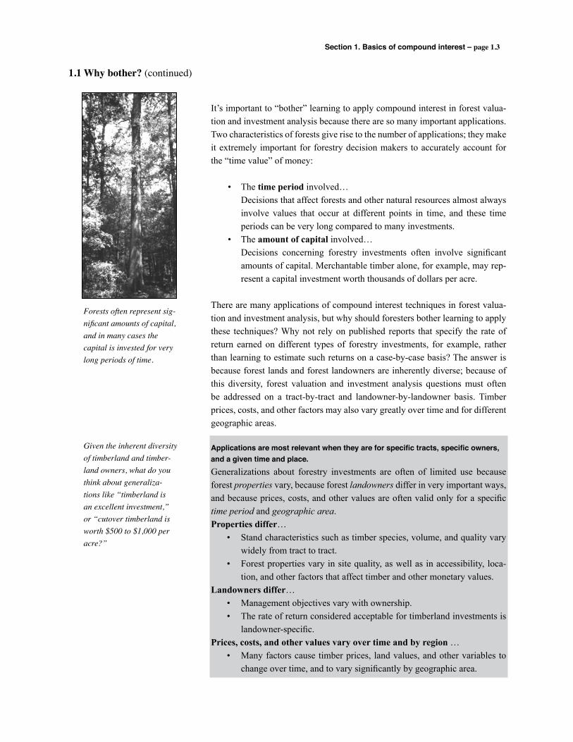
Forests often represent sig-nificant amounts of capital, and in many cases the capital is invested for very long periods of time.
Given the inherent diversity of timberland and timber-land owners, what do you think about generaliza-tions like “timberland is an excellent investment,” or “cutover timberland is worth $500 to $1,000 per acre?”
Section 1. Basics of compound interest – page 1.4
1.1 Why bother? (continued)
There are other important reasons why we should understand compound inter-est and its use in today’s society, reasons that have nothing to do with forest resources or potential timber investments. As consumers and producers in modern society, we regularly encounter compound interest applications:
• Bank accounts • Home mortgage payments • Personal investment decisions • Car and truck financing • Credit card accounts
Banks and other financial institutions use the same formulas and methods described in this workbook, and therefore many of the compound interest tech-niques and concepts we discuss apply to decisions about new cars and financial planning, as well as to decisions about forest-based assets. Monthly payments, for example, are calculated using the same formula, whether the money is bor-rowed for a car, a house, a feller buncher, or a tree planter.
Other reasons to “bother”with compound interest …
What are some other applications of compound interest?
Section 1. Basics of compound interest – page 1.5
Would you prefer to receive $100 today, or would you rather wait and receive the $100 five years from now? Most of us would choose to have the money as soon as possible, even if there is absolutely no risk or uncertainty involved. A dollar we receive or pay today is generally “worth” more to us than a dollar we’re to receive or pay in the future. The dollar has “value” with respect to a specific point in time – the nearer to the present, the higher the dollar’s “value.”
Compound interest allows us to mathematically account for the value of dollars that occur at different points in time. Using an appropriate interest rate, we can calculate dollars that are “equivalent” in value based on a reference year, and we can thus compare choices and make decisions about the use of funds that occur over time.
1.2 The mechanics of compound interest
Money has a “time value”– a dollar today is not the same as a dollar tomorrow.
Compound interest allows us to account for the “time value” of money.
Have you encountered “real world” situations where the time value of money was ignored?
The “total of payments” for a loan is meaningless … One example of ignoring the time value of money is car and truck advertisements that show the “total
of payments.” This “total” is obtained by adding all of the projected payments, even though they occur at different points in time. The total of payments is a meaningless number because the pay-ments’ time value is ignored.
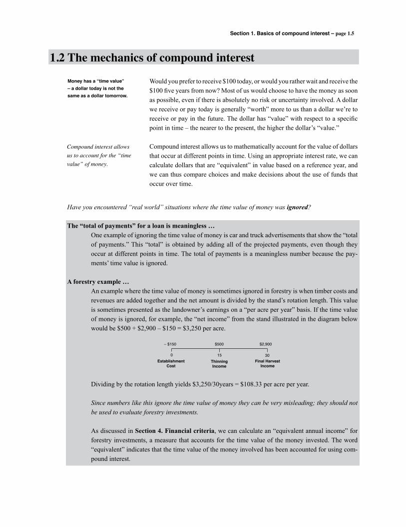
A forestry example … An example where the time value of money is sometimes ignored in forestry is when timber costs and
revenues are added together and the net amount is divided by the stand’s rotation length. This value is sometimes presented as the landowner’s earnings on a “per acre per year” basis. If the time value of money is ignored, for example, the “net income” from the stand illustrated in the diagram below would be $500 + $2,900 – $150 = $3,250 per acre.
Dividing by the rotation length yields $3,250/30years = $108.33 per acre per year.
Since numbers like this ignore the time value of money they can be very misleading; they should not be used to evaluate forestry investments.
As discussed in Section 4. Financial criteria, we can calculate an “equivalent annual income” for forestry investments, a measure that accounts for the time value of the money invested. The word “equivalent” indicates that the time value of the money involved has been accounted for using com-pound interest.
EstablishmentCost
ThinningIncome
Final HarvestIncome
0 15 30
– $150 $500 $2,900

Section 1. Basics of compound interest – page 1.6
1.2 The mechanics of compound interest (continued)
When money is placed in an interest-bearing account, the account value “grows” over time. After one interest-bearing period, for example, an account should have the original deposit (the principal), plus the interest that’s earned on the principal (Figure 1.1).
The account value after one interest-bearing period is therefore:
Account Value After 1 Period = (Principal) + (Interest Earned)
Notice, however, that the interest earned after one period of time is: (Principal) x (Interest Rate)
So the account value after one interest-bearing period is:
Account Value After 1 Period = (Principal) + (Principal) (Interest Rate) = (Principal) (1 + Interest Rate) = (Principal) (1 + i)
A very simple formula will therefore calculate the total amount of money in an interest-bearing account after one period of time:
Account Value After 1 Period = (Principal) (1 + i), where “i” is the interest rate in decimal percent.
If you place $100 into an account for one year at 8% interest, for example, the amount of money in the account after one year is the $100 principal plus $100(.08) = $8 in interest. The total value of the account is:
$100.00 + $100.00(.08) = $108.00
Using the formula above, the total is calculated directly:
$100(1+.08) = $108.
Compound interest increases the amount of money in an account over time …
Timber capital is prin-cipal that’s “banked on the stump.” Over time, a compound rate of interest is earned on this timber “account.”
We develop the basic mechanics of compound interest here in Section 1.2, and we apply the techniques to some example forestry problems in Section 2.
Principal Principal
Interest
Beginning End
Figure 1.1Account value after one interest-bearing period of time.
Account ValueAfter One Period
= Principal + Interest
Section 1. Basics of compound interest – page 1.7
1.2 The mechanics of compound interest (continued)
If the money in an interest-bearing account (principal plus interest) is not withdrawn after the first period, with compound interest, the interest rate is earned on the total amount left in the account for the next time period. This total is essentially “borrowed” again by the interest payer, i.e., for another inter-est bearing period of time. You therefore earn interest on interest (the interest earned during the first period), as well as on the original deposit.
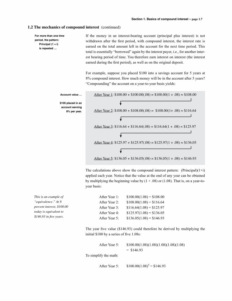
For example, suppose you placed $100 into a savings account for 5 years at 8% compound interest. How much money will be in the account after 5 years? “Compounding” the account on a year-to-year basis yields:
After Year 1: $100.00 + $100.00(.08) = $100.00(1 + .08) = $108.00
After Year 2: $108.00 + $108.00(.08) = $108.00(1+ .08) = $116.64
After Year 3: $116.64 + $116.64(.08) = $116.64(1 + .08) = $125.97
After Year 4: $125.97 + $125.97(.08) = $125.97(1 + .08) = $136.05
After Year 5: $136.05 + $136.05(.08) = $136.05(1 + .08) = $146.93
The calculations above show the compound interest pattern: (Principal)(1+i) applied each year. Notice that the value at the end of any year can be obtained by multiplying the beginning value by (1 + .08) or (1.08). That is, on a year-to-year basis:
After Year 1: $100.00(1.08) = $108.00 After Year 2: $108.00(1.08) = $116.64 After Year 3: $116.64(1.08) = $125.97 After Year 4: $125.97(1.08) = $136.05 After Year 5: $136.05(1.08) = $146.93
The year five value ($146.93) could therefore be derived by multiplying the initial $100 by a series of five 1.08s:
After Year 5: $100.00(1.08)(1.08)(1.08)(1.08)(1.08) = $146.93To simplify the math:
After Year 5: $100.00(1.08)5 = $146.93
For more than one time period, the pattern: Principal (1 + i) is repeated …
Account value …
$100 placed in an account earning
8% per year.
This is an example of “equivalence.” At 8 percent interest, $100.00 today is equivalent to $146.93 in five years.
Section 1. Basics of compound interest – page 1.8
1.2 The mechanics of compound interest (continued)
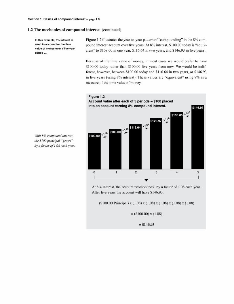
Figure 1.2 illustrates the year-to-year pattern of “compounding” in the 8% com-pound interest account over five years. At 8% interest, $100.00 today is “equiv-alent” to $108.00 in one year, $116.64 in two years, and $146.93 in five years.
Because of the time value of money, in most cases we would prefer to have $100.00 today rather than $100.00 five years from now. We would be indif-ferent, however, between $100.00 today and $116.64 in two years, or $146.93 in five years (using 8% interest). These values are “equivalent” using 8% as a measure of the time value of money.
In this example, 8% interest is used to account for the time value of money over a five year period …
Figure 1.2Account value after each of 5 periods – $100 placedinto an account earning 8% compound interest.
$100.00$108.00
$116.64
$125.97
$136.05
$146.93
x 1.08x 1.08
x 1.08
x 1.08
x 1.08
0 1 2 3 4 5
At 8% interest, the account “compounds” by a factor of 1.08 each year. After five years the account will have $146.93:
($100.00 Principal) x (1.08) x (1.08) x (1.08) x (1.08) x (1.08)
= ($100.00) x (1.08)
= $146.93
With 8% compound interest, the $100 principal “grows” by a factor of 1.08 each year.
Section 1. Basics of compound interest – page 1.9
We’ve now demonstrated that after one interest-bearing period of time, the amount of money in an account paying “i” percent interest will be:
Account Value After 1 Period = (Principal) (1+i).
We’ve also shown that if compound interest will be earned for multiple periods of time, the above pattern is repeated for each of the interest bearing periods. After five periods, for example, the amount in an account paying “i” percent compound interest will be:
Account Value After 5 Periods = (Principal) (1+i)5.
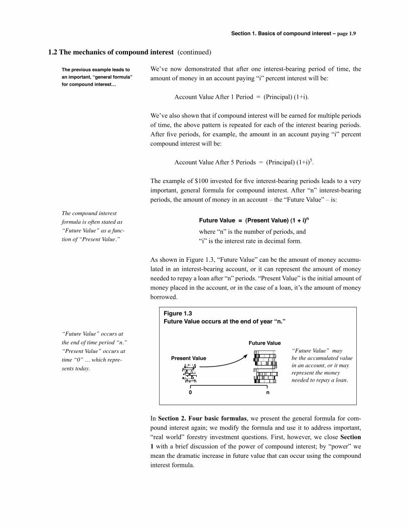
The example of $100 invested for five interest-bearing periods leads to a very important, general formula for compound interest. After “n” interest-bearing periods, the amount of money in an account – the “Future Value” – is:
Future Value = (Present Value) (1 + i)n
where “n” is the number of periods, and “i” is the interest rate in decimal form.
As shown in Figure 1.3, “Future Value” can be the amount of money accumu-lated in an interest-bearing account, or it can represent the amount of money needed to repay a loan after “n” periods. “Present Value” is the initial amount of money placed in the account, or in the case of a loan, it’s the amount of money borrowed.
In Section 2. Four basic formulas, we present the general formula for com-pound interest again; we modify the formula and use it to address important, “real world” forestry investment questions. First, however, we close Section 1 with a brief discussion of the power of compound interest; by “power” we mean the dramatic increase in future value that can occur using the compound interest formula.
1.2 The mechanics of compound interest (continued)
The previous example leads to an important, “general formula” for compound interest…
The compound interest formula is often stated as “Future Value” as a func-tion of “Present Value.”
“Future Value” occurs at the end of time period “n.” “Present Value” occurs at time “0” … which repre-sents today.
Figure 1.3Future Value occurs at the end of year “n.”
Future Value
Present Value
0 n
“Future Value” maybe the accumulated valuein an account, or it mayrepresent the moneyneeded to repay a loan.
Section 1. Basics of compound interest – page 1.10
1.2 The mechanics of compound interest (continued)
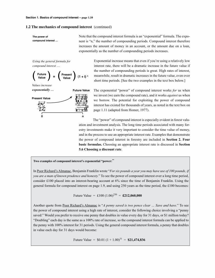
Note that the compound interest formula is an “exponential” formula. The expo-nent is “n,” the number of compounding periods. Compound interest therefore increases the amount of money in an account, or the amount due on a loan, exponentially as the number of compounding periods increases.
Exponential increase means that even if you’re using a relatively low interest rate, there will be a dramatic increase in the future value if the number of compounding periods is great. High rates of interest, meanwhile, result in dramatic increases in the future value, even over short time periods. [See the two examples in the text box below.]
The exponential “power” of compound interest works for us when we invest (we earn the compound rate), and it works against us when we borrow. The potential for exploiting the power of compound interest has existed for thousands of years, as noted in the text box on page 1.11 (adapted from Homer, 1977).
The “power” of compound interest is especially evident in forest valu-ation and investment analysis. The long time periods associated with many for-estry investments make it very important to consider the time value of money, and in the process to use an appropriate interest rate. Examples that demonstrate the power of compound interest in forestry are included in Section 2. Four basic formulas. Choosing an appropriate interest rate is discussed in Section 5.6 Choosing a discount rate.
The power of compound interest …
Future Value
Present Value
0 n
( )FutureValue ( )Present
Value= (1 + i) n
Using the general formula forcompound interest …
Values increaseexponentially …
Two examples of compound interest’s exponential “power:”
In Poor Richard’s Almanac, Benjamin Franklin wrote “For six pounds a year you may have use of 100 pounds, if you are a man of known prudence and honesty.” To see the power of compound interest over a long time period, consider £100 placed into an interest-bearing account at 6% since the time of Benjamin Franklin. Using the general formula for compound interest on page 1.9, and using 250 years as the time period, the £100 becomes:
Future Value = £100 (1.06)250 = £212,060,000
Another quote from Poor Richard’s Almanac is “A penny saved is two pence clear … Save and have.” To see the power of compound interest using a high rate of interest, consider the following choice involving a “penny saved:” Would you prefer to receive one penny that doubles in value every day for 31 days, or $1 million today? “Doubling” each day is the same as a 100% rate of increase, so the compound interest formula can be applied to the penny with 100% interest for 31 periods. Using the general compound interest formula, a penny that doubles in value each day for 31 days would become:
Future Value = $0.01 (1 + 1.00)31 = $21,474,836

Section 1. Basics of compound interest – page 1.11
1.2 The mechanics of compound interest (continued)
Interest is the price we pay to borrow money, or the price we charge others to borrow and use our funds. Today, interest is universally accepted as the price of capital, an asset necessary for production and con-sumption in modern society. It is interesting to note, however, that this has not always been the case in the past. As recently as 1950, for example, Pope Pius XII felt compelled to declare that “bankers earn their living honestly.” This quote is in A History of Inter-est Rates by Sidney Homer (1977, Rutgers University Press ). The book describes the Biblical condemnation
of usury, centuries of controversy and debate, and the eventual acceptance by religious leaders of interest as a just compensation to lenders. Interest was originally accepted as a compensation for loss, however, rather than profit from the use of money – the word is derived from the Latin word interesse – “to be lost.” The rela-tively recent acceptance of the charging of interest is indicated by the fact that not until 1836 did the Holy Office of the Catholic Church declare that “all interest allowed by law may be taken by everyone.”
Of interest …
B.C. © 1992 Creators Syndicate, Inc. By permission of Johnny Hart and Creators Syndicate, Inc.
Interest rates are quoted in “percent,” from the Latin words per (for each) and cent (one hundred). Ten percent, for example, literally means “10 for each hundred.”
A final note “of interest” …
Section 1. Basics of compound interest – page 1.12
1.3 Review of Section 1
Section 1. Basics of compound interest
1.1 Why bother? Foresters should “bother” learning how to use compound interest techniques and how to
apply financial criteria like “present net worth” and “rate of return” because: • There are many important applications in forestry – many of them arise because for-
ests represent relatively long-term investments of significant amounts of capital. • Forest lands and forest landowners are diverse, and applications are therefore most
useful when done on a case-by-case basis. Timber prices, land values, operational costs, and many other factors can change greatly over time, and they can vary signifi-cantly at different locations. Generalizations like “cutover land should sell for $1,000/acre” are of limited use in forestry.
• The financial techniques and concepts used in forest valuation and investment analysis also have many non-forestry applications.
1.2 The mechanics of compound interest Money has a time value, and compound interest techniques allow us to account for differ-
ences in value over time. “Equivalent” dollars can be calculated using a specific interest rate and a specific time period.
The general formula for compound interest is:
Future Value = (Present Value) (1 + i)n
where “n” is the number of periods, and “i” is the interest rate in decimal form.
The general formula is exponential, and compound interest is therefore very “powerful.” Because of the relatively long time periods often involved in forestry, the time value of money should not be ignored. The “power” of compound interest can have a dramatic impact on financial decisions.
Section 2. Four basic formulas – page 2.1
Section
2 Four basic formulas
2.1 Four basic formulas 2.12.2 Example applications 2.32.3 Basic terms and concepts 2.132.4 Review of Section 2 2.15
“Money doesn’t talk, it swears.”– Bob Dylan, It’s Alright, Ma, I’m Only Bleeding (1965)
In Section 1. Basics of compound interest, the general formula for compound interest was developed and presented as:
Future Value = (Present Value) (1 + i)n
Note that this simple, “future value” formula has four variables:
Future Value, Present Value, i – the interest rate, and n – the number of time periods.
We can rearrange the compound interest formula to calculate any one of the four variables in terms of the other three. Simply rearranging this formula yields four basic formulas that are extremely useful in forest valuation and investment analy-sis.
2.1 Four basic formulas
Page
The compound interest formula has four variables. We can therefore rearrange it into four basic formulas …
1. Basics of compound interest
2. Four basic formulas
3. Twelve formulas
4. Financial criteria
5. Financial analysis concepts
6. Inflation and taxes
7. Forest valuation
8. An example computer program
9. Review for the Registered
Forester exam
10. Solutions to problems

Section 2. Four basic formulas – page 2.2
2.1 Four basic formulas (continued)
Future Value = (Present Value) (1 + i)n
The general formula for compound interest, or the “Future Value” formula, is used to “compound” values. We can project the future value of a stand of timber using this formula, for example, or we can estimate future timber prices given the projected annual rate of increase over the next “n” years.
The interest rate or “rate of return” formula is Formula 2.1 rewritten in terms of “i,” the compound rate of interest. It’s used to calculate the rate of return on an investment. “Present Value” may be the amount of money paid for a timber stand, for example, while “Future Value” is the value of the timber “n” years later.
The Future Value formula “compounds” a Present
Value “n” periods into the future.
The Present Value formula “discounts” a Future
Value, one that occurs in year “n,” to the present.
The rate of return formulacalculates the interest rate
earned on an investment over an “n” year period.
“n” is the number of periods necessary for a certain
Present Value to compound to a specific Future Value.
The “Present Value” formula is simply the “Future Value” formula (2.1) rewritten or solved for Present Value. It “discounts” values from the future to the present. If we have an estimate of what a timber stand will be worth when it’s mature, for example, we can use this formula to estimate an equiv-alent value today.
Present Value =Future Value
(1 + i)n
Present Value
Future Valuei = – 1
1 / nForumula 2.3 – “i”
The formula for “n” is obtained by taking the natural logarithm of both sides of Formula 2.1, and solving for “n.” We can use this formula to tell us how long it will take for a tree or a timber stand that has a certain “Present Value” to grow to a specific “Future Value,” assuming a compound rate of increase in value of “i” percent per period.
ln (1 + i)
ln (Future Value / Present Value)n =
Forumula 2.2 – Present Value
Forumula 2.1 – Future Value
Forumula 2.4 – “n”
Section 2. Four basic formulas – page 2.3
The four formulas on page 2.2 are simple and easy-to-use, yet they can help address relatively complex, “real world” problems. The 11 examples that follow demonstrate how useful these basic formulas can be in both forestry and non-forestry applications.
Our purpose in presenting these basic formulas and examples is not so much to demonstrate how useful the formulas are, however. Our actual purpose is to introduce basic terms and concepts like “compounding and discounting,” and hopefully to build readers’ confidence in addressing “real world” questions using compound interest techniques. To help build that confidence, we strongly encourage readers to work each of the following example applications using a hand-held calculator.
There are other formulas that are useful in forest valuation and investment anal-ysis, of course. In Section 3 we present twelve forest valuation and investment analysis formulas – these four plus eight additional formulas – with examples and problems demonstrating their use.
The example applications introduce basic terms and concepts, and help build confidence in solving “real world” problems.
Future Value of a savings account …
2.2 Example applications
The following 11 examples apply the four basic formu-las on page 2.2 …
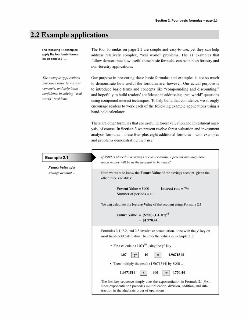
Example 2.1 If $900 is placed in a savings account earning 7 percent annually, how much money will be in the account in 10 years?
Here we want to know the Future Value of the savings account, given the other three variables:
Present Value = $900 Interest rate = 7% Number of periods = 10
We can calculate the Future Value of the account using Formula 2.1:
Future Value = ($900) (1 + .07)10
= $1,770.44
Formulas 2.1, 2.2, and 2.3 involve exponentiation, done with the yx key on most hand-held calculators. To enter the values in Example 2.1:
• First calculate (1.07)10 using the yx key
1.07 yx 10 = 1.9671514
• Then multiply the result (1.9671514) by $900 …
1.9671514 x 900 = 1770.44
The first key sequence simply does the exponentiation in Formula 2.1 first, since exponentiation precedes multiplication, division, addition, and sub-traction in the algebraic order of operations.
Section 2. Four basic formulas – page 2.4
2.2 Example applications (continued)
Example 2.1 on the previous page is an example of compounding. The $900 placed in the savings account is compounded for 10 years using 7% compound interest. In this example, $900 today and $1,770.44 to be received in 10 years are equivalent using a 7% interest rate.
The opposite of compounding is discounting. When we use Formula 2.2 on page 2.2 to calculate a Present Value, given a specific Future Value, we’re discounting, as demonstrated in the next example.
Example 2.1 demonstratescompounding, Example 2.2demonstrates discounting …
Present Value of a standof timber …
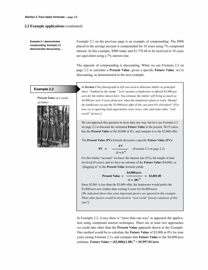
Example 2.2 In Section 1 the photograph at left was used to illustrate timber as principal that’s “banked on the stump.” Let’s assume a landowner is offered $3,000 per acre for the timber shown here. You estimate the timber will bring as much as $4,000 per acre 9 years from now when the landowner plans to retire. Should the landowner accept the $3,000/acre offer if she can earn 8% elsewhere? [For now we’re ignoring land opportunity costs, taxes, risk, and some other “real world” factors.]
We can approach this question in more than one way, but let’s use Formula 2.2 on page 2.2 to discount the estimated Future Value to the present. We’ll calcu-late the Present Value of the $4,000 at 8%, and compare it to the $3,000 offer.
The Present Value (PV) formula discounts a specific Future Value (FV):
For this timber “account” we know the interest rate (8%), the length of time involved (9 years), and we have an estimate of the Future Value ($4,000), so “plugging in” to the Present Value formula yields:
Since $2,001 is less than the $3,000 offer, the landowner would prefer the $3,000/acre now (rather than waiting 9 years for $4,000/acre). [We indicated above that some important factors are ignored in this example. What other factors would be involved in “real world” forestry analyses of this type?]
In Example 2.2, it says there is “more than one way” to approach the applica-tion using compound interest techniques. There are at least two approaches we could take other than the Present Value approach shown in the Example. One method would be to calculate the Future Value of $3,000 at 8% for nine years (using Formula 2.1), and compare that Future Value to the $4,000/acre estimate: Future Value = ($3,000)(1.08) 9 = $5,997.01/acre
PV = (Formula 2.2 on page 2.2) FV
(1 + i) n
Present Value = = $2,001.00$4,000/acre
(1 + .08) 9

Section 2. Four basic formulas – page 2.5
2.2 Example applications (continued)
Since $5,997.01 nine years from now is greater than the $4,000/acre projected stand value, the Future Value approach also shows that receiving $3,000/acre now is preferable to postponing the harvest.
Another way to approach the question in Example 2.2 is to calculate the interest rate you project the stand will earn over the next nine years, and compare that rate to the 8% the landowner can earn elsewhere, as demonstrated in Example 2.3.
The rate of interest earnedon a timber investment …
Example 2.3 The question posed in Example 2.2 can be re-stated:
Should a landowner keep an investment of $3,000/acre “banked on the stump” if it will grow to $4,000/acre in nine years? She can earn 8% on other invest-ments of comparable duration and risk.
An approach to questions of this type that’s popular with foresters and forest landowners is to compare the rate of interest you project the stand will earn to the interest rate that can be earned elsewhere. To be comparable, these rates should be consistent in terms of taxes, inflation, investment duration, and risk.
In this example, the landowner’s present stand value is $3,000/acre, and her projected value in 9 years is $4,000/acre. We can use Formula 2.3 to calculate a projected “rate of return” for her $3,000 per acre capital investment.
To calculate “i” given a Present Value (PV) and a Future Value (FV):
Using the landowner’s values yields:
The $3,000/acre timber “account” is projected to earn a compound interest rate of 3.2% per year over the next 9 years, compared to 8% that can be earned elsewhere.
Examples 2.2 and 2.3 involve a very popular question in forestry: Should you harvest a specific stand of timber now or should you wait? This question is often posed as whether a stand of timber is “financially mature.” This is an important topic in forest management; it’s very briefly described in Section 9. Review for the Registered Forester exam (page 9.6).
i = – 1 (Formula 2.3 on page 2.2) FV
PV
1 / n
i = – 1 = 0.032 (or 3.2%)$4,000
$3,000
1 / 9
Using a hand-held calculator, see if youobtain 0.032 as this problem’s answer.
Example 2.3 is a “simplefinancial maturity”analysis.
Section 2. Four basic formulas – page 2.6
2.2 Example applications (continued)
Examples 2.2 and 2.3 show how useful the basic compound interest formulas can be in addressing important forestry questions. An important concept is also demonstrated by these example applications – very often there is more than one correct way to use compound interest techniques to address a specific forestry investment question. In such cases, the “best” approach is often the one that’s most readily understood by the decision maker.
Deciding when to harvest a particular stand is a very important forestry invest-ment question. Another important type of investment question involves differ-ent silvicultural practices and treatments … Are they financially worthwhile? The next three example applications of the basic compound interest formulas involve intensive cultural practices in pine plantation management:
Are intensive silvicultural practices financially attractive? Example 2.4 … Pruning Example 2.5 … Herbicides for release Example 2.6 … Fertilization
Each of these applications is an example of marginal analysis, since we compare each practice’s marginal costs and marginal benefits.
In many cases there is more than one correct way to analyze a specific forestry investment.
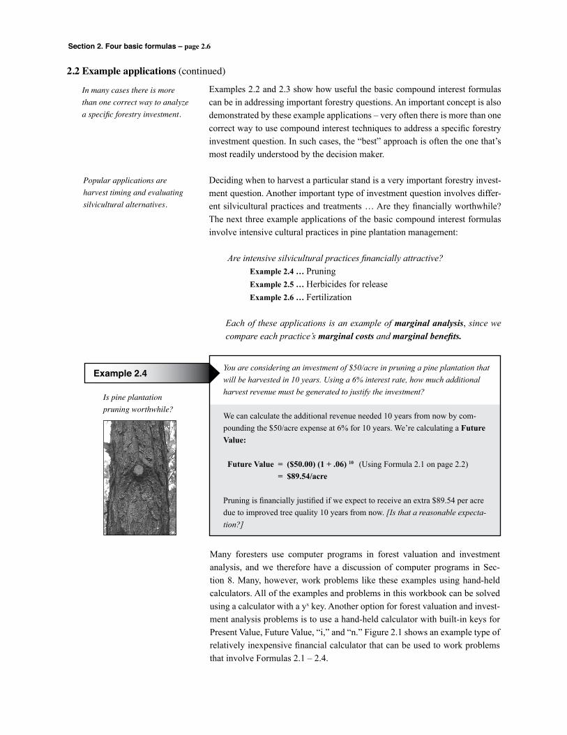
Is pine plantation pruning worthwhile?
You are considering an investment of $50/acre in pruning a pine plantation that will be harvested in 10 years. Using a 6% interest rate, how much additional harvest revenue must be generated to justify the investment?
We can calculate the additional revenue needed 10 years from now by com-pounding the $50/acre expense at 6% for 10 years. We’re calculating a Future Value:
Future Value = ($50.00) (1 + .06) 10 (Using Formula 2.1 on page 2.2) = $89.54/acre
Pruning is financially justified if we expect to receive an extra $89.54 per acre due to improved tree quality 10 years from now. [Is that a reasonable expecta-tion?]
Many foresters use computer programs in forest valuation and investment analysis, and we therefore have a discussion of computer programs in Sec-tion 8. Many, however, work problems like these examples using hand-held calculators. All of the examples and problems in this workbook can be solved using a calculator with a yx key. Another option for forest valuation and invest-ment analysis problems is to use a hand-held calculator with built-in keys for Present Value, Future Value, “i,” and “n.” Figure 2.1 shows an example type of relatively inexpensive financial calculator that can be used to work problems that involve Formulas 2.1 – 2.4.
Popular applications are harvest timing and evaluating silvicultural alternatives.
Example 2.4
Section 2. Four basic formulas – page 2.7
2.2 Example applications (continued)
2nd CPT DUE +/- OFF
n %i PMT PV FV
ON/C
FRQ ∑+ σn
% 1/x yx ÷
σn-1x
√ x
STO 7 8 9 x
4 5 6 _RCL
1 2 3SUM
0 . =EXC
+
FIN BAL INT APR EFF
STAT ∑ –
∆% lnx e x
DECIMAL
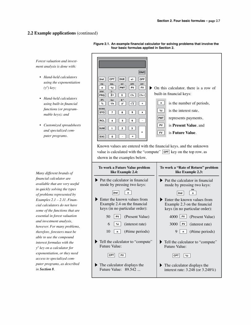
Figure 2.1. An example financial calculator for solving problems that involve the four basic formulas applied in Section 2.
On this calculator, there is a row of built-in financial keys:
n
%i
PMT
PV
FV
is the number of periods,
is the interest rate,
represents payments,
is Present Value, and
is Future Value.
Known values are entered with the financial keys, and the unknown value is calculated with the “compute” key on the top row, as shown in the examples below.
To work a Future Value problemlike Example 2.4:
Put the calculator in financial mode by pressing two keys:
2nd nFIN
Enter the known values fromExample 2.4 on the financial keys (in no particular order):
50 (Present Value)
6 (interest rate)
10 (#time periods)
PV
n
%i
Tell the calculator to “compute”Future Value:
The calculator displays the Future Value: 89.542 ...
CPT FV
To work a “Rate of Return” problemlike Example 2.3:
Put the calculator in financial mode by pressing two keys:
2nd nFIN
Enter the known values fromExample 2.3 on the financial keys (in no particular order):
4000 (Present Value)
3000 (interest rate)
9 (#time periods)
FV
n
PV
Tell the calculator to “compute”Future Value:
The calculator displays the interest rate: 3.248 (or 3.248%)
CPT %i
CPT
Forest valuation and invest-ment analysis is done with:
• Hand-held calculators using the exponentiation (yx) key;
• Hand-held calculators using built-in financial functions (or program-mable keys); and
• Customized spreadsheets and specialized com-puter programs.
Many different brands of financial calculator are available that are very useful in quickly solving the types of problems represented by Examples 2.1 – 2.11. Finan-cial calculators do not have some of the functions that are essential in forest valuation and investment analysis, however. For many problems, therefore, foresters must be able to use the compound interest formulas with the yx key on a calculator for exponentiation, or they need access to specialized com-puter programs, as described in Section 8.
Section 2. Four basic formulas – page 2.8
2.2 Example applications (continued)
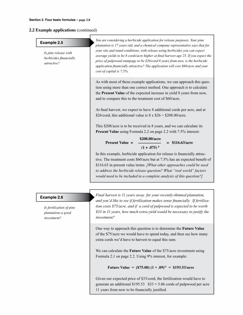
Is pine release withherbicides financiallyattractive?
You are considering a herbicide application for release purposes. Your pine plantation is 17 years old, and a chemical company representative says that for your site and stand conditions, with release using herbicides you can expect average yields to be 8 cords/acre higher at final harvest age 25. If you expect the price of pulpwood stumpage to be $26/cord 8 years from now, is the herbicide application financially attractive? The application will cost $60/acre and your cost of capital is 7.5%.
As with most of these example applications, we can approach this ques-tion using more than one correct method. One approach is to calculate the Present Value of the expected increase in yield 8 years from now, and to compare this to the treatment cost of $60/acre.
At final harvest, we expect to have 8 additional cords per acre, and at $26/cord, this additional value is 8 x $26 = $208.00/acre.
This $208/acre is to be received in 8 years, and we can calculate its Present Value using Formula 2.2 on page 2.2 with 7.5% interest:
In this example, herbicide application for release is financially attrac-tive. The treatment costs $60/acre but at 7.5% has an expected benefit of $116.63 in present value terms. [What other approaches could be used to address the herbicide release question? What “real world” factors would need to be included in a complete analysis of this question?]
Example 2.5
Present Value = = $116.63/acre$208.00/acre
(1 + .075) 8
Is fertilization of pineplantations a goodinvestment?
Final harvest is 11 years away for your recently-thinned plantation, and you’d like to see if fertilization makes sense financially. If fertiliza-tion costs $75/acre, and if a cord of pulpwood is expected to be worth $33 in 11 years, how much extra yield would be necessary to justify the investment?
One way to approach this question is to determine the Future Value of the $75/acre we would have to spend today, and then see how many extra cords we’d have to harvest to equal this sum.
We can calculate the Future Value of the $75/acre investment using Formula 2.1 on page 2.2. Using 9% interest, for example:
Future Value = ($75.00) (1 + .09)11 = $193.53/acre
Given our expected price of $33/cord, the fertilization would have to generate an additional $195.53 $33 = 5.86 cords of pulpwood per acre 11 years from now to be financially justified.
Example 2.6
Section 2. Four basic formulas – page 2.9
2.2 Example applications (continued)Once again, note that some important factors aren’t discussed in these exam-ple applications. We haven’t said, for example, if inflation was included in the prices and the interest rates used in Examples 2.4–2.6, and we aren’t including taxes, risk, and some other factors that may be very important in a complete analysis of whether specific silvicultural practices are financially justified.
Also, in the previous three Examples what impact would it have on our analysis results and investment decisions if we increased the interest rate? In other cases, what if you aren’t very sure of the yield increases for various practices? What if you’re projecting far into the future with highly uncertain stumpage prices? “What if” questions often arise in forest valuation and investment analysis because there are variables and factors we can’t predict with certainty. Assump-tions are necessary, and foresters often evaluate how sensitive their analysis results and investment recommendations are to changes in assumptions like future prices and yields. This process, called “sensitivity analysis,” is discussed in Section 5.4 Risk and uncertainty.
“Real world” analyses may involve taxes, inflation, and other factors not included in these Examples, but dis-cussed in later Sections.
Because prices, yields and other variables can’t be predicted with certainty, assumptions are necessary. “Sensitivity analysis” is discussed in Section 5.4 as a systematic means of dealing with uncertainty in forestry investment analysis.
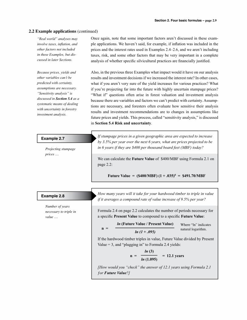
Projecting stumpageprices …
If stumpage prices in a given geographic area are expected to increase by 3.5% per year over the next 6 years, what are prices projected to be in 6 years if they are $400 per thousand board feet (MBF) today?
We can calculate the Future Value of $400/MBF using Formula 2.1 on page 2.2:
Future Value = ($400/MBF) (1 + .035)6 = $491.70/MBF
Example 2.7
Number of yearsnecessary to triple invalue …
How many years will it take for your hardwood timber to triple in value if it averages a compound rate of value increase of 9.5% per year?
Formula 2.4 on page 2.2 calculates the number of periods necessary for a specific Present Value to compound to a specific Future Value:
If the hardwood timber triples in value, Future Value divided by Present Value = 3, and “plugging in” to Formula 2.4 yields:
[How would you “check” the answer of 12.1 years using Formula 2.1 ƒor Future Value?]
Example 2.8
n = = 12.1 years ln (3)
ln (1.095)
n = ln (Future Value / Present Value)
ln (1 + .095)
Where “ln” indicatesnatural logarithm.
Section 2. Four basic formulas – page 2.10
2.2 Example applications (continued)
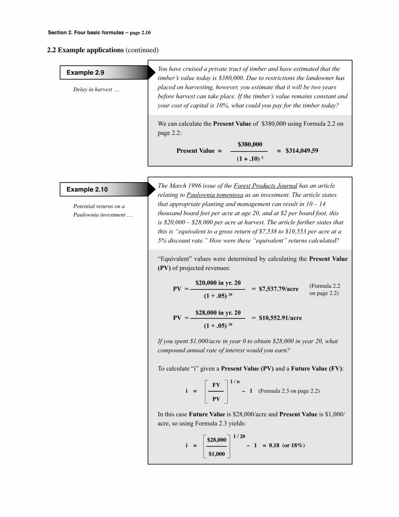
Delay in harvest …
You have cruised a private tract of timber and have estimated that the timber’s value today is $380,000. Due to restrictions the landowner has placed on harvesting, however, you estimate that it will be two years before harvest can take place. If the timber’s value remains constant and your cost of capital is 10%, what could you pay for the timber today?
We can calculate the Present Value of $380,000 using Formula 2.2 on page 2.2:
Example 2.9
Present Value = = $314,049.59$380,000
(1 + .10) 2
Potential returns on aPaulownia investment …
The March 1996 issue of the Forest Products Journal has an article relating to Paulownia tomentosa as an investment. The article states that appropriate planting and management can result in 10 – 14 thousand board feet per acre at age 20, and at $2 per board foot, this is $20,000 – $28,000 per acre at harvest. The article further states that this is “equivalent to a gross return of $7,538 to $10,553 per acre at a 5% discount rate.” How were these “equivalent” returns calculated?
“Equivalent” values were determined by calculating the Present Value (PV) of projected revenues:
If you spent $1,000/acre in year 0 to obtain $28,000 in year 20, what compound annual rate of interest would you earn?
To calculate “i” given a Present Value (PV) and a Future Value (FV):
In this case Future Value is $28,000/acre and Present Value is $1,000/acre, so using Formula 2.3 yields:
Example 2.10
PV = = $7,537.79/acre$20,000 in yr. 20
(1 + .05) 20
(Formula 2.2 on page 2.2)
PV = = $10,552.91/acre$28,000 in yr. 20
(1 + .05) 20
i = – 1 (Formula 2.3 on page 2.2) FV
PV
1 / n
i = – 1 = 0.18 (or 18%)$28,000
$1,000
1 / 20
Section 2. Four basic formulas – page 2.11
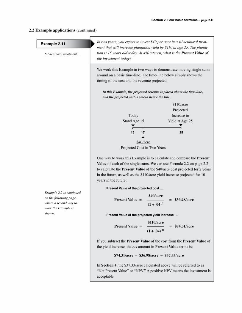
In two years, you expect to invest $40 per acre in a silvicultural treat-ment that will increase plantation yield by $110 at age 25. The planta-tion is 15 years old today. At 4% interest, what is the Present Value of the investment today?
We work this Example in two ways to demonstrate moving single sums around on a basic time-line. The time-line below simply shows the timing of the cost and the revenue projected.
One way to work this Example is to calculate and compare the Present Value of each of the single sums. We can use Formula 2.2 on page 2.2 to calculate the Present Value of the $40/acre cost projected for 2 years in the future, as well as the $110/acre yield increase projected for 10 years in the future:
If you subtract the Present Value of the cost from the Present Value of the yield increase, the net amount in Present Value terms is:
$74.31/acre – $36.98/acre = $37.33/acre
In Section 4, the $37.33/acre calculated above will be referred to as “Net Present Value” or “NPV.” A positive NPV means the investment is acceptable.
2.2 Example applications (continued)
Silvicultural treatment …
Example 2.11
TodayStand Age 15
15 17 25
$40/acreProjected Cost in Two Years
$110/acreProjected
Increase inYield at Age 25
In this Example, the projected revenue is placed above the time-line,and the projected cost is placed below the line.
Present Value = = $36.98/acre$40/acre
(1 + .04) 2
Present Value of the projected cost …
Present Value = = $74.31/acre$110/acre
(1 + .04) 10
Present Value of the projected yield increase …
Example 2.2 is continued on the following page, where a second way to work the Example is shown.
Section 2. Four basic formulas – page 2.12
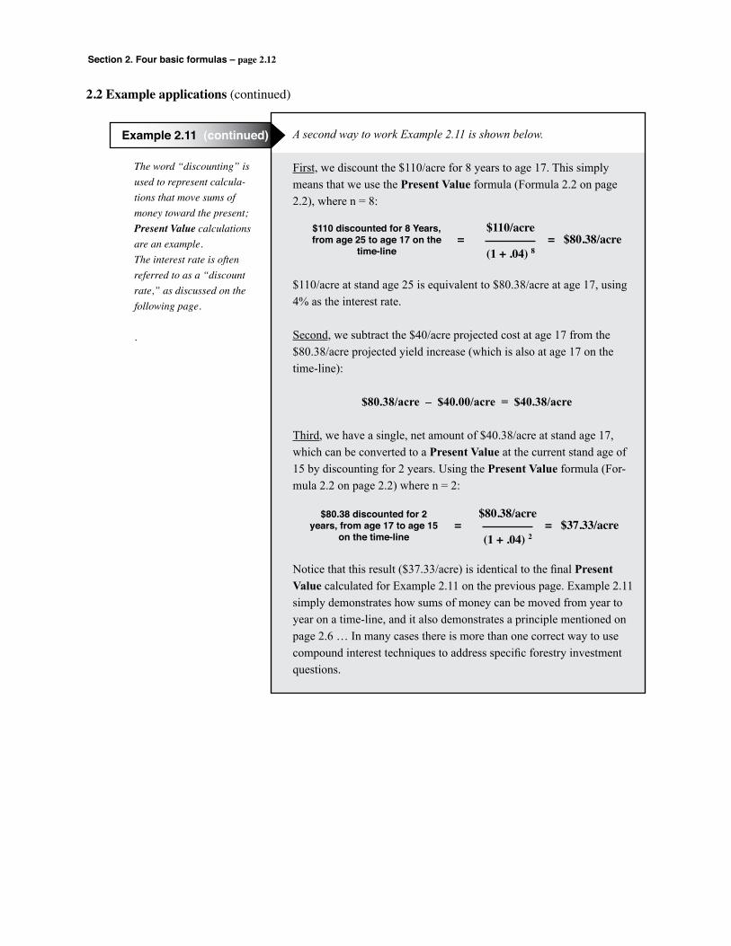
A second way to work Example 2.11 is shown below.
First, we discount the $110/acre for 8 years to age 17. This simply means that we use the Present Value formula (Formula 2.2 on page 2.2), where n = 8:
$110/acre at stand age 25 is equivalent to $80.38/acre at age 17, using 4% as the interest rate.
Second, we subtract the $40/acre projected cost at age 17 from the $80.38/acre projected yield increase (which is also at age 17 on the time-line):
$80.38/acre – $40.00/acre = $40.38/acre
Third, we have a single, net amount of $40.38/acre at stand age 17, which can be converted to a Present Value at the current stand age of 15 by discounting for 2 years. Using the Present Value formula (For-mula 2.2 on page 2.2) where n = 2:
Notice that this result ($37.33/acre) is identical to the final Present Value calculated for Example 2.11 on the previous page. Example 2.11 simply demonstrates how sums of money can be moved from year to year on a time-line, and it also demonstrates a principle mentioned on page 2.6 … In many cases there is more than one correct way to use compound interest techniques to address specific forestry investment questions.
2.2 Example applications (continued)
The word “discounting” is used to represent calcula-tions that move sums of money toward the present; Present Value calculations are an example.The interest rate is often referred to as a “discount rate,” as discussed on the following page.
.
Example 2.11 (continued)
= = $80.38/acre$110/acre
(1 + .04) 8
$110 discounted for 8 Years, from age 25 to age 17 on the
time-line
= = $37.33/acre$80.38/acre
(1 + .04) 2
$80.38 discounted for 2 years, from age 17 to age 15
on the time-line

Section 2. Four basic formulas – page 2.13
Formulas 2.1–2.4 were referred to as “Four Basic Formulas” in Section 2.1. They are very useful for some types of forestry investment questions. There are other formulas, however, that are also used in calculating “net present value,” “benefit/cost ratios,” and other financial criteria. These formulas are the subject of Section 3, where they are developed and applied to example forestry problems.
Before proceeding, however, several terms and concepts that are basic to using the formulas should be summarized:
v Compounding and discountingWhen the general formula for compound interest is used to calculate a Future Value, a Present Value is multiplied by (1+i)n – an example of compounding. To “compound” a number is therefore to calculate a Future Value with com-pound interest using the basic formula (2.1 on page 2.2), or using other formu-las for Future Value. “Discounting,” meanwhile, is the reciprocal operation. To divide a number by (1+i)n is an example, and to calculate a Present Value is therefore often referred to as “discounting.” If the interest rate is positive, of course, numbers get larger and larger when they are compounded for longer periods of time, and they get successively smaller when discounted for longer periods.
v EquivalenceAs discussed in Section 1, money has a time value, and a dollar received today is not equivalent to a dollar to be received in the future. Compound interest formulas are used, however, to calculate sums of money that can be termed “equivalent” in different time periods. In Example 2.10, $20,000/acre in year 20 and $7,537.79 today were shown to be “equivalent” at 5% interest. In gen-eral, equivalent present and future values are determined by compounding and discounting for a specific time with a specific rate of compound interest.
v The interest rateIn some of the example applications in Section 2.2, we referred to the rate of compound interest using terms like “cost of capital.” The compound interest rate is also sometimes referred to as the “guiding rate,” the “hurdle rate,” and the “alternative rate of return,” and since the interest rate is used in discount-ing it’s sometimes referred to simply as the “discount rate.” These terms will be used in some of the examples and problems in later Sections of the work-book. Terms and concepts associated with the compound rate of interest are explained in detail in Section 5.6 Choosing a discount rate.
2.3 Basic terms and concepts
Terms and concepts: • Compounding and discounting • Equivalence • The interest rate • Cash-flow diagrams • End-of-year assumption
Compounding and discounting are math-ematical operations using compound interest formulas.
Compounding and discounting are used to determine sums of money that are “equivalent” over time.
The interest rate has several names in forestry investment analysis. These and other concepts are explained in Section 5.
Section 2. Four basic formulas – page 2.14
2.3. Basic terms and concepts (continued)
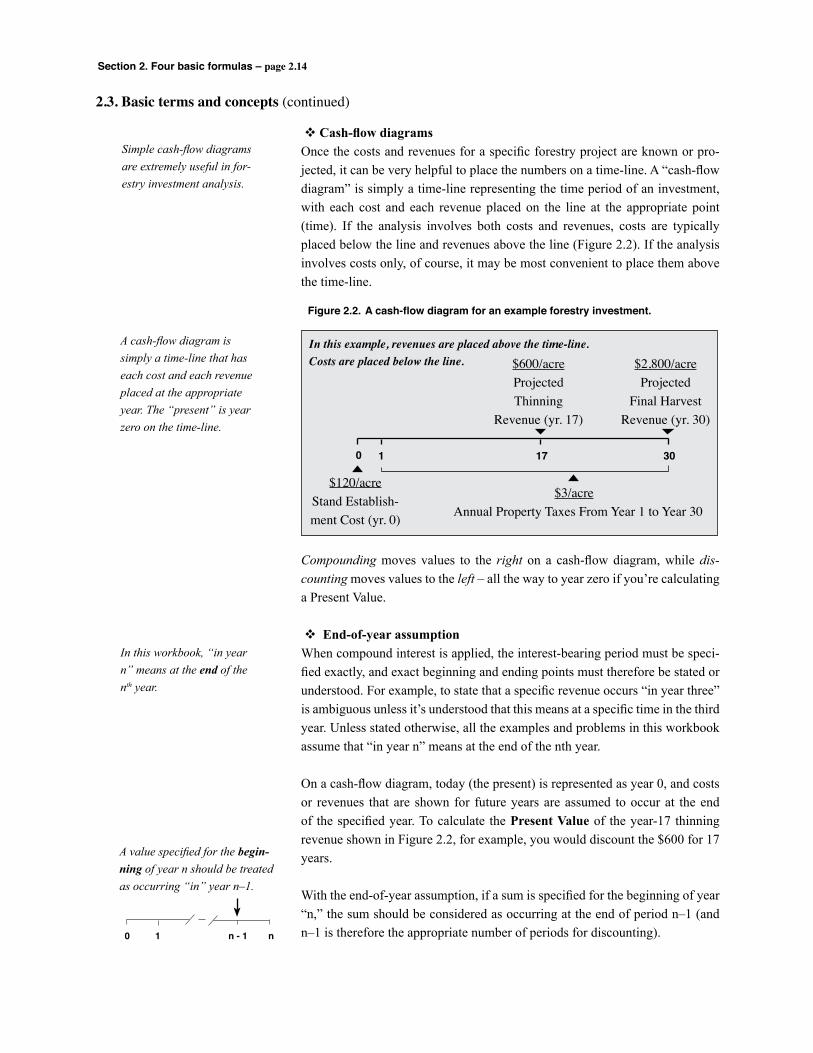
v Cash-flow diagramsOnce the costs and revenues for a specific forestry project are known or pro-jected, it can be very helpful to place the numbers on a time-line. A “cash-flow diagram” is simply a time-line representing the time period of an investment, with each cost and each revenue placed on the line at the appropriate point (time). If the analysis involves both costs and revenues, costs are typically placed below the line and revenues above the line (Figure 2.2). If the analysis involves costs only, of course, it may be most convenient to place them above the time-line.
A cash-flow diagram is simply a time-line that has each cost and each revenue placed at the appropriate year. The “present” is year zero on the time-line.
Figure 2.2. A cash-flow diagram for an example forestry investment.
$120/acreStand Establish-ment Cost (yr. 0)
0 1 17 30
$600/acreProjectedThinning
Revenue (yr. 17)
$2,800/acreProjected
Final HarvestRevenue (yr. 30)
$3/acreAnnual Property Taxes From Year 1 to Year 30
In this example, revenues are placed above the time-line.Costs are placed below the line.
Compounding moves values to the right on a cash-flow diagram, while dis-counting moves values to the left – all the way to year zero if you’re calculating a Present Value.
v End-of-year assumptionWhen compound interest is applied, the interest-bearing period must be speci-fied exactly, and exact beginning and ending points must therefore be stated or understood. For example, to state that a specific revenue occurs “in year three” is ambiguous unless it’s understood that this means at a specific time in the third year. Unless stated otherwise, all the examples and problems in this workbook assume that “in year n” means at the end of the nth year.
On a cash-flow diagram, today (the present) is represented as year 0, and costs or revenues that are shown for future years are assumed to occur at the end of the specified year. To calculate the Present Value of the year-17 thinning revenue shown in Figure 2.2, for example, you would discount the $600 for 17 years.
With the end-of-year assumption, if a sum is specified for the beginning of year “n,” the sum should be considered as occurring at the end of period n–1 (and n–1 is therefore the appropriate number of periods for discounting).
Simple cash-flow diagrams are extremely useful in for-estry investment analysis.
In this workbook, “in year n” means at the end of the nth year.
A value specified for the begin-ning of year n should be treated as occurring “in” year n–1.
0 1 n - 1 n
Section 2. Four basic formulas – page 2.15
Section 2. Four basic formulas
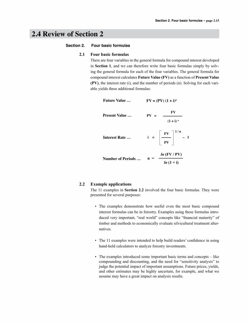
2.1 Four basic formulas There are four variables in the general formula for compound interest developed
in Section 1, and we can therefore write four basic formulas simply by solv-ing the general formula for each of the four variables. The general formula for compound interest calculates Future Value (FV) as a function of Present Value (PV), the interest rate (i), and the number of periods (n). Solving for each vari-able yields three additional formulas:
2.2 Example applications The 11 examples in Section 2.2 involved the four basic formulas. They were
presented for several purposes:
• The examples demonstrate how useful even the most basic compound interest formulas can be in forestry. Examples using these formulas intro-duced very important, “real world” concepts like “financial maturity” of timber and methods to economically evaluate silvicultural treatment alter-natives.
• The 11 examples were intended to help build readers’ confidence in using hand-held calculators to analyze forestry investments.
• The examples introduced some important basic terms and concepts – like compounding and discounting, and the need for “sensitivity analysis” to judge the potential impact of important assumptions. Future prices, yields, and other estimates may be highly uncertain, for example, and what we assume may have a great impact on analysis results.
2.4 Review of Section 2
FV = (PV) (1 + i)n
PV = FV
(1 + i) n
i = – 1 FV
PV
1 / n
n = ln (FV / PV)
ln (1 + i)
Future Value …
Present Value …
Interest Rate …
Number of Periods …

Section 2. Four basic formulas – page 2.16
2.4. Review of Section 2 (continued)
• Finally, the examples showed that there can be more than one correct way to address forest valuation and investment analysis questions. To evalu-ate a silvicultural treatment alternative, for example, we may estimate the Present Value of a projected income or the Future Value of a specific cost, but in either case we use compound interest formulas to account for the time value of the money involved. We then compare Future Values to Future Values, Present Values to Present Values, or the interest rate earned to rates that can be earned in other investments of comparable duration, risk, and liquidity.
2.3 Basic terms and concepts Several terms and concepts were summarized before developing and using the
full set of compound interest formulas in Section 3:
• When using compound interest formulas to calculate a specific Future Value we’re “compounding” a number. We’re “discounting” when we calculate a Present Value.
• By using compound interest formulas appropriately, “equivalent” Pres-ent and Future Values are determined for a specific time period and a specific interest rate.
• The interest rate may be called the “cost of capital,” the “guiding rate,” “hurdle rate,” the “alternative rate of return,” or simply the “discount rate.” These terms are used in the examples and problems in Sections 3 and 4, and are explained with other interest rate concepts in Section 5.6 Choosing a discount rate.
• Cash-flow diagrams are extremely useful in forest valuation and invest-ment analysis. The first step in most investment analysis situations should be to draw a cash-flow diagram by placing all costs and revenues on a time-line.
• In this workbook, “in year n” means at the end of the nth year. This end-of-year assumption provides consistency for developing and using compound interest formulas and techniques.
Section 3. Twelve formulas – page 3.1
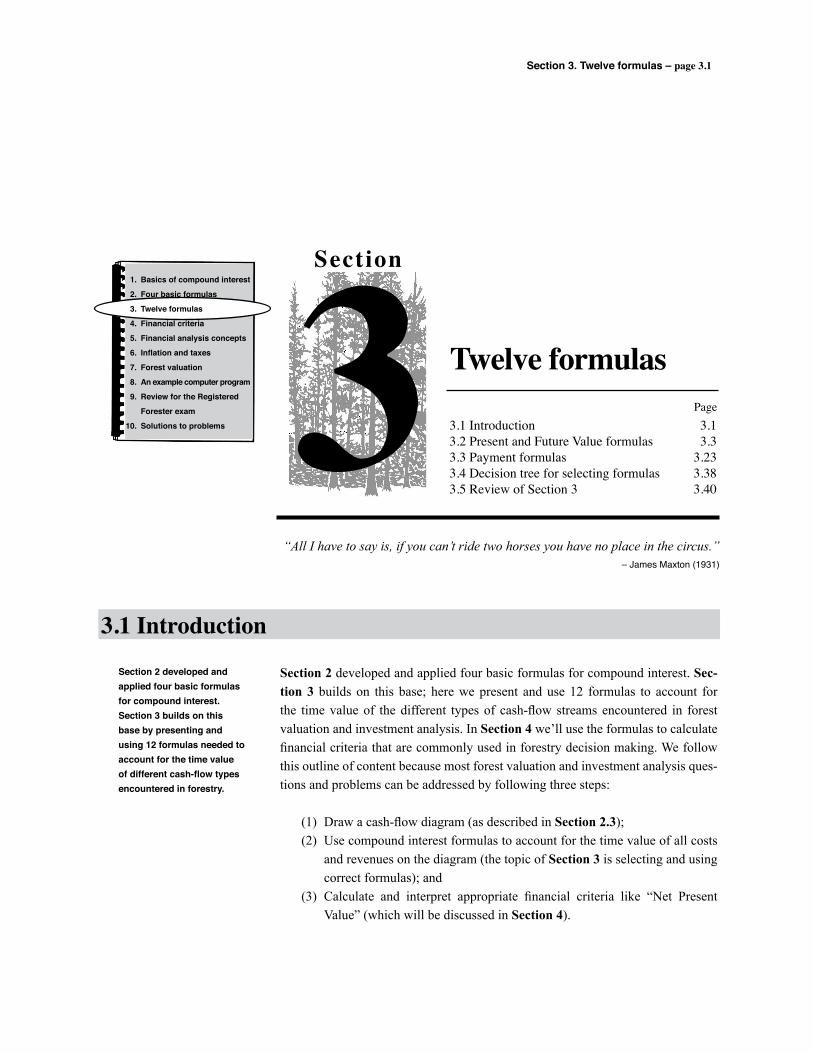
Section
3 Twelve formulas
3.1 Introduction 3.13.2 Present and Future Value formulas 3.33.3 Payment formulas 3.233.4 Decision tree for selecting formulas 3.383.5 Review of Section 3 3.40
“All I have to say is, if you can’t ride two horses you have no place in the circus.”– James Maxton (1931)
Section 2 developed and applied four basic formulas for compound interest. Sec-tion 3 builds on this base; here we present and use 12 formulas to account for the time value of the different types of cash-flow streams encountered in forest valuation and investment analysis. In Section 4 we’ll use the formulas to calculate financial criteria that are commonly used in forestry decision making. We follow this outline of content because most forest valuation and investment analysis ques-tions and problems can be addressed by following three steps:
(1) Draw a cash-flow diagram (as described in Section 2.3); (2) Use compound interest formulas to account for the time value of all costs
and revenues on the diagram (the topic of Section 3 is selecting and using correct formulas); and
(3) Calculate and interpret appropriate financial criteria like “Net Present Value” (which will be discussed in Section 4).
3.1 Introduction
Page
Section 2 developed and applied four basic formulas for compound interest. Section 3 builds on this base by presenting and using 12 formulas needed to account for the time value of different cash-flow types encountered in forestry.
1. Basics of compound interest
2. Four basic formulas
3. Twelve formulas
4. Financial criteria
5. Financial analysis concepts
6. Inflation and taxes
7. Forest valuation
8. An example computer program
9. Review for the Registered
Forester exam
10. Solutions to problems

Section 3. Twelve formulas – page 3.2
3.1 Introduction (continued)
The overall pattern we use for decision tree development follows a diagram presented by J.E. Gunter and H.L. Haney, 1978, “A Decision Tree for Compound Interest Formulas,” South. J. Appl. For. 2(3):107.
In Section 3 we develop a “decision tree” diagram for selecting among 12 compound interest formulas. The diagram is actually a composite of three diagrams, however, based on what you’re calculating …
Present Valueor
Future Value
Payments
To calculate …
Interest Rate orNumber of Periods
Present Value and Future Value Formulas
Six Present and Future Valueformulas are developed and applied
in Section 3.2
12 Formulas in 3 Groups
Payment Formulas
Four payment formulas are developedand applied in Section 3.3
Formulas for “i” and “n”
Two formulas developed and appliedin Section 2 are included in the
12-formula decision tree diagramin Section 3.4
In Section 3 we present exam-ples for each formula discussed. We also provide problems, how-ever, and we strongly encourage readers to “put their pencils to paper.” Solutions to all prob-lems are in Section 10.
In Section 3.2 we develop and apply six formulas for Present and Future Value, and in Section 3.3 we develop and apply four formulas for payments. Each of these formula “groups” is developed and presented using a decision tree diagram for formula selection. In Section 3.4 we present a complete diagram for compound interest formulas that includes these two groups of formulas, plus a third group comprised of two formulas that were developed and applied in Section 2.

Section 3. Twelve formulas – page 3.3
In Section 1 we developed the basic, general formula for compound interest. We called this the “Future Value” formula since it calculates a Future Value that’s equivalent to a specific Present Value for a given interest rate and time period:
Future Value = (Present Value) (1 + i)n
Since Present Value occurs in year 0 and Future Value in year n, standard notation is Vn for Future Value and Vo for Present Value. Since Vn and Vo each represent a single sum of money, the formula is referred to as the Future Value of a Single Sum:
3.2 Present and Future Value formulas
In this part of Section 3 we develop a decision tree dia-gram with six Present Value and Future Value formulas. The first two formulas were devel-oped and applied in Sections 1 and 2.
Formula 3.1 – Future Value of a Single Sum Vn = V0 (1 + i)n
On a time-line, we represent Vn and Vo as two single sums – one occurs at the end of year n and one occurs in year 0 (Figure 3.1).
Figure 3.1. Cash-flow diagram for the Future Value of a Single Sum.
0 n
V0 Vn
The Future Value of a Single Sum formula compounds a single Present Value for “n” years.
In Section 2 we developed three more formulas by solving the formula above for each of the other three variables. In addition to Future Value, we pre-sented and applied formulas for Present Value (Vo), the interest rate (i), and the number of time periods (n). The Present Value formula developed and used in Section 2 is simply the reciprocal of the Future Value formula above. It’s more appropriately termed the Present Value of a Single Sum formula:
Formula 3.2 – Present Value of a Single Sum V0 = Vn
(1 + i)n

Section 3. Twelve formulas – page 3.4
3.2 Present and Future Value Formulas (continued)
Formula 3.2 is used to discount a single future sum to the present, as shown in Figure 3.2.
Figure 3.2. Cash-flow diagram for the Present Value of a Single Sum.
Formulas 3.1 and 3.2 are single sum formulas because they compound or discount one cost or revenue at a time.
0 n
V0 Vn
The Present Value of a Single Sum formula discounts a single Future Value for “n” years.
Formula 3.1 is used to compound and formula 3.2 is used to discount single-sum revenues like thinning or final harvest income, and single-sum costs like fertilization or other silvicultural practices. This was demonstrated in the exam-ples that applied the Present and Future Value formulas in Section 2.
What if your forestry investment includes an income or an expense that occurs every year or every “n” years? Our cash-flow diagram may include a hunting lease income that occurs each year, for example, or it may include annual prop-erty taxes as a cost of timberland ownership. These are series of uniform costs and revenues. Examples of uniform annual and periodic costs and revenues are numerous in forestry, but only four formulas are needed to calculate present and future value for the different types of series.
Many forestry investments include series of costs and revenues that are uniform. With four formulas for cash flow series, foresters can account for their time-value.
Vn = V0 (1 + i)n
V0 = Vn
(1 + i) n
Future Value of a Single Sum
Present Value of a Single Sum
Future Valueof a TerminatingAnnual Series
Vn = a(1 + i)n – 1
i 0 1a
Present Valueof a TerminatingAnnual Series
V0 = a(1 + i)n – 1
i (1 + i)n
V0
0 1a
V0 = ai
Present Value of aPerpetual Annual Series
V0
0 1a
Present and Future Value Formulas
3.1
V0 = Vn
(1 + i) n – 1Present Value of a Perpetual Periodic Series
V0
0 na
Future Value
Present Value
Future Value
Present Value
Present Value
Present Value
Series
Single-sum
Present Valueor
Future Value
Formulas 3.1 and 3.2 (above) apply to single sums like one-time timber sale revenues or fertilization costs.
To complete the decision tree diagram, next we develop four formulas (3.3–3.6) that cal-culate Present Value or Future Value for uniform series of annual or periodic costs and revenues.
3.2
3.3
3.4
3.5
3.6
Formula selection can be represented by a decision tree diagram:
In selecting a Present Value formula or a Future Value formula, we must first choose between formulas that apply to single-sum costs and revenues, and formulas for costs and revenues that are part of a uniform series.
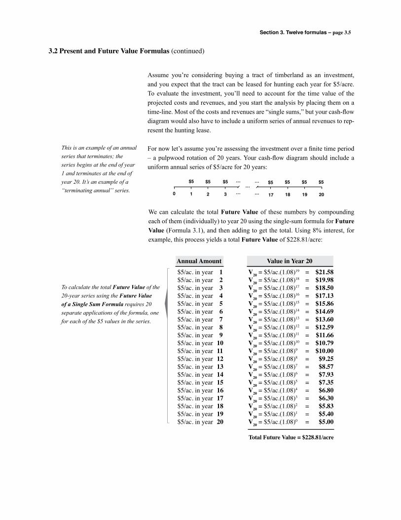
Section 3. Twelve formulas – page 3.5
Assume you’re considering buying a tract of timberland as an investment, and you expect that the tract can be leased for hunting each year for $5/acre. To evaluate the investment, you’ll need to account for the time value of the projected costs and revenues, and you start the analysis by placing them on a time-line. Most of the costs and revenues are “single sums,” but your cash-flow diagram would also have to include a uniform series of annual revenues to rep-resent the hunting lease.
For now let’s assume you’re assessing the investment over a finite time period – a pulpwood rotation of 20 years. Your cash-flow diagram should include a uniform annual series of $5/acre for 20 years:
This is an example of an annual series that terminates; the series begins at the end of year 1 and terminates at the end of year 20. It’s an example of a “terminating annual” series.
To calculate the total Future Value of the 20-year series using the Future Value of a Single Sum Formula requires 20 separate applications of the formula, one for each of the $5 values in the series.
3.2 Present and Future Value Formulas (continued)
0 1 2 3 ……
…
……
18 19 2017
$5 $5 $5 $5 $5 $5$5
We can calculate the total Future Value of these numbers by compounding each of them (individually) to year 20 using the single-sum formula for Future Value (Formula 3.1), and then adding to get the total. Using 8% interest, for example, this process yields a total Future Value of $228.81/acre:
$5/ac. in year 1 V20 = $5/ac.(1.08)19 = $21.58$5/ac. in year 2 V20 = $5/ac.(1.08)18 = $19.98$5/ac. in year 3 V20 = $5/ac.(1.08)17 = $18.50$5/ac. in year 4 V20 = $5/ac.(1.08)16 = $17.13$5/ac. in year 5 V20 = $5/ac.(1.08)15 = $15.86$5/ac. in year 6 V20 = $5/ac.(1.08)14 = $14.69$5/ac. in year 7 V20 = $5/ac.(1.08)13 = $13.60$5/ac. in year 8 V20 = $5/ac.(1.08)12 = $12.59$5/ac. in year 9 V20 = $5/ac.(1.08)11 = $11.66$5/ac. in year 10 V20 = $5/ac.(1.08)10 = $10.79$5/ac. in year 11 V20 = $5/ac.(1.08)9 = $10.00$5/ac. in year 12 V20 = $5/ac.(1.08)8 = $9.25$5/ac. in year 13 V20 = $5/ac.(1.08)7 = $8.57$5/ac. in year 14 V20 = $5/ac.(1.08)6 = $7.93$5/ac. in year 15 V20 = $5/ac.(1.08)5 = $7.35$5/ac. in year 16 V20 = $5/ac.(1.08)4 = $6.80$5/ac. in year 17 V20 = $5/ac.(1.08)3 = $6.30$5/ac. in year 18 V20 = $5/ac.(1.08)2 = $5.83$5/ac. in year 19 V20 = $5/ac.(1.08)1 = $5.40$5/ac. in year 20 V20 = $5/ac.(1.08)0 = $5.00
Annual Amount Value in Year 20
Total Future Value = $228.81/acre
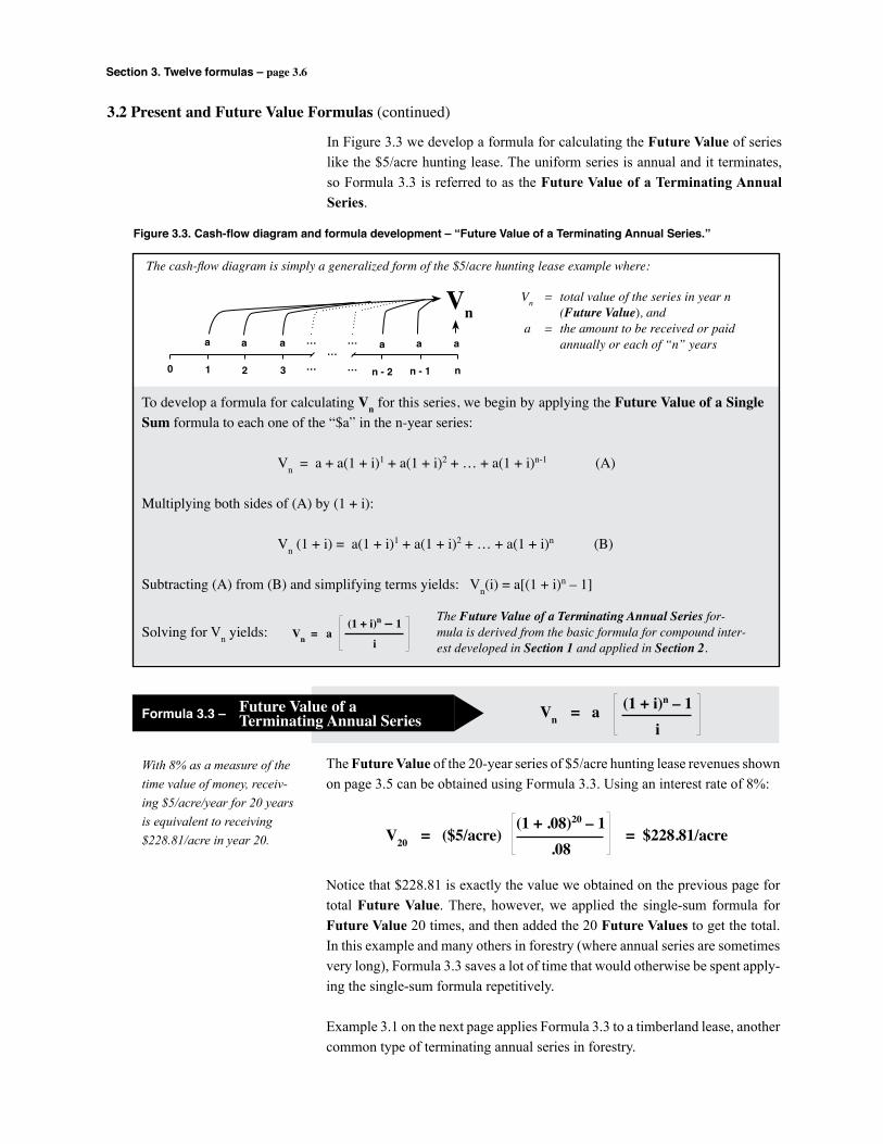
Section 3. Twelve formulas – page 3.6
In Figure 3.3 we develop a formula for calculating the Future Value of series like the $5/acre hunting lease. The uniform series is annual and it terminates, so Formula 3.3 is referred to as the Future Value of a Terminating Annual Series.
With 8% as a measure of the time value of money, receiv-ing $5/acre/year for 20 years is equivalent to receiving $228.81/acre in year 20.
3.2 Present and Future Value Formulas (continued)
0 1 2 3 ……
…
……
n - 1 nn - 2
a a a a aa
Vn
Figure 3.3. Cash-flow diagram and formula development – “Future Value of a Terminating Annual Series.”
The cash-flow diagram is simply a generalized form of the $5/acre hunting lease example where:
Vn = total value of the series in year n (Future Value), and a = the amount to be received or paid annually or each of “n” years
To develop a formula for calculating Vn for this series, we begin by applying the Future Value of a Single Sum formula to each one of the “$a” in the n-year series:
Vn = a + a(1 + i)1 + a(1 + i)2 + … + a(1 + i)n-1 (A)
Multiplying both sides of (A) by (1 + i):
Vn (1 + i) = a(1 + i)1 + a(1 + i)2 + … + a(1 + i)n (B)
Subtracting (A) from (B) and simplifying terms yields: Vn(i) = a[(1 + i)n – 1]
Solving for Vn yields: Vn = a(1 + i)n – 1
i
The Future Value of a Terminating Annual Series for-mula is derived from the basic formula for compound inter-est developed in Section 1 and applied in Section 2.
Formula 3.3 – V0 = Future Value of aTerminating Annual Series Vn = a (1 + i)n – 1
i
The Future Value of the 20-year series of $5/acre hunting lease revenues shown on page 3.5 can be obtained using Formula 3.3. Using an interest rate of 8%:
Notice that $228.81 is exactly the value we obtained on the previous page for total Future Value. There, however, we applied the single-sum formula for Future Value 20 times, and then added the 20 Future Values to get the total. In this example and many others in forestry (where annual series are sometimes very long), Formula 3.3 saves a lot of time that would otherwise be spent apply-ing the single-sum formula repetitively.
Example 3.1 on the next page applies Formula 3.3 to a timberland lease, another common type of terminating annual series in forestry.
V20 = ($5/acre)(1 + .08)20 – 1
.08= $228.81/acre
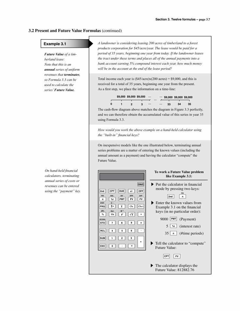
Section 3. Twelve formulas – page 3.7
2nd CPT DUE +/- OFF
n %i PMT PV FV
ON/C
FRQ ∑+ σn
% 1/x yx ÷
σn-1x
√ x
STO 7 8 9 x
4 5 6 _RCL
1 2 3SUM
0 . =EXC
+
FIN BAL INT APR EFF
STAT ∑ –
∆% lnx e x
DECIMAL
To work a Future Value problemlike Example 3.1:
Put the calculator in financial mode by pressing two keys:
2nd nFIN
Enter the known values fromExample 3.1 on the financial keys (in no particular order):
9000 (Payment)
5 (interest rate)
35 (#time periods)
PMT
n
%i
Tell the calculator to “compute”Future Value:
The calculator displays the Future Value: 812882.76
CPT FV
Future Value of a tim-berland lease:Note that this is an annual series of uniform revenues that terminates, so Formula 3.3 can be used to calculate the series’ Future Value.
Example 3.1 A landowner is considering leasing 200 acres of timberland to a forest products corporation for $45/acre/year. The lease would be paid for a period of 35 years, beginning one year from today. If the landowner leases the tract under these terms and places all of the annual payments into a bank account earning 5% compound interest each year, how much money will be in the account at the end of the lease period?
Total income each year is ($45/acre)x(200 acres) = $9,000, and this is received for a total of 35 years, beginning one year from the present. As a first step, we place the information on a time-line:
The cash-flow diagram above matches the diagram in Figure 3.3 perfectly, and we can therefore obtain the accumulated value of this series in year 35 using Formula 3.3.
How would you work the above example on a hand-held calculator using the “built-in” financial keys?
On inexpensive models like the one illustrated below, terminating annual series problems are a matter of entering the known values (including the annual amount as a payment) and having the calculator “compute” the Future Value.
3.2 Present and Future Value Formulas (continued)
0 1 2 3 ……
…
……
34 3533
$9,000 $9,000 $9,000 $9,000 $9,000 $9,000
On hand-held financial calculators, terminating annual series of costs or revenues can be entered using the “payment” key.

Section 3. Twelve formulas – page 3.8
3.2 Present and Future Value Formulas (continued)
The formula for the Present Value of a Terminating Annual Series discounts uniform annual series of costs and/or revenues to the present. The cash flow diagram for the Present Value of a Terminating Annual Series is very similar the one in Figure 3.3 for the Future Value of such series. In fact the cash-flow pattern is identical – a uniform series of “$a” per year that terminates in year n (Figure 3.4). The only difference is that we’re now calculating Present Value instead of Future Value.
Using 8% as a measure of the time value of money, receiv-ing $5/acre/year for 20 years is equivalent to $49.09/acre today.
Figure 3.4. Cash-flow diagram and formula development – “Present Value of a Terminating Annual Series.”
We can develop a formula for this series by using Formula 3.3 for Future Value of the series. That is, we can calculate Present Value for any single-sum Future Value using Formula 3.2 Present Value of a Single Sum. [Once we apply Formula 3.3 to the series, it has been converted into an equivalent single sum in year n.]
The formula for Present Value of a Terminating Annual Series is therefore Formula 3.3, the Future Value formula, divided by (1+i) :
V0 = a(1 + i)n – 1
i(1 + i)n
The Present Value of a Terminating Annual Series formula is obtained by dividing the Future Value formula (3.3) by (1+i)n. We’re simply discounting a Future Value to the present.
Formula 3.4 – V0 = Present Value of aTerminating Annual Series Vn = a (1 + i)n – 1
i(1 + i)n
The Present Value of the $5/acre hunting lease series on page 3.5 can be obtained using Formula 3.4:
If you discounted all 20 of the $5/acre revenues to year 0 at 8% separately, their total Present Value would be $49.09.
V0 = ($5/acre)(1 + .08)20 – 1.08(1 + .08)20
= $49.09/acre
V0 = total value of the series in year n (Present Value) a = the amount to be received or paid annually or each of “n” years0 1 2 3 …
……
……
n - 1 nn - 2
a a a a aa
V0
To calculate the Present Value of the hunting lease on a hand-held calculator using the “built-in” financial keys …
Enter the known values fromExample 3.1 on the financial keys (in no particular order):
5 (Enter the $5 as a Payment)
8 (interest rate)
20 (#time periods)
PMT
n
%i
Tell the calculator to “compute”Present Value:
The calculator displays the Present Value: 49.09
CPT PV
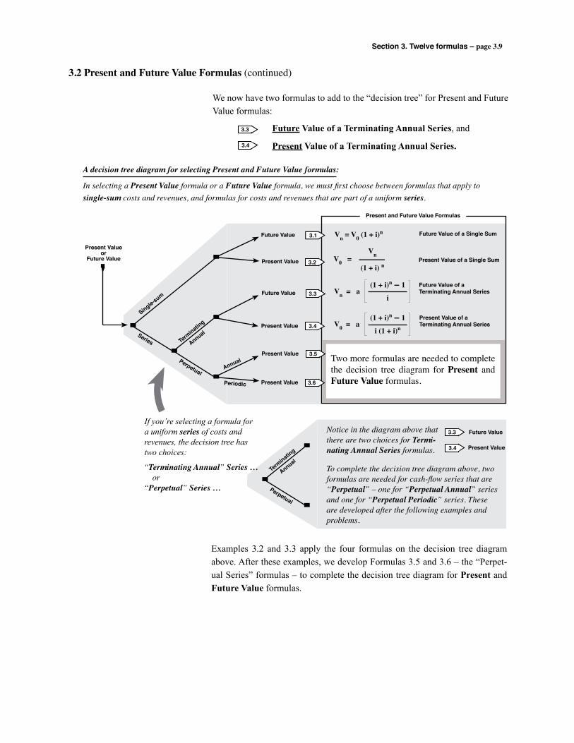
Section 3. Twelve formulas – page 3.9
We now have two formulas to add to the “decision tree” for Present and Future Value formulas:
3.2 Present and Future Value Formulas (continued)
Vn = V0 (1 + i)n
V0 = Vn
(1 + i) n
Future Value of a Single Sum
Present Value of a Single Sum
Future Value of a Terminating Annual SeriesVn = a
(1 + i)n – 1i
Present Value of a Terminating Annual SeriesV0 = a
(1 + i)n – 1i (1 + i)n
V0 = ai
Present Value of aPerpetual Annual Series
V0
0 1a
Present and Future Value Formulas
3.1
V0 = Vn
(1 + i) n – 1Present Value of a Perpetual Periodic Series
V0
0 na
Future Value
Present Value
Future Value
Present Value
Present Value
Present Value
Series
Single-sum
Present Valueor
Future Value
Two more formulas are needed to complete the decision tree diagram for Present and Future Value formulas.
3.2
3.3
3.4
3.5
3.6
3.3
3.4
Future Value of a Terminating Annual Series, and
Present Value of a Terminating Annual Series.
A decision tree diagram for selecting Present and Future Value formulas:
In selecting a Present Value formula or a Future Value formula, we must first choose between formulas that apply to single-sum costs and revenues, and formulas for costs and revenues that are part of a uniform series.
Annual
Periodic
Perpetual
Terminatin
g
Annual
3.3
3.4
Perpetual
Terminatin
g
Annual
Notice in the diagram above that there are two choices for Termi-nating Annual Series formulas.
To complete the decision tree diagram above, two formulas are needed for cash-flow series that are “Perpetual” – one for “Perpetual Annual” series and one for “Perpetual Periodic” series. These are developed after the following examples and problems.
Future Value
Present Value
“Terminating Annual” Series … or“Perpetual” Series …
If you’re selecting a formula for a uniform series of costs and revenues, the decision tree has two choices:
Examples 3.2 and 3.3 apply the four formulas on the decision tree diagram above. After these examples, we develop Formulas 3.5 and 3.6 – the “Perpet-ual Series” formulas – to complete the decision tree diagram for Present and Future Value formulas.
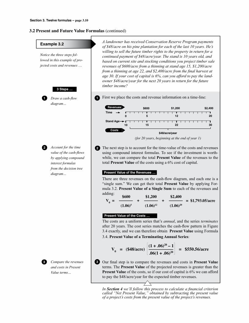
Section 3. Twelve formulas – page 3.10
Notice the three steps fol-lowed in this example of pro-jected costs and revenues …
A landowner has received Conservation Reserve Program payments of $48/acre on his pine plantation for each of the last 10 years. He’s willing to sell the future timber rights to the property in return for a continued payment of $48/acre/year. The stand is 10 years old, and based on current site and stocking conditions you project timber sale revenues of $600/acre from a thinning at stand age 15, $1,200/acre from a thinning at age 22, and $2,400/acre from the final harvest at age 30. If your cost of capital is 6%, can you afford to pay the land-owner $48/acre/year for the next 20 years in return for the future timber income?
First we place the costs and revenue information on a time-line:
The next step is to account for the time-value of the costs and revenues using compound interest formulas. To see if the investment is worth-while, we can compare the total Present Value of the revenues to the total Present Value of the costs using a 6% cost of capital.
There are three revenues on the cash-flow diagram, and each one is a “single sum.” We can get their total Present Value by applying For-mula 3.2. Present Value of a Single Sum to each of the revenues and adding:
The costs are a uniform series that’s annual, and the series terminates after 20 years. The cost series matches the cash-flow pattern in Figure 3.4 exactly, and we can therefore obtain Present Value using Formula 3.4. Present Value of a Terminating Annual Series:
Our final step is to compare the revenues and costs in Present Value terms. The Present Value of the projected revenues is greater than the Present Value of the costs, so if our cost of capital is 6% we can afford to pay the $48/acre/year for the expected timber revenues.
In Section 4 we’ll follow this process to calculate a financial criterion called “Net Present Value,” obtained by subtracting the present value of a project’s costs from the present value of the project’s revenues.
Example 3.2
3.2 Present and Future Value Formulas (continued)
Draw a cash-flow diagram…
Account for the time value of the cash-flows by applying compound interest formulas from the decision tree diagram…
Compare the revenues and costs in Present Value terms…
3 Steps …
1
2
3
1
0 5 12 20
10 15 22 30
Time
Stand Age
Revenues
Costs
$600 $1,200 $2,400
$48/acre/year
(for 20 years, beginning at the end of year 1)
2
Present Value of the Revenues …
V0 = $600
(1.06)5+
$1,200
(1.06)12+
$2,400
(1.06)20= $1,793.05/acre
Present Value of the Costs …
V0 = ($48/acre)(1 + .06)20 – 1.06(1 + .06)20
= $550.56/acre
3
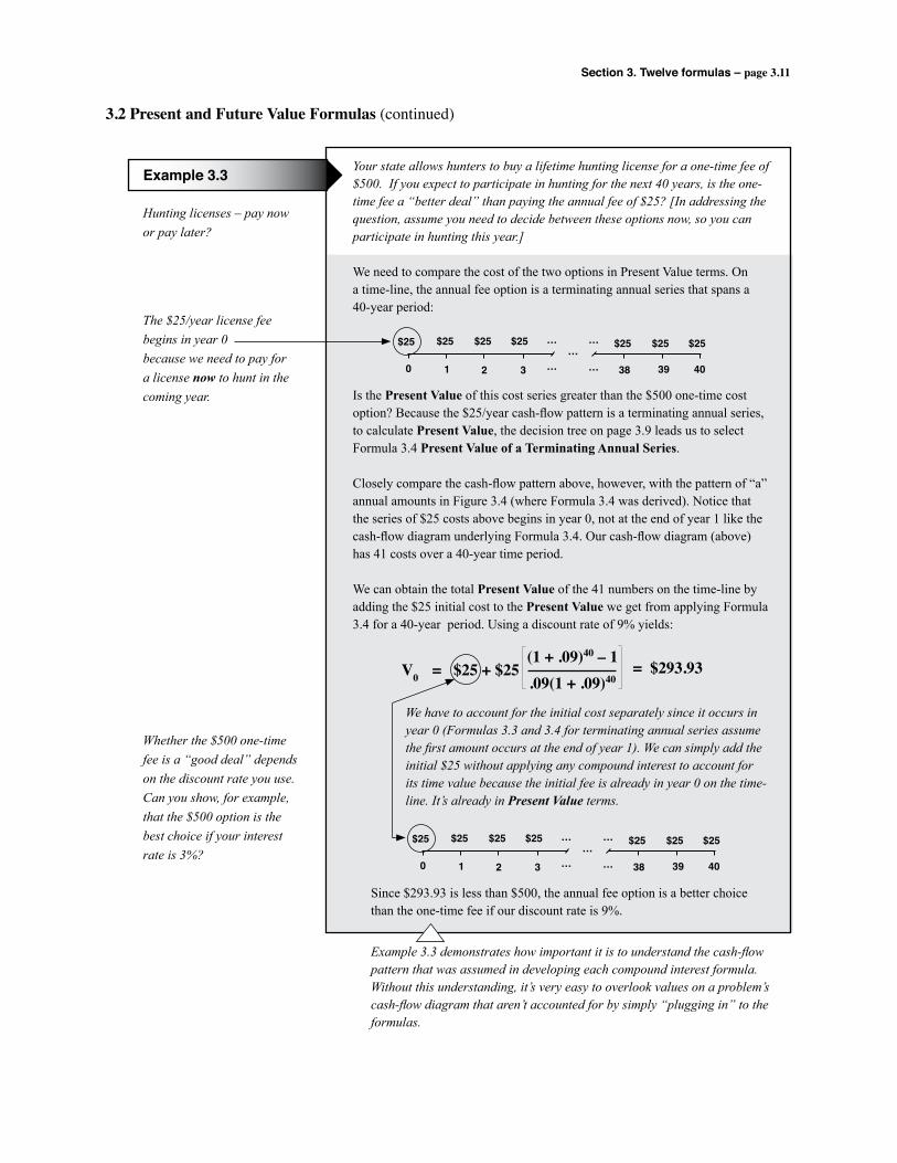
Section 3. Twelve formulas – page 3.11
Hunting licenses – pay now or pay later?
The $25/year license fee begins in year 0 because we need to pay for a license now to hunt in the coming year.
Whether the $500 one-time fee is a “good deal” depends on the discount rate you use. Can you show, for example, that the $500 option is the best choice if your interest rate is 3%?
Example 3.3 Your state allows hunters to buy a lifetime hunting license for a one-time fee of $500. If you expect to participate in hunting for the next 40 years, is the one-time fee a “better deal” than paying the annual fee of $25? [In addressing the question, assume you need to decide between these options now, so you can participate in hunting this year.]
We need to compare the cost of the two options in Present Value terms. On a time-line, the annual fee option is a terminating annual series that spans a 40-year period:
Is the Present Value of this cost series greater than the $500 one-time cost option? Because the $25/year cash-flow pattern is a terminating annual series, to calculate Present Value, the decision tree on page 3.9 leads us to select Formula 3.4 Present Value of a Terminating Annual Series.
Closely compare the cash-flow pattern above, however, with the pattern of “a” annual amounts in Figure 3.4 (where Formula 3.4 was derived). Notice that the series of $25 costs above begins in year 0, not at the end of year 1 like the cash-flow diagram underlying Formula 3.4. Our cash-flow diagram (above) has 41 costs over a 40-year time period.
We can obtain the total Present Value of the 41 numbers on the time-line by adding the $25 initial cost to the Present Value we get from applying Formula 3.4 for a 40-year period. Using a discount rate of 9% yields:
We have to account for the initial cost separately since it occurs in year 0 (Formulas 3.3 and 3.4 for terminating annual series assume the first amount occurs at the end of year 1). We can simply add the initial $25 without applying any compound interest to account for its time value because the initial fee is already in year 0 on the time-line. It’s already in Present Value terms.
3.2 Present and Future Value Formulas (continued)
0 1 2 3 ……
…
……
39 4038
$25 $25 $25 $25 $25 $25$25
V0 = $25 + $25(1 + .09)40 – 1.09(1 + .09)40
= $293.93
0 1 2 3 ……
…
……
39 4038
$25 $25 $25 $25 $25 $25$25
Since $293.93 is less than $500, the annual fee option is a better choice than the one-time fee if our discount rate is 9%.
Example 3.3 demonstrates how important it is to understand the cash-flow pattern that was assumed in developing each compound interest formula. Without this understanding, it’s very easy to overlook values on a problem’s cash-flow diagram that aren’t accounted for by simply “plugging in” to the formulas.
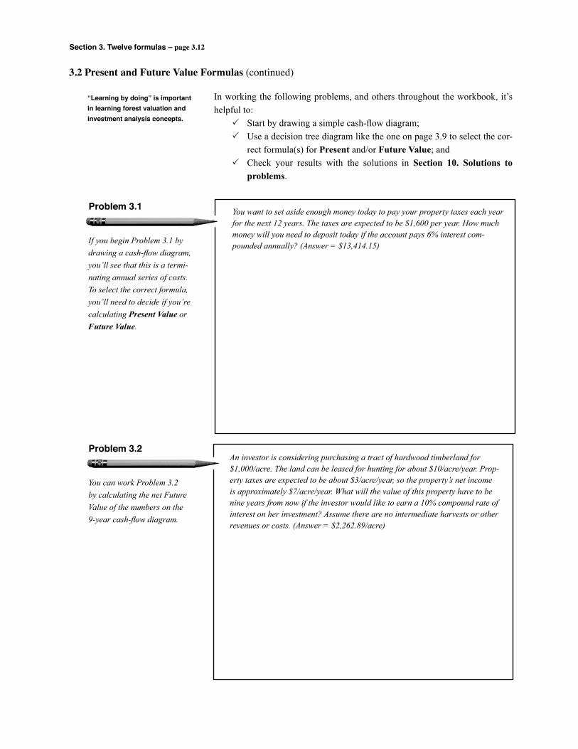
Section 3. Twelve formulas – page 3.12
If you begin Problem 3.1 by drawing a cash-flow diagram, you’ll see that this is a termi-nating annual series of costs. To select the correct formula, you’ll need to decide if you’re calculating Present Value or Future Value.
Problem 3.1
3.2 Present and Future Value Formulas (continued)
You want to set aside enough money today to pay your property taxes each year for the next 12 years. The taxes are expected to be $1,600 per year. How much money will you need to deposit today if the account pays 6% interest com-pounded annually? (Answer = $13,414.15)
In working the following problems, and others throughout the workbook, it’s helpful to: P Start by drawing a simple cash-flow diagram; P �Use a decision tree diagram like the one on page 3.9 to select the cor-
rect formula(s) for Present and/or Future Value; and P �Check your results with the solutions in Section 10. Solutions to
problems.
“Learning by doing” is important in learning forest valuation and investment analysis concepts.
You can work Problem 3.2 by calculating the net Future Value of the numbers on the 9-year cash-flow diagram.
Problem 3.2An investor is considering purchasing a tract of hardwood timberland for $1,000/acre. The land can be leased for hunting for about $10/acre/year. Prop-erty taxes are expected to be about $3/acre/year, so the property’s net income is approximately $7/acre/year. What will the value of this property have to be nine years from now if the investor would like to earn a 10% compound rate of interest on her investment? Assume there are no intermediate harvests or other revenues or costs. (Answer = $2,262.89/acre)
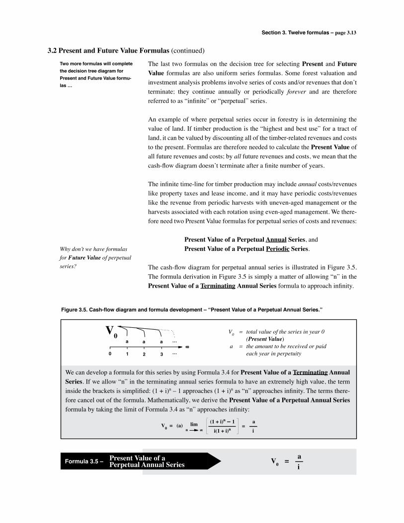
Section 3. Twelve formulas – page 3.13
3.2 Present and Future Value Formulas (continued)
The last two formulas on the decision tree for selecting Present and Future Value formulas are also uniform series formulas. Some forest valuation and investment analysis problems involve series of costs and/or revenues that don’t terminate; they continue annually or periodically forever and are therefore referred to as “infinite” or “perpetual” series.
An example of where perpetual series occur in forestry is in determining the value of land. If timber production is the “highest and best use” for a tract of land, it can be valued by discounting all of the timber-related revenues and costs to the present. Formulas are therefore needed to calculate the Present Value of all future revenues and costs; by all future revenues and costs, we mean that the cash-flow diagram doesn’t terminate after a finite number of years.
The infinite time-line for timber production may include annual costs/revenues like property taxes and lease income, and it may have periodic costs/revenues like the revenue from periodic harvests with uneven-aged management or the harvests associated with each rotation using even-aged management. We there-fore need two Present Value formulas for perpetual series of costs and revenues:
Present Value of a Perpetual Annual Series, and Present Value of a Perpetual Periodic Series.
The cash-flow diagram for perpetual annual series is illustrated in Figure 3.5. The formula derivation in Figure 3.5 is simply a matter of allowing “n” in the Present Value of a Terminating Annual Series formula to approach infinity.
Two more formulas will complete the decision tree diagram for Present and Future Value formu-las …
Why don’t we have formulas for Future Value of perpetual series?
Figure 3.5. Cash-flow diagram and formula development – “Present Value of a Perpetual Annual Series.”
We can develop a formula for this series by using Formula 3.4 for Present Value of a Terminating Annual Series. If we allow “n” in the terminating annual series formula to have an extremely high value, the term inside the brackets is simplified: (1 + i)n – 1 approaches (1 + i)n as “n” approaches infinity. The terms there-fore cancel out of the formula. Mathematically, we derive the Present Value of a Perpetual Annual Series formula by taking the limit of Formula 3.4 as “n” approaches infinity:
V0 = total value of the series in year 0 (Present Value) a = the amount to be received or paid each year in perpetuity
V0 = (a)(1 + i)n – 1
i(1 + i)nlim
n 8
= a
i
Formula 3.5 – V0 = Present Value of aPerpetual Annual Series V0 = a
i
0 1 2 3 …
8
…a a a
V0
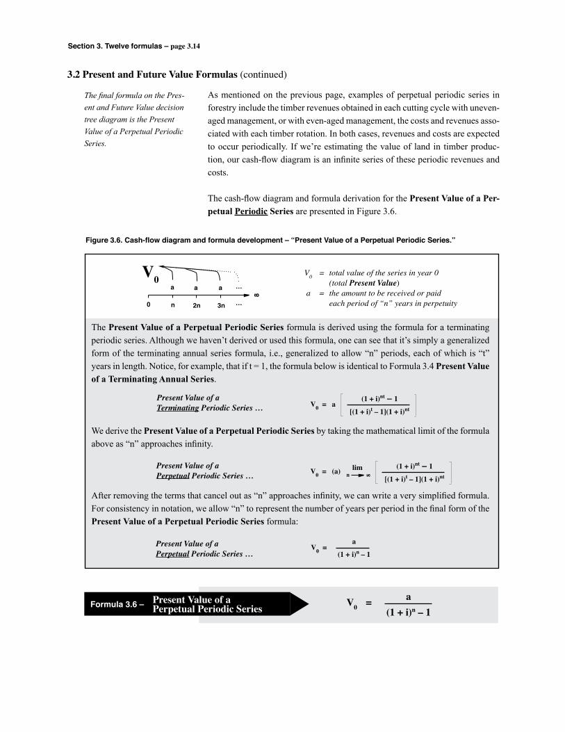
Section 3. Twelve formulas – page 3.14
3.2 Present and Future Value Formulas (continued)
As mentioned on the previous page, examples of perpetual periodic series in forestry include the timber revenues obtained in each cutting cycle with uneven-aged management, or with even-aged management, the costs and revenues asso-ciated with each timber rotation. In both cases, revenues and costs are expected to occur periodically. If we’re estimating the value of land in timber produc-tion, our cash-flow diagram is an infinite series of these periodic revenues and costs.
The cash-flow diagram and formula derivation for the Present Value of a Per-petual Periodic Series are presented in Figure 3.6.
The final formula on the Pres-ent and Future Value decision tree diagram is the Present Value of a Perpetual Periodic Series.
Figure 3.6. Cash-flow diagram and formula development – “Present Value of a Perpetual Periodic Series.”
The Present Value of a Perpetual Periodic Series formula is derived using the formula for a terminating periodic series. Although we haven’t derived or used this formula, one can see that it’s simply a generalized form of the terminating annual series formula, i.e., generalized to allow “n” periods, each of which is “t” years in length. Notice, for example, that if t = 1, the formula below is identical to Formula 3.4 Present Value of a Terminating Annual Series.
We derive the Present Value of a Perpetual Periodic Series by taking the mathematical limit of the formula above as “n” approaches infinity.
After removing the terms that cancel out as “n” approaches infinity, we can write a very simplified formula. For consistency in notation, we allow “n” to represent the number of years per period in the final form of the Present Value of a Perpetual Periodic Series formula:
V0 = total value of the series in year 0 (total Present Value) a = the amount to be received or paid each period of “n” years in perpetuity
V0 = a
(1 + i)n – 1
Formula 3.6 – V0 = Present Value of aPerpetual Periodic Series V0 = a
(1 + i)n – 1
0 n 2n 3n …
8
…a a a
V0
V0 = a(1 + i)nt – 1
[(1 + i)t – 1](1 + i)nt
Present Value of a Terminating Periodic Series …
V0 = (a)(1 + i)nt – 1
[(1 + i)t – 1](1 + i)ntn 8
limPresent Value of a Perpetual Periodic Series …
Present Value of a Perpetual Periodic Series …
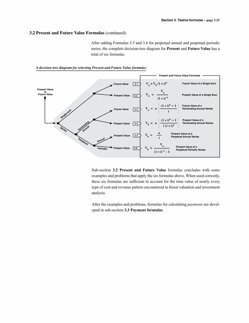
Section 3. Twelve formulas – page 3.15
Vn = V0 (1 + i)n
V0 = Vn
(1 + i) n
Future Value of a Single Sum
Present Value of a Single Sum
Future Value of a Terminating Annual SeriesVn = a
(1 + i)n – 1i
Present Value of a Terminating Annual SeriesV0 = a
(1 + i)n – 1i (1 + i)n
V0 = ai
Present Value of aPerpetual Annual Series
Present and Future Value Formulas
3.1
V0 = Vn
(1 + i) n – 1Present Value of a Perpetual Periodic Series
Future Value
Present Value
Future Value
Present Value
Present Value
Present Value
Series
Single-sum
Present Valueor
Future Value 3.2
3.3
3.4
3.5
3.6
A decision tree diagram for selecting Present and Future Value formulas:
Annual
Periodic
Perpetual
Terminatin
g
Annual
3.2 Present and Future Value Formulas (continued)
After adding Formulas 3.5 and 3.6 for perpetual annual and perpetual periodic series, the complete decision-tree diagram for Present and Future Value has a total of six formulas.
Sub-section 3.2 Present and Future Value formulas concludes with some examples and problems that apply the six formulas above. When used correctly, these six formulas are sufficient to account for the time value of nearly every type of cost and revenue pattern encountered in forest valuation and investment analysis.
After the examples and problems, formulas for calculating payments are devel-oped in sub-section 3.3 Payment formulas.
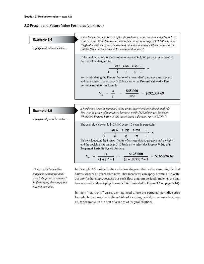
Section 3. Twelve formulas – page 3.16
A perpetual annual series …
Example 3.4 A landowner plans to sell all of his forest-based assets and place the funds in a trust account. If the landowner would like the account to pay $45,000 per year (beginning one year from the deposit), how much money will the assets have to sell for if the account pays 6.5% compound interest?
If the landowner wants the account to provide $45,000 per year in perpetuity, the cash-flow diagram is:
We’re calculating the Present Value of a series that’s perpetual and annual, and the decision tree on page 3.15 leads us to the Present Value of a Per-petual Annual Series formula:
3.2 Present and Future Value Formulas (continued)
0 1 2 3 …
8
…$45K $45K $45K
$45,000.065
V0 = ai
= = $692,307.69
A perpetual periodic series …
Example 3.5 A hardwood forest is managed using group selection silvicultural methods. The tract is expected to produce harvests worth $125,000 every 10 years. What’s the Present Value of this series using a discount rate of 5.75%?
The cash-flow stream is $125,000 every 10 years in perpetuity:
We’re calculating the Present Value of a series that’s perpetual and periodic, and the decision tree on page 3.15 leads us to select the Present Value of a Perpetual Periodic Series formula:
0 10 20 30 …
8
…$125K $125K $125K
$125,000(1 + .0575)10 – 1
= $166,876.67 V0 = a(1 + i)n – 1
=
In Example 3.5, notice in the cash-flow diagram that we’re assuming the first harvest occurs 10 years from now. That means we can apply Formula 3.6 with-out any further steps, because our cash-flow diagram perfectly matches the pat-tern assumed in developing Formula 3.6 (illustrated in Figure 3.6 on page 3.14).
In many “real world” cases, we may need to use the perpetual periodic series formula, but we may be in the middle of a cutting period, or we may be at age 11, for example, in the first of a series of 30-year rotations.
“Real world” cash-flow diagrams sometimes don’t match the patterns assumed in developing the compound interest formulas.
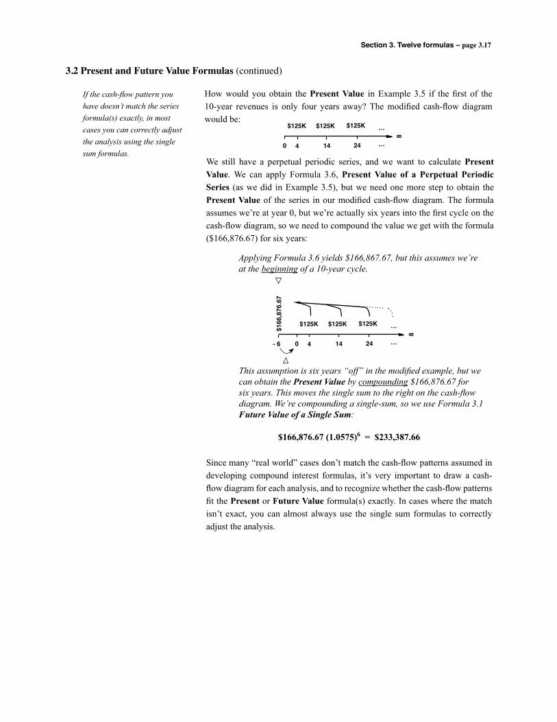
Section 3. Twelve formulas – page 3.17
3.2 Present and Future Value Formulas (continued)
How would you obtain the Present Value in Example 3.5 if the first of the 10-year revenues is only four years away? The modified cash-flow diagram would be:
If the cash-flow pattern you have doesn’t match the series formula(s) exactly, in most cases you can correctly adjust the analysis using the single sum formulas.
We still have a perpetual periodic series, and we want to calculate Present Value. We can apply Formula 3.6, Present Value of a Perpetual Periodic Series (as we did in Example 3.5), but we need one more step to obtain the Present Value of the series in our modified cash-flow diagram. The formula assumes we’re at year 0, but we’re actually six years into the first cycle on the cash-flow diagram, so we need to compound the value we get with the formula ($166,876.67) for six years:
This assumption is six years “off” in the modified example, but we can obtain the Present Value by compounding $166,876.67 for six years. This moves the single sum to the right on the cash-flow diagram. We’re compounding a single-sum, so we use Formula 3.1 Future Value of a Single Sum:
$166,876.67 (1.0575)6 = $233,387.66
Since many “real world” cases don’t match the cash-flow patterns assumed in developing compound interest formulas, it’s very important to draw a cash-flow diagram for each analysis, and to recognize whether the cash-flow patterns fit the Present or Future Value formula(s) exactly. In cases where the match isn’t exact, you can almost always use the single sum formulas to correctly adjust the analysis.
0 4 14 24 …
8
…$125K $125K $125K
0 4 14 24 …
8
…$125K $125K $125K
- 6
$166
,876
.67
Applying Formula 3.6 yields $166,867.67, but this assumes we’reat the beginning of a 10-year cycle.
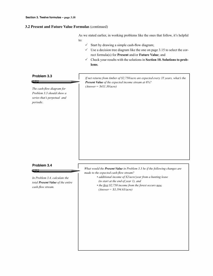
Section 3. Twelve formulas – page 3.18
The cash-flow diagram for Problem 3.3 should show a series that’s perpetual and periodic.
Problem 3.3
3.2 Present and Future Value Formulas (continued)
If net returns from timber of $2,750/acre are expected every 35 years, what’s the Present Value of the expected income stream at 6%? (Answer = $411.30/acre)
As we stated earlier, in working problems like the ones that follow, it’s helpful to: P Start by drawing a simple cash-flow diagram; P Use a decision tree diagram like the one on page 3.15 to select the cor-
rect formula(s) for Present and/or Future Value; and P Check your results with the solutions in Section 10. Solutions to prob-
lems.
In Problem 3.4, calculate the total Present Value of the entire cash-flow stream.
Problem 3.4What would the Present Value in Problem 3.3 be if the following changes are made to the expected cash-flow stream? • additional income of $2/acre/year from a hunting lease (to start at the end of year 1), and • the first $2,750 income from the forest occurs now. (Answer = $3,194.63/acre)

Section 3. Twelve formulas – page 3.19
Your cash-flow diagram should show a series that’s terminating annual …
Problem 3.5
3.2 Present and Future Value Formulas (continued)
Using 10% interest, what’s the Present Value of an 8-year series of property taxes of $3,000 each? Assume the first property tax payment occurs one year from today. (Answer = $16,004.78)
The series formulas assume that the first annual or periodic amount occurs at the end of the first period. In calculating Present Value in this problem, we must recognize that the series formulas don’t account for the value that occurs today, year 0.
Problem 3.6You can lease your land beginning today for the next 25 years for $12/acre per year. How much money is that equivalent to today if your discount rate is 9.5%? What’s the equivalent value today if you can lease the land (beginning today) for $12/acre per year forever? (Answer = $125.25/acre; continuing forever = $138.32/acre)

Section 3. Twelve formulas – page 3.20
Calculate the Present Value of all values on the cash-flow diagram …
Problem 3.7
3.2 Present and Future Value Formulas (continued)
How much money would you need to place in an interest bearing account today if you would like to withdraw $4,000 each year for nine years, and $10,000 after the 10th year? The account earns 7% interest compounded annually. (Answer = $31,144.42)
Determine what the logging firm can afford to pay by calculating the total Present Value of the equipment’s labor savings and salvage value …
Problem 3.8Investing in new equipment is expected to save a logging firm $50,000 per year in labor for each of the next six years. If the firm’s cost of capital is 8%, what can they afford to pay for the new equipment? Assume the equipment is expected to have a salvage value of $60,000 six years from now.(Answer = $268,954.16)
Section 3. Twelve formulas – page 3.21
Calculate the Future Value of a single-sum …
Problem 3.9
3.2 Present and Future Value Formulas (continued)
You recently obtained a high bid of $140,000 for your timber, and you estimate that you can sell the land after harvest for an additional $35,000. If you sell the land and timber and place the $175,000 in a tax-deferred account that earns 5% interest, how much money will be in the account in 25 years? (Answer = $592,612.11)
Determine the total Future Value …
Problem 3.10In Problem 3.9, how much money will be in the account in 25 years if you leave the original $175,000 in the account, and you add $2,000 to the account each year (beginning one year from the original deposit)?(Answer = $688,066.31)
Section 3. Twelve formulas – page 3.22
The value of land for growing timber is the discounted value of all future revenues and costs.
Problem 3.11
3.2 Present and Future Value Formulas (continued)
As a forestry consultant, you have several clients who buy forest properties as investments. Forest lands in different locations vary widely in property taxes levied each year. Using a 9% discount rate, develop a “rule of thumb” for your clients about how differences in property tax levels should impact their bid prices for timberland. That is, how much should a buyer’s offering price be lowered for each dollar of annual property tax on a per acre basis? (Answer = $11.11 per dollar of annual tax liability)
In working Problem 3.12, you’ll need to find the stumpage price projected 10 years from now by compounding today’s price at 2%.
Problem 3.12How much money can you pay now for forest fertilization that will increase your harvest yields by three thousand board feet per acre in 10 years? Stumpage prices in your area today average $420 per thousand board feet, but they are projected to increase by a compound rate of 2% per year. Your cost of capital is 7.5%. (Answer = $745.23/acre)

Section 3. Twelve formulas – page 3.23
Payments are a frequently-encountered example of a uniform series of annual or non-annual expenditures. We include payment formulas in this part of Section 3 because they are encountered so often in forestry and non-forestry applica-tions, and also because they’re used in Section 4 to develop a financial criterion that’s very useful in forestry investment analysis.
There are two types of payments: • Payments to accumulate a specific sum of money over a specific time
period. Such payments are essentially made to yourself, i.e., to your own interest-bearing account. They are sometimes called “sinking fund” payments, with the interest-bearing account referred to as a “sink-ing fund” or “sinking fund” account.
• Payments to repay money that’s borrowed for a specific time period. Examples of such payments include those made on car and truck loans, and home mortgages. Uniform payments to repay an amount borrowed are often called “installment” or “capital recovery” payments.
Payments are sometimes made annually and sometimes they are non-annual. Most examples of non-annual payments are monthly, so in this sub-section we present annual and monthly payment formulas to accumulate a future amount, and to repay an amount borrowed. We therefore present four formulas in a deci-sion tree format :
3.3 Payment formulas
In this part of Section 3 we develop a decision tree dia-gram with four formulas for payments …
Since we’ve already presented six formulas for Present and Future Value, we number the four payment formulas 3.7–3.10.
Payments
3.7 The “sinking fund” formula – annual payments necessary to accumulate a specific future sum.Annual Payment
3.8The “sinking fund” formula – monthly pay-ments necessary to accumulate a specific future sum.
Monthly Payment
3.9Annual Payment
3.10Monthly Payment
Payments to repay
an amount borrowed
The “capital recovery” formula – annual pay-ments necessary to repay a specific amount borrowed.
The “capital recovery” formula – monthly pay-ments necessary to repay a specific amount borrowed.
Payments to accumulate
a future amount
A decision tree diagram can be used to select among four formulas for payments …
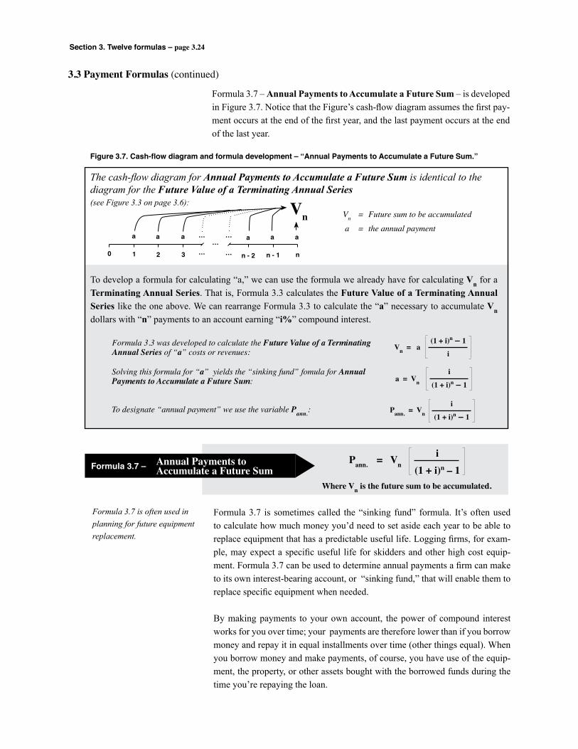
Section 3. Twelve formulas – page 3.24
Formula 3.7 – Annual Payments to Accumulate a Future Sum – is developed in Figure 3.7. Notice that the Figure’s cash-flow diagram assumes the first pay-ment occurs at the end of the first year, and the last payment occurs at the end of the last year.
Formula 3.7 is often used in planning for future equipment replacement.
3.3 Payment Formulas (continued)
0 1 2 3 ……
…
……
n - 1 nn - 2
a a a a aa
Vn
Figure 3.7. Cash-flow diagram and formula development – “Annual Payments to Accumulate a Future Sum.”
The cash-flow diagram for Annual Payments to Accumulate a Future Sum is identical to the diagram for the Future Value of a Terminating Annual Series(see Figure 3.3 on page 3.6):
Vn = Future sum to be accumulated
a = the annual payment
To develop a formula for calculating “a,” we can use the formula we already have for calculating Vn for a Terminating Annual Series. That is, Formula 3.3 calculates the Future Value of a Terminating Annual Series like the one above. We can rearrange Formula 3.3 to calculate the “a” necessary to accumulate Vn dollars with “n” payments to an account earning “i%” compound interest.
Vn = a(1 + i)n – 1
i
Formula 3.7 – V0 = Annual Payments toAccumulate a Future Sum
Pann. = Vni
(1 + i)n – 1
Formula 3.7 is sometimes called the “sinking fund” formula. It’s often used to calculate how much money you’d need to set aside each year to be able to replace equipment that has a predictable useful life. Logging firms, for exam-ple, may expect a specific useful life for skidders and other high cost equip-ment. Formula 3.7 can be used to determine annual payments a firm can make to its own interest-bearing account, or “sinking fund,” that will enable them to replace specific equipment when needed.
By making payments to your own account, the power of compound interest works for you over time; your payments are therefore lower than if you borrow money and repay it in equal installments over time (other things equal). When you borrow money and make payments, of course, you have use of the equip-ment, the property, or other assets bought with the borrowed funds during the time you’re repaying the loan.
Formula 3.3 was developed to calculate the Future Value of a Terminating Annual Series of “a” costs or revenues:
Solving this formula for “a” yields the “sinking fund” fomula for Annual Payments to Accumulate a Future Sum:
To designate “annual payment” we use the variable Pann.: Pann. = Vn i
(1 + i)n – 1
a = Vn i
(1 + i)n – 1
Where Vn is the future sum to be accumulated.
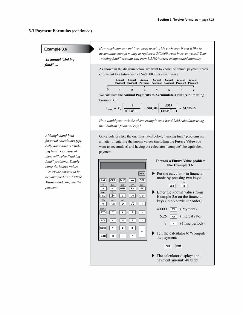
Section 3. Twelve formulas – page 3.25
3.3 Payment Formulas (continued)
2nd CPT DUE +/- OFF
n %i PMT PV FV
ON/C
FRQ ∑+ σn
% 1/x yx ÷
σn-1x
√ x
STO 7 8 9 x
4 5 6 _RCL
1 2 3SUM
0 . =EXC
+
FIN BAL INT APR EFF
STAT ∑ –
∆% lnx e x
DECIMAL
To work a Future Value problemlike Example 3.6:
Put the calculator in financial mode by pressing two keys:
2nd nFIN
Enter the known values fromExample 3.6 on the financial keys (in no particular order):
40000 (Payment)
5.25 (interest rate)
7 (#time periods)n
FV
%i
Tell the calculator to “compute”the payment:
The calculator displays the payment amount: 4875.55
CPT PMT
An annual “sinking fund” …
Example 3.6 How much money would you need to set aside each year if you’d like to accumulate enough money to replace a $40,000 truck in seven years? Your “sinking fund” account will earn 5.25% interest compounded annually.
As shown in the diagram below, we want to know the annual payment that’s equivalent to a future sum of $40,000 after seven years.
We calculate the Annual Payments to Accumulate a Future Sum using Formula 3.7:
How would you work the above example on a hand-held calculator using the “built-in” financial keys?
On calculators like the one illustrated below, “sinking fund” problems are a matter of entering the known values (including the Future Value you want to accumulate) and having the calculator “compute” the equivalent payment.
Although hand-held financial calculators typi-cally don’t have a “sink-ing fund” key, most of them will solve “sinking fund” problems. Simply enter the known values – enter the amount to be accumulated as a Future Value – and compute the payment.
0 1 2 3
AnnualPayment
4 5 6 7
AnnualPayment
AnnualPayment
AnnualPayment
AnnualPayment
AnnualPayment
AnnualPayment
Pann. = Vn i
(1 + i)n – 1= $40,000
.0525
(1.0525)7 – 1= $4,875.55
Section 3. Twelve formulas – page 3.26
Unless stated otherwise, assume the first payment into a “sinking fund” occurs at the end of the first period, and the last payment is at the end of the last period.
Problem 3.13 The owner of a forest property that adjoins your land has said she plans to sell the property eight years from now when she retires. You estimate that the prop-erty will be worth $150,000 in eight years. How much money will you need to place into a “sinking fund” account each year to accumulate $150,000 in eight years? The account pays 6% compounded annually. (Answer = $15,155.39)
The cash-flow diagram for Problem 3.14 should include a series of payments for eight years, and a single sum of $50,000 in year 0.
Problem 3.14How much money would you need to place in an account each year if you’d like to accumulate $150,000 over an eight-year period, and you have $50,000 to place in the account today? The account pays 6% compounded annually. (Answer = $7,103.59)
3.3 Payment Formulas (continued)
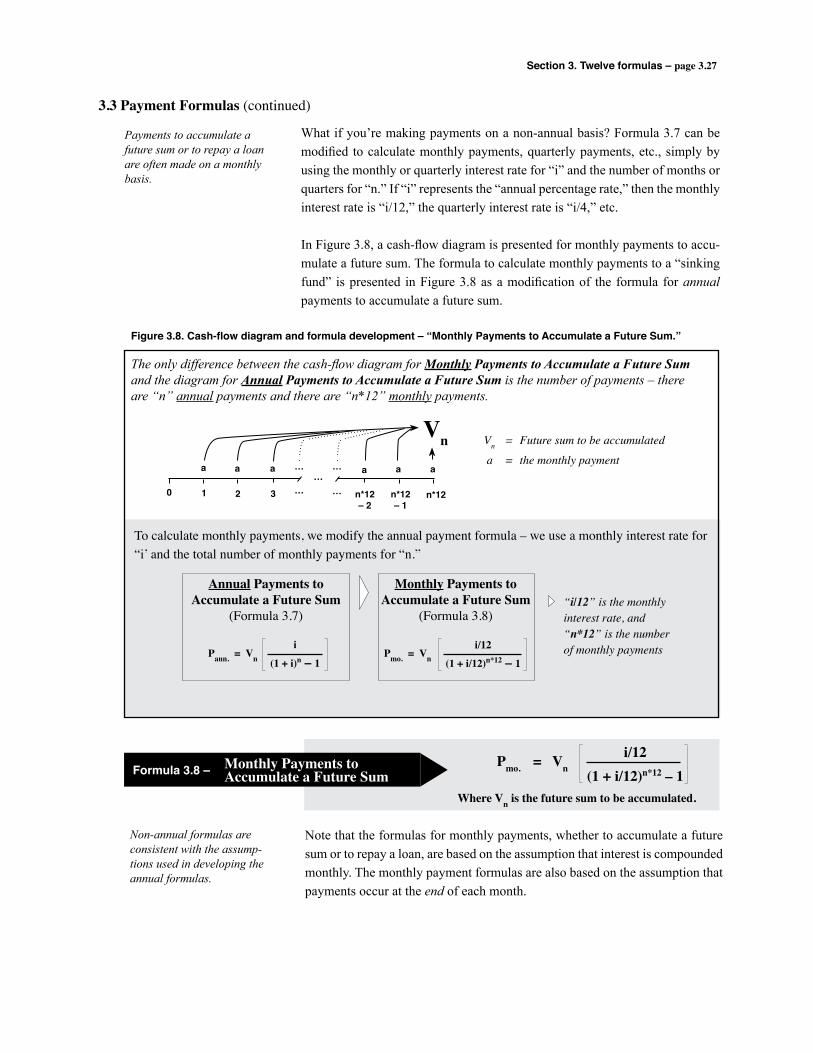
Section 3. Twelve formulas – page 3.27
What if you’re making payments on a non-annual basis? Formula 3.7 can be modified to calculate monthly payments, quarterly payments, etc., simply by using the monthly or quarterly interest rate for “i” and the number of months or quarters for “n.” If “i” represents the “annual percentage rate,” then the monthly interest rate is “i/12,” the quarterly interest rate is “i/4,” etc.
In Figure 3.8, a cash-flow diagram is presented for monthly payments to accu-mulate a future sum. The formula to calculate monthly payments to a “sinking fund” is presented in Figure 3.8 as a modification of the formula for annual payments to accumulate a future sum.
Non-annual formulas are consistent with the assump-tions used in developing the annual formulas.
3.3 Payment Formulas (continued)
Figure 3.8. Cash-flow diagram and formula development – “Monthly Payments to Accumulate a Future Sum.”
The only difference between the cash-flow diagram for Monthly Payments to Accumulate a Future Sum and the diagram for Annual Payments to Accumulate a Future Sum is the number of payments – there are “n” annual payments and there are “n*12” monthly payments.
Vn = Future sum to be accumulated
a = the monthly payment
To calculate monthly payments, we modify the annual payment formula – we use a monthly interest rate for “i’ and the total number of monthly payments for “n.”
Formula 3.8 – V0 = Monthly Payments toAccumulate a Future Sum
Pmo. = Vni/12
(1 + i/12)n*12 – 1
Note that the formulas for monthly payments, whether to accumulate a future sum or to repay a loan, are based on the assumption that interest is compounded monthly. The monthly payment formulas are also based on the assumption that payments occur at the end of each month.
Where Vn is the future sum to be accumulated.
Payments to accumulate a future sum or to repay a loan are often made on a monthly basis.
0 1 2 3 ……
…
……
n*12– 2
a a a a aa
Vn
n*12– 1
n*12
Pann. = Vn i
(1 + i)n – 1
Annual Payments toAccumulate a Future Sum
(Formula 3.7)
Monthly Payments toAccumulate a Future Sum
(Formula 3.8)
Pmo. = Vn i/12
(1 + i/12)n*12 – 1
“i/12” is the monthlyinterest rate, and“n*12” is the numberof monthly payments
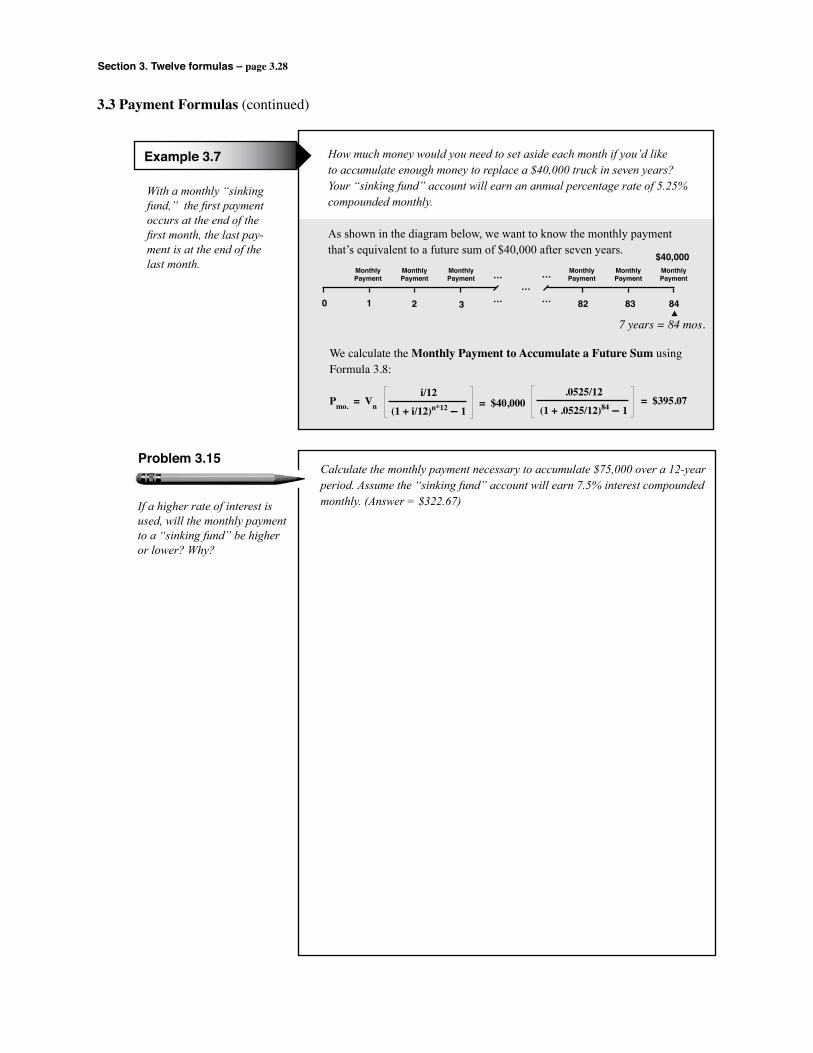
Section 3. Twelve formulas – page 3.28
3.3 Payment Formulas (continued)
With a monthly “sinking fund,” the first payment occurs at the end of the first month, the last pay-ment is at the end of the last month.
Example 3.7 How much money would you need to set aside each month if you’d like to accumulate enough money to replace a $40,000 truck in seven years? Your “sinking fund” account will earn an annual percentage rate of 5.25% compounded monthly.
As shown in the diagram below, we want to know the monthly payment that’s equivalent to a future sum of $40,000 after seven years.
0 1 2 3 82 83 84……
…
……MonthlyPayment
MonthlyPayment
MonthlyPayment
MonthlyPayment
MonthlyPayment
MonthlyPayment
$40,000
We calculate the Monthly Payment to Accumulate a Future Sum using Formula 3.8:
7 years = 84 mos.
Pmo. = Vn i/12
(1 + i/12)n*12 – 1 = $40,000.0525/12
(1 + .0525/12)84 – 1= $395.07
If a higher rate of interest is used, will the monthly payment to a “sinking fund” be higher or lower? Why?
Problem 3.15Calculate the monthly payment necessary to accumulate $75,000 over a 12-year period. Assume the “sinking fund” account will earn 7.5% interest compounded monthly. (Answer = $322.67)
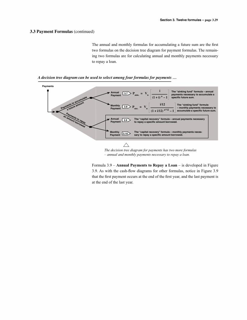
Section 3. Twelve formulas – page 3.29
The decision tree diagram for payments has two more formulas – annual and monthly payments necessary to repay a loan.
The “sinking fund” formula – annual payments necessary to accumulate a specific future sum.
The “sinking fund” formula – monthly payments necessary to accumulate a specific future sum.
AnnualPayment
MonthlyPayment
AnnualPayment
3.7
3.8
3.9
3.10MonthlyPayment
Payments to repay
an amount borrowed
The “capital recovery” formula – annual payments necessary to repay a specific amount borrowed.
The “capital recovery” formula – monthly payments neces-sary to repay a specific amount borrowed.
Payments to accumulate
a future amount
Payments
A decision tree diagram can be used to select among four formulas for payments …
Pann. = Vn i
(1 + i) n – 1
Pmo. = Vn i/12
(1 + i/12) n*12 – 1
3.3 Payment Formulas (continued)
The annual and monthly formulas for accumulating a future sum are the first two formulas on the decision tree diagram for payment formulas. The remain-ing two formulas are for calculating annual and monthly payments necessary to repay a loan.
Formula 3.9 – Annual Payments to Repay a Loan – is developed in Figure 3.9. As with the cash-flow diagrams for other formulas, notice in Figure 3.9 that the first payment occurs at the end of the first year, and the last payment is at the end of the last year.
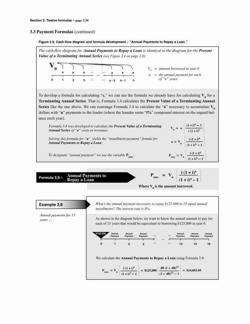
Section 3. Twelve formulas – page 3.30
3.3 Payment Formulas (continued)
Figure 3.9. Cash-flow diagram and formula development – “Annual Payments to Repay a Loan.”
The cash-flow diagram for Annual Payments to Repay a Loan is identical to the diagram for the Present Value of a Terminating Annual Series (see Figure 3.4 on page 3.8):
V0 = amount borrowed in year 0
a = the annual payment for each of “n” years
To develop a formula for calculating “a,” we can use the formula we already have for calculating V0 for a Terminating Annual Series. That is, Formula 3.4 calculates the Present Value of a Terminating Annual Series like the one above. We can rearrange Formula 3.4 to calculate the “a” necessary to accumulate V0 dollars with “n” payments to the lender (where the leander earns “i%” compound interest on the unpaid bal-ance each year).
Vn = a(1 + i)n – 1
i (1 + i)nFormula 3.4 was developed to calculate the Present Value of a Terminating Annual Series of “a” costs or revenues:
Solving this formula for “a” yields the “installment payment” fomula for Annual Payments to Repay a Loan:
To designate “annual payment” we use the variable Pann.: Pann. = Vn i (1 + i)n
(1 + i)n – 1
a = Vn i (1 + i)n
(1 + i)n – 1
Formula 3.9 – V0 = Annual Payments toRepay a Loan
Pann. = Vni (1 + i)n
(1 + i)n – 1Where V0 is the amount borrowed.
0 1 2 3 ……
…
……
n - 1 nn - 2
a a a a aa
V0
Annual payments for 15 years …
Example 3.8 What’s the annual payment necessary to repay $125,000 in 15 equal annual installments? The interest rate is 8%.
As shown in the diagram below, we want to know the annual amount to pay for each of 15 years that would be equivalent to borrowing $125,000 in year 0.
0 1 2 3 13 14 15……
…
……AnnualPayment
AnnualPayment
AnnualPayment
AnnualPayment
AnnualPayment
AnnualPayment
$125,000
We calculate the Annual Payments to Repay a Loan using Formula 3.9:
Pann. = Vn i (1 + i)n
(1 + i)n – 1= $125,000
.08 (1 + .08)15
(1 + .08)15 – 1= $14,603.69

Section 3. Twelve formulas – page 3.31
3.3 Payment Formulas (continued)
2nd CPT DUE +/- OFF
n %i PMT PV FV
ON/C
FRQ ∑+ σn
% 1/x yx ÷
σn-1x
√ x
STO 7 8 9 x
4 5 6 _RCL
1 2 3SUM
0 . =EXC
+
FIN BAL INT APR EFF
STAT ∑ –
∆% lnx e x
DECIMAL
To work an annual payment problemlike Example 3.9:
Put the calculator in financial mode by pressing two keys:
2nd nFIN
Enter the known values fromExample 3.9 on the financial keys (in no particular order):
19000 (Present Value)
9 (interest rate)
10 (#time periods)n
PV
%i
Tell the calculator to “compute”the payment:
The calculator displays the payment amount: 2960.58
CPT PMT
Annual payments for 10 years …
Example 3.9 To regenerate your forest land this year will require $19,000. If you borrow that amount and pay 9% compounded annually, what annual payment is necessary to repay the loan in 10 years?
As shown in the diagram below, we want to know the annual payment that’s necessary to repay $19,000 over a 10-year period.
We calculate the Annual Payments to Repay a Loan using Formula 3.9:
How would you work the above example on a hand-held calculator using the “built-in” financial keys?
On models like the one illustrated below, payments necessary to repay a loan are a matter of entering the known values (including the amount bor-rowed as Present Value) and having the calculator “compute” the equiva-lent payment.
0 1 2 3 8 9 10……
…
……AnnualPayment
AnnualPayment
AnnualPayment
AnnualPayment
AnnualPayment
AnnualPayment
$19,000
Pann. = Vn i (1 + i)n
(1 + i)n – 1= $19,000
.09 (1 + .09)10
(1 + .09)10 – 1= $2,960.58

Section 3. Twelve formulas – page 3.32
Unless stated otherwise, assume that the first installment payment is due at the end of the first period.
Problem 3.16 If you borrow $40,000 at 5.25%, what annual payment is necessary to repay the loan in seven years? (Answer = $6,975.55)
With a “sinking fund” you earn interest ; when you borrow money you pay interest.
Problem 3.17To accumulate $40,000 in a “sinking fund” that earns 5.25% compound inter-est, the annual payment is $4,875.55 (see Example 3.6 on page 3.25). Why is this annual payment lower than the annual payment calculated in Problem 3.16?
3.3 Payment Formulas (continued)

Section 3. Twelve formulas – page 3.33
Formula 3.9 can be modified to calculate monthly payments, quarterly pay-ments, etc., by using the monthly or quarterly interest rate for “i” and the total number of payments for “n.”
In Figure 3.10, a cash-flow diagram is presented for monthly payments to repay a loan. The formula to calculate monthly payments is presented in Figure 3.10 as a modification of the formula for annual payments to repay a loan.
3.3 Payment Formulas (continued)
Figure 3.10. Cash-flow diagram and formula development – “Monthly Payments to Repay a Loan.”
The only difference between the cash-flow diagram for Monthly Payments to Repay a Loan and the cash-flow diagram for Annual Payments to Repay a Loan is the number of payments – there are “n” annual payments and there are “n*12” monthly payments.
To calculate monthly payments, we modify the annual payment formula – we use a monthly interest rate for “i’ and the total number of monthly payments for “n.”
There are many examples of monthly installment payments. In many cases, consumers make monthly payments on car and truck loans, for example, as well as on home mortgages. Monthly payments are also frequently used to repay business loans for property and equipment.
Formula 3.10 – V0 = Monthly Payments toRepay a Loan
Pmo. = V0i/12 (1 + i/12)n*12
(1 + i/12)n*12 – 1Where V0 is the amount borrowed.
Monthly payments to repay a loan are a very common example of using compound interest to account for the time value of money.
Pann. = V0 i (1 + i)n
(1 + i)n – 1
Annual Payments toRepay a Loan(Formula 3.9)
Monthly Payments toRepay a Loan(Formula 3.10)
Pmo. = V0 i/12 (1 + i/12)n*12
(1 + i/12)n*12 – 1
“i/12” is the monthlyinterest rate, and“n*12” is the numberof monthly payments
V0 = amount borrowed in year 0
a = the monthly payment for each of “n*12” years0 1 2 3 …
……
……
n*12– 2
a a a a aa
V0
n*12– 1
n*12
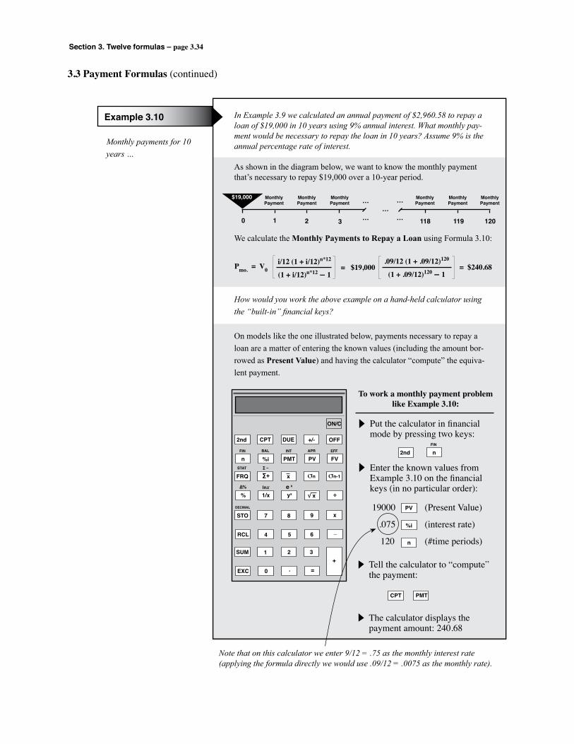
Section 3. Twelve formulas – page 3.34
3.3 Payment Formulas (continued)
2nd CPT DUE +/- OFF
n %i PMT PV FV
ON/C
FRQ ∑+ σn
% 1/x yx ÷
σn-1x
√ x
STO 7 8 9 x
4 5 6 _RCL
1 2 3SUM
0 . =EXC
+
FIN BAL INT APR EFF
STAT ∑ –
∆% lnx e x
DECIMAL
To work a monthly payment problemlike Example 3.10:
Put the calculator in financial mode by pressing two keys:
2nd nFIN
Enter the known values fromExample 3.10 on the financial keys (in no particular order):
19000 (Present Value)
.075 (interest rate)
120 (#time periods)n
PV
%i
Tell the calculator to “compute”the payment:
The calculator displays the payment amount: 240.68
CPT PMT
Monthly payments for 10 years …
Example 3.10 In Example 3.9 we calculated an annual payment of $2,960.58 to repay a loan of $19,000 in 10 years using 9% annual interest. What monthly pay-ment would be necessary to repay the loan in 10 years? Assume 9% is the annual percentage rate of interest.
As shown in the diagram below, we want to know the monthly payment that’s necessary to repay $19,000 over a 10-year period.
We calculate the Monthly Payments to Repay a Loan using Formula 3.10:
How would you work the above example on a hand-held calculator using the “built-in” financial keys?
On models like the one illustrated below, payments necessary to repay a loan are a matter of entering the known values (including the amount bor-rowed as Present Value) and having the calculator “compute” the equiva-lent payment.
0 1 2 3 118 119 120……
…
……MonthlyPayment
MonthlyPayment
MonthlyPayment
MonthlyPayment
MonthlyPayment
MonthlyPayment
$19,000
= $19,000 = $240.68Pmo. = V0 i/12 (1 + i/12)n*12
(1 + i/12)n*12 – 1.09/12 (1 + .09/12)120
(1 + .09/12)120 – 1
Note that on this calculator we enter 9/12 = .75 as the monthly interest rate (applying the formula directly we would use .09/12 = .0075 as the monthly rate).

Section 3. Twelve formulas – page 3.35
In Problem 3.18, compare the monthly payment for a 20-year loan to the payment for a 30-year loan (for the same rate of interest). Is there an interac-tion between the impact of loan length and the rate of interest?
Demand for many forest products is closely related to home building and remodeling. Based on the home mortgages calculated in Problem 3.18, how is the demand for forest products affected by interest rates on home mortgages and home equity loans?
Problem 3.18Calculate the monthly payments for the four home mortgages below. Assume that $100,000 is borrowed.
3.3 Payment Formulas (continued)
i = 12%n = 30 years
(Answer = $1,028.61)
i = 12%n = 20 years
(Answer = $1,101.29)
i = 6%n = 30 years
(Answer = $599.55)
i = 12%n = 20 years
(Answer = $716.43)
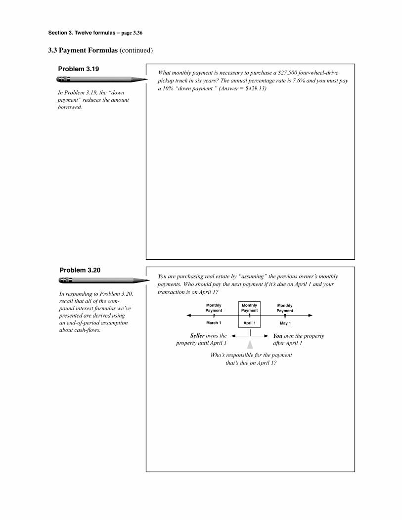
Section 3. Twelve formulas – page 3.36
In Problem 3.19, the “down payment” reduces the amount borrowed.
Problem 3.19 What monthly payment is necessary to purchase a $27,500 four-wheel-drive pickup truck in six years? The annual percentage rate is 7.6% and you must pay a 10% “down payment.” (Answer = $429.13)
In responding to Problem 3.20, recall that all of the com-pound interest formulas we’ve presented are derived using an end-of-period assumption about cash-flows.
Problem 3.20You are purchasing real estate by “assuming” the previous owner’s monthly payments. Who should pay the next payment if it’s due on April 1 and your transaction is on April 1?
3.3 Payment Formulas (continued)
Who’s responsible for the paymentthat’s due on April 1?
MonthlyPayment
MonthlyPayment
MonthlyPayment
May 1April 1March 1
You own the property after April 1
Seller owns theproperty until April 1
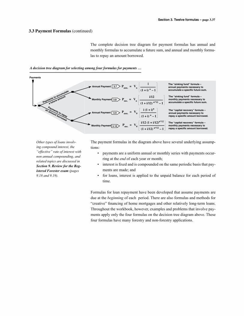
Section 3. Twelve formulas – page 3.37
3.3 Payment Formulas (continued)
The complete decision tree diagram for payment formulas has annual and monthly formulas to accumulate a future sum, and annual and monthly formu-las to repay an amount borrowed.
3.7 Pann. = Vn The “sinking fund” formula –annual payments necessary toaccumulate a specific future sum.
Annual Paymenti
(1 + i) n – 1
The “sinking fund” formula –monthly payments necessary toaccumulate a specific future sum.
Monthly Payment Pmo. = Vn i/12
(1 + i/12) n*12 – 1
Annual Payment
Monthly Payment
Pann. = V0 i (1 + i)n
(1 + i) n – 1
Pmo. = V0 i/12 (1 + i/12)n*12
(1 + i/12) n*12 – 1
Payments to repay
an amount borrowed
The “capital recovery” formula –annual payments necessary torepay a specific amount borrowed.
The “capital recovery” formula –monthly payments necessary torepay a specific amount borrowed.
Payments to accumulate
a future amount
Payments
3.8
3.9
3.10
A decision tree diagram for selecting among four formulas for payments …
The payment formulas in the diagram above have several underlying assump-tions: • payments are a uniform annual or monthly series with payments occur-
ring at the end of each year or month; • interest is fixed and is compounded on the same periodic basis that pay-
ments are made; and • for loans, interest is applied to the unpaid balance for each period of
time.
Formulas for loan repayment have been developed that assume payments are due at the beginning of each period. There are also formulas and methods for “creative” financing of home mortgages and other relatively long-term loans. Throughout the workbook, however, examples and problems that involve pay-ments apply only the four formulas on the decision tree diagram above. These four formulas have many forestry and non-forestry applications.
Other types of loans involv-ing compound interest, the “effective” rate of interest with non annual compounding, and related topics are discussed in Section 9. Review for the Reg-istered Forester exam (pages 9.18 and 9.19).
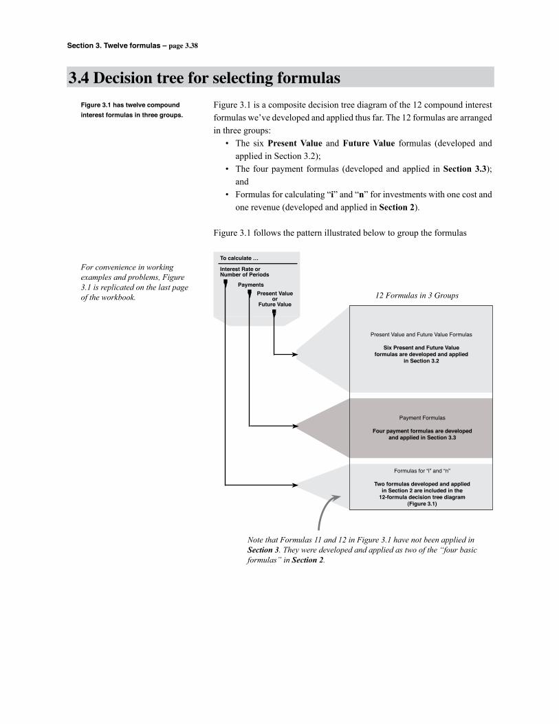
Section 3. Twelve formulas – page 3.38
Figure 3.1 has twelve compound interest formulas in three groups.
Figure 3.1 is a composite decision tree diagram of the 12 compound interest formulas we’ve developed and applied thus far. The 12 formulas are arranged in three groups: • The six Present Value and Future Value formulas (developed and
applied in Section 3.2); • The four payment formulas (developed and applied in Section 3.3);
and • Formulas for calculating “i” and “n” for investments with one cost and
one revenue (developed and applied in Section 2).
Figure 3.1 follows the pattern illustrated below to group the formulas
Present Valueor
Future Value
Payments
To calculate …
Interest Rate orNumber of Periods
Present Value and Future Value Formulas
Six Present and Future Valueformulas are developed and applied
in Section 3.2
12 Formulas in 3 Groups
Payment Formulas
Four payment formulas are developedand applied in Section 3.3
Formulas for “i” and “n”
Two formulas developed and appliedin Section 2 are included in the
12-formula decision tree diagram(Figure 3.1)
3.4 Decision tree for selecting formulas
For convenience in working examples and problems, Figure 3.1 is replicated on the last page of the workbook.
Note that Formulas 11 and 12 in Figure 3.1 have not been applied in Section 3. They were developed and applied as two of the “four basic formulas” in Section 2.
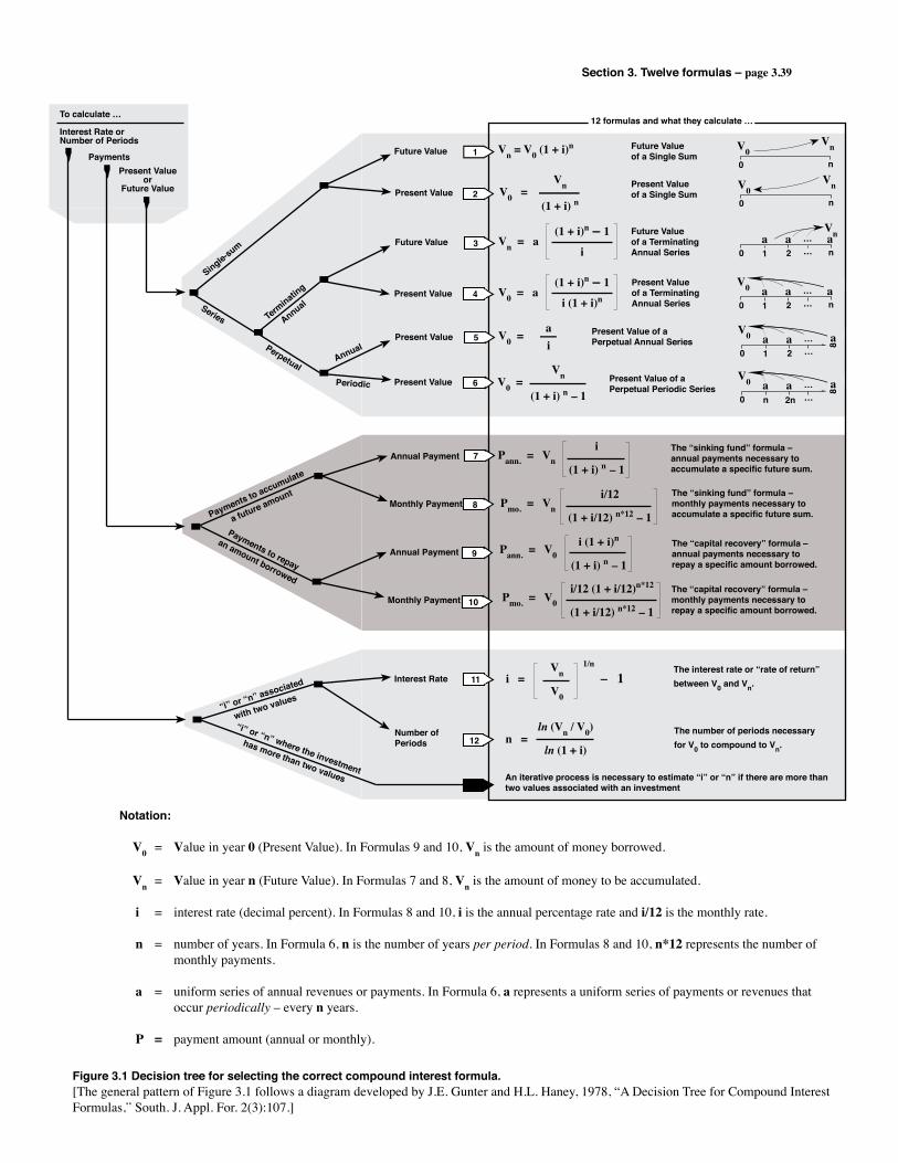
Section 3. Twelve formulas – page 3.39
Vn = V0 (1 + i)n
V0 = Vn
(1 + i) n
Future Valueof a Single Sum
Present Valueof a Single Sum
V0Vn
0 n
V0Vn
0 n
Future Valueof a TerminatingAnnual Series
Vn = a(1 + i)n – 1
i
Vn
0 n1 2 …a a … a
Present Valueof a TerminatingAnnual Series
V0 = a(1 + i)n – 1
i (1 + i)n
V0
0 n1 2 …a a … a
V0 = ai
Present Value of aPerpetual Annual Series
V0
0
8
1 2 …a a … a
12 formulas and what they calculate …
1
2
3
4
5
6 V0 = Vn
(1 + i) n – 1Present Value of a Perpetual Periodic Series
V0
0
8
n 2n …a a … a
Future Value
Present Value
Future Value
Present Value
Present Value
Present Value
Annual
Periodic
Perpetual
Terminatin
g
AnnualSeries
Single-sum
Present Valueor
Future Value
Payments
To calculate …
Interest Rate orNumber of Periods
7 Pann. = Vn The “sinking fund” formula –annual payments necessary toaccumulate a specific future sum.
Annual Paymenti
(1 + i) n – 1
8The “sinking fund” formula –monthly payments necessary toaccumulate a specific future sum.
Monthly Payment Pmo. = Vn i/12
(1 + i/12) n*12 – 1
9Annual Payment
10Monthly Payment
Pann. = V0 i (1 + i)n
(1 + i) n – 1
Pmo. = V0 i/12 (1 + i/12)n*12
(1 + i/12) n*12 – 1
Payments to repay
an amount borrowed
The “capital recovery” formula –annual payments necessary torepay a specific amount borrowed.
The “capital recovery” formula –monthly payments necessary torepay a specific amount borrowed.
Payments to accumulate
a future amount
12Number ofPeriods n =
ln (Vn / V0)
ln (1 + i)
The number of periods necessaryfor V0 to compound to Vn.
“i” or “n” where the investment
has more than two values
“i” or “n” associated
with two values
Interest RateThe interest rate or “rate of return”between V0 and Vn.i = – 1
Vn
V0
1/n
11
An iterative process is necessary to estimate “i” or “n” if there are more thantwo values associated with an investment
Notation:
V0 = Value in year 0 (Present Value). In Formulas 9 and 10, Vn is the amount of money borrowed.
Vn = Value in year n (Future Value). In Formulas 7 and 8, Vn is the amount of money to be accumulated.
i = interest rate (decimal percent). In Formulas 8 and 10, i is the annual percentage rate and i/12 is the monthly rate.
n = number of years. In Formula 6, n is the number of years per period. In Formulas 8 and 10, n*12 represents the number of monthly payments.
a = uniform series of annual revenues or payments. In Formula 6, a represents a uniform series of payments or revenues that occur periodically – every n years.
P = payment amount (annual or monthly).
Figure 3.1 Decision tree for selecting the correct compound interest formula.[The general pattern of Figure 3.1 follows a diagram developed by J.E. Gunter and H.L. Haney, 1978, “A Decision Tree for Compound Interest Formulas,” South. J. Appl. For. 2(3):107.]
Section 3. Twelve formulas – page 3.40
3.1 Introduction The objective of Section 3 was to develop a decision tree diagram for use in
selecting compound interest formulas in later Sections of the workbook.
3.2 Present and Future value formulas Six formulas for calculating Present Value and Future Value were developed
in Section 3.2 and are included on the decision tree diagram of compound interest formulas. These formulas are used in Section 4 to calculate financial criteria like “Net Present Value,” “Rate of Return,” and “Land Expectation Value.”
3.3 Payment formulas Four formulas for calculating payments were developed and are included on
the decision tree diagram. There are actually only two formulas for payments, however, with two versions of each, annual and monthly:
• The “sinking fund” formula (annual and monthly); and • The “capital recovery” or “installment payment” formula (annual and
monthly).
3.3 Decision tree for selecting formulas The composite decision tree diagram (Figure 3.1) has all twelve formulas pre-
sented in three groups. This diagram is intended for use in selecting correct compound interest formulas in later Sections, and for convenience in working problems it’s replicated on the last page of the workbook.
An important reason for emphasizing formula selection and use is that finan-cial calculators have some of the formulas often used in forest valuation and investment analysis, but not all of them. There are many cases where foresters must be able to select and use compound interest formulas directly. Computer programs developed specifically for forestry analysis can also be very helpful; they are presented and discussed in Section 8. Computer programs.
3.5 Review of Section 3
Section 3. Twelve formulas
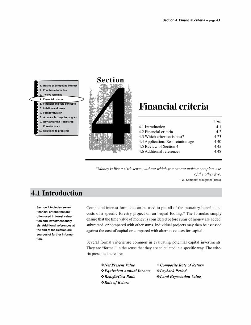
Section 4. Financial criteria – page 4.1
Section
4 Financial criteria
4.1 Introduction 4.14.2 Financial criteria 4.24.3 Which criterion is best? 4.234.4 Application: Best rotation age 4.404.5 Review of Section 4 4.454.6 Additional references 4.48
“Money is like a sixth sense, without which you cannot make a complete use of the other five.
– W. Somerset Maugham (1915)
Compound interest formulas can be used to put all of the monetary benefits and costs of a specific forestry project on an “equal footing.” The formulas simply ensure that the time value of money is considered before sums of money are added, subtracted, or compared with other sums. Individual projects may then be assessed against the cost of capital or compared with alternative uses for capital.
Several formal criteria are common in evaluating potential capital investments. They are “formal” in the sense that they are calculated in a specific way. The crite-ria presented here are:
vNetPresentValue vCompositeRateofReturn vEquivalentAnnualIncome vPaybackPeriod vBenefit/CostRatio vLandExpectationValue vRateofReturn
4.1 Introduction
Page
Section 4 includes seven financial criteria that are often used in forest valua-tion and investment analy-sis. Additional references at the end of the Section are sources of further informa-tion.
1. Basics of compound interest
2. Four basic formulas
3. Twelve formulas
4. Financial criteria
5. Financial analysis concepts
6. Inflation and taxes
7. Forest valuation
8. An example computer program
9. Review for the Registered
Forester exam
10. Solutions to problems
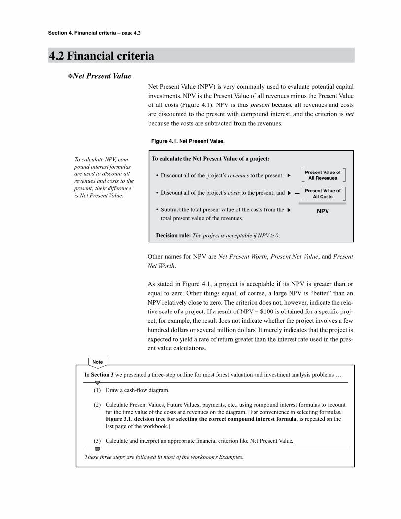
Section 4. Financial criteria – page 4.2
In Section 3 we presented a three-step outline for most forest valuation and investment analysis problems …
(1) Draw a cash-flow diagram.
(2) Calculate Present Values, Future Values, payments, etc., using compound interest formulas to account for the time value of the costs and revenues on the diagram. [For convenience in selecting formulas, Figure 3.1. decision tree for selecting the correct compound interest formula, is repeated on the last page of the workbook.]
(3) Calculate and interpret an appropriate financial criterion like Net Present Value.
These three steps are followed in most of the workbook’s Examples.
To calculate NPV, com-pound interest formulas are used to discount all revenues and costs to the present; their difference is Net Present Value.
Net Present Value (NPV) is very commonly used to evaluate potential capital investments. NPV is the Present Value of all revenues minus the Present Value of all costs (Figure 4.1). NPV is thus present because all revenues and costs are discounted to the present with compound interest, and the criterion is net because the costs are subtracted from the revenues.
Other names for NPV are Net Present Worth, Present Net Value, and Present Net Worth.
As stated in Figure 4.1, a project is acceptable if its NPV is greater than or equal to zero. Other things equal, of course, a large NPV is “better” than an NPV relatively close to zero. The criterion does not, however, indicate the rela-tive scale of a project. If a result of NPV = $100 is obtained for a specific proj-ect, for example, the result does not indicate whether the project involves a few hundred dollars or several million dollars. It merely indicates that the project is expected to yield a rate of return greater than the interest rate used in the pres-ent value calculations.
4.2 Financial criteriavNet Present Value
Figure 4.1. Net Present Value.
To calculate the Net Present Value of a project:
• Discount all of the project’s revenues to the present;
• Discount all of the project’s costs to the present; and
• Subtract the total present value of the costs from the total present value of the revenues.
Decision rule: The project is acceptable if NPV ≥ 0.
Present Value ofAll Revenues
Present Value ofAll Costs
NPV
Note
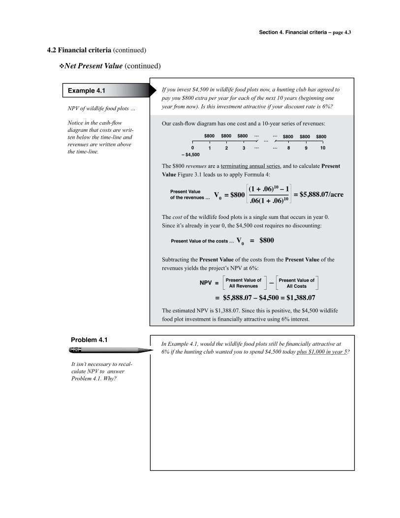
Section 4. Financial criteria – page 4.3
NPV of wildlife food plots …
Notice in the cash-flow diagram that costs are writ-ten below the time-line and revenues are written above the time-line.
Example 4.1 If you invest $4,500 in wildlife food plots now, a hunting club has agreed to pay you $800 extra per year for each of the next 10 years (beginning one year from now). Is this investment attractive if your discount rate is 6%?
Our cash-flow diagram has one cost and a 10-year series of revenues:
The $800 revenues are a terminating annual series, and to calculate Present Value Figure 3.1 leads us to apply Formula 4:
The cost of the wildlife food plots is a single sum that occurs in year 0. Since it’s already in year 0, the $4,500 cost requires no discounting:
Subtracting the Present Value of the costs from the Present Value of the revenues yields the project’s NPV at 6%:
The estimated NPV is $1,388.07. Since this is positive, the $4,500 wildlife food plot investment is financially attractive using 6% interest.
4.2 Financial criteria (continued)
0 1 2 3 ……
…
……
9 108
$800 $800 $800 $800 $800 $800
– $4,500
V0 = $800(1 + .06)10 – 1.06(1 + .06)10
= $5,888.07/acrePresent Valueof the revenues …
Present Value of the costs … V0 = $800
Present Value ofAll Revenues
Present Value ofAll CostsNPV =
= $5,888.07 – $4,500 = $1,388.07
It isn’t necessary to recal-culate NPV to answer Problem 4.1. Why?
Problem 4.1 In Example 4.1, would the wildlife food plots still be financially attractive at 6% if the hunting club wanted you to spend $4,500 today plus $1,000 in year 5?
vNet Present Value (continued)

Section 4. Financial criteria – page 4.4
Equivalent Annual Income (EAI) is another financial criterion that’s frequently used in forest valuation and investment analysis. To calculate EAI for a specific project, first calculate the project’s NPV, then multiply the NPV by the install-ment payment factor, as shown in Figure 4.2.
Calculating EAI is a two-step process. After calculating a project’s NPV, the installment payment formula is used to determine the NPV’s annual equivalent. EAI is simply NPV expressed as an annual amount
The EAI formula is the same as the installment payment formula, so it is in most financial calculators.
EAI is often used to compare forestry returns with pasture rent, agricultural crops, and other land uses that generate income each year.
4.2 Financial criteria (continued)
vEquivalent Annual Income
Figure 4.2. Equivalent Annual Income.
To calculate the Equivalent Annual Income of a project:
(1) Calculate the project’s Net Present Value, as shown in Figure 4.1.
(2) Multiply the NPV by the term in brackets below:
Decision rule: The project is acceptable if EAI ≥ 0. [Note that if NPV is positive, EAI will be positive.]
EAI = NPV i (1 + i)n
(1 + i)n – 1
This formula is identical to the Annual Payments to Repay a Loan formula (forumla 9 in Figure 3.1).
The formula for annual installment payments (Formula 9 in Figure 3.1) calcu-lates payment amounts that are equivalent to a specific amount borrowed, so we can apply the same formula to calculate the annual amount that would be equivalent to a specific NPV.
Since compound interest formulas are used to calculate sums of money that are “equivalent” over time, the name “Equivalent Annual Income” is very appropri-ate for the criterion. Other names for EAI are Annual Equivalent, Equal Annual Equivalent, Annual Income Equivalent, Equal Annual Income, and Net Annual Equivalent.
The EAI criterion is often used to compare or rank investments that are not equal in duration (see page 4.28 in Section 4.3. Which criterion is best?). In many cases, EAI is provided as information in addition to NPV. The concept of an annual income is perhaps more readily understood than the more abstract concept of NPV. Many landowners, for example, can compare the EAI of for-estry investments to annual income from other land uses such as pasture rent or agricultural crops.
The EAI calculation in Figure 4.2 assumes we’ve calculated NPV for a project whose investment life is a finite peri-od of “n” years. The Land Expectation Value (LEV) criterion is a special type of NPV (discussion begins on page 4.18). LEV is calculated assuming an infinite time period and the annual amount that’s equivalent to an LEV is therefore a perpetual annual series. Converting a Land Expectation Value to an EAI is shown on page 4.22.
Note

Section 4. Financial criteria – page 4.5
4.2 Financial criteria (continued)
vEquivalent Annual Income
EAI for a forestry investment …
Note the three steps followed
Example 4.2 In Section1 (page 1.5) we presented an example where the time value of money is sometimes ignored in forestry – timber costs and revenues that are expected during a rotation are sometimes added together and the net amount is divided by the stand’s rotation length. This “annual value” is sometimes presented as the forest landowner’s earnings on a “per acre per year” basis. In the example below, we calculate an “annual income” that ignores the time value of money and we present an “Equivalent Annual Income” for comparison.
What’s the income on a “per acre per year” basis if you completely ignore the time value of money? If we add the revenues, subtract the costs and divide by 30 we obtain $108.33 per acre per year:
When we calculate an EAI, of course, we don’t ignore the time value of money, we explicitly account for it. Following the two steps shown in Figure 4.2 using 7%, for example, yields:
(1) Calculate NPV …
(2) Calculate EAI (by multiplying NPV by the factor in Figure 4.2) …
If we incur the costs and obtain the revenues on the time-line above, during the 30-year rotation our forestry investment will produce returns that are equivalent to an annual income of $32.26/acre.
= $400.33.07 (1.07)30
1.0730 – 1= $32.26/acre/year
Present Value ofAll Revenues
Present Value ofAll CostsNPV =
An example cash-flow diagram for a 30-year rotation:
This is nota valid approach to evaluating forestry investments.
ThinningIncome
$500
Final HarvestIncome$2,900
30160– $150
EstablishmentCost
$500 + $2,900 – $15030 years
= $108.33/acre/year
$500
1.0716
$2,900
1.0730+ – $150
= $400.33/acre
=
EAI = NPV i (1 + i)n
(1 + i)n – 1
Diagram
Calculate
Interpret
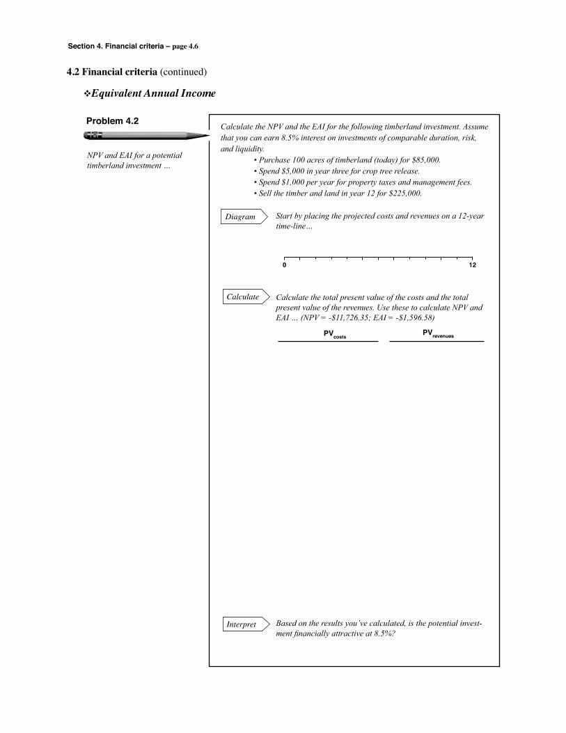
Section 4. Financial criteria – page 4.6
4.2 Financial criteria (continued)
vEquivalent Annual Income
Diagram
Calculate
Interpret
NPV and EAI for a potential timberland investment …
Problem 4.2 Calculate the NPV and the EAI for the following timberland investment. Assume that you can earn 8.5% interest on investments of comparable duration, risk, and liquidity. • Purchase 100 acres of timberland (today) for $85,000. • Spend $5,000 in year three for crop tree release. • Spend $1,000 per year for property taxes and management fees. • Sell the timber and land in year 12 for $225,000.
Start by placing the projected costs and revenues on a 12-year time-line…
Calculate the total present value of the costs and the total present value of the revenues. Use these to calculate NPV and EAI … (NPV = -$11,726.35; EAI = -$1,596.58)
Based on the results you’ve calculated, is the potential invest-ment financially attractive at 8.5%?
0 12
PVcostsPVrevenues
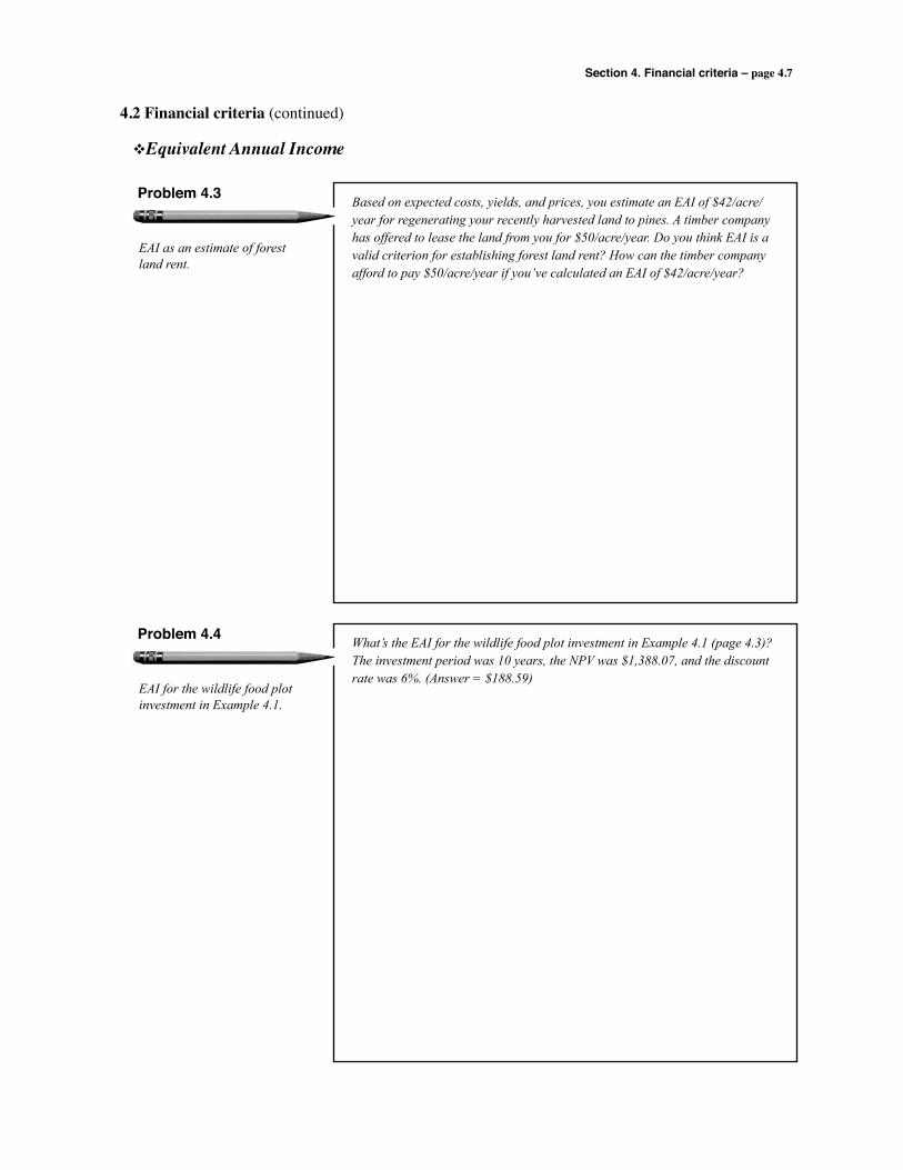
Section 4. Financial criteria – page 4.7
vEquivalent Annual Income
EAI as an estimate of forest land rent.
Problem 4.3 Based on expected costs, yields, and prices, you estimate an EAI of $42/acre/year for regenerating your recently harvested land to pines. A timber company has offered to lease the land from you for $50/acre/year. Do you think EAI is a valid criterion for establishing forest land rent? How can the timber company afford to pay $50/acre/year if you’ve calculated an EAI of $42/acre/year?
4.2 Financial criteria (continued)
EAI for the wildlife food plot investment in Example 4.1.
Problem 4.4 What’s the EAI for the wildlife food plot investment in Example 4.1 (page 4.3)? The investment period was 10 years, the NPV was $1,388.07, and the discount rate was 6%. (Answer = $188.59)
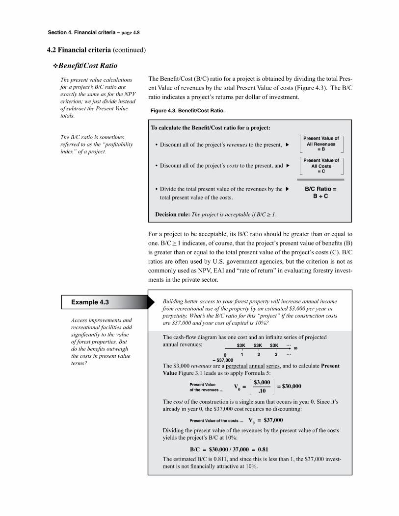
Section 4. Financial criteria – page 4.8
vBenefit/Cost Ratio
4.2 Financial criteria (continued)
The present value calculations for a project’s B/C ratio are exactly the same as for the NPV criterion; we just divide instead of subtract the Present Value totals.
The B/C ratio is sometimes referred to as the “profitability index” of a project.
The Benefit/Cost (B/C) ratio for a project is obtained by dividing the total Pres-ent Value of revenues by the total Present Value of costs (Figure 4.3). The B/C ratio indicates a project’s returns per dollar of investment.
Figure 4.3. Benefit/Cost Ratio.
To calculate the Benefit/Cost ratio for a project:
• Discount all of the project’s revenues to the present,
• Discount all of the project’s costs to the present, and
• Divide the total present value of the revenues by the total present value of the costs.
Decision rule: The project is acceptable if B/C ≥ 1.
B/C Ratio = B ÷ C
Present Value ofAll Revenues
= B
Present Value ofAll Costs
= C
Access improvements and recreational facilities add significantly to the value of forest properties. But do the benefits outweigh the costs in present value terms?
Example 4.3 Building better access to your forest property will increase annual income from recreational use of the property by an estimated $3,000 per year in perpetuity. What’s the B/C ratio for this “project” if the construction costs are $37,000 and your cost of capital is 10%?
The cash-flow diagram has one cost and an infinite series of projected annual revenues:
The $3,000 revenues are a perpetual annual series, and to calculate Present Value Figure 3.1 leads us to apply Formula 5:
The cost of the construction is a single sum that occurs in year 0. Since it’s already in year 0, the $37,000 cost requires no discounting:
Dividing the present value of the revenues by the present value of the costs yields the project’s B/C at 10%:
The estimated B/C is 0.811, and since this is less than 1, the $37,000 invest-ment is not financially attractive at 10%.
V0 = $3,000
.10= $30,000Present Value
of the revenues …
0 1 2 3 …
…$3K $3K $3K
– $37,000
8
Present Value of the costs … V0 = $37,000
B/C = $30,000 / 37,000 = 0.81
For a project to be acceptable, its B/C ratio should be greater than or equal to one. B/C > 1 indicates, of course, that the project’s present value of benefits (B) is greater than or equal to the total present value of the project’s costs (C). B/C ratios are often used by U.S. government agencies, but the criterion is not as commonly used as NPV, EAI and “rate of return” in evaluating forestry invest-ments in the private sector.
Section 4. Financial criteria – page 4.9
vBenefit/Cost Ratio
4.2 Financial criteria (continued)
B/C for a potential timberland investment …
Problem 4.5 Calculate a B/C ratio for Problem 4.2. [Note that if you worked Problem 4.2, you’ve already calculated the present values necessary to calculate the invest-ment’s B/C ratio.]
Financial criteria and the accept/reject decision …
Problem 4.6 If you’re evaluating whether a specific investment is acceptable, will NPV, EAI, and B/C ever “disagree?” Can NPV and EAI be positive (acceptable) for a specific project, for example, while the project’s B/C ratio is less than one (unacceptable)?
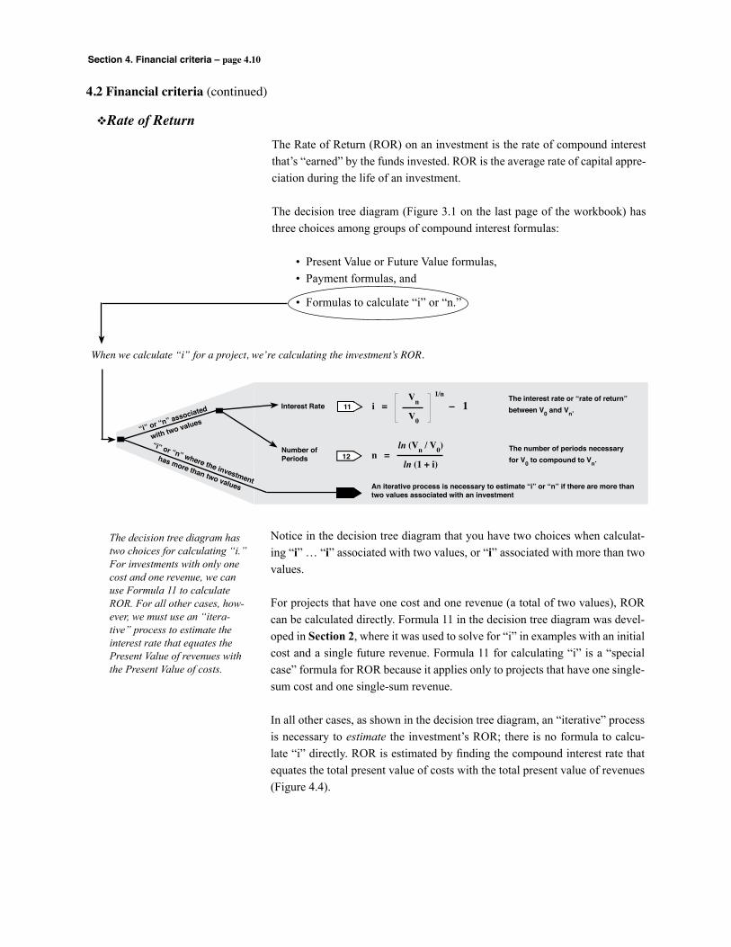
Section 4. Financial criteria – page 4.10
vRate of Return
4.2 Financial criteria (continued)
The Rate of Return (ROR) on an investment is the rate of compound interest that’s “earned” by the funds invested. ROR is the average rate of capital appre-ciation during the life of an investment.
The decision tree diagram (Figure 3.1 on the last page of the workbook) has three choices among groups of compound interest formulas:
• Present Value or Future Value formulas, • Payment formulas, and
• Formulas to calculate “i” or “n.”
When we calculate “i” for a project, we’re calculating the investment’s ROR.
12Number ofPeriods n =
ln (Vn / V0)
ln (1 + i)
The number of periods necessaryfor V0 to compound to Vn.
“i” or “n” where the investment
has more than two values
“i” or “n” associated
with two values
Interest RateThe interest rate or “rate of return”between V0 and Vn.i = – 1
Vn
V0
1/n
11
An iterative process is necessary to estimate “i” or “n” if there are more thantwo values associated with an investment
The decision tree diagram has two choices for calculating “i.” For investments with only one cost and one revenue, we can use Formula 11 to calculate ROR. For all other cases, how-ever, we must use an “itera-tive” process to estimate the interest rate that equates the Present Value of revenues with the Present Value of costs.
Notice in the decision tree diagram that you have two choices when calculat-ing “i” … “i” associated with two values, or “i” associated with more than two values.
For projects that have one cost and one revenue (a total of two values), ROR can be calculated directly. Formula 11 in the decision tree diagram was devel-oped in Section 2, where it was used to solve for “i” in examples with an initial cost and a single future revenue. Formula 11 for calculating “i” is a “special case” formula for ROR because it applies only to projects that have one single-sum cost and one single-sum revenue.
In all other cases, as shown in the decision tree diagram, an “iterative” process is necessary to estimate the investment’s ROR; there is no formula to calcu-late “i” directly. ROR is estimated by finding the compound interest rate that equates the total present value of costs with the total present value of revenues (Figure 4.4).
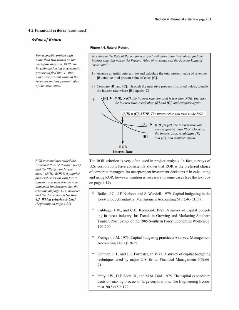
Section 4. Financial criteria – page 4.11
For a specific project with more than two values on the cash-flow diagram, ROR can be estimated using a systematic process to find the “i” that makes the present value of the revenues and the present value of the costs equal.
The ROR criterion is very often used in project analysis. In fact, surveys of U.S. corporations have consistently shown that ROR is the preferred choice of corporate managers for accept/reject investment decisions.* In calculating and using ROR, however, caution is necessary in some cases (see the text box on page 4.14).
* Bailes, J.C., J.F. Nielson, and S. Wendell. 1979. Capital budgeting in the forest products industry. Management Accounting 61(1):46-51, 57.
* Cubbage, F.W., and C.H. Redmond. 1985. A survey of capital budget-ing in forest industry. In: Trends in Growing and Marketing Southern Timber, Proc. Symp. of the 1985 Southern Forest Economics Workers, p. 190-200.
* Fremgen, J.M. 1973. Capital budgeting practices: A survey. Management Accounting 14(11):19-25.
* Gittman, L.J., and J.R. Forrester, Jr. 1977. A survey of capital budgeting techniques used by major U.S. firms. Financial Management 6(3):66-71.
* Petty, J.W., D.F. Scott, Jr., and M.M. Bird. 1975. The capital expenditure decision-making process of large corporations. The Engineering Econo-mist 20(3):159–172.
Figure 4.4. Rate of Return.
To estimate the Rate of Return for a project with more than two values, find the interest rate that makes the Present Value of revenues and the Present Value of costs equal:
1) Assume an initial interest rate and calculate the total present value of revenues [R] and the total present value of costs [C].
2) Compare [R] and [C]. Through the interative process illustrated below, identify the interest rate where [R] equals [C].
vRate of Return
4.2 Financial criteria (continued)
[R]
Interest Rate
[C]
[R]
If [R] > [C], the interest rate you used is less than ROR. Increase the interest rate, recalculate [R] and [C], and compare again.
If [C] > [R], the interest rate you used is greater than ROR. Decrease the interest rate, recalculate [R] and [C], and compare again.
$
If [R] = [C], STOP. The interest rate you used is the ROR.
ROR
ROR is sometimes called the “Internal Rate of Return” (IRR) and the “Return on Invest-ment” (ROI). ROR is a popular financial criterion with forest industry and with private non-industrial landowners. See the cautions on page 4.14, however, and the discussion in Section4.3.Whichcriterionisbest? (beginning on page 4.23).
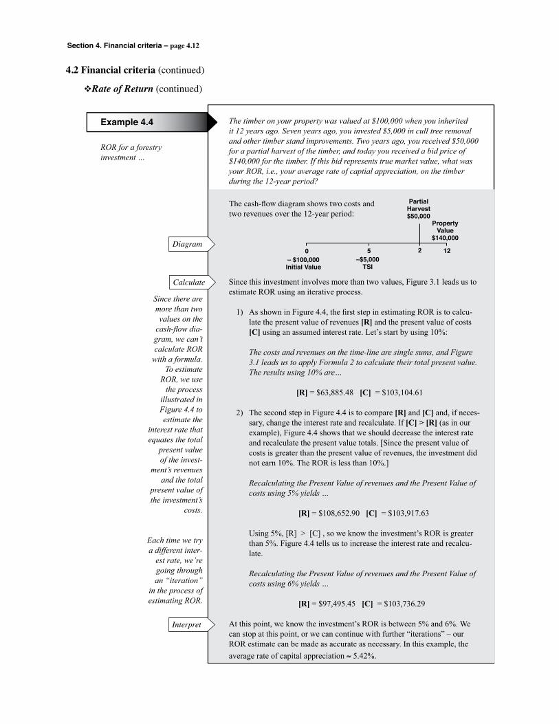
Section 4. Financial criteria – page 4.12
4.2 Financial criteria (continued)
ROR for a forestry investment …
Example 4.4 The timber on your property was valued at $100,000 when you inherited it 12 years ago. Seven years ago, you invested $5,000 in cull tree removal and other timber stand improvements. Two years ago, you received $50,000 for a partial harvest of the timber, and today you received a bid price of $140,000 for the timber. If this bid represents true market value, what was your ROR, i.e., your average rate of captial appreciation, on the timber during the 12-year period?
Since this investment involves more than two values, Figure 3.1 leads us to estimate ROR using an iterative process.
1) As shown in Figure 4.4, the first step in estimating ROR is to calcu-late the present value of revenues [R] and the present value of costs [C] using an assumed interest rate. Let’s start by using 10%:
The costs and revenues on the time-line are single sums, and Figure 3.1 leads us to apply Formula 2 to calculate their total present value. The results using 10% are…
[R] = $63,885.48 [C] = $103,104.61
2) The second step in Figure 4.4 is to compare [R] and [C] and, if neces-sary, change the interest rate and recalculate. If [C] > [R] (as in our example), Figure 4.4 shows that we should decrease the interest rate and recalculate the present value totals. [Since the present value of costs is greater than the present value of revenues, the investment did not earn 10%. The ROR is less than 10%.]
Recalculating the Present Value of revenues and the Present Value of costs using 5% yields …
[R] = $108,652.90 [C] = $103,917.63
Using 5%, [R] > [C] , so we know the investment’s ROR is greater than 5%. Figure 4.4 tells us to increase the interest rate and recalcu-late.
Recalculating the Present Value of revenues and the Present Value of costs using 6% yields …
[R] = $97,495.45 [C] = $103,736.29
At this point, we know the investment’s ROR is between 5% and 6%. We can stop at this point, or we can continue with further “iterations” – our ROR estimate can be made as accurate as necessary. In this example, the average rate of capital appreciation ≈ 5.42%.
The cash-flow diagram shows two costs and two revenues over the 12-year period:
Since there are more than two values on the
cash-flow dia-gram, we can’t calculate ROR
with a formula.To estimate
ROR, we use the process
illustrated in Figure 4.4 to estimate the
interest rate that equates the total
present value of the invest-
ment’s revenues and the total
present value of the investment’s
costs.
Each time we try a different inter-
est rate, we’re going through an “iteration”
in the process of estimating ROR.
vRate of Return (continued)
PartialHarvest$50,000
PropertyValue
$140,000
120– $100,000Initial Value
5–$5,000
TSI
2Diagram
Calculate
Interpret
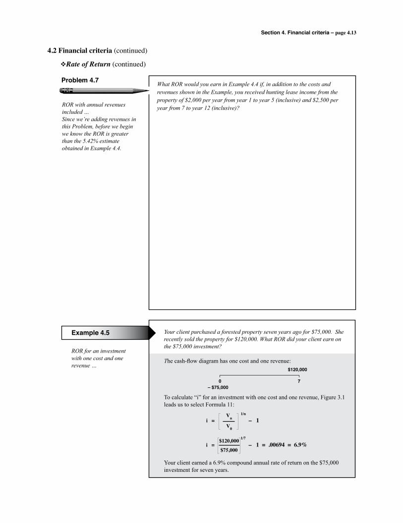
Section 4. Financial criteria – page 4.13
ROR with annual revenues included …Since we’re adding revenues in this Problem, before we begin we know the ROR is greater than the 5.42% estimate obtained in Example 4.4.
Problem 4.7 What ROR would you earn in Example 4.4 if, in addition to the costs and revenues shown in the Example, you received hunting lease income from the property of $2,000 per year from year 1 to year 5 (inclusive) and $2,500 per year from 7 to year 12 (inclusive)?
4.2 Financial criteria (continued)
vRate of Return (continued)
ROR for an investment with one cost and one revenue …
Example 4.5 Your client purchased a forested property seven years ago for $75,000. She recently sold the property for $120,000. What ROR did your client earn on the $75,000 investment?
The cash-flow diagram has one cost and one revenue:
To calculate “i” for an investment with one cost and one revenue, Figure 3.1 leads us to select Formula 11:
Your client earned a 6.9% compound annual rate of return on the $75,000 investment for seven years.
70– $75,000
$120,000
i = – 1 Vn
V0
1/n
i = – 1 = .00694 = 6.9% $120,000
$75,000
1/7
Section 4. Financial criteria – page 4.14
4.2 Financial criteria (continued)
vRate of Return (continued)
• For the ROR criterion to be meaningful, there must be an initial cost, or the costs toward the beginning of the investment must be substantial enough that an average rate of capital appreciation is meaningful. If costs are insignificant, the ROR may be extremely high.
• If an analysis has revenues but costs are excluded entirely, the average rate of capital appreciation is infinite; for this reason, computer pro-grams will “bomb” if you try to calculate an ROR without costs for the investment.
Two common mistakes to avoid – P Foresters sometimes assume (in error) that if timber is sold and some
of the funds are used to pay for reforestation, no cost is involved for new stand establishment. [See Garfitt (1986)*, for example.] This mistake will lead to infinitely high rates of return for the reforesta-tion investment.
P If you’re calculating an ROR for an asset that was inherited or received as a gift, you’ll obtain infinitely high ROR estimates if you assume the initial cost is zero. In reality, such assets have a market value when they’re acquired, and this value is what the current owner has “invested.”
• ROR does not indicate the scale of an investment. Are you earning a 10% ROR on $1 or $1 million?
• In some cases there may be multiple RORs – more than one interest rate at which the Present Value of revenues and the Present Value of costs are equal.
• ROR can be very useful in accept/reject investment decisions; it’s a very widely used criterion for this purpose. ROR is not recommended for ranking investments, however. This is discussed in Section 4.3 Which criterion is best? [See the text box on page 4.28.]
* Garfitt, J.E. 1986. The economic basis of forestry re-examined. Quar. J. For. 80:33–35. [A comment on Garfitt’s article was also published … Price, C. 1986. Will the real case against NDR please step forward? Quar. J. For. 80:159–162.]
When many values are involved in an investment, estimating ROR can be a tedious and time-consuming process. For this reason, computer programs are often used. If you’re estimat-ing ROR with a computer program and the program “aborts” or “bombs” with-out an error message, check to make sure you’ve included all of the investment’s costs.
Some cautions in calculating and using ROR as an investment criterion:
Section 4. Financial criteria – page 4.15
4.2 Financial criteria (continued)
vRate of Return (continued)
The “Rule of 72” is a “rule of thumb” that’s often used in investment analysis.
The “”Rule of 72” – a brief digression …
The “Rule of 72” can be used to estimate the compound rate of interest (or ROR) necessary for a single sum to double in value during a specific time period. The “Rule” can also be used to estimate the number of years necessary for a single sum to double, given a specific ROR. In either case, the estimate is found by using the number 72 in a simple calculation.
The “Rule of 72” can be stated and applied in two ways:
1) If you’d like a single sum to double in value in “n” years, the “Rule of 72” can be used to estimate the rate of return necessary. In this case, the “Rule” is to divide the number 72 by “n.”
Example: If you’d like your timber investment to double in value over the next six years, what rate of compound
annual growth in value will be necessary?
How accurate is this estimate of 12%? We can calculate the “n” necessary for a single sum to double at 12% using Formula 12 in Figure 3.1:
At 12% it would actually take 6.12 years for a single sum to double. Since the stated goal was 6 years, 12% is a good estimate of the necessary ROR.
2) If you expect a single sum to compound in value at a specific rate of interest, the “Rule of 72” can be used to estimate the number of years necessary for the sum to double in value. In this case, the “Rule” is to divide the number 72 by the rate of growth – the ROR.
Example: How long will it take your money to double in a forestry investment that’s expected to earn a 14% compound annual rate of return?
How accurate is this estimate of 5.14 years? We can calculate the “n” necessary for a single sum to double at
14% using Formula 12 in Figure 3.1:
≈ ROR … an estimate of the interest rate necessary for a single sum to double in value in “n” years72n
≈ 12%726
ln (2)ln (1.12)
= 6.12 years …n =
≈ n … an estimate of the number of years necessary for a single sum to double in value at an interest rate = ROR
72ROR
≈ 5.14 years [Note that 72 is divided by 14, not the decimal percent .14.]7214
ln (2)ln (1.14)
= 5.29 years …n = At 14% it would actually take 5.29 years for a single sum to double – compared to the estimate of 5.14 years.
Two references … Blatner, K.A. and W.M. Cross. 1989. Derivation and accuracy of the ‘Rule of 72.’ Int. J. Math. Educ. Sci. Technol. 20(5):723–729.
Cross, W.M. and K.A. Blatner. 1991. ‘Rule of 70’: Extending ‘Rule of 72’ arguments to interest rates with quarterly, monthly, and daily compounding.
Int. J. Math. Educ. Sci. Technol. 22(2):167–176.
Section 4. Financial criteria – page 4.16
4.2 Financial criteria (continued)
vComposite Rate of Return
The Composite Rate of Return is not universally accepted as a valid investment criterion.
From these references, you can see that forest econo-mists have disagreed on the usefulness and validity of the Composite ROR.
The “composite” or “realizable” rate of return has been proposed as an improve-ment over the “internal” rate of return. The composite rate is calculated by: 1) compounding all intermediate cash flows to the end of the investment
period (using an interest rate that reflects the actual or “realizable” poten-tial for reinvestment); and
2) determining the interest rate that will equate the initial costs with the compounded value of the project’s cash flows.
This criterion is mentioned here because it’s presented by some forestry invest-ment analysis computer programs. It’s not universally accepted as a useful and valid criterion for investment analysis, however. *
* Foster, B.B. 1982. Economic nonsense. (Letter to the editor on the Com-posite Rate of Return) J. For. 80(9):566.
* Foster, B.B. and G.N. Brooks. 1983. Rates of return: Internal or compos-ite? (See Harpole 1984) J. For. 81(10):669-670.
* Hansen, B.G. and A.J. Martin. 1983. That nonsensical composite inter-nal rate. (Letter to the editor on the Composite Rate of Return) J. For. 81(7):422.
* Harpole, G.B. 1984. Rates of return: Internal or composite – A response. (See Foster and Brooks, 1983) J. For. 82(9):558-559.
* Klemperer, W.D. 1981a. Interpreting the realizable rate of return. (See Schallau and Wirth 1981 and Klemperer 1981b) J. For. 79(9):616-617.
* Klemperer, W.D. 1981b. Realizable rate of return: A rejoinder. (See Schallau and Wirth 1981 and Klemperer 1981a) J. For. 79(10):673.
* Marty, R.J. 1969. The composite internal rate of return. For. Sci. 16:276-279.
* Schallau, C.H. and M.E. Wirth. 1980. Reinvestment rate and the analysis of forestry enterprises. J. For. 78(12):740-742.
* Schallau, C.H. and M.E. Wirth. 1981. Interpreting the realizable rate of return: A reply. (See Klemperer 1981a and 1981b) J. For. 79(9):618.
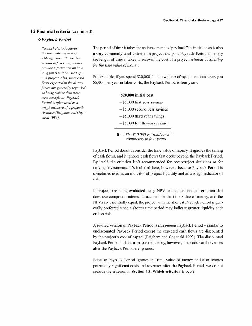
Section 4. Financial criteria – page 4.17
4.2 Financial criteria (continued)
vPayback Period
Payback Period ignores the time value of money. Although the criterion has serious deficiencies, it does provide information on how long funds will be “tied up” in a project. Also, since cash flows expected in the distant future are generally regarded as being riskier than near-term cash flows, Payback Period is often used as a rough measure of a project’s riskiness (Brigham and Gap-enski 1993).
The period of time it takes for an investment to “pay back” its initial costs is also a very commonly used criterion in project analysis. Payback Period is simply the length of time it takes to recover the cost of a project, without accounting for the time value of money.
For example, if you spend $20,000 for a new piece of equipment that saves you $5,000 per year in labor costs, the Payback Period is four years:
$20,000 initial cost
– $5,000 first year savings
– $5,000 second year savings
– $5,000 third year savings
– $5,000 fourth year savings
0 … The $20,000 is “paid back” completely in four years.
Payback Period doesn’t consider the time value of money, it ignores the timing of cash flows, and it ignores cash flows that occur beyond the Payback Period. By itself, the criterion isn’t recommended for accept/reject decisions or for ranking investments. It’s included here, however, because Payback Period is sometimes used as an indicator of project liquidity and as a rough indicator of risk.
If projects are being evaluated using NPV or another financial criterion that does use compound interest to account for the time value of money, and the NPVs are essentially equal, the project with the shortest Payback Period is gen-erally preferred since a shorter time period may indicate greater liquidity and/or less risk.
A revised version of Payback Period is discounted Payback Period – similar to undiscounted Payback Period except the expected cash flows are discounted by the project’s cost of capital (Brigham and Gapenski 1993). The discounted Payback Period still has a serious deficiency, however, since costs and revenues after the Payback Period are ignored.
Because Payback Period ignores the time value of money and also ignores potentially significant costs and revenues after the Payback Period, we do not include the criterion in Section 4.3. Which criterion is best?

Section 4. Financial criteria – page 4.18
4.2 Financial criteria (continued)
vLand Expectation Value
If you estimate the Net Present Value of all cash flows expected from growing timber on a specific tract of land, the expected value of the land has been estimated, hence the name “Land Expectation Value.”
The LEV criterion is also called “Soil Expectation Value” and “Bare Land Value” since many applica-tions assume the cash flow stream begins with bare land. Also, LEV calculations are sometimes referred to as using the “Faustmann formula.” The technique was first published in 1849 by Martin Faustmann, a German appraiser who developed the formula to place values on forest land for property tax purposes.
Land Expectation Value (LEV) is an estimate of the value of a tract of land for growing timber. It is the Net Present Value of all revenues and costs associated with growing timber on the land (not just those associated with one rotation or other time period). LEV is thus a special case of NPV – it’s NPV where all pres-ent and future revenues and costs expected from a tract of land are considered. LEV can be interpreted as the maximum price you can pay for a tract of land for growing timber, if you expect to earn a rate of return greater than or equal to the discount rate used to calculate LEV.
As shown in Figure 4.5, LEV for timber production is calculated assuming the land will be used to produce a perpetual series of even-aged or uneven aged stands; each stand in the perpetual series is assumed to have the same revenues and costs that are projected for the first rotation or the first cutting cycle.
Figure 4.5. Land Expectation Value
To calculate LEV:
1) Determine all of the costs and revenues associated with the first rotation of timber (the first cutting cycle if uneven-aged management is used). These values should include initial costs of planting, site preparation, etc., as well as all subsequent costs and revenues. Land cost should not be included, however. In calculating LEV you’re estimating the value of land for growing timber.
2) Place the first rotation’s (or cutting cycle’s) costs and revenues on a time-line and, using the necessary compound interest formulas, compound all of them to the end of the rotation (or cutting cycle). Subtract the costs from the revenues to obtain a net value at the end of the first period.
3) Assuming a perpetual series of identical n-year rotations (or cutting cycles), the “net value” for the land’s first period can be expected every n years forever…
We therefore calculate “Land Expectation Value” by using the Present Value of a Perpetual Periodic Series formula (Formula 6 in Figure 3.1):
LEV =Net Value in Year n
(1 + i)n – 1
LEV is usually calculated on a per acre basis. It must be calculated for a specific site, for a given species, and assuming a specific management regime and rotation age (even-aged management) or cutting cycle (uneven-aged management).
Costs and Revenues
0 n
Net Valuein year n
0 n
NetValue
3n2n …
NetValue
NetValue
…
8
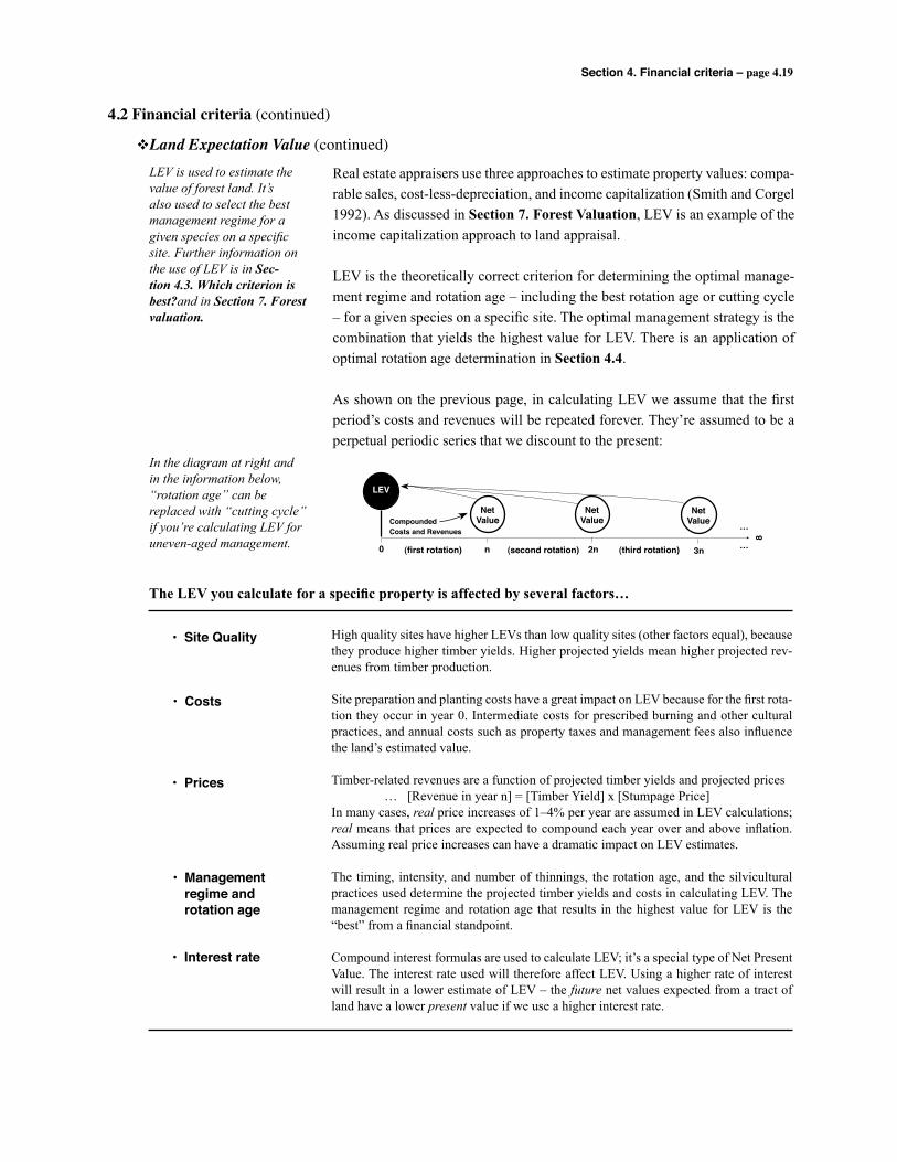
Section 4. Financial criteria – page 4.19
4.2 Financial criteria (continued)
vLand Expectation Value (continued)LEV is used to estimate the value of forest land. It’s also used to select the best management regime for a given species on a specific site. Further information on the use of LEV is in Sec-tion4.3.Whichcriterionisbest?and in Section7.Forestvaluation.
In the diagram at right and in the information below, “rotation age” can be replaced with “cutting cycle” if you’re calculating LEV for uneven-aged management.
Real estate appraisers use three approaches to estimate property values: compa-rable sales, cost-less-depreciation, and income capitalization (Smith and Corgel 1992). As discussed in Section 7. Forest Valuation, LEV is an example of the income capitalization approach to land appraisal.
LEV is the theoretically correct criterion for determining the optimal manage-ment regime and rotation age – including the best rotation age or cutting cycle – for a given species on a specific site. The optimal management strategy is the combination that yields the highest value for LEV. There is an application of optimal rotation age determination in Section 4.4.
As shown on the previous page, in calculating LEV we assume that the first period’s costs and revenues will be repeated forever. They’re assumed to be a perpetual periodic series that we discount to the present:
NetValue
0 n 3n2n
NetValue
NetValue
…
…
8
(first rotation) (second rotation) (third rotation)
CompoundedCosts and Revenues
LEV
High quality sites have higher LEVs than low quality sites (other factors equal), because they produce higher timber yields. Higher projected yields mean higher projected rev-enues from timber production.
Site preparation and planting costs have a great impact on LEV because for the first rota-tion they occur in year 0. Intermediate costs for prescribed burning and other cultural practices, and annual costs such as property taxes and management fees also influence the land’s estimated value.
Timber-related revenues are a function of projected timber yields and projected prices … [Revenue in year n] = [Timber Yield] x [Stumpage Price]In many cases, real price increases of 1–4% per year are assumed in LEV calculations; real means that prices are expected to compound each year over and above inflation. Assuming real price increases can have a dramatic impact on LEV estimates.
The timing, intensity, and number of thinnings, the rotation age, and the silvicultural practices used determine the projected timber yields and costs in calculating LEV. The management regime and rotation age that results in the highest value for LEV is the “best” from a financial standpoint.
Compound interest formulas are used to calculate LEV; it’s a special type of Net Present Value. The interest rate used will therefore affect LEV. Using a higher rate of interest will result in a lower estimate of LEV – the future net values expected from a tract of land have a lower present value if we use a higher interest rate.
The LEV you calculate for a specific property is affected by several factors…
• Site Quality
• Costs
• Prices
• Management regime and rotation age
• Interest rate
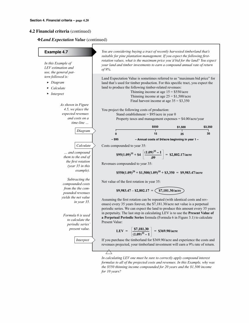
Section 4. Financial criteria – page 4.20
4.2 Financial criteria (continued)
vLand Expectation Value (continued)
In this Example of LEV estimation and use, the general pat-tern followed is: Diagram Calculate Interpret
Example 4.7 You are considering buying a tract of recently harvested timberland that’s suitable for pine plantation management. If you expect the following first-rotation values, what is the maximum price you’d bid for the land? You expect your land and timber investments to earn a compound annual rate of return of 9%.
Land Expectation Value is sometimes referred to as “maximum bid price” for land that’s used for timber production. For this specific tract, you expect the land to produce the following timber-related revenues: Thinning income at age 15 = $550/acre Thinning income at age 25 = $1,500/acre Final harvest income at age 35 = $3,350
You project the following costs of production: Stand establishment = $95/acre in year 0 Property taxes and management expenses = $4.00/acre/year
Costs compounded to year 35:
$95(1.09)35 + $4 = $2,802.17/acre
Revenues compounded to year 35:
$550(1.09)20 + $1,500(1.09)10 + $3,350 = $9,983.47/acre
Net value of the first rotation in year 35:
$9,983.47 – $2,802.17 = $7,181.30/acre
Assuming the first rotation can be repeated (with identical costs and rev-enues) every 35 years forever, the $7,181.30/acre net value is a perpetual periodic series. We can expect the land to produce this amount every 35 years in perpetuity. The last step in calculating LEV is to use the Present Value of a Perpetual Periodic Series formula (Formula 6 in Figure 3.1) to calculate Present Value:
LEV = = $369.90/acre
If you purchase the timberland for $369.90/acre and experience the costs and revenues projected, your timberland investment will earn a 9% rate of return.
In calculating LEV one must be sure to correctly apply compound interest formulas to all of the projected costs and revenues. In this Example, why was the $550 thinning income compounded for 20 years and the $1,500 income for 10 years?
… and compound them to the end of
the first rotation (year 35 in this
example).
Subtracting the compounded costs from the the com-pounded revenues
yields the net value in year 35.
Formula 6 is used to calculate the periodic series’
present value.
(1.09)35 – 1.09
$7,181.30(1.09)35 – 1
As shown in Figure 4.5, we place the
expected revenues and costs on a
time-line …
0 2515
$550 $1,500
35
$3,350
– $95 – Annual costs of $4/acre beginning in year 1 –
Diagram
Calculate
Interpret
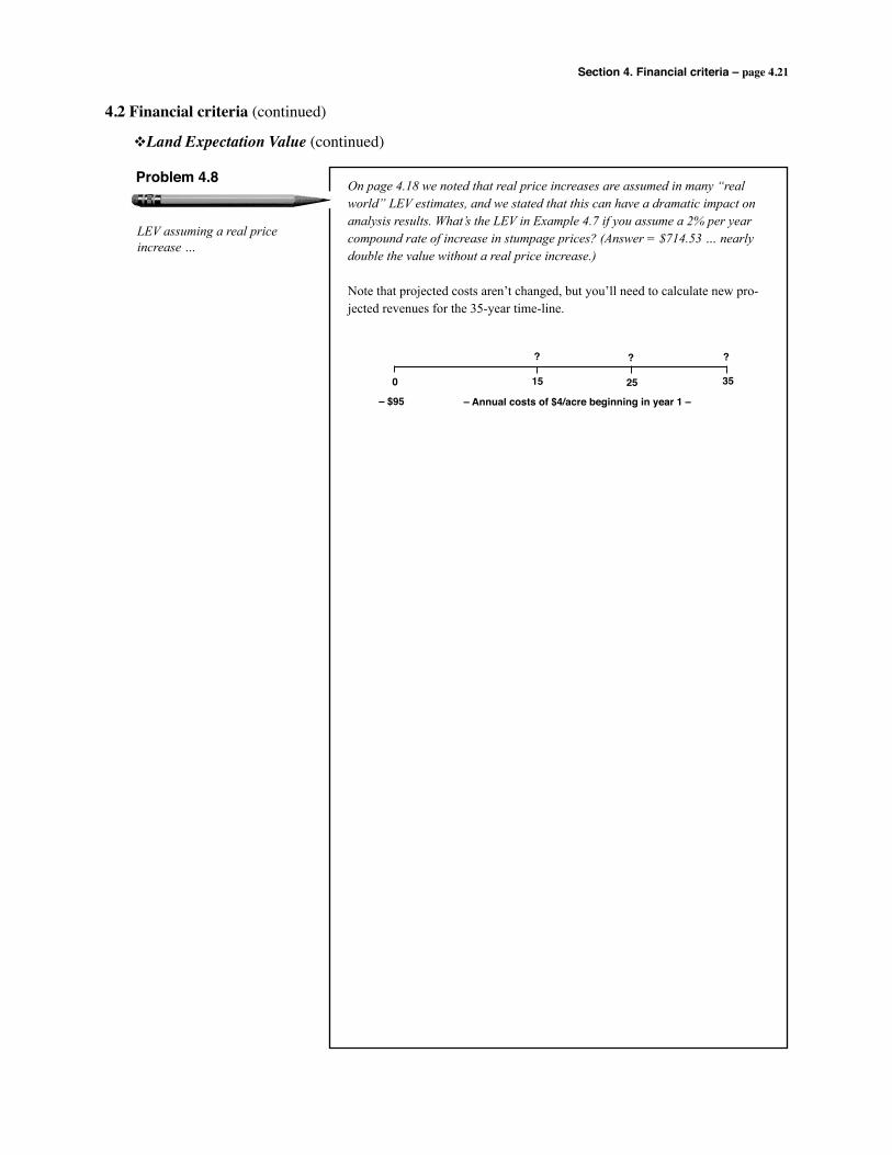
Section 4. Financial criteria – page 4.21
0 2515
?
35
??
– $95 – Annual costs of $4/acre beginning in year 1 –
4.2 Financial criteria (continued)
vLand Expectation Value (continued)
LEV assuming a real price increase …
Problem 4.8 On page 4.18 we noted that real price increases are assumed in many “real world” LEV estimates, and we stated that this can have a dramatic impact on analysis results. What’s the LEV in Example 4.7 if you assume a 2% per year compound rate of increase in stumpage prices? (Answer = $714.53 … nearly double the value without a real price increase.)
Note that projected costs aren’t changed, but you’ll need to calculate new pro-jected revenues for the 35-year time-line.

Section 4. Financial criteria – page 4.22
4.2 Financial criteria (continued)
vLand Expectation Value (continued)To convert an LEV estimate to an equivalent annual income (EAI), simply multi-ply it by the interest rate: EAI = LEV (i).
How would you calculate an annual income that’s equivalent to an LEV? That is how would you calculate an EAI based on an LEV?
When we defined EAI (page 4.4), we noted that the formula in Figure 4.2 applies to the NPV for a project of “n” years, a finite time period:
As calculated above, EAI is simply a finite-period NPV expressed as an annual equivalent. LEV is an NPV that has an infinite time horizon, however, so it wouldn’t be appropriate to convert LEV to an annual equivalent simply by replacing NPV with LEV in the formula above. What we can do, however, is allow “n” in the EAI formula above to approach infinity, and then we can mul-tiply the result by LEV (to convert LEV to EAI).
Taking the mathematical limit of the EAI formula above as “n” approaches infinity cancels all of the terms inside the brackets except “i” in the numerator. The formula to convert an LEV to an EAI is therefore very simple:
EAI = LEV (i)
This formula for EAI also “makes sense” from the standpoint of calculating LEV. For example, if a specific agricultural crop is expected to yield a net income of $25/acre/year in perpetuity, what is the LEV for agricultural use of the land?
LEV = Net Present Value of all future revenues and costs = Net Present Value of a perpetual annual series (Formula 5 in Figure 3.1)
= = $416.67/acre
If you used 6% interest and obtained an LEV estimate of $416.67/acre for any land use (forests, agriculture, etc.), its equivalent annual income would be:
EAI = $416.67 (.06) = $25.00/acre/year
EAI = NPVi (1 + i)n
(1 + i)n – 1
$25.00.06
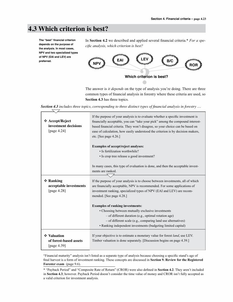
Section 4. Financial criteria – page 4.23
?
In Section 4.2 we described and applied several financial criteria.* For a spe-cific analysis, which criterion is best?
4.3 Which criterion is best?The “best” financial criterion depends on the purpose of the analysis. In most cases, NPV and two specialized types of NPV (EAI and LEV) are preferred.
NPVEAI LEV B/C
ROR
Which criterion is best?
The answer is it depends on the type of analysis you’re doing. There are three common types of financial analysis in forestry where these criteria are used, so Section 4.3 has three topics.
Section 4.3 includes three topics, corresponding to three distinct types of financial analysis in forestry …
v Accept/Reject investment decisions [page 4.24]
v �Ranking acceptable investments [page 4.28]
v �Valuation of forest-based assets [page 4.39]
If the purpose of your analysis is to evaluate whether a specific investment is financially acceptable, you can “take your pick” among the compound interest-based financial criteria. They won’t disagree, so your choice can be based on ease of calculation, how easily understood the criterion is by decision makers, etc. [See page 4.26.]
Examples of accept/reject analyses: • Is fertilization worthwhile? • Is crop tree release a good investment?
In many cases, this type of evaluation is done, and then the acceptable invest-ments are ranked.
If the purpose of your analysis is to choose between investments, all of which are financially acceptable, NPV is recommended. For some applications of investment ranking, specialized types of NPV (EAI and LEV) are recom-mended. [See page 4.28.]
Examples of ranking investments: • Choosing between mutually exclusive investments – of different duration (e.g., optimal rotation age) – of different scale (e.g., comparing land use alternatives) • Ranking independent investments (budgeting limited capital)
If your objective is to estimate a monetary value for forest land, use LEV. Timber valuation is done separately. [Discussion begins on page 4.39.]
“Financial maturity” analysis isn’t listed as a separate type of analysis because choosing a specific stand’s age of final harvest is a form of investment ranking. These concepts are discussed in Section 9. Review for the Registered Forester exam (page 9.6).
* “Payback Period” and “Composite Rate of Return” (CROR) were also defined in Section 4.2. They aren’t included in Section 4.3, however. Payback Period doesn’t consider the time value of money and CROR isn’t fully accepted as a valid criterion for investment analysis.
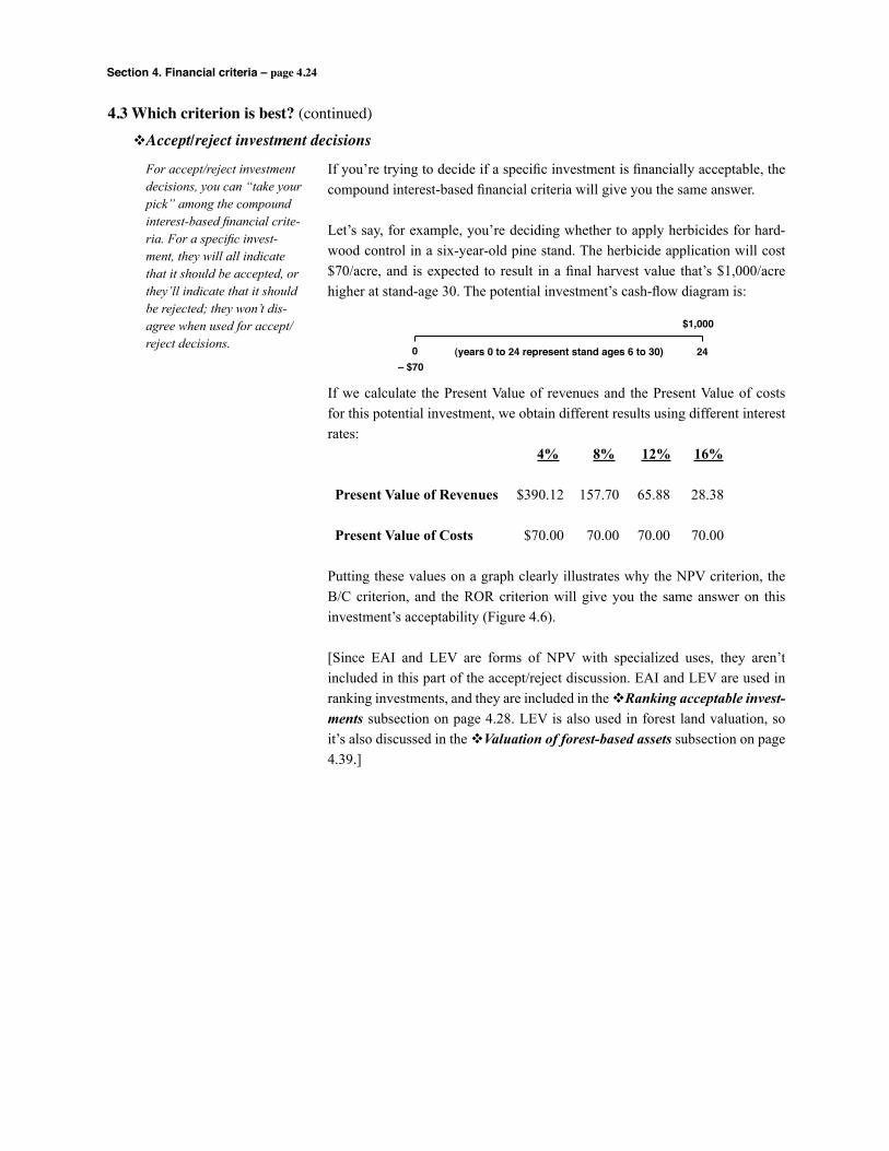
Section 4. Financial criteria – page 4.24
4.3 Which criterion is best? (continued)
vAccept/reject investment decisions
For accept/reject investment decisions, you can “take your pick” among the compound interest-based financial crite-ria. For a specific invest-ment, they will all indicate that it should be accepted, or they’ll indicate that it should be rejected; they won’t dis-agree when used for accept/reject decisions.
If you’re trying to decide if a specific investment is financially acceptable, the compound interest-based financial criteria will give you the same answer.
Let’s say, for example, you’re deciding whether to apply herbicides for hard-wood control in a six-year-old pine stand. The herbicide application will cost $70/acre, and is expected to result in a final harvest value that’s $1,000/acre higher at stand-age 30. The potential investment’s cash-flow diagram is:
If we calculate the Present Value of revenues and the Present Value of costs for this potential investment, we obtain different results using different interest rates: 4% 8% 12% 16%
Present Value of Revenues $390.12 157.70 65.88 28.38
Present Value of Costs $70.00 70.00 70.00 70.00
Putting these values on a graph clearly illustrates why the NPV criterion, the B/C criterion, and the ROR criterion will give you the same answer on this investment’s acceptability (Figure 4.6).
[Since EAI and LEV are forms of NPV with specialized uses, they aren’t included in this part of the accept/reject discussion. EAI and LEV are used in ranking investments, and they are included in the vRankingacceptableinvest-ments subsection on page 4.28. LEV is also used in forest land valuation, so it’s also discussed in the vValuationofforest-basedassets subsection on page 4.39.]
0 – $70
24
$1,000
(years 0 to 24 represent stand ages 6 to 30)
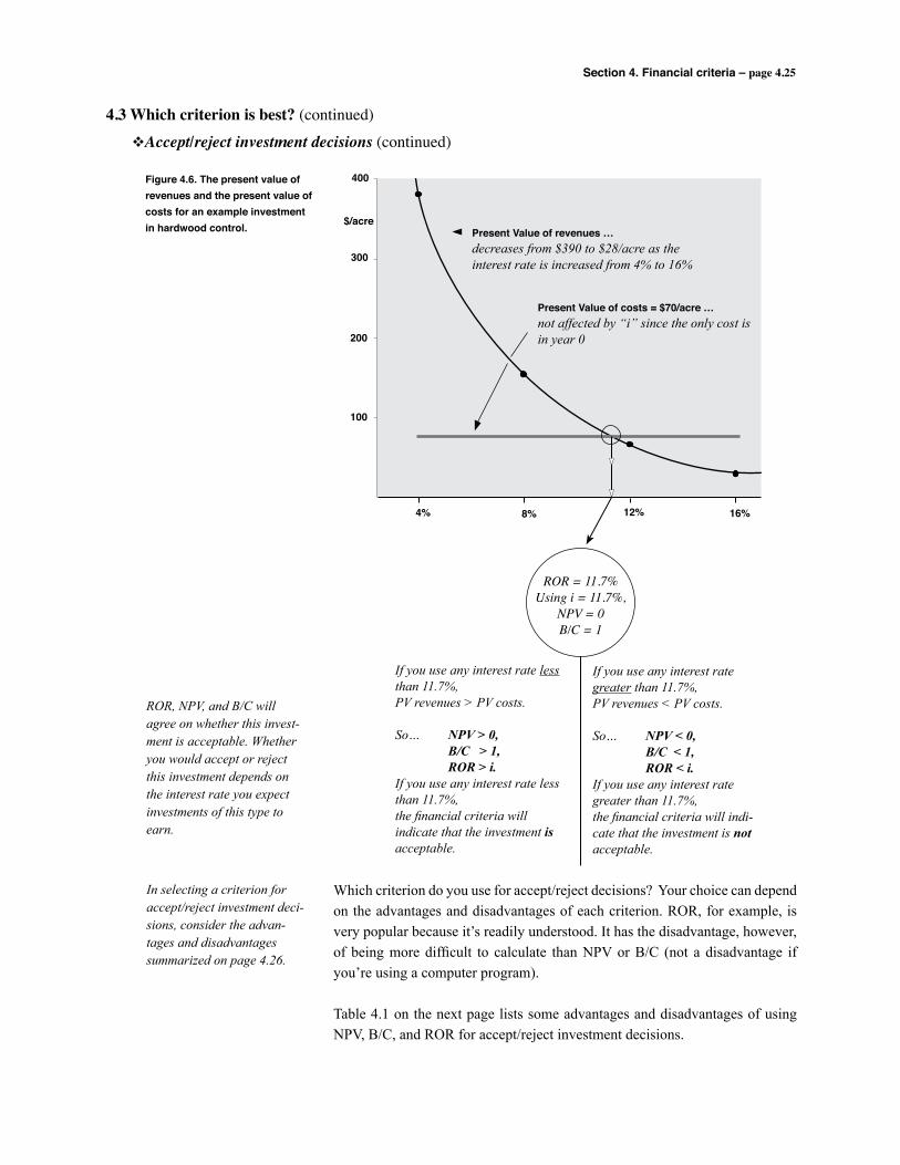
Section 4. Financial criteria – page 4.25
4.3 Which criterion is best? (continued)
vAccept/reject investment decisions (continued)
Figure 4.6. The present value of revenues and the present value of costs for an example investment in hardwood control. $/acre
100
200
300
400
4% 8% 12% 16%
Present Value of revenues …decreases from $390 to $28/acre as the interest rate is increased from 4% to 16%
Present Value of costs = $70/acre …not affected by “i” since the only cost is in year 0
ROR = 11.7%Using i = 11.7%,
NPV = 0B/C = 1
If you use any interest rate less than 11.7%,PV revenues > PV costs.
So… NPV>0, B/C>1, ROR>i.If you use any interest rate less than 11.7%,the financial criteria will indicate that the investment is acceptable.
If you use any interest rate greater than 11.7%,PV revenues < PV costs.
So… NPV<0, B/C<1, ROR<i.If you use any interest rate greater than 11.7%,the financial criteria will indi-cate that the investment is notacceptable.
ROR, NPV, and B/C will agree on whether this invest-ment is acceptable. Whether you would accept or reject this investment depends on the interest rate you expect investments of this type to earn.
Which criterion do you use for accept/reject decisions? Your choice can depend on the advantages and disadvantages of each criterion. ROR, for example, is very popular because it’s readily understood. It has the disadvantage, however, of being more difficult to calculate than NPV or B/C (not a disadvantage if you’re using a computer program).
Table 4.1 on the next page lists some advantages and disadvantages of using NPV, B/C, and ROR for accept/reject investment decisions.
In selecting a criterion for accept/reject investment deci-sions, consider the advan-tages and disadvantages summarized on page 4.26.
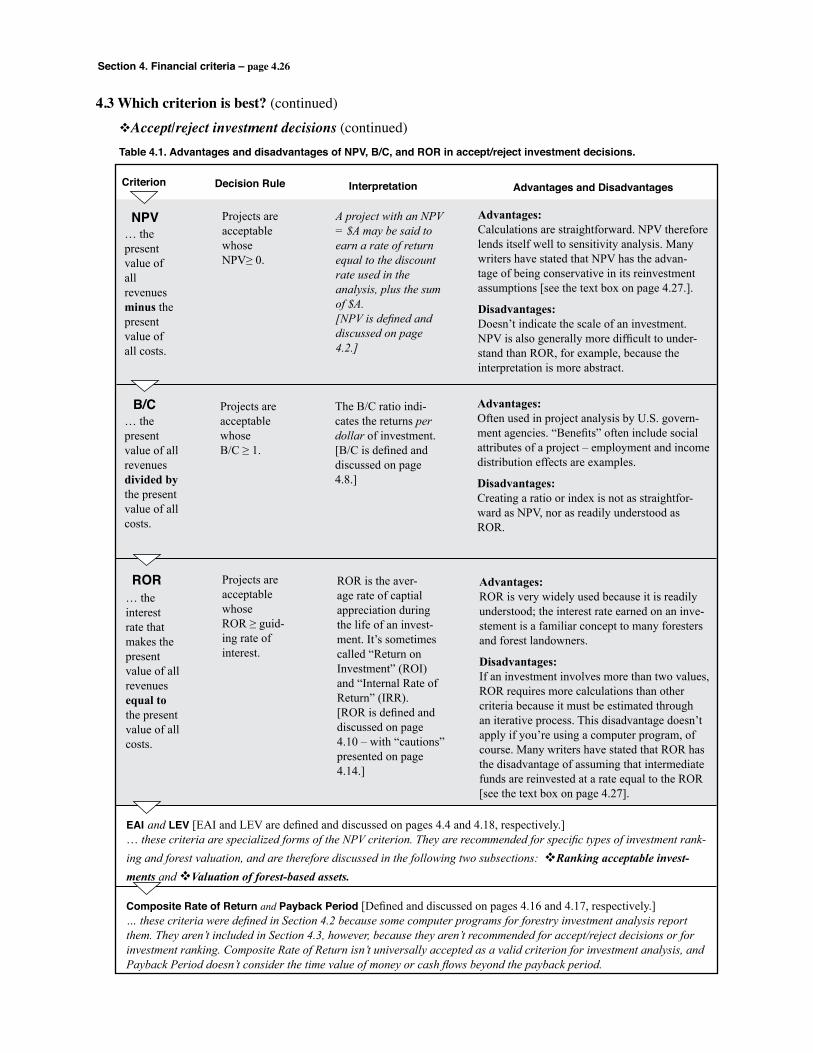
Section 4. Financial criteria – page 4.26
4.3 Which criterion is best? (continued)
vAccept/reject investment decisions (continued)
… thepresentvalue ofallrevenues minus the presentvalue ofall costs.
NPV
Criterion Decision Rule Interpretation Advantages and Disadvantages
Table 4.1. Advantages and disadvantages of NPV, B/C, and ROR in accept/reject investment decisions.
Projects are acceptable whose NPV≥ 0.
A project with an NPV = $A may be said to earn a rate of return equal to the discount rate used in the analysis, plus the sum of $A.[NPV is defined and discussed on page 4.2.]
Advantages:Calculations are straightforward. NPV therefore lends itself well to sensitivity analysis. Many writers have stated that NPV has the advan-tage of being conservative in its reinvestment assumptions [see the text box on page 4.27.].
Disadvantages:Doesn’t indicate the scale of an investment. NPV is also generally more difficult to under-stand than ROR, for example, because the interpretation is more abstract.
… the present value of all revenues divided by the present value of all costs.
B/C
… the interest rate that makes the present value of all revenues equal to the present value of all costs.
ROR Projects are acceptable whose ROR ≥ guid-ing rate of interest.
ROR is the aver-age rate of captial appreciation during the life of an invest-ment. It’s sometimes called “Return on Investment” (ROI) and “Internal Rate of Return” (IRR).[ROR is defined and discussed on page 4.10 – with “cautions” presented on page 4.14.]
Advantages:ROR is very widely used because it is readily understood; the interest rate earned on an inve-stement is a familiar concept to many foresters and forest landowners.
Disadvantages:If an investment involves more than two values, ROR requires more calculations than other criteria because it must be estimated through an iterative process. This disadvantage doesn’t apply if you’re using a computer program, of course. Many writers have stated that ROR has the disadvantage of assuming that intermediate funds are reinvested at a rate equal to the ROR [see the text box on page 4.27].
Projects are acceptable whose B/C ≥ 1.
The B/C ratio indi-cates the returns per dollar of investment.[B/C is defined and discussed on page 4.8.]
Advantages:Often used in project analysis by U.S. govern-ment agencies. “Benefits” often include social attributes of a project – employment and income distribution effects are examples.
Disadvantages:Creating a ratio or index is not as straightfor-ward as NPV, nor as readily understood as ROR.
EAI and LEV [EAI and LEV are defined and discussed on pages 4.4 and 4.18, respectively.]… these criteria are specialized forms of the NPV criterion. They are recommended for specific types of investment rank-ing and forest valuation, and are therefore discussed in the following two subsections: vRankingacceptableinvest-mentsand vValuationofforest-basedassets.
Composite Rate of Return and Payback Period [Defined and discussed on pages 4.16 and 4.17, respectively.]… these criteria were defined in Section 4.2 because some computer programs for forestry investment analysis report them. They aren’t included in Section 4.3, however, because they aren’t recommended for accept/reject decisions or for investment ranking. Composite Rate of Return isn’t universally accepted as a valid criterion for investment analysis, and Payback Period doesn’t consider the time value of money or cash flows beyond the payback period.
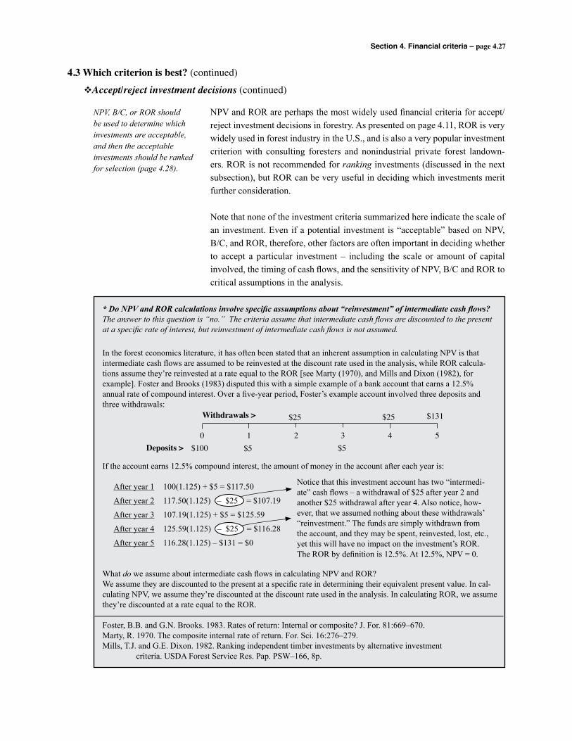
Section 4. Financial criteria – page 4.27
4.3 Which criterion is best? (continued)
vAccept/reject investment decisions (continued)
NPV, B/C, or ROR should be used to determine which investments are acceptable, and then the acceptable investments should be ranked for selection (page 4.28).
NPV and ROR are perhaps the most widely used financial criteria for accept/reject investment decisions in forestry. As presented on page 4.11, ROR is very widely used in forest industry in the U.S., and is also a very popular investment criterion with consulting foresters and nonindustrial private forest landown-ers. ROR is not recommended for ranking investments (discussed in the next subsection), but ROR can be very useful in deciding which investments merit further consideration.
Note that none of the investment criteria summarized here indicate the scale of an investment. Even if a potential investment is “acceptable” based on NPV, B/C, and ROR, therefore, other factors are often important in deciding whether to accept a particular investment – including the scale or amount of capital involved, the timing of cash flows, and the sensitivity of NPV, B/C and ROR to critical assumptions in the analysis.
1 2 3 4 5
$131$25$25
0$100 $5 $5
Withdrawals >
Deposits >
Notice that this investment account has two “intermedi-ate” cash flows – a withdrawal of $25 after year 2 and another $25 withdrawal after year 4. Also notice, how-ever, that we assumed nothing about these withdrawals’ “reinvestment.” The funds are simply withdrawn from the account, and they may be spent, reinvested, lost, etc., yet this will have no impact on the investment’s ROR. The ROR by definition is 12.5%. At 12.5%, NPV = 0.
*DoNPVandRORcalculationsinvolvespecificassumptionsabout“reinvestment”ofintermediatecashflows? The answer to this question is “no.” The criteria assume that intermediate cash flows are discounted to the present at a specific rate of interest, but reinvestment of intermediate cash flows is not assumed. In the forest economics literature, it has often been stated that an inherent assumption in calculating NPV is that intermediate cash flows are assumed to be reinvested at the discount rate used in the analysis, while ROR calcula-tions assume they’re reinvested at a rate equal to the ROR [see Marty (1970), and Mills and Dixon (1982), for example]. Foster and Brooks (1983) disputed this with a simple example of a bank account that earns a 12.5% annual rate of compound interest. Over a five-year period, Foster’s example account involved three deposits and three withdrawals:
If the account earns 12.5% compound interest, the amount of money in the account after each year is:
After year 1 100(1.125) + $5 = $117.50
After year 2 117.50(1.125) – $25 = $107.19
After year 3 107.19(1.125) + $5 = $125.59
After year 4 125.59(1.125) – $25 = $116.28
After year 5 116.28(1.125) – $131 = $0
What do we assume about intermediate cash flows in calculating NPV and ROR? We assume they are discounted to the present at a specific rate in determining their equivalent present value. In cal-culating NPV, we assume they’re discounted at the discount rate used in the analysis. In calculating ROR, we assume they’re discounted at a rate equal to the ROR.
Foster, B.B. and G.N. Brooks. 1983. Rates of return: Internal or composite? J. For. 81:669–670.Marty, R. 1970. The composite internal rate of return. For. Sci. 16:276–279.Mills, T.J. and G.E. Dixon. 1982. Ranking independent timber investments by alternative investment criteria. USDA Forest Service Res. Pap. PSW–166, 8p.
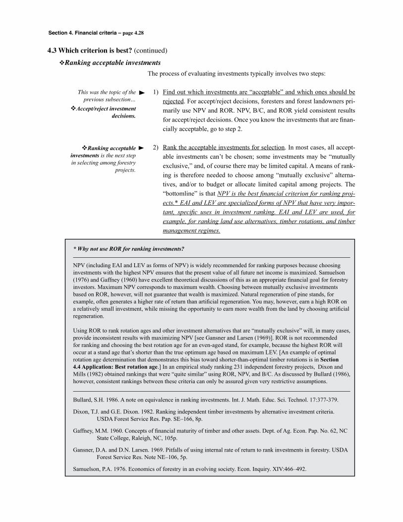
Section 4. Financial criteria – page 4.28
4.3 Which criterion is best? (continued)
vRanking acceptable investments
This was the topic of the previous subsection…
vAccept/rejectinvestmentdecisions.
vRankingacceptableinvestments is the next step in selecting among forestry
projects.
The process of evaluating investments typically involves two steps:
1) Find out which investments are “acceptable” and which ones should be rejected. For accept/reject decisions, foresters and forest landowners pri-marily use NPV and ROR. NPV, B/C, and ROR yield consistent results for accept/reject decisions. Once you know the investments that are finan-cially acceptable, go to step 2.
2) Rank the acceptable investments for selection. In most cases, all accept-able investments can’t be chosen; some investments may be “mutually exclusive,” and, of course there may be limited capital. A means of rank-ing is therefore needed to choose among “mutually exclusive” alterna-tives, and/or to budget or allocate limited capital among projects. The “bottomline” is that NPV is the best financial criterion for ranking proj-ects.* EAI and LEV are specialized forms of NPV that have very impor-tant, specific uses in investment ranking. EAI and LEV are used, for example, for ranking land use alternatives, timber rotations, and timber management regimes.
*WhynotuseRORforrankinginvestments?
NPV (including EAI and LEV as forms of NPV) is widely recommended for ranking purposes because choosing investments with the highest NPV ensures that the present value of all future net income is maximized. Samuelson (1976) and Gaffney (1960) have excellent theoretical discussions of this as an appropriate financial goal for forestry investors. Maximum NPV corresponds to maximum wealth. Choosing between mutually exclusive investments based on ROR, however, will not guarantee that wealth is maximized. Natural regeneration of pine stands, for example, often generates a higher rate of return than artificial regeneration. You may, however, earn a high ROR on a relatively small investment, while missing the opportunity to earn more wealth from the land by choosing artificial regeneration.
Using ROR to rank rotation ages and other investment alternatives that are “mutually exclusive” will, in many cases, provide inconsistent results with maximizing NPV [see Gansner and Larsen (1969)]. ROR is not recommended for ranking and choosing the best rotation age for an even-aged stand, for example, because the highest ROR will occur at a stand age that’s shorter than the true optimum age based on maximum LEV. [An example of optimal rotation age determination that demonstrates this bias toward shorter-than-optimal timber rotations is in Section 4.4 Application: Best rotation age.] In an empirical study ranking 231 independent forestry projects, Dixon and Mills (1982) obtained rankings that were “quite similar” using ROR, NPV, and B/C. As discussed by Bullard (1986), however, consistent rankings between these criteria can only be assured given very restrictive assumptions.
Bullard, S.H. 1986. A note on equivalence in ranking investments. Int. J. Math. Educ. Sci. Technol. 17:377-379.
Dixon, T.J. and G.E. Dixon. 1982. Ranking independent timber investments by alternative investment criteria. USDA Forest Service Res. Pap. SE–166, 8p.
Gaffney, M.M. 1960. Concepts of financial maturity of timber and other assets. Dept. of Ag. Econ. Pap. No. 62, NC State College, Raleigh, NC, 105p.
Gansner, D.A. and D.N. Larsen. 1969. Pitfalls of using internal rate of return to rank investments in forestry. USDA Forest Service Res. Note NE–106, 5p.
Samuelson, P.A. 1976. Economics of forestry in an evolving society. Econ. Inquiry. XIV:466–492.
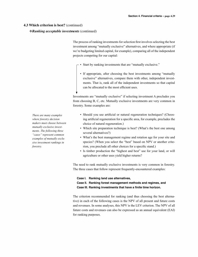
Section 4. Financial criteria – page 4.29
4.3 Which criterion is best? (continued)
vRanking acceptable investments (continued)
There are many examples where forestry decision makers must choose between mutually exclusive invest-ments. The following three “cases” represent common examples of mutually exclu-sive investment rankings in forestry.
The process of ranking investments for selection first involves selecting the best investment among “mutually exclusive” alternatives, and where appropriate (if we’re budgeting limited capital, for example), comparing all of the independent projects competing for our capital: • Start by ranking investments that are “mutually exclusive.”
• If appropriate, after choosing the best investments among “mutually exclusive” alternatives, compare them with other, independent invest-ments. That is, rank all of the independent investments so that capital can be allocated to the most efficient uses.
Investments are “mutually exclusive” if selecting investment A precludes you from choosing B, C, etc. Mutually exclusive investments are very common in forestry. Some examples are:
• Should you use artificial or natural regeneration techniques? (Choos-ing artificial regeneration for a specific area, for example, precludes the choice of natural regeneration.)
• Which site preparation technique is best? (What’s the best one among several alternatives?)
• What’s the best management regime and rotation age for your site and species? (When you select the “best” based on NPV or another crite-rion, you preclude all other choices for a specific stand.)
• Is timber production the “highest and best” use for your land, or will agriculture or other uses yield higher returns?
The need to rank mutually exclusive investments is very common in forestry. The three cases that follow represent frequently-encountered examples:
Case I. Ranking land use alternatives, Case II. Ranking forest management methods and regimes, and Case III. Ranking investments that have a finite time horizon.
The criterion recommended for ranking (and thus choosing the best alterna-tive) in each of the following cases is the NPV of all present and future costs and revenues. In some analyses, this NPV is the LEV criterion. The NPV of all future costs and revenues can also be expressed as an annual equivalent (EAI) for ranking purposes.
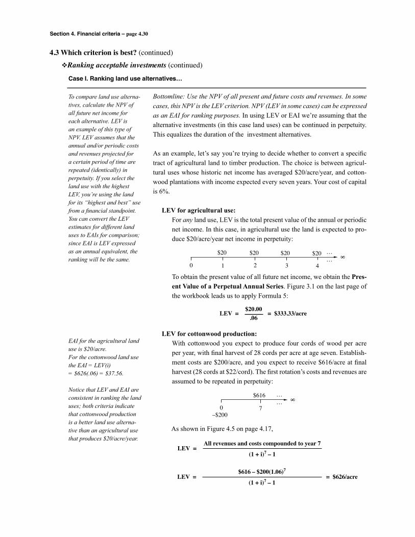
Section 4. Financial criteria – page 4.30
4.3 Which criterion is best? (continued)
vRanking acceptable investments (continued)
To compare land use alterna-tives, calculate the NPV of all future net income for each alternative. LEV is an example of this type of NPV. LEV assumes that the annual and/or periodic costs and revenues projected for a certain period of time are repeated (identically) in perpetuity. If you select the land use with the highest LEV, you’re using the land for its “highest and best” use from a financial standpoint. You can convert the LEV estimates for different land uses to EAIs for comparison; since EAI is LEV expressed as an annual equivalent, the ranking will be the same.
EAI for the agricultural land use is $20/acre. For the cottonwood land use the EAI = LEV(i)= $626(.06) = $37.56.
Notice that LEV and EAI are consistent in ranking the land uses; both criteria indicate that cottonwood production is a better land use alterna-tive than an agricultural use that produces $20/acre/year.
Bottomline: Use the NPV of all present and future costs and revenues. In some cases, this NPV is the LEV criterion. NPV (LEV in some cases) can be expressed as an EAI for ranking purposes. In using LEV or EAI we’re assuming that the alternative investments (in this case land uses) can be continued in perpetuity. This equalizes the duration of the investment alternatives.
As an example, let’s say you’re trying to decide whether to convert a specific tract of agricultural land to timber production. The choice is between agricul-tural uses whose historic net income has averaged $20/acre/year, and cotton-wood plantations with income expected every seven years. Your cost of capital is 6%.
LEV for agricultural use: For any land use, LEV is the total present value of the annual or periodic
net income. In this case, in agricultural use the land is expected to pro-duce $20/acre/year net income in perpetuity:
To obtain the present value of all future net income, we obtain the Pres-
ent Value of a Perpetual Annual Series. Figure 3.1 on the last page of the workbook leads us to apply Formula 5:
LEV for cottonwood production: With cottonwood you expect to produce four cords of wood per acre
per year, with final harvest of 28 cords per acre at age seven. Establish-ment costs are $200/acre, and you expect to receive $616/acre at final harvest (28 cords at $22/cord). The first rotation’s costs and revenues are assumed to be repeated in perpetuity:
As shown in Figure 4.5 on page 4.17,
Case I. Ranking land use alternatives…
0 1 2 3 4
$20 $20 $20 $20 8
……
LEV = = $333.33/acre$20.00
.06
0 7
$616 8
……
–$200
LEV = All revenues and costs compounded to year 7
(1 + i)7 – 1
LEV = = $626/acre $616 – $200(1.06)7
(1 + i)7 – 1
Section 4. Financial criteria – page 4.31
4.3 Which criterion is best? (continued)
vRanking acceptable investments (continued)
Choosing the best even-aged forest management scenario, the best uneven-aged forest management regime, etc., is a choice between mutually exclusive land use alter-natives. From a financial standpoint, the best one has the highest LEV; which can also be expressed as an annual equivalent (EAI). These criteria assume an infinite time-line of projected costs and revenues, and therefore place investments on equal ground in terms of duration.
Based on the information given, cottonwood timber production “outranks” the tract’s agricultural use that generates $20/acre/year. Choosing the best land use alternative for this tract, of course, may involve considering other information – including taxes, sensitivity to assumptions, risk, capital requirements, and other options for how the land is used.
Deciding which set of cultural practices is best, and which management com-bination of thinning regime, rotation length, etc., is best from a financial stand-point is the same as ranking and choosing the best land use alternative. The bottomline is therefore the same one stated in Case I for ranking land use alter-natives (page 4.30).Bottomline: Use the NPV of all present and future costs and revenues. In some cases this NPV is the LEV criterion. NPV (LEV in some cases) can be expressed as an EAI for ranking purposes.
Some specific examples of forest management choices that are mutually exclu-sive:
• Should you use chemical site preparation or mechanical site prepa-ration? These practices have different initial costs and projected timber yields; they may therefore have different optimal rotation ages. Also, the net impact of site preparation practices will depend on site quality, species, planting density, etc. To evaluate the practices, determine the management regime and rotation length that has the highest LEV for each chemical site preparation practice and for each mechanical site preparation practice. The analysis would need to be specific in terms of site quality and spe-cies.
• Should you recommend even-aged management or uneven-aged man-agement? For a given site and species, determine the highest LEV for even-aged management scenarios and compare this to the highest LEV for uneven-aged management.
Case II. Forest management methods and regimes…
Section 4. Financial criteria – page 4.32
4.3 Which criterion is best? (continued)
vRanking acceptable investments (continued)
Pulpwoodvs.sawtimber… in evaluating rotation length choices, if you use the NPV of one rotation (rather than using LEV, which is NPV assuming an infinite series of rotations), you’ll be ignoring the costs and revenues that come after the first rotation. Your analysis won’t recognize the “opportunity costs” of delaying subsequent income, and your analysis will there-fore be biased toward longer rotations. [An example of optimal rotation determina-tion that demonstrates this potential bias is in Section4.4Application:Bestrota-tionage; the “opportunity cost” concept is in Section5.5.]
• Is pulpwood production the “highest and best use” for timberland, or is sawtimber production a better forest management objective? Whether you’re examining this question for hardwood production or softwood pro-duction, for low quality sites or high quality sites, the comparison of final product objectives should be based on obtaining the highest LEV. The alter-native rotations and management scenarios can also be ranked by EAI, since EAI is NPV expressed as an annual equivalent (and since LEV is NPV for an infinite time horizon). EAI will yield the same investment ranking as LEV.
• If you have an existing stand, how do you compare forest management alternatives? That is, you have several management options for the exist-ing stand, but which criterion do you use to determine the one that ranks most highly? By now, of course, you’ve seen that every recommendation (in the above examples) has been to use the NPV of all future costs and revenues.
How do you calculate NPV for all future costs and revenues when you have an existing stand? On the cash-flow diagram for each management alterna-tive, you include all costs and revenues from the current stand, and all costs and revenues from the land after the current stand is removed. Income after the existing stand is harvested could be obtained from selling the land, for example, or from developing the land for non-timber uses. If you plan to maintain the land in timber production, you should include the costs and revenues projected for subsequent stands of timber.
If you ignore costs and revenues after the existing stand, you’ll bias your decision toward holding the existing stand too long because you’ll ignore the “opportunity costs” of delaying subsequent land uses.
As an example, assume you have an existing stand for which you want to rank the following three options using 7% interest. For each option notice that we calculate the NPV of all future income from the land. We’re evaluat-ing mutually exclusive land use alternatives:
Evaluatingexistingstands… each of the three manage-ment options in this example represents a mutually exclu-sive land use alternative. For each one, we calculate the total Net Present Value of present and future costs and revenues. This total NPV includes costs and revenues from the existing stand, and it includes net income from the property after the existing stand is harvested.
Option 1:Plan to harvest the stand in 5 years for $3,900/acre. Plan to sell the land for $600/acre after final harvest.
0 5
$3,900/ac+ $600/ac NPV1 = = $3,208.44
$4,5001.075
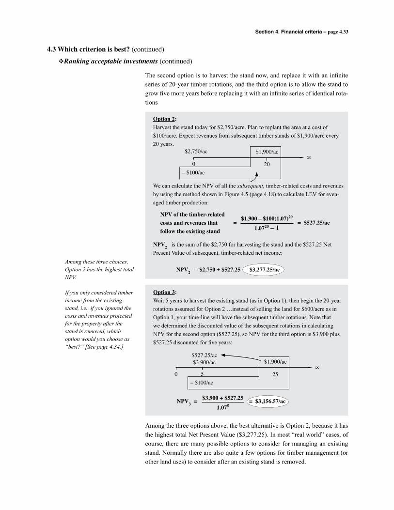
Section 4. Financial criteria – page 4.33
4.3 Which criterion is best? (continued)
vRanking acceptable investments (continued)
The second option is to harvest the stand now, and replace it with an infinite series of 20-year timber rotations, and the third option is to allow the stand to grow five more years before replacing it with an infinite series of identical rota-tions
Among these three choices, Option 2 has the highest total NPV.
If you only considered timber income from the existing stand, i.e., if you ignored the costs and revenues projected for the property after the stand is removed, which option would you choose as “best?” [See page 4.34.]
= = $527.25/ac$1,900 – $100(1.07)20
1.0720 – 1
0 20
$2,750/ac $1,900/ac 8
– $100/ac
NPV of the timber-related costs and revenues that follow the existing stand
Option 2:Harvest the stand today for $2,750/acre. Plan to replant the area at a cost of $100/acre. Expect revenues from subsequent timber stands of $1,900/acre every 20 years.
We can calculate the NPV of all the subsequent, timber-related costs and revenues by using the method shown in Figure 4.5 (page 4.18) to calculate LEV for even-aged timber production:
NPV2 is the sum of the $2,750 for harvesting the stand and the $527.25 Net Present Value of subsequent, timber-related net income:
NPV2 = $2,750 + $527.25 = $3,277.25/ac
NPV3 = = $3,156.57/ac$3,900 + $527.251.075
Option 3:Wait 5 years to harvest the existing stand (as in Option 1), then begin the 20-year rotations assumed for Option 2 …instead of selling the land for $600/acre as in Option 1, your time-line will have the subsequent timber rotations. Note that we determined the discounted value of the subsequent rotations in calculating NPV for the second option ($527.25), so NPV for the third option is $3,900 plus $527.25 discounted for five years:
5 25
$527.25/ac$3,900/ac $1,900/ac 8
– $100/ac0
Among the three options above, the best alternative is Option 2, because it has the highest total Net Present Value ($3,277.25). In most “real world” cases, of course, there are many possible options to consider for managing an existing stand. Normally there are also quite a few options for timber management (or other land uses) to consider after an existing stand is removed.
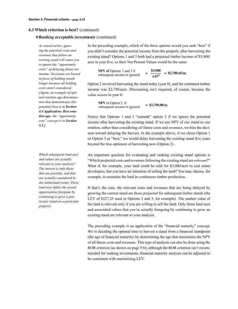
Section 4. Financial criteria – page 4.34
4.3 Which criterion is best? (continued)
vRanking acceptable investments (continued)
In the preceding example, which of the three options would you rank “best” if you didn’t consider the potential income from the property after harvesting the existing stand? Options 1 and 3 both had a projected timber income of $3,900/acre in year five, so their Net Present Values would be the same:
Option 2 involved harvesting the stand today (year 0), and the estimated timber income was $2,750/acre. Discounting isn’t required, of course, because the value occurs in year 0:
Notice that Options 1 and 3 “outrank” option 2 if we ignore the potential income after harvesting the existing stand. If we use NPV of one stand or one rotation, rather than considering all future costs and revenues, we bias the deci-sion toward delaying the harvest. In the example above, if we chose Option 1 or Option 3 as “best,” we would delay harvesting the existing stand five years beyond the true optimum of harvesting now (Option 2) .
An important question for evaluating and ranking existing stand options is “Which projected costs and revenues following the existing stand are relevant?” What if, for example, your land could be sold for $3,000/acre to real estate developers, but you have no intention of selling the land? You may choose, for example, to maintain the land in continuous timber production.
If that’s the case, the relevant costs and revenues that are being delayed by growing the current stand are those projected for subsequent timber stands (the LEV of $527.25 used in Options 2 and 3, for example). The market value of the land is relevant only if you are willing to sell the land. Only those land uses and associated values that you’re actually foregoing by continuing to grow an existing stand are relevant to your analysis.
The preceding example is an application of the “financial maturity” concept. We’re deciding the optimal time to harvest a stand from a financial standpoint (the age of financial maturity) by determining the age that maximizes the NPV of all future costs and revenues. This type of analysis can also be done using the ROR criterion (as shown on page 9.6); although the ROR criterion isn’t recom-mended for ranking investments, financial maturity analysis can be adjusted to be consistent with maximizing LEV.
Which subsequent land uses and values are actually relevant to your analysis? The answer is only those that are possible, and that are actually considered by the timberland owner. These land uses define the actual opportunities foregone by continuing to grow a par-ticular stand on a particular property.
NPV of Options 1 and 3 if subsequent income is ignored = = $2,780.65/ac
$3,9001.075
NPV of Option 2 if subsequent income is ignored = $2,750.00/ac
As stated earlier, ignor-ing the potential costs and revenues that follow an existing stand will cause you to ignore the “opportunity costs” of delaying future net income. Decisions are biased in favor of holding stands longer because all holding costs aren’t considered.[Again, an example of opti-mal rotation age determina-tion that demonstrates this potential bias is in Section4.4Application:Bestrota-tionage; the “opportunity cost” concept is in Section5.5.]
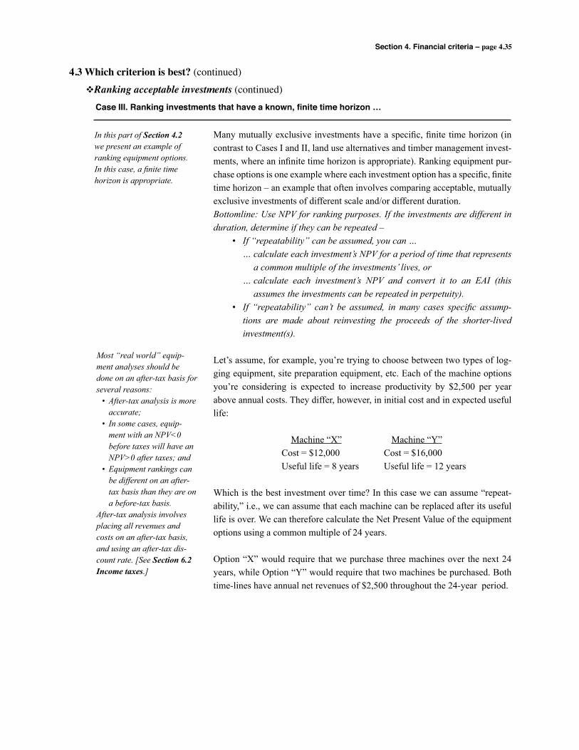
Section 4. Financial criteria – page 4.35
4.3 Which criterion is best? (continued)
vRanking acceptable investments (continued)
Many mutually exclusive investments have a specific, finite time horizon (in contrast to Cases I and II, land use alternatives and timber management invest-ments, where an infinite time horizon is appropriate). Ranking equipment pur-chase options is one example where each investment option has a specific, finite time horizon – an example that often involves comparing acceptable, mutually exclusive investments of different scale and/or different duration.Bottomline: Use NPV for ranking purposes. If the investments are different in duration, determine if they can be repeated – • If “repeatability” can be assumed, you can … … calculate each investment’s NPV for a period of time that represents
a common multiple of the investments’ lives, or … calculate each investment’s NPV and convert it to an EAI (this
assumes the investments can be repeated in perpetuity). • If “repeatability” can’t be assumed, in many cases specific assump-
tions are made about reinvesting the proceeds of the shorter-lived investment(s).
Let’s assume, for example, you’re trying to choose between two types of log-ging equipment, site preparation equipment, etc. Each of the machine options you’re considering is expected to increase productivity by $2,500 per year above annual costs. They differ, however, in initial cost and in expected useful life:
Machine “X” Machine “Y” Cost = $12,000 Cost = $16,000 Useful life = 8 years Useful life = 12 years
Which is the best investment over time? In this case we can assume “repeat-ability,” i.e., we can assume that each machine can be replaced after its useful life is over. We can therefore calculate the Net Present Value of the equipment options using a common multiple of 24 years.
Option “X” would require that we purchase three machines over the next 24 years, while Option “Y” would require that two machines be purchased. Both time-lines have annual net revenues of $2,500 throughout the 24-year period.
Most “real world” equip-ment analyses should be done on an after-tax basis for several reasons: • After-tax analysis is more
accurate; • In some cases, equip-
ment with an NPV<0 before taxes will have an NPV>0 after taxes; and
• Equipment rankings can be different on an after-tax basis than they are on a before-tax basis.
After-tax analysis involves placing all revenues and costs on an after-tax basis, and using an after-tax dis-count rate. [SeeSection6.2Incometaxes.]
In this part of Section4.2we present an example of ranking equipment options. In this case, a finite time horizon is appropriate.
Case III. Ranking investments that have a known, finite time horizon …
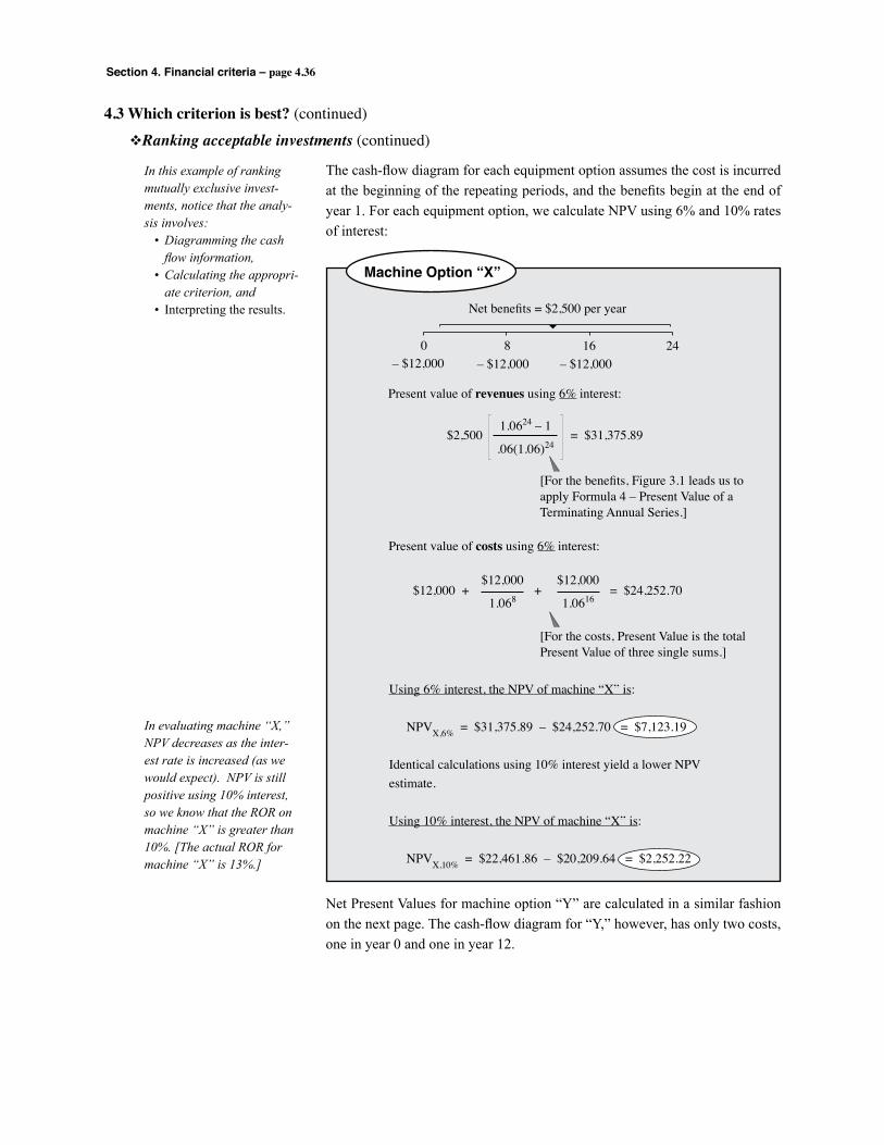
Section 4. Financial criteria – page 4.36
4.3 Which criterion is best? (continued)
vRanking acceptable investments (continued)
The cash-flow diagram for each equipment option assumes the cost is incurred at the beginning of the repeating periods, and the benefits begin at the end of year 1. For each equipment option, we calculate NPV using 6% and 10% rates of interest:
In this example of ranking mutually exclusive invest-ments, notice that the analy-sis involves: • Diagramming the cash
flow information, • Calculating the appropri-
ate criterion, and • Interpreting the results.
0 8 16 24– $12,000 – $12,000 – $12,000
Net benefits = $2,500 per year
Present value of revenues using 6% interest:
$2,500 = $31,375.891.0624 – 1
.06(1.06)24
[For the benefits, Figure 3.1 leads us to apply Formula 4 – Present Value of a Terminating Annual Series.]
Present value of costs using 6% interest:
$12,000 + + = $24,252.70$12,000
1.068
$12,000
1.0616
[For the costs, Present Value is the total Present Value of three single sums.]
Using 6% interest, the NPV of machine “X” is:
NPVX,6% = $31,375.89 – $24,252.70 = $7,123.19
Identical calculations using 10% interest yield a lower NPV estimate.
Using 10% interest, the NPV of machine “X” is:
NPVX,10% = $22,461.86 – $20,209.64 = $2,252.22
Machine Option “X”
Net Present Values for machine option “Y” are calculated in a similar fashion on the next page. The cash-flow diagram for “Y,” however, has only two costs, one in year 0 and one in year 12.
In evaluating machine “X,” NPV decreases as the inter-est rate is increased (as we would expect). NPV is still positive using 10% interest, so we know that the ROR on machine “X” is greater than 10%. [The actual ROR for machine “X” is 13%.]
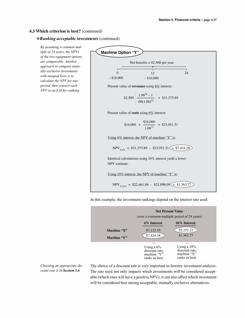
Section 4. Financial criteria – page 4.37
4.3 Which criterion is best? (continued)
vRanking acceptable investments (continued)
By assuming a common mul-tiple of 24 years, the NPVs of the two equipment options are comparable. Another approach to compare mutu-ally exclusive investments with unequal lives is to calculate the NPV for one period, then convert each NPV to an EAI for ranking.
Machine Option “Y”
0 12 24– $16,000 – $16,000
Net benefits = $2,500 per year
Present value of revenues using 6% interest:
$2,500 = $31,375.891.0624 – 1
.06(1.06)24
Present value of costs using 6% interest:
$16,000 + = $23,951.51$16,000
1.0612
Using 6% interest, the NPV of machine “Y” is:
NPVY,6% = $31,375.89 – $23,951.51 = $7,424.38
Identical calculations using 10% interest yield a lower NPV estimate.
Using 10% interest, the NPV of machine “Y” is:
NPVY,10% = $22,461.86 – $21,098.09 = $1,363.77
In this example, the investment rankings depend on the interest rate used:
Choosing an appropriate dis-count rate is in Section5.6.
Net Present Value(over a common-multiple period of 24 years)
Machine “X”
Machine “Y”
$7,123.19$7,424.38
6% Interest
$2,252.22$1,363.77
10% Interest
Using a 6%discount rate,machine “Y”ranks as best.
Using a 10%discount rate,machine “X”ranks as best.
The choice of a discount rate is very important in forestry investment analysis. The rate used not only impacts which investments will be considered accept-able (which ones will have a positive NPV); it can also affect which investment will be considered best among acceptable, mutually exclusive alternatives.
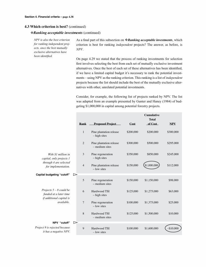
Section 4. Financial criteria – page 4.38
4.3 Which criterion is best? (continued)vRanking acceptable investments (continued)
As a final part of this subsection on vRankingacceptableinvestments, which criterion is best for ranking independent projects? The answer, as before, is NPV.
On page 4.29 we stated that the process of ranking investments for selection first involves selecting the best from each set of mutually exclusive investment alternatives. Once the best of each set of these alternatives has been identified, if we have a limited capital budget it’s necessary to rank the potential invest-ments – using NPV as the ranking criterion. This ranking is a list of independent projects because the list should include the best of the mutually exclusive alter-natives with other, unrelated potential investments.
Consider, for example, the following list of projects ranked by NPV. The list was adapted from an example presented by Gunter and Haney (1984) of bud-geting $1,000,000 in capital among potential forestry projects.
NPV is also the best criterion for ranking independent proj-ects, once the best mutually exclusive alternatives have been identified.
Cumulative Total Rank Proposed Project Cost of Cost NPV
1 Pine plantation release $200,000 $200,000 $300,000 – high sites
2 Pine plantation release $300,000 $500,000 $295,000 – medium sites
3 Pine regeneration $350,000 $850,000 $245,000 – high sites
4 Pine plantation release $150,000 $1,000,000 $112,000 – low sites
5 Pine regeneration $150,000 $1,150,000 $98,000 – medium sites
6 Hardwood TSI $125,000 $1,275,000 $63,000 – high sites
7 Pine regeneration $100,000 $1,375,000 $25,000 – low sites
8 Hardwood TSI $125,000 $1,500,000 $10,000 – medium sites
9 Hardwood TSI $100,000 $1,600,000 –$10,000 – low sites
Capital budgeting “cutoff”
NPV “cutoff”
With $1 million in capital, only projects 1 through 4 are selected
for implementation.
Projects 5 – 8 could be funded at a later time
if additional capital is available.
Project 9 is rejected because it has a negative NPV.
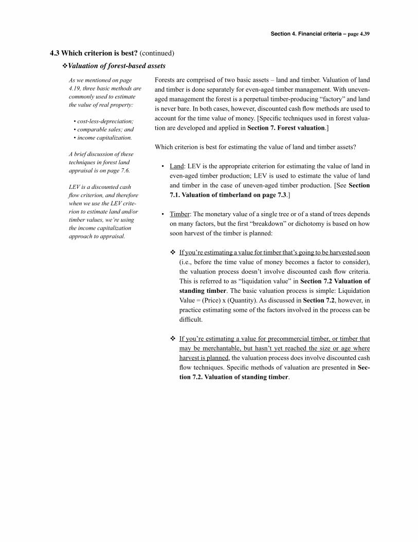
Section 4. Financial criteria – page 4.39
4.3 Which criterion is best? (continued)
vValuation of forest-based assets
Forests are comprised of two basic assets – land and timber. Valuation of land and timber is done separately for even-aged timber management. With uneven-aged management the forest is a perpetual timber-producing “factory” and land is never bare. In both cases, however, discounted cash flow methods are used to account for the time value of money. [Specific techniques used in forest valua-tion are developed and applied in Section 7. Forest valuation.]
Which criterion is best for estimating the value of land and timber assets?
• Land: LEV is the appropriate criterion for estimating the value of land in even-aged timber production; LEV is used to estimate the value of land and timber in the case of uneven-aged timber production. [See Section 7.1. Valuation of timberland on page 7.3.]
• Timber: The monetary value of a single tree or of a stand of trees depends on many factors, but the first “breakdown” or dichotomy is based on how soon harvest of the timber is planned:
v If you’re estimating a value for timber that’s going to be harvested soon (i.e., before the time value of money becomes a factor to consider), the valuation process doesn’t involve discounted cash flow criteria. This is referred to as “liquidation value” in Section 7.2 Valuation of standing timber. The basic valuation process is simple: Liquidation Value = (Price) x (Quantity). As discussed in Section 7.2, however, in practice estimating some of the factors involved in the process can be difficult.
v If you’re estimating a value for precommercial timber, or timber that may be merchantable, but hasn’t yet reached the size or age where harvest is planned, the valuation process does involve discounted cash flow techniques. Specific methods of valuation are presented in Sec-tion 7.2. Valuation of standing timber.
As we mentioned on page 4.19, three basic methods are commonly used to estimate the value of real property:
• cost-less-depreciation; • comparable sales; and • income capitalization.
A brief discussion of these techniques in forest land appraisal is on page 7.6.
LEV is a discounted cash flow criterion, and therefore when we use the LEV crite-rion to estimate land and/or timber values, we’re using the income capitalization approach to appraisal.
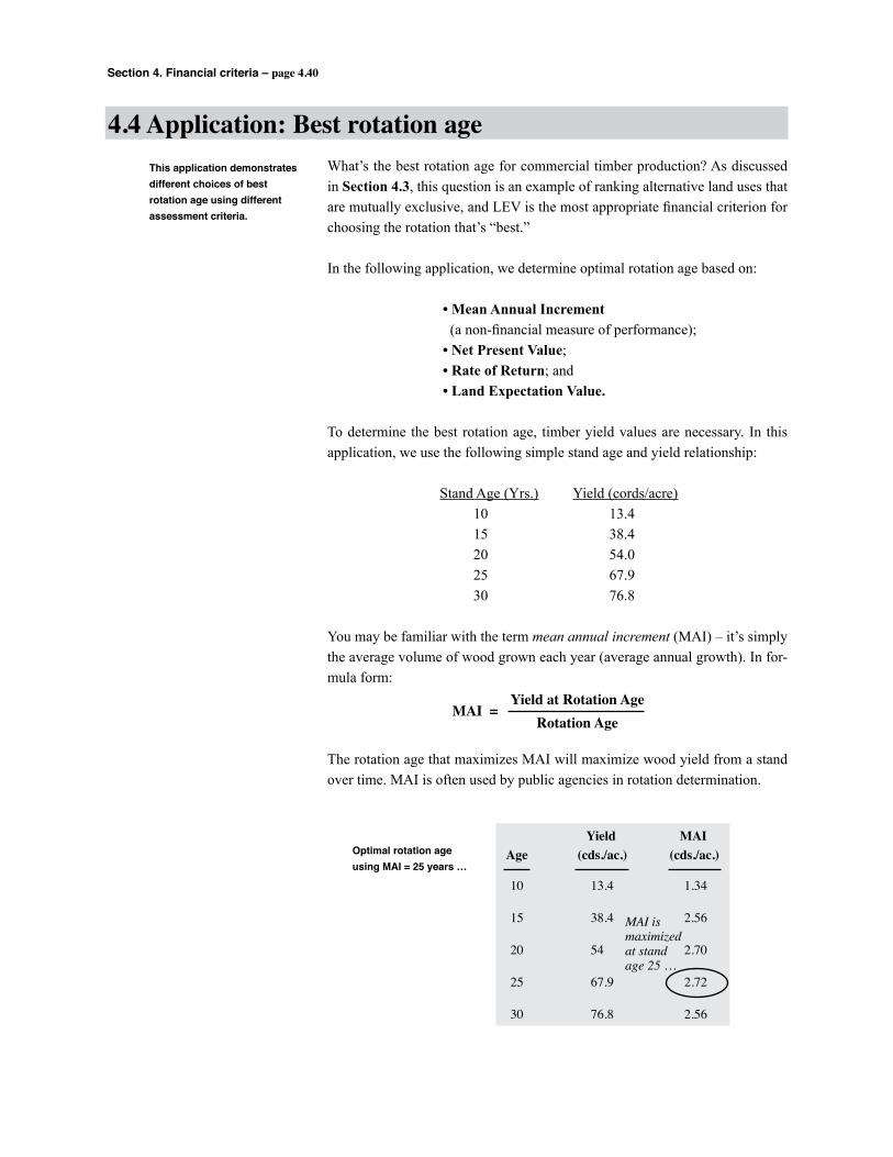
Section 4. Financial criteria – page 4.40
What’s the best rotation age for commercial timber production? As discussed in Section 4.3, this question is an example of ranking alternative land uses that are mutually exclusive, and LEV is the most appropriate financial criterion for choosing the rotation that’s “best.”
In the following application, we determine optimal rotation age based on:
• Mean Annual Increment (a non-financial measure of performance); • Net Present Value; • Rate of Return; and • Land Expectation Value.
To determine the best rotation age, timber yield values are necessary. In this application, we use the following simple stand age and yield relationship:
Stand Age (Yrs.) Yield (cords/acre) 10 13.4 15 38.4 20 54.0 25 67.9 30 76.8
You may be familiar with the term mean annual increment (MAI) – it’s simply the average volume of wood grown each year (average annual growth). In for-mula form:
The rotation age that maximizes MAI will maximize wood yield from a stand over time. MAI is often used by public agencies in rotation determination.
4.4 Application: Best rotation ageThis application demonstrates different choices of best rotation age using different assessment criteria.
MAI =Yield at Rotation Age
Rotation Age
Yield MAI Age (cds./ac.) (cds./ac.)
10 13.4 1.34 15 38.4 2.56 20 54 2.70
25 67.9 2.72
30 76.8 2.56
MAI ismaximizedat standage 25 …
Optimal rotation ageusing MAI = 25 years …
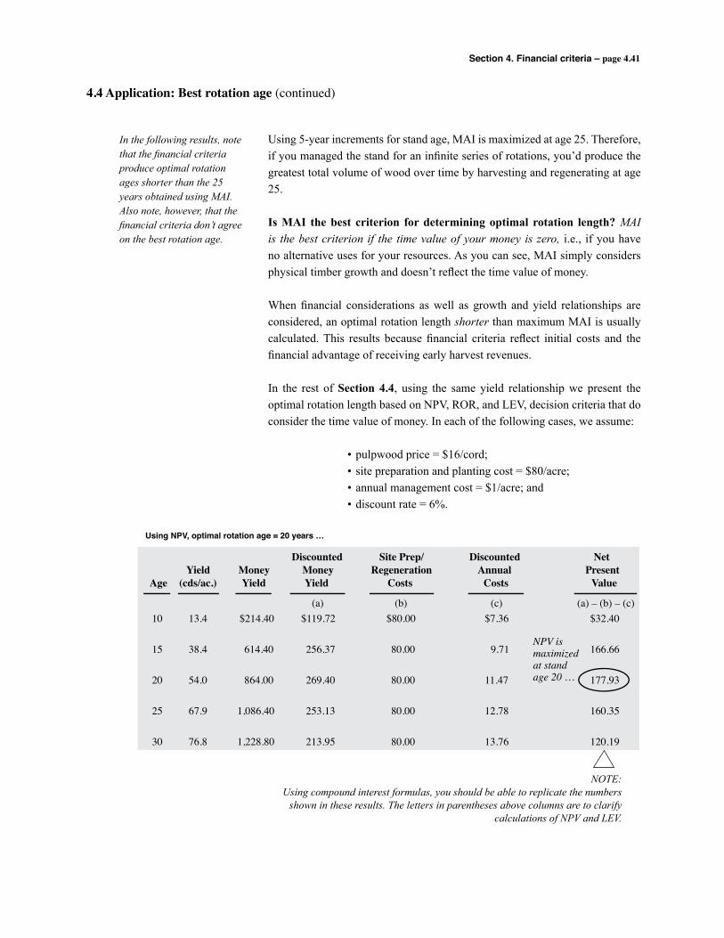
Section 4. Financial criteria – page 4.41
4.4 Application: Best rotation age (continued)
Using 5-year increments for stand age, MAI is maximized at age 25. Therefore, if you managed the stand for an infinite series of rotations, you’d produce the greatest total volume of wood over time by harvesting and regenerating at age 25.
Is MAI the best criterion for determining optimal rotation length? MAI is the best criterion if the time value of your money is zero, i.e., if you have no alternative uses for your resources. As you can see, MAI simply considers physical timber growth and doesn’t reflect the time value of money.
When financial considerations as well as growth and yield relationships are considered, an optimal rotation length shorter than maximum MAI is usually calculated. This results because financial criteria reflect initial costs and the financial advantage of receiving early harvest revenues.
In the rest of Section 4.4, using the same yield relationship we present the optimal rotation length based on NPV, ROR, and LEV, decision criteria that do consider the time value of money. In each of the following cases, we assume:
• pulpwood price = $16/cord; • site preparation and planting cost = $80/acre; • annual management cost = $1/acre; and • discount rate = 6%.
In the following results, note that the financial criteria produce optimal rotation ages shorter than the 25 years obtained using MAI. Also note, however, that the financial criteria don’t agree on the best rotation age.
Using NPV, optimal rotation age = 20 years …
Discounted Site Prep/ Discounted Net Yield Money Money Regeneration Annual Present Age (cds/ac.) Yield Yield Costs Costs Value
(a) (b) (c) (a) – (b) – (c) 10 13.4 $214.40 $119.72 $80.00 $7.36 $32.40
15 38.4 614.40 256.37 80.00 9.71 166.66
20 54.0 864.00 269.40 80.00 11.47 177.93
25 67.9 1,086.40 253.13 80.00 12.78 160.35
30 76.8 1,228.80 213.95 80.00 13.76 120.19
NPV ismaximizedat standage 20 …
NOTE: Using compound interest formulas, you should be able to replicate the numbers
shown in these results. The letters in parentheses above columns are to clarify calculations of NPV and LEV.
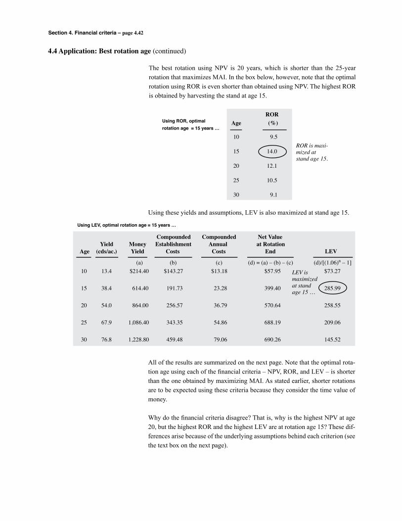
Section 4. Financial criteria – page 4.42
4.4 Application: Best rotation age (continued)
The best rotation using NPV is 20 years, which is shorter than the 25-year rotation that maximizes MAI. In the box below, however, note that the optimal rotation using ROR is even shorter than obtained using NPV. The highest ROR is obtained by harvesting the stand at age 15.
Using LEV, optimal rotation age = 15 years …
Compounded Compounded Net Value Yield Money Establishment Annual at Rotation Age (cds/ac.) Yield Costs Costs End LEV
(a) (b) (c) (d) = (a) – (b) – (c) (d)/[(1.06)n – 1] 10 13.4 $214.40 $143.27 $13.18 $57.95 $73.27
15 38.4 614.40 191.73 23.28 399.40 285.99
20 54.0 864.00 256.57 36.79 570.64 258.55
25 67.9 1,086.40 343.35 54.86 688.19 209.06
30 76.8 1,228.80 459.48 79.06 690.26 145.52
LEV ismaximizedat standage 15 …
ROR Age (%)
10 9.5 15 14.0 20 12.1
25 10.5
30 9.1
ROR is maxi-mized atstand age 15.
Using ROR, optimal rotation age = 15 years …
Using these yields and assumptions, LEV is also maximized at stand age 15.
All of the results are summarized on the next page. Note that the optimal rota-tion age using each of the financial criteria – NPV, ROR, and LEV – is shorter than the one obtained by maximizing MAI. As stated earlier, shorter rotations are to be expected using these criteria because they consider the time value of money.
Why do the financial criteria disagree? That is, why is the highest NPV at age 20, but the highest ROR and the highest LEV are at rotation age 15? These dif-ferences arise because of the underlying assumptions behind each criterion (see the text box on the next page).

Section 4. Financial criteria – page 4.43
4.4 Application: Best rotation age (continued)
Summary of optimal rotation results …
Net Yield MAI Present Age (cds/ac.) (cds/ac.) Value ROR (%) LEV
10 13.4 1.34 $32.40 9.5 $73.27
15 38.4 2.56 166.66 14.0 285.99
20 54.0 2.70 177.93 11.9 258.55
25 67.9 2.72 160.35 10.5 209.06
30 76.8 2.56 120.19 9.1 145.52
LEV ismaximizedat standage 15
ROR ismaximizedat standage 15NPV is
maximizedat standage 20MAI is
maximizedat standage 25
Each financial criterion reflects different man-agement objectives. The objective using NPV is to maximize the Net Present Value of the cash flows from one rotation. The objective using LEV is to maximize bare land value – the Net Present Value of all future rotations. The objective using ROR is to maximize the rate of return on the investment.
Why is there a difference between the optimal rotation ages using the financial criteria?
The differences arise because of the assumptions used for each criterion:
NPV … In the preceding application, NPV is the discounted net value of one rotation. Since only one stand of trees is considered, there is no incentive to harvest the stand so that the next stand can begin. The criterion ignores the opportunity cost of delay-ing subsequent timber revenues. Hence the optimal rotation is longer using this criterion than if subsequent stands are also considered in deciding rotation age.
LEV … LEV is the present value of net income from all future stands of timber. Recall from Section 4.3 that the criterion assumes an infinite series of rotations; the criterion therefore will result in a shorter optimal rotation than if only one stand is con-sidered. Because LEV considers all net income, it’s the most valid criterion for choosing the financially optimal rotation age.
ROR … ROR maximization simply produces the rotation that yields the greatest rate of return on the initial reforestation invest-ment. The criterion isn’t recommended for optimal rotation determination. In the application above, if the age increments had been one year rather than five years, the ROR criterion would have produced an optimal rotation age shorter than the LEV criterion.
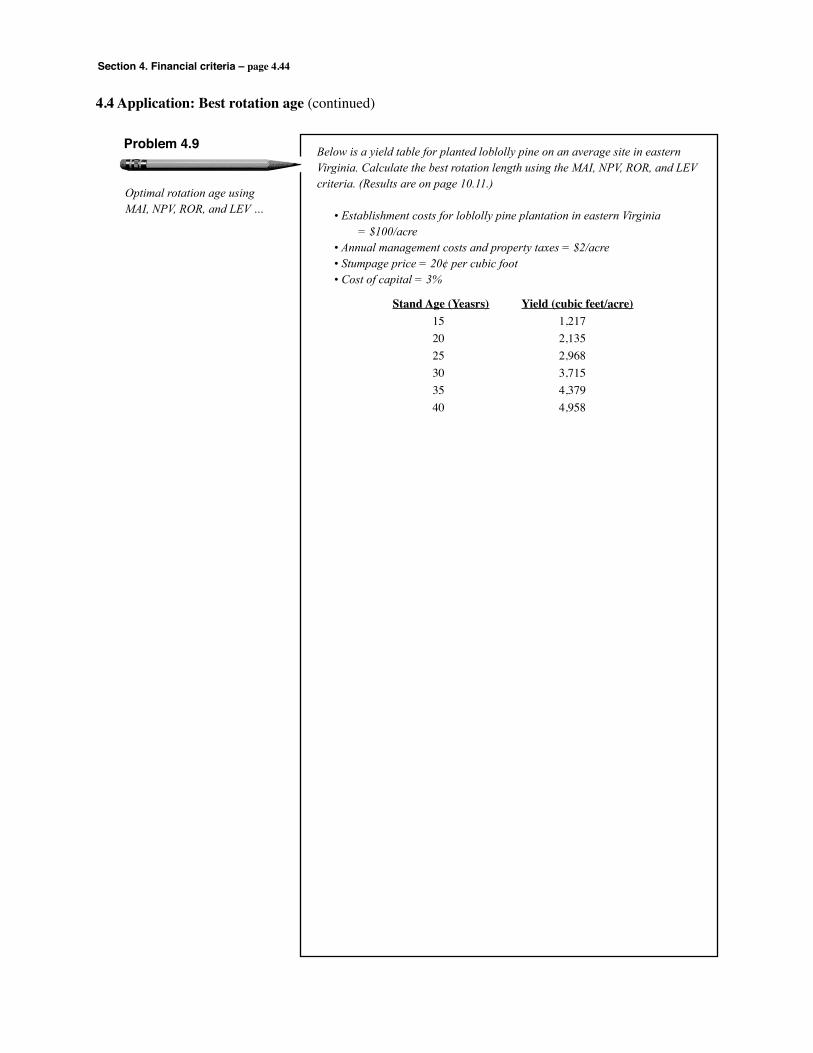
Section 4. Financial criteria – page 4.44
4.4 Application: Best rotation age (continued)
Optimal rotation age using MAI, NPV, ROR, and LEV …
Problem 4.9 Below is a yield table for planted loblolly pine on an average site in eastern Virginia. Calculate the best rotation length using the MAI, NPV, ROR, and LEV criteria. (Results are on page 10.11.)
• Establishment costs for loblolly pine plantation in eastern Virginia = $100/acre • Annual management costs and property taxes = $2/acre • Stumpage price = 20¢ per cubic foot • Cost of capital = 3%
Stand Age (Yeasrs) Yield (cubic feet/acre) 15 1,217 20 2,135 25 2,968 30 3,715 35 4,379 40 4,958
Section 4. Financial criteria – page 4.45
4.1 Introduction Seven “formal” financial criteria were presented in Section 4. They’re
“formal” because they’re calculated in a specific way – in most cases using compound interest formulas to account for the time value of money.
4.2 Financial criteria
vNetPresentValue NPV is the present value of all revenues for a project minus the present value
of all costs. If NPV is positive, a project is considered financially acceptable.
vEquivalentAnnualIncome EAI is NPV expressed on an “equivalent” annual basis. EAI is positive if
NPV is positive. In many cases EAI is calculated as information in addition to NPV; forest landowners, for example, can compare EAIs from timberland investments with potential annual income from other land uses like pasture or agricultural crops.
vBenefit/CostRatio The B/C ratio for a project is the present value of all revenues divided by the
present value of all costs. B/C indicates an investment’s net returns per dollar of expense. B/Cs are often used for financial analysis by U.S. government agencies.
vRateofReturn ROR is the rate of compound interest that’s earned on the funds invested in
a project. It’s the average rate of capital appreciation and is often called the “Return on Investment” (ROI). ROR is the interest rate that makes NPV = 0 and B/C = 1. If there are only two values associated with an investment – one cost and one revenue – ROR can be calculated exactly using a simple formula (Formula 11 in Figure 3.1). If a project has more than two values, however, ROR must be estimated through a systematic (or “iterative”) process.
�ROR is a very popular criterion because it’s readily understood and applied. A project is considered financially acceptable if the ROR is greater than the best rate that can be earned on other investments of equal risk, duration, and liquid-ity. If you’re evaluating whether a specific project is acceptable, ROR will yield results consistent with other financial criteria. ROR isn’t recommended, however, for ranking projects that are all acceptable.
4.5 Review of Section 4
Section 4. Financial criteria

Section 4. Financial criteria – page 4.46
4.5 Review of Section 4 (continued)
4.2 Financial criteria (continued)
vCompositeRateofReturn The “composite” or “realizable” rate of return was introduced in Section 4.
The criterion isn’t universally accepted as a valid investment analysis tool, however. It was included in Section 4 because some computer programs for forestry investment analysis report the criterion.
vPaybackPeriod This is simply the length of time it takes for an investment to “pay back” its
initial costs. The criterion doesn’t account for the time value of money, and therefore wasn’t included in Section 4.3 Which criterion is best?
vLandExpectationValue LEV is an estimate of the value of bare land for growing timber in perpetuity.
It’s the Net Present Value of all revenues and costs associated with growing timber on a tract of land. LEV is thus a special case of NPV; it’s NPV where all present and future costs and revenues expected from a tract of land are considered (hence the name Land Expectation Value).
LEV is calculated by estimating all costs and revenues for the first rotation of timber, compounding these to the end of the first rotation, and assuming the net value will be repeated as a perpetual periodic series. LEV therefore assumes a perpetual series of rotations that are identical biologically and eco-nomically, i.e., from the standpoint of timber yields as well as from the stand-point of economic variables such as timber prices and the costs of production.
LEV is affected by site quality, costs, prices, yields, management regime and rotation age, the interest rate, and other factors. The EAI associated with an LEV is calculated by multiplying the LEV by the interest rate:
EAI associated with an LEV = LEV (i)
Section 4. Financial criteria – page 4.47
4.5 Review of Section 4 (continued)
4.3 Which criterion is best?
The “best” criterion depends on the objective of the analysis. Discounted cash flow techniques and financial criteria can be used for :
vAccept/rejectinvestmentdecisions; vRankingacceptableinvestments; and vValuationofforest-basedassets.
vAccept/rejectinvestmentdecisions For accept/reject decisions, the compound interest-based financial criteria
– NPV, EAI, B/C, and ROR – will yield the same yes or no answer. That is, if a specific project is financially attractive based on NPV, it will also be acceptable based on EAI, B/C, and/or ROR. These criteria won’t disagree on whether a specific investment is acceptable.
vRankingacceptableinvestments If the purpose of your analysis is to choose among investment options, all of
which are financially acceptable, NPV is recommended. EAI and LEV are specialized forms of NPV that have specific uses in investment ranking. In Section 4.3, three important cases of forestry investment rankings were dis-cussed:
Case I. Ranking land use alternatives… The bottomline for choosing land use alternatives is to use the NPV of all
future costs and revenues. In some cases this NPV is the LEV criterion. With land use alternatives of different duration, NPV (or LEV) can be expressed as an EAI.
Case II. Ranking forest management methods and regimes… Deciding which set of cultural practices is best, and which management
combination of thinning regime, rotation length, etc., is best from a finan-cial standpoint is the same as ranking and choosing the best land use alternative. The bottomline is therefore the same one stated in Case I for ranking land use alternatives.
Case III. Ranking investments that have a known, finite time horizon… Choosing between types of equipment is an example of this kind of invest-
ment ranking. The bottomline is to use NPV for ranking purposes. If the investments are different in duration, determine if “repeatability” can be assumed. If the investments can be repeated to a common multiple, NPV can be used for ranking.
In some cases, the best choice among mutually exclusive alternative invest-ments must be made, and then capital must be budgeted among competing independent projects. For this purpose, NPV is recommended.
Section 4. Financial criteria – page 4.48
4.5 Review of Section 4 (continued)
4.3 Which criterion is best? (continued)
vValuationofforest-basedassets The third broad use for financial criteria is in estimating monetary values for
land and/or timber. If you’re estimating a value for land, LEV is the appro-priate criterio; this is discussed in Section 7.2 Valuation of timberland. If you’re estimating the monetary value of timber, discounted cash flow methods may or may not be necessary, depending on how soon the timber will be har-vested; this is discussed in Section 7.3 Valuation of standing timber.
4.4 Application: Best rotation age This Section includes an example application of determining optimal rotation
age for a loblolly pine stand. LEV is recommended for this purpose, and the application demonstrates that other criteria can disagree with LEV on which rotation age is best.
4.6 Additional references
Some of the references we list in Section 4 are grouped, and for convenience they’re placed near the related discussion. In Section 4 these groups include:
ROR-related references General … Some general ROR references are on page 4.11
Composite ROR references … References that relate to the composite rate of return criterion are on page 4.16.
Reinvestment … Some references that relate to whether ROR calculations include a reinvestment assumption are on page 4.27.
ROR for ranking … ROR isn’t recommended for ranking investments. References that relate to this topic are on page 4.28.
Section 4. Financial criteria – page 4.49
4.6 Additional references (continued)
Additional references in Section 4, and others that relate to financial criteria and their application in forestry include:
Bullard, S.H., T.A. Monaghan and T.J. Straka. 1986. Introduction to forest valuation and investment analysis (VI. Decision Criteria, p.35). Public. 1546, Miss. Coop. Ext. Serv., Miss. State Univ., Mississippi State, MS, 131p.
Clutter, J.L., J.C. Fortson, L.V. Pienaar, G.H. Brister and R.L. Bailey. 1983. Timber Management: A Quantita-tive Approach (Chapter 5, Section 5.2 Criteria for Financial Investments). John Wiley & Sons, New York, 333p.
Davis, L.S. and K.N. Johnson. 1987. Forest Management (Part 2, Chapter 8. Evaluation of Project and Planning Alternatives). McGraw-Hill, New York, 790p.
Duerr, W.A. 1993. Introduction to Forest Resource Economics (Part III. Genetic Production). McGraw-Hill, New York, 485p.
Fortson, J.C. 1972. Which criterion? Effect of choice of the criterion on forest management plans. For. Sci. 18:292–297.
Foster, B.B. 1982. Economic nonsense. (Letter to the Editor on the Composite Rate of Return) J. For. 80(9):566.
Foster, B.B. and G.N. Brooks. 1983. Rates of return: Internal or composite? (see Harpole, 1984) J. For. 81(10):669–670.
Foster, B.B. 1984. A service forester’s guide to investment terminologies – which ones are most easily understood by landowners? South. J. Appl. For. 8(3):115–119.
Gansner, D.A. and D.W. Larsen. 1969. Pitfalls of using internal rate of return to rank investments in forestry. Res. Note NE–106, USDA For. Serv., Northeast. For. Exper. Stn., Upper Darby, PA, 5p.
Gunter, J.E. and H.L. Haney, Jr. 1984. Essentials of Forestry Investment Analysis (Decision Criteria, p. 57). Copy-right Gunter–Haney, 337 p.
Hansen, B.G. and A.J. Martin. 1983. That nonsensical composite internal rate. (Letter to the Editor on the Com-posite Rate of Return) J. For. 81(7):422.
Harpole, G.B. 1984. “Rates of return: Internal or composite?” – A response. (see Foster and Brooks, 1983) J. For. 82(9):558, 559.
Leuschner, W.A. 1984. Introduction to Forest Resource Management (Part I, Chapter 5. Decision Criteria). John Wiley & Sons, New York, 298p.
Klemperer, W.D. 1979. Inflation and present value of timber income after taxes. J. For. 77:94–96.
Section 4. Financial criteria – page 4.50
4.6 Additional references (continued)
Klemperer, W.D. 1981a. Interpreting the realizable rate of return. (see Schallau and Wirth, 1981 and Klemperer, 1981b) J. For. 79(9):616–617.
Klemperer, W.D. 1981b. Realizable rate of return: A rejoinder. (see Schallau and Wirth, 1981 and Klemperer, 1981a) J. For. 79(10):673.
Klemperer, W.D. 1987. Possible misinterpretations of equivalent annual incomes in inflationary times. North. J. Appl. For. 4:210–211.
Klemperer, W.D. 1996. Forest Resource Economics and Finance (Chapter 4. The Forest as Capital). McGraw-Hill, New York, 551p.
Marty, R.J. 1969. The composite internal rate of return. For. Sci. 16:276–279.
Mills, T.J. and G.E. Dixon. 1982. Ranking independent timber investments by alternative investment criteria. Res. Pap. PSW–166, USDA For. Serv., Pac. Southwest For. and Range Exper. Stn., Berkeley, CA, 8p.
Schallau, C.H. and M.E. Wirth. 1980. Reinvestment rate and the analysis of forestry enterprises. J. For. 78(12):740–742.
Schallau, C.H. and M.E. Wirth. 1981. Interpreting the realizable rate of return: A reply. (see Klemperer, 1981a and 1981b) J. For. 79(9):618.
Smith, H.C. and J.B. Corgel. 1992. Real Estate Perspectives. An Introduction to Real Estate. Irwin, Homewood, IL, 747p.
Uys, H.J.E. 1990a. Financial decision criteria and real price changes. S. African For. J. 154:15–17.
Uys, H.J.E. 1990b. A new form of internal rate of return. S. African For. J. 154:24–26.
Section 5. Financial analysis concepts – page 5.1
Section
5 Financialanalysis concepts
5.1 Introduction 5.15.2 Marginal analysis 5.25.3 Sunk costs 5.35.4 Risk and uncertainty 5.45.5 Opportunity costs 5.115.6 Choosing a discount rate 5.145.7 Review of Section 5 5.19
“If you would know the value of money, go and try to borrow some.”– Benjamin Franklin
The Way to Wealth (1757)
Accurate project analysis and assessment involves correct use of the formulas in Section 3, and correct calculation and application of the financial criteria in Sec-tion 4. More issues are often involved, however, than simply using the financial information for a project in a way that’s “mechanically” correct.
How do you choose a discount rate? How do you “handle” the opportunity cost of land in forestry investment analysis? These and other important questions arise in many applications of financial criteria to forestry decision making. We’ve grouped some of the most important topics in applied analysis here in Section 5. Taxes and inflation are also extremely important in forestry investment analysis, and they are the subject of Section 6.
5.1 Introduction
Page
Section 5 includes concepts that are basic to many finan-cial analyses in forestry.
1. Basics of compound interest
2. Four basic formulas
3. Twelve formulas
4. Financial criteria
5. Financial analysis concepts
6. Inflation and taxes
7. Forest valuation
8. An example computer program
9. Review for the Registered
Forester exam
10. Solutions to problems
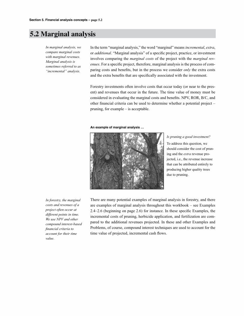
Section 5. Financial analysis concepts – page 5.2
In marginal analysis, we compare marginal costs with marginal revenues. Marginal analysis is sometimes referred to as “incremental” analysis.
In forestry, the marginal costs and revenues of a project often occur at different points in time. We use NPV and other compound interest-based financial criteria to account for their time value.
In the term “marginal analysis,” the word “marginal” means incremental, extra, or additional. “Marginal analysis” of a specific project, practice, or investment involves comparing the marginal costs of the project with the marginal rev-enues. For a specific project, therefore, marginal analysis is the process of com-paring costs and benefits, but in the process we consider only the extra costs and the extra benefits that are specifically associated with the investment.
Forestry investments often involve costs that occur today (or near to the pres-ent) and revenues that occur in the future. The time value of money must be considered in evaluating the marginal costs and benefits. NPV, ROR, B/C, and other financial criteria can be used to determine whether a potential project – pruning, for example – is acceptable.
There are many potential examples of marginal analysis in forestry, and there are examples of marginal analysis throughout this workbook – see Examples 2.4–2.6 (beginning on page 2.6) for instance. In these specific Examples, the incremental costs of pruning, herbicide application, and fertilization are com-pared to the additional revenues projected. In these and other Examples and Problems, of course, compound interest techniques are used to account for the time value of projected, incremental cash flows.
5.2 Marginal analysis
An example of marginal analysis …
Is pruning a good investment?
To address this question, we should consider the cost of prun-ing and the extra revenue pro-jected, i.e., the revenue increase that can be attributed entirely to producing higher quality trees due to pruning.
Section 5. Financial analysis concepts – page 5.3
Costs incurred in the past cannot be changed and are therefore not relevant to today’s analyses and decisions.
Costs incurred in the past are “sunk.” They cannot be changed and are outside the realm of current decisions. Sunk costs should therefore not be included in calculating NPV, B/C, or other financial criteria, unless the analysis is histori-cal in context.
The past costs of an asset are irrelevant to decisions about the future. The cur-rent value of the property, equipment, or other asset may be relevant, and that value is affected by the asset’s attributes or condition, but the price paid for the asset in the past is irrelevant (again, unless you’re calculating a historical rate of return, for example).
An example of sunk costs …
Last year you spent $125/acre for site preparation and tree planting. You’re now considering the need for a herbicide application that will increase seedling sur-vival and growth .
The $125/acre you’ve already spent cannot be changed and therefore isn’t rel-evant to your herbicide decision. In calculating a marginal ROR or NPV for the herbicide investment, the planting cost should be ignored.
What is relevant to the herbicide analysis?The physical characteristics of the site and current biological opportunities for tree release are highly relevant to your analysis and decision; you now have an asset that has attributes that are directly related to the site preparation and tree and planting that took place in the past. The actual expenses incurred to achieve the attributes of your stand, however, cannot be changed and are irrelevant to current decisions.
Another example of sunk costs …
You recently spent $2,500 to replace a vehicle’s engine, and now you’re trying to decide if you should invest in additional repairs.
This is another example of marginal analysis – you’re weighing the added costs against the added benefits of specific, additional repairs. In this case, the $2,500 has been “sunk” into the vehicle recently, but this amount is irrelevant.
What is relevant to the decision on further repairs?The fact that the vehicle has a new engine is relevant to the decision on further repairs. The marginal benefit of the repairs is probably much higher because the vehicle has enhanced value. The marginal cost of further repairs is not affected by the engine’s cost, however, so the actual cost incurred in the past isn’t a factor in the marginal analysis.
5.3 Sunk costs
Seedling establishment costs should be considered “sunk” if they have already been incurred.
Just as in the reforestation example above, the current condition of an equip-ment asset is relevant, but what it cost in the past to achieve that condition is irrelevant.
Section 5. Financial analysis concepts – page 5.4
“Forestry economics concerns choices, and these exist only in the future; the past is a closed book.” This quote from Duerr (1993) fits well with the “sunk cost” discussion on the previous page, but it also fits well with the concepts of risk and uncertainty. In forest valuation and investment analysis, choices “exist only in the future,” yet we are uncertain about important factors in the future such as timber yields and prices.
Is there a difference between risk and uncertainty? According to Lueschner (1984), risk exists if a probability distribution can be attributed to various out-comes of a decision, and uncertainty exists if there is no information about their probabilities. Various methods have been proposed to adjust for risk and uncertainty in forestry decision making. These techniques include calculating “certainty equivalents” for various outcomes (Clutter et al. 1983), and adjusting the discount rate for risk (Foster 1979).
Rather than summarizing all potential approaches to accounting for risk and uncertainty, we devote Section 5.4 to a basic discussion and an applied example of “sensitivity analysis” as a practical means of evaluating important assump-tions that are necessary because we aren’t certain of future costs, revenues, and other analysis inputs. We conclude with references on the broader topics of risk and uncertainty in financial analysis in forestry. Section 5.4 therefore has three subsections:
vBasic concepts in sensitivity analysis; vAn example sensitivity analysis; and vReferences on risk and uncertainty.
Our simple financial analyses thus far have assumed we know the value of key variables such as management costs, stumpage prices, yields, length of rotation, and interest rate. Of course, in many analyses several of the values may not be known with certainty, and reasonable assumptions must be made.
When you perform a financial analysis, prudence requires that you evaluate how “sensitive” your results are to the many assumptions in the model. In most applications, there is no need for calculus or sophisticated mathematical analy-sis. Simply modifying the key variables, one at a time, will easily demonstrate how important each assumed value is to the NPV, ROR, or other financial crite-rion you’ve calculated; this systematic process is termed “sensitivity analysis.”
Section 5.4 includes a basic discussion of sensitivity anal-ysis as a means of evaluating important assumptions in forest valuation and invest-ment analysis. Important references on various tech-niques for dealing with risk and uncertainty are included on page 5.9.
vBasic concepts in sensitivity analysis
5.4 Risk and uncertainty
Sensitivity analysis is an orderly or systematic process of varying key assumptions in an analysis, and evaluat-ing their impact on financial criteria and decisions.
Section 5. Financial analysis concepts – page 5.5
5.4 Risk and uncertainty (continued)
vBasic concepts in sensitivity analysis (continued)
There are at least two analysis situations where you definitely should assess the sensitivity of your results to potential changes in the values that were used:
• If you’re highly uncertain of the exact value(s) of one or more key variables in the analysis (the following discussion helps identify which variables may be critical); or
• If the value you calculated for NPV, B/C, etc., is marginal in accept-ability (for example, if NPV is near zero, B/C is near one, etc.). In such cases, the accept/reject decision for the investment may be “sensitive” to changes in key values in the analysis.
The potential influence of major variables can be seen in a simple NPV cal-culation. Considering only the front-end costs of reforestation and the income obtained from a single future yield, for example, the NPV of one timber rotation is:
This relation merely says that the NPV of a reforestation investment is the discounted harvest value minus the cost of site preparation and planting. Our simple example includes the four major variables that affect the economics of reforestation … i, n, HV, and RC.
The interest rate, “i,” is one of the most important variables affecting forestry decisions. When compounding or discounting over a rotation of many years, a small change in the interest rate can make a great difference in an investment’s NPV, B/C, etc.
The choice of an appropriate interest rate is therefore a key decision affecting forestry investment analysis. A very important concept is that if the interest vari-able changes, through a change in time preference (how soon you need cash), market rates, or landownership, forestry investment decisions may change dra-matically. See Example 7.3 (page 7.9) for an example of how dramatically the discount rate can affect timberland value estimates. Section 5.6 Choosing a discount rate has more information on this important topic.
NPV = – RCHV
(1 + i)n
Where HV = Harvest Value (in year n) RC = Reforestation Cost (in year 0), and n = rotation length in years.
If the interest rate changes, forestry investment decisions may change dramatically.
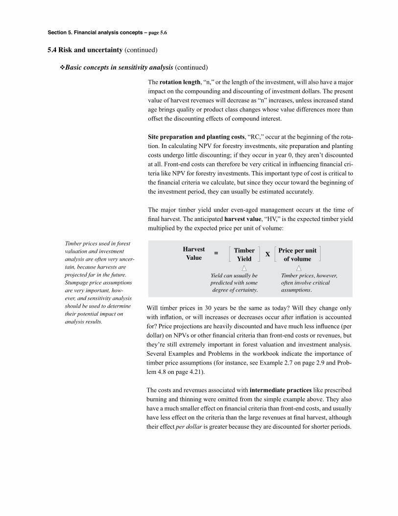
Section 5. Financial analysis concepts – page 5.6
5.4 Risk and uncertainty (continued)
vBasic concepts in sensitivity analysis (continued)
The rotation length, “n,” or the length of the investment, will also have a major impact on the compounding and discounting of investment dollars. The present value of harvest revenues will decrease as “n” increases, unless increased stand age brings quality or product class changes whose value differences more than offset the discounting effects of compound interest.
Site preparation and planting costs, “RC,” occur at the beginning of the rota-tion. In calculating NPV for forestry investments, site preparation and planting costs undergo little discounting; if they occur in year 0, they aren’t discounted at all. Front-end costs can therefore be very critical in influencing financial cri-teria like NPV for forestry investments. This important type of cost is critical to the financial criteria we calculate, but since they occur toward the beginning of the investment period, they can usually be estimated accurately.
The major timber yield under even-aged management occurs at the time of final harvest. The anticipated harvest value, “HV,” is the expected timber yield multiplied by the expected price per unit of volume:
Timber prices used in forest valuation and investment analysis are often very uncer-tain, because harvests are projected far in the future. Stumpage price assumptions are very important, how-ever, and sensitivity analysis should be used to determine their potential impact on analysis results.
Yield can usually be predicted with some degree of certainty.
Timber prices, however, often involve critical assumptions.
HarvestValue
= Price per unitof volume
TimberYield
X
Will timber prices in 30 years be the same as today? Will they change only with inflation, or will increases or decreases occur after inflation is accounted for? Price projections are heavily discounted and have much less influence (per dollar) on NPVs or other financial criteria than front-end costs or revenues, but they’re still extremely important in forest valuation and investment analysis. Several Examples and Problems in the workbook indicate the importance of timber price assumptions (for instance, see Example 2.7 on page 2.9 and Prob-lem 4.8 on page 4.21).
The costs and revenues associated with intermediate practices like prescribed burning and thinning were omitted from the simple example above. They also have a much smaller effect on financial criteria than front-end costs, and usually have less effect on the criteria than the large revenues at final harvest, although their effect per dollar is greater because they are discounted for shorter periods.

Section 5. Financial analysis concepts – page 5.7
5.4 Risk and uncertainty (continued)
vAn example sensitivity analysis
How sensitive is NPV to changes or possible errors in each of the four major variables we’ve discussed – i, n, HV, and RC? A simple example illustrates their potential influence.
Assume a 25-year rotation of slash pine. The regeneration cost is $100/acre and the harvest yield is 40 cords/acre. Pulpwood is worth $15/cord and the interest rate is 4%. The NPV of one rotation is:
What if “i” changes?Assume a 10% change in the interest rate, a change that in absolute terms appears to be trivial – 3.6% and 4.4% appear to be very close to 4%. Look at the impact of this 10% change on NPV, however:
Using an interest rate of … … 3.6%, NPV = $147.83/acre (an increase of 18.2%). … 4.4%, NPV = $104.47/acre (a decrease of 16.5%).
Again, the example simply demonstrates that even relatively small changes in “i” can result in significant changes in the financial criteria upon which long-term forestry investment decisions are based.
What if “n” changes?The length of the investment period (in this case the rotation length) is also an extremely important factor in a financial analysis. As discussed in Section 1 (page 1.10), the basic compound interest relationship is exponential, and the exponent in the relationship is the length of the period.
In our slash pine example, if the rotation period is increased or decreased by 10% (and if we simplify by assuming the same timber volume and value is obtained), the impact on NPV is significant:
Using a rotation length of … … 22.5 years, NPV = $148.26/acre (an increase of 18.5%). … 27.5 years, NPV = $104.05 (a decrease of 16.8%).
Under the assumption that “all else is equal,” our NPV result is quite sensitive to the length of the rotation.
The discount rate and the assumed rate of real price increase are critical factors in forestry NPV calculations. Relatively small changes can have relatively great impacts on NPV, B/C and other finan-cial criteria.
NPV = – $100 = $125.07/acre$600
(1.04)25
Section 5. Financial analysis concepts – page 5.8
What’s the impact of an error in “RC?”The effect of a change in reforestation costs on our example is easy to see. These costs occur in year 0 and are subtracted directly from the present value of revenues to obtain NPV. There, if RC increases by $1, NPV decreases by $1, etc. [As part of your reforestation effort, herbicides are applied in year two to help ensure seedling survival. Would a $1 increase in the cost of this “RC” activity also have a $1 impact on NPV?]
What if “HV” changes?Harvest values are subject to discounting, and a $1 change in HV therefore has less than a $1 impact on NPV. In this example, a $1 change in final harvest value in year 25 impacts NPV by:
$1/(1.04)25 = $0.3751, or about 38¢
The example clearly demonstrates that accuracy in reforestation and other front-end costs is much more important on a per dollar basis than final harvest values. With longer rotations, of course, harvest value changes will have less impact on a per dollar basis.
This is not to say, however, that changes in HV are not important. Because final harvest values are typically relatively large in absolute terms, errors of more than a few percentage points may significantly impact NPV. Consider our example assuming a 2%/year increase in prices. Rather than $15/cord, pro-jected price for the harvest in year 25 is:
$15 (1.02)25 = $24.61/cord.
This means the projected HV is $24.61 x 40 = $984.36/acre, and the estimated NPV is:
Our NPV estimate more than doubled because we incorporated a 2% annual rate of increase in prices. Real price increases are often assumed in forest valu-ation and investment analysis. As shown in this example, these assumptions can have a very dramatic impact on analysis results.
5.4 Risk and uncertainty (continued)
vAn example sensitivity analysis (continued)
Front-end costs like site preparation and planting are very important in NPV results. They’re near the present, however, and can usually be estimated accu-rately.
NPV = – $100 = $269.25/acre$984.36(1.04)25
As stated on page 5.6, timber price assumptions are often very uncertain, because harvests are projected far in the future. They are very important, however. Sensitiv-ity analysis should be used to determine the impact of price assumptions in most forest valuation and investment analysis problems.

Section 5. Financial analysis concepts – page 5.9
5.4 Risk and uncertainty (continued)
vRisk and uncertainty references
These articles and reports include discussions of methods to account for risk and uncertainty in forest valuation and investment analysis …
Baumgartner, D.C. and C.A. Hyldahl. 1991. Using price data to consider risk in the evaluation of forest man-agement investments. Gen. Tech. Rep. NC–144, USDA For. Serv., North Cent. For. Exper. Stn., St. Paul, MN, 8p.
Casasempere, A. 2004. Planning, appraisal and risk analysis in clonal forestry projects. Plantation Forest Bio-technology for the 21st century. 2004:363-375.
Caulfield, J.P., E. Shoulders and B.G. Lockaby. 1989. Risk-efficient species-site selection decisions for south-ern pines. Can. J. For. Res. 19(6):743–753.
Chang, S.J. 1980. Discounting under risk: Comments on adjusting discount rates (see Foster, 1979, 1980). J. For. 78:634,635.
Clutter, J.L., J.C. Fortson, L.V. Pienaar, G.H. Brister and R.L. Bailey. 1983. Timber Management: A Quantita-tive Approach (Chapter 6, Section 6.3 Methods for Evaluating Risk in Forestry Investments). John Wiley & Sons, New York, 333p.
Duerr, W.A. 1993. Introduction to Forest Resource Economics. McGraw-Hill, New York, 485p.
Gunter, J.E. and H.L. Haney, Jr. 1984. Essentials of Forestry Investment Analysis (Incorporating Risk in the Analysis, p. 134). Copyright Gunter–Haney, 337 p.
Engelhard, R.J. and W.C. Anderson. 1983. A method of assessing risk in forestry investments. Res. Pap. SO–189, USDA For. Serv., South. For. Exper. Stn., New Orleans, LA, 13p.
Flora, D.F. 1964. Uncertainty in forestry investment decisions. J. For. 62(6):376–379.
Foster, B.B. 1979. Adjusting discount rates for risk. J. For. 77:287–288.
Foster, B.B. 1980. Rebuttal (see Chang, 1980 and Foster, 1979). J. For. 78:636.
Hyldahl, C.A. and D.C. Baumgartner. 1991. Risk analysis and timber investments: A bibliography of theory and applications. Gen. Tech. Rep. NC–143, USDA For. Serv., North Cent. For. Exper. Stn., St. Paul, MN, 29p.
Klemperer, W.D. 1996. Forest Resource Economics and Finance. McGraw-Hill, New York, 551p.
Klemperer, W.D. and J.F. Cathcart. 1990. Estimating discount rate adjustments for forest investment risk. Proc., XIX IUFRO World Congress, Montreal, Canada, 4:113–115.
Section 5. Financial analysis concepts – page 5.10
5.4 Risk and uncertainty (continued)
vRisk and uncertainty references (continued)
Leuschner, W.A. 1984. Introduction to Forest Resource Management (Part I, Chapter 9. Adjusting for Risk). John Wiley & Sons, New York, 298p.
Liley, B. 2000. Focus on the treatment of risk in forest valuations. New Zealand J. For. 45(2):3–12.
Marty, R.J. 1964. Analyzing uncertain timber investments. Res. Pap. NE-23, USDA For. Serv. Northeast. For. Exper. Stn., Broomall, PA, 21p.
McKillop, D.G. and R.W. Hutchinson. 1990. The determination of risk-adjusted discount rates for private sector forestry investment. Forestry (Oxford) 63(1):29–38.
Pukkala, T. 1998. Multiple risks in multi-objective forest planning: Integration and importance. For. Ecol. Man. 111(2-3):265–284.
Pukkala, T. and Kangas, J. 1996. A method for integrating risk and attitude toward risk into forest planning. For. Sci. 42(2):198–205.
Thomson, T.A. 1989. Evaluating some financial uncertainties of tree improvement using the capital asset pric-ing model and dominance analysis. Can. J. For. Res. 19(11):1380–1388.
Section 5. Financial analysis concepts – page 5.11
Economic resources have value because they can be used to produce goods and services. When an economic resource is put to a particular use, it competes with alternative uses. This means the price bid for a resource must be at least as much as the resource’s value in the alternative use. This alternative use is commonly called an “opportunity cost” – it represents opportunities (revenues or other benefits) foregone.
n A simple illustration is a miser who has $1,000 in cash. The local bank pays 4% on savings accounts, but instead of using the bank the miser stores the money under his mattress for a year. For the year, the miser is foregoing the opportunity to earn : (.04)($1,000) = $40.00. The $40 is the opportunity cost of hoarding the $1,000 rather than investing it in a savings account.
n If you pay $450 cash for a rifle or shotgun, use the gun for six years, and then sell it for $450, would your six years of use be free? The use was free only if you had no alternative uses for those funds – in such a case, your “alternative rate of return” would be 0%. If you do have alternatives (and most of us do), then there is an opportunity cost associated with owning the gun. If a bank would pay you 3%, for example, you could have earned (.03)($450) = $13.50 each year.
There are many examples of opportunity costs in forest valuation and invest-ment analysis. A very important example is the opportunity cost of forest land. we can’t grow timber without tying up significant areas of land, and that land has monetary value. The remainder of Section 5.5 demonstrates the importance and proper inclusion of land value in an investment analysis.
First consider an example forestry NPV calculation without including the value of the land in the analysis:
What’s the NPV/acre for growing timber under the following assumptions? Year 0, Site prep and planting cost = $160/acre Year 16, Thinning income = 5 cds./ac. at $19.50/cd. = $97.50/acre Year 22, Thinning income = 8 cds./ac. at $19.50/cd. = $156.00/acre Year 27, Final harvest = 66 cds/ac. at $19.50 = $1,287.00/acre Years 1–27, Annual costs = $2.50/acre Alternative rate of return = 4%
The present value of the two costs is $200.82, and the present value of the three revenues is $564.25. So NPV = $363.43/acre if we don’t include the opportunity cost of land
Opportunity costs are revenues or other benefits foregone because you decide to use land, capital or other resources in a specific way.
5.5 Opportunity costs
If you borrow money, it obviously isn’t “free;” you pay interest for the right to use it. Neither is it “free” to use your own funds or other resources like land; by using resources in one way you forego opportunities to earn interest or to benefit from other uses and potential investments.
NPV without land value in the calculation …
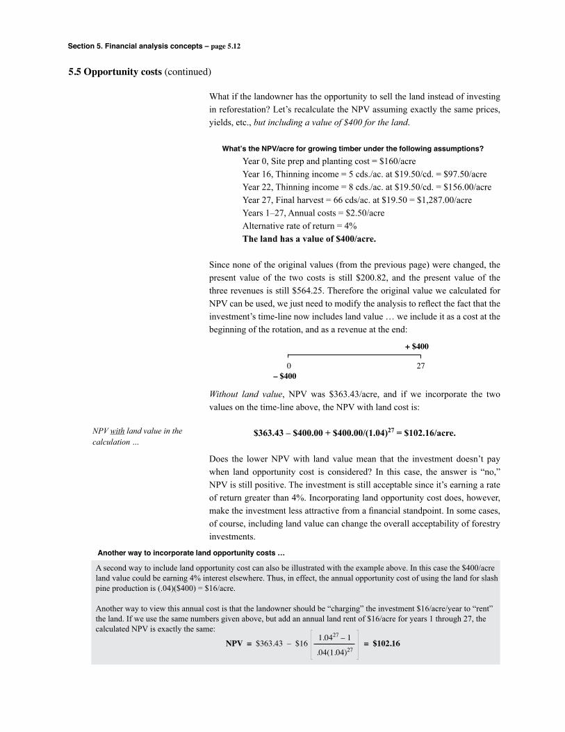
Section 5. Financial analysis concepts – page 5.12
5.5 Opportunity costs (continued)
What if the landowner has the opportunity to sell the land instead of investing in reforestation? Let’s recalculate the NPV assuming exactly the same prices, yields, etc., but including a value of $400 for the land.
What’s the NPV/acre for growing timber under the following assumptions? Year 0, Site prep and planting cost = $160/acre Year 16, Thinning income = 5 cds./ac. at $19.50/cd. = $97.50/acre Year 22, Thinning income = 8 cds./ac. at $19.50/cd. = $156.00/acre Year 27, Final harvest = 66 cds/ac. at $19.50 = $1,287.00/acre Years 1–27, Annual costs = $2.50/acre Alternative rate of return = 4% The land has a value of $400/acre.
Since none of the original values (from the previous page) were changed, the present value of the two costs is still $200.82, and the present value of the three revenues is still $564.25. Therefore the original value we calculated for NPV can be used, we just need to modify the analysis to reflect the fact that the investment’s time-line now includes land value … we include it as a cost at the beginning of the rotation, and as a revenue at the end:
Without land value, NPV was $363.43/acre, and if we incorporate the two values on the time-line above, the NPV with land cost is:
$363.43 – $400.00 + $400.00/(1.04)27 = $102.16/acre.
Does the lower NPV with land value mean that the investment doesn’t pay when land opportunity cost is considered? In this case, the answer is “no,” NPV is still positive. The investment is still acceptable since it’s earning a rate of return greater than 4%. Incorporating land opportunity cost does, however, make the investment less attractive from a financial standpoint. In some cases, of course, including land value can change the overall acceptability of forestry investments.
NPV with land value in the calculation …
0 27
+ $400
– $400
A second way to include land opportunity cost can also be illustrated with the example above. In this case the $400/acre land value could be earning 4% interest elsewhere. Thus, in effect, the annual opportunity cost of using the land for slash pine production is (.04)($400) = $16/acre.
Another way to view this annual cost is that the landowner should be “charging” the investment $16/acre/year to “rent” the land. If we use the same numbers given above, but add an annual land rent of $16/acre for years 1 through 27, the calculated NPV is exactly the same:
Another way to incorporate land opportunity costs …
NPV = $363.43 – $16 = $102.161.0427 – 1
.04(1.04)27

Section 5. Financial analysis concepts – page 5.13
5.5 Opportunity costs (continued)
An interesting case where land cost is often omitted is in estimating the value of a precommercial stand of timber. In such valuation problems, if land costs are omitted from the analysis, precommercial timber will be undervalued (see page 7.16 “Valuation of immature timber”). Another case where the opportu-nity cost of land is very important in forestry is financial maturity analysis (see page 9.6).
When should the opportunity cost of land be included in forest valuation and investment analysis? If timberland or the capital invested in timberland has alternative uses, potential income from the best use should be included as a production cost in investment analyses. This is the case in precommercial stand valuation, and in timber financial maturity analysis.
What land cost do you use? That is, what “value” is appropriate? This is deter-mined by the actual alternative uses for the property. If the landowner would consider selling the land, the market value in the land’s “highest and best” use is appropriate. If the landowner doesn’t intend to sell the land, opportunity costs are defined by other uses. For example, if a property has an existing stand of timber, growing future rotations of timber is an opportunity that can’t be real-ized until the existing stand is harvested. The landowner incurs an opportunity cost of (LEV)(i) each year the current stand is maintained.
Land cost isn’t included in LEV calculations because the purpose of the cal-culation is to estimate the value of the land if it’s used for timber production. Land opportunity cost also isn’t a factor in most examples of marginal analysis. If you’re evaluating the marginal costs and benefits of fertilization or other stand treatments, for example, only the additional costs and revenues specifi-cally associated with the activity are relevant.
When should the opportunity cost of land be included, and what value is appropriate?
LEV is the appropriate land value if the land will be maintained in perpetual timber production.

Section 5. Financial analysis concepts – page 5.14
In the previous subsection, we defined “opportunity costs” as revenues or other benefits foregone because you decide to use land, capital, or other resources in a specific way. A discount rate is a compound rate of interest that reflects the opportunity cost of capital for an individual, a firm, a government agency, etc.
Different names are frequently used to indicate the discount rate: • Cost of capital. This name simply reflects the interest rate as a mea-
sure of the opportunity cost of capital – the rate you could have earned on capital in other uses, or the rate you’re paying others to use their funds.
• Guiding rate of return. The discount rate is sometimes referred to as a “guiding rate” because the rate is used as a yardstick – a guide for evaluating the acceptability and attractiveness of different invest-ments.
• Hurdle rate. Much like the “guiding rate,” the name “hurdle rate” simply indicates that the discount rate can be a specific hurdle; invest-ments that don’t yield a specified minimum rate don’t make it over the hurdle of acceptability.
• Alternative rate of return. As stated with the “cost of capital” discus-sion, the discount rate sometimes indicates other opportunities (alter-natives) for using capital. To be comparable, an “alternative rate of return” should be for investments of comparable duration, risk, and liquidity.
In addition to the above terms, sometimes the phrase “exception rate” is used to indicate discount rates applied to investments in timber and timberland. If a specific use of capital provides benefits that aren’t reflected by its projected cash flows, an exception may be made in the rate of return that’s considered acceptable; in most cases, this means a lower rate of return is used.
For example, a forest products corporation may use a guiding rate of return defined by the corporation’s cost of capital (see the next page); but the corpo-ration may make an exception for timber-related investments. They may, for example, view timber as a strategic asset – control over raw material supply may be a part of their corporate strategy – but these strategic benefits aren’t reflected in timber’s projected cash flows. In such cases, a lower rate of return, or “exception rate,” is used.
“All approaches to obtaining an interest rate come back to the same concept – opportu-nity cost.”(Thompson 1976)
5.6 Choosing a discount rate
In some cases, an “exception rate” is used to guide invest-ment decisions in forestry; an exception is made by some landowners, for example, because they consider timber production to be a strategic investment.
vNames for the discount rate
Although different terms are used for the discount rate, they all indicate the compound rate of interest that reflects the time value of money at a given time and place, for a specific individ-ual, corporation, government agency, etc.

Section 5. Financial analysis concepts – page 5.15
The appropriate rate of interest to use in forest valuation and investment analy-sis usually depends on who owns the land or other resource:
• Public agencies Discount rates for public agencies are often specified by law. The fed-
eral government, for example, requires that agencies use a “real” (unin-flated) rate of 10% unless a special rate, formula or other guideline is set by law – basically an “exception rate” as discussed on the previous page.
The USDA Forest Service currently uses a “real” rate of 4% for long-term investments (generally more than 10 years), and 10% for other, shorter-term investments. For further information, see the article by Row, Kaiser, and Sessions, and the USDA Forest Service Economic Analysis Manual references in the vDiscount rate references subsec-tion (page 5.17).
• Corporations Privately-owned as well as publicly-held corporations usually define
discount rates as a weighted average cost of capital – the cost of debt capital and the cost of equity capital weighted by the firms’s percentage of debt and equity. For example, a firm with a debt:equity ratio of 60:40 that is paying 8% interest on debt capital and 15% on equity capital has a weighted average cost of capital of: .60(.08) + .40(.14) = .104 = 10.4%.
As stated on the previous page, forest products corporations sometimes specify an “exception rate” for timber-related investments that “fit in” with overall corporate strategic goals for self-sufficiency in timber supply.
• Private individuals Individuals may specify their discount rate by considering alternative
uses for their capital; alternative rates may thus be the rate they expect to earn on their investments, or they may be the rates they are paying on borrowed capital. Each private individual is different, however, and discussion may be needed to elicit an individual landowner’s prefer-ences for money today versus money in the future. A survey of over 800 private landowners in Mississippi reported hurdle rates (inflated terms and before taxes) of 8% for 5-year forestry investments, and 11% for 15-year and 13% for 30-year forestry investments (Bullard et al. 2002). The survey was done in 2000, when bank savings accounts were earning 4-5%, and Certificates of Deposit were earning over 6%.
5.6 Choosing a discount rate (continued)
Discount rates specified for a specific forest valuation or investment analysis problem should be consistent in terms of inflation, and for private firms and individuals they should also be consistent in terms of taxes. This is mentioned briefly on the following page; Section 6. Taxes and inflation has examples of accounting for taxes and inflation in defining a discount rate.
vDiscount rates for different landowners
Section 5. Financial analysis concepts – page 5.16
Because of their importance in investment analysis, inflation and taxes are discussed in Section 6. It should be noted here, however, that it is extremely important in specifying a discount rate that the rate be consistent with other aspects of the analysis in terms of taxes and inflation.
There are four options for the discount rate to use in forest valuation and invest-ment analysis, depending on whether or not inflation and taxes are considered:
Terms like “nominal” and “real” and techniques for determining after tax dis-count rates and other values are discussed in Section 6.
5.6 Choosing a discount rate (continued)
The discount rate should be consistent with other aspects of the analysis. If all values are without inflation and are before taxes, for example, the discount rate should be a real, before-tax rate of interest.
vDiscount rates for different landowners
Nominal, After-taxDiscount Rate
Nominal, Before-taxDiscount Rate
Real, After-taxDiscount Rate
Real, Before-taxDiscount Rate
Considering Taxes Not Considering Taxes
With Inflation
Excluding Inflation
Section 5. Financial analysis concepts – page 5.17
5.6 Choosing a discount rate (continued)
Anderson, W.C., R.W. Guldin and J.M. Vasievich. 1983. Assessing risk to plantation investments from insect attacks. Res. Pap. SO–231, USDA For. Serv., South. For. Exper. Stn., New Orleans, LA, 6p.
Baumol, W.J. 1968. On the social rate of discount. Amer. Econ. Rev., Sept., pp. 788–802.
Binkley, C.S. 1981. Duration-dependent discounting. Can. J. For. Res. 11:454–456.
Bullard, S.H., J.E. Gunter, M.L. Doolittle and K.G. Arano. 2002. Discount rates for nonindustrial private forest landowners in Mississippi: How high a hurdle? South. J. Appl. For. 26(1):26-31.
Duerr, W.A. 1993. Introduction to Forest Resource Economics (Chapter 20, Finding a Guiding Rate of Return). McGraw-Hill, 485p.
Fitzsimons J. 1986. Discount rates and forestry decisions. New Zealand For. 31(2):22–25.
Fortson, J.C. 1986. Factors affecting the discount rate for forestry investments. For. Prod. J. 36:67–72.
Foster, B.B. 1979. Multiple discount rates for evaluating public forestry investments. For. Chron. 55:17–19.
Gunter, J.E. and H.L. Haney, Jr. 1984. Essentials of Forestry Investment Analysis (Estimating Cost of Capital, p. 125). Copyright Gunter–Haney, 337 p.
Guttenberg, S. 1950. The rate of interest in forest management. J. For. 48:3–7.
Hanke, S.H and J.B. Anwyll. 1980. On the discount rate controversy. Public Policy 28(2):171–183.
Hannesson, R. 1987. The effect of the discount rate on the optimal exploitation of renewable resources. Marine Resour. Econ. 4(4):319–329.
Harou, P.A. 1985. On a social discount rate for forestry (see Price, 1987 and Harou, 1987a). Can. J. For. Res. 15:927–934.
Harou, P.A. 1987a. On a social discount rate for forestry: Reply. (see Harou, 1985 and Price, 1987) Can. J. For. Res. 17:1473.
Harou, P.A. 1987b. Discount rate for appraising multiple use forestry projects. In Proc. 18th IUFRO World Congress for Economic Value Analysis of Multiple Use Forestry, H.F. Kaiser and P. Brown eds., Oregon State Univ., Corvallis, OR, pp.137–149.
Kronrad, G.D. and J.E. de Steiguer. 1983. Relationships between discount rates and investment lengths among nonindustrial private landowners. Res. Note Series No. 19, Small Woodlot R&D Program, N.C. State Univ., Raleigh, NC, 19p.
Kula, E. 1988. Future generations: the modified discounting method. Project Appraisal. 3(2):85–8
vDiscount rate references

Section 5. Financial analysis concepts – page 5.18
5.6 Choosing a discount rate (continued)
Manning, G. 1977. Evaluating public forestry investments in British Columbia: The choice of discount rate. For. Chron. 53:155–158.
Markandya, A. and D. Pearce. 1988. Natural environments and the social rate of discount. Project Appraisal 3(1):2–12.
O’Toole, R. 1986. Investing in timber lands. Forest Watch: The Citizen’s Forestry Magazine 7:15–18 (Includes a discussion of USDA Forest Service discount rates.)
Price, C. 1973. To the future: With indifference or concern? – the social discount rate and its implications in land use. J. Agric. Ec. 24:393–398.
Price, C. 1987. On a social discount rate for forestry: Comment (see Harou, 1985, 1987a). Can. J. For. Res. 17:1472, 1473.
Price, C. and Nair, C.T.S. 1985. Social discounting and the distribution of project benefits. J. Dev. Stud. 21(4):25–32.
Quirk, J. and K. Terasawa. 1991. Choosing a government discount rate, an alternative approach. J. Envir. Econ. and Management, January, pp. 16–28.
Row, C., H.F. Kaiser and J. Sessions. 1981. Discount rate for long-term Forest Service investments. J. For.
79(6):367–376.
Seagraves, J.A. 1970. More on the social rate of discount. Quar. J. Econ. 84(3):430–450.
Shepard, W. 1925. The bogey of compound interest. J. For. 29:251–259. Thompson, E.F. 1976. Analyzing forestry investments. In: Economics of Southern Forest Resources Manage-
ment. 25th Annual Forestry Symposium, Louisiana State Univ. Div. Of Cont. Educ. pp. 67–83.
Tillman, D.A. 1985. Forest Products: Advanced Technologies and Economic Analyses. (Chapter 3. The Dis-count Rate for Current Forest Industry Investments) Academic Press, Inc., New York, 283p.
USDA Forest Service. (1984 draft). Economic and social analysis handbook. FSH 1909.17.
Zinkhan, F.C. 1988. Forestry projects, modern portfolio theory, and discount rate selection. South. J. Appl. For. 12:132–135
[Note that articles concerned with adjusting discount rates for risk are included under the vRisk and uncer-tainty references subsection on pages 5.9-5.10.]
vDiscount rate references (continued)

Section 5. Financial analysis concepts – page 5.19
5.1 Introduction Section 5 includes basic concepts that are important in many forest valua-
tion and investment analysis problems. Marginal analysis concepts, choosing a discount rate, and correctly handling sunk costs, opportunity costs, and risk are critical for effective analysis. Not understanding these concepts can result in a “fatal error” in the analysis; including sunk costs in a marginal analysis, for example, will completely invalidate the results (and may seriously damage the credibility of the analyst).
5.2 Marginal analysis In a marginal analysis, we compare a project’s marginal costs with its mar-
ginal revenues. In this context, the word “marginal” means additional, extra, or incremental; marginal analysis is sometimes referred to as “incremental analysis.” Many of the examples and problems in this workbook are examples of marginal analysis. When we calculate an NPV associated with silvicultural treatments like fertilization, herbicide application, etc., we’re comparing the marginal costs and the marginal revenues of the treatment. We use compound interest formulas to account for the time value of the marginal costs and rev-enues in calculating financial criteria like NPV and ROR.
5.3 Sunk costs The past costs associated with an investment are “sunk” and cannot be changed
with decisions today. Sunk costs are therefore irrelevant in most types of investment analysis, including marginal analysis. One example of when sunk costs should be considered is where the analysis is historical in context. For example, calculating the ROR of a forestry investment over its full time span will involve past costs as well as projected costs and revenues.
5.4 Risk and uncertainty Several methods can be used to account for the risk and uncertainty inherent
in forest valuation and investment analysis. We include references to these methods in Section 5.4, but we discuss only one method – sensitivity analysis – using a simple example of pine plantation costs and revenues for demon-stration. In forest valuation and investment analysis, front-end costs like site preparation and planting are very important. They’re near the present, how-ever, and can usually be estimated accurately. Timber price assumptions, how-ever, are often very uncertain, simply because in many cases timber harvests are projected far in the future. Sensitivity analysis should be used to assess the impact of different timber price assumptions on analysis results.
5.7 Review of Section 5
Section 5. Financial analysis concepts

Section 5. Financial analysis concepts – page 5.20
5.7 Review of Section 5 (continued)
5.5 Opportunity costs Opportunity costs are revenues or other benefits foregone because you decide
to use land, capital, or other assets in a specific way. If you use land to pro-duce timber, for example, you’re foregoing potential revenues from other uses of the land (or from the capital invested in the land). If timberland or the capital invested in timberland has alternative uses, income from the best alternative use should be included as a production cost in valuation and/or investment analysis. This is the case in precommercial stand valuation (dis-cussed in Section 7), and in timber financial maturity analysis. The land value to use is LEV if the land will be maintained in timber production; market value should be used if the landowner would consider selling the land.
5.6 Choosing a discount rate The discount rate is sometimes referred to as the cost of capital, the guiding
rate of return, the hurdle rate, and the alternative rate of return. The appropri-ate rate to use in forest valuation and investment analysis depends on who owns the land or other resources involved:
• Public agencies. The appropriate rate for public agencies is often speci-fied by law. The USDA Forest Service uses 4% for long-term invest-ments (generally more than 10 years), and 10% for other, shorter-term investments.
• Corporations. The time value of money for corporations is typically defined as a weighted average cost of debt and equity capital. Corpora-tions sometimes use an “exception” rate for timber-related investments, however, because timber production promotes corporate strategic goals for timber supply.
• Private individuals. Private landowners often specify their discount rate by considering alternative uses for their capital – rates they expect to earn on similar investments, for example, or rates they’re paying on borrowed capital. Current wealth is a very important factor in determin-ing the time value of money for private individuals.
Regardless of the type of ownership involved, the discount rate used to address a specific forest valuation or investment analysis question should be consistent in terms of taxes and inflation. For example, if all costs and rev-enues are without inflation and before taxes, the discount rate should be a real, before-tax rate of interest.

Section 6. Inflation and taxes – page 6.1
“The difference between a taxidermist and a tax collector is that thetaxidermist will only take your hide.”
– Mark Twain (attributed)
The most important aspect of accounting for inflation in forest valuation and investment analysis is consistency – either include inflation in the discount rate and in all costs and revenues, or leave it out entirely. If you’re consistent, whether you include or exclude inflation won’t impact the outcome of your analysis unless the investment has costs that are “capitalized” for tax purposes (such costs are described in Section 6.2. Income taxes). If capitalized costs are involved, inflation should be included in the discount rate and in all costs and revenues.
6.1 Inflation
Inflation and taxes are considered in a separate Section to emphasize their importance, and to allow the basic concepts and issues to be discussed in an appro-priate level of detail.
Section
6 Inflation and taxes
6.1 Inflation 6.16.2 Income taxes 6.106.3 Review of Section 6 6.26
Page
1. Basics of compound interest
2. Four basic formulas
3. Twelve formulas
4. Financial criteria
5. Financial analysis concepts
6. Inflation and taxes
7. Forest valuation
8. An example computer program
9. Review for the Registered
Forester exam
10. Solutions to problems
Section 6. Inflation and taxes – page 6.2
Since forestry investments typically involve dollar values that occur years in the future, it’s extremely important to treat inflation consistently. We stress the need for consistency because examples of inconsistency in forestry project analysis are relatively common, and because they can have a very negative impact on the attractiveness of forest-related investments.
Two examples of inconsistency in accounting for inflation: n It’s inconsistent to use an inflated interest rate to discount uninflated
dollar values. This error occurs, for example, when an interest rate that includes inflation is used to discount future timber sale revenues that are obtained by multiplying future timber volumes by the prices that prevail today (uninflated values).
n It’s inconsistent to calculate a forestry project’s ROR without consid-ering inflation, and then compare the ROR with an alternative rate of interest that does include inflation. Comparing an uninflated ROR for a forestry investment with the interest rate paid by a bank, for example, is inappropriate since the bank rate includes inflation – you expect the bank to pay the rate quoted for your account regardless of the rate of inflation that occurs.
Again, “consistency” means that inflation should either be included or excluded from all values in an analysis. If inflation is included in an analysis, the costs, revenues, and discount rate are referred to as nominal or in current dollar terms. If inflation is excluded they’re said to be in real or constant dollar terms.
As an example of inflation’s influence on future values, consider how a general rise in prices affects the value of a specific product like timber. If a general rise in prices causes timber that’s valued at $1,000 today to be valued at $1,090 after one year (an increase of 9%), how much will the timber be worth after two years, assuming the same rate of general price increase, and assuming the same timber volume and quality?
Since the general price increase (inflation) occurs in each of the two years pro-jected, the estimated timber value in two years is:
$1,000 (1.09)2 = $1,188.10 after the second year.
If the timber also increased in value by 5% in real terms, that is, over and above inflation, its value after two years would be:
$1,000 (1.09)2 (1.05)2 = $1,309.88.
“Real” means inflation is omitted. A “real price increase,” for example, is over and above infla-tion. An analysis that’s done “in real terms” is one where inflation is not included in the costs, the revenues, and the discount rate.
6.1 Inflation (continued)
vAccounting for inflation (continued)
In general, what impact do these example incon-sistencies have on the attractiveness of timber related investments?
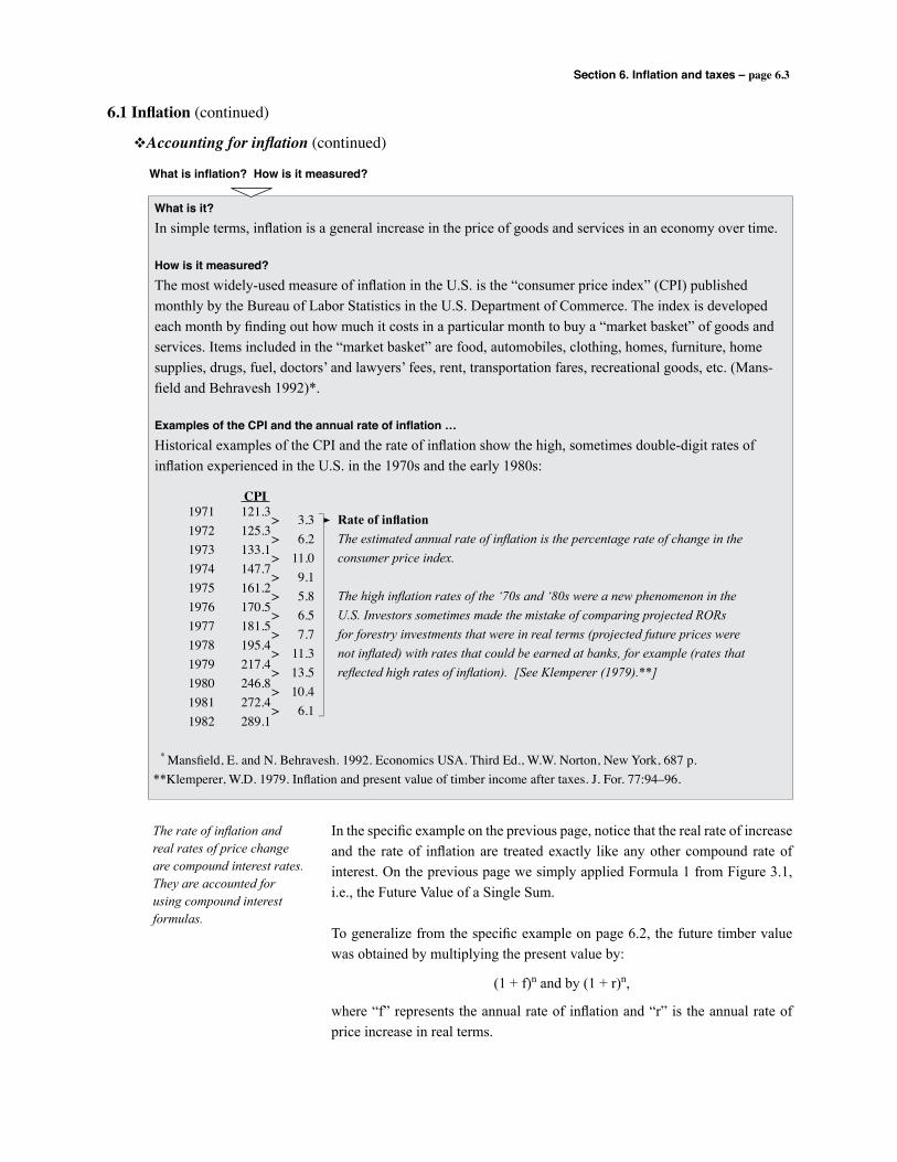
Section 6. Inflation and taxes – page 6.3
What is it?In simple terms, inflation is a general increase in the price of goods and services in an economy over time.
How is it measured?The most widely-used measure of inflation in the U.S. is the “consumer price index” (CPI) published monthly by the Bureau of Labor Statistics in the U.S. Department of Commerce. The index is developed each month by finding out how much it costs in a particular month to buy a “market basket” of goods and services. Items included in the “market basket” are food, automobiles, clothing, homes, furniture, home supplies, drugs, fuel, doctors’ and lawyers’ fees, rent, transportation fares, recreational goods, etc. (Mans-field and Behravesh 1992)*.
Examples of the CPI and the annual rate of inflation …Historical examples of the CPI and the rate of inflation show the high, sometimes double-digit rates of inflation experienced in the U.S. in the 1970s and the early 1980s:
The rate of inflation and real rates of price change are compound interest rates. They are accounted for using compound interest formulas.
6.1 Inflation (continued)
vAccounting for inflation (continued)
Rate of inflationThe estimated annual rate of inflation is the percentage rate of change in the consumer price index.
The high inflation rates of the ‘70s and ‘80s were a new phenomenon in the U.S. Investors sometimes made the mistake of comparing projected RORs for forestry investments that were in real terms (projected future prices were not inflated) with rates that could be earned at banks, for example (rates that reflected high rates of inflation). [See Klemperer (1979).**]
> 3.3> 6.2> 11.0> 9.1> 5.8> 6.5> 7.7> 11.3> 13.5> 10.4> 6.1
1971 121.31972 125.31973 133.11974 147.71975 161.21976 170.51977 181.51978 195.41979 217.41980 246.81981 272.41982 289.1
CPI
What is inflation? How is it measured?
* Mansfield, E. and N. Behravesh. 1992. Economics USA. Third Ed., W.W. Norton, New York, 687 p.**Klemperer, W.D. 1979. Inflation and present value of timber income after taxes. J. For. 77:94–96.
In the specific example on the previous page, notice that the real rate of increase and the rate of inflation are treated exactly like any other compound rate of interest. On the previous page we simply applied Formula 1 from Figure 3.1, i.e., the Future Value of a Single Sum.
To generalize from the specific example on page 6.2, the future timber value was obtained by multiplying the present value by:
(1 + f)n and by (1 + r)n,
where “f” represents the annual rate of inflation and “r” is the annual rate of price increase in real terms.
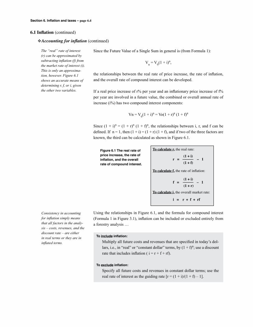
Section 6. Inflation and taxes – page 6.4
Since the Future Value of a Single Sum in general is (from Formula 1):
Vn = V0(1 + i)n,
the relationships between the real rate of price increase, the rate of inflation, and the overall rate of compound interest can be developed.
If a real price increase of r% per year and an inflationary price increase of f% per year are involved in a future value, the combined or overall annual rate of increase (i%) has two compound interest components:
Vn = V0(1 + i)n = Vo(1 + r)n (1 + f)n
Since (1 + i)n = (1 + r)n (1 + f)n, the relationships between i, r, and f can be defined. If n = 1, then (1 + i) = (1 + r) (1 + f), and if two of the three factors are known, the third can be calculated as shown in Figure 6.1.
Using the relationships in Figure 6.1, and the formula for compound interest (Formula 1 in Figure 3.1), inflation can be included or excluded entirely from a forestry analysis …
To include inflation: Multiply all future costs and revenues that are specified in today’s dol-
lars, i.e., in “real” or “constant dollar” terms, by (1 + f)n; use a discount rate that includes inflation ( i = r + f + rf).
To exclude inflation: Specify all future costs and revenues in constant dollar terms; use the
real rate of interest as the guiding rate [r = (1 + i)/(1 + f) – 1].
The “real” rate of interest (r) can be approximated by subtracting inflation (f) from the market rate of interest (i). This is only an approxima-tion, however. Figure 6.1 shows an accurate means of determining r, f, or i, given the other two variables.
Consistency in accounting for inflation simply means that all factors in the analy-sis – costs, revenues, and the discount rate – are either in real terms or they are in inflated terms.
Figure 6.1 The real rate ofprice increase, the rate of inflation, and the overall rate of compound interest.
To calculate r, the real rate:
To calculate f, the rate of inflation:
To calculate i, the overall market rate:
r = – 1(1 + i)
(1 + f)
f = – 1(1 + i)
(1 + r)
i = r + f + rf
6.1 Inflation (continued)
vAccounting for inflation (continued)
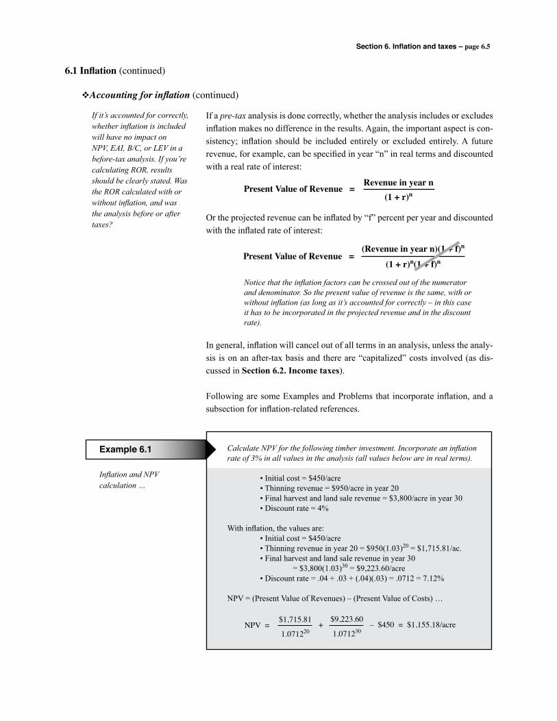
Section 6. Inflation and taxes – page 6.5
6.1 Inflation (continued)
vAccounting for inflation (continued)
If a pre-tax analysis is done correctly, whether the analysis includes or excludes inflation makes no difference in the results. Again, the important aspect is con-sistency; inflation should be included entirely or excluded entirely. A future revenue, for example, can be specified in year “n” in real terms and discounted with a real rate of interest:
Or the projected revenue can be inflated by “f” percent per year and discounted with the inflated rate of interest:
In general, inflation will cancel out of all terms in an analysis, unless the analy-sis is on an after-tax basis and there are “capitalized” costs involved (as dis-cussed in Section 6.2. Income taxes).
Following are some Examples and Problems that incorporate inflation, and a subsection for inflation-related references.
If it’s accounted for correctly, whether inflation is included will have no impact on NPV, EAI, B/C, or LEV in a before-tax analysis. If you’re calculating ROR, results should be clearly stated. Was the ROR calculated with or without inflation, and was the analysis before or after taxes?
Present Value of Revenue =Revenue in year n
(1 + r)n
Notice that the inflation factors can be crossed out of the numerator and denominator. So the present value of revenue is the same, with or without inflation (as long as it’s accounted for correctly – in this case it has to be incorporated in the projected revenue and in the discount rate).
Present Value of Revenue =(Revenue in year n)(1 + f)n
(1 + r)n(1 + f)n
Inflation and NPVcalculation …
Example 6.1 Calculate NPV for the following timber investment. Incorporate an inflation rate of 3% in all values in the analysis (all values below are in real terms).
• Initial cost = $450/acre • Thinning revenue = $950/acre in year 20 • Final harvest and land sale revenue = $3,800/acre in year 30 • Discount rate = 4%
With inflation, the values are: • Initial cost = $450/acre • Thinning revenue in year 20 = $950(1.03)20 = $1,715.81/ac. • Final harvest and land sale revenue in year 30 = $3,800(1.03)30 = $9,223.60/acre • Discount rate = .04 + .03 + (.04)(.03) = .0712 = 7.12%
NPV = (Present Value of Revenues) – (Present Value of Costs) …
NPV =$1,715.81
1.071220
$9,223.60
1.071230+ – $450 = $1,155.18/acre
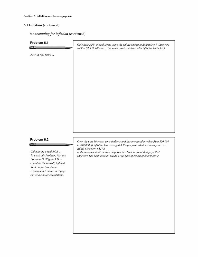
Section 6. Inflation and taxes – page 6.6
6.1 Inflation (continued)
vAccounting for inflation (continued)
NPV in real terms …
Problem 6.1 Calculate NPV in real terms using the values shown in Example 6.1. (Answer: NPV = $1,155.18/acre … the same result obtained with inflation included.)
Calculating a real ROR …To work this Problem, first use Formula 11 (Figure 3.1) to calculate the overall, inflated ROR on the investment. (Example 6.2 on the next page shows a similar calculation.)
Problem 6.2 Over the past 10 years, your timber stand has increased in value from $20,000 to $48,000. If inflation has averaged 4.1% per year, what has been your real ROR? (Answer: 4.85%)Is the investment attractive compared to a bank account that pays 5%? (Answer: The bank account yields a real rate of return of only 0.86%)
Section 6. Inflation and taxes – page 6.7
6.1 Inflation (continued)
vAccounting for inflation (continued)
Real price increases for timber in a specific area …
Problem 6.3 Using the methods demonstrated in Example 6.2, calculate the real rate of change in prices for standing timber between 1985 and 2010. Assume that prices for standing timber of similar species, size, and quality averaged $225/MBF in your area in 1985, and they averaged $475/MBF in 2010. Assume that inflation averaged 2% per year over the 25-year period. (Answer: r = 1.03% per year)
A non-forestry example …
Example 6.2 The cost of a U.S. postage stamp for mailing first class letters increased from 4 cents in 1960 to 44 cents in 2010. Was there a real price increase in U.S. postage costs if inflation over the period averaged 3.7% per year?
First, calculate the rate of compound interest that makes 4 cents equal to 44 cents over a 50-year period. To do this, we apply Formula 11 in Figure 3.1:
The inflated rate of price increase was 4.91%/year, and we can use the equa-tion shown in Figure 6.1 to calculate r, given i and f:
The price increase was 1.17%/year over and above the increase attributed to inflation. In this particular example, a close estimate of the real rate of increase (r) is obtained by simply subtracting the rate of inflation (f) from the rate of price increase (i). That is, r is approximately 4.91% – 3.7% = 1.21%.
i = – 1 = .0491 = 4.91% .44
.04
1/50
r = – 1 = .0117 = 1.17% 1.0491
1.037
Section 6. Inflation and taxes – page 6.8
6.1 Inflation (continued)
vAccounting for inflation (continued)
When using interest rates as a “yardstick” for comparing alternatives, the rates must be comparable in terms of taxes and inflation, and possibly also in terms of factors such as investment duration, risk, and liquidity.
Problem 6.4 You’ve estimated an annual rate of return of 7.9% for a specific timberland investment. In the process, you used today’s prices and costs, i.e., you didn’t inflate the values using a projected rate of inflation. Is this an acceptable invest-ment if your alternative rate of return is defined by what you can earn in an investment account that will pay 8% interest over the next 20 years?
A timber priceprojection …
Example 6.3 In a specific forestry investment analysis, you need a timber price projected for the year 2030 (for this Example, “today” is 2010). You assume that inflation will average 4% per year over the 20-year period, and you’ve read a recently-completed study that projects that real timber prices will increase at a compound annual rate of 1.5% for the “foreseeable” future. If you assume timber prices will increase at an average rate of 4% with inflation plus 1.5% in real terms, what is the price projected for 2030? Today’s price is $410/MBF.
The overall rate of price increase that’s projected is:
i = r + f + rf (from Figure 6.1)
So in this Example, the projected rate of price increase is:
i = .015 + .04 + (.015)(.04) = 5.56%
The price projected for the year 2030 is therefore:
$410 (1.0556)20 = $1,209.96/MBF
Note that price estimates can also be made by treating the real and inflation-ary rates of increase separately …
$410 (1.015)20(1.04)20 = $1,209.96/MBF.
Section 6. Inflation and taxes – page 6.9
6.1 Inflation (continued)
vReferences that relate to inflation
Bullard, S.H. and W.D. Klemperer. 1986. Effects of inflation on after-tax present values where business costs are capitalized. Mid-South Bus. J. 6(2):11–13.
Bullard, S.H., T.A. Monaghan and T.J. Straka. 1986. Introduction to forest valuation and investment analysis (VIII. Investment Analysis – Accounting for Inflation, p.81). Public. 1546, Miss. Coop. Ext. Serv., Miss. State Univ., Mississippi State, MS, 131p.
Clutter, J.L., J.C. Fortson, L.V. Pienaar, G.H. Brister and R.L. Bailey. 1983. Timber Management: A Quantita-tive Approach (Chapter 5, Section 5.4 Adjusting for Anticipated Inflation). John Wiley & Sons, New York, 333p.
Flick, W.A. 1976. A note on inflation and forest investments. For. Sci. 22(1):30–32.
Gunter, J.E. and H.L. Haney, Jr. 1984. Essentials of Forestry Investment Analysis (Inflation and Real Price Appreciation, p. 108). Copyright Gunter–Haney, 337 p.
Gregersen, H.M. 1975. Effect of inflation on evaluation of forestry investments. J. For. 73:570–572.
Hotvedt, J.E. 1982. Inflation and the capital budgeting process. South. J. Appl. For. 6(4):195–200.
Klemperer, W.D. 1979. Inflation and present value of timber income after taxes. J. For. 77:94–96.
Klemperer, W.D. 1987. Possible misinterpretations of equivalent annual incomes in inflationary times. North. J. Appl. For. 4:210–211.
Klemperer, W.D. 1996. Forest Resource Economics and Finance. McGraw-Hill, New York, 551p.
Leuschner, W.A. 1984. Introduction to Forest Resource Management (Part I, Chapter 7. Adjusting for Infla-tion). John Wiley & Sons, New York, 298p.
Uys, H.J.E. 1990. Determining optimal financial rotations under inflationary conditions. S. African For. J. 154:18–23.
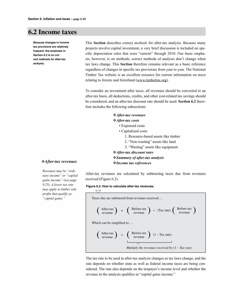
Section 6. Inflation and taxes – page 6.10
This Section describes correct methods for after-tax analysis. Because many projects involve capital investment, a very brief discussion is included on spe-cific depreciation rules that were “current” through 2010. Our basic empha-sis, however, is on methods; correct methods of analysis don’t change when tax laws change. This Section therefore remains relevant as a basic reference regardless of changes in specific tax provisions from year to year. The National Timber Tax website is an excellent resource for current information on taxes relating to forests and forestland (www.timbertax.org).
To consider an investment after taxes, all revenues should be converted to an after-tax basis, all deductions, credits, and other cost-related tax savings should be considered, and an after-tax discount rate should be used. Section 6.2 there-fore includes the following subsections:
vAfter-tax revenues vAfter-tax costs • Expensed costs • Capitalized costs 1. Resource-based assets like timber 2. “Non-wasting” assets like land 3. “Wasting” assets like equipment vAfter-tax discount rates vSummary of after-tax analysis vIncome tax references
After-tax revenues are calculated by subtracting taxes due from revenues received (Figure 6.2).
6.2 Income taxesBecause changes in income tax provisions are relatively frequent, the emphasis in Section 6.2 is on cor-rect methods for after-tax analysis.
vAfter-tax revenues
Revenues may be “ordi-nary income” or “capital gains income” (see page 9.25). A lower tax rate may apply to timber sale profits that qualify as “capital gains.”
Figure 6.2. How to calculate after-tax revenues.
Taxes due are subtracted from revenues received …
Which can be simplified to …
( After-taxrevenue ( ( Before-tax
revenue (= – (Tax rate) ( Before-taxrevenue (
( After-taxrevenue ( ( Before-tax
revenue (= (1 – Tax rate)
Multiply the revenues received by (1 – Tax rate)
The tax rate to be used in after-tax analysis changes as tax laws change, and the rate depends on whether state as well as federal income taxes are being con-sidered. The rate also depends on the taxpayer’s income level and whether the revenue in the analysis qualifies as “capital gains income.”
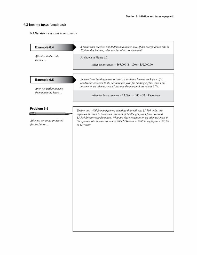
Section 6. Inflation and taxes – page 6.11
6.2 Income taxes (continued)
vAfter-tax revenues (continued)
After-tax revenues projected for the future …
Problem 6.5 Timber and wildlife management practices that will cost $1,700 today are expected to result in increased revenues of $400 eight years from now and $3,300 fifteen years from now. What are these revenues on an after-tax basis if the appropriate income tax rate is 28%? (Answer = $288 in eight years; $2,376 in 15 years)
After-tax timber sale income …
Example 6.4 A landowner receives $65,000 from a timber sale. If her marginal tax rate is 20% on this income, what are her after-tax revenues?
As shown in Figure 6.2,
After-tax revenues = $65,000 (1 – .20) = $52,000.00
After-tax timber income from a hunting lease …
Example 6.5 Income from hunting leases is taxed as ordinary income each year. If a landowner receives $5.00 per acre per year for hunting rights, what’s the income on an after-tax basis? Assume the marginal tax rate is 31%.
After-tax lease revenue = $5.00 (1 – .31) = $3.45/acre/year
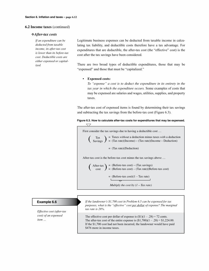
Section 6. Inflation and taxes – page 6.12
6.2 Income taxes (continued)
vAfter-tax costs Legitimate business expenses can be deducted from taxable income in calcu-lating tax liability, and deductible costs therefore have a tax advantage. For expenditures that are deductible, the after-tax cost (the “effective” cost) is the cost after the tax savings have been considered.
There are two broad types of deductible expenditures, those that may be “expensed” and those that must be “capitalized.”
• Expensed costs: To “expense” a cost is to deduct the expenditure in its entirety in the
tax year in which the expenditure occurs. Some examples of costs that may be expensed are salaries and wages, utilities, supplies, and property taxes.
The after-tax cost of expensed items is found by determining their tax savings and subtracting the tax savings from the before-tax cost (Figure 6.3).
If an expenditure can be deducted from taxable income, its after-tax cost is lower than its before-tax cost. Deductible costs are either expensed or capital-ized.
Figure 6.3. How to calculate after-tax costs for expenditures that may be expensed.
First consider the tax savings due to having a deductible cost …
After-tax cost is the before-tax cost minus the tax savings above …
( TaxSavings (= Taxes without a deduction minus taxes with a deduction
= (Tax rate)(Income) – (Tax rate)(Income – Deduction)
= (Tax rate)(Deduction)
( After-taxcost (
Multiply the cost by (1 – Tax rate)
= (Before-tax cost) – (Tax savings)= (Before-tax cost) – (Tax rate)(Before-tax cost)
= (Before-tax cost)(1 – Tax rate)
Effective cost (after-tax cost) of an expenseditem …
If the landowner’s $1,700 cost in Problem 6.5 can be expensed for tax purposes, what is the “effective” cost per dollar of expense? The marginal tax rate is 28%.
The effective cost per dollar of expense is ($1)(1 – .28) = 72 cents.The after-tax cost of the entire expense is ($1,700)(1 – .28) = $1,224.00.If the $1,700 cost had not been incurred, the landowner would have paid $476 more in income taxes.
Example 6.6

Section 6. Inflation and taxes – page 6.13
6.2 Income taxes (continued)
vAfter-tax costs (continued)
After-tax NPV
Problem 6.6 What’s the landowner’s after-tax NPV in Problem 6.5 assuming the $1,700 cost can be expensed? Use an after-tax discount rate of 4.68%. (Answer = $172.10)
After-tax costs of items that can be expensed for income tax purposes …
Problem 6.7 List forestry-related items whose cost can be expensed, then list the before- and after-tax cost of each item (assume an appropriate tax rate).
Example:Tree planting dibble … Before-tax cost = $23.00 After-tax cost = $23.00 (1 – .31) = $15.87 (assuming a marginal rax rate of 31%)
Section 6. Inflation and taxes – page 6.14
6.2 Income taxes (continued)
vAfter-tax costs (continued) The second category of costs are those that must be “capitalized” for income tax purposes.
• Capitalized costs: Costs that are not deducted entirely in the year they occur are “capital-
ized.” For record-keeping purposes, these costs are assigned to a capi-tal account or “basis,” and they are deducted over time in one of three ways:
1. Certain resource-based assets like oil, gas, and timber – costs are deducted as the asset is used or “depleted.” The basis is called the “basis for depletion.”
2. “Non-wasting” assets like land – costs are deducted when the asset is sold.
3. “Wasting” assets like buildings and equipment – costs are deducted as the asset depreciates; the schedule for depreciation deductions is defined based on the type of asset and the expected length of service.
Timberland includes both timber and land (numbers 1 and 2 above), and when timberland is purchased or inherited, initial costs (market value in the case of inherited property) as well as subsequent costs must be allocated between a land account and a timber account:
Land account … The money you have invested in land can be deducted from the revenue obtained when the land is sold.
Timber account … The money you have invested in timber can be deducted when the timber is sold (depleted). For partial sales, calculate a depletion allowance as shown below. After each timber sale (after each depletion allowance is deducted) adjust the basis for depletion.
• The depletion rate is the amount of money you can deduct per unit of timber volume harvested:
Depletion rate = (Basis for depletion ÷ Total volume)
• The depletion allowance is the amount of money you can deduct in total after a specific timber sale. It’s obtained by multiplying the deple-tion rate by the total volume of timber harvested:
Depletion allowance = (Depletion rate) x (Volume cut)
For income tax purposes, legitimate business-related costs are either expensed or capitalized.
NOTE: A simple interpreta-tion of the depletion allow-
ance for a given timber sale is to deduct a percentage of
the basis equal to the per-centage of the timber that’s
harvested. If 100% of the timber is cut, for example,
deduct 100% of the basis. If a thinning removes 30% of
the volume, deduct 30%, etc.
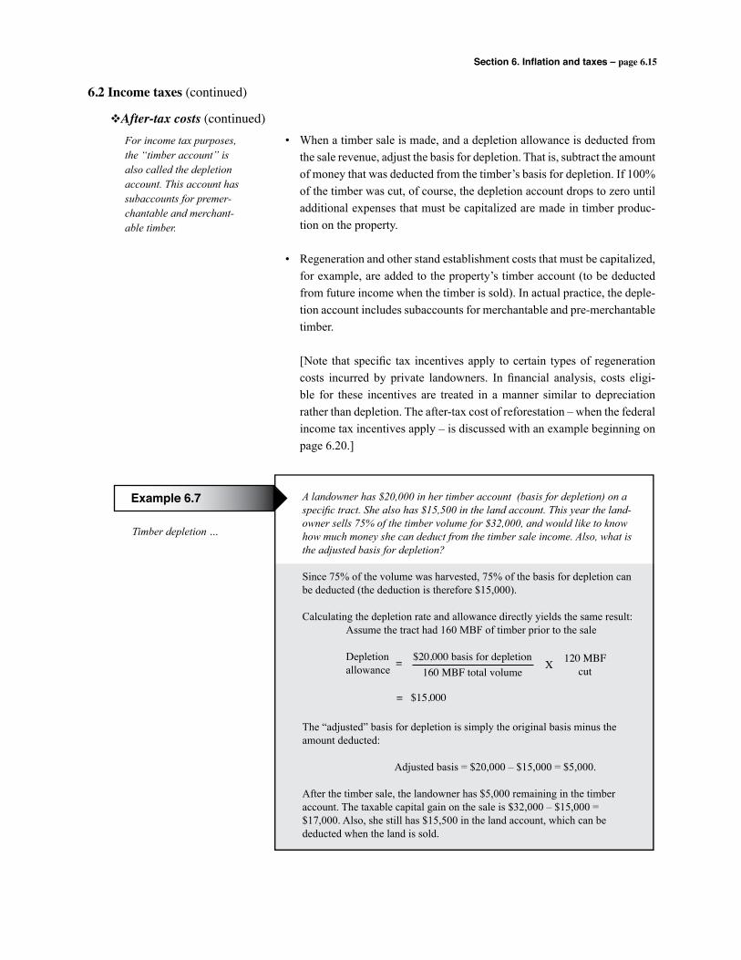
Section 6. Inflation and taxes – page 6.15
6.2 Income taxes (continued)
vAfter-tax costs (continued) • When a timber sale is made, and a depletion allowance is deducted from
the sale revenue, adjust the basis for depletion. That is, subtract the amount of money that was deducted from the timber’s basis for depletion. If 100% of the timber was cut, of course, the depletion account drops to zero until additional expenses that must be capitalized are made in timber produc-tion on the property.
• Regeneration and other stand establishment costs that must be capitalized, for example, are added to the property’s timber account (to be deducted from future income when the timber is sold). In actual practice, the deple-tion account includes subaccounts for merchantable and pre-merchantable timber.
[Note that specific tax incentives apply to certain types of regeneration costs incurred by private landowners. In financial analysis, costs eligi-ble for these incentives are treated in a manner similar to depreciation rather than depletion. The after-tax cost of reforestation – when the federal income tax incentives apply – is discussed with an example beginning on page 6.20.]
For income tax purposes, the “timber account” is also called the depletion account. This account has subaccounts for premer-chantable and merchant-able timber.
Timber depletion …
A landowner has $20,000 in her timber account (basis for depletion) on a specific tract. She also has $15,500 in the land account. This year the land-owner sells 75% of the timber volume for $32,000, and would like to know how much money she can deduct from the timber sale income. Also, what is the adjusted basis for depletion?
Since 75% of the volume was harvested, 75% of the basis for depletion can be deducted (the deduction is therefore $15,000).
Calculating the depletion rate and allowance directly yields the same result: Assume the tract had 160 MBF of timber prior to the sale
Depletion allowance
The “adjusted” basis for depletion is simply the original basis minus the amount deducted:
Adjusted basis = $20,000 – $15,000 = $5,000.
After the timber sale, the landowner has $5,000 remaining in the timber account. The taxable capital gain on the sale is $32,000 – $15,000 = $17,000. Also, she still has $15,500 in the land account, which can be deducted when the land is sold.
Example 6.7
= $20,000 basis for depletion160 MBF total volume
X 120 MBFcut
= $15,000
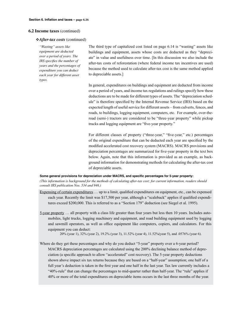
Section 6. Inflation and taxes – page 6.16
6.2 Income taxes (continued)
vAfter-tax costs (continued) The third type of capitalized cost listed on page 6.14 is “wasting” assets like buildings and equipment, assets whose costs are deducted as they “depreci-ate” in value and usefulness over time. [In this discussion we also include the after-tax costs of reforestation (where federal income tax incentives are used) because the method used to calculate after-tax cost is the same method applied to depreciable assets.]
In general, expenditures on buildings and equipment are deducted from income over a period of years, and income tax regulations and rulings specify how these deductions are to be made for different types of assets. The “depreciation sched-ule” is therefore specified by the Internal Revenue Service (IRS) based on the expected length of useful service for different assets – from culverts, fences, and roads, to buildings, logging equipment, computers, etc. For example, over-the-road (semi-) tractors are considered to be “three-year property” while pickup trucks and logging equipment are “five-year property.”
For different classes of property (“three-year,” “five-year,” etc.) percentages of the original expenditure that can be deducted each year are specified by the modified accelerated cost recovery system (MACRS). MACRS provisions and depreciation percentages are summarized for five-year property in the text box below. Again, note that this information is provided as an example, as back-ground information for demonstrating methods for calculating the after-tax cost of depreciable assets.
“Wasting” assets like equipment are deducted over a period of years. The IRS specifies the number of years and the percentages of expenditure you can deduct each year for different asset types.
Some general provisions for depreciation under MACRS, and specific percentages for 5-year property:(This information is background for the methods of calculating after-tax cost; for current information, readers should consult IRS publication Nos. 534 and 946.)
Expensing of certain expenditures … up to a limit, qualified expenditures on equipment, etc., can be expensed each year. Recently the limit was $17,500 per year, although a “scaleback” applies if qualified expendi-tures exceed $200,000. This is referred to as a “Section 179” deduction (see Siegel et al. 1995).
5-year property … all property with a class life greater than four years but less then 10 years. Includes auto-mobiles, light trucks, logging machinery and equipment, and road building equipment used by logging and sawmill operators, as well as office equipment like computers, copiers, and calculators. For this equipment you can deduct:
20% (year 1), 32% (year 2), 19.2% (year 3), 11.52% (year 4), 11.52%(year 5), and .0576% (year 6).
Where do they get these percentages and why do you deduct “5-year” property over a 6-year period? MACRS depreciation percentages are calculated using the 200% declining balance method of depre-
ciation (a specific approach to allow “accelerated” cost recovery). The 5-year property deductions shown above impact six tax returns because they are based on a “half-year” assumption; one half of a full year’s deduction is taken in the first year and one half in the last year. Tax law currently includes a “40%-rule” that can change the percentages to mid-quarter rather than half-year. The “rule” applies if 40% or more of the total expenditures on depreciable items occurs in the last three months of the year.

Section 6. Inflation and taxes – page 6.17
6.2 Income taxes (continued)
vAfter-tax costs (continued) Earlier, when we calculated the after-tax cost of items that can be expensed, we calculated the tax savings due to having a deduction from taxable income, and we subtracted the savings from the item’s cost (Figure 6.3 on page 6.12). With capitalized costs of depreciating assets like equipment, however, deductions are spread over several years, and to calculate their tax savings we need to account for the time value of money. The basic method involves: discounting the tax savings that will occur from each deduction (they occur in the future so we calculate their total present value), and subtracting the total present value of tax savings from the cost of the item (Figure 6.4).
To estimate the after-tax cost of a depreciating asset …discount the tax savings from each depreciation deduction to the present and subtract them from the origi-nal expenditure.
Figure 6.4. How to calculate after-tax costs for equipment and other expenditures that are depreciated over time.
Each deduction results in a tax savings of (Tax Rate) x (Deduction), and we discount each of the “n” tax savings to year 0. This total is subtracted from the item’s before-tax cost:
Where “d” is the total number of deductions, “n” is the year each deduction occcurs, and “i” is an after-tax discount rate.
( After-taxcost ( ( Before-tax
cost (=(Tax rate)(Deduction)
(1 + i)n∑n = 0
d
–
After-tax cost of askidder …
What’s the after-tax cost of a skidder with a purchase price of $175,000? Assume the buyer is in a 34% marginal tax bracket. and uses an after-tax discount rate of 6% (after-tax discount rates are discussed in the next subsection).
For this example, we apply the schedule of deductions shown for 5-year property (listed in the text box on page 6.16). There are six deductions:
The “effective” cost of the skidder is:
$175,000 – $50,731.14 = $124,268.86
Example 6.8
Each tax savings is discounted to year 0 as shown in Figure 6.4 (in this Example using a 6% after-tax discount rate).
1 ($175,000) (.2000) (.34) $11,226.422 ($175,000) (.3200) (.34) $16,945.533 ($175,000) (.1920) (.34) $9,591.814 ($175,000) (.1152) (.34) $5,429.335 ($175,000) (.1152) (.34) $5,122.016 ($175,000) (.0576) (.34) $2,416.04
YearDeduction in year n
Tax savings from the deduction in year n Present
Value ofTax Savings
Total Present Value of Tax Savings = $50,731.14
Section 6. Inflation and taxes – page 6.18
6.2 Income taxes (continued)
vAfter-tax costs (continued) In Example 6.8, notice that the deductions were assumed to occur in years 1 through 6. This means the first deduction isn’t received until a year from the equipment purchase. In any case, an assumption is necessary for discounting purposes. If we used 0 – 5 as the six years in the depreciation schedule, we would be assuming the first deduction occurs now (in year 0).
Another important point about calculating the after-tax cost of depreciable items can be seen in Example 6.8. In the column of deductions, notice that the initial cost of the skidder ($175,000) is repeated in each line. We can replace the $175,000 with $1 in example 6.8 and we will calculate a tax savings per dollar of initial cost.
In Example 6.8, if we replace $175,000 with $1, we calculate a tax savings of .28989 per dollar of before-tax cost (you’re asked to do this in Problem 6.8). Subtracting this amount from $1 yields the after-tax cost per dollar of before-tax cost. In this case, $1 - .28989 = .71011, or 71 cents per dollar. Our after-tax present value of costs for the skidder would be: ($175,000) (.71011) = $124,269.25 (not exactly the answer in Example 6.8 due to rounding error).
After-tax costs for any equipment in the 5-year property class, for anyone who’s in the 34% marginal tax bracket and has a 6% after-tax discount rate can be estimated by multiplying the purchase price by .71011. This value is therefore a multiplier that can be used to estimate other after-tax values. Multipliers for 5-year property (or other classes) can be developed exactly as demonstrated in Example 6.8 and Problem 6.8.
After-tax cost multipliers can also be determined for 7-year property, or any of the other useful life categories in tax regulations. Listed below, for example, are some example multipliers for 5-year and 7-year property, for tax rates of 28% and 34%.
To estimate the after-tax cost of an asset that must be depreciated, first obtain the depreciation schedule, the tax rate, and the discount rate. The after-tax cost can be estimated in total (as in Example 6.8), or per dollar of initial expense (as in Problem 6.8).
Multipliers for estimating the after-tax present value of costs for 5-year property and 7-year property, using marginal tax rates of 28% and 34% …
8% .75981 .70476 .76989 .71623 9% .76413 .71020 .77510 .72219 10% .76832 .71445 .78012 .72794 11% .77238 .72276 .78496 .72250 12% .77633 .72361 .78963 .73888
Before-taxDiscount Rate 28% 34% 28% 34%
5-year Property 7-year Property
Once developed, multipli-ers can be used to quickly estimate the after-tax pres-ent value of capitalized costs that are recovered through depreciation.
An assumption used in calculating the multipliers shown here is that the after tax discount rate is (Before tax Rate)(1–TaxRate) … see page 6.22.
Section 6. Inflation and taxes – page 6.19
6.1 Income taxes (continued)
vAfter-tax costs (continued)
After-tax cost of a pickuptruck …
Problem 6.8 If you purchase a pickup truck for use in your business for $26,500, what’s the “effective” cost on an after-tax basis? Assume a 34% tax rate and a before-tax cost of capital of 8%. [This means the after-tax cost of capital is (1–.34)(.08) = 5.28% using the “rule-of-thumb” adjustment described on page 6.22.] For this problem, use the depreciation schedule for five-year property shown in the text box on page 6.16. (Answer = $18,676.11)
After-tax cost using a pre-calculated multiplier …
Example 6.8 In Problem 6.8, the “effective” cost of a pickup truck was calculated. The cost can also be calculated using a pre-calculated multiplier for 5-year property.
The cost of the pickup truck in after-tax present value terms can be calcu-lated using the multiplier on page 6.18 for 5-year property, a 34% tax rate, and an 8% before-tax discount rate:
Effective cost = ($26,500) (.70476) = $18,676.14
Section 6. Inflation and taxes – page 6.20
6.2 Income taxes (continued)
vAfter-tax costs (continued)
Earlier in this subsection we stated that federal income tax incentives were available for qualified reforestation expenditures. The after-tax cost of refores-tation, considering the tax incentives, are determined in exactly the same way that we determined the after-tax cost of equipment and other assets whose costs are recovered through depreciation. In this subsection we therefore include the following example calculation of the after-tax cost of reforestation.
Although the exact provisions of the tax law that relate to reforestation may change, our purpose is to demonstrate the general method used to calculate after-tax reforestation costs. For this demonstration, we assume:
• Total reforestation costs are less than or equal to $10,000.
• The landowner claims a 10% tax credit and amortizes 95% of the refores-tation expenses. The amortization is 1/14th of 95% of the expenses in the first tax year, 1/7th of 95% in each of the next six tax years, and 1/14th in the last tax year.
• Reforestation expenses are incurred toward the end of the tax year. (If we had assumed the expenses were toward the beginning of the tax year we’d discount the tax savings from years 1–8 rather than years 0–7.)
• Any cost-shares received are not included as taxable income.
As a specific example, assume a landowner with a discount rate of 10%, a 28% marginal tax rate, and an opportunity to receive 50% cost-shares. If this land-owner spends $10,000 on reforestation in November/December we can esti-mate the “effective” or after-tax cost as itemized in the example on page 6.21.
Notice that the landowner immediately (year 0) receives $5,000 in cost sharing, a $500 tax credit, and an additional reduction in taxes of $95. He also receives tax savings from deductions in each of the next seven years.
After-tax costs of refor-estation – the method is the same method used to determine after-tax costs for equipment.
The basic method is to determine the present value of all tax savings, cost shares, etc., and subtract the total of all savings from the initial cost.
In calculating after-tax reforestation costs, for the results to be most accurate the discount rate should include inflation.
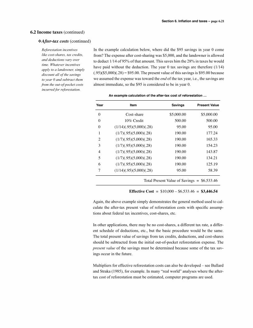
Section 6. Inflation and taxes – page 6.21
6.2 Income taxes (continued)
vAfter-tax costs (continued)
In the example calculation below, where did the $95 savings in year 0 come from? The expense after cost-sharing was $5,000, and the landowner is allowed to deduct 1/14 of 95% of that amount. This saves him the 28% in taxes he would have paid without the deduction. The year 0 tax savings are therefore (1/14)(.95)($5,000)(.28) = $95.00. The present value of this savings is $95.00 because we assumed the expense was toward the end of the tax year, i.e., the savings are almost immediate, so the $95 is considered to be in year 0.
Reforestation incentives like cost-shares, tax credits, and deductions vary over time. Whatever incentives apply to a landowner, simply discount all of the savings to year 0 and subtract them from the out-of-pocket costs incurred for reforestation.
An example calculation of the after-tax cost of reforestation …
Year Item Savings Present Value
0 Cost-share $5,000.00 $5,000.000 10% Credit 500.00 500.000 (1/14)(.95)(5,000)(.28) 95.00 95.001 (1/7)(.95)(5,000)(.28) 190.00 177.242 (1/7)(.95)(5,000)(.28) 190.00 165.333 (1/7)(.95)(5,000)(.28) 190.00 154.234 (1/7)(.95)(5,000)(.28) 190.00 143.875 (1/7)(.95)(5,000)(.28) 190.00 134.216 (1/7)(.95)(5,000)(.28) 190.00 125.197 (1/14)(.95)(5,000)(.28) 95.00 58.39
Total Present Value of Savings = $6,533.46
Effective Cost = $10,000 – $6,533.46 = $3,446.54
Again, the above example simply demonstrates the general method used to cal-culate the after-tax present value of reforestation costs with specific assump-tions about federal tax incentives, cost-shares, etc.
In other applications, there may be no cost-shares, a different tax rate, a differ-ent schedule of deductions, etc., but the basic procedure would be the same. The total present value of savings from tax credits, deductions, and cost-shares should be subtracted from the initial out-of-pocket reforestation expense. The present value of the savings must be determined because some of the tax sav-ings occur in the future.
Multipliers for effective reforestation costs can also be developed – see Bullard and Straka (1985), for example. In many “real world” analyses where the after-tax cost of reforestation must be estimated, computer programs are used.
Section 6. Inflation and taxes – page 6.22
6.2 Income taxes (continued)
vAfter-tax discount rate
Interest paid on business-related loans is deductible from income for tax pur-poses. The interest is deducted in the year it’s paid, i.e., it is expensed, and the after-tax “cost” of interest is therefore determined exactly like the after-tax cost of any other expensed item:
After-tax Discount Rate = (Before-tax Rate) (1 – Tax Rate)
The after-tax discount rate can be estimated simply by multiplying the before tax rate by (1 – tax rate).
After-tax discount rate …
Example 6.9 What is a landowner’s estimated after-tax discount rate if the before-tax rate is 12%? The marginal tax rate is 28%.
After-tax Rate = (.12) ( 1 – .28) = 8.64%
After-tax tate of return …
Example 6.10 Assume that you’ve calculated an after-tax rate of return of 6.3% for a specific forestry investment. You included inflation in the analysis. Your esti-mated ROR is therefore after-taxes, with inflation. Is this rate comparable to 8% interest that can be earned at a bank ?
Considering only taxes and inflation (ignoring risk, liquidity and other potential considerations), the rates aren’t comparable until both are either after-tax or before-tax, and both are either with or without inflation.
After-tax bank rate = (.08) (1 – .28) = 5.76%
In this case, the forestry ROR was estimated as 6.3% after taxes, with infla-tion. The bank rate is with inflation, but is not on an after-tax basis. We can, however, make the bank rate comparable by converting it to an equivalent after-tax rate.
The above method of adjusting discount rates for income taxes was termed the “rule-of-thumb” method by Campbell and Colletti (1990). These authors investigated the rule-of-thumb’s accuracy, and concluded that it is “generally satisfactory” for “the private landowner whose investment alternatives (other than the forestry practice under evaluation) are limited to opportunities such as land rental, taxable bonds, or bank certificates of deposit.”
The rule-of-thumb discount rate adjustment for taxes should only be applied to discount rates that are specified in nominal (inflated) terms. Formulas to adjust real interest rates for taxes are presented in Bullard, Straka, and Caulfield (2001). A simple three-step process to adjust discount rates for income taxes and inflation, including adjusting real rates for taxes, is presented in Bullard and Gunter (2000).
Section 6. Inflation and taxes – page 6.23
6.2 Income taxes (continued)
vSummary of after-tax analysis
To account for taxes in forestry or other investment analysis, convert all costs and revenues to an after-tax basis, and calculate all present values using an after-tax discount rate. If the investment has costs that must be capitalized for tax purposes, the discount rate and all costs and revenues should include infla-tion.
Specific steps for after-tax analysis …
1. Convert taxable revenues to after-tax revenues:
After-tax revenue = (Before-tax revenue)(1 – Tax rate)
• If the taxable revenue is from a timber sale and a depletion allow-ance applies, the depletion allowance should be subtracted from the timber sale income before multiplying by (1 – Tax rate).
• If the taxable revenue is from the sale of land, or land and timber together, deduct the capitalized costs in the land account and the timber account from the revenues before multiplying by (1 – Tax rate).
2. For all costs other than the capitalized costs of land and/or timber, con-vert costs to after-tax costs:
• If the costs can be expensed …
After-tax cost = (Before-tax cost)(1 – Tax rate)
• If the costs must be capitalized (like buildings, equipment, or refor-estation) …
calculate the after-tax present value of costs by discounting all future tax savings to the present and subtracting their total from the original expense incurred.
3. Use an after-tax discount rate to calculate NPV, B/C or other financial criteria (using the after-tax revenues and costs from steps 1 and 2):
After-tax discount rate = (Before-tax rate) (1 – tax rate) This adjustment is a “rule-of-thumb” that should only be applied to
nominal (inflated) interest rates.
The Examples and Problems in Section 6.2 demonstrated “steps” to follow in after-tax analysis. For more information on income taxes and forestry investments, see the references listed in the following subsection.
Section 6. Inflation and taxes – page 6.24
6.2 Income taxes (continued)
vIncome tax references
Bettinger, P., H.L. Haney, and W.C. Siegel. 1989. The impact of federal and state income taxes on timber income in the South following the 1986 Tax Reform Act. South. J. Appl. For. 13:196–203.
Bullard, S.H., T.A. Monaghan and T.J. Straka. 1986. Introduction to forest valuation and investment analysis (VII. Investment Analysis – Accounting for Taxes, p.62). Public. 1546, Miss. Coop. Ext. Serv., Miss. State Univ., Mississippi State, MS, 131p.
Bullard, S.H. 1985. Reforestation timing influences after-tax present value of costs. J. For. 83(9):561.
Bullard, S.H. and J.E. Gunter. 2000. Adjusting discount rates for income taxes and inflation: A three-step process. South. J. Appl. For. 24(4):193-195.
Bullard, S.H. and T.J. Straka. 1985. What is your “effective” rate of reforestation cost? For. Farm. 45(1):16–17.
Bullard, S.H. and T.J. Straka. 1992. A note on after-tax analysis where capitalized costs are depreciated. North. J. Appl. For. 9(1):31,32.
Bullard, S.H., T.J. Straka and J.P. Caulfield. 2001. Inflation and the rule-of-thumb method of adjusting the discount rate for income taxes. Can. J. For. Res. 31(1):52-58.
Campbell, G.E. and J.P. Colletti. 1990. An investigation of the rule-of-thumb method of estimating after tax rates of return. For. Sci. 36(4):878–893.
Clutter, J.L., J.C. Fortson, L.V. Pienaar, G.H. Brister and R.L. Bailey. 1983. Timber Management: A Quantita-tive Approach (Chapter 6, Section 6.1. Federal Income Taxes). John Wiley & Sons, New York, 333p.
Dicke, S.G. and D.A. Gaddis. 2006. Basics of basis. Publ. 1983, Miss. State Univ. Ext. Serv., Miss. State Univ., Mississippi State, MS, 7p.
Dicke, S.G. and T.A. Monaghan. 2001. Handling reforestation expenses. Publ. 2102, Miss. State Univ. Ext. Serv., Miss. State Univ., Mississippi State, MS, 4p.
Gaddia, D.A., Dicke, S.G. and J.E. Gunter. 2006. Timber tax overview. Publ. 2307, Miss. State Univ. Ext. Serv., Miss. State Univ., Mississippi State, MS, 8p.
Gunter, J.E. and H.L. Haney, Jr. 1984. Essentials of Forestry Investment Analysis (Income Tax Consider-ations, p. 90). Copyright Gunter–Haney, 337 p.
Haney, H.L., Jr., W.L. Hoover, W.C. Siegel and J.L. Greene. 2001. Forest landowners’ guide to the federal income tax. Agric. Handb. 718, U.S. Dept. of Agric., Washington, D.C. 159p.
Haney, H.L., Jr., W.C. Siegel and L.M. Bishop. 2005. Federal income tax on timber: A key to your most fre-quently asked questions. R8-TP 34, USDA For. Serv., South. Region, Atlanta, GA, 23p.
Section 6. Inflation and taxes – page 6.25
6.2 Income taxes (continued)
vIncome tax references (continued)
Haney, H.L., Jr. 1991. Cover your “basis” on federal income tax. For. Farm., 28th Manual Edition, 50(3):49– 51.
Harris, P.E., Z.W. Daughtrey and C.A. Bock. 1998. Agricultural Tax Issues and Form Preparation. Tax Insight, Madison, WI, 427p.
Klemperer, W.D. 1996. Forest Resource Economics and Finance (Chapter 9, Forest Taxation, p. 267). McGraw-Hill, New York, 551p.
Leuschner, W.A. 1984. Introduction to Forest Resource Management (Part I, Chapter 8. Adjusting for Taxes). John Wiley & Sons, New York, 298p.
Section 6. Inflation and taxes – page 6.26
6.1 Inflation The most important aspect of accounting for inflation in forest valuation and
investment analysis is consistency. Inflation should either be included or excluded (consistently) in the discount rate and in all costs and revenues. If you’re consistent, whether you include or exclude inflation won’t impact your analysis results, unless the analysis is on an after-tax basis and capitalized costs are involved. If capitalized costs are involved, the analysis is most accu-rate if inflation is included and if the analysis is on an after-tax basis.
There are many examples of inconsistent treatment of inflation in forest valua-tion and investment analysis. A common mistake is to use an inflated discount rate (such as the rate paid by a bank) in an analysis where timber-related costs and revenues are uninflated.
If inflation is included in an analysis, the costs, revenues and discount rate are referred to as “nominal” or in “current dollars;” if inflation is excluded they’re said to be “real” or in “constant dollar” terms.
To include inflation in an analysis … Multiply all future costs and revenues that are specified in today’s dollars,
i.e., in real or “constant dollar” terms, by (1 + f)n and use a discount rate that includes inflation (in the factor above, “f” represents the rate of infla-tion in decimal percent).
To exclude inflation in an analysis … Specify all future costs and revenues in “constant dollar” terms and use the
real rate of interest as the discount rate: r = (1 + i)/(1 + f) – 1
6.2 Income taxes Section 6.2 emphasizes correct methods of after-tax analysis rather than spe-
cifics of current income tax regulations and rulings. To consider an investment after taxes, all revenues and costs should be converted to an after-tax basis, and an after-tax discount rate should be used.
vAfter-tax revenues A very simple formula can be used to convert before-tax revenues to an after-
tax basis:
6.3 Review of Section 6
Section 6. Inflation and taxes
( After-taxrevenue ( ( Before-tax
revenue (= ( 1 – Tax rate)
Section 6. Inflation and taxes – page 6.27
6.3 Review of Section 6 (continued)
6.2 Income taxes (continued)
vAfter-tax revenues (continued) In calculating after-tax revenues, the appropriate income tax rate to use is the
“marginal” rate, i.e., the tax rate paid on “additional” or “marginal” income.
vAfter-tax costs Legitimate business expenses are deductible from taxable income, and a
tax savings is therefore associated with such expenses. The after-tax cost of deductible expenditures is therefore less than their cost on a before-tax basis. There are two broad types of deductible expenditures, those that may be “expensed” and those that must be “capitalized:”
• Expensed costs – Costs like salaries, wages, utilities, and property taxes can be deducted entirely in the tax year in which they occur. Their after-tax cost is …
• Capitalized costs – Some costs must be assigned to a capital account or “basis;” they are not deducted entirely in the tax year in which they occur. They’re deducted over time in three ways …
1. Certain resource-based assets like oil, gas, and timber - costs are deducted as the asset is used or “depleted.” The basis is called the “basis for depletion” or the “depletion account.” In the case of timber it may also be referred as the “timber account.”
2. “Non-wasting” assets like land - costs are deducted when the asset is sold.
3. “Wasting” assets like buildings and equipment - costs are deducted as the asset depreciates (based on a defined schedule of depreciation).
When timberland is inherited or purchased, the asset has both timber and land (numbers one and two above). The timberland’s total value when acquired must be allocated to a land account and to a timber account, and the timber account may have subaccounts for premerchantable and mer-chantable timber.
( After-taxcost (= (Before-tax cost)(1 – Tax rate)

Section 6. Inflation and taxes – page 6.28
6.2 Income taxes (continued)
vAfter-tax costs (continued) When timber is sold, a depletion allowance is calculated, based on the basis for
depletion and the amount of timber sold. The depletion allowance is deducted from the timber sale revenue in determining income tax liability for the sale. After this deduction, the basis for depletion is “adjusted;” the new or adjusted basis for depletion is the former basis minus the depletion allowance that was claimed.
The third type of capitalized cost was “wasting” assets like buildings and equipment. For these asset types, costs are deducted as they depreciate in value and usefulness over time. Income tax regulations and rulings specify the depreciation schedule, or how these deductions are to be made for different types of assets.
With capitalized assets like equipment, the after-tax cost is calculated by dis-counting the tax savings (from each year’s depreciation deduction) to the pres-ent using an after-tax discount rate – their total is subtracted from the item’s before-tax cost:
There are federal income tax incentives for reforestation. For landowners that qualify, the after-tax cost of reforestation can be calculated using the same procedure for after-tax equipment costs. These incentives, availability of cost-share payments, and other factors involved with reforestation vary over time and in different areas. To calculate the “effective” cost of reforestation for a landowner, simply discount all of the savings to year zero and subtract them from the out-of-pocket costs.
vAfter-tax discount rate The third step in after-tax analysis is to use an after-tax discount rate:
After-tax Discount Rate = (Before-tax Rate) (1 – Tax Rate)
This “rule-of-thumb” adjustment should only be made to nominal interest rates. Section 6 concludes with a one-page vSummary of after-tax analysis, and a subsection titled vIncome tax references. Again, the objective of Sec-tion 6 was to introduce and demonstrate basic methods of after-tax analysis, rather than to present the specifics of current income tax provisions that relate to forest-related assets.
6.3 Review of Section 6 (continued)
( After-taxcost ( ( Before-tax
cost (=(Tax rate)(Deduction)n
(1 + i)n∑–
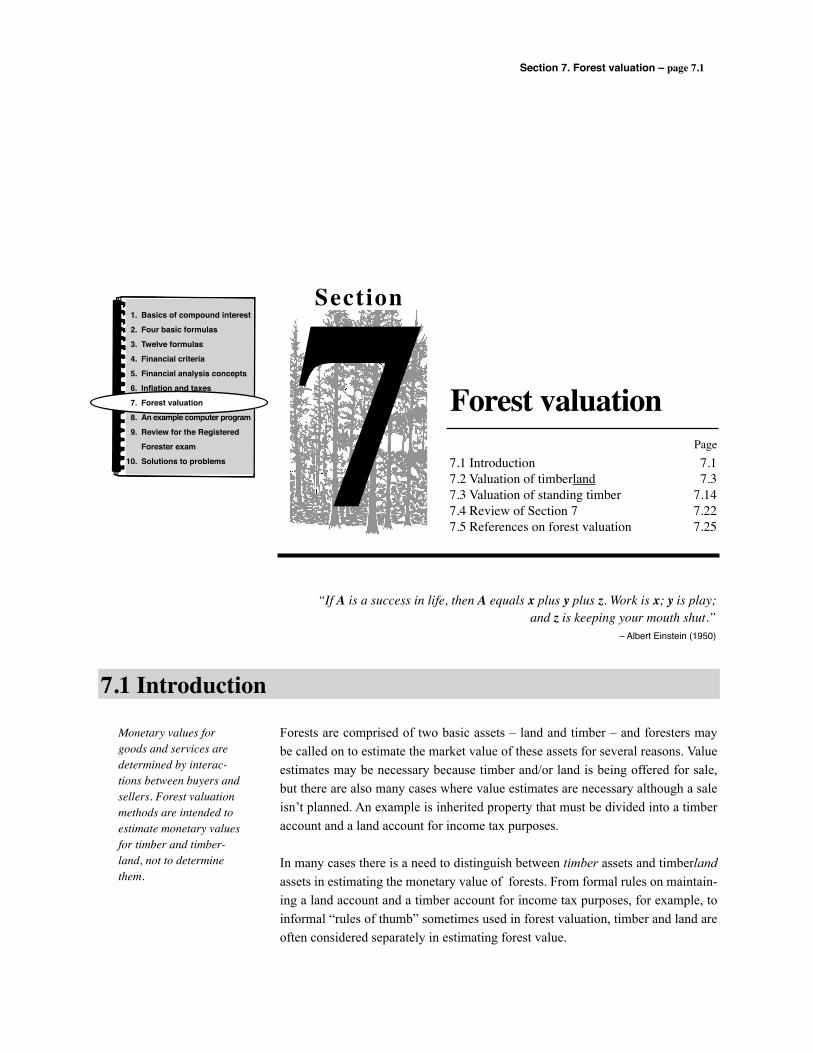
Section 7. Forest valuation – page 7.1
Forests are comprised of two basic assets – land and timber – and foresters may be called on to estimate the market value of these assets for several reasons. Value estimates may be necessary because timber and/or land is being offered for sale, but there are also many cases where value estimates are necessary although a sale isn’t planned. An example is inherited property that must be divided into a timber account and a land account for income tax purposes.
In many cases there is a need to distinguish between timber assets and timberland assets in estimating the monetary value of forests. From formal rules on maintain-ing a land account and a timber account for income tax purposes, for example, to informal “rules of thumb” sometimes used in forest valuation, timber and land are often considered separately in estimating forest value.
7.1 Introduction
Monetary values for goods and services are determined by interac-tions between buyers and sellers. Forest valuation methods are intended to estimate monetary values for timber and timber-land, not to determine them.
“If A is a success in life, then A equals x plus y plus z. Work is x; y is play; and z is keeping your mouth shut.”
– Albert Einstein (1950)
Section
7 Forest valuation
7.1 Introduction 7.17.2 Valuation of timberland 7.37.3 Valuation of standing timber 7.147.4 Review of Section 7 7.227.5 References on forest valuation 7.25
Page
1. Basics of compound interest
2. Four basic formulas
3. Twelve formulas
4. Financial criteria
5. Financial analysis concepts
6. Inflation and taxes
7. Forest valuation
8. An example computer program
9. Review for the Registered
Forester exam
10. Solutions to problems
Section 7. Forest valuation – page 7.2
In estimating the monetary value of land, and in estimating the value of timber for future harvest, we estimate present values using discounted cash flow tech-niques to account for the time value of money.
7.2 Valuation of timberland vLEVforeven-agedmanagement… Here we present standard techniques for using the Land Expectation
Value (LEV) criterion to estimate the value of land that’s used for even-aged timber production.
v LEVforuneven-agedmanagement… Here we present a technique for using LEV to estimate forest value
assuming uneven-aged management. With uneven-aged management, land and timber values are determined together rather than sepa-rately.
7.3 Valuation of standing timber vLiquidationvalueoftimber… The liquidation value of standing timber is the stumpage value for
immediate harvest. In this definition, the word “immediate” is rela-tive; this subsection is a brief discussion of estimating the value of timber that will be harvested relatively soon – soon enough that the time value of money isn’t a factor in estimating the timber’s harvest value today.
vValuationofimmaturetimber… This includes precommercial timber, and timber that may be mer-
chantable, but hasn’t yet reached the size or age where harvest is planned. In this case, harvest is expected in the future, and the future is far enough from the present that the time value of money must be considered in estimating the timber’s present value.
A note on the “value” of forests …
A cynic has been described as “A man who knows the price of everything and the value of nothing.”* Throughout Section 7, we refer to estimating the “value” of forests, but our actual focus is limited to esti-mating the monetary value of forests used for commercial timber production. Rather than “knowing the price but not the value,” however, we recognize that forests very often do have other monetary and non monetary values. Some of these are extremely “valuable” to individuals, corporations, and society; many of these values, of course, are very difficult or impossible to measure in monetary terms. (See Tangley** for an introductory discussion, or Costanza et. al.*** for an in-depth treatment of the value of forests on a global scale.)* From Act 3 of Lady Windermere’s Fan by Oscar Wilde (1892).** Tangley, L. 1997. How much is a forest worth? U.S. News and World Report 122(20):60–61.*** Costanza, R., R. d’Arge, R. de Groot, S. Farber, M. Grasso, B. Hannon, K. Limburg, S. Naeem, R.V. O’Neill,
J. Paruelo, R.G. Raskin, P. Sutton, and M. van den Belt. 1997. The value of the world’s ecosystem services and natural capital. Nature 387(6630):253–260.
7.1 Introduction (continued)
Although forests can have many “values,” our focus is the monetary value of forests that are used for commercial timber production. Section 7 includes techniques for esti-mating the monetary value of timberland, and techniques for estimating the monetary value of standing timber.
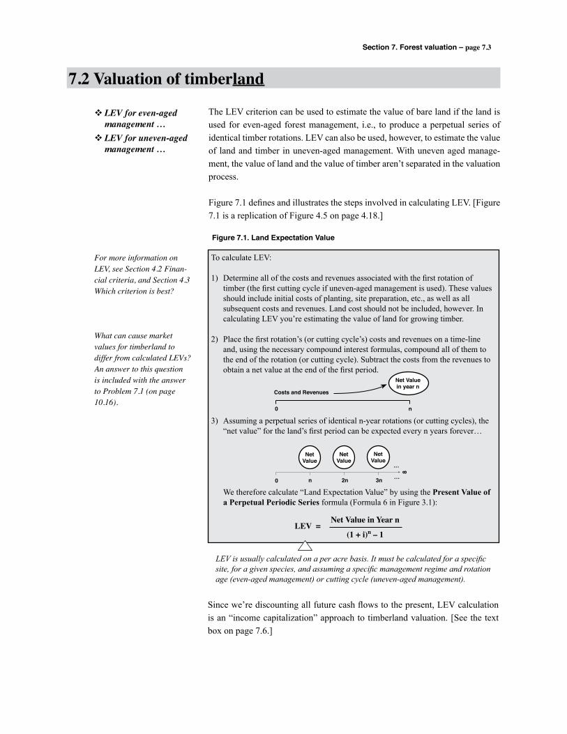
Section 7. Forest valuation – page 7.3
The LEV criterion can be used to estimate the value of bare land if the land is used for even-aged forest management, i.e., to produce a perpetual series of identical timber rotations. LEV can also be used, however, to estimate the value of land and timber in uneven-aged management. With uneven aged manage-ment, the value of land and the value of timber aren’t separated in the valuation process.
Figure 7.1 defines and illustrates the steps involved in calculating LEV. [Figure 7.1 is a replication of Figure 4.5 on page 4.18.]
7.2 Valuation of timberland
v LEV for even-aged management …v LEV for uneven-aged management …
Figure 7.1. Land Expectation Value
To calculate LEV:
1) Determine all of the costs and revenues associated with the first rotation of timber (the first cutting cycle if uneven-aged management is used). These values should include initial costs of planting, site preparation, etc., as well as all subsequent costs and revenues. Land cost should not be included, however. In calculating LEV you’re estimating the value of land for growing timber.
2) Place the first rotation’s (or cutting cycle’s) costs and revenues on a time-line and, using the necessary compound interest formulas, compound all of them to the end of the rotation (or cutting cycle). Subtract the costs from the revenues to obtain a net value at the end of the first period.
3) Assuming a perpetual series of identical n-year rotations (or cutting cycles), the “net value” for the land’s first period can be expected every n years forever…
We therefore calculate “Land Expectation Value” by using the Present Value of a Perpetual Periodic Series formula (Formula 6 in Figure 3.1):
LEV =Net Value in Year n
(1 + i)n – 1
LEV is usually calculated on a per acre basis. It must be calculated for a specific site, for a given species, and assuming a specific management regime and rotation age (even-aged management) or cutting cycle (uneven-aged management).
Costs and Revenues
0 n
Net Valuein year n
0 n
NetValue
3n2n …
NetValue
NetValue
…
8
Since we’re discounting all future cash flows to the present, LEV calculation is an “income capitalization” approach to timberland valuation. [See the text box on page 7.6.]
For more information on LEV, see Section 4.2 Finan-cial criteria, and Section 4.3 Which criterion is best?
What can cause market values for timberland to differ from calculated LEVs? An answer to this question is included with the answer to Problem 7.1 (on page 10.16).
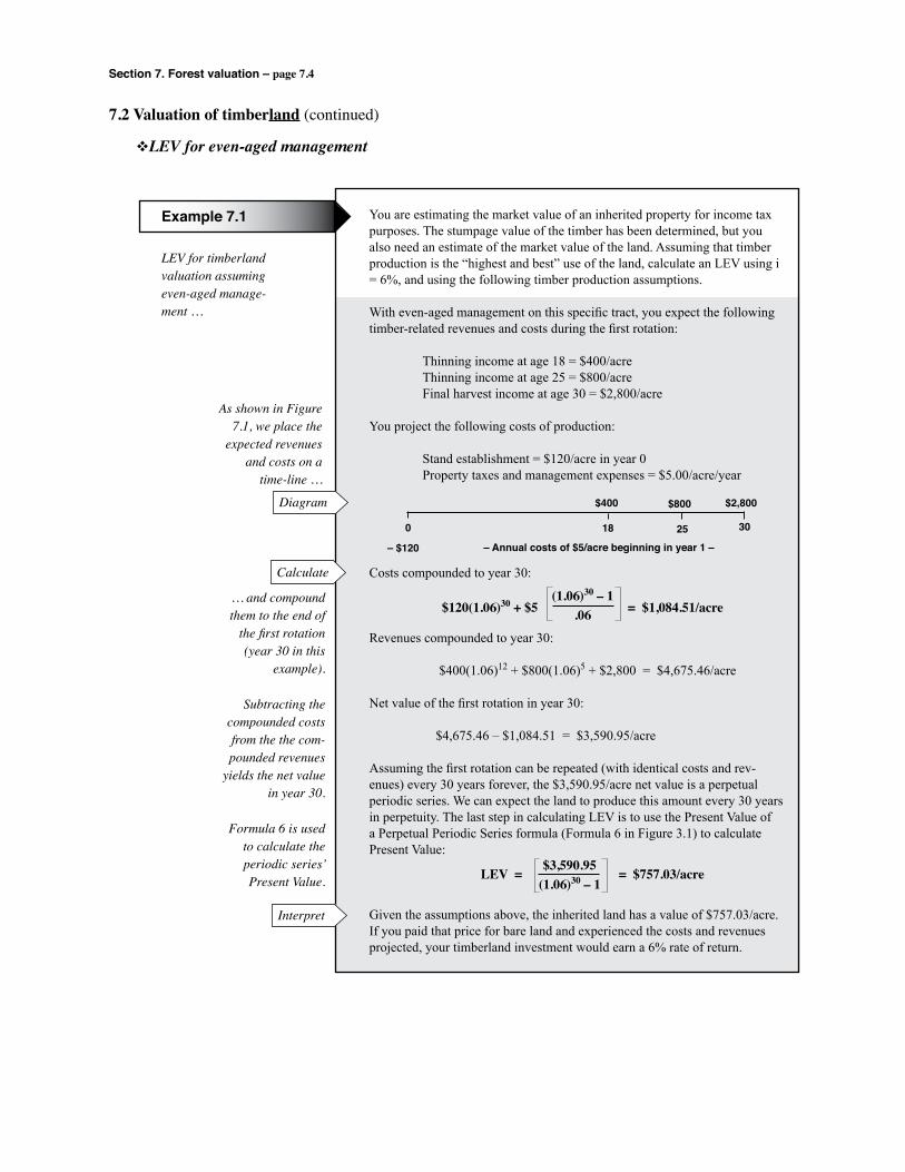
Section 7. Forest valuation – page 7.4
7.2 Valuation of timberland (continued)
vLEV for even-aged management
LEV for timberland valuation assuming even-aged manage-ment …
Example 7.1 You are estimating the market value of an inherited property for income tax purposes. The stumpage value of the timber has been determined, but you also need an estimate of the market value of the land. Assuming that timber production is the “highest and best” use of the land, calculate an LEV using i = 6%, and using the following timber production assumptions.
With even-aged management on this specific tract, you expect the following timber-related revenues and costs during the first rotation:
Thinning income at age 18 = $400/acre Thinning income at age 25 = $800/acre Final harvest income at age 30 = $2,800/acre
You project the following costs of production:
Stand establishment = $120/acre in year 0 Property taxes and management expenses = $5.00/acre/year
Costs compounded to year 30:
Revenues compounded to year 30:
$400(1.06)12 + $800(1.06)5 + $2,800 = $4,675.46/acre
Net value of the first rotation in year 30:
$4,675.46 – $1,084.51 = $3,590.95/acre
Assuming the first rotation can be repeated (with identical costs and rev-enues) every 30 years forever, the $3,590.95/acre net value is a perpetual periodic series. We can expect the land to produce this amount every 30 years in perpetuity. The last step in calculating LEV is to use the Present Value of a Perpetual Periodic Series formula (Formula 6 in Figure 3.1) to calculate Present Value:
Given the assumptions above, the inherited land has a value of $757.03/acre. If you paid that price for bare land and experienced the costs and revenues projected, your timberland investment would earn a 6% rate of return.
… and compound them to the end of
the first rotation (year 30 in this
example).
Subtracting the compounded costs from the the com-pounded revenues
yields the net value in year 30.
Formula 6 is used to calculate the periodic series’ Present Value.
As shown in Figure 7.1, we place the
expected revenues and costs on a
time-line …
0 18
$400
25
$800
30
$2,800
– $120 – Annual costs of $5/acre beginning in year 1 –
(1.06)30 – 1.06$120(1.06)30 + $5 = $1,084.51/acre
$3,590.95(1.06)30 – 1
LEV = = $757.03/acre
Diagram
Calculate
Interpret

Section 7. Forest valuation – page 7.5
7.2 Valuation of timberland (continued)
vLEV for even-aged management (continued)
LEV for lower site qualityland …
Problem 7.1 In Example 7.1, what if the LEV calculated applies to high site quality lands, but also in the inheritance were lands only capable of producing 75% of the high-site yields? What is the estimated market value of the lower site quality land? [Note that on lower site quality land, the highest LEV would probably result from using a management regime that’s different than the one projected for high-site land. For this problem, however, assume the same rotation length, thinning schedule, etc., that was used in Example 7.1.]
(Answer = $550.61/acre, as shown on page 10.16.)
0 18
$300
25
$600
30
$2,100
– $120
For this Problem, the revenues are 75% of those shown in Example 7.1.
– Annual costs of $5/acre beginning in year 1 –
LEV estimates are sensitive to all of the assumptions used in the calculations. These assumptions include prices, yields, costs, and the interest rate. For a discussion of these and other factors that affect LEV estimates, see page 4.19.
Diagram
Calculate
Interpret

Section 7. Forest valuation – page 7.6
7.2 Valuation of timberland (continued)
vLEV for even-aged management (continued)
Real estate appraisers typically use three approaches in estimating property values: cost-less-depreciation, comparable sales, and income capitalization (Smith and Corgel 1992).
How relevant are these approaches to estimating the value of forest-based assets?
n Cost-less-depreciation Timber and timberland don’t depreciate over time, so this valuation approach is not applicable in forest
valuation.
n Comparable sales (or “Transactions evidence”) The comparable sales approach to estimating timberland value is considered reliable, and this method
is generally preferred by the IRS for establishing a forested property’s basis for deduction (Siegel 1997). In many cases, however, information isn’t available on recent sales that are truly comparable to a specific forest property. Compared to other types of real property, timberland transactions are relatively infrequent, and land and timber price information isn’t available for many transactions that occur. Perhaps the biggest factor that limits the usefulness of the comparable sales approach in timber and timberland valuation, however, is finding sales that are truly comparable. Timber prices change seasonally due to weather and accessibility, and they can change dramatically in a short time due to shifts in supply and/or demand. Also affecting comparability of specific sales is the fact that many variables impact the value to buyers of a specific tract of timber and/or timberland at a given time. Land value, for example, is affected by potential productivity and operability, while standing timber values are affected by species, volume, and other characteristics that are highly variable from tract to tract.
The comparable sales approach is sometimes used to estimate the value of forest resources other than stumpage. For example, in Chapter 47. Appraising Forest Resource Value, Duerr (1993) cites reports that use the comparable sales approach in appraising urban forests and trees (Anderson and Cordell 1985), forested views from urban residential lots (Magill and Schwargz 1989), and water (Brown 1982).
n Income capitalization Income capitalization techniques can be used to estimate the value of most timber and timberland
assets. Techniques that use LEV or other discounted cash flow criteria to estimate the value of land and timber, for example, are simply means of discounting all future net income to the present using compound interest to account for the time value of projected costs and revenues. As a concept, LEV was developed by a German appraiser, Martin Faustmann (1849), to estimate the value of bare land for use in timber production.
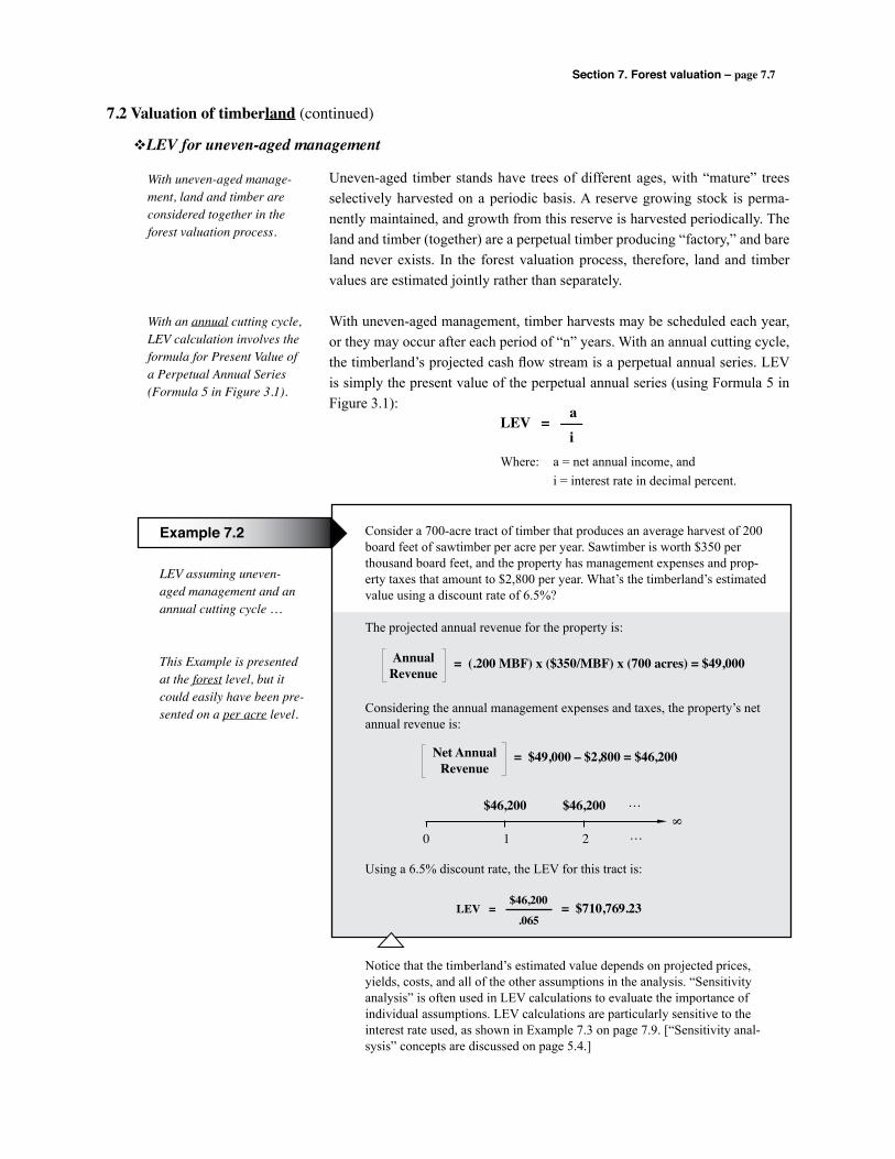
Section 7. Forest valuation – page 7.7
LEV assuming uneven-aged management and an annual cutting cycle …
This Example is presented at the forest level, but it could easily have been pre-sented on a per acre level.
Example 7.2 Consider a 700-acre tract of timber that produces an average harvest of 200 board feet of sawtimber per acre per year. Sawtimber is worth $350 per thousand board feet, and the property has management expenses and prop-erty taxes that amount to $2,800 per year. What’s the timberland’s estimated value using a discount rate of 6.5%?
The projected annual revenue for the property is:
Considering the annual management expenses and taxes, the property’s net annual revenue is:
Using a 6.5% discount rate, the LEV for this tract is:
Notice that the timberland’s estimated value depends on projected prices, yields, costs, and all of the other assumptions in the analysis. “Sensitivity analysis” is often used in LEV calculations to evaluate the importance of individual assumptions. LEV calculations are particularly sensitive to the interest rate used, as shown in Example 7.3 on page 7.9. [“Sensitivity anal-sysis” concepts are discussed on page 5.4.]
LEV = = $710,769.23 $46,200
.065
7.2 Valuation of timberland (continued)
vLEV for uneven-aged management
Uneven-aged timber stands have trees of different ages, with “mature” trees selectively harvested on a periodic basis. A reserve growing stock is perma-nently maintained, and growth from this reserve is harvested periodically. The land and timber (together) are a perpetual timber producing “factory,” and bare land never exists. In the forest valuation process, therefore, land and timber values are estimated jointly rather than separately.
With uneven-aged management, timber harvests may be scheduled each year, or they may occur after each period of “n” years. With an annual cutting cycle, the timberland’s projected cash flow stream is a perpetual annual series. LEV is simply the present value of the perpetual annual series (using Formula 5 in Figure 3.1):
With uneven-aged manage-ment, land and timber are considered together in the forest valuation process.
With an annual cutting cycle, LEV calculation involves the formula for Present Value of a Perpetual Annual Series (Formula 5 in Figure 3.1).
LEV = –––a
iWhere: a = net annual income, and i = interest rate in decimal percent.
= (.200 MBF) x ($350/MBF) x (700 acres) = $49,000AnnualRevenue
= $49,000 – $2,800 = $46,200Net AnnualRevenue
0 1 2
$46,200 $46,200
8
…
…
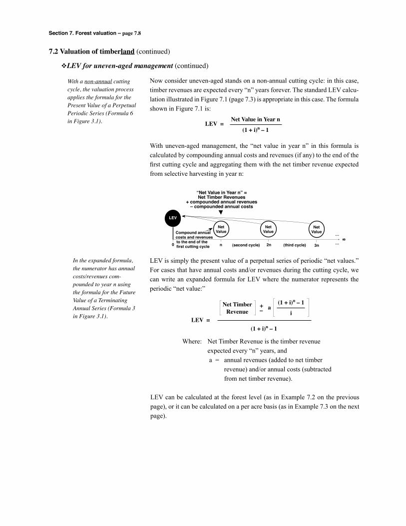
Section 7. Forest valuation – page 7.8
In the expanded formula, the numerator has annual costs/revenues com-pounded to year n using the formula for the Future Value of a Terminating Annual Series (Formula 3 in Figure 3.1).
7.2 Valuation of timberland (continued)
vLEV for uneven-aged management (continued)
Now consider uneven-aged stands on a non-annual cutting cycle: in this case, timber revenues are expected every “n” years forever. The standard LEV calcu-lation illustrated in Figure 7.1 (page 7.3) is appropriate in this case. The formula shown in Figure 7.1 is:
With uneven-aged management, the “net value in year n” in this formula is calculated by compounding annual costs and revenues (if any) to the end of the first cutting cycle and aggregating them with the net timber revenue expected from selective harvesting in year n:
With a non-annual cutting cycle, the valuation process applies the formula for the Present Value of a Perpetual Periodic Series (Formula 6 in Figure 3.1). LEV =
Net Value in Year n
(1 + i)n – 1
LEV is simply the present value of a perpetual series of periodic “net values.” For cases that have annual costs and/or revenues during the cutting cycle, we can write an expanded formula for LEV where the numerator represents the periodic “net value:”
LEV =
Net TimberRevenue
+– a
(1 + i)n – 1
i
(1 + i)n – 1
Where: Net Timber Revenue is the timber revenue expected every “n” years, and a = annual revenues (added to net timber revenue) and/or annual costs (subtracted from net timber revenue).
LEV can be calculated at the forest level (as in Example 7.2 on the previous page), or it can be calculated on a per acre basis (as in Example 7.3 on the next page).
0 n 3n2n
NetValue
NetValue
…
…
8
(second cycle) (third cycle)
LEV
Compound annualcosts and revenuesto the end of thefirst cutting cycle
“Net Value in Year n” =Net Timber Revenues
+ compounded annual revenues– compounded annual costs
NetValue

Section 7. Forest valuation – page 7.9
LEV for timberland valuation assum-ing uneven-aged management and a non-annual cutting cycle …
Example 7.3 Consider a 2,000 acre forest that produces $350 of net timber revenue per acre every five years (beginning five years from now). Annual management fees and property taxes are $3.00 per acre per year, and there’s a hunting lease that provides an income of $5.00 per acre per year. What’s the timberland’s estimated value using a discount rate of 7%?
Since the $5 per year income series and the $3 per year cost series occur throughout the time-line, we can save effort in this Example by using
$5 – $3 = $2 as the net annual income per acre per year.
The expanded formula on page 7.8 can be used to calculate LEV using $2 as a net revenue each year:
The estimated value of the timberland is $898.02 per acre. As stated with earlier Examples, this estimate is sensitive to all of the cost and revenue assumptions, as well as the discount rate used in the analysis.
Listed below are LEV estimates for this Example using different discount rates …
Notice that the timberland’s estimated value decreases as the discount rate is increased. When we increase the discount rate we’re discounting future net revenues to the present at a higher rate, so they’re smaller in present value terms.
LEV estimates are sensitive to the
assumptions used in the analysis.
The discount rate used is extremely
important.
Diagram
Calculate
Interpret
7.2 Valuation of timberland (continued)
vLEV for uneven-aged management (continued)
0 1 2 3 4 5
$5 $5 $5 $5 $5
-$3 -$3 -$3 -$3 -$3
$350 We assume that this revenue/cost stream will be repeated every five years in perpetuity.
LEV =
$350 + $2(1.07)5 – 1
.07
(1.07)5 – 1= $898.02/acre
DiscountRate
Estimated Timberland Value(LEV per acre)
3%
5%
7%
9%
11%
$2,264.14
$1,306.82
$898.02
$672.03
$529.09
Section 7. Forest valuation – page 7.10
7.2 Valuation of timberland (continued)
vLEV for uneven-aged management (continued)
LEV for timberland in uneven-aged management with a non-annual cutting cycle …
Problem 7.2 What’s the estimated value per acre of an uneven-aged forest given the follow-ing assumptions? Cutting cycle = 10 years Annual cost = $9/acre Projected net timber revenue = $600 every 10 years Discount rate = 8% The next harvest is 10 years from now.(Answer = $405.22/acre, as shown on page 10.17.)
Diagram
Calculate
Interpret
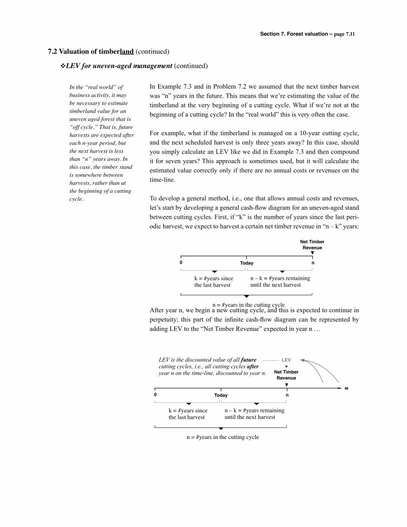
Section 7. Forest valuation – page 7.11
7.2 Valuation of timberland (continued)
vLEV for uneven-aged management (continued)
In Example 7.3 and in Problem 7.2 we assumed that the next timber harvest was “n” years in the future. This means that we’re estimating the value of the timberland at the very beginning of a cutting cycle. What if we’re not at the beginning of a cutting cycle? In the “real world” this is very often the case.
For example, what if the timberland is managed on a 10-year cutting cycle, and the next scheduled harvest is only three years away? In this case, should you simply calculate an LEV like we did in Example 7.3 and then compound it for seven years? This approach is sometimes used, but it will calculate the estimated value correctly only if there are no annual costs or revenues on the time-line.
To develop a general method, i.e., one that allows annual costs and revenues, let’s start by developing a general cash-flow diagram for an uneven-aged stand between cutting cycles. First, if “k” is the number of years since the last peri-odic harvest, we expect to harvest a certain net timber revenue in “n – k” years:
After year n, we begin a new cutting cycle, and this is expected to continue in perpetuity; this part of the infinite cash-flow diagram can be represented by adding LEV to the “Net Timber Revenue” expected in year n …
In the “real world” of business activity, it may be necessary to estimate timberland value for an uneven aged forest that is “off cycle.” That is, future harvests are expected after each n-year period, but the next harvest is less than “n” years away. In this case, the timber stand is somewhere between harvests, rather than at the beginning of a cutting cycle.
Today0 n
Net TimberRevenue
k = #years sincethe last harvest
n – k = #years remaininguntil the next harvest
n = #years in the cutting cycle
Today0 n
LEV+
Net TimberRevenue
k = #years sincethe last harvest
n – k = #years remaininguntil the next harvest
n = #years in the cutting cycle
LEV is the discounted value of all futurecutting cycles, i.e., all cutting cycles afteryear n on the time-line, discounted to year n.
8
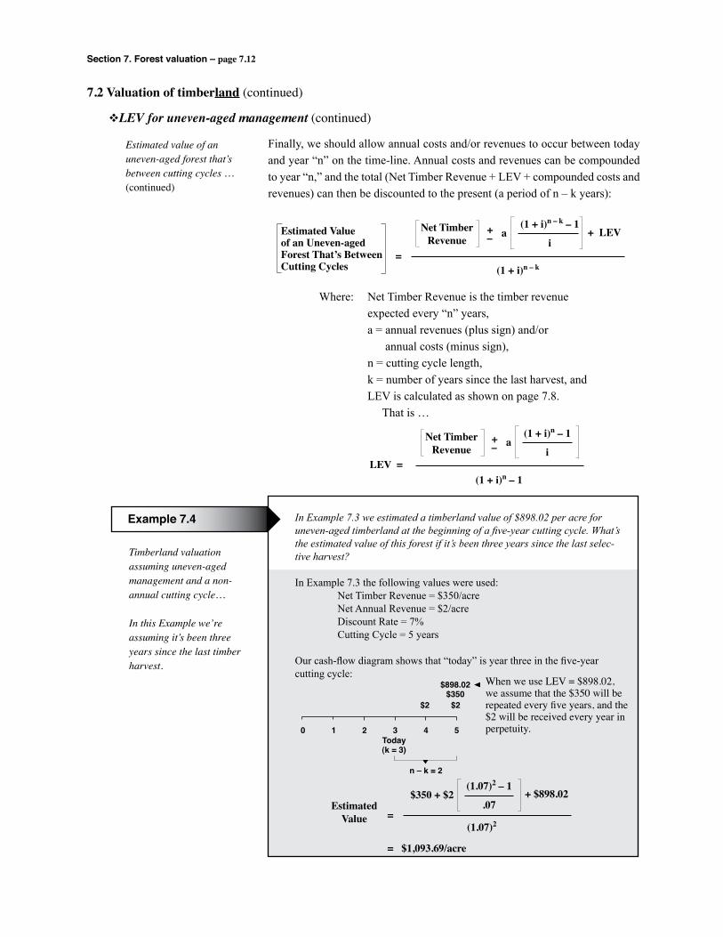
Section 7. Forest valuation – page 7.12
Timberland valuation assuming uneven-aged management and a non-annual cutting cycle…
In this Example we’re assuming it’s been three years since the last timber harvest.
In Example 7.3 we estimated a timberland value of $898.02 per acre for uneven-aged timberland at the beginning of a five-year cutting cycle. What’s the estimated value of this forest if it’s been three years since the last selec-tive harvest?
In Example 7.3 the following values were used: Net Timber Revenue = $350/acre Net Annual Revenue = $2/acre Discount Rate = 7% Cutting Cycle = 5 years
Our cash-flow diagram shows that “today” is year three in the five-yearcutting cycle:
Example 7.4
7.2 Valuation of timberland (continued)
vLEV for uneven-aged management (continued)
Finally, we should allow annual costs and/or revenues to occur between today and year “n” on the time-line. Annual costs and revenues can be compounded to year “n,” and the total (Net Timber Revenue + LEV + compounded costs and revenues) can then be discounted to the present (a period of n – k years):
Estimated value of an uneven-aged forest that’s between cutting cycles …(continued)
LEV =
Net TimberRevenue
+– a
(1 + i)n – 1
i
(1 + i)n – 1
Net TimberRevenue
+– a
(1 + i)n – k – 1
i
(1 + i)n – k
Estimated Valueof an Uneven-agedForest That’s BetweenCutting Cycles
=
+ LEV
Where: Net Timber Revenue is the timber revenue expected every “n” years, a = annual revenues (plus sign) and/or annual costs (minus sign), n = cutting cycle length, k = number of years since the last harvest, and LEV is calculated as shown on page 7.8. That is …
When we use LEV = $898.02, we assume that the $350 will be repeated every five years, and the $2 will be received every year in perpetuity.0 1 2 3 4 5
$2 $2
$898.02$350
Today(k = 3)
n – k = 2
EstimatedValue
(1.07)2
$350 + $2(1.07)2 – 1
.07+ $898.02
=
= $1,093.69/acre
Section 7. Forest valuation – page 7.13
Estimated value of timberland in uneven-aged management, assuming the stand is in year six of a 10-year cutting cycle …
Problem 7.3 What’s the estimated value per acre of an uneven-aged forest given the follow-ing assumptions? Cutting cycle = 10 years Annual revenue = $12/acre; Annual cost = $4/acre Projected net timber revenue = $750 every 10 years Discount rate = 9% The next harvest is 4 years from now.(Answer = $1,008.78/acre, as shown on page 10.17.)
The error from not using the general formula on page 7.12 can be significant.
7.2 Valuation of timberland (continued)
vLEV for uneven-aged management (continued)
In Example 7.4, the estimated timberland value is $1,093.69/acre, and note that this is not the same as simply compounding LEV for three years:
$898.02(1.07)3 = $1,100.11/acre
The error ($6.42 in this Example) occurs because compounding LEV in Exam-ple 7.4 would assume that the annual revenues of $2 that occurred in year 1, year 2, and year 3 of the present cutting cycle are relevant to the forest’s value today. Notice in the cash-flow diagram in Example 7.4 that there are no reve-nues above these years on the time-line; they occurred before today and should therefore not be considered in the forest valuation process.
In Example 7.4 the error from estimating timberland value by calculating LEV and compounding it for three years is relatively small ($6.42/acre). In many “real world” cases, however, the error can be significant. For example, in an analysis involving a forest that’s in year eight of a 10 year cutting cycle, with $10/acre annual revenues and using i = 8%, simply compounding LEV to year eight would result in an estimated forest value that’s $106.37/acre too high.
As stated on page 7.11, compounding LEV for an “off-cycle” uneven-aged will yield the correct estimated value only if the time line has no annual costs or revenues.

Section 7. Forest valuation – page 7.14
Foresters are frequently called on to estimate the value of standing timber. In many cases, of course, the timber’s value must be estimated because it’s being offered for sale.
In other cases, a market value estimate is needed even though the timber isn’t for sale. Timberland that’s inherited, for example, must be divided into a land account and a timber account for income tax purposes. Estimating these values establishes the land’s basis for deduction and the timber’s basis for depletion (as discussed in Section 6.2 Income taxes). These account values are to be based on the estimated market value of the timber and the estimated market value of the land at the time the timberland was acquired.
If you’re estimating the value of standing timber whose size or age is appro-priate for harvest, the time value of money isn’t a factor in the valuation process. The merchantable timber’s value can be estimated as a “liquidation value,” without discounting future revenues to the present. If you’re estimat-ing the value of timber stands that are precommercial, however, or timber that could be sold but hasn’t yet reached the size or age where harvest is planned, a valuation process is needed that accounts for the time value of money.
Section 7.3 therefore has two subsections:
v Liquidation value of timber and v Valuation of immature timber.
“Liquidation value” is the estimated amount of money that would be received for immediate sale of an asset (Klemperer 1987). For standing timber, liqui-dation value is the stumpage value for immediate harvest. In this definition, note that the word “immediate” is relative. This subsection is a very brief discussion of the process of estimating the stumpage value of timber that will be “liquidated” or harvested “relatively soon.” How soon? “Relatively soon” simply means soon enough that the time value of money doesn’t need to be considered in estimating the timber’s harvest value today.
Liquidation value also applies to timber stands that aren’t currently scheduled for harvest, but whose value must be estimated for establishing their basis for depletion. In this case, the market value of merchantable timber is “liquida-tion value of the trees on the date of valuation rather than the timber’s poten-tial value at some future time” (Siegel 1997).
7.3 Valuation of standing timber
Section 7.3 includes basic concepts and approaches for estimating the value of standing timber. The pro-cess of marketing standing timber isn’t covered here, but references on timber marketing are included in Section 7.6. References on forest valuation.
v Liquidation value of timber
The words “standing timber” and “stumpage” are used synonymously in this discussion.
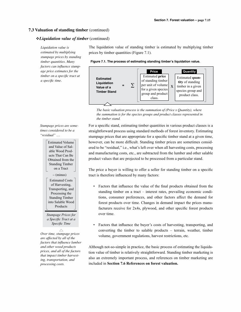
Section 7. Forest valuation – page 7.15
7.3 Valuation of standing timber (continued)
vLiquidation value of timber (continued)
The liquidation value of standing timber is estimated by multiplying timber prices by timber quantities (Figure 7.1).
Figure 7.1. The process of estimating standing timber’s liquidation value.
Liquidation value is estimated by multiplying stumpage prices by standing timber quantities. Many factors can influence stump-age price estimates for the timber on a specific tract at a specific time.
The basic valuation process is the summation of (Price x Quantity), where the summation is for the species groups and product classes represented in the timber stand.
Estimated price of standing timber per unit of volume for a given species group and product
class.
Estimated quan-tity of standing
timber in a given species group and
product class.
EstimatedLiquidationValue of a Timber Stand
= ∑ x
Price Quantity
For a specific stand, estimating timber quantities in various product classes is a straightforward process using standard methods of forest inventory. Estimating stumpage prices that are appropriate for a specific timber stand at a given time, however, can be more difficult. Standing timber prices are sometimes consid-ered to be “residual,” i.e., what’s left over when all harvesting costs, processing and manufacturing costs, etc., are subtracted from the lumber and other salable product values that are projected to be processed from a particular stand.
The price a buyer is willing to offer a seller for standing timber on a specific tract is therefore influenced by many factors:
• Factors that influence the value of the final products obtained from the standing timber on a tract – interest rates, prevailing economic condi-tions, consumer preferences, and other factors affect the demand for forest products over time. Changes in demand impact the prices manu-facturers receive for 2x4s, plywood, and other specific forest products over time.
• Factors that influence the buyer’s costs of harvesting, transporting, and
converting the timber to salable products – terrain, weather, timber volume, government regulations, harvest restrictions, etc.
Although not-so-simple in practice, the basic process of estimating the liquida-tion value of timber is relatively straightforward. Standing timber marketing is also an extremely important process, and references on timber marketing are included in Section 7.6 References on forest valuation.
Stumpage prices are some-times considered to be a “residual” …
Over time, stumpage prices are affected by all of the factors that influence lumber and other wood products prices, and all of the factors that impact timber harvest-ing, transportation, and processing costs.
Estimated Volume and Value of Sal-able Wood Prod-ucts That Can Be Obtained from the Standing Timber
on a Tract
Estimated Costs of Harvesting,
Transporting, and Processing the
Standing Timber into Salable Wood
Products
– (minus)
Stumpage Prices for a Specific Tract at a
Specific Time
Section 7. Forest valuation – page 7.16
7.3 Valuation of standing timber (continued)
vValuation of immature timber
Two methods are often used to estimate the value of precommercial timber. [See Foster (1986a) in the list of references on page 7.21.]
• “Buyer’s value” is based on discounting all of the projected timber sale revenues to the present, often using the current market interest rate or an estimate of expected interest rates over the projection period. This value represents the maximum a buyer would be willing to pay for a precommercial stand of timber.
• “Seller’s value” is based on compounding all production costs at a speci-fied interest rate, usually the historical market rate over the time period involved. This represents a minimum value for the seller, i.e., the seller would accept no less than this compounded value.
Obviously, when compounding or discounting over the long time periods involved in many forestry investments, the choice of an interest rate is crucial to the valuation process. In many cases, buyer’s and seller’s values are deter-mined using different interest rates, but even if the same interest rate is used, inconsistent results may occur.
As will be discussed, if the interest rate used for immature stand valuation is the internal rate of return (ROR) of the timber investment, the buyer’s value will equal the seller’s value at every stand age.
Listed below is a typical cash flow generated by a southern pine plantation:
This subsection will show that a precommercial timber stand represents more than compounded out of-pocket costs or discounted timber harvest revenues; immature timber stands will be undervalued if land opportunity cost is ignored.
Year
0
1–25
1–25
25
Item
Site Prep/Planting
Annual Property Taxand Management Fee
Annual Hunting Lease
Net Harvest Revenue
Cash Flow Per Acre
– $150.00
– $3.50
+ $3.50
+ $2,550.00
In this subsection, valua-tion of immature timber is presented by developing an example application for a 12 year-old southern pine plantation.
Here we assume that annual expenses equal annual revenues (a reasonable assumption that doesn’t affect the analysis). Also, intermediate costs and inter-mediate harvest revenues are not projected; this allows us to use simple graph-ics, but doesn’t impact the analytical results.
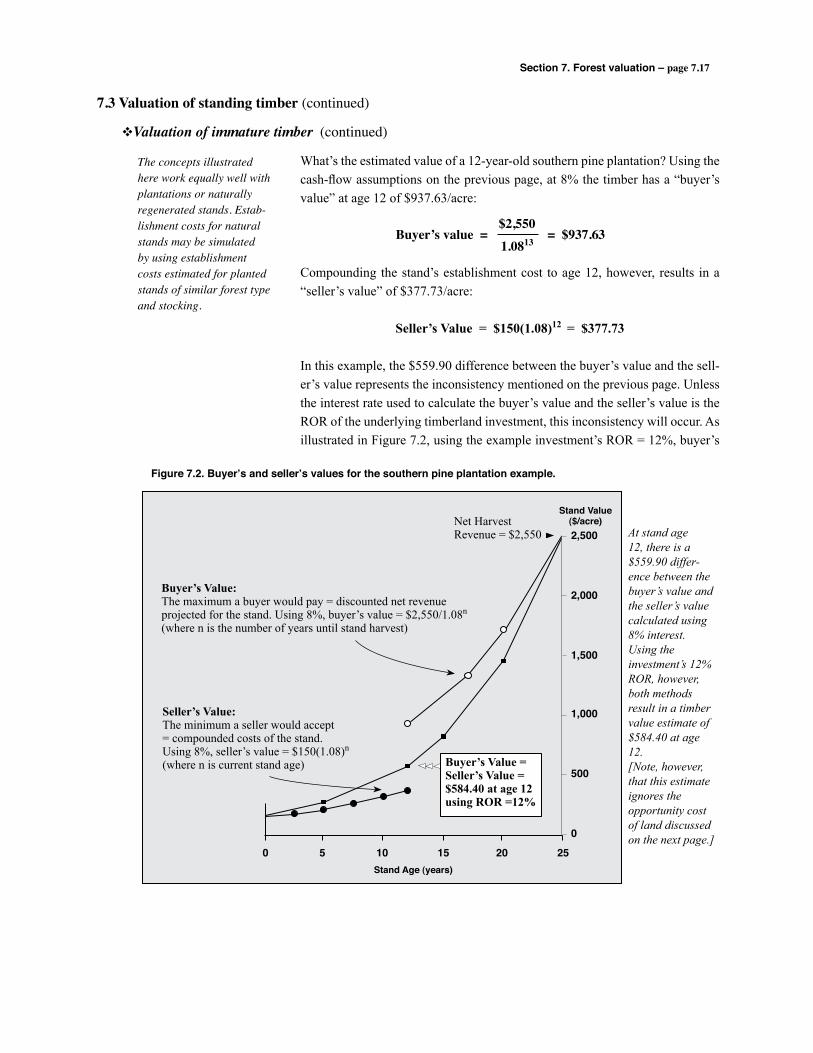
Section 7. Forest valuation – page 7.17
7.3 Valuation of standing timber (continued)
vValuation of immature timber (continued)
What’s the estimated value of a 12-year-old southern pine plantation? Using the cash-flow assumptions on the previous page, at 8% the timber has a “buyer’s value” at age 12 of $937.63/acre:
Compounding the stand’s establishment cost to age 12, however, results in a “seller’s value” of $377.73/acre:
Seller’s Value = $150(1.08)12 = $377.73
In this example, the $559.90 difference between the buyer’s value and the sell-er’s value represents the inconsistency mentioned on the previous page. Unless the interest rate used to calculate the buyer’s value and the seller’s value is the ROR of the underlying timberland investment, this inconsistency will occur. As illustrated in Figure 7.2, using the example investment’s ROR = 12%, buyer’s
The concepts illustrated here work equally well with plantations or naturally regenerated stands. Estab-lishment costs for natural stands may be simulated by using establishment costs estimated for planted stands of similar forest type and stocking.
Buyer’s value = = $937.63$2,550
1.0813
0 5 10 15 20 25
2,500
2,000
1,500
1,000
500
0
Net HarvestRevenue = $2,550
Buyer’s Value:The maximum a buyer would pay = discounted net revenueprojected for the stand. Using 8%, buyer’s value = $2,550/1.08n
(where n is the number of years until stand harvest)
Seller’s Value:The minimum a seller would accept = compounded costs of the stand.Using 8%, seller’s value = $150(1.08)n
(where n is current stand age)
At stand age 12, there is a $559.90 differ-ence between the buyer’s value and the seller’s value calculated using 8% interest. Using the investment’s 12% ROR, however, both methods result in a timber value estimate of $584.40 at age 12. [Note, however, that this estimate ignores the opportunity cost of land discussed on the next page.]
Buyer’s Value =Seller’s Value = $584.40 at age 12using ROR =12%
Stand Age (years)
Stand Value($/acre)
Figure 7.2. Buyer’s and seller’s values for the southern pine plantation example.
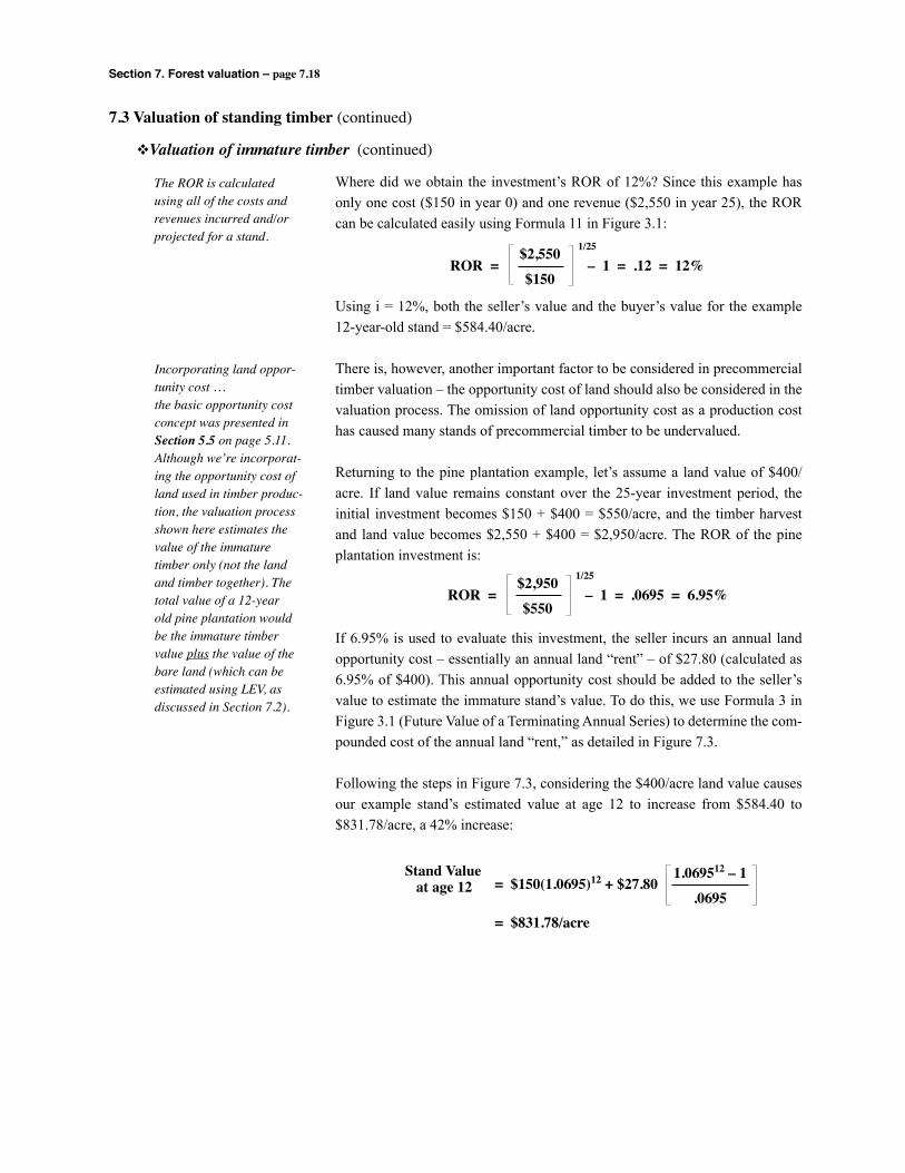
Section 7. Forest valuation – page 7.18
7.3 Valuation of standing timber (continued)
vValuation of immature timber (continued)
Where did we obtain the investment’s ROR of 12%? Since this example has only one cost ($150 in year 0) and one revenue ($2,550 in year 25), the ROR can be calculated easily using Formula 11 in Figure 3.1:
Using i = 12%, both the seller’s value and the buyer’s value for the example 12-year-old stand = $584.40/acre.
There is, however, another important factor to be considered in precommercial timber valuation – the opportunity cost of land should also be considered in the valuation process. The omission of land opportunity cost as a production cost has caused many stands of precommercial timber to be undervalued.
Returning to the pine plantation example, let’s assume a land value of $400/acre. If land value remains constant over the 25-year investment period, the initial investment becomes $150 + $400 = $550/acre, and the timber harvest and land value becomes $2,550 + $400 = $2,950/acre. The ROR of the pine plantation investment is:
If 6.95% is used to evaluate this investment, the seller incurs an annual land opportunity cost – essentially an annual land “rent” – of $27.80 (calculated as 6.95% of $400). This annual opportunity cost should be added to the seller’s value to estimate the immature stand’s value. To do this, we use Formula 3 in Figure 3.1 (Future Value of a Terminating Annual Series) to determine the com-pounded cost of the annual land “rent,” as detailed in Figure 7.3.
Following the steps in Figure 7.3, considering the $400/acre land value causes our example stand’s estimated value at age 12 to increase from $584.40 to $831.78/acre, a 42% increase:
The ROR is calculated using all of the costs and revenues incurred and/or projected for a stand.
ROR = – 1 = .12 = 12%$2,550
$150
1/25
ROR = – 1 = .0695 = 6.95%$2,950
$550
1/25
Stand Value at age 12
1.069512 – 1
.0695= $150(1.0695)12 + $27.80
= $831.78/acre
Incorporating land oppor-tunity cost …the basic opportunity cost concept was presented in Section 5.5 on page 5.11. Although we’re incorporat-ing the opportunity cost of land used in timber produc-tion, the valuation process shown here estimates the value of the immature timber only (not the land and timber together). The total value of a 12-year old pine plantation would be the immature timber value plus the value of the bare land (which can be estimated using LEV, as discussed in Section 7.2).
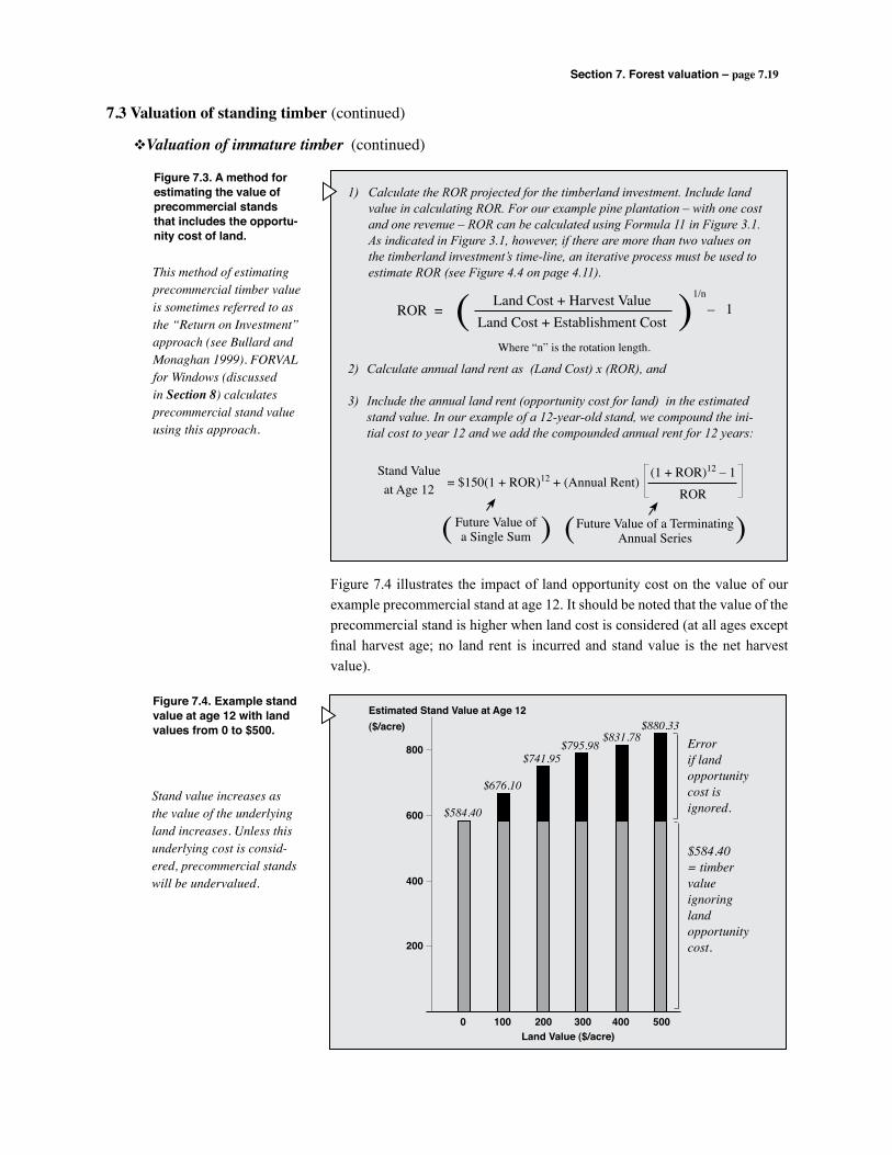
Section 7. Forest valuation – page 7.19
7.3 Valuation of standing timber (continued)
vValuation of immature timber (continued)
Figure 7.3. A method for estimating the value of precommercial stands that includes the opportu-nity cost of land.
1) Calculate the ROR projected for the timberland investment. Include land value in calculating ROR. For our example pine plantation – with one cost and one revenue – ROR can be calculated using Formula 11 in Figure 3.1. As indicated in Figure 3.1, however, if there are more than two values on the timberland investment’s time-line, an iterative process must be used to estimate ROR (see Figure 4.4 on page 4.11).
2) Calculate annual land rent as (Land Cost) x (ROR), and
3) Include the annual land rent (opportunity cost for land) in the estimated stand value. In our example of a 12-year-old stand, we compound the ini-tial cost to year 12 and we add the compounded annual rent for 12 years:
ROR =Land Cost + Harvest Value
Land Cost + Establishment Cost
1/n( ) – 1
Stand Valueat Age 12 = $150(1 + ROR)12 + (Annual Rent)
(1 + ROR)12 – 1
ROR
Future Value ofa Single Sum( ) Future Value of a Terminating
Annual Series( )
This method of estimating precommercial timber value is sometimes referred to as the “Return on Investment” approach (see Bullard and Monaghan 1999). FORVAL for Windows (discussed in Section 8) calculates precommercial stand value using this approach.
Figure 7.4 illustrates the impact of land opportunity cost on the value of our example precommercial stand at age 12. It should be noted that the value of the precommercial stand is higher when land cost is considered (at all ages except final harvest age; no land rent is incurred and stand value is the net harvest value).
Figure 7.4. Example stand value at age 12 with land values from 0 to $500.
Stand value increases as the value of the underlying land increases. Unless this underlying cost is consid-ered, precommercial stands will be undervalued.
Errorif landopportunitycost isignored.
$584.40= timbervalueignoringlandopportunitycost.
$584.40
$676.10
$741.95$795.98
$831.78$880.33
0 100 200 300 400 500Land Value ($/acre)
Estimated Stand Value at Age 12($/acre)
200
400
600
800
Where “n” is the rotation length.

Section 7. Forest valuation – page 7.20
As a final part of this subsection on estimating the value of immature timber stands, there is a valuation approach that applies the LEV criterion. For an immature timber stand that meets the assumptions used to calculate LEV, a simple calculation can be used to estimate stand value:
Where Vm = Value of the m-aged timber stand, m = age of the immature stand, n = rotation length used in calculating LEV, and NV = Net Value of the income and costs associated with
the immature stand between year m and rotation age n.
As an example, assume you spent $125/acre on stand regeneration, and you project a thinning of $900/acre at stand age 20 and a final harvest value of $3,000/acre at stand age 30. Using a discount rate of 7%, what’s the estimated value of your 8-year-old stand?
The cash-flow diagram shows that our stand is in year eight of a projected 30-year rotation:
Using the LEV-based approach above, we first calculate LEV:
We then calculate “Net Value” in year 30 by compounding the projected costs and revenues between year 8 and year 30 to the end of the rotation. In this example, we only have revenues, and “Net Value” at year 30 is:
NV30 = $900(1.07)10 + $3,000 = $4,770.44
The estimated stand value at age eight is therefore:
For an explanation of why the LEV method “works,” see Figure 7.5.
7.3 Valuation of standing timber (continued)
vValuation of immature timber (continued)
NVn + LEV
(1 + i)n–mVm = – LEV
0 8 20 30
$900 $3,000
Today– $125
LEV =$3,000 + $900(1.07)10 – $125(1.07)30
(1.07)30 – 1= $577.55/acre
Stand Valueat Age 8
= – $577.55 = $629.56/acre$4,770.44 + $577.55
(1.07)22
[Note that the value of the land and timber in this example is: $577.55, the land value + $629.56, the timber value = $1,207.11.]
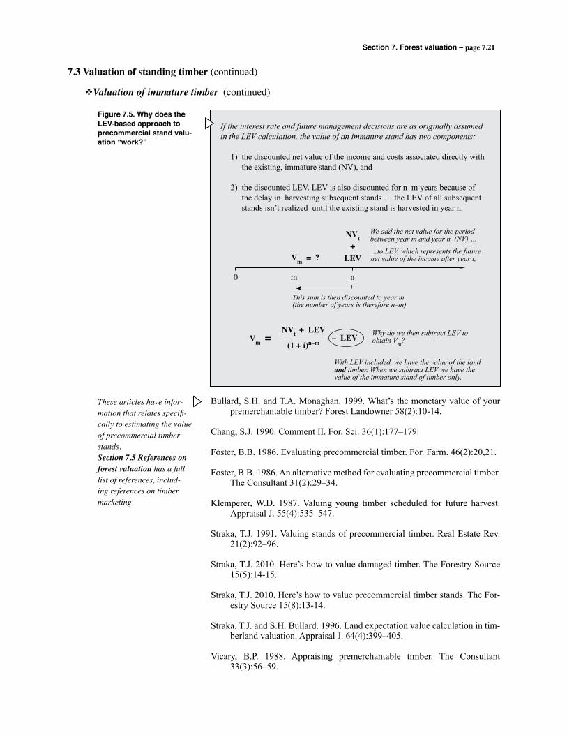
Section 7. Forest valuation – page 7.21
Figure 7.5. Why does the LEV-based approach to precommercial stand valu-ation “work?”
These articles have infor-mation that relates specifi-cally to estimating the value of precommercial timber stands. Section 7.5 References on forest valuation has a full list of references, includ-ing references on timber marketing.
7.3 Valuation of standing timber (continued)
vValuation of immature timber (continued)
If the interest rate and future management decisions are as originally assumed in the LEV calculation, the value of an immature stand has two components:
1) the discounted net value of the income and costs associated directly with the existing, immature stand (NV), and
2) the discounted LEV. LEV is also discounted for n–m years because of the delay in harvesting subsequent stands … the LEV of all subsequent stands isn’t realized until the existing stand is harvested in year n.
0 m n
Vm = ?
NVt+
LEV
We add the net value for the period between year m and year n (NV) …
…to LEV, which represents the future net value of the income after year t,
This sum is then discounted to year m (the number of years is therefore n–m).
Vm =NVt + LEV
(1 + i)n–m– LEV Why do we then subtract LEV to
obtain Vm?
With LEV included, we have the value of the land and timber. When we subtract LEV we have the value of the immature stand of timber only.
Bullard, S.H. and T.A. Monaghan. 1999. What’s the monetary value of your premerchantable timber? Forest Landowner 58(2):10-14.
Chang, S.J. 1990. Comment II. For. Sci. 36(1):177–179.
Foster, B.B. 1986. Evaluating precommercial timber. For. Farm. 46(2):20,21.
Foster, B.B. 1986. An alternative method for evaluating precommercial timber. The Consultant 31(2):29–34.
Klemperer, W.D. 1987. Valuing young timber scheduled for future harvest. Appraisal J. 55(4):535–547.
Straka, T.J. 1991. Valuing stands of precommercial timber. Real Estate Rev. 21(2):92–96.
Straka, T.J. 2010. Here’s how to value damaged timber. The Forestry Source 15(5):14-15.
Straka, T.J. 2010. Here’s how to value precommercial timber stands. The For-estry Source 15(8):13-14.
Straka, T.J. and S.H. Bullard. 1996. Land expectation value calculation in tim-berland valuation. Appraisal J. 64(4):399–405.
Vicary, B.P. 1988. Appraising premerchantable timber. The Consultant 33(3):56–59.
Section 7. Forest valuation – page 7.22
7.1 Introduction Foresters are often called on to estimate the market value of land and timber.
Section 7 is limited to valuation techniques that focus on the monetary value of forests used for commercial timber production.
7.2 Valuation of timberland
vLEVforeven-agedmanagement LEV can be used to estimate the value of bare land if the land is used for even-
aged forest management, i.e., to produce a perpetual series of identical timber rotations. Since all future cash flows are discounted to the present, LEV calcu-lation is an “income capitalization” approach to timberland valuation.
vLEVforuneven-agedmanagement With uneven-aged management, land and timber are a perpetual timber pro-
ducing “factory” and the land is never bare. In the forest valuation process, therefore, land and timber values are estimated jointly.
With an annual cutting cycle, the timberland’s projected cash-flow stream is a perpetual annual series. LEV is simply the present value of the perpetual annual series:
Where “a” is the net annual harvest value.
With a non-annual cutting cycle, timber revenues are projected every “n” years forever, and the standard LEV calculation is appropriate:
In this case, the “Net Value in Year n” is calculated by compounding annual costs and revenues (if any) to the end of the first cutting cycle and aggregating them with the net timber revenue expected from selection harvesting in year n. The formula can be expanded to include annual costs and revenues:
7.4 Review of Section 7
Section 7. Forest Valuation
LEV =a
i
LEV =Net Value in Year n
(1 + i)n – 1
LEV =
Net TimberRevenue
+– a
(1 + i)n – 1
i
(1 + i)n – 1
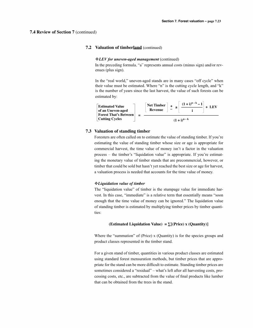
Section 7. Forest valuation – page 7.23
7.4 Review of Section 7 (continued)
7.2 Valuation of timberland (continued)
vLEVforuneven-agedmanagement(continued) In the preceding formula, “a” represents annual costs (minus sign) and/or rev-
enues (plus sign).
In the “real world,” uneven-aged stands are in many cases “off cycle” when their value must be estimated. Where “n” is the cutting cycle length, and “k” is the number of years since the last harvest, the value of such forests can be estimated by:
7.3 Valuation of standing timber Foresters are often called on to estimate the value of standing timber. If you’re
estimating the value of standing timber whose size or age is appropriate for commercial harvest, the time value of money isn’t a factor in the valuation process – the timber’s “liquidation value” is appropriate. If you’re estimat-ing the monetary value of timber stands that are precommercial, however, or timber that could be sold but hasn’t yet reached the best size or age for harvest, a valuation process is needed that accounts for the time value of money.
vLiquidation value of timber The “liquidation value” of timber is the stumpage value for immediate har-
vest. In this case, “immediate” is a relative term that essentially means “soon enough that the time value of money can be ignored.” The liquidation value of standing timber is estimated by multiplying timber prices by timber quanti-ties:
(Estimated Liquidation Value) = ∑[(Price) x (Quantity)]
Where the “summation” of (Price) x (Quantity) is for the species groups and product classes represented in the timber stand.
For a given stand of timber, quantities in various product classes are estimated using standard forest mensuration methods, but timber prices that are appro-priate for the stand can be more difficult to estimate. Standing timber prices are sometimes considered a “residual” – what’s left after all harvesting costs, pro-cessing costs, etc., are subtracted from the value of final products like lumber that can be obtained from the trees in the stand.
Net TimberRevenue
+– a
(1 + i)n – k – 1
i
(1 + i)n – k
Estimated Valueof an Uneven-agedForest That’s BetweenCutting Cycles
=
+ LEV

Section 7. Forest valuation – page 7.24
7.4 Review of Section 7 (continued)
7.2 Valuation of standing timber (continued)
vLiquidationvalueoftimber(continued) The price a timber buyer is willing to pay for the standing timber on a specific
tract at a specific time is influenced by many factors – those that affect the value of the final products, and those that affect the buyer’s costs of harvesting, transporting, and processing the timber. Section 7 doesn’t include a formal dis-cussion of timber marketing, but references on timber marketing are included in Section 7.5 References on forest valuation.
vValuation of immature timber Two methods are often used to estimate the value of precommercial timber:
• “ Buyer’s value” - obtained by discounting the stand’s projected timber sale revenue to its current age; and
• “Seller’s value” - obtained by compounding the stand’s production costs to the current stand age.
There is a discrepancy between “buyer’s value” and “seller’s value” using any interest rate other than the stand’s projected rate of return. A means of esti-mating the market value of immature timber is therefore to use the stand’s projected ROR as the interest rate, and compound the costs of production to the stand’s current age. The opportunity cost of land should be included in the calculation, or precommercial stands will be undervalued. An example of this process that includes “annual rent” to reflect the opportunity cost of land is in Figure 7.3 on page 7.19.
There is also a valuation approach for immature stands that applies the LEV criterion. For an immature stand that meets the assumptions used to calculate LEV, a simple calculation can be used to estimate stand value:
Where “NV” is the Net Value of the revenues and costs associated with the immature stand between year “m” and rotation age “n.”
NVn + LEV
(1 + i)n–m – LEV
Value of the m-agedtimber stand =
Section 7. Forest valuation – page 7.25
7.5 Forest valuation referencesThe following list has references on forest valuation concepts and methods, but it also includes some refer-ences that relate to timber marketing.
Anderson, L.M. and H.K. Cordell. 1985. Residential property values improved by landscaping with trees. South. J. Appl. For. 9(3):162–166.
Brown, T.C. 1982. Monetary valuation of timber, forage, and water yields from public forest lands. USDA Forest Service Gen. Tech. Rep. RM–95, pp. 25–26.
Bullard, S.H. and T.A. Monaghan. 1999. What’s the monetary value of your premerchantable timber? Forest Landowner 58(2):10-14.
Burak, S. 2010. Timberland value and appraisal. For. Landowner 69(1):13-16.
Chang, S.J. 1990. Comment II. For. Sci. 36(1):177–179.
Costanza, R., R. d’Arge, R. de Groot, S. Farber, M. Grasso, B. Hannon, K. Limburg, S. Naeem, R.V. O’Neill, J. Paruelo, R.G. Raskin, P. Sutton, and M. van den Belt. 1997. The value of the world’s ecosystem ser-vices and natural capital. Nature 387(6630):253–260.
Daniels, R.A. (Undated). Marketing your timber: The products. Publication 1777, Miss. Coop. Ext. Serv., Miss. State Univ., Miss. State, MS, 4p.
Duerr, W.A. 1993. Introduction to Forest Resource Economics (Part 5, Marketing and Valuation includes Chapter 47. Appraising Forest Value, Chapter 49. Stumpage Appraisal, and Chapter 50. Conversion Sur-plus As A Measure of Value). McGraw-Hill, New York, 485p.
Foster, B.B. 1986. Evaluating precommercial timber. For. Farm. 46(2):20,21.
Foster, B.B. 1986. An alternative method for evaluating precommercial timber. The Consultant 31(2):29–34.
Klemperer, W.D. 1987. Valuing young timber scheduled for future harvest. Appraisal J. 55(4):535–547.
Klemperer, W.D. 1996. Forest Resource Economics and Finance (Chapter 11. Forest Valuation and Appraisal). McGraw-Hill, New York, 551p.
Hart, M. 2011. Timberland valuation: The appraiser-forester partnership. The Consultant, 2011 Issue, pp. 48-52.
Magill, A.W. and C.F. Schwartz. 1989. Searching for the value of a view. USDA Forest Service Res. Pap. PSW–193.
Section 7. Forest valuation – page 7.26
7.5 References on forest valuation (continued)
McCall, B. 1996. Understanding your timber: the key to getting the best price. Forest Landowner 55(1): 41–42.
Monaghan, T.A. and R.A. Daniels. 1993. Guidelines for marketing forest products. Forest Util. And Marketing Note MTN 1J, Miss. Coop. Ext. Serv., Miss. State Univ., Miss. State, MS, 3p.
Straka, T.J. 1991. Valuing stands of precommercial timber. Real Estate Rev. 21(2):92–96.
Straka, T.J. and S.H. Bullard. 1996. Land expectation value calculation in timberland valuation. Appraisal J. 64(4):399–405.
Siegel, W.C. 1997. Valuation considerations and the forest management plan. Forest Landowner 56(1):14–15.
Smith, H.C. and J.B. Corgel. 1992. Real estate perspectives. Irwin, Homewood, IL, 747p.
Tangley, L. 1997. How much is a forest worth? U.S. News and World Report 122(20):60–61.
Vicary, B.P. 1988. Appraising premerchantable timber. The Consultant 33(3):56–59.
Williams, G. 1997. What should I know about analyzing a purchase property? Forest Landowner 56(2):27–31.
Section 8. An example computer program – page 8.1
Specialized computer programs can be extremely useful tools for forestry invest-ment analysis. Compared to using a hand-held calculator, the speed, accuracy, and overall efficiency of computer programs is particularly advantageous when there are many single-sum entries on the cash-flow diagram, when ROR is calculated with more than two values on the cash flow diagram, and/or when sensitivity analy-sis is conducted.
8.1 Software for forestry investments
Software programs are available for evaluating forestry investments. Here we briefly describe a public domain program, FORVAL for Windows.
“Computers can figure out all kinds of problems, except the things that just don’t add up.”
– Joseph Magary
Section
8 An examplecomputer program
8.1 Software for forestry investments 8.18.2 An example program: FORVAL 8.28.3 Review of Section 8 8.48.4 Computer program references 8.5
Page
1. Basics of compound interest
2. Four basic formulas
3. Twelve formulas
4. Financial criteria
5. Financial analysis concepts
6. Inflation and taxes
7. Forest valuation
8. An example computer program
9. Review for the Registered
Forester exam
10. Solutions to problems
Section 8. An example computer program – page 8.2
In these applications, compound interest computations can be highly repetitive and time-intensive unless specialized computer software is used …
• Where there are many single-sum entries: Each single-sum value on a cash-flow diagram must be compounded or discounted separately, and computations can become burdensome if there are many entries.
• Where ROR is calculated and the analysis has more than two values: If an analysis involves more than two values, the iterative process of identify-ing the interest rate where NPV = 0 can be very time intensive.
• When a sensitivity analysis is conducted: When NPV, ROR, or other financial criteria are re-calculated using different values for the interest rate, costs, revenues, etc, the number of computations involved can be great. In most cases, the same formulas are used with different numbers each time.
In this Section, we briefly describe FORVAL for Windows and FORVAL online, two versions of a computer program developed at Mississippi State University as public domain software.
8.1 Software for forestry investments (continued)
Although many forestry investments can be evaluated with a hand-held calculator, specialized computer software is recommended where many calculations are necessary.
FORVAL (FORest VALuation) is a forestry investment analysis calculator that was originally developed as a teaching aid for undergraduate courses and con-tinuing education workshops. FORVAL references are included in Section 8.5.
FORVAL is available in two versions – FORVAL for Windows and FORVAL Online. Both versions of the program are available with supporting documen-tation at the website of the College of Forest Resources, Forest and Wildlife Research Center, Mississippi State University:
http://fwrc.msstate.edu/software.asp
FORVAL for Windows must be downloaded, since the program operates as an executable file on a personal computer’s hard drive. System requirements are very basic: Windows 95 or later; Windows NT 3.51 or later; a mouse or other input device; 486 or higher microprocessor; VGA or higher resolution; 8 Mb RAM; and 2.1 Mb of hard disk space. FORVAL Online does not have to be downloaded since processing of the information takes place within the user’s internet browser software.
8.2 An example progam: FORVAL
FORVAL for Windows and FORVAL Online are two versions of the same basic program. Both versions and documentation can be accessed at the same url …

Section 8. An example computer program – page 8.3
Both the Windows version and the Online version of FORVAL present users with four choices for the type of calculation to be performed:
• Financial Criteria. The program will calculate Net Present Value, Rate of Return, Equivalent Annual Income, and Benefit/Cost Ratio (users have the option to calculate one or all of the above criteria). The list of financial criteria also includes Land Expectation Value, for the specific case where bare land value is being estimated. The list also includes a Future Value option for projecting the value of a single cash flow at a future date.
• Monthly or Annual Payments. FORVAL will calculate monthly or annual payments to repay a loan or to accumulate a future sum. The pro-gram assumes “end of period” payments. It applies the “sinking fund” formulas for accumulating future sums (Formulas 7 and 8 in the deci-sion tree diagram developed in Section 3), and it applies the “capital recovery” formulas for installment payments (Formulas 9 and 10).
• Precommercial Timber Value. FORVAL calculates the investment value of precommercial timber using the income capitalization methods described in Section 7. The approach involves first calculating the rate of return on a specific timber investment. This rate of interest is then used to compound timber production and land opportunity costs to the current stand age.
• Projected Stumpage Price. The program calculates the future value of a specific stumpage price. FORVAL simply applies the future value of a single sum formula, given inputs for initial price, annual rate of price appreciation, and the number of years projected.
Timber yield projections are not made by FORVAL, so it’s recommended that users begin any analysis by specifying all of the pertinent costs and revenues on a cash-flow diagram, as discussed in Section 2 and applied throughout this workbook. To perform after-tax calculations with FORVAL, users should spec-ify after-tax costs and revenues, and an after-tax discount rate should be used (as described in Section 6).
8.2 An example program: FORVAL (continued)
To use FORVAL to calculate financial criteria, all costs and revenues should first be placed on a cash-flow diagram. The costs and revenues are entered into the program as separate items, by specifying the cash flow and the year(s) involved with each single sum or each series.
Section 8. An example computer program – page 8.4
8.3 Review of Section 8
8.1 Software for forestry investments
Computer programs can be very useful in forest valuation and investment analysis, particularly when the analysis has many single-sum entries, when ROR is calculated and more than two values are involved, or when a sensitiv-ity analysis is conducted.
8.2 An example program: FORVAL
FORVAL (FORest VALuation) calculates NPV, ROR, EAI, B/C, and LEV, for user-specified inputs on costs, revenues, timing, and the discount rate. The program also calculates monthly and annual payments to repay a loan or to accumulate a future sum. FORVAL also calculates the investment value of precommercial timber stands, using the income capitalization method described in Section 7. The program is public domain and is available in a Windows version and an Online version at the following web site:
http://fwrc.msstate.edu/software.asp
Section 8. An example computer program
Section 8. An example computer program – page 8.5
8.5 Computer program references
The following publications have information on software that involves forestry costs, revenues, and/or invest-ment analysis.
Bullard, S.H., T.J. Straka and J.L. Carpenter. 1999. FORVAL for Windows: A computer program for FORest VALuation and investment analysis. Res. Bull. #FO 115, For. and Wildl. Res. Center, Mississippi State, MS, 15p.
Bullard, S.H., T.J. Straka and C.B. Landrum. 2001. FORVAL-Online: A web-based forestry investment tool. Res. Advances 6(1), For. and Wildl. Res. Center, Mississippi State, MS, 4p.
Hepp, T.E. 1996. You can make money growing trees: Computer analysis can show you how. Forest Land-owner 55(3):28-33.
Nodine, S. K. 1994. (A series of articles in the same issue of The Compiler 12(3). The separate titles and page numbers follow.) Selecting forestry finance software, pp. 12–14. Forestry finance software: Summary of features, pp. 14–17. Sensitivity analysis, pp. 17–18. Problem solving in forest finance: Setting up the solution, pp. 20–25.
Ondro, W.J. and W. Marshall. 1995. User’s manual for TIMBRET: A microcomputer program for silvicultural investment analysis. Northern Forestry Center, Edmonton, Alberta, CA, 9p.
Schuster, E.G. and H.R. Zuuring. 1994. User’s guide to INVEST V: A computer program for economic analysis of forestry investment opportunities. Gen. Tech. Rep. INT–312, USDA For. Serv., Intermount. Research Stn., 324 25th Street, Ogden, UT, 37p.
Straka, T.J. and S.H. Bullard. 1994. FORVAL – A computer software package for forest and natural resources valuation. J. Nat. Resour. and Life Sci. Educ. 23(1):51–55.
Straka, T.J. and S.H. Bullard. 2000. FORVAL for Windows: A computer program for forestry investment analysis. For. Landowner 59(1):45-48.
Straka, T.J. and S.H. Bullard. 2002. FORVAL: Computer software package for forestry investment analysis. New Zealand J. For. 46(4):8-11.
Straka, T.J. and S.H. Bullard. 2006. An appraisal tool for valuing forest lands. J. Farm Managers and Rural Appraisers 69(1):81-89.
Straka, T.J. and S.H. Bullard. 2009. FORVAL: Computer software package for agricultural and natural resources investment analysis. J. Extension 47(2) www.joe.org/joe/2009april/tt3.php
Section 8. An example computer program – page 8.6
8.4 Computer program references (continued)
Straka, T.J. and S.H. Bullard. 2010. Forestry and natural resources investment analysis via computer soft-ware. Wood South Africa and Timber Times 35(4):11-13.
Section 9. Review for the Registered Forester exam – page 9.1
Forest valuation and investment analysis topics are usually a major part of the examination required to become a Registered Forester. They are often two of the most intimidating topics on the examination. One reason is that these examina-tions tend to stress basic concepts, rather than rote use of formulas. Often basic assumptions will be violated to test the applicant’s understanding of fundamental concepts.
This workbook covers the fundamentals of forest valuation and investment analy-sis. As such, it provides an excellent review for the forest valuation and investment analysis portions of the Registered Forester examination. Also, many of these topics relate to the forest economics and forest management portions of the examination.
9.1 Introduction
This Section is a review of forest valuation and invest-ment analysis concepts that are important for addressing the types of questions typically asked on examinations to become a Registered Forester.
“Few have been taught to any purpose who have not been their own teachers.”– Sir Joshua Reynolds (1769)
Section
9Review for theRegistered Forester exam
9.1 Introduction 9.1 9.2 Four basic formulas 9.2 9.3 Terminating annual series formulas 9.8 9.4 Terminating periodic series formulas 9.11 9.5 Perpetual series formulas 9.14 9.6 Installment payments and sinking funds 9.17 9.7 Non-annual compounding periods 9.18 9.8 Financial criteria 9.20 9.9 Inflation 9.249.10 Income taxes 9.259.11 Practice test on forest valuation 9.399.12 Timber production relationships 9.459.13 Classical forest regulation 9.599.14 Linear programming 9.719.15 Practice test on forest management 9.81
Page
1. Basics of compound interest
2. Four basic formulas
3. Twelve formulas
4. Financial criteria
5. Financial analysis concepts
6. Inflation and taxes
7. Forest valuation
8. An example computer program
9. Review for the Registered
Forester exam
10. Solutions to problems
Section 9. Review for the Registered Forester exam – page 9.2
We assume the reader has mastered the earlier Sections of this workbook. Section 9 addresses specific insights and techniques critical to success on the Registered Forester exam. We briefly review each topic, then present detailed questions to develop the topic. Each question represents a potential examina-tion question.
9.1 Introduction (continued)
Most of the topics in this “Review” are covered in detail in the main Sections of the workbook. References to corre-sponding Sections are included here in Section 9.
Some often-asked questions about formulas and the Registered Forester exam include: Will you have to memorize formulas? Will you be given a sheet con-taining the formulas? Will you be allowed to use a financial calculator? Will you be allowed to use a programmable calculator (financial formulas can be programmed into a programmable calculator), or even a notebook-sized com-puter?
Answers to these questions vary from state to state and they change over time. South Carolina, however, is a good example of what’s typically allowed and what’s provided. In South Carolina the applicant may use the calculator of his or her choice, including financial and programmable ones. We strongly recom-mend a financial calculator for the forest valuation and investment analysis portion of the exam.
South Carolina also gives each student the formulas for present and future value of a single sum, present and future value of a terminating annual series, present and future value of a terminating periodic series, present value of per-petual annual and perpetual periodic series, and the sinking fund and install-ment payment formulas.
You are expected to know which formula to use for each application, and how to actually use the formula. You also must understand the basic assumptions behind each formula. We’ll discuss assumptions later. Following are standard applications of each formula, beginning with four basic formulas.
9.2 Four basic formulas
What’s provided and what’s allowed on the Registered For-ester exam varies greatly from state to state. It’s therefore a very good idea to contact the appropriate state Board of Registration and find out this information before beginning to prepare for the examination.
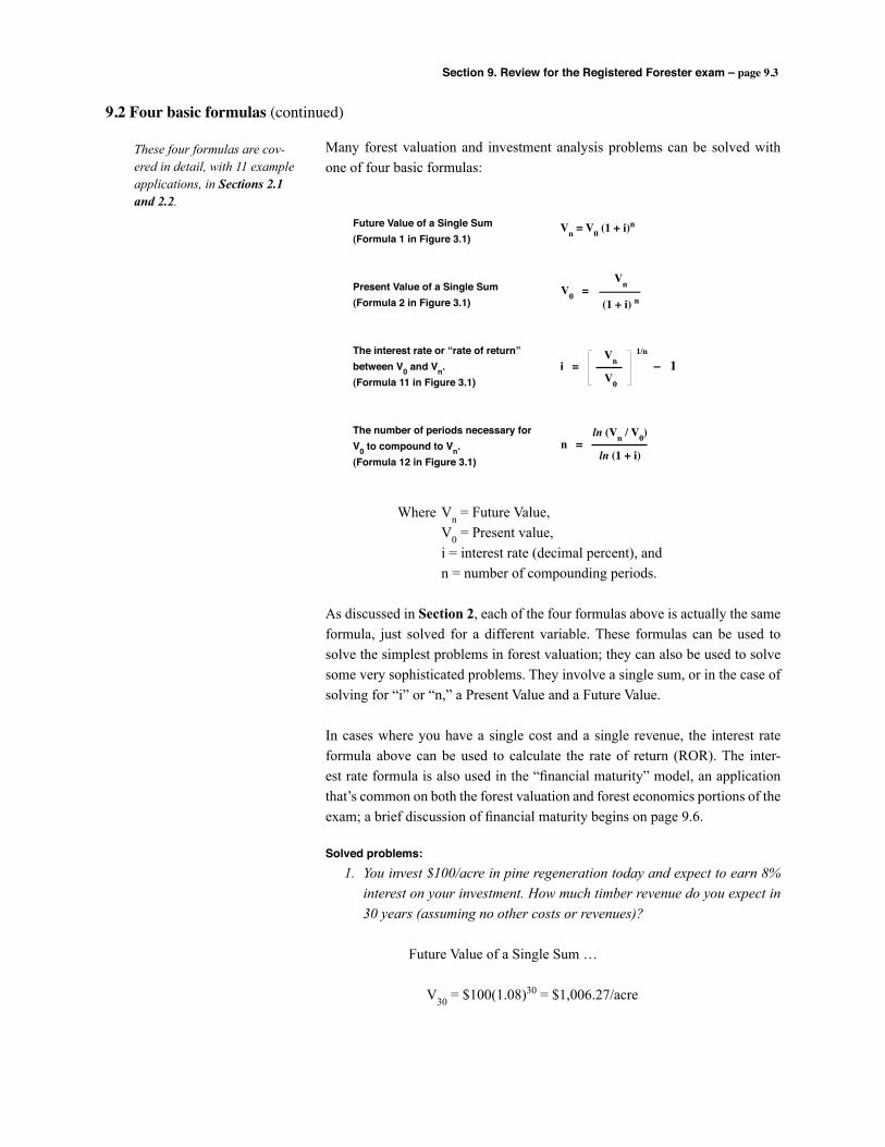
Section 9. Review for the Registered Forester exam – page 9.3
Many forest valuation and investment analysis problems can be solved with one of four basic formulas:
Where Vn = Future Value, V0 = Present value, i = interest rate (decimal percent), and n = number of compounding periods.
As discussed in Section 2, each of the four formulas above is actually the same formula, just solved for a different variable. These formulas can be used to solve the simplest problems in forest valuation; they can also be used to solve some very sophisticated problems. They involve a single sum, or in the case of solving for “i” or “n,” a Present Value and a Future Value.
In cases where you have a single cost and a single revenue, the interest rate formula above can be used to calculate the rate of return (ROR). The inter-est rate formula is also used in the “financial maturity” model, an application that’s common on both the forest valuation and forest economics portions of the exam; a brief discussion of financial maturity begins on page 9.6.
Solved problems: 1. You invest $100/acre in pine regeneration today and expect to earn 8%
interest on your investment. How much timber revenue do you expect in 30 years (assuming no other costs or revenues)?
Future Value of a Single Sum …
V30 = $100(1.08)30 = $1,006.27/acre
9.2 Four basic formulas (continued)
These four formulas are cov-ered in detail, with 11 example applications, in Sections 2.1 and 2.2.
Future Value of a Single Sum(Formula 1 in Figure 3.1)
Present Value of a Single Sum(Formula 2 in Figure 3.1)
The interest rate or “rate of return”between V0 and Vn.(Formula 11 in Figure 3.1)
The number of periods necessary forV0 to compound to Vn.(Formula 12 in Figure 3.1)
Vn = V0 (1 + i)n
V0 = Vn
(1 + i) n
i = – 1 Vn
V0
1/n
n = ln (Vn / V0)
ln (1 + i)
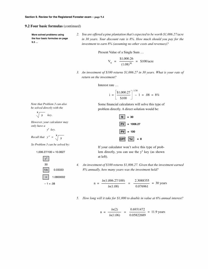
Section 9. Review for the Registered Forester exam – page 9.4
=
2. You are offered a pine plantation that’s expected to be worth $1,006.27/acre in 30 years. Your discount rate is 8%. How much should you pay for the investment to earn 8% (assuming no other costs and revenues)?
3. An investment of $100 returns $1,006.27 in 30 years. What is your rate of return on the investment?
9.2 Four basic formulas (continued)
More solved problems using the four basic formulas on page 9.3 …
Present Value of a Single Sum …
$1,000.26
(1.08)30V0 = = $100/acre
Interest rate …
$1,000.27
$100
1/30
i = – 1 = .08 = 8%
Some financial calculators will solve this type of problem directly. A direct solution would be:
If your calculator won’t solve this type of prob-lem directly, you can use the yx key (as shown at left).
N = 30
FV = 1006.27
PV = 100
CPT = 8%i
4. An investment of $100 returns $1,006.27. Given that the investment earned 8% annually, how many years was the investment held?
5. How long will it take for $1,000 to double in value at 6% annual interest?
n =ln(1,006.27/100)
ln(1.08)=
2.3088355
0.076961= 30 years
n =ln(2)
ln(1.06)=
0.6931472
0.05822689= 11.9 years
Note that Problem 3 can also be solved directly with the
yx
key.
However, your calculator may only have a yx key.
Recall that y-x =
So Problem 3 can be solved by:
1,006.27/100 = 10.0627
yx
yx
30
1/x 0.03333
1.0800002
– 1 = .08

Section 9. Review for the Registered Forester exam – page 9.5
i = – 1 = .075 = 7.5%
6a. You own a 10-year-old pine plantation that you expect to harvest at age 22. You’re considering a precommercial thinning operation. The thinning will cost $67/acre and will increase the final harvest value by $500 /acre. What is the ROR on the precommercial thinning investment?
This is a basic interest rate calculation. The Present Value is $67, the Future Value is $500, and n = 12 …
6b. You own a 10-year-old pine plantation that you expect to harvest at age 22. You’re considering a precommercial thinning operation. The thinning will cost $67/acre. You’re required to earn at least 10% on the investment. How much must harvest value increase to ensure a 10% compound annual rate of return?
This is a simple Future Value of a Single Sum problem …
V12 = $67 (1.10)12 = $210.27
6c. You own a 10-year-old pine plantation that you expect to harvest at age 22. You’re considering a precommercial thinning operation. The thinning will cost $67/acre. You’re required to earn at least 10% on the investment. If pulpwood is expected to be worth $23/cord in 12 years, how much must harvest increase to ensure a 10% compound annual rate of return?
This is the same problem as 6b, only in cords rather than dollars …
V12 = $67 (1.10)12 = $210.27
$210.27 ÷ $23 per cord = 9.14 cords
7. A timber stand is worth $100,000 today. In three years it’s expected to be worth $124,229.69. What annual rate of return would be earned by holding the stand for three more years?
9.2 Four basic formulas (continued)
More solved problems using the four basic formulas on page 9.3 …
$500.00
$67.00
1/12
i = – 1 = 18.23 = 18.23%
$124,229.69
$100,000.00
1/3
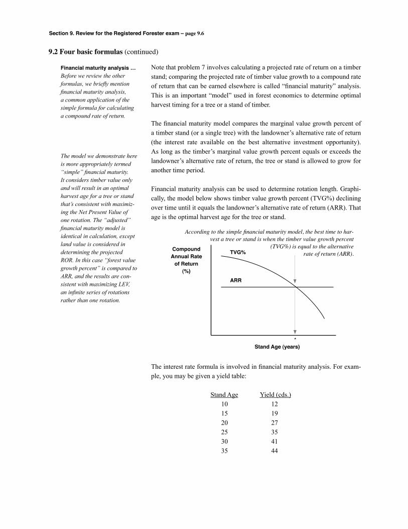
Section 9. Review for the Registered Forester exam – page 9.6
Note that problem 7 involves calculating a projected rate of return on a timber stand; comparing the projected rate of timber value growth to a compound rate of return that can be earned elsewhere is called “financial maturity” analysis. This is an important “model” used in forest economics to determine optimal harvest timing for a tree or a stand of timber.
The financial maturity model compares the marginal value growth percent of a timber stand (or a single tree) with the landowner’s alternative rate of return (the interest rate available on the best alternative investment opportunity). As long as the timber’s marginal value growth percent equals or exceeds the landowner’s alternative rate of return, the tree or stand is allowed to grow for another time period.
Financial maturity analysis can be used to determine rotation length. Graphi-cally, the model below shows timber value growth percent (TVG%) declining over time until it equals the landowner’s alternative rate of return (ARR). That age is the optimal harvest age for the tree or stand.
The interest rate formula is involved in financial maturity analysis. For exam-ple, you may be given a yield table:
Stand Age Yield (cds.) 10 12 15 19 20 27 25 35 30 41 35 44
9.2 Four basic formulas (continued)
Financial maturity analysis …Before we review the other formulas, we briefly mention financial maturity analysis, a common application of the simple formula for calculating a compound rate of return.
The model we demonstrate here is more appropriately termed “simple” financial maturity. It considers timber value only and will result in an optimal harvest age for a tree or stand that’s consistent with maximiz-ing the Net Present Value of one rotation. The “adjusted” financial maturity model is identical in calculation, except land value is considered in determining the projected ROR. In this case “forest value growth percent” is compared to ARR, and the results are con-sistent with maximizing LEV, an infinite series of rotations rather than one rotation.
TVG%
ARR
CompoundAnnual Rate
of Return(%)
Stand Age (years)
According to the simple financial maturity model, the best time to har-vest a tree or stand is when the timber value growth percent
(TVG%) is equal to the alternativerate of return (ARR).
*
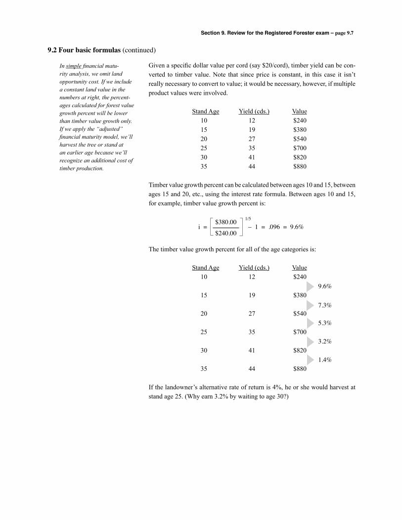
Section 9. Review for the Registered Forester exam – page 9.7
Given a specific dollar value per cord (say $20/cord), timber yield can be con-verted to timber value. Note that since price is constant, in this case it isn’t really necessary to convert to value; it would be necessary, however, if multiple product values were involved.
Stand Age Yield (cds.) Value 10 12 $240 15 19 $380 20 27 $540 25 35 $700 30 41 $820 35 44 $880
Timber value growth percent can be calculated between ages 10 and 15, between ages 15 and 20, etc., using the interest rate formula. Between ages 10 and 15, for example, timber value growth percent is:
The timber value growth percent for all of the age categories is:
Stand Age Yield (cds.) Value 10 12 $240
15 19 $380
20 27 $540
25 35 $700
30 41 $820
35 44 $880
If the landowner’s alternative rate of return is 4%, he or she would harvest at stand age 25. (Why earn 3.2% by waiting to age 30?)
9.2 Four basic formulas (continued)
In simple financial matu-rity analysis, we omit land opportunity cost. If we include a constant land value in the numbers at right, the percent-ages calculated for forest value growth percent will be lower than timber value growth only. If we apply the “adjusted” financial maturity model, we’ll harvest the tree or stand at an earlier age because we’ll recognize an additional cost of timber production.
$380.00
$240.00
1/5
i = – 1 = .096 = 9.6%
9.6%
7.3%
5.3%
3.2%
1.4%
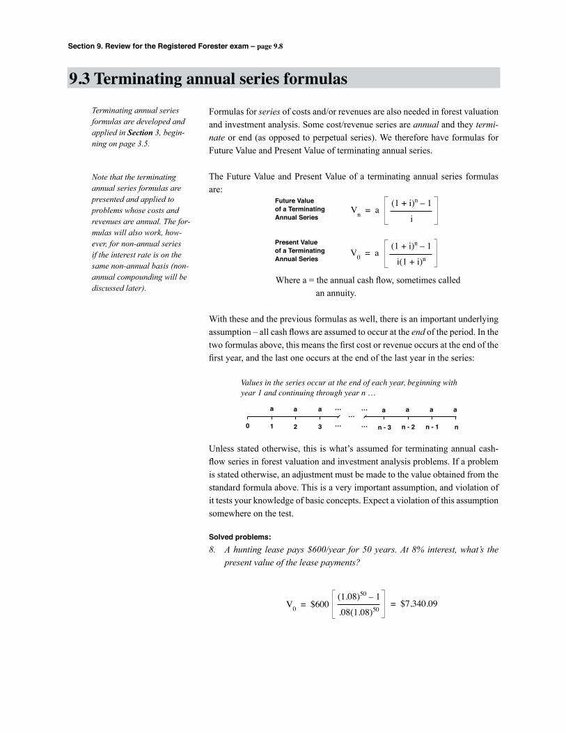
Section 9. Review for the Registered Forester exam – page 9.8
Formulas for series of costs and/or revenues are also needed in forest valuation and investment analysis. Some cost/revenue series are annual and they termi-nate or end (as opposed to perpetual series). We therefore have formulas for Future Value and Present Value of terminating annual series.
The Future Value and Present Value of a terminating annual series formulas are:
Where a = the annual cash flow, sometimes called an annuity.
With these and the previous formulas as well, there is an important underlying assumption – all cash flows are assumed to occur at the end of the period. In the two formulas above, this means the first cost or revenue occurs at the end of the first year, and the last one occurs at the end of the last year in the series:
Unless stated otherwise, this is what’s assumed for terminating annual cash-flow series in forest valuation and investment analysis problems. If a problem is stated otherwise, an adjustment must be made to the value obtained from the standard formula above. This is a very important assumption, and violation of it tests your knowledge of basic concepts. Expect a violation of this assumption somewhere on the test.
Solved problems:8. A hunting lease pays $600/year for 50 years. At 8% interest, what’s the
present value of the lease payments?
9.3 Terminating annual series formulas
Terminating annual series formulas are developed and applied in Section 3, begin-ning on page 3.5.
Note that the terminating annual series formulas are presented and applied to problems whose costs and revenues are annual. The for-mulas will also work, how-ever, for non-annual series if the interest rate is on the same non-annual basis (non-annual compounding will be discussed later).
(1 + i)n – 1
iVn = a
Future Valueof a TerminatingAnnual Series
Present Valueof a TerminatingAnnual Series
(1 + i)n – 1
i(1 + i)nV0 = a
0 1 2 3 ……
…
……
nn - 2 n - 1n - 3
a a a a a aa
Values in the series occur at the end of each year, beginning with year 1 and continuing through year n …
(1.08)50 – 1
.08(1.08)50V0 = $600 = $7,340.09
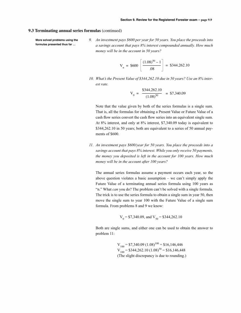
Section 9. Review for the Registered Forester exam – page 9.9
9. An investment pays $600 per year for 50 years. You place the proceeds into a savings account that pays 8% interest compounded annually. How much money will be in the account in 50 years?
10. What’s the Present Value of $344,262.10 due in 50 years? Use an 8% inter-est rate.
Note that the value given by both of the series formulas is a single sum. That is, all the formulas for obtaining a Present Value or Future Value of a cash flow series convert the cash flow series into an equivalent single sum. At 8% interest, and only at 8% interest, $7,340.09 today is equivalent to $344,262.10 in 50 years; both are equivalent to a series of 50 annual pay-ments of $600.
11. An investment pays $600/year for 50 years. You place the proceeds into a savings account that pays 8% interest. While you only receive 50 payments, the money you deposited is left in the account for 100 years. How much money will be in the account after 100 years?
The annual series formulas assume a payment occurs each year, so the
above question violates a basic assumption – we can’t simply apply the Future Value of a terminating annual series formula using 100 years as “n.” What can you do? The problem can’t be solved with a single formula. The trick is to use the series formula to obtain a single sum in year 50, then move the single sum to year 100 with the Future Value of a single sum formula. From problems 8 and 9 we know:
V0 = $7,340.09, and V50 = $344,262.10
Both are single sums, and either one can be used to obtain the answer to problem 11:
V100 = $7,340.09 (1.08)100 = $16,146,446 V100 = $344,262.10 (1.08)50 = $16,146,448 (The slight discrepancy is due to rounding.)
9.3 Terminating annual series formulas (continued)
More solved problems using the formulas presented thus far …
(1.08)50 – 1
.08Vn = $600 = $344,262.10
$344,262.10
(1.08)50V0 = = $7,340.09
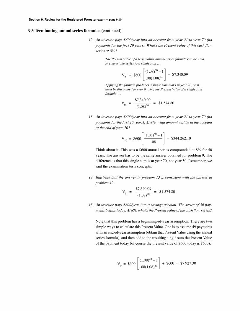
Section 9. Review for the Registered Forester exam – page 9.10
12. An investor pays $600/year into an account from year 21 to year 70 (no payments for the first 20 years). What’s the Present Value of this cash flow series at 8%?
13. An investor pays $600/year into an account from year 21 to year 70 (no payments for the first 20 years). At 8%, what amount will be in the account at the end of year 70?
Think about it. This was a $600 annual series compounded at 8% for 50 years. The answer has to be the same answer obtained for problem 9. The difference is that this single sum is at year 70, not year 50. Remember, we said the examination tests concepts.
14. Illustrate that the answer in problem 13 is consistent with the answer in problem 12.
15. An investor pays $600/year into a savings account. The series of 50 pay-ments begins today. At 8%, what’s the Present Value of the cash flow series?
Note that this problem has a beginning-of-year assumption. There are two simple ways to calculate this Present Value. One is to assume 49 payments with an end-of-year assumption (obtain that Present Value using the annual series formula), and then add to the resulting single sum the Present Value of the payment today (of course the present value of $600 today is $600):
9.3 Terminating annual series formulas (continued)
The Present Value of a terminating annual series formula can be used to convert the series to a single sum …
Applying the formula produces a single sum that’s in year 20, so it must be discounted to year 0 using the Present Value of a single sum formula …
(1.08)50 – 1
.08(1.08)50V20 = $600 = $7,340.09
$7,340.09
(1.08)20V0 = = $1,574.80
(1.08)50 – 1
.08V70 = $600 = $344,262.10
$7,340.09
(1.08)70V0 = = $1,574.80
(1.08)49 – 1
.08(1.08)49V0 = $600 + $600 = $7,927.30
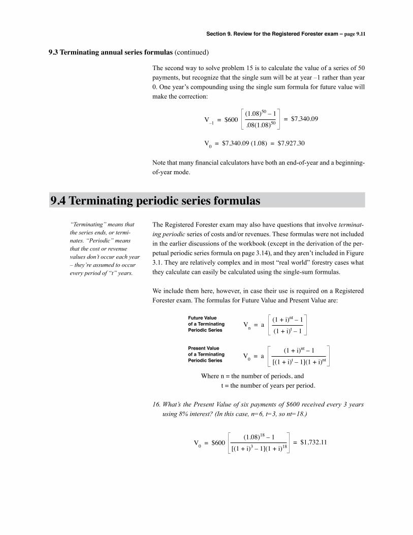
Section 9. Review for the Registered Forester exam – page 9.11
The second way to solve problem 15 is to calculate the value of a series of 50 payments, but recognize that the single sum will be at year –1 rather than year 0. One year’s compounding using the single sum formula for future value will make the correction:
Note that many financial calculators have both an end-of-year and a beginning-of-year mode.
9.3 Terminating annual series formulas (continued)
(1.08)50 – 1
.08(1.08)50V–1 = $600 = $7,340.09
V0 = $7,340.09 (1.08) = $7,927.30
The Registered Forester exam may also have questions that involve terminat-ing periodic series of costs and/or revenues. These formulas were not included in the earlier discussions of the workbook (except in the derivation of the per-petual periodic series formula on page 3.14), and they aren’t included in Figure 3.1. They are relatively complex and in most “real world” forestry cases what they calculate can easily be calculated using the single-sum formulas.
We include them here, however, in case their use is required on a Registered Forester exam. The formulas for Future Value and Present Value are:
Where n = the number of periods, and t = the number of years per period.
16. What’s the Present Value of six payments of $600 received every 3 years using 8% interest? (In this case, n=6, t=3, so nt=18.)
9.4 Terminating periodic series formulas
“Terminating” means that the series ends, or termi-nates. “Periodic” means that the cost or revenue values don’t occur each year – they’re assumed to occur every period of “t” years.
(1 + i)nt – 1
(1 + i)t – 1Vn = a
Future Valueof a TerminatingPeriodic Series
Present Valueof a TerminatingPeriodic Series
(1 + i)nt – 1
[(1 + i)t – 1](1 + i)ntV0 = a
(1.08)18 – 1
[(1 + i)3 – 1](1 + i)18V0 = $600 = $1,732.11

Section 9. Review for the Registered Forester exam – page 9.12
Note that problem 16 can also be worked by discounting each of the six payments with the single sum formula
Year Payment Present Value 3 $600 $476.30 6 $600 $378.10 9 $600 $300.15 12 $600 $238.27 15 $600 $189.15 18 $600 $150.15
Present value of the series = $1,732.12
17. What’s the Future Value of six payments of $600 that are made at three-year intervals?
You could also solve problem 17 with the result from problem 16 and the single sum formula for Future Value:
V18 = $1,732.12 (1.08)18 = $6,921.59
18. An investor pays $600 into a savings account in odd years and $1,200 into the account in even years. The cash flow diagram is:
How much money will be in this account after 50 years at 8% interest?
There are two “simple” ways to solve this problem. The first is to view the series as a terminating annual series of $600 per year and a terminating periodic series of an additional $600 every other year.
9.4 Terminating periodic series formulas (continued)
(1.08)18 – 1
(1.08)3 – 1V18 = $600 = $6,921.56
…0 1 2 3 4 47 48 49 50
$600 $600 $600 $600 $1,200 $1,200 $1,200 $1,200
V50 = $600(1.08)50 – 1
.08= $344,262.10
V50 = $600(1.08)50 – 1
(1.08)2 – 1= $165,510.63
Total =$509,772.73
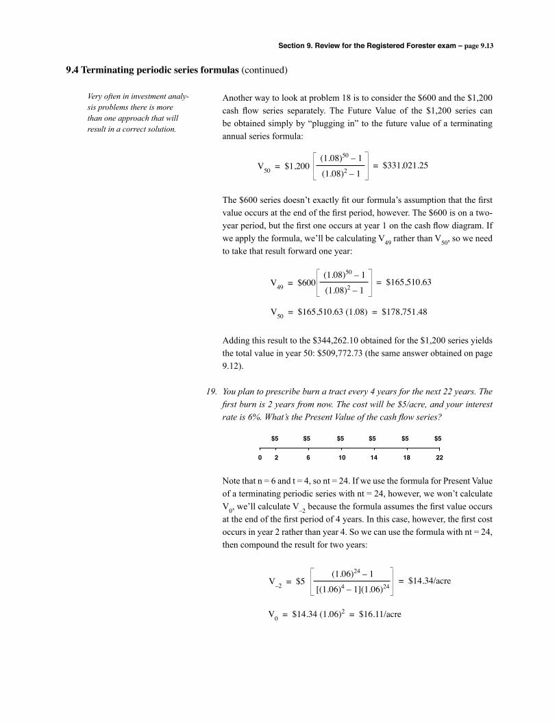
Section 9. Review for the Registered Forester exam – page 9.13
Another way to look at problem 18 is to consider the $600 and the $1,200 cash flow series separately. The Future Value of the $1,200 series can be obtained simply by “plugging in” to the future value of a terminating annual series formula:
The $600 series doesn’t exactly fit our formula’s assumption that the first value occurs at the end of the first period, however. The $600 is on a two-year period, but the first one occurs at year 1 on the cash flow diagram. If we apply the formula, we’ll be calculating V49 rather than V50, so we need to take that result forward one year:
Adding this result to the $344,262.10 obtained for the $1,200 series yields the total value in year 50: $509,772.73 (the same answer obtained on page 9.12).
19. You plan to prescribe burn a tract every 4 years for the next 22 years. The first burn is 2 years from now. The cost will be $5/acre, and your interest rate is 6%. What’s the Present Value of the cash flow series?
Note that n = 6 and t = 4, so nt = 24. If we use the formula for Present Value of a terminating periodic series with nt = 24, however, we won’t calculate V0, we’ll calculate V–2 because the formula assumes the first value occurs at the end of the first period of 4 years. In this case, however, the first cost occurs in year 2 rather than year 4. So we can use the formula with nt = 24, then compound the result for two years:
9.4 Terminating periodic series formulas (continued)
Very often in investment analy-sis problems there is more than one approach that will result in a correct solution.
V50 = $1,200(1.08)50 – 1
(1.08)2 – 1= $331,021.25
V49 = $600(1.08)50 – 1
(1.08)2 – 1= $165,510.63
V50 = $165,510.63 (1.08) = $178,751.48
0 2 6 10 14 18 22
$5 $5 $5 $5 $5 $5
(1.06)24 – 1
[(1.06)4 – 1](1.06)24V–2 = $5 = $14.34/acre
V0 = $14.34 (1.06)2 = $16.11/acre
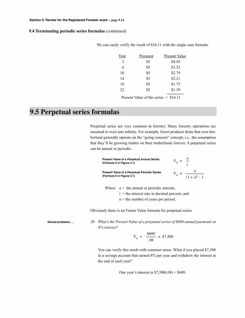
Section 9. Review for the Registered Forester exam – page 9.14
We can easily verify the result of $16.11 with the single sum formula:
Year Payment Present Value 2 $5 $4.45 6 $5 $3.52 10 $5 $2.79 14 $5 $2.21 18 $5 $1.75 22 $5 $1.39
Present Value of the series = $16.11
9.4 Terminating periodic series formulas (continued)
Perpetual series are very common in forestry. Many forestry operations are assumed to exist into infinity. For example, forest products firms that own tim-berland generally operate on the “going concern” concept, i.e., the assumption that they’ll be growing timber on their timberlands forever. A perpetual series can be annual or periodic:
Where a = the annual or periodic amount, i = the interest rate in decimal percent, and n = the number of years per period.
Obviously there is no Future Value formula for perpetual series.
20. What’s the Present Value of a perpetual series of $600 annual payments at 8% interest?
You can verify this result with common sense. What if you placed $7,500 in a savings account that earned 8% per year and withdrew the interest at the end of each year?
One year’s interest is $7,500(.08) = $600.
9.5 Perpetual series formulas
Present Value of a Perpetual Periodic Series(Formula 6 in Figure 3.1)
Present Value of a Perpetual Annual Series(Formula 5 in Figure 3.1)
ai
V0 =
a(1 + i)n – 1
V0 =
Solved problems …
$600.08
V0 = = $7,500
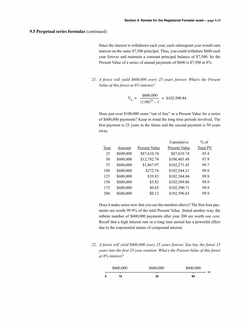
Section 9. Review for the Registered Forester exam – page 9.15
9.5 Perpetual series formulas (continued)
Since the interest is withdrawn each year, each subsequent year would earn interest on the same $7,500 principal. Thus, you could withdraw $600 each year forever and maintain a constant principal balance of $7,500. So the Present Value of a series of annual payments of $600 is $7,500 at 8%.
21. A forest will yield $600,000 every 25 years forever. What’s the Present Value of this forest at 8% interest?
Does just over $100,000 seem “out of line” as a Present Value for a series of $600,000 payments? Keep in mind the long time periods involved. The first payment is 25 years in the future and the second payment is 50 years away.
Cumulative % of Year Amount Present Value Present Value Total PV 25 $600,000 $87,610.74 $87,610.74 85.4 50 $600,000 $12,792.74 $100,403.48 97.9 75 $600,000 $1,867.97 $102,271.45 99.7 100 $600,000 $272.76 $102,544.21 99.9 125 $600,000 $39.83 $102,584.04 99.9 150 $600,000 $5.82 $102,589.86 99.9 175 $600,000 $0.85 $102,590.71 99.9 200 $600,000 $0.12 $102,590.83 99.9
Does it make sense now that you see the numbers above? The first four pay-ments are worth 99.9% of the total Present Value. Stated another way, the infinite number of $600,000 payments after year 200 are worth one cent. Recall that a high interest rate or a long time period has a powerful effect due to the exponential nature of compound interest.
22. A forest will yield $600,000 every 25 years forever. You buy the forest 15 years into the first 25-year rotation. What’s the Present Value of this forest at 8% interest?
$600,000(1.08)25 – 1
V0 = = $102,590.84
0 10 35 60
$600,000 $600,000 $600,000
8
Section 9. Review for the Registered Forester exam – page 9.16
9.5 Perpetual series formulas (continued)
23. What’s the Present Value of a perpetual annual series that pays $6,000 every odd year and $12,000 every even year? Use 8% interest.
Like problem 18, we present two solutions.
Solution 1 … Solve for the Present Value of a perpetual annual series of $6,000 every
year. Add to that the Present Value of a perpetual periodic series of $6,000 every two years:
Solution 2 … Solve for the Present Value of each series directly. The $12,000 series is
every two years starting in year two, so it meets the end-of-period assump-tion. The $6,000 series is every two years starting in year one, so it violates the end-of-period assumption – it’s “off kilter” by one year. One year of compounding will make the correct adjustment:
Solved problems …$600,000
(1.08)25 – 1V–15 = = $102,590.84
V0 = $102,590.84 (1.08)15 = $325,435.50
$6,000.08
V0 = = $75,000.00
$6,000(1.08)2 – 1
V0 = = $36,057.69
Total = $111,057.69
$12,000(1.08)2 – 1
V0 = = $72,115.39
Total V0 = $72,115.39 + $38,942.31 = $111,057.69
$6,000(1.08)2 – 1
V–1 = = $36,057.69 …
V0 = $36,057.69 (1.08) = $38,942.31
Must be compounded for one year to obtain V0 for the $6,000 series
Section 9. Review for the Registered Forester exam – page 9.17
9.5 Perpetual series formulas (continued)
24. What’s the Present Value of a perpetual series of $6,000 received in 20 years, and every 30 years thereafter? (Use 8% interest.)
25. What’s the Present Value of a perpetual series of $6,000 received today and every 30 years thereafter? (Use 8% interest.)
This is a standard perpetual periodic series except for the payment today. Add the present value of a $6,000 payment today to the value of the stan-dard series:
$6,000(1.08)30 – 1
V–10 = = $662.06
V0 = $662.064 (1.08)10 = $1,429.33
$6,000(1.08)30 – 1
V0 = + $6,000 = $6,662.06
These are the last two standard formulas. The installment payment formula calculates the payment over a specific period of time that’s necessary to repay a specific amount borrowed. An example would be the payment over 48 months that equates to a $30,000 pickup truck. The installment payment formula is also called the capital recovery formula.
The sinking fund formula, meanwhile, calculates the payment that’s equivalent to a specific future value. An example would be the annual payments necessary to accumulate $100,000 at the end of 20 years.
9.6 Installment payments and sinking funds
The installment payment formula(Formula 9 in Figure 3.1)
The “sinking fund” formula(Formula 7 in Figure 3.1) Pann. = Vn
i(1 + i)n – 1
Pann. = V0i(1 + i)n
(1 + i)n – 1
Where Pann. = the annual payment.
Section 9. Review for the Registered Forester exam – page 9.18
9.6 Installment payments and sinking funds (continued)
26. You need $1,000,000 to replace logging equipment in six years. How much money would you need to deposit into an account paying 8% interest each year to accumulate the necessary amount?
27. You borrow $30,000 at 8% interest to purchase a new truck. What’s your monthly payment if you have 48 payments?
Note that your monthly interest rate will be .08 ÷ 12 = 0.0067 = .67%. (Non-annual compounding is covered in the next subsection; for now, simply calculate installment payments for n = 48 and i = 0.67%.)
Solved problems …
Pann. = $1,000,000.08
(1.08)6 – 1= $136,315.39
Pann. = $30,0000.0067(1.0067)48
(1.0067)48 – 1= $732.95
The Registered Forester examination may include a problem or two with non-annual compounding (like problem 27 above). By non-annual compounding, we mean semi-annual, quarterly, monthly, or daily compounding. All of the formulas presented earlier can be used for non-annual compounding. Only two adjustments are necessary:
• Let m = the number of compounding periods in a year. If n = the number of years, n*m = the total number of compounding periods.
• Instead of i = annual interest rate, use i = annual rate ÷ m. This will be the monthly interest rate, the quarterly rate, etc., depending on how many compounding periods are in a year.
28. You place $1,000 into an account paying 8% compounded quarterly. How much will be in the account after six years?
m = number of compounding periods per year = 4, and n = 6, so n*m = 24 i = .08 ÷ 4 = 0.02 = 2% per quarter
V6 = $1,000 (1.02)24 = $1,608.44
9.7 Non-annual compounding periods
Solved problems …
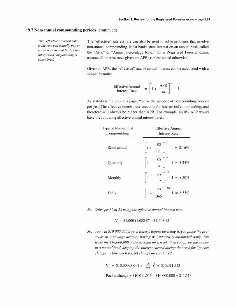
Section 9. Review for the Registered Forester exam – page 9.19
9.7 Non-annual compounding periods (continued)
The “effective” interest rate can also be used to solve problems that involve non-annual compounding. Most banks state interest on an annual basis called the “APR” or “Annual Percentage Rate.” On a Registered Forester exam, assume all interest rates given are APRs (unless stated otherwise).
Given an APR, the “effective” rate of annual interest can be calculated with a simple formula:
As stated on the previous page, “m” is the number of compounding periods per year.The effective interest rate accounts for interperiod compounding, and therefore will always be higher than APR. For example, an 8% APR would have the following effective annual interest rates:
29. Solve problem 28 using the effective annual interest rate.
V6 = $1,000 (1.0824)6 = $1,608.15
30. You win $10,000,000 from a lottery. Before investing it, you place the pro-ceeds in a savings account paying 6% interest compounded daily. You leave the $10,000,000 in the account for a week, then you invest the money in a mutual fund, keeping the interest earned during the week for “pocket change.” How much pocket change do you have?
The “effective” interest rate is the rate you actually pay or earn on an annual basis when interperiod compounding is considered.
Effective AnnualInterest Rate =
APR
m1 +
m
– 1
.08
21 +
2
– 1 = 8.16%
.08
41 +
4
– 1 = 8.24%
.08
121 +
12
– 1 = 8.30%
.08
3651 +
365
– 1 = 8.33%
Effective AnnualInterest Rate
Type of Non-annualCompounding
Semi-annual
Quarterly
Monthly
Daily
Vn = $10,000,000 (1 + )7 = $10,011,513
Pocket change = $10,011,513 – $10,000,000 = $11,513
.06365
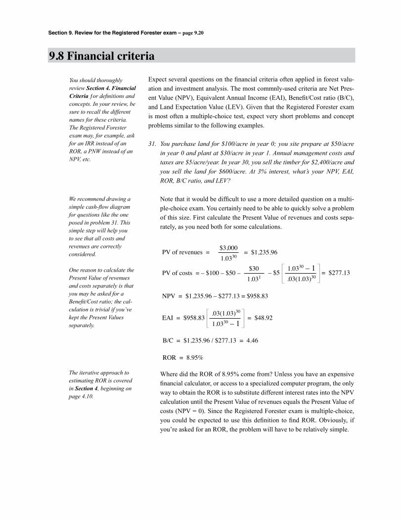
Section 9. Review for the Registered Forester exam – page 9.20
Expect several questions on the financial criteria often applied in forest valu-ation and investment analysis. The most commnly-used criteria are Net Pres-ent Value (NPV), Equivalent Annual Income (EAI), Benefit/Cost ratio (B/C), and Land Expectation Value (LEV). Given that the Registered Forester exam is most often a multiple-choice test, expect very short problems and concept problems similar to the following examples.
31. You purchase land for $100/acre in year 0; you site prepare at $50/acre in year 0 and plant at $30/acre in year 1. Annual management costs and taxes are $5/acre/year. In year 30, you sell the timber for $2,400/acre and you sell the land for $600/acre. At 3% interest, what’s your NPV, EAI, ROR, B/C ratio, and LEV?
Note that it would be difficult to use a more detailed question on a multi-ple-choice exam. You certainly need to be able to quickly solve a problem of this size. First calculate the Present Value of revenues and costs sepa-rately, as you need both for some calculations.
Where did the ROR of 8.95% come from? Unless you have an expensive financial calculator, or access to a specialized computer program, the only way to obtain the ROR is to substitute different interest rates into the NPV calculation until the Present Value of revenues equals the Present Value of costs (NPV = 0). Since the Registered Forester exam is multiple-choice, you could be expected to use this definition to find ROR. Obviously, if you’re asked for an ROR, the problem will have to be relatively simple.
9.8 Financial criteria
PV of revenues = $3,0001.0330
= $1,235.96
PV of costs = – $100 – $50 –$30
1.031= $277.13– $5 1.0330 – 1
.03(1.03)30
NPV = $1,235.96 – $277.13 = $958.83
EAI = $958.83 = $48.92.03(1.03)30
1.0330 – 1
B/C = $1,235.96 / $277.13 = 4.46
ROR = 8.95%
You should thoroughly review Section 4. Financial Criteria ƒor definitions and concepts. In your review, be sure to recall the different names for these criteria. The Registered Forester exam may, for example, ask for an IRR instead of an ROR, a PNW instead of an NPV, etc.
We recommend drawing a simple cash-flow diagram for questions like the one posed in problem 31. This simple step will help you to see that all costs and revenues are correctly considered.
One reason to calculate the Present Value of revenues and costs separately is that you may be asked for a Benefit/Cost ratio; the cal-culation is trivial if you’ve kept the Present Values separately.
The iterative approach to estimating ROR is covered in Section 4, beginning on page 4.10.

Section 9. Review for the Registered Forester exam – page 9.21
9.8 Financial criteria (continued)
For example, suppose we asked you for the NPV in problem 31, then in prob-lem 32 asked you for the ROR to the nearest whole percent. Assume your mul-tiple-choice answers are: a. 2% b. 3% c. 5% d. 9%
If NPV is positive, the ROR is higher than the interest rate you used to calculate NPV (see Figure 4.4 on page 4.11). Using a higher interest rate means you’ll obtain a lower value for NPV, and the ROR is the interest rate where NPV = 0. Since NPV = $958.83 using 3% interest, answers “a” and “b” above must be incorrect.
Given the magnitude of the NPV, one might guess that 9% is correct. Only one calculation is necessary to see if 5% or 9% is the ROR. If you try 5% and recalculate NPV, it will still be positive, and you’ll know that 9% has to be the correct answer. If you use 9% and recalculate NPV, you obtain:
The EAI formula was used in problem 31 (as shown in Figure 4.2 on page 4.4). It’s the same formula used to calculate installment payments, so it’s included in most financial calculators.
How would you calculate LEV for problem 31? We can calculate LEV by making use of the previously calculated NPV. LEV requires the Future Value of one rotation for the numerator. The NPV can be used to obtain this Future Value, but the LEV calculation doesn’t include land cost; land value is what you’re calculating so it can’t be included in the future value of the first rotation.
Note that the NPV calculations in problem 31 included land cost. If land cost is subtracted from NPV, the NPV without land cost can be directly compounded to obtain the Future Value of a single rotation. This Future Value can then be used to calculate LEV.
NPV is very close to zero at 9%, so the ROR estimate would be 9%.
NPV =$3,0001.0930
– $100 – $50 – $301.091
1.0930 – 1.09(1.09)30
– $5
= – $2.77
$811.64(1.03)30
(1.03)30 – 1
NPV without land = $958.83 + $100 – $6001.0330
= $811.64
LEV = = $1,380.31
In Section 4, the LEV discus-sion begins on page 4.18.
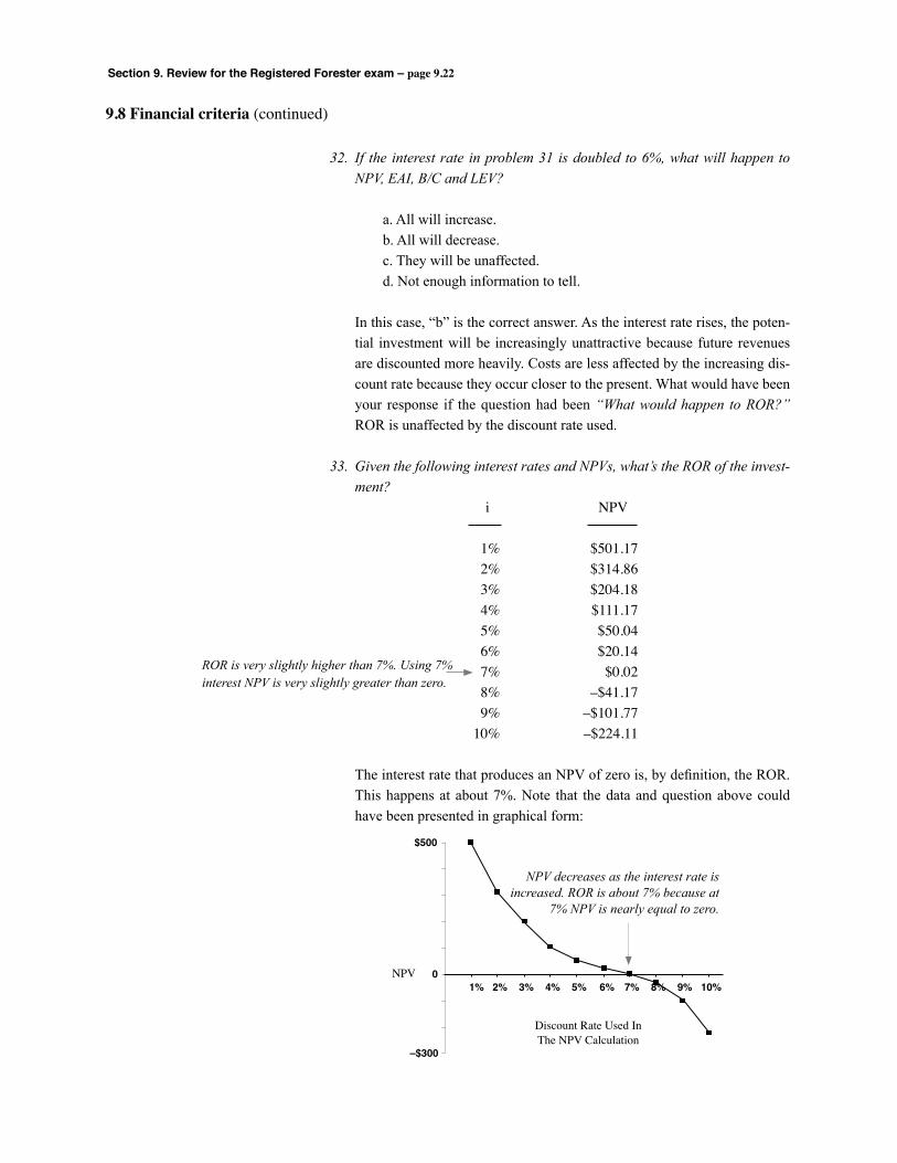
Section 9. Review for the Registered Forester exam – page 9.22
9.8 Financial criteria (continued)
32. If the interest rate in problem 31 is doubled to 6%, what will happen to NPV, EAI, B/C and LEV?
a. All will increase. b. All will decrease. c. They will be unaffected. d. Not enough information to tell.
In this case, “b” is the correct answer. As the interest rate rises, the poten-tial investment will be increasingly unattractive because future revenues are discounted more heavily. Costs are less affected by the increasing dis-count rate because they occur closer to the present. What would have been your response if the question had been “What would happen to ROR?” ROR is unaffected by the discount rate used.
33. Given the following interest rates and NPVs, what’s the ROR of the invest-ment?
i NPV 1% $501.17 2% $314.86 3% $204.18 4% $111.17 5% $50.04 6% $20.14 7% $0.02 8% –$41.17 9% –$101.77 10% –$224.11
The interest rate that produces an NPV of zero is, by definition, the ROR. This happens at about 7%. Note that the data and question above could have been presented in graphical form:
ROR is very slightly higher than 7%. Using 7% interest NPV is very slightly greater than zero.
$500
0
–$300
1% 2% 3% 4% 5% 6% 7% 8% 9% 10%NPV
Discount Rate Used InThe NPV Calculation
NPV decreases as the interest rate is increased. ROR is about 7% because at
7% NPV is nearly equal to zero.
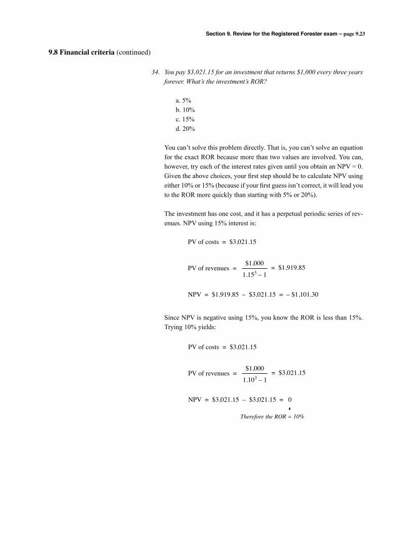
Section 9. Review for the Registered Forester exam – page 9.23
9.8 Financial criteria (continued)
34. You pay $3,021.15 for an investment that returns $1,000 every three years forever. What’s the investment’s ROR?
a. 5% b. 10% c. 15% d. 20%
You can’t solve this problem directly. That is, you can’t solve an equation for the exact ROR because more than two values are involved. You can, however, try each of the interest rates given until you obtain an NPV = 0. Given the above choices, your first step should be to calculate NPV using either 10% or 15% (because if your first guess isn’t correct, it will lead you to the ROR more quickly than starting with 5% or 20%).
The investment has one cost, and it has a perpetual periodic series of rev-enues. NPV using 15% interest is:
Since NPV is negative using 15%, you know the ROR is less than 15%. Trying 10% yields:
PV of costs = $3,021.15
PV of revenues =
NPV = $1,919.85 – $3,021.15 = – $1,101.30
$1,000
1.153 – 1= $1,919.85
PV of costs = $3,021.15
PV of revenues =
NPV = $3,021.15 – $3,021.15 = 0
$1,000
1.103 – 1= $3,021.15
Therefore the ROR = 10%
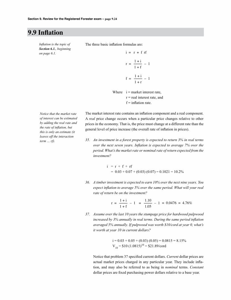
Section 9. Review for the Registered Forester exam – page 9.24
The three basic inflation formulas are:
Where i = market interest rate, r = real interest rate, and f = inflation rate.
The market interest rate contains an inflation component and a real component. A real price change occurs when a particular price changes relative to other prices in the economy. That is, the price must change at a different rate than the general level of price increase (the overall rate of inflation in prices).
35. An investment in a forest property is expected to return 3% in real terms over the next seven years. Inflation is expected to average 7% over the period. What’s the market rate or nominal rate of return expected from the investment?
i = r + f + rf = 0.03 + 0.07 + (0.03) (0.07) = 0.1021 = 10.2%
36. A timber investment is expected to earn 10% over the next nine years. You expect inflation to average 5% over the same period. What will your real rate of return be on the investment?
37. Assume over the last 10 years the stumpage price for hardwood pulpwood increased by 3% annually in real terms. During the same period inflation averaged 5% annually. If pulpwood was worth $10/cord at year 0, what’s it worth at year 10 in current dollars?
i = 0.03 + 0.05 + (0.03) (0.05) = 0.0815 = 8.15% V10 = $10 (1.0815)10 = $21.89/cord
Notice that problem 37 specified current dollars. Current dollar prices are actual market prices charged in any particular year. They include infla-tion, and may also be referred to as being in nominal terms. Constant dollar prices are fixed purchasing power dollars relative to a base year.
9.9 InflationInflation is the topic of Section 6.1., beginning on page 6.1. i = r + f rf
r = – 1
f = – 1
1 + i1 + f
1 + i1 + r
r = – 11 + i1 + f
= – 11.101.05
= 0.0476 = 4.76%
Notice that the market rate of interest can be estimated by adding the real rate and the rate of inflation, but this is only an estimate (it leaves off the interaction term … rf).

Section 9. Review for the Registered Forester exam – page 9.25
Taxes that relate to forest investments are a favorite Registered Forester exam topic. The mathematics are simple, but the concepts aren’t easy for many foresters. You’ll need to understand the basics of forest taxation. Specifically, know the definition of:
P ordinary income, P capital gains income, P capitalized, P expensed, P original cost basis, P adjusted basis, P land, timber, young growth, and plantation accounts, P depletion, P depletion rate, P depletion allowance, P fair market value, P tax deduction, P tax credit, P 7-year amortization, P after-tax investment analysis.
Income is assigned to one of two federal income tax categories: ordinary income and capital gains income. Ordinary income is the net profit that comes from the economic activity of a corporation or an individual. Capital gains (or losses) result when a capital asset is sold for more (or less) than its book value.
A capital asset is any asset that’s not normally bought or sold in the business of an individual or firm. Internal Revenue Service (IRS) regulations define which assets may be considered capital assets, including a minimum length of time an asset must be held for capital gains treatment. Capital gains income has a maxi-mum tax rate that for many individuals and firms is lower than their marginal tax rate on ordinary income.
9.10 Income taxesMethods for after-tax analysis are the subject of Section 6.2, beginning on page 6.10.
9.9 Inflation (continued)
38. What would be the answer to problem 37 if we wanted to know the pulp-wood price in constant (year 0) dollars at year 10?
V10 = $10 (1.03)10 = $13.44/cord
Capital gains income has a maximum tax rate that for many individuals and firms is lower than their mar-ginal tax rate on ordinary income.
Section 9. Review for the Registered Forester exam – page 9.26
9.10 Income taxes (continued)
For federal income tax purposes, expenditures of a forest owner are classified as capital expenditures or ordinary expenditures. That is, legitimate expenditures are either capitalized or expensed.
Expenditures that are expensed are deducted in full in the year they’re incurred. Generally, if the benefits resulting from an expenditure occur in the current tax year, the expenditure is expensed. Examples of expensed costs are:
• tools of a short life (usually one year or less); • salaries of hired labor, foresters, lawyers, and accountants; • travel expenses; and • property, yield, and state taxes.
Expenditures that are capitalized are deducted in three ways:
1. “Non-wasting” assets like land – costs are deducted when the asset is sold;
2. “Wasting” assets like equipment and structures – costs are deducted over the useful life of the asset through depreciation; and
3. Certain resource-based assets like timber and oil – costs are deducted as the asset is sold or used (depleted).
Since there are three ways to capitalize costs, three accounts are used to record capital expenditures in forestry:
1. Land account; 2. Equipment account; and 3. Timber (Depletion) Account.
Capitalization is the process of recording an expenditure in a capital account, instead of deducting the expenditure from ordinary income in the year incurred. The dollar value in any capital account represents the total investment for that capital asset. The purchase price of a capital asset (including related acqui-sition costs) is called the original cost basis of the asset. The original basis may increase as capital improvements are made, or decrease as allowances for depletion or depreciation are claimed. Once adjustments are made to the origi-nal basis, the basis is referred to as the adjusted basis. In general, just the term basis may be used.
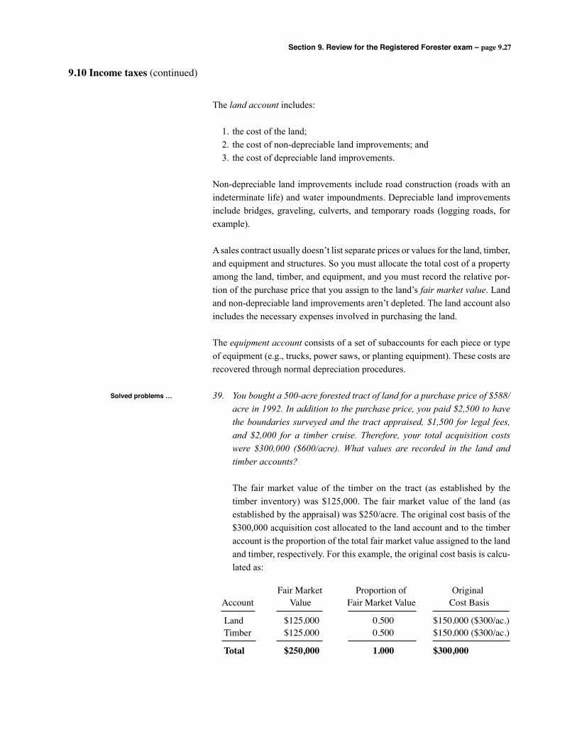
Section 9. Review for the Registered Forester exam – page 9.27
9.10 Income taxes (continued)
The land account includes:
1. the cost of the land; 2. the cost of non-depreciable land improvements; and 3. the cost of depreciable land improvements.
Non-depreciable land improvements include road construction (roads with an indeterminate life) and water impoundments. Depreciable land improvements include bridges, graveling, culverts, and temporary roads (logging roads, for example).
A sales contract usually doesn’t list separate prices or values for the land, timber, and equipment and structures. So you must allocate the total cost of a property among the land, timber, and equipment, and you must record the relative por-tion of the purchase price that you assign to the land’s fair market value. Land and non-depreciable land improvements aren’t depleted. The land account also includes the necessary expenses involved in purchasing the land.
The equipment account consists of a set of subaccounts for each piece or type of equipment (e.g., trucks, power saws, or planting equipment). These costs are recovered through normal depreciation procedures.
39. You bought a 500-acre forested tract of land for a purchase price of $588/acre in 1992. In addition to the purchase price, you paid $2,500 to have the boundaries surveyed and the tract appraised, $1,500 for legal fees, and $2,000 for a timber cruise. Therefore, your total acquisition costs were $300,000 ($600/acre). What values are recorded in the land and timber accounts?
The fair market value of the timber on the tract (as established by the timber inventory) was $125,000. The fair market value of the land (as established by the appraisal) was $250/acre. The original cost basis of the $300,000 acquisition cost allocated to the land account and to the timber account is the proportion of the total fair market value assigned to the land and timber, respectively. For this example, the original cost basis is calcu-lated as:
Solved problems …
Fair Market Proportion of OriginalAccount Value Fair Market Value Cost Basis
Land $125,000 0.500 $150,000 ($300/ac.) Timber $125,000 0.500 $150,000 ($300/ac.)
Total $250,000 1.000 $300,000
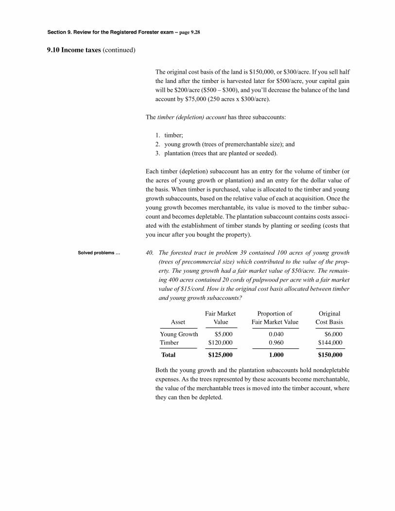
Section 9. Review for the Registered Forester exam – page 9.28
The original cost basis of the land is $150,000, or $300/acre. If you sell half the land after the timber is harvested later for $500/acre, your capital gain will be $200/acre ($500 – $300), and you’ll decrease the balance of the land account by $75,000 (250 acres x $300/acre).
The timber (depletion) account has three subaccounts:
1. timber; 2. young growth (trees of premerchantable size); and 3. plantation (trees that are planted or seeded).
Each timber (depletion) subaccount has an entry for the volume of timber (or the acres of young growth or plantation) and an entry for the dollar value of the basis. When timber is purchased, value is allocated to the timber and young growth subaccounts, based on the relative value of each at acquisition. Once the young growth becomes merchantable, its value is moved to the timber subac-count and becomes depletable. The plantation subaccount contains costs associ-ated with the establishment of timber stands by planting or seeding (costs that you incur after you bought the property).
40. The forested tract in problem 39 contained 100 acres of young growth (trees of precommercial size) which contributed to the value of the prop-erty. The young growth had a fair market value of $50/acre. The remain-ing 400 acres contained 20 cords of pulpwood per acre with a fair market value of $15/cord. How is the original cost basis allocated between timber and young growth subaccounts?
Both the young growth and the plantation subaccounts hold nondepletable expenses. As the trees represented by these accounts become merchantable, the value of the merchantable trees is moved into the timber account, where they can then be depleted.
9.10 Income taxes (continued)
Solved problems …
Fair Market Proportion of Original Asset Value Fair Market Value Cost Basis
Young Growth $5,000 0.040 $6,000Timber $120,000 0.960 $144,000
Total $125,000 1.000 $150,000
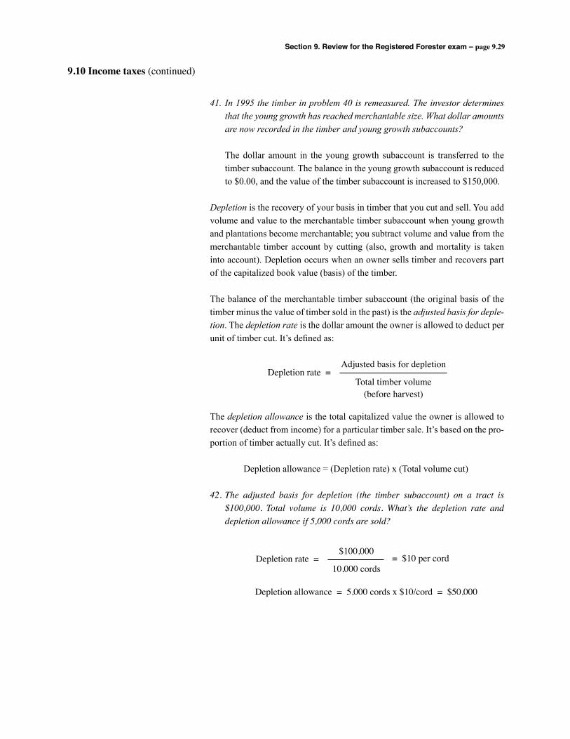
Section 9. Review for the Registered Forester exam – page 9.29
9.10 Income taxes (continued)
41. In 1995 the timber in problem 40 is remeasured. The investor determines that the young growth has reached merchantable size. What dollar amounts are now recorded in the timber and young growth subaccounts?
The dollar amount in the young growth subaccount is transferred to the timber subaccount. The balance in the young growth subaccount is reduced to $0.00, and the value of the timber subaccount is increased to $150,000.
Depletion is the recovery of your basis in timber that you cut and sell. You add volume and value to the merchantable timber subaccount when young growth and plantations become merchantable; you subtract volume and value from the merchantable timber account by cutting (also, growth and mortality is taken into account). Depletion occurs when an owner sells timber and recovers part of the capitalized book value (basis) of the timber.
The balance of the merchantable timber subaccount (the original basis of the timber minus the value of timber sold in the past) is the adjusted basis for deple-tion. The depletion rate is the dollar amount the owner is allowed to deduct per unit of timber cut. It’s defined as:
The depletion allowance is the total capitalized value the owner is allowed to recover (deduct from income) for a particular timber sale. It’s based on the pro-portion of timber actually cut. It’s defined as:
Depletion allowance = (Depletion rate) x (Total volume cut)
42. The adjusted basis for depletion (the timber subaccount) on a tract is $100,000. Total volume is 10,000 cords. What’s the depletion rate and depletion allowance if 5,000 cords are sold?
Depletion rate =Adjusted basis for depletion
Total timber volume(before harvest)
Depletion rate =$100,000
10,000 cords= $10 per cord
Depletion allowance = 5,000 cords x $10/cord = $50,000
Section 9. Review for the Registered Forester exam – page 9.30
9.10 Income taxes (continued)
An investment analysis should be on an after-tax basis since tax effects are a very real part of any transaction. Assume that the marginal tax rate for corpora-tions is 33% for ordinary income and 28% for capital gains. This is the tax rate that will affect marginal investments; thus, these tax rates are appropriate for after-tax investment analysis.
Where costs are expensed, the factor (1 – marginal tax rate) is used to convert a before-tax cost into an after-tax cost. For large corporations, for example, every additional dollar of ordinary income is worth ($1 – 33¢) = 67¢. Costs that can be expensed reduce taxes by 33¢ per dollar of expense, since the other 33¢ would have been paid in income taxes.
The same principles apply to private nonindustrial landowners, using their mar-ginal tax rates. An example is perhaps the best way to demonstrate these con-cepts.
43. A corporation asks you to determine the NPV of regenerating 40 acres. Site preparation and regeneration will cost $160/acre.* Property taxes and management costs will be $2.50/acre/year. Thinnings will occur at ages 16 and 22, and will yield five cords and eight cords/acre, respectively (20 percent of volume in both cases). Final harvest will occur at age 27 and will yield 66 cords/acre. Pulpwood is worth $19.50/cord. The corporation’s tax adjusted interest rate is 4%; its ordinary income is taxed at 46% and capital gains at 28%. What’s the investment’s NPV after taxes on a per acre basis?
After-tax investment analysis …
Solved problem …
*Note that for purposes of this example, the reforestation tax provisions of Public Law 96-451 are ignored. Seven-year amortization and the tax credit for reforestation are discussed later in this subsection.
Year
16
22
27
0
1-27
Item
Thinning
Final Harvest
Site Prep
0
Annual Costs
Before-tax
$97.50
$156.00
$1,287.00
$160.00
$2.50
After-tax
$79.16
$119.49
$955.31
$160.00
$1.35
Formula
11.0416
11.0422
11.0427
1.0427 – 1.04(1.04)27
Present Value
$42.26
$50.42
$331.31
$424.00
– $160.00
– $22.05
$182.05
Per acre present value of revenues =
Per acre present value of costs =
After-taxRevenues …
After-taxCosts …
Net Present Value after tax = $424.00 – $182.05 = $241.95
Here are the results of Problem 43 – followed by explanations of how the values were calculated …
Section 9. Review for the Registered Forester exam – page 9.31
Net Present Value after tax = $424.00 – $182.05 = $241.95
9.10 Income taxes (continued)
All of the revenue in problem 43 is treated as a capital gain. The capital gain calculation must account for the depletion allowance before the after-tax cash flow is determined.
At year 16 the after-tax cash flow was calculated on a per acre basis as:
Timber sale revenue $97.50 Depletion allowance – 32.00 Capital gains income $65.50 Marginal tax rate 0.28 Income tax $18.34
Timber sale revenue $97.50 Income tax – 18.34 After-tax cash flow $79.16
The depletion allowance was calculated on a per acre basis as:
Depletion rate = $160/25 cords = $6.40/cord Depletion allowance = 5 cords x $6.40/cord = $32.00 Adjusted basis for depletion = $160.00 – $32.00 = $128.00
At year 22 the after-tax cash flow was calculated on a per basis as:
Timber sale revenue $156.00 Depletion allowance – 25.60 Capital gains income $130.40 Marginal tax rate 0.28 Income tax $36.51
Timber sale revenue $156.00 Income tax – 36.51 After-tax cash flow $119.49
The depletion allowance was calculated on a per acre basis as:
Depletion rate = $128.00/40 cords = $3.20/cord Depletion allowance = 8 cords x $3.20/cord = $25.60 Adjusted basis for depletion = $128.00 – $25.60 = $102.40
After-tax cash flow …
Revenue
Section 9. Review for the Registered Forester exam – page 9.32
9.10 Income taxes (continued)
At year 27 the after-tax cash flow was calculated on a per basis as:
Timber sale revenue $1,287.00 Depletion allowance – 102.40 Capital gains income $1,184.60 Marginal tax rate 0.28 Income tax $331.69
Timber sale revenue $1,287.00 Income tax – 331.69 After-tax cash flow $955.31
The depletion allowance was calculated on a per acre basis as:
Depletion rate = $102.40/66 cords = $1.5515/cord Depletion allowance = 66 cords x $1.5515/cord = $102.40 Adjusted basis for depletion = $102.40 – 102.40 = $0.00
The site preparation/regeneration has an after-tax cash flow that’s the same as its before-tax cash flow. In our example, these costs are fully capitalized and are used to reduce timber sale revenue at harvest. [Note that we didn’t consider the effects of an investment tax credit or the 7-year amortization.]
The annual costs are ordinary expenses. Therefore the (1 – .46) factor can be used to convert them to an after-tax cash flow:
After-tax annual cost = $2.50 (1 – .46) = $1.35/acre
The costs were multiplied by (1 – Tax Rate) to obtain an after-tax cash flow. Why weren’t the revenues? In effect they were – see the text box on the next page.
After-tax cash flow …
Costs
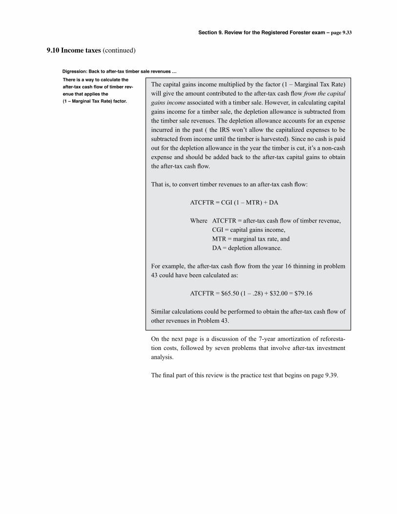
Section 9. Review for the Registered Forester exam – page 9.33
9.10 Income taxes (continued)
The capital gains income multiplied by the factor (1 – Marginal Tax Rate) will give the amount contributed to the after-tax cash flow from the capital gains income associated with a timber sale. However, in calculating capital gains income for a timber sale, the depletion allowance is subtracted from the timber sale revenues. The depletion allowance accounts for an expense incurred in the past ( the IRS won’t allow the capitalized expenses to be subtracted from income until the timber is harvested). Since no cash is paid out for the depletion allowance in the year the timber is cut, it’s a non-cash expense and should be added back to the after-tax capital gains to obtain the after-tax cash flow.
That is, to convert timber revenues to an after-tax cash flow:
ATCFTR = CGI (1 – MTR) + DA
Where ATCFTR = after-tax cash flow of timber revenue, CGI = capital gains income, MTR = marginal tax rate, and DA = depletion allowance.
For example, the after-tax cash flow from the year 16 thinning in problem 43 could have been calculated as:
ATCFTR = $65.50 (1 – .28) + $32.00 = $79.16
Similar calculations could be performed to obtain the after-tax cash flow of other revenues in Problem 43.
On the next page is a discussion of the 7-year amortization of reforesta-tion costs, followed by seven problems that involve after-tax investment analysis.
The final part of this review is the practice test that begins on page 9.39.
There is a way to calculate the after-tax cash flow of timber rev-enue that applies the (1 – Marginal Tax Rate) factor.
Digression: Back to after-tax timber sale revenues …
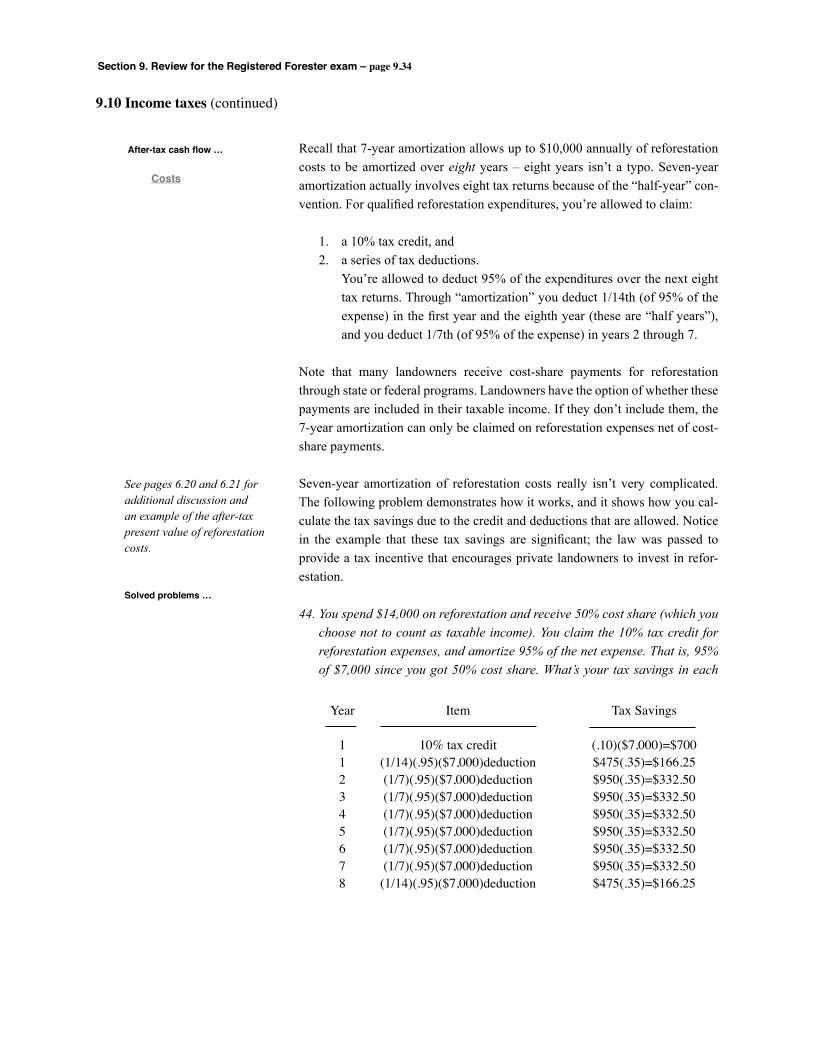
Section 9. Review for the Registered Forester exam – page 9.34
9.10 Income taxes (continued)
Recall that 7-year amortization allows up to $10,000 annually of reforestation costs to be amortized over eight years – eight years isn’t a typo. Seven-year amortization actually involves eight tax returns because of the “half-year” con-vention. For qualified reforestation expenditures, you’re allowed to claim:
1. a 10% tax credit, and 2. a series of tax deductions. You’re allowed to deduct 95% of the expenditures over the next eight
tax returns. Through “amortization” you deduct 1/14th (of 95% of the expense) in the first year and the eighth year (these are “half years”), and you deduct 1/7th (of 95% of the expense) in years 2 through 7.
Note that many landowners receive cost-share payments for reforestation through state or federal programs. Landowners have the option of whether these payments are included in their taxable income. If they don’t include them, the 7-year amortization can only be claimed on reforestation expenses net of cost-share payments.
Seven-year amortization of reforestation costs really isn’t very complicated. The following problem demonstrates how it works, and it shows how you cal-culate the tax savings due to the credit and deductions that are allowed. Notice in the example that these tax savings are significant; the law was passed to provide a tax incentive that encourages private landowners to invest in refor-estation.
44. You spend $14,000 on reforestation and receive 50% cost share (which you choose not to count as taxable income). You claim the 10% tax credit for reforestation expenses, and amortize 95% of the net expense. That is, 95% of $7,000 since you got 50% cost share. What’s your tax savings in each
After-tax cash flow …
Costs
Solved problems …
See pages 6.20 and 6.21 for additional discussion and an example of the after-tax present value of reforestation costs.
Year Item Tax Savings
1 10% tax credit (.10)($7,000)=$700 1 (1/14)(.95)($7,000)deduction $475(.35)=$166.25 2 (1/7)(.95)($7,000)deduction $950(.35)=$332.50 3 (1/7)(.95)($7,000)deduction $950(.35)=$332.50 4 (1/7)(.95)($7,000)deduction $950(.35)=$332.50 5 (1/7)(.95)($7,000)deduction $950(.35)=$332.50 6 (1/7)(.95)($7,000)deduction $950(.35)=$332.50 7 (1/7)(.95)($7,000)deduction $950(.35)=$332.50 8 (1/14)(.95)($7,000)deduction $475(.35)=$166.25
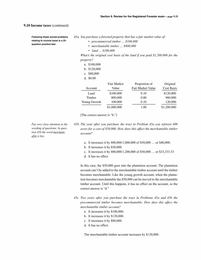
Section 9. Review for the Registered Forester exam – page 9.35
9.10 Income taxes (continued)
45a. You purchase a forested property that has a fair market value of: • precommercial timber … $100,000 • merchantable timber … $800,000 • land … $100,000 What’s the original cost basis of the land if you paid $1,200,000 for the
property? a. $100,000 b. $120,000 c. $80,000 d. $0.00
[The correct answer is “b.”]
45b. The year after you purchase the tract in Problem 45a you reforest 400 acres for a cost of $50,000. How does this affect the merchantable timber account?
a. It increases it by 800,000/1,000,000 of $50,000 … or $40,000. b. It increases it by $50,000. c. It increases it by 800,000/1,200,000 of $50,000 … or $33,333.33 d. It has no effect.
In this case, the $50,000 goes into the plantation account. The plantation account can’t be added to the merchantable timber account until the timber becomes merchantable. Like the young growth account, when the planta-tion becomes merchantable the $50,000 can be moved to the merchantable timber account. Until this happens, it has no effect on the account, so the correct answer is “d.”
45c. Two years after you purchase the tract in Problems 45a and 45b the precommercial timber becomes merchantable. How does this affect the merchantable timber account?
a. It increases it by $100,000. b. It increases it by $120,000. c. It increases it by $80,000. d. It has no effect. The merchantable timber account increases by $120,000.
Following these solved problems relating to income taxes is a 25-question practice test.
Pay very close attention to the wording of questions. In ques-tion 45b the word merchant-able is key.
Fair Market Proportion of Original Account Value Fair Market Value Cost Basis Land $100,000 0.10 $120,000 Timber 800,000 0.80 960,000 Young Growth 100,000 0.10 120,000 $1,000,000 1.00 $1,200,000

Section 9. Review for the Registered Forester exam – page 9.36
9.10 Income taxes (continued)
45d. Three years after you purchase the tract in Problems 45a, 45b, and 45c you sell half of the timber for $1,500,000. Your capital gains rate was 28%. How much tax is due on the sale?
a. $420,000 b. $302,000 c. $268,800 d. $151,200
Timber sale revenue = $1,500,000 Depletion allowance = (0.50)$1,080,000 = 540,000 Taxable capital gain = $960,000 Tax rate = .28 Income tax due = $268,800 [The correct answer is “c.”]
46. How much income tax is due on the following timber sale? Sale revenue = 2,000 MBF x $175/MBF = $350,000 Total merchantable volume, after the sale = 6,000 MBF Adjusted basis before the sale = $400,000 Capital gains tax rate = 28%
a. $98,000 b. $112,000 c. $70,000 d. $42,000
Timber sale revenue = $350,000 Depletion allowance = 2,000/8,000($400,000) = 100,000 Taxable capital gain = $250,000 Tax rate = .28 Income tax due = $70,000 [The correct answer is “c.”]
47. You attend a forestry shortcourse for business reasons. The cost of the course was $500, which in your case is tax deductible. If your marginal tax rate for ordinary income is 31%, what’s your after-tax cost of attend-ing the course?
The expense is fully deductible in the year incurred, so your after-tax cost is found by using the factor (1 – Tax Rate):
After-tax cost = $500 (1 – .31) = $345.00
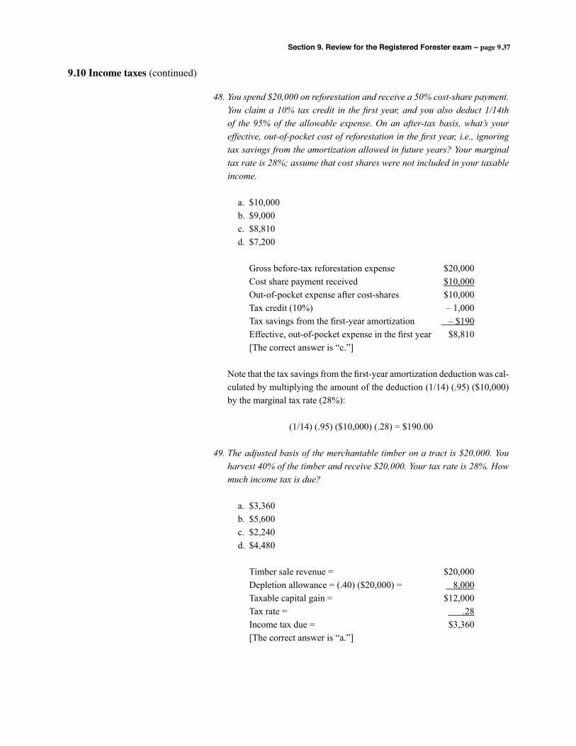
Section 9. Review for the Registered Forester exam – page 9.37
9.10 Income taxes (continued)
48. You spend $20,000 on reforestation and receive a 50% cost-share payment. You claim a 10% tax credit in the first year, and you also deduct 1/14th of the 95% of the allowable expense. On an after-tax basis, what’s your effective, out-of-pocket cost of reforestation in the first year, i.e., ignoring tax savings from the amortization allowed in future years? Your marginal tax rate is 28%; assume that cost shares were not included in your taxable income.
a. $10,000 b. $9,000 c. $8,810 d. $7,200
Gross before-tax reforestation expense $20,000 Cost share payment received $10,000 Out-of-pocket expense after cost-shares $10,000 Tax credit (10%) – 1,000 Tax savings from the first-year amortization – $190 Effective, out-of-pocket expense in the first year $8,810 [The correct answer is “c.”]
Note that the tax savings from the first-year amortization deduction was cal-culated by multiplying the amount of the deduction (1/14) (.95) ($10,000) by the marginal tax rate (28%):
(1/14) (.95) ($10,000) (.28) = $190.00
49. The adjusted basis of the merchantable timber on a tract is $20,000. You harvest 40% of the timber and receive $20,000. Your tax rate is 28%. How much income tax is due?
a. $3,360 b. $5,600 c. $2,240 d. $4,480
Timber sale revenue = $20,000 Depletion allowance = (.40) ($20,000) = 8,000 Taxable capital gain = $12,000 Tax rate = .28 Income tax due = $3,360 [The correct answer is “a.”]
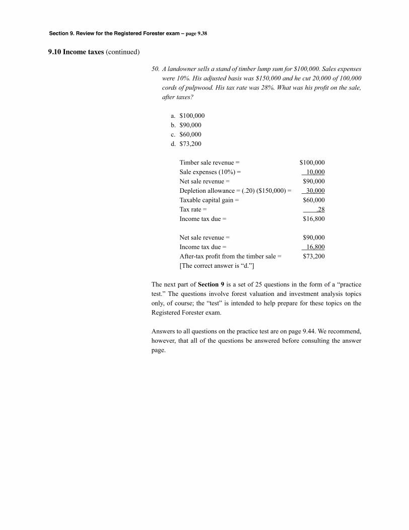
Section 9. Review for the Registered Forester exam – page 9.38
9.10 Income taxes (continued)
50. A landowner sells a stand of timber lump sum for $100,000. Sales expenses were 10%. His adjusted basis was $150,000 and he cut 20,000 of 100,000 cords of pulpwood. His tax rate was 28%. What was his profit on the sale, after taxes?
a. $100,000 b. $90,000 c. $60,000 d. $73,200
Timber sale revenue = $100,000 Sale expenses (10%) = 10,000 Net sale revenue = $90,000 Depletion allowance = (.20) ($150,000) = 30,000 Taxable capital gain = $60,000 Tax rate = .28 Income tax due = $16,800
Net sale revenue = $90,000 Income tax due = 16,800 After-tax profit from the timber sale = $73,200 [The correct answer is “d.”]
The next part of Section 9 is a set of 25 questions in the form of a “practice test.” The questions involve forest valuation and investment analysis topics only, of course; the “test” is intended to help prepare for these topics on the Registered Forester exam.
Answers to all questions on the practice test are on page 9.44. We recommend, however, that all of the questions be answered before consulting the answer page.
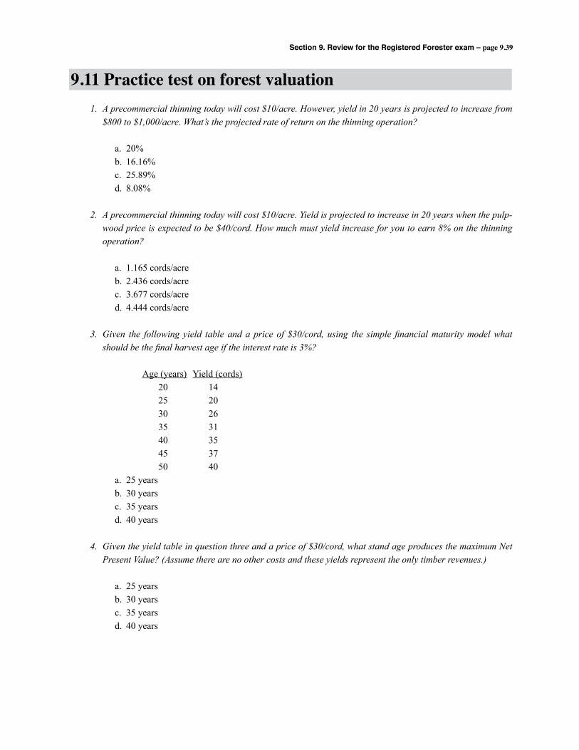
Section 9. Review for the Registered Forester exam – page 9.39
9.11 Practice test on forest valuation1. A precommercial thinning today will cost $10/acre. However, yield in 20 years is projected to increase from
$800 to $1,000/acre. What’s the projected rate of return on the thinning operation?
a. 20% b. 16.16% c. 25.89% d. 8.08%
2. A precommercial thinning today will cost $10/acre. Yield is projected to increase in 20 years when the pulp-wood price is expected to be $40/cord. How much must yield increase for you to earn 8% on the thinning operation?
a. 1.165 cords/acre b. 2.436 cords/acre c. 3.677 cords/acre d. 4.444 cords/acre
3. Given the following yield table and a price of $30/cord, using the simple financial maturity model what should be the final harvest age if the interest rate is 3%?
Age (years) Yield (cords) 20 14 25 20 30 26 35 31 40 35 45 37 50 40 a. 25 years b. 30 years c. 35 years d. 40 years
4. Given the yield table in question three and a price of $30/cord, what stand age produces the maximum Net Present Value? (Assume there are no other costs and these yields represent the only timber revenues.)
a. 25 years b. 30 years c. 35 years d. 40 years
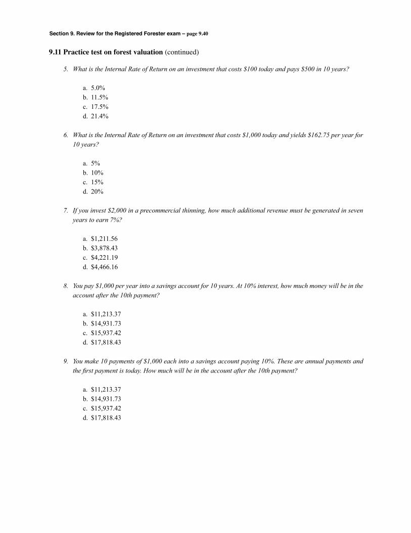
Section 9. Review for the Registered Forester exam – page 9.40
9.11 Practice test on forest valuation (continued)
5. What is the Internal Rate of Return on an investment that costs $100 today and pays $500 in 10 years?
a. 5.0% b. 11.5% c. 17.5% d. 21.4%
6. What is the Internal Rate of Return on an investment that costs $1,000 today and yields $162.75 per year for 10 years?
a. 5% b. 10% c. 15% d. 20%
7. If you invest $2,000 in a precommercial thinning, how much additional revenue must be generated in seven years to earn 7%?
a. $1,211.56 b. $3,878.43 c. $4,221.19 d. $4,466.16
8. You pay $1,000 per year into a savings account for 10 years. At 10% interest, how much money will be in the account after the 10th payment?
a. $11,213.37 b. $14,931.73 c. $15,937.42 d. $17,818.43
9. You make 10 payments of $1,000 each into a savings account paying 10%. These are annual payments and the first payment is today. How much will be in the account after the 10th payment?
a. $11,213.37 b. $14,931.73 c. $15,937.42 d. $17,818.43
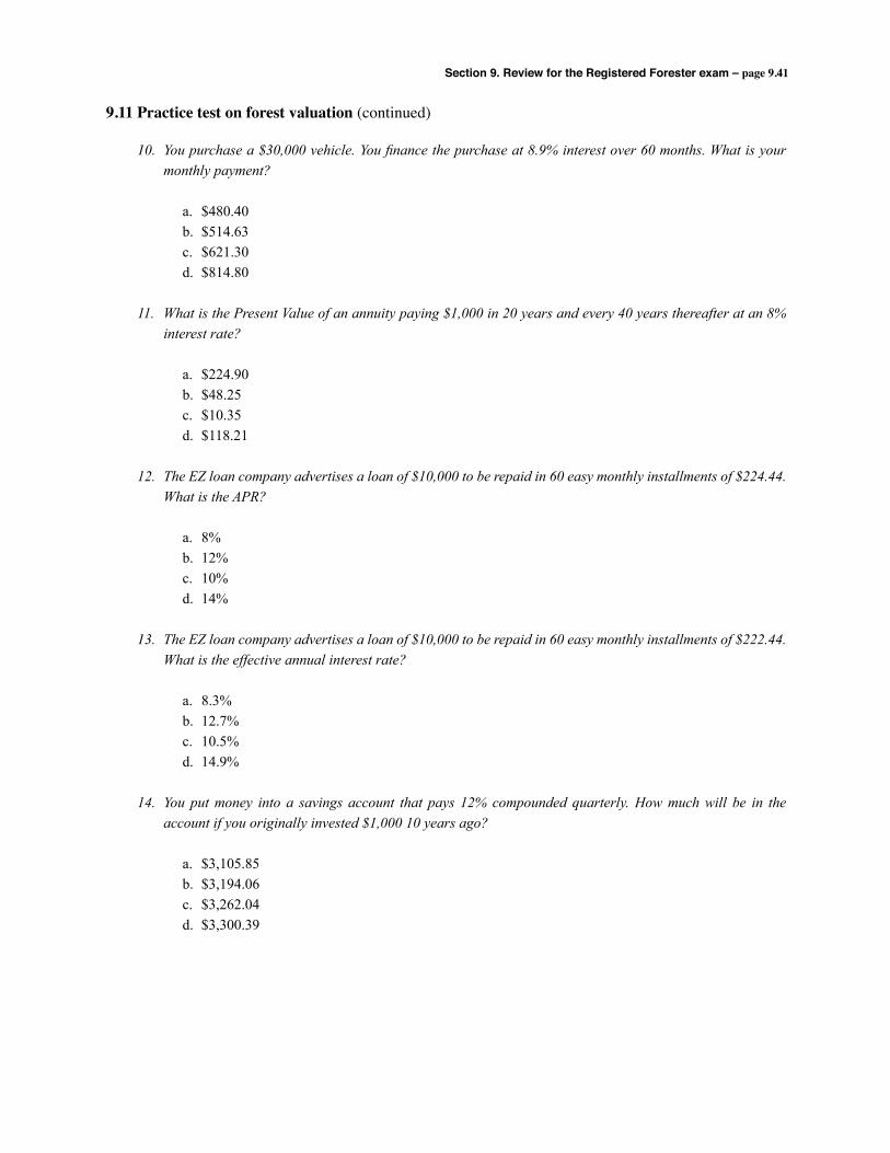
Section 9. Review for the Registered Forester exam – page 9.41
9.11 Practice test on forest valuation (continued)
10. You purchase a $30,000 vehicle. You finance the purchase at 8.9% interest over 60 months. What is your monthly payment?
a. $480.40 b. $514.63 c. $621.30 d. $814.80
11. What is the Present Value of an annuity paying $1,000 in 20 years and every 40 years thereafter at an 8% interest rate?
a. $224.90 b. $48.25 c. $10.35 d. $118.21
12. The EZ loan company advertises a loan of $10,000 to be repaid in 60 easy monthly installments of $224.44. What is the APR?
a. 8% b. 12% c. 10% d. 14%
13. The EZ loan company advertises a loan of $10,000 to be repaid in 60 easy monthly installments of $222.44. What is the effective annual interest rate?
a. 8.3% b. 12.7% c. 10.5% d. 14.9%
14. You put money into a savings account that pays 12% compounded quarterly. How much will be in the account if you originally invested $1,000 10 years ago?
a. $3,105.85 b. $3,194.06 c. $3,262.04 d. $3,300.39
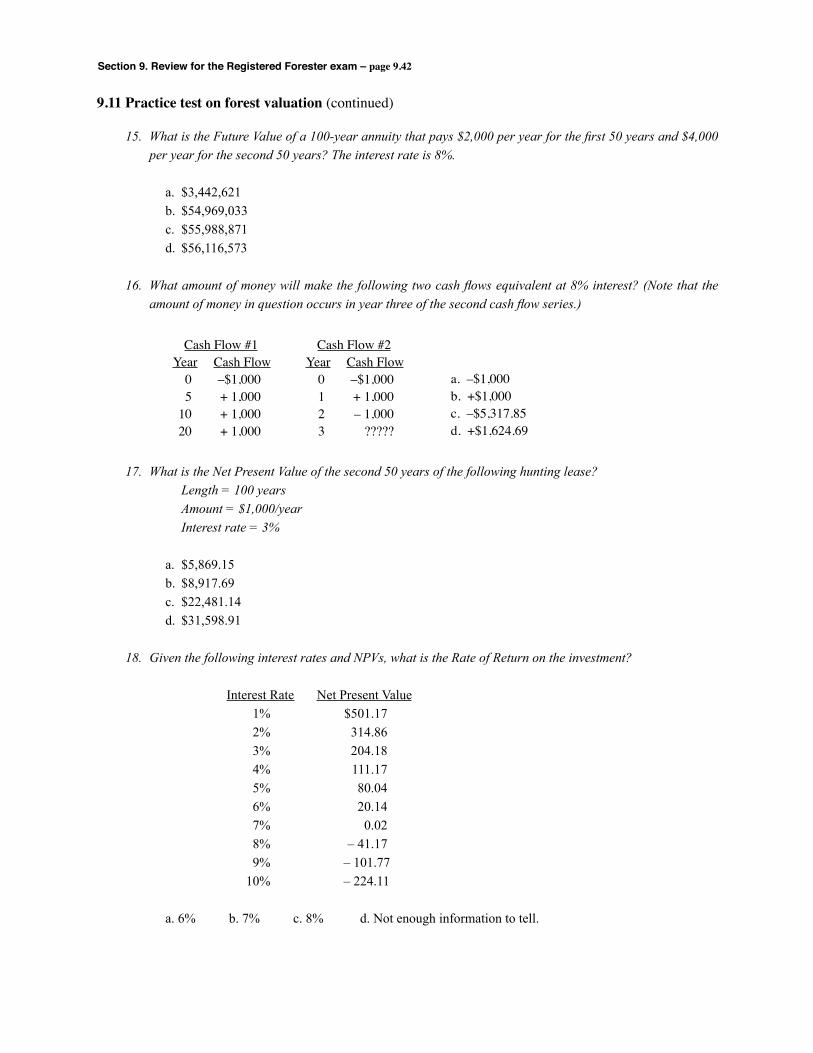
Section 9. Review for the Registered Forester exam – page 9.42
9.11 Practice test on forest valuation (continued)
15. What is the Future Value of a 100-year annuity that pays $2,000 per year for the first 50 years and $4,000 per year for the second 50 years? The interest rate is 8%.
a. $3,442,621 b. $54,969,033 c. $55,988,871 d. $56,116,573
16. What amount of money will make the following two cash flows equivalent at 8% interest? (Note that the amount of money in question occurs in year three of the second cash flow series.)
17. What is the Net Present Value of the second 50 years of the following hunting lease? Length = 100 years Amount = $1,000/year Interest rate = 3%
a. $5,869.15 b. $8,917.69 c. $22,481.14 d. $31,598.91
18. Given the following interest rates and NPVs, what is the Rate of Return on the investment?
Interest Rate Net Present Value 1% $501.17 2% 314.86 3% 204.18 4% 111.17 5% 80.04 6% 20.14 7% 0.02 8% – 41.17 9% – 101.77 10% – 224.11
a. 6% b. 7% c. 8% d. Not enough information to tell.
Cash Flow #1 Year Cash Flow 0 –$1,000 5 + 1,000 10 + 1,000 20 + 1,000
Cash Flow #2 Year Cash Flow 0 –$1,000 1 + 1,000 2 – 1,000 3 ?????
a. –$1,000b. +$1,000c. –$5,317.85d. +$1,624.69

Section 9. Review for the Registered Forester exam – page 9.43
9.11 Practice test on forest valuation (continued)
19. What is the Net Present Value of the following cash flow at 8%? The cash flow is perpetual.
a. $1,250.00 b. $1,350.00 c. $2,551.92 d. $1,999.04
20. Assume inflation has averaged 5% over the last 10 years and the price of hardwood pulpwood has risen 5% annually in real terms over the same period. If the price was $5/cord 10 years ago, what is it today?
a. $7.50/cord b. $13.27/cord c. $8.14/cord d. $10.00/cord
21. You place $1,000 in a savings account paying 10% annually. How much interest will you earn the third year?
a. $100.00 b. $210.00 c. $121.00 d. $331.00
22. You perform a timber stand improvement operation that cost $10/acre. This was an “ordinary expense” for income tax purposes. If your marginal tax rate was 35%, what was your after-tax cost?
a. $3.50 b. $10.00 c. $6.50 d. $13.50
23. You purchase a timber tract for $25,000 and sell it in eight years for $50,000. Your capital gains tax rate is 28%. What is your after-tax Rate of Return?
a. 7% b. 9.1% c. 8.4% d. 9.9%
0 1 2 3 4 5 6 7 8 9 10
$100
$100
$100
$100
$100
$100
$200 $2
00 $200 $2
00$2
00
8
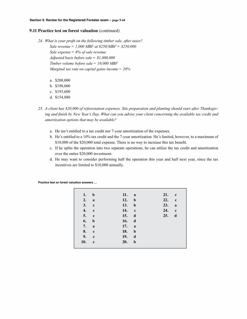
Section 9. Review for the Registered Forester exam – page 9.44
9.11 Practice test on forest valuation (continued)
24. What is your profit on the following timber sale, after taxes? Sale revenue = 1,000 MBF at $250/MBF = $250,000 Sale expense = 8% of sale revenue Adjusted basis before sale = $1,000,000 Timber volume before sale = 10,000 MBF Marginal tax rate on capital gains income = 28%
a. $208,000 b. $198,000 c. $193,600 d. $154,880
25. A client has $20,000 of reforestation expenses. Site preparation and planting should start after Thanksgiv-ing and finish by New Year’s Day. What can you advise your client concerning the available tax credit and amortization options that may be available?
a. He isn’t entitled to a tax credit nor 7-year amortization of the expenses. b. He’s entitled to a 10% tax credit and the 7-year amortization. He’s limited, however, to a maximum of
$10,000 of the $20,000 total expense. There is no way to increase this tax benefit. c. If he splits the operation into two separate operations, he can utilize the tax credit and amortization
over the entire $20,000 investment. d. He may want to consider performing half the operation this year and half next year, since the tax
incentives are limited to $10,000 annually.
Practice test on forest valuation answers …
1. b 11. a 21. c 2. a 12. b 22. c 3. c 13. b 23. a 4. c 14. c 24. c 5. c 15. d 25. d 6. b 16. d 7. a 17. a 8. c 18. b 9. c 19. d 10. c 20. b
Section 9. Review for the Registered Forester exam – page 9.45
9.12 Timber production relationships in forest management
Growth and yield prediction is fundamental to forest resource management. Basic timber production relationships are often included in the forest manage-ment section of the Registered Forester exam. Sections 9.12 through 9.14 cover material that relate to forest resource management. Section 9.15 is a practice test covering that material.
Mean annual increment (MAI) is the average growth of a stand at a specified age.
where: MAI = mean annual increment YA = yield at stand age “A”
Periodic annual increment (PAI) is average growth of a stand over a specified time period (specified by the yield table interval). Current annual increment (CAI) is a special case of PAI where the time interval is one year (i.e., the yield table has yields at all ages). So CAI is growth from year to year.
where: PAI = periodic annual increment A = stand age n = interval between stand age in the yield table Y = yield at specified stand age
51. Consider the following yield table with a 5-year interval. Calculate MAI and PAI. Note that PAI is usually listed between stand ages (because it is average growth between these ages). It would also be plotted this way.
This Section is a review of basic timber production topics, includ-ing stand density measures and site quality concepts.
MAI =YA
A
PAI =YA + n – YA
n
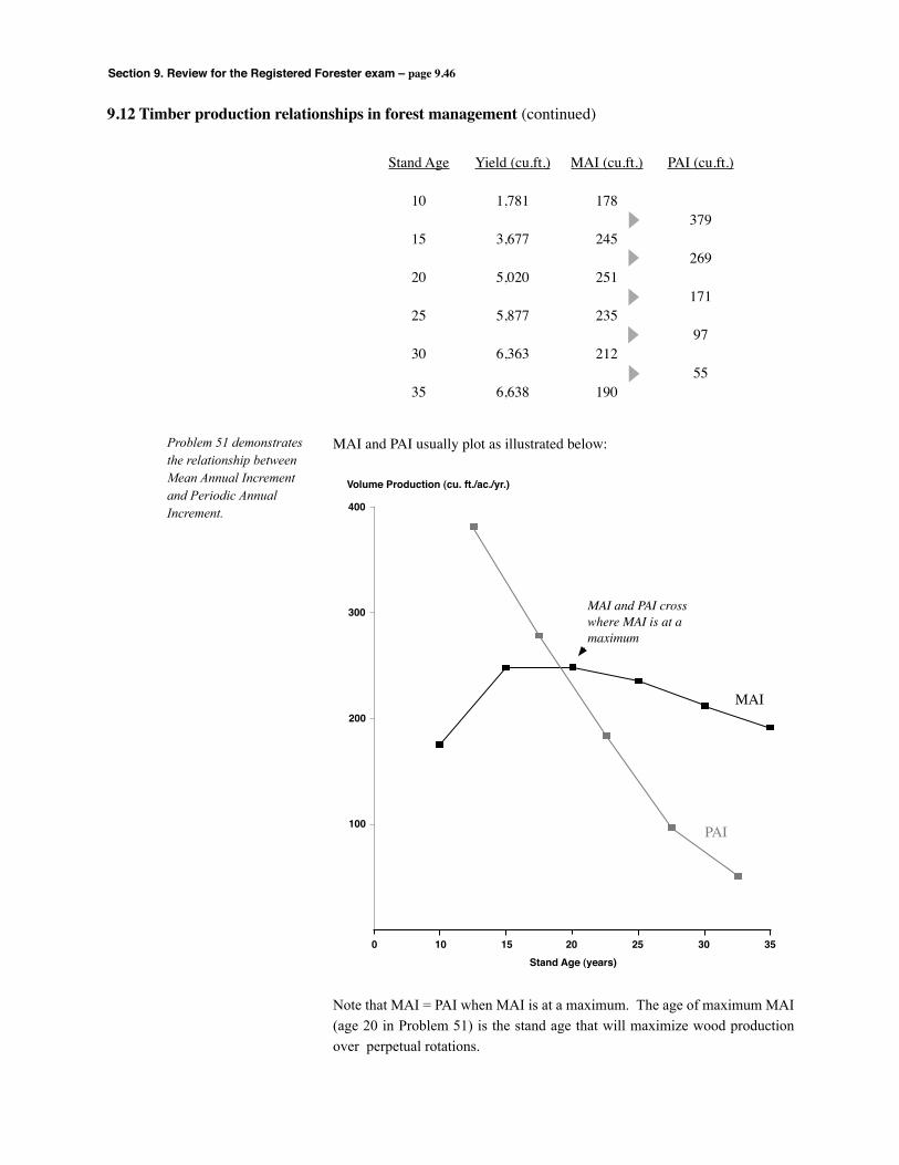
Section 9. Review for the Registered Forester exam – page 9.46
9.12 Timber production relationships in forest management (continued)
Stand Age
10
15
20
25
30
35
Yield (cu.ft.)
1,781
3,677
5,020
5,877
6,363
6,638
MAI (cu.ft.)
178
245
251
235
212
190
PAI (cu.ft.)
379
269
171
97
55
MAI and PAI usually plot as illustrated below:Problem 51 demonstrates the relationship between Mean Annual Increment and Periodic Annual Increment.
MAI
PAI
MAI and PAI cross where MAI is at amaximum
400
300
200
100
0 10 15 20 25 30 35
Volume Production (cu. ft./ac./yr.)
Stand Age (years)
Note that MAI = PAI when MAI is at a maximum. The age of maximum MAI (age 20 in Problem 51) is the stand age that will maximize wood production over perpetual rotations.
Section 9. Review for the Registered Forester exam – page 9.47
9.12 Timber production relationships in forest management (continued)
52. The age of maximum MAI for a loblolly pine stand is 23 years. Maximum MAI = 238 cu.ft./ac./yr. at age 23 years. What is PAI at age 23?
a. 238 cu.ft./ac./yr. b. less than 238 cu.ft./ac./yr. c. more than 238 cu.ft./ac./yr. d. not enough information to tell
The answer is “a” since MAI = PAI at the age of maximum MAI.
Two factors primarily determine the timber actually produced on a tract of land during a given time period: site quality (the productive potential of the land to grow timber) and the distribution (by size, species, spatial pattern, age, etc.) of the growing stock currently on the site.
Stand density measures quantitatively the extent of stem crowding within a given area. Stocking, while often related to density, is a qualitative measure. Stocking compares the existing number of trees in a stand to the number desired for optimum growth and volume. Stands are often referred to as fully-stocked (or 100% stocked), over-stocked, or under-stocked.
Example: A stand contains 300 trees per acre. Originally, 400 trees per acre were
planted; for optimum growth 375 trees per acre are desired. The stand density is 300 trees per acre. The stand is under-stocked or 80% stocked. Percent Survival is 75 percent.
The basic relationship that makes stand density important is that, within limits, the more growing space a tree has, the faster it will grow. Thus, a primary means for a forester to control stand growth and tree characteristics is to control stand density by thinning and other silvicultural means.
How does density affect stand structure? Height growth is little affected by stand density – that’s part of the reason stand height is used to predict site quality. Diameter growth, however, is strongly correlated with stand density. Basal area is affected by stand density in the early years of stand development; but in later development, all stands move toward basal area carrying capacity. Mortality is closely related to stand density. These relationships are illustrated on the following page.
Stand density and site qual-ity are extremely important in timber production on a specific tract of land.
Solved problem …

Section 9. Review for the Registered Forester exam – page 9.48
9.12 Timber production relationships in forest management (continued)
Height growth is not greatly affected by stand density. This fact is an important assumption in the “site index” discussion on page 9.58, since tree height growth is nearly independent of den-sity, we don’t need different site index curves for various stand densities.
Diameter growth is strongly correlated with stand density.
Decreasing stand density produces significant increases in diameter growth at breast height.
Basal area is a measure of stand density (see page 9.49); in the early years of stand develop-ment, the wider planting spacings result in lower stand basal areas.
Basal area for all three initial spacings moves to the site’s carrying capacity (of about 200 square feet per acre). An important question is “While all three sites are fully occupied, what are the differences in tree characteristics in the three stands?”
Mortality is closely related to the carrying capac-ity of the site; note that all three spacings are moving to a relatively equal density by age 30.
The closer the initial spacing, the greater the mortality over time.
a) Height
b) Diameter
c) Basal Area
d) Survival
The diagrams below show fundamental relationships between stand density (planting spacing) and stand attributes. The diagrams are based on data for loblolly pine plantations. They were adapted from Conrad, L.W. III, T.J. Straka, and W.F. Watson. 1992. Economic evaluation of initial spacing for a thirty-year-old unthinned loblolly pine plantation. South. J. Appl. For. 16(2):89-93.
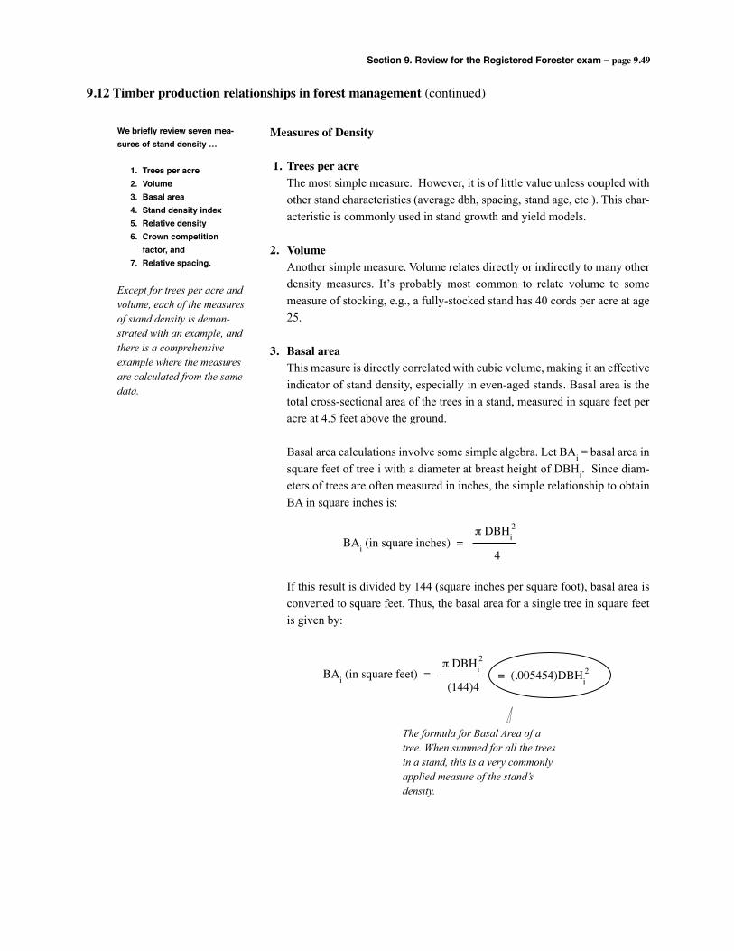
Section 9. Review for the Registered Forester exam – page 9.49
9.12 Timber production relationships in forest management (continued)
We briefly review seven mea-sures of stand density …
1. Trees per acre 2. Volume 3. Basal area 4. Stand density index 5. Relative density 6. Crown competition factor, and 7. Relative spacing.
Except for trees per acre and volume, each of the measures of stand density is demon-strated with an example, and there is a comprehensive example where the measures are calculated from the same data.
Measures of Density
1. Trees per acre The most simple measure. However, it is of little value unless coupled with
other stand characteristics (average dbh, spacing, stand age, etc.). This char-acteristic is commonly used in stand growth and yield models.
2. Volume Another simple measure. Volume relates directly or indirectly to many other
density measures. It’s probably most common to relate volume to some measure of stocking, e.g., a fully-stocked stand has 40 cords per acre at age 25.
3. Basal area This measure is directly correlated with cubic volume, making it an effective
indicator of stand density, especially in even-aged stands. Basal area is the total cross-sectional area of the trees in a stand, measured in square feet per acre at 4.5 feet above the ground.
Basal area calculations involve some simple algebra. Let BAi = basal area in square feet of tree i with a diameter at breast height of DBHi. Since diam-eters of trees are often measured in inches, the simple relationship to obtain BA in square inches is:
If this result is divided by 144 (square inches per square foot), basal area is converted to square feet. Thus, the basal area for a single tree in square feet is given by:
BAi (in square inches) =π DBHi
2
4
BAi (in square feet) =π DBHi
2
(144)4= (.005454)DBHi
2
The formula for Basal Area of a tree. When summed for all the trees in a stand, this is a very commonly applied measure of the stand’s density.
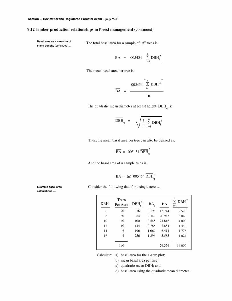
Section 9. Review for the Registered Forester exam – page 9.50
9.12 Timber production relationships in forest management (continued)
Basal area as a measure of stand density (continued) …
The total basal area for a sample of “n” trees is:
BA = .005454 DBHi2∑
i=1
n
The mean basal area per tree is:
.005454 DBHi2∑
i=1
n
BA = n
The quadratic mean diameter at breast height, DBHq is:
DBHq = DBHi21
n∑i=1
n
Thus, the mean basal area per tree can also be defined as:
BA = .005454 DBHq2
And the basal area of n sample trees is:
BA = (n) .005454 DBHq
2
Consider the following data for a single acre …
68
10121416
7060401064
190
3664
100144196256
0.1960.3490.5450.7851.0691.396
13.74420.94321.8167.8546.4145.585
76.356
2,5203,8404,0001,4401,7761,024
14,000
TreesPer AcreDBHi DBHi
2 BAi BA DBHi2∑
i=1
n
Calculate: a) basal area for the 1-acre plot; b) mean basal area per tree; c) quadratic mean DBH; and d) basal area using the quadratic mean diameter.
Example basal area calculations …
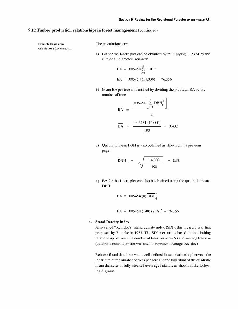
Section 9. Review for the Registered Forester exam – page 9.51
9.12 Timber production relationships in forest management (continued)
Example basal area calculations (continued) …
The calculations are:
a) BA for the 1-acre plot can be obtained by multiplying .005454 by the sum of all diameters squared:
BA = .005454 ∑ DBHi
BA = .005454 (14,000) = 76.356
b) Mean BA per tree is identified by dividing the plot total BA by the number of trees:
c) Quadratic mean DBH is also obtained as shown on the previous page:
d) BA for the 1-acre plot can also be obtained using the quadratic mean DBH:
BA = .005454 (n) DBHq
BA = .005454 (190) (8.58)2 = 76.356
4. Stand Density Index Also called “Reineke’s” stand density index (SDI), this measure was first
proposed by Reineke in 1933. The SDI measure is based on the limiting relationship between the number of trees per acre (N) and average tree size (quadratic mean diameter was used to represent average tree size).
Reineke found that there was a well-defined linear relationship between the logarithm of the number of trees per acre and the logarithm of the quadratic mean diameter in fully-stocked even-aged stands, as shown in the follow-ing diagram.
2
i=1
n
.005454 DBHi2∑
i=1
n
BA = n
.005454 (14,000)BA = = 0.402
190
DBHq = = 8.58 14,000
190
2
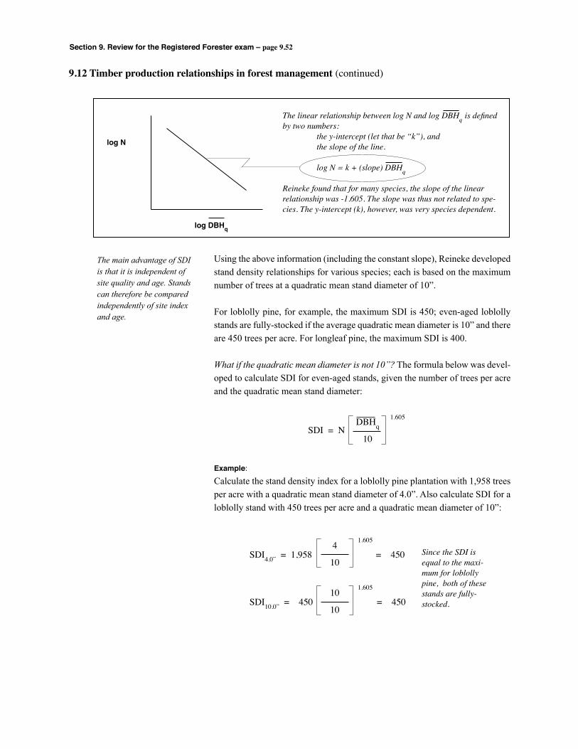
Section 9. Review for the Registered Forester exam – page 9.52
9.12 Timber production relationships in forest management (continued)
The main advantage of SDI is that it is independent of site quality and age. Stands can therefore be compared independently of site index and age.
Using the above information (including the constant slope), Reineke developed stand density relationships for various species; each is based on the maximum number of trees at a quadratic mean stand diameter of 10”.
For loblolly pine, for example, the maximum SDI is 450; even-aged loblolly stands are fully-stocked if the average quadratic mean diameter is 10” and there are 450 trees per acre. For longleaf pine, the maximum SDI is 400.
What if the quadratic mean diameter is not 10”? The formula below was devel-oped to calculate SDI for even-aged stands, given the number of trees per acre and the quadratic mean stand diameter:
Example:Calculate the stand density index for a loblolly pine plantation with 1,958 trees per acre with a quadratic mean stand diameter of 4.0”. Also calculate SDI for a loblolly stand with 450 trees per acre and a quadratic mean diameter of 10”:
log N
log DBHq
The linear relationship between log N and log DBHq is defined by two numbers: the y-intercept (let that be “k”), and the slope of the line.
log N = k + (slope) DBHq
Reineke found that for many species, the slope of the linear relationship was -1.605. The slope was thus not related to spe-cies. The y-intercept (k), however, was very species dependent.
SDI = NDBHq
10
1.605
SDI4.0” = 1,958 = 4504
10
1.605
SDI10.0” = 450 = 45010
10
1.605
Since the SDI is equal to the maxi-mum for loblolly pine, both of these stands are fully-stocked.
Section 9. Review for the Registered Forester exam – page 9.53
9.12 Timber production relationships in forest management (continued)
We briefly review seven mea-sures of stand density …
1. Trees per acre 2. Volume 3. Basal area 4. Stand density index 5. Relative density 6. Crown competition factor, and 7. Relative spacing.
5. Relative Density Relative density (RD) is a common measure of stand density in the Pacific
Northwest. RD is defined as:
Generally, relative densities in the lower 20s characterize open-grown stands, a stand with a relative density of 50 is a candidate for thinning, and a relative density in the 60s is overstocked.
Example: For the example loblolly pine plantation on the previous page (N = 1,958
and quadratic mean diameter = 4.0”), we can calculate relative density as:
BA = .005454 (1,958) (4.02) = 170.86
Since the SDI for this stand is at the limiting number of trees per acre (see the SDI example on the previous page), our RD result is consistent – it indi-cates full (or over) stocking.
DBHq
BARD =
Basal Area(see page 9.49)
Quadratic mean diameter(see page 9.50)
170.86RD = = 85.43
4
Section 9. Review for the Registered Forester exam – page 9.54
9.12 Timber production relationships in forest management (continued)
Crown Competition Factor … 6. Crown Competition Factor The relationship between crown width (CW) and the diameter of a tree can
be estimated by a linear function:
CW = β0 + β1D … where CW is in feet and D is in inches
Since CW is in feet, the formula for the area of a circle yields estimated crown area (CA) in square feet:
CA = (CW)2
Or, substituting for CW,
CA = (β0 + β1D)2
The maximum crown area (MCA) that an open-grown tree (of diameter D) can occupy, expressed as a percentage of an acre, is:
MCA =
Simplifying the equation yields:
MCA = 0.001803 (β0 + β1D)2
Crown competition factor (CCF) is the sum of MCA for all the trees in a stand, expressed on a per acre basis.
Example: An ordinary least squares regression where crown width was predicted as
a function of diameter produced the following estimated values for β0 and β1:
CW = 4.0 + 2.5 (D)
Therefore,
MCA = 0.001803 (4.0 + 2.5 D)2
MCA = 0.001803 (6.25 D2 + 20 D + 16) MCA = 0.01127 D2 + 0.0306 D + 0.02885
π
4
π
4
(β0 + β
1D)2 100π
443,560
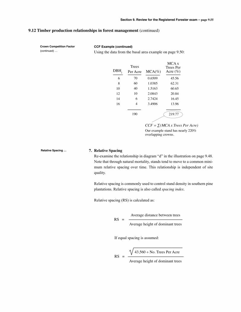
Section 9. Review for the Registered Forester exam – page 9.55
9.12 Timber production relationships in forest management (continued)
Crown Competition Factor (continued) …
CCF Example (continued) Using the data from the basal area example on page 9.50:
68
10121416
7060401064
190
0.65091.03851.51632.08432.74243.4906
TreesPer AcreDBHi MCA(%)
45.5662.3160.6520.8416.4513.96
219.77
MCA xTrees PerAcre (%)
CCF = ∑(MCA x Trees Per Acre)Our example stand has nearly 220% overlapping crowns.
7. Relative Spacing Re-examine the relationship in diagram “d” in the illustration on page 9.48.
Note that through natural mortality, stands tend to move to a common mini-mum relative spacing over time. This relationship is independent of site quality.
Relative spacing is commonly used to control stand density in southern pine plantations. Relative spacing is also called spacing index.
Relative spacing (RS) is calculated as:
Relative Spacing …
RS =Average distance between trees
Average height of dominant trees
If equal spacing is assumed:
RS =43,560 ÷ No. Trees Per Acre
Average height of dominant trees

Section 9. Review for the Registered Forester exam – page 9.56
9.12 Timber production relationships in forest management (continued)
Relative Spacing Example A pine plantation has 250 trees per acre with an average dominant height of
90 feet. Assuming equal spacing,
Relative spacing is often used to specify thinning regimes. Suppose a thin-ning regime involves two thinnings, one when dominant height is 40 feet and the second thinning when dominant height is 80 feet. A relative spacing of 0.20 is specified. What number of trees should be remaining after the first and second thinnings?
After the first thinning:
N = 43,560 ÷ (40 x 0.20)2 = 681 trees per acre
After the second thinning:
N = 43,560 ÷ (80 x 0.20)2 = 170 trees per acre
Solved problems:53. You measure the 10 loblolly pine trees below on a 1/10th acre plot. What are
the average and quadratic mean diameters. What is the basal area of the plot?
Relative Spacing (continued) …
RS = 43,560 ÷ 250
90
TreeNo.
123456789
10
DBH(in.)
666688
1010121486
DBH2
363636366464
100100144196812
BA(sq.ft.)0.19630.19630.19630.19630.34910.34910.54540.54540.78541.0690
4.42856
Basal Area on the plot = 4.4286 sq. ft.
DBH = = 8.6”
DBHq = = 9.0”
8610
812 / 10
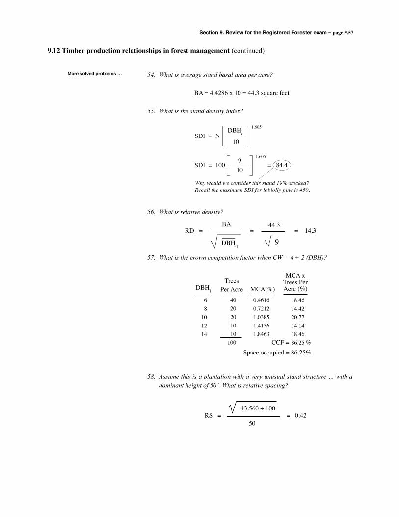
Section 9. Review for the Registered Forester exam – page 9.57
9.12 Timber production relationships in forest management (continued)
54. What is average stand basal area per acre?
BA = 4.4286 x 10 = 44.3 square feet
55. What is the stand density index?
56. What is relative density?
57. What is the crown competition factor when CW = 4 + 2 (DBH)?
58. Assume this is a plantation with a very unusual stand structure … with a dominant height of 50’. What is relative spacing?
More solved problems …
RS = = 0.42 43,560 ÷ 100
50
SDI = NDBHq
10
1.605
SDI = 100 = 84.4910
1.605
Why would we consider this stand 19% stocked?Recall the maximum SDI for loblolly pine is 450.
DBHq
BARD = = = 14.3
9
44.3
68
101214
4020201010
100
0.46160.72121.03851.41361.8463
TreesPer AcreDBHi MCA(%)
18.4614.4220.7714.1418.4686.25
MCA xTrees PerAcre (%)
CCF = %Space occupied = 86.25%
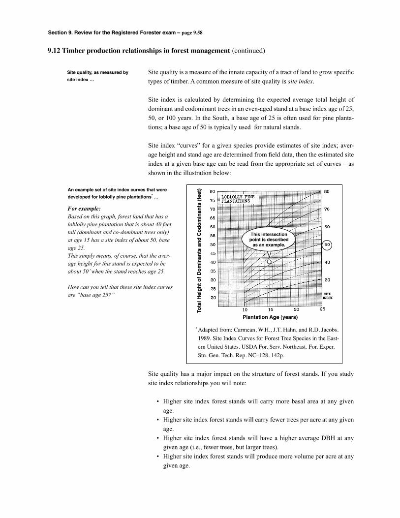
Section 9. Review for the Registered Forester exam – page 9.58
9.12 Timber production relationships in forest management (continued)
Site quality is a measure of the innate capacity of a tract of land to grow specific types of timber. A common measure of site quality is site index.
Site index is calculated by determining the expected average total height of dominant and codominant trees in an even-aged stand at a base index age of 25, 50, or 100 years. In the South, a base age of 25 is often used for pine planta-tions; a base age of 50 is typically used for natural stands.
Site index “curves” for a given species provide estimates of site index; aver-age height and stand age are determined from field data, then the estimated site index at a given base age can be read from the appropriate set of curves – as shown in the illustration below:
Site quality, as measured by site index …
Site quality has a major impact on the structure of forest stands. If you study site index relationships you will note:
• Higher site index forest stands will carry more basal area at any given age.
• Higher site index forest stands will carry fewer trees per acre at any given age.
• Higher site index forest stands will have a higher average DBH at any given age (i.e., fewer trees, but larger trees).
• Higher site index forest stands will produce more volume per acre at any given age.
Adapted from: Carmean, W.H., J.T. Hahn, and R.D. Jacobs. 1989. Site Index Curves for Forest Tree Species in the East-ern United States. USDA For. Serv. Northeast. For. Exper. Stn. Gen. Tech. Rep. NC–128, 142p.
Tota
l Hei
ght o
f Dom
inan
ts a
nd C
odom
inan
ts (f
eet)
Plantation Age (years)
For example:Based on this graph, forest land that has a loblolly pine plantation that is about 40 feet tall (dominant and co-dominant trees only) at age 15 has a site index of about 50, base age 25.This simply means, of course, that the aver-age height for this stand is expected to be about 50’ when the stand reaches age 25.
How can you tell that these site index curves are “base age 25?”
An example set of site index curves that were developed for loblolly pine plantations* …
*
This intersectionpoint is described
as an example.
Section 9. Review for the Registered Forester exam – page 9.59
What’s a “fully-regulated” forest?The classical forest regulation model defines a fully-regulated forest as one with age and size classes of trees such that the forest yields approximately equal quantities of desired forest products on a periodic basis. Early literature refers to fully-regulated forests as “normal” forests. The concept goes back to the European roots of American forestry that stressed a continuous even-flow of timber products.
What’s a “normal” forest?A normal forest is an interesting theoretical model. It presents an interesting starting point in discussing fully-regulated forests. A normal forest represents the traditional “textbook” model of a fully-regulated forest.
The normal forest concept involves simple assumptions:
• All forest stands are fully-stocked, i.e., “normal” growing stock levels exist in all stands.
• Equal site productivity and management intensity occur across the forest.
• The age-class distribution includes stands of equal acreage represent-ing each age class to the rotation age. If maximum wood production is required over time, the rotation age equals the age of maximum mean annual increment.
The fully-regulated even-aged forest…The “normal” forest described above provides an excellent starting point for discussing forest regulation. By definition, all normal forests are regulated. Of course not all fully-regulated forests are normal forests.
In the normal forest, we will assume a constant site productivity, a single timber species, and one management regime. Each age class represents a single stand. Each year, the oldest age class (the age class equal to the rotation age) is har-vested. This stand then becomes the youngest age class. The forest has a con-stant structure.
If the rotation age and total acres are known, the number of acres in each age class is given by:
9.15 Classical forest regulation
Four techniques forestablishing a fully-regulated forest over time … 1. Growing stock 2. Annual harvest 3. Volume control 4. Equivalent acres
Acres ineach ageclass (a)
Total acreage in the forest (A)
Rotation Age (R)=
Or, a =A
R

Section 9. Review for the Registered Forester exam – page 9.60
9.13 Classical forest regulation (continued)
Solved problem:59. Assume we want to maximize mean annual increment and the following
yield table is appropriate for our loblolly pine forest. Our pulpwood rota-tion would be 25 years (maximum mean annual increment equals 2.64 cords per acre per year at age 25).
Example YieldsAge
(years)789
1011121314151617181920212223242526
Yield(cords/ac.)
1247
10152025303540444851545760636668
If the total area of the forest is 500,000 acres, the area per age class is:
a =A
R=
500,000 acres
25 years
The 25 age classes in this fully-regulated forest are illustrated in the diagram on the next page.
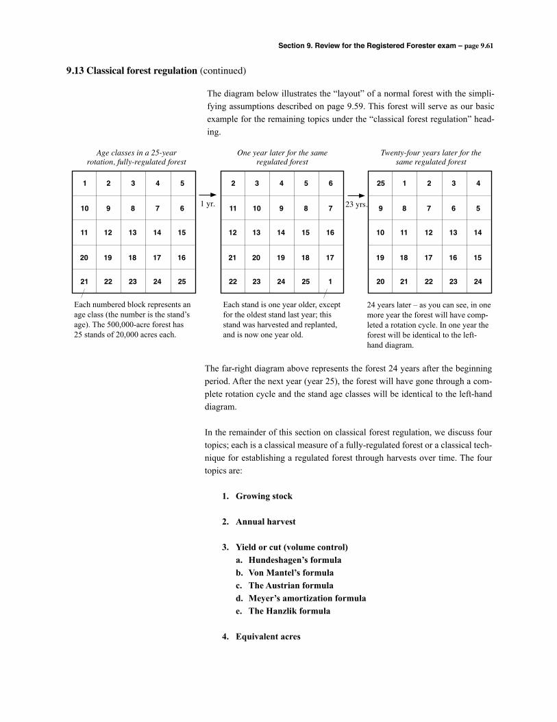
Section 9. Review for the Registered Forester exam – page 9.61
9.13 Classical forest regulation (continued)
The diagram below illustrates the “layout” of a normal forest with the simpli-fying assumptions described on page 9.59. This forest will serve as our basic example for the remaining topics under the “classical forest regulation” head-ing.
1 2 3 4 5
10 9 8 7 6
11 12 13 14 15
20 19 18 17 16
21 22 23 24 25
2 3 4 5 6
11 10 9 8 7
12 13 14 15 16
21 20 19 18 17
22 23 24 25 1
25 1 2 3 4
9 8 7 6 5
10 11 12 13 14
19 18 17 16 15
20 21 22 23 24
1 yr. 23 yrs.
Age classes in a 25-yearrotation, fully-regulated forest
One year later for the sameregulated forest
Twenty-four years later for thesame regulated forest
Each numbered block represents anage class (the number is the stand’sage). The 500,000-acre forest has 25 stands of 20,000 acres each.
Each stand is one year older, exceptfor the oldest stand last year; thisstand was harvested and replanted,and is now one year old.
24 years later – as you can see, in onemore year the forest will have comp-leted a rotation cycle. In one year theforest will be identical to the left-hand diagram.
The far-right diagram above represents the forest 24 years after the beginning period. After the next year (year 25), the forest will have gone through a com-plete rotation cycle and the stand age classes will be identical to the left-hand diagram.
In the remainder of this section on classical forest regulation, we discuss four topics; each is a classical measure of a fully-regulated forest or a classical tech-nique for establishing a regulated forest through harvests over time. The four topics are:
1. Growing stock
2. Annual harvest
3. Yield or cut (volume control) a. Hundeshagen’s formula b. Von Mantel’s formula c. The Austrian formula d. Meyer’s amortization formula e. The Hanzlik formula
4. Equivalent acres

Section 9. Review for the Registered Forester exam – page 9.62
9.13 Classical forest regulation (continued)
1. Growing stock
The total volume of growing stock, GS, is given by the summation of the volumes on each acre:
GS = aY1 + aY2 + aY3 + … + aYr–1 + aYr
= a ∑Y ii=1
r
where Yi is the yield per acre in age class i, and r is the rotation age.
Solved problem:60. The total volume of growing stock on the example forest is:
GS = aY1 + aY2 + aY3 + … + aY24 + aY25
= 20,000 (0) + 20,000 (0) + 20,000 (0) + … + 20,000 (63) + 20,000 (66)
= 20,000 ∑ Yi
= 20,000 (632) = 12,640,000 cords
i=1
r
Note that a yield table is often stated in 5-year or 10-year age classes. For example, consider the yield table below:
Age(years)
10
15
20
25
30
Yield(cords/ac.)
7
30
51
66
74
With this type of yield information, growing stock can be estimated using the summation formula. The summation formula is based on the assumption that yield for a stand is the yield table value for each yield table age class + one half the number of years between yield table ages. For example, the 10 year age and 7 cord per acre yield is assumed to translate to 7 cords per acre over the 7.5 to 12.5 year age class. The 25 year age and 66 cords per acre yield translates to 66 cords per acre over the 22.5 to 25 year age class (note that 25 is harvest age so yields at greater ages aren’t needed). The diagram on the next page illustrates this concept.
Four techniques forestablishing a fully-regulated forest over time … 1. Growing stock 2. Annual harvest 3. Volume control 4. Equivalent acres

Section 9. Review for the Registered Forester exam – page 9.63
9.13 Classical forest regulation (continued)
1. Growing stock (continued)
The summation formula is based on the assumption that yield for a stand is the yield table for each yield table age class + the number of years between yield table ages:
Four techniques forestablishing a fully-regulated forest over time …(continued)
5 10 15 20 25Stand Age (years)
70
60
50
40
30
20
10
Volume(cds./ac.)
Growing stock on the R = 25 stands …
Solved problem:61. In terms of the prior yield table and a 25-year rotation, growing stock on
25 acres is given by:
GS = 5(7 + 30 + 51 + 66/2) = 605 cords on 25 acres
There is an average of 24.2 cords per acre of growing stock (605⁄25 = 24.2). The growing stock on the entire forest is 12,100,000 cords, since 20,000 of the 25-acre blocks constitute the entire forest.
GS for the entire forest = 605 cds./ac. x 20,000 blocks = 12,100,000 cords
Note that the two estimates of growing stock differ (12,640,000 vs. 12,100,000). This is not unexpected. Both yield tables result in esti-mates, and the estimates will usually differ.
The summation formula is:
GS = n(Vn +V2n + V3n + … + Vr-n + )
Where n is the number of years between yield table entries,
Vi is the yield table volume at age i, and r is the rotation age.
Vr
2
Section 9. Review for the Registered Forester exam – page 9.64
9.13 Classical forest regulation (continued)
2. Annual harvest
The annual harvest from the forest (H) is the total yield from the oldest age class, or:
H = YR Where all variables are as previously defined, and R is the age of final harvest.
For our example forest, annual harvest is:
H = 20,000 (66) = 1,320,000 cords
Note that the sum of growth on an acre will equal the annual harvest; this means the annual harvest (H) will equal forest growth (G):
H = G = a YR
Note that mean annual increment (MAI) is defined as:
MAI = = = 2.64 cords/acre/year
If we multiply MAI by a/a:
MAI =
Recall that H = a YR and a R = A, so that:
MAI =
Or H = MAI x A
Solved problem:
61. For the forest example:
H = 6.64 x 500,000 = 1,320,000 cords
Four techniques forestablishing a fully-regulated forest over time … 1. Growing stock 2. Annual harvest 3. Volume control 4. Equivalent acres
66
25
YR
R
a YR
a R
H
A
Section 9. Review for the Registered Forester exam – page 9.65
9.13 Classical forest regulation (continued)
3. Yield or cut (volume control)
In the following discussion of volume control techniques for achieving a fully-regulated forest, we include:
a. Hundeshagen’s formula; b. Von Mantel’s formula; c. The Austrian formula; d. Meyer’s Amortization formula; and e. Hanzlik’s formula.
a. Hundeshagen’s formula This formula is an approximation technique to estimate growing stock
yield. It’s based on the assumption that a straight-line relationship exists between growing stock volume and yield. For example, this means that 90 percent of normal growing stock will produce 90 percent of a normal yield.
Hundeshagen’s formula is:
Solved problem: 63. For example, assume that a timber cruise of the 500,000-acre forest
discussed earlier determined actual growing stock of 10,112,000 cords (instead of the fully-regulated forest growing stock of 12,640,000 cords). Then actual yield is estimated as:
Four techniques forestablishing a fully-regulated forest over time … 1. Growing stock 2. Annual harvest 3. Volume control 4. Equivalent acres
Ya = GaYR
GR
Where Ya = actual yield,YR = yield of a fully-regulated forest,Ga = actual growing stock, andGR = growing stock in a fully- regulated forest.
Ya = 10,112,000
= 1,056,000 cords
1,320,000
12,640,000
Section 9. Review for the Registered Forester exam – page 9.66
9.13 Classical forest regulation (continued)
Four techniques forestablishing a fully-regulated forest over time … 1. Growing stock 2. Annual harvest 3. Volume control 4. Equivalent acres
GR = R YR
2
3. Yield or cut (volume control) (continued)
b. Von Mantel’s formula (also called the triangle formula) Von Mantel’s formula assumes that growing stock in a fully regulated
forest increases in a linear manner with age, which produces a right trian-gle relationship. Growing stock is represented by the area of the triangle. Recall the area of a right triangle is given by 1/2 x base x height (or in this case, 1/2 x R x YR). Then growing stock is:
Note that the estimate of actual yield we obtained with Von Mantel’s formula (808,960 cords) is considerably less than when we applied Hun-deshagen’s formula (1,056,000 cords). Von Mantel’s formula assumes that merchantable volume begins at year 0, while actually we know that merchantable volume doesn’t occur until years after a stand is regener-ated. In our example, merchantable volume begins at age 7 (or age 7.5 if the second yield table is used).
YR
R YR ÷ 2Ya = Ga
2 YR
R YR = Ga
2 Ga
R =
and if Hundeshagen’s formula is used to estimate actual yield, we obtain …
Solved problem:64. Using our same example and solving for actual yield using Von Man-
tel’s formula:
Ya = =2 Ga
R 2(10,112,000)
25
= 808,960 cords
Section 9. Review for the Registered Forester exam – page 9.67
9.13 Classical forest regulation (continued)
Four techniques forestablishing a fully-regulated forest over time … 1. Growing stock 2. Annual harvest 3. Volume control 4. Equivalent acres
3. Yield or cut (volume control) (continued)
b. Von Mantel’s formula (continued)
A modified Von Mantel’s formula assumes merchantable volume begins at the age of merchantability implied by the yield table. We still have a right triangle assumption in this case, but the area decreases.
c. The Austrian formula
The Austrian formula is a simple method to determine allowable cut. It assumes that the annual increment plus or minus the desired change in growing stock will produce the appropriate harvest quantity. The Austrian formula is:
Solved problem: 66. For example, assume that the present growing stock is 20 cords per
acre and the desired growing stock is 25 cords per acre. Annual incre-ment is 2.64 cords per acre and the adjustment period is 15 years:
Solved problem:65. Where am = age where merchantable volume first occurs, the modi-
fied Von Mantel’s formula is:
Ya = =2 Ga
R – am 2(10,112,000)
25 – 7
= 1,123,556 cords
Annual cut = I +Ga – GR
P
Where I = annual increment (usually periodic annual increment),
Ga = present growing stock, GR = desired growing stock, and P = adjustment period in years.
Annual cut = 2.64 +20 – 25
15
= 2.64 + (–0.33) = 2.31 cords
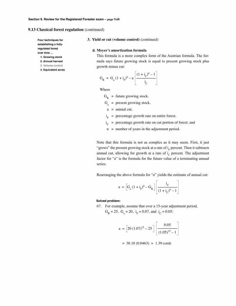
Section 9. Review for the Registered Forester exam – page 9.68
9.13 Classical forest regulation (continued)
Four techniques forestablishing a fully-regulated forest over time … 1. Growing stock 2. Annual harvest 3. Volume control 4. Equivalent acres
3. Yield or cut (volume control) (continued)
d. Meyer’s amortization formula This formula is a more complex form of the Austrian formula. The for-
mula says future growing stock is equal to present growing stock plus growth minus cut:
Note that this formula is not as complex as it may seem. First, it just “grows” the present growing stock at a rate of iF percent. Then it subtracts annual cut, allowing for growth at a rate of iC percent. The adjustment factor for “a” is the formula for the future value of a terminating annual series.
Rearranging the above formula for “a” yields the estimate of annual cut:
Solved problem: 67. For example, assume that over a 15-year adjustment period, GR = 25, Ga = 20, iF = 0.07, and iC = 0.05:
GR = Ga (1 + iF)n – a
Where
GR = future growing stock,
Ga = present growing stock,
a = annual cut,
iF = percentage growth rate on entire forest,
iC = percentage growth rate on cut portion of forest, and
n = number of years in the adjustment period.
(1 + iC)n – 1
iC
iC(1 + iC)n – 1
a = Ga (1 + iF)n – GR
a = 20 (1.07)15 – 250.05
(1.05)15 – 1
= 30.18 (0.0463) = 1.39 cords
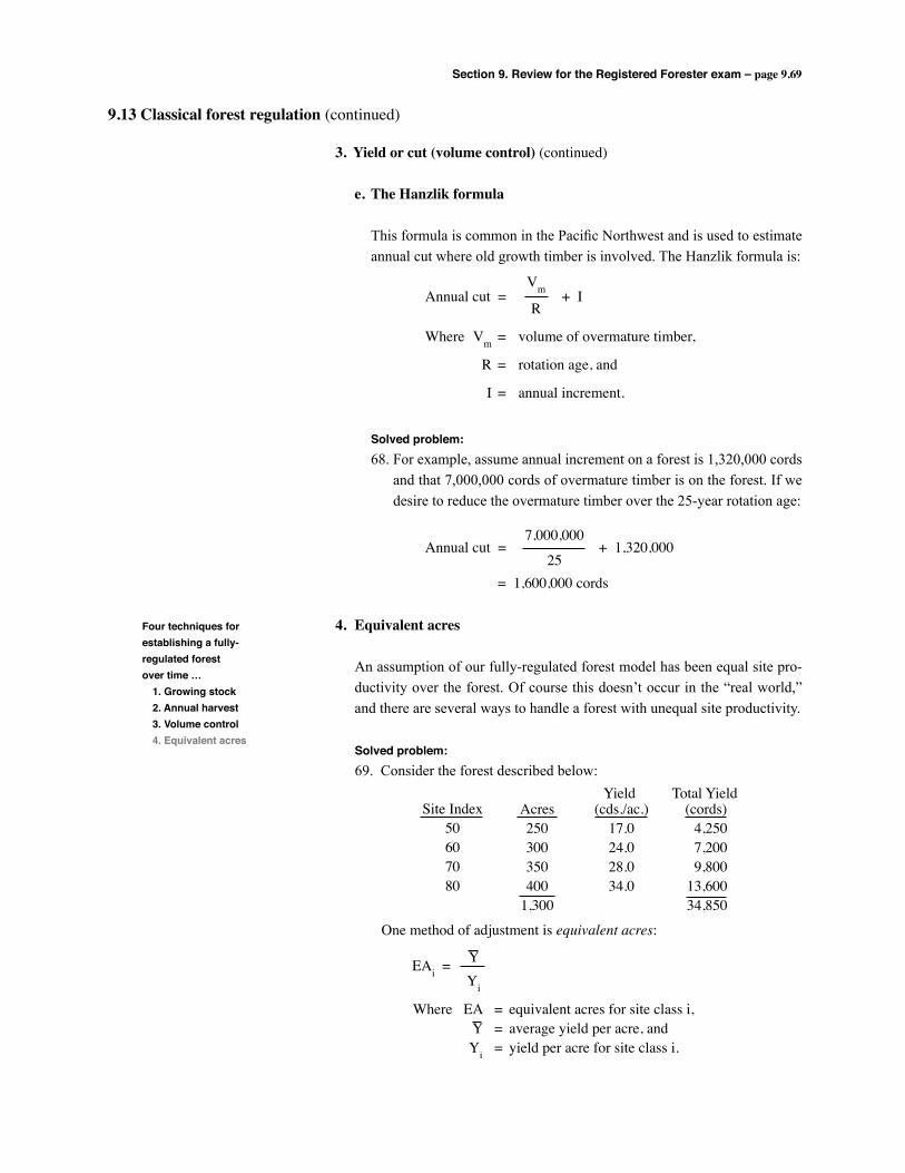
Section 9. Review for the Registered Forester exam – page 9.69
9.13 Classical forest regulation (continued)
Four techniques forestablishing a fully-regulated forest over time … 1. Growing stock 2. Annual harvest 3. Volume control 4. Equivalent acres
3. Yield or cut (volume control) (continued)
e. The Hanzlik formula
This formula is common in the Pacific Northwest and is used to estimate annual cut where old growth timber is involved. The Hanzlik formula is:
Solved problem: 68. For example, assume annual increment on a forest is 1,320,000 cords
and that 7,000,000 cords of overmature timber is on the forest. If we desire to reduce the overmature timber over the 25-year rotation age:
4. Equivalent acres
An assumption of our fully-regulated forest model has been equal site pro-ductivity over the forest. Of course this doesn’t occur in the “real world,” and there are several ways to handle a forest with unequal site productivity.
Annual cut = + I
Where Vm = volume of overmature timber,
R = rotation age, and
I = annual increment.
Vm
R
Annual cut = + 1,320,000
= 1,600,000 cords
7,000,000
25
Solved problem:69. Consider the forest described below:
Site Index50607080
Acres250300350400
1,300
(cds./ac.)17.024.028.034.0
(cords)4,2507,2009,800
13,60034,850
Yield Total Yield
One method of adjustment is equivalent acres:
EAi =YYi
Where EA = equivalent acres for site class i, Y = average yield per acre, and Yi = yield per acre for site class i.
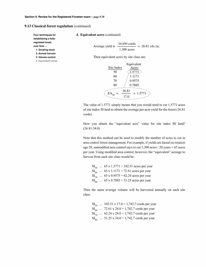
Section 9. Review for the Registered Forester exam – page 9.70
9.13 Classical forest regulation (continued)
Four techniques forestablishing a fully-regulated forest over time … 1. Growing stock 2. Annual harvest 3. Volume control 4. Equivalent acres
4. Equivalent acres (continued)
Average yield is = 26.81 cds./ac.34,850 cords
1,300 acres
Then equivalent acres by site class are:
Site Index50607080
Acres1.57711.11710.95750.7885
Equivalent
EA50 = = 1.5771 26.81
17.0
The value of 1.5771 simply means that you would need to cut 1.5771 acres of site index 50 land to obtain the average per-acre yield for the forest (26.81 cords).
How you obtain the “equivalent acre” value for site index 80 land? (26.81/34.0)
Note that this method can be used to modify the number of acres to cut in area control forest management. For example, if yields are based on rotation age 20, unmodified area control says to cut 1,300 acres / 20 years = 65 acres per year. Using modified area control, however, the “equivalent” acreage to harvest from each site class would be:
SI50 … 65 x 1.5771 = 102.51 acres per year SI60 … 65 x 1.1171 = 72.61 acres per year SI70 … 65 x 0.9575 = 62.24 acres per year SI80 … 65 x 0.7885 = 51.25 acres per year
Then the same average volume will be harvested annually on each site class:
SI50 … 102.51 x 17.0 = 1,742.7 cords per year SI60 … 72.61 x 24.0 = 1,742.7 cords per year SI70 … 62.24 x 28.0 = 1,742.7 cords per year SI80 … 51.25 x 34.0 = 1,742.7 cords per year
Section 9. Review for the Registered Forester exam – page 9.71
An overview of harvest scheduling …
“Harvest scheduling” can be done with mathematical programming techniques. These techniques schedule the harvests on a forest to maximize or minimize a specific objective. Examples of common objectives are:
• Maximize Net Present Value • Maximize Bare Land Value • Maximize Timber Production • Minimize Cost of Timber
Usually the objective is achieved subject to a set of constraints. Examples of common constraints are:
• Specified Revenue in Each Time Period • Specified Timber Flow Over Time • Specified Cash Flow Over Time • Specified Acreage Distribution Over Time
Linear programming (LP) includes a class of mathematical programming tech-niques originally developed in the field of operations research. LP methods are widely applied in forest management. Use of LP requires a linear objective function and linear constraints. To solve a harvest scheduling problem using LP, the problem is usually simplified to avoid unnecessary complexity.
General steps in applying LP to the timber harvest scheduling problem are:
• Determine the planning horizon and the length of the cutting period. The planning horizon is the time period over which harvests will be scheduled. This limits the size of the problem. Two rotation lengths is a common planning horizon (50-60 years in the South).
• Determine the cutting units. What area on the forest is to be scheduled for harvest? This might be stands or age classes.
• Determine the relevant management regimes. A management regime is the schedule of planned activities on a particular cutting unit. For exam-ple, site prepare at year 1, plant at year 2, thin at year 17, and clearcut at year 25.
9.14 Linear programming – area and volume control
We present a brief overview of harvest scheduling, and a brief review of area control and volume control in the context of a linear program-ming harvest scheduling problem.
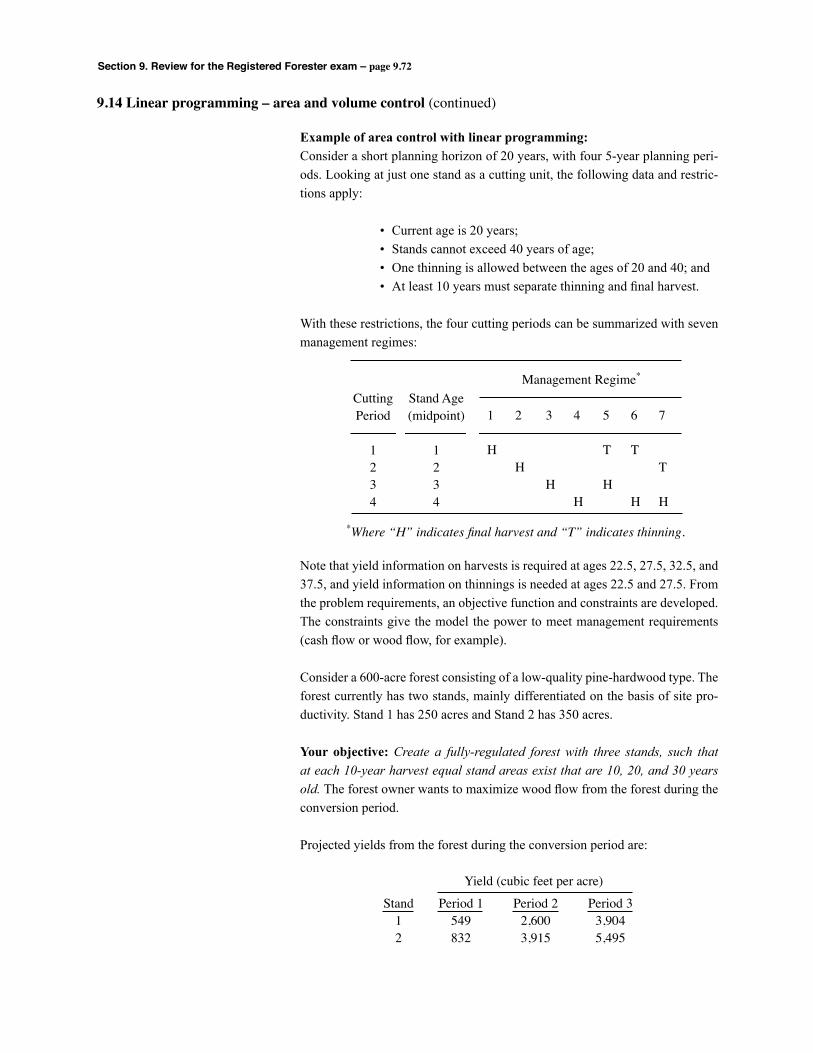
Section 9. Review for the Registered Forester exam – page 9.72
9.14 Linear programming – area and volume control (continued)
Example of area control with linear programming:Consider a short planning horizon of 20 years, with four 5-year planning peri-ods. Looking at just one stand as a cutting unit, the following data and restric-tions apply:
• Current age is 20 years; • Stands cannot exceed 40 years of age; • One thinning is allowed between the ages of 20 and 40; and • At least 10 years must separate thinning and final harvest.
With these restrictions, the four cutting periods can be summarized with seven management regimes:
Note that yield information on harvests is required at ages 22.5, 27.5, 32.5, and 37.5, and yield information on thinnings is needed at ages 22.5 and 27.5. From the problem requirements, an objective function and constraints are developed. The constraints give the model the power to meet management requirements (cash flow or wood flow, for example).
Consider a 600-acre forest consisting of a low-quality pine-hardwood type. The forest currently has two stands, mainly differentiated on the basis of site pro-ductivity. Stand 1 has 250 acres and Stand 2 has 350 acres.
Your objective: Create a fully-regulated forest with three stands, such that at each 10-year harvest equal stand areas exist that are 10, 20, and 30 years old. The forest owner wants to maximize wood flow from the forest during the conversion period.
Projected yields from the forest during the conversion period are:
1 2 3 4 5 6 7
H T T H T H H H H H
Management Regime*
CuttingPeriod
1234
Stand Age(midpoint)
1234
*Where “H” indicates final harvest and “T” indicates thinning.
Period 1549832
Period 22,6003,915
Period 33,9045,495
Stand12
Yield (cubic feet per acre)
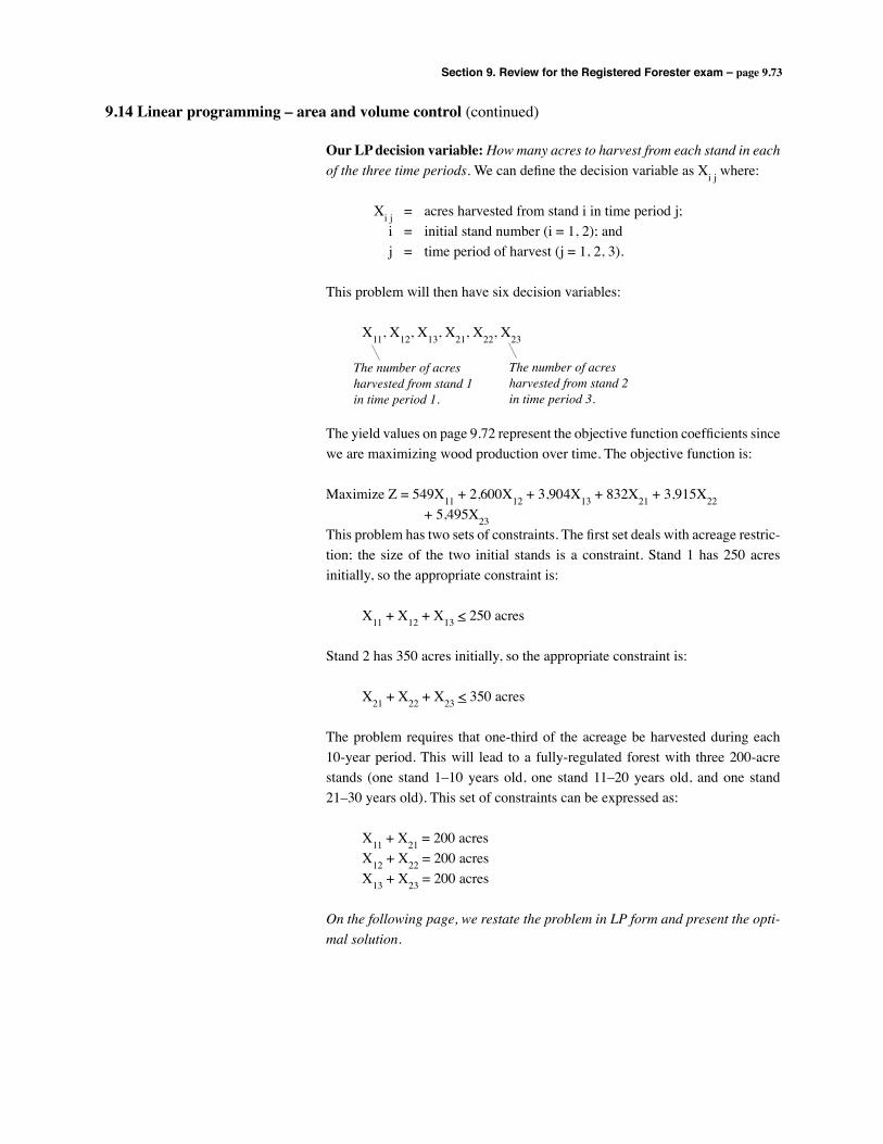
Section 9. Review for the Registered Forester exam – page 9.73
9.14 Linear programming – area and volume control (continued)
Our LP decision variable: How many acres to harvest from each stand in each of the three time periods. We can define the decision variable as Xi j where:
Xi j = acres harvested from stand i in time period j; i = initial stand number (i = 1, 2); and j = time period of harvest (j = 1, 2, 3).
This problem will then have six decision variables:
X11, X12, X13, X21, X22, X23
The yield values on page 9.72 represent the objective function coefficients since we are maximizing wood production over time. The objective function is:
Maximize Z = 549X11 + 2,600X12 + 3,904X13 + 832X21 + 3,915X22 + 5,495X23This problem has two sets of constraints. The first set deals with acreage restric-tion; the size of the two initial stands is a constraint. Stand 1 has 250 acres initially, so the appropriate constraint is:
X11 + X12 + X13 < 250 acres
Stand 2 has 350 acres initially, so the appropriate constraint is:
X21 + X22 + X23 < 350 acres
The problem requires that one-third of the acreage be harvested during each 10-year period. This will lead to a fully-regulated forest with three 200-acre stands (one stand 1–10 years old, one stand 11–20 years old, and one stand 21–30 years old). This set of constraints can be expressed as:
X11 + X21 = 200 acres X12 + X22 = 200 acres X13 + X23 = 200 acres
On the following page, we restate the problem in LP form and present the opti-mal solution.
The number of acresharvested from stand 1 in time period 1.
The number of acresharvested from stand 2 in time period 3.

Section 9. Review for the Registered Forester exam – page 9.74
9.14 Linear programming – area and volume control (continued)
The entire problem on page 9.73 can be formulated as:
Maximize Z = 549X11 + 2,600X12 + 3,904X13 + 832 X21 + 3,915X22 + 5,495X23
Subject to: X11 + X12 + X13 < 250 acres X21 + X22 + X23 < 350 acres X11 + X21 = 200 acres X12 + X22 = 200 acres X13 + X23 = 200 acres Xi j > 0 for all i and j
The optimal solution is:
Z* = 1,926,000 cubic feet X11 = 200 acres X12 = 50 acres X13 = 0 acres X21 = 0 acres X22 = 150 acres X23 = 200 acres
The harvest volume for each time period is presented below:
Period 1109,800
0109,800
Period 2130,000587,250717,250
Period 30
1,099,0001,099,000
Stand12
Harvest Volume (cubic feet)
Total239,800
1,686,2501,926,050
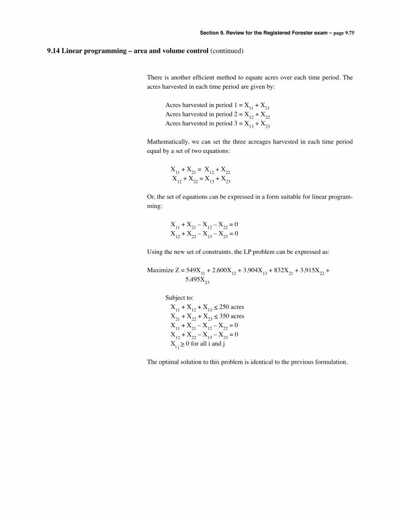
Section 9. Review for the Registered Forester exam – page 9.75
9.14 Linear programming – area and volume control (continued)
There is another efficient method to equate acres over each time period. The acres harvested in each time period are given by:
Acres harvested in period 1 = X11 + X21 Acres harvested in period 2 = X12 + X22 Acres harvested in period 3 = X13 + X23
Mathematically, we can set the three acreages harvested in each time period equal by a set of two equations:
X11 + X21 = X12 + X22 X12 + X22 = X13 + X23
Or, the set of equations can be expressed in a form suitable for linear program-ming:
X11 + X21 – X12 – X22 = 0 X12 + X22 – X13 – X23 = 0
Using the new set of constraints, the LP problem can be expressed as:
Maximize Z = 549X11 + 2,600X12 + 3,904X13 + 832X21 + 3,915X22 + 5,495X23
Subject to: X11 + X12 + X13 < 250 acres X21 + X22 + X23 < 350 acres X11 + X21 – X12 – X22 = 0 X12 + X22 – X13 – X23 = 0 Xi j > 0 for all i and j
The optimal solution to this problem is identical to the previous formulation.
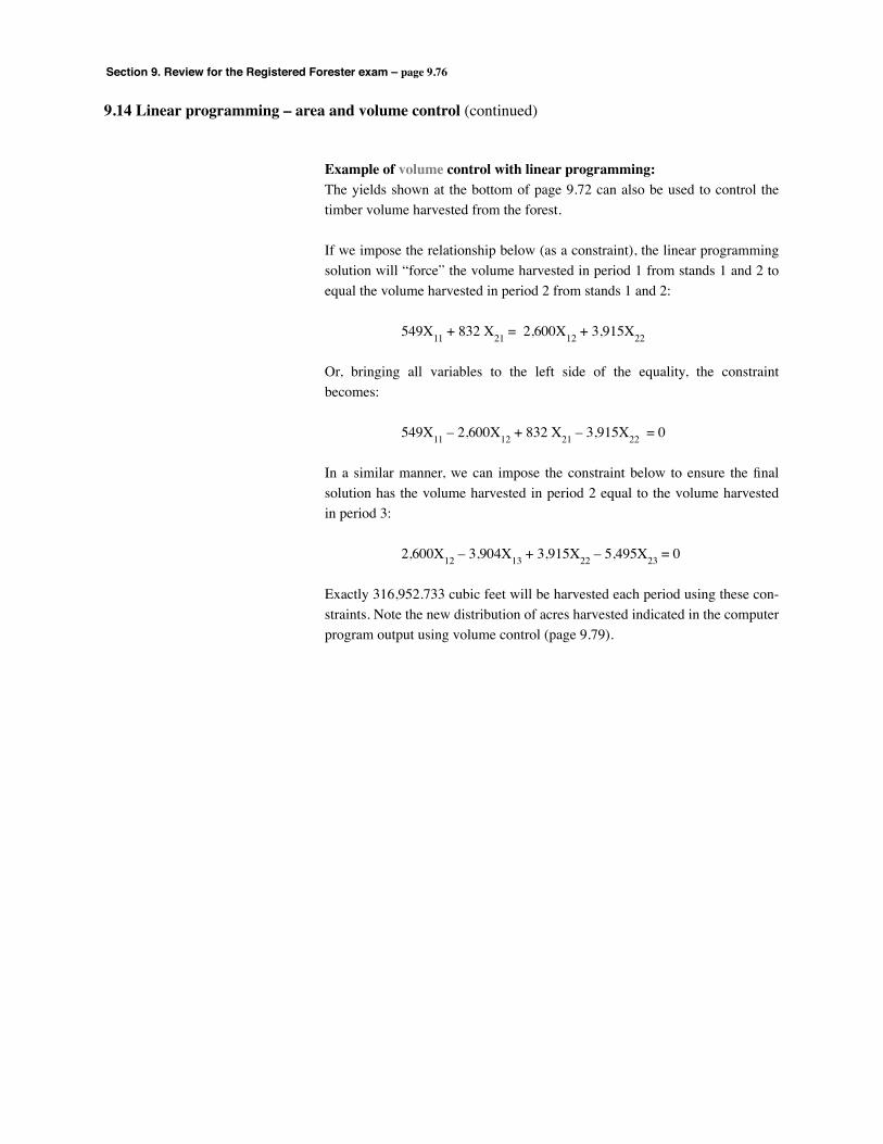
Section 9. Review for the Registered Forester exam – page 9.76
9.14 Linear programming – area and volume control (continued)
Example of volume control with linear programming:The yields shown at the bottom of page 9.72 can also be used to control the timber volume harvested from the forest.
If we impose the relationship below (as a constraint), the linear programming solution will “force” the volume harvested in period 1 from stands 1 and 2 to equal the volume harvested in period 2 from stands 1 and 2:
549X11 + 832 X21 = 2,600X12 + 3,915X22
Or, bringing all variables to the left side of the equality, the constraint becomes:
549X11 – 2,600X12 + 832 X21 – 3,915X22 = 0
In a similar manner, we can impose the constraint below to ensure the final solution has the volume harvested in period 2 equal to the volume harvested in period 3:
2,600X12 – 3,904X13 + 3,915X22 – 5,495X23 = 0
Exactly 316,952.733 cubic feet will be harvested each period using these con-straints. Note the new distribution of acres harvested indicated in the computer program output using volume control (page 9.79).
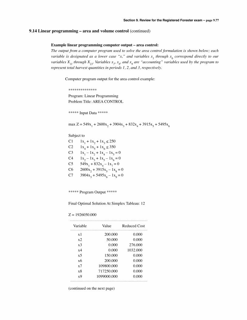
Section 9. Review for the Registered Forester exam – page 9.77
9.14 Linear programming – area and volume control (continued)
Example linear programming computer output – area control:The output from a computer program used to solve the area control formulation is shown below; each variable is designated as a lower case “x,” and variables x1 through x6 correspond directly to our variables X11 through X23. Variables x7, x8, and x9 are “accounting” variables used by the program to represent total harvest quantities in periods 1, 2, and 3, respectively.
Computer program output for the area control example:
************** Program: Linear Programming Problem Title: AREA CONTROL ***** Input Data *****
max Z = 549x1 + 2600x2 + 3904x3 + 832x4 + 3915x5 + 5495x6
Subject to C1 1x1 + 1x2 + 1x3 < 250 C2 1x4 + 1x5 + 1x6 < 350 C3 1x1 – 1x2 + 1x4 – 1x5 = 0 C4 1x2 – 1x3 + 1x5 – 1x6 = 0 C5 549x1 + 832x4 – 1x7 = 0 C6 2600x2 + 3915x5 – 1x8 = 0 C7 3904x3 + 5495x6 – 1x9 = 0
***** Program Output *****
Final Optimal Solution At Simplex Tableau: 12
Z = 1926050.000
(continued on the next page)
Variable
x1x2x3x4x5x6x7x8x9
Value
200.00050.0000.0000.000
150.000200.000
109800.000717250.000
1099000.000
Reduced Cost
0.0000.000
276.0001032.000
0.0000.0000.0000.0000.000

Section 9. Review for the Registered Forester exam – page 9.78
9.14 Linear programming – area and volume control (continued)
Example linear programming control output – area control:
(continued from the previous page) …
Variable
x1x2x3x4x5x6x7x8x9
Limit
-483.0002324.000No limitNo limit
2883.0005219.000No limit
-0.785-0.173
Current Values
549.0002600.0003904.000832.000
3915.0005495.000
0.0000.0000.000
Lower Limit
No limit3632.0004180.0001864.0004191.000No limit
3.6470.210
No limit
Upper Increase
No limit1032.000276.000
1032.000276.000No limit
3.6470.210
No limit
Allowable Decrease
1032.000276.000No limitNo limit
1032.000276.000No limit
0.7850.173
Allowable
Objective Coefficient Ranges
Constraints
C1C2C3C4C5C6C7
Limit
175.000125.000
-300.000-225.000No limitNo limitNo limit
Current Values
250.000350.000
3904.0000.0000.0000.0000.000
Lower Limit
700.000500.00075.000
150.000109800.000717250.000
1099000.000
Upper Increase
450.000150.00075.000
150.000109800.000717250.000
1099000.000
Allowable Decrease
75.000225.000300.000225.000No limitNo limitNo limit
Allowable
Right Hand Side Ranges
***** End of Output *****
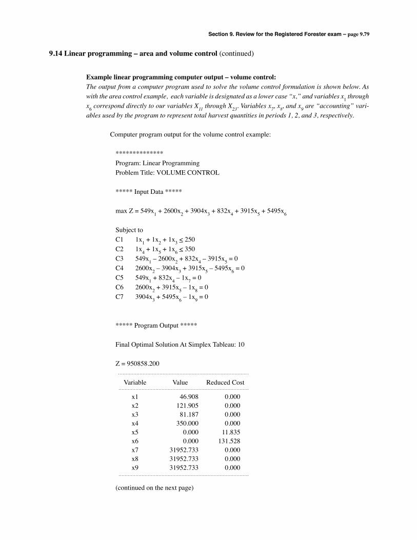
Section 9. Review for the Registered Forester exam – page 9.79
9.14 Linear programming – area and volume control (continued)
Example linear programming computer output – volume control:The output from a computer program used to solve the volume control formulation is shown below. As with the area control example, each variable is designated as a lower case “x,” and variables x1 through x6 correspond directly to our variables X11 through X23. Variables x7, x8, and x9 are “accounting” vari-ables used by the program to represent total harvest quantities in periods 1, 2, and 3, respectively.
Computer program output for the volume control example:
************** Program: Linear Programming Problem Title: VOLUME CONTROL ***** Input Data *****
max Z = 549x1 + 2600x2 + 3904x3 + 832x4 + 3915x5 + 5495x6
Subject to C1 1x1 + 1x2 + 1x3 < 250 C2 1x4 + 1x5 + 1x6 < 350 C3 549x1 – 2600x2 + 832x4 – 3915x5 = 0 C4 2600x2 – 3904x3 + 3915x5 – 5495x6 = 0 C5 549x1 + 832x4 – 1x7 = 0 C6 2600x2 + 3915x5 – 1x8 = 0 C7 3904x3 + 5495x6 – 1x9 = 0
***** Program Output *****
Final Optimal Solution At Simplex Tableau: 10
Z = 950858.200
(continued on the next page)
Variable
x1x2x3x4x5x6x7x8x9
Value
46.908121.90581.187
350.0000.0000.000
31952.73331952.73331952.733
Reduced Cost
0.0000.0000.0000.000
11.835131.528
0.0000.0000.000
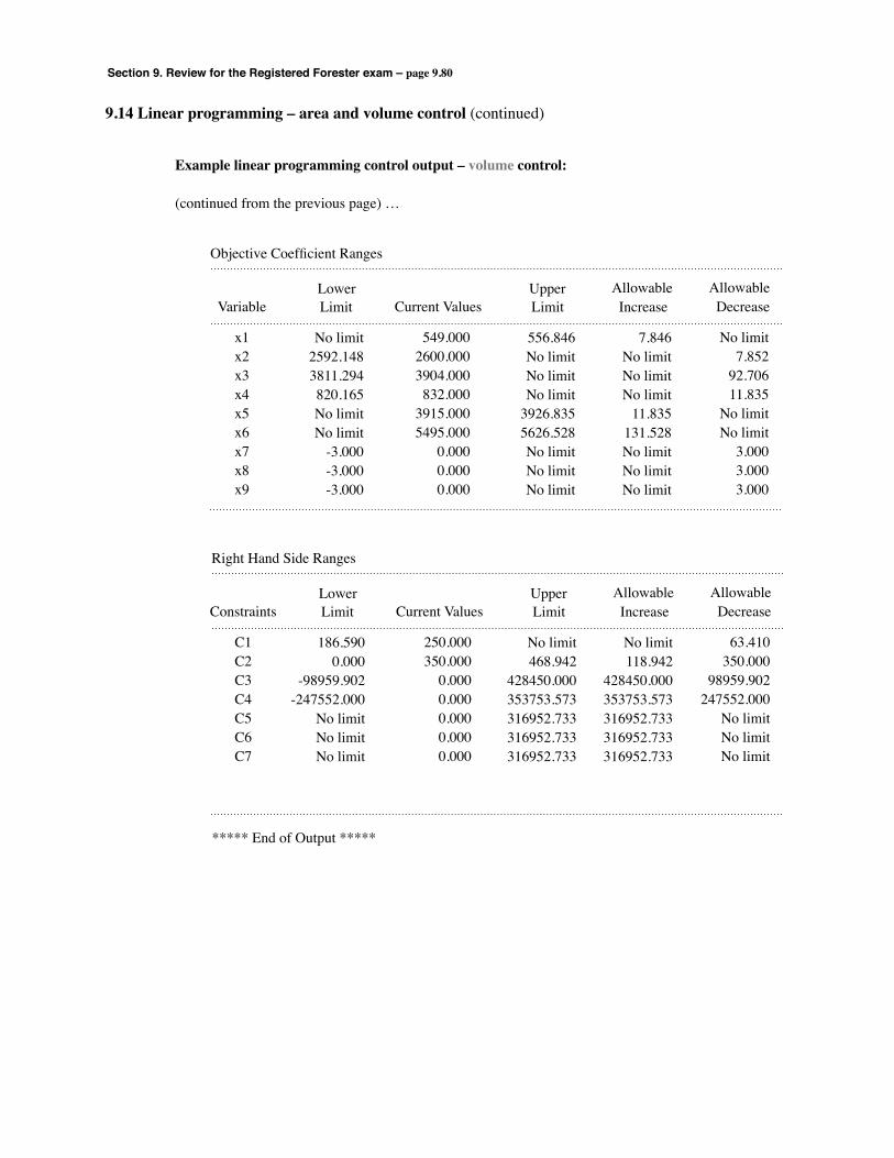
Section 9. Review for the Registered Forester exam – page 9.80
9.14 Linear programming – area and volume control (continued)
Example linear programming control output – volume control:
(continued from the previous page) …
Variable
x1x2x3x4x5x6x7x8x9
Limit
No limit2592.1483811.294820.165No limitNo limit
-3.000-3.000-3.000
Current Values
549.0002600.0003904.000832.000
3915.0005495.000
0.0000.0000.000
Lower Limit
556.846No limitNo limitNo limit
3926.8355626.528No limitNo limitNo limit
Upper Increase
7.846No limitNo limitNo limit
11.835131.528No limitNo limitNo limit
Allowable Decrease
No limit7.852
92.70611.835
No limitNo limit
3.0003.0003.000
Allowable
Objective Coefficient Ranges
Constraints
C1C2C3C4C5C6C7
Limit
186.5900.000
-98959.902-247552.000
No limitNo limitNo limit
Current Values
250.000350.000
0.0000.0000.0000.0000.000
Lower Limit
No limit468.942
428450.000353753.573316952.733316952.733316952.733
Upper Increase
No limit118.942
428450.000353753.573316952.733316952.733316952.733
Allowable Decrease
63.410350.000
98959.902247552.000
No limitNo limitNo limit
Allowable
Right Hand Side Ranges
***** End of Output *****
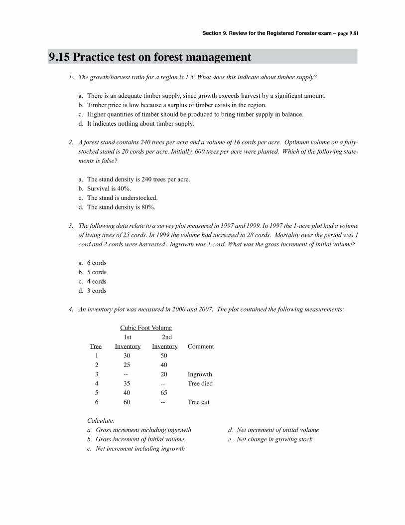
Section 9. Review for the Registered Forester exam – page 9.81
9.15 Practice test on forest management1. The growth/harvest ratio for a region is 1.5. What does this indicate about timber supply?
a. There is an adequate timber supply, since growth exceeds harvest by a significant amount. b. Timber price is low because a surplus of timber exists in the region. c. Higher quantities of timber should be produced to bring timber supply in balance. d. It indicates nothing about timber supply.
2. A forest stand contains 240 trees per acre and a volume of 16 cords per acre. Optimum volume on a fully-stocked stand is 20 cords per acre. Initially, 600 trees per acre were planted. Which of the following state-ments is false?
a. The stand density is 240 trees per acre. b. Survival is 40%. c. The stand is understocked. d. The stand density is 80%.
3. The following data relate to a survey plot measured in 1997 and 1999. In 1997 the 1-acre plot had a volume of living trees of 25 cords. In 1999 the volume had increased to 28 cords. Mortality over the period was 1 cord and 2 cords were harvested. Ingrowth was 1 cord. What was the gross increment of initial volume?
a. 6 cords b. 5 cords c. 4 cords d. 3 cords
4. An inventory plot was measured in 2000 and 2007. The plot contained the following measurements:
Cubic Foot Volume 1st 2nd Tree Inventory Inventory Comment 1 30 50 2 25 40 3 -- 20 Ingrowth 4 35 -- Tree died 5 40 65 6 60 -- Tree cut
Calculate: a. Gross increment including ingrowth d. Net increment of initial volume b. Gross increment of initial volume e. Net change in growing stock c. Net increment including ingrowth
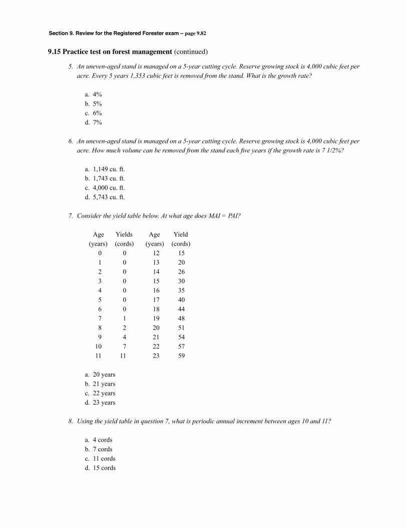
Section 9. Review for the Registered Forester exam – page 9.82
9.15 Practice test on forest management (continued)
5. An uneven-aged stand is managed on a 5-year cutting cycle. Reserve growing stock is 4,000 cubic feet per acre. Every 5 years 1,353 cubic feet is removed from the stand. What is the growth rate?
a. 4% b. 5% c. 6% d. 7%
6. An uneven-aged stand is managed on a 5-year cutting cycle. Reserve growing stock is 4,000 cubic feet per acre. How much volume can be removed from the stand each five years if the growth rate is 7 1/2%?
a. 1,149 cu. ft. b. 1,743 cu. ft. c. 4,000 cu. ft. d. 5,743 cu. ft.
7. Consider the yield table below. At what age does MAI = PAI?
Age Yields Age Yield (years) (cords) (years) (cords) 0 0 12 15 1 0 13 20 2 0 14 26 3 0 15 30 4 0 16 35 5 0 17 40 6 0 18 44 7 1 19 48 8 2 20 51 9 4 21 54 10 7 22 57 11 11 23 59
a. 20 years b. 21 years c. 22 years d. 23 years
8. Using the yield table in question 7, what is periodic annual increment between ages 10 and 11?
a. 4 cords b. 7 cords c. 11 cords d. 15 cords
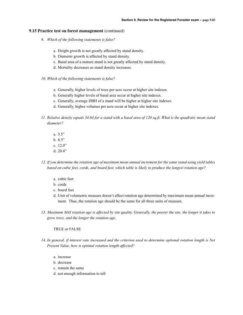
Section 9. Review for the Registered Forester exam – page 9.83
9.15 Practice test on forest management (continued)
9. Which of the following statements is false?
a. Height growth is not greatly affected by stand density. b. Diameter growth is affected by stand density. c. Basal area of a mature stand is not greatly affected by stand density. d. Mortality decreases as stand density increases.
10. Which of the following statements is false?
a. Generally, higher levels of trees per acre occur at higher site indexes. b. Generally higher levels of basal area occur at higher site indexes. c. Generally, average DBH of a stand will be higher at higher site indexes. d. Generally, higher volumes per acre occur at higher site indexes.
11. Relative density equals 34.64 for a stand with a basal area of 120 sq.ft. What is the quadratic mean stand diameter?
a. 3.5” b. 8.5” c. 12.0” d. 20.4”
12. If you determine the rotation age of maximum mean annual increment for the same stand using yield tables based on cubic feet, cords, and board feet, which table is likely to produce the longest rotation age?
a. cubic feet b. cords c. board feet d. Unit of volumetric measure doesn’t affect rotation age determined by maximum mean annual incre-
ment. Thus, the rotation age should be the same for all three units of measure.
13. Maximum MAI rotation age is affected by site quality. Generally, the poorer the site, the longer it takes to grow trees, and the longer the rotation age.
TRUE or FALSE
14. In general, if interest rate increased and the criterion used to determine optional rotation length is Net Present Value, how is optimal rotation length affected?
a. increase b. decrease c. remain the same d. not enough information to tell

Section 9. Review for the Registered Forester exam – page 9.84
9.15 Practice test on forest management (continued)
15. Using the yield table below, what is the rotation age that maximizes Internal Rate of Return? Use the cost and price data below to solve the problem.
Year* Item Amount 0 Regeneration -$120.00 R Harvest +104/cu. ft. 1-R Annual Mgmt. Cost -$2.50/ac 1-R Annual Hunting Lease Revenue +$2.50/ac *R = rotation age Age Yield (years) (cubic feet) 5 100 10 700 15 3,000 20 5,000 25 6,500 30 7,800
a. 15 years b. 20 years c. 25 years d. 30 years
16. Assume you measure all the trees on a 1-acre plot. Below is the stand table. What are the basal area, stand density index, and relative spacing? Average height of dominants is 60 feet (assume square spacing).
Trees Per DBH Acre 6 31 8 23 10 24 12 12 14 8 16 6 18 5 109
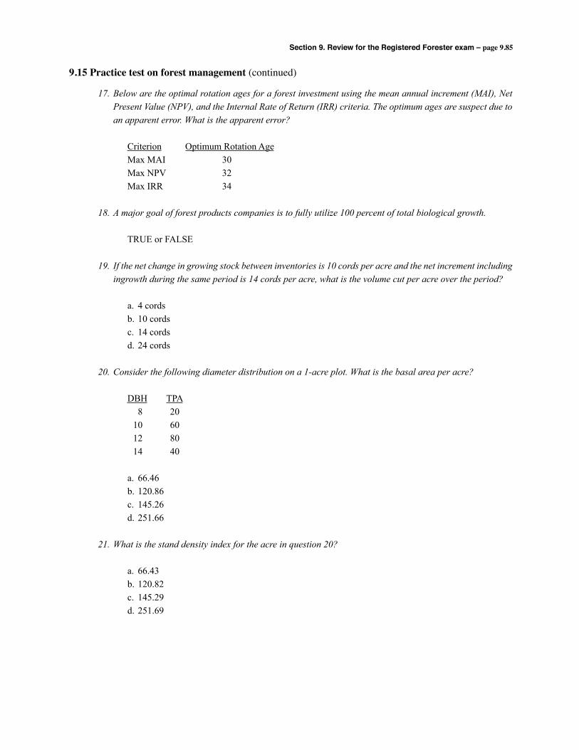
Section 9. Review for the Registered Forester exam – page 9.85
9.15 Practice test on forest management (continued)
17. Below are the optimal rotation ages for a forest investment using the mean annual increment (MAI), Net Present Value (NPV), and the Internal Rate of Return (IRR) criteria. The optimum ages are suspect due to an apparent error. What is the apparent error?
Criterion Optimum Rotation Age Max MAI 30 Max NPV 32 Max IRR 34
18. A major goal of forest products companies is to fully utilize 100 percent of total biological growth.
TRUE or FALSE
19. If the net change in growing stock between inventories is 10 cords per acre and the net increment including ingrowth during the same period is 14 cords per acre, what is the volume cut per acre over the period?
a. 4 cords b. 10 cords c. 14 cords d. 24 cords
20. Consider the following diameter distribution on a 1-acre plot. What is the basal area per acre?
DBH TPA 8 20 10 60 12 80 14 40
a. 66.46 b. 120.86 c. 145.26 d. 251.66
21. What is the stand density index for the acre in question 20?
a. 66.43 b. 120.82 c. 145.29 d. 251.69
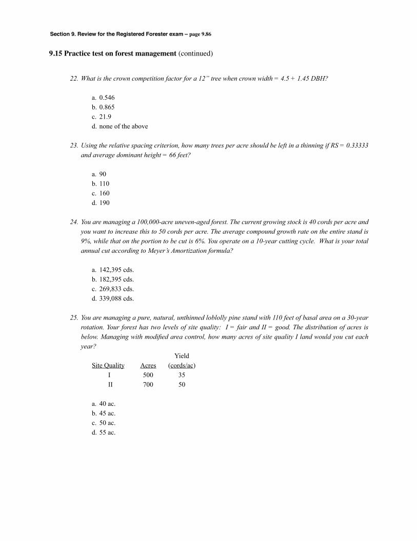
Section 9. Review for the Registered Forester exam – page 9.86
9.15 Practice test on forest management (continued)
22. What is the crown competition factor for a 12” tree when crown width = 4.5 + 1.45 DBH?
a. 0.546 b. 0.865 c. 21.9 d. none of the above
23. Using the relative spacing criterion, how many trees per acre should be left in a thinning if RS = 0.33333 and average dominant height = 66 feet?
a. 90 b. 110 c. 160 d. 190
24. You are managing a 100,000-acre uneven-aged forest. The current growing stock is 40 cords per acre and you want to increase this to 50 cords per acre. The average compound growth rate on the entire stand is 9%, while that on the portion to be cut is 6%. You operate on a 10-year cutting cycle. What is your total annual cut according to Meyer’s Amortization formula?
a. 142,395 cds. b. 182,395 cds. c. 269,833 cds. d. 339,088 cds.
25. You are managing a pure, natural, unthinned loblolly pine stand with 110 feet of basal area on a 30-year rotation. Your forest has two levels of site quality: I = fair and II = good. The distribution of acres is below. Managing with modified area control, how many acres of site quality I land would you cut each year?
Yield Site Quality Acres (cords/ac) I 500 35 II 700 50
a. 40 ac. b. 45 ac. c. 50 ac. d. 55 ac.
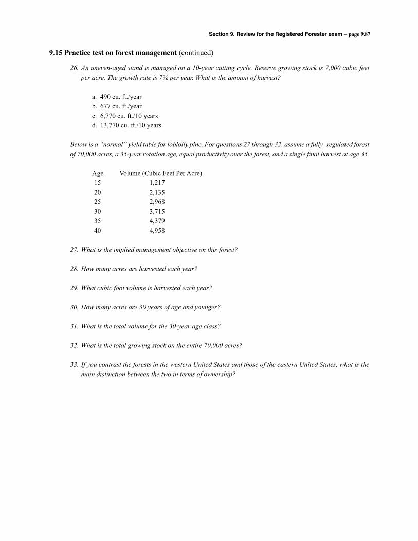
Section 9. Review for the Registered Forester exam – page 9.87
9.15 Practice test on forest management (continued)
26. An uneven-aged stand is managed on a 10-year cutting cycle. Reserve growing stock is 7,000 cubic feet per acre. The growth rate is 7% per year. What is the amount of harvest?
a. 490 cu. ft./year b. 677 cu. ft./year c. 6,770 cu. ft./10 years d. 13,770 cu. ft./10 years
Below is a “normal” yield table for loblolly pine. For questions 27 through 32, assume a fully- regulated forest of 70,000 acres, a 35-year rotation age, equal productivity over the forest, and a single final harvest at age 35.
Age Volume (Cubic Feet Per Acre) 15 1,217 20 2,135 25 2,968 30 3,715 35 4,379 40 4,958
27. What is the implied management objective on this forest?
28. How many acres are harvested each year?
29. What cubic foot volume is harvested each year?
30. How many acres are 30 years of age and younger?
31. What is the total volume for the 30-year age class?
32. What is the total growing stock on the entire 70,000 acres?
33. If you contrast the forests in the western United States and those of the eastern United States, what is the main distinction between the two in terms of ownership?
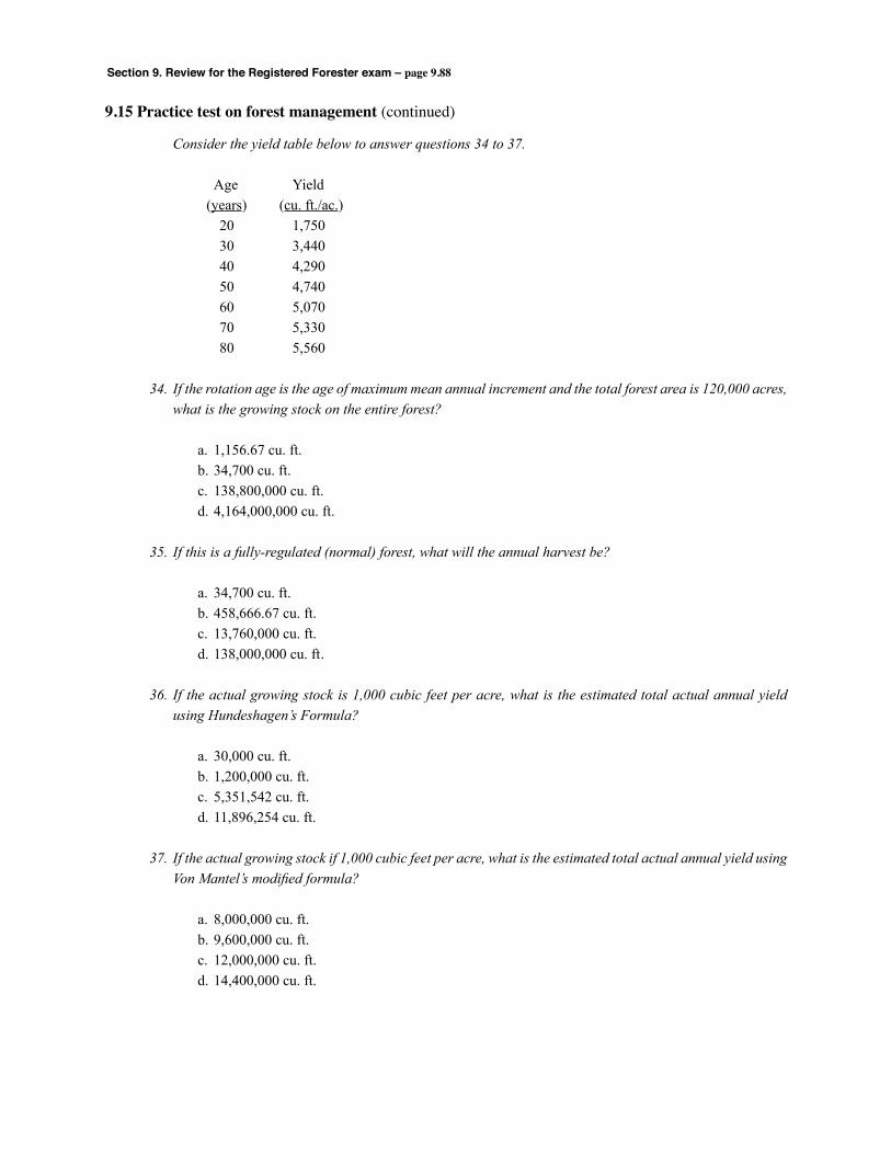
Section 9. Review for the Registered Forester exam – page 9.88
9.15 Practice test on forest management (continued)
Consider the yield table below to answer questions 34 to 37.
Age Yield (years) (cu. ft./ac.) 20 1,750 30 3,440 40 4,290 50 4,740 60 5,070 70 5,330 80 5,560
34. If the rotation age is the age of maximum mean annual increment and the total forest area is 120,000 acres, what is the growing stock on the entire forest?
a. 1,156.67 cu. ft. b. 34,700 cu. ft. c. 138,800,000 cu. ft. d. 4,164,000,000 cu. ft.
35. If this is a fully-regulated (normal) forest, what will the annual harvest be?
a. 34,700 cu. ft. b. 458,666.67 cu. ft. c. 13,760,000 cu. ft. d. 138,000,000 cu. ft.
36. If the actual growing stock is 1,000 cubic feet per acre, what is the estimated total actual annual yield using Hundeshagen’s Formula?
a. 30,000 cu. ft. b. 1,200,000 cu. ft. c. 5,351,542 cu. ft. d. 11,896,254 cu. ft.
37. If the actual growing stock if 1,000 cubic feet per acre, what is the estimated total actual annual yield using Von Mantel’s modified formula?
a. 8,000,000 cu. ft. b. 9,600,000 cu. ft. c. 12,000,000 cu. ft. d. 14,400,000 cu. ft.

Section 9. Review for the Registered Forester exam – page 9.89
9.15 Practice test on forest management (continued)
Below is a yield table for loblolly pine, site index 70 (base age 25), 9 x 10 spacing. Assume a fully-regulated (normal) forest with a rotation age of 22 years. Use this table to answer questions 38 to 41.
Age Yield Age Yield (years) (cords) (years) (cords) 0 0 12 15 1 0 13 20 2 0 14 26 3 0 15 30 4 0 16 35 5 0 17 40 6 0 18 44 7 1 19 48 8 2 20 51 9 4 21 54 10 7 22 57 11 11 23 59
38. If total forest area is 440,000 acres, how many acres are in each age class?
a. 20,000 acres b. 24,667 acres c. 44,000 acres d. 44,667 acres
39. What is the total growing stock on the entire forest?
a. 445,000 cords b. 4,450,000 cords c. 6,200,000 cords d. 8,900,000 cords
40. What is the annual harvest from this fully-regulated forest?
a. 1,140,000 cords b. 1,640,000 cords c. 1,864,000 cords d. 2,200,000 cords
41. How many acres of the forest contain trees 15 years of age and younger?
a. 150,000 acres b. 270,000 acres c. 300,000 acres d. 4,125,000 acres
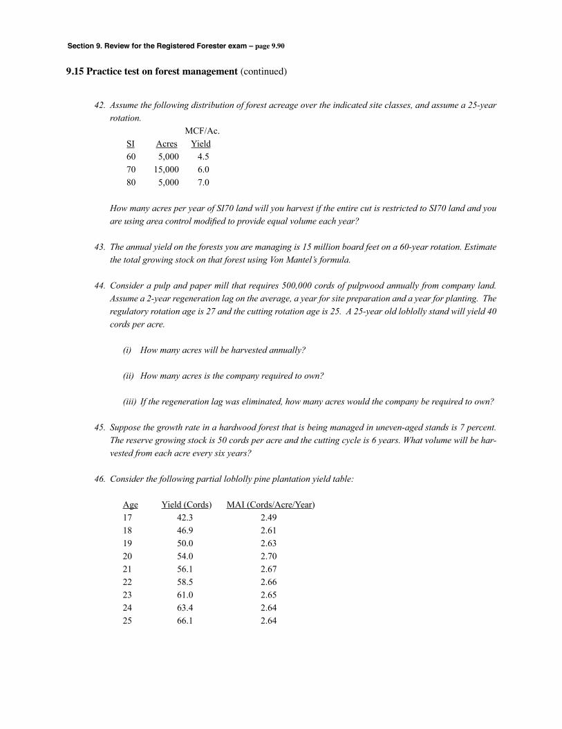
Section 9. Review for the Registered Forester exam – page 9.90
9.15 Practice test on forest management (continued)
42. Assume the following distribution of forest acreage over the indicated site classes, and assume a 25-year rotation.
MCF/Ac. SI Acres Yield 60 5,000 4.5 70 15,000 6.0 80 5,000 7.0
How many acres per year of SI70 land will you harvest if the entire cut is restricted to SI70 land and you are using area control modified to provide equal volume each year?
43. The annual yield on the forests you are managing is 15 million board feet on a 60-year rotation. Estimate the total growing stock on that forest using Von Mantel’s formula.
44. Consider a pulp and paper mill that requires 500,000 cords of pulpwood annually from company land. Assume a 2-year regeneration lag on the average, a year for site preparation and a year for planting. The regulatory rotation age is 27 and the cutting rotation age is 25. A 25-year old loblolly stand will yield 40 cords per acre.
(i) How many acres will be harvested annually?
(ii) How many acres is the company required to own?
(iii) If the regeneration lag was eliminated, how many acres would the company be required to own?
45. Suppose the growth rate in a hardwood forest that is being managed in uneven-aged stands is 7 percent. The reserve growing stock is 50 cords per acre and the cutting cycle is 6 years. What volume will be har-vested from each acre every six years?
46. Consider the following partial loblolly pine plantation yield table:
Age Yield (Cords) MAI (Cords/Acre/Year) 17 42.3 2.49 18 46.9 2.61 19 50.0 2.63 20 54.0 2.70 21 56.1 2.67 22 58.5 2.66 23 61.0 2.65 24 63.4 2.64 25 66.1 2.64
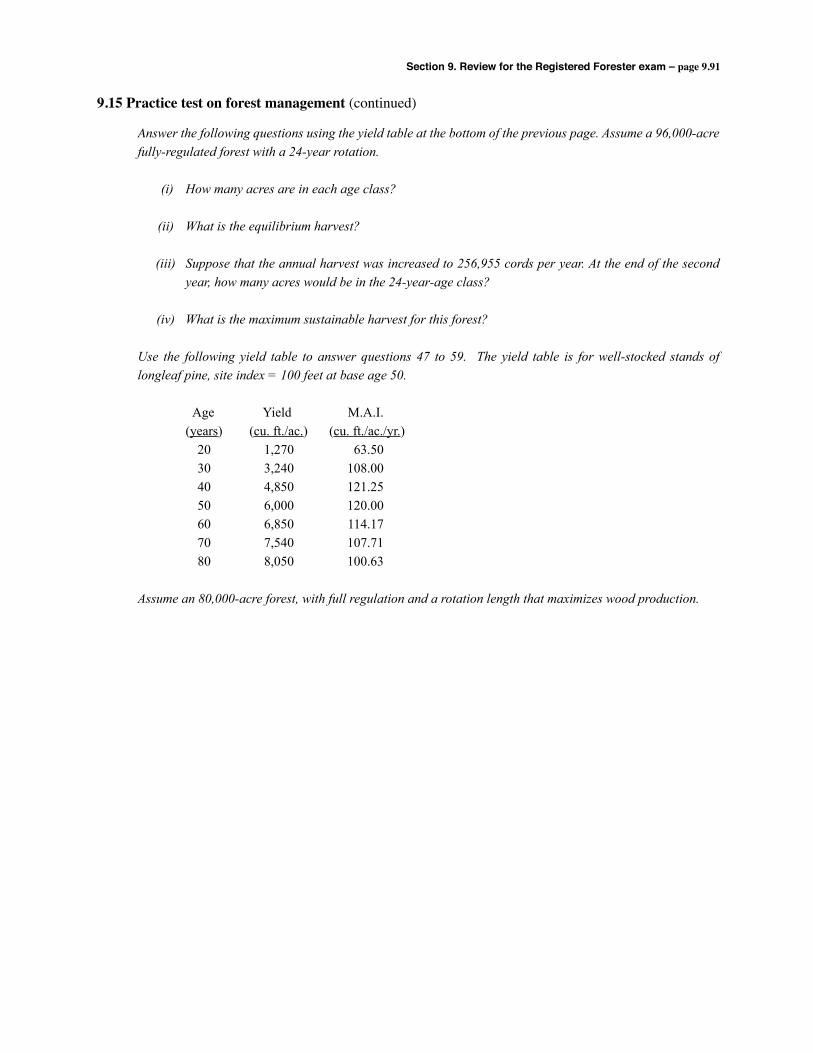
Section 9. Review for the Registered Forester exam – page 9.91
9.15 Practice test on forest management (continued)
Answer the following questions using the yield table at the bottom of the previous page. Assume a 96,000-acre fully-regulated forest with a 24-year rotation.
(i) How many acres are in each age class?
(ii) What is the equilibrium harvest?
(iii) Suppose that the annual harvest was increased to 256,955 cords per year. At the end of the second year, how many acres would be in the 24-year-age class?
(iv) What is the maximum sustainable harvest for this forest?
Use the following yield table to answer questions 47 to 59. The yield table is for well-stocked stands of longleaf pine, site index = 100 feet at base age 50.
Age Yield M.A.I. (years) (cu. ft./ac.) (cu. ft./ac./yr.) 20 1,270 63.50 30 3,240 108.00 40 4,850 121.25 50 6,000 120.00 60 6,850 114.17 70 7,540 107.71 80 8,050 100.63
Assume an 80,000-acre forest, with full regulation and a rotation length that maximizes wood production.
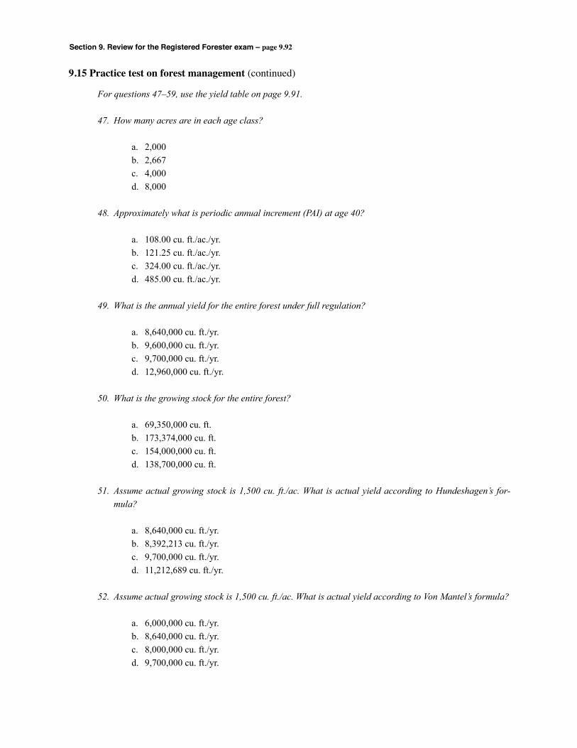
Section 9. Review for the Registered Forester exam – page 9.92
9.15 Practice test on forest management (continued)
For questions 47–59, use the yield table on page 9.91.
47. How many acres are in each age class?
a. 2,000 b. 2,667 c. 4,000 d. 8,000
48. Approximately what is periodic annual increment (PAI) at age 40?
a. 108.00 cu. ft./ac./yr. b. 121.25 cu. ft./ac./yr. c. 324.00 cu. ft./ac./yr. d. 485.00 cu. ft./ac./yr.
49. What is the annual yield for the entire forest under full regulation?
a. 8,640,000 cu. ft./yr. b. 9,600,000 cu. ft./yr. c. 9,700,000 cu. ft./yr. d. 12,960,000 cu. ft./yr.
50. What is the growing stock for the entire forest?
a. 69,350,000 cu. ft. b. 173,374,000 cu. ft. c. 154,000,000 cu. ft. d. 138,700,000 cu. ft.
51. Assume actual growing stock is 1,500 cu. ft./ac. What is actual yield according to Hundeshagen’s for-mula?
a. 8,640,000 cu. ft./yr. b. 8,392,213 cu. ft./yr. c. 9,700,000 cu. ft./yr. d. 11,212,689 cu. ft./yr.
52. Assume actual growing stock is 1,500 cu. ft./ac. What is actual yield according to Von Mantel’s formula?
a. 6,000,000 cu. ft./yr. b. 8,640,000 cu. ft./yr. c. 8,000,000 cu. ft./yr. d. 9,700,000 cu. ft./yr.

Section 9. Review for the Registered Forester exam – page 9.93
9.15 Practice test on forest management (continued)
53. Redo problem 52 using Von Mantel’s modified formula. What is actual yield for the entire forest?
a. 8,000,000 cu. ft./yr. b. 8,640,000 cu. ft./yr. c. 9,600,000 cu. ft./yr. d. 9,700,000 cu. ft./yr.
54. Assume the forest above has growing stock of 160,000,000 cu. ft. Desired growing stock is 138,700,000 cu. ft. Annual increment is 100 cu. ft./ac./yr. Over a 5-year adjustment period, what is annual cut according to the Austrian formula?
a. 8,000,000 cu. ft./yr. b. 12,060,000 cu. ft./yr. c. 12,260,000 cu. ft./yr. d. 12,960,000 cu. ft./yr.
55. Assume the forest can be broken into two portions, one to be cut and one to remain uncut. The cut portion has a 6% growth rate, the uncut portion has an 8% growth rate. The forester desires to convert the cut portion over a 10-year adjustment period. Assume: GR = future or desired growing stock = 1,733.75 cu. ft./ac. GA = present or actual growing stock = 2,000.00 cu. ft./ac. What is the annual cut using Meyer’s Amortization Formula?
a. 196 cu. ft./ac./yr. b. 213 cu. ft./ac./yr. c. 160 cu. ft./ac./yr. d. 139 cu. ft./ac./yr.
56. Assume the volume of overmature timber is 21,300,000 cu. ft. and annual increment is 100 cu. ft./ac./yr. Using Hanzlik’s formula, what is annual cut?
a. 8,392,213 cu. ft./yr. b. 8,532,500 cu. ft./yr. c. 8,260,000 cu. ft./yr. d. 8,600,000 cu. ft./yr.
57. Assume this same forest has a rotation age of 50 years. What is the annual yield?
a. 8,000,000 cu. ft./yr. b. 8,640,000 cu. ft./yr. c. 9,600,000 cu. ft./yr. d. 9,700,000 cu. ft./yr.

Section 9. Review for the Registered Forester exam – page 9.94
9.15 Practice test on forest management (continued)
58. Now assume you want to move the age class distribution on the forest to a fully-regulated condition with a rotation age of 40 years. What is the longest time period required for the conversion?
a. 20 years b. 30 years c. 40 years d. 50 years
59. During the conversion from a 50-year to a 40-year rotation, what will the annual harvest be in year 3? (Use linear interpolation to obtain yield table value.)
a. 11,862,000 cu. ft. b. 12,960,000 cu. ft. c. 11,908,000 cu. ft. d. 11,954,000 cu. ft.
60. A forest contains two even-aged stands with the following areas and ages:
Area Age Stand (acres) (years) I 620 20 II 380 30
Assuming the oldest stand is cut first, what will the total harvest be in the tenth year if the rotation age is 25 years, a harvest occurs every year, and full regulation is desired. The yield table for the forest is below:
Age Yield (years) (cords/acre) 0 0 10 4 15 12 20 20 25 30 30 40 35 45 40 50 45 53 50 55
a. 800 cords b. 1,600 cords c. 1,800 cords d. 2,000 cords
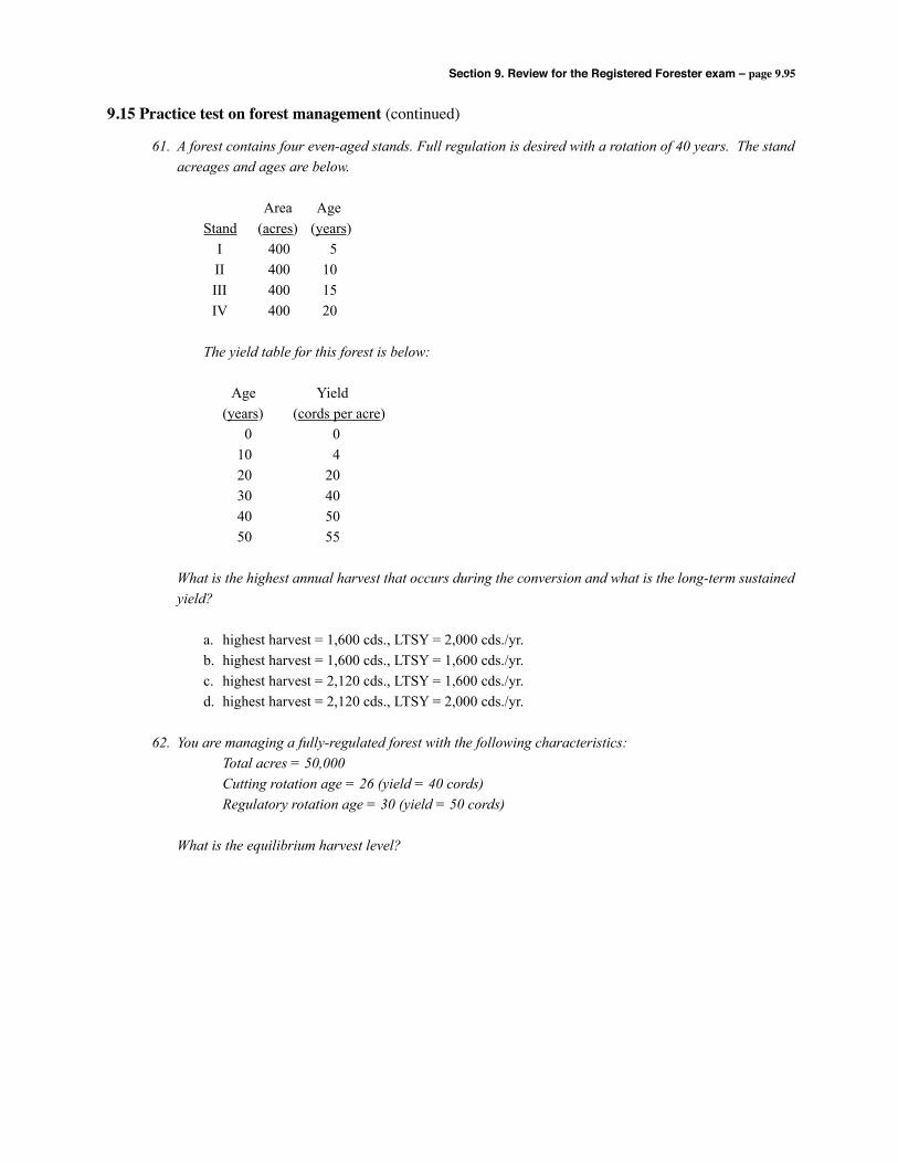
Section 9. Review for the Registered Forester exam – page 9.95
9.15 Practice test on forest management (continued)
61. A forest contains four even-aged stands. Full regulation is desired with a rotation of 40 years. The stand acreages and ages are below.
Area Age Stand (acres) (years) I 400 5 II 400 10 III 400 15 IV 400 20
The yield table for this forest is below:
Age Yield (years) (cords per acre) 0 0 10 4 20 20 30 40 40 50 50 55
What is the highest annual harvest that occurs during the conversion and what is the long-term sustained yield?
a. highest harvest = 1,600 cds., LTSY = 2,000 cds./yr. b. highest harvest = 1,600 cds., LTSY = 1,600 cds./yr. c. highest harvest = 2,120 cds., LTSY = 1,600 cds./yr. d. highest harvest = 2,120 cds., LTSY = 2,000 cds./yr.
62. You are managing a fully-regulated forest with the following characteristics: Total acres = 50,000 Cutting rotation age = 26 (yield = 40 cords) Regulatory rotation age = 30 (yield = 50 cords)
What is the equilibrium harvest level?
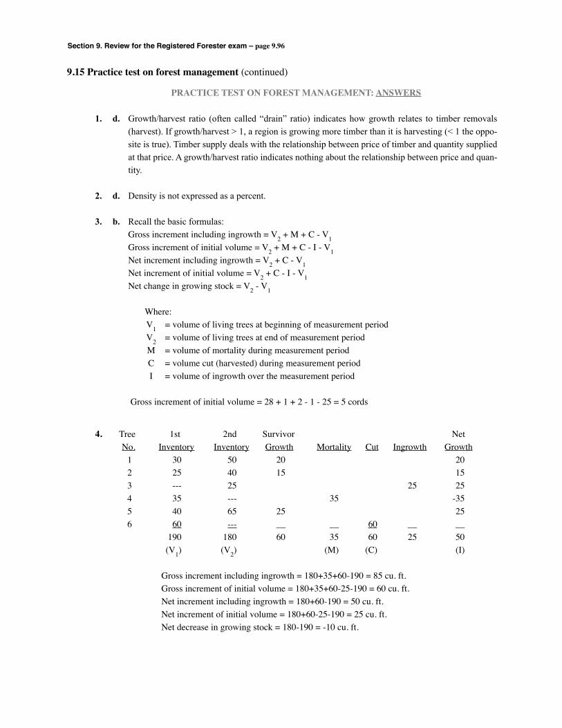
Section 9. Review for the Registered Forester exam – page 9.96
9.15 Practice test on forest management (continued)
PRACTICE TEST ON FOREST MANAGEMENT: ANSWERS
1. d. Growth/harvest ratio (often called “drain” ratio) indicates how growth relates to timber removals (harvest). If growth/harvest > 1, a region is growing more timber than it is harvesting (< 1 the oppo-site is true). Timber supply deals with the relationship between price of timber and quantity supplied at that price. A growth/harvest ratio indicates nothing about the relationship between price and quan-tity.
2. d. Density is not expressed as a percent.
3. b. Recall the basic formulas: Gross increment including ingrowth = V2 + M + C - V1 Gross increment of initial volume = V2 + M + C - I - V1 Net increment including ingrowth = V2 + C - V1 Net increment of initial volume = V2 + C - I - V1 Net change in growing stock = V2 - V1 Where: V1 = volume of living trees at beginning of measurement period V2 = volume of living trees at end of measurement period M = volume of mortality during measurement period C = volume cut (harvested) during measurement period I = volume of ingrowth over the measurement period
Gross increment of initial volume = 28 + 1 + 2 - 1 - 25 = 5 cords
4. Tree 1st 2nd Survivor Net No. Inventory Inventory Growth Mortality Cut Ingrowth Growth 1 30 50 20 20 2 25 40 15 15 3 --- 25 25 25 4 35 --- 35 -35 5 40 65 25 25 6 60 --- __ __ 60 __ __ 190 180 60 35 60 25 50 (V1) (V2) (M) (C) (I)
Gross increment including ingrowth = 180+35+60-190 = 85 cu. ft. Gross increment of initial volume = 180+35+60-25-190 = 60 cu. ft. Net increment including ingrowth = 180+60-190 = 50 cu. ft. Net increment of initial volume = 180+60-25-190 = 25 cu. ft. Net decrease in growing stock = 180-190 = -10 cu. ft.
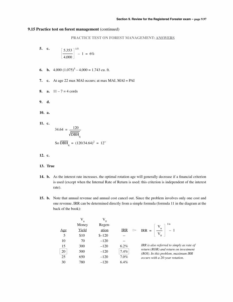
Section 9. Review for the Registered Forester exam – page 9.97
9.15 Practice test on forest management (continued)
PRACTICE TEST ON FOREST MANAGEMENT: ANSWERS
5. c.
6. b. 4,000 (1.075)5 – 4,000 = 1,743 cu. ft.
7. c. At age 22 max MAI occurs; at max MAI, MAI = PAI
8. a. 11 – 7 = 4 cords
9. d.
10. a.
11. c.
12. c.
13. True
14. b. As the interest rate increases, the optimal rotation age will generally decrease if a financial criterion is used (except when the Internal Rate of Return is used; this criterion is independent of the interest rate).
15. b. Note that annual revenue and annual cost cancel out. Since the problem involves only one cost and one revenue, IRR can be determined directly from a simple formula (formula 11 in the diagram at the back of the book):
Vn V0 Money Regen- Age Yield ation IRR 5 $10 $–120 -- 10 70 –120 -- 15 300 –120 6.2% 20 500 –120 7.4% 25 650 –120 7.0% 30 780 –120 6.4%
34.64 = 120
DBHq
So DBHq = (120/34.64)2 = 12”
5,353
4,000
1/5
– 1 = 6%
IRR =Vn
V0
1/n
– 1
IRR is also referred to simply as rate of return (ROR) and return on investment (ROI). In this problem, maximum IRR occurs with a 20-year rotation.
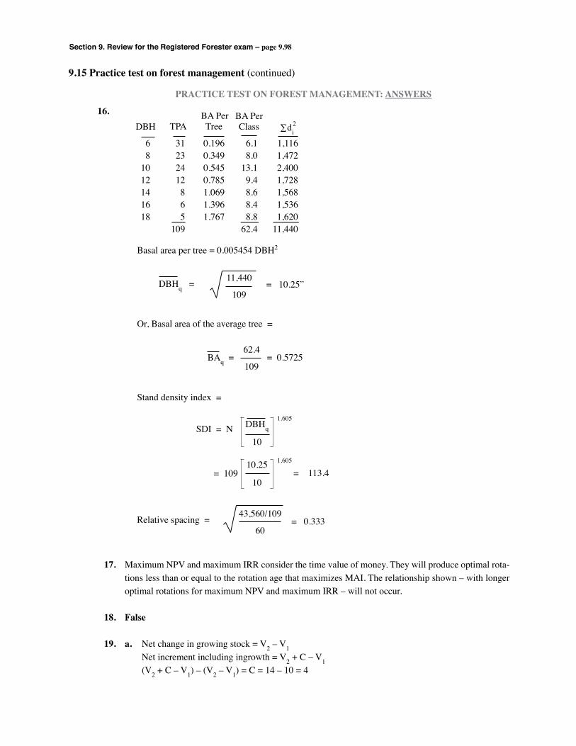
Section 9. Review for the Registered Forester exam – page 9.98
9.15 Practice test on forest management (continued)
PRACTICE TEST ON FOREST MANAGEMENT: ANSWERS
16.
6 31 0.196 6.1 1,116 8 23 0.349 8.0 1,472 10 24 0.545 13.1 2,400 12 12 0.785 9.4 1,728 14 8 1.069 8.6 1,568 16 6 1.396 8.4 1,536 18 5 1.767 8.8 1,620 109 62.4 11,440
DBH TPA Tree Class ∑di2
BA Per BA Per
Basal area per tree = 0.005454 DBH2
Or, Basal area of the average tree =
Stand density index =
Relative spacing =
DBHq =11,440
109= 10.25”
BAq = = 0.572562.4
109
SDI = N DBHq
10
1.605
= 10910.25
10
1.605
= 113.4
43,560/109
60= 0.333
17. Maximum NPV and maximum IRR consider the time value of money. They will produce optimal rota-tions less than or equal to the rotation age that maximizes MAI. The relationship shown – with longer optimal rotations for maximum NPV and maximum IRR – will not occur.
18. False
19. a. Net change in growing stock = V2 – V1 Net increment including ingrowth = V2 + C – V1 (V2 + C – V1) – (V2 – V1) = C = 14 – 10 = 4
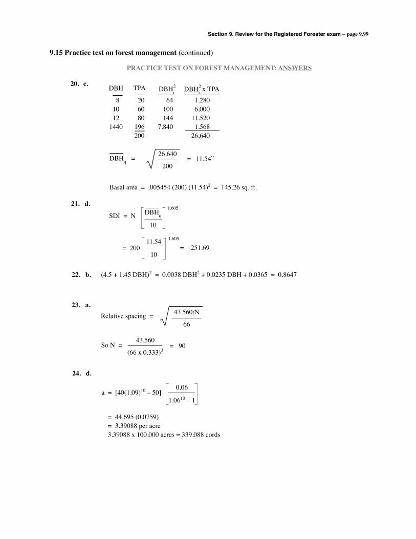
Section 9. Review for the Registered Forester exam – page 9.99
9.15 Practice test on forest management (continued)
PRACTICE TEST ON FOREST MANAGEMENT: ANSWERS
20. c.
DBHq =26,640
200= 11.54”
SDI = N DBHq
10
1.605
= 20011.54
10
1.605
= 251.69
8 20 64 1,280 10 60 100 6,000 12 80 144 11,520 14 40 196 7,840 1,568 200 26,640
DBH TPA DBHi2 DBHi
2 x TPA
Basal area = .005454 (200) (11.54)2 = 145.26 sq. ft.
21. d.
22. b. (4.5 + 1.45 DBH)2 = 0.0038 DBH2 + 0.0235 DBH + 0.0365 = 0.8647
23. a.43,560/N
66Relative spacing =
= 9043,560
(66 x 0.333)2So N =
24. d.
a = [40(1.09)10 – 50]0.06
1.0610 – 1
= 44.695 (0.0759)= 3.39088 per acre3.39088 x 100,000 acres = 339,088 cords
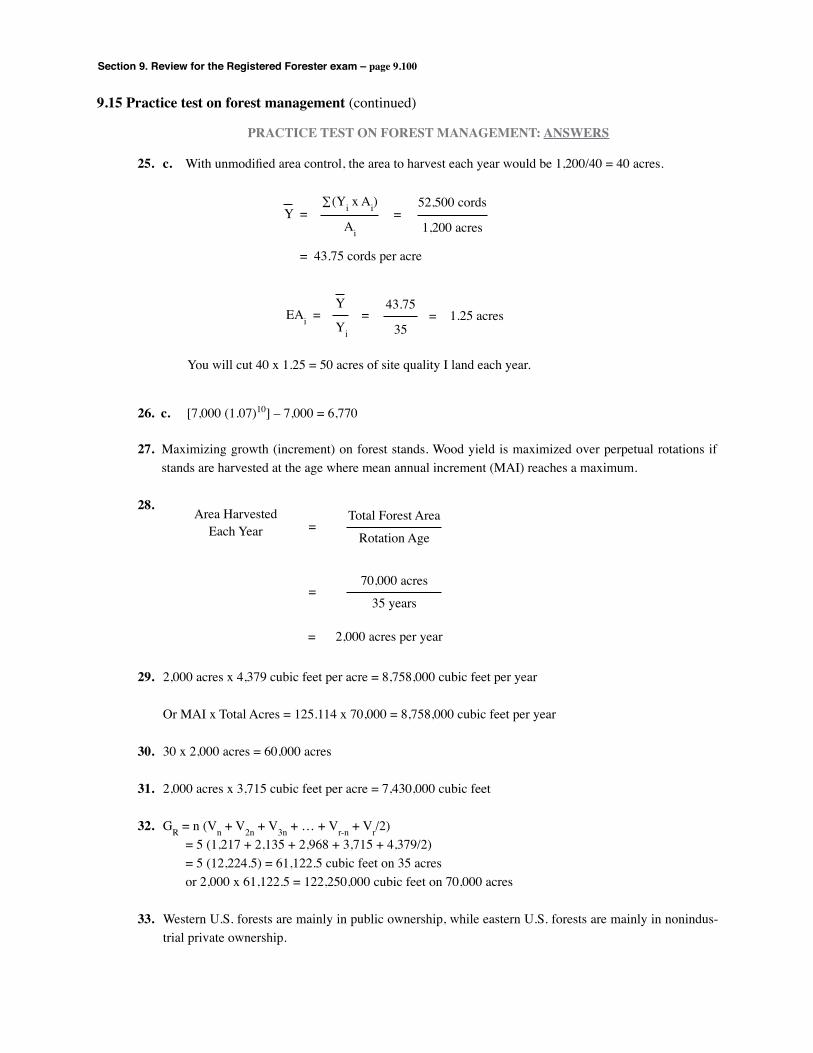
Section 9. Review for the Registered Forester exam – page 9.100
9.15 Practice test on forest management (continued)
PRACTICE TEST ON FOREST MANAGEMENT: ANSWERS
25. c. With unmodified area control, the area to harvest each year would be 1,200/40 = 40 acres.
Y =∑(Yi x Ai)
Ai
52,500 cords
1,200 acres=
= 43.75 cords per acre
EAi =Y
Yi
=43.75
35= 1.25 acres
You will cut 40 x 1.25 = 50 acres of site quality I land each year.
26. c. [7,000 (1.07)10] – 7,000 = 6,770
27. Maximizing growth (increment) on forest stands. Wood yield is maximized over perpetual rotations if stands are harvested at the age where mean annual increment (MAI) reaches a maximum.
28.Area Harvested
Each YearTotal Forest Area
Rotation Age=
70,000 acres
35 years=
= 2,000 acres per year
29. 2,000 acres x 4,379 cubic feet per acre = 8,758,000 cubic feet per year
Or MAI x Total Acres = 125.114 x 70,000 = 8,758,000 cubic feet per year
30. 30 x 2,000 acres = 60,000 acres
31. 2,000 acres x 3,715 cubic feet per acre = 7,430,000 cubic feet
32. GR = n (Vn + V2n + V3n + … + Vr-n + Vr/2) = 5 (1,217 + 2,135 + 2,968 + 3,715 + 4,379/2) = 5 (12,224.5) = 61,122.5 cubic feet on 35 acres or 2,000 x 61,122.5 = 122,250,000 cubic feet on 70,000 acres
33. Western U.S. forests are mainly in public ownership, while eastern U.S. forests are mainly in nonindus-trial private ownership.
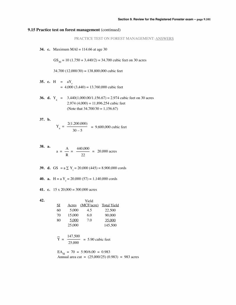
Section 9. Review for the Registered Forester exam – page 9.101
9.15 Practice test on forest management (continued)
PRACTICE TEST ON FOREST MANAGEMENT: ANSWERS
34. c. Maximum MAI = 114.66 at age 30
GS30 = 10 (1,750 + 3,440/2) = 34,700 cubic feet on 30 acres 34,700 (12,000/30) = 138,800,000 cubic feet
35. c. H = aYr = 4,000 (3,440) = 13,760,000 cubic feet
36. d. Ya = 3,440(1,000.00/1,156.67) = 2,974 cubic feet on 30 acres 2,974 (4,000) = 11,896,254 cubic feet (Note that 34,700/30 = 1,156.67)
37. b.
38. a.
39. d. GS = a ∑ Yi = 20,000 (445) = 8,900,000 cords
40. a. H = a Yr = 20,000 (57) = 1,140,000 cords
41. c. 15 x 20,000 = 300,000 acres
42.
2(1,200,000)
30 – 5Ya = = 9,600,000 cubic feet
a = = = 20,000 acresA
R
440,000
22
SI607080
Acres5,000
15,0005,000
25,000
(MCF/acre)4.56.07.0
Total Yield22,50090,00035,000145,500
Yield
Y =147,500
25,000= 5.90 cubic feet
EASI = 70 = 5.90/6.00 = 0.983Annual area cut = (25,000/25) (0.983) = 983 acres
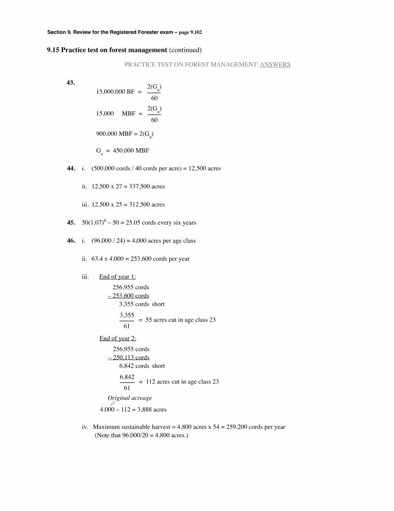
Section 9. Review for the Registered Forester exam – page 9.102
9.15 Practice test on forest management (continued)
PRACTICE TEST ON FOREST MANAGEMENT: ANSWERS
43. 15,000,000 BF =
2(Ga)
60
15,000 MBF =2(Ga)
60
900,000 MBF = 2(Ga)
Ga = 450,000 MBF
44. i. (500,000 cords / 40 cords per acre) = 12,500 acres
ii. 12,500 x 27 = 337,500 acres
iii. 12,500 x 25 = 312,500 acres
45. 50(1.07)6 – 50 = 25.05 cords every six years
46. i. (96,000 / 24) = 4,000 acres per age class
ii. 63.4 x 4,000 = 253,600 cords per year
iii. End of year 1:
256,955 cords– 253,600 cords
3,355 cords short
3,355
61= 55 acres cut in age class 23
End of year 2:
256,955 cords– 250,113 cords
6,842 cords short
6,842
61= 112 acres cut in age class 23
4,000 – 112 = 3,888 acres
Original acreage
iv. Maximum sustainable harvest = 4,800 acres x 54 = 259,200 cords per year (Note that 96,000/20 = 4,800 acres.)
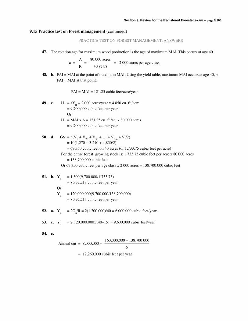
Section 9. Review for the Registered Forester exam – page 9.103
9.15 Practice test on forest management (continued)
PRACTICE TEST ON FOREST MANAGEMENT: ANSWERS
47. The rotation age for maximum wood production is the age of maximum MAI. This occurs at age 40.
48. b. PAI = MAI at the point of maximum MAI. Using the yield table, maximum MAI occurs at age 40, so PAI = MAI at that point:
PAI = MAI = 121.25 cubic feet/acre/year
49. c. H = aYR = 2,000 acres/year x 4,850 cu. ft./acre = 9,700,000 cubic feet per year Or, H = MAI x A = 121.25 cu. ft./ac. x 80,000 acres = 9,700,000 cubic feet per year
50. d. GS = n(Vn + V2n + V3n + … + Vr–n + Vr/2) = 10(1,270 + 3,240 + 4,850/2) = 69,350 cubic feet on 40 acres (or 1,733.75 cubic feet per acre) For the entire forest, growing stock is: 1,733.75 cubic feet per acre x 80,000 acres = 138,700,000 cubic feet Or 69,350 cubic feet per age class x 2,000 acres = 138,700,000 cubic feet
51. b. Ya = 1,500(9,700,000/1,733.75) = 8,392,213 cubic feet per year Or, Ya = 120,000,000(9,700,000/138,700,000) = 8,392,213 cubic feet per year
52. a. Ya = 2Ga/R = 2(1,200,000)/40 = 6,000,000 cubic feet/year
53. c. Ya = 2(120,000,000)/(40–15) = 9,600,000 cubic feet/year
54. c.
a = = = 2,000 acres per age classA
R
80,000 acres
40 years
Annual cut = 8,000,000 +
= 12,260,000 cubic feet per year
160,000,000 – 138,700,000
5

Section 9. Review for the Registered Forester exam – page 9.104
9.15 Practice test on forest management (continued)
PRACTICE TEST ON FOREST MANAGEMENT: ANSWERS
55. a.
Note that the expression on the far right is commonly called the sinking fund formula (it’s formula 7 on the last page of the workbook). This means 196 cubic feet/acre/year at a 6% growth rate is equal to a harvest of 2,584.10 cubic feet (or the Future Value of 196 cubic feet per year at 6% interest is 2,584 cubic feet). On the entire forest, annual cut is 196 cubic feet x 80,000 acres = 15,680,000 cubic feet per year over the 10 years.
56. b.
57. c. H = aYR = 1,600 acres x 6,000 cubic feet per acre = 9,600,000 cubic feet per year Or, H = MAI x A = 120.00 cubic feet per acre per year x 80,000 acres = 9,600,000 cubic feet per year
58. c. 40 years. You will cut 1/40th of the forest each year, so the forest must be fully converted by the end of 40 years.
59. a. In year 1, harvest: 1,600 acres of the 50-year age class, and 400 acres of the 49-year age class.
In year 2, harvest: 1,200 acres of the 50-year age class, and 800 acres of the 49-year age class.
In year 3, harvest: 800 acres of the 50-year age class, and 1,200 acres of the 49-year age class.
800 acres x 6,000 cu.ft./acre = 4,800,000 cu.ft. 1,200 acres x 5,885 cu.ft./acre= 7,062,000 cu.ft. 11,862,000 cu.ft.
a = [2,000(1.08)10 – 1,733.75].06
(1.06)10 – 1
= (2,584.10)(0.07587) = 196 cubic feet/ac./yr.
Annual cut = 8,000,000 +21,300,000
40= 8,532,500 cubic feet per year
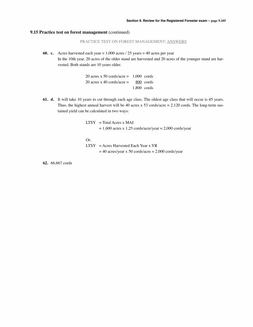
Section 9. Review for the Registered Forester exam – page 9.105
9.15 Practice test on forest management (continued)
PRACTICE TEST ON FOREST MANAGEMENT: ANSWERS
60. c. Acres harvested each year = 1,000 acres / 25 years = 40 acres per year In the 10th year, 20 acres of the older stand are harvested and 20 acres of the younger stand are har-
vested. Both stands are 10 years older.
20 acres x 50 cords/acre = 1,000 cords 20 acres x 40 cords/acre = 800 cords 1,800 cords
61. d. It will take 10 years to cut through each age class. The oldest age class that will occur is 45 years. Thus, the highest annual harvest will be 40 acres x 53 cords/acre = 2,120 cords. The long-term sus-tained yield can be calculated in two ways:
LTSY = Total Acres x MAI = 1,600 acres x 1.25 cords/acre/year = 2,000 cords/year
Or, LTSY = Acres Harvested Each Year x YR = 40 acres/year x 50 cords/acre = 2,000 cords/year
62. 66,667 cords


Section 10. Solutions to problems – page 10.1
“Errors, like straws, upon the surface flow;he who would search for pearls must dive below.”
– John Dryden (1678)
Section
10 Solutionsto problems
Problem 3.1
A 12-year terminating annual series. Calculate V0 using 6% …
V0 = $1,600(1.06)12 – 1
.06(1.06)12= $13,414.15
0 1 2 3 ……
…
……
11 1210
$1,60
0$1
,600
$1,60
0$1
,600
$1,60
0
$1,60
0
This answer can also be calculated using the payment key on a financial calculator; this can be done by entering the $1,600 as a 12-year series of payments and “computing” the present value.
1. Basics of compound interest
2. Four basic formulas
3. Twelve formulas
4. Financial criteria
5. Financial analysis concepts
6. Inflation and taxes
7. Forest valuation
8. An example computer program
9. Review for the Registered
Forester exam
10. Solutions to problems
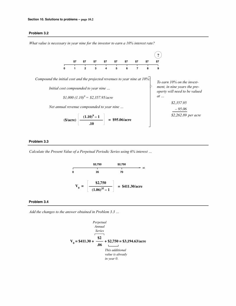
Section 10. Solutions to problems – page 10.2
Problem 3.2
What value is necessary in year nine for the investor to earn a 10% interest rate?
Compound the initial cost and the projected revenues to year nine at 10%:
Initial cost compounded to year nine …
$1,000 (1.10)9 = $2,357.95/acre
Net annual revenue compounded to year nine …
($/acre)(1.10)9 – 1
.10= $95.06/acre
0 1 2 3 4 5 6 7 8 9
$7 $7 $7 $7 $7 $7 $7 $7 $7
?
To earn 10% on the invest-ment, in nine years the pre-operty will need to be valued at …
$2,357.95– 95.06
$2,262.89 per acre
Problem 3.3
Calculate the Present Value of a Perpetual Periodic Series using 6% interest …
8
0 35 70
$2,750 $2,750
V0 =$2,750
(1.06)35 – 1= $411.30/acre
Problem 3.4
Add the changes to the answer obtained in Problem 3.3 …
V0 = $411.30 + + $2,750 = $3,194.63/acre$2
.06This additional value is already in year 0.
PerpetualAnnualSeries

Section 10. Solutions to problems – page 10.3
Problem 3.5
Calculate the Present Value of a Terminating Annual Series using 10% interest …
0 1 2 3 4 5 6 7 8
$3,00
0$3
,000
$3,00
0$3
,000
$3,00
0$3
,000
$3,00
0$3
,000
V0 = $3,000(1.10)8 – 1
.10(1.10)8= $16,004.78
Problem 3.6
Calculate the Present Value of a Terminating Annual Series using 9% interest …
0 1 2 3 ……
…
……
24 2523
$12 $12 $12 $12 $12 $12 $12
The 25-year series begins in year zero, but the terminating annual series formulas assume the first value occurs at the end of year one. We therefore add $12 to the result we obtain with the Present Value formula. The $12 that’s unaccounted for by the formula is already in year 0, so discounting isn’t necessary.
Assuming the series terminates in year 25, total Present Value is:
Assuming the series goes on forever, the total Present Value is:
V0 = $12 + = $138.32
V0 = $12 + $12(1.095)25 – 1
.095(1.095)25= $125.25
$12
.095
Problem 3.7
Calculate the Present Value of a Terminating Annual Series, plus a single sum using 7% interest …
0 1 2 3 4 5 6 7 8 9 10
$4,00
0$4
,000
$4,00
0$4
,000
$4,00
0$4
,000
$4,00
0$4
,000
$4,00
0
$10,000
V0 = $4,000(1.07)9 – 1
.07(1.07)9= $31,144.42+
$10,000
1.0710
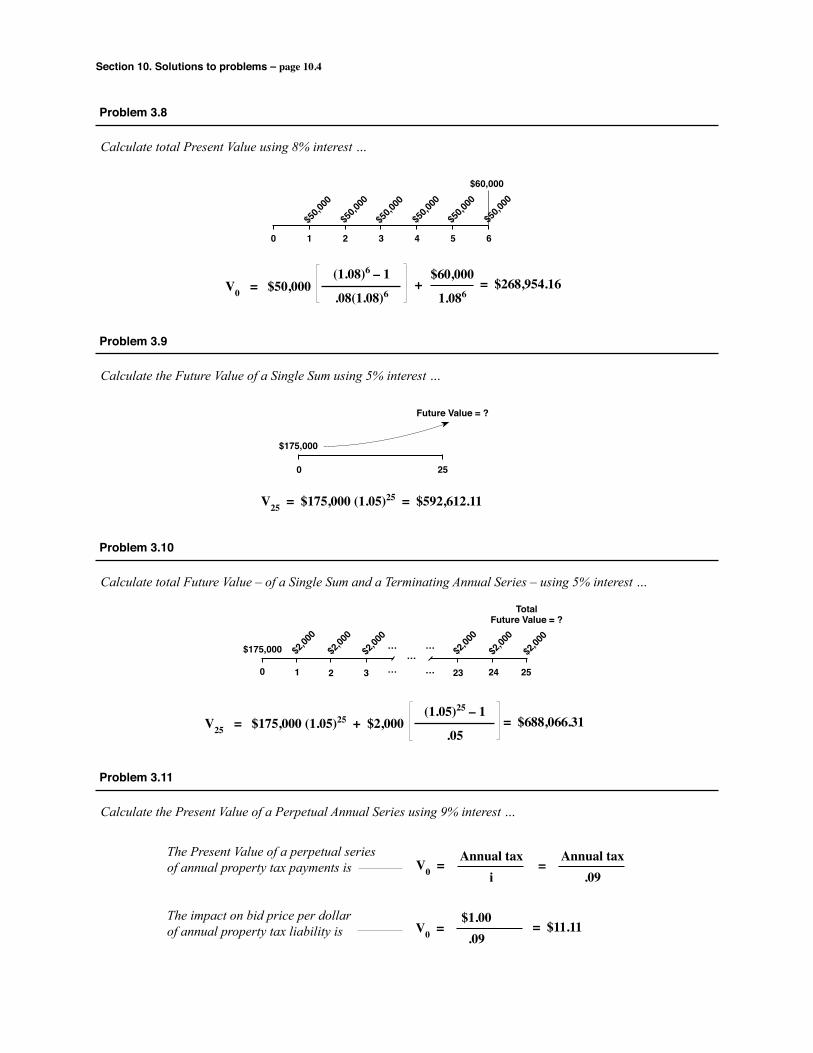
Section 10. Solutions to problems – page 10.4
Problem 3.8
Calculate total Present Value using 8% interest …
0 1 2 3 4 5 6
$50,0
00
$50,0
00
$50,0
00
$50,0
00
$50,0
00
$50,0
00$60,000
V0 = $50,000(1.08)6 – 1
.08(1.08)6= $268,954.16+
$60,000
1.086
Problem 3.9
Calculate the Future Value of a Single Sum using 5% interest …
0 25
$175,000
Future Value = ?
V25 = $175,000 (1.05)25 = $592,612.11
Problem 3.10
Calculate total Future Value – of a Single Sum and a Terminating Annual Series – using 5% interest …
V25 = $175,000 (1.05)25 + $2,000(1.05)25 – 1
.05= $688,066.31
0 1 2 3 ……
…
……
24 2523
$2,00
0$2
,000
$2,00
0$2
,000
$2,00
0
$2,00
0
TotalFuture Value = ?
$175,000
Problem 3.11
Calculate the Present Value of a Perpetual Annual Series using 9% interest …
The Present Value of a perpetual seriesof annual property tax payments is
The impact on bid price per dollarof annual property tax liability is
V0 =Annual tax
iAnnual tax
.09=
V0 =$1.00.09
= $11.11
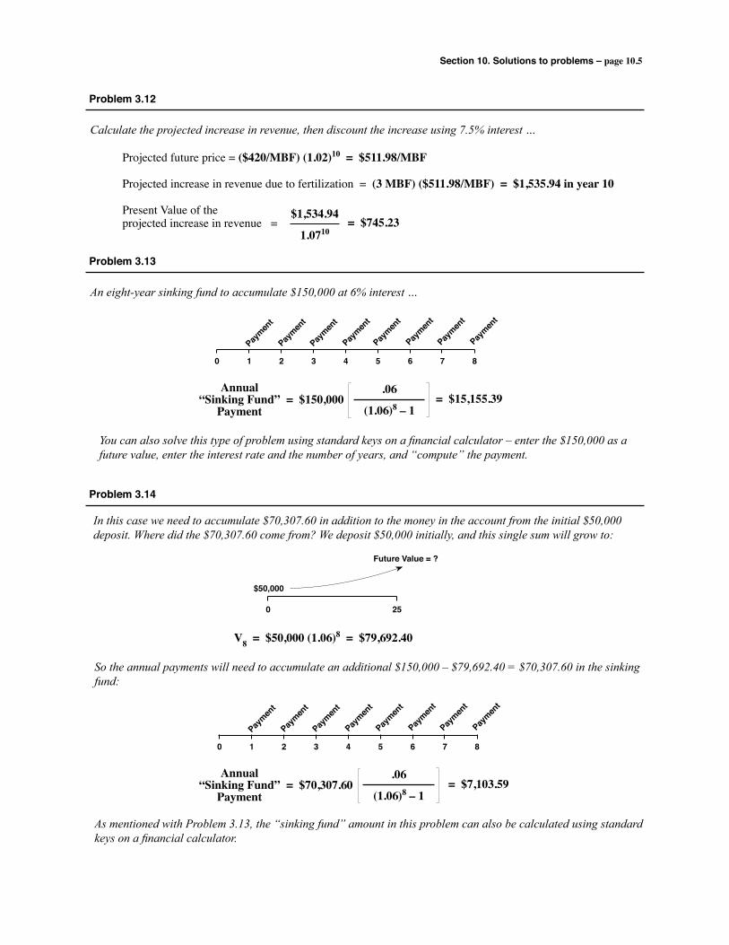
Section 10. Solutions to problems – page 10.5
Problem 3.12
Calculate the projected increase in revenue, then discount the increase using 7.5% interest …
Projectedfutureprice=($420/MBF) (1.02)10 = $511.98/MBF
Projectedincreaseinrevenueduetofertilization= (3 MBF) ($511.98/MBF) = $1,535.94 in year 10
PresentValueoftheprojectedincreaseinrevenue=
$1,534.94
1.0710= $745.23
Problem 3.13
An eight-year sinking fund to accumulate $150,000 at 6% interest …
0 1 2 3 4 5 6 7 8
Paymen
t
Paymen
t
Paymen
t
Paymen
t
Paymen
t
Paymen
t
Paymen
t
Paymen
t
.06
(1.06)8 – 1= $15,155.39= $150,000
Annual“Sinking Fund”
Payment
You can also solve this type of problem using standard keys on a financial calculator – enter the $150,000 as a future value, enter the interest rate and the number of years, and “compute” the payment.
Problem 3.14
0 25
$50,000
Future Value = ?
V8 = $50,000 (1.06)8 = $79,692.40
In this case we need to accumulate $70,307.60 in addition to the money in the account from the initial $50,000 deposit. Where did the $70,307.60 come from? We deposit $50,000 initially, and this single sum will grow to:
So the annual payments will need to accumulate an additional $150,000 – $79,692.40 = $70,307.60 in the sinking fund:
0 1 2 3 4 5 6 7 8
Paymen
t
Paymen
t
Paymen
t
Paymen
t
Paymen
t
Paymen
t
Paymen
t
Paymen
t
.06
(1.06)8 – 1= $7,103.59= $70,307.60
Annual“Sinking Fund”
Payment
As mentioned with Problem 3.13, the “sinking fund” amount in this problem can also be calculated using standard keys on a financial calculator.
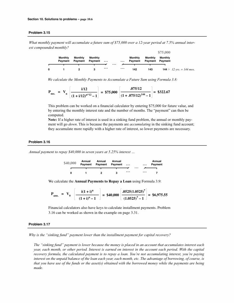
Section 10. Solutions to problems – page 10.6
Problem 3.15
What monthly payment will accumulate a future sum of $75,000 over a 12-year period at 7.5% annual inter-est compounded monthly?
0 1 2 3 142 143 144… ……
…… Monthly Monthly Monthly Monthly Monthly Monthly Payment Payment Payment Payment Payment Payment
$75,000
12 yrs. = 144 mos.
Pmo. = Vni/12
(1 + i/12)n*12 – 1= $75,000
.075/12
(1 + .075/12)144 – 1= $322.67
This problem can be worked on a financial calculator by entering $75,000 for future value, and by entering the monthly interest rate and the number of months. The “payment” can then be computed.Note: If a higher rate of interest is used in a sinking fund problem, the annual or monthly pay-ment will go down. This is because the payments are accumulating in the sinking fund account; they accumulate more rapidly with a higher rate of interest, so lower payments are necessary.
We calculate the Monthly Payments to Accumulate a Future Sum using Formula 3.8:
Problem 3.16
Annual payment to repay $40,000 in seven years at 5.25% interest …
0 1 2 3 7 … ……
…… Annual Annual Annual Annual Payment Payment Payment Payment $40,000
WecalculatetheAnnual Payments to Repay a LoanusingFormula3.9:
Pann. = V0i(1 + i)n
(1 + i)n – 1
.0525(1.0525)7
(1.0525)7 – 1= $40,000 = $6,975.55
Financialcalculatorsalsohavekeystocalculateinstallmentpayments.Problem3.16canbeworkedasshownintheexampleonpage3.31.
Problem 3.17
Why is the “sinking fund” payment lower than the installment payment for capital recovery?
The “sinking fund” payment is lower because the money is placed in an account that accumulates interest each year, each month, or other period. Interest is earned on interest in the account each period. With the capital recovery formula, the calculated payment is to repay a loan. You’re not accumulating interest, you’re paying interest on the unpaid balance of the loan each year, each month, etc. The advantage of borrowing, of course, is that you have use of the funds or the asset(s) obtained with the borrowed money while the payments are being made.
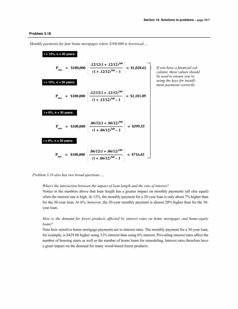
Section 10. Solutions to problems – page 10.7
Problem 3.18
Monthly payments for four home mortgages where $100,000 is borrowed …
Pmo. = $100,000.12/12(1 + .12/12)360
(1 + .12/12)360 – 1= $1,028.61
i = 12%, n = 30 years:
Pmo. = $100,000.12/12(1 + .12/12)240
(1 + .12/12)360 – 1= $1,101.09
i = 12%, n = 20 years:
Pmo. = $100,000.06/12(1 + .06/12)360
(1 + .06/12)360 – 1= $599.55
i = 6%, n = 30 years:
Pmo. = $100,000.06/12(1 + .06/12)240
(1 + .06/12)360 – 1= $716.43
i = 6%, n = 20 years:
If you have a financial cal-culator, these values should be used to ensure you’re using the keys for install-ment payments correctly.
Problem 3.18 also has two broad questions …
What’s the interaction between the impact of loan length and the rate of interest? Notice in the numbers above that loan length has a greater impact on monthly payments (all else equal)
when the interest rate is high. At 12%, the monthly payment for a 20-year loan is only about 7% higher than for the 30-year loan. At 6%, however, the 20-year monthly payment is almost 20% higher than for the 30-year loan.
How is the demand for forest products affected by interest rates on home mortgages and home-equity loans?
Note how sensitive home mortgage payments are to interest rates. The monthly payment for a 30-year loan, for example, is $429.06 higher using 12% interest than using 6% interest. Prevailing interest rates affect the number of housing starts as well as the number of home loans for remodeling. Interest rates therefore have a great impact on the demand for many wood-based forest products.
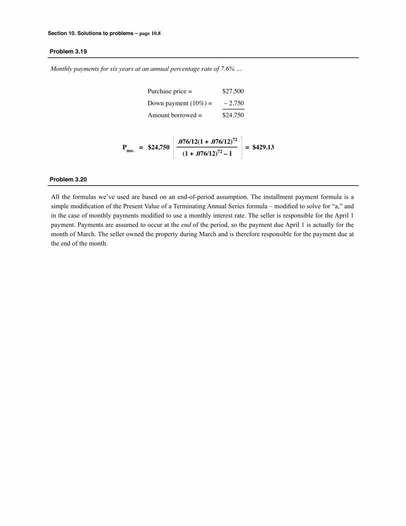
Section 10. Solutions to problems – page 10.8
Problem 3.19
Monthly payments for six years at an annual percentage rate of 7.6% …
Pmo. = $24,750.076/12(1 + .076/12)72
(1 + .076/12)72 – 1= $429.13
Purchaseprice= $27,500
Downpayment(10%)= –2,750
Amountborrowed= $24,750
Problem 3.20
All the formulas we’ve used are based on an end-of-period assumption. The installment payment formula is a simple modification of the Present Value of a Terminating Annual Series formula – modified to solve for “a,” and in the case of monthly payments modified to use a monthly interest rate. The seller is responsible for the April 1 payment. Payments are assumed to occur at the end of the period, so the payment due April 1 is actually for the month of March. The seller owned the property during March and is therefore responsible for the payment due at the end of the month.
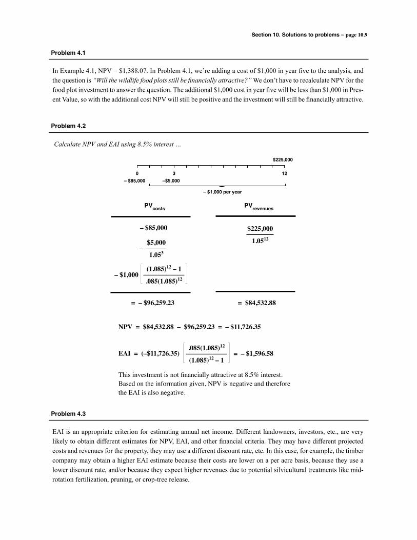
Section 10. Solutions to problems – page 10.9
Problem 4.1
In Example 4.1, NPV = $1,388.07. In Problem 4.1, we’re adding a cost of $1,000 in year five to the analysis, and the question is “Will the wildlife food plots still be financially attractive?” We don’t have to recalculate NPV for the food plot investment to answer the question. The additional $1,000 cost in year five will be less than $1,000 in Pres-ent Value, so with the additional cost NPV will still be positive and the investment will still be financially attractive.
Problem 4.2
Calculate NPV and EAI using 8.5% interest …
0 3 12– $85,000 –$5,000
$225,000
– $1,000 per year
PVcosts PVrevenues
– $85,000
$5,000
1.053
– $1,000(1.085)12 – 1
.085(1.085)12
= – $96,259.23 = $84,532.88
$225,000
1.0512
NPV = $84,532.88 – $96,259.23 = – $11,726.35
EAI = (–$11,726.35) = – $1,596.58.085(1.085)12
(1.085)12 – 1
Thisinvestmentisnotfinanciallyattractiveat8.5%interest.Basedontheinformationgiven,NPVisnegativeandthereforetheEAIisalsonegative.
Problem 4.3
EAI is an appropriate criterion for estimating annual net income. Different landowners, investors, etc., are very likely to obtain different estimates for NPV, EAI, and other financial criteria. They may have different projected costs and revenues for the property, they may use a different discount rate, etc. In this case, for example, the timber company may obtain a higher EAI estimate because their costs are lower on a per acre basis, because they use a lower discount rate, and/or because they expect higher revenues due to potential silvicultural treatments like mid-rotation fertilization, pruning, or crop-tree release.
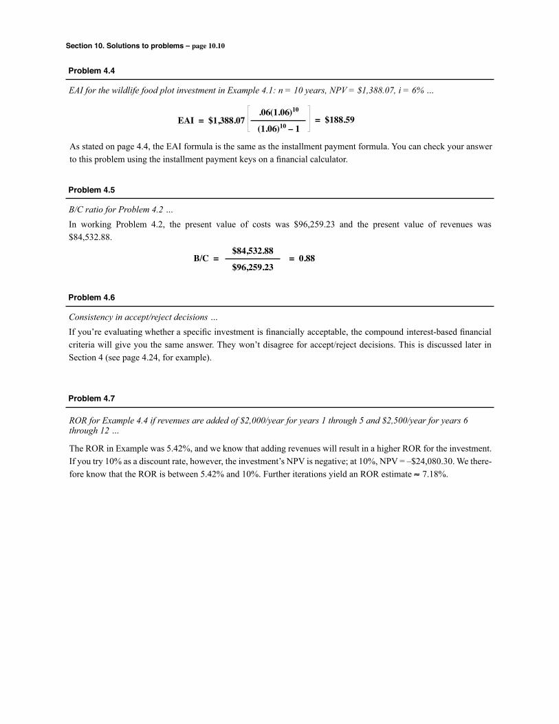
Section 10. Solutions to problems – page 10.10
Problem 4.4
As stated on page 4.4, the EAI formula is the same as the installment payment formula. You can check your answer to this problem using the installment payment keys on a financial calculator.
EAI for the wildlife food plot investment in Example 4.1: n = 10 years, NPV = $1,388.07, i = 6% …
= $188.59.06(1.06)10
(1.06)10 – 1EAI = $1,388.07
Problem 4.5
In working Problem 4.2, the present value of costs was $96,259.23 and the present value of revenues was $84,532.88.
B/C ratio for Problem 4.2 …
= 0.88$84,532.88
$96,259.23B/C =
Problem 4.6
If you’re evaluating whether a specific investment is financially acceptable, the compound interest-based financial criteria will give you the same answer. They won’t disagree for accept/reject decisions. This is discussed later in Section 4 (see page 4.24, for example).
Consistency in accept/reject decisions …
Problem 4.7
The ROR in Example was 5.42%, and we know that adding revenues will result in a higher ROR for the investment. If you try 10% as a discount rate, however, the investment’s NPV is negative; at 10%, NPV = –$24,080.30. We there-fore know that the ROR is between 5.42% and 10%. Further iterations yield an ROR estimate ≈ 7.18%.
ROR for Example 4.4 if revenues are added of $2,000/year for years 1 through 5 and $2,500/year for years 6 through 12 …
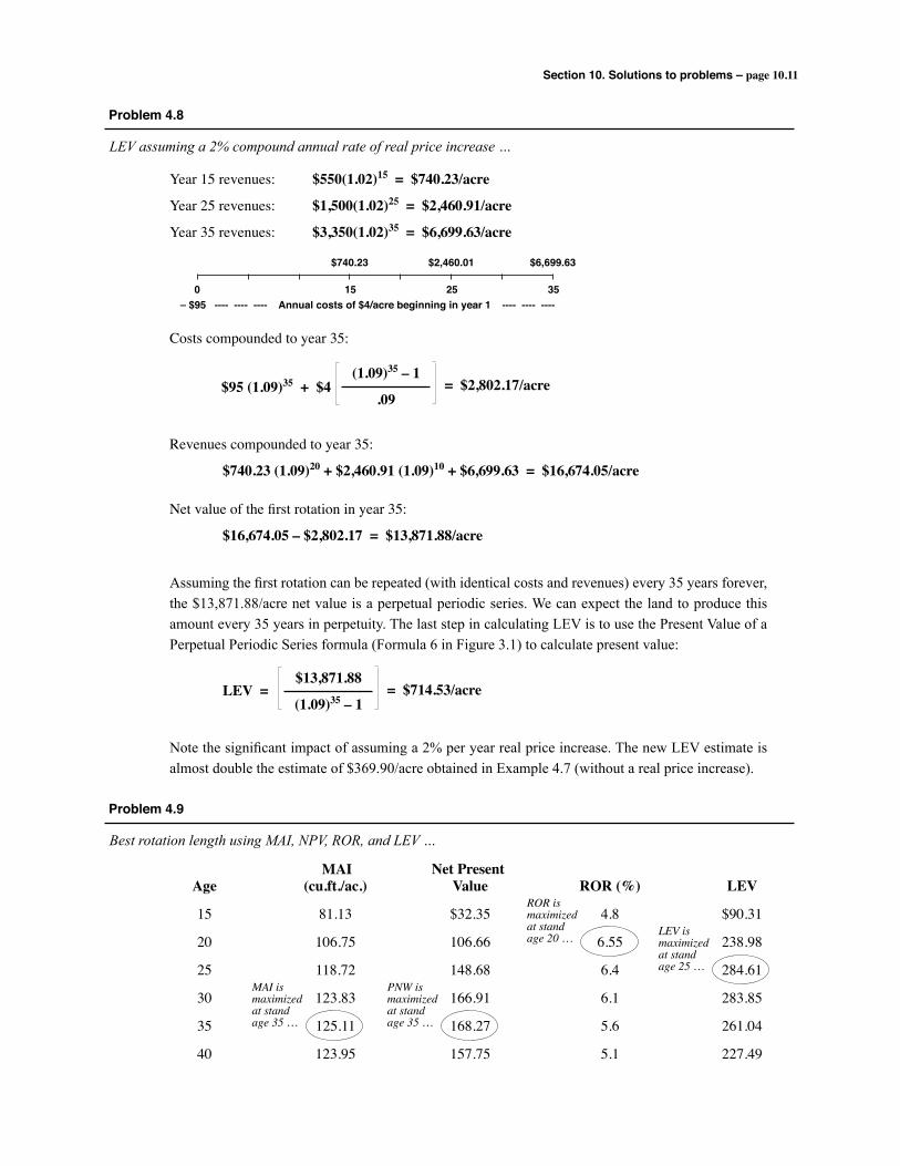
Section 10. Solutions to problems – page 10.11
Problem 4.8
LEV assuming a 2% compound annual rate of real price increase …
Year15revenues: $550(1.02)15 = $740.23/acre
Year25revenues: $1,500(1.02)25 = $2,460.91/acre
Year35revenues: $3,350(1.02)35 = $6,699.63/acre
Costscompoundedtoyear35:
Revenuescompoundedtoyear35:
$740.23 (1.09)20 + $2,460.91 (1.09)10 + $6,699.63 = $16,674.05/acre
Netvalueofthefirstrotationinyear35:
$16,674.05 – $2,802.17 = $13,871.88/acre
Assuming the first rotation can be repeated (with identical costs and revenues) every 35 years forever, the $13,871.88/acre net value is a perpetual periodic series. We can expect the land to produce this amount every 35 years in perpetuity. The last step in calculating LEV is to use the Present Value of a Perpetual Periodic Series formula (Formula 6 in Figure 3.1) to calculate present value:
Note the significant impact of assuming a 2% per year real price increase. The new LEV estimate is almost double the estimate of $369.90/acre obtained in Example 4.7 (without a real price increase).
= $2,802.17/acre(1.09)35 – 1
.09$95 (1.09)35 + $4
0 15 25 35
$740.23 $2,460.01 $6,699.63
– $95 ---- ---- ---- Annual costs of $4/acre beginning in year 1 ---- ---- ----
= $714.53/acre$13,871.88
(1.09)35 – 1LEV =
Problem 4.9
Best rotation length using MAI, NPV, ROR, and LEV …
Age
15
20
25
30
35
40
(cu.ft./ac.)
81.13
106.75
118.72
123.83
125.11
123.95
Value
$32.35
106.66
148.68
166.91
168.27
157.75
ROR (%)
4.8
6.55
6.4
6.1
5.6
5.1
LEV
$90.31
238.98
284.61
283.85
261.04
227.49
MAI ismaximizedat standage 35 …
PNW ismaximizedat standage 35 …
ROR ismaximizedat standage 20 … LEV is
maximizedat standage 25 …
MAI Net Present
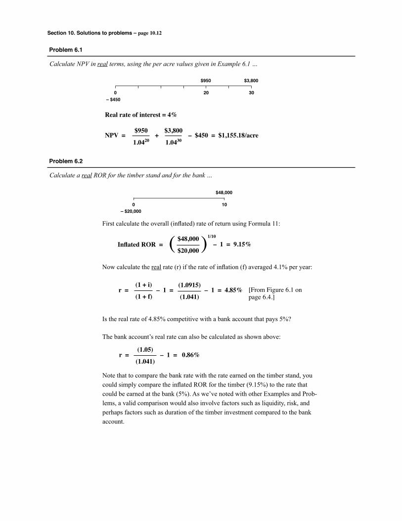
Section 10. Solutions to problems – page 10.12
Problem 6.1
Calculate NPV in real terms, using the per acre values given in Example 6.1 …
0 20 30
$950 $3,800
– $450
Real rate of interest = 4%
NPV = + – $450 = $1,155.18/acre$950
1.0420
$3,800
1.0430
Problem 6.2
Calculate a real ROR for the timber stand and for the bank …
0 10
$48,000
– $20,000
First calculate the overall (inflated) rate of return using Formula 11:
Now calculate the real rate (r) if the rate of inflation (f) averaged 4.1% per year:
Is the real rate of 4.85% competitive with a bank account that pays 5%?
The bank account’s real rate can also be calculated as shown above:
Inflated ROR =$48,000
$20,000( (1/10
– 1 = 9.15%
r = – 1 = – 1 = 4.85%(1 + i)
(1 + f)
(1.0915)
(1.041)[FromFigure6.1onpage6.4.]
r = – 1 = 0.86%(1.05)
(1.041)
Note that to compare the bank rate with the rate earned on the timber stand, youcould simply compare the inflated ROR for the timber (9.15%) to the rate that could be earned at the bank (5%). As we’ve noted with other Examples and Prob-lems, a valid comparison would also involve factors such as liquidity, risk, and perhaps factors such as duration of the timber investment compared to the bank account.
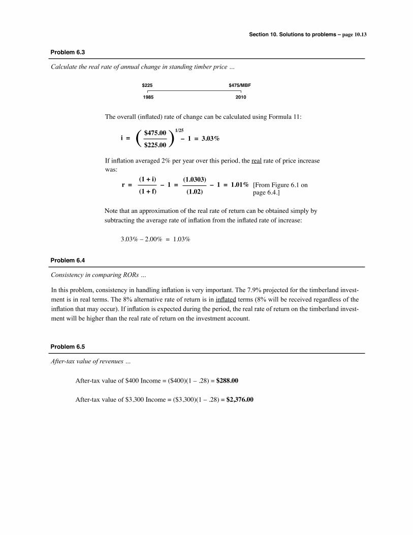
Section 10. Solutions to problems – page 10.13
Problem 6.3
Calculate the real rate of annual change in standing timber price …
1985 2010
$225 $475/MBF
Theoverall(inflated)rateofchangecanbecalculatedusingFormula11:
Ifinflationaveraged2%peryearoverthisperiod,therealrateofpriceincreasewas:
i =$475.00
$225.00( (1/25
– 1 = 3.03%
r = – 1 = – 1 = 1.01%(1 + i)
(1 + f)
(1.0303)
(1.02)
Notethatanapproximationoftherealrateofreturncanbeobtainedsimplybysubtractingtheaveragerateofinflationfromtheinflatedrateofincrease:
3.03%–2.00%=1.03%
[FromFigure6.1onpage6.4.]
Problem 6.4
Consistency in comparing RORs …
In this problem, consistency in handling inflation is very important. The 7.9% projected for the timberland invest-ment is in real terms. The 8% alternative rate of return is in inflated terms (8% will be received regardless of the inflation that may occur). If inflation is expected during the period, the real rate of return on the timberland invest-ment will be higher than the real rate of return on the investment account.
Problem 6.5
After-tax value of revenues …
After-taxvalueof$400Income=($400)(1–.28)=$288.00
After-taxvalueof$3,300Income=($3,300)(1–.28)=$2,376.00
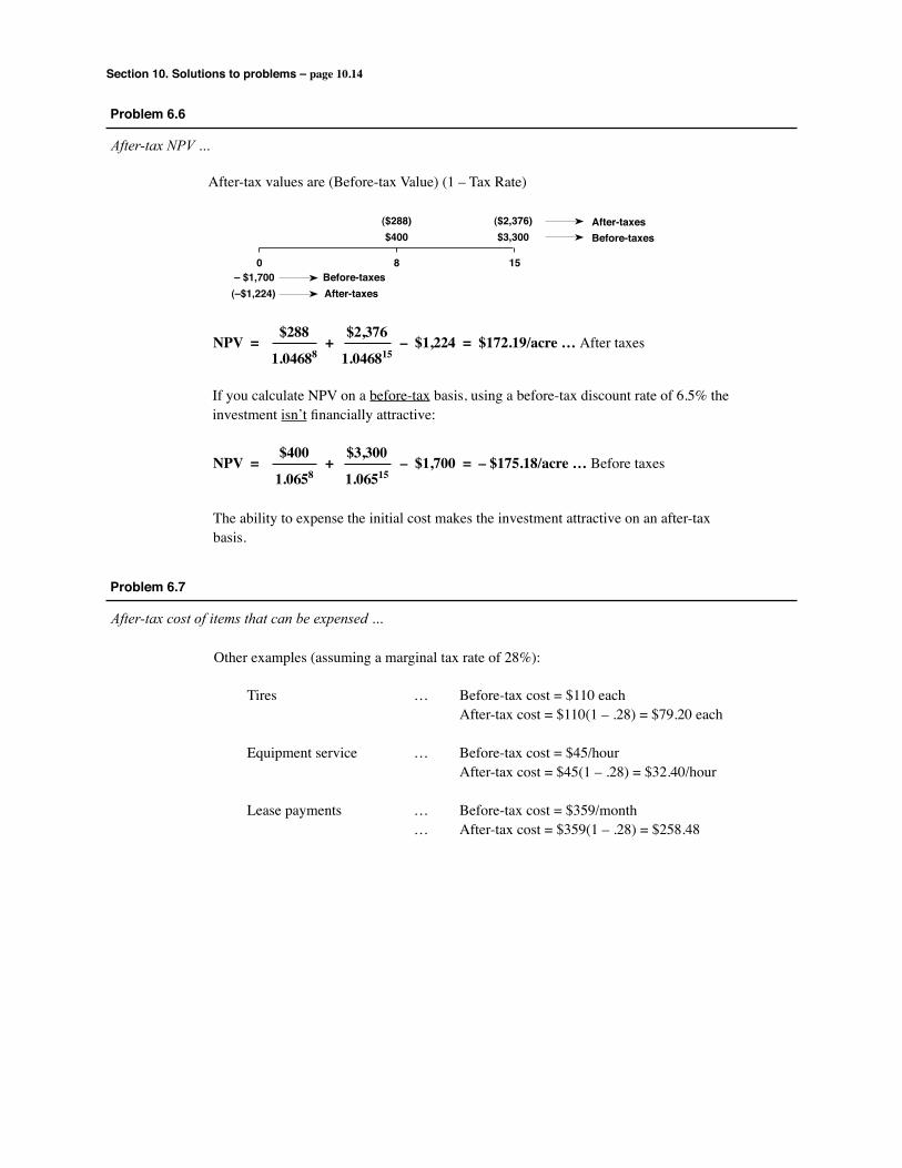
Section 10. Solutions to problems – page 10.14
Problem 6.6
After-tax NPV …
NPV = + – $1,224 = $172.19/acre … Aftertaxes$288
1.04688
$2,376
1.046815
0 8 15
($288) ($2,376) $400 $3,300
– $1,700 Before-taxes(–$1,224) After-taxes
Before-taxesAfter-taxes
After-taxvaluesare(Before-taxValue)(1–TaxRate)
IfyoucalculateNPVonabefore-taxbasis,usingabefore-taxdiscountrateof6.5%theinvestmentisn’tfinanciallyattractive:
NPV = + – $1,700 = – $175.18/acre … Beforetaxes$400
1.0658
$3,300
1.06515
Theabilitytoexpensetheinitialcostmakestheinvestmentattractiveonanafter-taxbasis.
Problem 6.7
After-tax cost of items that can be expensed …
Otherexamples(assumingamarginaltaxrateof28%):
Tires … Before-taxcost=$110each After-taxcost=$110(1–.28)=$79.20each
Equipmentservice … Before-taxcost=$45/hour After-taxcost=$45(1–.28)=$32.40/hour
Leasepayments … Before-taxcost=$359/month … After-taxcost=$359(1–.28)=$258.48
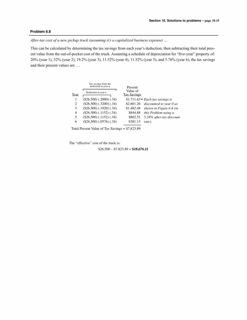
Section 10. Solutions to problems – page 10.15
What’s the after-tax cost of a skidder with a purchase price of $175,000? Assume the buyer is in a 34% marginal tax bracket. and uses an after-tax discount rate of 6% (after-tax discount rates are discussed in the next subsection).
Forthisexample,weapplythescheduleofdeductionsshownfor5-yearproperty(listedinthetextboxonpage6.16).Therearesixdeductions:
The“effective”costofthetruckis:
$26,500–$7,823.89=$18,676.11
Each tax savings is discounted to year 0 as shown in Figure 6.4 (in this Problem using a 5.28% after-tax discount rate).
1 ($26,500)(.2000)(.34) $1,711.632 ($26,500)(.3200)(.34) $2,601.263 ($26,500)(.1920)(.34) $1,482.484 ($26,500)(.1152)(.34) $844.885 ($26,500)(.1152)(.34) $802.516 ($26,500)(.0576)(.34) $381.13
YearDeductioninyearn
Taxsavingsfromthedeductioninyearn Present
ValueofTaxSavings
TotalPresentValueofTaxSavings=$7,823.89
Problem 6.8
After-tax cost of a new pickup truck (assuming it’s a capitalized business expense) …
This can be calculated by determining the tax savings from each year’s deduction, then subtracting their total pres-ent value from the out-of-pocket cost of the truck. Assuming a schedule of depreciation for “five-year” property of: 20% (year 1), 32% (year 2), 19.2% (year 3), 11.52% (year 4), 11.52% (year 5), and 5.76% (year 6), the tax savings and their present values are …

Section 10. Solutions to problems – page 10.16
Problem 7.1
LEV assuming lower site quality land …
There are many potential reasons for such differences. First, the market value of land is based on its potential returns, and there may be land uses that have a higher return than timber production. In this case, market transac-tions may produce prices that are much higher than timber-based LEV estimates. Even if the land remains in timber production, the estimated LEV for one person or firm isn’t likely to be the same as the value you’d calculate for another person or firm; there are many possible assumptions about yields, management, prices, and costs, as well as the choice of a discount rate. Also, the sale price for a specific tract of timberland may be higher than LEV simply because a particular buyer had non-monetary and/or strategic reasons for wanting to own a particular tract.
Another potential reason for differences between calculated LEVs and market transaction prices is lack of perfect information. Buyers and sellers in the market don’t always have good information about potential timberland (or other) investments. There can also be a lag between fundamental changes in supply and demand for timber, and the bid prices for bare land. For example, if timber prices increase dramatically in a short period of time (say five years), and the timber prices are expected to remain high in the long term, market prices for bare land can be sig-nificantly lower than what you calculate as an LEV. In such cases, market transactions don’t reflect the new, higher values for timber production.
Diagram
Calculate
Interpret
18
$300
30
$2,100
0 25
$600
– $120 – Annual costs of $5/acre beginning in year 1 –
Costscompoundedtoyear30:
Revenuescompoundedtoyear30:
$300(1.06)12 + $600(1.06)5 + $2,100 = $3,506.59/acre
Netvalueofthefirstrotationinyear30:
$3,506.59 – $1,804.51 = $2,422.08/acre
Assuming the first rotation can be repeated (with identical costs and revenues) every 30 years forever, the $2,422.08/acre net value is a perpetual periodic series. We can expect the land to produce this amount every 30 years in perpetuity. The last step in calculating LEV is to use the Present Value of a Perpetual Periodic Series formula (Formula 6 in Figure 3.1) to calculate Present Value:
Given the assumptions above, the lower site quality inherited land has a value of $510.61/acre for timber production. This value is based on many assumptions, and a different estimated valuewillbeobtainedifanyofthemarechanged.
(1.06)30 – 1.06
$120(1.06)30 + $5 = $1,084.51/acre
$2,422.08(1.06)30 – 1
LEV = = $510.61/acre
Why do land prices observed in market transactions differ from what you calculate as an LEV?
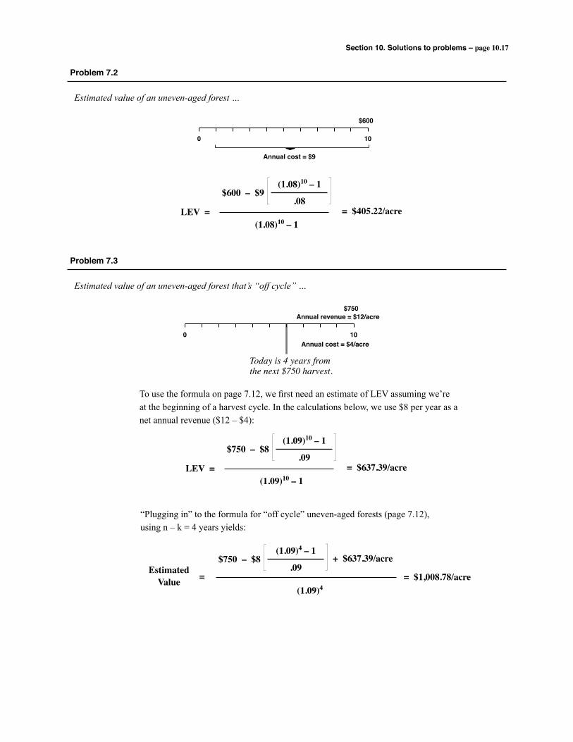
Section 10. Solutions to problems – page 10.17
(1.09)4 – 1
.09
“Plugging in” to the formula for “off cycle” uneven-aged forests (page 7.12),using n – k = 4 years yields:
$750 – $8
$750 – $8
$600 – $9
Problem 7.2
Estimated value of an uneven-aged forest …
0 10
$600
Annual cost = $9
LEV = = $405.22/acre
(1.08)10 – 1
.08
(1.08)10 – 1
Problem 7.3
Estimated value of an uneven-aged forest that’s “off cycle” …
0 10
$750
Annual cost = $4/acre
Annual revenue = $12/acre
Today is 4 years fromthe next $750 harvest.
To use the formula on page 7.12, we first need an estimate of LEV assuming we’re at the beginning of a harvest cycle. In the calculations below, we use $8 per year as a net annual revenue ($12 – $4):
LEV = = $637.39/acre
(1.09)10 – 1
.09
(1.09)10 – 1
EstimatedValue = $1,008.78/acre
(1.09)4
+ $637.39/acre
=

Index
accept/reject investment decisions 4.11, 4.14 4.23–4.28, 4.47adjusted basis (for depletion) 6.15, 9.26–9.29after-tax discount rate 6.17, 6.19, 6.22, 6.28after-tax costs 6.12–6.21, 6.27–6.28, 9.34agricultural land use 4.30alternative rate of return 2.13, 2.16, 5.14amortization 6.20, 9.34annual equivalent 4.4annual income equivalent 4.4Austrian formula 9.67Bare Land Value 4.18basal area 9.49–9.51basis for depletion 6.14–6.15, 9.26–9.29Benefit/Cost ratio (B/C) 4.8–4.9, 4.26, 8.3buyer’s value 7.17capital budgeting 4.23, 4.38, 4.47capital gains income 6.10, 9.25capital recovery 3.23capitalization 9.26capitalized costs 6.14, 6.28, 9.26cash-flow diagram 2.14, 2.16, 3.1, 3.4, 3.12, 3.16–3.17constant dollars 6.2comparable sales 7.6Composite Rate of Return 4.16, 4.23, 4.26compounding 1.8, 2.4, 2.13–2.14computer programs 8.1–8.6Consumer Price Index (CPI) 6.3cost-less depreciation 7.6cost of capital 2.13, 2.16, 5.14cottonwood 4.30credits (income tax credits) 6.20–6.21Crown Competition Factor 9.54–9.55current dollars 6.2cutting cycle 4.18–4.19, 7.7–7.13decision tree diagram 3.2, 3.4, 3.9, 3.15, 3.23, 3.29, 3.37–3.40deductions (income tax deductions) 6.14density (measures of stand density) 9.49–9.70depletion account 6.14–6.15, 9.29depletion rate 6.14–6.15, 9.29depreciation 6.16–6.17discount rate (see also interest rate) 4.37, 5.5 5.13–5.18, 6.22 … for public agencies 5.15 … for corporations 5.15 … for private individuals 5.15
discounting 2.4, 2.13–2.14effective cost 6.17, 6.19–6.21effective interest rate 9.19end-of-year assumption 2.14, 2.16, 3.27, 3.37equal annual equivalent 4.4equipment 3.20, 3.24–3.25, 3.28, 3.36, 4.35, 5.3, 6.16–6.19, 9.27equivalence 1.7, 2.13equivalent 1.5, 1.8, 1.12, 2.13, 3.6equivalent acres 9.69–9.70Equivalent Annual Income (EAI) 1.5, 4.4–4.7, 4.9, 4.22–4.23, 4.26, 4.28–4.31, 8.3even-aged stand valuation 7.3–7.6, 7.22exception rate 5.14expensed costs 6.12, 6.28, 9.26exponent (exponentiation, exponential) 1.10, 1.12fair market value 9.27Faustmann formula (see Land Expectation Value)fertilization 2.6, 2.8, 3.22, 4.23financial maturity 1.2, 2.5, 4.34, 5.13, 9.6FORVAL 8.1–8.6Future Value 1.9, 2.2, 2.13, 2.16, 3.3, 3.5, 3.6Future Value of a Single Sum 3.3Future Value of a Terminating Annual Series 3.6, 9.8generalizations 1.3, 1.12growing stock 9.62–9.63guiding rate of return 2.13, 2.16, 5.14Hanzlik’s formula 9.69hardwood 2.9, 3.12, 3.16, 4.25harvest scheduling 9.71herbicides 2.6, 2.8, 5.3history of interest rates 1.11Hundeshagen’s formula` 6.65hurdle rate 2.13, 2.16, 5.14immature timber valuation 7.16–7.21, 7.24, 8.3income capitalization 7.3, 7.6income taxes 6.10–6.28, 9.25incremental analysis 5.2, 5.19inflation 6.1–6.9, 6.26, 9.24Internal Rate of Return (see Rate of Return)interest rate (see also discount rate) 2.13, 2.16, 5.5, 5.7, 5.14installments 3.23, 8.6–8.7, 9.17–9.18iterative process 4.10, 4.12land account 6.14, 9.27land use alternatives 4.30, 4.34, 4.47Land Expectation Value (LEV) 4.4, 4.18–4.23, 4.26, 4.28–4.31, 4.42≠4.44, 5.13, 7.3–7.13
Index
lease 1.2, 3.7, 3.19, 4.7, 4.13liquidation value of timber 7.14–7.15, 7.23logging 3.20, 3.24marginal analysis 2.6, 5.2, 5.19marketing 7.24–7.25mean annual increment 4.40–4.43, 9.45Meyer’s amortization formula 9.68mortgage 1.4, 3.35mutually exclusive 4.29, 4.35–4.36, 4.40, 4.47net annual equivalent 4.4Net Present Value (NPV) 3.1, 3.10, 4.2–4.4, 4.6, 4.9, 4.18, 4.26–4.31, 4.41–4.44nominal (vs. real) 5.16, 6.2non-annual compounding 3.27, 3.33–3.34, 9.18–9.19normal forest 9.59off-cycle uneven-aged stands 7.11–7.13opportunity costs 5.11–5.14, 5.19, 7.18–7.19, 9.7ordinary income 9.25original cost basis 9.26–9.27Paulownia 2.10Payback Period 4.17, 4.23, 4.26payments 3.2–3.37, 8.3, 9.17–9.18percent 1.11periodic annual increment 9.45–9.47power of compound interest 1.9–1.10, 1.12practice test on forest valuation 9.39–9.44practice test on forest management 9.81–9.105precommercial timber valuation (see immature timber valuation)Present Value 1.9, 2.2, 2.13, 2.16Present Value of a Perpetual Annual Series 3.13, 9.8Present Value of a Perpetual Periodic Series 3.14Present Value of a Single Sum 3.5Present Value of a Terminating Annual Series 3.8prices (see stumpage prices)principal 1.6–1.8property taxes 3.19pruning 2.6, 5.2pulpwood vs. sawtimber 4.32ranking investments 4.14, 4.23, 4.27–4.38, 4.47Rate of Return (ROR) 2.5, 4.10–4.14, 4.26–4.28, 4.42–4.44, 8.3real (vs. nominal) 5.16, 6.2real estate 3.36, 7.6real price increase 4.19, 4.21, 6.7Realizable Rate of Return (see Composite ROR)
reforestation tax incentives 6.20–6.21Registered Forester exam 9.1–9.105regulated forest 9.59–9.70reinvestment assumption 4.27relative density 9.53relative spacing 9.55–9.56Return on Investment (ROI) (see Rate of Return)risk and uncertainty 2.9, 5.4–5.10, 5.19rotation age 4.19, 4.32, 4.40–4.44, 5.6, 9.6Rule of 72 4.15seller’s value 7.17sensitivity analysis 2.9, 2.15, 3.23–3.26, 3.28, 3.32, 9.17–9.18sinking fund 3.24–3.25, 3.28site index 9.58site preparation 5.6software (see computer programs)Soil Expectation Value (see Land Expectation Value)stand density index 9.51–9.52stumpage prices (and stumpage value) 2.9, 3.22, 4.21, 5.6–5.7, 6.7–6.8, 7.15, 8.6 (residual aspects of stumpage 7.14)sunk costs 5.3, 5.19taxes (see property taxes and/or income taxes)Terminating Periodic Series 9.11–9.14timber account 6.14–6.15, 9.26timber prices (see stumpage prices)timber value growth percent 9.6time value of money 1.1, 1.5, 1.12transactions evidence 7.6uncertainty (see risk and uncertainty)uneven-aged stand valuation 7.7–7.13, 7.22–7.23valuation 4.19, 4.23, 4.39, 7.1–7.26 … of timberland 7.3–7.13 … of standing timber 7.14–7.21, 7.23–7.24Von Mantel’s formula 9.66–9.67wildlife 1.2, 4.3, 4.7
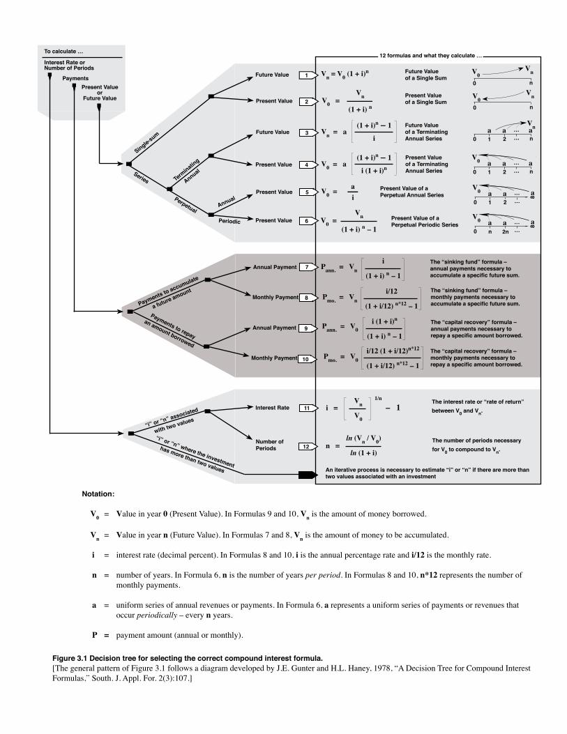
Vn = V0 (1 + i)n
V0 = Vn
(1 + i) n
Future Valueof a Single Sum
Present Valueof a Single Sum
V0Vn
0 n
V0Vn
0 n
Future Valueof a TerminatingAnnual Series
Vn = a(1 + i)n – 1
i
Vn
0 n1 2 …a a … a
Present Valueof a TerminatingAnnual Series
V0 = a(1 + i)n – 1
i (1 + i)n
V0
0 n1 2 …a a … a
V0 = ai
Present Value of aPerpetual Annual Series
V0
0
8
1 2 …a a … a
12 formulas and what they calculate …
1
2
3
4
5
6 V0 = Vn
(1 + i) n – 1Present Value of a Perpetual Periodic Series
V0
0
8
n 2n …a a … a
Future Value
Present Value
Future Value
Present Value
Present Value
Present Value
Annual
Periodic
Perpetual
Terminatin
g
AnnualSeries
Single-sum
Present Valueor
Future Value
Payments
To calculate …
Interest Rate orNumber of Periods
7 Pann. = Vn The “sinking fund” formula –annual payments necessary toaccumulate a specific future sum.
Annual Paymenti
(1 + i) n – 1
8The “sinking fund” formula –monthly payments necessary toaccumulate a specific future sum.
Monthly Payment Pmo. = Vn i/12
(1 + i/12) n*12 – 1
9Annual Payment
10Monthly Payment
Pann. = V0 i (1 + i)n
(1 + i) n – 1
Pmo. = V0 i/12 (1 + i/12)n*12
(1 + i/12) n*12 – 1
Payments to repay
an amount borrowed
The “capital recovery” formula –annual payments necessary torepay a specific amount borrowed.
The “capital recovery” formula –monthly payments necessary torepay a specific amount borrowed.
Payments to accumulate
a future amount
12Number ofPeriods n =
ln (Vn / V0)
ln (1 + i)
The number of periods necessaryfor V0 to compound to Vn.
“i” or “n” where the investment
has more than two values
“i” or “n” associated
with two values
Interest RateThe interest rate or “rate of return”between V0 and Vn.i = – 1
Vn
V0
1/n
11
An iterative process is necessary to estimate “i” or “n” if there are more thantwo values associated with an investment
Notation:
V0 = Value in year 0 (Present Value). In Formulas 9 and 10, Vn is the amount of money borrowed.
Vn = Value in year n (Future Value). In Formulas 7 and 8, Vn is the amount of money to be accumulated.
i = interest rate (decimal percent). In Formulas 8 and 10, i is the annual percentage rate and i/12 is the monthly rate.
n = number of years. In Formula 6, n is the number of years per period. In Formulas 8 and 10, n*12 represents the number of monthly payments.
a = uniform series of annual revenues or payments. In Formula 6, a represents a uniform series of payments or revenues that occur periodically – every n years.
P = payment amount (annual or monthly).
Figure 3.1 Decision tree for selecting the correct compound interest formula.[The general pattern of Figure 3.1 follows a diagram developed by J.E. Gunter and H.L. Haney, 1978, “A Decision Tree for Compound Interest Formulas,” South. J. Appl. For. 2(3):107.]

Steps in Forestry Investment Analysis
Account for the time value of the cash flows on the cash-flow diagram. You can do this by using the formulas on page 3.39 (repeated on the last page of the book for convenience), or by using a financial calculator, or by using a specialized computer program. The type of compounding and discounting depends on the type of analysis you’re doing, the specific criteria you’re calculating, etc., but in all cases the analysis should be consistent with respect to taxes and inflation:
After calculating NPV or other criteria, consider the sensitivity of your results to some of the input assumptions. When you change the assumed values in the analysis, does the acceptability of the investment change? If you’re ranking investments, does the ranking change? In forestry, the discount rate and the stumpage prices assumed are often very important to analysis results. (Sensitivity analysis is discussed in Section 5, beginning on page 5.4.)
This diagram refers to page numbers and discussion in: Basic Concepts in Forest Valuation and Investment Analysis by S.H. Bullard and T.J. Straka (2011).
Financial criteria and what they should be used for …
NPV – Net Present Value is the present value of all revenues minus the present value of all costs. NPV can be used for accept/reject investment decisions, and is highly preferred for ranking investments. (NPV discussion begins on page 4.2.)
EAI – Equivalent Annual Income is the NPV for an investment expressed as an “annual equivalent.” It can be used to rank invest-ments of different length. (EAI discussion begins on page 4.4.) To calculate EAI, use formula 9 in the decision tree diagram on page 3.39, with NPV as the “amount borrowed,” and the length of the investment as “n.”
B/C Ratio – Benefit/Cost Ratio is the present value of all revenues divided by the present value of all costs. B/C is used for accept/reject decisions by some U.S. government agencies. (B/C discussion begins on page 4.8.)
ROR – The Rate of Return of an investment is the average compound rate of capital appreciation. It’s the interest rate that makes the present value of the revenues and the present value of the costs equal. The criterion is widely used for accept/reject deci-sions, but it should not be used to rank investments. For ranking, NPV (or a form of NPV like EAI or LEV) is recommended. (Discussion of ROR begins on page 4.10.)
LEV – Land Expectation Value is a special case of NPV. LEV is the net present value of an infinite series of identical even-aged stands of timber, or an infinite series of periodic harvests under uneven-aged management. LEV is an estimate of the value of bare land for growing timber, so it’s sometimes called Bare Land Value or Soil Expectation Value. LEV is calculated by com-pounding costs and revenues associated with the first rotation or cutting cycle to the end of the period, and then discounting this net future value to the present using the formula for the Present Value of a Perpetual Periodic Series … formula 6 on page 3.39. (LEV discussion begins on page 4.18.)
What discount rate should you use? The interest rate is extremely important. The appropriate rate depends on several factors – see Section 5.6 Choosing a discount rate (page 5.14). As stated above, it’s critical that the discount rate be consistent with all costs and revenues in terms of whether taxes and inflation are included or excluded.
Make sure that the discount rate and all costs and revenues are either in before-tax terms or in after-tax terms, and that they are also consistent in including or excluding inflation.
Consistency is critical, whether you’re using a computer program or a calcu-lator, and regardless of which financial criterion or criteria you’re calculating.
There are four potential combinations: 1. After-Taxes, With Inflation 2. Before-Taxes, With Inflation 3. Before-Taxes, Without Inflation 4. After-Taxes, Without Inflation
– $400 Place Costs Below the Time - line
Place Revenues Above the Time- line $1,000
0 1 2 3
4 Cheat Sheet
3. Calculate and interpret financial criteria:
4. Consider the need for sensitivity analysis:
2. Do the compounding and discounting:
1. Start with a cash-flow diagram:
Related Documents