Basic Algorithms and Combinatorics in Computational Geometry* 1

Basic Algorithms and Combinatorics in

Computational Geometry�

Leonidas Guibas

Graphics Laboratory

Computer Science Department

Stanford University

Stanford� CA �����

guibas�cs�stanford�edu

� Introduction

Computational geometry is� in its broadest sense� the study of geometric problemsfrom a computational point of view� At the core of the �eld is a set of techniques forthe design and analysis of geometric algorithms� These algorithms often operate on�and are guided by� a set of data structures that are ubiquitous in geometric computing�These include arrangements� Voronoi diagrams� and Delaunay triangulations� It isthe purpose of this paper to present a tutorial introduction to these basic geometricdata structures�

The material for this paper is assembled from lectures that the author has given inhis computational geometry courses at the Massachusetts Institute of Technology andat Stanford University over the past four years� The lectures were scribed by studentsand then revised by the author� A list of the students who contributed their notesappears at the end of the paper� Additional material on the data structures presentedhere can be found in the standard texts Computational Geometry� An Introduction�by F� P� Preparata and M� I� Shamos �Springer�Verlag� ����� and Algorithms inCombinatorial Geometry by H� Edelsbrunner �Springer�Verlag� ���� as well as inthe additional references at the end of the paper�

�This work by Leonidas Guibas has been supported by grants from Digital Equipment� Toshiba�and Mitsubishi Corporations�

�

Let us end this brief introduction by noting that the excitement of computa�tional geometry is due to a combination of factors� deep connections with classicalmathematics and theoretical computer science on the one hand� and many ties withapplications on the other� Indeed� the origins of the discipline clearly lie in geo�metric questions that arose in areas such as computer graphics and solid modeling�computer�aided design� robotics� computer vision� etc� Not only have these moreapplied areas been a source of problems and inspiration for computational geometrybut� conversely� several techniques from computational geometry have been founduseful in practice as well� The level of mathematical sophistication needed for workin the �eld has risen sharply in the last four to �ve years� Nevertheless� many of thenew algorithms are simple and practical to implement�it is only their analysis thatrequires advanced mathematical tools�

Because of the tutorial nature of this write�up� few references are given in themain body of the text� The papers on which this exposition is based are listed in thebibliography section at the end�

� Arrangements of Lines in the Plane

Computation Model

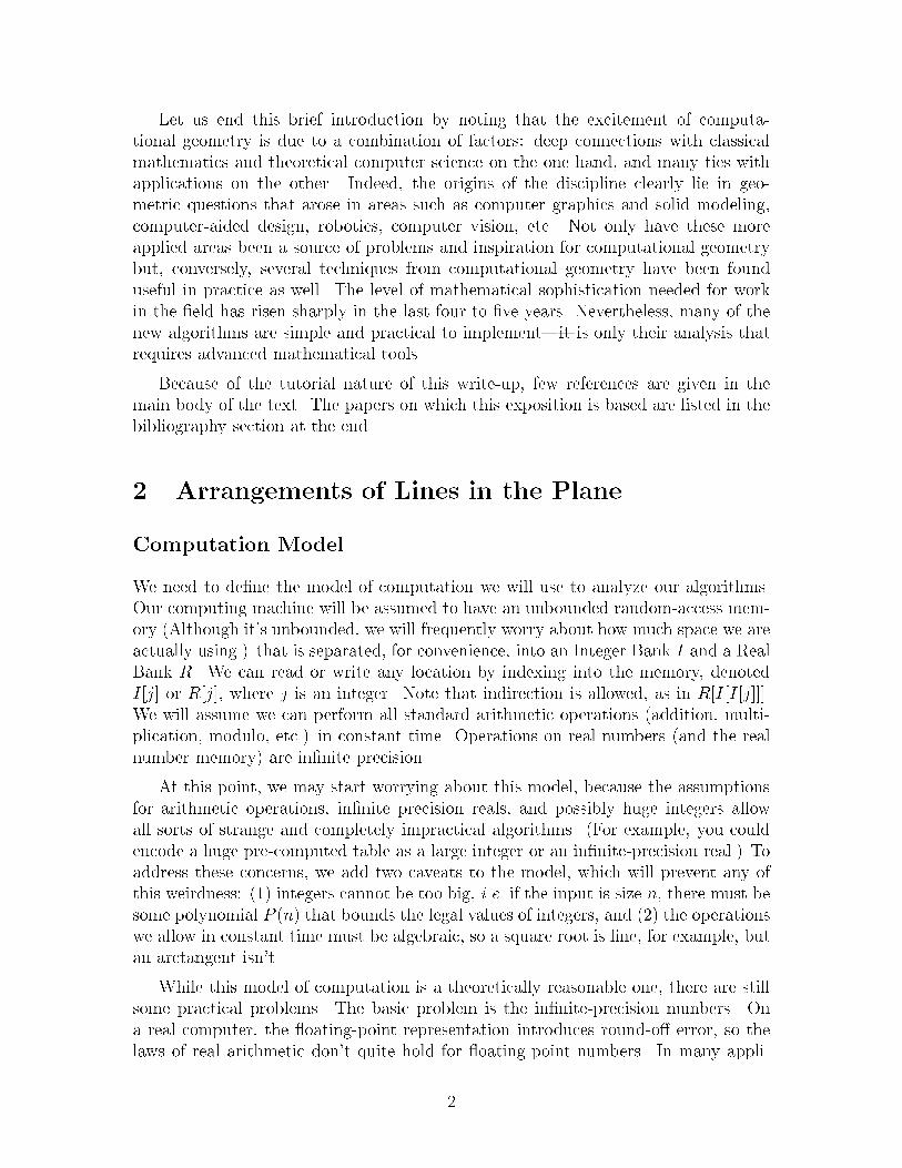
We need to de�ne the model of computation we will use to analyze our algorithms�Our computing machine will be assumed to have an unbounded random�access mem�ory �Although it s unbounded� we will frequently worry about how much space we areactually using� that is separated� for convenience� into an Integer Bank I and a RealBank R� We can read or write any location by indexing into the memory� denotedI�j� or R�j�� where j is an integer� Note that indirection is allowed� as in R�I�I�j����We will assume we can perform all standard arithmetic operations �addition� multi�plication� modulo� etc� in constant time� Operations on real numbers �and the realnumber memory are in�nite precision�

At this point� we may start worrying about this model� because the assumptionsfor arithmetic operations� in�nite precision reals� and possibly huge integers allowall sorts of strange and completely impractical algorithms� �For example� you couldencode a huge pre�computed table as a large integer or an in�nite�precision real� Toaddress these concerns� we add two caveats to the model� which will prevent any ofthis weirdness� �� integers cannot be too big� i�e� if the input is size n� there must besome polynomial P �n that bounds the legal values of integers� and �� the operationswe allow in constant time must be algebraic� so a square root is �ne� for example� butan arctangent isn t�

While this model of computation is a theoretically reasonable one� there are stillsome practical problems� The basic problem is the in�nite�precision numbers� Ona real computer� the �oating�point representation introduces round�o� error� so thelaws of real arithmetic don t quite hold for �oating�point numbers� In many appli�

�

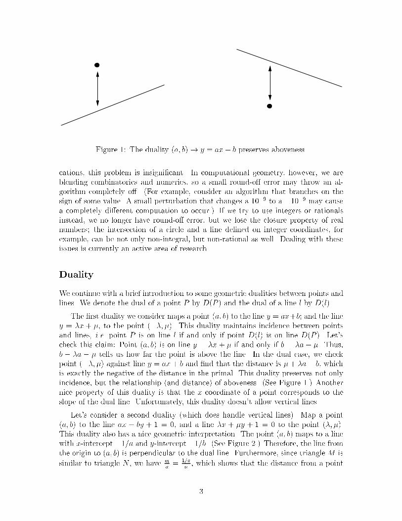
Figure �� The duality �a� b �� y � ax � b preserves aboveness�

cations� this problem is insigni�cant� In computational geometry� however� we areblending combinatorics and numerics� so a small round�o� error may throw an al�gorithm completely o�� �For example� consider an algorithm that branches on thesign of some value� A small perturbation that changes a ���� to a ����� may causea completely di�erent computation to occur� If we try to use integers or rationalsinstead� we no longer have round�o� error� but we lose the closure property of realnumbers� the intersection of a circle and a line de�ned on integer coordinates� forexample� can be not only non�integral� but non�rational as well� Dealing with theseissues is currently an active area of research�

Duality

We continue with a brief introduction to some geometric dualities between points andlines� We denote the dual of a point P by D�P and the dual of a line l by D�l�

The �rst duality we consider maps a point �a� b to the line y � ax�b� and the liney � �x � �� to the point ���� �� This duality maintains incidence between pointsand lines� i�e� point P is on line l if and only if point D�l is on line D�P � Let scheck this claim� Point �a� b is on line y � �x � � if and only if b � �a � �� Thus�b � �a � � tells us how far the point is above the line� In the dual case� we checkpoint ���� � against line y � ax � b and �nd that the distance is � � �a� b� whichis exactly the negative of the distance in the primal� This duality preserves not onlyincidence� but the relationship �and distance of aboveness� �See Figure �� Anothernice property of this duality is that the x coordinate of a point corresponds to theslope of the dual line� Unfortunately� this duality doesn t allow vertical lines�

Let s consider a second duality �which does handle vertical lines� Map a point�a� b to the line ax � by � � � �� and a line �x � �y � � � � to the point ��� ��This duality also has a nice geometric interpretation� The point �a� b maps to a linewith x�intercept ���a and y�intercept ���b� �See Figure �� Therefore� the line fromthe origin to �a� b is perpendicular to the dual line� Furthermore� since triangle M is

similar to triangle N � we have ma

� ��an

� which shows that the distance from a point

�

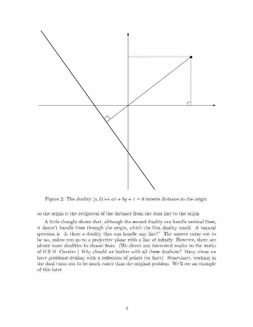
Figure �� The duality �a� b �� ax � by � � � � inverts distance to the origin�

to the origin is the reciprocal of the distance from the dual line to the origin�

A little thought shows that� although the second duality can handle vertical lines�it doesn t handle lines through the origin� which the �rst duality could� A naturalquestion is �Is there a duality that can handle any line�� The answer turns out tobe no� unless you go to a projective plane with a line at in�nity� However� there areplenty more dualities to choose from� �We direct any interested reader to the worksof H�S�M� Coxeter� Why should we bother with all these dualities� Many times wehave problems dealing with a collection of points �or lines� Sometimes� working inthe dual turns out to be much easier than the original problem� We ll see an exampleof this later�

�

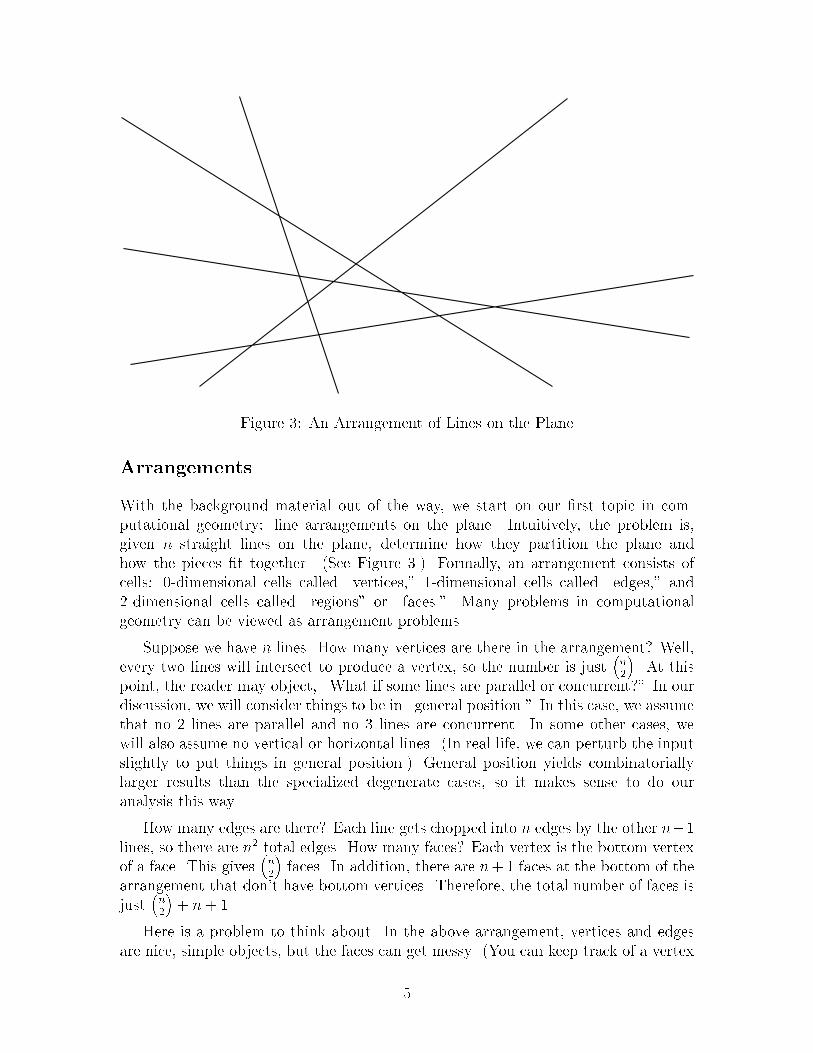
Figure �� An Arrangement of Lines on the Plane

Arrangements

With the background material out of the way� we start on our �rst topic in com�putational geometry� line arrangements on the plane� Intuitively� the problem is�given n straight lines on the plane� determine how they partition the plane andhow the pieces �t together� �See Figure �� Formally� an arrangement consists ofcells� ��dimensional cells called �vertices�� ��dimensional cells called �edges�� and��dimensional cells called �regions� or �faces�� Many problems in computationalgeometry can be viewed as arrangement problems�

Suppose we have n lines� How many vertices are there in the arrangement� Well�every two lines will intersect to produce a vertex� so the number is just

�n�

�� At this

point� the reader may object� �What if some lines are parallel or concurrent�� In ourdiscussion� we will consider things to be in �general position�� In this case� we assumethat no � lines are parallel and no � lines are concurrent� In some other cases� wewill also assume no vertical or horizontal lines� �In real life� we can perturb the inputslightly to put things in general position� General position yields combinatoriallylarger results than the specialized degenerate cases� so it makes sense to do ouranalysis this way�

How many edges are there� Each line gets chopped into n edges by the other n��lines� so there are n� total edges� How many faces� Each vertex is the bottom vertexof a face� This gives

�n�

�faces� In addition� there are n� � faces at the bottom of the

arrangement that don t have bottom vertices� Therefore� the total number of faces isjust

�n�

�� n � ��

Here is a problem to think about� In the above arrangement� vertices and edgesare nice� simple objects� but the faces can get messy� �You can keep track of a vertex

�

Figure �� Extending �threads� from each vertex triangulates an arrangement�

as just a pair of coordinates and an edge as just a pair of vertices� but you mayneed up to n edges to de�ne a face� In many applications� we want to have facesof bounded complexity� This modi�cation is called a �triangulated arrangement��One way to produce a triangulated arrangement is to take a normal arrangement andextend a �thread� up and down from each vertex until it hits a line� �See Figure ��Now� each face is a trapezoid� which only needs � edges to describe� �One might betempted to call what we just did �trapezoidalization� as opposed to �triangulation��In general� we ll use �triangulation� to refer to any scheme to reduce the faces to�nite complexity� The question is� �How many trapezoids do you get��

More Counting

The correct solution is ��n�

�� n � �� We arrive at this result by noting that each

thread breaks an existing face into two and that each vertex produces two threads�giving �

�n�

���n�

�� n � ��

Returning to the original �non�triangulated problem� we note that a face canhave as few as � and as many as n edges� How many edges does an average face have�Each edge counts toward both faces that it touches� so we have twice the number ofedges divided by the number of faces or �n���

�n�

�� n� �� which is approximately ��

Now� suppose we add a new line to the arrangement of n lines� What faces of theoriginal arrangement do we touch� These faces are called the �zone� or the �horizon�of the new line� �See Figure �� Let s do some more counting� How many faces arethere in a zone� Since we can intersect each of the original lines exactly once� andeach time we do this� we touch exactly one new face� there are n� � faces in the zone

�

Figure �� The zone of the darker line consists of the marked faces�

of a line�

A harder problem is counting the number of edges �or vertices in a zone� Wecan get a quick upper bound by noting that each face can have at most n edges� andthere are n � � faces in the zone� yielding an O�n� upper bound� Since the averagenumber of edges per face is � and the number of faces is n � �� we might wishfullyhope to get a linear bound� This argument� however� isn t logically valid since theaverage we computed was over all faces� so a given line might just run into the badones� A careful argument� though� does give us a linear bound� This argument is theZone Theorem�

The Zone Theorem

We re actually only dealing with the Zone Theorem �also known as the Horizon The�orem for lines on the plane� The Zone Theorem states�

Theorem �� The zone of a straight line intersecting an arrangement of n straightlines in the plane has at most �n edges� The same bound holds for the number ofvertices as well�

Proof� Without loss of generality� we can assume the new line is horizontal� �If not�we can always rotate our head slightly until it is� Let s only count the right edges ofthe faces of the zone� �Remember we re in general position� so every edge of a face iseither a right edge or a left edge� If we can bound the number of right edges by �n�we can then stand on our heads and apply the same argument to get the left edges�Combining the two counts will give us the desired �n bound�

Figure �� Introducing the dashed line creates the � additional marked edges�

Suppose we introduce the n lines of the arrangement one�at�a�time� ordered fromright to left by the intersection point of the line with the zone line� Each time weintroduce an additional line� we can create at most � new right edges� since the newline introduces one new right edge and splits two previous ones� �See Figure �� Aboveand below the intersection points� the already�added lines shield the new line fromhaving any further e�ect on the zone� Thus� we have the �n bound on right edges�QED

�We mention that applying this argument even more carefully gives a bound of�n� �� and that an even more precise argument gives a slightly lower bound� about���n�

So� we have the Zone Theorem� Who cares� Well� we can use the Zone Theoremto create an e�cient incremental method of computing arrangements� Suppose wehave an arrangement �like Figure � and we want to add an additional line �like thedark one in Figure �� we can compute the new arrangement by putting our left handon the wall of the zone and walking around the zone� marking o� faces whenever wecross the new line� �See Figure � �This is called a �labyrinth� walk� since you canget out of certain kinds of mazes this way� By the Zone Theorem� the cost of thiswalk is linear� Thus� we can add a line to an arrangement in linear time� yieldingan O�n� incremental algorithm to construct an arrangement� which is optimal upto a constant factor� This example nicely illustrates an application of combinatorialgeometry �the Zone Theorem to computational geometry �the incremental method�

�

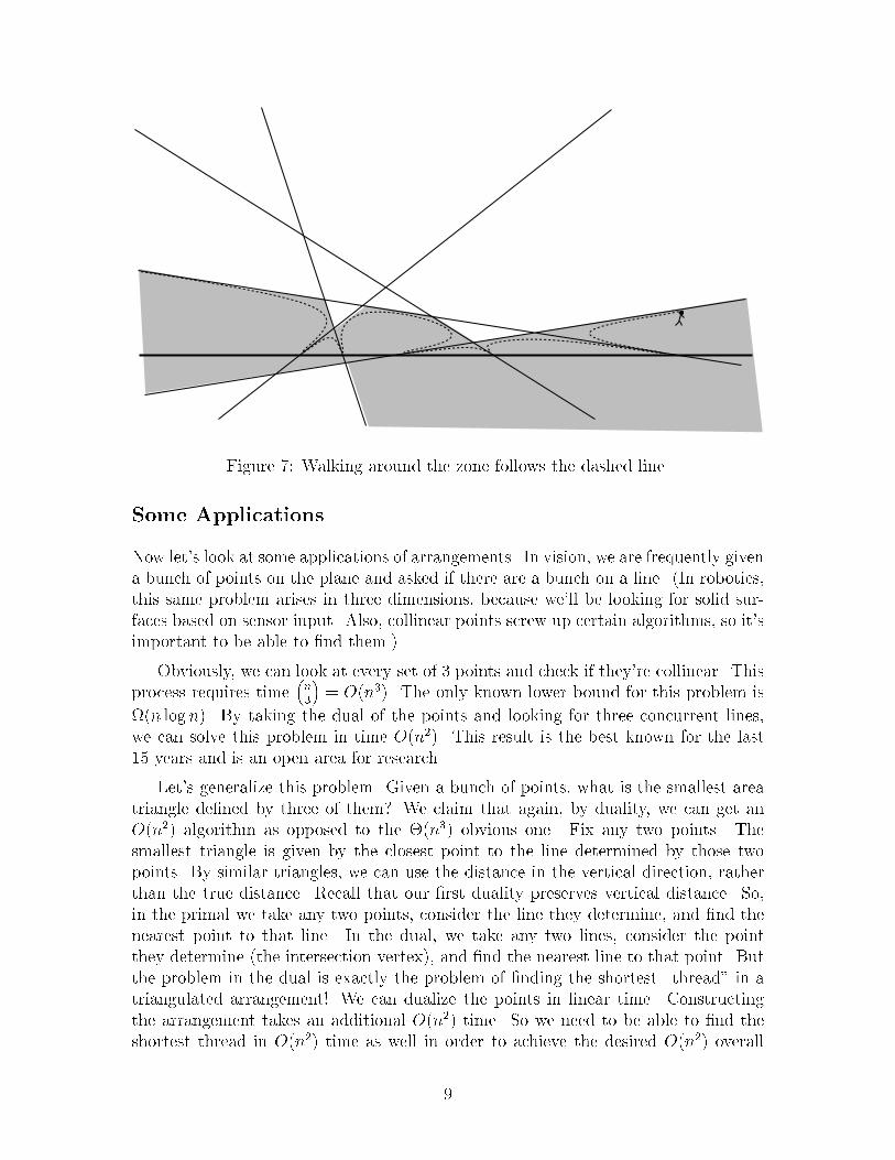
Figure � Walking around the zone follows the dashed line�

Some Applications

Now let s look at some applications of arrangements� In vision� we are frequently givena bunch of points on the plane and asked if there are a bunch on a line� �In robotics�this same problem arises in three dimensions� because we ll be looking for solid sur�faces based on sensor input� Also� collinear points screw up certain algorithms� so it simportant to be able to �nd them�

Obviously� we can look at every set of � points and check if they re collinear� Thisprocess requires time

�n�

�� O�n�� The only known lower bound for this problem is

��n log n� By taking the dual of the points and looking for three concurrent lines�we can solve this problem in time O�n�� This result is the best known for the last�� years and is an open area for research�

Let s generalize this problem� Given a bunch of points� what is the smallest areatriangle de�ned by three of them� We claim that again� by duality� we can get anO�n� algorithm as opposed to the ��n� obvious one� Fix any two points� Thesmallest triangle is given by the closest point to the line determined by those twopoints� By similar triangles� we can use the distance in the vertical direction� ratherthan the true distance� Recall that our �rst duality preserves vertical distance� So�in the primal we take any two points� consider the line they determine� and �nd thenearest point to that line� In the dual� we take any two lines� consider the pointthey determine �the intersection vertex� and �nd the nearest line to that point� Butthe problem in the dual is exactly the problem of �nding the shortest �thread� in atriangulated arrangement We can dualize the points in linear time� Constructingthe arrangement takes an additional O�n� time� So we need to be able to �nd theshortest thread in O�n� time as well in order to achieve the desired O�n� overall

�

bound�

To �nd the shortest thread� one possibility is to merge the vertices of the upperand lower edges of each face� walking along both at the same time� to compute thelength of all the threads through a face� Since the total number of edges is quadratic�this method clearly gives us the desired bound�

Another possibility is to walk around each face� computing the threads for eachone as we go� At �rst glance� this method appears to be quartic� since there are O�n�faces� each face has O�n edges� and each step of the walk will require checking theO�n other edges of the current face� A more careful analysis� however� shows thatthe cost is equal toX�faces f

X�edges of f

X�other edges of f

� �X

lines l

Xedges of faces incident on l

�X

lines lZone�l

� O�n�

by interchanging the order of summation and applying the trusty Zone Theorem�

Let us note that the O�n� method we just described require ��n� space� Is therea more e�cient methond space�wise� The answer is yes� by using a new paradigmcalled �Line Sweeping�� in which we sweep a vertical line across the arrangement�only keeping track of the zone of this sweep line� This gives us an algorithm withO�n� log n time and O�n space directly� Further re�nements bring the bounds toO�n� time and O�n space� as we will see�

� Topological Sweeps for Computing Arrangements

Topological vs� Linear Sweeps

There is a very simple algorithm for computing the arrangement of n lines in the x�y�plane� based on the �line�sweeping� paradigm� For lack of space� we do not presentthe details here� Intuitively� the algorithm takes a �vertical� �perpendicular to thex�axis line in the plane and �sweeps� it along the x�axis� As the sweep proceeds�changes in the order in which the di�erent lines crossed the sweep line are noted� andthus the complete arrangement is determined� Unfortunately� the algorithm implicitly�sorts� the n� intersection points according to their x�coordinates� and consequently�its running time was O�n� lg n� In addition� the algorithm makes use of balanced�treedata structures� and consequently is not easy to implement�

We now consider a variation of the sweep algorithm which replaces the sweepline with a �topological� wavefront� The algorithm has O�n� running time� yet stillrequires only O�n working space� The algorithm is also easier to implement� sinceonly array data structures are needed� Throughout the lecture� we assume that the

��

c0

c2

c1

c3

c4

Figure �� The cut c�� c�� c�� c�� c� de�nes the indicated topological line� The shadedregion indicates the convex polygonal region de�ned by c� and c��

set of n lines is nondegenerate� i�e�� no three lines cross at a single point� and no linesare vertical �perpendicular to the x�axis�

Topological Lines

The de�nition of the desired wavefront makes use of the �above� ordering de�scribed in the previous lecture� Speci�cally� a topological line is de�ned by an orderedsequence of edges c�� c�� � � � � cn�� such that c� borders the top �as de�ned by the�above� ordering region� cn�� borders the bottom region� and each adjacent pair ofedges �ci� ci�� is such that ci and ci�� lie on a single convex polygonal region in theplane� and ci is before ci�� in the �above� ordering� Figure � shows a topological linefor a simple set of � lines� The shaded region indicates the convex polygonal regionshared by edges c� and c�� Formally� the sequence of edged de�ning a topological lineis called a cut�

Observe that each of the n lines in the plane must have exactly one segment inany cut� If two segments of a single line were in a single cut� then it would be possibleto show that a cycle exists in the �above� ordering� Consequently� a line in the planecan have at most a single edge in any cut� since it was shown previously that sucha cycle cannot exist� In addition� each line must have at least one segment in everycut� since a cut essentially de�nes a path from the top region to the bottom region�crossing over each of the segments in the cut and every line separates the top andbottom regions�

��

(a) (b)

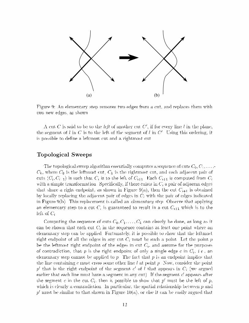
Figure �� An elementary step removes two edges from a cut� and replaces them withtwo new edges� as shown�

A cut C is said to be to the left of another cut C �� if for every line l in the plane�the segment of l in C is to the left of the segment of l in C �� Using this ordering� itis possible to de�ne a leftmost cut and a rightmost cut�

Topological Sweeps

The topological sweep algorithm essentially computes a sequence of cuts C�� C�� � � � ��Ck� where C� is the leftmost cut� Ck is the rightmost cut� and each adjacent pair ofcuts �Ci� Ci�� is such that Ci is to the left of Ci��� Each Ci�� is computed from Ci

with a simple transformation� Speci�cally� if there exists in Ci a pair of adjacent edgesthat share a right endpoint� as shown in Figure ��a� then the cut Ci�� is obtainedby locally replacing the adjacent pair of edges in Ci with the pair of edges indicatedin Figure ��b� This replacement is called an elementary step� Observe that applyingan elementary step to a cut Ci is guaranteed to result in a cut Ci�� which is to theleft of Ci�

Computing the sequence of cuts C�� C�� � � � � Ck can clearly be done� as long as itcan be shown that each cut Ci in the sequence contains at least one point where anelementary step can be applied� Fortunately� it is possible to show that the leftmostright endpoint of all the edges in any cut Ci must be such a point� Let the point pbe the leftmost right endpoint of the edges in cut Ci� and assume for the purposesof contradiction� that p is the right endpoint of only a single edge c in Ci� i�e�� anelementary step cannot be applied to p� The fact that p is an endpoint implies thatthe line containing c must cross some other line l at point p� Now� consider the pointp� that is the right endpoint of the segment c� of l that appears in Ci �we arguedearlier that each line must have a segment in any cut� If the segment c� appears afterthe segment c in the cut Ci� then it possible to show that p� must be the left of p�which is clearly a contradiction� In particular� the spatial relationship between p andp� must be similar to that shown in Figure ���a� or else it can be easily argued that

��

p

p'

p'

p

(a) (b)

Figure ���

the �above� ordering contains a cycle� which previously was shown to be impossible�Similarly� if the segment c� appears before the segment c in the cut Ci� then the spatialrelationship between p and p� must be similar to that shown in Figure ���b� and onceagain� the contradictory conclusion that p� is to the left of p can be drawn� Thus�since c� must either appear before or after c in Ci� p must be right endpoint of twosegments in Ci� and consequently is a point where an elementary step can be applied�The preceding argument is not valid for the rightmost cut of the arrangement� butthis is of no consequence� since the rightmost cut is always the last in the sequenceC�� C�� � � � � Ck�

Since it is always possible to �nd a pair of edges that share a right endpoint� andgiven the fact that each line in the plane must have exactly one segment in eachcut� it becomes apparent that each cut essentially speci�es a permutation of the linesin the plane �the leftmost cut corresponds to the permutation that lists all lines ininverse�slope order� while each elementary step corresponds to a transposition of twoadjacent lines in a particular permutation� In the algorithm using the �vertical� sweepline� the order of the transpositions was determined by the x�coordinate orderingof all the intersections of the n lines� By switching to a topological sweep line� itbecomes possible to perform the transposition on any suitable pair of edges� whilestill obtaining the desired arrangement� By eliminating the need to compute the x�coordinate ordering� it is possible to reduce the amount of time needed to computethe arrangement�

Horizon Trees

At this point� the overall structure of the topological sweep algorithm is easily stated�The algorithm begins with the leftmost cut� and maintains a �bag� of points thatelementary steps can be applied to� The algorithm then proceeds to pull a point

��

from the bag� perform an elementary step� check for new points that belong in thebag� and add any new points that are discovered� What remains to be described�are methods for generating the leftmost cut� and �nding new points that belong inthe bag� Observe� that the need to identify new points for the bag is particularlytroublesome� since a naive search would result in a �elementary step� that took O�ntime to perform� and an algorithms that was O�n� overall� Fortunately� both thesetasks can be performed using a complementary pair of data structures� the upper andlower horizon trees� By making use of horizon trees� the amortized time required foreach elementary step is constant�

The upper �lower� horizon tree of a cut c�� c�� � � � � cn�� is constructed by extendingthe edges in the cut to the right� and �killing� edges as they intersect� In particular�whenever two extended edges intersect� the edge of lower �higher slope no longercontinues to be extended� while edge of higher �lower slope continues on to the right�Formally� if the edges c�� c�� � � � � cn�� are part of the lines l�� l�� � � � � ln��� then a pointp on line li is part of the upper horizon tree� if

� p is above all lines lj� where j � i� and

� p is below all lines lk� where k � i and lk is of greater slope than li�

Similarly� a point p on line li is part of the lower horizon tree� if

� p is below all lines lj� where j � i� and

� p is above all lines lk� where k � i and lk is of lesser slope than li�

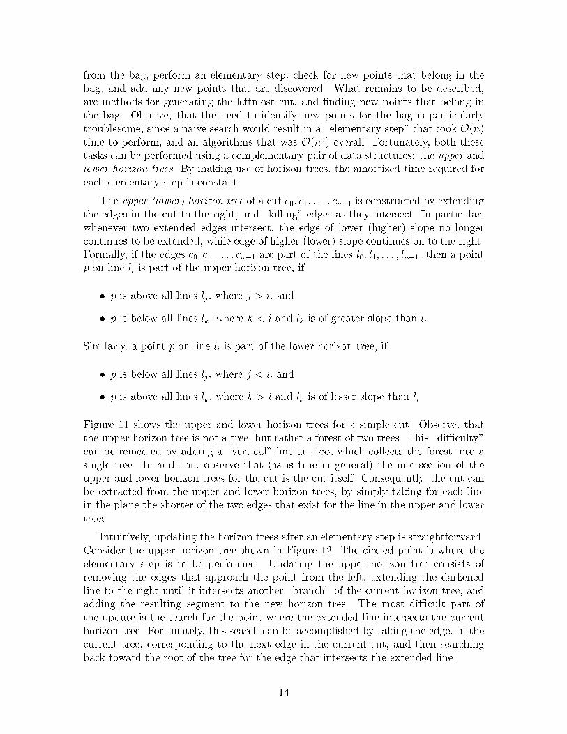
Figure �� shows the upper and lower horizon trees for a simple cut� Observe� thatthe upper horizon tree is not a tree� but rather a forest of two trees� This �di�culty�can be remedied by adding a �vertical� line at ��� which collects the forest into asingle tree� In addition� observe that �as is true in general the intersection of theupper and lower horizon trees for the cut is the cut itself� Consequently� the cut canbe extracted from the upper and lower horizon trees� by simply taking for each linein the plane the shorter of the two edges that exist for the line in the upper and lowertrees�

Intuitively� updating the horizon trees after an elementary step is straightforward�Consider the upper horizon tree shown in Figure ��� The circled point is where theelementary step is to be performed� Updating the upper horizon tree consists ofremoving the edges that approach the point from the left� extending the darkenedline to the right until it intersects another �branch� of the current horizon tree� andadding the resulting segment to the new horizon tree� The most di�cult part ofthe update is the search for the point where the extended line intersects the currenthorizon tree� Fortunately� this search can be accomplished by taking the edge� in thecurrent tree� corresponding to the next edge in the current cut� and then searchingback toward the root of the tree for the edge that intersects the extended line�

��

c0

c2

c1

c3

c4

c0

c2

c1

c3

c4

Upper Horizon Tree

Lower Horizon Tree

Figure ��� Upper and lower horizon trees for the indicated topological line�

Computing the upper horizon tree for the leftmost cut is accomplished in a similarfashion� Simply presort the lines in reverse slope order� and incrementally constructthe initial horizon tree by �inserting� the lines� in sorted order� with the updateroutine just described� Since newly inserted lines act as �shields� which prevent someparts of the tree from ever being examined during subsequent insertions� the totaltime to construct the initial upper horizon tree is O�n overall� The construction ofthe initial lower horizon tree is similar�

��

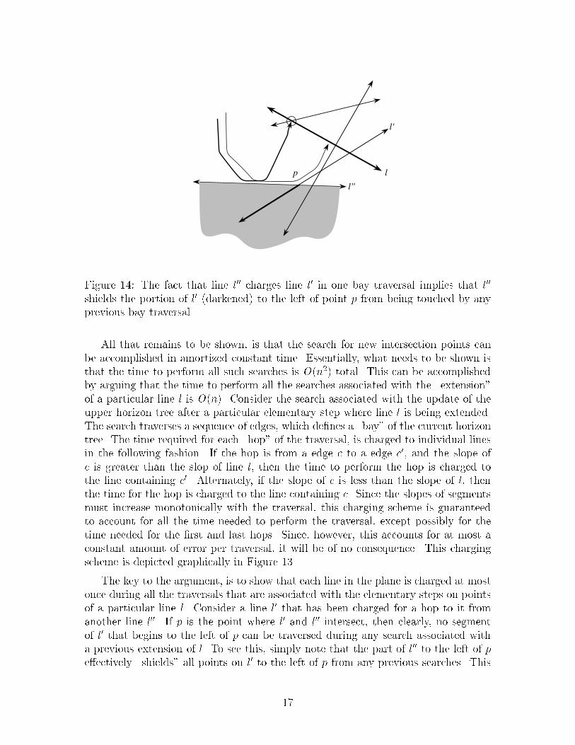
Figure ��� The basic update procedure for the upper horizon tree� Performing andelementary step on the circled point requires extending the darkened line� and search�ing along the �bay� to �nd where the extended line intersects the current tree� The�nal upper horizon tree is shown to the right�

Figure ��� Basic charging scheme for bay traversals� The circled point indicatesthe site of the elementary step being performed� while the broken line indicates theparallel support line that separates the bay into edges whose slopes are greater!lessthan the slope of the line being extended�

��

l

l'

l''

p

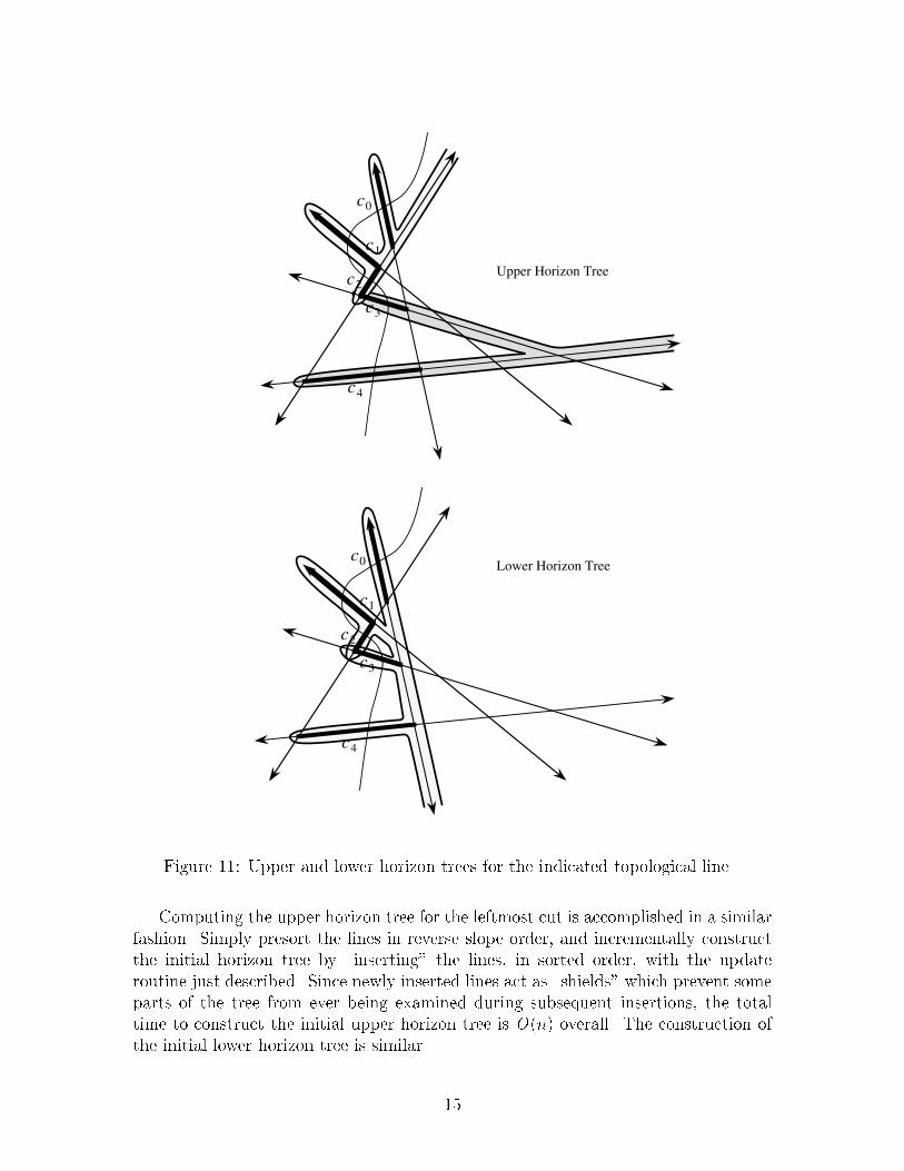
Figure ��� The fact that line l�� charges line l� in one bay traversal implies that l��

shields the portion of l� �darkened to the left of point p from being touched by anyprevious bay traversal�

All that remains to be shown� is that the search for new intersection points canbe accomplished in amortized constant time� Essentially� what needs to be shown isthat the time to perform all such searches is O�n� total� This can be accomplishedby arguing that the time to perform all the searches associated with the �extension�of a particular line l is O�n� Consider the search associated with the update of theupper horizon tree after a particular elementary step where line l is being extended�The search traverses a sequence of edges� which de�nes a �bay� of the current horizontree� The time required for each �hop� of the traversal� is charged to individual linesin the following fashion� If the hop is from a edge c to a edge c�� and the slope ofc is greater than the slop of line l� then the time to perform the hop is charged tothe line containing c�� Alternately� if the slope of c is less than the slope of l� thenthe time for the hop is charged to the line containing c� Since the slopes of segmentsmust increase monotonically with the traversal� this charging scheme is guaranteedto account for all the time needed to perform the traversal� except possibly for thetime needed for the �rst and last hops� Since� however� this accounts for at most aconstant amount of error per traversal� it will be of no consequence� This chargingscheme is depicted graphically in Figure ���

The key to the argument� is to show that each line in the plane is charged at mostonce during all the traversals that are associated with the elementary steps on pointsof a particular line l� Consider a line l� that has been charged for a hop to it fromanother line l��� If p is the point where l� and l�� intersect� then clearly� no segmentof l� that begins to the left of p can be traversed during any search associated witha previous extension of l� To see this� simply note that the part of l�� to the left of pe�ectively �shields� all points on l� to the left of p from any previous searches� This

�

l

l'

l'''pl''

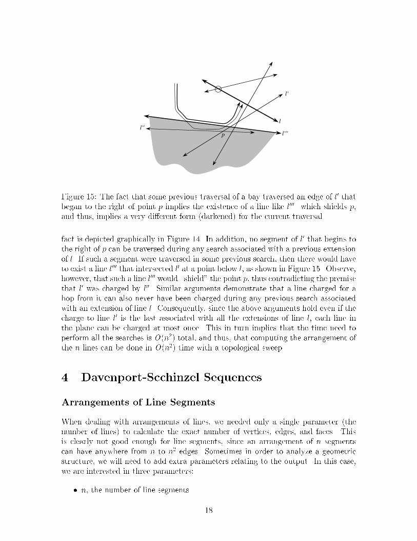
Figure ��� The fact that some previous traversal of a bay traversed an edge of l� thatbegan to the right of point p implies the existence of a line like l���� which shields p�and thus� implies a very di�erent form �darkened for the current traversal�

fact is depicted graphically in Figure ��� In addition� no segment of l� that begins tothe right of p can be traversed during any search associated with a previous extensionof l� If such a segment were traversed in some previous search� then there would haveto exist a line l��� that intersected l� at a point below l� as shown in Figure ��� Observe�however� that such a line l��� would �shield� the point p� thus contradicting the premisethat l� was charged by l��� Similar arguments demonstrate that a line charged for ahop from it can also never have been charged during any previous search associatedwith an extension of line l� Consequently� since the above arguments hold even if thecharge to line l� is the last associated with all the extensions of line l� each line inthe plane can be charged at most once� This in turn implies that the time need toperform all the searches is O�n� total� and thus� that computing the arrangement ofthe n lines can be done in O�n� time with a topological sweep�

� Davenport�Scchinzel Sequences

Arrangements of Line Segments

When dealing with arrangements of lines� we needed only a single parameter �thenumber of lines to calculate the exact number of vertices� edges� and faces� Thisis clearly not good enough for line segments� since an arrangement of n segmentscan have anywhere from n to n� edges� Sometimes in order to analyze a geometricstructure� we will need to add extra parameters relating to the output� In this case�we are interested in three parameters�

� n� the number of line segments

��

Figure ��� An arrangement with n � �� k � �� c � ��

� k� the number of intersections between segments� where � � k ��n�

�� c� the number of connected components in the arrangement

Using these parameters� we can determine the exact number of vertices� edges�and faces in the arrangement� As before� we will assume that there are no degen�eracies �i�e� no three segments ever coincide� and segments do not intersect at theirendpoints� Under these conditions there is one vertex for each endpoint� plus onefor each intersection� For edges there are n initially� and each intersection adds twomore �one for each of the segments that it splits� Hence we have

v � �n � k

e � n � �k�

To count faces we make use of Euler s Theorem �one of many which says thatv � f � e � c � � for any planar graph� �The constant at the end depends on thetopological properties of the space the graph is embedded into� Applying this toarrangements of line segments� we get

f � k � n � c � ��

The arrangement of �gure �� has �� vertices� �� edges� and � faces �one of which isthe outer face�

Lower Envelopes

We are interested in calculating upper bounds on the complexity of single faces andzones� just as we did for arrangements of lines� A useful concept in calculating thesebounds is the lower envelope of an arrangement� which can be de�ned as the portionof the arrangement visible from z � �� �see �gure �� The complexity of the lowerenvelope is simply the number of segment portions which are visible�

��

a

b

c

a b a c a c

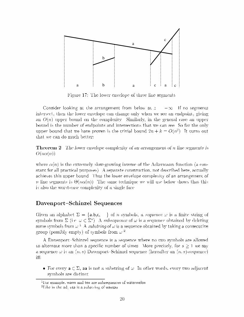
Figure �� The lower envelope of three line segments�

Consider looking at the arrangement from below at z � ��� If no segmentsintersect� then the lower envelope can change only when we see an endpoint� givingan O�n upper bound on the complexity� Similarly� in the general case an upperbound is the number of endpoints and intersections that we can see� So far the onlyupper bound that we have proven is the trivial bound �n � k � O�n�� It turns outthat we can do much better�

Theorem �� The lower envelope complexity of an arrangement of n line segments isO�n��n�

where ��n is the extremely slow�growing inverse of the Ackermann function �a con�stant for all practical purposes� A separate construction� not described here� actuallyachieves this upper bound� Thus the lower envelope complexity of an arrangement ofn line segments is ��n��n� The same technique we will use below shows that thisis also the worst�case complexity of a single face�

Davenport�Schinzel Sequences

Given an alphabet " � fa�b�c�� � � g of n symbols� a sequence � is a �nite string ofsymbols from " �i�e� � � "�� A subsequence of � is a sequence obtained by deletingsome symbols from ��� A substring of � is a sequence obtained by taking a consecutivegroup �possibly empty of symbols from ���

A Davenport#Schinzel sequence is a sequence where no two symbols are allowedto alternate more than a speci�c number of times� More precisely� for s � � we saya sequence � is an �n� s Davenport#Schinzel sequence �hereafter an �n� s�sequencei��

� For every a � "� aa is not a substring of �� In other words� every two adjacentsymbols are distinct�

�For example� warm and ten are subsequences of watermelon��Like in the ad� usa is a substring of wausau�

��

� For every pair of distinct symbols a� b � "� the sequence of s � � alternatinga s and b s is not a subsequence of �� Thus aba is forbidden if s � �� abab isforbidden if s � �� ababa is forbidden if s � �� and so on�

We are interested in estimating �s�n� the maximum length of any �n� s�sequence�As an initial exercise� it is easy to check that this function is bounded� i�e� �s�n ��for all s and n�

When s � � no symbol may appear twice� thus ���n � n� A slightly trickierargument shows that ���n � �n� �� achieved by � � ab� � �yzy� � �ba or abacad� � �aza�The �rst di�cult case is s � �� where ���n � O�n��n� We present below a �simple�proof of this result due to Peter Shor�

How does this relate to lower envelopes� Two line segments can intersect in atmost one place� It is easy to check that while the subsequence abab can occur in thelower envelope� the subsequence ababa cannot �it requires two intersections� Thusthe sequence of segments in the lower envelope is an �n� ��sequence �recall �gure ��The proof of Theorem � reduces to proving the bound on ���n mentioned above�

Lower envelopes and Davenport#Schinzel sequences arise naturally in many geo�metric problems� Often we will be dealing with geometric primitives where there issome small constant bound on the number of intersections between any pair �eg� linesegments� circles� polynomials� The lower envelope of a collection of such primitiveswill be a Davenport#Schinzel sequence of some small order� Fortunately� �s�n is�almost� linear for every s� ie� it is the product of n and some very slow�growingfunction� For example� ���n � ��n���n��

The Ackermann Function

Here we review the Ackermann function �which grows faster than any primitive re�cursive function� For each k � �� we de�ne a function Ak on the positive integers�

A��n � �n ��

Ak���n � A�n�k �� ��

where f �n� denotes the function f iterated n times� For example

A��n � �n�

A��n � �� ��� ���� a tower

of n � s�

A��n � �� ��� ���� � � �

���o

� g� �z �n towers

��

and so on �becoming increasingly di�cult to typeset� De�ne the Ackermann functionby diagonalization�

A�n � An�n� ��

��

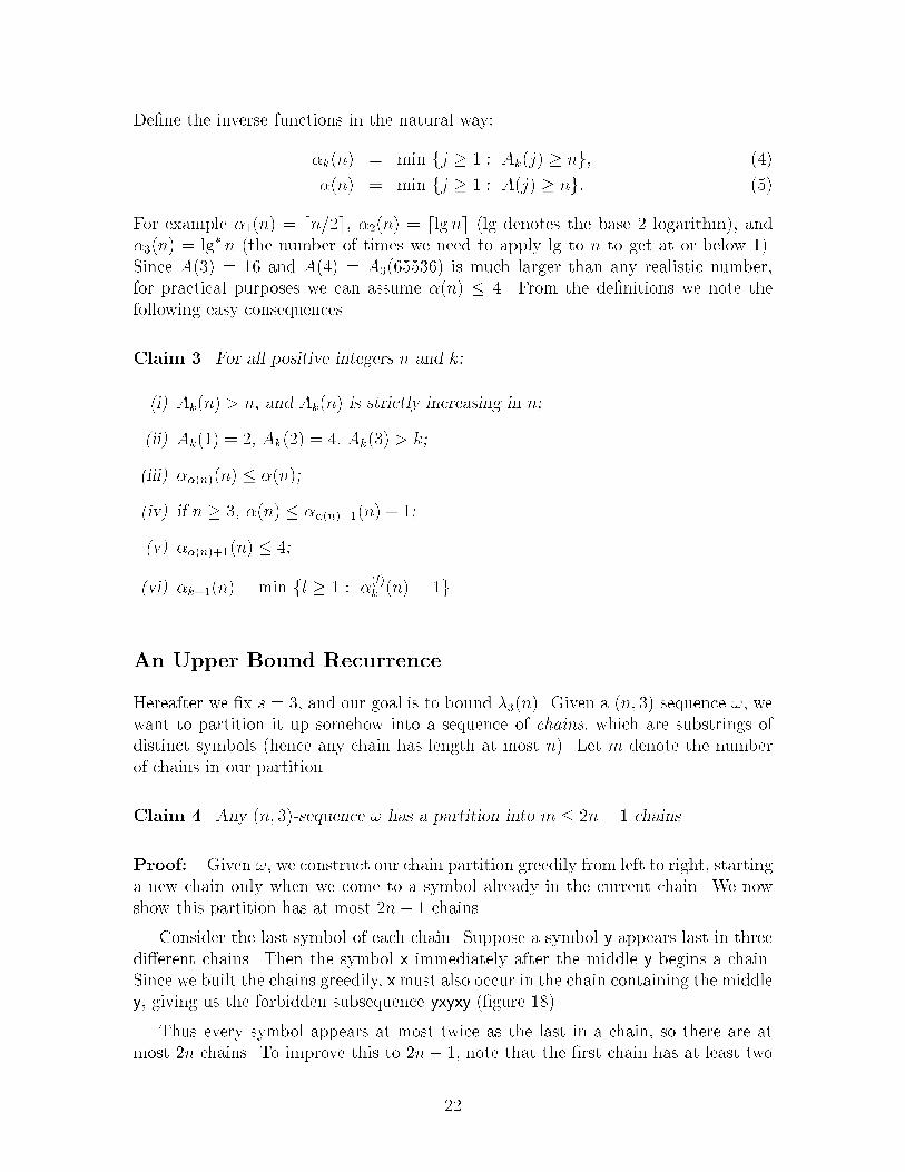
De�ne the inverse functions in the natural way�

�k�n � min fj � � � Ak�j � ng� ��

��n � min fj � � � A�j � ng� ��

For example ���n � dn��e� ���n � dlg ne �lg denotes the base � logarithm� and���n � lg� n �the number of times we need to apply lg to n to get at or below ��Since A�� � �� and A�� � A������� is much larger than any realistic number�for practical purposes we can assume ��n � �� From the de�nitions we note thefollowing easy consequences�

Claim �� For all positive integers n and k�

�i� Ak�n � n� and Ak�n is strictly increasing in n�

�ii� Ak�� � �� Ak�� � �� Ak�� � k�

�iii� ���n��n � ��n�

�iv� if n � �� ��n � ���n����n � ��

�v� ���n����n � ��

�vi� �k���n � min fl � � � ��l�k �n � �g�

An Upper Bound Recurrence

Hereafter we �x s � �� and our goal is to bound ���n� Given a �n� ��sequence �� wewant to partition it up somehow into a sequence of chains� which are substrings ofdistinct symbols �hence any chain has length at most n� Let m denote the numberof chains in our partition�

Claim �� Any �n� ��sequence � has a partition into m � �n� � chains�

Proof� Given �� we construct our chain partition greedily from left to right� startinga new chain only when we come to a symbol already in the current chain� We nowshow this partition has at most �n� � chains�

Consider the last symbol of each chain� Suppose a symbol y appears last in threedi�erent chains� Then the symbol x immediately after the middle y begins a chain�Since we built the chains greedily� x must also occur in the chain containing the middley� giving us the forbidden subsequence yxyxy ��gure ���

Thus every symbol appears at most twice as the last in a chain� so there are atmost �n chains� To improve this to �n� �� note that the �rst chain has at least two

��

x y xy y

Figure ��� A symbol appearing last in three di�erent chains�

symbols� Consider the second�last symbol of the �rst chain� and the same argumentshows that it cannot occur last in two other chains� �

We have already shown ���n � �n�� Our re�ned analysis of ���n will recursivelyneed to keep track of m� so we de�ne �m�n to be the maximum length of a �n� ��sequence with a partition into at most m chains� Thus ���n � ��n � �� n� Wenote the trivial bound �m�n � mn� which we will use as a base case when m � ��

Theorem �� Given n�m� and � � b � m� there exists a partition n � n��� � ��nb�n�such that

�m�n � �b� �� n� �bX

i�

�dm�be� ni � �m � �n��

Proof� Let � be a maximum length m�chain �n� ��sequence� We begin by cutting� into b blocks� each consisting of c � dm�be consecutive chains each �the last blockmay have less than c chains� We call a symbol internal if it appears in only oneblock� otherwise we call it external� Let ni denote the number of internal symbols inthe i�th block� and let n� denote the number of external symbols� this gives us ourpartition of n�

Consider the subsequence of internal symbols in the i�th block� This subsequencewould be an �ni� ��sequence except that it may have repetitions� Since repetitionsmay only occur at chain boundaries� we may delete at most one symbol at each bound�ary within the block to remove all repetitions� After these deletions� the remainingsymbols are an �ni� ��sequence� and hence there are at most �c� ni internal symbolsleft in the block� Summing over all blocks� at most m internal symbols are deleted�and at most

Pbi� �c� ni internal symbols remain in the �ni� ��subsequences�

Now we need to count the external symbols� We divide the appearances of theexternal symbols into three kinds� middle� �rst� and last appearances� An occurrenceof x is a middle appearance if x occurs in both an earlier and a later block� Anoccurrence of x is a �rst appearance if x does not appear in any earlier block� since x

is external� x must appear in a later block� Last appearances are de�ned symmetrically��gure ���

Consider the subsequence of middle appearances of external symbols� First weneed to �x any repetitions� as before� we need delete at most one symbol per chainboundary� for at most m deletions� Call the resulting sequence ���

Claim �� No symbol of �� appears twice in the same block�

��

x xx x x

first middle last

block block block

Figure ��� First� middle� and last appearances of x�

x

block block block

xyy y

first last

Figure ��� A symbol of �� appearing twice in the same block�

Proof� If x appeared twice in the same block of ��� then some other externalsymbol y must appear between these two occurences in ��� Since this y is a middleappearance in �� y also appears in earlier and later blocks of �� giving us the forbiddensubsequence yxyxy in � ��gure ��� �

Thus the b blocks of � have become chains for ��� Since no symbol of �� appearsin the �rst or last block� �� has a decomposition into at most b� � chains� Hence ��

has length at most �b� �� n��

Now all we have left to count are the �rst and last appearances of external symbols�We argue a bound on �rst appearances� last appearances are handled symmetrically�Consider the subsequence of all �rst appearances of external symbols� As before�eliminate all repetitions using at most m deletions� let �FIRST be the resulting sequence�

Claim �� The sequence �FIRST is an �n�� ��sequence�

Proof� Suppose xyxy appears as a subsequence of �FIRST for some distinct externalsymbols x and y� Then these four appearances must all occur in the same block of� �since all �rst appearances of a symbol occur in the same block� Since the x s are�rst appearances� there must be another appearance of x in a later block� giving usthe forbidden subsequence xyxyx in �� �

Thus �FIRST has length at most ���n� � �n�� so there are at most �n� � m �rst

appearances of external symbols altogether� Likewise for last appearances� We haveaccounted for all the symbols of �� so adding all the terms proves the recurrence� �

��

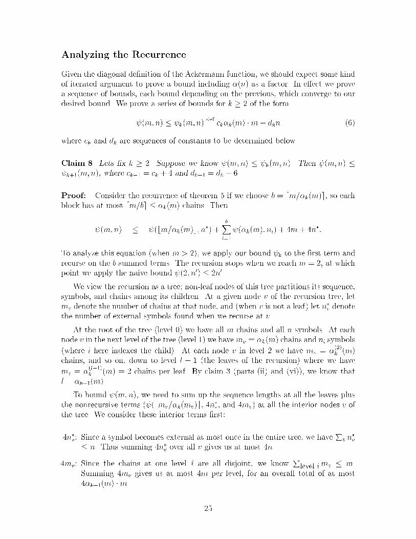
Analyzing the Recurrence

Given the diagonal de�nition of the Ackermann function� we should expect some kindof iterated argument to prove a bound including ��n as a factor� In e�ect we provea sequence of bounds� each bound depending on the previous� which converge to ourdesired bound� We prove a series of bounds for k � � of the form

�m�n � k�m�ndef� ck�k�m �m � dkn ��

where ck and dk are sequences of constants to be determined below�

Claim � Lets �x k � �� Suppose we know �m�n � k�m�n� Then �m�n �k���m�n� where ck�� � ck � � and dk�� � dk � ��

Proof� Consider the recurrence of theorem � if we choose b � dm��k�me� so eachblock has at most dm�be � �k�m chains� Then

�m�n � �bm��k�mc� n� �bX

i�

��k�m� ni � �m � �n��

To analyze this equation �when m � �� we apply our bound k to the �rst term andrecurse on the b summed terms� The recursion stops when we reach m � �� at whichpoint we apply the naive bound ��� n� � �n��

We view the recursion as a tree� non�leaf nodes of this tree partitions its sequence�symbols� and chains among its children� At a given node v of the recursion tree� letmv denote the number of chains at that node� and �when v is not a leaf let n�v denotethe number of external symbols found when we recurse at v�

At the root of the tree �level � we have all m chains and all n symbols� At eachnode v in the next level of the tree �level � we have mv � �k�m chains and ni symbols

�where i here indexes the child� At each node v in level � we have mv � ����k �m

chains� and so on� down to level l � � �the leaves of the recursion where we have

mv � ��l���k �m � � chains per leaf� By claim � �parts �ii and �vi� we know that

l � �k���m�

To bound �m�n� we need to sum up the sequence lengths at all the leaves plusthe nonrecursive terms ��bmv��k�mvc� �n�v� and �mv at all the interior nodes v ofthe tree� We consider these interior terms �rst�

�n�v� Since a symbol becomes external at most once in the entire tree� we haveP

v n�v

� n� Thus summing �n�v over all v gives us at most �n�

�mv� Since the chains at one level i are all disjoint� we knowP

level imv � m�Summing �mv gives us at most �m per level� for an overall total of at most��k���m �m�

��

�bmv��k�mvc� n�v�This is where we apply our given k bound� We estimate

�bmv��k�mvc� n�v � k�bmv��k�mvc� n�v� ck �k�bmv��k�mvc � bmv��k�mvc� dkn

�v

� ck �k�mv � bmv��k�mvc� dkn�v

� ckmv � dkn�v�

To sum this over all interior nodes v� we reapply the estimates of the last twocases� getting the bound ck�k���m �m � dkn�

Now the leaf terms are easy to count up� since di�erent leaves count disjoint setsof symbols and have at most mv � � chains each� the leaf terms altogether contributeat most �n at the bottom of the unfolded recurrence�

Adding everything up gives �m�n � �n � ��k���m �m � ck�k���m �m � dkn� �n � ck���k���m �m � dk��n � k���m�n� �

We are almost done� we just need to show how to get started with values for c�and d�� and also how to choose a good value for k to balance n�

Claim � �m�n � ��m�n � c�mdlgme � d�n� where c� � � and d� � ��

Proof� We follow a simpli�ed version of the previous argument� We take b � � oneach step� Since we divide the sequence into only two blocks� there are no middleappearances of external symbols �i�e� �� is empty� so we have the simpler recurrence

�m�n ��X

i�

�dm��e� ni � �m � �n��

where the �m in the general theorem may be reduced to �m in this special case� Ourrecurrence tree has leaves at level l � � where l � ���m � dlgme� Now summingterms as before �again getting �n from the leaves� we get the claimed bound� �

Corollary ��� For every k � �� �m�n � ��k � ��k�m �m � ��k � �n�

Theorem ��� ���n � O�n � ��n�

Proof� Setting m � �n� we have ���n � �m�n � O�k��k�m � m � n �O�k �k�n � n for all k � �� It now su�ces to take k just large enough so that�k�n � O��� By part �v of claim �� it su�ces to take k � ��n � �� �

��

� Arrangements in Higher Dimensions

Overview

Until now� we have looked at arrangements of lines in the plane� We shall now take ashort digression and consider higher dimensional versions of the problem� After somede�nitions� this lecture will be dedicated to generalizing the zone theorem to higherdimensions�

De�nitions

De�nition ��� Ed is the d�dimensional Euclidean space�

De�nition ��� A hyperplane in Ed is a d� � dimensional linear subspace�

De�nition ��� A k��at is a k�dimensional linear subspace� An intersection of d� khyperplanes forms a k��at�

De�nition ��� The codimension of a k�dimensional subspace of Ed is d� k�

Counting Objects in the Arrangement

Recall that an arrangement of lines in the plane creates the following structures�objects of dimension � �vertices� of dimension � �edges� and of dimension � �faces�A similar phenomenon takes place in an arrangement of n hyperplanes in Ed� onlynow structures of all dimensions between � and d� collectively called faces� are created�We will carry over a lot of the terminology from � dimensions� ��dimensional objects�points will be called vertices� ��dimensional objects are edges� �d � ��dimensionalobjects are called facets� d dimensional objects are called cells� The terms facet andcell make a great deal of sense if we consider the case d � �� i�e� the arrangementis a collections of planes in ��dimensional space� As in the ��dimensional case� eachfacet is part of the boundary of a cell� and in general each face of dimension i is aboundary of a face of dimension i � ��

We begin as we did in the ��dimensional case� by studying the number of verticesformed� Assuming no degeneracies� each group of d hyperplanes intersects to de�nea single vertex� Thus the number of vertices is just the number of ways to choosed hyperplanes from the arrangement� i�e�

�nd

�� Counting higher dimensional faces

requires more work�

Lemma ��� The number of cells in an arrangement of n hyperplanes in Ed isn

d

�

n

d� �

� � � ��

n

�

�

n

�

�

Proof� Recall the ��dimensional proof� We let each vertex correspond to the faceof which it was the bottom vertex� which gave

�n�

�faces� and we then had to count

the faces with no bottom vertex� namely those which were unbounded below� To dothis� we drew a horizontal line below all the vertices� It clearly passed through n� �faces� since it intersected each line in the arrangement exactly once� and entered anew face at each intersection� This gave the result we needed� To generalize to the ddimensional case� do the same thing� Each cell bounded from below corresponds to avertex� namely the lowest vertex in that cell �where �lowest� is measured according tothe last dimension� It remains to count the unbounded cells� If we draw a hyperplaneH perpendicular to the last dimension and below all the vertices� our n hyperplanesin Ed each intersect H in a �d � ��dimensional space� Thus these n hyperplanesimpose an arrangement of n �d� ��dimensional hyperplanes in H� Each cell in thisarrangement corresponds to one of the unbounded cells in the original arrangement�The result then follows by induction� �

Lemma ��� The number of faces of codimension k in an arrangement of hyperplanesin Ed is�

n

k

X��j�d�k

n� k

j

�

Proof� Each such face �lives in� some �d�k��at� The total number of such faces

is thus equal to the total number of �d�k��ats� namely�nk

�� times the number of faces

living in a single �at� This can be determined using the previous theorem� becausefor each such �d � k��at� which is an intersection of k hyperplanes� the remainingn � k hyperplanes impose an arrangement in that �at� namely an arrangement ofn � k hyperplanes in d � k dimensions� Each cell �from the perspective of this newarrangement is a �d� k dimensional face of the original arrangement� �

This number of faces can be written more cleanly as

dXjk

n

j

j

k

�

The Zone Theorem in Higher Dimensions

We now come to the main topic of this lecture� namely the zone theorem in higherdimensions�

Theorem � The Zone Theorem�� The zone of a hyperplane in an arrangementof n hyperplanes in Ed has complexity ��nd��� counting all faces of all dimensions�

Proof� Let H be the original set of n hyperplanes� and A�H the arrangementde�ned by them� We consider some new hyperplane b and want to study the cells

��

which are in the zone of b in H� written zone�b�H� Let

zk�b�H �X

c�zone�b�H�

�the number of faces of codimension k in c

zk�n� d � maxb�H

zk�b�H�

Our goal is to show that zk�n� d � O�nd�� �showing the corresponding lower boundis left as an exercise� We will do this by �rst proving and then analyzing the followingrecursion� which we claim holds for every d � �� � � k � d� and n � k�

zk�n� d � n

n� k�zk�n� d� � � zk�n� �� d� �� �

A caveat� by counting over all cells individually� we are actually overcounting thezone complexity� since� e�g� a vertex appears in many cells� and so we count it manytimes� To identify each counting of a given face� de�ne a border of codimension kto be a pair �f� C where f is a k�codimensional face and C is a cell that has f asa boundary� Since we will count the total number of borders� our result is actuallystronger than just counting the total complexity� But the bound is shown to holdeven with this overcounting� This is fortunate� since often we need to overcount forapplications in precisely this way�

We will prove Equation by induction on the number of hyperplanes in thearrangement� Let H be some arrangement� and let b be the new hyperplane� Foreach hyperplane h � H� we will consider the e�ect of removing h� Let H�h denotethe arrangement induced by H in the hyperplane h� i�e� the �d � ��dimensionalarrangement of hyperplanes fj h j j � Hg� Consider the quantity

zk�b�H � fhg � zk�b h�H�h

We claim that this counts all the borders �f� C of codimension k in zone�b�H withf � h� To see this� consider what happens when we remove h from the arrangement�Since f is not in h� f remains part of the zone� although it may now merge with someother faces from which it was previously separated by h� Consider some cell C in b szone with h removed� If h does not cut C� then every border in C in the originalarrangement is counted by the �rst term in the above equation� The same holds trueif h does cut C� but only one of the two resulting cells is in the zone of b� This is truesince for any border which is cut by h� one of the two resulting borders is a borderfor the cell not in b s zone� The only case which can cause trouble is if both of thecells formed by h splitting C are in the zone of b� But for this to happen h must hitb within C� This being the case� the second term counts what happens� each bordersuch that both halves are seen by b forms �by intersection with h a k�codimensionalborder in the zone of b in the arrangement of H�h�

Now apply this argument to each of the n planes in h� Each time we remove ahyperplane� we count all the borders not in that hyperplane using the above equation�Thus each border is counted once each time we remove a hyperplane which does

��

not contain it� Since the border is in a �d � k��at� which is an intersection of khyperplanes� this happens n� k times� Thus

�n� kzk�b�H �Xh�H

�zk�b�H � fhg � zk�b h�H�h

� Xh�H

�zk�n� �� d � zk�n� �� d� �

� n�zk�n� �� d � zk�n� �� d� ��

Since the proof holds for any choice of arrangement� it must hold for the arrange�ment which gives the maximum count� Equation then follows�

It remains to analyze the inequality in Equation � This is straightforward� If welet

wk�n� d ��n� k

n zk�n� d � O�

zk�n� d

nk

Then our recurrence becomes

wk�n� d � wk�n� �� d � wk�n� �� d� �� ��

We will now prove the result by induction on n and d� We have already proved thetwo dimensional zone theorem� which tells us that for d � �� zk�n� � � O�n� Thisgives the base case for the induction� Now assume we have proved the result for d���and prove it for d� Assume �rst that k � d� �� Unwinding the recurrence gives

wk�n� d �nX

j�

wk�j� d� � � wk�d� d�

Note that wk�d� d is just a constant �though it depends on d� By our inductionhypothesis� wk�n� d � O�nd���k� We can thus rewrite the equation as

wk�n� d �nX

j�

O�jd���k � O��

� O�nd���k�

and the result for zk follows� What remains are the cases k � d or k � d � ��Unfortunately� the above recurrence isn t powerful enough�solving it for these valuesof k overestimates the result by a factor of log n� We thus turn to a di�erent tool�Euler s Theorem�

De�nition �� For a cell c� let gk�c be the number of facets of codimension kbounding c�

Theorem �� Euler�s Theorem��

dXi�

���d�kgk�c �

�� if c is unbounded� otherwise�

��

If we apply this theorem to our arrangement� and sum over all cells in the zone� weget

dXk�

���d�kzk�b�H � ��

If we now move all the zk whose values we have already bounded to the right side ofthe equation� we get

zd���b�H� zd�b�H �d��Xk�

���d�kzk�b�H

� O�nd���

Note that zd�� is the number of edges and zd the number of vertices of the ar�rangement� We therefore claim that

dzd�b�H � �zd���b�H

To see this� observe that a given vertex is at the end of at least d edges� since a vertexis the intersection of d hyperplanes� the intersection of any d� � of these hyperplanesforms an edge with the vertex as an endpoint� On the other hand� every edge canhave at most two vertices as endpoints� Thus the left hand side is an undercount ofthe number of edge�endpoint pairs� since each vertex is in at least d such pairs� Onthe other hand� the right hand side is an overcount of the number of such pairs� sinceeach edge is in at most two of them�

Combining these two equations gives

��� ��dzd���b�H � zd���b�H� zd�b�H

� O�nd���

Therefore zd���b�H � O�nd��� and similarly zd�

�

� Voronoi Diagrams and Delaunay Triangulations

This section deals with two methods of solving proximity problems� Voronoi diagramsand Delaunay Triangulation� These fundamental diagrams are duals of one another�We will begin by presenting some preliminary facts about these diagrams�

Voronoi Diagrams

We are given n sites �points in the plane� for any given point� we wish to knowwhich site �or sites is closest� This problem has been referred to as the �post�o�ce

��

4 sites4 sites3 sites2 sites1 site

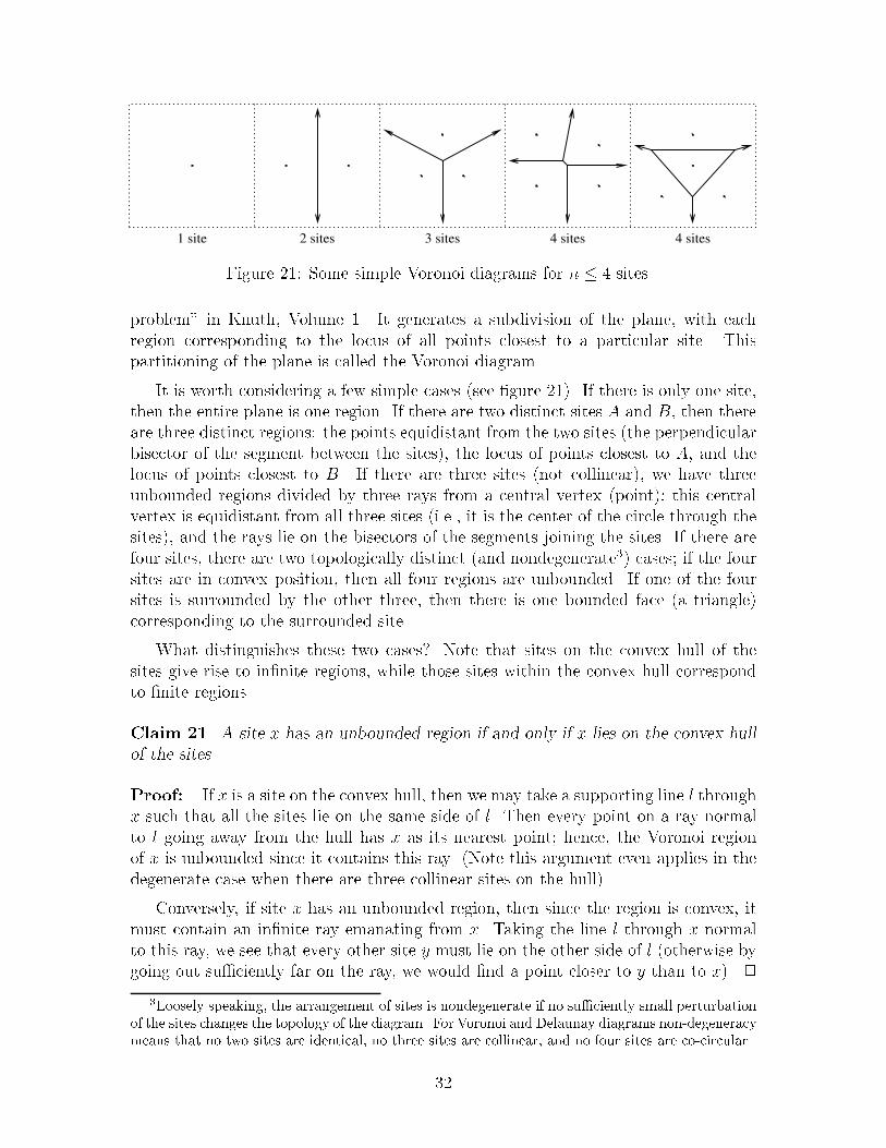
Figure ��� Some simple Voronoi diagrams for n � � sites�

problem� in Knuth� Volume �� It generates a subdivision of the plane� with eachregion corresponding to the locus of all points closest to a particular site� Thispartitioning of the plane is called the Voronoi diagram�

It is worth considering a few simple cases �see �gure ��� If there is only one site�then the entire plane is one region� If there are two distinct sites A and B� then thereare three distinct regions� the points equidistant from the two sites �the perpendicularbisector of the segment between the sites� the locus of points closest to A� and thelocus of points closest to B� If there are three sites �not collinear� we have threeunbounded regions divided by three rays from a central vertex �point� this centralvertex is equidistant from all three sites �i�e�� it is the center of the circle through thesites� and the rays lie on the bisectors of the segments joining the sites� If there arefour sites� there are two topologically distinct �and nondegenerate� cases� if the foursites are in convex position� then all four regions are unbounded� If one of the foursites is surrounded by the other three� then there is one bounded face �a trianglecorresponding to the surrounded site�

What distinguishes these two cases� Note that sites on the convex hull of thesites give rise to in�nite regions� while those sites within the convex hull correspondto �nite regions�

Claim ��� A site x has an unbounded region if and only if x lies on the convex hullof the sites�

Proof� If x is a site on the convex hull� then we may take a supporting line l throughx such that all the sites lie on the same side of l� Then every point on a ray normalto l going away from the hull has x as its nearest point� hence� the Voronoi regionof x is unbounded since it contains this ray� �Note this argument even applies in thedegenerate case when there are three collinear sites on the hull�

Conversely� if site x has an unbounded region� then since the region is convex� itmust contain an in�nite ray emanating from x� Taking the line l through x normalto this ray� we see that every other site y must lie on the other side of l �otherwise bygoing out su�ciently far on the ray� we would �nd a point closer to y than to x� �

�Loosely speaking� the arrangement of sites is nondegenerate if no su�ciently small perturbationof the sites changes the topology of the diagram� For Voronoi and Delaunay diagrams non�degeneracymeans that no two sites are identical� no three sites are collinear� and no four sites are co�circular�

��

Figure ��� The Voronoi diagram �solid and the Delaunay diagram �dashed��

Claim ��� All the Voronoi regions are convex�

Proof� Fix a site x� For every other site y� the Voronoi region of x is containedin the half�plane of points that are at least as close to x as they are to y� Thus�the Voronoi region of x is exactly the intersection of all such half�planes for di�erentsites y� Since each half�plane is convex and the intersection of convex regions is alsoconvex� the Voronoi region of x is convex� Note this argument also shows that theboundary of the Voronoi region of x is polygonal �i�e�� it is bounded by line segmentsor rays� �

Note that each vertex or edge of the Voronoi diagram depends on only a boundednumber of the sites� a vertex is de�ned by its three nearest sites� and an edge isde�ned by four sites # the two sites on whose bisector it lies� and two other sitesdelimiting its extent� This ��nite dependency� property will arise in many othersettings in geometric algorithms� Thus� if we compute the coordinates of one of thevertices of the diagram� those coordinates are low degree rational functions in thecoordinates of the three sites that de�ne it� But still it would be useful to computea diagram with no �new� real numbers� and this motivates the Delaunay diagram�

Delaunay Triangulations

The Delaunay triangulation is the graph theoretic dual� topological dual� or the com�binatorial theoretic dual of the Voronoi diagram �see �gure ��� the vertices of theDelaunay triangulation are the sites �corresponding to the regions of the Voronoidiagram� and we connect two sites with an edge in the Delaunay triangulation i�their Voronoi regions share an edge �thus� the two diagrams have the same numberof edges� although the Delaunay triangulation has no unbounded edges� Thus� avertex in the Voronoi diagram corresponds to a Delaunay triangle� a Voronoi edgeto a Delaunay edge� and a Voronoi face to a Delaunay vertex �site� Note� however�that dual edges of the two graphs do not necessarily intersect� Furthermore� we may

�This �gure swiped from page ��� of �GS��

��

a

b

x

y

Figure ��� Two circles cannot cross at � points�

recover the Voronoi diagram by reversing the process� Note there are no $new realnumbers needed to describe the Delaunay triangulation�

We now prove various simple properties of the Delaunay triangulation� In par�ticular� we present the notion that site�free circles through two or three sites are�witnesses to Delaunay�hood� for edges or triangles� respectively�

Claim ��� For every edge ab in the Delaunay triangulation� there is a circle� calleda witness� through sites a and b that contains no other site� The converse is also true�

Proof� Since a and b are connected� their Voronoi regions must share an edge� Takea point p in the interior of this edge� then a and b are the same distance r from p�and all other sites are further away� Hence� the circle of radius r about p su�ces�

Conversely� the existence of a circle through a and b with all other sites strictlyoutside implies that the center of the circle is on a boundary edge between the Voronoiregions of a and b� �

Claim ��� The Delaunay triangulation is planar�

Proof� It su�ces to prove that no two edges may cross� Suppose edges ab and xyappear in the Delaunay triangulation� and these edges cross� Then there is a circlethrough a and b not containing x or y� and likewise there is a circle through x andy not containing a or b� But then these two distinct circles must intersect at fourpoints� which is impossible� See �gure ��� �

Various other properties may also be argued� If abc is a triangle in the Delaunaytriangulation� then no other site lies inside its circumcircle� and conversely�

We now turn to counting problems� We will assume non�degeneracy �i�e�� no fourpoints are co�circular� no three points are collinear� We will make precise claimsabout the number of edges and triangles in the triangulation�

Let n be the number of sites� t the number of triangles� and e the number of edges�From Euler s Theorem for connected planar graphs� we have

n� e � t � � � �

��

orn� e � t � �

where t�� is the number of faces �each triangle is a face and so is the single unboundedface� We need one more parameter to describe the arrangement� Since each edgebelongs to two faces� we have �t � k � �e� where k is the number of sites on theconvex hull� Solving� we have

e � ��n� �� k�

t � ��n� �� k�

By duality� the Voronoi diagram will have e edges �bounded or unbounded and t ver�tices� Hence� these graphs have only linear complexity in the size of the input� whichwill be very important to the computational complexity of various planar proximityproblems� For example� this linear complexity implies that the corresponding datastructures can be stored in O�n space and that the arrangement can be computed inO�n logn time� However� this only holds for two dimensions� For the d�dimensional

case� we have O�nb d��� c complexity�

The Delaunay triangulation is somewhat more intuitive than the Voronoi dia�grams� so we will tend to use the Delaunay triangulation in this write�up� Anothercomment� Since the triangulation starts with numerical data and ends up with com�binatorial output �e�g� a graph� complications may arise due to round�o� errors�etc�

Delaunay triangulations are used in many applications �e�g�� �nite element analy�sis� interpolation� This triangulation is especially useful because it is easy to computeand it provides a �nice� triangulation �i�e�� the smallest angle in the triangulation isthe largest possible�

Suppose we have n sites� and someone claims a given triangulation is a Delaunaytriangulation� How much work do we have to do to verify the claim� If for each siteand each triangle we verify that the site is not in the circumcircle of the triangle� thenthis is clearly su�cient� Unfortunately� this is an O�n� time algorithm�

Delaunay proved a remarkable theorem� that it su�ces to only check adjacenttriangles� so that the veri�cation may be performed in linear time�

Theorem ��� Given a triangulation of n sites such that for every pair of adjacenttriangles abc and bcd� a is not in the circumcircle of bcd� then that triangulation isthe Delaunay triangulation�

Proof� First� we de�ne the �power� of a point with respect to a circle� Given apoint x and a circle C� draw a line l through x that intersects C at two points a andb� Then the power of the point is xa �xb �here xa denotes the distance from x to a� Itturns out that this quantity is independent of the line chosen� Furthermore� given asuitable choice of signs for distances along the line� the sign of the power determines

��

l

b

ax

b

ax

Figure ��� The power of point x with respect to the circle is ax � bx� which is inde�pendent of the choice of line l�

k

l

m

n

xd

Figure ��� The power of x with respect to lmn is less than the power of x with respectto klm�

whether x is inside� outside� or on the circle �the usual convention makes the powerpositive i� x is outside the circle�

Take a triangle abc of the given triangulation and a site x that lies on the oppositeside of �say line bc� If the neighboring triangle to abc along bc is xbc� then we aredone by assumption�

Otherwise� consider the line connecting site x to a point d in the interior of triangleabc� As we move along xd from x to d� we pass through a sequence of triangles� startingwith a triangle having x as a vertex �call it vwx and ending with triangle abc�

Now consider the sequence of circumcircles of these triangles� We start with thecircumcircle of vwx where the power of x is � �since x is on the circle� We claimthat the power of x can only increase as we move to circumcircles of triangles furtheraway from x� This claim implies that the power of x with respect to the circumcircleof abc must be positive� so that x is not in the circumcircle of abc� which is what wewanted to prove�

We now argue our claim informally� Given adjacent triangles lmn and klm onthe line from x to d �see �gure ��� consider their circumcircles� These circumcirclesare both members of the family of circles through l and m� and we may continuously�push� the circumcircle of lmn away from site n until it reaches site k� During thispush operation� both intersection points of the circle with xd move further away fromx� hence the power of x increases� �

��

� Geometric Primitives and A Delaunay Triangu�

lation Algorithm

In the �rst part of this lecture� we are going to introduce two geometric primitiveswhich enable us to extract some fundamental combinatorial properties of points� Inthe second part� we will introduce an algorithm based on the divide and conquer ideafor the Delaunay triangulation�

Geometric Primitives

Computational geometry problems are characterized by relations among geometricentities �vertices� edges� ��� and many of these relations can be described quantita�tively by real numbers� But many geometric algorithms are combinatorial by nature�So we need to have a conversion scheme� Geometric primitives are used to extractcombinatorial information from the input real numbers� the geometric primitives willmap the real numbers to bits �hence these primitives may also be called predicates�The nice thing about using geometric primitives is that the complexity of these prim�itives is constant�

More precisely� these geometric primitives will depend on the signs of certaindeterminants� Thus the primitives will actually have three values� one of f���� �g�These correspond to true� false� and degenerate� If we assume our input points are ingeneral position� then � �the degenerate case will never occur� and it is convenient tospecify our algorithms under this assumption� In principle we should specify robustalgorithms which also correctly handle the degenerate cases� but we avoid this forbrevity of exposition�

The CCW Primitive

Our �rst geometric primitive is CCW � Given three points A� B and C� CCW tells uswhether these three points are in counterclockwise order around their common circleby computing the sign of the determinant�������

xA yA �xB yB �xC yC �

�������If the sign is positive then A�B�C are in counterclockwise order� if the sign is negativethen A�B�C are clockwise in order� if it is zero� then A�B�C are collinear �see�gure ���

Note that to determine the sign of a determinant is as expensive as to calculateits value�

An interesting question is� given n points and the�n�

�sign bits corresponding

to the�n�

�di�erent triangles� how many of the bits are independent� It turns

�

BA

C

Figure ��� Three points in counterclockwise order

A B

C

X

(XAB) = +(XBC) = +(XCA) = +

(ABC) = +

Figure �� Dependence of the sign bits

out that only ��n logn of them are independent� For example� �gure � showsthat if CCW �X�A�B� CCW �X�B�C� and CCW �X�C�A are all positive� thenCCW �A�B�C must be positive as well�

We may apply the CCW primitive to the convex hull problem� Given n points�the convex hull problem is to �nd all the extreme point in order around the hull� Apoint x is not an extreme point of the convex hull if and only if if x is in the interiorof triangle formed by three other points� i�e� i� we can �nd A�B�C with their CCWsign bits as in �gure �� Similarly we can recover the order of points around the hullusing CCW � hence we can construct the convex hull using only CCW �

But the CCW primitive is not su�cient for computing the Voronoi Diagram orthe Delaunay Triangulation� In some arrangements each of the

�n�

�triangles have the

same CCW bits but the n points have non�isomorphic Voronoi Diagrams� see �gure ��for an example �with n � �� Our next primitive will be su�cient for constructingthe Voronoi Diagram and the Delaunay Triangulation�

B

CC

D

D

A

B

A

Figure ��� Point sets with the same CCW bits but di�erent Voronoi Diagrams

��

A

DC

B

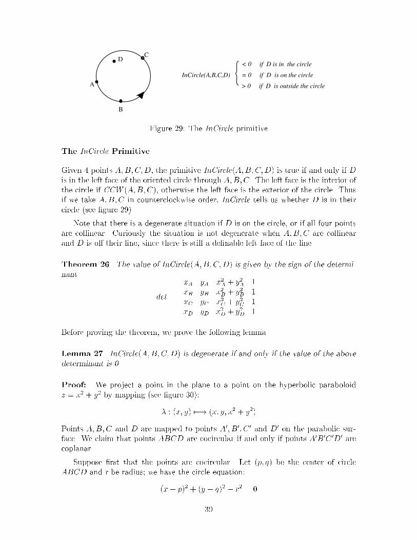
InCircle(A,B,C,D)

< 0 if D is in the circle

= 0 if D is on the circle

> 0 if D is outside the circle

Figure ��� The InCircle primitive

The InCircle Primitive

Given � points A�B�C�D� the primitive InCircle�A�B�C�D is true if and only if Dis in the left face of the oriented circle through A�B�C� The left face is the interior ofthe circle if CCW �A�B�C� otherwise the left face is the exterior of the circle� Thusif we take A�B�C in counterclockwise order� InCircle tells us whether D is in theircircle �see �gure ���

Note that there is a degenerate situation if D is on the circle� or if all four pointsare collinear� Curiously the situation is not degenerate when A�B�C are collinearand D is o� their line� since there is still a de�nable left face of the line�

Theorem ��� The value of InCircle�A�B�C�D is given by the sign of the determi�nant

det �

���������xA yA x�A � y�A �xB yB x�B � y�B �xC yC x�C � y�C �xD yD x�D � y�D �

���������Before proving the theorem� we prove the following lemma�

Lemma ��� InCircle�A�B�C�D is degenerate if and only if the value of the abovedeterminant is �

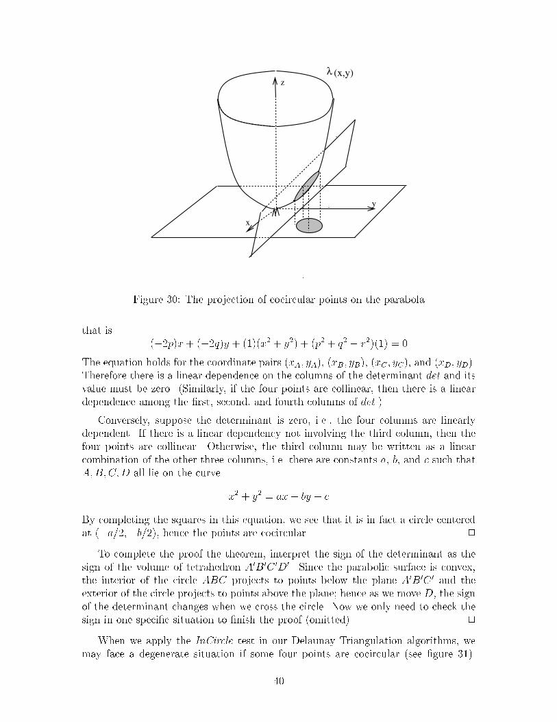
Proof� We project a point in the plane to a point on the hyperbolic paraboloidz � x� � y� by mapping �see �gure ���

� � �x� y ��� �x� y� x� � y�

Points A�B�C and D are mapped to points A�� B�� C � and D� on the parabolic sur�face� We claim that points ABCD are cocircular if and only if points A�B�C �D� arecoplanar�

Suppose �rst that the points are cocircular� Let �p� q be the center of circleABCD and r be radius� we have the circle equation�

�x� p� � �y � q� � r� � �

��

z

y

x

λ (x,y)

Figure ��� The projection of cocircular points on the parabola

that is���px � ���qy � ���x� � y� � �p� � q� � r��� � �

The equation holds for the coordinate pairs �xA� yA� �xB� yB� �xC � yC� and �xD� yD�Therefore there is a linear dependence on the columns of the determinant det and itsvalue must be zero� �Similarly� if the four points are collinear� then there is a lineardependence among the �rst� second� and fourth columns of det�

Conversely� suppose the determinant is zero� i�e�� the four columns are linearlydependent� If there is a linear dependency not involving the third column� then thefour points are collinear� Otherwise� the third column may be written as a linearcombination of the other three columns� i�e� there are constants a� b� and c such thatA�B�C�D all lie on the curve

x� � y� � ax � by � c

By completing the squares in this equation� we see that it is in fact a circle centeredat ��a����b��� hence the points are cocircular� �

To complete the proof the theorem� interpret the sign of the determinant as thesign of the volume of tetrahedron A�B�C �D�� Since the parabolic surface is convex�the interior of the circle ABC projects to points below the plane A�B�C � and theexterior of the circle projects to points above the plane� hence as we move D� the signof the determinant changes when we cross the circle� Now we only need to check thesign in one speci�c situation to �nish the proof �omitted� �

When we apply the InCircle test in our Delaunay Triangulation algorithms� wemay face a degenerate situation if some four points are cocircular �see �gure ���

��

OR

Figure ��� Two possible Delaunay edges for four cocircular points

L R

Figure ��� The structure of the cross edges

For simplicity when we present our algorithms we will assume that the points are ingeneral position� no three points are collinear and no four points are cocircular�

A Divide and Conquer Algorithm

In what follows�we present an algorithm to compute the Delaunay triangulation �andVoronoi diagram of n sites in the plane� and analyze its complexity� Suppose we haven sites in the plane S�� � � � � Sn� Sort them by x#coordinate �in case of equal x sortby y and then �as divide and conquer algorithms typically work divide them in twoequal halves� the left one �denoted by L and the right one �R� compute recursivelythe Delaunay diagrams of L and R� and then recombine� The recursion stops whenn � � or n � � since in these cases the diagram is easy �also our quad�edge structurecannot represent a single point � As usual the merge step needs to be analyzed inmore detail� During this step we have to delete some edges and add some others�Clearly we will delete some L#L �or R#R edges� and we will add only L#R �calledsometime cross edges� Indeed no new L#L �or R#R edge can be added� since suchedges would have already been Delaunay�

We can think of the cross edges ordered in ascending y#order and the algorithmthat we present will produce them in this order� The �rst cross edge will be the lowercommon tangent of the convex hull of L and the convex hull of R� similarly the last

��

L R

Figure ��� Finding the lower common tangent

cross edge will be their upper common tangent� Thus we can begin �nding the lowercommon tangent� To �nd it we use this algorithm�

�� Start from the edge e connecting the rightmost site of L with the leftmost siteof R�

�� While e is not a lower tangent to R� move its right endpoint counterclockwisearound the hull of R�

�� While e is not a lower tangent to L� move its left endpoint clockwise aroundthe hull of L�

�� If e is not yet the common lower tangent then go to step ��

This algorithm ends with the lower common tangent of L and R� and takes only lineartime �since it passes each hull edge at most once�

Lemma �� Any two consecutive cross edges share a common vertex�

Proof� Since the Delaunay diagram is a triangulation and the cross edges are ex�actly the Delaunay edges crossing a vertical line� two consecutive cross edges mustbelong to a triangular face and thus share a common vertex� �

A consequence of this lemma is that if we start from a known cross edge �let uscall it basel� its successor will be an edge going from one of the vertices of basel to aneighbor of the other vertex lying above basel� We can think of a circular bubble thathas basel as a chord and rises through that cord until it meets a new site� the edgeconnecting this site to the vertex of basel in the opposite half will be the next crossedge� This process continues until our bubble becomes the upper common tangent ofL and R �see �gure ���

��

Figure ��� The rising bubble

To �nd this edge� the following two lemmas are useful� Here Us�AB denotes theupper halfplane determined by AB� Ls�AB the lower halfplane� Hs�AB either ofupper or lower and Cir�XY Z denotes the interior of the circle through the threepoints X� Y� Z�

Lemma �� Let AB be an edge� For any point M and N� we always have Cir�ABMHs�AB � Cir�ABN Hs�AB or Cir�ABM Hs�AB � Cir�ABN Hs�AB

Proof� The proof is trivial and is omitted here� �

Lemma ��� Let AB be the basel edge and letNi i � �� � � � � k� be the L�neighbors of Ain Hs�AB in counterclockwise order� then the succession %i � Cir�ABNiHs�ABis unimodal in the sense that there is some j such that for � � i � j we have %i � %i��

while for j � i � k we have %i � %i���

Proof� For each circle ANiNi�� let Xi be its intersection with line AB� We claimthe sequence of points Xi move monotonically toward A� Consider � consecutiveneighbors Ni��� Ni� Ni�� of A� The point Ni�� is not inside the circle ANi��Ni� forotherwise ANi could not have been a Delaunay edge in L� Thus we have to pushcircle ANi��Ni through chord ANi to reach point Ni��� and the intersection with ABmoves toward A� proving our claim�

The lemma is now proved by observing that while Xi is to the right of B� B isinside the circle ANiNi�� or equivalently Ni�� is inside the circumcircle ABNi� so%i � %i��� After Xi moves to the left of B� a similar argument shows that Ni�� isoutside the circle ABNi� so %i � %i��� �

We can prove an analogous lemma for the R�neighbors of B� and in this way wecan �nd two candidates �one for each side to be the next cross edge� A �nal test

��

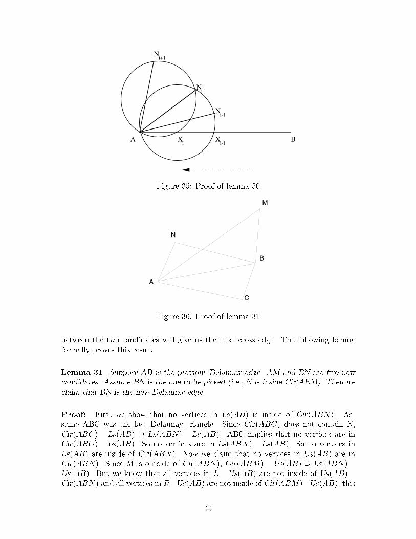
A B

N

Xi i-1

i+1

X

N

N

i

i-1

Figure ��� Proof of lemma ��

A

B

N

M

C

Figure ��� Proof of lemma ��

between the two candidates will give us the next cross edge� The following lemmaformally proves this result�

Lemma ��� Suppose AB is the previous Delaunay edge� AM and BN are two newcandidates� Assume BN is the one to be picked �i�e�� N is inside Cir�ABM�� Then weclaim that BN is the new Delaunay edge�

Proof� First we show that no vertices in Ls�AB is inside of Cir�ABN� As�sume ABC was the last Delaunay triangle� Since Cir�ABC does not contain N�Cir�ABC Ls�AB � Ls�ABN Ls�AB� ABC implies that no vertices are inCir�ABC Ls�AB� So no vertices are in Ls�ABN Ls�AB� So no vertices inLs�AB are inside of Cir�ABN� Now we claim that no vertices in Us�AB are inCir�ABN� Since M is outside of Cir�ABN� Cir�ABM Us�AB � Ls�ABN Us�AB� But we know that all vertices in L Us�AB are not inside of Us�AB Cir�ABN and all vertices in RUs�AB are not inside of Cir�ABMUs�AB� this

��

implies that all vertices in Us�AB are not in Ls�ABN Us�AB� This completesthe proof� �

Now we are going to analyze the time complexity for the algorithm� Suppose A scandidate is Nj� The unimodularity proved in the lemma allows us to �nd Nj inj comparisons� by searching until the �rst �local minimum� going counterclockwisearound A� Furthermore the edges ANi for i � j can be immediately deleted �even ifB s candidate won over Nj because we know that these edges cannot be part of themerged Delaunay diagram �B prevents them�

Thus the cost of searching through the candidate vertices can be charged to thedeleted edges �all other costs are clearly linear� Since the old triangulations had alinear number of edges� this gives us linear time overall to �nd all the cross edges�completing the merge� Since the �rst part of the merge ��nding the lower commontangent was also linear time� the entire merge process takes O�n time� and the timecomplexity of the algorithm is O�n log n �Note that the initial sorting step needs tobe done only once�

� Randomized Incremental Algorithm for Delau�

nay Triangulations

In the previous lecture we discussed a divide�and�conquer algorithm to �nd the Delau�nay triangulation of a set of sites� In this lecture we present a randomized incrementalalgorithm for the same problem� We will �rst discuss the basic incremental algorithm�without introducing randomization� We will then randomize the algorithm to im�prove its expected running time�

A Basic Incremental Algorithm

The idea in our incremental method is to add the sites in some sequence to the currentset and update the Delaunay triangulation of the set of sites to re�ect the addition ofthe new site� For convenience in describing the algorithm� we add three hypotheticalsites at the very beginning� they are chosen such that they form a very large trianglethat contains all the other sites� If we make this triangle large enough� it will clearlynot a�ect the Delaunay triangulation of the original sites�

We now de�ne our incremental Delaunay triangulation algorithm� starting withthe triangle on these three sites� adding the other sites in some order� and updatingthe Delaunay triangulation after each addition�

Suppose that we add a new site S� Assuming non�degeneracies� it will be insidea triangle� The idea is to locate the triangle that the new site falls into� link the newsite to the three vertices of the enclosing triangle� and reconsider the Delaunayhoodof the edges of the enclosing triangle� if such an edge fails the circle test� the edge is

��

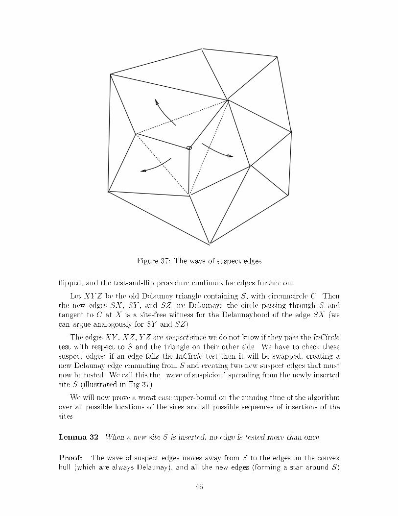
Figure �� The wave of suspect edges

�ipped� and the test�and��ip procedure continues for edges further out�

Let XY Z be the old Delaunay triangle containing S� with circumcircle C� Thenthe new edges SX� SY � and SZ are Delaunay� the circle passing through S andtangent to C at X is a site�free witness for the Delaunayhood of the edge SX �wecan argue analogously for SY and SZ�

The edges XY � XZ� Y Z are suspect since we do not know if they pass the InCircletest with respect to S and the triangle on their other side� We have to check thesesuspect edges� if an edge fails the InCircle test then it will be swapped� creating anew Delaunay edge emanating from S and creating two new suspect edges that mustnow be tested� We call this the �wave of suspicion� spreading from the newly insertedsite S �illustrated in Fig ��

We will now prove a worst case upper�bound on the running time of the algorithmover all possible locations of the sites and all possible sequences of insertions of thesites�

Lemma ��� When a new site S is inserted� no edge is tested more than once�

Proof� The wave of suspect edges moves away from S to the edges on the convexhull �which are always Delaunay� and all the new edges �forming a star around S

��

are never suspect� �

When the wave stops all the edges pass the InCircle test� so the triangulation isagain Delaunay� The previous lemma tells us that each insertion needs at most O�ntime� so the total time required by the algorithm is O�n��

It is possible to construct example input sequences which achieve this quadraticrunning time �we leave that as an exercise� We will now see that this algorithm hasmuch better O�n lgn expected running time when the input sites are inserted in arandom order�

Randomizing the Incremental Method

We saw that the obvious sequential incremental method may create O�n� Delaunaytriangles during the running of the algorithm� To try to achieve O�n logn time weneed to randomize� The algorithm is very easy� Given a set of sites� we simply choosea random ordering of the sites and add them one at a time� updating the Delaunaytriangulation as already described� Note that we have not yet described a way oflocating the triangle in which the new site lies �we will do this in the next section�

We observe that the total amount of work performed during the algorithm isrelated to the number of Delaunay triangles that ever arise during the running of thealgorithm� We will prove that the expected number of such triangles is ��n�

Theorem ��� If is the expected number of Delaunay triangles that ever ariseduring the running of the algorithm� then � O�n� In fact� � �n� ��Hn � �����where Hn � � � �

�� �

�� � � �� �

n�

Proof� For a triangle de�ned by three sites� let w� denote the scope of thetriangle� the number of sites inside the circumcircle of � Let Tj be the number oftriangles of scope j �so in particular T� is the number of triangles in the �nal Delaunaytriangulation� Then

�X�

Pr�at some point of the algorithm� appears as Delaunay�

If w� � j� then appears as Delaunay sometime during the algorithm i� the threesites de�ning are chosen before any of the j sites inside its circumcircle� Thus

Pr� appears as Delaunay� �� j

�j � � �

�

�j � ��j � ��j � �

and

�n��Xj�

�

�j � ��j � ��j � �Tj

Now� suppose we choose r of the sites at random and look at the Delaunay triangula�tion of this r�set� The expected number of triangles in this triangulation is �r�hr���

�

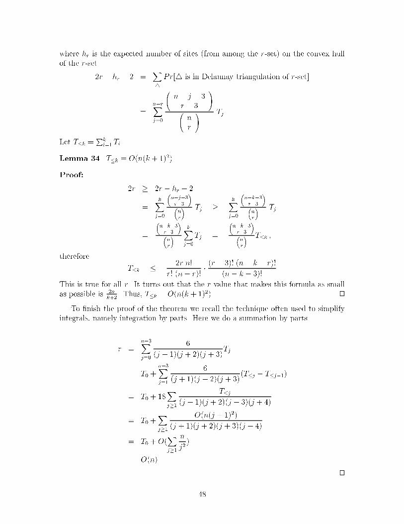
where hr is the expected number of sites �from among the r�set on the convex hullof the r�set�

�r � hr � � �X�

Pr� is in Delaunay triangulation of r�set�

�n�rXj�

n� j � �r � �

nr

Tj

Let T�k �Pk

i� Ti�

Lemma ��� T�k � O�n�k � ���

Proof�

�r � �r � hr � �

�kX

j�

�n�j��r��

��nr

� Tj �kX

j�

�n�k��r��

��nr

� Tj

�

�n�k��r��

��nr

� kXj�

Tj �

�n�k��r��

��nr

� T�k �

therefore

T�k � �r n

r �n� r � �r � � �n� k � r

�n� k � �

This is true for all r� It turns out that the r value that makes this formula as smallas possible is �n

k��� Thus� T�k � O�n�k � ��� �

To �nish the proof of the theorem we recall the technique often used to simplifyintegrals� namely integration by parts� Here we do a summation by parts�

�n��Xj�

�

�j � ��j � ��j � �Tj

� T� �n��Xj�

�

�j � ��j � ��j � ��T�j � T�j��

� T� � ��Xj��

T�j�j � ��j � ��j � ��j � �

� T� �Xj��

O�n�j � ��

�j � ��j � ��j � ��j � �

� T� � O�Xj��

n

j�

� O�n

�

��

E�cient Randomized Point�Location

While insertion of a particular site can take O�n time in the worst case� we showedthat if sites are inserted in random order� the expected overall running time of theupdate part of the incremental algorithm for constructing the Delaunay triangula�tion is O�n� We are yet to describe a crucial part of our randomized incrementalalgorithm� namely� locating the triangle in which the new site falls�

In order to obtain an overall e�cient algorithm for the randomized incrementalconstruction of the Delaunay triangulation� we need an e�cient algorithm for locatingthe triangle that contains a new site� We will give an algorithm for this point�locationproblem that contributes an overall randomized time complexity of O�n logn� result�ing in an overall randomized time complexity of O�n logn� This bound is optimal�since sorting is O�n reducible to computing the Delaunay triangulation� and sortingis known to have a lower bound of ��n log n in the randomized time complexitymodel�

The trick to achieving an e�cient algorithm for the point�location problem is tokeep a history of the construction of the triangulation� We can think of this historyas consisting of a stack of paper triangles glued on top of one another�

Given a history of the construction� the algorithm for �nding the triangle in thecurrent triangulation containing a query point P is as follows� Assume we know thatthe triangle T contains point P at some step in the construction of the triangulation�If T is present in the �nal triangulation� we are done� Otherwise� T will be split inone of two ways� either a new point of the triangulation is added into the triangle T �in which case T will be split into three children� or one of the edges of T gets �ipped�in which case T will be split into two children �see Figure ��� In both cases� it takesonly constant time to determine which �child� of T contains the query point P �

In order to prove that the overall running time of the point�location part of thealgorithm for the incremental construction of the Delaunay triangulation is O�n lognon the average� we need to obtain a bound on the number of triangles examined duringeach of the point�locations� In the �stack of paper triangles metaphor�� we need toestimate the average thickness of the stack of paper triangles that are glued on topof one another at each site�

Lemma ���nXi�

E�& of triangles crossed during the i�th insertion � O�n logn

Note that this lemma does not establish that any speci�c point�location query can becarried out in expected time O�logn �why��

Proof� We will carry out an amortized analysis� We will relate the number oftriangles crossed during the search to the number Tj of triangles of scope j �rememberthat the scope of a triangle is the number of sites contained in the circumcircle ofthat triangle�

��

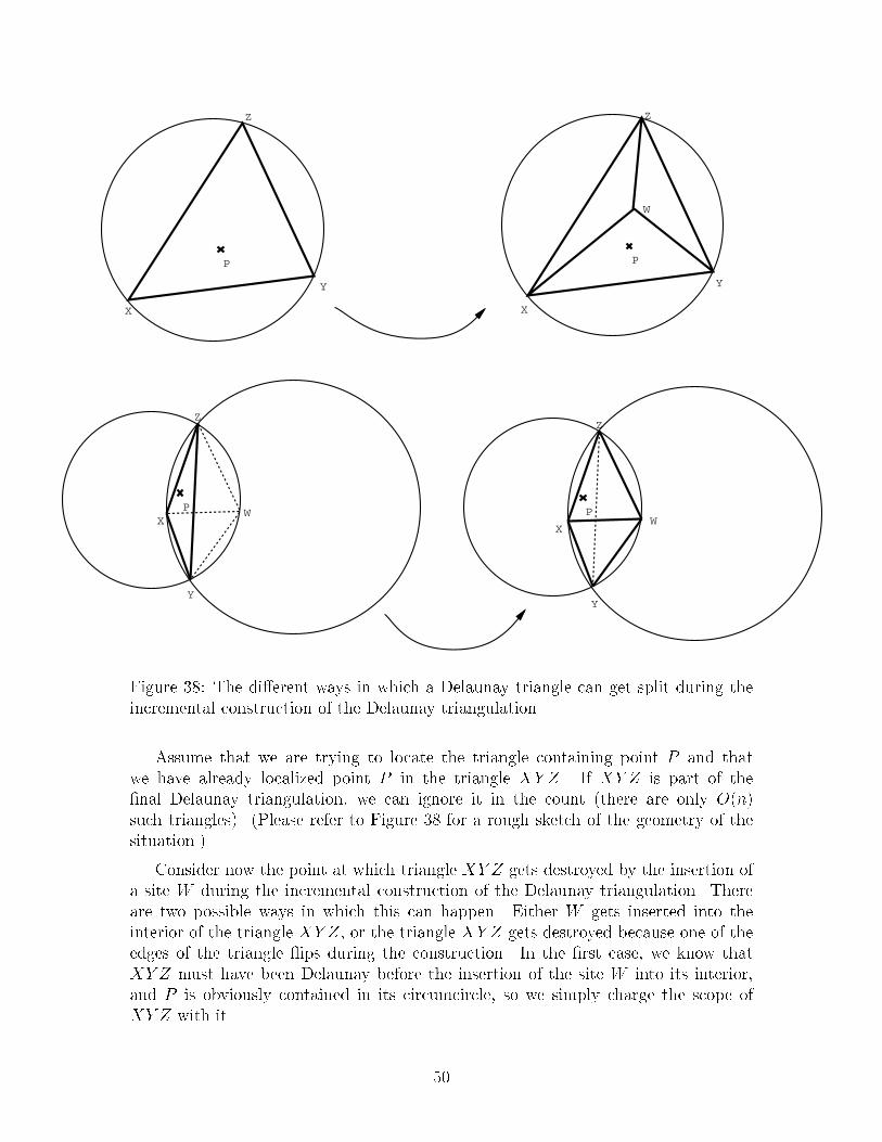
P P

P P

W

WWX

Y

Z

X

Y

Z

X

Y

Z

X

Y

Z

Figure ��� The di�erent ways in which a Delaunay triangle can get split during theincremental construction of the Delaunay triangulation�

Assume that we are trying to locate the triangle containing point P and thatwe have already localized point P in the triangle XY Z� If XY Z is part of the�nal Delaunay triangulation� we can ignore it in the count �there are only O�nsuch triangles� �Please refer to Figure �� for a rough sketch of the geometry of thesituation�

Consider now the point at which triangle XY Z gets destroyed by the insertion ofa site W during the incremental construction of the Delaunay triangulation� Thereare two possible ways in which this can happen� Either W gets inserted into theinterior of the triangle XY Z� or the triangle XY Z gets destroyed because one of theedges of the triangle �ips during the construction� In the �rst case� we know thatXY Z must have been Delaunay before the insertion of the site W into its interior�and P is obviously contained in its circumcircle� so we simply charge the scope ofXY Z with it�

��

In the second case� let XW be the edge that replaces Y Z� Now� depending onwhich way the �wave of suspect edges� has arrived at the edge Y Z� either XY Z orWYZ was Delaunay before the �ip� If XY Z was Delaunay� we can again simplycharge P to its scope� If WYZ was Delaunay before the �ip� the evidence against itsDelaunayhood must have come from site X� But if X is contained in the circumcircleof WYZ� so is P � and we can charge P against the scope of the Delaunay triangleWYZ�

Therefore� we can charge every crossing to an event of the form that P is con�tained in the circumcircle of a triangle that was Delaunay at some point during theconstruction� And� if P charges the circumcircle of some triangle� it is easy to seethat it can do so only once�

Therefore� we obtain�

nXi�

E�& of triangles crossed during the ith insertion

� E�X

scopes of all Delaunay triangles that ever arose

� E�n��Xj�

j Tj�j � ��j � ��j � �

This last expression is easily seen to be O�n logn�we use the same techniquewe used for obtaining the O�n bound on the number of triangles formed during theconstruction� Roughly� the above expression is of the form

Pn Tjj�

� if we consider thenumber T�j of triangles of scope less than or equal to j� this sum can be rewritten

to be roughly of the formPn T�j

j�� Using our previous results for T�j� this expression

takes on the formPn nj�

j�� n

Pn �j

� O�n logn� �

With this lemma� and the above observation about the cost of locating subtrian�gles� we can therefore state the following theorem�

Theorem ��� The expected overall cost of point�location for the randomized incre�mental construction of the Delaunay triangulation is O�n logn�

Convex Hulls and Delaunay Triangulations

In the previous lecture we introduced a correspondence between the sites of ��space topoints on a paraboloid in ��dimensions such that the mapping satis�es some specialproperties� Recall that we project a point in the plane to a point on the hyperbolicparaboloid z � x� � y� by mapping �see �gure ���

� � �x� y ��� �x� y� x� � y�

Points A�B�C and D are mapped to points A�� B�� C � and D� on the parabolic surface�We proved that points ABCD are cocircular if and only if points A�B�C �D� arecoplanar�

��

z

y

x

λ (x,y)

Figure ��� The projection of cocircular points on the parabola

This implies that every circle in the plane maps to a planar curve on the paraboloid�the intersection of some plane with the paraboloid�

Our construction has another nice property� Suppose we are given a triangleformed by three sites in the plane� which maps to three points on the paraboloid�From our construction� it easily follows that a fourth site lies inside the circle formedby the three sites in the plane i� the mapped point lies below the plane formed bythe three points in ��space� This means that Delaunay triangles in the plane �whosecircumcircles are empty map to triangles in ��space which don t have any point belowthem� In other words� a Delaunay triangle maps to a lower convex hull triangle ofthe mapped set of points in ��space�

Hence� the problem of �nding the Delaunay Triangulation of a set of points reducesto that of �nding the lower convex hull of a set of points on a paraboloid in threedimensions� It turns out that this correspondence extends to arbitrary dimensions�That is� the problem of �nding the Delaunay diagram of n points in d dimensionscorresponds to the problem of �nding the convex hull of n points in d� � dimensions�We do not prove this claim here� although it is very straightforward�

Applications

Computing the Voronoi diagram and Delaunay triangulation is useful not only for itsown sake� but also is an important part of many other e�cient geometric algorithms�

For example� the edge connecting the closest pair of sites in a collection of sitesis a Delaunay edge� Finding the closest pair is therefore reducible to �nding the

��

minimum length Delaunay edge�

Finding all nearest neighbors is similarly easily accomplished starting with theDelaunay triangulation� because all edges connecting a site and its nearest neighbormust be Delaunay�

As a �nal example consider the computation of the Euclidean Minimum SpanningTree �EMST� The EMST must be a subset of the Delaunay triangulation �consideredas a graph� and can be obtained from it by application of a minimum spanningtree �MST graph algorithm� In fact� all the known EMST algorithms with goodcomplexity compute the Delaunay triangulation �rst�

Acknowledgements� The author wishes to thank the following students whosescribed notes were used in preparing this writeup� Zhenyu Li �Harvard� MichelangeloGrigni� Mark Day� Rosario Gennaro� Dina Kravets� Thomas Breuel� Songmin Kim�Alex Ishii� Mark Smith �MIT� Alan Hu� Eric Rose� Eric Veach� David Karger� DanYang� G�D� Ramkumar �Stanford� and Ken Stanley who scribed a lecture of RaimundSeidel �Berkeley�

Bibliography

References

�ASS��� Pankaj Agarwal� Micha Sharir� and Peter Shor� Sharp upper and lowerbounds on the length of general Davenport#Schinzel sequences� Journalof Combinatorial Theory Series A� ������#��� �����

Shows ���n � ��n ����n�� as well as near�tight bounds for higher s� �s�n

� n����n��b�s�����c�o���

where the o�� goes to zero with large n �but not s�

�CGL��� Bernard Chazelle� Leonidas Guibas� and D� Lee� The power of geometricduality� BIT� ����#��� �����

As an application of geometric duality� this paper gives an optimalO�logn�k algorithm for the problem of half�planar queries in the plane�Here n is the total number of points� and k the size of the desired an�swer� Unfortunately the methods of this paper seem to work only in twodimensions�

�Dav�� H� Davenport� A combinatorial problem connected with di�erential equa�tions II� Acta Arithmetica� �����#��� ����

Shows ��� o��n � ���n � O�n logn� log log n�

�Del��� B� Delaunay� Sur la sph'ere vide� Izvestia Akademii Nauk SSSR� VII Seria�Otdelenie Matematicheskii i Estestvennyka Nauk� �����#���� October����� English translation manuscript by M� Dillencourt�

��

�DS��� H� Davenport and A� Schinzel� A combinatorial problem connected withdi�erential equations� American Journal of Mathematics� �����#���������

Source of the Davenport#Schinzel sequence problem� Solves the s � �cases� shows �s�n � �s��n�n����� �n�O�� � ���n � �n���lnn�

and �s�n � n�O�p

s log s log n��

�Ede�� Herbert Edelsbrunner� Algorithms in Combinatorial Geometry� Springer�Verlag� ����

An advanced topical reference work�

�EG��� Herbert Edelsbrunner and Leonidas Guibas� Topologically sweeping an ar�rangement� Journal of Computer and System Sciences� ������#���� �����

This paper shows how a �topological line� can be used to sweep over aline arrangement in O�n� time with O�n working storage�

�GKS��� Leonidas Guibas� Donald Knuth� and Micha Sharir� Randomized incre�mental construction of delaunay and voronoi diagrams� In M� S� Paterson�editor� Automata� Languages and Programming� �� th International Collo�quium� volume ��� of Lecture Notes in Computer Science� Springer�Verlag������ To appear in Algorithmica�

This paper shows that incremental techniques work very well for the con�struction of Voronoi!Delaunay diagrams� if one �rst randomizes the se�quence of insertions of the de�ning points� The paper also shows how thehistory of the data�structure thus constructed can be kept around so as toaid the location of future points in the structure�

�GS��� Leonidas Guibas and Jorge Stol�� Primitives for the manipulation of gen�eral subdivisions and the computation of voronoi diagrams� ACM Trans�actions on Graphics� �����#���� April �����

This paper is really about the quad�edge data structure for representingsubdivisions of two�dimensional manifolds� The authors give a mathemati�cally rigorous development of the data structure and prove its �topologicalcompleteness�� As an afterthought� they also show how to use it to imple�ment e�cient Voronoi!Delaunay algorithms in the plane using only a fewgeometric and topological primitives�

�GS�� Leonidas Guibas and Jorge Stol�� Ruler� compass� and computer� thedesign and analysis of geometric algorithms� In R� A� Earnshaw� editor�Theoretical Foundations of Computer Graphics and CAD� pages ���#����Springer�Verlag� ����

This is a survey paper trying to illustrate each of the major techniques inComputational Geometry as of ��� with a worked out example�

��

�HS��� S� Hart and Micha Sharir� Nonlinearity of Davenport#Schinzel sequencesand of generalized path compression schemes� Combinatorica� �����#�������

Shows ���n � ��n��n�

�Meh��� Kurt Mehlhorn� Data Structures and Algorithms � Multi�dimensionalSearching and Computational Geometry� EATCS Monographs on Theo�retical Computer Science� Springer�Verlag� �����

One of the �rst texts on computational geometry� the third of three vol�umes by Mehlhorn�

�PS��� Franco P� Preparata and Michael Ian Shamos� Computational Geometry�Texts and Monographs in Computer Science� Springer�Verlag� �����

A good elementary introduction�

�Sha�� Micha Sharir� Almost linear upper bounds on the length of generalDavenport#Schinzel sequences� Combinatorica� ����#���� ����

Shows �s�n � O�n��nO���n�s����

�Sha��� Micha Sharir� Improved lower bounds on the length of Davenport#Schinzelsequences� Combinatorica� ����#���� �����

Shows ��s���n � ��n�s�n� by an inductive construction based on thatof �HS����

�Sze�� Endre Szemer(edi� On a problem of Davenport and Schinzel� Acta Arith�metica� ������#���� ����

Shows �s�n � Csn log� n� where Cs depends only on s� Di�cult�

�vL��� Jan van Leeuwen� editor� Handbook of Theoretical Computer Science� El�sevier and MIT Press� �����

�Yao��� F� Frances Yao� Computational geometry� In Jan van Leeuwen� editor�Handbook of Theoretical Computer Science� volume A� chapter � pages���#���� Elsevier and MIT Press� �����

An excellent recent survey of the �eld� including an extensive bibliography�

��