Barrier Option Pricing by Branching Processes Georgi K. Mitov ∗ Svetlozar T. Rachev † Young Shin Kim Frank J. Fabozzi Georgi K. Mitov Institute of Mathematics and Informatics, Bulgarian Academy of Science ”Acad. G. Bonchev” Str., Bl. 8, 1113, Sofia, Bulgaria and Senior Quant, FinAnalytica Inc. E-mail: georgi.mitov@finanalytica.com Svetlozar T. Rachev Chair-Professor, Chair of Statistics, Econometrics and Mathematical Finance, School of Economics and Business Engineering, University of Karlsruhe and KIT, Kollegium am Schloss, Bau II, 20.12, R210, Postfach 6980, D-76128, Karlsruhe, Germany and Department of Statistics and Applied Probability, University of California, Santa Barbara, and Chief-Scientist, FinAnalytica Inc. E-mail: [email protected] Young Shin Kim Department of Statistics, Econometrics and Mathematical Finance, School of Economics and Business Engineering, University of Karlsruhe and KIT Kollegium am Schloss, Bau II, 20.12, R210, Postfach 6980, D-76128, Karlsruhe, Germany E-mail: [email protected] Frank J. Fabozzi Professor in the Practice of Finance, Yale School of Management, 135 Prospect Street, Box 208200, New Haven, CT 06520-8200, USA E-mail: [email protected] * Georgi Mitov is supported by the German Academic Exchange Service (DAAD) and in part by NSF- Bulgaria (grant VU-MI-105/20-05). † Svetlozar Rachev gratefully acknowledges research support by grants from Division of Mathematical, Life and Physical Sciences, College of Letters and Science, University of California, Santa Barbara, the Deutschen Forschungsgemeinschaft, and the Deutscher Akademischer Austausch Dienst. 1

Welcome message from author
This document is posted to help you gain knowledge. Please leave a comment to let me know what you think about it! Share it to your friends and learn new things together.
Transcript

Barrier Option Pricing by Branching Processes
Georgi K. Mitov∗ Svetlozar T. Rachev†
Young Shin Kim Frank J. Fabozzi
Georgi K. Mitov
Institute of Mathematics and Informatics, Bulgarian Academy of Science”Acad. G. Bonchev” Str., Bl. 8, 1113, Sofia, Bulgariaand Senior Quant, FinAnalytica Inc.E-mail: [email protected]
Svetlozar T. Rachev
Chair-Professor, Chair of Statistics, Econometrics and Mathematical Finance, School ofEconomics and Business Engineering, University of Karlsruhe and KIT, Kollegium amSchloss, Bau II, 20.12, R210, Postfach 6980, D-76128, Karlsruhe, Germanyand Department of Statistics and Applied Probability, University of California, SantaBarbara,and Chief-Scientist, FinAnalytica Inc.E-mail: [email protected]
Young Shin Kim
Department of Statistics, Econometrics and Mathematical Finance, School of Economicsand Business Engineering, University of Karlsruhe and KITKollegium am Schloss, Bau II, 20.12, R210, Postfach 6980, D-76128, Karlsruhe, GermanyE-mail: [email protected]
Frank J. Fabozzi
Professor in the Practice of Finance,Yale School of Management,135 Prospect Street, Box 208200,New Haven, CT 06520-8200, USAE-mail: [email protected]
∗Georgi Mitov is supported by the German Academic Exchange Service (DAAD) and in part byNSF- Bulgaria (grant VU-MI-105/20-05).
†Svetlozar Rachev gratefully acknowledges research support by grants from Division of Mathematical,Life and Physical Sciences, College of Letters and Science, University of California, Santa Barbara, theDeutschen Forschungsgemeinschaft, and the Deutscher Akademischer Austausch Dienst.
1

Barrier Option Pricing by Branching Processes
Abstract
This paper examines the pricing of barrier options when the price of the un-derlying asset is modeled by branching process in random environment (BPRE).We derive an analytical formula for the price of an up-and-out call option, oneform of a barrier option. Calibration of the model parameters is performed usingmarket prices of standard call options. Our results show that the prices of bar-rier options that are priced with the BPRE model deviate significantly from thosemodeled assuming a lognormal process, despite the fact that for standard options,the corresponding differences between the two models are relatively small.
Key words: Barrier option, up-and-out call option, Bienayme-Galton-Watsonbranching process, branching process in random environment
2

1 Introduction
Barrier options, also known as knock-in options or knock-out options, have become
increasingly popular since they were first traded in the over-the-counter (OTC) market
in 1967. Their popularity resulted in the introduction of barrier options on exchanges
by 1991, first by the Chicago Board Option Exchange and then by the American Stock
Exchange. The appealing feature of this exotic option product is twofold. First, it
provides an investor with flexibility in a number of hedging strategies. Second, it is less
expensive than standard options.
Barrier options are a type of path-dependent option which include down-and-out op-
tions, down-and-in options, up-and-out options, and up-and-in options. In 1973, Merton
[20] provided a closed-form solution for down-and-out call options. Since then, closed-
form solutions for many European barrier options have been developed by Reiner and
Rubinstein [23], Kunitomo and Ikeda [15], Carr [8], and Geman and Yor [14]. Numerical
methods have been proposed to handle American or other more complex barrier options
by Boyle and Lau [4], Ritchken [25] , Broadie, Glasserman, and Kou [7], Boyle and Tian
[6], and Zvan, Vetzal and Forsyth [31]. Most of the published papers on barrier options
assume the underlying asset follows geometric Brownian motion. This implies that the
price of the underlying asset is log-normally distributed as in the Black-Scholes [3] model.
This assumption has several drawbacks.
The first drawback is that stock prices on the New York Stock Exchange (NYSE)
were quoted in units of $1/8, then in $1/16, and now $0.01. This discreteness of the
stock price contradicts the continuous distribution assumption in the Black-Scholes for-
mula. Second, it is evident that stock prices sometimes exhibit large jumps when some
important news is disclosed. Third, extensive empirical evidence, pioneered by Mandel-
brot [18, 19] and Fama [13], empirically documented that the logarithm of stock returns
tend to be leptokurtic; that is, their distributions have thicker tails than the normal
distribution derived from the geometric Brownian motion law. Furthermore, Black [2]
noted the so-called “leverage effect,” meaning that the volatility of stock returns tends
to be negatively correlated with the price.
There are different ways to avoid these drawbacks of the lognormal model. One of
3

them is to model the price of the underlying asset using different stochastic processes
which possess some of the stylized facts reported for stock prices. Thus, Zhou [30]
examines the case where the stock price follows a jump diffusion process. Valuation
of barrier options in a constant elasticity of variance (CEV) model is treated in Boyle
and Tian [5] and Davydov and Linetsky [10]. Shoutens and Symens [27] utilize Levy
stochastic volatility models to price barrier options. Riberio and Webber [24] present a
Monte Carlo algorithm for pricing barrier options with the variance gamma (VG) model.
In the present paper, we use a branching process in a random environment (BPRE)
to model the stock price. This model of stock price movement was introduced by Epps
[11] in 1996. The model, constructed by Bienayme-Galton-Watson branching process
subordinated with a Poisson process, captures the stylized facts about stock return dis-
tributions. Specifically, the return distribution exhibits thick tails and a variance that
decreases with the level of the stock price. The process also allows for possible jumps
in stock prices, and takes into account the possibility of bankruptcy, something that is
neglected in many other models.
Williams [29] provides an exact formula for the price of a European put option based
on the BPRE model. Liu [17] applies the BPRE model to options on a sample of indi-
vidual U.S. equities. Inferring the parameters from transaction prices of traded options,
Liu finds that for the in-sample prediction, the model typically eliminates the smile effect
that has been observed for option prices. The results are mixed when out-of-sample pre-
dictions are compared with the ad hoc version of Black-Scholes with moneyness-specific
implicit volatilities. Liu does find evidence that the predictions are better for options on
low-priced stocks, where the discreteness arising from the minimum tick size would seem
to be more relevant.
In this paper, we derive a formula for the price of an up-and-out call option based
on BPRE and compare the results with the prices based on the lognormal model. The
paper is organized as follows. In Section 2, we review the mathematical definition of the
BPRE model and its main properties and advantages. Since we rely on a methodology
for the pricing of a European call option formulated by Mitov and Mitov [21] for the
calibration of the equivalent martingale measure (EMM) parameters, we provide the
4

formula at the end of Section 2. The formula for the price of an up-and-out call option
is derived in Section 3. In Section 4, we report numerical results for barrier options on
several stocks and the S&P 500 index. We calibrate both BPRE and lognormal models
to market prices of standard options, and subsequently price up-and-out call options.
We then compare those prices based on the BPRE model and lognormal model. Section
5 summarizes our findings.
2 The Model
2.1 Branching Processes
Let us consider a Bienayme-Galton-Watson branching process, Zn, n = 0, 1, 2, . . .
with a non-random number of ancestors Z0 > 0, and the offspring probability distribution
P(Zn+1 = 0|Zn = 1) = (1 − a),
P(Zn+1 = k|Zn = 1) = ap(1 − p)k−1, k = 1, 2, . . . ,
0 < a < 1, 0 < p < 1.
The probability generating function (p.g.f.) f(s) = E[sZ1|Z0 = 1] of the offspring
distribution can be easily represented in terms of the distribution’s factorial moments by
f(s) = 1 − m(1 − s)
1 +b
2m(1 − s)
, s ∈ [0, 1],
where m = a/p is the offspring mean and
b = 21 − p
pm, σ2 = b + m − m2 =
a
p
(
(1 − p) + (1 − a)
p
)
are the offspring second moment and the offspring variance.
Such a function has fractional linear form. It is well known (see e.g. Sevastyanov
[26]) that for the p.g.f. fn(s) = E[sZn|Z0 = 1], the following relation holds
(1) fn(s) = 1 − mn(1 − s)
1 +b
2m
1 − mn
1 − m(1 − s)
.
In Section 3, we will need the probabilities
P(Zn = k|Z0 = 1), k = 0, 1, 2, . . . , n = 1, 2, . . . .
5

Differentiating (1), we obtain
(2) f ′n(s) =
mn
[
1 +b(1 − mn)
2m(1 − m)(1 − s)
]2 ,
and for k = 2, 3, . . . ,
(3) f (k)n (s) =
k!mn
[
b(1 − mn)
2m(1 − m)
]k−1
[
1 +b(1 − mn)
2m(1 − m)(1 − s)
]k+1.
From the properties of the p.g.f., it follows that
P(Zn = k|Z0 = 1) =f
(k)n (0)
k!,
therefore we get for k = 1, 2, . . .
(4) P(Zn = k|Z0 = 1) =
mn
[
b(1 − mn)
2m(1 − m)
]k−1
[
1 +b(1 − mn)
2m(1 − m)
]k+1.
Then the probability for extinction in the n−th generation is
(5) P(Zn = 0|Z0 = 1) = 1 −∞
∑
k=1
mn
[
b(1 − mn)
2m(1 − m)
]k−1
[
1 +b(1 − mn)
2m(1 − m)
]k+1
= 1 − mn
1 +b(1 − mn)
2m(1 − m)
.
Substituting s = 1 in (2), we get the first moment of the process
(6) E[Zn|Z0 = 1] =
mn, m 6= 1,1, m = 1.
Substituting k = 2 and s = 1 in (3), we obtain the second factorial moment
(7) E[Zn(Zn − 1)|Z0 = 1] =
bmn−1 1 − mn
1 − m, m 6= 1,
bn, m = 1.
If the process starts with Z0 = I > 1 number of ancestors, it is a sum of I independent
and identically distributed branching processes, each of them beginning with an ancestor.
Therefore,
E[sZn|Z0 = I] = (fn(s))I
6

and we can calculate for k = 1, 2, . . .
P(Zn = k|Z0 = I) =dk(fn(s))I
dsk
∣
∣
∣
∣
s=0
.
Instead of using the derivatives, we suggest the following simple iterative procedure.
For any n > 0, Z0 = I > 1, and K ≥ 0, calculate:
(i) P(Zn = k|Z0 = 1) for k = 0, 1, 2, . . . , K by (4) and (5).
(ii) For Z0 = 2, the process is the sum of two independent processes each of which
begins with Z0 = 1 particle. Therefore,
P(Zn = k|Z0 = 2) =k
∑
j=0
P(Zn = j|Z0 = 1)P(Zn = k − j|Z0 = 1),
for all k = 0, 1, 2, . . . , K.
(iii) For Z0 = I, I ≥ 3, the process is the sum of two independent processes one of
which starts with Z0 = I − 1 and the other starts with Z0 = 1 particle. That is,
P(Zn = k|Z0 = I) =k
∑
j=0
P(Zn = j|Z0 = I − 1)P(Zn = k − j|Z0 = 1).
for all k = 0, 1, 2, . . . , K.
Note that the calculations can be easily performed using numerical software if for
a fixed n and K, the probabilities p1k(n) = P(Zn = k|Z0 = 1), k = 0, 1, 2, . . . , K,
calculated in the point (i) are entered in an upper triangular matrix as follows
P(n) =
p10(n) p11(n) p12(n) . . . p1K(n)0 p10(n) p11(n) . . . p1,K−1(n)0 0 p10(n) . . . p1,K−2(n). . . . . . . . . . . . . . .0 0 0 . . . p10(n)
.
It is not difficult to see that the probabilities pIk(n) = P(Zn = k|Z0 = I), k =
0, 1, 2 . . . , K are equal to the (1, k)−th element of the I−th power of matrix P(n).
2.2 Branching process in random environment as a price pro-
cess
Assume now that on the common probability space (Ω,A, P) are given (i) a super-
critical (m > 1) Bienayme-Galton-Watson branching process Zn, n = 0, 1, 2, . . . defined
in the previous section and (ii) an independent of it Poisson process N(t), t ≥ 0 with
7

intensity λ > 0. Following Epps [11] or [12], define the randomly indexed branching
process, which is in fact a branching process in random environment (BPRE),
S(t) = ZN(t), t ≥ 0.
Here S(t) represents the price of one share of stock at time t measured in units of mini-
mum price movements (for example $0.01). Equity prices are then viewed as consisting
of an integer number of “price particles.” In each period, each “price particle” of equity
price produces a random number of offspring “price particles,” the aggregate number
of which comprises the equity price in the next period. Hence, by allowing a random
number of generations to occur in each period, the BPRE model generates prices in
continuous time.
The independence of Zn and N(t) yields the following formula for the p.g.f. of the
process S(t) = ZN(t), starting with Z0 ≡ S(0) ≥ 1 ancestors
Φ(t, s) =∞
∑
n=0
(λt)n
n!e−λt (fn(s))S(0)
=∞
∑
n=0
(λt)n
n!e−λt
1 − mn(1 − s)
1 +b
2m
1 − mn
1 − m(1 − s)
S(0)
.
Using the p.g.f. and formulas (6) and (7), after some calculations we derive the following
formulas for the mean and the variance of the process S(t)
(8) M(t) = E[S(t)|S(0)] =
S(0)eλt(m−1), m 6= 1,S(0), m = 1,
σ2(t) = V ar[S(t)|S(0)] =
S(0)2[eλt(m2−1) − e2λt(m−1)]
+S(0)σ2[eλt(m2−1) − eλt(m−1)]
m(m − 1), m 6= 1
S(0)σ2λt, m = 1.
These formulas allow us to examine in detail some of the main properties of the total
return R(t) = [S(t)−S(0)]/S(0) over a period (0, t). The first two moments of the return
distribution have the following form:
E[R(t)|S(0)] =
eλt(m−1) − 1, m 6= 10, m = 1.
8

V ar[R(t)|S(0)] =
eλt(m2−1) − e2λt(m−1)
+1
S(0)
(
σ2
m(m − 1)(eλt(m2−1) − eλt(m−1))
)
, m 6= 1
bλt
S(0), m = 1.
The coefficient of 1/S(0) in the variance representation is positive, because we exam-
ine a supercritical Bienayme-Galton-Watson branching process, that is m > 1. Therefore,
the variance of the return is inversely related to the stock price. As a result, the so-called
“leverage effect” is built into the model.
Formulas for the skewness γ1[R(t)] and kurtosis γ2[R(t)] are more complicated, but
if m = 1 the standardized third and forth moments have the simple forms:
γ1[R(t)] =E[R(t)3|S(0)]
(V ar[R(t)|S(0)])3/2=
3σ
2√
S(0)
(√λt +
1√λt
)
γ2[R(t)] =E[R(t)4|S(0)]
(E[R(t)2|S(0)])2− 3 =
3
λt+
1
S(0)λt+
2σ2
S(0)
(
λt + 1 +1
λt
)
.
The estimates of m with daily frequency stock data are greater than but very close to
one, so that the last two expressions give a close approximation to the higher moments
over short trading periods. Skewness is always positive, decreasing in S(0) and generally
increasing with the period of the return t. Kurtosis is always positive, which means that
it has fatter tails relative to the normal distribution, and it is a decreasing function of t
for t less than√
3S(0) + 2σ2 + 1/(λσ√
2). The last expression is in general greater than
22, which means that the daily returns have fatter tails than the weekly and monthly
returns. This characteristic has been observed for equity prices and is called aggregational
normality (see Cont and Tankov [9]).
2.3 Option Pricing by BPRE
The discreteness of S(t) under BPRE dynamics makes it impossible to replicate non-
linear payoff structures with only the underlying asset and riskless bonds. Accordingly,
there is not a unique EMM within which derivatives can be priced as discounted expected
values. Recall that the process Znm−n, n = 0, 1, 2, . . . is a martingale (see, for example,
9

Athreya and Ney [1]). The process S(t) has a similar property, enabling us to find the
EMM required for the option pricing.
Theorem 1. Under conditions (i) and (ii) assumed in Section 2.2, the process S(t)e−λt(m−1),
t ≥ 0 is a nonnegative martingale.
The proof is as following. Since S(t), t ≥ 0 is a continuous-time Markov chain, we
have that for every n and every sequence 0 ≤ t1 < t2 < . . . < tn < t
E[S(t)|S(tn), . . . , S(t2), S(t1)] = E[S(t)|S(tn)].
Therefore, it is sufficient to prove that for t ≥ 0 and τ ≥ 0
(9) E[e−λ(t+τ)(m−1)S(t + τ)|e−λt(m−1)S(t)] = e−λt(m−1)S(t).
Let us note first that
(10) E[e−λ(t+τ)(m−1)S(t + τ)|e−λt(m−1)S(t)] = e−λ(t+τ)(m−1)E[S(t + τ)|S(t)].
Using the fact that the processes N(t) and Zn are time-homogeneous, and using the
main property of branching processes, we have
E[S(t + τ)|S(t)] = E[ZN(t+τ)|ZN(t)]
= E[
ZN(t)∑
i=1
ZiN(t+τ)−N(t)|ZN(t)]
= E[
ZN(t)∑
i=1
ZiN(τ)|ZN(t)] = ZN(t)E[Z1
N(τ)] = S(t)E[Z1N(τ)],
where ZiN(τ) are independent and identically distributed branching processes that are
independent of ZN(t), and each of them starting with one particle. Using (8), with
S(0) = 1, we get
E[S(t + τ)|S(t)] = S(t)E[ZN(τ)|Z0 = 1](11)
= S(t)E[S(τ)|S(0) = 1] = S(t)eλτ(m−1).
Combining (9), (10), and (11) we complete the proof.
From (8) it follows that the discounted stock price process S(t)e−rt, t ∈ [0, T ] has
mean
E[S(t)e−rt|S(0)] = e[λ(m−1)−r]tS(0).
10

Using Theorem 1, we can state that discounted stock price process S(t)e−rt will be a
martingale if the parameters of the distribution of S(t) are such that
(12) λ(m − 1) = r ⇔ λa − p
p= r ⇔ a = p(1 + r/λ).
Utilizing the last relation we define EMM Q as follows:
1. We define Q to be identically equal to the real measure P on the elementary sets
of the Poisson process, i.e. on sets of the form Nt0 = n0, Nt1 = n1, . . . , Ntk = nk.
2. We define Q on the elementary sets of the branching process by
Q(Zn+1 = 0|Zn = 1) = (1 − a),
Q(Zn+1 = k|Zn = 1) = ap(1 − p)k−1, k = 1, 2, . . . ,
0 < a < 1, 0 < p < 1,
where a satisfies equation (12). In the case when p(1 + r/λ) ≥ 1, we also have to change
the parameter p, 0 < p < 1 in order to keep a ∈ (0, 1).
The choice of a guarantees that 0 < a < 1 and, therefore, we do not change the
zero measure sets; that is, all sets that have zero measure with respect to the real
measure P have zero measure with respect to Q. Consequently, these two measures
are equivalent. From the definition of Q, it is easily seen that the discounted process
S(t)e−rt is a martingale under Q. Henceforth, we will work exclusively with the risk-
neutral probability and will denote it simply by P. In the numerical examples presented
in the Section 4 we keep the estimated values of p and λ and choose the value of the
parameter a so that equation (12) is satisfied.
Following Mitov and Mitov [21], we derive the formula for the price of a European
call option
C(0) = e−rT E [maxS(T ) − K, 0|S(0)]
= e−rT
[
∞∑
k=K+1
kP(S(T ) = k|S(0)) − KP(S(T ) > K|S(0))
]
= e−rT
[
E[S(T )|S(0)] −K
∑
k=1
kP(S(T ) = k|S(0)) − K(1 − P(S(T ) ≤ K|S(0)))
]
= e−rT [E[S(T )|S(0)] − K] + e−rT
K∑
k=1
(K − k)P(S(T ) = k|S(0)),
11
where the expectations are taken with respect to the risk-neutral measure P (the risk-
neutral probability). Using the relation
P(S(T ) = k|S(0)) =∞
∑
n=0
(λT )n
n!e−λT P(Zn = k|Z0 = S(0)), k = 0, 1, 2, . . . ,
the fact that S(t)e−λt(m−1) is a nonnegative martingale and (12), we obtain the following
exact formula for the price of a European call option
C(0) = S(0) − e−rT K(13)
+ e−(r+λ)T
∞∑
n=0
(λT )n
n!
K∑
k=0
(K − k)P(Zn = k|Z0 = S(0)),
where K is the strike price, T is time to maturity of the option, r is risk-free interest
rate, S(0) is the current stock price, and λ is the intensity of the Poisson process.
For practical purposes Mitov and Mitov use the approximation
C(0) ≈ S(0) − Ke−rT(14)
+ e−(r+λ)T
N∑
n=0
(λT )n
n!
K∑
k=0
(K − k)P(Zn = k|Z0 = S(0)),
where number N can be determined in such a way that the error from the approximation
will be less than ε. The probabilities P(Zn = k|Z0 = S(0)) for k = 0, 1, 2, . . . K and
n = 1, 2, . . . N, are calculated by the iterative procedure described at the end of Section
2.1.
3 Barrier Option Pricing
There are several types of barrier options. Some “knock out” (i.e., they become
worthless) when the underlying asset price crosses a barrier . If the underlying asset
price begins below the barrier and must cross above it to cause the knock-out, the
option is said to be up-and-out. A down-and-out option has the barrier below the initial
asset price and knocks out if the asset price falls below the barrier. Other options “knock
in” at a barrier (i.e., there is no payoff unless asset price crosses a barrier). Knock-in
options also fall into two classes, up-and-in and down-and-in. The payoff at expiration
for barrier options is typically either that of a put or a call. There exist more complex
barrier options, but in this section, we focus only on an up-and-out call option on a BPRE
12

process. The methodology we develop can be also applied to up-and-in call options. For
the rest we can use in-out parity1 and the price of the standard call option given in (13)
and (14).
The price at maturity date of an up-and-out European call option with strike price
K and barrier level B is:
Cuo(T )def=
max(0, S(T − K)), M(T ) ≤ B,0, M(T ) > B
where M(T ) = max0≤t≤T
S(t). Applying martingale pricing, the price of the option at the
current moment is
Cuo(0) = e−rT E[Cuo(T )|S(0)],
Recall that the expectation is taken with respect to the risk-neutral measure P. Therefore
Cuo(0) = e−rT E[max(0, S(T ) − K)IM(T )≤B]
= e−rT
B∑
j=0
max(0, j − K)P(S(T ) = j,M(T ) ≤ B|S(0)).
Taking into account that B > K, we obtain2
Cuo(0) = e−rT
B∑
j=K
(j − K)P(S(T ) = j,M(T ) ≤ B|S(0)).
Using the relation
P(S(T ) = k,M(T ) ≤ B|S(0)) =∞
∑
n=0
(λT )n
n!e−λT P(Zn = k,Mn ≤ B|Z0 = S(0)),
for k = 0, 1, 2, . . . , we can write
Cuo(0) = e−(r+λ)T
∞∑
n=0
(λT )n
n!
B∑
j=K
(j − K)P(Zn = j,Mn ≤ B|Z0 = S(0))
= e−(r+λ)T
N∑
n=0
(λT )n
n!
B∑
j=K
(j − K)P(Zn = j,Mn ≤ B|Z0 = S(0))
1If we combine one “in” option and one “out” barrier option with the same strikes and expirations,we get the price of a standard option. This is the barrier option’s equivalence to the put-call relationshipfor standard options.
2If barrier level B is less than or equal to the strike price K, the price of an up-and-out call optionis zero. Therefore, we examine only the case where B > K.
13

+e−(r+λ)T
∞∑
n=N+1
(λT )n
n!
B∑
j=K
(j − K)P(Zn = j,Mn ≤ B|Z0 = S(0)).
But since
B∑
j=K
(j − K)P(Zn = j,Mn ≤ B|Z0) ≤B
∑
j=K
(j − K)1 =(B − K)(B − K + 1)
2
then
e−(r+λ)T
∞∑
n=N+1
(λT )n
n!
B∑
j=K
(j − K)P(Zn = j,Mn ≤ B|Z0 = S(0))
≤ e−(r+λ)T
∞∑
n=N+1
(λT )n
n!
(B − K)(B − K + 1)
2.
Infinite series can be calculated with an arbitrary precision ε > 0, hence the number
N can be determined in such a way that
e−(r+λ)T (B − K)(B − K + 1)
2
∞∑
n=N+1
(λT )n
n!< ε,
provided the values of r, λ, T , B, K, and S(0) are known. Therefore, we can use the
approximation
(15) Cuo(0) ≈ e−(r+λ)T
N∑
n=0
(λT )n
n!
B∑
j=K
(j − K)P(Zn = j,Mn ≤ B|Z0 = S(0)),
with an error less than ε.
The method for the calculation of the probabilities P(Zn = j,Mn ≤ B|Z0 = S(0))
used in equation (15), is given in the following theorem.
Theorem 2. If Zn, n = 0, 1, 2, . . . is a Bienayme-Galton-Watson branching process
with pij = P(Z1 = j|Z0 = i), i, j = 0, 1, 2, . . . and B is a positive integer then the
probability
P(Zn = j,Mn ≤ B|Z0 = i)
is given by the (i, j)−th element of the n−th power of matrix P(B, 1), where
pij(B, 1) = P(Z1 = j,M1 ≤ B|Z0 = i) =
pij, 1 ≤ i, j ≤ B,1, i, j = 0,0, i = 0, j > 0,0, B < i, j
14

The proof of this theorem is as follows. For the conditional probabilities P(Z2 =
j,M2 ≤ B|Z0 = i), calculated for the second generation, we can write:
pij(B, 2) = P(Z2 = j,M2 ≤ B|Z0 = i)
=∞
∑
l=0
P(Z2 = j,M2 ≤ B|Z1 = l)P(Z1 = l,M1 ≤ B|Z0 = i)
=B
∑
l=1
P(Z2 = j,M2 ≤ B|Z1 = l)P(Z1 = l,M1 ≤ B|Z0 = i)
=B
∑
l=1
P(Z1 = j,M1 ≤ B|Z0 = l)P(Z1 = l,M1 ≤ B|Z0 = i)
=B
∑
l=1
pilplj, 1 ≤ i, j ≤ B.
Therefore P(B, 2) = (pij(B, 2))i,j=1,...,B = P(B, 1)2. Repeating the above procedure, we
can deduce by induction that P(B, n) = P(B, 1)n, which proves the statement of the
theorem.
The one-step transition probabilities pij = P(Z1 = j|Z0 = i), i, j = 0, 1, 2, . . . , are
calculated using the iterative procedure described at the end of Section 2.1.
4 Numerical Examples
In this section, we compare the prices of up-and-out barrier options calculated un-
der the lognormal and BPRE models. According to Musiela and Rutkowski [22], any
mathematical model used for pricing exotic options should be marked-to-market; that
is, at any given date it should reproduce with the desired precision the current market
prices of liquid options. Standard options are the most liquid options and therefore we
mark-to-market our model by minimizing the sum-of-squares distance between the the-
oretical option values and market prices of standard options. The estimated parameters
are then fed into the lognormal and BPRE models to calculate the up-and-out barrier
option prices.
4.1 Parameters Estimation
We estimate the EMM parameters of the BPRE and lognormal model for the S&P
500 Index (SPX) and the following three stocks: Intel (INTC), Microsoft (MSFT), and
15

Amazon.com (AMZN). The data were obtained from Option Metrics’s IvyDB in the
Wharton Research Data Services. We selected five mid-month Wednesdays (June 8, 2005;
July 13, 2005; August 10, 2005; September 14, 2005; October 12, 2005) and estimate the
EMM parameters of the stock price processes. The market option prices are computed
by using the Black-Scholes formula with the implied volatilities and dividends given by
IvyDB. For the daily risk-free rate, we select the appropriate zero-coupon rate supplied
by IvyDB and convert it to a continuous-compound rate.
For each model, we estimate the EMM parameters using the method of least-squares
calibration with a prior (see Kim et al. [16]); that is, we estimate them by nonlinear least
squares minimization under the EMM condition (12). The BPRE model has three EMM
parameters to be estimated and one restriction in its EMM condition, while the lognormal
model has one EMM parameter and there are no additional restrictions. Hence, the
BPRE model has two free parameter (λ and p), while the lognormal model has only one
free parameter (σ) for the estimation.
To measure the performance of the prices estimated from the two models, we use
average absolute error (AAE), average percentage error (APE), and root-mean square
error (RMSE). These are defined as follows (Schoutens [28]):
AAE =∑
options
|market price − model price|number of options
,
APE =1
mean option price
∑
options
|market price − model price|number of options
,
RMSE =
√
√
√
√
∑
options
(market price − model price)2
number of options.
The values of these errors and estimated parameters for both models are presented
in Tables 1 through 4.
4.2 Up-and-Out Call Option Prices
Using the estimated parameters, we calculate the prices of up-and-out call options
with different maturities and strikes, while the barrier level is the same for all cases. It
16

is chosen to be greater than all of the strikes. The results for SPX, AMZN, INTC, and
MSFT are reported in Tables 5 through 8. In the same tables, we report the results
for standard call options with the same strikes and maturities. The BPRE prices of
barrier and standard options are calculated by (15) and (14), respectively. The prices
of up-and-out call options for the BPRE process deviate significantly from those for the
lognormal process, while the prices of the corresponding standard options are similar.
For example, if we examine the options on SPX with 72 days to maturity (Table 5), we
can see that the maximum percentage differences in barrier option prices is 139.53%,
while for the standard options it is 1.15%.
It can be seen that the BPRE prices are less than the lognormal prices for the up-and-
out options with shorter maturity (five days). This is due to the fact that BPRE returns
have fatter tails for smaller periods and therefore we have greater probability of reaching
the barrier level with respect to the lognormal model. In other words, if we have the same
value for the standard call option, we will get the smaller value for an up-and-out barrier
option using BPRE when the maturity period is shorter. It is interesting to note that the
BPRE model produces greater prices for the options with 38 and 72 days to expiration,
compared to the lognormal model. Figures 1 through 4 show the barrier option prices as
a function of time to maturity. This could be partially explained by the presence of the
so called “aggregational normality” effect, i.e. the distribution of the return gets closer
to the normal distribution as the length of its period increases. Therefore, the difference
in the tails of the distribution has a significant impact on barrier option prices.
5 Conclusions
In this paper, we present a simple and easy-to-use method for computing accurate
estimates of up-and-out call option prices when the underlying stock process is modeled
by BPRE. We demonstrate that the prices of barrier options for the BPRE process
can deviate significantly from those calculated assuming a lognormal process, even if
we have similar values for the corresponding standard options. We find that there is
different behavior for the prices computed from the BPRE model with respect to the
maturity period. For shorter maturities, the BPRE model gives smaller values compared
17

to the lognormal model, while for the longer times to expiration we observe the opposite.
References
[1] K. Athreya and P. Ney, Branching Processes, Springer (1972).
[2] F. Black, Studies of stock market volatility changes, Proceedings of the American
Statistical Association, Business and Economic Statistics Section (1976) 177–181.
[3] F. Black and M. Scholes, The pricing of options and corporate liabilities, Journal
of Political Economy 81 (1973) 637–654.
[4] P. Boyle and I. Lau, Bumping up against the barrier with the binomial method,
Journal of Derivatives 1 (1994) 6–14.
[5] P. Boyle and Y. Tian, Pricing lookback and barrier options under the CEV process,
Journal of Financial and Quantitative Analysis 34 (1999) 241–264.
[6] P. Boyle and Y. Tian, An explicit finite difference approach to the pricing of barrier
options, Applied Mathematical Finance 5 (1998) 17–43.
[7] M. Broadie, P. Glasserman, and S. Kou, A continuity correction for discrete barrier
options, Mathematical Finance 7 (1997) 325–349.
[8] P. Carr, Two extensions to barrier option valuation, Applied Mathematical Finance
2 (1995) 173–209.
[9] R. Cont and P. Tankov, Financial Modelling with Jump Processes, Chapman and
Hall / CRC, (2004).
[10] D. Davydov and V. Linetsky, Pricing and hedging path-dependent options under
the CEV process, Management Science 47 (2001) 949–965.
[11] T.W. Epps, Stock prices as branching processes, Communications in Statistics:
Stochastic Models 12 (1996) 529–558.
[12] T.W. Epps, Pricing Derivative Securities : Second Edition, World Scientific Pub-
lishing Company (2007).
18

[13] E. Fama, Mandelbrot and the stable paretian hypothesis, Journal of Business 36
(1963) 420–429.
[14] H. Geman and M. Yor, Pricing and hedging double-barrier options: A probabilistic
approach, Mathematical Finance 6 (1996) 365–378.
[15] N. Kunitomo and M. Ikeda, Pricing options with curved boundaries, Mathematical
Finance 2 (1992) 275–298
[16] Y. S. Kim, S. T. Rachev, M. L. Bianchi, and F. J. Fabozzi, Financial market models
with Levy processes and time-varying volatility, Journal of Banking and Finance,
32 (2008) 1363–1378
[17] W. Liu, Option Pricing with Pure Jump Models, Ph.D. Dissertation University of
Virginia (2003).
[18] B. B. Mandelbrot, New methods in statistical economics, Journal of Political Econ-
omy, 71 (1963) 421–440.
[19] B. B. Mandelbrot, The variation of certain speculative prices, Journal of Business,
36 (1963) 394–419.
[20] R. C. Merton, Theory of rational option pricing, Bell Journal of Economics and
Management Science, 4 (1973) 141–183.
[21] G.K. Mitov and K.V. Mitov, An option pricing formula based on branching pro-
cesses, Pliska - Studia Mathematica Bulgarica 18 (2006) 213–224.
[22] M. Musiela and M. Rutkowski, Martingale Methods in Financial Modeling: Second
Edition, Springer Verlag, (2005).
[23] E. Reiner and M. Rubinstein, Breaking down the barriers, Risk 4 (1991) 28–35.
[24] C. Ribeiro and N. Webber, Valuing path-dependent options in the variance-gamma
model by Monte Carlo with a gamma bridge, Journal of Computational Finance 7
(2004) 81–100.
19

[25] P. Ritchken, On pricing barrier options, Journal of Derivatives 3 (1994) 19–28.
[26] B.A. Sevastyanov, Branching Processes, Nauka, (1971).
[27] W. Schoutens and S. Symens, The pricing of exotic options by Monte-Carlo simu-
lations in a Levy market with stochastic volatility. International Journal for Theo-
retical and Applied Finance 6 (2003) 839–864.
[28] W. Schoutens, Levy Processes in Finance: Pricing Financial Derivatives. John Wi-
ley & Sons. (2003).
[29] T. Williams, Option Pricing and Branching Processes, Ph.D. Dissertation University
of Virginia (2001).
[30] C. Zhou, Path-dependent option valuation when the underlying path is discontinu-
ous. Journal of Financial Engineering 8 (1999) 73–97.
[31] R. Zvan, K. R. Vetzal, P. A. Forsyth, PDE methods for pricing barrier options.
Journal of Economic Dynamics and Control 24 (2000) 1563–1590.
20
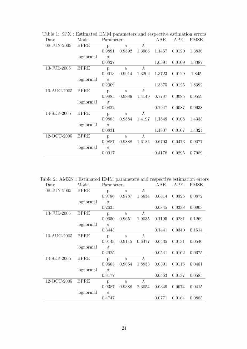
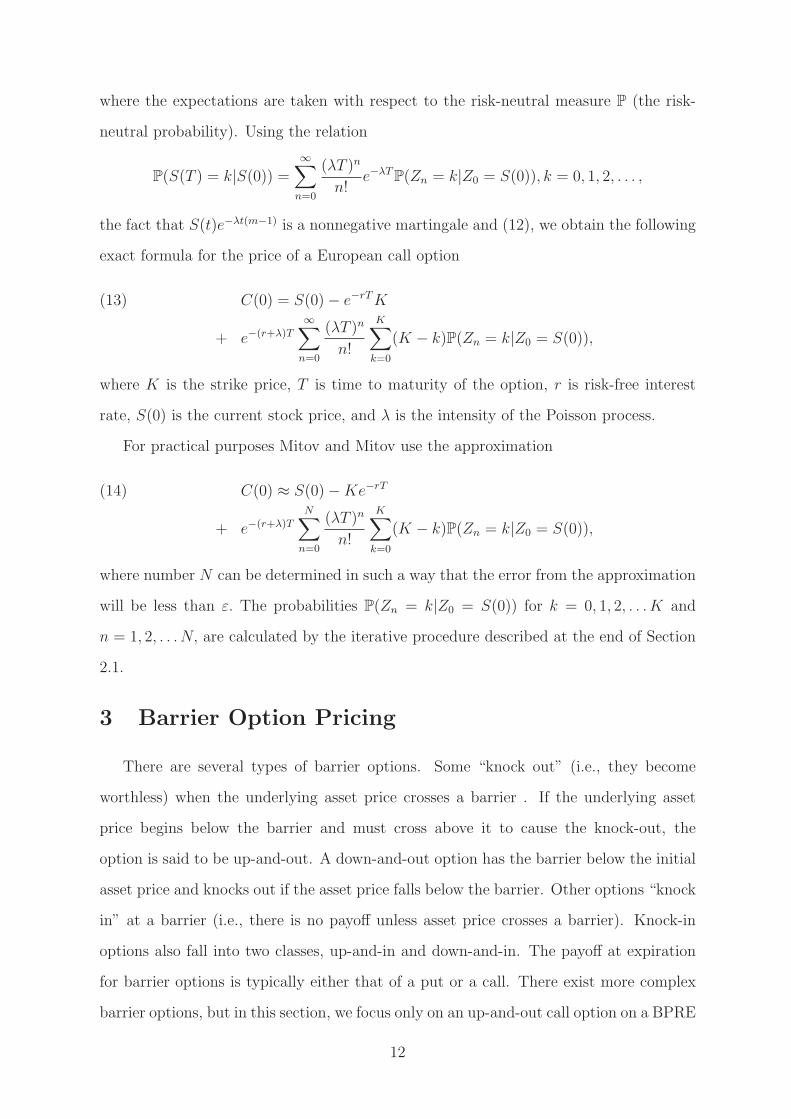
Table 1: SPX : Estimated EMM parameters and respective estimation errorsDate Model Parameters AAE APE RMSE
08-JUN-2005 BPRE p a λ
0.9891 0.9892 1.3968 1.1457 0.0120 1.3836lognormal σ
0.0827 1.0391 0.0109 1.3387
13-JUL-2005 BPRE p a λ
0.9913 0.9914 1.3202 1.3723 0.0129 1.845lognormal σ
0.2009 1.3375 0.0125 1.8392
10-AUG-2005 BPRE p a λ
0.9885 0.9886 1.4149 0.7787 0.0085 0.9559lognormal σ
0.0822 0.7947 0.0087 0.9638
14-SEP-2005 BPRE p a λ
0.9883 0.9884 1.4197 1.1849 0.0108 1.4335lognormal σ
0.0831 1.1807 0.0107 1.4324
12-OCT-2005 BPRE p a λ
0.9887 0.9888 1.6182 0.6793 0.0473 0.9077lognormal σ
0.0917 0.4178 0.0295 0.7989
Table 2: AMZN : Estimated EMM parameters and respective estimation errorsDate Model Parameters AAE APE RMSE
08-JUN-2005 BPRE p a λ
0.9786 0.9787 1.6634 0.0814 0.0325 0.0872lognormal σ
0.2635 0.0845 0.0338 0.0903
13-JUL-2005 BPRE p a λ
0.9650 0.9651 1.9035 0.1195 0.0281 0.1269lognormal σ
0.3445 0.1441 0.0340 0.1514
10-AUG-2005 BPRE p a λ
0.9143 0.9145 0.6477 0.0435 0.0131 0.0540lognormal σ
0.2925 0.0541 0.0162 0.0675
14-SEP-2005 BPRE p a λ
0.9663 0.9664 1.8833 0.0391 0.0115 0.0481lognormal σ
0.3177 0.0463 0.0137 0.0585
12-OCT-2005 BPRE p a λ
0.9387 0.9388 2.3054 0.0349 0.0074 0.0415lognormal σ
0.4747 0.0771 0.0164 0.0885
21

Table 3: INTC : Estimated EMM parameters and respective estimation errorsDate Model Parameters AAE APE RMSE
08-JUN-2005 BPRE p a λ
0.9850 0.9851 1.5135 0.0329 0.0273 0.0361lognormal σ
0.2456 0.0219 0.0153 0.0274
13-JUL-2005 BPRE p a λ
0.9860 0.9861 1.4860 0.0452 0.0320 0.0548lognormal σ
0.2308 0.0379 0.0269 0.0453
10-AUG-2005 BPRE p a λ
0.9891 0.9892 1.3954 0.0499 0.0364 0.0516lognormal σ
0.1895 0.0557 0.0407 0.0579
14-SEP-2005 BPRE p a λ
0.9859 0.9860 1.4893 0.0471 0.0425 0.0552lognormal σ
0.2535 0.0564 0.0512 0.0577
12-OCT-2005 BPRE p a λ
0.9813 0.9814 1.6031 0.0492 0.0344 0.0612lognormal σ
0.3091 0.0702 0.0493 0.0759
Table 4: MSFT : Estimated EMM parameters and respective estimation errorsDate Model Parameters AAE APE RMSE
08-JUN-2005 BPRE p a λ
0.9227 0.9235 0.1413 0.0670 0.0489 0.0791lognormal σ
0.1697 0.0748 0.0550 0.0862
13-JUL-2005 BPRE p a λ
0.9874 0.9875 1.2226 0.0350 0.0289 0.0355lognormal σ
0.2009 0.0446 0.0371 0.0463
10-AUG-2005 BPRE p a λ
0.9375 0.9382 0.1898 0.0384 0.1568 0.0424lognormal σ
0.1819 0.0591 0.0606 0.0730
14-SEP-2005 BPRE p a λ
0.9913 0.9915 1.3185 0.0212 0.0216 0.0213lognormal σ
0.1740 0.0143 0.0146 0.0144
12-OCT-2005 BPRE p a λ
0.9103 0.9110 0.1945 0.0265 0.0278 0.0316lognormal σ
0.2298 0.0409 0.0430 0.0506
22

Table 5: SPX : Up-and-Out and Standard Call Option Prices
Up-and-Out Call Option Prices
5 days to Maturity 38 days to Maturity 72 days to Maturity
Strike BPRE lognormal BPRE lognormal BPRE lognormal
1140 87.8365 88.0095 73.9546 70.2746 53.3410 49.03561160 67.8538 68.0250 56.9195 53.7793 40.3445 36.70791180 47.8757 48.0417 40.6091 38.0147 28.3509 25.40051200 28.0554 28.1845 25.9172 23.8965 17.9533 15.71391220 10.4329 10.6313 14.0213 12.5981 9.7494 8.22661240 1.6013 1.6579 5.8552 5.0065 4.1346 3.27651260 0.0979 0.0719 1.5141 1.1501 1.0921 0.75821270 0.0018 0.0005 0.0962 0.0444 0.0706 0.0295
Standard Call Option Prices
5 days to Maturity 38 days to Maturity 72 days to Maturity
Strike BPRE lognormal BPRE lognormal BPRE lognormal
1140 88.0133 88.0133 93.7358 93.7159 100.0277 99.96221160 68.0284 68.0283 74.1869 74.1452 81.2017 81.11141180 48.0482 48.0445 55.3628 55.3053 63.3820 63.28651200 28.2256 28.1868 38.1574 38.1121 47.1707 47.10261220 10.6010 10.6330 23.7500 23.7426 33.1932 33.18171240 1.7564 1.6591 13.0843 13.1021 21.9192 21.97051260 0.2344 0.0727 6.3007 6.2990 13.5034 13.59431270 0.1196 0.0007 2.6617 2.6066 7.7357 7.8258
The current value S(0) of the SPX is 1227.2 and the risk-free rate r is 0.0377 per annum.The barrier level is 1290 in order to be greater than all of the selected strike prices.
23

Table 6: AMZN : Up-and-Out and Standard Call Option Prices
Up-and-Out Call Option Prices
5 days to Maturity 38 days to Maturity 72 days to Maturity
Strike BPRE lognormal BPRE lognormal BPRE lognormal
39 4.0173 4.0962 2.3249 1.9097 1.3452 1.036840 3.0510 3.1285 1.8005 1.4481 1.0270 0.771841 2.1410 2.2189 1.3410 1.0517 0.7551 0.551142 1.3476 1.4268 0.9519 0.7240 0.5301 0.373843 0.7394 0.8116 0.6360 0.4656 0.3507 0.237344 0.3475 0.3989 0.3923 0.2735 0.2146 0.137945 0.1388 0.1649 0.2167 0.1412 0.1178 0.070646 0.0462 0.0548 0.1013 0.0597 0.0548 0.0297
Standard Call Option Prices
5 days to Maturity 38 days to Maturity 72 days to Maturity
Strike BPRE lognormal BPRE lognormal BPRE lognormal
39 4.1412 4.1369 4.8860 4.8689 5.6102 5.588240 3.1726 3.1652 4.1298 4.1182 4.9179 4.906941 2.2603 2.2515 3.4395 3.4348 4.2772 4.278942 1.4646 1.4553 2.8213 2.8239 3.6905 3.705343 0.8541 0.8361 2.2790 2.2879 3.1589 3.186544 0.4599 0.4193 1.8132 1.8264 2.6825 2.721745 0.2488 0.1813 1.4221 1.4367 2.2603 2.309146 0.1539 0.0671 1.1010 1.1136 1.8904 1.9462
The current price S(0) of the AMZN is 43.10 and the risk-free rate r is 0.0377 per annum.The barrier level is 49 in order to be greater than all of the selected strike prices.
24

Table 7: INTC : Up-and-Out and Standard Call Option Prices
Up-and-Out Call Option Prices
5 days to Maturity 38 days to Maturity 72 days to Maturity
Strike BPRE lognormal BPRE lognormal BPRE lognormal
23.00 1.4069 1.5200 1.7159 1.6759 1.6180 1.366123.50 0.9455 1.0580 1.3699 1.3459 1.3267 1.110224.00 0.5490 0.6570 1.0652 1.0548 1.0662 0.883624.50 0.2641 0.3530 0.8047 0.8046 0.8378 0.686725.00 0.1045 0.1598 0.5889 0.5953 0.6414 0.519025.50 0.0346 0.0599 0.4160 0.4254 0.4765 0.379726.00 0.0099 0.0184 0.2823 0.2918 0.3415 0.267026.50 0.0025 0.0046 0.1829 0.1905 0.2342 0.1786
Standard Call Option Prices
5 days to Maturity 38 days to Maturity 72 days to Maturity
Strike BPRE lognormal BPRE lognormal BPRE lognormal
23.00 1.5219 1.5200 1.9352 1.9557 2.2888 2.327423.50 1.0605 1.0580 1.5820 1.6058 1.9597 2.004124.00 0.6640 0.6570 1.2702 1.2948 1.6615 1.710224.50 0.3790 0.3530 1.0026 1.0247 1.3953 1.446325.00 0.2191 0.1598 0.7796 0.7956 1.1613 1.211925.50 0.1490 0.0599 0.5995 0.6059 0.9588 1.006426.00 0.1239 0.0184 0.4587 0.4525 0.7864 0.828326.50 0.1163 0.0046 0.3522 0.3315 0.6420 0.6756
The current price S(0) of the INTC is 24.49 and the risk-free rate r is 0.0377 per annum.The barrier level is 30 in order to be greater than all of the selected strike prices.
25

Table 8: MSFT : Up-and-Out and Standard Call Option Prices
Up-and-Out Call Option Prices
5 days to Maturity 38 days to Maturity 72 days to Maturity
Strike BPRE lognormal BPRE lognormal BPRE lognormal
25.00 1.2742 1.3326 1.5696 1.6149 1.7205 1.651825.50 0.8000 0.8576 1.1982 1.2469 1.3829 1.328026.00 0.3975 0.4534 0.8787 0.9292 1.0844 1.042526.50 0.1427 0.1819 0.6166 0.6661 0.8275 0.796827.00 0.0374 0.0518 0.4125 0.4579 0.6126 0.591027.50 0.0076 0.0100 0.2624 0.3010 0.4384 0.423528.00 0.0012 0.0013 0.1582 0.1883 0.3017 0.291528.50 0.0002 0.0001 0.0900 0.1115 0.1983 0.1909
Standard Call Option Prices
5 days to Maturity 38 days to Maturity 72 days to Maturity
Strike BPRE lognormal BPRE lognormal BPRE lognormal
25.00 1.3342 1.3326 1.6395 1.6452 1.9252 1.937425.50 0.8600 0.8576 1.2674 1.2752 1.5777 1.593526.00 0.4575 0.4534 0.9472 0.9552 1.2693 1.287826.50 0.2024 0.1819 0.6844 0.6900 1.0025 1.022027.00 0.0964 0.0518 0.4797 0.4797 0.7777 0.796027.50 0.0658 0.0100 0.3289 0.3205 0.5935 0.608428.00 0.0588 0.0013 0.2240 0.2057 0.4470 0.456228.50 0.0571 0.0001 0.1551 0.1268 0.3337 0.3357
The current price S(0) of the MSFT is 26.31 and the risk-free rate r is 0.0377 per annum.The barrier level is 32 in order to be greater than all of the selected strike prices.
26

0 0.05 0.1 0.15 0.2 0.25 0.3 0.3514
16
18
20
22
24
26
28
30
time to maturity (in years)
up−a
nd−o
ut c
all o
ptio
n pr
ice
BPRE and Lognormal Barrier Option Prices
LognormalBPRE
Figure 1: Up-and-out call option on SPX prices from BPRE model and lognormal modelas a function of time to maturity. The current value S(0) of the SPX is 1227.2, therisk-free rate r is 0.0377 per annum, the strike price is 1200, and the barrier level is 1290.
0 0.05 0.1 0.15 0.2 0.25 0.3 0.35
0.4
0.5
0.6
0.7
0.8
0.9
1
1.1
1.2
1.3
time to maturity (in years)
up−a
nd−o
ut c
all o
ptio
n pr
ice
BPRE and Lognormal Barrier Option Prices
LognormalBPRE
Figure 2: Up-and-out call option on AMZN prices from BPRE model and lognormalmodel as a function of time to maturity. The current price S(0) of the AMZN is 43.1,the risk-free rate r is 0.0377 per annum, the strike price is 42, and the barrier level is 49.
27
0 0.05 0.1 0.15 0.2 0.25 0.3 0.350.4
0.5
0.6
0.7
0.8
0.9
1
1.1
1.2
1.3
time to maturity (in years)
up−a
nd−o
ut c
all o
ptio
n pr
ice
BPRE and Lognormal Barrier Option Prices
LognormalBPRE
Figure 3: Up-and-out call option on INTC prices from BPRE model and lognormalmodel as a function of time to maturity. The current price S(0) of the INTC is 24.49,the risk-free rate r is 0.0377 per annum, the strike price is 24, and the barrier level is 30.
0 0.05 0.1 0.15 0.2 0.25 0.3 0.35
0.4
0.5
0.6
0.7
0.8
0.9
1
1.1
1.2
1.3
time to maturity (in years)
up−a
nd−o
ut c
all o
ptio
n pr
ice
BPRE and Lognormal Barrier Option Prices
LognormalBPRE
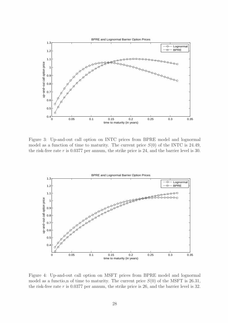
Figure 4: Up-and-out call option on MSFT prices from BPRE model and lognormalmodel as a functio,n of time to maturity. The current price S(0) of the MSFT is 26.31,the risk-free rate r is 0.0377 per annum, the strike price is 26, and the barrier level is 32.
28
Related Documents