BARREL-STAVE FLEXTENSIONAL TRANSDUCER DESIGN A THESIS SUBMITTED TO THE DEPARTMENT OF ELECTRICAL AND ELECTRONICS ENGINEERING AND THE INSTITUTE OF ENGINEERING AND SCIENCES OF BILKENT UNIVERSITY IN PARTIAL FULLFILMENT OF THE REQUIREMENTS FOR THE DEGREE OF MASTER OF SCIENCE By Aykut Şahin March 2009

Welcome message from author
This document is posted to help you gain knowledge. Please leave a comment to let me know what you think about it! Share it to your friends and learn new things together.
Transcript
BARREL-STAVE FLEXTENSIONAL
TRANSDUCER DESIGN
A THESIS
SUBMITTED TO THE DEPARTMENT OF ELECTRICAL AND
ELECTRONICS ENGINEERING
AND THE INSTITUTE OF ENGINEERING AND SCIENCES
OF BILKENT UNIVERSITY
IN PARTIAL FULLFILMENT OF THE REQUIREMENTS
FOR THE DEGREE OF
MASTER OF SCIENCE
By
Aykut Şahin
March 2009

ii
I certify that I have read this thesis and that in my opinion it is fully adequate, in
scope and in quality, as a thesis for the degree of Master of Science.
Prof. Dr. Hayrettin Köymen (Supervisor)
I certify that I have read this thesis and that in my opinion it is fully adequate, in
scope and in quality, as a thesis for the degree of Master of Science.
Prof. Dr. Yusuf Ziya İder
I certify that I have read this thesis and that in my opinion it is fully adequate, in
scope and in quality, as a thesis for the degree of Master of Science.
Assoc. Prof. Dr. Tolga Çiloğlu
Approved for the Institute of Engineering and Sciences:
Prof. Dr. Mehmet B. Baray
Director of Institute of Engineering and Sciences

iii
ABSTRACT
BARREL-STAVE FLEXTENSIONAL TRANSDUCER
DESIGN
Aykut Şahin
M.S. in Electrical and Electronics Engineering Supervisor: Prof. Dr. Hayrettin Köymen
March 2009
This thesis describes the design of low frequency, high power capability class-I
flextensional, otherwise known as the barrel-stave, flextensional transducer.
Piezoelectric ceramic rings are inserted inside the shell. Under an electric drive,
ceramic rings vibrate in the thickness mode in the longitudinal axis. The
longitudinal vibration of the rings is transmitted to the shell and converted into a
flexural motion. Low amplitude displacements on its axis create high total
displacement on the shell, acting as a mechanical transformer.
Equivalent circuit analysis of transducer is performed in MATLAB and the
effects of structural variables on the resonance frequency are investigated.
Critical analysis of the transducer is performed using finite element modeling
(FEM). Three dimensional transducer structure is modeled in ANSYS, and
underwater acoustical performance is investigated. Acoustical analysis is
performed by applying a voltage on piezoelectric material both in vacuum and in
water for the convex shape barrel-stave transducer. Effects of transducer
structural variables, such as transducer dimensions, shell thickness, shell
curvature and shell material, on the electrical input impedance, electro-
acoustical transfer function, resonance frequency and quality factor are
investigated. Thermal analysis of designed transducer is performed in finite
element analysis. Measured results of the transducer are compared with the
theoretical results.

iv
Keywords: Underwater Acoustic Transducer, Barrel-Stave, Flextensional
Transducer, Low Frequency, High Power, Piezoelectric.
v
ÖZET
1. SINIF GERİLİM İLE BÜKÜLEN AKUSTİK
DÖNÜŞTÜRÜCÜ TASARIMI
Aykut Şahin Elektrik ve Elektronik Mühendisliği Bölümü Yüksek Lisans
Tez Yöneticisi: Prof. Dr. Hayrettin Köymen Mart 2009
Bu tezde düşük frekanslarda yüksek güç gerektiren uygulamalara uygun 1. Sınıf
fıçı tipi, gerilim ile bükülen (Barrel-stave flextensional) akustik dönüştürücü
tasarımı tartışılmaktadır. Fıçı tipi dönüştürücünün iç kısmında halka tipi
piezoelektrik malzeme bulunmaktadır. Bu piezoelektrik malzemeye elektriksel
gerilim uygulanmakta ve piezoelektrik malzemede boylamsal hareket
oluşturulmaktadır. Fıçının orta kısmında oluşan boylamsal hareketler kabuk
kısmında bükülmelere neden olmaktadır. Bu şekilde fıçı mekanik bir
transformatör etkisi göstererek eksenindeki küçük genlikli titreşimleri geniş fıçı
yüzeyi marifeti ile ortama yükselterek aktarmaktadır.
Fıçı dönüştürücü eşdeğer devre çözümlemesi MATLAB programı ile
gerçekleştirilmiş ve fıçı parametrelerinin rezonans frekansı üzerindeki etkileri
incelenmiştir. Fıçının kritik analiz çözümlemeleri sonlu eleman modelleme
(Finite Element Model: FEM) yöntemi kullanılarak gerçekleştirilmiştir. ANSYS
programında, fıçı, su içerisinde üç boyutlu modellenerek akustik performansı
incelenmiştir. Akustik analizler piezoelektrik malzemeye gerilim uygulayarak,
boşlukta ve suda dışbükey fıçı tipi dönüştürücü için gerçekleştirilmiştir. Fıçı
boyutları, kabuk kalınlığı ve eğriliği, kabuk malzemesi gibi fıçının yapısal
parametrelerinin, dönüştürücünün elektriksel giriş empedansı, elektro-akustik
transfer fonksiyonu, rezonans frekansı, kalite faktörü üzerindeki etkileri
incelenmiştir. Tasarlanan dönüştürücü ısıl analizleri sonlu eleman modellemesi

vi
ile gerçekleştirilmiştir. Dönüştürücü ölçüm sonuçları teorik sonuçlar ile
karşılaştırılmıştır.
Anahtar Kelimeler: Sualtı Akustik Dönüştürücü, Barrel-Stave, Flextensional
Transducer, Düşük Frekans, Yüksek Güç, Piezoelektrik

vii
To my parents and my fiance…

viii
Acknowledgements
I would like to express my gratitude to my supervisor Prof. Dr. Hayrettin
Köymen for his instructive comments and guidance in the supervision of the
thesis. I would also like to express my special thanks to the jury members Prof.
Dr. Y. Ziya İder and Assoc. Prof. Dr. Tolga Çiloğlu for evaluating my thesis.
I would like to thank Zekeriyya Şahin, Sacit Yılmaz, and H. Kağan Oğuz for
providing valuable discussions and their support. I would like to thank A. Gözde
Ulu and other employees of ASELSAN who worked on the construction of
barrel-stave transducer.
I would like to express my gratitude to Prof. Dr. Aydın Doğan for his valuable
support in the production of alumina rings. I would also like to thank to Dr.
D.T.I. Francis for his kind and valuable help for overcoming the problem in the
modeling of transducer in ANSYS.
I would also like to express my thanks to my parents Bilal-Münevver Şahin, my
fiancé Özlem, and my sister and her family Aysun-Kemal-Ela Özkan for their
support and endless love throughout my life.
Finally, special thanks to the TUBITAK for its’ valuable financial support.

ix
Table of Contents
1. ACKNOWLEDGEMENTS............................................................... VII
2. LIST OF FIGURES..............................................................................XI
3. LIST OF TABLES............................................................................. XIV
4. INTRODUCTION .................................................................................. 1
1.1 HISTORY OF UNDERWATER ACOUSTICS ................................................ 3 1.2 UNDERWATER ACOUSTIC APPLICATIONS .............................................. 4 1.3 PIEZOELECTRIC EFFECT......................................................................... 5 1.4 FINITE ELEMENT METHOD (FEM)......................................................... 8 1.5 ELECTRICAL ANALOGS OF ACOUSTICAL QUANTITIES ......................... 10 1.6 BASIC TRANSDUCER PARAMETERS...................................................... 11
5. BARREL-STAVE TRANSDUCERS.................................................. 13
2.1 FLEXTENSIONAL TRANSDUCER CLASSIFICATION SCHEMES................. 13 2.2 APPLICATION AREAS OF BARREL-STAVE TRANSDUCERS .................... 15 2.3 BARREL-STAVE TRANSDUCERS ........................................................... 16
6. EQUIVALENT CIRCUIT REPRESENTATION............................. 18
3.1 BASIC TRANSDUCER EQUIVALENT CIRCUIT THEORY .......................... 18 3.2 AN EQUIVALENT CIRCUIT MODEL FOR BARREL-STAVE FLEXTENSIONAL
TRANSDUCER .................................................................................................. 21
7. DESIGN OF BARREL-STAVE TRANSDUCER USING
BRIGHAM’S EQUIVALENT CIRCUIT MODEL .......................... 26
4.1 SAMPLE EQUIVALENT CIRCUIT ANALYSIS .......................................... 26 4.2 COMPARISON OF EQUIVALENT CIRCUIT RESULTS AND FEM RESULTS 29
8. FINITE ELEMENT MODEL (FEM) MODEL OF BARREL-
STAVE FLEXTENSIONAL TRANSDUCER................................... 32
5.1 FINITE ELEMENT MODELING OF BARREL-STAVE FLEXTENSIONAL
TRANSDUCER IN ANSYS ................................................................................ 33 5.2 BARREL-STAVE FLEXTENSIONAL TRANSDUCER DESIGN IN ANSYS... 42 5.3 CORRECTION ON THE EQUIVALENT CIRCUIT USING FEM RESULTS .... 51
9. POWER LIMITATIONS OF BARREL-STAVE
FLEXTENSIONAL TRANSDUCER ................................................. 58
x
6.1 CAVITATION LIMITATION FOR BARREL-STAVE FLEXTENSIONAL
TRANSDUCER .................................................................................................. 59 6.2 THERMAL ANALYSIS OF BARREL-STAVE FLEXTENSIONAL TRANSDUCER
............................................................................................................ 62
10. EXPERIMENTAL WORK ................................................................. 70
7.1 CONSTRUCTION DETAILS OF BARREL-STAVE FLEXTENSIONAL
TRANSDUCER .................................................................................................. 70 7.2 MEASURED RESULTS OF BARREL-STAVE FLEXTENSIONAL TRANSDUCER
............................................................................................................ 75
11. CONCLUSION..................................................................................... 83
12. APPENDIX I......................................................................................... 85
THE ‘BASE’ VALUES OF THE STRUCTURE’S DIMENSIONS AND THE MATERIAL
PROPERTIES ..................................................................................................... 85
13. APPENDIX II ....................................................................................... 87
EFFECTIVE VIBRATING MASS OF STACK ......................................................... 87
14. APPENDIX III...................................................................................... 89
ELEMENT TYPES USED IN THE ANSYS MODEL .............................................. 89 MATERIAL MATRICES FOR PZT-4 ................................................................... 89
15. APPENDIX IV...................................................................................... 91
THERMAL PROPERTIES OF MATERIALS ............................................................ 91
16. APPENDIX V ....................................................................................... 92
CONSTRUCTION DETAILS OF BARREL-STAVE TRANSDUCER ........................... 92
17. APPENDIX VI .................................................................................... 102
MEASURED RESULTS FOR TRANSDUCER CONSTRUCTED WITH PETROLATUM 102
xi
List of Figures
Figure 1 The Pagliarini-White classification scheme......................................... 14 Figure 2 The Brigham-Royster classification scheme ....................................... 15 Figure 3 4-terminal representation of transducer ............................................... 18 Figure 4 Piezoelectric transducer’s general equivalent circuit........................... 21 Figure 5 Equivalent circuit model of barrel-stave flextensional transducer....... 21 Figure 6 (a) Fundamental, flexural mode; (b) Higher frequency extensional,
extensional mode. Dashed curve is undeformed stave shape..................... 25 Figure 7 Slotted-Shell Transducer...................................................................... 27 Figure 8 Staved-Shell Transducer ...................................................................... 27 Figure 9 In-water conductance-susceptance seen from the electrical terminals
obtained from equivalent circuit analysis................................................... 29 Figure 10 Convex Shell Class-I Flextensional Transducer ................................ 34 Figure 11 Inside view of the transducer model in ANSYS................................ 36 Figure 12 Top view of the transducer model in ANSYS ................................... 36 Figure 13 In-water transducer model in ANSYS ............................................... 37 Figure 14 Structure present (red) and structure absent (blue) fluid element types
in ANSYS model........................................................................................ 37 Figure 15 Conductance seen from the input terminals of transducer obtained
from FEM ................................................................................................... 38 Figure 16 Susceptance seen from the input terminals of transducer obtained
from FEM ................................................................................................... 39 Figure 17 Removed water elements just above the gap between the shell
components................................................................................................. 40 Figure 18 Conductance seen from the input terminals of transducer obtained
from FEM ................................................................................................... 40 Figure 19 Susceptance seen from the input terminals of transducer obtained
from FEM ................................................................................................... 41 Figure 20 PZT4 rings used in FEM analysis ...................................................... 42 Figure 21 Conductance seen from the input terminals of transducer for
aluminum shell and D3 design configuration............................................. 46 Figure 22 Susceptance seen from the input terminals of transducer for aluminum
shell and D3 design configuration.............................................................. 46 Figure 23 Conductance seen from the input terminals of transducer for
carbon/fiber epoxy shell and D3 design configuration .............................. 47 Figure 24 Susceptance seen from the input terminals of transducer for
carbon/fiber epoxy shell and D3 design configuration .............................. 47 Figure 25 Vacuum Conductance seen from the input terminals of transducer for
aluminum shell and D3 design configuration............................................. 48 Figure 26 Vacuum Susceptance seen from the input terminals of transducer for
aluminum shell and D3 design configuration............................................. 48 Figure 27 Source pressure level of barrel-stave transducer obtained from FEM
analysis ....................................................................................................... 49

xii
Figure 28 Normalized horizontal directivity pattern of barrel-stave transducer at resonance frequency ................................................................................... 50
Figure 29 Normalized vertical directivity pattern of barrel-stave transducer at resonance frequency ................................................................................... 50
Figure 30 Nodes located on stave that are used to calculate α and β ............. 53
Figure 31 Alfa vs Frequency obtained using the FEM results ........................... 53 Figure 32 Beta vs. Frequency obtained using the FEM results.......................... 54 Figure 33 Spherical radiation impedance used in barrel-stave equivalent circuit
.................................................................................................................... 55 Figure 34 Vacuum conductance-susceptance seen from the electrical terminals
obtained from equivalent circuit analysis................................................... 56 Figure 35 In-water conductance-susceptance seen from the electrical terminals
obtained from equivalent circuit analysis................................................... 56 Figure 36 Frequency dependence of cavitation threshold [2] ............................ 61 Figure 37 Maximum continuous wave acoustic power of barrel-stave transducer
at the onset of cavitation............................................................................. 62 Figure 38 FEM model of Barrel-Stave transducer in Flux2D............................ 63 Figure 39 Loss factor vs. rms electric field [18] ................................................ 64 Figure 40 Steady state temperature distribution of barrel-stave transducer in air
.................................................................................................................... 65 Figure 41 Transient temperature response of barrel-stave transducer taken from
the mid point of the model ......................................................................... 65 Figure 42 Steady state temperature distribution of barrel-stave transducer in
water ........................................................................................................... 66 Figure 43 Transient temperature response of barrel-stave transducer in water
taken from the mid point of the model ....................................................... 67 Figure 44 Steady state temperature distribution of barrel-stave transducer in
water with 3 mm polyurethane coating ...................................................... 68 Figure 45 Transient temperature response of barrel-stave transducer in water
with 3 mm polyurethane coating taken from the mid point of the model .. 68 Figure 46 Steady state temperature distribution of barrel-stave transducer in
water with 5 mm polyurethane coating ...................................................... 69 Figure 47 Transient temperature response of barrel-stave transducer in water
with 3 mm polyurethane coating taken from the mid point of the model .. 69 Figure 48 Cross-sectional view of barrel-stave transducer (scale 1:1)............... 71 Figure 49 Barrel-stave transducer without aluminum staves ............................. 72 Figure 50 Barrel-stave transducer with aluminum staves .................................. 74 Figure 51 Barrel-stave transducer sealed with silicon........................................ 75 Figure 52 Measured in-air input admittance of transducer without aluminum
staves .......................................................................................................... 76 Figure 53 Measured in-air input admittance of transducer with aluminum staves
.................................................................................................................... 77 Figure 54 Water tank with dimensions 2mX2m and 1.5m deep. ....................... 78 Figure 55 In-water conductance measured in water tank vs conductance obtained
in ANSYS................................................................................................... 78
xiii
Figure 56 In-water susceptance measured in water tank vs susceptance obtained in ANSYS................................................................................................... 79
Figure 57 Reservoir inside Bilkent University................................................... 80 Figure 58 In-water conductance measured in reservoir vs conductance obtained
in ANSYS................................................................................................... 80 Figure 59 In-water susceptance measured in reservoir vs susceptance obtained in
ANSYS....................................................................................................... 81 Figure 60 Basic static and end mass................................................................... 87 Figure 61 Element type selection window in ANSYS ....................................... 89 Figure 62 Measured in-air input admittance of transducer without aluminum
staves ........................................................................................................ 102 Figure 63 Measured in-air input admittance of transducer with aluminum staves
.................................................................................................................. 103

xiv
List of Tables Table 1 Analogy between the electrical and mechanical equations ................... 10 Table 2 Analogy between the electrical and mechanical parameters................. 10 Table 3 Comparison of Equivalent Circuit and FEM Results............................ 30 Table 4 Comparison of our ANSYS results and Bayliss’s FEM results ............ 41 Table 5 Structural design parameter values and in-water performance
characteristics of the staved shell transducer ............................................. 44 Table 6 Structural design parameter values and in-water performance
characteristics of the staved shell transducer for carbon/fiber epoxy shell element ....................................................................................................... 45
Table 7 Theoratical Results vs Measured Results.............................................. 82 Table 8 Structural parameters and their base values .......................................... 85 Table 9 Material Properties used in Clive Bayliss Thesis.................................. 85 Table 10 Carbon/Fiber Epoxy and Alumina Material Properties....................... 86 Table 11 Thermal properties of materials .......................................................... 91
1
Chapter 1
Introduction
Medium exhibits very different characteristics compared to air in terms
of propagation. Strong conductivity of salt water makes the water medium
dissipative for electromagnetic waves which means that their attenuation is
rapid, and their range is limited [1].
Acoustic waves are the only way today to carry information from one
point to another inside the water medium. Engineering science of sonar,
acronym of sound navigation and ranging, deals with the propagation of sound
in water. Sound propagation in active sonar systems is two-way that start from
the generation of sound by projector, which creates sound pressure waves
according to the applied electrical signals, and ending by the reception of echoes
by hydrophone, which converts incoming sound waves into electrical signals. In
passive sonar systems there is one-way propagation and the system listens the
sound radiated by the target using hydrophones [2].
There is a significant difference between the power handling limits of
projectors and hydrophones. Projectors are used as high power acoustic sources,
so their power handling levels are high, whereas power-handling levels of
hydrophones are low [3]. Therefore, due to the high power handling
requirements, projectors have more challenging design needs, and in this thesis
the design of barrel-stave flextensional projector is handled.
In the first chapter, we first give some historical background basically on
acoustics, and then we briefly discuss the application areas of acoustics in

2
military and civilian applications. Next, we discuss the piezoelectric effect,
piezoelectric materials and their properties. Afterwards, we explain the Finite
Element Modeling (FEM), which is used very often in transducer design. Then,
we describe the analogy between electromagnetic and acoustic waves. Finally,
we define the parameters used to define the transducer acoustical properties.
In the second chapter, we discuss the classification schemes and
application areas of barrel-stave transducer. Then, we summarize the related
works on barrel-stave transducers.
Third chapter deals with the equivalent circuit representation of barrel-
stave transducer. Firstly, we mention the basic equivalent circuit theory, and
then we describe the equivalent circuit model for the barrel-stave flextensional
transducer.
In the fourth chapter, we analyze the performance of barrel-stave
transducer equivalent circuit using the known structural parameter set and its
FEM results. Then, we compare the equivalent circuit and FEM results.
We will focus on the modeling and analysis of barrel-stave flextensional
transducer in ANSYS in the fifth chapter. First, we explain the modeling of
barrel-stave transducer in ANSYS. Then, we discuss the design of barrel-stave
transducer using FEM in ANSYS. Lastly, we make some correction on some
elements of the transducer equivalent circuit model of transducer using FEM
results.
In the sixth chapter, we analyze the power limitations of barrel-stave
flextensional transducer in terms of electrical limitations, cavitation limitations,
and thermal limitations.

3
In the seventh chapter, we describe the construction and measurement of
the designed transducer. First, we explain the steps and details of construction
process. Then, we measure the constructed transducer both in vacuum and
water.
1.1 History of Underwater Acoustics
One of the earliest references of the existence of sound at sea is from the
notebooks of the Leonardo da Vinci at the last quarter of 15th century. The first
quantitative measurement in underwater and sound occurred by the Swiss
physicist, Daniel Colladon, and French mathematician, Charles Sturm, in 1827
where they measure the velocity of sound [2].
In the 1840s, James Joule discovered the effect of magnetostriction [2].
In 1880, Jacques and Pierre Curie discovered piezoelectricity in quartz and other
crystals. The discoveries of these magnetostriction and piezoelectricity, which
are still used in most underwater transducers, have tremendous significance for
underwater sound [4].
In 1912, R.A. Fessenden developed a new type of moving coil
transducer, which was successfully used for signaling between submarines and
for echo ranging by 1914 [4].
At the beginning of World War II, active sonar system technology was
improved enough to be used by the Allied navies [1].
After the World War II, active sonars have grown larger and more
powerful and operate at frequencies several octaves lower than in World War II.
Therefore, the active sonar ranges improves to greater distances. In order to
increase the effective range of the passive sonar systems, their operational
4
frequencies decreased, which allows taking the advantage of the low frequency
ship noise of the submarines. However, at the same time the submarines have
become quiter, and have become far more difficult targets for passive detection
than before [2].
1.2 Underwater Acoustic Applications
Underwater acoustic technology is used in scientific, military and
industrial areas.
Most military underwater acoustic applications aimed at detecting,
locating, and identifying of targets. Depending on their functionality, military
sonars are classified into two categories [1];
Active sonars, which transmits and receives echoes returning from the
target.
Passive sonars which intercepts noises and active sonar signals radiated
by target.
Civilian applications are developed to meet the needs of scientific
programmes of environment study and monitoring, as well as the offshore
engineering and fishing. The main categories of civilian applications are as
follows [1];
Bathymetric sounders that measure the water depth.
Fishery sounders designed for the detection and localization of fish
shoals.
Sidescan sonars used for the acoustic imaging of the seabed.
Multibeam sounders used for seafloor mapping.
Sediment profilers used for the study of internal structure of the seabed.
Acoustic communication systems used as a telephone link and for the
transmission of digital data.

5
Positioning systems used to find the position of platforms.
Acoustic Doppler system used to measure the speed of sonar relative to
fixed medium, or the speed of water relative to a fixed instrument using the
frequency shift.
Acoustic tomography systems used to assess the structure of hydrological
perturbations.
1.3 Piezoelectric Effect
Jacques and Pierre Curie discovered piezoelectric effect in 1880. The
name is made up of two parts; piezo, which is derived from the Greek word for
pressure, and electric from electricity [5]. Literally, it means pressure - electric.
In a piezoelectric material, generation of electrical charge by the
application of mechanical force is called the direct piezoelectric effect.
Conversely, creating a change in mechanical dimensions by the application of
charge is called the inverse piezoelectric effect.
Several ceramic materials such as lead-zirconate-titanate (PZT), lead-
titanate (PbTiO2), lead-zirconate (PbZrO3), and barium-titanate (BaTiO3) have
been described as exhibiting a piezoelectric effect [5].
Ceramic material is made up of large numbers of randomly orientated
crystal grains. The ceramic material does not exhibit a piezoelectric effect in a
randomly oriented condition. Therefore, the ceramic must be polarized.
The ceramic materials are heated above a certain temperature called
Curie point and applied a high direct electric field. Under a strong and steady
electric field orientation of crystal grains partially aligned. Cooling the ceramic
below its curie point first and removing the electric field results in a remanent
6
polarization in ceramic material. In this polarized ceramic materials, in other
words piezoelectric materials there is a linear relation between the electrical
field and mechanical strain [4].
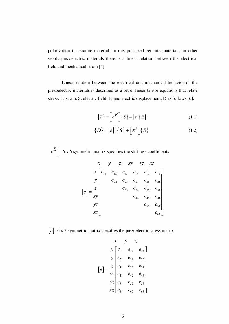
Linear relation between the electrical and mechanical behavior of the
piezoelectric materials is described as a set of linear tensor equations that relate
stress, T, strain, S, electric field, E, and electric displacement, D as follows [6]:
[ ] ET c S e E= −
(1.1)
[ ] T S
D e S Eε = + (1.2)
Ec
: 6 x 6 symmetric matrix specifies the stiffness coefficients
[ ]
11 12 13 14 15 16
22 23 24 25 26
33 34 35 36
44 45 46
55 56
66
x y z xy yz xz
c c c c c cx
c c c c cy
c c c czc
c c cxy
c cyz
cxz
=
[ ]e : 6 x 3 symmetric matrix specifies the piezoelectric stress matrix
[ ]
11 12 13
21 22 23
31 32 33
41 42 43
51 52 53
61 62 63
x y z
e e ex
e e ey
e e eze
e e exy
e e eyz
e e exz
=

7
Sε : 3 x 3 dielectric matrix
11
22
33
0 0
0 0
0 0
S
ε
ε ε
ε
=
General Comparison of Piezoelectric Ceramics
Ceramic-B is a modified barium titanate, which offers improved
temperature stability and lower aging in comparison with unmodified barium
titanate.
PZT-4 is recommended for high power acoustic radiating transducers
because of its high resistance to depolarization and low dielectric losses under
high electric drive. Its high resistance to depolarization under mechanical stress
makes it suitable for use in deep-submersion acoustic transducers and as the
active element in electrical power generating systems.
PZT-5A is recommended for hydrophones or instrument applications
because of its high resistivity at elevated temperatures, high sensitivity, and high
time stability.
PZT-8 is similar to PZT-4, but has even lower dielectric and mechanical
losses under high electric drive. It is recommended for applications requiring
higher power handling capability than is suitable for PZT-4.
Military specification for classifies ceramics into four basic types [7],
Type I (PZT-4)
Hard lead zirconate-titanate with a Curie temperature equal to or greater
than 310ºC

8
Type II (PZT-5A)
Soft lead zirconate-titanate with a Curie temperature equal to or greater
than 330ºC
Type III (PZT-8)
Very hard lead zirconate-titanate with a Curie temperature equal to or
greater than 330ºC
Type IV (Ceramic-B)
Barium titanate with nominal additives of 5 percent calcium titanate and
0.5 percent cobalt carbonate as necessary to obtain a Curie temperature equal to
or greater than 100ºC
The terms ‘hard’ and ‘soft’ refer to the composition type. Hard materials
are not easily poled or de-poled except at elevated temperatures which make
these materials suitable for projector that operate at high power levels. Soft
materials are more easily poled or de-poled. They have high electro-mechanical
coupling coefficients, which makes these materials suitable for hydrophones, or
low power projectors.
1.4 Finite Element Method (FEM)
Finite element method first appeared in 1960, when it was used in a
paper on plane elasticity problems. In the years since 1960 the finite element
method has received widespread acceptance in engineering [8].
Many problems can be solved approximately using a numerical analysis
technique called the finite element method.
In the finite element method the problem is reduced to a finite element
unknown problem by dividing the structure into a finite number of smaller sub

9
regions or finite elements. The ‘coarseness’ of these elements determines the
accuracy of the solution. Therefore, as the number of elements increases
approximation to the actual solution improves [7].
Applying an approximation function (interpolation function) within each
element, the actual infinite number of unknown problem can be well
transformed into a finite element problem [7, 8]. Each field variable is defined at
specific points on structure called nodes. The nodal values of the field variable
and the interpolation functions for the elements completely define the behavior
of the field variable within the elements [8].
In practice, a finite element analysis usually consists of three principal
steps [9]:
Preprocessing: Model construction part
Analysis: Constructed model is solved
Postprocessing: Examining the solution
For harmonic vibration at a frequency w, in radians per second the finite
element equation becomes [7, 10]:
[ ] [ ] 2nw M K u F − + = (1.3)
where [M] is the mass matrix, [K] is the stiffness matrix, and F is the
electromechanical forcing function.
The solution set is obtained by solving the above equation on each node.
10
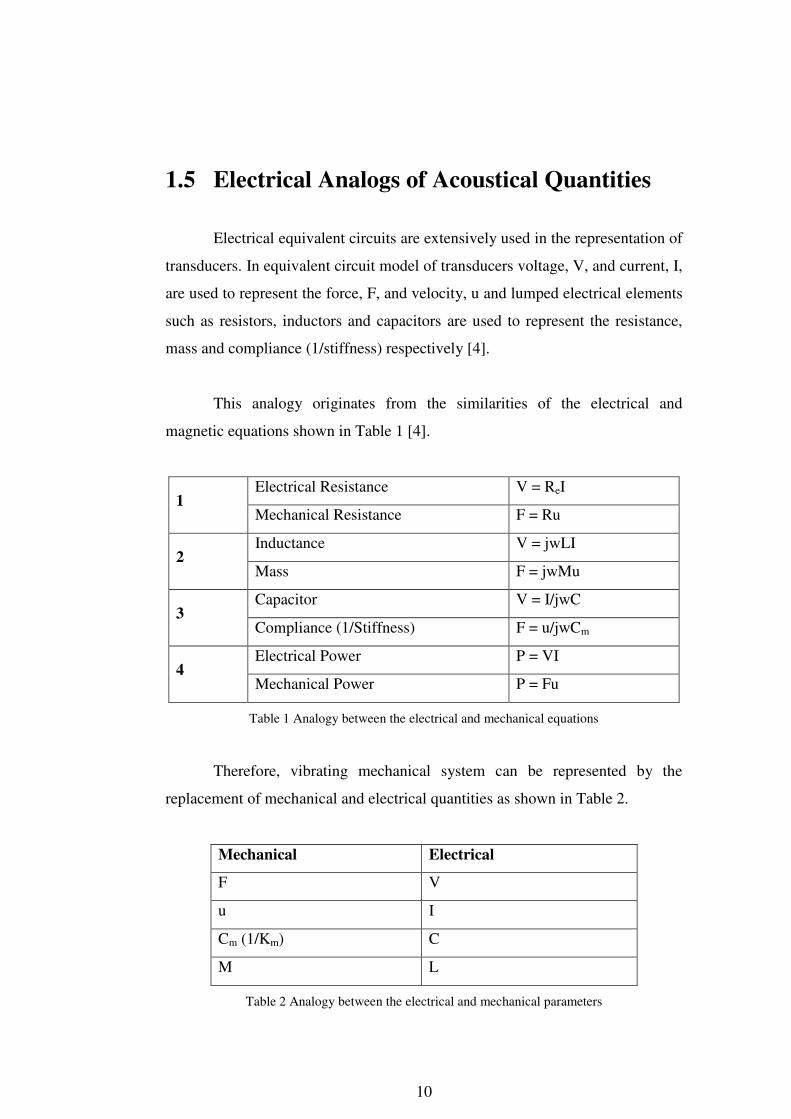
1.5 Electrical Analogs of Acoustical Quantities
Electrical equivalent circuits are extensively used in the representation of
transducers. In equivalent circuit model of transducers voltage, V, and current, I,
are used to represent the force, F, and velocity, u and lumped electrical elements
such as resistors, inductors and capacitors are used to represent the resistance,
mass and compliance (1/stiffness) respectively [4].
This analogy originates from the similarities of the electrical and
magnetic equations shown in Table 1 [4].
Electrical Resistance V = ReI 1
Mechanical Resistance F = Ru
Inductance V = jwLI 2
Mass F = jwMu
Capacitor V = I/jwC 3
Compliance (1/Stiffness) F = u/jwCm
Electrical Power P = VI 4
Mechanical Power P = Fu
Table 1 Analogy between the electrical and mechanical equations
Therefore, vibrating mechanical system can be represented by the
replacement of mechanical and electrical quantities as shown in Table 2.
Mechanical Electrical
F V
u I
Cm (1/Km) C
M L
Table 2 Analogy between the electrical and mechanical parameters

11
1.6 Basic Transducer Parameters
Some definitions and formulas related to the transducers and
hydrophones are listed below;
1. Directivity Index [2]:
1010log DT
Nond
IDI
I
=
(1.4)
where T emphasizes that the transmitting directivity index
ID: Directional pattern intensity
INond: Nondirectional pattern intensity
2. Source Level or Source Pressure Level [3, 11]:
Sound pressure (acoustic power) in dB referenced to 1.0 µPa measured at
1meter from the sound source.
( )1010logint 1
Intensityof sourceSL
reference ensity Paµ
=
(1.5)
( )( )10( 1 ) 170.9 10logr T
SL dB re Pa radiated power P DIµ = + + (1.6)
Source level can also be defined as pressure level referenced to 1.0 µPa
in dB scale as;
10( 1 ) 20log rms
ref
pSL dB re Pa
pµ
=
(1.7)

12
3. Transmitting Voltage Response [11]:
Transmitting Voltage Response (TVR) is the pressure level at 1m range
per 1 V of input voltage as a function of frequency.
4. Sensitivity [2]:
Hydrophone sensitivity is given in dB referenced to 1 Volt/µPa (dB re 1
V/µPa)
5. Beam Width [2]:
The width of the main beam lobe, in degrees, of the transducer. It is
usually defined as the width between the "half power point" or "-3dB" point.
6. Efficiency [2]:
In a projector, efficiency is defined as the ratio of the acoustic power
generated to the total electrical power input. Efficiency varies with frequency
and is expressed as a percentage.
7. Quality Factor [2]:
0
2 1
fQ
f f=
− (1.8)
where f0 : Resonance Frequency
(f2-f1) : Bandwidth

13
Chapter 2
Barrel-Stave Transducers
Throughout this chapter, the classification schemes of flextensional
transducers and the application areas of barrel-stave flextensional transducers
are discussed. In addition, we have summarized the previous works on barrel-
stave transducers.
We have divided this chapter into three sections. Two different
classification schemes of flextensional transducers that are the Pagliarini-White
scheme and the Brigham-Royster scheme are clarified in section 2.1. In section
2.2 the application areas of barrel-stave transducers and the advantages of
barrel-stave transducers compared to others in low frequency and high power
applications are mentioned. In section 2.3, the previous works on the design of
barrel-stave transducer are analyzed.
2.1 Flextensional Transducer Classification
Schemes
There are two classification schemes for the flextensional transducers,
one is the Pagliarini-White classification scheme and the other is the Brigham-
Royster classification scheme.
The criteria that is used to distinguish the four classes defined in
Pagliarini-White scheme, as shown in Figure 1, is based on shape [7, 12].

14
Figure 1 The Pagliarini-White classification scheme
In Brigham-Royster scheme, as shown in Figure 2, more complex
method is used. Classes I, IV, V are distinguished by shell shape. However,
classes I, II, and III are distinguished by pragmatic criteria; class II is a high
power version of class I and class III is a broadband version of class I [7, 12]. In
this classification scheme, the class-I flextensional type transducer is also known
as the barrel-stave flextensional transducer.

15
Figure 2 The Brigham-Royster classification scheme
2.2 Application Areas of Barrel-Stave
Transducers
In sonar and oceanography applications, the design of low frequency,
high power, underwater acoustic projectors have a high propriety.
New technology ship designs reduce the own ship noise of submarines,
so the usefulness of the passive towed arrays has been substantially diminished.
Thus long-range detection in underwater applications can now only be made by
using low-frequency active sonar systems [13].
16
In oceanography applications, low frequency projectors have been used
to track the deep oceanic water circulations, calculate the sound speed in water,
and communicate with the offshore systems [13].
Barrel-stave transducers are used in vertical array arrangements to
improve the horizontal directivity, and reduce the unwanted acoustic energy
transmission to the ocean floor and to the sea surface [14].
2.3 Barrel-Stave Transducers
The barrel-stave transducer consists of a piezoelectric stack and a
surrounding mechanical shell that is cylindrical. The mechanical shell has slots
along the axial z-direction in order to reduce the axial stiffness and decrease the
resonance frequency of the transducer. Under an electric drive, the ceramic stack
vibrates in the thickness mode in the longitudinal axis, which results in the end
plates extend in the axial direction. The axial vibration of the end plates is
transmitted to the shell and converted into a flexural motion.
The equivalent circuit of the barrel-stave transducer, which is described
by the modified Brigham’s equivalent circuit model, demonstrates the
mechanical characteristics of transducer in electrical circuit form [15]. Detailed
description of the equivalent circuit is given in chapter 3.
Although it provides reliable results, many assumptions have made
during the equivalent circuit analysis. Finite Element Analysis has made to see
the effects of the ignored parameters on the performance of the transducer.
D.T.I. Francis has investigated the effects of the structural parameters on
the performance of the transducer in FEA [14].
17
In Clive Bayliss’s doctorate thesis, he has also investigated the effects of
the structural parameters on the performance of the transducer in FEA. He has
compared the measured results with the theoretical results obtained by FEA and
found that they are consistent [7].
Soon Suck Jarng compares the barrel-stave sonar transducer simulation
between a coupled FE-BEM and ATILA, which has a BEM (Boundary Element
Method) solver and found that FE-BEM results agree well with the ATILA
results.
In the following chapters, the design of barrel-stave transducer using
both the equivalent circuit and FEA is explained. We use MATLAB for the
equivalent circuit analysis and ANSYS for the FEA.
18
Chapter 3
Equivalent Circuit Representation
Using the analogy between the electrical and mechanical systems,
mechanical systems such as transducers can be represented by an electrical
equivalent circuit. Electrical equivalent circuit analysis provides powerful
insight on the effects of each design parameters to the performance of
transducer.
Using this analogy, theory of the basic transducer equivalent circuit
modeling is mentioned in section 3.1. Derivation of equivalent circuit of
transducer describes methods of how the mechanical parameters of transducer
are represented by their electrical analogs. Section 3.2 describes the modified
Brigham’s equivalent circuit for the barrel-stave flextensional transducer.
3.1 Basic Transducer Equivalent Circuit Theory
Piezoelectric transducers can be represented by a 4-terminal network as
illustrated in Figure 3.
1
2
3
4
ui
V F Zr
Figure 3 4-terminal representation of transducer

19
First and second terminals shown in Figure 3 represent the input
electrical terminals, whereas third and fourth terminals represent the output
mechanical terminals [3].
When an alternating voltage V is applied to the input terminals, by
piezoelectric behavior of the transducer, alternating force F is generated at the
output terminals. In this case the radiation impedance r
Z of transducer can be
formulated as follows;
r
FZ
u=
− (3.1)
As a consequence of the reciprocal nature of the transducer, when an
alternating force F is applied to the output terminals, alternating voltage V is
generated at the input terminals. Therefore, transducer behaves as a transformer
that converts between electrical and mechanical quantities with a transformation
ratio N [3].
When transducer is in the radiation state into r
Z , the input current of the
transducer in terms of the applied input voltage V is formulated as follows;
ei Y V Nu= − (3.2)
where e
Y is the blocked electrical input impedance. In piezoelectric transducers
eY is the parallel combination of the clamped capacitance 0C and the dielectric
loss resistance e
R .
If an alternating force F is applied to the mechanical terminals, the
relation between the force and the displacement u is formulated as follows;
20
m
F NV Z u= + (3.3)
where m
Z is the mechanical impedance at the mechanical terminals when
0V = .
Combination of the equations in (3.1), (3.2), and (3.3) gives an electrical
input current as;
2
e
m r
N Vi Y V
Z Z= +
+ (3.4)
So the input impedance in
Y is;
2
in e
m r
N VY Y
Z Z= +
+ (3.5)
The mechanical impedance m
Z of a transducer is the series combination
of the mechanical compliance m
C , which is the inverse of the effective stiffness
K , effective vibrating mass M , and the mechanical loss resistance m
R as
illustrated below [3];
1m m
m
Z R jwMjwC
= + + (3.6)
Using the above circuit element expressions, piezoelectric transducer’s
equivalent circuit model is obtained as shown in Figure 4.
21
Ye
Zm
Zr
1 : N
Figure 4
3.2 An Equivalent Circuit Model for Barrel-
Stave Flextensional Transducer
Equivalent circuit model of barrel-stave flextensional transducer is
shown in Figure 5 [15].
1 : 1 :1 : N
Cb Gb
CmE
Cg
Ctr Md Rd
Cp
Mp
Rp
Cs Ms Rs
Mr Rr
Figure 5 Equivalent circuit model of barrel-stave flextensional transducer
In piezoelectric driver side bC is the blocked capacitance of the
piezoelectric rings driven in 33 mode, bG is the electrical loss conductance of
piezoelectric rings, N is the electromechanical transformation ratio, EmC is the
short circuit compliance of the rings, gC is the adhesive joints between the
rings, trC is the center bolt compliance, dM is the driver mass, dR is the driver
loss factor.
In the mechanical side of staves, pC , pM , and pR represent the higher
frequency extensional mode compliance, mass, loss resistance, respectively, of

22
staves. α represents the transformation of axial motion on either side of staves
to the radial motion. s
C , s
M , and s
R represent the fundamental flexural mode
compliance, mass, loss resistance, respectively, of staves. β is the
transformation of rms displacement to average displacement on staves in the
radial direction where rms and average displacements are calculated as;
2
1
1 n
rms in
ξ ξ= ∑ (3.7)
1
1 n
average i
inξ ξ
=
= ∑ (3.8)
rM and
rR are the radiation mass and radiation resistance of transducer,
respectively.
The piezoelectric driver side equivalent circuit element formulations are;
233 /S
bC n A lε= (3.9)
tanb b e
G wC δ= (3.10)
33 33 /EN nd Y A l= (3.11)
33/E E
mC l Y A= (3.12)
( 1) /g g g
C n l Y A= + (3.13)
tan / ( )Ed d m gR w C Cδ= + (3.14)
/tr tr tr tr
C l Y A= (3.15)
/( )d h t h t
M M M M M= + (3.16)
where n is the number of rings in the piezoelectric stack, 33Sε is the blocked
permittivity, l is the stack length (along the transducer axis), A is the stack
cross sectional area, tane
δ is the electrical loss factor, w is the angular
23
frequency, 33d is the piezoelectric constant, 33E
Y is the short circuit Young’s
modulus of the piezoelectric material, g
l is the bond thickness, g
Y is the
adhesive modulus, tand
δ is the driver loss factor, tr
l is the center bolt length,
trY is the center bolt Young’s modulus,
trA is the center bolt cross-sectional
area.
In the driver mass, d
M , equation, h
M is the corrected head mass, and
tM is the corrected tail mass where they are the combinations of the ring-stack
and end masses expressed as follows:
/ 3h h
M m Alρ φ= + (3.17)
( 1) / 3t t
M m Alρ φ φ= + − (3.18)
where ρ is the piezoelectric density, h
m and t
m are the actual head and tail
masses, respectively, and φ is
( 2 / 3) /( / 3)h t t
m m Al m Alφ ρ ρ= + + + (3.19)
The stave mechanics side equivalent circuit element formulations are;
/p s s
C l vY bh= (3.20)
tan /p p p
R wCδ= (3.21)
2( 1) / 3p s sM v bhlρ φ φ= − (3.22)
0.83(1 0.14 / ) /s s
l r l rα ≅ + (3.23)
s s sM v bhlρ= (3.24)
30.024( / ) /s s s
C l h vY b= (3.25)
tan /s s s
R wCδ= (3.26)

24
1.2β = (3.27)
3/ 20 ( ) / 2
r sM dlπρ= (3.28)
0 0r sR dl cπ ρ= (3.29)
where s
l is the unsupported stave length, b is an average stave width, h is an
average stave thickness, v is the number of staves, s
Y is the stave material
Young’s modulus, s
ρ is the stave material density, and tanp
δ is a loss factor
for the higher mode, r is the radius of curvature, tans
δ is the stave loss factor,
0ρ is the water density, 0c is the sound speed in water medium, and d is the
mean diameter of the radiating surface ( /d vb π≅ ) .
Barrel-stave flextensional transducers have two modes of operation in
terms of the behavior of staves with the end masses. In equivalent circuit model,
the p
C , p
M , and p
R resonator represents the higher frequency extensional
mode, whereas the s
C , s
M , and s
R resonator (to which is added the radiation
load of the water medium) represents the fundamental, flexural mode of the
transducer. In fundamental, flexural mode of the transducer, all surfaces expand
and contract in phase that means the end mass motion is in phase with the radial
motion of the staves, whereas in higher frequency extensional mode of the
transducer, end mass displacement and the stave radial displacements are out of
phase.
The fundamental, flexural motion where the convex stave is displaced
radially inward as the ends are stretched is shown in Figure 6 (a), whereas, the
higher frequency, extensional motion where the convex stave bends, as the ends
are stretched is shown in Figure 6 (b).
25
Figure 6 (a) Fundamental, flexural mode; (b) Higher frequency extensional, extensional mode. Dashed curve is undeformed stave shape.

26
Chapter 4
Design of Barrel-Stave Transducer
Using Brigham’s Equivalent Circuit
Model
In chapter 3, the equivalent circuit representation of barrel-stave
flextensional transducer is given. Some parameters of this equivalent circuit
model is derived using the FEM results and includes some approximations.
Clive Bayliss founds that the mathematical analysis difficult and the
optimization using the large number of variables complicated. Therefore, he
carried out his work using the finite element and boundary element methods to
design the barrel-stave flextensional transducer [7].
In this chapter, we compare the Brigham’s modified equivalent circuit
model results with the Clive Bayliss’s results in order to determine the
consistency between the equivalent circuit model and FEM.
4.1 Sample Equivalent Circuit Analysis
In Clive Bayliss’s Thesis, there are some FEM results obtained from
different designs. He has carried out his barrel-stave flextensional transducer
design for both slotted-shell and staved-shell transducer types. In both types the

27
shell section consists of number of sections known as staves. In slotted-shell
configuration the shell is circular in the hoop direction; however, in staved-shell
configuration staves are curved in the axial direction but flat in the hoop
direction. Slotted-shell and staved-shell structures are illustrated in Figure 7 and
Figure 8, respectively.
Figure 7 Slotted-Shell Transducer (top view)
Figure 8 Staved-Shell Transducer (top view)
28
Staved-shell type has lower resonance frequency and lower acoustic
power compared to the slotted-shell configuration. Our aim is to obtain the
transducer with low resonance frequency, so we focus on the design of staved-
shell flextensional transducer design.
The structural dimensions and the material properties that are used by
Clive Bayliss are listed in Appendix I.
We used the material properties and the structural dimensions given in
appendix I in the barrel-stave equivalent circuit. Young’s modulus of PZT-4
rings, Y , depends on the sound speed inside the PZT-4 material, u , and density
of PZT-4 material, ρ ,as;
2Y u ρ= (4.1)
Assuming the sound speed as 4000 /u m s= , Young’s modulus of PZT-4
rings becomes 120.8Y GPa= .
Using the structural variables and Young’s modulus as mentioned above,
conductance and susceptance of transducer that is seen from the electrical
terminals of the equivalent circuit is given in Figure 9.
The power that is transmitted into the transducer is directly proportional
to the input conductance as;
2
1
2
VP R
Z= (4.2)

29
Conductance curve gives the information about the power characteristics
of the transducer as shown in Eq. 4.2. Therefore, conductance and susceptance
graphs have high importance for estimating the performance of the transducer.
0.5 1 1.5 2 2.5 30
0.5
1
1.5x 10
-4
Co
nd
ucta
nce
(S
)
0.5 1 1.5 2 2.5 30
0.5
1
1.5x 10
-4
Su
sce
pta
nce
(S
)
Frequency (kHz)
Figure 9 In-water conductance-susceptance seen from the electrical terminals obtained from equivalent circuit analysis
4.2 Comparison of Equivalent Circuit Results
and FEM Results
Clive Bayliss has calculated the in water performance of the transducer
using the same physical parameters and material orientations as in our
equivalent circuit analysis using the FEM method. Bayliss found the
fundamental resonance frequency of the transducer as 925 Hz and bandwidth as
215 Hz. However, our equivalent circuit results do not match with these results.
In equivalent circuit analysis we find that the fundamental resonance frequency

30
of the transducer is 1500 Hz and the bandwidth is 750 Hz. The comparison of
these results is shown in Table 3.
Equivalent Circuit
Results FEM Results
Fundamental
Resonance Frequency 1500 Hz 925 Hz
Bandwidth 750 Hz 215 Hz
Quality Factor 2 4.3
Table 3 Comparison of Equivalent Circuit and FEM Results
In equivalent circuit analysis we apply equal head and tail masses, which
makes 2φ = . In this situation the actual head and tail masses become;
/ 6h h
M m Alρ= + (4.3)
/ 6t t
M m Alρ= + (4.4)
In appendix II, the contribution of the ceramic stack to the actual head
and tail masses is illustrated. In barrel-stave transducer the nodal plane, where
the displacement in the axial direction is zero, is the center of the ceramic stack
and the contribution of the ceramic stack mass to head and tail masses is the
one-sixth of its static mass. Therefore, the corrected head and tail mass formulas
for the equal head and tail mass situation, which are given in Eq. 4.3 and Eq.
4.4 are correct.
In equivalent circuit analysis, we take the sound speed inside the PZT-4
material as 4000 m/s. The sound speed inside the PZT-4 material varies between
2930 m/s and 4600 m/s. Therefore; the error in the selection of the sound speed
may cause the mismatch between the equivalent circuit and the FEM results.

31
In the model, the transformation of axial motion on either side of staves
to the radial motion is represented by α . For curved staved of rectangular cross
section with various values of s
l , unsupported stave length, h , average stave
thickness, and r , radius of curvature, α was value calculated using the finite
element computations and for / 0.1s
h l ≤ and 0.2 / 1s
l r≤ ≤ , the approximate
formula for α is found as in Eq. 3.23. In addition, the transformation ratio β is
also calculated using the finite element results as in Eq. 3.27.
The reason of the mismatch between the equivalent circuit result and
FEM results might be the errors in α and β transformation ratios.
We find out some problems stated above in the equivalent circuit model
for barrel-stave flextensional transducers. Equivalent circuit of barrel-stave
transducer is complicated and has some problems. Therefore, we have
proceeded the design phase with FEM analysis. The equivalent circuit model is
improved by modifying some of the equivalent circuit elements as discussed in
Section 5.3.

32
Chapter 5
Finite Element Model (FEM) Model
of Barrel-Stave Flextensional
Transducer
Transducer design consists of two major steps; equivalent circuit
analysis and finite element analysis. Equivalent circuit model contains the
lumped element representations of transducer’s fundamental elements that have
the significant influence on its performance. For some transducer types which
has relatively less complicated structure, equivalent circuit results well
approximates to the actual results, whereas for transducers that have
complicated structure, as in the case of barrel-stave flextensional transducer,
representing all significant components in equivalent circuit model may be
difficult, so the equivalent circuit results may be erroneous and less reliable.
In finite element analysis, depending on the symmetry of the structure,
modeling is carried out in 2D or 3D. Complete structure of the transducer is
divided into smaller sub pieces called elements. Reducing the element size,
which increases the number of elements used in model proportionally, can
increase accuracy in the modeling of transducer. Therefore, with the accurate
material properties used in the model and smaller element size, it is possible to
design transducers whose predicted results agree well with the measured results
[4].
33
Finite element analysis (FEA) may be initiated with the FEM transducer
models without water loading to simulate the operation of the transducer in air.
Afterwards, the FEM fluid field is added to the model, which has absorbers at an
appropriate distance from the transducer. The reflected pressure waves in water
structure causes the degradation in the performance of the transducer. Therefore,
at the outer side of the fluid ‘ρc’ matched absorber elements or special elements
that apply infinite acoustic continuation are used. The fluid field must be large
enough to apply the proper radiation mass loading to transducer [4].
Fluid elements that constitute the finite element acoustic medium
describe the pressure field with pressure values at the nodes of the elements;
however, mechanical elements are described with displacement values at the
nodes [4].
This chapter focuses on the design of barrel-stave transducer using FEM.
In section 5.1 the modeling process of transducer in 3D and the verification of
the model with the Bayliss’s results are described. Design of barrel-stave
transducer for various structural dimensions and materials are described in
section 5.2. Lastly, in section 5.3 we make corrections on the equivalent circuit
using the FEM results.
5.1 Finite Element Modeling of Barrel-Stave
Flextensional Transducer in ANSYS
2-dimensional longitudinal section of convex shell type barrel-stave
flextensional transducer is illustrated in Figure 10. Transducer’s mid-plane
inside the shell, the ring type PZT ceramic materials that operate in thickness
mode are placed in reverse polarized order. The dark and the light blue sections
in the 2D model represent the polarization directions of PZT elements. Shell

34
elements are located in the left and right side of the model as red and the head
sections which also represented by red are located bottom and top of the model.
The electrical insulator section between the PZT ceramics and the head elements
are illustrated by purple. All of these transducer elements kept together using
the center bolt that is located in the transducer mid-plane.
Figure 10 Convex Shell Class-I Flextensional Transducer
2D FEM model cannot be used due to slotted-shell configuration.
However, using the symmetry along the half plane of the transducer only the
half of the transducer is modeled in 3D. The transducer 3D transducer model in
vacuum and in water is illustrated in Figure 11, Figure 12 and Figure 13.
Element types used in the transducer model are given in Appendix III.
SOLID5 three-dimensional solid elements are used for PZT, steel, aluminum,
macor and araldite elements. For PZT elements UX, UY, UZ and VOLT degree
of freedoms (DOF) are chosen, and for other SOLID5 elements UX, UY, UZ
DOFs are chosen. SOLID5 has a 3-D magnetic, thermal, electric, piezoelectric
35
and structural field capability with limited coupling between the fields. The
element has eight nodes with up to six degrees of freedom at each node. When
used in structural and piezoelectric analyses, SOLID5 has large deflection and
stress stiffening capabilities [16]. FLUID30 three-dimensional fluid elements are
used to model the acoustical medium. FLUID30 elements that have a contact
with solid elements are arranged as the structure present, other fluid elements
are set as the structure absent elements. In Figure 14, red elements represent the
structure present FLUID30 elements and blue elements represent the structure
absent FLUID30 elements. FLUID30 is used for modeling the fluid medium and
the interface in fluid/structure interaction problems. Typical applications include
sound wave propagation and submerged structure dynamics. The governing
equation for acoustics, namely the 3-D wave equation, has been discretized
taking into account the coupling of acoustic pressure and structural motion at the
interface [16]. In order to prevent the reflection in the model, the FLUID130
infinite acoustic elements are used at the outer side of the model. FLUID130
simulates the absorbing effects of a fluid domain that extends to infinity beyond
the boundary of the finite element domain that is made of FLUID30 elements.
FLUID130 realizes a second-order absorbing boundary condition so that an
outgoing pressure wave reaching the boundary of the model is "absorbed" with
minimal reflections back into the fluid domain [16]. In order to apply the
electrical load into the model and calculate the electrical input characteristics of
the transducer CIRCU94 elements are used as an independent voltage source
and resistor. CIRCU94 is a circuit element for use in piezoelectric-circuit
analyses. The element has two or three nodes to define the circuit component
and one or two degrees of freedom to model the circuit response [16].
Steel, aluminum, macor, araldite material properties used in the model
are given in Appendix I. Transducer model is placed along the z-axis such that
four of the ceramic rings polarized along +z axis and the other four along the –z
axis. Piezoelectric coefficients used for the finite element analysis are given in

36
Appendix III. Water density is taken as 31000 /kg mρ = , and sonic velocity
inside water medium is taken as 1500 /v m s= .
Figure 11 Inside view of the transducer model in ANSYS
Figure 12 Top view of the transducer model in ANSYS

37
Figure 13 In-water transducer model in ANSYS
Figure 14 Structure present (red) and structure absent (blue) fluid element types in ANSYS model
38
Symmetric boundary condition which is the same in our condition as the
nodes at z=0 do not move along the z-direction is applied to the model.
We have constructed the structure of the shell slightly different than the
Bayliss. He has taken reference point of the radius of curvature and thickness
variables of the shell part from the mid-point; however, we take them from the
sides of the shell. Therefore, using the same variable set, we get thinner shell,
and expect to obtain lower resonance frequency.
Harmonic analysis is performed on the model constructed using the
structural dimensions and material properties given in Table 8 and Table 9 in
Appendix I, and by a stepped frequency points the conductance and susceptance
seen from the input terminals are obtained as in Figure 15 and Figure 16,
respectively.
Figure 15 Conductance seen from the input terminals of transducer obtained from FEM

39
Figure 16 Susceptance seen from the input terminals of transducer obtained from FEM
The resonance frequency and quality factor obtained in FEM analysis is
so different than the expected given in Table 3. We realize that the water
elements located just at the outer part of the gaps between shells effect the actual
behavior of the transducer in a way of increasing the Q-factor and also increase
the resonance frequency. Hence, we remove the water elements just over the
gaps as shown in Figure 17 and obtain the conductance and susceptance seen
from the input terminals as in Figure 18 and Figure 19, respectively.
40
Figure 17 Removed water elements just above the gap between the shell components
Figure 18 Conductance seen from the input terminals of transducer obtained from FEM
41
Figure 19 Susceptance seen from the input terminals of transducer obtained from FEM
The fundamental resonance frequency obtained in our FEA is lower than
the Bayliss’s results as expected; however, the conductance and susceptance
values at these frequencies and Q-factors are identical as summarized in Table 4.
Our FEM Results Bayliss’s FEM Results
Fundamental Resonance
Frequency 860 Hz 925 Hz
Bandwidth 200 Hz 215 Hz
Quality Factor 4.3 4.3
Table 4 Comparison of our ANSYS results and Bayliss’s FEM results
42
5.2 Barrel-Stave Flextensional Transducer
Design in ANSYS
Preliminary design phase should be the equivalent circuit analysis in
transducer design. We don’t follow the same procedure due to errors we
encounter in equivalent circuit as mentioned in chapter 4. Therefore, we design
the barrel-stave transducer for low resonance frequency and wide bandwidth in
FEM using the PZT4 rings with 12.7i
r mm= , 38.1o
r mm= , 6.35h mm= shown
in Figure 20.
Figure 20 PZT4 rings used in FEM analysis
During the design phase we work on the optimization of eight structural
variables for low quality factor that are given in Appendix I. Two of the
structural variables belong to PZT ceramic dimensions, which we have chosen
before the design phase. For staved-shell barrel-stave flextensional transducers
increasing the number of staves has the effect of increasing the resonance
frequency and acoustic power of the transducer. Increase in the number of staves
ri
h
ro

43
beyond eight has minor effect on the performance of the transducer so we decide
to form the shell part from eight number of staves [7]. Therefore, we optimize
the Q-factor of the transducer using five structural parameters which are; radius
of curvature of shell profile, r, shell thickness, t, length of device between end
plates, l, radius at end of device, re, thickness of end plate, hp.
We have completed three different designs changing the five structural
parameters and using the materials in Table 9 in Appendix I. For each of the
design configurations we obtain the results listed in Table 5.
Design Parameter Description Value
t Radius of curvature of shell profile 0.1m
t Shell thickness 5mm
l Length of device between end plates 10cm
re Radius at end of device 50mm
hp Thickness of end plate 10mm
ri Inner radius of the ceramic stack 12.7mm/2
ro Outer radius of the ceramic stack 38.1mm/2
n Number of staves forming the shell 8
f Fundamental Resonance Frequency 1730 Hz
B Bandwidth 350 Hz
D1
Q Q-factor 4.94
r Radius of curvature of shell profile 0.1m
t Shell thickness 10mm
l Length of device between end plates 12cm
re Radius at end of device 50mm
hp Thickness of end plate 10mm
ri Inner radius of the ceramic stack 12.7mm/2
ro Outer radius of the ceramic stack 38.1mm/2
D2
n Number of staves forming the shell 8

44
f Fundamental Resonance Frequency 2240 Hz
B Bandwidth 500 Hz
Q Q-factor 4.48
r Radius of curvature of shell profile 0.08m
t Shell thickness 5mm
l Length of device between end plates 8cm
re Radius at end of device 40mm
hp Thickness of end plate 10mm
ri Inner radius of the ceramic stack 12.7mm/2
ro Outer radius of the ceramic stack 38.1mm/2
n Number of staves forming the shell 8
f Fundamental Resonance Frequency 2920 Hz
B Bandwidth 880 Hz
D3
Q Q-factor 3.32
Table 5 Structural design parameter values and in-water performance characteristics of the staved shell transducer
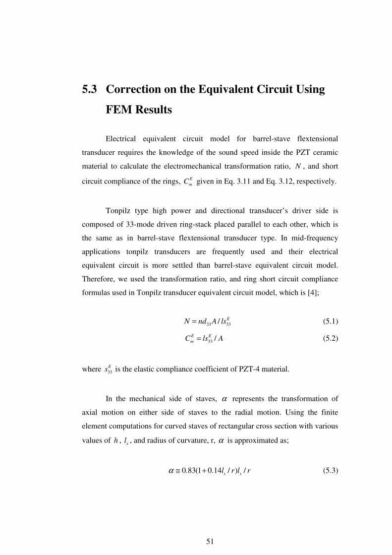
We have changed the shell material from aluminum to carbon/fiber
epoxy. Using the material properties for carbon fiber epoxy given in Appendix I
we obtain the results listed in Table 6.
Design Parameter Description Value
r Radius of curvature of shelf profile 0.08m
t Shell thickness 5mm
l Length of device between end plates 8cm
re Radius at end of device 40mm
hp Thickness of end plate 10mm
ri Inner radius of the ceramic stack 12.7mm/2
ro Outer radius of the ceramic stack 38.1mm/2
D4
n Number of staves forming the shell 8

45
f Fundamental Resonance Frequency 4950 Hz
B Bandwidth 1700 Hz
Q Q-factor 2.91
Table 6 Structural design parameter values and in-water performance characteristics of the staved shell transducer for carbon/fiber epoxy shell element
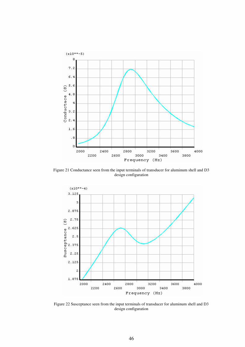
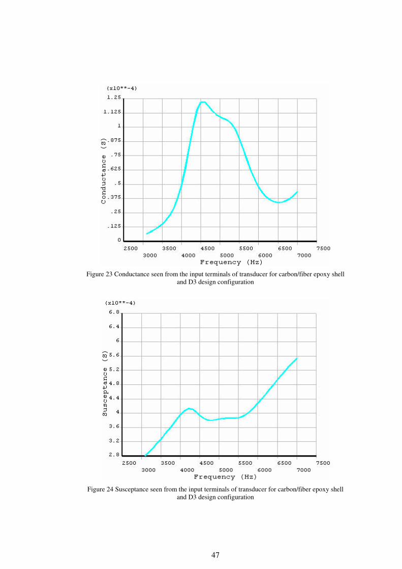
For aluminum shell configuration and D3 structural parameter set given
in Table 5, the conductance and susceptance seen from the input terminals are
obtained as in Figure 21 and Figure 22, respectively and for carbon/fiber epoxy
shell configuration and D4 structural parameter set given in Table 6, the
conductance and susceptance seen from the input terminals are obtained as in
Figure 23 and Figure 24, respectively.
Shell material properties have significant effect on the acoustical
performance of the transducer. The ideal material for low frequency application
must have a low stiffness and a high density, whereas for low quality factor
applications the ideal material must have a high stiffness and a low density [7].
Carbon/fiber epoxy shell yields low quality factor, and high resonance
frequency, whereas aluminum shell yields somewhat higher quality factor, and
lower resonance frequency.
Production of carbon/fiber epoxy is more sophisticated, and needs higher
quality production process compared to aluminum. Therefore, we choose to
produce the aluminum shell design with the structural parameters given in D3 in
Table 5.
For aluminum shell configuration and D3 structural parameter set given
in Table 5, the vacuum conductance and susceptance seen from the input
terminals are obtained as in Figure 25 and Figure 26. SPL of the transducer is
given in Figure 27, which corresponds to the maximum power of 232W.
46
Figure 21 Conductance seen from the input terminals of transducer for aluminum shell and D3 design configuration
Figure 22 Susceptance seen from the input terminals of transducer for aluminum shell and D3 design configuration
47
Figure 23 Conductance seen from the input terminals of transducer for carbon/fiber epoxy shell
and D3 design configuration
Figure 24 Susceptance seen from the input terminals of transducer for carbon/fiber epoxy shell
and D3 design configuration

48
Figure 25 Vacuum Conductance seen from the input terminals of transducer for aluminum shell
and D3 design configuration
Figure 26 Vacuum Susceptance seen from the input terminals of transducer for aluminum shell
and D3 design configuration

49
Figure 27 Source pressure level of barrel-stave transducer obtained from FEM analysis
Normalized directivity functions of barrel-stave flextensional transducer
at resonance frequency in horizontal and vertical plane are given in Figure 28
and Figure 29, respectively. Pressure values that are obtained at 0.5m distant
from the center of transducer are transferred to 1m using spherical spreading
rule. Directivity functions are obtained from the normalized source pressure
levels vs. direction plots. Directivity functions in both planes demonstrate that
the transducer is omnidirectional. This result is expected since the transducer is
small compared with the wavelength at resonance frequency.

50
Figure 28 Normalized horizontal directivity pattern of barrel-stave transducer at resonance
frequency
Figure 29 Normalized vertical directivity pattern of barrel-stave transducer at resonance
frequency
51
5.3 Correction on the Equivalent Circuit Using
FEM Results
Electrical equivalent circuit model for barrel-stave flextensional
transducer requires the knowledge of the sound speed inside the PZT ceramic
material to calculate the electromechanical transformation ratio, N , and short
circuit compliance of the rings, E
mC given in Eq. 3.11 and Eq. 3.12, respectively.
Tonpilz type high power and directional transducer’s driver side is
composed of 33-mode driven ring-stack placed parallel to each other, which is
the same as in barrel-stave flextensional transducer type. In mid-frequency
applications tonpilz transducers are frequently used and their electrical
equivalent circuit is more settled than barrel-stave equivalent circuit model.
Therefore, we used the transformation ratio, and ring short circuit compliance
formulas used in Tonpilz transducer equivalent circuit model, which is [4];
33 33/ EN nd A ls= (5.1)
33 /E E
mC ls A= (5.2)
where 33E
s is the elastic compliance coefficient of PZT-4 material.
In the mechanical side of staves, α represents the transformation of
axial motion on either side of staves to the radial motion. Using the finite
element computations for curved staves of rectangular cross section with various
values of h , s
l , and radius of curvature, r, α is approximated as;
0.83(1 0.14 / ) /s s
l r l rα ≅ + (5.3)

52
which is valid for aluminum staves with / 0.1s
h l ≤ and 0.2 / 1s
l r≤ ≤ . For our
structural dimensions the / 0.0596s
h l = and / 1.0488s
l r = , which is outside the
approximation set. Therefore, we have calculated α using the FEM results.
α is calculated as;
( )
( )
2e average
m rms
ξα
ξ= (5.4)
where
:e
axial displacementξ
:m
radial displacementξ
and the rms and average displacements are calculated as in Eq. 3.7 and Eq. 3.8,
respectively.
α is calculated using the displacement values on one of eight staves
shown in Figure 30. Average axial displacement is calculated from the top 5
nodes’ displacement values in z-direction, and rms radial displacement is
calculated from the 30 nodes’, not including the top 2 row of nodes,
displacement values in radially outward direction. Using the average axial
displacement and rms radial displacement values calculated using Eq. 3.7 and
Eq. 3.8, α values at the frequency range of interest are calculated using Eq. 5.4
and found as in Figure 31.

53
Figure 30 Nodes located on stave that are used to calculate α and β
2000 2200 2400 2600 2800 3000 3200 3400 3600 3800 40000.4
0.45
0.5
0.55
0.6
0.65
0.7
0.75
Frequency (Hz)
Alfa
Figure 31 Alfa vs. Frequency obtained using the FEM results

54
β is the transformation of rms displacement to average displacement on
staves in the radial direction and calculated as;
( )
( )
m rms
m average
ξβ
ξ= (5.5)
where
:m
radial displacementξ
β is calculated using the displacement values on one of eight staves
shown in Figure 30. Radial displacement is calculated from the 30 nodes’, not
including the top 2 row of nodes, displacement values in x-direction. β values
at the frequency range of interest are calculated using Eq. 5.5 and found as in
Figure 32.
2000 2200 2400 2600 2800 3000 3200 3400 3600 3800 4000
1.12
1.13
1.14
1.15
1.16
1.17
1.18
1.19
1.2
Frequency (Hz)
Be
ta
Figure 32 Beta vs. Frequency obtained using the FEM results

55
The radiation impedance of the barrel-stave transducer used in the model
is derived from the radiation impedance of a spherical radiator given as in Eq.
5.6 and in the frequency range of interest the 0 0/Z cρ is given in Figure 33
[17].
2 2
0 0 2 2 2 21 1Sphere
k r krZ Area c j
k r k rρ
= × + + +
(5.6)
0.1 0.2 0.3 0.4 0.5 0.6 0.7 0.8 0.90
1
2x 10
4
Re
(Z)/
(rh
o*c
o)
ka0.1 0.2 0.3 0.4 0.5 0.6 0.7 0.8 0.9
0
1
2x 10
4
Im(Z
)/(r
ho
*co
)
Radiation Impedance
Figure 33 Spherical radiation impedance used in barrel-stave equivalent circuit
Using the obtained α and β values at resonance frequency from the
FEM analysis in equivalent circuit model, and putting the transformation ratio
and ring short circuit compliance formulas in Eq. 5.1 and Eq. 5.2, the vacuum
and in-water conductance-susceptance of electrical equivalent circuit is obtained
as in Figure 34 and Figure 35, respectively.

56
2 3 4 5 6 7-1
0
1
Co
nd
ucta
nce
(S
)
Frequency (kHz)2 3 4 5 6 7
-0.2
0
0.2
Su
sce
pta
nce
(S
)
Alfa = 0.57, Beta = 1.146
Figure 34 Vacuum conductance-susceptance seen from the electrical terminals obtained from equivalent circuit analysis
1 1.5 2 2.5 3 3.5 4 4.5 50
0.2
0.4
0.6
0.8
1
1.2x 10
-4
Co
nd
ucta
nce
(S
)
Frequency (kHz)1 1.5 2 2.5 3 3.5 4 4.5 5
2
4
6
8
10
12
14x 10
-5
Su
sce
pta
nce
(S
)
Alfa = 0.57, Beta=1.146
Figure 35 In-water conductance-susceptance seen from the electrical terminals obtained from equivalent circuit analysis

57
Modifying the electrical circuit results enhances the accuracy of the
equivalent circuit; however, there is still a slight difference between the
admittance obtained from the FEM and equivalent circuit. The electrical circuit
model ignores significant amount of parameters that are considered to have a
little effect on the performance of the transducer. However, FEM well
approximates the real results so it is more precise. Therefore, the slight
difference between the electrical circuit and the FEM results is expected.
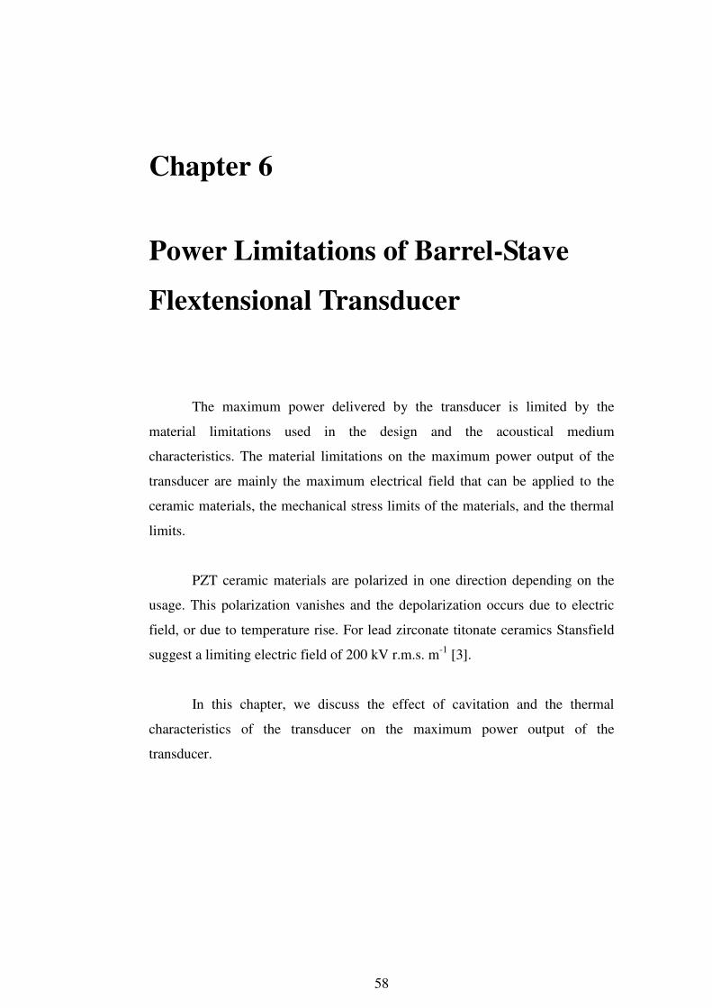
58
Chapter 6
Power Limitations of Barrel-Stave
Flextensional Transducer
The maximum power delivered by the transducer is limited by the
material limitations used in the design and the acoustical medium
characteristics. The material limitations on the maximum power output of the
transducer are mainly the maximum electrical field that can be applied to the
ceramic materials, the mechanical stress limits of the materials, and the thermal
limits.
PZT ceramic materials are polarized in one direction depending on the
usage. This polarization vanishes and the depolarization occurs due to electric
field, or due to temperature rise. For lead zirconate titonate ceramics Stansfield
suggest a limiting electric field of 200 kV r.m.s. m-1 [3].
In this chapter, we discuss the effect of cavitation and the thermal
characteristics of the transducer on the maximum power output of the
transducer.
59
6.1 Cavitation Limitation for Barrel-Stave
Flextensional Transducer
The acoustic power intensity of the sound wave is defined as;
20
2
pI
cρ= (6.1)
As the acoustic power intensity increases, the acoustic pressure increases
and in some point it reaches the hydrostatic pressure of the water. If the intensity
is increased still further, the acoustic pressure peaks will exceed the hydrostatic
pressure of water, and absolute pressure becomes negative at the negative cycle
of the acoustic pressure, so cavitation occurs. When the water medium begins to
cavitate, the bubbles occur in front of the transducer at the negative cycle of the
acoustic pressure cycle [3].
Cavitation causes many undesirable effects on the acoustical
performance of the transducer. Firstly, creation of the bubbles causes additional
power dissipation, and hence reduces the electro-acoustic efficiency. Secondly,
bubbles reduce the acoustical radiating from the transducer. And thirdly, bubbles
disturb the linearity of the medium and causes non-linearity in the radiated
acoustic pressure wave [3].
Formation of bubbles is a nucleation process and it takes some time. As
the frequency of the pressure wave increases, period of negative pressure
decreases so the cavitation threshold increases. Also, decreasing the pulse
length can increase the cavitation threshold.
60
As the depth increases, the ambient pressure also increases, and the
cavitation threshold increases. Urick defines the cavitation threshold at depth h
as [2];
2
0.3 (0)10
c c
hI Pγ
= +
(6.2)
For circular piston, plane and hemispherical type transducers γ is in the
range of 0.3 and 0.6. In our calculations, we take the worst case, which is
0.3γ = . Therefore, the cavitation threshold becomes as;
2
0.09 (0)10
c c
hI P
= +
(6.3)
where h is the depth in meters, Pc(0) is the cavitation threshold pressure at the
surface.
For low frequency acoustic signals, the cavitation threshold pressure
becomes 1 and increases with frequency as illustrated in Figure 36. Therefore,
for f = 3 kHz, the cavitation threshold becomes;
2
0.09 110
c
hI
= +
(6.4)

61
Figure 36 Frequency dependence of cavitation threshold [2]
The maximum continuous wave acoustic power, Pc, that a transducer can
radiate at the onset of cavitation is given by;
( )c cP I h A= (6.5)
where A is the radiating surface area of transducer.
Radiating surface area of barrel-stave transducer is 143 cm2. Therefore,
the maximum acoustic wave acoustic power at the onset of cavitation, Pc, with
respect to depth is calculated as in Figure 37. Delivery of the maximum power
output of the barrel-stave transducer, which is 232 W requires depths more than
33m.

62
0 50 100 150 200 250 3000
2000
4000
6000
8000
10000
12000
14000
Depth (m)
Po
we
r (W
)
Cavitation Power Limit of Barrel-Stave Transducer
Figure 37 Maximum continuous wave acoustic power of barrel-stave transducer at the onset of
cavitation
6.2 Thermal Analysis of Barrel-Stave
Flextensional Transducer
The dielectric and mechanical losses result in the generation of heat
inside the ceramic material. This heat energy causes the rise in the temperature
of the transducer. After a certain temperature limit, called a curie point, PZT
materials loose their piezoelectric properties. The Curie temperature for PZT-4
ceramics is 328 °C [18]. Temperature rise is encountered the most in high duty-
cycle or continuous wave (CW) operations [7]. In practical applications PZT
ceramic temperature aimed to keep well below the Curie temperature, like the
half of the Curie temperature point.
In this section, we determine the behavior of the barrel-stave transducer
at the electrical limiting voltage of continuous 1796 Vp in vacuum and water

63
with coating and without coating materials. In addition, we examine the
thickness of the coating material on the thermal performance of the transducer.
Thermal analysis of barrel-stave transducer is performed using Flux2D
FEM program with the thermal material properties given in Appendix IV. The
FEM model formed in Flux2D program is shown in Figure 38.
Figure 38 FEM model of Barrel-Stave transducer in Flux2D
Power loss inside the PZT materials is given by Şahin as [19];
2 tandP wE Vε δ= (6.6)
where w is the angular frequency of driven electrical signal, E is the electrical
field created inside the PZT rings by the input voltage, V is the total PZT
volume, ε is the dielectric constant of PZT rings, and tanδ is the loss factor.
ALUMINUM
AIR
STEEL
PZT-4 RINGS
EPOXY

64
In order to take the worst case into consideration, we take the frequency
as the upper band frequency that is 3500 Hz, and the electric field as 2000 V/cm.
Dependence of the loss factor and the electric field given in Figure 39 [18], and
we take the loss factor as 0.02.
Figure 39 Loss factor vs. rms electric field [18]
In-air steady state and transient temperature response of the barrel-stave
transducer are given in Figure 40 and 41, respectively. Transducer temperature
reaches steady state at 12000 second and the maximum temperature measured at
the center of the transducer is 131 °C.
65
Figure 40 Steady state temperature distribution of barrel-stave transducer in air
Figure 41 Transient temperature response of barrel-stave transducer taken from the mid point of
the model
66
The convection coefficient of water is approximately the 80 times larger
than air, so we expect to obtain lower steady state temperature in water. Steady
state and transient temperature response of the barrel-stave transducer in water
are given in Figure 42 and 43, respectively. Transducer temperature reaches
steady state at 10000 second and the maximum temperature measured at the
center of the transducer is 62 °C.
Figure 42 Steady state temperature distribution of barrel-stave transducer in water

67
Figure 43 Transient temperature response of barrel-stave transducer in water taken from the mid point of the model
For preventing the water ingression from the gaps between the staves,
barrel-stave transducer must be coated with a material. This material affects the
temperature response of the transducer depending on its thickness and thermal
conductivity properties. We have carried out our analysis with the polyurethane
coating material having a thermal conductivity 0.2 W/m°K for 3 mm and 5 mm
thickness values.
Steady state and transient results obtained for 3 mm coating is given in
Figure 44 and Figure 45, and for 5 mm coating Figure 46 and Figure 47,
respectively. For 3 mm coating, we obtain a maximum 68 °C steady state
temperature, and for 5 mm coating, we obtain a maximum 70 °C steady state
temperature. This temperature levels are well below the Curie point, therefore
we conclude that the temperature is not a power limiting factor for our barrel-
stave transducer.

68
Figure 44 Steady state temperature distribution of barrel-stave transducer in water with 3 mm polyurethane coating
Figure 45 Transient temperature response of barrel-stave transducer in water with 3 mm polyurethane coating taken from the mid point of the model

69
Figure 46 Steady state temperature distribution of barrel-stave transducer in water with 5 mm polyurethane coating
Figure 47 Transient temperature response of barrel-stave transducer in water with 3 mm polyurethane coating taken from the mid point of the model

70
Chapter 7
Experimental Work
In previous chapters we have discussed the design methods and
parameters of barrel-stave flextensional transducer. Using those parameters we
have found a design set which has a low quality factor and frequency. This
chapter deals with the construction and measurement of designed transducer.
In section 7.1 the construction details of transducer are illustrated. The
measured results and comparison of measured results with the theoretical results
are described in section 7.2.
7.1 Construction Details of Barrel-Stave
Flextensional Transducer
The detailed mechanical drawings of transducer structural elements are
given in Appendix V.
The construction of transducer is conducted in three main steps for
controlling the construction and results. After each main step we have compared
the measured and theoretical results.
We have used the 0.7mm %96 alumina instead of MACOR, which has
higher stiffness, higher density and better electrical insulation properties. The

71
material properties of alumina are illustrated in Appendix I and the dielectric
strength of alumina is 9 kV/mm. We have used stainless steel between the
alumina and end-plates to maintain the designed length of barrel-stave
transducer. The cross-section view of transducer is illustrated in Figure 48.
Figure 48 Cross-sectional view of barrel-stave transducer

72
Before we have glued the components, we have constructed the
transducer applying the vaseline between each of the components and test the
transducer in air. Measurements are taken for the transducer without the
aluminum staves and with the aluminum staves, and compared these results with
the theoretical results as shown in Appendix VI.
Afterwards, we have constructed the ceramic stack with end-plates and
glue them. The photograph of the constructed assembly is depicted in Figure 49.
Figure 49 Barrel-stave transducer without aluminum staves
After construction we have applied pre-stress on the ceramic stack. For
the most difficult operating condition of 150 m depth and 1796 V applied
voltage we have obtained the maximum displacement, ∆l , on ceramic material
as 1.57 µm and corresponding strain, S , value to this displacement is calculated
as;

73
4/ 1.574 / 6.35 2.5 10S m mmµ −= ∆ = ≅ ×l l (7.1)
where l is the thickness of one PZT-4 ceramic ring.
After that, we have calculated the stress value using the calculated strain
and young’s modulus of PZT-4 ceramic as;
9 4193 10 2.5 10 48.25T E S MPa−= × = × × × = (7.2)
Total charge generated on ceramic ring is calculated using the
piezoelectric constant, 33d , ring electroded area, A, and the stress obtained in
Eq. 7.2 as;
12 6 333 289 10 48.25 10 10 14Q d TA Cµ− −= = × × × × ≅ (7.3)
Using this charge, the voltage created on the ceramic ring is calculated
as;
1415.56
0.9
Q CV kV
C nF
µ= = = (7.4)
where C is the input capacitance of the ceramic ring.
We have measured the voltage on the ceramic rings using 10M Ω
voltmeter, and used additional capacitor of 6 Fµ in parallel to ceramic rings.
Therefore, the voltage drops to 2.53V V= , and the RC time constant increases
to 1 minute, which is enough to pre-stress and read the voltage on the voltmeter.

74
In second step we glued the aluminum stave to the constructed structure
in step 1. The photograph of the transducer assembly with staves is depicted in
Figure 50.
Figure 50 Barrel-stave transducer with aluminum staves
Lastly, we have sealed the transducer using the silicon material. The
photograph of the final transducer assembly is depicted in Figure 51.

75
Figure 51 Barrel-stave transducer sealed with silicon
7.2 Measured Results of Barrel-Stave
Flextensional Transducer
The in-air measured admittance of transducer without aluminum staves
is obtained as in Figure 52. We obtain the 10.65 kHz measured resonance
frequency which is well approximates to the resonance frequency obtained in
numerical result which is 10.7 kHz.
76
Figure 52 Measured in-air input admittance of transducer without aluminum staves
The in-air measured admittance of transducer with aluminum staves is
obtained as in Figure 53. We obtain the 4.73 kHz measured resonance frequency
which is well approximates to the resonance frequency obtained in numerical
result which is 5 kHz.
77
3 3.5 4 4.5 5 5.5 6 6.5 70
0.5
1
1.5
2
2.5x 10
-3
Co
nd
uc
tan
ce
Me
asu
red
(S
)
Frequency (kHz)
3 3.5 4 4.5 5 5.5 6 6.5 7-1
-0.5
0
0.5
1
1.5x 10
-3
Su
sc
ep
tan
ce
Me
asu
red
(S
)
Figure 53 Measured in-air input admittance of transducer with aluminum staves
Admittance measurement is conducted in 2m x 2m and 1.5m deep water
tank locating in ASELSAN as shown in Figure 54. We have used burst signal
type rather than continuous to decrease the effects of reflections. Measurements
are taken using the program written in Agilent VEE. Measurements are tried to
be conducted in the steady state region of transducer. Transducer reaches its
steady state depending on its quality factor. Barrel-stave transducer’s quality
factor is 3.32 that mean transducer needs approximately 3.5 wavelengths to
reach steady state. At frequency of 1.5 kHz this corresponds to 3.5m, and at
frequency of 3 kHz this corresponds to 1.75m. Our measurement tank is not big
enough to get the data in steady state region before the reflections reach the
transducer. Therefore, we expect to get erroneous data from the water tank
measurements.

78
Figure 54 Water tank with dimensions 2mX2m and 1.5m deep.
Figure 55 and Figure 56 illustrates the comparison of ANSYS and measured in-
water conductance and susceptance of transducer, respectively.
2000 2500 3000 3500 40000
1
2
3
4
5
6
7
8x 10
-5
Frequency (Hz)
Co
nd
ucta
nce
(S
)
Measured Conductance vs ANSYS Conductance
Measured Results
ANSYS Results
Figure 55 In-water conductance measured in water tank vs. conductance obtained in ANSYS

79
2000 2500 3000 3500 40001.6
1.8
2
2.2
2.4
2.6
2.8
3
3.2x 10
-4
Frequency (Hz)
Su
sce
pta
nce
(S
)
Measured Susceptance vs ANSYS Susceptance
Measured Results
ANSYS Results
Figure 56 In-water susceptance measured in water tank vs. susceptance obtained in ANSYS
Conductance and susceptance plot obtained by water tank measurements
illustrates that reflections affect the results significantly. Therefore, interpreting
and comparing the measured results with theoretical results obtained in ANSYS
are insignificant in terms of the performance of transducer.
We have repeated the in-water admittance measurement of transducer in
water-reservoir inside the Bilkent University between the Main Campus and
East Campus as shown in Figure 57. We placed the measurement set up
consisting LCR-8101 impedance analyzer, laptop, 2 x 12Vdc accumulators and 1
x 24V-220Vac inverter to feed the electronic equipments. We have taken the
measurement where the depth is 3m and distance from the shore is 5m. The
bottom of the reservoir is mud that has low reflectivity. Figure 58 and Figure 59
illustrates the comparison of ANSYS and measured in-water conductance and
susceptance of transducer taken in reservoir, respectively.

80
Figure 57 Reservoir inside Bilkent University
2000 2500 3000 3500 40000
1
2
3
4
5
6
7
8x 10
-5
Frequency (Hz)
Co
nd
ucta
nce
(S
)
Measured Conductance vs ANSYS Conductance
Measured Results
ANSYS Results
Figure 58 In-water conductance measured in reservoir vs. conductance obtained in ANSYS

81
2000 2500 3000 3500 40001.4
1.6
1.8
2
2.2
2.4
2.6
2.8
3
3.2x 10
-4
Frequency (Hz)
Su
sce
pta
nce
(S
)
Measured Susceptance vs ANSYS Susceptance
Measured Results
ANSYS Results
Figure 59 In-water susceptance measured in reservoir vs. susceptance obtained in ANSYS
We have reduced the effects of reflection and greatly increased the
reliability of measurements by conducting the measurements in reservoir. We
obtain the 2.82 kHz measured resonance frequency where the theoretical
resonance frequency is 2.92 kHz. However, measured conductance at resonance
frequency is 38 µS where the theoretical conductance at resonance frequency is
72 µS. Conductance of transducer is proportional with the square of the
piezoelectric constant, 33d , as ;
233( )G d∝ (7.5)
Ratio of measured conductance and theoretical conductance is;
380.53
72measured
theoratical
G S
G S
µ
µ= ≅ (7.6)

82
Therefore, the ratio of the piezoelectric coefficient with the one we use
in theoretical calculations is the square root of the value obtained in Eq. 7.6 ,
which is 0.73.
33
33
0.53 0.73measurement
datasheet
d
d= = (7.7)
Piezoelectric rings that we have used are more than twenty years and
change in the piezoelectric coefficient found as in Eq. 7.7 is reasonable. Other
possibility is that the original piezoelectric coefficient value of those rings might
be lower than the present piezoelectric coefficient value.
Blocked capacitance, Cb, of transducer is calculated as
02b
BC
fπ= (7.8)
where B is susceptance at resonance frequency and f0 is the resonance
frequency.
The theoretical and experimental results are summarized in Table 7.
Parameter Theoretical Results Experimental Results
f0,air 5 kHz 4.73 kHz
f0,water 2.92 kHz 2.82 kHz
BWwater 880 Hz 215 Hz
Qwater 3.32 4.3
Gmax 72 µS 38 µS
Cb 13.6 nF 11.7 nF
Table 7 Theoretical Results vs. Measured Results

83
Chapter 8
Conclusion
The need for the detection of targets from long distances increases the
importance of high power and low frequency transducer. In this thesis, the
design of barrel-stave flextensional transducer is reported.
Comparison of the equivalent circuit results of barrel-stave transducer
with the Bayliss’s FEM results illustrated the inconsistency between the FEM
and equivalent circuit results, so design of transducer is done using FEM.
The finite element method is used to investigate the electro-acoustic
behavior of barrel-stave transducer with high accuracy, although
computationally intensive.
Among eight design parameters of barrel-stave transducer, we have
optimized the transducer performance with low Q-factor using five structural
parameters which are; radius of curvature of shell profile, r, shell thickness, t,
length of device between end plates, l, radius at end of device, re, thickness of
end plate, hp. We have used the PZT-4 rings that we have in hand, so we were
somewhat limited in design.
Low frequency and low quality factor requirement is accomplished with
D3 design parameter set given in Table 5. We have acquired much lower quality
factor and relatively larger power level compared to the scaled version of
Bayliss’s slotted-shell design.

84
Thereafter, some of equivalent circuit elements are modified using the
FEM results and it is illustrated that the modified circuit results are compatible
with the FEM results.
Power limitations of barrel-stave flextensional transducer are examined
in terms of electrical limitations, cavitation, and thermal limitations. Cavitation
and thermal analysis are carried out by applying the voltage creating the electric
field limit of 2000 V/cm. Cavitation threshold limits the power up to a depth of
33 meters. Thermal analysis is carried out for various combinations including
the coating of transducer and we have found that our design is not a thermally
power limited. Consequently; up to 33 meters, cavitation limits the acoustic
power of barrel-stave transducer and after this depth, maximum electric field
applied to ceramic materials before depolarization limits the acoustic power.
Vacuum measurements agree well with the FEM results; however, we
face some difficulties in in-water measurements. Water tank is small compared
to our desired amount of wavelengths in order not to take reflections. Therefore,
conductance and susceptance plot obtained by water tank measurements
illustrates that reflections affect the results significantly. We have repeated the
in-water measurements of transducer in water-reservoir inside the Bilkent
University and reduced the effects of reflection and greatly increased the
reliability of measurements.
As a future work, more experimental work would be to carry out to
obtain the entire acoustic characteristics of transducer. In addition, array
formation using barrel-stave flextensional transducer could be studied.

85
Appendix I
The ‘base’ values of the structure’s dimensions and the material properties
Parameter Description Base Value
r Radius of curvature of shell profile 0.25m
t Shell thickness 15mm
l Length of device between end plates 25cm
re Radius at end of device 85mm
hp Thickness of end plate 30mm
ri Inner radius of the ceramic stack 20mm
ro Outer radius of the ceramic stack 40mm
n Number of staves forming the shell 12
Table 8 Structural parameters and their base values
Part Material Density
(kg m-3)
Young’s
modulus
(GPa)
Poisson’s
ratio
Ceramic PZT-4
Insulator MACOR 2520 140.0 0.29
End-plate Steel 7960 193.0 0.31
Shell Aluminum 2710 68.91 0.30
Glue joints Araldite 1180 6.5 0.40
Table 9 Material Properties used in Clive Bayliss Thesis

86
Part Material Density
(kg m-3)
Young’s
modulus
(GPa)
Poisson’s
ratio
Shell Carbon/Fiber
Epoxy 1800 225 0.33
Insulator %96 Alumina 3800 300 0.22
Table 10 Carbon/Fiber Epoxy and Alumina Material Properties
87
Appendix II
Effective Vibrating Mass of Stack
Figure 60 Basic static and end mass
Figure 60 shows the basic static and end mass configuration of
transducer. Assume that the displacement of the stack is approximately
proportional to its distance from the nodal plane. The displacement velocity of
the element xδ at a distance x from the node is approximately /vx L , where L
is the total length of the stack and v is the velocity of the end mass M . When
the static mass of the static mass of the stack is s
M , the mass of the element is
/s
M x Lδ . The kinetic energy of the system is written as;
( )
2
2
20
1
2
L
sk
vxME Mv dx
L L
= +
∫ (II-1)

88
2 32
2
1
2 3s
k
M v LE Mv
L L
= +
(II-2)
221
2 3s
k
M vE Mv
= +
(II-3)
21
2 3s
k
ME M v
= +
(II-4)
Therefore, the effective vibrating mass of the stack is 3s
M , which is
added to the end masses in the equivalent circuit equations [3].
89
Appendix III
Element Types Used in the ANSYS Model
Element type entry window in ANSYS is illustrated in Figure 61.
Figure 61 Element type selection window in ANSYS
Material Matrices for PZT-4
Density of PZT-4 element is;
37500 /kg mρ =
For +Z and –Z polarized PZT-4 rings Dielectric matrix, and Stiffness
matrix coefficients are the same and given as;

90
PZT-4 Dielectric Matrix [ rε ]:
730 0 0
0 730 0
0 0 635
PZT-4 Stiffness matrix [c] x GPa
139 77.8 74.3 0 0 0
139 74.3 0 0 0
115 0 0 0
30.6 0 0
25.6 0
25.6
PZT-4 Piezoelectric Matrix coefficients change its sign as it changes its
polarization direction from +Z to –Z direction as;
+Z polarized PZT-4 Piezoelectric Matrix [e] 2/C m
0 0 5.2
0 0 5.2
0 0 15.1
0 0 0
0 12.7 0
12.7 0 0
− −
-Z polarized PZT-4 Piezoelectric Matrix [e] 2/C m
0 0 5.2
0 0 5.2
0 0 15.1
0 0 0
0 12.7 0
12.7 0 0
− − −

91
Appendix IV
Thermal Properties of Materials
Thermal properties of materials that are used in thermal analysis are
given in Table 11.
Material Thermal
Property Value Unit
Thermal
Conductivity 1.8 W/m°K
PZT-4
Specific Heat 3192000 J/m3°K
Thermal
Conductivity 54 W/m°K
Steel
Specific Heat 3744000 J/m3°K
Thermal
Conductivity 237 W/m°K
Aluminum
Specific Heat 2422000 J/m3°K
Thermal
Conductivity 0.2 W/m°K
Epoxy
Specific Heat 2562000 J/m3°K
Thermal
Conductivity 0.2 W/m°K
Polyurethane
Specific Heat 88000 J/m3°K
Water Convection
Coefficient 1350 W/m2°K
Air Convection
Coefficient 22 W/m2°K
Table 11 Thermal properties of materials

92
Appendix V
Construction Details of Barrel-Stave Transducer
The cross-section view of transducer is illustrated in the first drawing.
Components
8 x PZT-4 rings
8 x Aluminum Stave
1 x Stainless Steel Endplate without holes (Endplate I)
1 x Stainless Steel Endplate with 2 holes (Endplate II)
2 x Alumina Insulator
2 x Stainless Steel Washer
9 x Copper Berilium Conductor Sheet
1 x Stainless Steel Center Bolt
Adhesives
Ecobond 45 Clear and Catalyst 15 Clear mixed 1:1 ratio for rigid gluing
and applied between PZT rings, conductor sheets, insulators and washers
(Emerson & Cuming)
We have applied epoxy / polyamide adhesive with ratio of 1:1 between
the endplates and aluminum staves. The adhesive is the product of Tyco
Raychem with type number of S1125-KIT-8.
Other Materials
16 x (M4x10) cross necessed countersunk (flat) head screw
3 x M10 Hexagon Nut
Single core silicon insulated cable with1500V rating.


102
Appendix VI
Measured Results for Transducer constructed with Petrolatum
Transducer structure is tested in two steps before applying glue to
components in order to find out if there is an inconsistency between the
theoretical and measured results.
The in-air measured admittance of transducer without aluminum staves
is obtained as in Figure 62. Measured resonance frequency is 9.5 kHz and the
numerical resonance occurs at 10.7 kHz.
7 8 9 10 11 12 130
0.5
1
1.5
2
2.5
3
3.5
4x 10
-3
Co
nd
uc
tan
ce
Me
asu
red
(S
)
7 8 9 10 11 12 13-1.5
-1
-0.5
0
0.5
1
1.5
2
2.5x 10
-3
Su
sc
ep
tan
ce
Me
asu
red
(S
)
Frequency (kHz)
Figure 62 Measured in-air input admittance of transducer without aluminum staves
103
The in-air measured admittance of transducer with aluminum staves is
obtained as in Figure 63. Measured resonance frequency is 4.12 kHz and the
numerical resonance frequency is 5 kHz.
We have obtained lower resonance frequency for both measurements.
ANSYS model simulates the contacts between the mechanical elements of
transducer as strictly bonded, which are proper for the glued case. However, in
this case we have used vaseline instead of glue, which decreases the stiffness of
transducer structure and also decreases the resonance frequency.
Figure 63 Measured in-air input admittance of transducer with aluminum staves

104
BIBLIOGRAPHY
[1] X. Lurton, An Introduction to Underwater Acoustics Principles and
Applications. Springer, 2002
[2] Robert J. Urick, Principles of Underwater Sound 3rd
Edition. McGraw-Hill
Book Company, 1983.
[3] D. Stansfield, Underwater Electroacoustic Transducers. Bath, UK: Bath
Univ. Press, 1990.
[4] Charles H. Sherman and John L. Butler, Transducers and Arrays for
Underwater Sound. Springer, 2007.
[5] James R. Phillips, “Piezoelectric Technology Primer”
[6] ANSYS, Piezoelectrics, Release 11.0 Documentation for ANSYS, 11.3.
[7] Clive Bayliss, Application and Development of Finite Element Techniques
for Transducer Design and Analysis, University of Birmingham, 1998.
[8] Meet the Finite Element Method,
media.wiley.com/product_data/excerpt/89/04713707/0471370789.pdf
[9] D. Roylance, Finite Element Analysis, Massachusetts Institute of
Technology, 2001.
[10] V. Piefort, A. Preumont, Finite Element Modeling of Piezoelectric
Structures, Active Structures Laboratory.

105
[11] William S. Burdic, Underwater Acoustic System Analysis. Prentice-Hall,
1990
[12] D.F. Jones, Flextensional Barrel-Stave Projectors, in Transducers for
Sonics and Ultrasonics, ed. By M.D. McCollum, B.F. Hamonic, and O.B.
Wilson, Technomic Publishing Co, 1993.
[13] J.N. Decarpigny , B. Hamonic and O.B. Wilson, The Design of Low-
Frequency Underwater Acoustic Projectors: Present Status and Future
Trends, IEEE Journal Of Oceanic Engineering, Vol. 16, No. I . , 1991
[14] D.T.I. Francis, C. Bayliss, J.A. Ahmad and R.F.W. Coates, The
Development of a Low Frequency Barrel-Stave Transducer for
Tomographic Applications Using Finite Element and Boundary Element
Modelling, IEEE 0-7803-2056-5, 1994
[15] M.B. Moffett, J.F.Lindberg, E.A. McLaughlin and J.M. Powers, An
equivalent circuit model for barrel stave flextensional transducers, in
Transducers for Sonics and Ultrasonics, ed. By M.D. McCollum, B.F.
Hamonic, and O.B. Wilson, Technomic Publishing Co, 1993.
[16] ANSYS, Release 11.0 Documentation for ANSYS. ANSYS Inc.
[17] David T. Blackstock, Fundamentals of Physical Acoustics, Wiley-
Interscience Publication, 2000.
[18] Properties of Piezoelectric Ceramics, www.morgan-electroceramics.com
[19] Zekeriyya Şahin, The Design Of A Wideband And Widebeam Piston
Transducer In A Finite Closed Circular Baffle, Bilkent University, 2008
Related Documents