Barotropic tides in the South Atlantic Bight

Barotropic tides in the South Atlantic Bight

Brian O. Blanton,1 Francisco E. Werner,1 Harvey E. Seim,1 Richard A. Luettich Jr.,1

Daniel R. Lynch,2 Keston W. Smith,2 George Voulgaris,3 Frederick M. Bingham,4

and Francis Way5

Received 29 April 2004; revised 12 September 2004; accepted 20 October 2004; published 21 December 2004.

[1] The characteristics of the principal barotropic diurnal and semidiurnal tides areexamined for the South Atlantic Bight (SAB) of the eastern United States coast. Wecombine recent observations from pressure gauges and ADCPs on fixed platforms andadditional short-term deployments off the Georgia and South Carolina coasts together withNational Ocean Service coastal tidal elevation harmonics. These data have shed lighton the regional tidal propagation, particularly off the Georgia/South Carolina coast, whichis perforated by a dense estuary/tidal inlet complex (ETIC). We have computed tidalsolutions for the western North Atlantic Ocean on two model domains. One includes afirst-order representation of the ETIC in the SAB, and the other does not include the ETIC.We find that the ETIC is highly dissipative and affects the regional energy balance ofthe semidiurnal tides. Nearshore, inner, and midshelf model skill at semidiurnalfrequencies is sensitive to the inclusion of the ETIC. The numerical solution that includesthe ETIC shows significantly improved skill compared to the solution that does notinclude the ETIC. For the M2 constituent, the largest tidal frequency in the SAB, overallamplitude and phase error is reduced from 0.25 m to 0.03 m and 13.8� to 2.8� forcoastal observation stations. Similar improvement is shown for midshelf stations. Diurnaltides are relatively unaffected by the ETIC. INDEX TERMS: 4219 Oceanography: General:

Continental shelf processes; 4255 Oceanography: General: Numerical modeling; 4560 Oceanography:

Physical: Surface waves and tides (1255); 4223 Oceanography: General: Descriptive and regional

oceanography; KEYWORDS: barotropic tide, South Atlantic Bight, finite element model

Citation: Blanton, B. O., F. E. Werner, H. E. Seim, R. A. Luettich Jr., D. R. Lynch, K. W. Smith, G. Voulgaris, F. M. Bingham, and

F. Way (2004), Barotropic tides in the South Atlantic Bight, J. Geophys. Res., 109, C12024, doi:10.1029/2004JC002455.

1. Introduction and Background

[2] The majority of water level variability in many coastalregions is tidal in origin, and a distinct advantage in tidalprediction is that tidal responses occur at discrete frequenciesdetermined by combinations of astronomical frequencies aswell as frequencies that result from nonlinear interactions inthe governing physics. Harmonic analysis of sufficientlylong observations of water level have been used historicallyfor accurate local prediction of tides. However, mapping thespatial character of the tides requires accurate tidal modelssince observational coverage is generally sparse in the deepocean. Typical skill in the numerical prediction of M2 tidalelevation is 0.05 m and 5� (Foreman et al. [1995] and

Foreman and Thomson [1997] on the northwest Pacificcoast, He and Weisberg [2002] on the west Florida shelf,Davies and Kwong [2000] on the northwest European shelf,Lynch and Naimie [1993] and Naimie et al. [1994] in theGulf of Maine). However, good tidal skill in the SouthAtlantic Bight region of the eastern U.S. coast has beencomparatively elusive [Mukai et al., 2002].[3] We present an analysis of observations in the South

Atlantic Bight (SAB) that includes recent data from a set ofoffshore midshelf towers plus an additional mooring in theGrays Reef National Marine Sanctuary (GR) as well aswater levels from long-term National Ocean Service (NOS)gauge sites. Depth-averaged velocities are also examinedwhere available. Comparison of numerical model results tothe tidal analysis is made, with the goal of determining thebest prior estimate of tidal boundary conditions for limited-area model studies [Lynch et al., 2004; Blanton, 2003].[4] The data most routinely available for data-assimilat-

ing coastal regional forecasting models are typically frompermanent water level gauges in the coastal and nearshorezones. This region can be strongly influenced by tidal inletsand estuaries (as described herein). We have recently shown[Lynch et al., 2004] that assimilation of coastal water levelobservations must be performed with a model that includesthe estuaries and tidal inlets. It is not sufficient to ensure thatthe landward boundary of the model domain encompasses

JOURNAL OF GEOPHYSICAL RESEARCH, VOL. 109, C12024, doi:10.1029/2004JC002455, 2004

1Department of Marine Sciences, University of North Carolina atChapel Hill, Chapel Hill, North Carolina, USA.

2Thayer School of Engineering, Dartmouth College, Hanover, NewHampshire, USA.

3Department of Geological Sciences, University of South Carolina,Columbia, South Carolina, USA.

4Center for Marine Science, University of North Carolina atWilmington, Wilmington, North Carolina, USA.

5Applied Technology and Management, Inc., Charleston, SouthCarolina, USA.

Copyright 2004 by the American Geophysical Union.0148-0227/04/2004JC002455$09.00

C12024 1 of 17

the spatial locations of the water level gauges. A largeportion of the ETIC must be included to properly model theM2 tide. However, tidal dynamics in the SAB region, andthe effects of the estuaries on the shelf-wide tidal character-istics, were not investigated in [Lynch et al., 2004].[5] The South Atlantic Bight region of the eastern United

States coast extends from Cape Hatteras, North Carolina toCape Canaveral, Florida (Figure 1). The continental shelf(shoreward of the 200-m isobath) is 10–30 km wide at thenorthern and southern extremes and broadens to 120 km offthe Georgia coast. Bathymetric contours are parallel to thecoast. The coast is perforated with a complex of estuariesand tidal inlets (henceforth, the estuary/tidal inlet complex,ETIC) from middle South Carolina to northern Florida. TheGulf Stream generally lies seaward of the 100-m isobath.[6] The tidal environment in the SAB is a semidiurnal

(primarily M2) cooscillation with the North Atlantic deepocean tide [Redfield, 1958]. Significant amplification occursalong the widest part of the continental shelf (off Georgia).The tidal velocity ellipse major axes are generally orientedcross-shelf, with minor axes lengths about half that of themajor axis length [Redfield, 1958; Clarke and Battisti,1981; Werner et al., 1993]. The tidal Eulerian residualvelocity is weak, with equatorward shelf break flow and

poleward nearshore flow at about 0.01 m s�1 [Werner et al.,1993]. Tidal contributions to the total water level andcurrent variance are substantial. Tebeau and Lee [1979]and Lee and Brooks [1979] found that the variance in thetidal frequency band accounted for 80–90% and 20–40%of the cross-shelf and along-shelf current variance in themidshelf. Along with Pietrafesa et al. [1985], their resultsalso demonstrated the cross-shelf nature of this variancepartitioning: semidiurnal tides accounted for about 80% ofinner and midshelf kinetic energy, while accounting for onlyabout 30% of outer shelf energy.[7] More specifically, Redfield [1958] considered the M2

elevation and velocity along the Middle Atlantic Bight(MAB) and northern SAB from shelf stations. His analysisstopped at Savannah, Georgia, but indicated that the M2

surface tide is a standing wave on the shelf in the MAB.This suggests that the large-scale coastal water level atsemidiurnal frequencies is in phase along the coast and thatmaximum shoreward tidal velocities lead the time of highwater by about one-quarter period. Redfield found that thiswas also true for the semidiurnal tide on the SAB shelf, atleast as far south as Savannah: M2 progresses slowly alongthe shelf break, and the time of maximum shoreward currentleads the time of maximum water level by about 3 h. He

Figure 1. Study region. The South Atlantic Bight extends from Cape Hatteras, North Carolina, to CapeCanaveral, Florida. Water level stations are shown with squares. ADCP stations are shown with crosses.The 20, 35, 200, 600, 1000, 3000, and 5000-m isobaths are shown. The Bermuda water level station isnot shown on this figure. The box is detailed in the inset. (inset) Close-up of the northern coast ofGeorgia. The 5, 10, 15, 25, and 35-m isobaths are shown.

C12024 BLANTON ET AL.: SOUTH ATLANTIC BIGHT TIDES

2 of 17

C12024

also demonstrated that the M2 tide exhibited the largestcross-shelf amplification at the widest part of the continentalshelf. The M2 elevation at the shelf break of 0.5 m amplifiesto about 1.0 m along the Georgia coast. He concluded thatthe semidiurnal tides along the U.S. east coast are acooscillation with the open ocean North Atlantic tide, beingforced at the shelf break. The character of the tide equator-ward of Savannah was ambiguous.[8] Clarke and Battisti [1981] and Clarke [1991] devel-

oped an analytical treatment describing cross-shelf tidalcharacteristics. They explained semidiurnal elevation am-plification in midlatitude regions by constructive interfer-ence of inertia-gravity waves propagating cross-shelf.Diurnal tides, for which frequencies are near-inertial inthe middle and lower SAB, cannot propagate shorewardas inertia-gravity waves, cannot constructively interfere, andhence do not amplify.[9] Chen et al. [1999] examined inner shelf frontal

mechanisms off the Georgia coast, including a contributionfrom tidal mixing. They provided solutions for the tides on alimited-area model domain that appear reasonable in ampli-tude and phase skill, despite the low resolution of thecoastal zone and the neglect of the tidal inlet energy sinks.However, since the tides were included in this study toprovide a background mixing environment, skill in tideswas not rigorously assessed.[10] Lentz et al. [2001] considered tidal observations in

the lower MAB, from Cape Hatteras north toward theChesapeake Bay entrance. Although geographically outsideof the SAB, their results are of interest because theydescribe the mechanisms behind along-shelf variation inthe semidiurnal tidal velocities. Using data analysis and a 2-D analytical model, along-shelf semidiurnal tidal variationis explained largely by increases in the shelf width fromCape Hatteras to the Chesapeake Bay entrance. The wid-ening shelf induces a weak progressive wave component tothe otherwise standing wave solution, which in turn devel-ops a phase lag near the coast. Variations in diurnal tidalparameters were not sensitive to the primary mechanism intheir analytical model (linearly increasing/decreasing shelfwidth) and are apparently not due to shelf width variations.[11] Energy analyses for global ocean tides, derived from

satellite altimetry and global tidal models [e.g., Kantha etal., 1995], indicate that the bulk of energy input into theoceans occurs in the open ocean, due to lunar and solargravitational loading. This input energy must eventually bedissipated, and a substantial portion is extracted by bottomfriction in shallow marginal seas and on broad continentalshelves (e.g., Yellow Sea [Kang et al., 2002], northwestEuropean shelf [Davies and Kwong, 2000], Patagonianshelf [Glorioso and Flather, 1997]). An additional portionof the input energy (as much as 30% [Egbert and Ray,2000]) now appears to be shunted to the baroclinic tides indeep ocean regions like the Hawaiian Ridge and the Mid-Atlantic Ridge [Kantha and Tierney, 1997; Ray andMitchum, 1997; Munk, 1997; Egbert and Ray, 2000; Kanget al., 2000]. The tidal energy that is transported to the shelffrom the deep oceans is dissipated through the retardingaction of bottom friction that opposes the tidal motion onthe shelf. Part of this dissipation occurs in nearshore regionswhere the tidal flow is enhanced by the presence of tidalinlets and estuaries, as in the SAB.

[12] While the total tidal dissipation on the SAB shelf is asmall fraction of the global tidal power input (�1.8 GWversus �2.4 TW), and in fact a small fraction of the totaldissipation in the North Atlantic Ocean (�0.7 TW), about25% of the dissipation in the SAB occurs in the ETIC alongthe Georgia/South Carolina coast (see Results section).Basin or global scale tidal models typically do not (orcannot) include estuaries and tidal inlets, assuming thattheir effects are localized and do not affect the larger-scalesolutions. We demonstrate that, while this assumption maybe justified, the SAB local and regional tidal solutions atsemidiurnal frequencies are fundamentally influenced bythe ETIC. Since numerical model solutions of the SAB thatare focused on shelf-scale performance (and some that arefocused on inner shelf and nearshore processes) do nottypically include nearshore geometries, it is difficult toaccurately model the barotropic tides in the semidiurnalband with skill that compares to tidal modeling of otherregions.

2. Data and Methods

[13] For this study, water level and velocity observationshave been collected from a variety of sources in the SAB.Water level data sources include the following: bottompressure records from several permanent midshelf deploy-ments from the South Atlantic Bight Synoptic OffshoreObservational Network (SABSOON [Seim, 2000]); tempo-rary deployments in the region; and published water levelharmonic constituents from NOS (Table 1 and Figure 1).These latter stations are generally located within the ETIC,which we broadly define as the wetted region landward ofthe sound limits. Bottom pressure records are converted tosea levels using the standard hydrostatic relationship. Thepublished harmonic constituents from NOS stations areused assuming that they represent the most robust constit-uent estimates, given the long historical record from whichthe constituents are derived.[14] Velocity data are comparatively less available and are

limited to ADCP records from permanent deployments attwo SABSOON tower locations and several short-termdeployments: two in the SABSOON tower region and oneeach in Long Bay and Onslow Bay (Table 2 and Figure 1).The tidal current analysis is limited to the depth-averagedflow.[15] Harmonic analysis of the water level and depth-

averaged ADCP observations was performed using theMATLAB code t_tide [Pawlowicz et al., 2002]. The timespans for the data are not contemporaneous. We have usedthe longest possible record length L at each station, whichvaries from 28 to 851 days. All data records were decimatedto hourly values. We are primarily interested in M2 and K1.However, the Rayleigh frequency separation criterionjDfjL > 1 between K1 and P1 requires a record length of4192 h (about 175 d). Otherwise, the harmonic estimate ofK1 is contaminated with P1 variance. P1 can be inferredfrom K1 if the ratio between the two can be estimated fromrecords of sufficient duration. Using the water level andvelocity harmonic analysis at the tower stations R2 and R6,the amplitude ratio K1/P1 � 3, and the phase difference K1 �P1 � 0. For records shorter than 175 d, we use thisamplitude ratio and phase difference to infer P1, and more

C12024 BLANTON ET AL.: SOUTH ATLANTIC BIGHT TIDES

3 of 17

C12024

appropriately determine K1. This amplitude ratio and phasedifference is consistent for other data locations in the SABfor which long records are available.[16] Numerical solutions in the western North Atlantic

Ocean are computed using ADCIRC-2DDI [Luettich et al.,1992] which solves the vertically integrated, fully nonlinearshallow-water wave equations on linear triangular finiteelements. This model is used in tidal simulations, stormsurge calculations, and sediment transport studies, as well asin the operational oceanographic context [Lynch et al.,2001; Blanton, 2003]. We use a standard quadratic bottomfriction formulation with a drag coefficient of Cd = 0.003and a minimum depth of 4.0 m. The model domain(Figure 2) extends westward from the only open boundary(60�W) and includes the Gulf of Mexico as well as a high-resolution representation of the ETIC along the coasts ofGeorgia, South Carolina, and North Carolina. Figure 2 alsoshows the nearshore detail and resolution in the vicinity ofthe Savannah River entrance. The model grid contains63,076 nodes and 111,748 elements, with horizontal reso-lution ranging from 100 km in deep water, 2–10 km on the

SAB shelf, to 50–100 m in the tidal inlets and estuaries.This latter resolution limits the model time step to 10 s. Werefer to this domain as the ‘‘estuary’’ domain.[17] The bathymetry is a combination of ETOPO5 in deep

water, and NOAA’s Coastal Relief Model on the SAB shelfand in the ETIC. Tidal amplitude and phase is specifiedalong the open boundary, and the tidal potential is specifiedas well. The forcing spectrum is M2, N2, S2, O1 and K1,extracted from the TOPEX-Poseidon altimeter-assimilatedFES95.2 global tidal solutions [Le Provost et al., 1998]. Themodel is integrated for 180 d, and harmonic analysis isperformed at each model node over the second 90 d periodof the integration.[18] To investigate the impact of the ETIC on tides on the

SAB shelf, an additional tidal solution is computed on afinite element domain that does not include the ETIC. Allnodes landward of the sound limits have been removed, andthe resulting new boundary segments are treated as no-normal-flow boundaries. This domain is otherwise the sameas the above-described ‘‘estuary’’ grid and is referred to asthe ‘‘no-estuary’’ grid (Figure 2, inset).[19] Quantitative comparison between observed and mod-

eled elevations is made by computing the complex error Ebetween the values at each station:

E ¼ Aoeifo � Ace

ifc

�� ��

where Ao, Ac and fo, fc are the observed and computedwater level amplitudes and phases, respectively. Root-mean-square (rms) differences between observed and modeledvalues are used to quantify larger-scale error. For the estuarysolution, all observation locations are within the modeldomain. For the no-estuary solution, several water levelstations are outside of the domain. For these stations, thesolution is sampled at the nearest grid location. Modelsolutions are shown primarily for the SAB region. Vectorand ellipse plots are sampled onto a regular grid forvisualization purposes. Elevation, velocity, orientation, andphase are reported in m, m s�1, degrees (�), and Greenwichdegrees (�G). Throughout the remainder of the paper, tablesand figures report observations and model results from bothmodel solutions, each discussed where appropriate.

3. Results

3.1. Observations

[20] The longest midshelf water level record (SABSOONtower R2, Table 3) shows that the main semidiurnalconstituent isM2, followed by N2 and S2. The largest diurnal

Table 1. Water Level Station Locationsa

Station AbbrLongitude,

�WLatitude,

�NDepth,m

RL,days

EstuaryCape Hatteras, NC+ CHat 75.64 35.22 - -Beaufort Inlet, NC BIOS 76.67 34.68 14.6 63Beaufort Inlet, NC+ BI 76.67 34.72 - -Charleston, SC+ Char 79.93 32.78 - -Charleston Entrance, SC CharV 79.78 32.64 14 28Ft. Pulaski, GA+ FtPl 80.90 32.03 - -Georgia Port Auth. GPA01 80.83 32.04 8.5 50D86, Wassaw Sound, 1986 D86 80.95 31.92 4.5 45St Simons Island, GA+ SSI 81.40 31.13 - -Fernandina Beach, FL+ Fern 81.47 30.67 - -St. Johns River, FL+ StJ 81.43 30.40 - -

ShelfOnslow Bay 27, NC OB27 77.30 33.95 35 250Long Bay, NC LB 78.74 33.69 14 39Springmaid Pier, SC + SMPier 78.92 33.66 - -Onslow Bay 63, NC OB63 77.10 33.40 90 77Sav’h Navigational

Light TowerSNLT 80.68 31.95 14 40

D87, FLEX 1987 D87 80.55 31.68 20 45R6 R6 80.23 31.53 35 516R2 R2 80.57 31.38 26 851Gray’s Reef, GA GR 80.92 31.36 16 76R5 R5 80.77 30.93 24 76St. Augustine, FL+ StA 81.26 29.86 - -

DeepBermuda Berm 64.42 32.22 - 365Pearson Pear 76.42 30.43 3766 180

aStations marked with a superscript plus are NOS water level gauges.Abbr is the station abbreviation used in the text and figures. RL is therecord length in days. Stations are grouped according to proximity to theETIC of the Georgia/South Carolina coast. Estuary stations are generallylocated landward of the sound demarcation line (FtPl) or in the immediatevicinity of the coastal zone (e.g., D86). Shelf denotes stations that areoffshore and removed from the immediate influence of tidal inlets/estuarymouths. This includes ‘‘beach’’ stations (e.g., StA) as well as midshelfstations (e.g., R2). Two Deep stations are included. Within each group,stations are listed from north to south. The source of the GPA01observations is Way [1998]. The Bermuda station observations are fromthe Hawaii Sea Level Center, and the source of the Pearson station isPearson [1975]. R2 and R6 are permanent SABSOON installations. GRand R5 are temporary SABSOON deployments.

Table 2. Velocity Station Locations From Which ADCP Records

Are Availablea

Station AbbrLongitude,

�WLatitude,

�NDepth,m

RL,days

Onslow Bay 27 OB27 77.30 33.95 35 671Long Bay, NC LB 78.74 33.69 14 39R6 R6 80.23 31.53 35 913R2 R2 80.57 31.38 26 547Gray’s Reef, GA GR 80.92 31.36 16 76R5 R5 80.77 30.93 24 76

aAbbr is the station abbreviation used in the text and figures. RL is therecord length in days. R2 and R6 are permanent SABSOON installations.GR and R5 are temporary SABSOON deployments.

C12024 BLANTON ET AL.: SOUTH ATLANTIC BIGHT TIDES

4 of 17

C12024

tides are K1 and O1. The published harmonic constituentsfor the NOS stations show that the same semidiurnal anddiurnal frequencies dominate the coastal station tides. Thisis typical of other U.S. east coast regions and has beenreported by others, including Moody et al. [1984]. Theannual and semiannual steric anomaly tides (SA and SSA) arenot small (0.14 m and 0.08 m, respectively). M2 and K1

account for about 92% and 57% of the total semidiurnal anddiurnal variance, respectively.[21] Table 4 reports the observed water level amplitude

and phase for the constituents M2, N2, S2, K1 and O1, andincludes published values for NOS stations. Observed M2

water level amplitudes are largest in the Savannah, Georgia,region (e.g., FtPl, GPA01) at about 1.0 m. Amplitudesdecrease to the north and south, to 0.66 m at St. Augustineand 0.45 m at Cape Hatteras, respectively. Although thereare no directly cross-shelf station sequences, the OnslowBay stations (OB63 and OB27) in the northern part of theregion show typical semidiurnal cross-shelf amplification:from 0.46 m closer to the shelf break (OB63) to 0.55 m atabout midshelf (OB27). This is also seen at the SABSOONtower region, where the amplitude increases from 0.68 m atthe R6 tower to 0.89 m at the GR station.[22] The general equatorward phase propagation of all

constituents is noted. In the cross-shelf direction, all con-

stituents are largely in phase in the northern part of the SAB(OB63, OB27). In the middle SAB region, the M2 phaseincreases shoreward, from 3.0� at R6 to 10� at the GRstation (the latest midshelf value). The latest phases occur at

Table 3. Fifteen Largest Tidal Constituents From the Harmonic

Analysis of the SABSOON R2 Water Level Recorda

Constit A f SNR

M2 0.76 7.2 20000N2 0.18 345.2 1000SA 0.14 252.6 80S2 0.13 29.0 560K1 0.10 193.6 4700SSA 0.08 44.5 26O1 0.08 199.7 2400H1 0.04 230.6 51n2 0.04 348.5 46H2 0.03 135.0 43P1 0.03 193.5 510K2 0.03 37.1 33MSM 0.03 15.0 22N2 0.02 325.8 18T2 0.02 39.1 17aThe record is 851 days long. The tidal analysis explains 95.9% of the

total water level variance. The given constituents contain 99.2% of the totaltidal variance. The record is long enough that all frequencies are ranked assignificant. ‘‘SNR’’ is the signal-to-noise ratio estimate from the analysis.

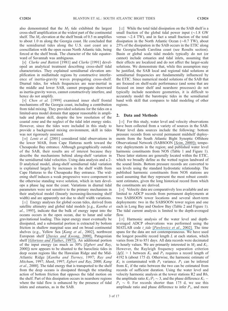
Figure 2. ADCIRC finite element model domain used for tidal computations in the northwest NorthAtlantic Ocean. The mesh contains 63,076 nodes, 111,748 elements. The 20, 35, 200, 600, 1000, 3000,and 5000-m isobaths are shown. The inset shows the grid detail in the region off of the northern coast ofGeorgia. The thick white line is a typical landward boundary for model domains that do not include theETIC along the Georgia/South Carolina coast. The 5, 10, 15, 25, and 35-m isobaths are shown. The whitesquares mark the same stations as in the inset of Figure 1.

C12024 BLANTON ET AL.: SOUTH ATLANTIC BIGHT TIDES

5 of 17

C12024

the coastal stations that are well within the sound limits(e.g., SSI, FtPl). K1 and O1 tides show comparatively littlealong-shelf variation in water level amplitudes, 0.09 m to0.11 m and 0.07 m to 0.08 m, respectively. Cross-shelfamplification is minimal.[23] Tidal ellipse parameters (semimajor/semiminor axes,

orientation, and Greenwich phase) from the velocity obser-vations are given in Table 5 for the major tidal constituentsfrom the SABSOON tower R6. The largest component isM2, with a cross-shelf velocity of 0.29 m s�1. All con-stituents rotate clockwise (the semiminor axes are all lessthan zero). For both the M2 and K1 frequencies, tidalellipses are oriented perpendicular to the isobaths withellipse eccentricities (major/minor axis length) approxi-mately w/f, where f is the Coriolis parameter and w is thetidal frequency. For semidiurnal tides, this ratio is 1.8 (at32�N) and the eccentricity is about 2.7. For diurnal tides, wis closer to f at midshelf latitudes, and the eccentricity iscloser to 1.0.[24] M2 and K1 tidal ellipse parameters for all stations

are reported in Table 6 and Figure 3. M2 major axis lengthsin the SABSOON region are 0.30 m s�1 in the midshelf(R2, R6) and decrease shoreward to 0.25 m s�1 (GR). Inthe nearshore region (LB), the ellipse becomes morerectilinear. The phase ranges from 261� to 290�, and ellipse

inclinations are oriented cross-shelf. K1 velocities are anorder of magnitude smaller than M2 and also oriented cross-shelf. The phase ranges from 100� to 135�, except at theshort-record stations GR and R5. We note that at the LBstation, the tidal ellipse rotates counterclockwise for bothfrequencies.[25] An interesting component to the water level analysis

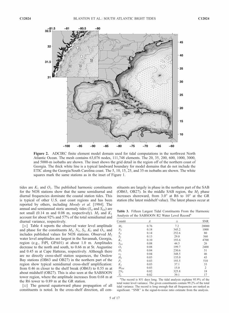
is the annual variation in the harmonic constituents. Figure 4shows amplitude and phase for M2 at Fort Pulaski, Georgia,computed from 10 years of NOS water level data. Theharmonic analysis is performed on 31-day segments andaveraged over each month. The mean M2 amplitude is about1.0 m ± 0.025 m and the mean phase is 18� ± 4�. Theamplitude variance about each month is about 0.013 m,and 2� in phase. Variation is expected in the tidal currentharmonics where seasonal stratification affects the verticalprofile of the horizontal current [e.g., Mofjeld, 1976;Prandle, 1982]. It has also been seen in water levelharmonics by Kang et al. [1995] (Yellow Sea), Foremanet al. [1995] (Victoria Sound), and Ray and Mitchum [1997](Hawaiian Ridge). This is usually attributed to seasonalstratification, which diverts barotropic tidal energy into thebaroclinic tide [Kang et al., 2002; Ray and Mitchum, 1997].The same level of variability is seen in the analysis of themidshelf SABSOON tower pressure records, but the seriesare not yet long enough for robust error estimates. We arenot aware of strong evidence of internal tides in the SAB.However, Ryan and Yoder [1996] hypothesize that observedpigment concentrations in the SAB, which were maximumalong the shelf break, could be a result of internal tides thathave been observed in coastal SAB waters [Shanks, 1988].There is also recent evidence from satellite altimetry anal-ysis of internal tides seaward of the shelf break of the SAB[Kantha and Tierney, 1997; Carrere et al., 2004]. Theextent to which these internal tides generated at the shelfbreak might affect coastal tides is not clear.[26] In the remaining sections of the paper, we will focus

on the main semidiurnal (M2) and diurnal (K1) tidal con-stituents in terms of characteristics of the observations andmodel solutions. These components represent the bulk ofthe tidal frequency variance in the SAB, and they have thelargest signal-to-noise ratio in their respective tidal speciesgroups. The characteristics of the other constituents that are

Table 4. Observed Tidal Water Level Amplitudes (m) and Phase

(�G) for Elevation Stations Listed in Table 1a

Station

M2 N2 S2 K1 O1

A f A f A f A f A f

EstuaryCHat+ 0.45 353.2 0.11 331.3 0.08 16.2 0.09 184.6 0.08 186.4BIOS 0.55 352.1 0.15 335.1 0.10 25.1 0.10 199.7 0.07 195.3BI+ 0.44 7.3 0.10 349.7 0.07 31.8 0.08 198.5 0.06 204.7Char+ 0.76 12.3 0.18 353.7 0.12 36.5 0.11 198.0 0.08 204.9CharV 0.71 357.4 0.19 346.7 0.09 36.3 0.10 190.1 0.07 196.1FtPl+ 1.03 17.9 0.23 2.1 0.16 48.4 0.11 201.0 0.08 207.3GPA01 0.95 9.5 0.26 351.5 0.16 41.2 0.13 210.9 0.08 196.5D86* 0.96 16.8 0.21 15.1 0.22 35.3 0.11 207.6 0.07 203.4SSI+ 0.97 23.8 0.21 6.1 0.15 50.8 0.11 201.3 0.08 206.4Fern+ 0.90 32.9 0.20 14.7 0.14 61.2 0.11 208.0 0.08 215.9StJ+ 0.67 26.0 0.16 5.8 0.10 50.0 0.08 203.3 0.06 211.4

ShelfOB27 0.55 353.3 0.14 335.8 0.10 17.0 0.09 184.1 0.07 189.3LB 0.73 358.6 0.15 344.0 0.12 15.0 0.12 186.8 0.07 199.5SMPier+ 0.75 357.7 0.17 337.9 0.13 18.8 0.10 189.3 0.08 193.3OB63* 0.46 352.6 0.12 320.4 0.07 27.6 0.09 201.1 0.07 188.4D87* 0.83 4.9 0.16 341.1 0.18 13.0 0.10 193.3 0.07 196.7SNLT* 0.89 6.3 0.20 2.4 0.20 19.3 0.10 195.3 0.07 194.9R6 0.68 1.5 0.17 339.7 0.13 28.0 0.10 190.9 0.07 198.0R2 0.76 7.2 0.18 345.2 0.13 29.0 0.10 193.6 0.08 199.7GR* 0.88 9.5 0.19 344.9 0.15 29.1 0.11 189.2 0.07 199.4R5* 0.76 8.0 0.17 341.7 0.13 26.8 0.11 190.2 0.07 196.3StA+ 0.66 14.3 0.16 354.8 0.11 35.7 0.10 197.0 0.07 202.4

DeepBerm 0.35 358.7 0.08 340.1 0.08 26.9 0.07 186.0 0.05 191.3Pear 0.45 357.6 0.11 335.7 0.08 23.1 0.10 190.0 0.07 194.3

aStations marked with a superscript plus are NOS water level gauges, andstations marked with a superscript asterisk have P1 infered from K1. The95% confidence intervals are as follows (except for NOS stations):Amplitude errors are less than 0.03 m. M2 phase intervals are 2� for CharVand GPA01, and less than 1� elsewhere. N2 intervals are 4�–8� for shortrecords, and 1�–2� for longer records. S2 intervals range from 1�–8�,except for CharV where it is 18�. K1 intervals range from 1�–3�. O1

intervals range from 1�–7�.

Table 5. Harmonic Analysis of the SABSOON Tower R6 Depth

Averaged Velocity Over the 913-Day Period Starting 1 April 2000a

Constit Semimajor Semiminor Inclination Phase SNR

M2 0.289 �0.105 149.2 278.5 51000N2 0.068 �0.025 149.5 258.6 2800S2 0.051 �0.019 150.7 301.4 1600K1 0.019 �0.011 136.9 107.3 350O1 0.013 �0.011 119.2 125.8 180L2 0.014 �0.004 155.3 292.0 120v2 0.013 �0.005 147.5 254.7 100P1 0.007 �0.002 148.5 97.0 46aAxes lengths are in m s�1, inclination is in degrees CCW from east, and

the phase is in degrees GMT. Sixty-eight tidal constituents were separablein the data record, which accounts for 89% and 67% of the east/west andnorth/south velocity components, respectively. The major (minor) tidalellipse axes listed account for 97% (99%) of the total tidal major (minor)axis variance. The 95% confidence intervals are ±0.001 m s�1 for all axislengths and (0.3, 1.3, 1.7, 5.5, 15.8, 5.5, 7.2, 9.5) degrees for inclination andphase, in the order listed above.

C12024 BLANTON ET AL.: SOUTH ATLANTIC BIGHT TIDES

6 of 17

C12024

close in frequency to M2 and K1 are qualitatively similar butwith reduced magnitudes.

3.2. Tidal Model Solution With ETIC

[27] The harmonic analysis of the model integration isshown in Figure 5 forM2 andK1. TheM2 amplitude (Figure 5,top) shows strong amplification on the SAB shelf, focused infront of the ETIC. Coamplitude lines are generally parallel toeach other, and range from about 0.5 m at the shelf break to1.0 m immediately in front of the ETIC. Little amplificationoccurs at the northern and southern extreme ends of the SAB.Cophase lines progress equatorward along the shelf breakand show a distinct onshelf turning at the shelf break. The

greatest phase lagat the coast, relative to that of the shelf break,occurs near the Florida/Georgia border. The cross-shelf phasedifference ranges fromabout 0� at the northern end of the SABto 18� in the middle SAB.[28] For the K1 constituent, the cross-shelf amplification

is weak. The phase progresses equatorward, also withonshelf turning at the shelf break, but without as large ofa cross-shelf phase lag seen in M2. We note that the large-scale character of the K1 tide is consistent with equatorwardpropagation as a Kelvin-like wave.[29] The model tidal velocities (Figure 5, bottom) for M2

show a substantial increase in energy shoreward of the shelfbreak, with maxima in the central midshelf region. Cross-

Table 6. M2 and K1 Ellipse Parameters From Depth-Averaged ADCP Observations and Model Solutions Sampled at Observation

Locationsa

Station

Semimajor Axis Semiminor Axis Inclination Phase

Obs Est NoEst Obs Est NoEst Obs Est NoEst Obs Est NoEst

M2

OB27 0.116 0.139 0.131 �0.058 �0.068 �0.062 119.0 139.4 137.9 261.4 255.7 261.0LB 0.071 0.071 0.064 0.014 0.012 �0.003 138.2 139.7 144.9 272.6 267.7 269.4R6 0.289 0.308 0.258 �0.105 �0.107 �0.092 149.2 154.3 156.4 278.5 275.7 267.5R2 0.312 0.330 0.271 �0.105 �0.103 �0.084 146.5 152.1 155.1 287.0 283.6 273.6GR 0.249 0.282 0.218 �0.067 �0.059 �0.037 148.5 155.3 160.6 285.6 285.0 273.7R5 0.297 0.321 0.271 �0.092 �0.103 �0.086 144.5 151.0 153.7 289.6 287.9 278.3Rms 0.022 0.028 0.007 0.018 9.7 11.2 3.6 9.8

K1

OB27 0.011 0.013 0.013 �0.007 �0.008 �0.008 70.7 104.0 102.7 132.3 108.4 114.5LB 0.009 0.005 0.005 0.003 0.002 0.001 162.4 132.8 153.5 124.0 101.1 106.0R6 0.019 0.021 0.019 �0.011 �0.012 �0.012 136.9 134.7 136.9 107.3 110.5 107.1R2 0.022 0.024 0.020 �0.010 �0.011 �0.010 121.5 132.1 134.7 115.8 118.7 114.8GR 0.020 0.018 0.015 �0.013 �0.006 �0.005 26.0 140.4 146.2 235.8 112.0 104.8R5 0.012 0.023 0.021 �0.004 �0.011 �0.011 175.1 133.4 135.8 96.4 121.3 117.2Rms - 0.003 0.002 - 0.001 0.001 - 22.9 17.9 - 16.8 12.7

aAxes lengths are in m s�1, inclination is in degrees CCW from east, and phase is in �G. The ‘‘estuary’’ (‘‘no-estuary’’) solution is given in the Est(NoEst) column. The Rms rows are the root-mean-square differences in the tidal parameters between the observations and the two model solutions. Axislength errors (in the order listed above) are ±0.001 m s�1 for long records, and ±0.003–0.007 m s�1 for shorter records (R5, GR). Phase and inclinationerrors forM2 are 0.8�, 1.6�, 0.3�, 0.9�, 1.6�, 1.5�. K1 errors are comparatively larger: 20�, 20�, 6�, 12�, 50�, 50�. The K1 rms statistics do not include the GRand R5 stations.

Figure 3. Observed versus computed (with and without estuaries)M2 and K1 tidal ellipses for the depth-averaged velocity at the ADCP stations. The inset shows the Onslow Bay and Long Bay ellipses. Thick/solid ellipses are observations, thin/solid ellipses are from the ‘‘estuary’’ solution, and dotted ellipses arefrom the ‘‘no-estuary’’ solution. The 20, 35, 200, and 600-m isobaths are shown.

C12024 BLANTON ET AL.: SOUTH ATLANTIC BIGHT TIDES

7 of 17

C12024

shelf amplitudes reach 0.30 m s�1 at the widest part of theshelf, and the phase indications (direction of flow at t = 0)are directed along-shelf poleward. K1 tidal velocities are10% of the M2 velocities, with midshelf maxima as well.Note that the K1 ellipse eccentricity is generally morecircular compared to M2. The phase indicator (flow direc-tion at t = 0) is directed along-shelf equatorward. For K1, thevelocity phase exhibits more spatial structure than that ofM2. For both frequencies, the tidal velocities rotate clock-wise except very near the coast where the rotation directionis variable and over the southern portion of the BlakePlateau.

3.3. Tidal Model Solution Without ETIC

[30] The M2 model solution without the ETIC (‘‘no-estuary’’) shows fundamental differences with the ‘‘estuary’’solution and a degradation in the agreement with the obser-vations (see section 3.4) for both tidal velocity and elevation,as given in Tables 6 and 7. This solution has substantial phaseleads and reduced elevation in the nearshore region, with thecomplex error ranging 0.05 m to 0.54 m. The midshelfstations D87, SNLT, R6, R2, GR and R5, which are seawardof the ETIC, also show increased error that results mostlyfrom a phase lead. For the shelf stations away from the ETIC(OB27, OB63, LB), there is only a small increase in theelevation error. For the tidal ellipse parameters, the rms erroris doubled (from 0.01 m s�1 to 0.02 m s�1), and the phaseerror is larger by a factor of 3.[31] In Figure 6, the M2 and K1 amplitude ratios (estuary

divided by no-estuary) and phase differences (estuary minusno-estuary) are shown for the middle SAB. The amplituderatio for M2 ranges from 1.0 (no amplification) to about 1.1

(a 10% increase in elevation) at the coast, and the phase islagged by 1� to 9�. The K1 tide does not show suchdifferences in elevation between the two solutions; thereis no amplification, and only a small 1� to 3� phase lag fromabout midshelf shoreward.[32] The presence of the estuaries increases the tidal

velocities in M2, particularly in the major axis, which isdirected shoreward. The differences in the two modelsolutions are quantified in Table 6, which reports the tidalellipse parameters for M2 and K1 at the ADCP locations forthe observations and model solutions. The M2 phase is laterin the estuary solution. Tidal velocity amplification isconcentrated in the region of the ETIC and extends pastthe midshelf. K1 shows a small increase in the major axislength but little change in the minor axis length or phase.The rms error of the axis lengths and phases for M2 issubstantially reduced in the estuary solution, as compared tothe no-estuary solution.[33] The K1 error (E in Table 7) is not as affected as M2

by removing the estuaries. For K1, the amplitude is modeledwell in both solutions, but the no-estuary solution exhibitssome large phase leads at the estuary stations. The complexerror increases for the estuary stations due more to a phaselead rather than to underpredicting the elevation. The shelfstations are not significantly affected, nor are the two deepstations. The rms statistic for K1 does not include stationsR5 and GR since the ellipse parameters are suspect.

3.4. Observations Versus Model Solutions

[34] Comparison of the model solutions (with and with-out inclusion of the ETIC) to the observed M2 and K1 waterlevels is given in Table 7. The M2 complex error E for the

Figure 4. Annual variation in the M2 amplitude (gray) and phase (white) at the NOS Fort Pulaski,Georgia, water level station. The harmonic analysis is done in 31-day segments, over 10 years of waterlevel data, and averaged over each month. Monthly means are plotted with symbols and the 95%confidence intervals are included. The NOS published values for amplitude (1.013 m) and phase (17.9�)are shown with the solid lines. The data shown are the same as in Figure 3 in Lynch et al. [2004].

C12024 BLANTON ET AL.: SOUTH ATLANTIC BIGHT TIDES

8 of 17

C12024

deep station Pear is 0.04 m (0.05 m) for the estuary (no-estuary) solution. The comparison to the no-estuary solutionis as follows: the complex error ranges from 0.03 m to0.26 m for the shelf stations, and from 0.05 m to 0.49 m forestuary stations. The estuary solution exhibits significantimprovement over the no-estuary solution. For the estuaryand shelf stations, E ranges from 0.01 m to 0.15 m and0.01 m to 0.06 m, respectively. The M2 phase is under-predicted by the no-estuary solution, particularly for theestuary stations. The amplitude and phase are shown sep-arately in Figure 7. The complex error in the estuary

solution at station BI is 0.15 m. This large error is due tothe bathymetry in the region which is not resolved wellenough. Higher resolution model solutions of the NorthCarolina coast show better skill in the ETIC in this region[Luettich et al., 1999].[35] Tidal ellipse parameters for M2 (Table 6) show good

agreement between the observations and the estuary solu-tion. There is improvement in the rms skill measure over theno-estuary solution, particularly in phase (from 9.8� to3.6�) and the minor axis lengths (from 0.017 m s�1 to0.007 m s�1).

Figure 5. (top) Computed (with ETIC) M2 and K1 elevation. Thin black lines are amplitude (m). Thickblack lines are phase (�G). For theM2 elevation amplitude and phase, the contour interval is 0.1 m and 3�.(bottom) Computed (with ETIC) M2 and K1 tidal ellipses. All ellipses rotate clockwise, except very nearthe coast and in the southwest area of the Blake Plateau. Thick black contours are the Greenwich phase,in degrees. The ticks originating at the ellipse centers are the direction of flow at t = 0 h, GMT. The 20,35, 200, 600, 1000, 3000, and 5000-m isobaths are shown with the thin grey lines.

C12024 BLANTON ET AL.: SOUTH ATLANTIC BIGHT TIDES

9 of 17

C12024

[36] For the K1 tide, E ranges from 0.00 m to 0.04 m forall stations. Tidal ellipse parameter comparisons are given inTable 6 and Figure 3. Although the K1 tidal current speedsare represented well in the model solution, there is somediscrepancy with the inclination and phase for the stationswith shorter record lengths (R5, GR). However, at the

SABSOON towers R2 and R6, the phases are within 10�of the observations.

3.5. Impact of the ETIC on Tidal Solutions in the SAB

[37] The effects of including the ETIC in the SAB aresummarized for M2 in Table 8 and Figure 7, in which the

Table 7. Modeled M2 and K1 Water Level Amplitude (m), Phase (�G), and Complex Error E (m) at the Water Level Stations

Station

M2 K1

Est NoEst Est NoEst

A f E A f E A f E A f E

EstuaryCHat 0.43 351.6 0.02 0.25 350.6 0.20 0.09 178.6 0.01 0.07 175.8 0.02BIOS 0.54 349.6 0.03 0.52 347.3 0.05 0.10 180.6 0.03 0.10 179.6 0.03BI 0.55 355.1 0.15 0.52 347.3 0.19 0.10 183.8 0.03 0.10 179.6 0.03Char 0.76 4.6 0.10 0.49 351.4 0.35 0.11 191.8 0.01 0.09 181.9 0.04CharV 0.71 353.4 0.05 0.66 351.5 0.09 0.10 186.2 0.01 0.10 185.4 0.01FtPl 0.97 16.6 0.07 0.85 358.1 0.37 0.11 198.3 0.01 0.11 189.6 0.02GPA01 0.96 9.9 0.01 0.85 358.1 0.20 0.11 194.6 0.04 0.11 189.6 0.05D86 0.98 11.2 0.10 0.53 358.7 0.49 0.11 195.4 0.02 0.08 184.7 0.04D87 0.83 3.8 0.02 0.77 358.6 0.11 0.11 190.7 0.01 0.11 189.4 0.01SSI 0.98 23.8 0.01 0.64 8.6 0.39 0.11 201.4 0.00 0.09 191.0 0.03Fern 0.89 36.9 0.06 0.41 11.0 0.54 0.11 207.9 0.00 0.08 187.9 0.04StJ 0.59 23.9 0.08 0.54 10.4 0.21 0.09 207.0 0.01 0.09 191.4 0.02

ShelfOB27 0.53 350.6 0.03 0.52 351.1 0.03 0.10 181.8 0.01 0.10 181.8 0.01LB 0.70 354.4 0.06 0.67 354.8 0.07 0.10 185.2 0.02 0.10 184.7 0.02SMPier 0.71 355.3 0.05 0.42 357.2 0.33 0.10 185.7 0.01 0.08 180.7 0.02OB63 0.44 350.2 0.02 0.44 350.2 0.03 0.10 180.7 0.01 0.10 180.7 0.01SNLT 0.91 4.8 0.03 0.83 358.0 0.14 0.11 191.6 0.01 0.11 189.4 0.01R6 0.70 0.2 0.03 0.66 356.8 0.06 0.11 188.4 0.01 0.11 187.9 0.01R2 0.78 5.0 0.04 0.74 0.3 0.09 0.11 191.1 0.01 0.11 190.0 0.01GR 0.88 9.6 0.00 0.83 3.1 0.11 0.11 193.9 0.01 0.11 192.0 0.01R5 0.76 8.1 0.00 0.74 3.3 0.07 0.11 192.6 0.01 0.11 191.7 0.00StA 0.67 12.4 0.02 0.40 10.1 0.26 0.11 195.8 0.01 0.08 190.1 0.02

DeepBerm 0.34 354.1 0.03 0.34 354.0 0.03 0.06 178.6 0.01 0.06 178.6 0.01Pear 0.41 356.2 0.04 0.40 355.8 0.05 0.09 186.1 0.01 0.09 186.0 0.01

Figure 6. M2 and K1 amplitude ratio (estuary divided by no-estuary) and phase difference (estuaryminus no-estuary) in the SAB from tidal model solutions with and without inclusion of the ETIC. Thicklines (and italics labels) are the amplitude ratio, and thin lines are the phase difference. The bathymetry isshown with the grey lines (20, 35, 200, 600, 1000, 3000, and 5000-m isobaths).

C12024 BLANTON ET AL.: SOUTH ATLANTIC BIGHT TIDES

10 of 17

C12024

elevation stations are grouped by deep, shelf and estuarystations, according to Table 1. The table gives the rmscomplex errors between the observations and the bothmodel solutions. (The estuary rms values do not includethe station BI for the reasons mentioned above.) Thereduction in elevation and phase error is evident, with thedeep water stations experiencing little change. Estuaryamplitude errors are decreased from 0.25 m to 0.03 m,and the phase errors are reduced from 13.8� to 2.8�. Shelfstation errors are reduced seven- and two-fold for amplitudeand phase, respectively. Table 8 also includes the K1 rmsstatistics. We note that this frequency is not as impacted bythe resolution of the ETIC, given the confidence intervalson the diurnal constituents. Figure 7 shows the observedand computed M2 elevation amplitude and phase. Theimprovement in phase for several stations is indicated byconnecting lines and labels.

3.6. Tidal Energetics in the SAB

[38] We examine the nature of the tidal characteristics onthe SAB shelf and in the adjacent deep ocean throughdiagnosis of the tidal energetics at the M2 and K1 frequen-cies. Generally, waves in the open ocean (removed fromreflective/dissipative boundaries) are largely progressiveand transport the tidal energy input in deep ocean regionsto shallow regions where it is dissipated through bottomfriction. Along the way, some energy is transfered to thebaroclinic tide through the interaction of the surface tidewith underlying topographic features in the presence ofstratification [Kantha and Tierney, 1997; Ray and Mitchum,1997; Munk, 1997; Egbert and Ray, 2000; Kang et al.,2000].[39] In its most basic form, the local tidal energy balance

can be written as [Egbert and Ray, 2000]:

W � � ¼ r � F ð1Þ

where W is the local work rate, � is the dissipation rate, andthe right-hand side is the divergence of the energy flux F

(equation (2)). Except in the deep ocean, where the bulk oftidal energy is input into the global oceans [Kantha, 1995],the work term is negligible and the dissipation rate is largelybalanced by the flux divergence term.[40] The energy ‘‘path’’ is indicated by the net energy

flux vector F = (Fx, Fy) over a tidal period. We diagnose thisflux from the tidal model solutions according to [Pugh,1987]:

Fx ¼1

2rghhU cos fh � fU

� �

Fy ¼1

2rghhV cos fh � fV

� �ð2Þ

where h(x, y) is the undisturbed water column depth, (h, fh)are the amplitude and phase of the computed water level,(U, fU) and (V, fV) are the amplitude and phase of thecomputed east and north velocity components, respectively.r is a reference density (1024 kg m�3) and g is gravity. Theterm cos(fh � fU,V) is the phase angle between the waterlevel and depth-averaged velocity.

Table 8. M2 and K1 rms Differences Between the Water Level

Observations and the Model Solutions, With and Without Inclusion

of the ETICa

A f E

NoEst Est NoEst Est NoEst Est

M2

Deep 0.03 0.03 3.5 3.4 0.04 0.04Shelf 0.14 0.02 4.9 2.2 0.15 0.03Estuary 0.25 0.03 13.8 2.8 0.31 0.05

K1

Deep 0.01 0.01 5.9 5.9 0.01 0.01Shelf 0.01 0.01 4.7 3.2 0.01 0.01Estuary 0.02 0.01 15.1 9.3 0.03 0.02

aThe complex error (E) and amplitude (A) are in meters, and the phase(f) is in degrees GMT. The rows are organized as Estuary, Shelf, and Deepas in Table 1. The rms statistics do not include the stations BI and BI-OS.

Figure 7. Observed versus computed M2 amplitude (m) and phase (�G). Open symbols represent the‘‘no-estuary’’ solution; solid symbols are with inclusion of the ETIC (‘‘estuary’’). The stations aregrouped into Deep (triangle), Shelf (circle), and Estuary (square). The 1:1 line is plotted, as well as the10�, �10�, and �20� error lines for the phase. The phase change for several stations is marked by thevertical lines and station labels.

C12024 BLANTON ET AL.: SOUTH ATLANTIC BIGHT TIDES

11 of 17

C12024

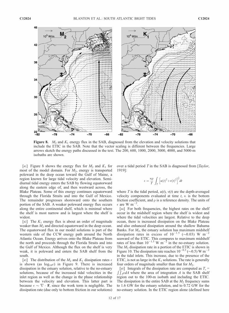
[41] Figure 8 shows the energy flux for M2 and K1 formost of the model domain. For M2, energy is transportedpoleward in the deep ocean toward the Gulf of Maine, aregion known for large tidal velocity and elevation. Semi-diurnal tidal energy enters the SAB by flowing equatorwardalong the eastern edge of, and then westward across, theBlake Plateau. Some of this energy continues equatorwardthrough the Florida Straits and into the Gulf of Mexico.The remainder progresses shoreward onto the southernportion of the SAB. A weaker poleward energy flux occursalong the entire continental shelf, which is minimal wherethe shelf is most narrow and is largest where the shelf iswidest.[42] The K1 energy flux is about an order of magnitude

weaker thanM2 and directed equatorward in the deep ocean.The equatorward flux in our model solutions is part of thewestern side of the CCW energy path around the NorthAtlantic Ocean. Energy arrives onto the Blake Plateau fromthe north and proceeds through the Florida Straits and intothe Gulf of Mexico. Although the flux on the shelf is veryweak, it is poleward and enters the SAB shelf from thesouth.[43] The distribution of the M2 and K1 dissipation rates �

is shown (as log10�) in Figure 9. There is increaseddissipation in the estuary solution, relative to the no-estuarysolutions, because of the increased tidal velocities in theinlet region as well as the change in the phase relationshipbetween the velocity and elevation. This latter part isbecause � � r � F, since the work term is negligible. Thedissipation rate (due only to bottom friction in our solutions)

over a tidal period T in the SAB is diagnosed from [Taylor,1919]:

� ¼ krT

ZT

u tð Þ2þv tð Þ2h i3

2

dt

where T is the tidal period, u(t), v(t) are the depth-averagedvelocity components evaluated at time t, k is the bottomfriction coefficient, and r is a reference density. The units of� are W m�2.[44] For both frequencies, the highest rates on the shelf

occur in the midshelf region where the shelf is widest andwhere the tidal velocities are largest. Relative to the deepocean, there is increased dissipation on the Blake Plateauand also enhanced dissipation around the shallow BahamaBanks. For M2, the estuary solution has maximum midshelfdissipation rates in excess of 10�1.5 (�0.03) W m�2

seaward of the ETIC. This compares to maximum midshelfrates of less than 10�1.5 W m�2 in the no-estuary solution.The M2 dissipation rate in a portion of the ETIC is shown inFigure 10. The dissipation rate reaches 10�0.3 (�0.5) W m�2

in the tidal inlets. This increase, due to the presence of theETIC, is not as large in the K1 solutions. The rate is generallyfour orders of magnitude smaller than that for M2.[45] Integrals of the dissipation rate are computed as T� =R RA�dA where the area of integration A is the SAB shelf

region out to the 100-m isobath and including the ETIC.The dissipation in the entire SAB at the M2 frequency sumsto 1.6 GW for the estuary solution, and to 0.72 GW for theno-estuary solution. In the ETIC region alone (defined here

Figure 8. M2 and K1 energy flux in the SAB, diagnosed from the elevation and velocity solutions thatinclude the ETIC in the SAB. Note that the vector scaling is different between the frequencies. Largearrows sketch the energy paths discussed in the text. The 200, 600, 1000, 2000, 3000, 4000, and 5000-misobaths are shown.

C12024 BLANTON ET AL.: SOUTH ATLANTIC BIGHT TIDES

12 of 17

C12024

as shoreward of the 10-m isobath), the total dissipation isabout 0.42 GW, or about 25% of the SAB dissipation. Thus,the ETIC in the SAB not only dissipates about one quarterof the energy dissipated in the SAB, but it also causes a two-fold increase in the SAB dissipation over the model solutionthat does not include the ETIC.

4. Discussion

[46] There is generally good agreement between theobservations and model solution that includes the represen-tation of the ETIC. Cross-shelf elevation amplification ofthe semidiurnal tides, particularly M2, is significant. Rela-tive to the deep ocean value of 0.45 m [Pearson, 1975], the

coastal amplification is a factor of 2.5 at the widest part ofthe shelf. Most of the amplification occurs on the continen-tal shelf, where the shelf break amplitude is uniformly0.50 m to 0.55 m. The latest M2 phase observed on theshelf proper is about 17� along the Georgia/Florida border.Previously published solutions [Chen et al., 1999] report alargest nearshore phase of 30�.[47] The K1 tidal amplitude, however, increases from the

deep value of 0.10 m to about 0.12 m. K1 tidal velocities areabout 0.01 to 0.02 m s�1, roughly the same as that reportedfor the lower MAB [Lentz et al., 2001], and smaller by afactor of 2 than K1 velocities along the west Florida shelf[He and Weisberg, 2002]. The disagreement in the K1

velocity inclination and phase at the stations R5 and GR

Figure 9. Diagnosed M2 and K1 energy dissipation per unit area (�) for tidal solutions without the ETIC(left) and with ETIC (right). The scalar shown is log10�. The total dissipation of M2 tidal energy over thetidal period in the SAB is 1.6 GW in the estuary solution and 0.72 GW in the no-estuary solution. Thetotal M2 dissipation in the ETIC is 0.42 GW, or 25% of the estuary solution dissipation in the SAB. Seecolor version of this figure at back of this issue.

C12024 BLANTON ET AL.: SOUTH ATLANTIC BIGHT TIDES

13 of 17

C12024

is large. Inference of P1 from K1 is not the source of thediscrepancy. The model solutions are smooth in this regard.We note that the O1 ellipse parameters are also variable, andthat the largest diurnal errors occur for stations with theshortest record lengths. Additionally, the diurnal tidal peri-ods are close to the inertial period in the middle SABregion, and inertial motions generated by weather-relatedforcing could be contaminating the tidal signal. Lentz et al.[2001] indicate that the K1 along-shelf velocity componentis influenced by diurnal winds on the southern MAB shelf.[48] The differences in the model solutions for M2 indi-

cate that the energy dissipated in the ETIC (in the estuarysolution) is provided by a larger-scale adjustment betweenthe water level and velocity field, relative to the no-estuarysolution. Since the M2 amplification ratio is greater than oneand the estuary solution lags the no-estuary solution on theshelf in front of the ETIC (Figure 6), this implies that highwater in the SAB is higher and occurs later in the modelsolution that resolves the ETIC.[49] Midlatitude semidiurnal tides on wide shelves expe-

rience amplification because they can propagate cross-shelfas inertia-gravity waves [Clarke and Battisti, 1981; Clarke,1991]. As the waves approach the coastal wall, they reflectand constructively interfere. Since the ETIC provides amodification to the ‘‘reflective’’ characteristics of the land-ward boundary, the reflection of semidiurnal tides issubstantially affected. Diurnal tides do not propagate asinertia-gravity waves at midlatitudes and are not as affectedby the alteration of the landward boundary region.[50] The diagnosis of this difference in solutions is shown

in Figure 11. The energy flux vector (Fx, Fy) (equation (2))is computed from both solutions, and the vector differencesare plotted. For both M2 and K1, this indicates that theremust be additional energy supplied to the estuary region,and this energy comes from offshelf, almost directly cross-

shelf. The magnitude of the K1 flux difference is about twoorders of magnitude smaller than that for M2. There is alsoan increased energy flux toward the Pamlico sound area ofthe North Carolina coast. Since the elevation on the openboundary at 60�W is identical in both solutions (andtherefore so is the elevation gradient along the boundary),the pressure work done on the open boundary is the same.However, the elevation gradient normal to the open bound-ary is not (cannot be) specified, so the velocity field at theboundary adjusts in response to the increased dissipation inthe ETIC. (The K1 difference shows a confused pattern offthe North Carolina coast. This artifact results from thedifferences in a region of rapid phase changes betweenthe two solutions.)[51] The elevation and velocity adjustments in the estu-

ary-resolving solution thus conspire to provide this addi-tional energy to the estuaries. Both the elevation andvelocity phase adjust over a large area, indicating that thecharacter of the tidal wave becomes more progressive,resulting in a larger energy flux shoreward. Tidal energyis transported toward the tidal inlet and estuary regions,where this energy is ultimately dissipated. Since the reflec-tion of the tide is not as large when the boundary isperforated with holes (which provide large energy sinks),a more progressive wave results that provides more energy.[52] The poleward M2 energy flux (Figure 8) is a branch

of the larger basin-wide poleward semidiurnal flux thattransports energy from the South Atlantic Ocean into theNorth Atlantic. According to energy budget analyses ofglobal tidal model solutions [Kantha et al., 1995; Lyard andLe Provost, 1997; Le Provost and Lyard, 1997], the NorthAtlantic Ocean dissipates more energy than is input into itthrough direct lunar and solar gravitational loading, and thusa flux of energy is required into the North Atlantic. The onlysource for this needed additional energy is flux from the

Figure 10. Diagnosed M2 energy dissipation per unit area in a part of the ETIC. The scalar shown islog10�. The 5, 10, 15, 20, and 25-m isobaths are included. See color version of this figure at back of thisissue.

C12024 BLANTON ET AL.: SOUTH ATLANTIC BIGHT TIDES

14 of 17

C12024

South Atlantic through the equatorial region (see Figure 1 inKantha et al. [1995] and Figure 2 in Lyard and Le Provost[1997]). This energy path splits in two: an eastern branchdelivers tidal energy to the northwest European shelf andArctic Ocean, and a smaller branch feeds into the Gulf ofMaine, which is seen on the eastern side of our domain.[53] The thick dashed line in Figure 8 marks the zone

along which the flux magnitude is minimum (but not zero).Locally, this implies that the wave character is morestanding (water level and depth averaged velocity in quad-rature) than progressive, or that high water occurs at nearlythe same time as minimum current speed. Although theenergy flux on the SAB shelf is poleward, the water levelphase and velocity phase are nearly in quadrature (�0� and�270�) throughout the SAB, which indicates that thesemidiurnal tides are generally standing in nature; therelative phase difference between velocity and elevation isnear, but not exactly, one quarter period. The elevation andvelocity magnitudes are also much larger on the shelf thanin deep water where the elevation and velocity are smallerbut the flux is larger (due to a smaller phase difference andlarge water column depths).[54] The North Atlantic Ocean appears to have an excess

of K1 energy input, and a flux occurs into the South Atlanticbasin (see Figure 1 in Kantha et al. [1995]). The easternside of this equatorward energy flux is seen in our solutions.On the SAB shelf, K1 has a more progressive character thandoes M2, since elevation and velocity phases are 185�–190�and 110�–130�, respectively.[55] The estuary solution exhibits an increase in M2

elevation and velocity amplitudes as well as elevation andvelocity phase adjustments, of which the energy flux anddissipation are only diagnostics. The increase in the eleva-tion amplitude in estuary solution, compared to the no-estuary solution, is contrary to the expectation that a headloss (elevation decrease) usually occurs in a more dissipa-tive environment. We are investigating this issue separately.However, the mechanism is not clear.

[56] The drag coefficient used in this study (Cd = 0.003)is slightly higher than the more typical value used invertically integrated model studies of tides (Cd = 0.0025).The higher value gives a better fit to observations through-out the entire model domain. The SAB coastal M2 waterlevels are slightly higher and earlier in a set of modelsolutions (with and without the ETIC) computed with Cd =0.0025. However, the solution without the ETIC stillexhibits a much larger overall error compared to thesolution with the ETIC. The reduced drag coefficient doesnot account for the error between the solution without theETIC and the observations. Additionally, the M2 amplifica-tion ratio and phase difference is not qualitatively affectedby the lower drag coefficient. K1 is not affected within theuncertainty of the observations.[57] The tidal energy analysis presented above focuses on

the individual tidal constituents M2 and K1. Some of the M2

energy transported onto a continental shelf is transfered intononlinear, shallow-water overtides, primarily M4 and M6.These constituents are locally generated through the inter-action of strong bathymetric gradients, nonlinear bottomfriction, and advective accelerations. In the region of thetidal inlets, these harmonics can be large and contribute tothe total energy budget for M2. We have not presented aformal energy budget for the SAB; this is the subject of afuture communication. This will include some sensitivity ofenergy dissipation and flux differences over the spring-neapcycle. The elevation range at spring tides is twice thatduring neap tides, which implies that the tidal currents arealso twice as large. The cubic nature of energy dissipationthen implies a factor of 8 difference between spring andneap dissipation rates.

5. Conclusion

[58] This study presents an analysis of tidal water leveland ADCP data in the South Atlantic Bight. Harmonicanalysis of the observations confirms previously determined

Figure 11. M2 and K1 energy flux difference between the tidal solutions with and without inclusion ofthe ETIC in the SAB. The bathymetry is shown with the light lines (20, 35, 60, 200, 1000, 3000, and5000-m isobaths).

C12024 BLANTON ET AL.: SOUTH ATLANTIC BIGHT TIDES

15 of 17

C12024

rankings of the principal tidal contributions to elevation anddepth-averaged current variability on the SAB shelf. Theseconstituents are M2, N2, S2, K1 and O1 for both water leveland currents. Additionally, we have conducted numericalsimulations using a finite element shallow-water model thatincludes a first-order representation of the estuary/tidal inletcomplex along the Georgia/South Carolina coast. It hasbeen shown that numerical solutions for the M2 tide in thenearshore, inner shelf, and midshelf zones are sensitive tothe inclusion of the ETIC. Diurnal tides are less sensitive.This substantially affects model skill for the semidiurnaltides.[59] The model solutions along the shelf break of the M2

tidal elevation amplitude and phase are consistent withbasin-scale tidal model results. Inclusion of the ETIC alongthe Georgia/South Carolina coast fundamentally modifiesthe nearshore character of computed tidal solutions anddecreases the rms error of semidiurnal tidal components forestuary and shelf stations to levels consistent with deepocean errors. We expect that further improvements will beachieved with more detailed resolution of the coastal regionas well as model solutions that include flooding anddewatering, an important process that we have notaddressed in this effort. Additional improvements may beobtained by using more recent global tidal models for theopen-water boundary conditions (e.g., the FES99 solutionsin Lefevre et al. [2002]).[60] These results demonstrate that semidiurnal tidal

solutions (particularly M2) are sensitive to the representationof complex, highly dissipative geometries. Both the cross-shelf amplification and phase lag are affected. Diurnal tidesare essentially unaffected. In light of previous tidal solutionsin the South Atlantic Bight that do not include the estuary/tidal inlet complex, it appears incorrect to compare thosesolutions with observations that either are not geometricallylocated within the domain, or in close proximity to thecoastal region.

[61] Acknowledgments. The authors thank Luke Stearns and MikeMuglia for processing the ADCP data and Karen Pehrson-Edwards forcomments on the manuscript. We also thank two anonymous reviewers,whose comments greatly improved the manuscript. We thank Jack Blantonfor providing data from stations D86, D87, and SNLT. This research wassupported under NOPP grants NAG13-00041 and N00014-98-1-0786.

ReferencesBlanton, B. O. (2003), Towards operational modeling in the South AtlanticBight, dissertation, Univ. of N. C., Chapel Hill.

Carrere, L., C. L. Provost, and F. Lyard (2004), On the statistical stability ofthe M2 barotropic and baroclinic tidal characteristics from along-trackTOPEX/Poseidon satellite altimetry analysis, J. Geophys. Res., 109,C03033, doi:10.1029/2003JC001873.

Chen, C., L. Zheng, and J. O. Blanton (1999), Physical processescontrolling the formation, evolution, and perturbation of the low-salinityfront in the inner shelf off the southeastern United States: A modelingstudy, J. Geophys. Res., 104(C1), 1259–1288.

Clarke, A. J. (1991), The dynamics of barotropic tides over the continentalshelf and slope (review), in Tidal Hydrodynamics, edited by B. Parker,pp. 79–108, John Wiley, Hoboken, N. J.

Clarke, A. J., and D. S. Battisti (1981), The effect of continental shelves ontides, Deep Sea Res., 28, 665–682.

Davies, A. M., and C. M. Kwong (2000), Tidal energy fluxes and dissipa-tion on the European continental shelf, J. Geophys. Res., 105(C9),21,969–21,989.

Egbert, G. D., and R. Ray (2000), Significant dissipation of tidal energy inthe deep ocean inferred from satellite altimeter data, Nature, 405, 775–778.

Foreman, M. G. G., and R. E. Thomson (1997), Three-dimensionalmodel simulations of tides and buoyancy currents along the west coastof Vancouver Island, J. Phys. Oceanogr., 27, 1300–1325.

Foreman, M. G. G., R. A. Walters, R. F. Henry, C. P. Keller, and A. G.Dolling (1995), A tidal model for eastern Juan de Fuca Strait and thesouthern Strait of Georgia, J. Geophys. Res., 100(C1), 721–740.

Glorioso, P., and R. Flather (1997), The Patagonian Shelf tides, Progr.Oceanogr., 40, 263–283, doi:10.1016/S0079-6611(98)00004-4.

He, R., and R. H. Weisberg (2002), Tides on the West Florida Shelf, J. Phys.Oceanogr., 32, 3455–3473.

Kang, S. K., J.-Y. Chung, S.-R. Lee, and K.-D. Yum (1995), Seasonalvariability of the M2 tide in the seas adjacent to Korea, Cont. ShelfRes., 15(9), 1087–1113.

Kang, S. K., M. G. G. Foreman, W. R. Crawford, and J. Y. Cherniawsky(2000), Numerical modeling of internal tide generation along the Hawai-ian Ridge, J. Phys. Oceanogr., 30, 1083–1098.

Kang, S. K., M. G. G. Foreman, H.-J. Lie, J.-H. Lee, J. Cherniawsky, andK.-D. Yum (2002), Two-layer tidal modeling of the Yellow and EastChina Seas with application to seasonal variability of the M2 tide,J. Geophys. Res., 107(C3), 3020, doi:10.1029/2001JC000838.

Kantha, L. H. (1995), Barotropic tides in the global ocean from a nonlineartidal model assimilating altimetric tides: 1. Model description and results,J. Geophys. Res., 100(C12), 25,283–25,308.

Kantha, L. H., and C. Tierney (1997), Global baroclinic tides, Progr.Oceanogr., 40, 163–178.

Kantha, L. H., C. Tierney, J. W. Lopez, S. D. Desai, M. E. Parke, andL. Drexler (1995), Barotropic tides in the global ocean from a nonlineartidal model assimilating altimetric tides: 2. Altimetric and geophysicalimplications, J. Geophys. Res., 100(C12), 25,309–25,317.

Lee, T. N., and D. Brooks (1979), Initial observations of current, tempera-ture, and coastal sea level response to atmospheric and Gulf Streamforcing, Geophys. Res. Lett., 6, 321–324.

Lefevre, F., F. Lyard, and C. Le Provost (2002), FES99: A global tide finiteelement solution assimilating tide gauge and altimetric information,J. Atmos. Oceanic Technol., 19, 1345–1356.

Lentz, S., M. Carr, and T. H. C. Herbers (2001), Barotropic tides on theNorth Carolina shelf, J. Phys. Oceanogr., 31, 1843–1859.

Le Provost, C., and F. H. Lyard (1997), Energetics of the M2 barotropicocean tides: An estimate of bottom friction dissipation from a hydro-dynamic model, Progr. Oceanogr., 40, 37–52.

Le Provost, C., F. H. Lyard, J.-M. Molines, M.-L. Genco, and F. Rabilloud(1998), A hydrodynamic ocean tide model improved by assimilating asatellite altimeter-derived data set, J. Geophys. Res., 103(C3), 5513–5529.

Luettich, R. A., J. J. Westerink, and N. W. Scheffner (1992), ADCIRC: Anadvanced three-dimensional circulation model for shelves, coastsand estuaries; report 1: Theory and methodology of ADCIRC-2DDIand ADCIRC-3DL, Tech. Rep. DRP-92-6, Coastal Eng. Res. Cent.,U.S. Army Eng. Waterw. Exp. Stn., Vicksburg, Miss.

Luettich, R., J. Hench, C. Fulcher, F. Werner, B. Blanton, and J. Churchill(1999), Barotropic tidal and wind driven larvae transport in the vicinity ofa barrier island inlet, J. Fish. Oceanogr., 8(2), suppl. 2, 190–209.

Lyard, F. H., and C. Le Provost (1997), Energy budget of the tidal hydro-dynamic model FES94.1, Geophys. Res. Lett., 24, 687–690.

Lynch, D. R., and C. E. Naimie (1993), The M2 tide and its residual on theouter banks of the Gulf of Maine, J. Phys. Oceanogr., 23, 2222–2253.

Lynch, D., et al. (2001), Real-time data assimilative modeling on GeorgesBank, Oceanography, 14(1), 65–77.

Lynch, D., K. Smith, B. Blanton, F. Werner, and R. Luettich (2004), Fore-casting the coastal ocean: Resolution, tide and operational data in theSouth Atlantic Bight, J. Atmos. Oceanic Technol., 21(7), 1074–1085.

Mofjeld, H. (1976), Tidal currents, in Marine Sediment Transport andEnvironmental Management, edited by D. J. Stanley and D. J. P. Swift,pp. 53–64, John Wiley, Hoboken, N. J.

Moody, J. A., B. Butman, R. C. Beardsley, W. S. Brown, D. A. Mayer, H. O.Mofjeld, B. Petrie, S. Ramp, P. Smith, and W. R. Wright (1984), Atlas oftidal elevation and current observations on the northeast American con-tinental shelf and slope, U.S. Geol. Surv., 1611.

Mukai, A., J. Westerink, R. Luettich, and D. Mark (2002), Eastcoast 2001: Atidal constituent database for the western North Atlantic, Gulf of Mexicoand Caribbean Sea, Tech. Rep. ERDC/CHL TR-02-24, Coastal andHydraul. Lab., U.S. Army Eng. Res. and Dev. Cent., Vicksburg, Miss.

Munk, W. (1997), Once again: Once again—Tidal friction, Progr.Oceanogr., 40, 7–35.

Naimie, C. E., J. W. Loder, and D. R. Lynch (1994), Seasonal variation ofthe three-dimensional residual circulation on Georges Bank, J. Geophys.Res., 99(C8), 15,967–15,989.

Pawlowicz, R., B. Beardsley, and S. Lentz (2002), Classical tidal harmonicanalysis including error estimates in MATLAB using TTIDE, Comput.Geosci., 28, 929–937.

C12024 BLANTON ET AL.: SOUTH ATLANTIC BIGHT TIDES

16 of 17

C12024

Pearson, C. (1975), Deep-sea tide observations off the southeastern UnitedStates, Tech. Rep. NOAA Tech. Memo. 17, 16 pp., Natl. Oceanic andAtmos. Admin., Rockville, Md.

Pietrafesa, L. J., J. O. Blanton, J. D. Wang, V. H. Kourafalou, T. N. Lee, andK. A. Bush (1985), The tidal regime in the South Atlantic Bights, inOceanography of the Southeastern U.S. Continental Shelf, edited by L. P.Atkinson, D. W. Menzel, and K. A. Bush, pp. 63–76, AGU, Washington,D. C.

Prandle, D. (1982), The vertical structure of tidal currents, Geophys. Astro-phys. Fluid Dyn., 22, 29–49.

Pugh, D. T. (1987), Tides, Surges, and Mean Sea Level: A Handbook forScientists and Engineers, 472 pp., John Wiley, Hoboken, N. J.

Ray, R. D., and G. T. Mitchum (1997), Surface manifestation of internaltides generated near Hawaii, Progr. Oceanogr., 40, 135–162.

Redfield, A. (1958), The influence of the continental shelf on the tides ofthe Atlantic coast of the United States, J. Mar. Res., 1492, 432–448.

Ryan, J., and J. Yoder (1996), Long-term mean and event– related pigmentdistributions during the unstratified period in South Atlantic Bight outermargin middle shelf waters, Cont. Shelf Res., 16, 1165–1183.

Seim, H. (2000), Implementation of the South Atlantic Bight SynopticOffshore Observational Network, Oceanography, 13, 18–23.

Shanks, A. (1988), Further support for the hypothesis that internal wavescan cause shoreward transport of larval invertebrates and fish, Fish. Bull.,86, 703–714.

Taylor, G. I. (1919), Tidal friction in the Irish Sea, Philos. Trans. R. Soc.London, 220, 1–93.

Tebeau, P. A., and T. N. Lee (1979), Wind induced circulation on theGeorgia shelf, Tech. Rep. 79003, 177 pp., Univ. of Miami, Miami, Fla.

Way, F. (1998), Hydrodynamic and water quality monitoring of the lowerSavannah River estuary, July to September 1997, technical report, Ga.Ports Auth., Savannah.

Werner, F. E., J. O. Blanton, D. R. Lynch, and D. K. Savidge (1993), Anumerical study of the continental shelf circulation of the U.S. SouthAtlantic Bight during the autumn of 1987, Cont. Shelf Res., 13(8/9),871–997.

�����������������������F. M. Bingham, Center for Marine Science, University of North Carolina

at Wilmington, Wilmington, NC 28409, USA.B. O. Blanton, R. A. Luettich Jr., H. E. Seim, and F. E. Werner,

Department of Marine Sciences, University of North Carolina at ChapelHill, Chapel Hill, NC 27599-3300, USA. ([email protected])D. R. Lynch and K. W. Smith, Thayer School of Engineering, Dartmouth

College, Hanover, NH 03755, USA.G. Voulgaris, Department of Geological Sciences, University of South

Carolina, Columbia, SC 29208, USA.F. Way, Applied Technology and Management, Inc., P.O. Box 20336,

Charleston, SC 29413-0336, USA.

C12024 BLANTON ET AL.: SOUTH ATLANTIC BIGHT TIDES

17 of 17

C12024

13 of 17

Figure 9. Diagnosed M2 and K1 energy dissipation per unit area (�) for tidal solutions without the ETIC(left) and with ETIC (right). The scalar shown is log10�. The total dissipation of M2 tidal energy over thetidal period in the SAB is 1.6 GW in the estuary solution and 0.72 GW in the no-estuary solution. Thetotal M2 dissipation in the ETIC is 0.42 GW, or 25% of the estuary solution dissipation in the SAB.

C12024 BLANTON ET AL.: SOUTH ATLANTIC BIGHT TIDES C12024

14 of 17

Figure 10. Diagnosed M2 energy dissipation per unit area in a part of the ETIC. The scalar shown islog10�. The 5, 10, 15, 20, and 25-m isobaths are included.

C12024 BLANTON ET AL.: SOUTH ATLANTIC BIGHT TIDES C12024