Banks' Cost of Capital and Lending∗ Anna Kovner - FDIC

Evaluating Regulatory Reform: Banks’ Cost of Capital and Lending∗

Anna Kovner† and Peter Van Tassel†

May 2019

Abstract

We examine the effects of regulatory changes on banks’ cost of capital and lending.

Since the passage of the Dodd-Frank Act, the value-weighted CAPM cost of capital

for banks has averaged 10.5% and declined by more than 4% relative to non-banks

on a within-firm basis. This decrease was much greater for larger banks subject to

new regulation than for smaller banks. Over a longer twenty-year horizon, we find

that changes in the systematic risk of bank equity have real economic consequences:

increases in banks’ cost of capital are associated with tightening in credit supply and

loan rates.

Keywords: Cost of Capital, Beta, Bank Regulation, Dodd-Frank Act, Banks

JEL Classification: G12, G21, G28

∗We are grateful to Charles Calomiris, Wilson Ervin, Stijn Van Nieuwerburgh, and Jeffrey Wurgler fordiscussing our paper and to Malcolm Baker, Mark Carey, Douglas Diamond, Fernando Duarte, VictoriaIvashina, George Pennacchi, René Stulz, and seminar participants at Chicago Booth, the Federal ReserveBank of New York’s Effects of Post-Crisis Banking Reforms Conference, the NBER Risks of Financial In-stitutions Conference, the Federal Reserve Bank of Boston, and the Columbia/BPI Conference on BankRegulation, Lending, and Growth for comments. We thank Davy Perlman, Anna Sanfilippo, and, particu-larly, Brandon Zborowski for outstanding research assistance.†Federal Reserve Bank of New York (e-mail: [email protected], [email protected]): The

views expressed in this paper are those of the authors and do not necessarily reflect the position of the FederalReserve Bank of New York or the Federal Reserve System. Any errors or omissions are the responsibility ofthe authors.

1 Introduction

Bank regulations have changed dramatically over the past twenty years. Deregulation in

the late 1990s repealed long-standing laws separating investment and commercial banking

activities, allowing for the rise of larger and more complex global banking institutions. The

financial crisis followed nearly a decade later prompting the Dodd-Frank Act (DFA) which

intensified regulation particularly for the largest banks.

In this paper, we estimate the net effect of changing regulations on banks’ cost of capital

and systematic risk, as well as the impact on bank lending supply. We find that the banking

industry’s value-weighted CAPM cost of equity capital soared to over 15% during the finan-

cial crisis, but then declined by 4.5% relative to non-banks after the passage of the DFA to

10.5%. At the same time, banks’ cost of capital has differentially increased by 1-2% in the

post-DFA period relative to the late 1990s. Time-series changes in equity betas drive these

results. Therefore, an additional interpretation of our findings is that post-crisis regulations

have lowered systematic risk in the banking industry with the cost of capital for the very

largest banks moving back toward its pre-deregulatory average. These changes matter for

the real economy – when banks’ CAPM cost of capital falls, we find that banks expand credit

supply and ease lending terms to borrowers.

Rather than focus on the impact of a single regulation, such as changes to capital stan-

dards, our approach acknowledges that banking regulations are endogenous and often change

simultaneously. For example, consider the DFA. A priori, it is unclear what effect the DFA

should have on the cost of capital for banks. The DFA increased effective capital require-

ments, established recovery and resolution frameworks, and introduced new liquidity require-

ments and leverage constraints, particularly for the largest banks. These different regulations

have varied and potentially opposing effects on the cost of capital. Safer banks may be ex-

pected to have a lower cost of capital, but any rollback in perceived government guarantees

1

may increase the cost of capital.1 Liquidity requirements may reduce the risk of bank runs

but change banks’ profitability margins.

The first contribution of this paper is to separate the net effect of regulatory changes

from other factors impacting the cost of capital such as interest rates and the business cycle.

We do this by estimating a variety of difference-in-differences specifications that compare

changes in the cost of capital for banks to non-banks across periods separated by key dates in

bank regulation. These regulatory changes are: Gramm-Leach-Bliley Act (GLB) (November

1999), Financial Crisis (January 2007), Supervisory Capital Assessment Program (SCAP)

(May 2009), and DFA (July 2010). The results highlight the importance of examining

changes to banks’ cost of capital relative to other firms and across time periods, rather than

only focusing on pre-crisis versus post-crisis changes for banks (as in Sarin and Summers

(2016)).

To confirm that we are capturing changes to bank regulation and not other factors like

interest rates, we take several approaches. First, we find similar results when we compare

banks to non-bank financial intermediaries, a control group of firms with business models

that are similar to banks but that are not directly affected by changes to bank regulation.

Second, we compare changes for banks more affected by regulation to those less affected

(large versus small). This analysis is particularly relevant when estimating changes around

the passage of the DFA. Since the DFA, we find that the CAPM cost of capital for the

largest banks has differentially declined by 3-4% relative to post-crisis highs and by 0-2%

relative to the pre-GLB period. We also look within the largest US banks and study the

staggered implementation of stress tests for banks with more than $50 billion in assets (as

1Even the impact of changes in capital requirements on the cost of equity is debated. On one hand,bankers argue that equity is more expensive than debt, so holding more equity increases the cost of capitalwith negative implications for growth and lending (see the discussion in Admati et al. (2014)). On the otherhand, academics often contend that lower leverage should lower the cost of equity capital, leaving banksindifferent to their capital structure in the absence of tax advantages for debt and other frictions (Modiglianiand Miller 1958).

2

in Flannery et al. (2017)) and find a differential decline in the CAPM cost of capital for the

very largest stress-tested banks. Overall, the results suggest that the net effect of the DFA

regulations was to lower the cost of capital for the largest banks, outweighing countervailing

effects such as the potential for lower expectations of government insurance in the post-crisis

period (Atkeson et al. 2018).

Finally, we confirm our results by repeating our main regression specifications using multi-

factor cost of capital estimates that incorporate interest rate factors (Schuermann and Stiroh

2006), CAPM cost of capital estimates with a time-varying equity risk premium (Cochrane

2011), log changes in CAPM betas that difference out the equity risk premium, and asset

betas that de-lever bank stock returns (Baker and Wurgler 2015). Across measures, we

consistently find a decrease in the cost of capital for the largest banks since the passage of

the DFA. By some measures, we also estimate that the largest banks’ cost of capital has

differentially fallen post-DFA relative to the levels that prevailed in the late 1990s.

Our approach adds a different perspective to the set of papers that study the effect of in-

dividual regulations on stock returns. For example, Baker and Wurgler (2015) show that the

low-risk anomaly holds for bank stocks with the implication that higher capital requirements

resulting in lower leverage and lower CAPM betas may not decrease the realized cost of eq-

uity capital. Gandhi and Lustig (2015) and Kelly et al. (2016) examine implied government

guarantees using size-sorted bank portfolios and equity option prices and find that too-big-

to-fail subsidies decrease the cost of capital for the largest banks and for the financial sector.

In contrast to studies that rely on a portfolio-based approach, our panel-based approach

accounts for how changing bank business models and the changing composition of regulated

banks affects the results. For example, this allows us to control for banking industry consol-

idation around the financial crisis and the increase in non-interest income over the sample

period. In addition, this paper also adds to the literature that studies how market measures

3

such as Tobin’s q are related to bank characteristics such as asset size, the value of intangi-

bles, and the composition of bank assets (Minton et al. (2017), Calomiris and Nissim (2014),

Huizinga and Laeven (2012)). For example, Calomiris and Nissim (2014) emphasize the

changing market perception of the value of bank intangibles and leverage for market-to-book

ratios. Similar to Calomiris and Nissim (2014), we find evidence of time-varying relation-

ships of some bank characteristics. Specifically, the association between risk-weighted assets

(RWA) and bank betas is strongest during the financial crisis, explaining most of the post-

financial crisis fall in the CAPM cost of capital for the banking industry in aggregate. This

result appears to be driven by loans and loan commitments, particularly real estate loans.

Even with the inclusion of time-varying controls, however, there is still a significant decline

in the post-DFA cost of capital for the largest banks, consistent with the interpretation that

regulation has lowered systematic risk.

The final contribution of the paper is to document that these changes in banks’ CAPM

cost of capital matter for the real economy, thus relating our analysis to the real effects of

bank regulation. We hypothesize that banks’ CAPM cost of capital matters because the

CAPM is used in practice by managers, investors, and lawyers (Graham and Harvey (2001),

Berk and van Binsbergen (2016), Gilson et al. (2000)). For example, for non-financial firms,

investment is sensitive to the cost of debt and the weighted average cost of capital (Philippon

(2009), Gilchrist et al. (2013), Frank and Shen (2016)). Bank managers anecdotally use cost

of capital estimates to allocate capital across divisions and bank CEOs cite the need to meet

investors’ return on equity targets as documented in annual reports and in bank executive

compensation packages (Pennacchi and Santos 2018). To our knowledge, this study is the

first to establish an empirical relationship between bank-level CAPM cost of capital estimates

and bank lending supply.

We establish this link using confidential bank level survey response data from the Senior

4

Loan Officer Opinion Survey (SLOOS), a survey used to measure banks’ willingness to lend

that allows us to separate credit supply effects from demand (Lown and Morgan (2006),

Hirtle (2009), Bassett et al. (2014), DeYoung et al. (2015)). We find that changes in the

cost of capital are associated with changes in the supply and the pricing of credit. This

result holds in aggregate for the panel of surveyed banks as well as in the cross section

after controlling for changes in the risk-free rate, business cycle variation, and bank-level

stock market returns to account for firm-specific shocks. When banks’ CAPM cost of capital

increases, bank managers tighten loan standards and increase loan spreads. Through this

channel, regulations that lower CAPM costs of capital after DFA are passed through to the

real economy.

2 Estimating the cost of capital

2.1 CAPM cost of capital

The cost of capital reflects the expected return of equity investors as well as the time value of

money as captured by the risk-free rate. Empirically, expected stock returns are not observed.

Instead, we must rely on economic or statistical models to estimate expected returns. As

a result, any test regarding the cost of capital is a joint test of the null hypothesis and the

model that is used to estimate expected returns (Fama 1970). We use the CAPM for our

baseline cost of capital analysis, but confirm our results are robust to other measures in

Section 6. Our focus on the CAPM is motivated by its widespread use in practice. The

relevance of this approach is evident in section 5 where we find the CAPM cost of capital

affects bank lending supply

5

We define our estimate of the CAPM cost of capital as,

CAPMi,t = Rft + βi,t · µ. (1)

The first term is the risk-free rate Rft. The second term is a time-varying CAPM beta

βi,t. The last term is the equity risk premium µ, which we assume is constant.2 We set

the risk-free rate to the three-month Treasury bill rate and the equity risk premium to 8%,

the average CRSP value-weighted excess return from 1926 to 2017. The betas are estimated

from one-year rolling regressions of firm-level daily excess returns onto market excess returns.

The market return is the CRSP value-weighted return obtained from Ken French’s website.

The estimates are ex-ante betas in the sense that each month the beta is computed using

lagged daily data over the previous 252 trading days.

A number of alternative choices can be made when estimating betas. For example, to

name a few methods from a large literature, betas can be estimated from five-year rolling

regressions with monthly data, one-year rolling regressions with daily data, or directly from

volatility and correlation estimates.3 Betas may also use lagged, centered, or forward data

depending on the application. Given our interest in how the cost of capital has varied

over time, we prefer using daily data (252 observations per year) to deliver more precise

and less biased estimates in comparison to slow moving estimates from monthly data (60

observations per five years). We use an ex-ante (lagged) approach in order to approximate

2Betas can be estimated precisely with high frequency data. In contrast, the equity risk premium isnotoriously difficult to estimate. Even with a constant risk premium and log-normal returns, it would takeover forty years to estimate the equity risk premium with a standard error of 3% (Merton 1980). Thisimprecision dominates the uncertainty in estimating expected returns in factor model settings (Fama andFrench 1997). Empirically, Welch and Goyal (2007) find that many models under perform the historicalmean and are unstable out of sample. Based on this observation and for simplicity, we assume the equityrisk premium is a constant equal to the historical mean in our baseline analysis. We relax this assumptionin Section 6.

3For example, see Scholes and Williams (1977), Fama and French (1997), Ang and Kristensen (2012),Frazzini and Pedersen (2014), and Baker and Wurgler (2015).

6

manager estimates of their cost of capital.

An implication of this approach is that we rely on the time-series and cross-sectional

differences in betas to identify changes in the cost of capital. If we assume the CAPM

holds and the equity risk premium is roughly constant over our regulatory periods, time

variation in betas will reflect how the cost of capital is changing for banks relative to other

firms, even if there is large uncertainty surrounding the level of the cost of capital itself.

Of course, the well-documented low-risk anomaly and time-variation in discount rates pose

challenges for this interpretation (Black et al. (1972), Cochrane (2011), Frazzini and Pedersen

(2014), Baker and Wurgler (2015)). Stocks with high (low) equity betas have historically

earned lower (higher) returns than predicted by the CAPM and variation in price-dividend

ratios indicate that either discount rates or cash flow growth rates are varying over time.

To account for this, Section 6 explores the robustness of our results to alternative cost of

capital estimates including multi-factor models, the CAPM with a time-varying equity risk

premium, and the weighted average cost of capital (WACC).4

2.2 Sample selection and definition of banks

We use CRSP, Compustat, and regulatory data from call reports and Y-9C filings from

March 1996 to December 2017 when estimating the cost of capital and for panel regressions

with bank characteristics. We estimate the cost of capital for all CRSP firms with share

codes 10 or 11 that are traded on the NYSE, NASDAQ, or AMEX. Later in the paper we

also estimate asset betas by merging quarterly Compustat data onto monthly CRSP data

using the most recent observation that was announced prior to the start of the month (based

on RDQ date). We filter observations from this dataset with missing cost of capital estimates

4In comparison to the CAPM, multi-factor models have been criticized for poor out-of-sample perfor-mance and for data snooping (Linnainmaa and Roberts (2016), Harvey et al. (2016)) . Larger models alsohave the disadvantage that they are less likely to be used by managers.

7

or missing Compustat asset data as well as observations with share prices that are less than

one dollar. The resulting sample includes a panel of 1,111,127 firm-month observations.5

Defining banks within this sample is not straightforward. Limiting banks to depository

institutions in SIC code 60 would exclude firms that became bank holding companies after

the financial crisis in 2009. These firms are subject to financial regulation that is a key object

of interest in this analysis. We therefore expand our definition to include both firms that

are depository institutions (SIC code 6020-6036) as well as firms that have an RSSDID (the

unique identifier assigned to financial institutions by the Federal Reserve) between the first

and the last dates when regulatory assets from Y-9C filings are within 10% of total assets

from Compustat. Firms that fulfill either of these criteria in month-t are identified as banks

by the binary variable Banki,t. We identify RSSDIDs using the FRBNY RSSDID-Permco

crosswalk, which matches banks between Compustat and regulatory reports using name,

city and state, and financial variables.6 Of the 11,961 firms in the sample, 1,415 firms are

identified as banks throughout the sample while 34 firms are identified as banks for only

part of the sample, including Metlife, Goldman Sachs, and Morgan Stanley. Because we

include savings and loans in our definition as banks, and these firms only file call reports

after 2012:Q1, there are fewer banks with regulatory data than there are total banks. The

result is a sample containing 99,049 bank-month observations for banks with regulatory data

5In the event that firms issue multiple securities, we obtain unique firm-month observations by retainingthe PERMCO-date pairs for the security (PERMNO) that has the largest market capitalization each month.Our use of the most recent quarterly accounting data from Compustat is similar to Hou et al. (2014) andAdrian et al. (2015) who form portfolios based on recent quarterly earnings data. This differs from Famaand French (1993) who form portfolios annually.

6SIC codes are obtained with descending priority from Compustat historical, Compustat header, CRSPhistorical, or CRSP header data depending on availability following the procedure described in Adrian et al.(2015). RSSDID-Permco matches are based on the FRBNY crosswalk as of 2016q4. This definition of banksdiffers from an entirely SIC code or NAICS driven approach. For example, 24 companies with SIC code 6099(functions related to depository banking) are not coded as banks at some point in our sample. This subsetincludes some of the credit card companies that do not have an RSSDID or regulatory assets that matchCompustat data (i.e. Mastercard, Visa). At the same time, 13 companies with an SIC code beginning with62 are coded as banks in our analysis (i.e. Goldman Sachs, Morgan Stanley). We exclude AIG from thesample.

8

when all regulatory variables are available as compared to 142,189 bank-month observations

for the cost of capital.

3 Measuring changes over time in the cost of capital

We compare changes in the cost of capital across time periods in which bank regulations

changed from 1996 to 2017. The periods are:

1. Basel I: Pre-period (March 1996 to October 1999)

2. GLB: The Gramm-Leach-Bliley Act (November 1999 to December 2006)

3. Crisis: The Financial Crisis (January 2007 to April 2009)

4. SCAP: The Supervisory Capital Assessment Program (May 2009 to June 2010)

5. Dodd-Frank: The Dodd-Frank Act (July 2010 to December 2017)

We define break points as the month of the passage of the relevant banking law. Results

are similar if we vary the time periods within a few months to capture anticipation of the

passage of the law. Figure 1 plots the monthly value-weighted average cost of capital for

banks with dashed-horizontal lines at the means of the different regulatory time periods.

These simple averages do not control for differences in the composition of the panel nor

firm characteristics, and confidence intervals around these means would not account for the

the fact that the observations are not independent (neither over time nor within firm). We

therefore estimate the following specification to see how the cost of capital has changed over

time:

CAPMi,t = α+ β1GLBt + β2Crisist + β3SCAPt + β4Dodd-Frankt + ei,t (2)

where CAPMi,t is the estimated CAPM cost of capital and GLBt, Crisist, SCAPt, and

Dodd-Frankt are binary variables equal to one during the periods defined above. The

9

omitted pre-period begins twenty years ago in 1996 and thus is characterized by the Basel I

regulatory regime.

The estimated coefficient for each time period is the difference between the average cost of

capital in that time period relative to the pre-period, whose value is captured by the constant

term. The null hypothesis is that all β are equal to 0 – meaning that there have not been any

changes to the CAPM cost of capital over time and, as a result, that regulatory changes have

not changed the cost of capital. We estimate the specifications both on a value-weighted

and equal-weighted basis to understand how the cost of capital is changing in aggregate and

for the average company in the panel. Standard errors are clustered by firm and by month.

Results are similar if the analysis incorporates earlier data (back through 1986), however,

we focus on the more recent time period to have consistency in the regulatory data, which

becomes available for all fields used in the analysis starting in 1996:Q1.

3.1 Difference-in-differences across industries

We estimate our first difference-in-differences regressions by adding a bank indicator variable

that is interacted with each of the time period dummies,

CAPMi,t −Rft = α+ β1GLBt + β2Crisist + β3SCAPt + β4Dodd-Frankt

+ρBanki,t + δ1Banki,t ·GLBt + δ2Banki,t · Crisist + δ3Banki,t · SCAPt

+δ4Banki,t ·Dodd-Frankt + ei,t

(3)

This specification nets out the risk-free rate Rft and allows the cost of capital to change

differently for banks and non-banks around the time periods when bank regulation changed.

When we estimate δ that are different from 0, changes to the cost of capital for banks relative

to the pre-period are different from that for non-banks.

This approach allows us to mitigate issues with the changing composition of the panel

10

over time by estimating the same regression absorbing firm fixed effects αi that replace

the constant α. The changing panel would otherwise present an issue around the financial

crisis as a number of very large banks and broker dealers exit the sample due to mergers or

bankruptcy while a number of very large broker dealers and credit card companies become

bank holding companies. Beyond the crisis, there are also changes in the panel throughout

the sample due to private firms entering by going public and public firms exiting as a result

of mergers and acquisitions. In addition to the changing panel, we also begin to control for

firm characteristics by narrowing in on the effect of changing leverage. Some specifications

include controls for Leveragei,t which is defined as total debt divided by the market value

of assets (total debt plus the market value of equity). For banks we add total deposits

to total debt when calculating leverage because the Compustat measure of total debt does

not include deposits. In unreported regressions, we include 3-digit SIC code fixed effects as

controls and expand the the definition of banks to include all firms that have RSSDIDs, and

results are similar.

3.2 Top firms

While the difference-in-differences regressions highlight the change in the cost of capital for

banks relative to other firms, they potentially conflate the impact of changing regulation

with other sources of time variation in the cost of capital. The cost of capital for the very

largest firms in any industry may be different from that of smaller firms, for example, as a

result of differences in systematic risk, market beliefs about implicit government support, or

an association between firm size and market power.7 In the bond market, Hale and Santos

(2014) find that all large firms pay lower rates for bonds, and the very largest banks pay

7While large banks may be better diversified, diversification may not result in reduced risk to the extentthat it facilitates greater leverage or riskier lending (Demsetz and Strahan 1997). As a result, large anddiversified banks may still be exposed to the economy in general, resulting in high systematic risk which isthe only risk priced in the CAPM.

11

differentially lower rates than non-banks. Further, the relationship between size and expected

returns can change over time. To better understand the impact of regulation targeted at the

largest banks, we thus need to ensure that we difference out changes over time in the cost

of capital by size so we do not attribute those changes to changes in bank regulation.

To build a time series of large banks, we look more closely at the subset of banks most

affected by post financial crisis regulatory changes, banks with more than $50 billion in assets.

Banks with more than $50 billion in assets are approximately the twenty largest banks in

the US, so we create a dummy variable (“Top”) to capture the largest twenty firms by total

assets within each industry at each point in time. We define industries by SIC code using the

twelve industry portfolios on Ken French’s website and split financials into banks and non-

bank financials using the definition described before. This gives us a measure that we can use

over a long time series and across industries. We repeat the analysis from equation 3 adding

interactions between our coefficients of interest and the Top dummy variable. A significant

interaction between Top, time period, and bank indicates that the difference between Top

banks and smaller banks is different than the difference between Top non-banks and non-Top

non-banks in the current period relative to the pre-period.

3.3 The role of bank characteristics

In order to understand how changes to bank business models, capital, and liquidity are

affecting their cost of capital, we zoom in on regulated banks for which we have detailed

income statement and balance sheet data (call reports and Y-9C filings). We estimate the

12

following regression:

CAPMi,t −Rft = α+ β1GLBt + β2Crisist + β3SCAPt + β4Dodd-Frankt

+ρBanki,t + δ1Banki,t ·GLBt + δ2Banki,t · Crisist + δ3Banki,t · SCAPt

+δ4Banki,t ·Dodd-Frankt + θ ·Xi,t + φ1 ·Xi,t ·GLBt + φ2 ·Xi,t · Crisist

+φ3 ·Xi,t · SCAPt + φ4 ·Xi,t ·Dodd-Frankt + ei,t.

(4)

We continue to include the full panel of companies and add dummy variables for missing

regulatory data (omitted in the equation above). To proxy for capital and liquidity, we

include in X the proportion of total liabilities funded with core deposits, the Tier 1 capital

ratio, and a proxy for the liquidity coverage ratio (weighted assets divided by weighted

liabilities including off balance sheet commitments x 100)8. For asset composition and risk

we include the proportion of non-interest income to total income and the ratio of risk-

weighted assets to total assets. We also include specifications that decompose risk-weighted

assets into its components including the proportion of cash-equivalent assets, loans, trading

assets, commitments, and derivatives to total assets. All balance sheet items are measured

as of the most recent quarter. Table 1 presents summary statistics for these variables in

Panel A over the full sample period. Panel B tabulates the value-weighted averages for each

regulatory regime, illustrating how the asset composition, funding mix and asset risk of the

banking industry have changed over time.

Changes in regulation can impact banks’ cost of capital by changing bank risk, capital,

liquidity, and business models. At the same time, bank managers may change their firm’s

characteristics in response to time-varying investment opportunities or in response to changes

in the market’s evaluation of bank risks, thereby impacting their cost of capital. We decom-

8LCR proxy uses regulatory data to approximate the LCR ratio as follows: Assets are weighted andinclude: Cash, FF Repo, US treasury, Agency Securities, Municipal securities, MBS, Other securities, Loans.Liabilities include respective weights times the following: FF Repo, Trading Liabilities, Commercial Paper,OBM, Subdebt, Deposits. Off balance sheet securities include respective weights times the following: Unusedcommitments, Financial Standby Letters, Securities underwritten, Securities lent.

13

pose this by first studying the impact of controlling for bank characteristics unconditionally

(φ = 0). We then interact the bank characteristics with the time period dummy variables

to allow the coefficients to change over time (φ 6= 0). This allows us to understand whether

changes to expected returns arise from changes to the market price of risk for different char-

acteristics both within and across firms. For example, if liquidity has a large and significant

coefficient only in the SCAP time period, this will be reflected in the φ3 coefficient, absorbing

variation that would have been reflected in the SCAP time period dummy in regression spec-

ification 4. The Appendix extends this analysis to the difference-in-differences regressions

for the Top banks.

3.4 Effect of stress testing

We also look in detail at the effect of stress testing on the cost of capital by adopting the

identification approach of Flannery et al. (2017) to estimate how stress tests impact the cost

of capital:

CAPMi,t −Rft = α+ β1GLBt + β2Crisist + β3SCAPt + β4Pre-CCARt+

β5Post-CCARt + β6SCAP Firmi + β7CCAR Firmi + β8SCAP Firmi · SCAPt

+β9SCAP Firmi · Pre-CCARt + β10SCAP Firmi · Post-CCARt

+β11CCAR Firmi · Post-CCARt + θ ·Xi,t + ei,t.

(5)

Each specification includes a set of non-overlapping time fixed effects and controls for bank

characteristics X. We split the banks into two groups based on the timing of their exposure

to Federal Reserve stress testing. The first banks exposed to stress testing are captured

by the binary variable SCAP Firmi which is equal to 1 for the largest BHCs that were

initially included in stress tests beginning with SCAP in 2009.9 The next banks exposed

9Two US stress tested firms were not public for the entire sample. The first observation for Ally (SCAP)is April 2015 and the first observation for Citizens (CCAR) is September 2015.

14

to stress testing are captured by the binary variable CCAR Firmi which is equal to 1 for

the banks subjected to Comprehensive Capital Analysis and Review (CCAR) stress tests

starting in 2014 (“CCAR 2014 Addition”). The regulatory time periods are also changed to

accommodate the phased implementation of stress testing by splitting the DFA period into

two sub-periods before and after the expansion of firms subject to stress testing:

1. Pre-CCARt: Passage of the Dodd-Frank Act when the 18 firms (SCAP Firmi) are

subject to stress testing and associated disclosure (July 2010 to August 2013)

2. Post-CCARt: Addition of 7 firms (CCAR Firmi) to stress testing and associated

disclosure (September 2013 to December 2017)

As in Flannery et al. (2017), we limit the panel to the top 90 banks by assets each month

to ensure that our comparison group of non-stress-tested banks is closer to the group of

stress-tested banks.

3.5 Effects on credit supply

We are interested in understanding if changes in the cost of capital for banks have effects

on the real economy through the provision and pricing of credit. For this, we make use of

the Senior Loan Officer Opinion Survey (SLOOS), which provides qualitative and limited

quantitative information on the standards and terms of bank lending, business conditions,

and household demand for loans as measured by survey responses of senior loan officers.

We make use of the SLOOS data because it offers a way to separate changes to lending

standards from changes in demand. This approach is superior to a simple estimation of the

relationship between loan balances and interest margins using bank holding company data,

because those measures conflate the supply of bank lending with demand.10 The Federal10We do not estimate a statistically significant relationship between quarterly changes in loan balances

or interest margins and banks’ cost of capital.

15

Reserve conducts the SLOOS at a quarterly frequency covering questions about changes in

the supply and demand for loans over the previous three months as well as special topics on

evolving developments and lending practices in U.S. loan markets. As of 2017, the panel of

reporting banks in the SLOOS included up to eighty large domestically chartered commercial

banks that span all Federal Reserve Districts and up to 24 large U.S. branches and agencies

of foreign banks that are primarily located in the New York District.

Our analysis focuses on questions that cover changes in lending standards and loan terms

relative to the previous quarter. Using survey responses instead of measuring balance sheet

loan growth or changes in interest income allows us to focus on the supply effect at the

individual bank level. We make use of survey questions on credit standards such as this

example from the July 2018 SLOOS:

Over the past three months, how have your bank’s credit standards for approving appli-

cations for C&I loans or credit lines—other than those to be used to finance mergers

and acquisitions—to large and middle-market firms and to small firms changed?

Possible survey responses included: eased considerably, eased somewhat, remained basically

unchanged, tightened somewhat, and tightened considerably. The questions are collected

for loan standards to both large and middle-market firms (annual sales of $50 million or

more) as well as small firms. Consistent with previous work using this data, we code these

categorical responses as variables equal to -2, -1, 0, 1, and 2 in our regression analysis,

with higher numbers indicating a tightening of credit standards or a tightening of the terms

for loans that banks are willing to approve including the cost of credit lines, the spread of

loan rates over bank’s cost of funds, the premium charged on riskier loans, loan covenants,

collateralization requirements, and the maximum size of credit lines.

The regression specification for this analysis is:

16

SLOOSi,t = α+ η ·∆(CAPMi,t −Rft) + ei,t. (6)

We regress bank-level SLOOS survey responses, a quarterly change, onto one-year changes

in bank-level CAPM cost of capital estimates net of the risk-free rate. Similar results hold

using six-month and two-year changes in the cost of capital and when we lag the change in

the cost of capital by a quarter relative to the survey response. In addition, we also report

specifications that control for one-year changes in the risk-free rate and one-year lagged

realized bank-level stock market returns. This helps to confirm that we are identifying a

relationship between the CAPM cost of capital and lending supply and that the results are

not explained by omitted variables like bank distress. Finally, we add time fixed effects to

absorb business cycle variation in the survey responses. A positive coefficient on η in these

regressions indicates that bank managers are tightening credit standards or loan terms when

their cost of capital is increasing.

4 The impact of regulation on the cost of capital

Over the last twenty years, value-weighted expected returns for banks averaged 11.5% based

on an unbalanced panel of 1,447 banks. This compares to expected returns for non-banks of

10.0% (value weighted, based on an unbalanced panel of 10,545 non-banks). The risk-free

rate averaged 2.2% over our sample period, and as mentioned in Section 2, we set the level

of the equity risk premium to 8% for our baseline cost of capital estimates. In comparison

to these averages, Table 2 presents the results from estimating equation 2 on different panels

of firms. Dependent variables include the CAPM cost of capital and risk premium (CAPM

and CAPM-Rf), the Fama and French (1993) three-factor risk premium (FF3-Rf), and the

monthly realized excess return multiplied by twelve (Realized-Rf). Regressions are estimated

17

on an equal-weighted (EW) basis as well as a value-weighted (VW) basis.11 The average

level of the estimated cost of capital in any time period can be calculated by summing

the coefficient for the time period with the constant, which captures the average (EW) or

weighted average (VW) for the pre-GLB period.

4.1 Difference-in-differences across industries

In order to see if changes in the cost of capital for banks are different from those of non-banks

over time, Table 3 combines all firms into a single panel and estimates the specification in

equation (3) for the CAPM cost of capital and risk premium. The decline of more than 4

percentage points in the risk free rate since the late 1990s is reflected in column (1).

In the remaining columns we explore differences between banks and nonbanks. We esti-

mate that banks’ value-weighted cost of capital is about 70 basis points higher than that of

other firms on average, consistent with the higher systematic risk of banks as evidenced by

their average value-weighted beta of 1.17. But this premium has changed over time relative

to the pre-GLB period. In the GLB period, the cost of capital for banks is unusually low rel-

ative to non-banks (Bank x GLB coefficient of -1.25). This result is surprising because most

interpret GLB as being deregulatory and therefore related to an increase in the systemic risk

of banks. In the Dodd-Frank period, the cost of capital for banks is 3% lower overall but

1.90% higher relative to non-banks (Dodd-Frank coefficient of -4.91 + Bank x Dodd-Frank

coefficient of 1.90). Changes in banks’ cost of capital diverge the most from non-banks in

the period immediately following the financial crisis and prior to the passage of the DFA –

comparing the current period to the SCAP period, banks’ cost of capital fell by approxi-

mately 4.5% (Bank x SCAP coefficient of 6.55 minus Bank x Dodd-Frank coefficient of 1.90),

while the change in the cost of capital in those time periods for non-banks was roughly zero11The value weights are proportional to lagged market capitalization and are normalized each month by

the total lagged market capitalization of all firms in the panel.

18

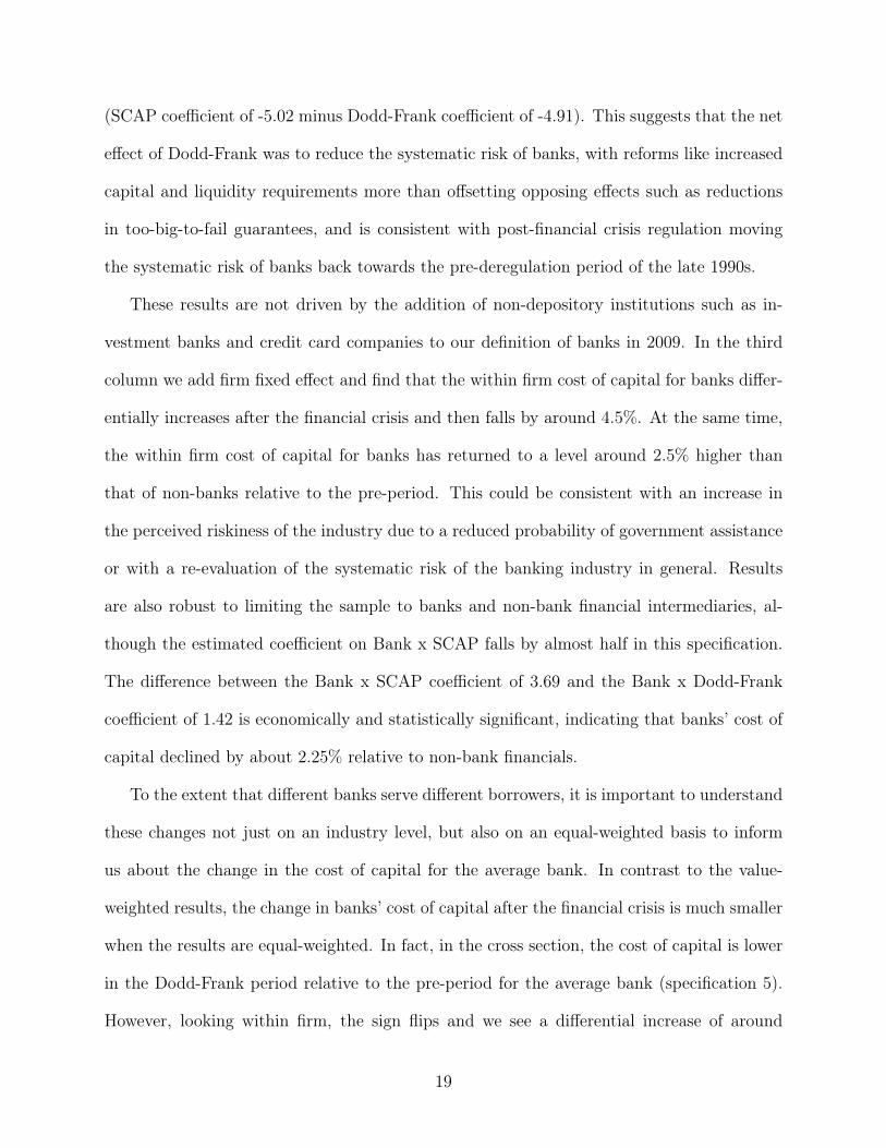
(SCAP coefficient of -5.02 minus Dodd-Frank coefficient of -4.91). This suggests that the net

effect of Dodd-Frank was to reduce the systematic risk of banks, with reforms like increased

capital and liquidity requirements more than offsetting opposing effects such as reductions

in too-big-to-fail guarantees, and is consistent with post-financial crisis regulation moving

the systematic risk of banks back towards the pre-deregulation period of the late 1990s.

These results are not driven by the addition of non-depository institutions such as in-

vestment banks and credit card companies to our definition of banks in 2009. In the third

column we add firm fixed effect and find that the within firm cost of capital for banks differ-

entially increases after the financial crisis and then falls by around 4.5%. At the same time,

the within firm cost of capital for banks has returned to a level around 2.5% higher than

that of non-banks relative to the pre-period. This could be consistent with an increase in

the perceived riskiness of the industry due to a reduced probability of government assistance

or with a re-evaluation of the systematic risk of the banking industry in general. Results

are also robust to limiting the sample to banks and non-bank financial intermediaries, al-

though the estimated coefficient on Bank x SCAP falls by almost half in this specification.

The difference between the Bank x SCAP coefficient of 3.69 and the Bank x Dodd-Frank

coefficient of 1.42 is economically and statistically significant, indicating that banks’ cost of

capital declined by about 2.25% relative to non-bank financials.

To the extent that different banks serve different borrowers, it is important to understand

these changes not just on an industry level, but also on an equal-weighted basis to inform

us about the change in the cost of capital for the average bank. In contrast to the value-

weighted results, the change in banks’ cost of capital after the financial crisis is much smaller

when the results are equal-weighted. In fact, in the cross section, the cost of capital is lower

in the Dodd-Frank period relative to the pre-period for the average bank (specification 5).

However, looking within firm, the sign flips and we see a differential increase of around

19

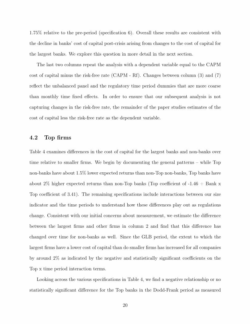
1.75% relative to the pre-period (specification 6). Overall these results are consistent with

the decline in banks’ cost of capital post-crisis arising from changes to the cost of capital for

the largest banks. We explore this question in more detail in the next section.

The last two columns repeat the analysis with a dependent variable equal to the CAPM

cost of capital minus the risk-free rate (CAPM - Rf). Changes between column (3) and (7)

reflect the unbalanced panel and the regulatory time period dummies that are more coarse

than monthly time fixed effects. In order to ensure that our subsequent analysis is not

capturing changes in the risk-free rate, the remainder of the paper studies estimates of the

cost of capital less the risk-free rate as the dependent variable.

4.2 Top firms

Table 4 examines differences in the cost of capital for the largest banks and non-banks over

time relative to smaller firms. We begin by documenting the general patterns – while Top

non-banks have about 1.5% lower expected returns than non-Top non-banks, Top banks have

about 2% higher expected returns than non-Top banks (Top coefficient of -1.46 + Bank x

Top coefficient of 3.41). The remaining specifications include interactions between our size

indicator and the time periods to understand how these differences play out as regulations

change. Consistent with our initial concerns about measurement, we estimate the difference

between the largest firms and other firms in column 2 and find that this difference has

changed over time for non-banks as well. Since the GLB period, the extent to which the

largest firms have a lower cost of capital than do smaller firms has increased for all companies

by around 2% as indicated by the negative and statistically significant coefficients on the

Top x time period interaction terms.

Looking across the various specifications in Table 4, we find a negative relationship or no

statistically significant difference for the Top banks in the Dodd-Frank period as measured

20

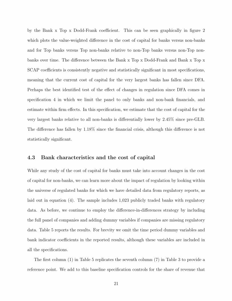
by the Bank x Top x Dodd-Frank coefficient. This can be seen graphically in figure 2

which plots the value-weighted difference in the cost of capital for banks versus non-banks

and for Top banks versus Top non-banks relative to non-Top banks versus non-Top non-

banks over time. The difference between the Bank x Top x Dodd-Frank and Bank x Top x

SCAP coefficients is consistently negative and statistically significant in most specifications,

meaning that the current cost of capital for the very largest banks has fallen since DFA.

Perhaps the best identified test of the effect of changes in regulation since DFA comes in

specification 4 in which we limit the panel to only banks and non-bank financials, and

estimate within firm effects. In this specification, we estimate that the cost of capital for the

very largest banks relative to all non-banks is differentially lower by 2.45% since pre-GLB.

The difference has fallen by 1.18% since the financial crisis, although this difference is not

statistically significant.

4.3 Bank characteristics and the cost of capital

While any study of the cost of capital for banks must take into account changes in the cost

of capital for non-banks, we can learn more about the impact of regulation by looking within

the universe of regulated banks for which we have detailed data from regulatory reports, as

laid out in equation (4). The sample includes 1,023 publicly traded banks with regulatory

data. As before, we continue to employ the difference-in-differences strategy by including

the full panel of companies and adding dummy variables if companies are missing regulatory

data. Table 5 reports the results. For brevity we omit the time period dummy variables and

bank indicator coefficients in the reported results, although these variables are included in

all the specifications.

The first column (1) in Table 5 replicates the seventh column (7) in Table 3 to provide a

reference point. We add to this baseline specification controls for the share of revenue that

21

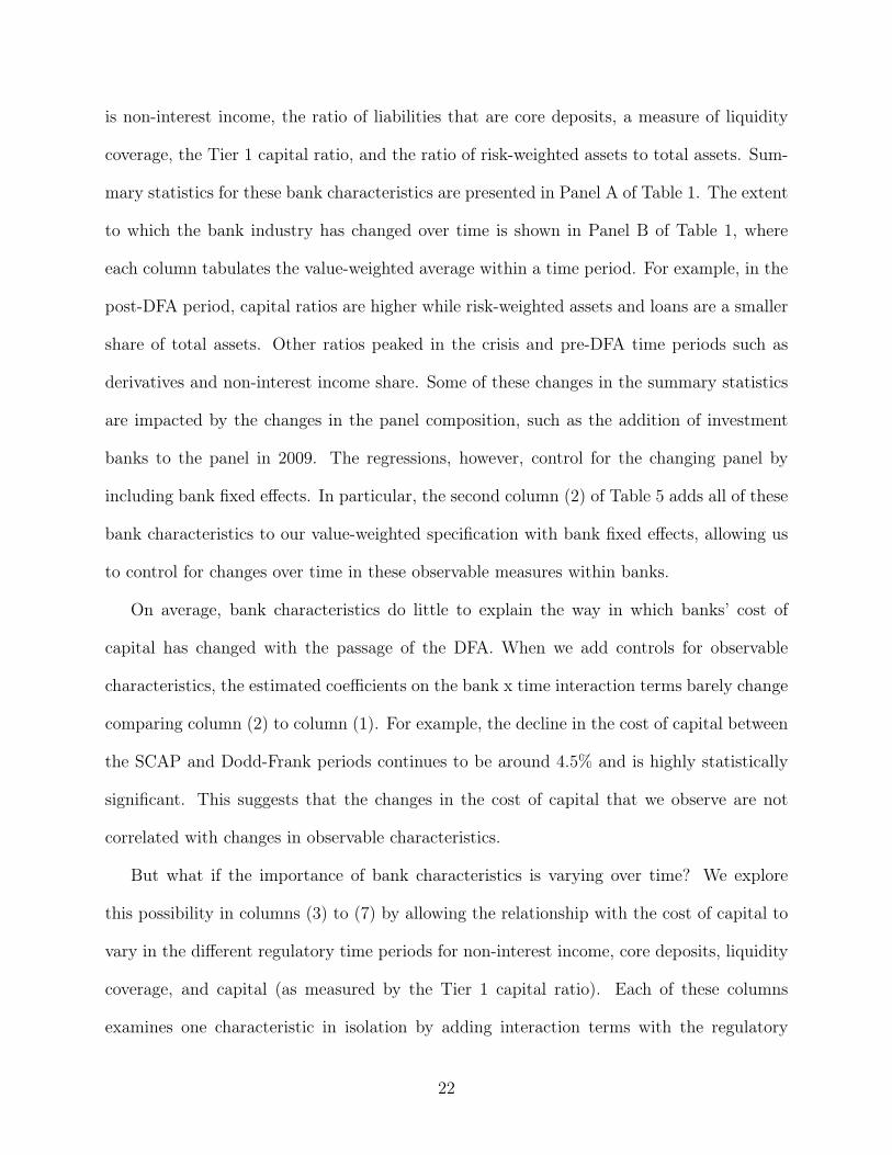
is non-interest income, the ratio of liabilities that are core deposits, a measure of liquidity

coverage, the Tier 1 capital ratio, and the ratio of risk-weighted assets to total assets. Sum-

mary statistics for these bank characteristics are presented in Panel A of Table 1. The extent

to which the bank industry has changed over time is shown in Panel B of Table 1, where

each column tabulates the value-weighted average within a time period. For example, in the

post-DFA period, capital ratios are higher while risk-weighted assets and loans are a smaller

share of total assets. Other ratios peaked in the crisis and pre-DFA time periods such as

derivatives and non-interest income share. Some of these changes in the summary statistics

are impacted by the changes in the panel composition, such as the addition of investment

banks to the panel in 2009. The regressions, however, control for the changing panel by

including bank fixed effects. In particular, the second column (2) of Table 5 adds all of these

bank characteristics to our value-weighted specification with bank fixed effects, allowing us

to control for changes over time in these observable measures within banks.

On average, bank characteristics do little to explain the way in which banks’ cost of

capital has changed with the passage of the DFA. When we add controls for observable

characteristics, the estimated coefficients on the bank x time interaction terms barely change

comparing column (2) to column (1). For example, the decline in the cost of capital between

the SCAP and Dodd-Frank periods continues to be around 4.5% and is highly statistically

significant. This suggests that the changes in the cost of capital that we observe are not

correlated with changes in observable characteristics.

But what if the importance of bank characteristics is varying over time? We explore

this possibility in columns (3) to (7) by allowing the relationship with the cost of capital to

vary in the different regulatory time periods for non-interest income, core deposits, liquidity

coverage, and capital (as measured by the Tier 1 capital ratio). Each of these columns

examines one characteristic in isolation by adding interaction terms with the regulatory

22

time periods so the coefficients can vary over time. The final specification (8) includes all of

the characteristics and their time period interactions together to highlight how the estimated

coefficients on the bank x time interactions change in comparison to column (1), although in

column (8) we do not report the characteristic x time interaction coefficients as in column

(2) for readability.

Consistent with Calomiris and Nissim (2014), the results in columns (3) to (6) indicate

that there has been some variation in the association between banks’ cost of capital and bank

characteristics across the regulatory time periods, but accounting for this time variation does

not reverse the general patterns in banks’ cost of capital after the financial crisis, such as

the decline after DFA. The results do change, however, after including risk-weighted assets

(RWA) in column (7). While there is no statistically significant relationship between RWA

and expected returns for most of the regulatory time periods, RWA emerges as a key driver

of banks’ cost of capital during the post-crisis SCAP period with a coefficient that is positive

and highly significant. Moreover, when this interaction is included, the difference between

the coefficients on the Bank x SCAP and Bank x Dodd-Frank indicators falls to almost

nothing and is no longer significant. This result suggests that after the financial crisis,

market expected returns for banks with higher RWA increased dramatically, and then fell

again after the passage of the DFA. As shown in the final specification (8) which incldes all

the interactions, RWA appears to be the key variable driving the change in the results.

The result for RWA appears to be driven by changes in the association between the

cost of capital and loans. We run similar regressions using key components of RWA such

as liquid assets (cash, fed funds, and securities), loans, trading assets, commitments, and

derivatives (results are in Appendix Table A.4). While none of the RWA components by itself

reverses the general patterns in banks’ cost of capital over time, the biggest changes in the

characteristic coefficients during the SCAP period occur for loans and loan commitments,

23

which both become significant and positive. Within loans, the coefficients on real estate loans

increase the most in SCAP period (not shown). This is consistent with a market increase in

expected returns for banks with more real estate loans and loan commitments in the SCAP

period that was subsequently reversed.

The time-varying association with RWA does not fully explain the decline in the cost

of capital for the largest banks (see Appendix Table A.5). Across specifications that in-

clude controls for time-varying bank characteristics, the cost of capital for the largest banks

continues to decline by 3% to 4% after the SCAP period. Since the largest banks are dif-

ferentially subject to increased regulation, these results are consistent with an increase in

regulation leading to lower risk and lower expected returns in the Dodd-Frank period. To

lend further weight to this interpretation, we extend the analysis by looking specifically at

a single regulatory change in the next section.

4.4 Stress tests

While it is hard to attribute changes in the cost of capital to particular regulations because

so many regulations were changed at the same time for the same set of firms, we attempt to

take advantage of the staggered implementation of stress testing on banks with more than

$50 billion in assets to understand how a particular regulatory change, stress testing, may

have affected the cost of capital for stress-tested banks. Table 6 presents the results of this

analysis. Rather than using an indicator for banks, the panel includes only the 90 largest

banks by assets each month that have regulatory data and then use separate indicators for

the sets of banks that became subject to stress testing at different times.12

12Note that not all firms that are stress tested are publicly traded – we exclude from the analysis the bankswith foreign parents, and Ally and Citizens join the panel only after IPO. Because of its bankruptcy andsubsequent reorganization, we exclude CIT from the panel entirely. If included, it would be the only bankin its category, since it was added to stress testing in 2016, and it would be in the comparison, non-stresstested group before that time. Similarly, we exclude Metlife from the panel entirely due to its subsequentdebanking.

24

On average, the cost of capital increases for the large banks in this panel relative to the

pre-period. The coefficients on the time periods are all positive and statistically significantly

different from zero. Relative to the pre-period, the cost of capital is 7% higher after SCAP,

4% higher after the DFA is passed and prior to the initial disclosure of stress testing results

in 2012, and 3.5% higher in the post stress testing CCAR period. Figure 3 illustrates these

results by plotting the equal-weighted cost of capital for the SCAP, CCAR, and other banks

in the top 90 by asset size. The plot indicates that the largest increase in the cost of

capital during the financial crisis and subsequent decline post-DFA occurs for the SCAP

firms relative to the other large banks. Table 6 formalizes these results. The last rows

include SCAP firm x time period interactions that allow the coefficients for SCAP firms to

differ from other large banks after 2009 and a CCAR firm x Post-CCAR coefficient that

allows CCAR firms to differ in the post stress testing CCAR period (specifications 2-4, 6-8).

We find that, while SCAP firm’s cost of capital increased by 2 percentage points during the

SCAP period, their cost of capital fell after DFA and then continued to decline by 150 basis

points in the post stress testing CCAR period relative to other large banks (specification

3). This within-firm decline of more than 3% since the SCAP period is significant at the

1% level and robust to including bank characteristics as unconditional control variables as

in Table 5. Similar to prior results, we include all controls in the regression and only report

the coefficient on the Tier 1 Capital ratio for readability (specification 4).

The results indicate that the largest reduction in the cost of capital occurs for the very

largest stress-tested banks. This means that stress testing has differentially reduced systemic

risk for the very largest firms. While we think that the staggered introduction of firms to

stress testing contributes identifying power, we cannot distinguish this hypothesis from the

alternative explanation that it reflects other regulations to which only these very largest firms

are subject have also been implemented with timing similar to that of CCAR. Generally,

25

since the cost of capital estimates in our approach require time to estimate betas, we think it

is difficult to identify changes in time windows shorter than those captured in this analysis.

5 The cost of capital and lending supply and pricing

While the CAPM costs of capital estimates are interesting on their own as measures of the

systematic risk of banks as captured in equity market prices, in this section we motivate our

interest in CAPM by examining the real effects of the changes in the cost of capital. Since we

are interested in documenting the co-movement of the cost of capital at individual banks with

bank lending supply, rather than more general co-movements driven by the business cycle,

we focus on a cost of capital measure that nets out the risk free rate. We find that lending

standards and the cost of capital move together – Figure 4 plots the the average change

in credit standards for large and middle-market firms against the average one-year change

in the CAPM risk premium less the risk-free rate for the banks in the SLOOS survey. In

aggregate, these variables are positively correlated and the average response to the business

cycle is procyclical, with banks tightening standards during recessions and easing standards

during expansions. We make use of the confidential bank-level data to examine this result in

the cross-section while controlling for changes over time through quarterly time fixed effects.

This approach increases power, controls for the business cycle, and identifies a relationship

between bank-level credit standards and changes in the cost of capital net of the risk-free

rate.

5.1 Changes in lending standards and the cost of capital

Table 7 reports the results of this analysis in Panel A which presents a set of regressions

of quarterly changes in lending standards (Std) as measured by survey responses in the

26

SLOOS onto one-year changes in the cost of capital net of the risk-free rate, similar to

the approach described in equation 6. The first three columns examine the relationship for

the largest borrowers, while the second three columns look at responses to questions about

smaller borrowers. We estimate a positive and significant coefficient on the change in the

cost of capital indicating that bank managers are tightening credit standards when their

cost of capital net of the risk-free rate is increasing. To interpret the magnitude of the

point estimate, an increase in a bank’s CAPM beta from 1 to 2 would increase the cost of

capital risk premium by 8% which translates into a 8 x .024 = 0.19 higher survey response,

about one-fifth the magnitude of an increase from one category of the response to another

or about one-half the standard deviation of the dependent variable which equals .47. When

a bank’s cost of capital increases, lending standards are tightened. The effect is larger for

large borrowers, although the difference is not statistically significant in all specifications.

We want to be sure that we are not just capturing variation in the business cycle or the

impact of idiosyncratic bank shocks. To account for this, we add one-year changes in the risk-

free rate and one-year bank-level stock market returns as control variables (specification 2).

Including bank-level stock market returns is a challenging test for omitted variable bias that

allows us to capture the extent to which a negative shock from bad loans or poor profits may

contribute to tighter lending standards. As expected, we estimate a negative and significant

relationship between loan standards and both control variables. When interest rates decline

or bank stock returns are low, lending standards are tighter. Adding these controls reduces

the coefficient on the change in the CAPM cost of capital by half, but it does not reverse

the result. An increase in the CAPM cost of capital remains significantly and positively

associated with tighter loan standards. Interpreting the magnitude of the coefficients, a one-

standard deviation change in the cost of capital, risk-free rate, and realized return results in

a .03, .15, and .06 change in lending standards (specification 2). Bank managers appear to

27

tighten credit standards when the cost of capital risk premium (∆ CAPM - Rf) increases,

even after controlling for changes in the risk-free rate and for firm-level stock market returns.

Finally, we illustrate that the results are robust to including quarterly fixed effects (spec-

ification 3), a more comprehensive control for any time-varying shock that would affect

bank lending supply. These time fixed effects increase the explanatory power from 14% to

26%, indicating the importance of robust controls for changes in the business cycle variation

including the aggregate tightening of spreads during the financial crisis. Despite this, the

change in the cost of capital remains significant with a similar magnitude to the second spec-

ification. The results are largely similar although of slightly smaller magnitudes for smaller

borrowers (specifications 4-6).

5.2 Changes in lending terms and the cost of capital

In panels B and C of Table 7, we go beyond broad lending standards and look separately at

the effect of changes in the cost of capital on different lending terms covered in the SLOOS

questions such as: the cost of credit lines, the spread of loan rates over bank’s cost of funds,

the premiums charged on riskier loans, loan covenants, collateralization requirements, and

the maximum size of credit lines. Each of these terms is a dependent variable in the different

columns of Panel B (larger borrowers) and C (small borrowers). Since we found that quarterly

fixed effects contribute substantial explanatory power, we include quarter fixed effects in all

the specifications, similar to the third specification from Panel A. We find that increases

in banks’ cost of capital are associated with tightening in the supply and pricing of credit

through all of the lending terms measured, with greater statistical and economic significance

for larger borrowers. The estimated relationship is generally positive but not significant for

smaller borrowers.

The spread of loan rates over a bank’s cost of funds and the premiums charged on riskier

28

loans are perhaps the survey responses that most directly relate to the cost of capital. Indeed,

we estimate the largest relationship between changes in the cost of capital and the response

to these questions. When a bank’s CAPM beta increases from 1 to 2, senior loan officers

report a 0.14 to 0.12 higher survey response on average for loan spreads and premiums on

riskier loans, about one-fifth of one standard deviation of the survey response. In addition

to these impacts on loan prices, we also find that banks decrease the maximum size of

credit lines and tighten loan covenants when their cost of capital increases, thereby reducing

credit supply. The results for collateral requirements are similar but not significant. These

varied findings highlight the rich nature of the SLOOS data. Rather than being restricted to

only study the quantity and pricing of loans through quarterly changes in loan balances or

interest margins in call report data, the SLOOS allows us to investigate the provision of credit

along multiple dimensions from the perspective of senior loan officers who are responsible

for allocating credit in the economy. Building on the prior literature that has documented

a negative relationship between the cost of capital and investment for non-financials, our

results provide new evidence that banks act in a similar fashion, tightening the supply and

pricing of credit in the economy when their CAPM cost of capital increases.

6 Alternative cost of capital estimates

In general, misspecification of expected returns that is associated with our regulatory time

periods could bias our results. The advantage of multifactor models is to potentially better

measure expected returns, thereby reducing any bias. To understand the robustness of

the results for the CAPM cost of capital, Table 8 repeats the key difference-in-differences

specifications for banks and top banks for different cost of capital estimates including three-

factor estimates following Fama and French (1993), five-factor estimates that incorporate

29

additional interest rate and term spread factors, one-factor estimates with a time-varying

equity risk premium, log CAPM betas that difference out the equity risk premium, and

asset betas from the Merton (1974) model. Across the various estimates we consistently find

a significant decrease in the cost of capital for the largest banks since the passage of the

DFA. Figure 5 summarizes these results by plotting the value-weighted alternative cost of

capital estimates alongside our estimates of asset betas and market leverage for the banking

sector. As before, while the plot may be affected by the changing composition of the panel,

we control for this in the regressions with firm fixed effects and document significant within

firm changes over time.

6.1 Multifactor cost of capital estimates

The Fama and French (1993) three-factor model (FF3) delivers cost of capital estimates

that account for the variation in expected returns for small versus big firms and for value

versus growth firms. As before, we define the FF3 cost of capital as the sum of time-varying

betas multiplied by constant factor risk premiums. We set the factor risk premiums equal

to the average excess returns for the tradeable factors from 1926 to 2017 which are equal to

8%, 4.6%, and 2.5% in annualized units for the market, size, and value factors respectively.

The average beta or loading on these factors for banks over the last twenty years has been

1.17 (0.54), 0.85 (0.43), -0.11 (0.41) respectively versus 1.17 (0.55) for the CAPM on a

value-weighted (equal-weighted) basis.

Columns (1) and (2) of Table 8 repeat the value-weighted difference-in-differences regres-

sions with firm fixed effects from Tables 3 and 4 for banks and top banks. Compared to

the previous results, the FF3 model indicates that banks’ cost of capital diverged the most

from non-banks in the period immediately preceding the financial crisis, when value factor

betas were declining and banks were trading more like growth firms, rather than exhibiting

30

a decline in the period immediately following the crisis. Another difference is the Bank

x Dodd-Frank coefficient, which indicates that banks have exhibited a 1% decline in their

within-firm FF3 cost of capital (column 1) versus generally positive and significant estimates

for the CAPM model. This fall in the cost of capital is driven by the largest banks, as shown

in the results in column (2). For the top banks, the FF3 cost of capital has differentially

fallen since the passage of the DFA by about 3%, similar to the CAPM regressions. More-

over, the Bank x Top x Dodd-Frank coefficient is large in economic magnitude and highly

significant, indicating that the FF3 cost of capital has differentially declined for the largest

banks relative to the pre-GLB period as well. These results are stronger than the Top regres-

sions for the CAPM which also feature negative coefficients on Bank x Top x Current but

with magnitudes that are smaller and less significant. By capturing the changing loadings

on the value and size factors during the financial crisis, the FF3 analysis indicates that the

cost of capital for the largest banks has differentially fallen by as much as 3% relative to

both the pre-GLB period and since the passage of the DFA.

In addition to size and value, other factors that affect expected stock returns for banks

differently from other companies and that are correlated with the business cycle have the

potential to bias our results. One such factor may be changes in interest rates, as maturity

transformation and interest rate risk management are key aspects of bank business models,

but may be less important for non-bank firms. To that end, we form a five-factor model (IR)

that adds a short-term interest rate factor and a yield curve slope factor to the three-factor

model. Columns (3) and (4) of Table 8 report the results. To maintain consistency with our

prior results, we use tradeable interest rate factors that are constructed from zero-coupon

bond prices using the yield curve from Gurkaynak et al. (2006).13 Having controlled for

13The interest rate factors are Rshort,t = R2y,t − Rf,t and Rslope,t = 15 (R10y,t − Rf,t) − (R2y,t − Rf,t)

where R2y,t and R10y,t are the daily return for two-year and ten-year zero coupon bonds and Rf,t is the dailyrisk-free rate. The slope factor has zero duration by construction and is -99% (-74%) correlated with thechange in the 10y-2y zero-coupon (constant maturity) slope at a daily frequency. The short term factor is

31

interest rates in this manner, we confirm our CAPM cost of capital finding that banks exhibit

a large and significant decrease in their cost of capital after the passage of the DFA relative

to both the SCAP and pre-GLB periods. The decrease of approximately 4.5% relative to the

pre-GLB period is large relative to both the CAPM and FF3 models (column 3). The Top

regression confirms that the largest banks are driving this result, with a differential decline

of 3% relative to the SCAP period and 5% relative to the pre-GLB period (column 4).

6.2 CAPM with a time-varying equity risk premium

A time-varying risk premium that is correlated with bank betas may bias our results. For

example, if bank betas and the equity risk premium both increased in the Crisis and SCAP

periods and then declined in the Dodd-Frank period, our estimate of the decline in the cost

of capital for banks assuming a constant risk premium will be underestimated, all else equal.

To address this concern we consider two approaches. First, we use a model to estimate

the equity risk premium and then repeat our analysis for the CAPM with this time-varying

risk premium. To do this, we form a one-factor partial least squares estimate of the equity

risk premium by combining 14 models of the equity risk premium from Duarte and Rosa

(2015) with available data from 1965 to 2016.14 We then project one-year ahead CRSP

value-weighted returns onto the partial least squares estimate and use the fitted value as

a measure of the equity risk premium. This approach has the advantage that it directly

addresses the concern that the equity risk premium is time varying but the disadvantage

that the results are model and sample dependent.

For an alternative perspective, we take advantage of the fact that the equity risk premium

-99% (-94%) correlated with the change in the 2y zero-coupon (constant maturity) yield at a daily frequency.The average factor risk premiums from 1975 to 2017 are µshort = 1.14% and µslope = −.41% (the averageannualized excess return for the 10-year zero coupon bond is 3.67%).

14Similar results hold by projecting one-year ahead returns onto the estimate of the equity risk premiumfrom a dividend discount model, which is one of the 14 models included in the partial least squares estimate.

32

drops out of a difference-in-differences analysis after taking the logarithm since the CAPM

is a one-factor model.15 We thus estimate our difference-in-differences regressions using the

logarithm of the CAPM betas as the dependent variable. We implement this idea empirically

by winsorizing the estimated betas at .05 to remove negative values from the sample.

Table 8 reports the baseline regressions for the CAPM using the partial least squares

estimate of the equity risk premium (PLS-Rf) and for the logarithm of the CAPM betas

(Log(Beta)).16 For the PLS-Rf regressions almost all of the time period coefficients are larger

than those in the specifications with a constant risk premium. This reflects the fact that

our estimate of the time-varying equity risk premium has increased over the sample period,

consistent with the findings in Duarte and Rosa (2015). For banks, the results are generally

consistent with those from other CAPM specifications, in that the estimated cost of capital is

higher in the Dodd-Frank period relative to the pre-GLB period but significantly lower than

the SCAP period. Column (5) indicates that the cost of capital for banks has declined by

around 9% from the SCAP period to the Dodd-Frank period. Column (6) shows that these

results are again driven by the very largest banks. In comparison to the previous results,

the larger magnitudes suggest that the assumption of a constant equity risk premium may

be biasing our results down. Equivalently, the results suggest that bank betas are positively

correlated with the equity risk premium.

Similar results also hold when taking the logarithm of the CAPM betas as the dependent

variable in columns (7) and (8). For example, columns (7) and (8) indicate that bank CAPM

betas have declined by about 35% from SCAP to Dodd-Frank with much of the decline being

driven by the largest banks. One difference from the PLS-Rf results in column (6) is the

15In particular, log(βi,tµt) − log(βi,t−1µt−1) − (log(βj,tµt)− log(βj,t−1µt−1)) = log(βi,t) − log(βi,t−1) −(log(βj,t)− log(βj,t−1)) . This argument does not apply to multifactor models.

16The PLS-Rf results are from March 1996 to 2016 when the equity risk premium estimates are availablefrom Duarte and Rosa (2015). This results in a slightly smaller sample and contrasts the other regressionswhich end in 2017.

33

negative and significant coefficient on Bank x Top x Dodd-Frank in column (8). The negative

coefficient for log betas is consistent with the CAPM, three-factor, and five-factor cost of

capital estimates using constant factor risk premiums which all indicate that the cost of

capital for the largest banks has declined relative to both the pre-GLB and SCAP periods

on a within firm, value-weighted basis.

6.3 Asset betas

The key component driving changes in our cost of capital estimates is the estimate of eq-

uity betas. In this way, the analysis captures changes to the systematic risk of the banking

industry. However, since these estimates are affected by leverage we may also be interested

in looking directly at asset betas, which may better capture the systematic risk of banking

assets, regardless of capital structure changes. We compute asset betas in the Merton (1974)

model using equity market capitalization and equity volatility for each firm-month observa-

tion in the sample following the approach in Bharath and Shumway (2008).17 This analysis

directly incorporates leverage into the estimated beta rather than including leverage as a

linear control variable in reduced form regressions as in Table 4 (specification 5) or in Table

5 (specification 6) (where leverage is included as a time-varying characteristic as measured

by the Tier 1 capital ratio). The disadvantage of this approach is that the computation of

asset betas is model specific and requires a number of assumptions, such as how to compute

the maturity and face value of debt. These assumptions may be particularly important for

banks.

Columns (9) and (10) in Table 8 report the results with asset beta as the dependent

17We compute asset betas by solving for firm value and volatility from two nonlinear equations for thevalue of equity and equity volatility, similar to how the default probability πsimul

Merton is computed in Bharathand Shumway (2008). To do this we assume that debt matures in one year and define the face value ofdebt as short-term debt plus one-half long-term debt plus deposits if available. In a previous draft we foundsimilar results by assuming that debt was riskless as in Baker and Wurgler (2015) in which case asset betasare equal to βasset

i,t = βi,t(1− Li,t) where Li,t = Di,t/(Di,t +MEi,t).

34

variable. Looking at the bank interaction coefficients on the regulatory time periods, we still

estimate a significant decrease in banks’ asset betas between the SCAP and Dodd-Frank

periods that is primarily driven by the very largest banks. This result is noteworthy as the

significant decline persists despite the decrease in bank leverage in recent years, which would

imply increased asset betas of banks if equity betas were unchanged. From a longer historical

perspective, bank asset betas have increased relative to the pre-GLB period by around .10

as measured by the significant and positive Bank x Top x Dodd-Frank coefficient in column

(10). This result differs from the cost of capital estimates which generally feature a negative

difference for the largest banks.

6.4 Weighted average cost of capital

In communications with investors and employees, bank managers reference ROE targets

which are often compared the cost of equity capital. Pennacchi and Santos (2018) document

that bank stocks appear to respond to ROE changes. However, given that banks are heavily

financed with debt and deposits, an equity based measure may not capture the average (nor

marginal) financing cost for a bank.

Therefore, we repeat our analysis for the weighted average cost of capital (WACC),

another commonly used measure of the cost of capital that takes into account the after-tax

cost of debt, the cost of equity, and the capital structure. We estimate WACC from merged

CRSP-Compustat data as,

WACCi,t = Rei,t ·MEi,t

Di,t +MEi,t+Rdi,t · (1− τi,t) ·

Di,t

Di,t +MEi,t, (7)

where Rei,t is the cost of equity capital as estimated in equation 1, Rdi,t is the cost of

debt, τi,t is the effective tax rate, Di,t is total debt, MEi,t is market equity, and Li,t =

35

Di,t/(Di,t + MEi,t) is market leverage.18 When defining total debt for banks, we add the

total amount of deposits to capture this important component of bank leverage. The resulting

leverage in the Dodd-Frank period is 0.81 for banks and 0.19 for non-banks (see Table 1 for

changes in leverage across periods). Note also that our cost of debt measure is based on

accounting data so may adjust slowly over time. This differs from our estimates of the cost

of equity capital which are based on market prices, but is consistent with empirical evidence

on sticky deposit pricing.

Table 9 reports the difference-in-differences regressions using WACC-Rf as the dependent

variable. The first column (1) indicates that value-weighted WACC-Rf has increased by

about 1% over the past twenty years for all firms. The second column (2) indicates that

bank WACC-Rf is almost 6% lower than non-bank WACC-Rf on average, reflecting the

high leverage and low interest rates of banks relative to non-banks. Similar to the previous

results, the second (2) and third (3) columns also indicate that WACC-Rf has fallen for

banks between the SCAP and Dodd-Frank periods by around 1%, but increased between

the Dodd-Frank and pre-GLB periods by around 1.5%. For the Top banks we see a further

decrease in WACC-Rf by around 20 to 30 basis points in the specifications with firm fixed

effects and the equal-weighted regression without fixed effects (specifications 5, 6, 7), but

an increase in the value-weighted regression without fixed effects of around 15 basis points.

In contrast to the previous results, the changes for Top Banks are not significant when

comparing the SCAP and Dodd-Frank periods, although we still see a decline across most

18The cost of debt is a one-year moving average of quarterly interest expense over total debt which includesdeposits. Total debt is long-term debt (Item DLTTQ) plus short-term debt (Item DLCQ) plus deposits ifavailable (Item DPTCQ). Depending on availability, we use Item XINTQ or Item TIEQ in that order forquarterly interest expense. The effective tax rate is a one-year moving median of quarterly income taxes(Item TXTQ) over pre-tax income (Item PIQ). We winsorize the cost of debt, the effective tax rate, andmarket leverage at the 1% and 99% percentiles to mitigate the impact of outliers and measurement error.This data cleaning step is performed separately for financials and non-financials each month to allow fordifferences in firm characteristics and time trends, such as the high leverage of financial firms and the lowercost of debt and tax rates in recent years.

36

specifications. For the cost of equity capital we consistently found a large and significant

decline across specifications when comparing the SCAP and Dodd-Frank periods.

7 Conclusion

Banks’ cost of capital is an input into decisions about lending quantities and pricing as well

as decisions regarding resource allocation to different business lines. This paper rigorously

estimates the cost of capital for the banking industry and explores how it has changed over

time. After spiking in the financial crisis, the cost of capital for the banking industry has

fallen dramatically since the passage of the Dodd-Frank Act. Expected returns for the very

largest banks most affected by regulation have fallen differentially by 1% to 3% relative

to post-financial crisis highs depending on the metric. Since these measures are driven by

changes in equity and asset betas, this means that the systematic risk of these firms has

fallen since the passage of the Dodd-Frank Act. For the largest banks in particular, there

has been a differential decline relative to both the financial crisis and relative to the late

1990s across different measures and regression specifications. This is striking in the face of

research such as Atkeson et al. (2018) that suggests that the value of government guarantees

are falling over the same period of time.

While these results suggest that the systematic risk of banks has declined in the post

Dodd-Frank era, it is worth noting the limitations of any analysis that seeks to understand

the cost of capital. The true cost of capital measure relevant to bank managers is the

unobserved expected returns of bank investors. Bank managers and econometricians do

not have a time series of expected returns, only the models by which we estimate expected

returns. Any test is thus a joint test of changes to expected returns and of the model

for estimating expected returns. Some issues are alleviated by the differences-in-differences

37

approach. For example, the risk-free rate is added to the expected returns and thus drops

out when differencing. Changes in banks’ cost of capital can be compared to other industries

using different models, even if it is difficult to precisely estimate the level of banks’ cost of

capital itself.

Ultimately, these questions are not just of academic interest. Our estimates of the cost

of capital are capturing changes in market prices that matter to bank managers as reflected

by changes in bank lending supply. The evidence suggests that the CAPM cost of capital

for banks matters over and above changes in the risk free rates – increases in CAPM cost of

capital are associated with tighter lending conditions, pricing, and quantity.

38

ReferencesAdmati, A. R., P. M. DeMarzo, M. F. Hellwig, and P. C. Pfleiderer (2014). Fallacies and irrelevant facts in

the debate on capital regulation. In Central Banks at a Crossroads: Europe and Beyond, pp. 33–50.London: Anthem Press.

Adrian, T., E. Friedman, and T. Muir (2015). The cost of capital of the financial sector. Federal ReserveBank of New York Staff Report .

Ang, A. and D. Kristensen (2012). Testing conditional factor models. Journal of FinancialEconomics 106 (1), 132–156.

Atkeson, A. G., A. d’Avernas, A. L. Eisfeldt, and P.-O. Weill (2018). Government guarantees and thevaluation of american banks. NBER Macroeconomics Annual .

Baker, M. and J. Wurgler (2015). Do strict capital requirements raise the cost of capital? bank regulation,capital structure, and the low-risk anomaly. American Economic Review: Papers & Proceedings 105 (5),315–320.

Bassett, W. F., M. B. Chosak, J. C. Driscoll, and E. Zakrajšek (2014). Changes in bank lending standardsand the macroeconomy. Journal of Monetary Economics 62, 23–40.

Berk, J. B. and J. H. van Binsbergen (2016). Assessing asset pricing models using revealed preference.Journal of Financial Economics 119 (1), 1–23.

Bharath, S. T. and T. Shumway (2008). Forecasting default with the merton distance to default model.The Review of Financial Studies 21 (3), 1339–1369.

Black, F., M. C. Jensen, and M. S. Scholes (1972). The capital asset pricing model: Some empirical tests.In M. C. Jensen (Ed.), Studies in the Theory of Capital Markets, pp. 79–121. New York, NY: Praeger.

Calomiris, C. W. and D. Nissim (2014). Crisis-related shifts in the market valuation of banking activities.Journal of Financial Intermediation 23, 400–435.

Cochrane, J. H. (2011). Presidential address: Discount rates. The Journal of Finance 66 (4), 1047–1108.

Demsetz, R. S. and P. E. Strahan (1997). Diversification, size, and risk at bank holding companies. Journalof Money, Credit, and Banking 29 (3), 300–313.

DeYoung, R., A. Gron, G. Torna, and A. Winton (2015). Risk overhang and loan portfolio decisions: smallbusiness loan supply before and during the financial crisis. The Journal of Finance 70 (6), 2451–2488.

Duarte, F. and C. Rosa (2015). The equity risk premium: A review of models. Federal Reserve Bank ofNew York Economic Policy Review 21 (2), 39–57.

Fama, E. F. (1970). Efficient capital markets: A review of theory and empirical work. The Journal ofFinance 25 (2), 383–417.

Fama, E. F. and K. R. French (1993). Common risk factors in the returns on stocks and bonds. Journal ofFinancial Economics 33 (1), 3–56.

Fama, E. F. and K. R. French (1997). Industry costs of equity. Journal of Financial Economics 43 (2),153–193.

Flannery, M., B. Hirtle, and A. Kovner (2017). Evaluating the information in the federal reserve stresstests. Journal of Financial Intermediation 29, 1–18.

39

Frank, M. Z. and T. Shen (2016). Investment and the weighted average cost of capital. Journal ofFinancial Economics 119 (2), 300–315.

Frazzini, A. and L. H. Pedersen (2014). Betting against beta. Journal of Financial Economics 111 (1),1–25.

Gandhi, P. and H. Lustig (2015). Size anomalies in u.s. bank stock returns. The Journal of Finance 70 (2),733–768.

Gilchrist, S., J. W. Sim, and E. Zakrajšek (2013). Misallocation and financial market frictions: Some directevidence from the dispersion in borrowing costs. Review of Economic Dynamics 16 (1), 159–176.

Gilson, S. C., E. S. Hotchkiss, and R. S. Ruback (2000). Valuation of bankrupt firms. The Review ofFinancial Studies 13 (1), 43–74.

Graham, J. R. and C. R. Harvey (2001). The theory and practice of corporate finance: evidence from thefield. Journal of Financial Economics 60 (2-3), 187–243.

Gurkaynak, R., B. Sack, and J. Wright (2006). The us treasury curve: 1961 to present. Journal ofMonetary Economics 54 (8), 2291–2304.

Hale, G. and J. Santos (2014). Do banks propagate shocks to the debt market? Journal of FinancialEconomic Policy 6 (3), 270–310.

Harvey, C. R., Y. Liu, and H. Zhu (2016). . . . and the cross-section of expected returns. The Review ofFinancial Studies 29 (1), 5–68.

Hirtle, B. (2009). Credit derivatives and bank credit supply. Journal of Financial Intermediation 18 (2),125–150.

Hou, K., C. Xue, and L. Zhang (2014). Digesting anomalies: An investment approach. Review of FinancialStudies 28 (3), 650–704.

Huizinga, H. and L. Laeven (2012). Bank valuation and accounting discretion during a financial crisis.Journal of Financial Economics 106 (3), 614–634.

Kelly, B., H. Lustig, and S. Van Nieuwerburgh (2016). Too-systemic-to-fail: What option markets implyabout sector-wide government guarantees. American Economic Review 106 (6), 1278–1319.

Linnainmaa, J. T. and M. R. Roberts (2016). The history of the cross section of stock returns. SSRN .

Lown, C. and D. P. Morgan (2006). The credit cycle and the business cycle: New findings using the loanofficer opinion survey. Journal of Money, Credit and Banking 38 (6), 1575–1597.

Merton, R. C. (1974). On the pricing of corporate debt: The risk structure of interest rates. The Journalof Finance 29 (2), 449–470.

Merton, R. C. (1980). On estimating the expected return on the market: An exploratory investigation.Journal of Financial Economics 8 (4), 323–361.

Minton, B. A., R. M. Stulz, and A. G. Taboada (2017). Are larger banks valued more highly? SSRN .

Modigliani, F. and M. H. Miller (1958). The cost of capital, corporation finance and the theory ofinvestment. American Economic Review 48 (3), 261–297.

Pennacchi, G. and J. A. Santos (2018). Why do banks target roe? Working Paper .

Philippon, T. (2009). The bond market’s q. The Quarterly Journal of Economics 124 (3), 1011–1056.

40

Sarin, N. and L. H. Summers (2016). Understanding bank risk through market measures. Brookings Paperson Economic Activity , 57–127.

Scholes, M. and J. Williams (1977). Estimating betas from nonsynchronous data. Journal of FinancialEconomics 5 (3), 309–327.

Schuermann, T. and K. J. Stiroh (2006). Visible and hidden risk factors for banks. Federal Reserve Bank ofNew York Staff Report .

Welch, I. and A. Goyal (2007). A comprehensive look at the empirical performance of equity premiumprediction. The Review of Financial Studies 21 (4), 1455–1508.

41

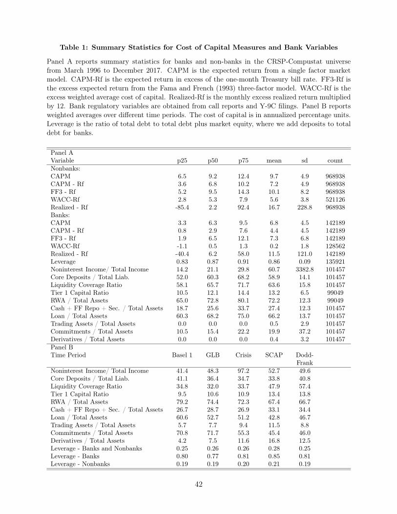
Table 1: Summary Statistics for Cost of Capital Measures and Bank Variables

Panel A reports summary statistics for banks and non-banks in the CRSP-Compustat universefrom March 1996 to December 2017. CAPM is the expected return from a single factor marketmodel. CAPM-Rf is the expected return in excess of the one-month Treasury bill rate. FF3-Rf isthe excess expected return from the Fama and French (1993) three-factor model. WACC-Rf is theexcess weighted average cost of capital. Realized-Rf is the monthly excess realized return multipliedby 12. Bank regulatory variables are obtained from call reports and Y-9C filings. Panel B reportsweighted averages over different time periods. The cost of capital is in annualized percentage units.Leverage is the ratio of total debt to total debt plus market equity, where we add deposits to totaldebt for banks.

Panel AVariable p25 p50 p75 mean sd countNonbanks:CAPM 6.5 9.2 12.4 9.7 4.9 968938CAPM - Rf 3.6 6.8 10.2 7.2 4.9 968938FF3 - Rf 5.2 9.5 14.3 10.1 8.2 968938WACC-Rf 2.8 5.3 7.9 5.6 3.8 521126Realized - Rf -85.4 2.2 92.4 16.7 228.8 968938Banks:CAPM 3.3 6.3 9.5 6.8 4.5 142189CAPM - Rf 0.8 2.9 7.6 4.4 4.5 142189FF3 - Rf 1.9 6.5 12.1 7.3 6.8 142189WACC-Rf -1.1 0.5 1.3 0.2 1.8 128562Realized - Rf -40.4 6.2 58.0 11.5 121.0 142189Leverage 0.83 0.87 0.91 0.86 0.09 135921Noninterest Income/ Total Income 14.2 21.1 29.8 60.7 3382.8 101457Core Deposits / Total Liab. 52.0 60.3 68.2 58.9 14.1 101457Liquidity Coverage Ratio 58.1 65.7 71.7 63.6 15.8 101457Tier 1 Capital Ratio 10.5 12.1 14.4 13.2 6.5 99049RWA / Total Assets 65.0 72.8 80.1 72.2 12.3 99049Cash + FF Repo + Sec. / Total Assets 18.7 25.6 33.7 27.4 12.3 101457Loan / Total Assets 60.3 68.2 75.0 66.2 13.7 101457Trading Assets / Total Assets 0.0 0.0 0.0 0.5 2.9 101457Commitments / Total Assets 10.5 15.4 22.2 19.9 37.2 101457Derivatives / Total Assets 0.0 0.0 0.0 0.4 3.2 101457Panel BTime Period Basel 1 GLB Crisis SCAP Dodd-

FrankNoninterest Income/ Total Income 41.4 48.3 97.2 52.7 49.6Core Deposits / Total Liab. 41.1 36.4 34.7 33.8 40.8Liquidity Coverage Ratio 34.8 32.0 33.7 47.9 57.4Tier 1 Capital Ratio 9.5 10.6 10.9 13.4 13.8RWA / Total Assets 79.2 74.4 72.3 67.4 66.7Cash + FF Repo + Sec. / Total Assets 26.7 28.7 26.9 33.1 34.4Loan / Total Assets 60.6 52.7 51.2 42.8 46.7Trading Assets / Total Assets 5.7 7.7 9.4 11.5 8.8Commitments / Total Assets 70.8 71.7 55.3 45.4 46.0Derivatives / Total Assets 4.2 7.5 11.6 16.8 12.5Leverage - Banks and Nonbanks 0.25 0.26 0.26 0.28 0.25Leverage - Banks 0.80 0.77 0.81 0.85 0.81Leverage - Nonbanks 0.19 0.19 0.20 0.21 0.19

42

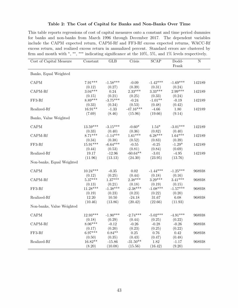
Table 2: The Cost of Capital for Banks and Non-Banks Over Time

This table reports regressions of cost of capital measures onto a constant and time period dummiesfor banks and non-banks from March 1996 through December 2017. The dependent variablesinclude the CAPM expected return, CAPM-Rf and FF3-Rf excess expected returns, WACC-Rfexcess return, and realized excess return in annualized percent. Standard errors are clustered byfirm and month with ∗, ∗∗, ∗∗∗ indicating significance at the 10%, 5%, and 1% levels respectively.

Cost of Capital Measure Constant GLB Crisis SCAP Dodd-Frank

N

Banks, Equal Weighted

CAPM 7.91*** -1.58*** -0.09 -1.42*** -1.69*** 142189(0.12) (0.27) (0.39) (0.31) (0.24)

CAPM-Rf 3.04*** 0.24 2.33*** 3.33*** 2.99*** 142189(0.15) (0.21) (0.25) (0.33) (0.24)

FF3-Rf 8.89*** -3.75*** -0.24 -1.01** -0.19 142189(0.33) (0.34) (0.53) (0.48) (0.42)

Realized-Rf 16.91** -1.33 -47.16*** -4.66 1.80 142189(7.69) (8.46) (15.96) (19.66) (9.14)

Banks, Value Weighted

CAPM 13.59*** -3.15*** -0.60* 1.54* -3.01*** 142189(0.33) (0.40) (0.36) (0.82) (0.40)

CAPM-Rf 8.71*** -1.14*** 1.61*** 6.28*** 1.64*** 142189(0.34) (0.38) (0.52) (0.83) (0.39)

FF3-Rf 15.91*** -6.64*** -0.55 -0.25 -1.29* 142189(0.44) (0.53) (0.81) (0.84) (0.69)

Realized-Rf 19.17 -12.96 -60.64** -3.01 -4.95 142189(11.96) (13.13) (24.30) (23.95) (13.76)

Non-banks, Equal Weighted

CAPM 10.24*** -0.35 0.02 -1.44*** -1.25*** 968938(0.12) (0.25) (0.44) (0.18) (0.16)

CAPM-Rf 5.37*** 1.37*** 2.38*** 3.29*** 3.41*** 968938(0.13) (0.21) (0.18) (0.19) (0.15)

FF3-Rf 11.28*** -1.38*** -2.38*** -1.08*** -1.57*** 968938(0.19) (0.23) (0.23) (0.22) (0.20)

Realized-Rf 12.20 10.50 -24.18 31.67 6.08 968938(10.46) (13.86) (20.42) (22.66) (11.93)

Non-banks, Value Weighted

CAPM 12.93*** -1.90*** -2.74*** -5.02*** -4.91*** 968938(0.18) (0.29) (0.44) (0.25) (0.22)

CAPM-Rf 8.06*** -0.12 -0.26 -0.28 -0.26 968938(0.17) (0.20) (0.23) (0.25) (0.22)

FF3-Rf 6.97*** 0.84** 0.25 0.76 0.42 968938(0.50) (0.35) (0.43) (0.47) (0.48)

Realized-Rf 16.82** -15.86 -31.50** 1.82 -1.17 968938(8.20) (10.08) (15.56) (16.42) (9.20)

43

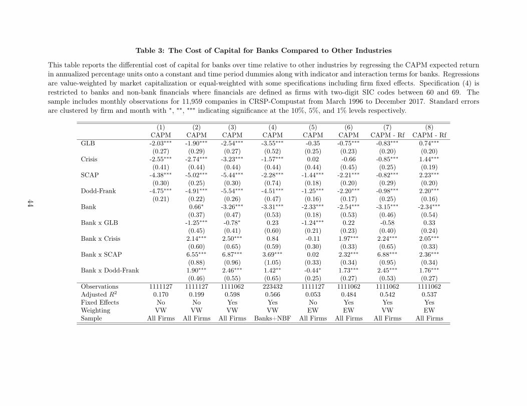
Table 3: The Cost of Capital for Banks Compared to Other Industries

This table reports the differential cost of capital for banks over time relative to other industries by regressing the CAPM expected returnin annualized percentage units onto a constant and time period dummies along with indicator and interaction terms for banks. Regressionsare value-weighted by market capitalization or equal-weighted with some specifications including firm fixed effects. Specification (4) isrestricted to banks and non-bank financials where financials are defined as firms with two-digit SIC codes between 60 and 69. Thesample includes monthly observations for 11,959 companies in CRSP-Compustat from March 1996 to December 2017. Standard errorsare clustered by firm and month with ∗, ∗∗, ∗∗∗ indicating significance at the 10%, 5%, and 1% levels respectively.

(1) (2) (3) (4) (5) (6) (7) (8)CAPM CAPM CAPM CAPM CAPM CAPM CAPM - Rf CAPM - Rf

GLB -2.03∗∗∗ -1.90∗∗∗ -2.54∗∗∗ -3.55∗∗∗ -0.35 -0.75∗∗∗ -0.83∗∗∗ 0.74∗∗∗(0.27) (0.29) (0.27) (0.52) (0.25) (0.23) (0.20) (0.20)

Crisis -2.55∗∗∗ -2.74∗∗∗ -3.23∗∗∗ -1.57∗∗∗ 0.02 -0.66 -0.85∗∗∗ 1.44∗∗∗(0.41) (0.44) (0.44) (0.44) (0.44) (0.45) (0.25) (0.19)

SCAP -4.38∗∗∗ -5.02∗∗∗ -5.44∗∗∗ -2.28∗∗∗ -1.44∗∗∗ -2.21∗∗∗ -0.82∗∗∗ 2.23∗∗∗(0.30) (0.25) (0.30) (0.74) (0.18) (0.20) (0.29) (0.20)

Dodd-Frank -4.75∗∗∗ -4.91∗∗∗ -5.54∗∗∗ -4.51∗∗∗ -1.25∗∗∗ -2.20∗∗∗ -0.98∗∗∗ 2.20∗∗∗(0.21) (0.22) (0.26) (0.47) (0.16) (0.17) (0.25) (0.16)

Bank 0.66∗ -3.26∗∗∗ -3.31∗∗∗ -2.33∗∗∗ -2.54∗∗∗ -3.15∗∗∗ -2.34∗∗∗(0.37) (0.47) (0.53) (0.18) (0.53) (0.46) (0.54)

Bank x GLB -1.25∗∗∗ -0.78∗ 0.23 -1.24∗∗∗ 0.22 -0.58 0.33(0.45) (0.41) (0.60) (0.21) (0.23) (0.40) (0.24)

Bank x Crisis 2.14∗∗∗ 2.50∗∗∗ 0.84 -0.11 1.97∗∗∗ 2.24∗∗∗ 2.05∗∗∗(0.60) (0.65) (0.59) (0.30) (0.33) (0.65) (0.33)

Bank x SCAP 6.55∗∗∗ 6.87∗∗∗ 3.69∗∗∗ 0.02 2.32∗∗∗ 6.88∗∗∗ 2.36∗∗∗(0.88) (0.96) (1.05) (0.33) (0.34) (0.95) (0.34)

Bank x Dodd-Frank 1.90∗∗∗ 2.46∗∗∗ 1.42∗∗ -0.44∗ 1.73∗∗∗ 2.45∗∗∗ 1.76∗∗∗(0.46) (0.55) (0.65) (0.25) (0.27) (0.53) (0.27)

Observations 1111127 1111127 1111062 223432 1111127 1111062 1111062 1111062Adjusted R2 0.170 0.199 0.598 0.566 0.053 0.484 0.542 0.537Fixed Effects No No Yes Yes No Yes Yes YesWeighting VW VW VW VW EW EW VW EWSample All Firms All Firms All Firms Banks+NBF All Firms All Firms All Firms All Firms

44

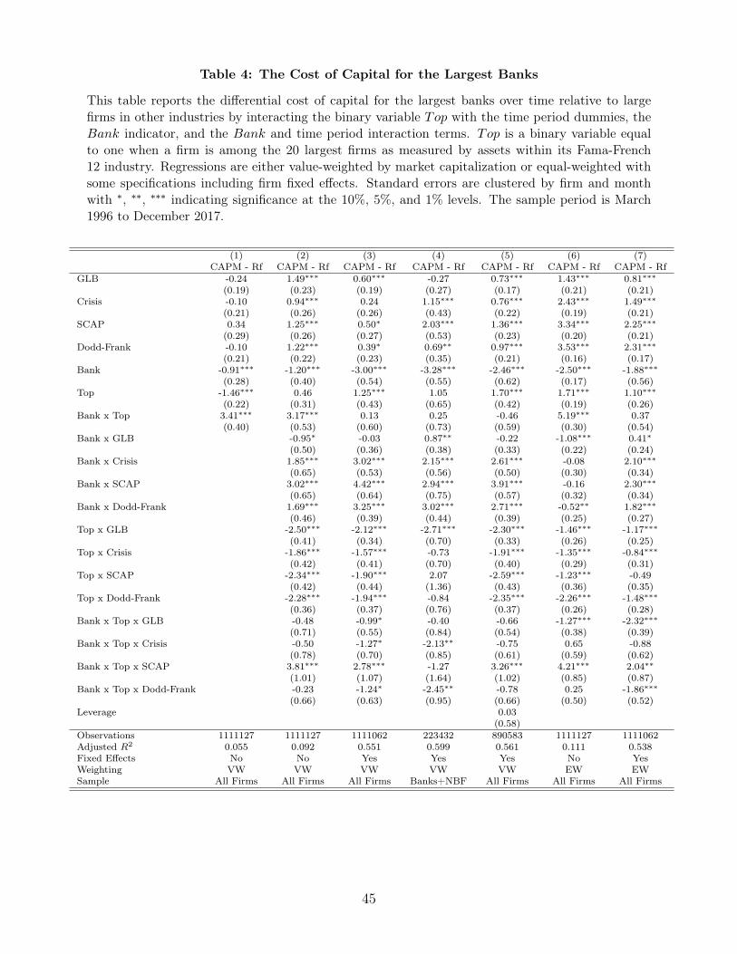
Table 4: The Cost of Capital for the Largest Banks

This table reports the differential cost of capital for the largest banks over time relative to largefirms in other industries by interacting the binary variable Top with the time period dummies, theBank indicator, and the Bank and time period interaction terms. Top is a binary variable equalto one when a firm is among the 20 largest firms as measured by assets within its Fama-French12 industry. Regressions are either value-weighted by market capitalization or equal-weighted withsome specifications including firm fixed effects. Standard errors are clustered by firm and monthwith ∗, ∗∗, ∗∗∗ indicating significance at the 10%, 5%, and 1% levels. The sample period is March1996 to December 2017.

(1) (2) (3) (4) (5) (6) (7)CAPM - Rf CAPM - Rf CAPM - Rf CAPM - Rf CAPM - Rf CAPM - Rf CAPM - Rf

GLB -0.24 1.49∗∗∗ 0.60∗∗∗ -0.27 0.73∗∗∗ 1.43∗∗∗ 0.81∗∗∗(0.19) (0.23) (0.19) (0.27) (0.17) (0.21) (0.21)

Crisis -0.10 0.94∗∗∗ 0.24 1.15∗∗∗ 0.76∗∗∗ 2.43∗∗∗ 1.49∗∗∗(0.21) (0.26) (0.26) (0.43) (0.22) (0.19) (0.21)

SCAP 0.34 1.25∗∗∗ 0.50∗ 2.03∗∗∗ 1.36∗∗∗ 3.34∗∗∗ 2.25∗∗∗(0.29) (0.26) (0.27) (0.53) (0.23) (0.20) (0.21)

Dodd-Frank -0.10 1.22∗∗∗ 0.39∗ 0.69∗∗ 0.97∗∗∗ 3.53∗∗∗ 2.31∗∗∗(0.21) (0.22) (0.23) (0.35) (0.21) (0.16) (0.17)

Bank -0.91∗∗∗ -1.20∗∗∗ -3.00∗∗∗ -3.28∗∗∗ -2.46∗∗∗ -2.50∗∗∗ -1.88∗∗∗(0.28) (0.40) (0.54) (0.55) (0.62) (0.17) (0.56)

Top -1.46∗∗∗ 0.46 1.25∗∗∗ 1.05 1.70∗∗∗ 1.71∗∗∗ 1.10∗∗∗(0.22) (0.31) (0.43) (0.65) (0.42) (0.19) (0.26)

Bank x Top 3.41∗∗∗ 3.17∗∗∗ 0.13 0.25 -0.46 5.19∗∗∗ 0.37(0.40) (0.53) (0.60) (0.73) (0.59) (0.30) (0.54)

Bank x GLB -0.95∗ -0.03 0.87∗∗ -0.22 -1.08∗∗∗ 0.41∗(0.50) (0.36) (0.38) (0.33) (0.22) (0.24)

Bank x Crisis 1.85∗∗∗ 3.02∗∗∗ 2.15∗∗∗ 2.61∗∗∗ -0.08 2.10∗∗∗(0.65) (0.53) (0.56) (0.50) (0.30) (0.34)

Bank x SCAP 3.02∗∗∗ 4.42∗∗∗ 2.94∗∗∗ 3.91∗∗∗ -0.16 2.30∗∗∗(0.65) (0.64) (0.75) (0.57) (0.32) (0.34)

Bank x Dodd-Frank 1.69∗∗∗ 3.25∗∗∗ 3.02∗∗∗ 2.71∗∗∗ -0.52∗∗ 1.82∗∗∗(0.46) (0.39) (0.44) (0.39) (0.25) (0.27)

Top x GLB -2.50∗∗∗ -2.12∗∗∗ -2.71∗∗∗ -2.30∗∗∗ -1.46∗∗∗ -1.17∗∗∗(0.41) (0.34) (0.70) (0.33) (0.26) (0.25)

Top x Crisis -1.86∗∗∗ -1.57∗∗∗ -0.73 -1.91∗∗∗ -1.35∗∗∗ -0.84∗∗∗(0.42) (0.41) (0.70) (0.40) (0.29) (0.31)

Top x SCAP -2.34∗∗∗ -1.90∗∗∗ 2.07 -2.59∗∗∗ -1.23∗∗∗ -0.49(0.42) (0.44) (1.36) (0.43) (0.36) (0.35)

Top x Dodd-Frank -2.28∗∗∗ -1.94∗∗∗ -0.84 -2.35∗∗∗ -2.26∗∗∗ -1.48∗∗∗(0.36) (0.37) (0.76) (0.37) (0.26) (0.28)

Bank x Top x GLB -0.48 -0.99∗ -0.40 -0.66 -1.27∗∗∗ -2.32∗∗∗(0.71) (0.55) (0.84) (0.54) (0.38) (0.39)

Bank x Top x Crisis -0.50 -1.27∗ -2.13∗∗ -0.75 0.65 -0.88(0.78) (0.70) (0.85) (0.61) (0.59) (0.62)

Bank x Top x SCAP 3.81∗∗∗ 2.78∗∗∗ -1.27 3.26∗∗∗ 4.21∗∗∗ 2.04∗∗(1.01) (1.07) (1.64) (1.02) (0.85) (0.87)

Bank x Top x Dodd-Frank -0.23 -1.24∗ -2.45∗∗ -0.78 0.25 -1.86∗∗∗(0.66) (0.63) (0.95) (0.66) (0.50) (0.52)

Leverage 0.03(0.58)

Observations 1111127 1111127 1111062 223432 890583 1111127 1111062Adjusted R2 0.055 0.092 0.551 0.599 0.561 0.111 0.538Fixed Effects No No Yes Yes Yes No YesWeighting VW VW VW VW VW EW EWSample All Firms All Firms All Firms Banks+NBF All Firms All Firms All Firms

45

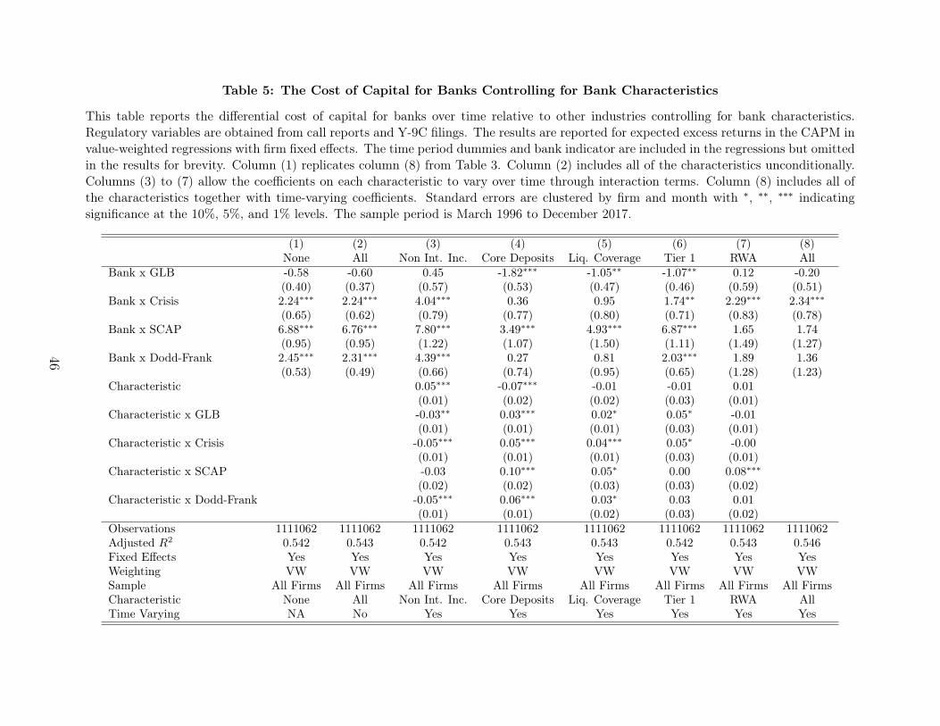
Table 5: The Cost of Capital for Banks Controlling for Bank Characteristics

This table reports the differential cost of capital for banks over time relative to other industries controlling for bank characteristics.Regulatory variables are obtained from call reports and Y-9C filings. The results are reported for expected excess returns in the CAPM invalue-weighted regressions with firm fixed effects. The time period dummies and bank indicator are included in the regressions but omittedin the results for brevity. Column (1) replicates column (8) from Table 3. Column (2) includes all of the characteristics unconditionally.Columns (3) to (7) allow the coefficients on each characteristic to vary over time through interaction terms. Column (8) includes all ofthe characteristics together with time-varying coefficients. Standard errors are clustered by firm and month with ∗, ∗∗, ∗∗∗ indicatingsignificance at the 10%, 5%, and 1% levels. The sample period is March 1996 to December 2017.

(1) (2) (3) (4) (5) (6) (7) (8)None All Non Int. Inc. Core Deposits Liq. Coverage Tier 1 RWA All

Bank x GLB -0.58 -0.60 0.45 -1.82∗∗∗ -1.05∗∗ -1.07∗∗ 0.12 -0.20(0.40) (0.37) (0.57) (0.53) (0.47) (0.46) (0.59) (0.51)

Bank x Crisis 2.24∗∗∗ 2.24∗∗∗ 4.04∗∗∗ 0.36 0.95 1.74∗∗ 2.29∗∗∗ 2.34∗∗∗(0.65) (0.62) (0.79) (0.77) (0.80) (0.71) (0.83) (0.78)

Bank x SCAP 6.88∗∗∗ 6.76∗∗∗ 7.80∗∗∗ 3.49∗∗∗ 4.93∗∗∗ 6.87∗∗∗ 1.65 1.74(0.95) (0.95) (1.22) (1.07) (1.50) (1.11) (1.49) (1.27)

Bank x Dodd-Frank 2.45∗∗∗ 2.31∗∗∗ 4.39∗∗∗ 0.27 0.81 2.03∗∗∗ 1.89 1.36(0.53) (0.49) (0.66) (0.74) (0.95) (0.65) (1.28) (1.23)

Characteristic 0.05∗∗∗ -0.07∗∗∗ -0.01 -0.01 0.01(0.01) (0.02) (0.02) (0.03) (0.01)

Characteristic x GLB -0.03∗∗ 0.03∗∗∗ 0.02∗ 0.05∗ -0.01(0.01) (0.01) (0.01) (0.03) (0.01)

Characteristic x Crisis -0.05∗∗∗ 0.05∗∗∗ 0.04∗∗∗ 0.05∗ -0.00(0.01) (0.01) (0.01) (0.03) (0.01)

Characteristic x SCAP -0.03 0.10∗∗∗ 0.05∗ 0.00 0.08∗∗∗(0.02) (0.02) (0.03) (0.03) (0.02)

Characteristic x Dodd-Frank -0.05∗∗∗ 0.06∗∗∗ 0.03∗ 0.03 0.01(0.01) (0.01) (0.02) (0.03) (0.02)

Observations 1111062 1111062 1111062 1111062 1111062 1111062 1111062 1111062Adjusted R2 0.542 0.543 0.542 0.543 0.543 0.542 0.543 0.546Fixed Effects Yes Yes Yes Yes Yes Yes Yes YesWeighting VW VW VW VW VW VW VW VWSample All Firms All Firms All Firms All Firms All Firms All Firms All Firms All FirmsCharacteristic None All Non Int. Inc. Core Deposits Liq. Coverage Tier 1 RWA AllTime Varying NA No Yes Yes Yes Yes Yes Yes

46

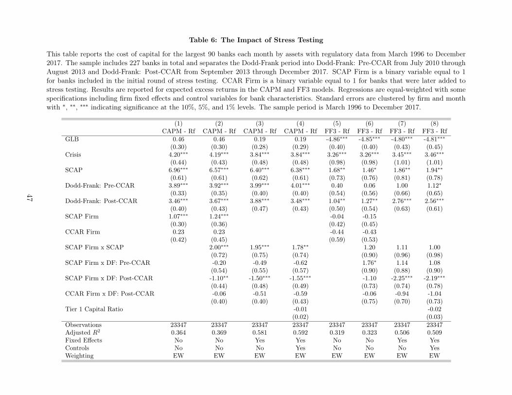
Table 6: The Impact of Stress Testing

This table reports the cost of capital for the largest 90 banks each month by assets with regulatory data from March 1996 to December2017. The sample includes 227 banks in total and separates the Dodd-Frank period into Dodd-Frank: Pre-CCAR from July 2010 throughAugust 2013 and Dodd-Frank: Post-CCAR from September 2013 through December 2017. SCAP Firm is a binary variable equal to 1for banks included in the initial round of stress testing. CCAR Firm is a binary variable equal to 1 for banks that were later added tostress testing. Results are reported for expected excess returns in the CAPM and FF3 models. Regressions are equal-weighted with somespecifications including firm fixed effects and control variables for bank characteristics. Standard errors are clustered by firm and monthwith ∗, ∗∗, ∗∗∗ indicating significance at the 10%, 5%, and 1% levels. The sample period is March 1996 to December 2017.

(1) (2) (3) (4) (5) (6) (7) (8)CAPM - Rf CAPM - Rf CAPM - Rf CAPM - Rf FF3 - Rf FF3 - Rf FF3 - Rf FF3 - Rf

GLB 0.46 0.46 0.19 0.19 -4.86∗∗∗ -4.85∗∗∗ -4.80∗∗∗ -4.81∗∗∗(0.30) (0.30) (0.28) (0.29) (0.40) (0.40) (0.43) (0.45)

Crisis 4.20∗∗∗ 4.19∗∗∗ 3.84∗∗∗ 3.84∗∗∗ 3.26∗∗∗ 3.26∗∗∗ 3.45∗∗∗ 3.46∗∗∗(0.44) (0.43) (0.48) (0.48) (0.98) (0.98) (1.01) (1.01)

SCAP 6.96∗∗∗ 6.57∗∗∗ 6.40∗∗∗ 6.38∗∗∗ 1.68∗∗ 1.46∗ 1.86∗∗ 1.94∗∗(0.61) (0.61) (0.62) (0.61) (0.73) (0.76) (0.81) (0.78)

Dodd-Frank: Pre-CCAR 3.89∗∗∗ 3.92∗∗∗ 3.99∗∗∗ 4.01∗∗∗ 0.40 0.06 1.00 1.12∗(0.33) (0.35) (0.40) (0.40) (0.54) (0.56) (0.66) (0.65)

Dodd-Frank: Post-CCAR 3.46∗∗∗ 3.67∗∗∗ 3.88∗∗∗ 3.48∗∗∗ 1.04∗∗ 1.27∗∗ 2.76∗∗∗ 2.56∗∗∗(0.40) (0.43) (0.47) (0.43) (0.50) (0.54) (0.63) (0.61)

SCAP Firm 1.07∗∗∗ 1.24∗∗∗ -0.04 -0.15(0.30) (0.36) (0.42) (0.45)

CCAR Firm 0.23 0.23 -0.44 -0.43(0.42) (0.45) (0.59) (0.53)

SCAP Firm x SCAP 2.00∗∗∗ 1.95∗∗∗ 1.78∗∗ 1.20 1.11 1.00(0.72) (0.75) (0.74) (0.90) (0.96) (0.98)

SCAP Firm x DF: Pre-CCAR -0.20 -0.49 -0.62 1.76∗ 1.14 1.08(0.54) (0.55) (0.57) (0.90) (0.88) (0.90)

SCAP Firm x DF: Post-CCAR -1.10∗∗ -1.50∗∗∗ -1.55∗∗∗ -1.10 -2.25∗∗∗ -2.19∗∗∗(0.44) (0.48) (0.49) (0.73) (0.74) (0.78)

CCAR Firm x DF: Post-CCAR -0.06 -0.51 -0.59 -0.06 -0.94 -1.04(0.40) (0.40) (0.43) (0.75) (0.70) (0.73)

Tier 1 Capital Ratio -0.01 -0.02(0.02) (0.03)

Observations 23347 23347 23347 23347 23347 23347 23347 23347Adjusted R2 0.364 0.369 0.581 0.592 0.319 0.323 0.506 0.509Fixed Effects No No Yes Yes No No Yes YesControls No No No Yes No No No YesWeighting EW EW EW EW EW EW EW EW

47

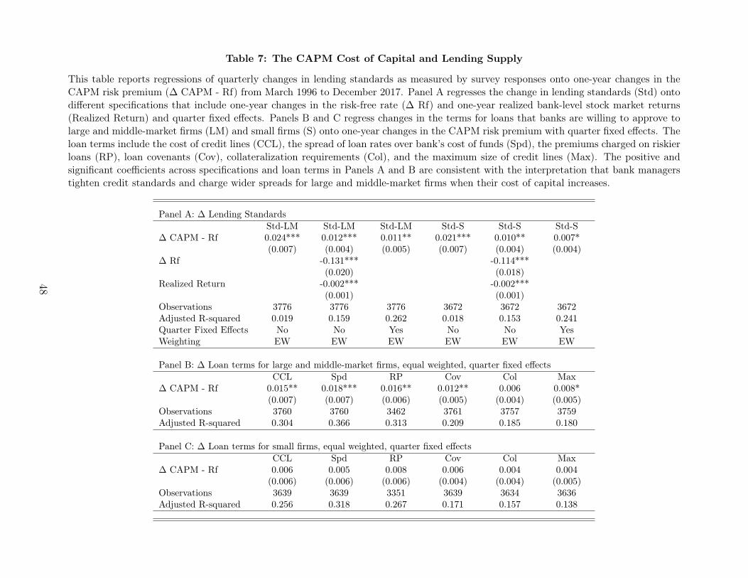
Table 7: The CAPM Cost of Capital and Lending Supply

This table reports regressions of quarterly changes in lending standards as measured by survey responses onto one-year changes in theCAPM risk premium (∆ CAPM - Rf) from March 1996 to December 2017. Panel A regresses the change in lending standards (Std) ontodifferent specifications that include one-year changes in the risk-free rate (∆ Rf) and one-year realized bank-level stock market returns(Realized Return) and quarter fixed effects. Panels B and C regress changes in the terms for loans that banks are willing to approve tolarge and middle-market firms (LM) and small firms (S) onto one-year changes in the CAPM risk premium with quarter fixed effects. Theloan terms include the cost of credit lines (CCL), the spread of loan rates over bank’s cost of funds (Spd), the premiums charged on riskierloans (RP), loan covenants (Cov), collateralization requirements (Col), and the maximum size of credit lines (Max). The positive andsignificant coefficients across specifications and loan terms in Panels A and B are consistent with the interpretation that bank managerstighten credit standards and charge wider spreads for large and middle-market firms when their cost of capital increases.

Panel A: ∆ Lending StandardsStd-LM Std-LM Std-LM Std-S Std-S Std-S

∆ CAPM - Rf 0.024*** 0.012*** 0.011** 0.021*** 0.010** 0.007*(0.007) (0.004) (0.005) (0.007) (0.004) (0.004)

∆ Rf -0.131*** -0.114***(0.020) (0.018)

Realized Return -0.002*** -0.002***(0.001) (0.001)

Observations 3776 3776 3776 3672 3672 3672Adjusted R-squared 0.019 0.159 0.262 0.018 0.153 0.241Quarter Fixed Effects No No Yes No No YesWeighting EW EW EW EW EW EW

Panel B: ∆ Loan terms for large and middle-market firms, equal weighted, quarter fixed effectsCCL Spd RP Cov Col Max

∆ CAPM - Rf 0.015** 0.018*** 0.016** 0.012** 0.006 0.008*(0.007) (0.007) (0.006) (0.005) (0.004) (0.005)

Observations 3760 3760 3462 3761 3757 3759Adjusted R-squared 0.304 0.366 0.313 0.209 0.185 0.180

Panel C: ∆ Loan terms for small firms, equal weighted, quarter fixed effectsCCL Spd RP Cov Col Max

∆ CAPM - Rf 0.006 0.005 0.008 0.006 0.004 0.004(0.006) (0.006) (0.006) (0.004) (0.004) (0.005)

Observations 3639 3639 3351 3639 3634 3636Adjusted R-squared 0.256 0.318 0.267 0.171 0.157 0.138

48

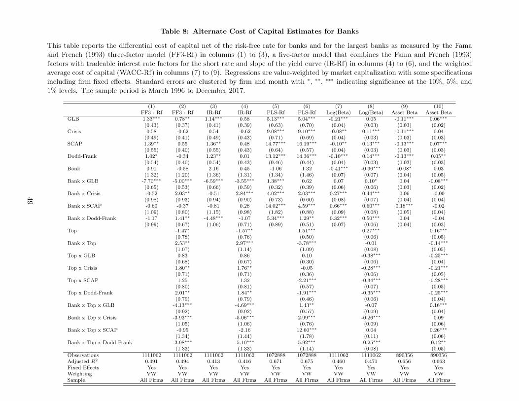
Table 8: Alternate Cost of Capital Estimates for Banks

This table reports the differential cost of capital net of the risk-free rate for banks and for the largest banks as measured by the Famaand French (1993) three-factor model (FF3-Rf) in columns (1) to (3), a five-factor model that combines the Fama and French (1993)factors with tradeable interest rate factors for the short rate and slope of the yield curve (IR-Rf) in columns (4) to (6), and the weightedaverage cost of capital (WACC-Rf) in columns (7) to (9). Regressions are value-weighted by market capitalization with some specificationsincluding firm fixed effects. Standard errors are clustered by firm and month with ∗, ∗∗, ∗∗∗ indicating significance at the 10%, 5%, and1% levels. The sample period is March 1996 to December 2017.

(1) (2) (3) (4) (5) (6) (7) (8) (9) (10)FF3 - Rf FF3 - Rf IR-Rf IR-Rf PLS-Rf PLS-Rf Log(Beta) Log(Beta) Asset Beta Asset Beta

GLB 1.33∗∗∗ 0.78∗∗ 1.14∗∗∗ 0.58 5.13∗∗∗ 5.04∗∗∗ -0.21∗∗∗ 0.05 -0.11∗∗∗ 0.06∗∗∗(0.43) (0.37) (0.41) (0.39) (0.63) (0.70) (0.04) (0.03) (0.03) (0.02)

Crisis 0.58 -0.62 0.54 -0.62 9.08∗∗∗ 9.10∗∗∗ -0.08∗∗ 0.11∗∗∗ -0.11∗∗∗ 0.04(0.49) (0.41) (0.49) (0.43) (0.71) (0.69) (0.04) (0.03) (0.03) (0.03)

SCAP 1.39∗∗ 0.55 1.36∗∗ 0.48 14.77∗∗∗ 16.19∗∗∗ -0.10∗∗ 0.13∗∗∗ -0.13∗∗∗ 0.07∗∗∗(0.55) (0.40) (0.55) (0.43) (0.64) (0.57) (0.04) (0.03) (0.03) (0.03)

Dodd-Frank 1.02∗ -0.34 1.23∗∗ 0.01 13.12∗∗∗ 14.36∗∗∗ -0.10∗∗∗ 0.14∗∗∗ -0.13∗∗∗ 0.05∗∗(0.54) (0.40) (0.54) (0.43) (0.46) (0.44) (0.04) (0.03) (0.03) (0.03)

Bank 0.91 -0.58 2.16 0.45 -1.06 1.32 -0.41∗∗∗ -0.36∗∗∗ -0.08∗ 0.03(1.32) (1.20) (1.36) (1.31) (1.34) (1.46) (0.07) (0.07) (0.04) (0.05)

Bank x GLB -7.70∗∗∗ -5.00∗∗∗ -6.59∗∗∗ -3.55∗∗∗ 1.38∗∗∗ 0.62 0.07 0.10∗ 0.04 -0.08∗∗∗(0.65) (0.53) (0.66) (0.59) (0.32) (0.39) (0.06) (0.06) (0.03) (0.02)

Bank x Crisis -0.52 2.03∗∗ -0.51 2.84∗∗∗ 4.02∗∗∗ 2.03∗∗∗ 0.27∗∗∗ 0.44∗∗∗ 0.06 -0.00(0.98) (0.93) (0.94) (0.90) (0.73) (0.60) (0.08) (0.07) (0.04) (0.04)

Bank x SCAP -0.60 -0.37 -0.81 0.28 14.02∗∗∗ 4.59∗∗∗ 0.66∗∗∗ 0.60∗∗∗ 0.18∗∗∗ -0.02(1.09) (0.80) (1.15) (0.98) (1.82) (0.88) (0.09) (0.08) (0.05) (0.04)

Bank x Dodd-Frank -1.17 1.41∗∗ -4.48∗∗∗ -1.07 5.34∗∗∗ 1.29∗∗ 0.32∗∗∗ 0.50∗∗∗ 0.04 -0.04(0.99) (0.67) (1.06) (0.71) (0.89) (0.51) (0.07) (0.06) (0.04) (0.03)

Top -1.47∗ -1.57∗∗ 1.51∗∗∗ 0.27∗∗∗ 0.16∗∗∗(0.78) (0.76) (0.50) (0.06) (0.05)

Bank x Top 2.53∗∗ 2.97∗∗∗ -3.78∗∗∗ -0.01 -0.14∗∗∗(1.07) (1.14) (1.09) (0.08) (0.05)

Top x GLB 0.83 0.86 0.10 -0.38∗∗∗ -0.25∗∗∗(0.68) (0.67) (0.30) (0.06) (0.04)

Top x Crisis 1.80∗∗ 1.76∗∗ -0.05 -0.28∗∗∗ -0.21∗∗∗(0.71) (0.71) (0.36) (0.06) (0.05)

Top x SCAP 1.25 1.32 -2.21∗∗∗ -0.34∗∗∗ -0.28∗∗∗(0.80) (0.81) (0.57) (0.07) (0.05)

Top x Dodd-Frank 2.01∗∗ 1.84∗∗ -1.91∗∗∗ -0.35∗∗∗ -0.25∗∗∗(0.79) (0.79) (0.46) (0.06) (0.04)

Bank x Top x GLB -4.13∗∗∗ -4.69∗∗∗ 1.43∗∗ -0.07 0.16∗∗∗(0.92) (0.92) (0.57) (0.09) (0.04)

Bank x Top x Crisis -3.93∗∗∗ -5.06∗∗∗ 2.99∗∗∗ -0.26∗∗∗ 0.09(1.05) (1.06) (0.76) (0.09) (0.06)

Bank x Top x SCAP -0.95 -2.16 12.60∗∗∗ 0.04 0.26∗∗∗(1.34) (1.44) (1.78) (0.11) (0.06)

Bank x Top x Dodd-Frank -3.98∗∗∗ -5.10∗∗∗ 5.92∗∗∗ -0.25∗∗∗ 0.12∗∗(1.33) (1.33) (1.14) (0.08) (0.05)

Observations 1111062 1111062 1111062 1111062 1072888 1072888 1111062 1111062 890356 890356Adjusted R2 0.491 0.494 0.413 0.416 0.671 0.675 0.460 0.471 0.656 0.663Fixed Effects Yes Yes Yes Yes Yes Yes Yes Yes Yes YesWeighting VW VW VW VW VW VW VW VW VW VWSample All Firms All Firms All Firms All Firms All Firms All Firms All Firms All Firms All Firms All Firms

49

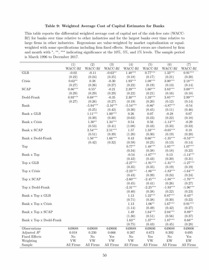
Table 9: Weighted Average Cost of Capital Estimates for Banks

This table reports the differential weighted average cost of capital net of the risk-free rate (WACC-Rf) for banks over time relative to other industries and for the largest banks over time relative tolarge firms in other industries. Regressions are value-weighted by market capitalization or equal-weighted with some specifications including firm fixed effects. Standard errors are clustered by firmand month with ∗, ∗∗, ∗∗∗ indicating significance at the 10%, 5%, and 1% levels. The sample periodis March 1996 to December 2017.

(1) (2) (3) (4) (5) (6) (7)WACC-Rf WACC-Rf WACC-Rf WACC-Rf WACC-Rf WACC-Rf WACC-Rf

GLB -0.02 -0.11 -0.63∗∗ 1.48∗∗∗ 0.77∗∗∗ 1.33∗∗∗ 0.91∗∗∗(0.22) (0.24) (0.25) (0.18) (0.17) (0.21) (0.20)

Crisis 0.62∗∗ 0.38 -0.30 1.93∗∗∗ 1.08∗∗∗ 3.00∗∗∗ 2.18∗∗∗(0.27) (0.26) (0.27) (0.22) (0.19) (0.13) (0.14)

SCAP 0.86∗∗∗ 0.55∗ -0.21 2.39∗∗∗ 1.60∗∗∗ 3.83∗∗∗ 3.00∗∗∗(0.29) (0.29) (0.29) (0.22) (0.21) (0.16) (0.18)

Dodd-Frank 0.93∗∗∗ 0.68∗∗∗ -0.35 2.30∗∗∗ 1.33∗∗∗ 3.85∗∗∗ 2.99∗∗∗(0.27) (0.26) (0.27) (0.19) (0.20) (0.12) (0.14)

Bank -5.94∗∗∗ -2.16∗∗∗ -5.54∗∗∗ -0.86∗ -4.87∗∗∗ -0.54(0.25) (0.42) (0.30) (0.45) (0.11) (0.46)

Bank x GLB 1.11∗∗∗ 1.00∗∗∗ 0.26 0.07 -0.28 0.07(0.39) (0.30) (0.62) (0.23) (0.22) (0.18)

Bank x Crisis 1.30∗∗ 1.34∗∗∗ 0.54 0.56 -1.14∗∗∗ -0.29(0.53) (0.41) (1.08) (0.43) (0.33) (0.33)

Bank x SCAP 2.54∗∗∗ 2.51∗∗∗ 1.57 1.33∗∗∗ -0.65∗∗∗ 0.18(0.51) (0.39) (1.20) (0.30) (0.19) (0.20)

Bank x Dodd-Frank 1.56∗∗∗ 1.66∗∗∗ 0.43 0.66∗∗∗ -1.35∗∗∗ -0.53∗∗∗(0.42) (0.32) (0.59) (0.25) (0.13) (0.14)

Top 0.77∗∗ 1.48∗∗∗ 1.05∗∗∗ 1.07∗∗∗(0.34) (0.38) (0.18) (0.22)

Bank x Top -0.54 -1.67∗∗∗ 0.13 -1.14∗∗∗(0.42) (0.43) (0.20) (0.31)

Top x GLB -2.27∗∗∗ -1.91∗∗∗ -1.31∗∗∗ -1.27∗∗∗(0.35) (0.35) (0.19) (0.19)

Top x Crisis -2.23∗∗∗ -1.86∗∗∗ -1.83∗∗∗ -1.64∗∗∗(0.43) (0.39) (0.24) (0.24)

Top x SCAP -2.60∗∗∗ -2.45∗∗∗ -1.88∗∗∗ -1.70∗∗∗(0.45) (0.41) (0.26) (0.27)

Top x Dodd-Frank -2.31∗∗∗ -2.25∗∗∗ -1.93∗∗∗ -1.96∗∗∗(0.40) (0.38) (0.22) (0.23)

Bank x Top x GLB 1.12 1.22∗∗∗ 0.87∗∗∗ 0.43∗∗(0.71) (0.38) (0.30) (0.22)

Bank x Top x Crisis 1.13 1.06∗∗ 1.67∗∗∗ 0.91∗∗∗(1.14) (0.49) (0.42) (0.27)

Bank x Top x SCAP 1.49 1.64∗∗∗ 2.04∗∗∗ 0.89∗∗(1.30) (0.51) (0.56) (0.37)

Bank x Top x Dodd-Frank 1.63∗∗ 1.37∗∗∗ 1.87∗∗∗ 0.68∗∗(0.75) (0.43) (0.45) (0.28)

Observations 649688 649688 649606 649688 649606 649688 649606Adjusted R2 0.018 0.230 0.666 0.267 0.673 0.392 0.695Fixed Effects No No Yes No Yes No YesWeighting VW VW VW VW VW EW EWSample All Firms All Firms All Firms All Firms All Firms All Firms All Firms

50

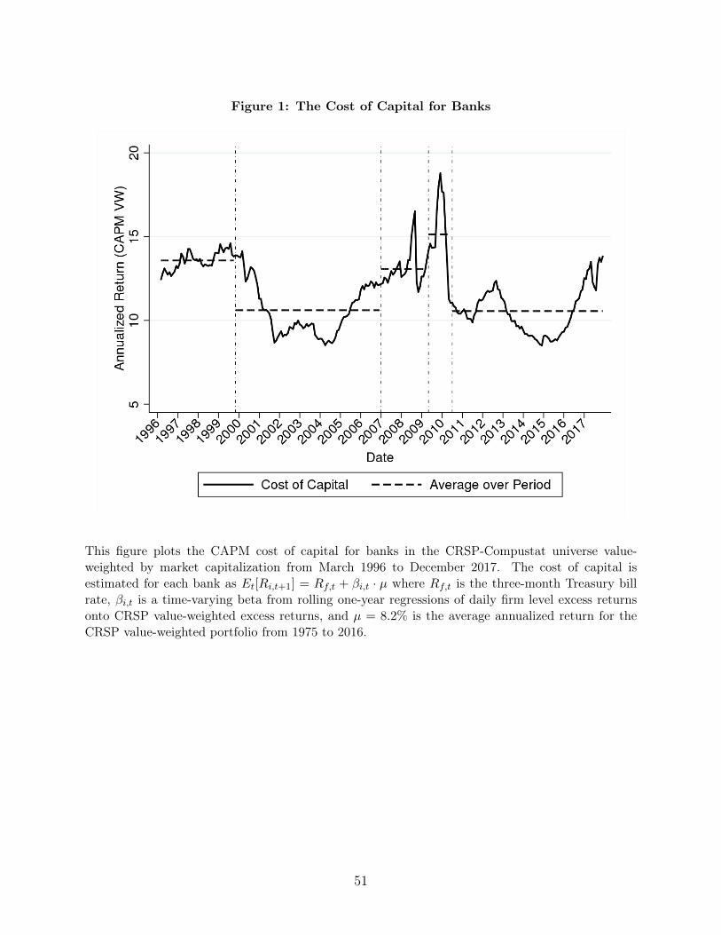
Figure 1: The Cost of Capital for Banks

This figure plots the CAPM cost of capital for banks in the CRSP-Compustat universe value-weighted by market capitalization from March 1996 to December 2017. The cost of capital isestimated for each bank as Et[Ri,t+1] = Rf,t + βi,t · µ where Rf,t is the three-month Treasury billrate, βi,t is a time-varying beta from rolling one-year regressions of daily firm level excess returnsonto CRSP value-weighted excess returns, and µ = 8.2% is the average annualized return for theCRSP value-weighted portfolio from 1975 to 2016.

51

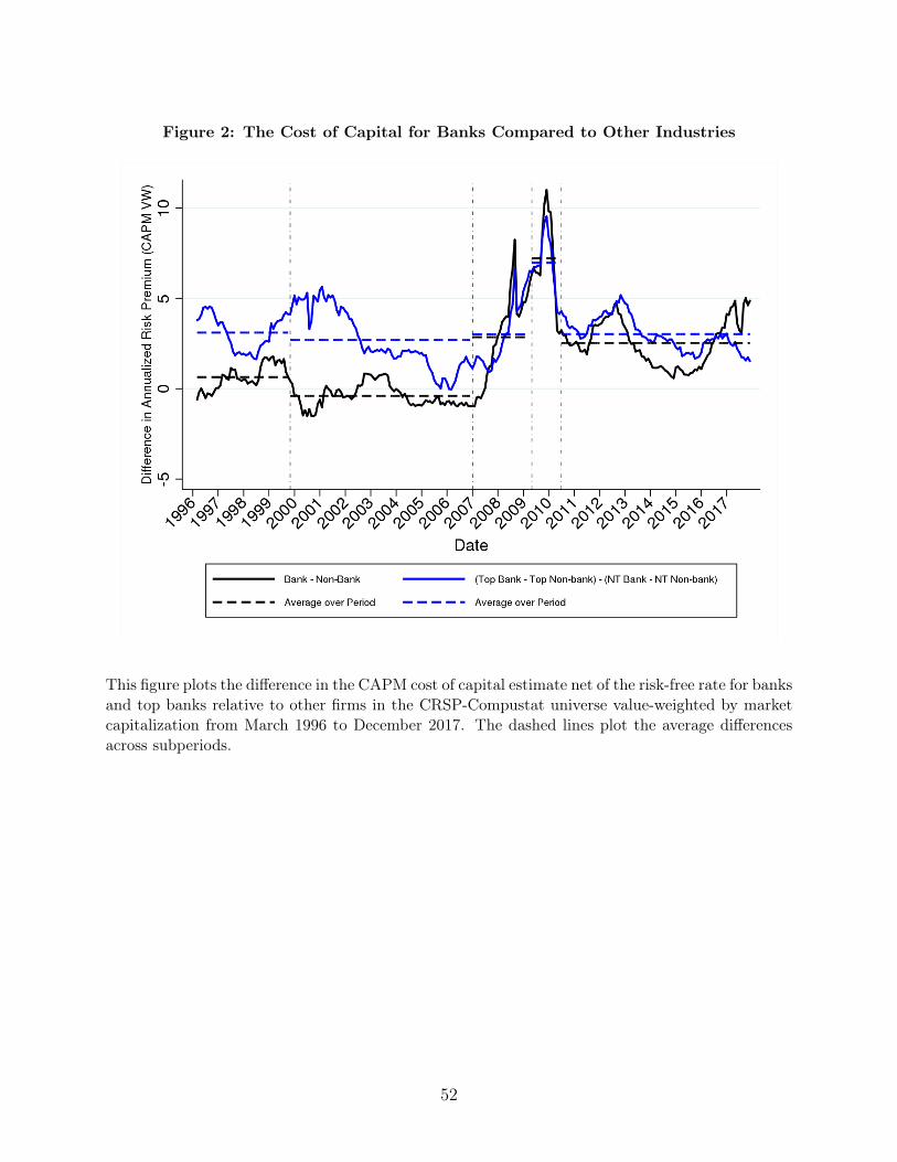
Figure 2: The Cost of Capital for Banks Compared to Other Industries

This figure plots the difference in the CAPM cost of capital estimate net of the risk-free rate for banksand top banks relative to other firms in the CRSP-Compustat universe value-weighted by marketcapitalization from March 1996 to December 2017. The dashed lines plot the average differencesacross subperiods.

52

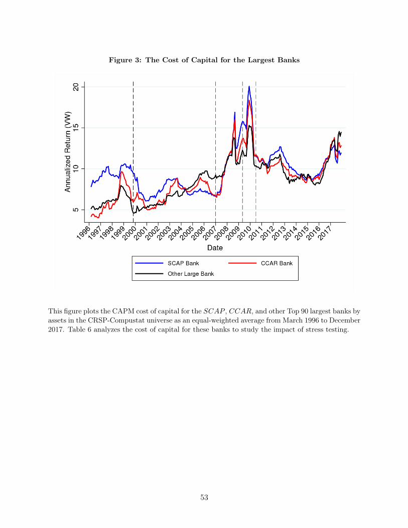
Figure 3: The Cost of Capital for the Largest Banks

This figure plots the CAPM cost of capital for the SCAP , CCAR, and other Top 90 largest banks byassets in the CRSP-Compustat universe as an equal-weighted average from March 1996 to December2017. Table 6 analyzes the cost of capital for these banks to study the impact of stress testing.

53

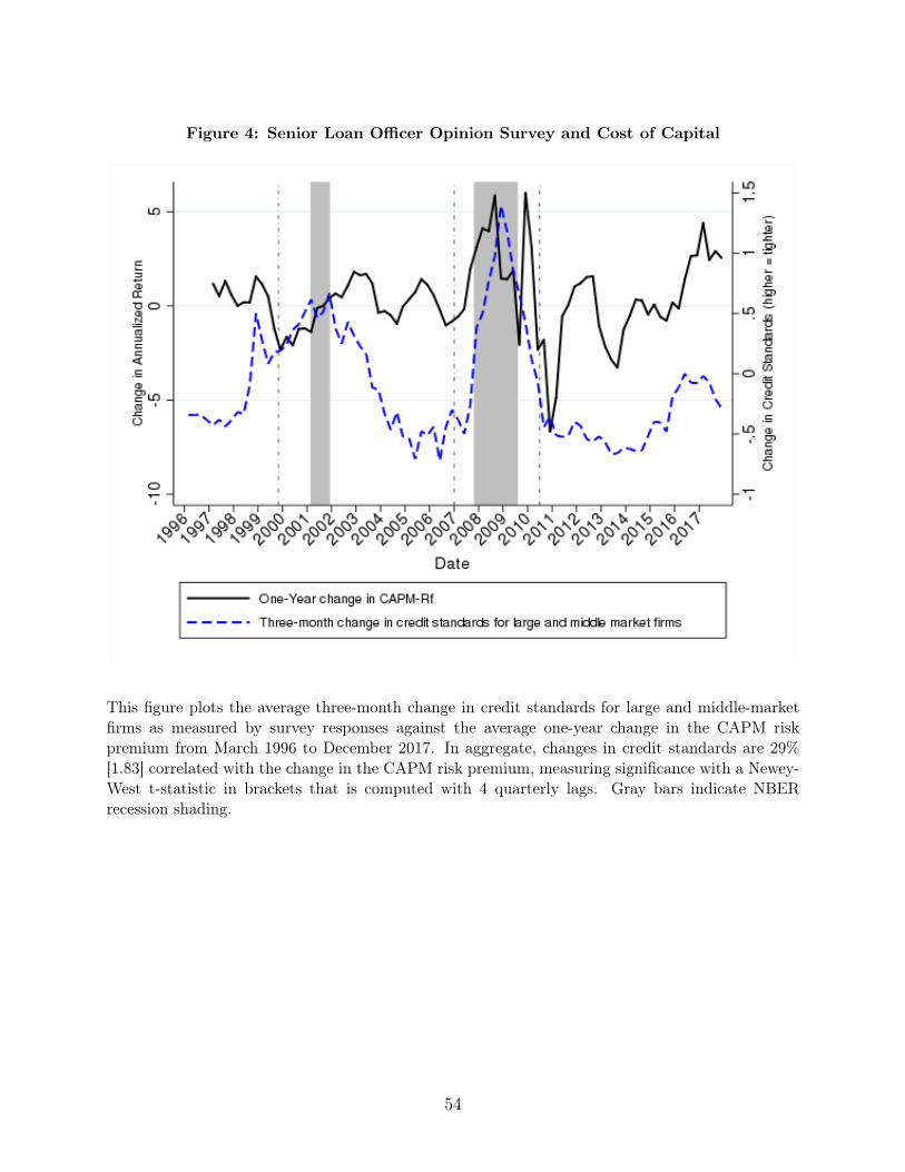
Figure 4: Senior Loan Officer Opinion Survey and Cost of Capital

This figure plots the average three-month change in credit standards for large and middle-marketfirms as measured by survey responses against the average one-year change in the CAPM riskpremium from March 1996 to December 2017. In aggregate, changes in credit standards are 29%[1.83] correlated with the change in the CAPM risk premium, measuring significance with a Newey-West t-statistic in brackets that is computed with 4 quarterly lags. Gray bars indicate NBERrecession shading.

54

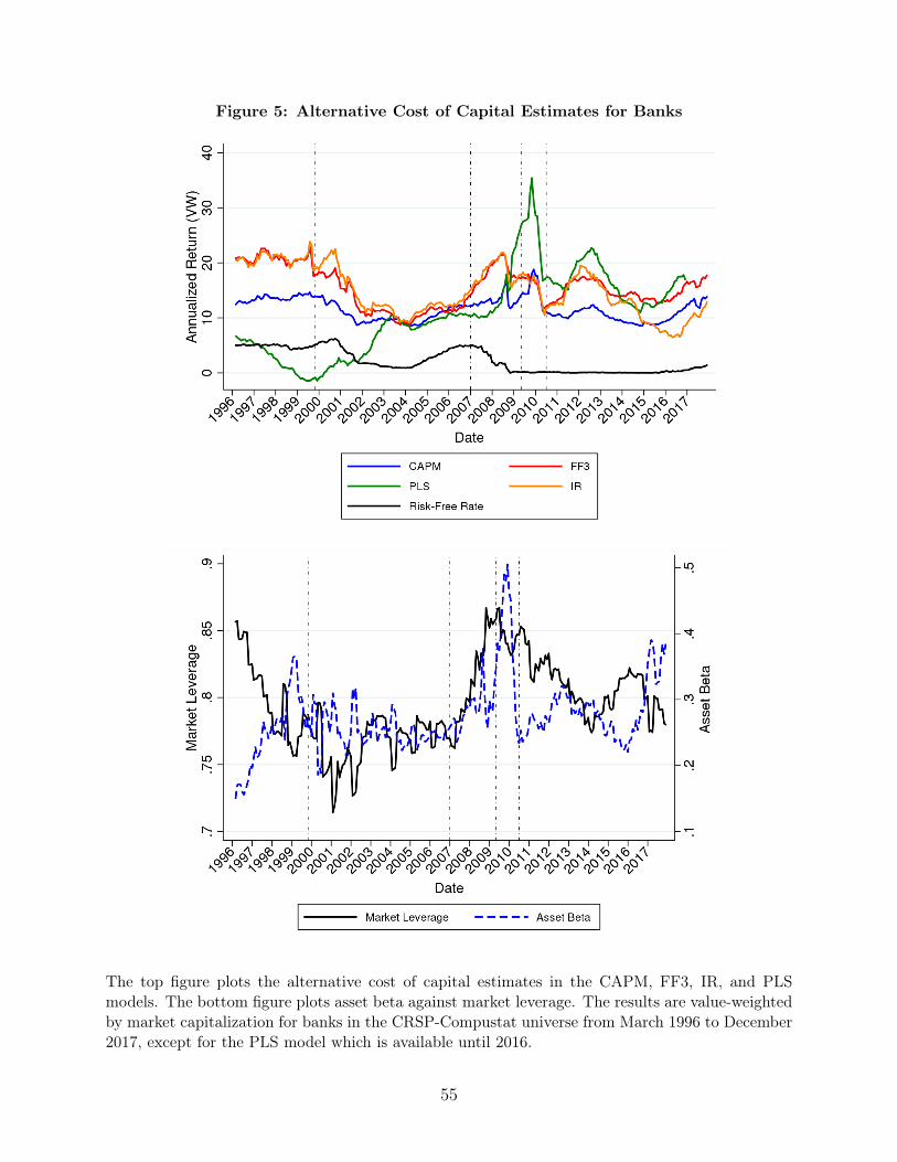
Figure 5: Alternative Cost of Capital Estimates for Banks

The top figure plots the alternative cost of capital estimates in the CAPM, FF3, IR, and PLSmodels. The bottom figure plots asset beta against market leverage. The results are value-weightedby market capitalization for banks in the CRSP-Compustat universe from March 1996 to December2017, except for the PLS model which is available until 2016.

55

A Appendix

A.1 Alternative definitions of regulatory breaks

In addition to varying our regulatory time periods by a few months, we experiment withdifferent time series breaks. Because the SCAP was a one time stress test rather than aregulatory change, Table A.1 reports the results combining the Crisis and SCAP periods intoa single Crisis period. Using these definitions, specifications (2) and (3) indicate that banksdifferential cost of capital declined by approximately 150 basis points from the combinedCrisis period to the Dodd-Frank period, a result that remains economically and statisticallysignificant. In comparison, specifications (2) and (3) in Table 3 feature a significant declineof 450 basis points from SCAP to Dodd-Frank for banks but an insignificant decline from theCrisis to Dodd-Frank. Taken together these results reflect how banks CAPM betas increasedsignificantly during the SCAP period from May 2009 to June 2010. This timing is in parta feature of our estimation approach that uses rolling one-year regressions with lagged datato estimate betas, indicating that bank betas were increasing the most during the fall ofthe financial crisis and in the ensuing months. Similarly, there continues to be a differentialdecline in the cost of capital for the very largest banks from the combined Crisis period toDodd-Frank but with a smaller magnitude than before.

A.2 Alternative bank sample

To understand the robustness of our results to the definition of banks, Table A.2 reportsthe main difference-in-differences regressions defining banks as those firms whose two-digitSIC code is 60 (depository institutions). These regressions drop firms that were previouslyidentified as banks but had SIC codes that did not begin with 60, since these firms arealso subject to changes in bank regulation and thus do not belong in the comparison group.Results are generally similar to those presented in the paper, suggesting that the results arenot sensitive to the definition of banks and that the changes to banks’ cost of capital are notbeing driven solely by changes to the sample of regulated banks.

A.3 Alternative beta estimation methods

In addition to exploring alternative factor models to the CAPM, we also check the robustnessof our findings by varying the estimation method for computing time-varying betas. TableA.3 summarizes these results by reporting value-weighted difference-in-difference regressionsfor the CAPM, three-factor, and five-factor models using different estimation methods to

56

compute the betas for each of these models. In unreported analysis we confirm that similarresults hold for specifications that include firm fixed effects.

Overall we find that the cost of capital estimates are similar across the different betaestimation methods. In the first column (1) we report the baseline approach in which laggedbetas are estimated from rolling regressions using daily returns over a one-year window. Thesecond column (2) repeats this analysis using rolling regressions with overlapping weeklyreturns instead of daily returns. The third column (3) follows Ang and Kristensen (2012) toestimate centered betas from rolling Gaussian kernel-weighted regressions with an optimalbandwidth parameter that is selected for daily returns. The fourth column (4) estimateslagged betas following the betting-against-beta approach from Frazzini and Pedersen (2014)for the CAPM.

Comparing the betas estimated from daily versus weekly returns, the betas from dailyreturns should be preferred in the absence of microstructure noise as the accuracy of co-variance estimation is increasing in the sampling frequency (Merton 1980). However, inthe presence of noise such as nonsynchronous observations of firm-level and factor returns,zooming out to a lower frequency may be preferred. Empirically, we find the results aresimilar using betas estimated from daily and weekly returns. For example, the CAPM riskpremium declines by 4.67% using daily betas and 4.07% using weekly betas from the SCAPto the Dodd-Frank period while increasing 1.89% and 1.32% relative to the pre-GLB period.The standard errors on these coefficients are about .50% to 1%, so these differences are notstatistically significant. There is a difference, however, for the weekly beta estimates in theSCAP period where banks cost of capital appears somewhat lower in column (2) relative tocolumn (1). In this case, one might argue in favor of the daily betas on economic grounds, asweekly returns during the financial crisis may be smoothing over some of the volatile movesin bank stocks that were correlated with the risk factors at daily and higher frequencies.

In column (3) the Ang and Kristensen (2012) estimates (AK) differ from the other mea-sures as they reflect centered betas that are smoothed in Gaussian kernel-weighted regres-sions.19 Despite these differences, the results are relatively similar across the different models.For example, in the case of the CAPM, the AK risk premium declined by 2.65% from SCAPto Dodd-Frank. While this magnitude is somewhat lower than in columns (1) and (2), the

19The optimal bandwidth balances the bias-variance trade-off in estimating the time-varying betas. Itis estimated from a first-stage regression using a uniform one-sided kernel with 252 days of lagged data(the baseline estimates). The distribution of optimal bandwidths for the second-stage regressions has a 1.96z-score for the Gaussian kernel at .47, .88, 1.01, 1.12, and 1.48 years for the 1st, 25th, 50th, 75th, and 99thquantiles respectively. As a result, most of the weight for the kernel regressions falls within one-year of thecurrent date. In rare cases where the 1.96 z-score is less than 3-months, we truncate the optimal bandwidthto ensure that at least 6-monthns of data fall within 95% of the mass for the Gaussian kernel. The truncationimpacts less than .01% of observations.

57

AK estimates also feature a higher cost of capital for banks in the Crisis period relativeto the daily and weekly betas. The CAPM risk premium for banks increases by 3.5% incolumn (3) versus only 1.87% and .90% increases in columns (1) and (2). Taken together,these differences reflect how the centered AK betas have shifted and smoothed some of thedifferential increase in the cost of capital for banks.

Finally, in column (4), the betting-against-beta approach separates the estimation ofthe firm-level volatility and correlation parameters for the CAPM. Following Frazzini andPedersen (2014), volatility is estimated using daily log-returns over the past year whilecorrelation with the market is estimated using three-day log returns over the past five years.The results are similar to the estimates in columns (1) and (2), with the different treatment ofthe volatility and correlation parameters reflecting the tradeoffs in using daily versus weeklydata as discussed above.

A.4 Additional Time-Varying Bank Characteristic Analysis

RWA is a complicated metric which makes it difficult to interpret the change in the bankx time interaction coefficients between column (2) and column (7) in Table 5. Table A.4extends the analysis by decomposing RWA into its component parts to better understandwhich type of risks are driving changes in the cost of capital over time. We examine therelationship between the cost of capital and securities (including cash, available-for-saleand held-to-maturity securities, and securities purchased under agreements to resell), loans,trading assets, loan commitments, and total derivatives. As before, we first include all ofthe variables unconditionally, then one by one conditionally, and then all conditionally withtime-varying coefficients. While none of the RWA components by itself reverses the generalpatterns, we do find, as in Table 5 specification (7), that including all RWA componentsresults in no significant change for banks’ cost of capital from the SCAP to the Dodd-Frankperiods. In addition, from inspecting the coefficients for the different components, we findevidence that loans and loan commitments drive part of the increase in RWA’s explanatorypower during the SCAP period, although not enough to explain all of the change in banks’cost of capital following the financial crisis. This contrasts securities, trading, and derivativeswhose coefficients are roughly stable since the GLB period. Finally, we extend the analysisfrom Table 5 for the largest banks by adding the bank x Top interaction terms. In theseregressions we find a decline in the largest banks’ cost of capital by about 3% to 4% from theSCAP to the Dodd-Frank period across specifications, even with the increased coefficient onRWA during the SCAP period in specification (7). This indicates that RWA is not drivingthe results for the very largest banks, a result that contrasts Tables 5 and A.4.

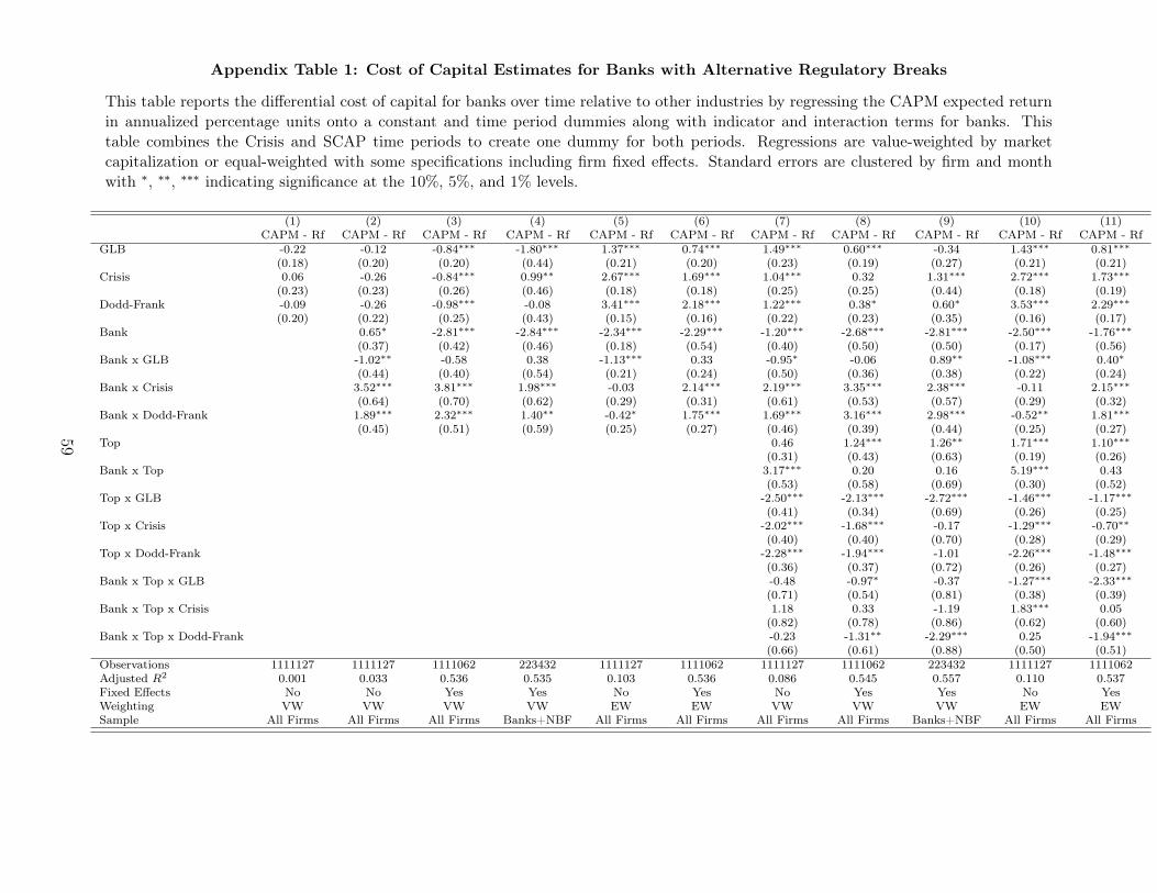
Appendix Table 1: Cost of Capital Estimates for Banks with Alternative Regulatory Breaks

This table reports the differential cost of capital for banks over time relative to other industries by regressing the CAPM expected returnin annualized percentage units onto a constant and time period dummies along with indicator and interaction terms for banks. Thistable combines the Crisis and SCAP time periods to create one dummy for both periods. Regressions are value-weighted by marketcapitalization or equal-weighted with some specifications including firm fixed effects. Standard errors are clustered by firm and monthwith ∗, ∗∗, ∗∗∗ indicating significance at the 10%, 5%, and 1% levels.

(1) (2) (3) (4) (5) (6) (7) (8) (9) (10) (11)CAPM - Rf CAPM - Rf CAPM - Rf CAPM - Rf CAPM - Rf CAPM - Rf CAPM - Rf CAPM - Rf CAPM - Rf CAPM - Rf CAPM - Rf

GLB -0.22 -0.12 -0.84∗∗∗ -1.80∗∗∗ 1.37∗∗∗ 0.74∗∗∗ 1.49∗∗∗ 0.60∗∗∗ -0.34 1.43∗∗∗ 0.81∗∗∗(0.18) (0.20) (0.20) (0.44) (0.21) (0.20) (0.23) (0.19) (0.27) (0.21) (0.21)

Crisis 0.06 -0.26 -0.84∗∗∗ 0.99∗∗ 2.67∗∗∗ 1.69∗∗∗ 1.04∗∗∗ 0.32 1.31∗∗∗ 2.72∗∗∗ 1.73∗∗∗(0.23) (0.23) (0.26) (0.46) (0.18) (0.18) (0.25) (0.25) (0.44) (0.18) (0.19)

Dodd-Frank -0.09 -0.26 -0.98∗∗∗ -0.08 3.41∗∗∗ 2.18∗∗∗ 1.22∗∗∗ 0.38∗ 0.60∗ 3.53∗∗∗ 2.29∗∗∗(0.20) (0.22) (0.25) (0.43) (0.15) (0.16) (0.22) (0.23) (0.35) (0.16) (0.17)

Bank 0.65∗ -2.81∗∗∗ -2.84∗∗∗ -2.34∗∗∗ -2.29∗∗∗ -1.20∗∗∗ -2.68∗∗∗ -2.81∗∗∗ -2.50∗∗∗ -1.76∗∗∗(0.37) (0.42) (0.46) (0.18) (0.54) (0.40) (0.50) (0.50) (0.17) (0.56)

Bank x GLB -1.02∗∗ -0.58 0.38 -1.13∗∗∗ 0.33 -0.95∗ -0.06 0.89∗∗ -1.08∗∗∗ 0.40∗(0.44) (0.40) (0.54) (0.21) (0.24) (0.50) (0.36) (0.38) (0.22) (0.24)

Bank x Crisis 3.52∗∗∗ 3.81∗∗∗ 1.98∗∗∗ -0.03 2.14∗∗∗ 2.19∗∗∗ 3.35∗∗∗ 2.38∗∗∗ -0.11 2.15∗∗∗(0.64) (0.70) (0.62) (0.29) (0.31) (0.61) (0.53) (0.57) (0.29) (0.32)

Bank x Dodd-Frank 1.89∗∗∗ 2.32∗∗∗ 1.40∗∗ -0.42∗ 1.75∗∗∗ 1.69∗∗∗ 3.16∗∗∗ 2.98∗∗∗ -0.52∗∗ 1.81∗∗∗(0.45) (0.51) (0.59) (0.25) (0.27) (0.46) (0.39) (0.44) (0.25) (0.27)

Top 0.46 1.24∗∗∗ 1.26∗∗ 1.71∗∗∗ 1.10∗∗∗(0.31) (0.43) (0.63) (0.19) (0.26)

Bank x Top 3.17∗∗∗ 0.20 0.16 5.19∗∗∗ 0.43(0.53) (0.58) (0.69) (0.30) (0.52)

Top x GLB -2.50∗∗∗ -2.13∗∗∗ -2.72∗∗∗ -1.46∗∗∗ -1.17∗∗∗(0.41) (0.34) (0.69) (0.26) (0.25)

Top x Crisis -2.02∗∗∗ -1.68∗∗∗ -0.17 -1.29∗∗∗ -0.70∗∗(0.40) (0.40) (0.70) (0.28) (0.29)

Top x Dodd-Frank -2.28∗∗∗ -1.94∗∗∗ -1.01 -2.26∗∗∗ -1.48∗∗∗(0.36) (0.37) (0.72) (0.26) (0.27)

Bank x Top x GLB -0.48 -0.97∗ -0.37 -1.27∗∗∗ -2.33∗∗∗(0.71) (0.54) (0.81) (0.38) (0.39)

Bank x Top x Crisis 1.18 0.33 -1.19 1.83∗∗∗ 0.05(0.82) (0.78) (0.86) (0.62) (0.60)

Bank x Top x Dodd-Frank -0.23 -1.31∗∗ -2.29∗∗∗ 0.25 -1.94∗∗∗(0.66) (0.61) (0.88) (0.50) (0.51)

Observations 1111127 1111127 1111062 223432 1111127 1111062 1111127 1111062 223432 1111127 1111062Adjusted R2 0.001 0.033 0.536 0.535 0.103 0.536 0.086 0.545 0.557 0.110 0.537Fixed Effects No No Yes Yes No Yes No Yes Yes No YesWeighting VW VW VW VW EW EW VW VW VW EW EWSample All Firms All Firms All Firms Banks+NBF All Firms All Firms All Firms All Firms Banks+NBF All Firms All Firms

59

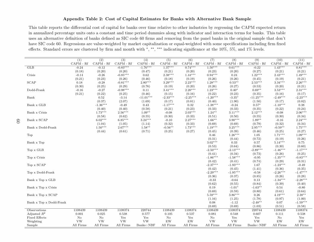
Appendix Table 2: Cost of Capital Estimates for Banks with Alternative Bank Sample

This table reports the differential cost of capital for banks over time relative to other industries by regressing the CAPM expected returnin annualized percentage units onto a constant and time period dummies along with indicator and interaction terms for banks. This tableuses an alternative definition of banks defined as SIC code 60 firms and removing from the panel banks in the original sample that don’thave SIC code 60. Regressions are value-weighted by market capitalization or equal-weighted with some specifications including firm fixedeffects. Standard errors are clustered by firm and month with ∗, ∗∗, ∗∗∗ indicating significance at the 10%, 5%, and 1% levels.

(1) (2) (3) (4) (5) (6) (7) (8) (9) (10) (11)CAPM - Rf CAPM - Rf CAPM - Rf CAPM - Rf CAPM - Rf CAPM - Rf CAPM - Rf CAPM - Rf CAPM - Rf CAPM - Rf CAPM - Rf

GLB -0.24 -0.12 -0.83∗∗∗ -1.76∗∗∗ 1.37∗∗∗ 0.74∗∗∗ 1.50∗∗∗ 0.61∗∗∗ -0.22 1.43∗∗∗ 0.81∗∗∗(0.18) (0.20) (0.20) (0.47) (0.21) (0.20) (0.23) (0.20) (0.27) (0.21) (0.21)

Crisis -0.14 -0.26 -0.85∗∗∗ 0.62 2.38∗∗∗ 1.44∗∗∗ 0.94∗∗∗ 0.24 1.22∗∗∗ 2.43∗∗∗ 1.49∗∗∗(0.21) (0.23) (0.26) (0.46) (0.18) (0.19) (0.26) (0.26) (0.45) (0.19) (0.21)

SCAP 0.18 -0.28 -0.81∗∗∗ 2.80∗∗∗ 3.29∗∗∗ 2.23∗∗∗ 1.28∗∗∗ 0.53∗∗ 2.53∗∗∗ 3.34∗∗∗ 2.26∗∗∗(0.30) (0.25) (0.29) (0.76) (0.19) (0.20) (0.26) (0.27) (0.53) (0.20) (0.21)

Dodd-Frank -0.16 -0.27 -0.98∗∗∗ 0.11 3.41∗∗∗ 2.20∗∗∗ 1.23∗∗∗ 0.40∗ 0.69∗∗ 3.53∗∗∗ 2.31∗∗∗(0.21) (0.22) (0.25) (0.46) (0.15) (0.16) (0.22) (0.23) (0.35) (0.16) (0.17)

Bank 0.52 -3.14 -11.01∗∗∗ -2.33∗∗∗ -2.25∗∗∗ -1.20∗∗∗ -3.35∗ -11.25∗∗∗ -2.49∗∗∗ -2.23∗∗∗(0.37) (2.07) (1.69) (0.17) (0.81) (0.40) (1.90) (1.50) (0.17) (0.82)

Bank x GLB -1.36∗∗∗ -0.49 0.43 -1.17∗∗∗ 0.32 -1.38∗∗∗ -0.24 0.57∗ -1.10∗∗∗ 0.38(0.40) (0.40) (0.58) (0.21) (0.23) (0.33) (0.33) (0.35) (0.22) (0.24)

Bank x Crisis 1.73∗∗∗ 2.56∗∗∗ 1.09∗∗ -0.08 2.03∗∗∗ 1.24∗∗ 3.11∗∗∗ 2.12∗∗∗ -0.08 2.06∗∗∗(0.58) (0.62) (0.55) (0.30) (0.33) (0.51) (0.50) (0.55) (0.30) (0.34)

Bank x SCAP 6.02∗∗∗ 6.85∗∗∗ 3.24∗∗∗ -0.10 2.27∗∗∗ 1.66∗∗ 3.90∗∗∗ 1.89∗∗ -0.16 2.24∗∗∗(1.04) (1.05) (1.14) (0.32) (0.33) (0.69) (0.69) (0.79) (0.32) (0.34)

Bank x Dodd-Frank 1.50∗∗∗ 2.67∗∗∗ 1.58∗∗ -0.56∗∗ 1.73∗∗∗ 1.19∗∗∗ 3.25∗∗∗ 2.95∗∗∗ -0.59∗∗ 1.75∗∗∗(0.44) (0.61) (0.71) (0.25) (0.27) (0.45) (0.39) (0.46) (0.25) (0.27)

Top 0.46 1.26∗∗∗ 1.05 1.71∗∗∗ 1.09∗∗∗(0.31) (0.44) (0.72) (0.19) (0.26)

Bank x Top 3.02∗∗∗ 0.33 0.57 5.14∗∗∗ 0.75(0.53) (0.64) (0.86) (0.30) (0.60)

Top x GLB -2.50∗∗∗ -2.13∗∗∗ -2.89∗∗∗ -1.46∗∗∗ -1.17∗∗∗(0.41) (0.34) (0.73) (0.26) (0.25)

Top x Crisis -1.86∗∗∗ -1.58∗∗∗ -0.95 -1.35∗∗∗ -0.83∗∗∗(0.42) (0.41) (0.74) (0.29) (0.31)

Top x SCAP -2.37∗∗∗ -1.93∗∗∗ 1.67 -1.23∗∗∗ -0.49(0.42) (0.45) (1.41) (0.36) (0.35)

Top x Dodd-Frank -2.29∗∗∗ -1.95∗∗∗ -0.58 -2.26∗∗∗ -1.47∗∗∗(0.36) (0.37) (0.85) (0.26) (0.28)

Bank x Top x GLB -0.33 -0.64 0.13 -1.34∗∗∗ -2.28∗∗∗(0.62) (0.55) (0.84) (0.39) (0.40)

Bank x Top x Crisis 0.19 -1.01∗ -1.63∗∗ 0.54 -0.80(0.69) (0.59) (0.80) (0.61) (0.64)

Bank x Top x SCAP 5.59∗∗∗ 3.86∗∗∗ 0.26 4.19∗∗∗ 2.38∗∗(1.16) (1.25) (1.78) (0.97) (1.00)

Bank x Top x Dodd-Frank 0.08 -1.12 -2.48∗∗ 0.07 -1.59∗∗∗(0.69) (0.69) (1.03) (0.51) (0.58)

Observations 1108439 1108439 1108374 220744 1108439 1108374 1108439 1108374 220744 1108439 1108374Adjusted R2 0.001 0.025 0.538 0.577 0.105 0.537 0.081 0.548 0.607 0.111 0.538Fixed Effects No No Yes Yes No Yes No Yes Yes No YesWeighting VW VW VW VW EW EW VW VW VW EW EWSample All Firms All Firms All Firms Banks+NBF All Firms All Firms All Firms All Firms Banks+NBF All Firms All Firms

60

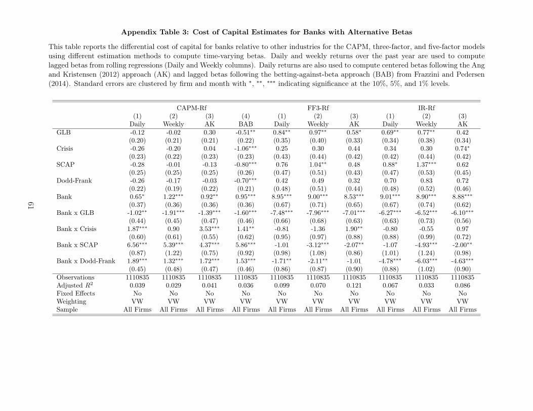
Appendix Table 3: Cost of Capital Estimates for Banks with Alternative Betas

This table reports the differential cost of capital for banks relative to other industries for the CAPM, three-factor, and five-factor modelsusing different estimation methods to compute time-varying betas. Daily and weekly returns over the past year are used to computelagged betas from rolling regressions (Daily and Weekly columns). Daily returns are also used to compute centered betas following the Angand Kristensen (2012) approach (AK) and lagged betas following the betting-against-beta approach (BAB) from Frazzini and Pedersen(2014). Standard errors are clustered by firm and month with ∗, ∗∗, ∗∗∗ indicating significance at the 10%, 5%, and 1% levels.

CAPM-Rf FF3-Rf IR-Rf(1) (2) (3) (4) (1) (2) (3) (1) (2) (3)

Daily Weekly AK BAB Daily Weekly AK Daily Weekly AKGLB -0.12 -0.02 0.30 -0.51∗∗ 0.84∗∗ 0.97∗∗ 0.58∗ 0.69∗∗ 0.77∗∗ 0.42

(0.20) (0.21) (0.21) (0.22) (0.35) (0.40) (0.33) (0.34) (0.38) (0.34)Crisis -0.26 -0.20 0.04 -1.06∗∗∗ 0.25 0.30 0.44 0.34 0.30 0.74∗

(0.23) (0.22) (0.23) (0.23) (0.43) (0.44) (0.42) (0.42) (0.44) (0.42)SCAP -0.28 -0.01 -0.13 -0.80∗∗∗ 0.76 1.04∗∗ 0.48 0.88∗ 1.37∗∗∗ 0.62

(0.25) (0.25) (0.25) (0.26) (0.47) (0.51) (0.43) (0.47) (0.53) (0.45)Dodd-Frank -0.26 -0.17 -0.03 -0.70∗∗∗ 0.42 0.49 0.32 0.70 0.83 0.72

(0.22) (0.19) (0.22) (0.21) (0.48) (0.51) (0.44) (0.48) (0.52) (0.46)Bank 0.65∗ 1.22∗∗∗ 0.92∗∗ 0.95∗∗∗ 8.95∗∗∗ 9.00∗∗∗ 8.53∗∗∗ 9.01∗∗∗ 8.90∗∗∗ 8.88∗∗∗

(0.37) (0.36) (0.36) (0.36) (0.67) (0.71) (0.65) (0.67) (0.74) (0.62)Bank x GLB -1.02∗∗ -1.91∗∗∗ -1.39∗∗∗ -1.60∗∗∗ -7.48∗∗∗ -7.96∗∗∗ -7.01∗∗∗ -6.27∗∗∗ -6.52∗∗∗ -6.10∗∗∗

(0.44) (0.45) (0.47) (0.46) (0.66) (0.68) (0.63) (0.63) (0.73) (0.56)Bank x Crisis 1.87∗∗∗ 0.90 3.53∗∗∗ 1.41∗∗ -0.81 -1.36 1.90∗∗ -0.80 -0.55 0.97

(0.60) (0.61) (0.55) (0.62) (0.95) (0.97) (0.88) (0.88) (0.99) (0.72)Bank x SCAP 6.56∗∗∗ 5.39∗∗∗ 4.37∗∗∗ 5.86∗∗∗ -1.01 -3.12∗∗∗ -2.07∗∗ -1.07 -4.93∗∗∗ -2.00∗∗

(0.87) (1.22) (0.75) (0.92) (0.98) (1.08) (0.86) (1.01) (1.24) (0.98)Bank x Dodd-Frank 1.89∗∗∗ 1.32∗∗∗ 1.72∗∗∗ 1.53∗∗∗ -1.71∗∗ -2.11∗∗ -1.01 -4.78∗∗∗ -6.03∗∗∗ -4.63∗∗∗

(0.45) (0.48) (0.47) (0.46) (0.86) (0.87) (0.90) (0.88) (1.02) (0.90)Observations 1110835 1110835 1110835 1110835 1110835 1110835 1110835 1110835 1110835 1110835Adjusted R2 0.039 0.029 0.041 0.036 0.099 0.070 0.121 0.067 0.033 0.086Fixed Effects No No No No No No No No No NoWeighting VW VW VW VW VW VW VW VW VW VWSample All Firms All Firms All Firms All Firms All Firms All Firms All Firms All Firms All Firms All Firms

61

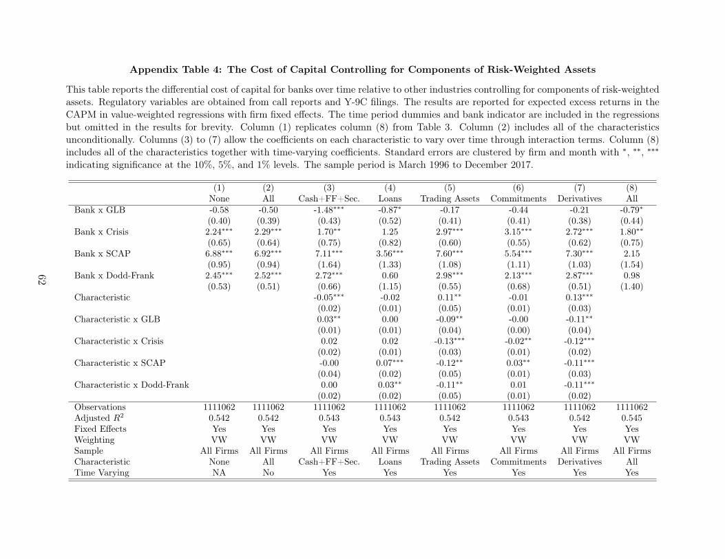
Appendix Table 4: The Cost of Capital Controlling for Components of Risk-Weighted Assets

This table reports the differential cost of capital for banks over time relative to other industries controlling for components of risk-weightedassets. Regulatory variables are obtained from call reports and Y-9C filings. The results are reported for expected excess returns in theCAPM in value-weighted regressions with firm fixed effects. The time period dummies and bank indicator are included in the regressionsbut omitted in the results for brevity. Column (1) replicates column (8) from Table 3. Column (2) includes all of the characteristicsunconditionally. Columns (3) to (7) allow the coefficients on each characteristic to vary over time through interaction terms. Column (8)includes all of the characteristics together with time-varying coefficients. Standard errors are clustered by firm and month with ∗, ∗∗, ∗∗∗

indicating significance at the 10%, 5%, and 1% levels. The sample period is March 1996 to December 2017.

(1) (2) (3) (4) (5) (6) (7) (8)None All Cash+FF+Sec. Loans Trading Assets Commitments Derivatives All

Bank x GLB -0.58 -0.50 -1.48∗∗∗ -0.87∗ -0.17 -0.44 -0.21 -0.79∗(0.40) (0.39) (0.43) (0.52) (0.41) (0.41) (0.38) (0.44)

Bank x Crisis 2.24∗∗∗ 2.29∗∗∗ 1.70∗∗ 1.25 2.97∗∗∗ 3.15∗∗∗ 2.72∗∗∗ 1.80∗∗(0.65) (0.64) (0.75) (0.82) (0.60) (0.55) (0.62) (0.75)

Bank x SCAP 6.88∗∗∗ 6.92∗∗∗ 7.11∗∗∗ 3.56∗∗∗ 7.60∗∗∗ 5.54∗∗∗ 7.30∗∗∗ 2.15(0.95) (0.94) (1.64) (1.33) (1.08) (1.11) (1.03) (1.54)

Bank x Dodd-Frank 2.45∗∗∗ 2.52∗∗∗ 2.72∗∗∗ 0.60 2.98∗∗∗ 2.13∗∗∗ 2.87∗∗∗ 0.98(0.53) (0.51) (0.66) (1.15) (0.55) (0.68) (0.51) (1.40)

Characteristic -0.05∗∗∗ -0.02 0.11∗∗ -0.01 0.13∗∗∗(0.02) (0.01) (0.05) (0.01) (0.03)

Characteristic x GLB 0.03∗∗ 0.00 -0.09∗∗ -0.00 -0.11∗∗(0.01) (0.01) (0.04) (0.00) (0.04)

Characteristic x Crisis 0.02 0.02 -0.13∗∗∗ -0.02∗∗ -0.12∗∗∗(0.02) (0.01) (0.03) (0.01) (0.02)

Characteristic x SCAP -0.00 0.07∗∗∗ -0.12∗∗ 0.03∗∗ -0.11∗∗∗(0.04) (0.02) (0.05) (0.01) (0.03)

Characteristic x Dodd-Frank 0.00 0.03∗∗ -0.11∗∗ 0.01 -0.11∗∗∗(0.02) (0.02) (0.05) (0.01) (0.02)

Observations 1111062 1111062 1111062 1111062 1111062 1111062 1111062 1111062Adjusted R2 0.542 0.542 0.543 0.543 0.542 0.543 0.542 0.545Fixed Effects Yes Yes Yes Yes Yes Yes Yes YesWeighting VW VW VW VW VW VW VW VWSample All Firms All Firms All Firms All Firms All Firms All Firms All Firms All FirmsCharacteristic None All Cash+FF+Sec. Loans Trading Assets Commitments Derivatives AllTime Varying NA No Yes Yes Yes Yes Yes Yes

62

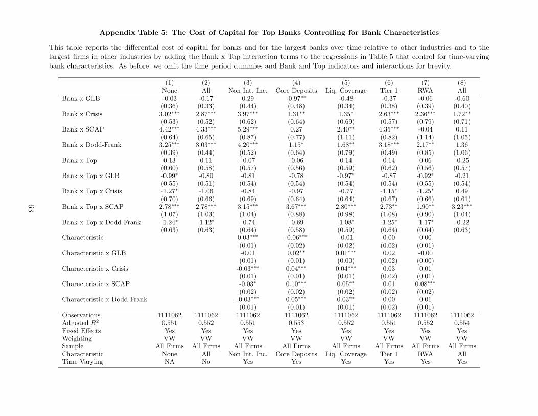
Appendix Table 5: The Cost of Capital for Top Banks Controlling for Bank Characteristics

This table reports the differential cost of capital for banks and for the largest banks over time relative to other industries and to thelargest firms in other industries by adding the Bank x Top interaction terms to the regressions in Table 5 that control for time-varyingbank characteristics. As before, we omit the time period dummies and Bank and Top indicators and interactions for brevity.

(1) (2) (3) (4) (5) (6) (7) (8)None All Non Int. Inc. Core Deposits Liq. Coverage Tier 1 RWA All

Bank x GLB -0.03 -0.17 0.29 -0.97∗∗ -0.48 -0.37 -0.06 -0.60(0.36) (0.33) (0.44) (0.48) (0.34) (0.38) (0.39) (0.40)

Bank x Crisis 3.02∗∗∗ 2.87∗∗∗ 3.97∗∗∗ 1.31∗∗ 1.35∗ 2.63∗∗∗ 2.36∗∗∗ 1.72∗∗(0.53) (0.52) (0.62) (0.64) (0.69) (0.57) (0.79) (0.71)

Bank x SCAP 4.42∗∗∗ 4.33∗∗∗ 5.29∗∗∗ 0.27 2.40∗∗ 4.35∗∗∗ -0.04 0.11(0.64) (0.65) (0.87) (0.77) (1.11) (0.82) (1.14) (1.05)

Bank x Dodd-Frank 3.25∗∗∗ 3.03∗∗∗ 4.20∗∗∗ 1.15∗ 1.68∗∗ 3.18∗∗∗ 2.17∗∗ 1.36(0.39) (0.44) (0.52) (0.64) (0.79) (0.49) (0.85) (1.06)

Bank x Top 0.13 0.11 -0.07 -0.06 0.14 0.14 0.06 -0.25(0.60) (0.58) (0.57) (0.56) (0.59) (0.62) (0.56) (0.57)

Bank x Top x GLB -0.99∗ -0.80 -0.81 -0.78 -0.97∗ -0.87 -0.92∗ -0.21(0.55) (0.51) (0.54) (0.54) (0.54) (0.54) (0.55) (0.54)

Bank x Top x Crisis -1.27∗ -1.06 -0.84 -0.97 -0.77 -1.15∗ -1.25∗ 0.49(0.70) (0.66) (0.69) (0.64) (0.64) (0.67) (0.66) (0.61)

Bank x Top x SCAP 2.78∗∗∗ 2.78∗∗∗ 3.15∗∗∗ 3.67∗∗∗ 2.80∗∗∗ 2.73∗∗ 1.90∗∗ 3.23∗∗∗(1.07) (1.03) (1.04) (0.88) (0.98) (1.08) (0.90) (1.04)

Bank x Top x Dodd-Frank -1.24∗ -1.12∗ -0.74 -0.69 -1.08∗ -1.25∗ -1.17∗ -0.22(0.63) (0.63) (0.64) (0.58) (0.59) (0.64) (0.64) (0.63)

Characteristic 0.03∗∗∗ -0.06∗∗∗ -0.01 0.00 0.00(0.01) (0.02) (0.02) (0.02) (0.01)

Characteristic x GLB -0.01 0.02∗∗ 0.01∗∗∗ 0.02 -0.00(0.01) (0.01) (0.00) (0.02) (0.00)

Characteristic x Crisis -0.03∗∗∗ 0.04∗∗∗ 0.04∗∗∗ 0.03 0.01(0.01) (0.01) (0.01) (0.02) (0.01)

Characteristic x SCAP -0.03∗ 0.10∗∗∗ 0.05∗∗ 0.01 0.08∗∗∗(0.02) (0.02) (0.02) (0.02) (0.02)

Characteristic x Dodd-Frank -0.03∗∗∗ 0.05∗∗∗ 0.03∗∗ 0.00 0.01(0.01) (0.01) (0.01) (0.02) (0.01)

Observations 1111062 1111062 1111062 1111062 1111062 1111062 1111062 1111062Adjusted R2 0.551 0.552 0.551 0.553 0.552 0.551 0.552 0.554Fixed Effects Yes Yes Yes Yes Yes Yes Yes YesWeighting VW VW VW VW VW VW VW VWSample All Firms All Firms All Firms All Firms All Firms All Firms All Firms All FirmsCharacteristic None All Non Int. Inc. Core Deposits Liq. Coverage Tier 1 RWA AllTime Varying NA No Yes Yes Yes Yes Yes Yes

63