Balancing the load in LTE urban networks via inter- frequency handovers José Miguel Querido Guita Thesis to obtain the Master of Science Degree in Electrical and Computer Engineering Supervisor: Prof. Luís Manuel de Jesus Sousa Correia Examination Committee Chairperson: Prof. José Eduardo Charters Ribeiro da Cunha Sanguino Supervisor: Prof. Luís Manuel de Jesus Sousa Correia Members of Committee: Prof. António José Castelo Branco Rodrigues : Eng. Marco Serrazina November 2016

Welcome message from author
This document is posted to help you gain knowledge. Please leave a comment to let me know what you think about it! Share it to your friends and learn new things together.
Transcript
Balancing the load in LTE urban networks via inter-
frequency handovers
José Miguel Querido Guita
Thesis to obtain the Master of Science Degree in
Electrical and Computer Engineering
Supervisor: Prof. Luís Manuel de Jesus Sousa Correia
Examination Committee
Chairperson: Prof. José Eduardo Charters Ribeiro da Cunha Sanguino
Supervisor: Prof. Luís Manuel de Jesus Sousa Correia
Members of Committee: Prof. António José Castelo Branco Rodrigues
: Eng. Marco Serrazina
November 2016

ii

iii
To my family and friends
“Gaining knowledge is the first step to wisdom. Sharing it is the first step to humanity.”
- Unknown

iv

v
Acknowledgements
Acknowledgements
First of all, I want to thank the supervisor of this thesis, Professor Luis M. Correia for giving me the
opportunity of developing a master thesis in collaboration with one of the most important network
operators in Portugal. Instead of just fulfilling his professor role, Luis Correia taught me on how to shape
my work ethics and attitudes, contributing with his advices and professionalism. Also, I want to thank
him for the opportunity of working along with the GROW team, which gave me more knowledge about
a few telecommunications topics that will be a part of future wireless communications.
Special acknowledgements are also dedicated to Eng. Marco Serrazina and Eng. Pedro Lourenço, from
Vodafone, who provided me constructive critics, suggestions and technical support during the
development of this thesis.
For all the friendship and great leisure times in the development of this work, I would like to thank all
GROW members, especially to Behnam Rouzbehani, Hugo da Silva, Kenan Turbic and Tiago Monteiro.
Also, I would like to thank Ema Catarré and Vera Almeida for the companionship and spirit of
cooperation. It was a pleasure working in an environment like this.
To my colleagues and friends from college times a special thanks to: Iuri Figueiredo, Pedro Figueiredo,
Hugo Café, João Jardim, Francisco Duarte, Pedro Marques, Fernando Ribeiro, André Mateus, José
Calisto, and the rest that are not mentioned here, but that in a way or another contributed to make this
journey of 6 years an unforgettable experience. I would also cheer Ana for all the moments that we
spend together and all the patience that she has to put up with me.
Last but not least, I want to thank my Father, Mother and Brothers for all the unconditional support,
motivational words and for everything that they did for me along this journey, without them, any of this
would had not been possible.

vi
vii
Abstract
Abstract
Mobile traffic is commonly time variant and often unbalanced, consequently, a sudden increase in traffic
within a cell can imbalance the system in such a way that hugely deteriorates network performance. The
main purpose of this thesis is to analyse the impact of balancing the load via inter-frequency handovers
in an LTE heterogeneous urban network. The effect of varying some parameters regarding user density
was studied, as well as combination of different frequency bandwidths and service profile, among others,
addressing the 800, 1 800 and 2 600 MHz bands. A model was developed, and implemented in a
simulation environment, which takes a certain distribution of users into account and makes the allocation
of resources depending on system coverage and available capacity, replicating as close as possible the
behaviour of a real network. The analysis on users’ density supports the view that only makes sense to
apply load balancing methods at a certain load in the system. Results show high standards of QoS,
since, for the same service, users experience similar throughputs within each other. In addition, voice
users never suffer handovers due to load balancing (the assigned priority reduces the probability of drop
calls). The model shows that, depending on network conditions, the gain in throughput can reach up to
8%. The variation of throughput thresholds has more impact on the percentage of users that perform
handovers, and therefore, in the gain of the system.
Keywords
Load Balancing, LTE, Inter-Frequency Handovers, Quality of Service, Heterogeneous Network, Load
Optimisation Handovers, Urban Scenario.
viii
Resumo
O tráfego móvel varia no tempo e é muitas vezes desequilibrado, o que resulta que um súbito aumento
dentro de uma célula, possa desequilibrar o sistema de tal forma que compromete consideravelmente
o desempenho da rede. O objetivo deste trabalho é avaliar o impacto do balanceamento de carga
através de handovers inter-frequência numa rede LTE. Estudou-se o efeito da variação de alguns
parâmetros relativos à densidade de utilizadores, combinação de diferentes larguras de banda, perfis
de serviço, entre outros, através das bandas 800, 1 800 e 2 600 MHz. Para tal, foi desenvolvido um
modelo que, em ambiente de simulação, tem em consideração uma certa distribuição de utilizadores e
realiza a alocação de recursos em função da cobertura e capacidade disponível no sistema, tentando
replicar, tanto quanto possível, o comportamento de uma rede urbana real. A análise da densidade dos
utilizadores suporta a perspetiva de que só faz sentido aplicar métodos de balanceamento a partir de
determinado ponto de carga. Os resultados obtidos mostraram elevados níveis de qualidade de serviço,
já que para um mesmo serviço, os utilizadores têm ritmos binários muito similares entre si. Além disso,
os utilizadores de voz nunca sofrem handovers devido ao balanceamento de carga (a prioridade
atribuída, reduz o risco de queda de chamada). O modelo demonstra que, dependendo das condições
de rede, se obtém um ganho até 8% no ritmo de transmissão. A variação dos limites de decisão tem
mais impacto na percentagem de utilizadores que executam handovers e, consequentemente, no
ganho do sistema.
Palavras-chave
Balanceamento de carga, LTE, Qualidade de Serviço, Rede Heterogénea, Otimização de Carga
Handovers, Handovers inter-frequências, cenário urbano, Lisboa.
ix
Table of Contents
Table of Contents
Acknowledgements ................................................................................. v
Abstract ................................................................................................. vii
Table of Contents ................................................................................... ix
List of Figures ........................................................................................ xi
List of Tables ........................................................................................ xiv
List of Acronyms ................................................................................... xv
List of Symbols .................................................................................... xviii
List of Software .................................................................................... xxi
1 Introduction ...................................................................................... 1
1.1 Overview ...................................................................................................... 2
1.2 Motivation and Contents .............................................................................. 4
2 Fundamental Concepts and State of the Art .................................... 7
2.1 Network architecture .................................................................................... 8
2.2 Radio interface ............................................................................................. 9
2.3 Coverage and capacity .............................................................................. 13
2.4 Services and applications .......................................................................... 15
2.5 Inter-frequency Handover .......................................................................... 17
2.6 State of the art ........................................................................................... 19
3 Models and Simulator Description .................................................. 25
3.1 Model Description ...................................................................................... 26
3.2 Algorithms .................................................................................................. 30
3.2.1 RBs Calculation ........................................................................................................ 30
3.2.2 Reduce Load of Sectors ........................................................................................... 31
3.2.3 Load Balancing via Inter-Frequency Handovers ...................................................... 33
3.2.4 Try to Allocate Delayed Users .................................................................................. 35
x
3.3 Model Implementation ............................................................................... 37
3.4 Model Assessment .................................................................................... 40
4 Results Analysis............................................................................. 45
4.1 Scenarios Description ................................................................................ 46
4.2 Analysis on the Number of Users .............................................................. 50
4.3 Low Load Analysis ..................................................................................... 55
4.3.1 User and traffic profile ............................................................................................... 55
4.3.2 Bandwidth Analysis ................................................................................................... 56
4.3.3 Impact of Throughput Thresholds Analysis .............................................................. 60
4.3.4 Services Percentages Analysis ................................................................................ 63
4.4 High Load Analysis .................................................................................... 65
4.4.1 Bandwidth Analysis ................................................................................................... 65
4.4.2 Impact of Throughput Thresholds Analysis .............................................................. 69
4.4.3 Services Percentages Analysis ................................................................................ 71
5 Conclusions ................................................................................... 75
Annex A Radio Link Budget ................................................................ 81
Annex B COST 231 Walfisch-Ikegami Propagation Model .................. 85
Annex C SINR and Throughput ........................................................... 89
Annex D User’s Manual for MapInfo .................................................... 93
References............................................................................................ 99
xi
List of Figures
List of Figures Figure 1.1 - Global mobile traffic for voice and data from 2015 to 2021 (extracted from [2]). ................. 2
Figure 1.2 - Global mobile devices or connections (extracted from [4]). .................................................. 3
Figure 1.3 - Comparison of cognitive load under different stressful situations (extracted from [5]). ........ 3
Figure 2.1 - LTE-Advanced network architecture (adapted from [13]). .................................................... 8
Figure 2.2 - Type 1 frame structure (extracted from [13]). .....................................................................10
Figure 2.3 - Types of carrier aggregation (extracted from [13]). ............................................................11
Figure 2.4 - Representation of capacity and coverage for different frequency bands. ..........................14
Figure 2.5 - Different frequency band and respective coverage area. ...................................................14
Figure 2.6 - Different scenarios for IFHO. ..............................................................................................19
Figure 2.7 - Comparison of normalised throughput and worst-case queue backlog (extracted from [7]). .....................................................................................................................................21
Figure 2.8 - Tuning of traffic reason threshold with 4% step (extracted from [52]). ...............................22
Figure 2.9 - Dynamic spectrum access scenario (extracted from [53]). .................................................23
Figure 3.1 – Layout of horizontal diagram pattern of a tri-sectored antenna. ........................................27
Figure 3.2 – Example of a dense urban scenario (adapted from [24]). ..................................................27
Figure 3.3 - RBs Calculation algorithm. ..................................................................................................30
Figure 3.4 - Reduce Load of Sectors Algorithm. ....................................................................................32
Figure 3.5 - Optimise RB Algorithm. .......................................................................................................32
Figure 3.6 - Inter-BS IFHO and Intra-BS IFHO. .....................................................................................33
Figure 3.7 - LBIFHO Algorithm. ..............................................................................................................34
Figure 3.8 - Find User HO Algorithm. .....................................................................................................35
Figure 3.9 - Try Allocate Delayed Users Algorithm. ...............................................................................36
Figure 3.10 - Simulator Workflow. ..........................................................................................................38
Figure 3.11 - Percentage of covered users compared to the total number of users. .............................41
Figure 3.12 - Percentage of served users towards the covered ones. ..................................................41
Figure 3.13 - Percentage of active users per service versus number active of users. ..........................42
Figure 3.14 - Simulation time for different number of users. ..................................................................43
Figure 3.15 - Network throughput versus the number of covered users. ...............................................43
Figure 4.1 - City of Lisbon with the different studied districts (adapted from Google Maps). ................46
Figure 4.2 - Map of Lisbon with the coverage area of each frequency band (adapted from Google Maps). ................................................................................................................................50
Figure 4.3 – List of Input and Output parameters to be analysed in the next sections. .........................50
Figure 4.4 - Average number of active users per active sector depending on the number of covered users. .................................................................................................................................51
Figure 4.5 - Variation in average load per sector with the increase in the number of users, without load balancing methods. ............................................................................................................52
Figure 4.6 – Variation in average load per sector with the increase in the number of users, with implementation of load balancing methods. ......................................................................52
Figure 4.7 – Standard deviation of load per sector, with the variation in the number of users. .............52
Figure 4.8 - Percentage of HO users with the increase in the number of users. ...................................53
Figure 4.9 – Amount of HOs per active user for each service, according to different number of active users in the system. ...........................................................................................................53
xii
Figure 4.10 - HO occurrence for each pair of FB, depending on the total number of covered users. ...54
Figure 4.11 - Throughput gain after the LBIFHO algorithm with the increase of the number of users. .54
Figure 4.12 - Fairness index of the combination of FB of 2 600, 1 800 and 800 MHz. ..........................55
Figure 4.13 - Average load per sector with load balancing methods. ....................................................58
Figure 4.14 - Variation of load per sector between with and without load balancing methods. .............58
Figure 4.15 - Average throughput per active user in each service.........................................................58
Figure 4.16 – Variation of the percentage of HOs over active users. ....................................................59
Figure 4.17 - Percentage of HO users for different services. .................................................................59
Figure 4.18 - Variation on the number of HOs per pair of FB for the studied scenarios. .......................59
Figure 4.19 - Fairness index among users in a sector shared by FB of 2 600, 1 800 and 800 MHz. ....60
Figure 4.20 - Total throughput of the system after load balancing methods. .........................................60
Figure 4.21 - Overview on how the throughput thresholds are presented. ............................................61
Figure 4.22 - Variation of the percentage of HOs over active users, for different threshold scenarios. 61
Figure 4.23 - Percentage of HOs per active user per service. ...............................................................62
Figure 4.24 - Percentage of handovers per pair of frequency band. .....................................................62
Figure 4.25 - Throughput gain of the LBIFHO algorithm. .......................................................................63
Figure 4.26 - Total network throughput after the load balancing. ..........................................................63
Figure 4.27 - Average load per sector after load balancing. ..................................................................64
Figure 4.28 - Variation in percentage of HOs over active users, for different service profile scenarios. ...........................................................................................................................64
Figure 4.29 - Percentage of handovers per pair of frequency band. .....................................................65
Figure 4.30 - Throughput gain of the load balancing algorithm..............................................................65
Figure 4.31 - Total network throughput after load balancing, for different service profiles. ...................65
Figure 4.32 - Percentage of served users for different scenarios. .........................................................67
Figure 4.33 - Average load per sector for each studied scenario. .........................................................67
Figure 4.34 – Average FI per sector of 800 MHz FB after the application of load balancing method. ..67
Figure 4.35 - Variation in average fairness index with and without load balancing in 800 MHz FB. .....68
Figure 4.36 - Number of reallocated users for different bandwidth scenarios. ......................................68
Figure 4.37 – Variation on the percentage of HOs per pair of FB for the studied scenarios. ................69
Figure 4.38 - Throughput gain of the LBIFHO algorithm for different combination of bandwidths. ........69
Figure 4.39 - Number of handovers per service, for different threshold scenarios. ...............................70
Figure 4.40 - Number of handovers per pair of frequency band. ...........................................................70
Figure 4.41 - Throughput gain of the LBIFHO algorithm. .......................................................................71
Figure 4.42 - Total throughput of the system after LBIFHO algorithm. ..................................................71
Figure 4.43 - Percentage of served users for different scenarios. .........................................................71
Figure 4.44 - Average load per sector for each frequency band after load balancing. ..........................72
Figure 4.45 - Amount of handover users over active ones. ...................................................................72
Figure 4.46 - Number of HOs per service, regarding different services mix scenarios. ........................72
Figure 4.47 – HO occurrence per pair of FB. .........................................................................................73
Figure 4.48 - Throughput gain for different service distribution. .............................................................73
Figure 4.49 - Total throughput of the system after the use of LBIFHO model according to different service profiles. ..................................................................................................................73
Figure B.1 - COST-231 Walfisch-Ikegami model parameters. ...............................................................86
Figure C.1 - SNR versus Throughput per RB in three MCSs. ................................................................91
Figure D.1 - Generated window for selecting the information of the city of Lisbon file. .........................94
Figure D.2 - System tab with the LBIFHO. .............................................................................................95
Figure D.3 - Propagation model parameters. .........................................................................................95
Figure D.4 - LBIFHO settings. ................................................................................................................96
xiii
Figure D.5 - Trafiic properties window. ...................................................................................................96
Figure D.6 - MCS index statistics. ..........................................................................................................97
Figure D.7 - Service colors. ....................................................................................................................97
xiv
List of Tables
List of Tables Table 2.1 - Spectrum flexibility (adapted from [24], [23]). ......................................................................11
Table 2.2 – Allocated spectrum and the total price paid by the operators. (extracted from [26], [27]). .12
Table 2.3 - FDD assigned frequency bands (extracted from [28]). ........................................................12
Table 2.4 - CQI index (extracted from [20]). ...........................................................................................12
Table 2.5 - Characteristics of several types of nodes in heterogeneous networks (extracted from [13]). ...................................................................................................................................13
Table 2.6 – QoS service classes (adapted from [36]). ...........................................................................16
Table 2.7 Services characteristics (extracted from [37]). .......................................................................16
Table 2.8 - Standardised QCI characteristics (extracted from [38]). ......................................................17
Table 2.9 - QoS-guaranteed network capacity (extracted from [53]). ....................................................23
Table 3.1 – Validation of the simulator. ..................................................................................................41
Table 4.1 - Scenario attenuations regarding indoor and outdoor environment. .....................................46
Table 4.2 – Services characteristics (adapted from [2], [37] and [38]). ..................................................47
Table 4.3 - Traffic Mix versus Service Mix. ............................................................................................47
Table 4.4 - Parameters for the reference scenario. ...............................................................................48
Table 4.5 - Antenna parameters (adapted from [57]). ............................................................................48
Table 4.6 - Parameters for COST-231 Walfisch-Ikegami model. ...........................................................49
Table 4.7 - Instant service and traffic profile for low load scenario. .......................................................56
Table 4.8 – Real service and traffic profile for low load scenario. ..........................................................56
Table 4.9 - Maximum radius of a sector for different bandwidths and FBs. ...........................................57
Table 4.10 – Cell radius adapted to specifications for different scenarios. ............................................57
Table 4.11 - Throughput thresholds values for studied scenarios. ........................................................61
Table 4.12 - Variation in the throughput thresholds according to the reference scenario and the corresponding results in the increase or reduction in the percentage of HOs. ..................62
Table 4.13 - Service mix scenarios. .......................................................................................................63
Table 4.14 - Instant service and traffic profile for high load scenario. ....................................................66
Table 4.15 - Real service and traffic profile for high load scenario. .......................................................66
Table 4.16 - Variation in the throughput thresholds according to the reference scenario and the corresponding results in the increase or reduction of the number of HOs. .......................70
xv
List of Acronyms
List of Acronyms 3G 3rd Generation of Mobile Communications Systems
4G 4rd Generation of Mobile Communications Systems
AAA Authorisation, Authentication and Accounting server
AMBR Aggregated Maximum Bit Rate
ANACOM Autoridade Nacional de Comunicações
ARP Allocation and Retention Priority
BS Base Station
CA Carrier Aggregation
CC Component Carriers
CoMP Coordinated Multi-Point
CP Cyclic Prefix
CPU Central Processing Unit
CQI Channel Quality Indicator
CRRM Common Radio Resource Management
CT Cognitive Terminal
DL Downlink
eNB enhanced Node B
EPC Evolved Packet Core
EPS Evolved Packet System
E-UTRAN Evolved UTRAN
FB Frequency Band
FDD Frequency Division Duplexing
FI Fairness Index
FTP File Transfer Protocol
GBR Guaranteed Bit Rate
HeNB Home eNB
HetNet Heterogeneous Network
HO Handover
HSPA High Speed Packet Access
HSS Home Subscriber Server
ICI Inter-Carrier Interference
IFHO Inter-Frequency Handovers
IP Internet Protocol
ISI Inter-Symbol Interference
xvi
LBIFHO Load Balancing via Inter-Frequency Handovers
LoS Line of Sight
LTE Long Term Evolution
M2M Machine to Machine
MAC Medium Access Control
MBR Maximum Bit Rate
MCS Modulation and Coding Scheme
MIMO Multiple Input Multiple Output
MLB Mobility Load Balancing
MME Mobility Management Entity
NPS Net Promoter Scores
OFDM Orthogonal Frequency-Division Multiplexing
OFDMA Orthogonal Frequency-Division Multiple Access
P2P Peer to Peer
PAR Peak to Average Ratio
PCRF Policy Control and Charging Rules Function
PDCP Packet Data Convergence Protocol
PDN Packet Data Network
PF Proportional Fair
P-GW Packet Data Network Gateway
PHY Physical Layer
PLMN Public Land Mobile Network
QCI QoS Class Identifier
QoE Quality of Experience
QoS Quality of Service
RAC Radio Admission Control
RAN Radio Access Network
RB Resource Block
RBC Radio Bearer Control
RE Resource Element
RLC Radio Link Control
RMC Radio Mobility Control
RR Round Robin
RRM Radio Resource Management
RSRP Reference Symbol Received Power
RSRQ Reference Symbol Received Quality
RSSI Received Signal Strength Indicator
SAE System Architecture Evolution
SC-FDMA Single-Carrier Frequency Division Multiple Access
S-GW Serving Gateway
xvii
SIB System Information Block
SINR Signal to Interference Noise Ratio
SNR Signal to Noise Ratio
TDD Time Division Duplexing
UE User Equipment
UL Uplink
UMTS Universal Subscriber Identity Module
UTRAN UMTS Terrestrial Radio Access Network
VoIP Voice over IP
VoLTE Voice over LTE
WAN Wireless Access Nodes

xviii
List of Symbols
List of Symbols
𝛼𝐵 Angle of incidence of the signal in the buildings
𝛼𝑝𝑑 Average power decay
𝜃 Angle of pointing direction of the antenna in the vertical plane
𝜃𝑒𝑡𝑖𝑙𝑡 Angle of electrical antenna downtilt
𝜃3𝑑𝐵 Angle of vertical half-power beamwidth
𝜇𝑅𝑏,𝑠 Average throughput of service s
𝜌𝐼𝑁 SINR
𝜌𝑁 SNR
𝜎 Standard deviation
𝜙 Street orientation angle
𝜑 Angle around the pointing direction of the antenna in the horizontal plane
𝜑3𝑑𝐵 Horizontal half-power beamwidth
𝜓1 Angle between user and antenna in LoS conditions
𝜓2 Angle between user and antenna in Non-LoS conditions
𝐴𝑚 Front-to-back attenuation
𝐴𝑆𝐿 Sidelobe attenuation
𝐵𝑅𝐵 RB bandwidth
𝑑 Distance between eNB and UE
𝑓 Carrier frequency of the signal
𝐹𝐵𝑖 Starting FB
𝐹𝐵𝑜 Destination FB
𝐹𝐼 Fairness Index
𝐹𝑁 Noise figure
𝐺 Total gain of the antenna
𝐺𝐻 Horizontal pattern of the antenna
𝐺𝑚𝑎𝑥 Antenna maximum gain
𝐺𝑟 Gain of the receiving antenna
𝐺𝑡 Gain of the transmitting antenna
𝐺𝑉 Vertical pattern of the antenna
ℎ𝑏 Height of the eNB antenna from ground
𝐻𝑏 Buildings height
ℎ𝑚 UE height
xix
𝐿0 Free space propagation path loss
𝐿𝑏𝑠ℎ Loss due to height difference between rooftops and antenna
𝐿𝑐 Losses in the cable between the transmitter and the antenna
𝐿𝑝,𝑡𝑜𝑡𝑎𝑙 Path loss
𝐿𝑝 Path loss from the COST 231 Walfisch-Ikegami model
𝐿𝑟𝑚 Attenuation due to diffraction from the last rooftop to the UE
𝐿𝑟𝑡 Attenuation due to propagation from the BS to the last rooftop
𝐿𝑠𝑒𝑐𝑡𝑜𝑟 Load of sector
𝐿𝑢 Losses due to the user
𝑀𝐹𝐹 Fast fading margin
𝑀𝑆𝐹 Slow fading margin
𝑁 Noise power
𝑁𝑏 𝑠𝑦𝑚⁄ Number of bits per symbol
𝑁𝑀𝐼𝑀𝑂 MIMO order
𝑁𝑅𝐵 Number of RBs to be considered
𝑁𝑅𝐵,𝑅𝑏𝑎𝑣𝑔 Amount of RB needed to reach average throughput
𝑁𝑅𝐵,𝑅𝑏𝑚𝑖𝑛 Amount of RB needed to reach minimum throughput
𝑁𝑅𝐵,𝑢 Number of used RB of user u
𝑁𝑅𝐵,𝑠𝑒𝑐 Number of used RB in a sector
𝑁𝑅𝐸 Number of resource elements
𝑁𝑠𝑢𝑏 𝑅𝐵⁄ Number of sub-carriers per RB
𝑁𝑠𝑦𝑚 𝑠𝑢𝑏⁄ Number of symbols per sub-carrier
𝑁𝑢,𝑎 Number of active users
𝑁𝑢,𝑐 Number of covered users
𝑁𝑢,𝑑 Number of delayed users
𝑁𝑢,𝐻𝑂 Number of HO users
𝑁𝑢,𝐻𝑂,𝑠 Number of HO users per service
𝑁𝑢,𝑠 Number of active users per service
𝑁𝑢,𝑠𝑒𝑐 Number of active users per sector
𝑁𝑢,𝑡𝑜𝑡𝑎𝑙 Number of total users in system
𝑃𝐸𝐼𝑅𝑃 Effective Isotropic Radiated Power
𝑃𝐼 Interfering Power
𝑃𝐼𝑚𝑎𝑥 Maximum interference power
𝑃𝑁 Noise power
𝑃𝑟 Power available at the receiving antenna
𝑃𝑟,𝑚𝑖𝑛 Power sensitivity of the receiver antenna
𝑃𝑅𝑆𝑅𝑃 RSRP
𝑃𝑅𝑆𝑅𝑄 RSRQ

xx
𝑃𝑅𝑆𝑆𝐼 RSSI
𝑃𝑅𝑥 Power at the input of the receiver
𝑃𝑡 Power fed to the antenna
𝑝𝑡𝑟𝑎𝑓𝑓𝑖𝑐 Percentage of traffic
𝑃𝑇𝑥 Transmitter output power
𝑝𝑈𝑎,𝑈𝑐 Percentage of active users over covered ones
𝑝𝑢,𝐻𝑂 Percentage of users that suffer HOs
𝑅𝑏𝑎𝑣𝑔 Average throughput
𝑅𝑏𝑚𝑎𝑥 Maximum throughput
𝑅𝑏𝑚𝑖𝑛 Minimum throughput
𝑅𝑏𝑛𝑒𝑤 Throughput after reduction
𝑅𝑏,𝑅𝐵 Throughput per RB
𝑅𝑏𝑠𝑒𝑐𝑡𝑜𝑟 Throughput per sector
𝑅𝑏𝑡−𝐻𝐼 High threshold throughput
𝑅𝑏𝑡−𝐿𝑂 Low threshold throughput
𝑅𝑏𝑡𝑜𝑡𝑎𝑙 Total throughput in the system
𝑅𝑏𝑢𝑠𝑒𝑟 User throughput
𝑅𝑏𝑢,𝑠 Throughput of user in service s
𝑆𝑖 Initial sector
𝑆𝑜 Destination sector
𝑡𝑅𝐵 Time duration of an RB
𝑈𝑖 User to be handover
𝑈𝑜 User to suffer reduction
𝑈𝑠𝑒𝑟𝑣𝑖𝑐𝑒 Service that user is demanding
𝑤𝐵 Building separation
𝑤𝑠 Street width
xxi
List of Software
List of Software
MapBasic V12.0 Programming software and language for the creation of additional tools and functionalities for MapInfo
MapInfo Professional V12.0 Geographical information system software
Microsoft Excel 2016 Calculation and graphing software
C++ Builder 6 C++ App Development Environment
Notepad++ Source code editor
Microsoft Word 2016 Text editor software
Microsoft PowerPoint 2016 Graphing software
Mendeley Desktop Reference manager software
Photoshop CC 2015 Image editor software for representing the scenario in the city of Lisbon
Google Maps Geographic plotting tool

xxii

1
Chapter 1
Introduction
1 Introduction
This chapter gives a brief overview of mobile communications systems evolution, comparing two types
of service demands, with a particular focus on LTE. The motivational framework for this study is also
presented, as well as a description of the work structure.
2
1.1 Overview
In the last two decades, the number of mobile users has increased in such a way that today there are
already more mobile devices than fixed line telephones or fixed computing platforms, such as desktop
computers with Internet access. This growth has motivated the development of broadband wireless
communication networks in densely populated centres in recent years. Wireless multimedia traffic is
increasing far more rapidly than any other technology, and the trend is that in the near future, it will
dominate traffic flows, [1]. This growth is not only due to the increase in the number of smartphone
subscriptions, but several factors contribute to this data consumption, as for example data plans, user
device capabilities, or even the simple fact of updating to a new version in the same user equipment.
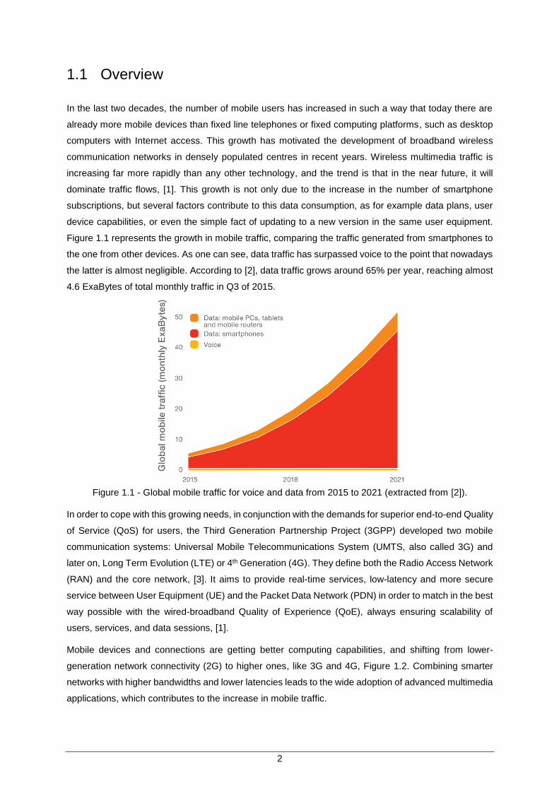
Figure 1.1 represents the growth in mobile traffic, comparing the traffic generated from smartphones to
the one from other devices. As one can see, data traffic has surpassed voice to the point that nowadays
the latter is almost negligible. According to [2], data traffic grows around 65% per year, reaching almost
4.6 ExaBytes of total monthly traffic in Q3 of 2015.
Figure 1.1 - Global mobile traffic for voice and data from 2015 to 2021 (extracted from [2]).
In order to cope with this growing needs, in conjunction with the demands for superior end-to-end Quality
of Service (QoS) for users, the Third Generation Partnership Project (3GPP) developed two mobile
communication systems: Universal Mobile Telecommunications System (UMTS, also called 3G) and
later on, Long Term Evolution (LTE) or 4th Generation (4G). They define both the Radio Access Network
(RAN) and the core network, [3]. It aims to provide real-time services, low-latency and more secure
service between User Equipment (UE) and the Packet Data Network (PDN) in order to match in the best
way possible with the wired-broadband Quality of Experience (QoE), always ensuring scalability of
users, services, and data sessions, [1].
Mobile devices and connections are getting better computing capabilities, and shifting from lower-
generation network connectivity (2G) to higher ones, like 3G and 4G, Figure 1.2. Combining smarter
networks with higher bandwidths and lower latencies leads to the wide adoption of advanced multimedia
applications, which contributes to the increase in mobile traffic.
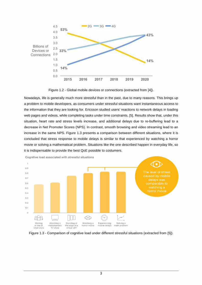
3
Figure 1.2 - Global mobile devices or connections (extracted from [4]).
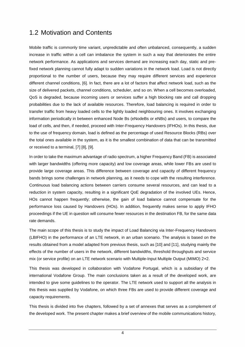
Nowadays, life is generally much more stressful than in the past, due to many reasons. This brings up
a problem to mobile developers, as consumers under stressful situations want instantaneous access to
the information that they are looking for. Ericsson studied users’ reactions to network delays in loading
web pages and videos, while completing tasks under time constraints, [5]. Results show that, under this
situation, heart rate and stress levels increase, and additional delays due to re-buffering lead to a
decrease in Net Promoter Scores (NPS). In contrast, smooth browsing and video streaming lead to an
increase in the same NPS. Figure 1.3 presents a comparison between different situations, where it is
concluded that stress response to mobile delays is similar to that experienced by watching a horror
movie or solving a mathematical problem. Situations like the one described happen in everyday life, so
it is indispensable to provide the best QoE possible to costumers.
Figure 1.3 - Comparison of cognitive load under different stressful situations (extracted from [5]).
4
1.2 Motivation and Contents
Mobile traffic is commonly time variant, unpredictable and often unbalanced, consequently, a sudden
increase in traffic within a cell can imbalance the system in such a way that deteriorates the entire
network performance. As applications and services demand are increasing each day, static and pre-
fixed network planning cannot fully adapt to sudden variations in the network load. Load is not directly
proportional to the number of users, because they may require different services and experience
different channel conditions, [6]. In fact, there are a lot of factors that affect network load, such as the
size of delivered packets, channel conditions, scheduler, and so on. When a cell becomes overloaded,
QoS is degraded, because incoming users or services suffer a high blocking rate and call dropping
probabilities due to the lack of available resources. Therefore, load balancing is required in order to
transfer traffic from heavy loaded cells to the lightly loaded neighbouring ones. It involves exchanging
information periodically in between enhanced Node Bs (eNodeBs or eNBs) and users, to compare the
load of cells, and then, if needed, proceed with Inter-Frequency Handovers (IFHOs). In this thesis, due
to the use of frequency domain, load is defined as the percentage of used Resource Blocks (RBs) over
the total ones available in the system, as it is the smallest combination of data that can be transmitted
or received to a terminal, [7] [8], [9].
In order to take the maximum advantage of radio spectrum, a higher Frequency Band (FB) is associated
with larger bandwidths (offering more capacity) and low coverage areas, while lower FBs are used to
provide large coverage areas. This difference between coverage and capacity of different frequency
bands brings some challenges in network planning, as it needs to cope with the resulting interference.
Continuous load balancing actions between carriers consume several resources, and can lead to a
reduction in system capacity, resulting in a significant QoE degradation of the involved UEs. Hence,
HOs cannot happen frequently; otherwise, the gain of load balance cannot compensate for the
performance loss caused by Handovers (HOs). In addition, frequently makes sense to apply IFHO
proceedings if the UE in question will consume fewer resources in the destination FB, for the same data
rate demands.
The main scope of this thesis is to study the impact of Load Balancing via Inter-Frequency Handovers
(LBIFHO) in the performance of an LTE network, in an urban scenario. The analysis is based on the
results obtained from a model adapted from previous thesis, such as [10] and [11], studying mainly the
effects of the number of users in the network, different bandwidths, threshold throughputs and service
mix (or service profile) on an LTE network scenario with Multiple-Input Multiple Output (MIMO) 2×2.
This thesis was developed in collaboration with Vodafone Portugal, which is a subsidiary of the
international Vodafone Group. The main conclusions taken as a result of the developed work, are
intended to give some guidelines to the operator. The LTE network used to support all the analysis in
this thesis was supplied by Vodafone, on which three FBs are used to provide different coverage and
capacity requirements.
This thesis is divided into five chapters, followed by a set of annexes that serves as a complement of
the developed work. The present chapter makes a brief overview of the mobile communications history,

5
addressing different kind of services demands and in the end, the motivation that leads to the developing
of this thesis.
Chapter 2 presents and introduction to LTE fundamental concepts, covering network architecture, radio
interface, coverage and capacity, services and applications. Particular focus is given to the main issue
under study in this thesis, inter-frequency handovers, and at the end of the chapter, one presents some
of the previously developed works related to load balancing techniques.
A full description of the developed model, as well as the simulator that implements it, are provided in
Chapter 3. The mathematical formulation for further analysis is detailed, with a particular focus on the
antenna gain, as it has an influence on the radius of the sectors, and thus on the coverage area of each
FB. Then, one describes the theoretical models and their implementation in the simulator, wherein each
module is textually detailed. To conclude the chapter, a brief assessment of the model is provided, in
order to ensure the correct functioning of the simulator.
Chapter 4 contains all the analysis of the results extracted from simulations. It begins with a description
of the reference scenario, containing all the parameters used in the simulator, as well as the list of input
and output parameters to be further analysed. Then, the analysis of results follows, addressing the most
relevant information about improvements in the network, essentially related to HOs, capacity and
fairness issues.
Chapter 5 presents the main results, providing the overall conclusions of the obtained results followed
by suggestions for future work. This chapter also summarises the developed work, in order to provide
to the reader a superficial description of the main aspects addressed in this thesis.
At the end, a group of annexes contains additional information within the scope of this thesis. Annex A
provides all the mathematical equations for the calculation of the link budget, between the user and the
BS. Annex B is somehow connected to the previous one, as the path loss is modelled by the COST 231
– Walfisch-Ikegami model. Annex C presents the formulas that relate the received Signal-to-Noise-Ratio
(SNR) with throughput per resource block. Last but not least, Annex D provides the user’s manual to
help in the use of the simulator.

6

7
Chapter 2
Fundamental Concepts and
State of the Art
2 Fundamental Concepts and State of the Art
This chapter provides a brief description on LTE’s fundamental concepts, namely coverage and
capacity, services and applications, inter-frequency handovers, and last but not least, some of the
previous work in the state of the art section.
8
2.1 Network architecture
The implementation of 3GPP Release 8 specifies enhancements to High-Speed Packet Access (HSPA)
access and core networks, as well as the introduction of the Evolved Packet System (EPS), [12]. In
contrast to the previous cellular systems, LTE has been designed only to support packet-switched
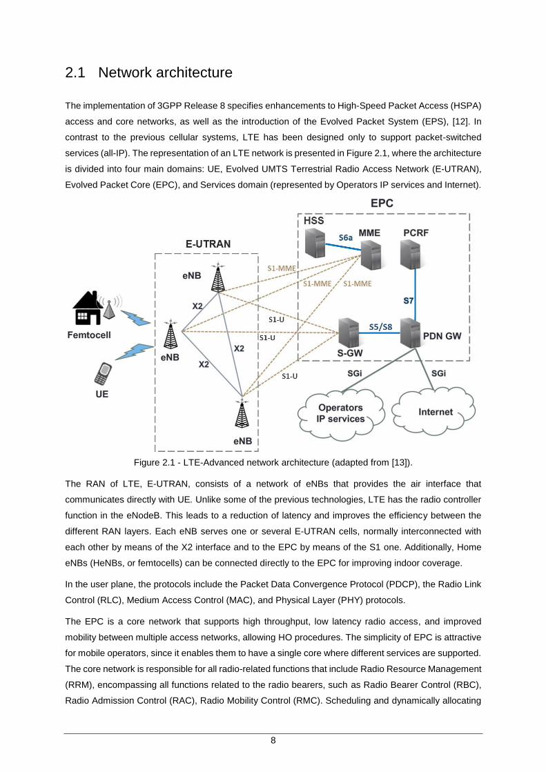
services (all-IP). The representation of an LTE network is presented in Figure 2.1, where the architecture
is divided into four main domains: UE, Evolved UMTS Terrestrial Radio Access Network (E-UTRAN),
Evolved Packet Core (EPC), and Services domain (represented by Operators IP services and Internet).
Figure 2.1 - LTE-Advanced network architecture (adapted from [13]).
The RAN of LTE, E-UTRAN, consists of a network of eNBs that provides the air interface that
communicates directly with UE. Unlike some of the previous technologies, LTE has the radio controller
function in the eNodeB. This leads to a reduction of latency and improves the efficiency between the
different RAN layers. Each eNB serves one or several E-UTRAN cells, normally interconnected with
each other by means of the X2 interface and to the EPC by means of the S1 one. Additionally, Home
eNBs (HeNBs, or femtocells) can be connected directly to the EPC for improving indoor coverage.
In the user plane, the protocols include the Packet Data Convergence Protocol (PDCP), the Radio Link
Control (RLC), Medium Access Control (MAC), and Physical Layer (PHY) protocols.
The EPC is a core network that supports high throughput, low latency radio access, and improved
mobility between multiple access networks, allowing HO procedures. The simplicity of EPC is attractive
for mobile operators, since it enables them to have a single core where different services are supported.
The core network is responsible for all radio-related functions that include Radio Resource Management
(RRM), encompassing all functions related to the radio bearers, such as Radio Bearer Control (RBC),
Radio Admission Control (RAC), Radio Mobility Control (RMC). Scheduling and dynamically allocating
9
radio resources to UE in both up- and downlinks, and always ensuring optimised use of spectrum. The
main logical nodes of EPC are:
S-GW – The Serving Gateway is the terminal node, where all user Internet Protocol (IP) packets
are transferred through, serving as the local mobility anchor for both local inter-eNB handover
and inter-3GPP mobility. It stores the information when the UE is in idle state, and also performs
some administrative functions, such as inter-operator charging (packet routeing and
forwarding). It is connected to the E-UTRAN via S1-U interface.
P-GW – The Packet Data Network Gateway is responsible for IP address assignment for the
UE, as well as filtering user IP packets into different QoS-based bearers, always ensuring a
Guaranteed Bit Rate (GBR), and a flow-based charging according to rules from the PCRF. It
also serves as the mobility anchor for interworking with non-3GPP access networks.
PCRF – The Policy Control and Charging Rules Function is responsible for policy control
decision-making, as well as for controlling the charging functionalities in the P-GW. This was a
major change from previous networks, where service control was realised primarily through UE
authentication by the network. The PCRF provides the QoS authorisation according to the users’
subscription profile.
MME - Mobility Management Entity is the control node that processes the signalling between
the UE and the CN, and it is in charge of managing security functions (authentication,
authorisation for both signalling and user data), handling idle state mobility, roaming, and
handovers. MME also selects the S-GW and P-GW nodes and is connected to the eNB through
S1-MME interface.
HSS – The Home Subscriber Server that stores user subscription information, determining the
identity and privileges of a user and tracking activities via Authorisation, Authentication and
Accounting (AAA) server, and enforcing charging and QoS policies through PCRF. In addition,
the HSS holds dynamic information, such as the identity of the MME to which the user is
currently attached or registered, [1], [3], [14], [15], [16].
2.2 Radio interface
Usually, mobile radio channels tend to be dispersive and time-variant, so in order to achieve the best
system performance for wireless communications, it is crucial to choose an appropriate modulation and
multiple access technique. There are two multiple access techniques applied in LTE: Orthogonal
Frequency-Division Multiple Access (OFDMA) in the Downlink (DL) and Single-Carrier Frequency-
Division Multiple Access (SC-FDMA) for Uplink (UL), [17]. A multicarrier scheme is a technique that
subdivides the used channel bandwidth into a number of parallel sub-channels, [18].
Orthogonal Frequency-Division Multiplexing (OFDM) offers robustness against multipath transmission,
and this can be achieved by the split of the data stream into a high number of narrowband orthogonal
subcarriers spaced by 15 kHz. By the addition of a guard interval, the Cycle Prefix (CP), this multicarrier
10
scheme is resilient against Inter-Symbol Interference (ISI) or Inter-Carrier Interference (ICI). These
degradations are avoided as long as the CP is longer than the maximum excess delay of the channel.
Since these subcarriers are mutually orthogonal, overlapping between them is allowed, leading to a
highly spectral efficient system. Still, OFDM also presents some drawbacks, as sensitivity to Doppler
shift and inefficient power consumption due to high Peak-Average-Ratio (PAR), [19], [17], [20].
SC-FDMA basically has the same benefits of OFDMA in terms of multipath resistance and frequency
allocation flexibility, but with the advantage that is more power efficient than OFDMA, saving battery for
the UE. This property makes SC-FDMA attractive for UL, [21]. Last but not least, since this scheme uses
orthogonal transmission, intra-cell interference, where UEs interfere with each other, is minimised
compared to other 3GPP systems.
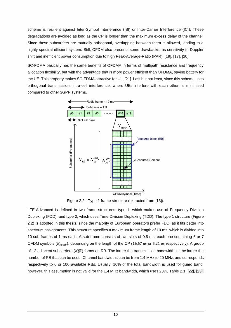
Figure 2.2 - Type 1 frame structure (extracted from [13]).
LTE-Advanced is defined in two frame structures: type 1, which makes use of Frequency Division
Duplexing (FDD), and type 2, which uses Time Division Duplexing (TDD). The type 1 structure (Figure
2.2) is adopted in this thesis, since the majority of European operators prefer FDD, as it fits better into
spectrum assignments. This structure specifies a maximum frame length of 10 ms, which is divided into
10 sub-frames of 1 ms each. A sub-frame consists of two slots of 0.5 ms, each one containing 6 or 7
OFDM symbols (𝑁𝑠𝑦𝑚𝑏), depending on the length of the CP (16.67 𝜇𝑠 or 5.21 𝜇𝑠 respectively). A group
of 12 adjacent subcarriers (𝑁𝑆𝐶𝑅𝐵) forms an RB. The larger the transmission bandwidth is, the larger the
number of RB that can be used. Channel bandwidths can be from 1.4 MHz to 20 MHz, and corresponds
respectively to 6 or 100 available RBs. Usually, 10% of the total bandwidth is used for guard band;
however, this assumption is not valid for the 1.4 MHz bandwidth, which uses 23%, Table 2.1, [22], [23].
11
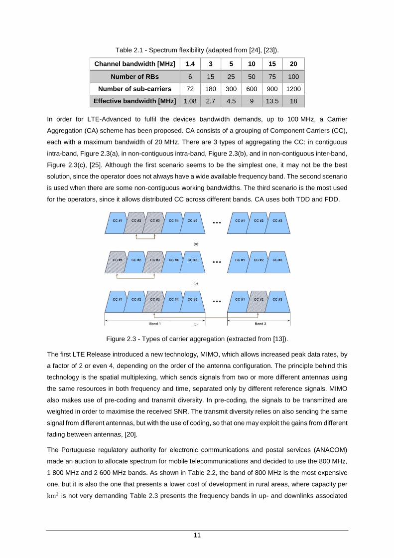
Table 2.1 - Spectrum flexibility (adapted from [24], [23]).
Channel bandwidth [MHz] 1.4 3 5 10 15 20
Number of RBs 6 15 25 50 75 100
Number of sub-carriers 72 180 300 600 900 1200
Effective bandwidth [MHz] 1.08 2.7 4.5 9 13.5 18
In order for LTE-Advanced to fulfil the devices bandwidth demands, up to 100 MHz, a Carrier
Aggregation (CA) scheme has been proposed. CA consists of a grouping of Component Carriers (CC),
each with a maximum bandwidth of 20 MHz. There are 3 types of aggregating the CC: in contiguous
intra-band, Figure 2.3(a), in non-contiguous intra-band, Figure 2.3(b), and in non-contiguous inter-band,
Figure 2.3(c), [25]. Although the first scenario seems to be the simplest one, it may not be the best
solution, since the operator does not always have a wide available frequency band. The second scenario
is used when there are some non-contiguous working bandwidths. The third scenario is the most used
for the operators, since it allows distributed CC across different bands. CA uses both TDD and FDD.
Figure 2.3 - Types of carrier aggregation (extracted from [13]).
The first LTE Release introduced a new technology, MIMO, which allows increased peak data rates, by
a factor of 2 or even 4, depending on the order of the antenna configuration. The principle behind this
technology is the spatial multiplexing, which sends signals from two or more different antennas using
the same resources in both frequency and time, separated only by different reference signals. MIMO
also makes use of pre-coding and transmit diversity. In pre-coding, the signals to be transmitted are
weighted in order to maximise the received SNR. The transmit diversity relies on also sending the same
signal from different antennas, but with the use of coding, so that one may exploit the gains from different
fading between antennas, [20].
The Portuguese regulatory authority for electronic communications and postal services (ANACOM)
made an auction to allocate spectrum for mobile telecommunications and decided to use the 800 MHz,
1 800 MHz and 2 600 MHz bands. As shown in Table 2.2, the band of 800 MHz is the most expensive
one, but it is also the one that presents a lower cost of development in rural areas, where capacity per
km2 is not very demanding Table 2.3 presents the frequency bands in up- and downlinks associated
12
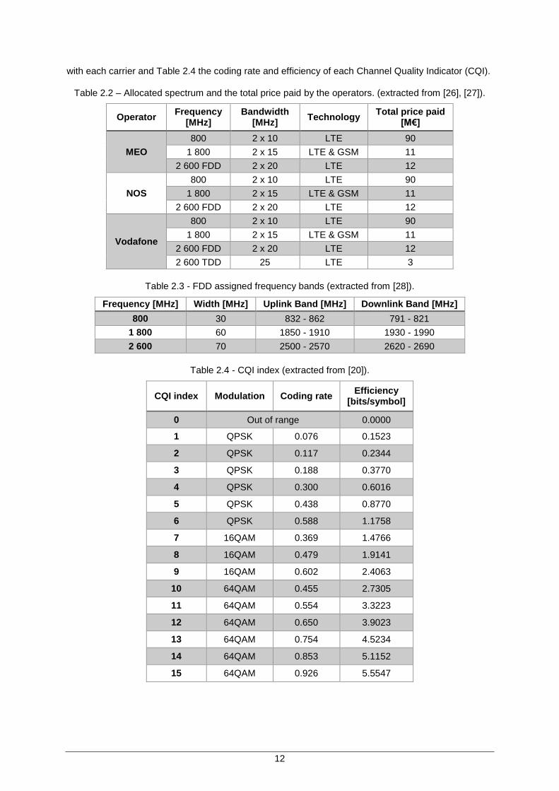
with each carrier and Table 2.4 the coding rate and efficiency of each Channel Quality Indicator (CQI).
Table 2.2 – Allocated spectrum and the total price paid by the operators. (extracted from [26], [27]).
Operator Frequency
[MHz] Bandwidth
[MHz] Technology
Total price paid [M€]
MEO
800 2 x 10 LTE 90
1 800 2 x 15 LTE & GSM 11
2 600 FDD 2 x 20 LTE 12
NOS
800 2 x 10 LTE 90
1 800 2 x 15 LTE & GSM 11
2 600 FDD 2 x 20 LTE 12
Vodafone
800 2 x 10 LTE 90
1 800 2 x 15 LTE & GSM 11
2 600 FDD 2 x 20 LTE 12
2 600 TDD 25 LTE 3
Table 2.3 - FDD assigned frequency bands (extracted from [28]).
Frequency [MHz] Width [MHz] Uplink Band [MHz] Downlink Band [MHz]
800 30 832 - 862 791 - 821
1 800 60 1850 - 1910 1930 - 1990
2 600 70 2500 - 2570 2620 - 2690
Table 2.4 - CQI index (extracted from [20]).
CQI index Modulation Coding rate Efficiency
[bits/symbol]
0 Out of range 0.0000
1 QPSK 0.076 0.1523
2 QPSK 0.117 0.2344
3 QPSK 0.188 0.3770
4 QPSK 0.300 0.6016
5 QPSK 0.438 0.8770
6 QPSK 0.588 1.1758
7 16QAM 0.369 1.4766
8 16QAM 0.479 1.9141
9 16QAM 0.602 2.4063
10 64QAM 0.455 2.7305
11 64QAM 0.554 3.3223
12 64QAM 0.650 3.9023
13 64QAM 0.754 4.5234
14 64QAM 0.853 5.1152
15 64QAM 0.926 5.5547
13
2.3 Coverage and capacity
With the growth in wireless traffic, in order to serve a zone like a mall or an office, a small-size low-
power Base Station (BS) can be introduced within the serving eNB, which is referred to as
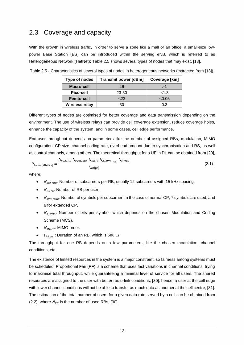
Heterogeneous Network (HetNet); Table 2.5 shows several types of nodes that may exist, [13].
Table 2.5 - Characteristics of several types of nodes in heterogeneous networks (extracted from [13]).
Type of nodes Transmit power [dBm] Coverage [km]
Macro-cell 46 >1
Pico-cell 23-30 <1.3
Femto-cell <23 <0.05
Wireless relay 30 0.3
Different types of nodes are optimised for better coverage and data transmission depending on the
environment. The use of wireless relays can provide cell coverage extension, reduce coverage holes,
enhance the capacity of the system, and in some cases, cell edge performance.
End-user throughput depends on parameters like the number of assigned RBs, modulation, MIMO
configuration, CP size, channel coding rate, overhead amount due to synchronisation and RS, as well
as control channels, among others. The theoretical throughput for a UE in DL can be obtained from [29],
𝑅𝑏,𝑡𝑒𝑜 [Mbit s⁄ ] =𝑁𝑠𝑢𝑏/𝑅𝐵 𝑁𝑠𝑦𝑚/𝑠𝑢𝑏 𝑁𝑅𝐵/𝑢 𝑁𝑏/𝑠𝑦𝑚[bit]
𝑁𝑀𝐼𝑀𝑂
𝑡𝑅𝐵[μs] (2.1)
where:
𝑁𝑠𝑢𝑏/𝑅𝐵: Number of subcarriers per RB, usually 12 subcarriers with 15 kHz spacing.
𝑁𝑅𝐵/𝑢: Number of RB per user.
𝑁𝑠𝑦𝑚/𝑠𝑢𝑏: Number of symbols per subcarrier. In the case of normal CP, 7 symbols are used, and
6 for extended CP.
𝑁𝑏/𝑠𝑦𝑚: Number of bits per symbol, which depends on the chosen Modulation and Coding
Scheme (MCS).
𝑁𝑀𝐼𝑀𝑂: MIMO order.
𝑡𝑅𝐵[μs]: Duration of an RB, which is 500 μs.
The throughput for one RB depends on a few parameters, like the chosen modulation, channel
conditions, etc.
The existence of limited resources in the system is a major constraint, so fairness among systems must
be scheduled. Proportional Fair (PF) is a scheme that uses fast variations in channel conditions, trying
to maximise total throughput, while guaranteeing a minimal level of service for all users. The shared
resources are assigned to the user with better radio-link conditions, [30], hence, a user at the cell edge
with lower channel conditions will not be able to transfer as much data as another at the cell centre, [31].
The estimation of the total number of users for a given data rate served by a cell can be obtained from
(2.2), where 𝑁𝑅𝐵 is the number of used RBs, [30].
14
𝑁𝑢 =𝑁𝑠𝑢𝑏/𝑅𝐵 𝑁𝑠𝑦𝑚/𝑠𝑢𝑏 𝑁𝑅𝐵 𝑁𝑏/𝑠𝑦𝑚[bit]
𝑁𝑀𝐼𝑀𝑂
𝑅𝑏 [Mbps] 𝑡𝑅𝐵[μs] (2.2)
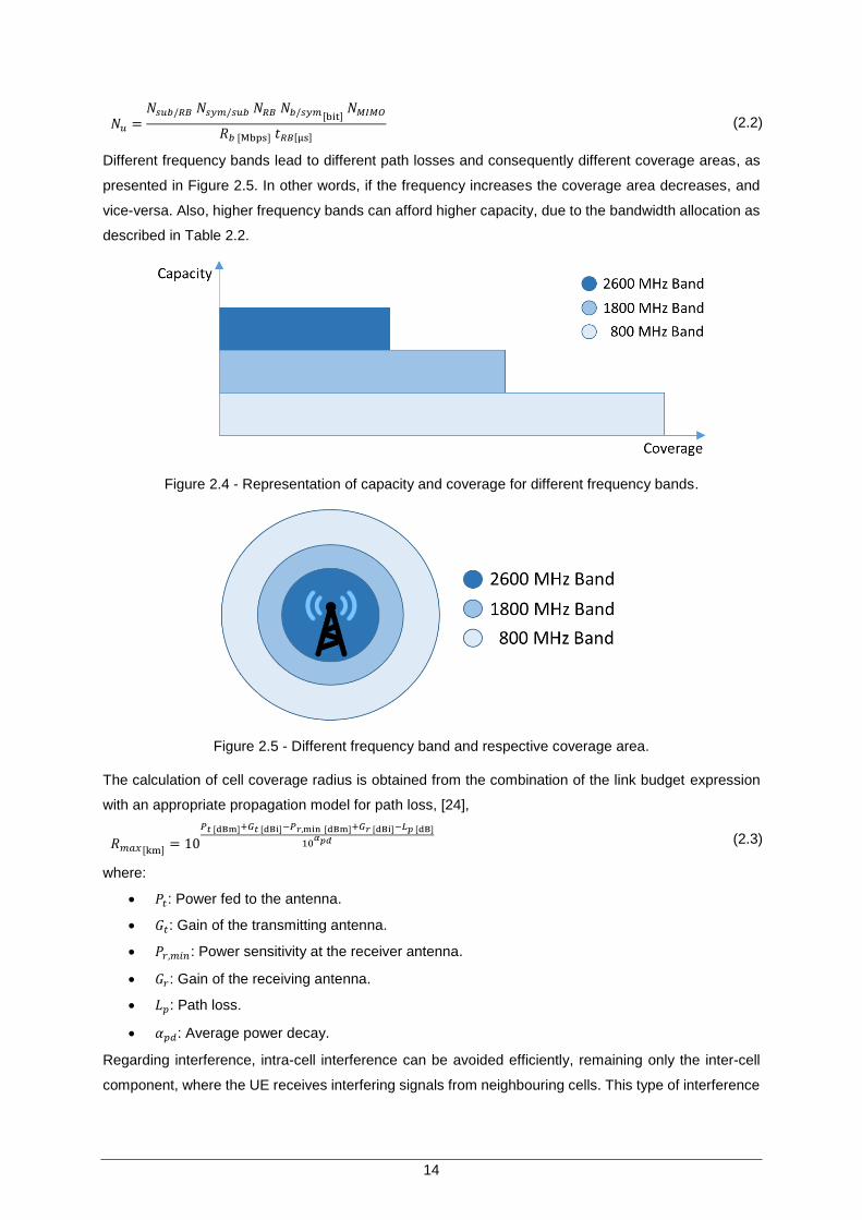
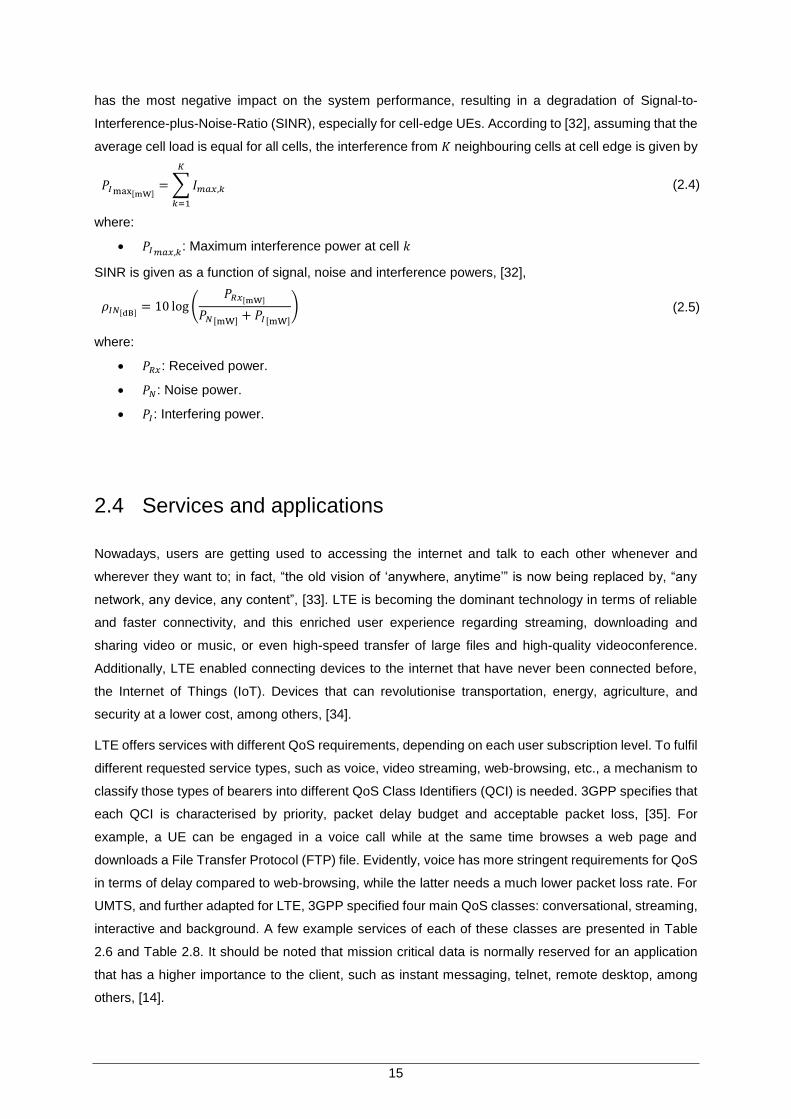
Different frequency bands lead to different path losses and consequently different coverage areas, as
presented in Figure 2.5. In other words, if the frequency increases the coverage area decreases, and
vice-versa. Also, higher frequency bands can afford higher capacity, due to the bandwidth allocation as
described in Table 2.2.
Figure 2.4 - Representation of capacity and coverage for different frequency bands.
Figure 2.5 - Different frequency band and respective coverage area.
The calculation of cell coverage radius is obtained from the combination of the link budget expression
with an appropriate propagation model for path loss, [24],
𝑅𝑚𝑎𝑥[km] = 10
𝑃𝑡 [dBm]+𝐺𝑡 [dBi]−𝑃𝑟,min [dBm]+𝐺𝑟 [dBi]−𝐿𝑝 [dB]
10𝛼𝑝𝑑 (2.3)
where:
𝑃𝑡: Power fed to the antenna.
𝐺𝑡: Gain of the transmitting antenna.
𝑃𝑟,𝑚𝑖𝑛: Power sensitivity at the receiver antenna.
𝐺𝑟: Gain of the receiving antenna.
𝐿𝑝: Path loss.
𝛼𝑝𝑑: Average power decay.
Regarding interference, intra-cell interference can be avoided efficiently, remaining only the inter-cell
component, where the UE receives interfering signals from neighbouring cells. This type of interference
15
has the most negative impact on the system performance, resulting in a degradation of Signal-to-
Interference-plus-Noise-Ratio (SINR), especially for cell-edge UEs. According to [32], assuming that the
average cell load is equal for all cells, the interference from 𝐾 neighbouring cells at cell edge is given by
𝑃𝐼max[mW]= ∑ 𝐼𝑚𝑎𝑥,𝑘
𝐾
𝑘=1
(2.4)
where:
𝑃𝐼𝑚𝑎𝑥,𝑘: Maximum interference power at cell 𝑘
SINR is given as a function of signal, noise and interference powers, [32],
𝜌𝐼𝑁[dB]= 10 log (
𝑃𝑅𝑥[mW]
𝑃𝑁[mW] + 𝑃𝐼[mW]
) (2.5)
where:
𝑃𝑅𝑥: Received power.
𝑃𝑁: Noise power.
𝑃𝐼: Interfering power.
2.4 Services and applications
Nowadays, users are getting used to accessing the internet and talk to each other whenever and
wherever they want to; in fact, “the old vision of ‘anywhere, anytime’” is now being replaced by, “any
network, any device, any content”, [33]. LTE is becoming the dominant technology in terms of reliable
and faster connectivity, and this enriched user experience regarding streaming, downloading and
sharing video or music, or even high-speed transfer of large files and high-quality videoconference.
Additionally, LTE enabled connecting devices to the internet that have never been connected before,
the Internet of Things (IoT). Devices that can revolutionise transportation, energy, agriculture, and
security at a lower cost, among others, [34].
LTE offers services with different QoS requirements, depending on each user subscription level. To fulfil
different requested service types, such as voice, video streaming, web-browsing, etc., a mechanism to
classify those types of bearers into different QoS Class Identifiers (QCI) is needed. 3GPP specifies that
each QCI is characterised by priority, packet delay budget and acceptable packet loss, [35]. For
example, a UE can be engaged in a voice call while at the same time browses a web page and
downloads a File Transfer Protocol (FTP) file. Evidently, voice has more stringent requirements for QoS
in terms of delay compared to web-browsing, while the latter needs a much lower packet loss rate. For
UMTS, and further adapted for LTE, 3GPP specified four main QoS classes: conversational, streaming,
interactive and background. A few example services of each of these classes are presented in Table
2.6 and Table 2.8. It should be noted that mission critical data is normally reserved for an application
that has a higher importance to the client, such as instant messaging, telnet, remote desktop, among
others, [14].
16
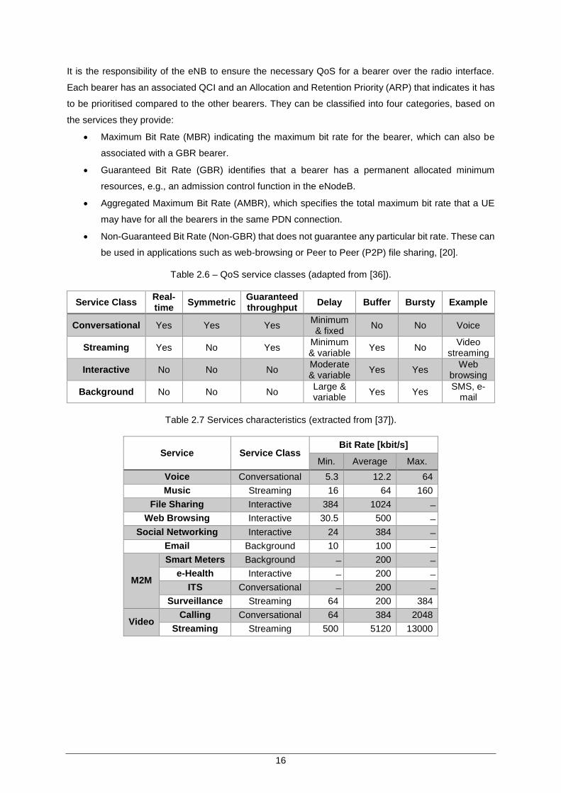
It is the responsibility of the eNB to ensure the necessary QoS for a bearer over the radio interface.
Each bearer has an associated QCI and an Allocation and Retention Priority (ARP) that indicates it has
to be prioritised compared to the other bearers. They can be classified into four categories, based on
the services they provide:
Maximum Bit Rate (MBR) indicating the maximum bit rate for the bearer, which can also be
associated with a GBR bearer.
Guaranteed Bit Rate (GBR) identifies that a bearer has a permanent allocated minimum
resources, e.g., an admission control function in the eNodeB.
Aggregated Maximum Bit Rate (AMBR), which specifies the total maximum bit rate that a UE
may have for all the bearers in the same PDN connection.
Non-Guaranteed Bit Rate (Non-GBR) that does not guarantee any particular bit rate. These can
be used in applications such as web-browsing or Peer to Peer (P2P) file sharing, [20].
Table 2.6 – QoS service classes (adapted from [36]).
Service Class Real-time
Symmetric Guaranteed throughput
Delay Buffer Bursty Example
Conversational Yes Yes Yes Minimum & fixed
No No Voice
Streaming Yes No Yes Minimum & variable
Yes No Video
streaming
Interactive No No No Moderate & variable
Yes Yes Web
browsing
Background No No No Large & variable
Yes Yes SMS, e-
Table 2.7 Services characteristics (extracted from [37]).
Service Service Class Bit Rate [kbit/s]
Min. Average Max.
Voice Conversational 5.3 12.2 64
Music Streaming 16 64 160
File Sharing Interactive 384 1024 ̶
Web Browsing Interactive 30.5 500 ̶
Social Networking Interactive 24 384 ̶
Email Background 10 100 ̶
M2M
Smart Meters Background ̶ 200 ̶
e-Health Interactive ̶ 200 ̶
ITS Conversational ̶ 200 ̶
Surveillance Streaming 64 200 384
Video Calling Conversational 64 384 2048
Streaming Streaming 500 5120 13000
17
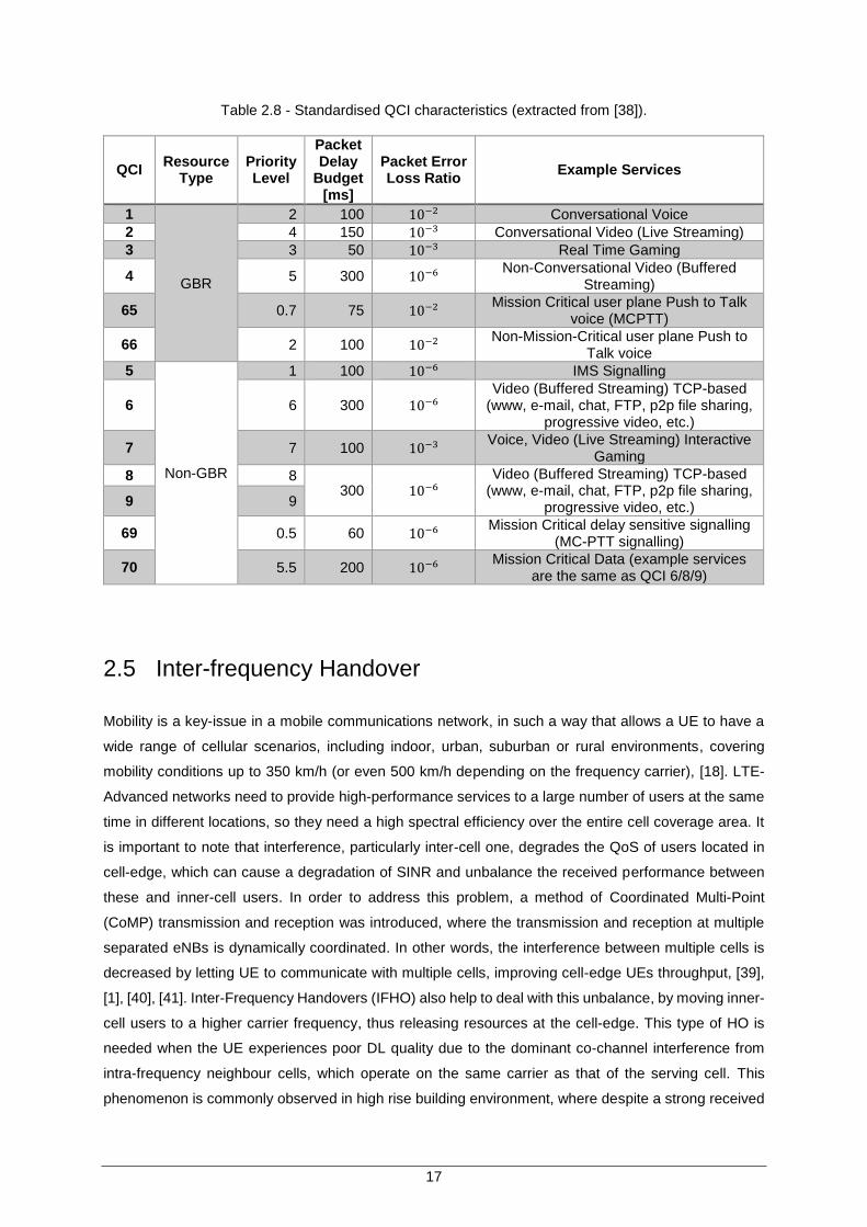
Table 2.8 - Standardised QCI characteristics (extracted from [38]).
QCI Resource
Type Priority Level
Packet Delay
Budget [ms]
Packet Error Loss Ratio
Example Services
1
GBR
2 100 10−2 Conversational Voice
2 4 150 10−3 Conversational Video (Live Streaming)
3 3 50 10−3 Real Time Gaming
4 5 300 10−6 Non-Conversational Video (Buffered
Streaming)
65 0.7 75 10−2 Mission Critical user plane Push to Talk
voice (MCPTT)
66 2 100 10−2 Non-Mission-Critical user plane Push to
Talk voice
5
Non-GBR
1 100 10−6 IMS Signalling
6 6 300 10−6 Video (Buffered Streaming) TCP-based
(www, e-mail, chat, FTP, p2p file sharing, progressive video, etc.)
7 7 100 10−3 Voice, Video (Live Streaming) Interactive
Gaming
8 8 300 10−6
Video (Buffered Streaming) TCP-based (www, e-mail, chat, FTP, p2p file sharing,
progressive video, etc.) 9 9
69 0.5 60 10−6 Mission Critical delay sensitive signalling
(MC-PTT signalling)
70 5.5 200 10−6 Mission Critical Data (example services
are the same as QCI 6/8/9)
2.5 Inter-frequency Handover
Mobility is a key-issue in a mobile communications network, in such a way that allows a UE to have a
wide range of cellular scenarios, including indoor, urban, suburban or rural environments, covering
mobility conditions up to 350 km/h (or even 500 km/h depending on the frequency carrier), [18]. LTE-
Advanced networks need to provide high-performance services to a large number of users at the same
time in different locations, so they need a high spectral efficiency over the entire cell coverage area. It
is important to note that interference, particularly inter-cell one, degrades the QoS of users located in
cell-edge, which can cause a degradation of SINR and unbalance the received performance between
these and inner-cell users. In order to address this problem, a method of Coordinated Multi-Point
(CoMP) transmission and reception was introduced, where the transmission and reception at multiple
separated eNBs is dynamically coordinated. In other words, the interference between multiple cells is
decreased by letting UE to communicate with multiple cells, improving cell-edge UEs throughput, [39],
[1], [40], [41]. Inter-Frequency Handovers (IFHO) also help to deal with this unbalance, by moving inner-
cell users to a higher carrier frequency, thus releasing resources at the cell-edge. This type of HO is
needed when the UE experiences poor DL quality due to the dominant co-channel interference from
intra-frequency neighbour cells, which operate on the same carrier as that of the serving cell. This
phenomenon is commonly observed in high rise building environment, where despite a strong received
18
signal strength, the received signal quality can be poor due to the strong inter-cell interference
originating from neighbour cells. In such scenario, an intra-frequency handover is less likely to improve
the received quality signal, since in other intra-frequency neighbour cells the UE is expected to
experience a similar level of interference, [42].
As mentioned above, HOs are the main key regarding load balancing in LTE. There are essentially two
main types:
Intra-frequency handover, as it is name suggests, is a HO in which the UE remains in the same
channel and frequency, and merely moves to another cell on the same network. Typically, it is
performed by eNBs, by means of the X2 interface, but it may require a change to the MME
and/or S-GW if the UE moves to another cell.
Inter-frequency handover, which means that the UE moves to a different carrier, being usually
associated with intra-eNB or intra-cell handover, where the UE remains in the same cell.
The most common scenario for use of IFHO is when the UE reaches the coverage edge of the current
serving frequency layer and thereby needs to make a coverage based inter-frequency handover. An
IFHO allows an operator to retain service quality, load balancing, retaining cell coverage etc. depending
on the needs. The focus of this thesis is to evaluate the second objective, which is balancing users via
IFHO, [42], [43].
Load balancing techniques specify two states for the UE: active or idle mode. In the active load balancing
mode or Radio Resource Control connected state (RCC_CONNECTED), HOs are network controlled,
based on UE measurements, when it sends or receives data. The E-UTRAN decides when to make the
HO and which is the target cell, depending on UE traffic requirements and radio conditions. In idle mode
(RCC_IDLE), the load balancing is more difficult to achieve, because eNBs can only detect a user when
it becomes active or when it changes the tracking area. In this mode, the UE is responsible for choosing
and then registering in the most suitable cell, based on measurements of received broadcast channels
of the Public Land Mobile Network (PLMN), a process known as cell selection. This selection requires
that the cell is not overloaded and that the quality of the channel is good enough. Inter-frequency load
balancing is controlled by the cell reselection procedure; if the UE finds a cell outside its tracking area,
a location registration needs to be performed. On the other hand, if the UE cannot find a suitable for
camping or if the location registration fails, it enters in a “limited service” state and only emergency calls
can be made. Since system parameters and radio resource preferences are transmitted to the UE by
means of System Information Blocks (SIBs), it is possible for an eNB to force a user in a cell edge to
select the one with the highest transmitted power, or force a HO to a different carrier with more available
resources, [8], [20].
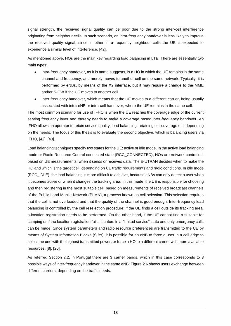
As referred Section 2.2, in Portugal there are 3 carrier bands, which in this case corresponds to 3
possible ways of inter-frequency handover in the same eNB; Figure 2.6 shows users exchange between
different carriers, depending on the traffic needs.
19
Figure 2.6 - Different scenarios for IFHO.
In order to guarantee an efficient use of multiple carrier frequencies deployed in the same coverage
area, 3GPP E-UTRAN standards define radio resource management requirements, procedures and
mechanisms related to IFHO, [44]. To support inter-frequency and intra-RAT mobility in E-UTRAN, the
HO decision is taken by the serving cell and relies on one or more DL measurements reported by the
UE to identify inter-frequency cells, [45], [46]: Reference Symbol Received Power (RSRP) and
Reference Symbol Received Quality (RSRQ). Based on these measurements, the serving cell decides
whether to perform HO or nor, by sending or not the HO command.
RSRP corresponds to the measured signal strength, being defined by the average of the received power
of the resource elements within the considered measurement frequency bandwidth. RSRQ represents
the cell quality, being defined as the ratio between RSRP and E-UTRA carrier Received Signal Strength
Indicator (RSSI), and depends on the number of RBs over the measurement bandwidth. The RSSI is
the linear average of the total received power in OFDM symbols containing the reference symbols, [22].
According to [47] and [48], RSRP and RSRQ is given by (2.6) and (2.7), respectively.
𝑃𝑅𝑆𝑅𝑃[dBm]= 10 log10 (
∑ 𝑃𝑟,𝑅𝐸,𝑘 [mW]𝑁𝑅𝐸𝑘=1
𝑁𝑅𝐸
) (2.6)
where:
𝑁𝑅𝐸: Number of resource elements (REs).
𝑃𝑟,𝑅𝐸,𝑘 [mW]: Estimated received power of the 𝑘𝑡ℎ RE.
𝑃𝑅𝑆𝑅𝑄[dB]= 𝑁𝑅𝐵/𝑢 (𝑃𝑅𝑆𝑅𝑃[dBm]
− 𝑃𝑅𝑆𝑆𝐼[dBm]) (2.7)
2.6 State of the art
There were several proposals to solve load balancing problems by using an HO scheme. According to
[49], the most popular one is “adaptive cell sizing”, which uses the tuning pilot power of the BSs in order
to force UEs from cell edge to HO to the neighbouring cell with the strongest RSRP. However, this
scheme brings some disadvantages, e.g., some UEs may be not covered by any BSs, [6]. Another much
used HO algorithm makes decisions based on the SINR, but this also has some drawbacks; it does not
take UEs’ QoS requirements and the load of the other cells/sectors into account, [50].
As referred before, an HO scheme only based on RSRP is not always the best solution. The authors in
[51] propose an evaluation of five methods of inter-frequency quality handover for voice traffic, since it
is the one with more restrict requirements. It compares system performance using RSRP, RSRQ and a
20
combination of both in synchronous and asynchronous setups, for low and high network load scenario.
In the synchronous network setup, the frame timings of all simulated cells are assumed to be perfectly
aligned; in an asynchronous network, the frame timing of each cell is set independently. To evaluate the
performance of the different IFHO methods, it was assumed that the voice user is not dropped due to
the bad link quality, instead a voice packet being discarded if not delivered within 80 ms, 1% is the
maximum packet loss rate and the most suitable HO criterion should correspond to the lower number
of handovers. Results show that the variations in RSRP, in contrast to RSRQ, do not depend on the
network load, since it only measures the power of the reference signal. Also, an IFHO based only on
RSRP significantly increases the number of handovers, while one based only on RSRQ reduces it, but
slightly increases the packet loss rate. The authors in [43] also confirm that the observed number of
HOs is very high, even with the widest measurement bandwidths and using PF scheduler, if no filtering
over consecutive measurements gap is considered. It is verified that fast variations in RSRQ are avoided
by the use of Round-Robin (RR) scheduling, and a higher layer time domain filter. The overall best
performance is achieved when the HO criterion uses both RSRP and RSRQ, and thus guarantees the
desired received pilot strength, voice packet loss rate remains below the 1% target level, as well as
ensuring that the signal quality stays within the limits after handover.
In more challenging DL limited scenarios, which are often encountered in a street between tall buildings,
RSRQ based HO schemes are likely to provide even more gain in terms of reduced number of IFHOs.
Furthermore, in a scenario based only on RSRP would cause even a higher packet loss rate, since
worse DL quality is likely to be experienced due to the delay in the HO process.
In [6], a cell is considered overloaded when the packet drop rate is over 20%. It also defines some
performance criteria for voice over IP (VoIP) users; the maximum call delay is 60 ms, and the call will
drop if the packet drop rate is over 40%. When a cell is full, some packets may fail to be allocated, and
in this case, they are stored in a queue to be later delivered. QoS is defined as the combination of HO
users packet drop rate and HO packet drop rate. A measurement is performed to compare the
performance between the proposed inter-frequency handover algorithm and the tuning pilot power
algorithm by means of packet drop rate, QoS failure user rate, number of HO users and HO latency.
Using the proposed algorithm, it is concluded that the packet drop ratio is reduced to less than 40%, the
call drop ratio to 30%, and the HO latency to the limit of 50 ms, fulfilling the requirements of Table 2.8.
The aim of [7] is to balance traffic load, improving system performance and minimising the number of
HOs by means of a proposed Mobility Load Balancing (MLB) algorithm. The goal of this algorithm is to
minimise the average system delay and the average number of HOs in order not to overload the system
with signalling and control. The procedure stabilises the system and makes a trade-off between the
average queue backlog and the number of HOs. Considering these two motivations, a penalty factor
([0, 1]) is proposed for incoming HO requests. In the case of a larger penalty factor, the algorithm
chooses to reduce the number of HOs, at the cost of the larger average queue backlog, resulting in a
larger average system delay. On the other hand, with the smaller penalty factor, it prefers to have the
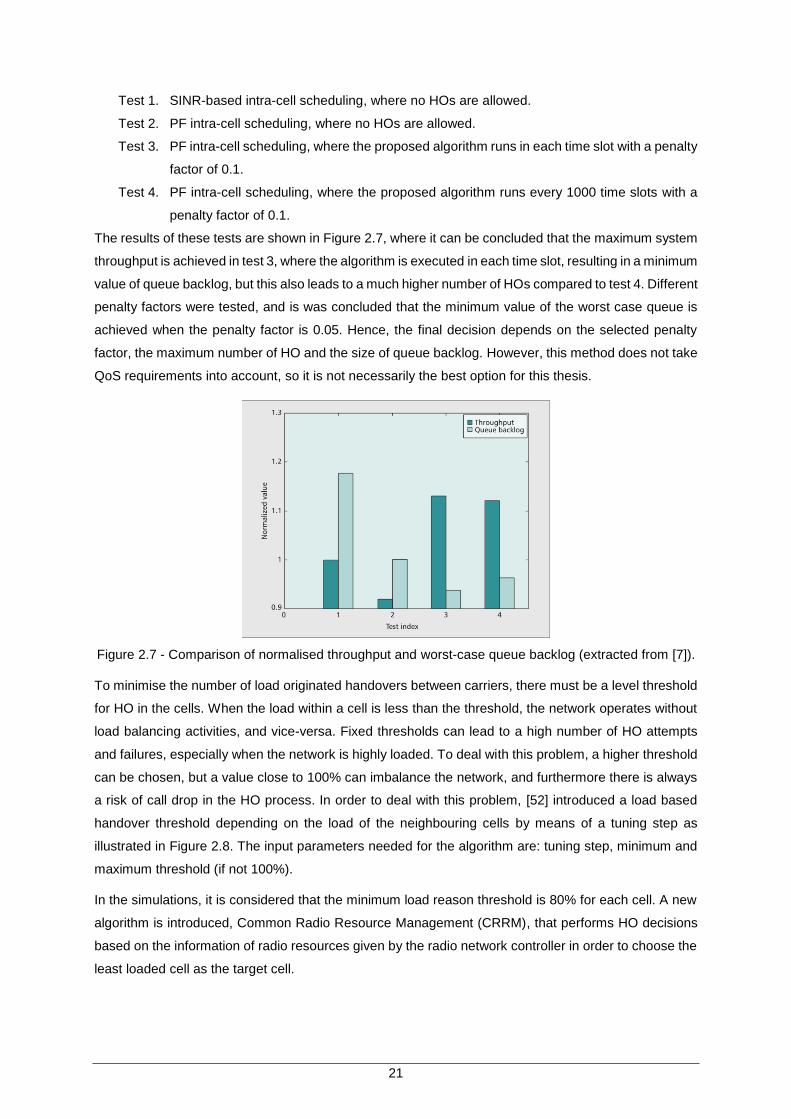
shorter system delay with an increased number of HOs. Four tests are performed in order to analyse
the throughput and the queue backlog:
21
Test 1. SINR-based intra-cell scheduling, where no HOs are allowed.
Test 2. PF intra-cell scheduling, where no HOs are allowed.
Test 3. PF intra-cell scheduling, where the proposed algorithm runs in each time slot with a penalty
factor of 0.1.
Test 4. PF intra-cell scheduling, where the proposed algorithm runs every 1000 time slots with a
penalty factor of 0.1.
The results of these tests are shown in Figure 2.7, where it can be concluded that the maximum system
throughput is achieved in test 3, where the algorithm is executed in each time slot, resulting in a minimum
value of queue backlog, but this also leads to a much higher number of HOs compared to test 4. Different
penalty factors were tested, and is was concluded that the minimum value of the worst case queue is
achieved when the penalty factor is 0.05. Hence, the final decision depends on the selected penalty
factor, the maximum number of HO and the size of queue backlog. However, this method does not take
QoS requirements into account, so it is not necessarily the best option for this thesis.
Figure 2.7 - Comparison of normalised throughput and worst-case queue backlog (extracted from [7]).
To minimise the number of load originated handovers between carriers, there must be a level threshold
for HO in the cells. When the load within a cell is less than the threshold, the network operates without
load balancing activities, and vice-versa. Fixed thresholds can lead to a high number of HO attempts
and failures, especially when the network is highly loaded. To deal with this problem, a higher threshold
can be chosen, but a value close to 100% can imbalance the network, and furthermore there is always
a risk of call drop in the HO process. In order to deal with this problem, [52] introduced a load based
handover threshold depending on the load of the neighbouring cells by means of a tuning step as
illustrated in Figure 2.8. The input parameters needed for the algorithm are: tuning step, minimum and
maximum threshold (if not 100%).
In the simulations, it is considered that the minimum load reason threshold is 80% for each cell. A new
algorithm is introduced, Common Radio Resource Management (CRRM), that performs HO decisions
based on the information of radio resources given by the radio network controller in order to choose the
least loaded cell as the target cell.
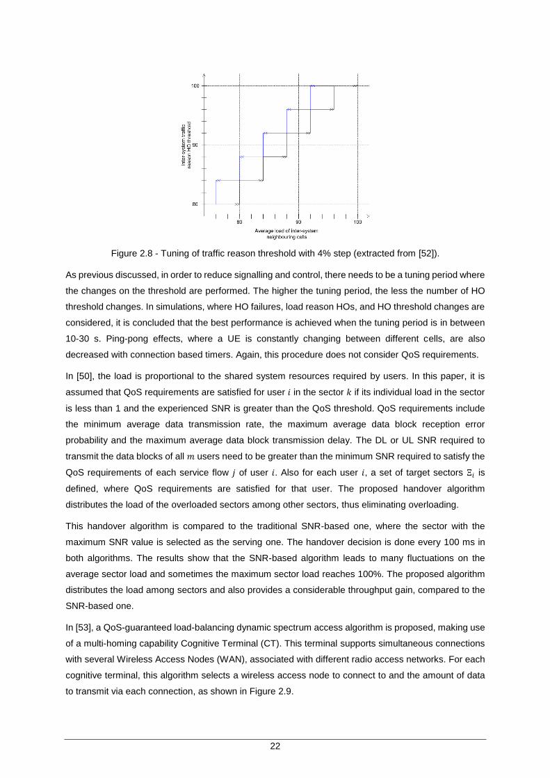
22
Figure 2.8 - Tuning of traffic reason threshold with 4% step (extracted from [52]).
As previous discussed, in order to reduce signalling and control, there needs to be a tuning period where
the changes on the threshold are performed. The higher the tuning period, the less the number of HO
threshold changes. In simulations, where HO failures, load reason HOs, and HO threshold changes are
considered, it is concluded that the best performance is achieved when the tuning period is in between
10-30 s. Ping-pong effects, where a UE is constantly changing between different cells, are also
decreased with connection based timers. Again, this procedure does not consider QoS requirements.
In [50], the load is proportional to the shared system resources required by users. In this paper, it is
assumed that QoS requirements are satisfied for user 𝑖 in the sector 𝑘 if its individual load in the sector
is less than 1 and the experienced SNR is greater than the QoS threshold. QoS requirements include
the minimum average data transmission rate, the maximum average data block reception error
probability and the maximum average data block transmission delay. The DL or UL SNR required to
transmit the data blocks of all 𝑚 users need to be greater than the minimum SNR required to satisfy the
QoS requirements of each service flow 𝑗 of user 𝑖. Also for each user 𝑖, a set of target sectors Ξ𝑖 is
defined, where QoS requirements are satisfied for that user. The proposed handover algorithm
distributes the load of the overloaded sectors among other sectors, thus eliminating overloading.
This handover algorithm is compared to the traditional SNR-based one, where the sector with the
maximum SNR value is selected as the serving one. The handover decision is done every 100 ms in
both algorithms. The results show that the SNR-based algorithm leads to many fluctuations on the
average sector load and sometimes the maximum sector load reaches 100%. The proposed algorithm
distributes the load among sectors and also provides a considerable throughput gain, compared to the
SNR-based one.
In [53], a QoS-guaranteed load-balancing dynamic spectrum access algorithm is proposed, making use
of a multi-homing capability Cognitive Terminal (CT). This terminal supports simultaneous connections
with several Wireless Access Nodes (WAN), associated with different radio access networks. For each
cognitive terminal, this algorithm selects a wireless access node to connect to and the amount of data
to transmit via each connection, as shown in Figure 2.9.
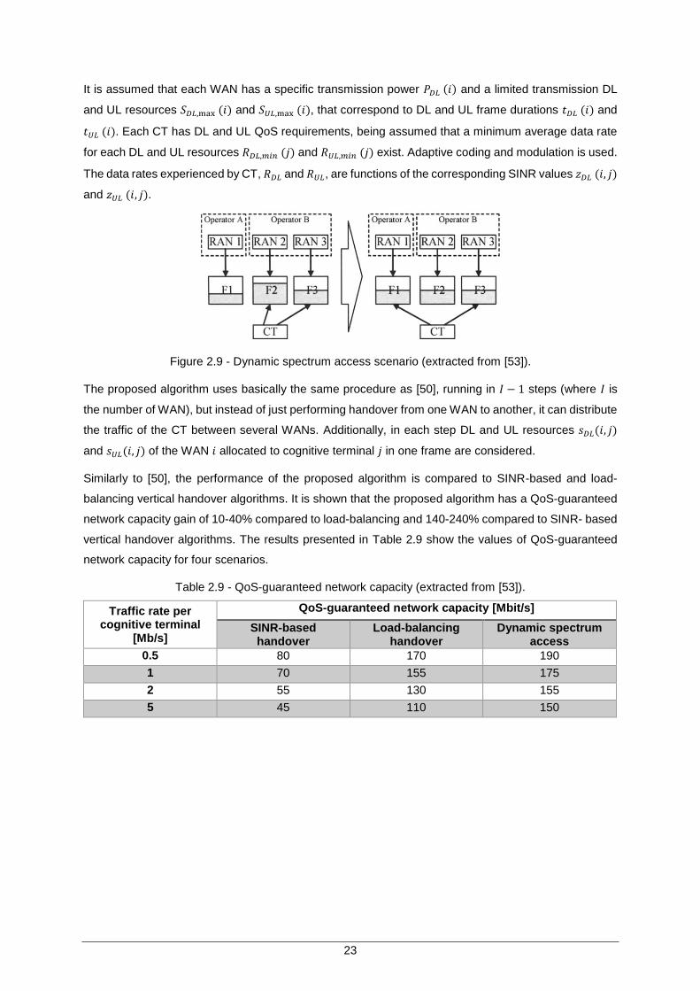
23
It is assumed that each WAN has a specific transmission power 𝑃𝐷𝐿 (𝑖) and a limited transmission DL
and UL resources 𝑆𝐷𝐿,max (𝑖) and 𝑆𝑈𝐿,max (𝑖), that correspond to DL and UL frame durations 𝑡𝐷𝐿 (𝑖) and
𝑡𝑈𝐿 (𝑖). Each CT has DL and UL QoS requirements, being assumed that a minimum average data rate
for each DL and UL resources 𝑅𝐷𝐿,𝑚𝑖𝑛 (𝑗) and 𝑅𝑈𝐿,𝑚𝑖𝑛 (𝑗) exist. Adaptive coding and modulation is used.
The data rates experienced by CT, 𝑅𝐷𝐿 and 𝑅𝑈𝐿, are functions of the corresponding SINR values 𝑧𝐷𝐿 (𝑖, 𝑗)
and 𝑧𝑈𝐿 (𝑖, 𝑗).
Figure 2.9 - Dynamic spectrum access scenario (extracted from [53]).
The proposed algorithm uses basically the same procedure as [50], running in 𝐼 − 1 steps (where 𝐼 is
the number of WAN), but instead of just performing handover from one WAN to another, it can distribute
the traffic of the CT between several WANs. Additionally, in each step DL and UL resources 𝑠𝐷𝐿(𝑖, 𝑗)
and 𝑠𝑈𝐿(𝑖, 𝑗) of the WAN 𝑖 allocated to cognitive terminal 𝑗 in one frame are considered.
Similarly to [50], the performance of the proposed algorithm is compared to SINR-based and load-
balancing vertical handover algorithms. It is shown that the proposed algorithm has a QoS-guaranteed
network capacity gain of 10-40% compared to load-balancing and 140-240% compared to SINR- based
vertical handover algorithms. The results presented in Table 2.9 show the values of QoS-guaranteed
network capacity for four scenarios.
Table 2.9 - QoS-guaranteed network capacity (extracted from [53]).
Traffic rate per cognitive terminal
[Mb/s]
QoS-guaranteed network capacity [Mbit/s]
SINR-based handover
Load-balancing handover
Dynamic spectrum access
0.5 80 170 190
1 70 155 175
2 55 130 155
5 45 110 150

24
25
Chapter 3
Models and Simulator
Description
3 Models and Simulator Description
A description of the models used in this thesis is provided in this chapter, wherein all the mathematical
formulation, algorithms and implementation are detailed. At the end of the chapter, a brief assessment
of the simulator is done.
26
3.1 Model Description
This section provides a description of the model used in this thesis, with its corresponding mathematical
formulation. In order to accomplish a more accurate evaluation of the link and system performances, a
model with realistic propagation characteristics was used. These characteristics are affected by various
parameters, like the carrier frequency, MIMO order, bandwidth, and antenna characteristics, among
others. A hierarchical coverage scenario is implemented, consisting of three carriers operating in
2 600 MHz, 1 800 MHz and 800 MHz, each one having its respective bandwidths. Usually, the closer a
UE is to a BS, the higher throughput it can reach with the same amount of resources. The model
established created in this thesis evaluates the traffic generated by each sector, aims at maximising
capacity by balancing the UEs through HOs for different FBs, always ensuring QoS. It is important to
note that all HOs described in this work are IFHO; intra-frequency HOs were not considered.
In short, the model is separated into three modules. The first one deals with the generation of users,
which takes a given service mix and the population density of different areas of a city into account. In
the second, a network with the city scenario (streets, zones) and BSs with the respective coverage areas
for each FB is deployed. Then, users generated in the first module are inserted into this network, and
the network analysis starts, proceeding to the next module. It calculates the load of each sector by
means of the RBs used for each UE. For overloaded sectors, the model removes RBs to low priority
users until they reach the minimum throughput or are delayed. The available capacity of sectors is
distributed to connected UEs. When the LBIFHO algorithm takes place, some UEs suffer IFHO to an
FB that offers better SNR conditions, spending fewer resources and freeing capacity to other UEs. A
more detailed description of all these steps is presented in the next sections.
The antenna gain influences the results, as it expands or shrinks the coverage area, covering more or
less users, respectively, having also a direct impact on the UE received power and on the SINR.
The equations to calculate the antenna gain are based on [54]; but in this first calculation, it is not
possible yet to determine the users’ distance to the BS, so the coverage area of each sector is calculated
based on a reference throughput, corresponding to a minimum throughput that guarantees QoS for the
service that expends fewer resources, which in this case is voice. UEs are considered to be served if
they reach at least a minimum throughput. Using COST-231 Walfisch-Ikegami Propagation Model ([24],
[10]) presented in Annex A and Annex B, plus the formulation that relates SNR with throughput per RB
given in Annex C, it is possible to calculate the maximum distance 𝑑𝑚𝑎𝑥 that a user can be from the BS
(excluding downtilt and considering maximum antenna gain), by means of the reference throughput.
One should note that the path loss formulation used in this thesis does not take diffraction or scattering
in the near field of the antenna into account (e.g., the mast, or other objects in the vicinity, such as roof-
tops). The antenna radiation patterns defined by (3.1) and (3.2) include some of these effects, [55].
The horizontal pattern of the antenna is given by:
𝐺𝐻[dB](𝜑) = −𝑚𝑖𝑛 [12 (
𝜑[°]
𝜑3dB[°]
)
2
, 𝐴𝑚[dB]] (3.1)

27
where:
𝜑: Angle around the pointing direction of the antenna in the horizontal plane.
𝜑3dB: Horizontal half-power beamwidth.
𝐴𝑚: Front-to-back attenuation.
Due to the omission of the secondary lobe, as shown in Figure 3.1, the front-to-back attenuation must
have a high value.
Figure 3.1 – Layout of horizontal diagram pattern of a tri-sectored antenna.
The vertical radiation pattern of the antenna is given by:
𝐺𝑉[dB] (𝜃) = −𝑚𝑖𝑛 [12 (𝜃[°] − 𝜃𝑒𝑡𝑖𝑙𝑡 [°]
𝜃3dB[°]
)
2
, 𝐴𝑆𝐿[dB]] (3.2)
where:
𝜃: Angle of pointing direction of the antenna in the vertical plane.
𝜃𝑒𝑡𝑖𝑙𝑡: Electrical antenna downtilt.
𝜃3𝑑𝐵: Vertical half-power beamwidth.
𝐴𝑆𝐿: Sidelobe attenuation.
The 𝜓 angle is considered as an average between a user in line of sight (LoS) and Non-LoS conditions,
where the user is assumed to be at the centre of the street, as described in Figure 3.2.
Figure 3.2 – Example of a dense urban scenario (adapted from [24]).
where:
𝜓1[rad]= arctan (
ℎ𝑏[m]−ℎ𝑚[m]
𝑑𝑚𝑎𝑥[m]), LoS (3.3)
𝜓2[rad]= arctan (
ℎ𝑏[m]−𝐻𝐵[m]
𝑑𝑚𝑎𝑥[m]−
𝑤𝑠[m]
2
), Non-LoS (3.4)

28
One can obtain from the previous equations that the 𝜓 angle corresponds to:
𝜓[rad] =𝜓1[rad]
+ 𝜓2[rad]
2 (3.5)
Finally, the total gain of the antenna is given by:
𝐺[dBi](𝜑, 𝜓) = 𝐺𝑚𝑎𝑥[dBi]− min {− [𝐺𝐻[dB]
(𝜑) + 𝐺𝑉[dB] (𝜓)] , 𝐴𝑚[dB]} (3.6)
where:
𝐺𝑚𝑎𝑥: Maximum antenna gain.
With these inputs, it is possible to compute the coverage area by means of redoing the calculations of
the COST 231 Walfisch Ikegami and obtaining the radius that corresponds to each 𝜑 angle.
The expression to calculate throughput, described in Section 2.3, is used in a different way. After
calculating the SNR of a specific user, one can estimate the 𝑅𝑏,𝑅𝐵 using the formulation presented in
Annex C. Then, in a first approach, calculating the amount of 𝑁𝑅𝐵,𝑢𝑠𝑒𝑟 necessary to reach the average
throughput of a given service, it is possible to calculate the UE throughput, given by [30]:
𝑅𝑏,𝑢𝑠𝑒𝑟[Mbit s⁄ ]= ∑ 𝑅𝑏,𝑅𝐵 𝑖 [Mbit s⁄ ]
𝑁𝑅𝐵,𝑢𝑠𝑒𝑟
𝑖=1
(3.7)
where:
𝑁𝑅𝐵,𝑢𝑠𝑒𝑟: Number of RBs allocated to the UE.
𝑅𝑏,𝑅𝐵 𝑖: Throughput of 𝑖𝑡ℎ RB.
The total throughput of a given sector can be obtained from [30]:
𝑅𝑏,𝑠𝑒𝑐𝑡𝑜𝑟[Mbit s⁄ ]= ∑ 𝑅𝑏,𝑢𝑠𝑒𝑟 𝑖 [Mbit s⁄ ]
𝑁𝑢,𝑠𝑒𝑐
𝑖=1
(3.8)
where:
𝑁𝑢,𝑠𝑒𝑐: Number of users served by the sector.
Since the average throughput is an output parameter, it needs to be defined. An example of this is given
in (3.9), in this case corresponding to the average throughput per user of a given service.
𝜇𝑡𝑝𝑢,𝑎=
1
𝑁𝑢,𝑠
∑ 𝑅𝑏,𝑢𝑠𝑒𝑟 𝑖 [Mbit s⁄ ]
𝑁𝑢,𝑠
𝑖=1
(3.9)
where:
𝑁𝑢,𝑠: Number of active users in the service s.
The load factor of a sector is given by:
𝐿𝑠𝑒𝑐𝑡𝑜𝑟[%] =∑ 𝑁𝑅𝐵,𝑢,𝑠𝑒𝑐
𝑁𝑢,𝑠𝑒𝑐
1
𝑁𝑅𝐵,𝑡𝑜𝑡𝑎𝑙,𝑠𝑒𝑐
(3.10)
where:
𝑁𝑅𝐵,𝑢,𝑠𝑒𝑐: Number of used RB per user in a given sector.
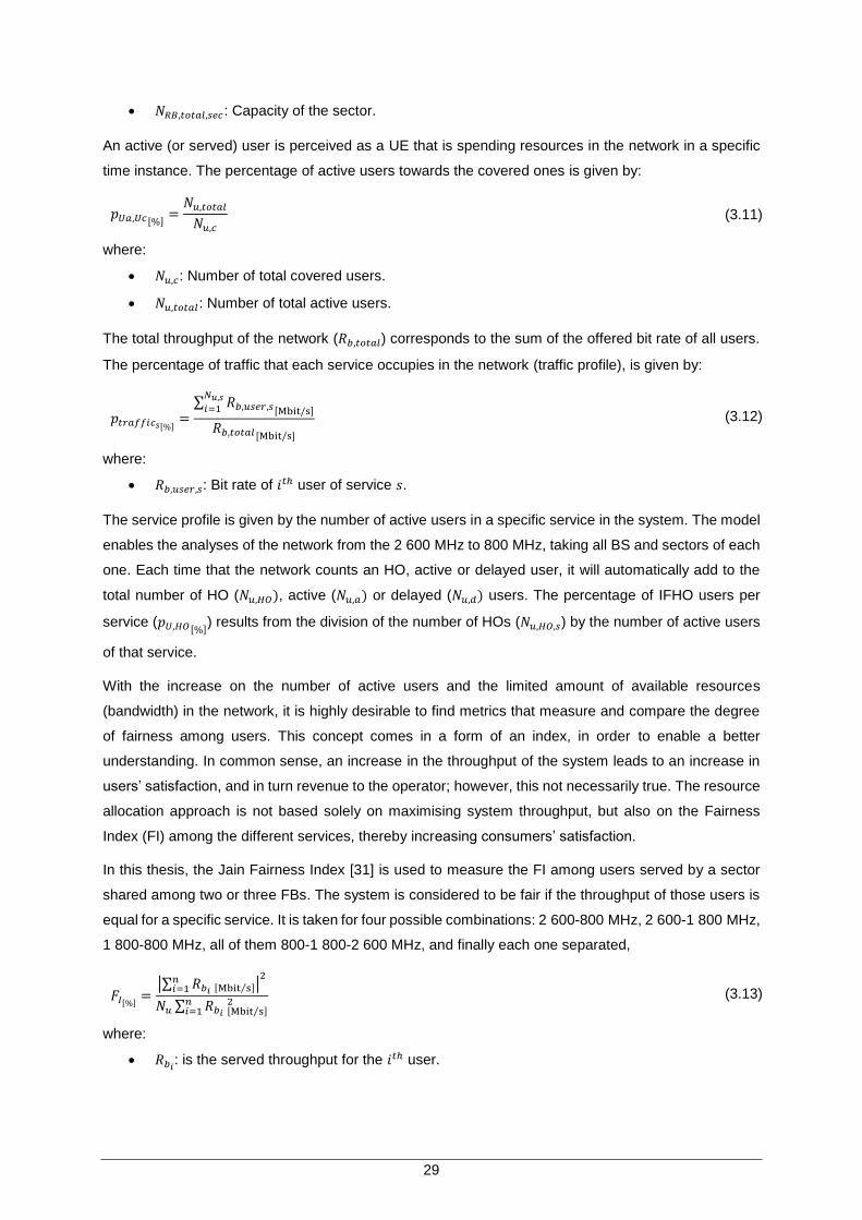
29
𝑁𝑅𝐵,𝑡𝑜𝑡𝑎𝑙,𝑠𝑒𝑐: Capacity of the sector.
An active (or served) user is perceived as a UE that is spending resources in the network in a specific
time instance. The percentage of active users towards the covered ones is given by:
𝑝𝑈𝑎,𝑈𝑐[%]=
𝑁𝑢,𝑡𝑜𝑡𝑎𝑙
𝑁𝑢,𝑐
(3.11)
where:
𝑁𝑢,𝑐: Number of total covered users.
𝑁𝑢,𝑡𝑜𝑡𝑎𝑙: Number of total active users.
The total throughput of the network (𝑅𝑏,𝑡𝑜𝑡𝑎𝑙) corresponds to the sum of the offered bit rate of all users.
The percentage of traffic that each service occupies in the network (traffic profile), is given by:
𝑝𝑡𝑟𝑎𝑓𝑓𝑖𝑐𝑠[%]=
∑ 𝑅𝑏,𝑢𝑠𝑒𝑟,𝑠𝑁𝑢,𝑠
𝑖=1 [Mbit/s]
𝑅𝑏,𝑡𝑜𝑡𝑎𝑙 [Mbit/s]
(3.12)
where:
𝑅𝑏,𝑢𝑠𝑒𝑟,𝑠: Bit rate of 𝑖𝑡ℎ user of service 𝑠.
The service profile is given by the number of active users in a specific service in the system. The model
enables the analyses of the network from the 2 600 MHz to 800 MHz, taking all BS and sectors of each
one. Each time that the network counts an HO, active or delayed user, it will automatically add to the
total number of HO (𝑁𝑢,𝐻𝑂), active (𝑁𝑢,𝑎) or delayed (𝑁𝑢,𝑑) users. The percentage of IFHO users per
service (𝑝𝑈,𝐻𝑂[%]) results from the division of the number of HOs (𝑁𝑢,𝐻𝑂,𝑠) by the number of active users
of that service.
With the increase on the number of active users and the limited amount of available resources
(bandwidth) in the network, it is highly desirable to find metrics that measure and compare the degree
of fairness among users. This concept comes in a form of an index, in order to enable a better
understanding. In common sense, an increase in the throughput of the system leads to an increase in
users’ satisfaction, and in turn revenue to the operator; however, this not necessarily true. The resource
allocation approach is not based solely on maximising system throughput, but also on the Fairness
Index (FI) among the different services, thereby increasing consumers’ satisfaction.
In this thesis, the Jain Fairness Index [31] is used to measure the FI among users served by a sector
shared among two or three FBs. The system is considered to be fair if the throughput of those users is
equal for a specific service. It is taken for four possible combinations: 2 600-800 MHz, 2 600-1 800 MHz,
1 800-800 MHz, all of them 800-1 800-2 600 MHz, and finally each one separated,
where:
𝑅𝑏𝑖: is the served throughput for the 𝑖𝑡ℎ user.
𝐹𝐼[%]=
|∑ 𝑅𝑏𝑖 [Mbit s⁄ ]
𝑛𝑖=1 |
2
𝑁𝑢 ∑ 𝑅𝑏𝑖 [Mbit s⁄ ]2𝑛
𝑖=1
(3.13)
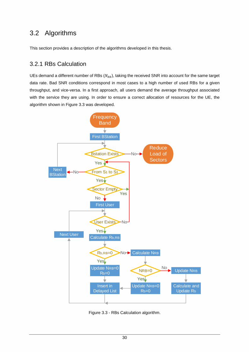
30
3.2 Algorithms
This section provides a description of the algorithms developed in this thesis.
3.2.1 RBs Calculation
UEs demand a different number of RBs (𝑁𝑅𝐵), taking the received SNR into account for the same target
data rate. Bad SNR conditions correspond in most cases to a high number of used RBs for a given
throughput, and vice-versa. In a first approach, all users demand the average throughput associated
with the service they are using. In order to ensure a correct allocation of resources for the UE, the
algorithm shown in Figure 3.3 was developed.
Frequency
Band
First BStation
Bstation Exists
Reduce
Load of
Sectors
Next
BStationFrom S1 to S3
First User
Sector Empty
User Exists
Calculate Rb,RB
Rb,RB=0 Calculate NRB
NRB=0Update NRB=0
Rb=0
Update NRB=0
Rb=0
Update NRB
Calculate and
Update Rb
Insert in
Delayed List
Next User
Yes
Yes
No
No
No
Yes
No
No
Yes
Yes
Yes
No
Figure 3.3 - RBs Calculation algorithm.
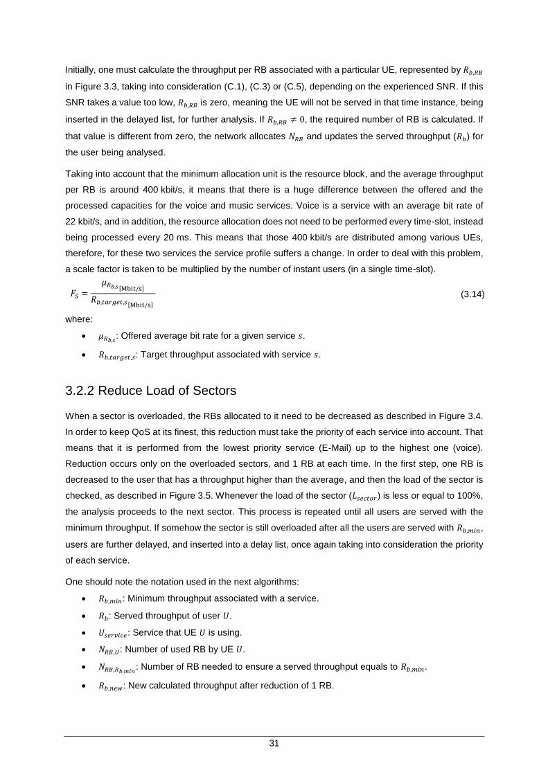
31
Initially, one must calculate the throughput per RB associated with a particular UE, represented by 𝑅𝑏,𝑅𝐵
in Figure 3.3, taking into consideration (C.1), (C.3) or (C.5), depending on the experienced SNR. If this
SNR takes a value too low, 𝑅𝑏,𝑅𝐵 is zero, meaning the UE will not be served in that time instance, being
inserted in the delayed list, for further analysis. If 𝑅𝑏,𝑅𝐵 ≠ 0, the required number of RB is calculated. If
that value is different from zero, the network allocates 𝑁𝑅𝐵 and updates the served throughput (𝑅𝑏) for
the user being analysed.
Taking into account that the minimum allocation unit is the resource block, and the average throughput
per RB is around 400 kbit/s, it means that there is a huge difference between the offered and the
processed capacities for the voice and music services. Voice is a service with an average bit rate of
22 kbit/s, and in addition, the resource allocation does not need to be performed every time-slot, instead
being processed every 20 ms. This means that those 400 kbit/s are distributed among various UEs,
therefore, for these two services the service profile suffers a change. In order to deal with this problem,
a scale factor is taken to be multiplied by the number of instant users (in a single time-slot).
𝐹𝑆 =𝜇𝑅𝑏,𝑠[Mbit/s]
𝑅𝑏,𝑡𝑎𝑟𝑔𝑒𝑡,𝑠[Mbit/s] (3.14)
where:
𝜇𝑅𝑏,𝑠: Offered average bit rate for a given service 𝑠.
𝑅𝑏,𝑡𝑎𝑟𝑔𝑒𝑡,𝑠: Target throughput associated with service 𝑠.
3.2.2 Reduce Load of Sectors
When a sector is overloaded, the RBs allocated to it need to be decreased as described in Figure 3.4.
In order to keep QoS at its finest, this reduction must take the priority of each service into account. That
means that it is performed from the lowest priority service (E-Mail) up to the highest one (voice).
Reduction occurs only on the overloaded sectors, and 1 RB at each time. In the first step, one RB is
decreased to the user that has a throughput higher than the average, and then the load of the sector is
checked, as described in Figure 3.5. Whenever the load of the sector (𝐿𝑠𝑒𝑐𝑡𝑜𝑟) is less or equal to 100%,
the analysis proceeds to the next sector. This process is repeated until all users are served with the
minimum throughput. If somehow the sector is still overloaded after all the users are served with 𝑅𝑏,𝑚𝑖𝑛,
users are further delayed, and inserted into a delay list, once again taking into consideration the priority
of each service.
One should note the notation used in the next algorithms:
𝑅𝑏,𝑚𝑖𝑛: Minimum throughput associated with a service.
𝑅𝑏: Served throughput of user 𝑈.
𝑈𝑠𝑒𝑟𝑣𝑖𝑐𝑒: Service that UE 𝑈 is using.
𝑁𝑅𝐵,𝑈: Number of used RB by UE 𝑈.
𝑁𝑅𝐵,𝑅𝑏,𝑚𝑖𝑛: Number of RB needed to ensure a served throughput equals to 𝑅𝑏,𝑚𝑖𝑛.
𝑅𝑏,𝑛𝑒𝑤: New calculated throughput after reduction of 1 RB.
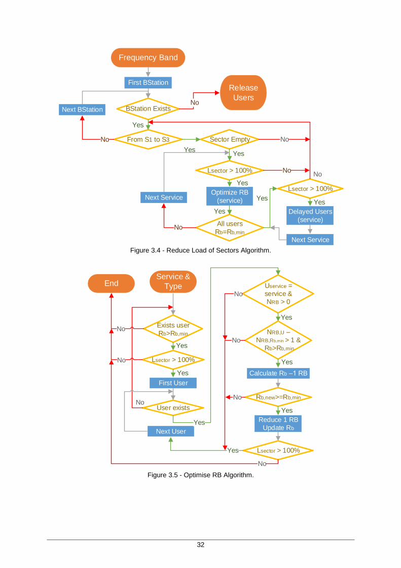
32
Frequency Band
First BStation
BStation Exists
Release
Users
Next BStation
From S1 to S3 Sector Empty
Yes
No
No
Lsector > 100%
Optimize RB
(service)
All users
Rb=Rb,min
Next Service
Lsector > 100%
Next Service
Delayed Users
(service)
Yes
Yes
No
No
No
Yes
Yes
Yes
Yes
No
Figure 3.4 - Reduce Load of Sectors Algorithm.
Exists user
Rb>Rb,min
Lsector > 100%
User exists
Uservice =
service &
NRB > 0
NRB,U –
NRB,Rb,min > 1 &
Rb>Rb,min
Rb,new>=Rb,min
Lsector > 100%
First User
Yes
Yes
Yes
Service &
TypeEnd
Calculate Rb – RB
Reduce 1 RB
Update Rb
Yes
Yes
Next User
No
No
No
No
Yes
No
No
No
Yes
Figure 3.5 - Optimise RB Algorithm.
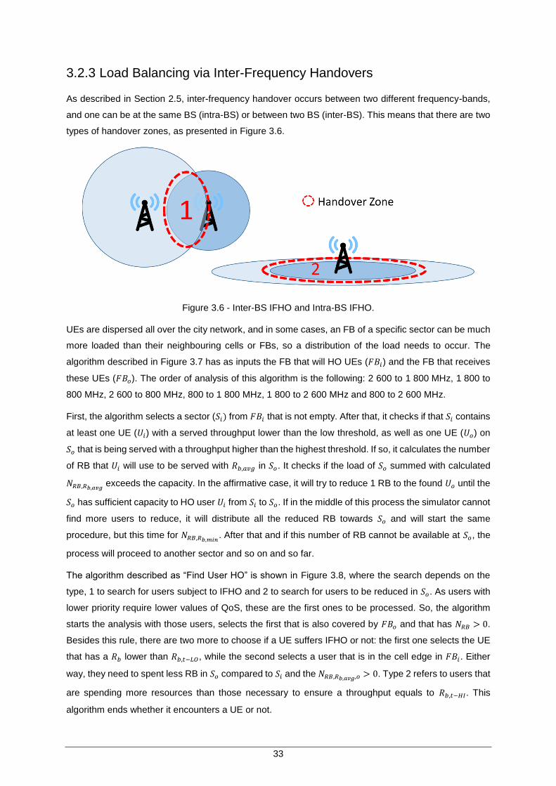
33
3.2.3 Load Balancing via Inter-Frequency Handovers
As described in Section 2.5, inter-frequency handover occurs between two different frequency-bands,
and one can be at the same BS (intra-BS) or between two BS (inter-BS). This means that there are two
types of handover zones, as presented in Figure 3.6.
Figure 3.6 - Inter-BS IFHO and Intra-BS IFHO.
UEs are dispersed all over the city network, and in some cases, an FB of a specific sector can be much
more loaded than their neighbouring cells or FBs, so a distribution of the load needs to occur. The
algorithm described in Figure 3.7 has as inputs the FB that will HO UEs (𝐹𝐵𝑖) and the FB that receives
these UEs (𝐹𝐵𝑜). The order of analysis of this algorithm is the following: 2 600 to 1 800 MHz, 1 800 to
800 MHz, 2 600 to 800 MHz, 800 to 1 800 MHz, 1 800 to 2 600 MHz and 800 to 2 600 MHz.
First, the algorithm selects a sector (𝑆𝑖) from 𝐹𝐵𝑖 that is not empty. After that, it checks if that 𝑆𝑖 contains
at least one UE (𝑈𝑖) with a served throughput lower than the low threshold, as well as one UE (𝑈𝑜) on
𝑆𝑜 that is being served with a throughput higher than the highest threshold. If so, it calculates the number
of RB that 𝑈𝑖 will use to be served with 𝑅𝑏,𝑎𝑣𝑔 in 𝑆𝑜. It checks if the load of 𝑆𝑜 summed with calculated
𝑁𝑅𝐵,𝑅𝑏,𝑎𝑣𝑔 exceeds the capacity. In the affirmative case, it will try to reduce 1 RB to the found 𝑈𝑜 until the
𝑆𝑜 has sufficient capacity to HO user 𝑈𝑖 from 𝑆𝑖 to 𝑆𝑜. If in the middle of this process the simulator cannot
find more users to reduce, it will distribute all the reduced RB towards 𝑆𝑜 and will start the same
procedure, but this time for 𝑁𝑅𝐵,𝑅𝑏,𝑚𝑖𝑛. After that and if this number of RB cannot be available at 𝑆𝑜, the
process will proceed to another sector and so on and so far.
The algorithm described as “Find User HO” is shown in Figure 3.8, where the search depends on the
type, 1 to search for users subject to IFHO and 2 to search for users to be reduced in 𝑆𝑜. As users with
lower priority require lower values of QoS, these are the first ones to be processed. So, the algorithm
starts the analysis with those users, selects the first that is also covered by 𝐹𝐵𝑜 and that has 𝑁𝑅𝐵 > 0.
Besides this rule, there are two more to choose if a UE suffers IFHO or not: the first one selects the UE
that has a 𝑅𝑏 lower than 𝑅𝑏,𝑡−𝐿𝑂, while the second selects a user that is in the cell edge in 𝐹𝐵𝑖. Either
way, they need to spent less RB in 𝑆𝑜 compared to 𝑆𝑖 and the 𝑁𝑅𝐵,𝑅𝑏,𝑎𝑣𝑔,𝑜 > 0. Type 2 refers to users that
are spending more resources than those necessary to ensure a throughput equals to 𝑅𝑏,𝑡−𝐻𝐼. This
algorithm ends whether it encounters a UE or not.
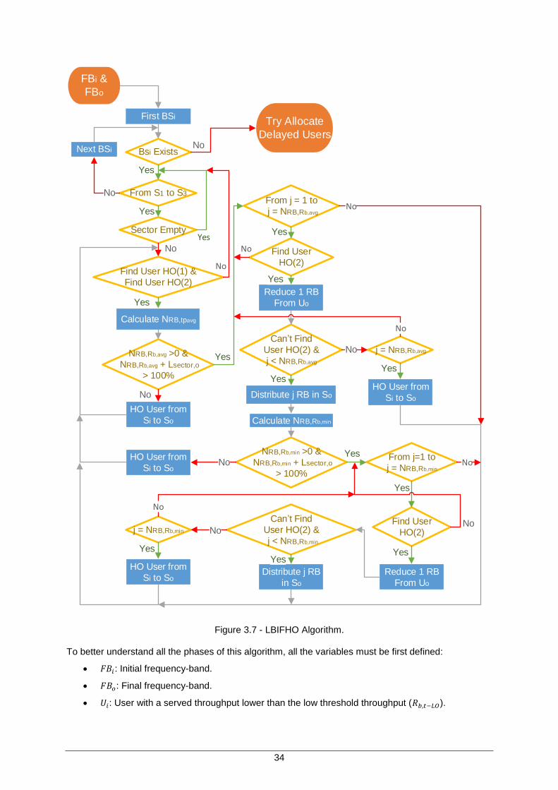
34
FBi &
FBo
First BSi
From S1 to S3
Bsi Exists
Sector Empty
Find User HO(1) &
Find User HO(2)
Calculate NRB,tpavg
NRB,Rb,avg >0 &
NRB,Rb,avg + Lsector,o
> 100%
HO User from
Si to So
Find User
HO(2)
From j = 1 to
j = NRB,Rb,avg
Can t Find
User HO(2) &
j < NRB,Rb,avg
Distribute j RB in So
j = NRB,Rb,avg
HO User from
Si to So
Yes
Yes
No
Yes
No
Yes
Reduce 1 RB
From Uo
No
Yes
Yes
YesYes
Try Allocate
Delayed UsersNoNext BSi
No
NRB,Rb,min >0 &
NRB,Rb,min + Lsector,o
> 100%
HO User from
Si to So
Find User
HO(2)
From j=1 to
j = NRB,Rb,min
Can t Find
User HO(2) &
j < NRB,Rb,min
Distribute j RB
in So
j = NRB,Rb,min
HO User from
Si to SoReduce 1 RB
From Uo
YesNo
No
YesYes
Yes
Yes
Calculate NRB,Rb,min
No
No
No
No
Yes
No
No
No
Figure 3.7 - LBIFHO Algorithm.
To better understand all the phases of this algorithm, all the variables must be first defined:
𝐹𝐵𝑖: Initial frequency-band.
𝐹𝐵𝑜: Final frequency-band.
𝑈𝑖: User with a served throughput lower than the low threshold throughput (𝑅𝑏,𝑡−𝐿𝑂).
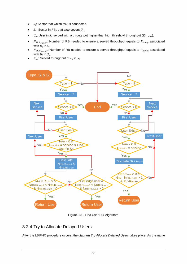
35
𝑆𝑖: Sector that which 𝑈𝐸𝑖 is connected.
𝑆𝑜: Sector in 𝐹𝐵𝑜 that also covers 𝑈𝑖.
𝑈𝑜: User in 𝑆𝑜 served with a throughput higher than high threshold throughput (𝑅𝑏,𝑡−𝐻𝐼).
𝑁𝑅𝐵,𝑅𝑏,𝑎𝑣𝑔,𝑖: Number of RB needed to ensure a served throughput equals to 𝑅𝑏,𝑎𝑣𝑔 associated
with 𝑈𝑖 in 𝑆𝑖.
𝑁𝑅𝐵,𝑅𝑏,𝑎𝑣𝑔,𝑜: Number of RB needed to ensure a served throughput equals to 𝑅𝑏,𝑚𝑖𝑛 associated
with 𝑈𝑖 in 𝑆𝑜.
𝑅𝑏,𝑖: Served throughput of 𝑈𝑖 in 𝑆𝑖.
Type, Si & So
Next User
First User
Type = 2Type = 1
User Exists
NRB > 0 &
Uservice = service
Service = 7
Service = 0
Calculate NRB,Rb,t-HI
NRB,Rb,t-HI > 0 &
NRB - NRB,Rb,t-HI > 1
& Rb>Rb,t-HI
Return User
Next
Service
Next User
First User
User Exists
NRB > 0 &
Uservice = service & Find
User in So
Service = 7
Service = 0
Calculate
NRB,Rb,avg,i &
NRB,Rb,avg,o
Rb,i < Rb,t-LO &
NRB,Rb,avg,o < NRB,Rb,avg,i
& NRB,Rb,avg,o > 0
Cell edge user &
NRB,Rb,avg,o < NRB,Rb,avg,i
& NRB,Rb,avg,o > 0
Return UserReturn User
Yes
No
Yes
No
Yes
No
Yes
YesYes
No
Yes
Yes
Yes
EndYes Yes
No
No
Next
Service
No
No
No
No
No
Figure 3.8 - Find User HO Algorithm.
3.2.4 Try to Allocate Delayed Users
After the LBIFHO procedure occurs, the diagram Try Allocate Delayed Users takes place. As the name
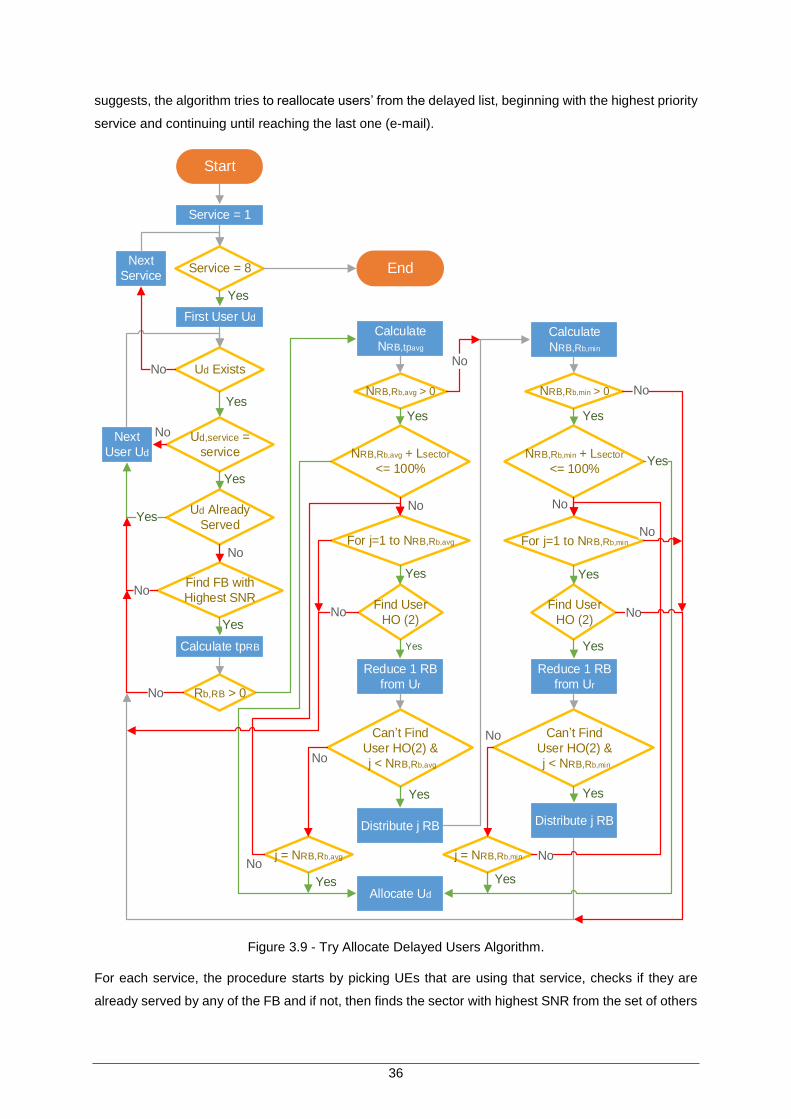
36
suggests, the algorithm tries to reallocate users’ from the delayed list, beginning with the highest priority
service and continuing until reaching the last one (e-mail).
EndService = 8
First User Ud
Ud,service =
service
Ud Already
Served
Find FB with
Highest SNR
Calculate tpRB
Rb,RB > 0
Calculate
NRB,tpavg
NRB,Rb,avg + Lsector
<= 100%
For j=1 to NRB,Rb,avg
Reduce 1 RB
from Ur
Find User
HO (2)
Can t Find
User HO(2) &
j < NRB,Rb,avg
Distribute j RB
j = NRB,Rb,avg
Allocate Ud
Service = 1
Calculate
NRB,Rb,min
NRB,Rb,min + Lsector
<= 100%
For j=1 to NRB,Rb,min
Reduce 1 RB
from Ur
Find User
HO (2)
Can t Find
User HO(2) &
j < NRB,Rb,min
Distribute j RB
j = NRB,Rb,min
Next
User Ud
Next
Service
Ud Exists
Start
Yes
Yes
Yes
No
Yes
No
Yes
Yes
Yes
No
Yes
Yes
Yes
No
No
Yes
No
No
No
Yes
No
No
NRB,Rb,min > 0NRB,Rb,avg > 0
Yes Yes
No
No
No
Yes Yes
No
No
No
Figure 3.9 - Try Allocate Delayed Users Algorithm.
For each service, the procedure starts by picking UEs that are using that service, checks if they are
already served by any of the FB and if not, then finds the sector with highest SNR from the set of others
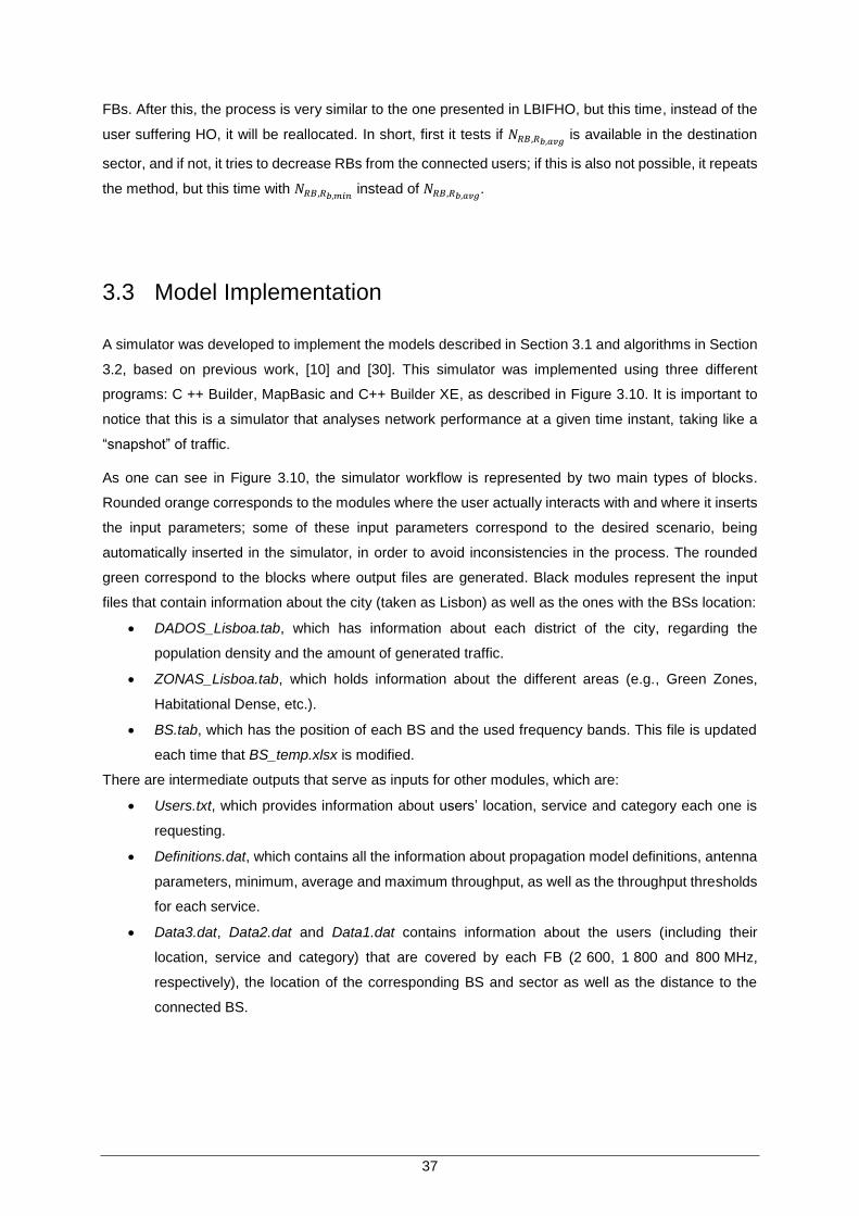
37
FBs. After this, the process is very similar to the one presented in LBIFHO, but this time, instead of the
user suffering HO, it will be reallocated. In short, first it tests if 𝑁𝑅𝐵,𝑅𝑏,𝑎𝑣𝑔 is available in the destination
sector, and if not, it tries to decrease RBs from the connected users; if this is also not possible, it repeats
the method, but this time with 𝑁𝑅𝐵,𝑅𝑏,𝑚𝑖𝑛 instead of 𝑁𝑅𝐵,𝑅𝑏,𝑎𝑣𝑔
.
3.3 Model Implementation
A simulator was developed to implement the models described in Section 3.1 and algorithms in Section
3.2, based on previous work, [10] and [30]. This simulator was implemented using three different
programs: C ++ Builder, MapBasic and C++ Builder XE, as described in Figure 3.10. It is important to
notice that this is a simulator that analyses network performance at a given time instant, taking like a
“snapshot” of traffic.
As one can see in Figure 3.10, the simulator workflow is represented by two main types of blocks.
Rounded orange corresponds to the modules where the user actually interacts with and where it inserts
the input parameters; some of these input parameters correspond to the desired scenario, being
automatically inserted in the simulator, in order to avoid inconsistencies in the process. The rounded
green correspond to the blocks where output files are generated. Black modules represent the input
files that contain information about the city (taken as Lisbon) as well as the ones with the BSs location:
DADOS_Lisboa.tab, which has information about each district of the city, regarding the
population density and the amount of generated traffic.
ZONAS_Lisboa.tab, which holds information about the different areas (e.g., Green Zones,
Habitational Dense, etc.).
BS.tab, which has the position of each BS and the used frequency bands. This file is updated
each time that BS_temp.xlsx is modified.
There are intermediate outputs that serve as inputs for other modules, which are:
Users.txt, which provides information about users’ location, service and category each one is
requesting.
Definitions.dat, which contains all the information about propagation model definitions, antenna
parameters, minimum, average and maximum throughput, as well as the throughput thresholds
for each service.
Data3.dat, Data2.dat and Data1.dat contains information about the users (including their
location, service and category) that are covered by each FB (2 600, 1 800 and 800 MHz,
respectively), the location of the corresponding BS and sector as well as the distance to the
connected BS.
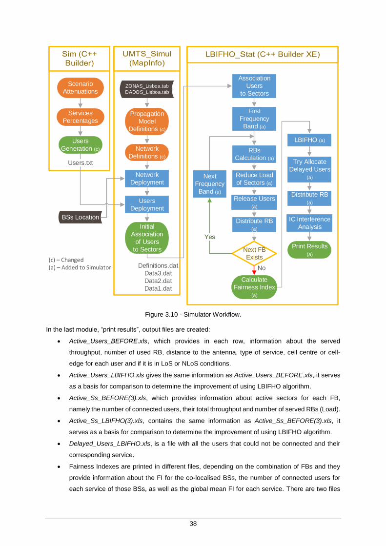
38
Association
Users
to Sectors
RBs
Calculation (a)
Reduce Load
of Sectors (a)
Release Users
(a)
Distribute RB
(a)
Calculate
Fairness Index
(a)
Print Results
(a)
Next
Frequency
Band (a)
Next FB
Exists
Yes
No
First
Frequency
Band (a)
LBIFHO (a)
Try Allocate
Delayed Users
(a)
Distribute RB
(a)
IC Interference
Analysis
Propagation
Model
Definitions (c)
Network
Deployment
Users
Deployment
Network
Definitions (c)
Initial
Association
of Users
to Sectors
Scenario
Attenuations
Users
Generation (c)
Services
Percentages
BSs Location
Definitions.dat
Data3.dat
Data2.dat
Data1.dat
Users.txt
ZONAS_Lisboa.tab
DADOS_Lisboa.tab
(c) – Changed(a) – Added to Simulator
Figure 3.10 - Simulator Workflow.
In the last module, “print results”, output files are created:
Active_Users_BEFORE.xls, which provides in each row, information about the served
throughput, number of used RB, distance to the antenna, type of service, cell centre or cell-
edge for each user and if it is in LoS or NLoS conditions.
Active_Users_LBIFHO.xls gives the same information as Active_Users_BEFORE.xls, it serves
as a basis for comparison to determine the improvement of using LBIFHO algorithm.
Active_Ss_BEFORE(3).xls, which provides information about active sectors for each FB,
namely the number of connected users, their total throughput and number of served RBs (Load).
Active_Ss_LBIFHO(3).xls, contains the same information as Active_Ss_BEFORE(3).xls, it
serves as a basis for comparison to determine the improvement of using LBIFHO algorithm.
Delayed_Users_LBIFHO.xls, is a file with all the users that could not be connected and their
corresponding service.
Fairness Indexes are printed in different files, depending on the combination of FBs and they
provide information about the FI for the co-localised BSs, the number of connected users for
each service of those BSs, as well as the global mean FI for each service. There are two files
39
for each combination, one for before and other for after the LBIFHO occurs.
Stats(3).txt, has information about the average UE, sector and BS throughput as well as the
number of used RBs. It also gives the number of covered and active users for a given service,
average centre and border users’ throughput. The (3) represent three files, one for each FB.
StatsLBIFHO.txt, is similar to Stats.txt, but instead of analysing one FB, it has the result for the
entire network, after the LBIFHO algorithm has been executed. Gives the percentage of active
users towards the covered ones, the number of users that have 𝑅𝑏𝑅𝐵= 0, as well as the total
number of HOs, delayed, reallocated and HO users.
The first phase of this simulator deals with user generation, creating a .txt file that includes the users
positioning along the city, as well as information about the service that each user is requesting, based
on the defined services percentages. It is important to note that the user category is a parameter
implemented in this module, varying between category 3 and 5, enabling a more realistic approach.
Users distribution takes real population density for each zone of the city, but it has an approximation:
this distribution occurs in squares, causing approximately 10% of the total users to be outside the
boundaries of the city, and consequently not covered.
Then the user needs to run UMTS_Simul.mbx in order to continue the simulation. The name given to
this module comes from the previous work that dealt with 3G systems, and because it has the possibility
to run any of them. The user’s manual with the proceedings for the execution of this module presented
in Annex D. After the insertion of all antenna parameters, propagation model and BSs location, the
coverage area for each one of the frequency bands is calculated. This coverage is based on a reference
throughput, which corresponds to the minimum throughput to guarantee the QoS for the service that
expends fewer resources, which in this case is voice (5 kbit/s). After that, a certain SNR is calculated
using the expressions given in Annex C using QPSK, because it is the most reliable modulation for low
SNR conditions. Taking noise power into account, the calculated SNR is translated into a minimum
received power, and then using the COST 231 - Walfisch-Ikegami model presented in Annex B, Annex
A and the equations in Section 3.1, the sector radius for each FB is extracted. After the calculation and
representation of all sectors, the users file previously generated in the first module is inserted. UEs are
deployed in the network, and the final block ensures a first association of users to sectors based on
whether they are located inside the coverage area of a given sector or not. This first approach associates
a user to all the sectors that is covered by; since there are various overlapping coverage areas, a user
can be connected to more than one sector.
After this association, MapInfo automatically calls LBIFHO_Stats.exe. The first block in this module
reads the information generated by MapInfo saving their information in data structures. A more careful
examination is done, where users are connected to the sector that offers them the greatest SNR. In the
interest of efficiency and simplicity, this association is executed separately for each FB.
At this moment, all users are distributed regarding the best SNR conditions, and RBs are allocated
taking the throughput each user requires into account. In a first approach, it corresponds to the average
throughput defined by some input parameters. As the highest frequency band (2 600 MHz) has the
highest available capacity, it is also the first one to be treated. The algorithm used for this calculation is
40
described in Figure 3.3.
Taking into account the different population density of the districts of a city, some sectors can be
overcharged, meaning that a reduction has to occur, in order to be coherent with system capacity. This
reduction is carried out by the algorithm described in Figure 3.4, where in a first approach, the throughput
of each UE is decreased until it reaches a minimum throughput, or the capacity limit is achieved. Users
served by one FB do not need to be analysed in the others. This process is treated by the Release
Users block.
After the calculation of RB and the releasing of users, some sectors may have available RBs that can
be distributed to connected UEs. Once again, they are distributed taking the priorities of services into
account, initially allocating RBs to voice users until all of those are served with 𝑅𝑏𝑚𝑎𝑥, and continuing
the same procedure to other services until the capacity of each sector is completely used.
At this time, all sectors are in their capacity limits, but the load is not corrected distributed, with some
UEs that if connected to other FB could expend fewer resources. If these UEs suffers HO to an FB that
offers them more attractive SNR conditions, the resources allocated to the initial sector will be released.
If implemented on a large scale, it means that more resources will be available to other connected UEs
of that sector, or even enabling reconnection of previously delayed UEs and consequently increasing
the overall capacity of the system. This commonly applies to users at cell edge of higher FBs.
Finally, the algorithm Try Allocate Delayed Users will take place, and as the name suggests, this
algorithm checks if it can reallocate any of the delayed users in the network. The UEs using higher
priority services are the first to be analysed. At the end of the simulation, Distribute RB takes place again
to ensure that there is no sector without all the possible resources allocated. IC Interference Analysis is
the same algorithm as the one proposed in [10], and it was not changed. One should note that IC
Interference Analysis is available in the simulator, but as the interference analysis was out of the scope
of the thesis, it was decided to keep it turned off.
3.4 Model Assessment
In order to ensure the proper functioning of the simulator, a set of tests was considered before
proceeding to the results analysis. The results of the simulation were saved in Microsoft Excel files,
which enabled a more efficient validation of some tests, such as the percentage of active users and the
percentage of generated traffic per service. Table 3.1 describes the most critical tests for the validation
of the simulator.
As previously discussed, the number of covered users does not correspond to the total number of users
generated in the network. This happens for two reasons; 10% of users are positioned outside of city
boundaries by the users’ generation module, and around more 10% other users are positioned outside
the coverage area. This means that the simulator has a coverage efficiency of 80%, e.g., if users’ module
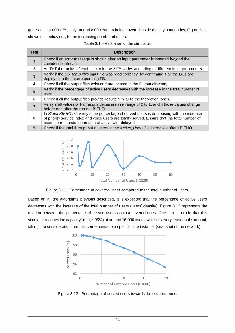
41
generates 10 000 UEs, only around 8 000 end up being covered inside the city boundaries; Figure 3.11
shows this behaviour, for an increasing number of users.
Table 3.1 – Validation of the simulator.
Test Description
1 Check if an error message is shown after an input parameter is inserted beyond the confidence interval.
2 Verify if the radius of each sector in the 3 FB varies according to different input parameters
3 Verify if the BS_temp.xlxs input file was read correctly, by confirming if all the BSs are deployed in their corresponding FB.
4 Check if all the output files exist and are located in the Output directory.
5 Verify if the percentage of active users decreases with the increase in the total number of users.
6 Check if all the output files provide results similar to the theoretical ones.
7 Verify if all values of Fairness Indexes are in a range of 0 to 1, and if those values change before and after the run of LBIFHO.
8 In StatsLBIFHO.txt, verify if the percentage of served users is decreasing with the increase of priority service index and voice users are totally served. Ensure that the total number of users corresponds to the sum of active with delayed.
9 Check if the total throughput of users in the Active_Users file increases after LBIFHO.
Figure 3.11 - Percentage of covered users compared to the total number of users.
Based on all the algorithms previous described, it is expected that the percentage of active users
decreases with the increase of the total number of users (users’ density). Figure 3.12 represents the
relation between the percentage of served users against covered ones. One can conclude that this
simulator reaches the capacity limit (≅ 95%) at around 16 000 users, which is a very reasonable amount,
taking into consideration that this corresponds to a specific time instance (snapshot of the network).
Figure 3.12 - Percentage of served users towards the covered ones.
78.2
78.4
78.6
78.8
79.0
79.2
0 10 20 30 40 50 60
Co
vere
d U
sers
[%
]
Total Number of Users (×1000)
92
94
96
98
100
0 5 10 15 20
Serv
ed U
sers
[%
]
Number of Covered Users (×1000)
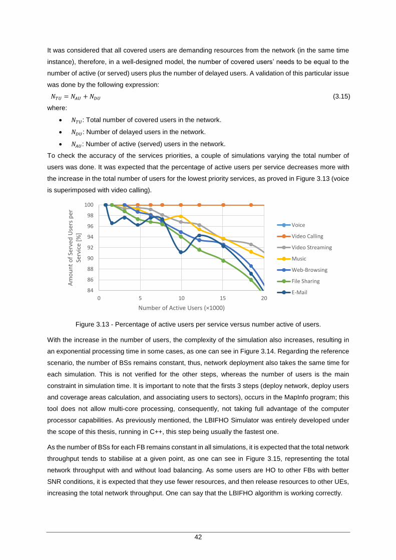
42
It was considered that all covered users are demanding resources from the network (in the same time
instance), therefore, in a well-designed model, the number of covered users’ needs to be equal to the
number of active (or served) users plus the number of delayed users. A validation of this particular issue
was done by the following expression:
𝑁𝑇𝑈 = 𝑁𝐴𝑈 + 𝑁𝐷𝑈 (3.15)
where:
𝑁𝑇𝑈: Total number of covered users in the network.
𝑁𝐷𝑈: Number of delayed users in the network.
𝑁𝐴𝑈: Number of active (served) users in the network.
To check the accuracy of the services priorities, a couple of simulations varying the total number of
users was done. It was expected that the percentage of active users per service decreases more with
the increase in the total number of users for the lowest priority services, as proved in Figure 3.13 (voice
is superimposed with video calling).
Figure 3.13 - Percentage of active users per service versus number active of users.
With the increase in the number of users, the complexity of the simulation also increases, resulting in
an exponential processing time in some cases, as one can see in Figure 3.14. Regarding the reference
scenario, the number of BSs remains constant, thus, network deployment also takes the same time for
each simulation. This is not verified for the other steps, whereas the number of users is the main
constraint in simulation time. It is important to note that the firsts 3 steps (deploy network, deploy users
and coverage areas calculation, and associating users to sectors), occurs in the MapInfo program; this
tool does not allow multi-core processing, consequently, not taking full advantage of the computer
processor capabilities. As previously mentioned, the LBIFHO Simulator was entirely developed under
the scope of this thesis, running in C++, this step being usually the fastest one.
As the number of BSs for each FB remains constant in all simulations, it is expected that the total network
throughput tends to stabilise at a given point, as one can see in Figure 3.15, representing the total
network throughput with and without load balancing. As some users are HO to other FBs with better
SNR conditions, it is expected that they use fewer resources, and then release resources to other UEs,
increasing the total network throughput. One can say that the LBIFHO algorithm is working correctly.
84
86
88
90
92
94
96
98
100
0 5 10 15 20
Am
ou
nt
of
Serv
ed U
sers
per
Se
rvic
e [%
]
Number of Active Users (×1000)
Voice
Video Calling
Video Streaming
Music
Web-Browsing
File Sharing
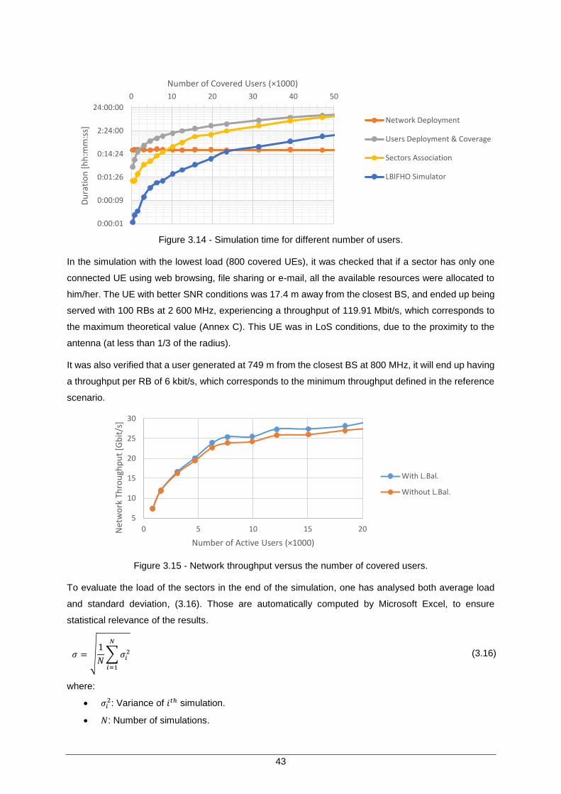
43
Figure 3.14 - Simulation time for different number of users.
In the simulation with the lowest load (800 covered UEs), it was checked that if a sector has only one
connected UE using web browsing, file sharing or e-mail, all the available resources were allocated to
him/her. The UE with better SNR conditions was 17.4 m away from the closest BS, and ended up being
served with 100 RBs at 2 600 MHz, experiencing a throughput of 119.91 Mbit/s, which corresponds to
the maximum theoretical value (Annex C). This UE was in LoS conditions, due to the proximity to the
antenna (at less than 1/3 of the radius).
It was also verified that a user generated at 749 m from the closest BS at 800 MHz, it will end up having
a throughput per RB of 6 kbit/s, which corresponds to the minimum throughput defined in the reference
scenario.
Figure 3.15 - Network throughput versus the number of covered users.
To evaluate the load of the sectors in the end of the simulation, one has analysed both average load
and standard deviation, (3.16). Those are automatically computed by Microsoft Excel, to ensure
statistical relevance of the results.
𝜎 = √1
𝑁∑ 𝜎𝑖
2
𝑁
𝑖=1
(3.16)
where:
𝜎𝑖2: Variance of 𝑖𝑡ℎ simulation.
𝑁: Number of simulations.
0:00:01
0:00:09
0:01:26
0:14:24
2:24:00
24:00:00
0 10 20 30 40 50
Du
rati
on
[h
h:m
m:s
s]Number of Covered Users (×1000)
Network Deployment
Users Deployment & Coverage
Sectors Association
LBIFHO Simulator
5
10
15
20
25
30
0 5 10 15 20Net
wo
rk T
hro
ugh
pu
t [G
bit
/s]
Number of Active Users (×1000)
With L.Bal.
Without L.Bal.

44
45
Chapter 4
Results Analysis
4 Results Analysis
This chapter provides a description of the reference scenario used in the simulations along with the
corresponding analysis of results.
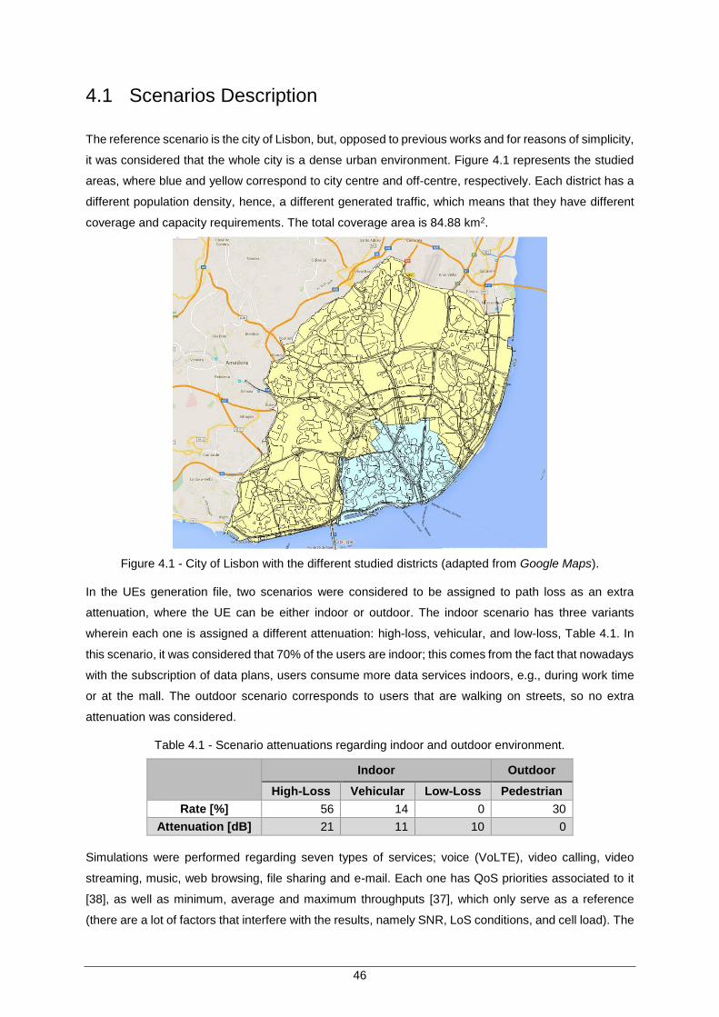
46
4.1 Scenarios Description
The reference scenario is the city of Lisbon, but, opposed to previous works and for reasons of simplicity,
it was considered that the whole city is a dense urban environment. Figure 4.1 represents the studied
areas, where blue and yellow correspond to city centre and off-centre, respectively. Each district has a
different population density, hence, a different generated traffic, which means that they have different
coverage and capacity requirements. The total coverage area is 84.88 km2.
Figure 4.1 - City of Lisbon with the different studied districts (adapted from Google Maps).
In the UEs generation file, two scenarios were considered to be assigned to path loss as an extra
attenuation, where the UE can be either indoor or outdoor. The indoor scenario has three variants
wherein each one is assigned a different attenuation: high-loss, vehicular, and low-loss, Table 4.1. In
this scenario, it was considered that 70% of the users are indoor; this comes from the fact that nowadays
with the subscription of data plans, users consume more data services indoors, e.g., during work time
or at the mall. The outdoor scenario corresponds to users that are walking on streets, so no extra
attenuation was considered.
Table 4.1 - Scenario attenuations regarding indoor and outdoor environment.
Indoor Outdoor
High-Loss Vehicular Low-Loss Pedestrian
Rate [%] 56 14 0 30
Attenuation [dB] 21 11 10 0
Simulations were performed regarding seven types of services; voice (VoLTE), video calling, video
streaming, music, web browsing, file sharing and e-mail. Each one has QoS priorities associated to it
[38], as well as minimum, average and maximum throughputs [37], which only serve as a reference
(there are a lot of factors that interfere with the results, namely SNR, LoS conditions, and cell load). The
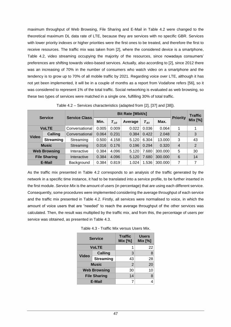
47
maximum throughput of Web Browsing, File Sharing and E-Mail in Table 4.2 were changed to the
theoretical maximum DL data rate of LTE, because they are services with no specific GBR. Services
with lower priority indexes or higher priorities were the first ones to be treated, and therefore the first to
receive resources. The traffic mix was taken from [2], where the considered device is a smartphone,
Table 4.2, video streaming occupying the majority of the resources, since nowadays consumers’
preferences are shifting towards video-based services. Actually, also according to [2], since 2012 there
was an increasing of 70% in the number of consumers who watch video on a smartphone and the
tendency is to grow up to 70% of all mobile traffic by 2021. Regarding voice over LTE, although it has
not yet been implemented, it will be in a couple of months as a report from Vodafone refers [56], so it
was considered to represent 1% of the total traffic. Social networking is evaluated as web browsing, so
these two types of services were matched in a single one, fulfilling 30% of total traffic.
Table 4.2 – Services characteristics (adapted from [2], [37] and [38]).
Service Service Class Bit Rate [Mbit/s]
Priority Traffic Mix [%] Min. 𝑻𝑳𝑶 Average 𝑻𝑯𝑰 Max.
VoLTE Conversational 0.005 0.009 0.022 0.036 0.064 1 1
Video Calling Conversational 0.064 0.231 0.384 0.422 2.048 2 3
Streaming Streaming 0.500 4.158 5.120 6.304 13.000 3 43
Music Streaming 0.016 0.176 0.196 0.294 0.320 4 2
Web Browsing Interactive 0.384 4.096 5.120 7.680 300.000 5 30
File Sharing Interactive 0.384 4.096 5.120 7.680 300.000 6 14
E-Mail Background 0.384 0.819 1.024 1.536 300.000 7 7
As the traffic mix presented in Table 4.2 corresponds to an analysis of the traffic generated by the
network in a specific time instance, it had to be translated into a service profile, to be further inserted in
the first module. Service Mix is the amount of users (in percentage) that are using each different service.
Consequently, some procedures were implemented considering the average throughput of each service
and the traffic mix presented in Table 4.2. Firstly, all services were normalised to voice, in which the
amount of voice users that are “needed” to reach the average throughput of the other services was
calculated. Then, the result was multiplied by the traffic mix, and from this, the percentage of users per
service was obtained, as presented in Table 4.3.
Table 4.3 - Traffic Mix versus Users Mix.
Service Traffic Mix [%]
Users Mix [%]
VoLTE 1 22
Video Calling 3 8
Streaming 43 28
Music 2 20
Web Browsing 30 10
File Sharing 14 8
E-Mail 7 4
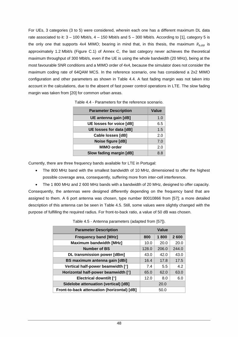
48
For UEs, 3 categories (3 to 5) were considered, wherein each one has a different maximum DL data
rate associated to it: 3 – 100 Mbit/s, 4 – 150 Mbit/s and 5 – 300 Mbit/s. According to [1], category 5 is
the only one that supports 4x4 MIMO; bearing in mind that, in this thesis, the maximum 𝑅𝑏,𝑅𝐵 is
approximately 1.2 Mbit/s (Figure C.1) of Annex C, the last category never achieves the theoretical
maximum throughput of 300 Mbit/s, even if the UE is using the whole bandwidth (20 MHz), being at the
most favourable SNR conditions and a MIMO order of 4x4, because the simulator does not consider the
maximum coding rate of 64QAM MCS. In the reference scenario, one has considered a 2x2 MIMO
configuration and other parameters as shown in Table 4.4. A fast fading margin was not taken into
account in the calculations, due to the absent of fast power control operations in LTE. The slow fading
margin was taken from [20] for common urban areas.
Table 4.4 - Parameters for the reference scenario.
Parameter Description Value
UE antenna gain [dB] 1.0
UE losses for voice [dB] 6.5
UE losses for data [dB] 1.5
Cable losses [dB] 2.0
Noise figure [dB] 7.0
MIMO order 2.0
Slow fading margin [dB] 8.8
Currently, there are three frequency bands available for LTE in Portugal:
The 800 MHz band with the smallest bandwidth of 10 MHz, dimensioned to offer the highest
possible coverage area, consequently, suffering more from inter-cell interference.
The 1 800 MHz and 2 600 MHz bands with a bandwidth of 20 MHz, designed to offer capacity.
Consequently, the antennas were designed differently depending on the frequency band that are
assigned to them. A 6 port antenna was chosen, type number 80010866 from [57]; a more detailed
description of this antenna can be seen in Table 4.5. Still, some values were slightly changed with the
purpose of fulfilling the required radius. For front-to-back ratio, a value of 50 dB was chosen.
Table 4.5 - Antenna parameters (adapted from [57]).
Parameter Description Value
Frequency band [MHz] 800 1 800 2 600
Maximum bandwidth [MHz] 10.0 20.0 20.0
Number of BS 128.0 206.0 244.0
DL transmission power [dBm] 43.0 42.0 43.0
BS maximum antenna gain [dBi] 16.4 17.8 17.5
Vertical half-power beamwidth [°] 7.4 5.5 4.2
Horizontal half-power beamwidth [°] 65.0 62.0 63.0
Electrical downtilt [°] 12.0 8.0 6.0
Sidelobe attenuation (vertical) [dB] 20.0
Front-to-back attenuation (horizontal) [dB] 50.0
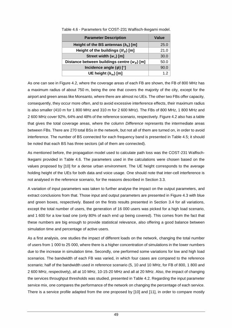
49
Table 4.6 - Parameters for COST-231 Walfisch-Ikegami model.
Parameter Description Value
Height of the BS antennas (𝒉𝒃) [m] 25.0
Height of the buildings (𝑯𝑩) [m] 21.0
Street width (𝒘𝒔) [m] 30.0
Distance between buildings centre (𝒘𝑩) [m] 50.0
Incidence angle (𝝓) [°] 90.0
UE height (𝒉𝒎) [m] 1.2
As one can see in Figure 4.2, where the coverage areas of each FB are shown, the FB of 800 MHz has
a maximum radius of about 750 m, being the one that covers the majority of the city, except for the
airport and green areas like Monsanto, where there are almost no UEs. The other two FBs offer capacity,
consequently, they occur more often, and to avoid excessive interference effects, their maximum radius
is also smaller (410 m for 1 800 MHz and 310 m for 2 600 MHz). The FBs of 800 MHz, 1 800 MHz and
2 600 MHz cover 92%, 64% and 48% of the reference scenario, respectively. Figure 4.2 also has a table
that gives the total coverage areas, where the column Difference represents the intermediate areas
between FBs. There are 270 total BSs in the network, but not all of them are turned on, in order to avoid
interference. The number of BS connected for each frequency band is presented in Table 4.5; it should
be noted that each BS has three sectors (all of them are connected).
As mentioned before, the propagation model used to calculate path loss was the COST-231 Walfisch-
Ikegami provided in Table 4.6. The parameters used in the calculations were chosen based on the
values proposed by [10] for a dense urban environment. The UE height corresponds to the average
holding height of the UEs for both data and voice usage. One should note that inter-cell interference is
not analysed in the reference scenario, for the reasons described in Section 3.3.
A variation of input parameters was taken to further analyse the impact on the output parameters, and
extract conclusions from that. Those input and output parameters are presented in Figure 4.3 with blue
and green boxes, respectively. Based on the firsts results presented in Section 3.4 for all variations,
except the total number of users, the generation of 16 000 users was picked for a high load scenario,
and 1 600 for a low load one (only 80% of each end up being covered). This comes from the fact that
these numbers are big enough to provide statistical relevance, also offering a good balance between
simulation time and percentage of active users.
As a first analysis, one studies the impact of different loads on the network, changing the total number
of users from 1 000 to 25 000, where there is a higher concentration of simulations in the lower numbers
due to the increase in simulation time. Secondly, one performed some variations for low and high load
scenarios. The bandwidth of each FB was varied, in which four cases are compared to the reference
scenario; half of the bandwidth used in reference scenario (5, 10 and 10 MHz, for FB of 800, 1 800 and
2 600 MHz, respectively), all at 10 MHz, 10-15-20 MHz and all at 20 MHz. Also, the impact of changing
the services throughput thresholds was studied, presented in Table 4.2. Regarding the input parameter
service mix, one compares the performance of the network on changing the percentage of each service.
There is a service profile adapted from the one proposed by [10] and [11], in order to compare mostly
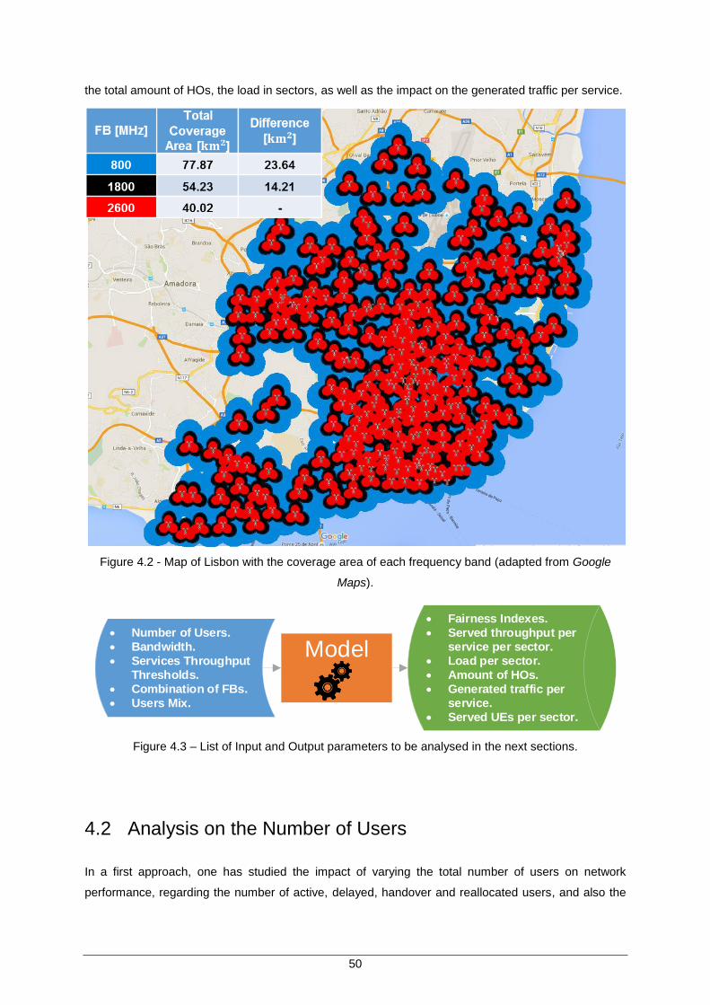
50
the total amount of HOs, the load in sectors, as well as the impact on the generated traffic per service.
Figure 4.2 - Map of Lisbon with the coverage area of each frequency band (adapted from Google
Maps).
Model Number of Users.
Bandwidth.
Services Throughput
Thresholds.
Combination of FBs.
Users Mix.
Fairness Indexes.
Served throughput per
service per sector.
Load per sector.
Amount of HOs.
Generated traffic per
service.
Served UEs per sector.
Figure 4.3 – List of Input and Output parameters to be analysed in the next sections.
4.2 Analysis on the Number of Users
In a first approach, one has studied the impact of varying the total number of users on network
performance, regarding the number of active, delayed, handover and reallocated users, and also the
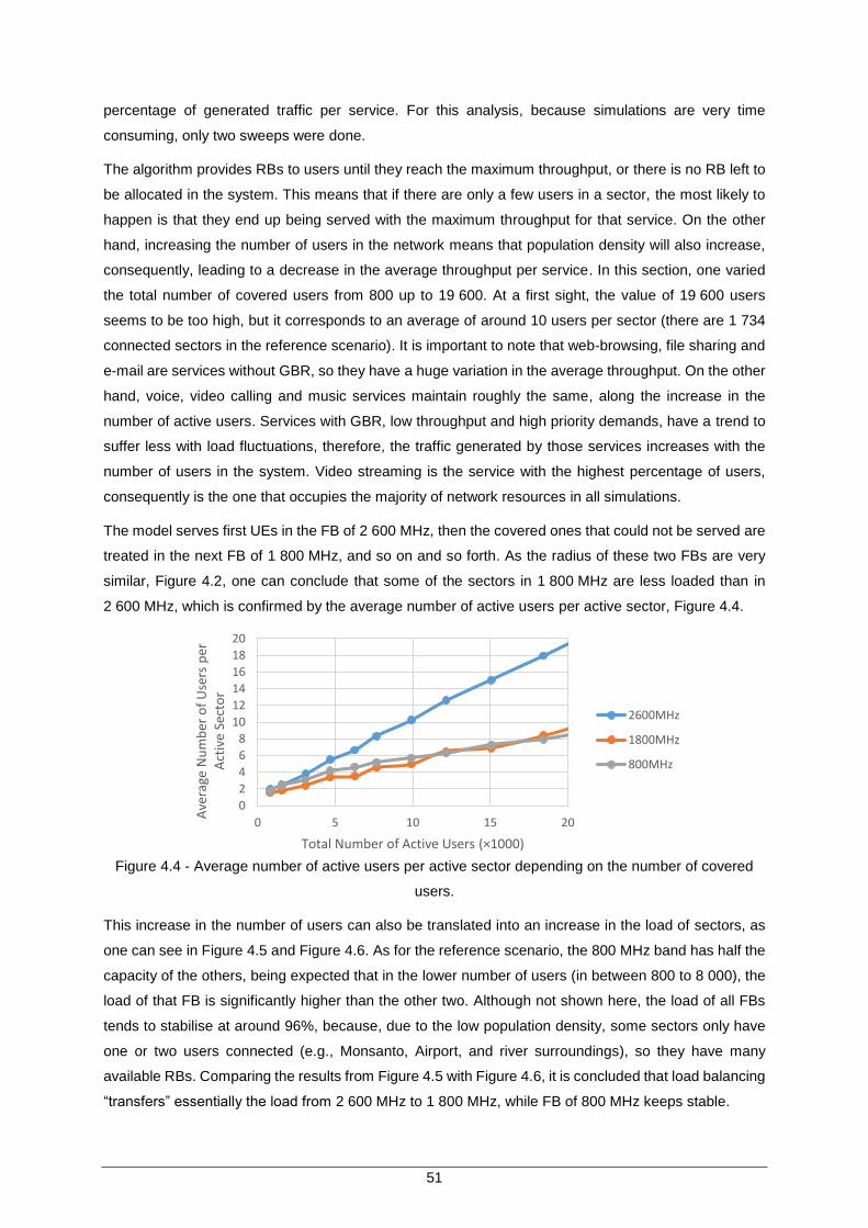
51
percentage of generated traffic per service. For this analysis, because simulations are very time
consuming, only two sweeps were done.
The algorithm provides RBs to users until they reach the maximum throughput, or there is no RB left to
be allocated in the system. This means that if there are only a few users in a sector, the most likely to
happen is that they end up being served with the maximum throughput for that service. On the other
hand, increasing the number of users in the network means that population density will also increase,
consequently, leading to a decrease in the average throughput per service. In this section, one varied
the total number of covered users from 800 up to 19 600. At a first sight, the value of 19 600 users
seems to be too high, but it corresponds to an average of around 10 users per sector (there are 1 734
connected sectors in the reference scenario). It is important to note that web-browsing, file sharing and
e-mail are services without GBR, so they have a huge variation in the average throughput. On the other
hand, voice, video calling and music services maintain roughly the same, along the increase in the
number of active users. Services with GBR, low throughput and high priority demands, have a trend to
suffer less with load fluctuations, therefore, the traffic generated by those services increases with the
number of users in the system. Video streaming is the service with the highest percentage of users,
consequently is the one that occupies the majority of network resources in all simulations.
The model serves first UEs in the FB of 2 600 MHz, then the covered ones that could not be served are
treated in the next FB of 1 800 MHz, and so on and so forth. As the radius of these two FBs are very
similar, Figure 4.2, one can conclude that some of the sectors in 1 800 MHz are less loaded than in
2 600 MHz, which is confirmed by the average number of active users per active sector, Figure 4.4.
Figure 4.4 - Average number of active users per active sector depending on the number of covered
users.
This increase in the number of users can also be translated into an increase in the load of sectors, as
one can see in Figure 4.5 and Figure 4.6. As for the reference scenario, the 800 MHz band has half the
capacity of the others, being expected that in the lower number of users (in between 800 to 8 000), the
load of that FB is significantly higher than the other two. Although not shown here, the load of all FBs
tends to stabilise at around 96%, because, due to the low population density, some sectors only have
one or two users connected (e.g., Monsanto, Airport, and river surroundings), so they have many
available RBs. Comparing the results from Figure 4.5 with Figure 4.6, it is concluded that load balancing
“transfers” essentially the load from 2 600 MHz to 1 800 MHz, while FB of 800 MHz keeps stable.
0
2
4
6
8
10
12
14
16
18
20
0 5 10 15 20
Ave
rage
Nu
mb
er o
f U
sers
per
A
ctiv
e Se
cto
r
Total Number of Active Users (×1000)
2600MHz
1800MHz
800MHz
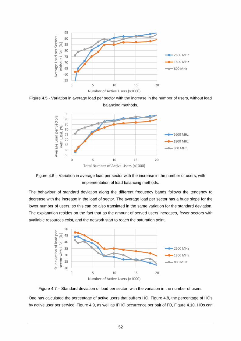
52
Figure 4.5 - Variation in average load per sector with the increase in the number of users, without load
balancing methods.
Figure 4.6 – Variation in average load per sector with the increase in the number of users, with
implementation of load balancing methods.
The behaviour of standard deviation along the different frequency bands follows the tendency to
decrease with the increase in the load of sector. The average load per sector has a huge slope for the
lower number of users, so this can be also translated in the same variation for the standard deviation.
The explanation resides on the fact that as the amount of served users increases, fewer sectors with
available resources exist, and the network start to reach the saturation point.
Figure 4.7 – Standard deviation of load per sector, with the variation in the number of users.
One has calculated the percentage of active users that suffers HO, Figure 4.8, the percentage of HOs
by active user per service, Figure 4.9, as well as IFHO occurrence per pair of FB, Figure 4.10. HOs can
55
60
65
70
75
80
85
90
95
0 5 10 15 20
Ave
rage
Lo
ad p
er S
ecto
rs
wit
ho
ut
L.B
al. [
%]
Number of Active Users (×1000)
2600 MHz
1800 MHz
800 MHz
55
60
65
70
75
80
85
90
95
0 5 10 15 20
Ave
rage
Lo
ad p
erSe
cto
rs
wit
h L
.Bal
. [%
]
Total Number of Active Users (×1000)
2600 MHz
1800 MHz
800 MHz
20
25
30
35
40
45
50
0 5 10 15 20
St. d
evia
tio
n o
f lo
ad p
erse
cto
r w
ith
L.B
al. [
%]
Number of Active Users (×1000)
2600 MHz
1800 MHz
800 MHz
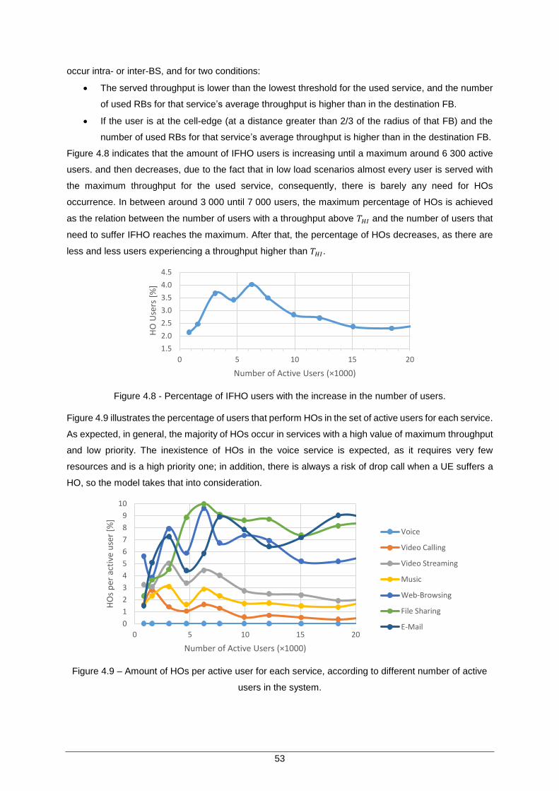
53
occur intra- or inter-BS, and for two conditions:
The served throughput is lower than the lowest threshold for the used service, and the number
of used RBs for that service’s average throughput is higher than in the destination FB.
If the user is at the cell-edge (at a distance greater than 2/3 of the radius of that FB) and the
number of used RBs for that service’s average throughput is higher than in the destination FB.
Figure 4.8 indicates that the amount of IFHO users is increasing until a maximum around 6 300 active
users. and then decreases, due to the fact that in low load scenarios almost every user is served with
the maximum throughput for the used service, consequently, there is barely any need for HOs
occurrence. In between around 3 000 until 7 000 users, the maximum percentage of HOs is achieved
as the relation between the number of users with a throughput above 𝑇𝐻𝐼 and the number of users that
need to suffer IFHO reaches the maximum. After that, the percentage of HOs decreases, as there are
less and less users experiencing a throughput higher than 𝑇𝐻𝐼.
Figure 4.8 - Percentage of IFHO users with the increase in the number of users.
Figure 4.9 illustrates the percentage of users that perform HOs in the set of active users for each service.
As expected, in general, the majority of HOs occur in services with a high value of maximum throughput
and low priority. The inexistence of HOs in the voice service is expected, as it requires very few
resources and is a high priority one; in addition, there is always a risk of drop call when a UE suffers a
HO, so the model takes that into consideration.
Figure 4.9 – Amount of HOs per active user for each service, according to different number of active
users in the system.
1.5
2.0
2.5
3.0
3.5
4.0
4.5
0 5 10 15 20
HO
Use
rs [
%]
Number of Active Users (×1000)
0
1
2
3
4
5
6
7
8
9
10
0 5 10 15 20
HO
s p
er a
ctiv
e u
ser
[%]
Number of Active Users (×1000)
Voice
Video Calling
Video Streaming
Music
Web-Browsing
File Sharing
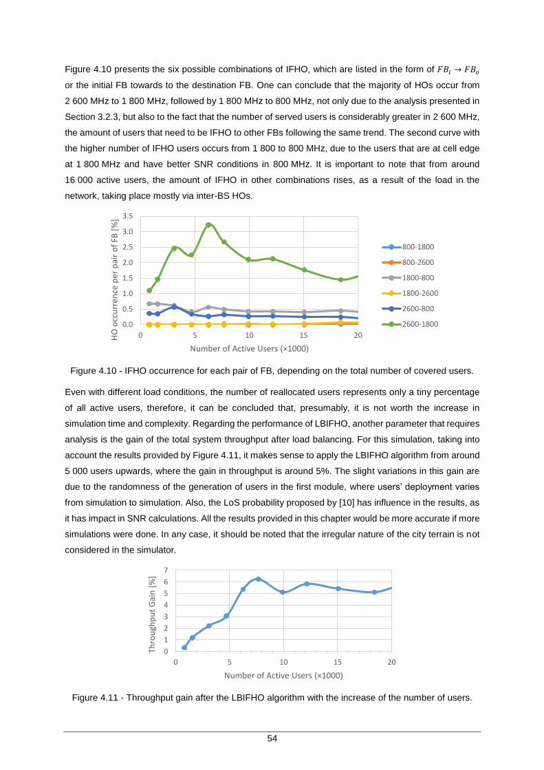
54
Figure 4.10 presents the six possible combinations of IFHO, which are listed in the form of 𝐹𝐵𝑖 → 𝐹𝐵𝑜
or the initial FB towards to the destination FB. One can conclude that the majority of HOs occur from
2 600 MHz to 1 800 MHz, followed by 1 800 MHz to 800 MHz, not only due to the analysis presented in
Section 3.2.3, but also to the fact that the number of served users is considerably greater in 2 600 MHz,
the amount of users that need to be IFHO to other FBs following the same trend. The second curve with
the higher number of IFHO users occurs from 1 800 to 800 MHz, due to the users that are at cell edge
at 1 800 MHz and have better SNR conditions in 800 MHz. It is important to note that from around
16 000 active users, the amount of IFHO in other combinations rises, as a result of the load in the
network, taking place mostly via inter-BS HOs.
Figure 4.10 - IFHO occurrence for each pair of FB, depending on the total number of covered users.
Even with different load conditions, the number of reallocated users represents only a tiny percentage
of all active users, therefore, it can be concluded that, presumably, it is not worth the increase in
simulation time and complexity. Regarding the performance of LBIFHO, another parameter that requires
analysis is the gain of the total system throughput after load balancing. For this simulation, taking into
account the results provided by Figure 4.11, it makes sense to apply the LBIFHO algorithm from around
5 000 users upwards, where the gain in throughput is around 5%. The slight variations in this gain are
due to the randomness of the generation of users in the first module, where users’ deployment varies
from simulation to simulation. Also, the LoS probability proposed by [10] has influence in the results, as
it has impact in SNR calculations. All the results provided in this chapter would be more accurate if more
simulations were done. In any case, it should be noted that the irregular nature of the city terrain is not
considered in the simulator.
Figure 4.11 - Throughput gain after the LBIFHO algorithm with the increase of the number of users.
0.0
0.5
1.0
1.5
2.0
2.5
3.0
3.5
0 5 10 15 20HO
occ
urr
ence
per
pai
r o
f FB
[%
]
Number of Active Users (×1000)
800-1800
800-2600
1800-800
1800-2600
2600-800
2600-1800
0
1
2
3
4
5
6
7
0 5 10 15 20
Thro
ugh
pu
t G
ain
[%
]
Number of Active Users (×1000)
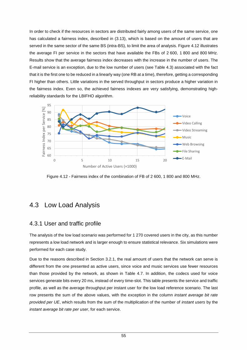
55
In order to check if the resources in sectors are distributed fairly among users of the same service, one
has calculated a fairness index, described in (3.13), which is based on the amount of users that are
served in the same sector of the same BS (intra-BS), to limit the area of analysis. Figure 4.12 illustrates
the average FI per service in the sectors that have available the FBs of 2 600, 1 800 and 800 MHz.
Results show that the average fairness index decreases with the increase in the number of users. The
E-mail service is an exception, due to the low number of users (see Table 4.3) associated with the fact
that it is the first one to be reduced in a linearly way (one RB at a time), therefore, getting a corresponding
FI higher than others. Little variations in the served throughput in sectors produce a higher variation in
the fairness index. Even so, the achieved fairness indexes are very satisfying, demonstrating high-
reliability standards for the LBIFHO algorithm.
Figure 4.12 - Fairness index of the combination of FB of 2 600, 1 800 and 800 MHz.
4.3 Low Load Analysis
4.3.1 User and traffic profile
The analysis of the low load scenario was performed for 1 270 covered users in the city, as this number
represents a low load network and is larger enough to ensure statistical relevance. Six simulations were
performed for each case study.
Due to the reasons described in Section 3.2.1, the real amount of users that the network can serve is
different from the one presented as active users, since voice and music services use fewer resources
than those provided by the network, as shown in Table 4.7. In addition, the codecs used for voice
services generate bits every 20 ms, instead of every time-slot. This table presents the service and traffic
profile, as well as the average throughput per instant user for the low load reference scenario. The last
row presents the sum of the above values, with the exception in the column instant average bit rate
provided per UE, which results from the sum of the multiplication of the number of instant users by the
instant average bit rate per user, for each service.
60
65
70
75
80
85
90
95
0 5 10 15 20
Fair
nes
s In
dex
per
Ser
vice
[%
]
Number of Active Users (×1000)
Voice
Video Calling
Video Streaming
Music
Web Browsing
File Sharing
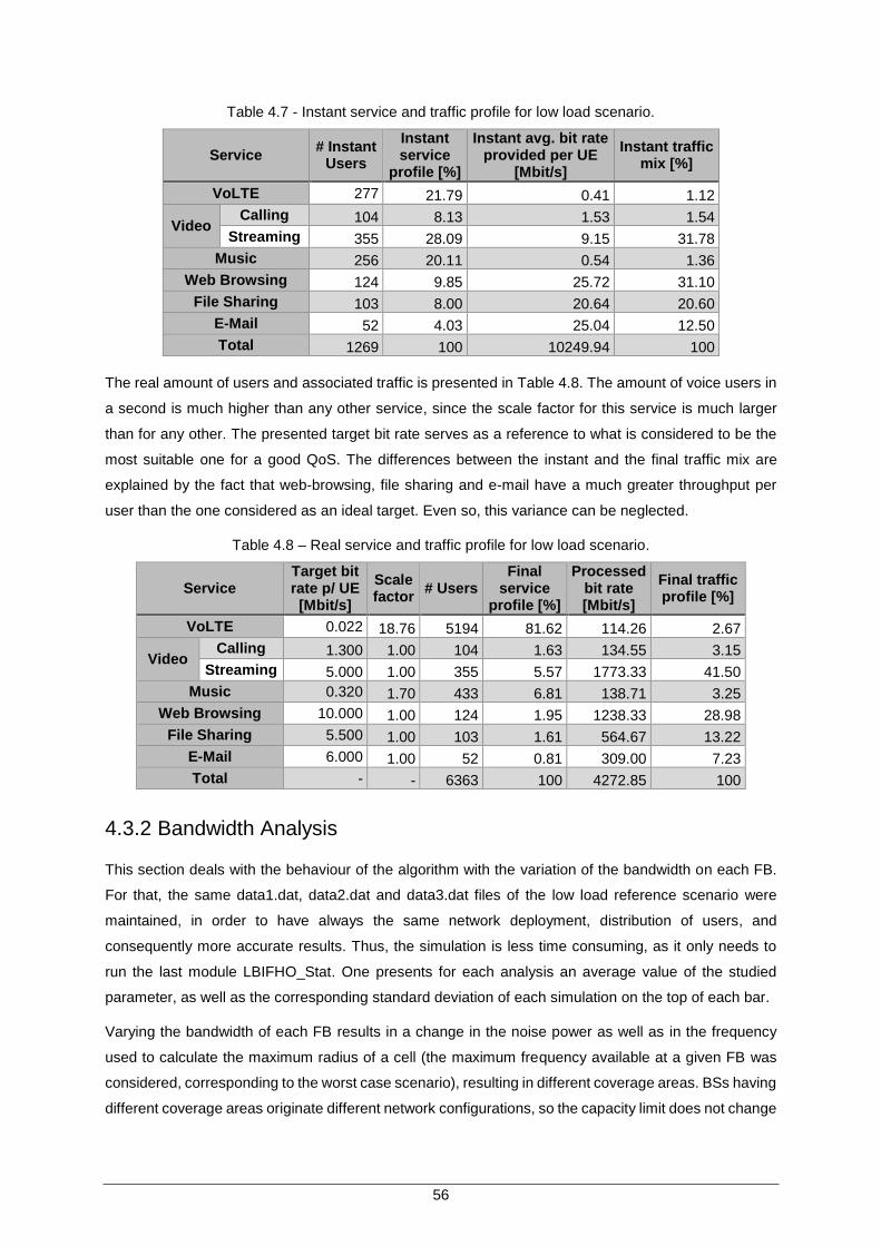
56
Table 4.7 - Instant service and traffic profile for low load scenario.
Service # Instant
Users
Instant service
profile [%]
Instant avg. bit rate provided per UE
[Mbit/s]
Instant traffic mix [%]
VoLTE 277 21.79 0.41 1.12
Video Calling 104 8.13 1.53 1.54
Streaming 355 28.09 9.15 31.78
Music 256 20.11 0.54 1.36
Web Browsing 124 9.85 25.72 31.10
File Sharing 103 8.00 20.64 20.60
E-Mail 52 4.03 25.04 12.50
Total 1269 100 10249.94 100
The real amount of users and associated traffic is presented in Table 4.8. The amount of voice users in
a second is much higher than any other service, since the scale factor for this service is much larger
than for any other. The presented target bit rate serves as a reference to what is considered to be the
most suitable one for a good QoS. The differences between the instant and the final traffic mix are
explained by the fact that web-browsing, file sharing and e-mail have a much greater throughput per
user than the one considered as an ideal target. Even so, this variance can be neglected.
Table 4.8 – Real service and traffic profile for low load scenario.
Service Target bit rate p/ UE [Mbit/s]
Scale factor
# Users Final
service profile [%]
Processed bit rate [Mbit/s]
Final traffic profile [%]
VoLTE 0.022 18.76 5194 81.62 114.26 2.67
Video Calling 1.300 1.00 104 1.63 134.55 3.15
Streaming 5.000 1.00 355 5.57 1773.33 41.50
Music 0.320 1.70 433 6.81 138.71 3.25
Web Browsing 10.000 1.00 124 1.95 1238.33 28.98
File Sharing 5.500 1.00 103 1.61 564.67 13.22
E-Mail 6.000 1.00 52 0.81 309.00 7.23
Total - - 6363 100 4272.85 100
4.3.2 Bandwidth Analysis
This section deals with the behaviour of the algorithm with the variation of the bandwidth on each FB.
For that, the same data1.dat, data2.dat and data3.dat files of the low load reference scenario were
maintained, in order to have always the same network deployment, distribution of users, and
consequently more accurate results. Thus, the simulation is less time consuming, as it only needs to
run the last module LBIFHO_Stat. One presents for each analysis an average value of the studied
parameter, as well as the corresponding standard deviation of each simulation on the top of each bar.
Varying the bandwidth of each FB results in a change in the noise power as well as in the frequency
used to calculate the maximum radius of a cell (the maximum frequency available at a given FB was
considered, corresponding to the worst case scenario), resulting in different coverage areas. BSs having
different coverage areas originate different network configurations, so the capacity limit does not change
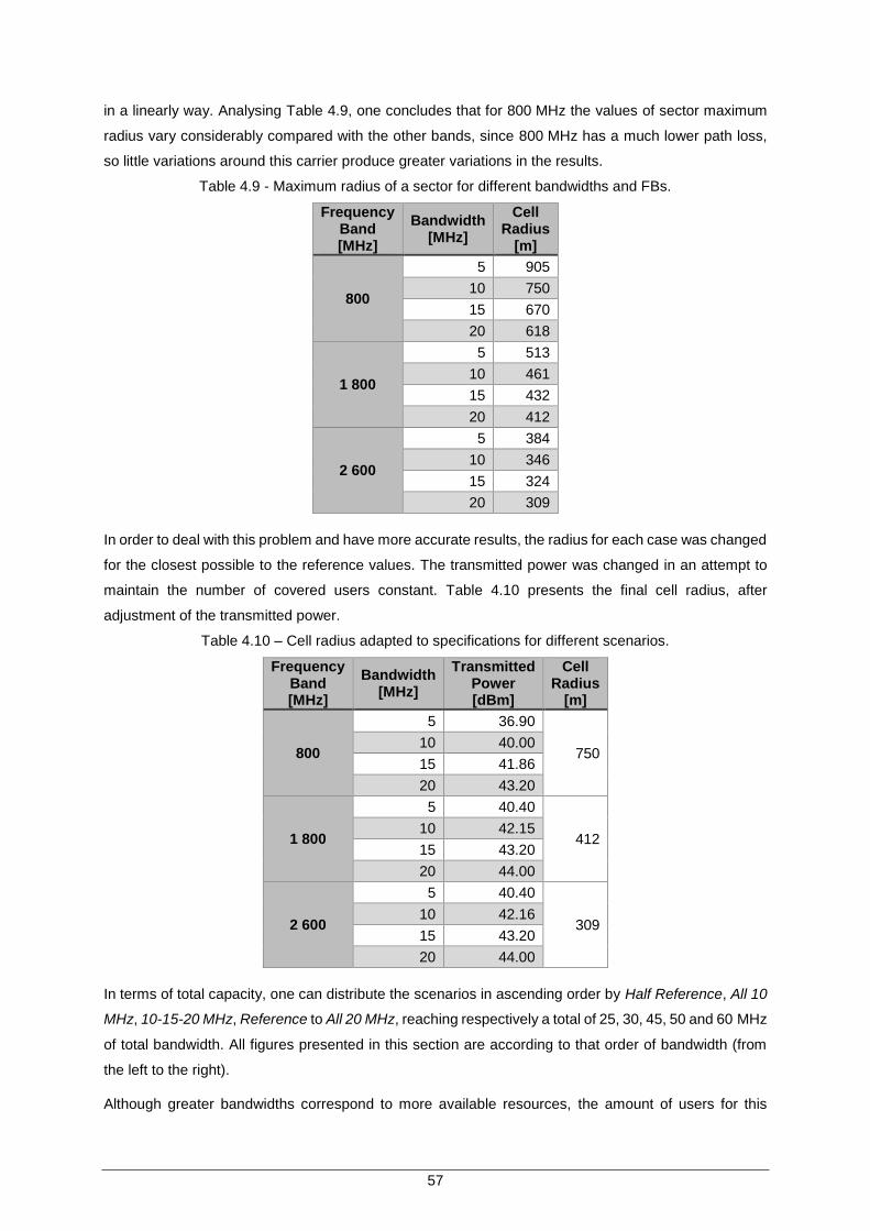
57
in a linearly way. Analysing Table 4.9, one concludes that for 800 MHz the values of sector maximum
radius vary considerably compared with the other bands, since 800 MHz has a much lower path loss,
so little variations around this carrier produce greater variations in the results.
Table 4.9 - Maximum radius of a sector for different bandwidths and FBs.
Frequency Band [MHz]
Bandwidth [MHz]
Cell Radius
[m]
800
5 905
10 750
15 670
20 618
1 800
5 513
10 461
15 432
20 412
2 600
5 384
10 346
15 324
20 309
In order to deal with this problem and have more accurate results, the radius for each case was changed
for the closest possible to the reference values. The transmitted power was changed in an attempt to
maintain the number of covered users constant. Table 4.10 presents the final cell radius, after
adjustment of the transmitted power.
Table 4.10 – Cell radius adapted to specifications for different scenarios.
Frequency Band [MHz]
Bandwidth [MHz]
Transmitted Power [dBm]
Cell Radius
[m]
800
5 36.90
750 10 40.00
15 41.86
20 43.20
1 800
5 40.40
412 10 42.15
15 43.20
20 44.00
2 600
5 40.40
309 10 42.16
15 43.20
20 44.00
In terms of total capacity, one can distribute the scenarios in ascending order by Half Reference, All 10
MHz, 10-15-20 MHz, Reference to All 20 MHz, reaching respectively a total of 25, 30, 45, 50 and 60 MHz
of total bandwidth. All figures presented in this section are according to that order of bandwidth (from
the left to the right).
Although greater bandwidths correspond to more available resources, the amount of users for this
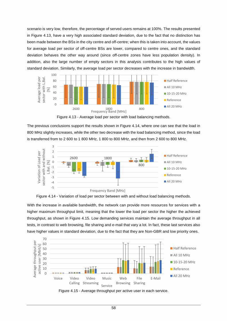
58
scenario is very low, therefore, the percentage of served users remains at 100%. The results presented
in Figure 4.13, have a very high associated standard deviation, due to the fact that no distinction has
been made between the BSs in the city centre and off-centre; when this is taken into account, the values
for average load per sector of off-centre BSs are lower, compared to centre ones, and the standard
deviation behaves the other way around (since off-centre zones have less population density). In
addition, also the large number of empty sectors in this analysis contributes to the high values of
standard deviation. Similarly, the average load per sector decreases with the increase in bandwidth.
Figure 4.13 - Average load per sector with load balancing methods.
The previous conclusions support the results shown in Figure 4.14, where one can see that the load in
800 MHz slightly increases, while the other two decrease with the load balancing method, since the load
is transferred from to 2 600 to 1 800 MHz, 1 800 to 800 MHz, and then from 2 600 to 800 MHz.
Figure 4.14 - Variation of load per sector between with and without load balancing methods.
With the increase in available bandwidth, the network can provide more resources for services with a
higher maximum throughput limit, meaning that the lower the load per sector the higher the achieved
throughput, as shown in Figure 4.15. Low demanding services maintain the average throughput in all
tests, in contrast to web browsing, file sharing and e-mail that vary a lot. In fact, these last services also
have higher values in standard deviation, due to the fact that they are Non-GBR and low priority ones.
Figure 4.15 - Average throughput per active user in each service.
0
20
40
60
80
100
2600 1800 800
Ave
rage
load
per
se
cto
r w
ith
L.B
al.
[%]
Frequency Band [MHz]
Half Reference
All 10 MHz
10-15-20 MHz
Reference
All 20 MHz
-5
-4
-3
-2
-1
0
1
2
3
Var
iati
on
of
Load
per
se
cto
r w
ith
an
d w
ith
ou
t L.
Bal
. [%
]
Frequency Band [MHz]
Half Reference
All 10 MHz
10-15-20 MHz
Reference
All 20 MHz
800
18002600
0
10
20
30
40
50
60
70
Voice VideoCalling
VideoStreaming
Music WebBrowsing
FileSharing
Ave
rage
th
rou
ghp
ut
per
ac
tive
use
r [M
bit
/s]
Service
Half Reference
All 10 MHz
10-15-20 MHz
Reference
All 20 MHz
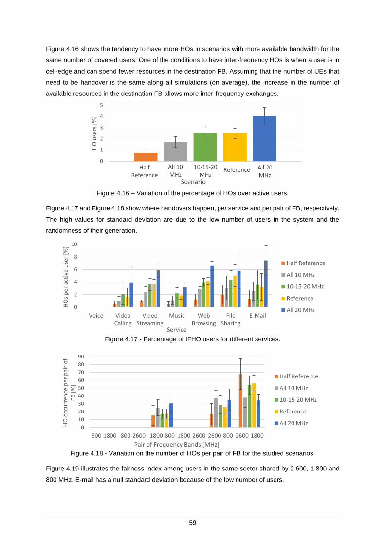
59
Figure 4.16 shows the tendency to have more HOs in scenarios with more available bandwidth for the
same number of covered users. One of the conditions to have inter-frequency HOs is when a user is in
cell-edge and can spend fewer resources in the destination FB. Assuming that the number of UEs that
need to be handover is the same along all simulations (on average), the increase in the number of
available resources in the destination FB allows more inter-frequency exchanges.
Figure 4.16 – Variation of the percentage of HOs over active users.
Figure 4.17 and Figure 4.18 show where handovers happen, per service and per pair of FB, respectively.
The high values for standard deviation are due to the low number of users in the system and the
randomness of their generation.
Figure 4.17 - Percentage of IFHO users for different services.
Figure 4.18 - Variation on the number of HOs per pair of FB for the studied scenarios.
Figure 4.19 illustrates the fairness index among users in the same sector shared by 2 600, 1 800 and
800 MHz. E-mail has a null standard deviation because of the low number of users.
0
1
2
3
4
5
HO
use
rs [
%]
All 20 MHz
Half Reference
Scenario
ReferenceAll 10 MHz
10-15-20
MHz
0
2
4
6
8
10
Voice VideoCalling
VideoStreaming
Music WebBrowsing
FileSharing
HO
s p
er a
ctiv
e u
ser
[%]
Service
Half Reference
All 10 MHz
10-15-20 MHz
Reference
All 20 MHz
0
10
20
30
40
50
60
70
80
90
800-1800 800-2600 1800-800 1800-2600 2600-800 2600-1800
HO
occ
urr
ence
per
pai
r o
f FB
[%
]
Pair of Frequency Bands [MHz]
Half Reference
All 10 MHz
10-15-20 MHz
Reference
All 20 MHz
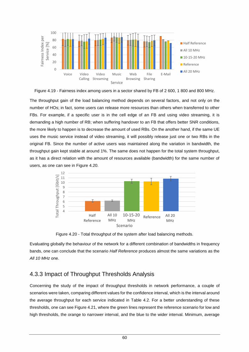
60
Figure 4.19 - Fairness index among users in a sector shared by FB of 2 600, 1 800 and 800 MHz.
The throughput gain of the load balancing method depends on several factors, and not only on the
number of HOs; in fact, some users can release more resources than others when transferred to other
FBs. For example, if a specific user is in the cell edge of an FB and using video streaming, it is
demanding a high number of RB; when suffering handover to an FB that offers better SNR conditions,
the more likely to happen is to decrease the amount of used RBs. On the another hand, if the same UE
uses the music service instead of video streaming, it will possibly release just one or two RBs in the
original FB. Since the number of active users was maintained along the variation in bandwidth, the
throughput gain kept stable at around 1%. The same does not happen for the total system throughput,
as it has a direct relation with the amount of resources available (bandwidth) for the same number of
users, as one can see in Figure 4.20.
Figure 4.20 - Total throughput of the system after load balancing methods.
Evaluating globally the behaviour of the network for a different combination of bandwidths in frequency
bands, one can conclude that the scenario Half Reference produces almost the same variations as the
All 10 MHz one.
4.3.3 Impact of Throughput Thresholds Analysis
Concerning the study of the impact of throughput thresholds in network performance, a couple of
scenarios were taken, comparing different values for the confidence interval, which is the interval around
the average throughput for each service indicated in Table 4.2. For a better understanding of these
thresholds, one can see Figure 4.21, where the green lines represent the reference scenario for low and
high thresholds, the orange to narrower interval, and the blue to the wider interval. Minimum, average
0
20
40
60
80
100
Voice VideoCalling
VideoStreaming
Music WebBrowsing
FileSharing
Fair
nes
s In
dex
per
Se
rvic
e [%
]
Service
Half Reference
All 10 MHz
10-15-20 MHz
Reference
All 20 MHz
4
5
6
7
8
9
10
11
12
Tota
l Th
rou
ghp
ut
[Gb
it/s
]
All 20 MHz
Half Reference
Scenario
ReferenceAll 10 MHz
10-15-20 MHz
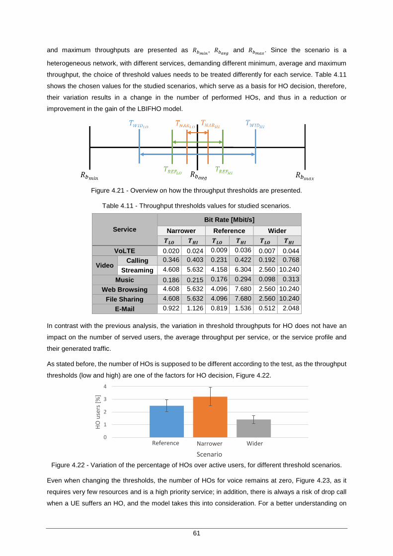
61
and maximum throughputs are presented as 𝑅𝑏𝑚𝑖𝑛, 𝑅𝑏𝑎𝑣𝑔
and 𝑅𝑏𝑚𝑎𝑥. Since the scenario is a
heterogeneous network, with different services, demanding different minimum, average and maximum
throughput, the choice of threshold values needs to be treated differently for each service. Table 4.11
shows the chosen values for the studied scenarios, which serve as a basis for HO decision, therefore,
their variation results in a change in the number of performed HOs, and thus in a reduction or
improvement in the gain of the LBIFHO model.
Figure 4.21 - Overview on how the throughput thresholds are presented.
Table 4.11 - Throughput thresholds values for studied scenarios.
Service
Bit Rate [Mbit/s]
Narrower Reference Wider
𝑻𝑳𝑶 𝑻𝑯𝑰 𝑻𝑳𝑶 𝑻𝑯𝑰 𝑻𝑳𝑶 𝑻𝑯𝑰
VoLTE 0.020 0.024 0.009 0.036 0.007 0.044
Video Calling 0.346 0.403 0.231 0.422 0.192 0.768
Streaming 4.608 5.632 4.158 6.304 2.560 10.240
Music 0.186 0.215 0.176 0.294 0.098 0.313
Web Browsing 4.608 5.632 4.096 7.680 2.560 10.240
File Sharing 4.608 5.632 4.096 7.680 2.560 10.240
E-Mail 0.922 1.126 0.819 1.536 0.512 2.048
In contrast with the previous analysis, the variation in threshold throughputs for HO does not have an
impact on the number of served users, the average throughput per service, or the service profile and
their generated traffic.
As stated before, the number of HOs is supposed to be different according to the test, as the throughput
thresholds (low and high) are one of the factors for HO decision, Figure 4.22.
Figure 4.22 - Variation of the percentage of HOs over active users, for different threshold scenarios.
Even when changing the thresholds, the number of HOs for voice remains at zero, Figure 4.23, as it
requires very few resources and is a high priority service; in addition, there is always a risk of drop call
when a UE suffers an HO, and the model takes this into consideration. For a better understanding on
0
1
2
3
4
HO
use
rs [
%]
WiderNarrowerReference
Scenario
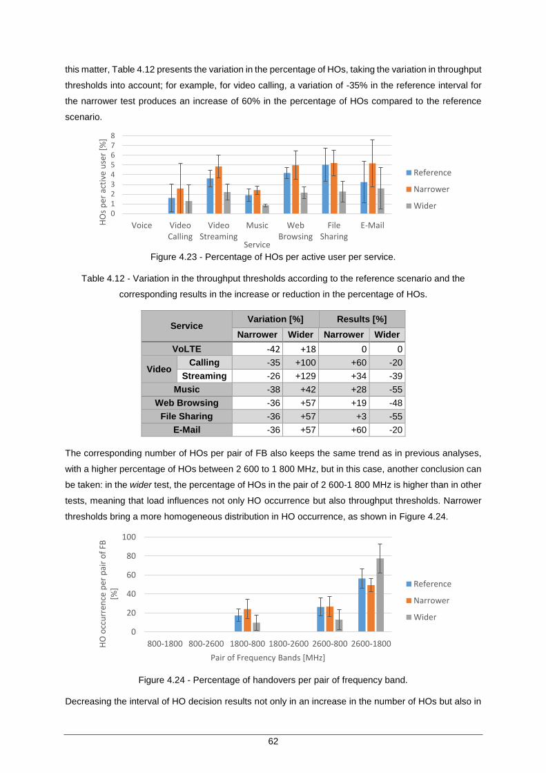
62
this matter, Table 4.12 presents the variation in the percentage of HOs, taking the variation in throughput
thresholds into account; for example, for video calling, a variation of -35% in the reference interval for
the narrower test produces an increase of 60% in the percentage of HOs compared to the reference
scenario.
Figure 4.23 - Percentage of HOs per active user per service.
Table 4.12 - Variation in the throughput thresholds according to the reference scenario and the
corresponding results in the increase or reduction in the percentage of HOs.
Service Variation [%] Results [%]
Narrower Wider Narrower Wider
VoLTE -42 +18 0 0
Video Calling -35 +100 +60 -20
Streaming -26 +129 +34 -39
Music -38 +42 +28 -55
Web Browsing -36 +57 +19 -48
File Sharing -36 +57 +3 -55
E-Mail -36 +57 +60 -20
The corresponding number of HOs per pair of FB also keeps the same trend as in previous analyses,
with a higher percentage of HOs between 2 600 to 1 800 MHz, but in this case, another conclusion can
be taken: in the wider test, the percentage of HOs in the pair of 2 600-1 800 MHz is higher than in other
tests, meaning that load influences not only HO occurrence but also throughput thresholds. Narrower
thresholds bring a more homogeneous distribution in HO occurrence, as shown in Figure 4.24.
Figure 4.24 - Percentage of handovers per pair of frequency band.
Decreasing the interval of HO decision results not only in an increase in the number of HOs but also in
012345678
Voice VideoCalling
VideoStreaming
Music WebBrowsing
FileSharing
E-MailHO
s p
er a
ctiv
e u
ser
[%]
Service
Reference
Narrower
Wider
0
20
40
60
80
100
800-1800 800-2600 1800-800 1800-2600 2600-800 2600-1800HO
occ
urr
ence
per
pai
r o
f FB
[%
]
Pair of Frequency Bands [MHz]
Reference
Narrower
Wider
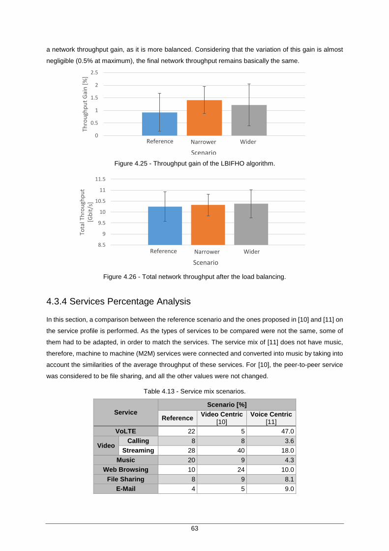
63
a network throughput gain, as it is more balanced. Considering that the variation of this gain is almost
negligible (0.5% at maximum), the final network throughput remains basically the same.
Figure 4.25 - Throughput gain of the LBIFHO algorithm.
Figure 4.26 - Total network throughput after the load balancing.
4.3.4 Services Percentage Analysis
In this section, a comparison between the reference scenario and the ones proposed in [10] and [11] on
the service profile is performed. As the types of services to be compared were not the same, some of
them had to be adapted, in order to match the services. The service mix of [11] does not have music,
therefore, machine to machine (M2M) services were connected and converted into music by taking into
account the similarities of the average throughput of these services. For [10], the peer-to-peer service
was considered to be file sharing, and all the other values were not changed.
Table 4.13 - Service mix scenarios.
Service
Scenario [%]
Reference Video Centric
[10] Voice Centric
[11]
VoLTE 22 5 47.0
Video Calling 8 8 3.6
Streaming 28 40 18.0
Music 20 9 4.3
Web Browsing 10 24 10.0
File Sharing 8 9 8.1
E-Mail 4 5 9.0
0
0.5
1
1.5
2
2.5
Thro
ugh
pu
t G
ain
[%
]
WiderNarrowerReference
Scenario
8.5
9
9.5
10
10.5
11
11.5
Tota
l Th
rou
ghp
ut
[Gb
it/s
]
WiderNarrowerReference
Scenario
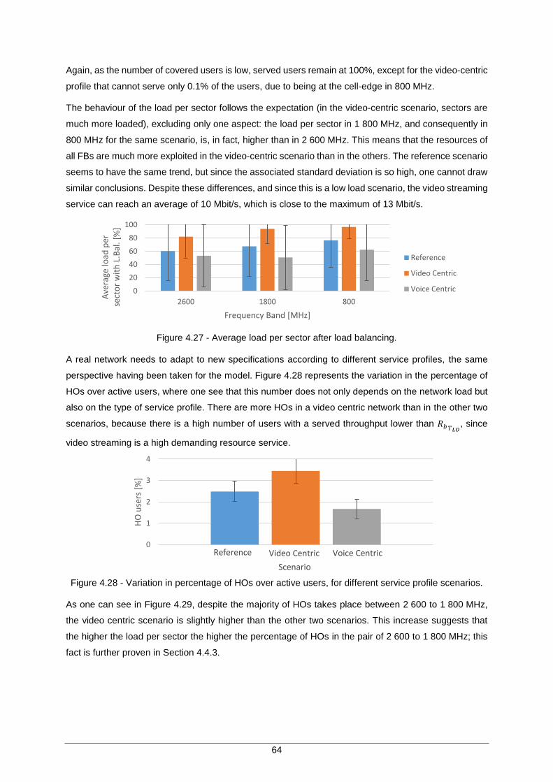
64
Again, as the number of covered users is low, served users remain at 100%, except for the video-centric
profile that cannot serve only 0.1% of the users, due to being at the cell-edge in 800 MHz.
The behaviour of the load per sector follows the expectation (in the video-centric scenario, sectors are
much more loaded), excluding only one aspect: the load per sector in 1 800 MHz, and consequently in
800 MHz for the same scenario, is, in fact, higher than in 2 600 MHz. This means that the resources of
all FBs are much more exploited in the video-centric scenario than in the others. The reference scenario
seems to have the same trend, but since the associated standard deviation is so high, one cannot draw
similar conclusions. Despite these differences, and since this is a low load scenario, the video streaming
service can reach an average of 10 Mbit/s, which is close to the maximum of 13 Mbit/s.
Figure 4.27 - Average load per sector after load balancing.
A real network needs to adapt to new specifications according to different service profiles, the same
perspective having been taken for the model. Figure 4.28 represents the variation in the percentage of
HOs over active users, where one see that this number does not only depends on the network load but
also on the type of service profile. There are more HOs in a video centric network than in the other two
scenarios, because there is a high number of users with a served throughput lower than 𝑅𝑏 𝑇𝐿𝑂, since
video streaming is a high demanding resource service.
Figure 4.28 - Variation in percentage of HOs over active users, for different service profile scenarios.
As one can see in Figure 4.29, despite the majority of HOs takes place between 2 600 to 1 800 MHz,
the video centric scenario is slightly higher than the other two scenarios. This increase suggests that
the higher the load per sector the higher the percentage of HOs in the pair of 2 600 to 1 800 MHz; this
fact is further proven in Section 4.4.3.
0
20
40
60
80
100
2600 1800 800
Ave
rage
load
per
se
cto
r w
ith
L.B
al. [
%]
Frequency Band [MHz]
Reference
Video Centric
Voice Centric
0
1
2
3
4
HO
use
rs [
%]
Voice CentricVideo CentricReference
Scenario
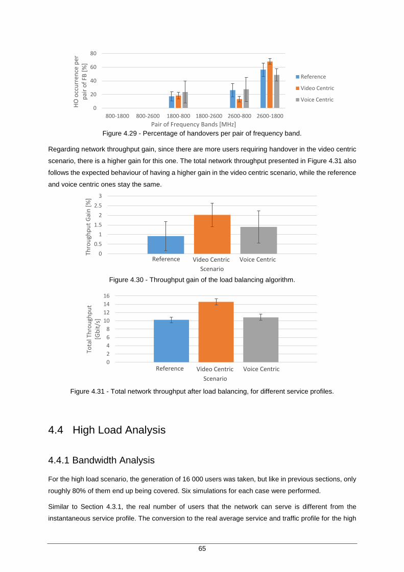
65
Figure 4.29 - Percentage of handovers per pair of frequency band.
Regarding network throughput gain, since there are more users requiring handover in the video centric
scenario, there is a higher gain for this one. The total network throughput presented in Figure 4.31 also
follows the expected behaviour of having a higher gain in the video centric scenario, while the reference
and voice centric ones stay the same.
Figure 4.30 - Throughput gain of the load balancing algorithm.
Figure 4.31 - Total network throughput after load balancing, for different service profiles.
4.4 High Load Analysis
4.4.1 Bandwidth Analysis
For the high load scenario, the generation of 16 000 users was taken, but like in previous sections, only
roughly 80% of them end up being covered. Six simulations for each case were performed.
Similar to Section 4.3.1, the real number of users that the network can serve is different from the
instantaneous service profile. The conversion to the real average service and traffic profile for the high
0
20
40
60
80
800-1800 800-2600 1800-800 1800-2600 2600-800 2600-1800
HO
occ
urr
ence
per
p
air
of
FB [
%]
Pair of Frequency Bands [MHz]
Reference
Video Centric
Voice Centric
0
0.5
1
1.5
2
2.5
3
Thro
ugh
pu
t G
ain
[%
]
Voice CentricVideo CentricReference
Scenario
0
2
4
6
8
10
12
14
16
Tota
l Th
rou
ghp
ut
[Gb
it/s
]
Voice CentricVideo CentricReference
Scenario
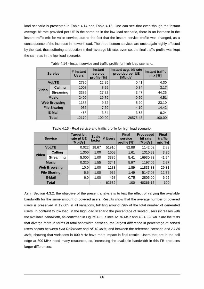
66
load scenario is presented in Table 4.14 and Table 4.15. One can see that even though the instant
average bit rate provided per UE is the same as in the low load scenario, there is an increase in the
instant traffic mix for voice service, due to the fact that the instant service profile was changed, as a
consequence of the increase in network load. The three bottom services are once again highly affected
by the load, thus suffering a reduction in their average bit rate, even so, the final traffic profile was kept
the same as in the low load scenario.
Table 4.14 - Instant service and traffic profile for high load scenario.
Service # Instant
Users
Instant service
profile [%]
Instant avg. bit rate provided per UE
[Mbit/s]
Instant traffic mix [%]
VoLTE 2780 22.85 0.41 4.30
Video Calling 1008 8.29 0.84 3.17
Streaming 3386 27.82 3.47 44.26
Music 2409 19.79 0.50 4.51
Web Browsing 1183 9.72 5.20 23.10
File Sharing 936 7.69 4.10 14.42
E-Mail 468 3.84 3.53 6.24
Total 12170 100.00 26575.48 100.00
Table 4.15 - Real service and traffic profile for high load scenario.
Service Target bit rate p/ UE [Mbit/s]
Scale factor
# Users Final
service profile [%]
Processed bit rate [Mbit/s]
Final traffic
mix [%]
VoLTE 0.022 18.67 51910 82.88 1142.02 2.83
Video Calling 1.300 1.00 1008 1.61 1310.83 3.25
Streaming 5.000 1.00 3386 5.41 16930.83 41.94
Music 0.320 1.55 3741 5.97 1197.06 2.97
Web Browsing 10.0 1.00 1183 1.89 11833.33 29.31
File Sharing 5.5 1.00 936 1.49 5147.08 12.75
E-Mail 6.0 1.00 468 0.75 2805.00 6.95
Total - - 62632 100 40366.16 100
As in Section 4.3.2, the objective of the present analysis is to test the effect of varying the available
bandwidth for the same amount of covered users. Results show that the average number of covered
users is preserved at 12 605 in all variations, fulfilling around 79% of the total number of generated
users. In contrast to low load, in the high load scenario the percentage of served users increases with
the available bandwidth, as confirmed in Figure 4.32. Since All 10 MHz and 10-15-20 MHz are the tests
that diverge more in terms of total bandwidth between, the largest difference in percentage of served
users occurs between Half Reference and All 10 MHz, and between the reference scenario and All 20
MHz, showing that variations in 800 MHz have more impact in final results. Users that are in the cell
edge at 800 MHz need many resources, so, increasing the available bandwidth in this FB produces
larger differences.
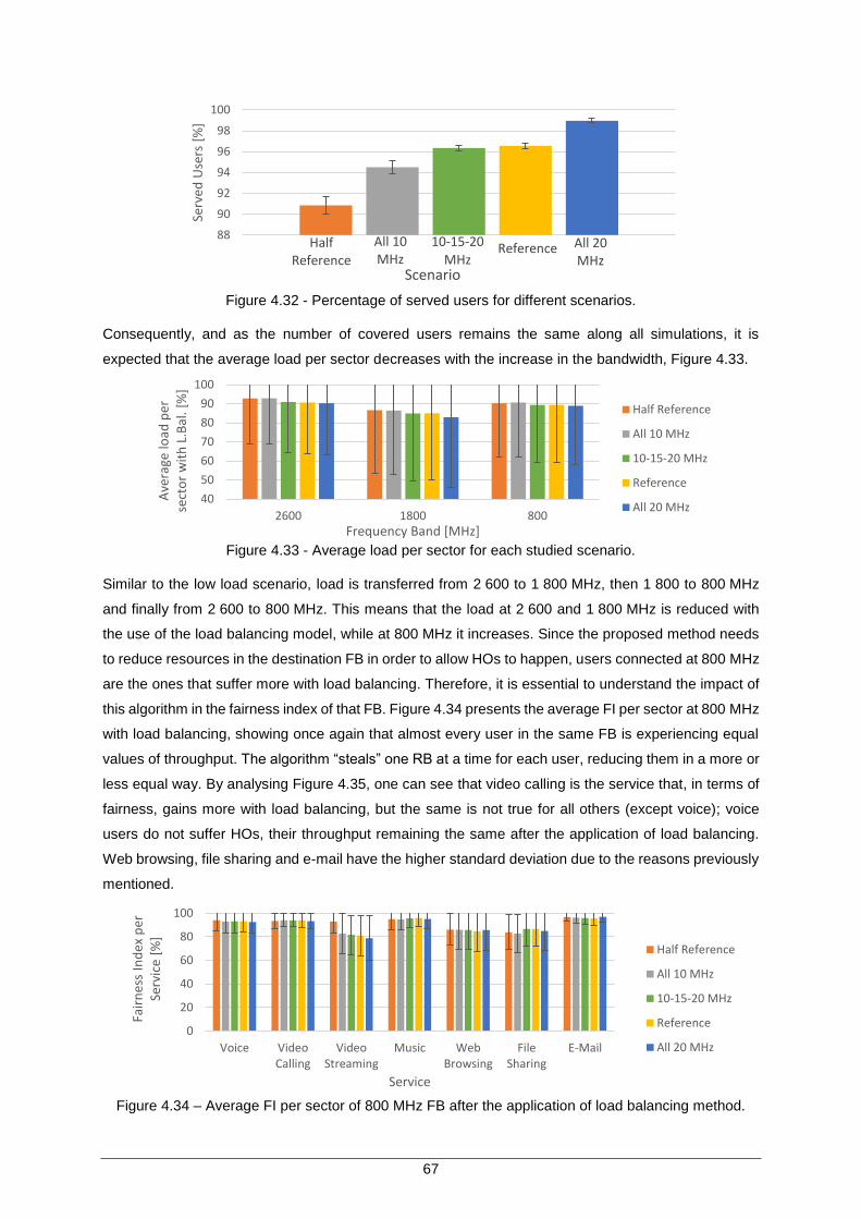
67
Figure 4.32 - Percentage of served users for different scenarios.
Consequently, and as the number of covered users remains the same along all simulations, it is
expected that the average load per sector decreases with the increase in the bandwidth, Figure 4.33.
Figure 4.33 - Average load per sector for each studied scenario.
Similar to the low load scenario, load is transferred from 2 600 to 1 800 MHz, then 1 800 to 800 MHz
and finally from 2 600 to 800 MHz. This means that the load at 2 600 and 1 800 MHz is reduced with
the use of the load balancing model, while at 800 MHz it increases. Since the proposed method needs
to reduce resources in the destination FB in order to allow HOs to happen, users connected at 800 MHz
are the ones that suffer more with load balancing. Therefore, it is essential to understand the impact of
this algorithm in the fairness index of that FB. Figure 4.34 presents the average FI per sector at 800 MHz
with load balancing, showing once again that almost every user in the same FB is experiencing equal
values of throughput. The algorithm “steals” one RB at a time for each user, reducing them in a more or
less equal way. By analysing Figure 4.35, one can see that video calling is the service that, in terms of
fairness, gains more with load balancing, but the same is not true for all others (except voice); voice
users do not suffer HOs, their throughput remaining the same after the application of load balancing.
Web browsing, file sharing and e-mail have the higher standard deviation due to the reasons previously
mentioned.
Figure 4.34 – Average FI per sector of 800 MHz FB after the application of load balancing method.
88
90
92
94
96
98
100
Serv
ed U
sers
[%
]
All 20 MHz
Half Reference
Scenario
ReferenceAll 10 MHz
10-15-20
MHz
40
50
60
70
80
90
100
2600 1800 800
Ave
rage
load
per
se
cto
r w
ith
L.B
al. [
%]
Frequency Band [MHz]
Half Reference
All 10 MHz
10-15-20 MHz
Reference
All 20 MHz
0
20
40
60
80
100
Voice VideoCalling
VideoStreaming
Music WebBrowsing
FileSharing
Fair
nes
s In
dex
per
Se
rvic
e [%
]
Service
Half Reference
All 10 MHz
10-15-20 MHz
Reference
All 20 MHz
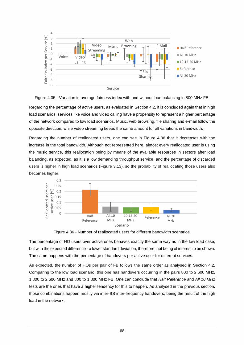
68
Figure 4.35 - Variation in average fairness index with and without load balancing in 800 MHz FB.
Regarding the percentage of active users, as evaluated in Section 4.2, it is concluded again that in high
load scenarios, services like voice and video calling have a propensity to represent a higher percentage
of the network compared to low load scenarios. Music, web browsing, file sharing and e-mail follow the
opposite direction, while video streaming keeps the same amount for all variations in bandwidth.
Regarding the number of reallocated users, one can see in Figure 4.36 that it decreases with the
increase in the total bandwidth. Although not represented here, almost every reallocated user is using
the music service, this reallocation being by means of the available resources in sectors after load
balancing, as expected, as it is a low demanding throughput service, and the percentage of discarded
users is higher in high load scenarios (Figure 3.13), so the probability of reallocating those users also
becomes higher.
Figure 4.36 - Number of reallocated users for different bandwidth scenarios.
The percentage of HO users over active ones behaves exactly the same way as in the low load case,
but with the expected difference - a lower standard deviation, therefore, not being of interest to be shown.
The same happens with the percentage of handovers per active user for different services.
As expected, the number of HOs per pair of FB follows the same order as analysed in Section 4.2.
Comparing to the low load scenario, this one has handovers occurring in the pairs 800 to 2 600 MHz,
1 800 to 2 600 MHz and 800 to 1 800 MHz FB. One can conclude that Half Reference and All 10 MHz
tests are the ones that have a higher tendency for this to happen. As analysed in the previous section,
those combinations happen mostly via inter-BS inter-frequency handovers, being the result of the high
load in the network.
-6
-5
-4
-3
-2
-1
0
1
2
3
4
Fair
nes
s In
dex
per
Ser
vice
[%
]
Service
Half Reference
All 10 MHz
10-15-20 MHz
Reference
All 20 MHz
Voice Video Calling
Video Streaming
Music
Web Browsing
FileSharing
0
0.05
0.1
0.15
0.2
0.25
0.3
Rea
lloca
ted
use
rs p
er
acti
ve u
ser
[%]
All 20 MHz
Half Reference
Scenario
ReferenceAll 10 MHz
10-15-20MHz
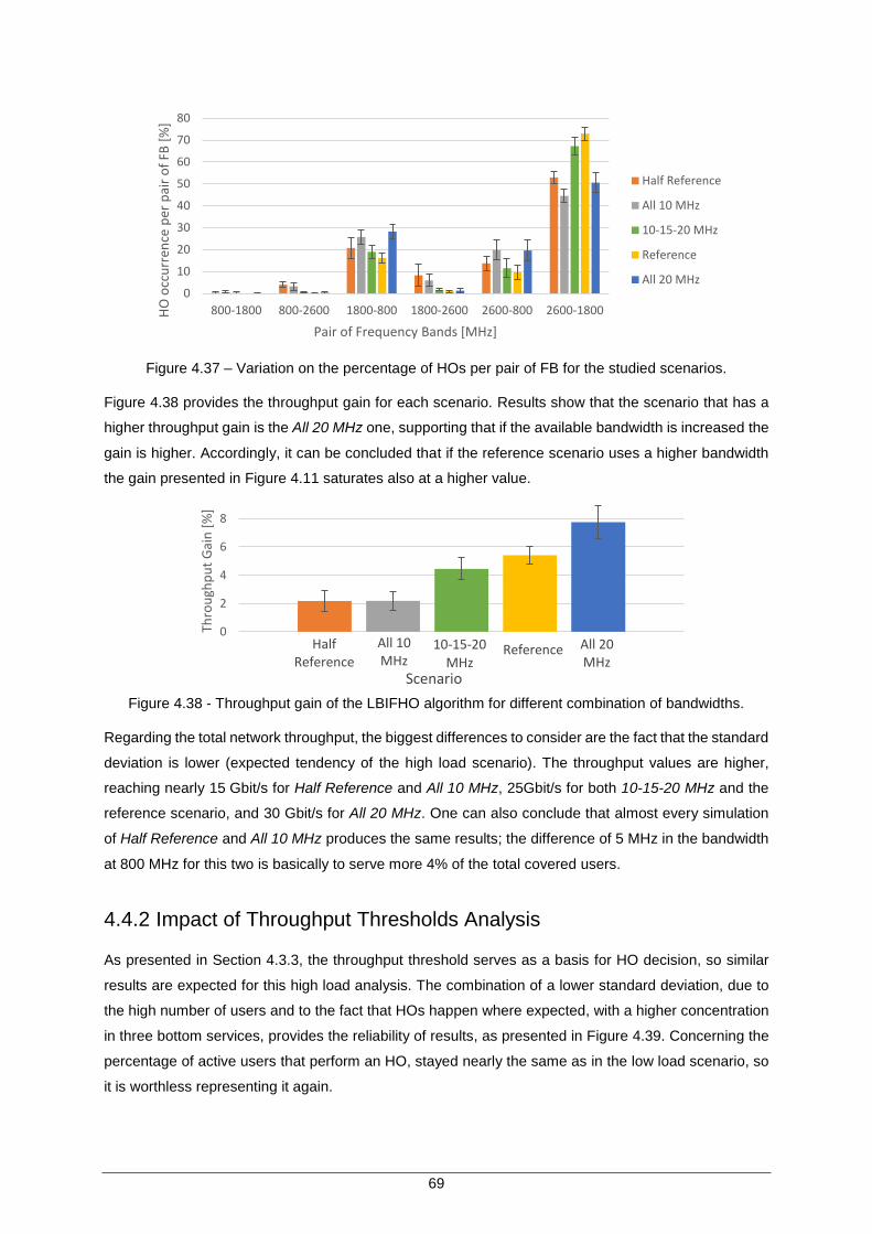
69
Figure 4.37 – Variation on the percentage of HOs per pair of FB for the studied scenarios.
Figure 4.38 provides the throughput gain for each scenario. Results show that the scenario that has a
higher throughput gain is the All 20 MHz one, supporting that if the available bandwidth is increased the
gain is higher. Accordingly, it can be concluded that if the reference scenario uses a higher bandwidth
the gain presented in Figure 4.11 saturates also at a higher value.
Figure 4.38 - Throughput gain of the LBIFHO algorithm for different combination of bandwidths.
Regarding the total network throughput, the biggest differences to consider are the fact that the standard
deviation is lower (expected tendency of the high load scenario). The throughput values are higher,
reaching nearly 15 Gbit/s for Half Reference and All 10 MHz, 25Gbit/s for both 10-15-20 MHz and the
reference scenario, and 30 Gbit/s for All 20 MHz. One can also conclude that almost every simulation
of Half Reference and All 10 MHz produces the same results; the difference of 5 MHz in the bandwidth
at 800 MHz for this two is basically to serve more 4% of the total covered users.
4.4.2 Impact of Throughput Thresholds Analysis
As presented in Section 4.3.3, the throughput threshold serves as a basis for HO decision, so similar
results are expected for this high load analysis. The combination of a lower standard deviation, due to
the high number of users and to the fact that HOs happen where expected, with a higher concentration
in three bottom services, provides the reliability of results, as presented in Figure 4.39. Concerning the
percentage of active users that perform an HO, stayed nearly the same as in the low load scenario, so
it is worthless representing it again.
0
10
20
30
40
50
60
70
80
800-1800 800-2600 1800-800 1800-2600 2600-800 2600-1800HO
occ
urr
ence
per
pai
r o
f FB
[%
]
Pair of Frequency Bands [MHz]
Half Reference
All 10 MHz
10-15-20 MHz
Reference
All 20 MHz
0
2
4
6
8
Thro
ugh
pu
t G
ain
[%
]
All 20 MHz
Half Reference
Scenario
ReferenceAll 10 MHz
10-15-20
MHz
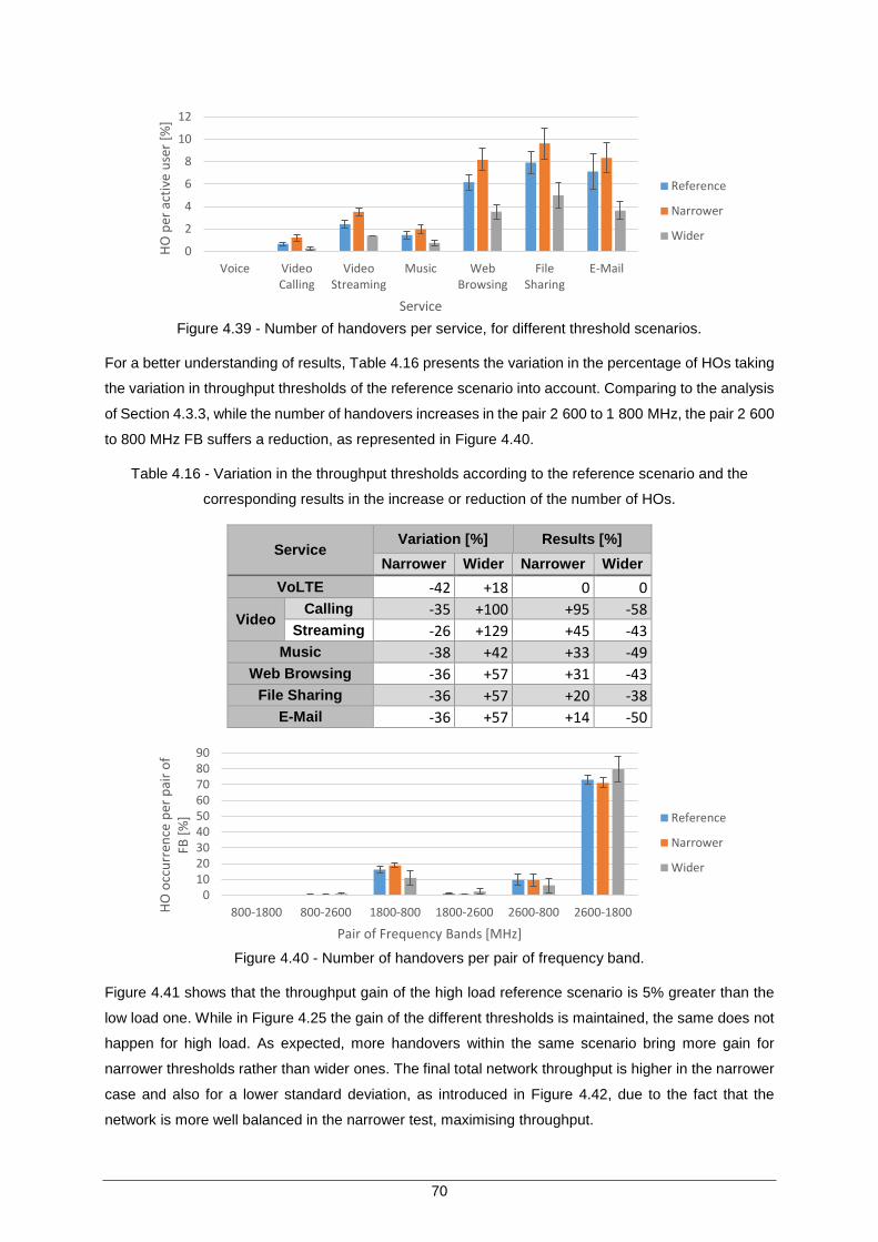
70
Figure 4.39 - Number of handovers per service, for different threshold scenarios.
For a better understanding of results, Table 4.16 presents the variation in the percentage of HOs taking
the variation in throughput thresholds of the reference scenario into account. Comparing to the analysis
of Section 4.3.3, while the number of handovers increases in the pair 2 600 to 1 800 MHz, the pair 2 600
to 800 MHz FB suffers a reduction, as represented in Figure 4.40.
Table 4.16 - Variation in the throughput thresholds according to the reference scenario and the
corresponding results in the increase or reduction of the number of HOs.
Service Variation [%] Results [%]
Narrower Wider Narrower Wider
VoLTE -42 +18 0 0
Video Calling -35 +100 +95 -58
Streaming -26 +129 +45 -43
Music -38 +42 +33 -49
Web Browsing -36 +57 +31 -43
File Sharing -36 +57 +20 -38
E-Mail -36 +57 +14 -50
Figure 4.40 - Number of handovers per pair of frequency band.
Figure 4.41 shows that the throughput gain of the high load reference scenario is 5% greater than the
low load one. While in Figure 4.25 the gain of the different thresholds is maintained, the same does not
happen for high load. As expected, more handovers within the same scenario bring more gain for
narrower thresholds rather than wider ones. The final total network throughput is higher in the narrower
case and also for a lower standard deviation, as introduced in Figure 4.42, due to the fact that the
network is more well balanced in the narrower test, maximising throughput.
0
2
4
6
8
10
12
Voice VideoCalling
VideoStreaming
Music WebBrowsing
FileSharing
HO
per
act
ive
use
r [%
]
Service
Reference
Narrower
Wider
0102030405060708090
800-1800 800-2600 1800-800 1800-2600 2600-800 2600-1800HO
occ
urr
ence
per
pai
r o
f FB
[%
]
Pair of Frequency Bands [MHz]
Reference
Narrower
Wider
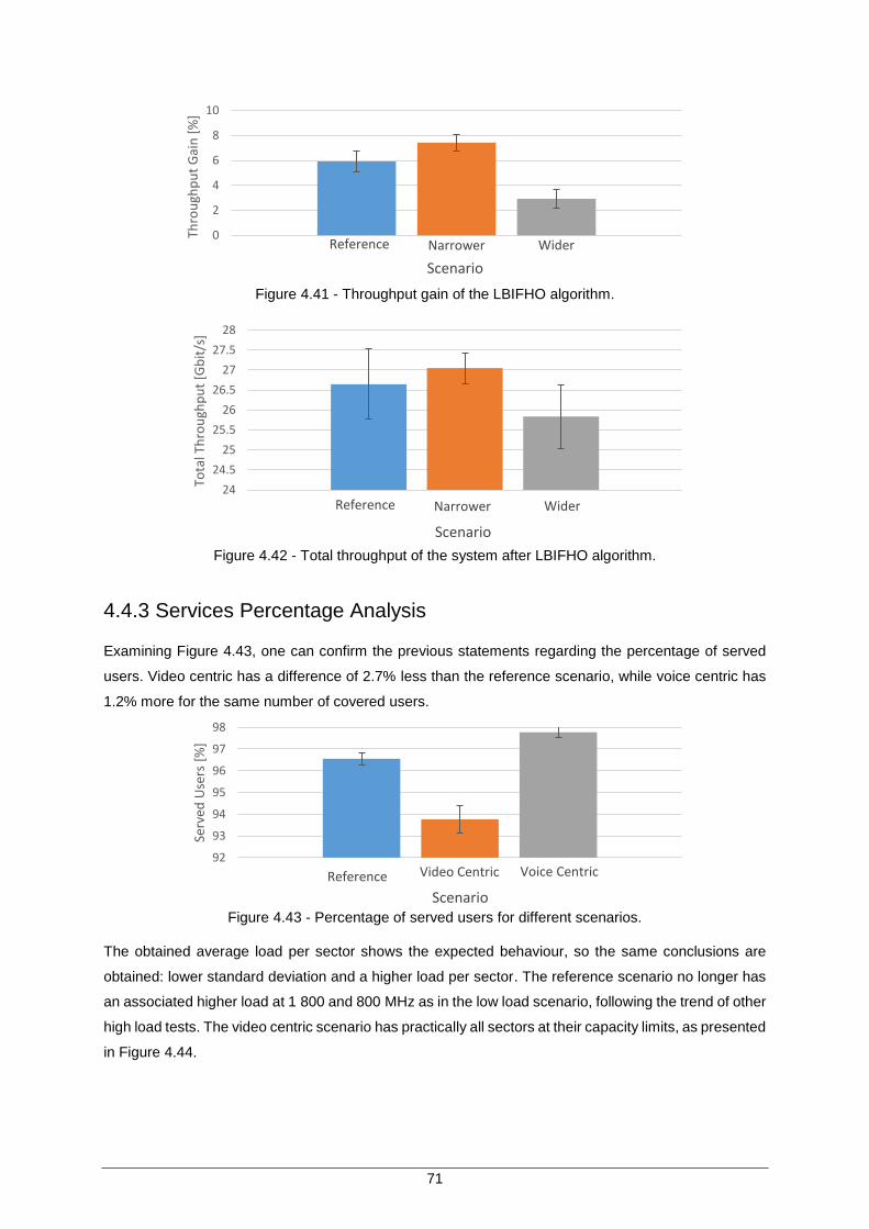
71
Figure 4.41 - Throughput gain of the LBIFHO algorithm.
Figure 4.42 - Total throughput of the system after LBIFHO algorithm.
4.4.3 Services Percentage Analysis
Examining Figure 4.43, one can confirm the previous statements regarding the percentage of served
users. Video centric has a difference of 2.7% less than the reference scenario, while voice centric has
1.2% more for the same number of covered users.
Figure 4.43 - Percentage of served users for different scenarios.
The obtained average load per sector shows the expected behaviour, so the same conclusions are
obtained: lower standard deviation and a higher load per sector. The reference scenario no longer has
an associated higher load at 1 800 and 800 MHz as in the low load scenario, following the trend of other
high load tests. The video centric scenario has practically all sectors at their capacity limits, as presented
in Figure 4.44.
0
2
4
6
8
10
Thro
ugh
pu
t G
ain
[%
]
WiderNarrowerReference
Scenario
24
24.5
25
25.5
26
26.5
27
27.5
28
Tota
l Th
rou
ghp
ut
[Gb
it/s
]
WiderNarrowerReference
Scenario
92
93
94
95
96
97
98
Serv
ed U
sers
[%
]
Voice CentricVideo CentricReference
Scenario
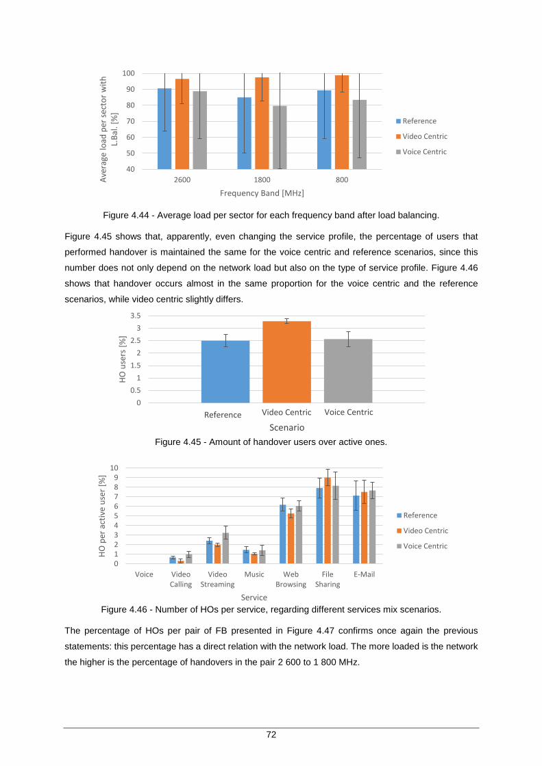
72
Figure 4.44 - Average load per sector for each frequency band after load balancing.
Figure 4.45 shows that, apparently, even changing the service profile, the percentage of users that
performed handover is maintained the same for the voice centric and reference scenarios, since this
number does not only depend on the network load but also on the type of service profile. Figure 4.46
shows that handover occurs almost in the same proportion for the voice centric and the reference
scenarios, while video centric slightly differs.
Figure 4.45 - Amount of handover users over active ones.
Figure 4.46 - Number of HOs per service, regarding different services mix scenarios.
The percentage of HOs per pair of FB presented in Figure 4.47 confirms once again the previous
statements: this percentage has a direct relation with the network load. The more loaded is the network
the higher is the percentage of handovers in the pair 2 600 to 1 800 MHz.
40
50
60
70
80
90
100
2600 1800 800Ave
rage
load
per
sec
tor
wit
h
L.B
al. [
%]
Frequency Band [MHz]
Reference
Video Centric
Voice Centric
0
0.5
1
1.5
2
2.5
3
3.5
HO
use
rs [
%]
Voice CentricVideo CentricReference
Scenario
0123456789
10
Voice VideoCalling
VideoStreaming
Music WebBrowsing
FileSharing
HO
per
act
ive
use
r [%
]
Service
Reference
Video Centric
Voice Centric
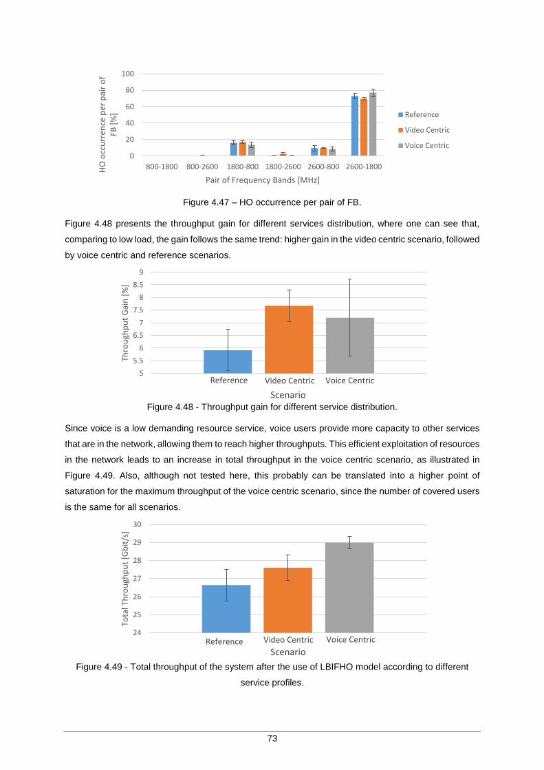
73
Figure 4.47 – HO occurrence per pair of FB.
Figure 4.48 presents the throughput gain for different services distribution, where one can see that,
comparing to low load, the gain follows the same trend: higher gain in the video centric scenario, followed
by voice centric and reference scenarios.
Figure 4.48 - Throughput gain for different service distribution.
Since voice is a low demanding resource service, voice users provide more capacity to other services
that are in the network, allowing them to reach higher throughputs. This efficient exploitation of resources
in the network leads to an increase in total throughput in the voice centric scenario, as illustrated in
Figure 4.49. Also, although not tested here, this probably can be translated into a higher point of
saturation for the maximum throughput of the voice centric scenario, since the number of covered users
is the same for all scenarios.
Figure 4.49 - Total throughput of the system after the use of LBIFHO model according to different
service profiles.
0
20
40
60
80
100
800-1800 800-2600 1800-800 1800-2600 2600-800 2600-1800HO
occ
urr
ence
per
pai
r o
f FB
[%
]
Pair of Frequency Bands [MHz]
Reference
Video Centric
Voice Centric
5
5.5
6
6.5
7
7.5
8
8.5
9
Thro
ugh
pu
t G
ain
[%
]
Voice CentricVideo CentricReference
Scenario
24
25
26
27
28
29
30
Tota
l Th
rou
ghp
ut
[Gb
it/s
]
Voice CentricVideo CentricReferenceScenario

74

75
Chapter 5
Conclusions
5 Conclusions
This chapter summarises the work carried out in the thesis, and the main conclusions are presented. In
the end, a few recommendations are given for the development of future work.
76
The main purpose of this thesis was to study the load distribution via inter-frequency handovers in an
LTE network deployed over an urban scenario in order to maximise network capacity, always ensuring
QoS. To accomplish this goal, a model was developed and implemented into a simulator, several
simulations being performed, to analyse the impact of different load conditions, bandwidths, throughput
thresholds as well as services percentages on network performance.
The first chapter provides a brief overview on mobile communication evolution over time, addressing
different kind of services demands, followed by the motivation and contents that lead to the developing
of this thesis.
Chapter 2 focuses on describing the fundamental concepts of LTE networks, concerning network
architecture, radio interface, coverage and capacity aspects, and service and applications. Data rate
strongly decreases with the reduction of SNR/SINR conditions. One also presents a description of some
traffic services, with respective priorities and throughputs demands to be further used in the developed
model. At the end of this chapter, a state of the art is provided, presenting some of the previously
developed works that approach load balancing techniques. Nokia found in 2002 that the introduction of
load based HO thresholds leads to a decrease in HO measurements and signalling, as well as in
reducing the ping-pong effect. In 2006, S. Moiseev et al. compared an SNR based with an SNR QoS
based load balancing method, and concluded that the sector load using the second method was stable
during the whole simulation time. In 2009, Ericsson evaluated the criteria for IFHO decision based on
RSRP, RSRQ and a combination of the two, concluding that the best scenario occurs with the utilisation
of RSRQ plus RSRP, which leads to a lower number of IFHOs.
Chapter 3 provides a full description of the developed model, as well as the simulator that implements
it. The model and the simulator address in the most realistic way possible the behaviour of an LTE
network, taking aspects such as SNR, cell load, and different population density according to the city
district. The association of users to sectors is based on received power (SNR), and not only on distance
to the BS. The received power is calculated by using the link budget provided in Annex A, which
considers a slow fading margin as a fixed value. Path loss is computed according to the COST-231
Walfisch-Ikegami model, provided in Annex B. The calculations for antenna gain are based on 3GPP
models for horizontal and vertical radiation patterns, which enable shaping the coverage areas of each
FB according to the deployment of a real network. Expressions for throughput calculation of each UE
are introduced in Annex C. The simulator is based on an implementation developed in previous Master
theses, the possibility of having three frequency bands connected at the same time having been
developed in this thesis, together with many other changes: all the process of load calculation was
implemented from scratch, satisfying different service demands and taking the load of each sector into
account; load balancing via inter-frequency handovers was implemented to allow IFHO inter-BS and
intra-BS. In the last part of the chapter, the model assessment is provided, confirming that high priority
services, like VoLTE or video calling are the ones that have always high QoS standards opposed to low
priority services that suffer a decrease in QoS in high load environments. It is important to note that the
traffic studied under the scope of this thesis is only in downlink.
Chapter 4 begins with a description of the reference scenario, containing all the parameters used in the
77
simulator, as well as the list of input and output parameters to be further analysed. The three frequency
bands that were considered, are the ones used by Portuguese mobile operators in LTE (800, 1 800 and
2 600 MHz). Each of them has an associated bandwidth that usually depends on the carrier frequency,
in this case, 10, 20 and 20 MHz respectively. A dense urban scenario for the entire environment of the
city of Lisbon was considered. The results analysis includes the variation of the number of users in the
network, different combinations of bandwidths and throughput thresholds, and finally the variation in the
service mix for low and high load scenarios.
In the analysis on the impact of the number of users on the network, two simulations were performed
for each number of users, since a single sweep takes about a week to perform, due to MapInfo making
use of only one CPU core at time, leading to a poor statistical relevance for this analysis. Apart of that,
one can draw some conclusions from the obtained data. When the number of users increases the cell
load also increases, as the average throughput of each service follows the opposite trend. Services like
video streaming occupies about 40% of the total network traffic whatever the load conditions. It is also
concluded that 2 600 MHz is the band that has more connected users (on average). In fact, almost 65%
of the active users are connected to this FB, while 22% are in 1 800 MHz and 13% in 800 MHz (on
average). This comes from the fact that 2 600 MHz has not only more active sectors and a coverage
area very similar to 1 800 MHz, but also because is the first to be which users are assigned.
Nevertheless, 800 MHz is the first to saturate, due to the high coverage area and low capacity, while
1 800 MHz is always slightly the less loaded. The curve of the percentage of users that perform IFHO
has a Gaussian distribution, due to the relation between users that need to be handover and the ones
that can be reduced. The majority of handovers take place from 2 600 to 1 800 MHz, in e-mail, file
sharing and web-browsing services due to Non-GBR and low priority demands. It was also verified that
load balancing methods should be applied for a high number of users, in this scenario from around
6 000, where the throughput gain is maximised.
Then, a low load analysis follows, where a scenario with 1 270 covered users was chosen. Active users
correspond to the number of instant users to whom the network is allocating resources. Since voice is
coded in 20 ms, the real number of served users is different, and so is the real service profile. Five
scenarios were compared, each one having an associated bandwidth combination for each band; Half
Reference for 5, 10 and 10 MHz, All 10 MHz for 10, 10 and 10 MHz and so on. Varying the bandwidth
of each FB does not have an impact on the percentage of served users, maintained at 100%. The same
does not happen with the average load per sector, which decreases with the increase in the available
bandwidth. As the bandwidth is the only changed parameter, one can assume that the number of users
that need to be handover is the same. Therefore, more handovers will happen in scenarios with a higher
capacity, since more users can be reduced. Since this scenario has a low number of users, HOs occur
relatively in the same number for video streaming, web-browsing, file sharing, and e-mail. The
throughput gain is maintained, since the number of active users also remains the same, contrary to what
happens with the total network throughput, where the difference of 25 MHz bandwidth between 10-15-
20 MHz and All 10MHz cases results in almost the double throughput.
Concerning the variation of throughput thresholds, as expected, it was verified that it impacts essentially
78
on the percentage of users that perform IFHO, while other values are maintained relatively unchanged.
Narrower thresholds result in 3% of IFHO users over active ones, while wider values only reach 1.5%.
It is important to note that besides keeping the same trend as in the previous analysis, IFHO occurrence
per pair of FB with wider values seem to have a higher incidence of IFHOs in the pair 2 600 to 1 800 MHz
FB. One can conclude that not only the load influences IFHO occurrence, but also throughput
thresholds.
A comparison was done in between the reference service profile and the ones proposed by [10] (Video
Centric) and [11] (Voice Centric). Video streaming is one of the most demanding resource services,
since it has high priority and maximum throughput, therefore, the sectors load is much higher compared
to voice centric case. The video centric case has the highest load as well as the highest percentage of
users that perform handovers, therefore, it is concluded that the service profile also influences this output
parameter. Regarding system throughput gain, since there are more users demanding IFHO in the video
centric scenario, there is a higher gain for this case. This gain depends on several factors and not only
on the number of HOs, as the conditions on the network and where users are generated.
In the high load scenario, the analysis was done regarding an average of 12 600 covered users, about
a factor of ten to the low load scenario. The percentage of served users increases with the available
bandwidth. Results show that variations at 800 MHz have more impact in this percentage, since it allows
more users at 800 MHz that cannot be in handover to other FBs. The increase on average load per
sector is in the order of 28% at 2 600 MHz, 13% at 1 800 MHz and 16% at 800 MHz, so it means that
2 600 MHz is the first to reach saturation point. Since there is a higher incidence of HOs in the pair of
2 600 to 1 800 MHz, followed by 1 800 to 800 MHz and then 2 600 to 800 MHz FBs, the frequency band
that is more loaded with this model is 800 MHz. In fact, results show that the load in this FB increases
after the use of LBIFHO; in addition, users that are already connected to this FB will be reduced.
Consequently, the FI at 800 MHz was studied after the implementation of LBIFHO. Results show that
even with these constraints, the model provides high standards of fairness among users. Voice users
do not suffer HOs, so the fairness index for this service is maintained the same; on other hand, web
browsing, file sharing and e-mail vary a lot, while video calling users become more equally distributed.
Regarding the number of reallocated users, in the best case scenario, it reaches 0.2%, which is very
low, so it is concluded that it does not increase simulation time and complexity. Throughput gain
increases in all cases, compared to the low load scenario, with All 20 MHz reaching up to 8% gain. In
all other studied parameters, the main differences to consider are the fact that standard deviation is
lower due to the higher number of samples.
Concerning throughput thresholds, the high load scenario brings not only a lower standard deviation in
tests, but also the fact that handovers happen where expected, with a higher concentration in web-
browsing, file sharing and e-mail services. Associated with this, the percentage of HOs in the pair 2 600
to 1 800 MHz increases, while the other two decrease, since in the high load scenario the 800 MHz
band is almost fully occupied, and there are few users with a served throughput higher than the high
threshold. While the gain and total system throughput from using the presented load balancing model is
maintained in low load, the same does not happen in the high load scenario, with a difference of 4% in
79
gain and 1.2 Gbit/s in the total throughput between narrower and wider cases.
High load conditions bring some changes in the percentage of served users for different service profiles,
with video centric serving only 93.8% of the total covered users, while voice centric reaches 98.8%. In
fact, associated with these conditions, comes an overloaded network in the video centric scenario. By
evaluating the results on the percentage of IFHO users, one can confirm that this parameter also
depends on the service profile. The percentage of IFHO per pair of FB behaves proportionally to the
network load.
Although a real wireless communications system is far more complex than the one analysed in this
simulator, results show a good approximation to the real world. In fact, the terrain profile of the city, the
difference between buildings heights and street widths, the need for some BS not to have all three
sectors connected, among other things, were not considered. The presented load balancing model
brings some benefits to the overall network capacity, but on other hand, as the simulator has snapshot
approach, the temporal behaviour was not considered. In order to obtain a full benefit of the simulator,
it is important to take not only the temporal factor in account, but also the fact that constant load
balancing methods can have unwanted effects, since signalling can overload the network.
For future work, an even more realistic scenario could be applied. The main limitation of this thesis
remains in the fact that it does not take interference coming from adjacent cells into account. As
previously described, the inter-cell interference model provided by [10] is available as an option to be
turned on in the simulator, but the main constraint of this model is that it only serves as a calculation for
the final throughput of the UE after all the process of load balancing is completed. An interesting study
to be done is to take SINR into account, making sure that the final configuration of the network is the
most realistic possible. In a real LTE network, the UE is the one responsible for executing the measures
of the received signal quality, so this study is definitely a good choice to be considered in future work.
Traffic is usually unpredictable and highly time-variant, so a simulator that can emulate the real
behaviour of an LTE network, taking traffic variations according to the hour of the day and the size of
data packages for each service, is more than relevant for an operator. Although this study is important,
it takes a lot of effort to be done, so possibly this can only be relevant for a Ph.D. work.
With the increase in the number of connected devices and mobile subscribers, the way that users exploit
mobile networks’ services has changed. Today, the asymmetry between DL and UL is reduced; in fact,
with the emergence of cloud-enabled technologies, the convergence of internet-of-things systems,
social networking and many other services, UL traffic is following a growing trend. Although this thesis
addresses only DL, it is important to understand if and how mobile networks cope with challenging UL
traffic loads.
Finally, another analysis that could be done in order to validate (or not) the need of balancing the network
via inter-frequency handovers involves LTE-Advanced, which allows carrier aggregation as a way to
provide better throughputs for the terminal, by means of aggregating multiple carriers and increasing
the maximum bandwidth. Thus, at a first sight, it could bring some performance benefits for low load
scenarios, as it enables a greater quality-of-experience for high throughput demanding services.

80
81
Annex A
Radio Link Budget
Annex A Radio Link Budget
This annex presents a brief description of the link budget equations, taking into account propagation
between transmitter and receiver, and its losses.

82
This section is based on the chapter “Propagation Models” of [24] and [10]. To evaluate the propagation
between the terminal and the eNB, all losses and gains of antennas must be taken into account. The
power available at the receiving antenna can be given by:
𝑃𝑟 [dBm] = 𝑃𝐸𝐼𝑅𝑃 [dBm] + 𝐺𝑟 [dBi] − 𝐿𝑝,𝑡𝑜𝑡𝑎𝑙 [dB] (A.1)
where:
𝑃𝐸𝐼𝑅𝑃: Effective Isotropic Radiated Power.
𝐺𝑟: Gain of the receiving antenna.
𝐿𝑝,𝑡𝑜𝑡𝑎𝑙: Path loss.
The EIRP depends on the link. For downlink, it can be defined as:
𝑃𝐸𝐼𝑅𝑃 [dBm] = 𝑃𝑇𝑥 [dBm] − 𝐿𝑐 [dB] + 𝐺𝑡 [dBi] (A.2)
where:
𝑃𝑇𝑥: Transmitter output power.
𝐿𝑐: Losses in the cable between the transmitter and the antenna.
𝐺𝑡: Gain of the transmitting antenna.
For uplink, it is expressed by:
𝑃𝐸𝐼𝑅𝑃 [dBm] = 𝑃𝑇𝑥 [dBm] − 𝐿𝑢 [dB] + 𝐺𝑡 [dBi] (A.3)
where:
𝐿𝑢: Losses due to the user body.
According to [20] the UE antenna gain depends on the type of device and on the frequency band. This
gain can range from -5 dBi up to 10 dBi. Regarding the transmitted power, in DL it can range from 43
up to 48 dBm and in the UL is around 24 dBm.
The power at the receiver for DL is given by:
𝑃𝑅𝑥 [dBm] = 𝑃𝑟 [dBm] − 𝐿𝑢 [dB] (A.4)
where:
𝑃𝑅𝑥: Power at the input of the receiver.
For UL is represented by:
𝑃𝑅𝑥 [dBm] = 𝑃𝑟 [dBm] − 𝐿𝑐 [dB] (A.5)
The average noise power can be represented by the expression defined in [18], by:
𝑃𝑁 [dBm] = −174 + 10 log(𝑁𝑅𝐵×𝐵𝑅𝐵 [Hz]) + 𝐹𝑁 [dBm] (A.6)
where:
𝑁𝑅𝐵: Number of RBs.
83
𝐵𝑅𝐵: Bandwidth of one RB, which is 180 kHz.
𝐹𝑁: Noise figure at the receiver that can take values from 6 up to 11 dB.
Connecting all the contributions for the path loss is extracted the total path loss, calculated by:
𝐿𝑝,𝑡𝑜𝑡𝑎𝑙 [dB] = 𝐿𝑝 [dB] + 𝑀𝑆𝐹 [dB] + 𝑀𝐹𝐹 [dB] (A.7)
where:
𝐿𝑝: Path loss from the COST-231 Walfish-Ikegami model.
𝑀𝑆𝐹: Slow fading margin.
𝑀𝐹𝐹: Fast fading margin.

84
85
Annex B
COST 231 Walfisch-Ikegami Propagation Model
Annex B COST 231 Walfisch-Ikegami Propagation Model
This annex provides a description of the propagation model used to calculate the path loss in a dense
urban environment.
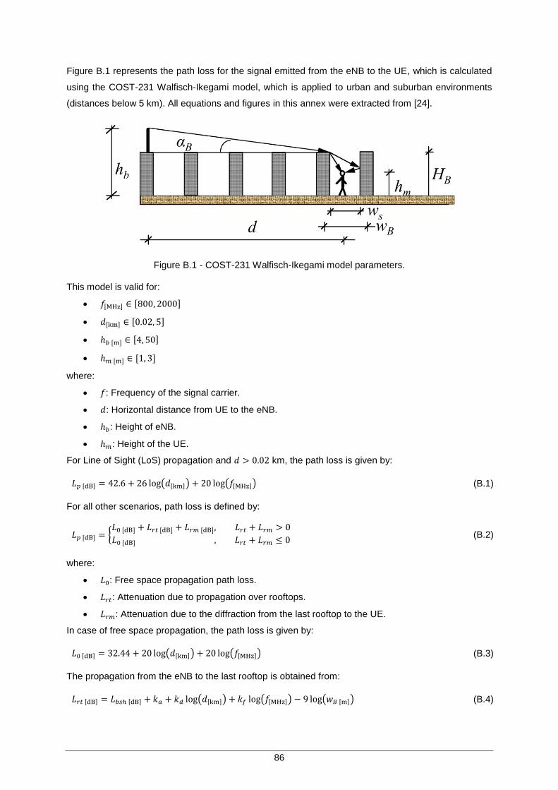
86
Figure B.1 represents the path loss for the signal emitted from the eNB to the UE, which is calculated
using the COST-231 Walfisch-Ikegami model, which is applied to urban and suburban environments
(distances below 5 km). All equations and figures in this annex were extracted from [24].
Figure B.1 - COST-231 Walfisch-Ikegami model parameters.
This model is valid for:
𝑓[MHz] ∈ [800, 2000]
𝑑[km] ∈ [0.02, 5]
ℎ𝑏 [m] ∈ [4, 50]
ℎ𝑚 [m] ∈ [1, 3]
where:
𝑓: Frequency of the signal carrier.
𝑑: Horizontal distance from UE to the eNB.
ℎ𝑏: Height of eNB.
ℎ𝑚: Height of the UE.
For Line of Sight (LoS) propagation and 𝑑 > 0.02 km, the path loss is given by:
𝐿𝑝 [dB] = 42.6 + 26 log(𝑑[km]) + 20 log(𝑓[MHz]) (B.1)
For all other scenarios, path loss is defined by:
𝐿𝑝 [dB] = {𝐿0 [dB] + 𝐿𝑟𝑡 [dB] + 𝐿𝑟𝑚 [dB], 𝐿𝑟𝑡 + 𝐿𝑟𝑚 > 0
𝐿0 [dB] , 𝐿𝑟𝑡 + 𝐿𝑟𝑚 ≤ 0 (B.2)
where:
𝐿0: Free space propagation path loss.
𝐿𝑟𝑡: Attenuation due to propagation over rooftops.
𝐿𝑟𝑚: Attenuation due to the diffraction from the last rooftop to the UE.
In case of free space propagation, the path loss is given by:
𝐿0 [dB] = 32.44 + 20 log(𝑑[km]) + 20 log(𝑓[MHz]) (B.3)
The propagation from the eNB to the last rooftop is obtained from:
𝐿𝑟𝑡 [dB] = 𝐿𝑏𝑠ℎ [dB] + 𝑘𝑎 + 𝑘𝑑 log(𝑑[km]) + 𝑘𝑓 log(𝑓[MHz]) − 9 log(𝑤𝐵 [m]) (B.4)

87
where:
𝐿𝑏𝑠ℎ: Loss due to the height difference between rooftop and the antennas.
𝑤𝐵: Distance between eNB and UE buildings centres.
The loss due to the height difference between rooftop and the antennas is obtained from:
𝐿𝑏𝑠ℎ [dB] = {−18 log(ℎ𝑏 [m] − 𝐻𝐵 [m] + 1) , ℎ𝑏 > 𝐻𝐵
0 , ℎ𝑏 > 𝐻𝐵
(B.5)
where:
𝐻𝐵: Height of the buildings.
Other correction factors are obtained from:
𝑘𝑎 = {
54 , ℎ𝑏 > 𝐻𝐵
54 − 0.8(ℎ𝑏 [m] − 𝐻𝐵 [m]) , ℎ𝑏 ≤ 𝐻𝐵 ⋀ 𝑑 ≥ 0.5km
54 − 1.6(ℎ𝑏 [𝑚] − 𝐻𝐵 [m])𝑑[km] , ℎ𝑏 ≤ 𝐻𝐵 ⋀ 𝑑 < 0.5km
(B.6)
𝑘𝑑 = {
18 , ℎ𝑏 > 𝐻𝐵
18 − 15(ℎ𝑏 [m] − 𝐻𝐵 [m])
𝐻𝐵 [m], ℎ𝑏 ≤ 𝐻𝐵
(B.7)
𝑘𝑓 = {−4 + 07 (
𝑓[MHz]
925− 1) , urban and suburban scenarios
−4 + 1.5 (𝑓[MHz]
925− 1) , dense urban scenarios
(B.8)
The loss due to diffraction from the last rooftop to the UE is given by:
𝐿𝑟𝑚 [dB] = −16.9 − 10 log(𝑤𝑠 [m]) + 10 log(𝑓[MHz]) + 20𝑙𝑜𝑔(𝐻𝐵 [m] − ℎ𝑚 [m]) + 𝐿𝑜𝑟𝑖 [dB] (B.9)
where:
𝑤𝑠: Width of the street.
The loss due to the street orientation is obtained from:
𝐿𝑜𝑟𝑖 [dB] = {
−10 + 0.354𝜙[°] , 0° < 𝜙 < 35°
2.5 + 0.075(𝜙[°] − 35) , 35° ≤ 𝜙 < 55°
4 − 0.114(𝜙[°] − 55) , 55° ≤ 𝜙 ≤ 90°
(B.10)
where:
𝜙: Angle of incidence of the signal in the buildings, on the horizontal plane.
Taking into account that this model does not fulfil all the frequency bands analysed in this thesis, one
should accept that the final results may present some errors. The error increases when ℎ𝑏 decreases
relative to 𝐻𝐵 and the standard deviation takes values in [4, 7] dB.

88
89
Annex C
SNR and Throughput
Annex C SINR and Throughput
This annex provides an overview on the formulas that relate SNR and throughput in LTE for a given set
of system configurations.

90
This annex is based on the formulas provided by [10], in which it was considered three expressions to
relate experienced SNR and throughput. These expressions were derived from the three modulation
types considered in DL, meaning QPSK, 16QAM and 64QAM. They represent the logistic functions
that provide the best-fit approach to a set of values collected by 3GPP on throughput performance
tests done by manufacturers. In order to have a more realistic approach to a real network, were chosen
three MCS associated with the mean values of coding rates:
QPSK with a coding rate of 1/3.
16QAM with a coding rate of 1/2.
64QAM with a coding rate of 3/4.
For 2x2 MIMO, QPSK and coding rate of 1/3, throughput and the corresponding SNR in the DL can be
given by:
𝑅𝑏[bit/s]=
2.34201×10⁶
14.0051 + 𝑒−0.577897 𝜌𝑁[dB]
(C.1)
𝜌𝑁[dB] = −1
0.577897ln (
2.34201×10⁶
𝑅𝑏[bit/s]
− 14.0051) (C.2)
For 2x2 MIMO, 16 QAM and coding rate of 1/2, throughput and the corresponding SNR in the DL can
be given by:
𝑅𝑏[bit/s]=
47613.1
0.0926275 + 𝑒−0.295838 𝜌𝑁[dB]
(C.3)
𝜌𝑁[dB]= −
1
0.295838ln (
47613.1
𝑅𝑏[bit/s]
− 0.0926275) (C.4)
For 2x2 MIMO, 64 QAM and coding rate of 3/4, throughput and the corresponding SNR in the DL can
be given by:
𝑅𝑏[bit/s]=
26405.8
0.0220186 + 𝑒−0.24491 𝜌𝑁[dB]
(C.5)
𝜌𝑁[dB]= −
1
0.24491ln (
26405.8
𝑅𝑏[bit/s]
− 0.0220186) (C.6)
A more pleasant approach of this relation can be translated in a graph, as one can check in Figure C.1.
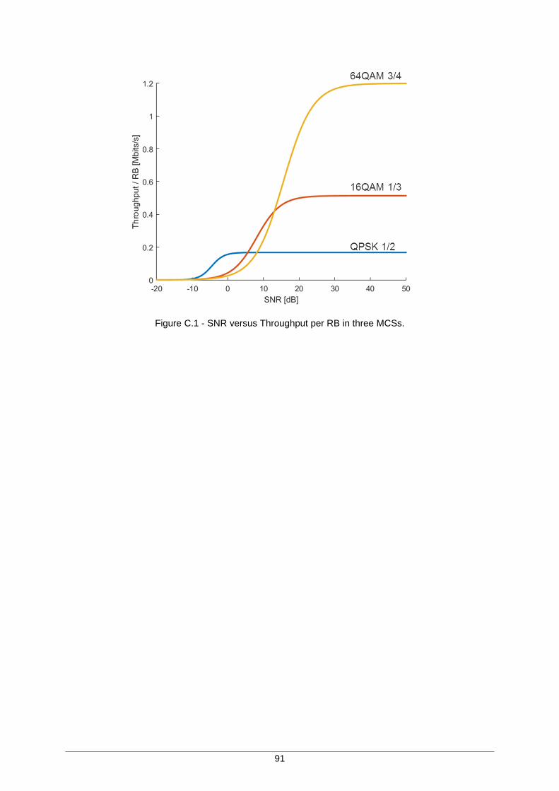
91
Figure C.1 - SNR versus Throughput per RB in three MCSs.

92
93
Annex D
User’s Manual for MapInfo
Annex D User’s Manual for MapInfo
This annex provides an overview of the simulator, along with an explanation on how to run the
simulation.
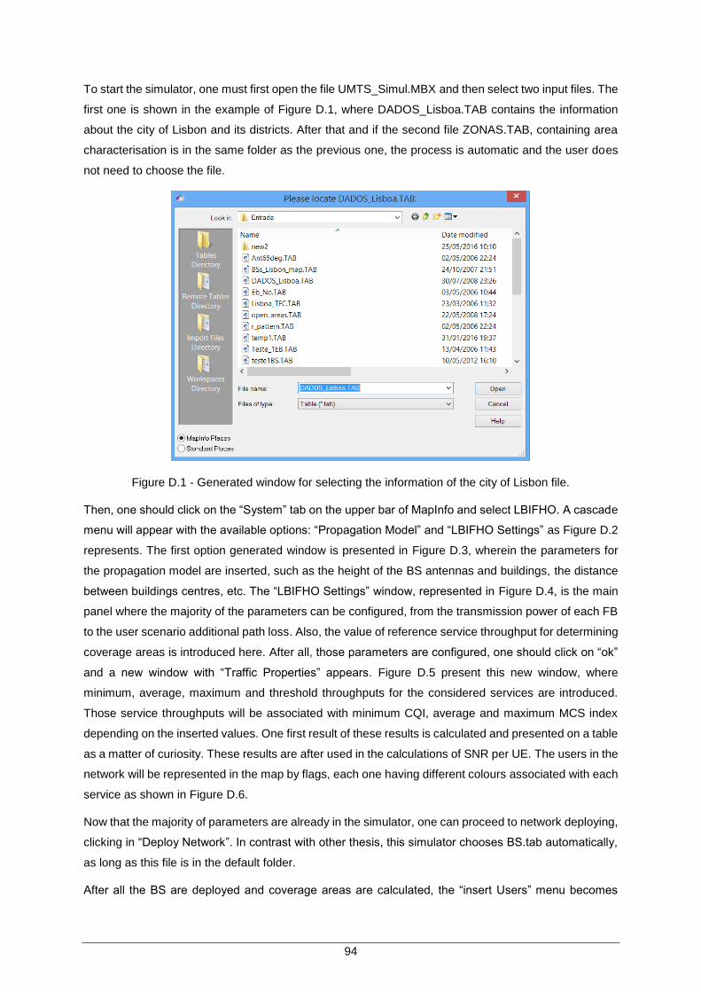
94
To start the simulator, one must first open the file UMTS_Simul.MBX and then select two input files. The
first one is shown in the example of Figure D.1, where DADOS_Lisboa.TAB contains the information
about the city of Lisbon and its districts. After that and if the second file ZONAS.TAB, containing area
characterisation is in the same folder as the previous one, the process is automatic and the user does
not need to choose the file.
Figure D.1 - Generated window for selecting the information of the city of Lisbon file.
Then, one should click on the “System” tab on the upper bar of MapInfo and select LBIFHO. A cascade
menu will appear with the available options: “Propagation Model” and “LBIFHO Settings” as Figure D.2
represents. The first option generated window is presented in Figure D.3, wherein the parameters for
the propagation model are inserted, such as the height of the BS antennas and buildings, the distance
between buildings centres, etc. The “LBIFHO Settings” window, represented in Figure D.4, is the main
panel where the majority of the parameters can be configured, from the transmission power of each FB
to the user scenario additional path loss. Also, the value of reference service throughput for determining
coverage areas is introduced here. After all, those parameters are configured, one should click on “ok”
and a new window with “Traffic Properties” appears. Figure D.5 present this new window, where
minimum, average, maximum and threshold throughputs for the considered services are introduced.
Those service throughputs will be associated with minimum CQI, average and maximum MCS index
depending on the inserted values. One first result of these results is calculated and presented on a table
as a matter of curiosity. These results are after used in the calculations of SNR per UE. The users in the
network will be represented in the map by flags, each one having different colours associated with each
service as shown in Figure D.6.
Now that the majority of parameters are already in the simulator, one can proceed to network deploying,
clicking in “Deploy Network”. In contrast with other thesis, this simulator chooses BS.tab automatically,
as long as this file is in the default folder.
After all the BS are deployed and coverage areas are calculated, the “insert Users” menu becomes
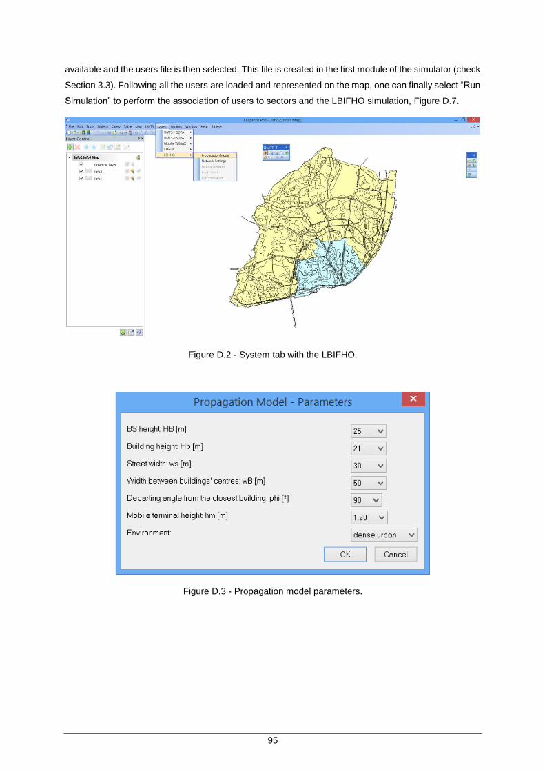
95
available and the users file is then selected. This file is created in the first module of the simulator (check
Section 3.3). Following all the users are loaded and represented on the map, one can finally select “Run
Simulation” to perform the association of users to sectors and the LBIFHO simulation, Figure D.7.
Figure D.2 - System tab with the LBIFHO.
Figure D.3 - Propagation model parameters.
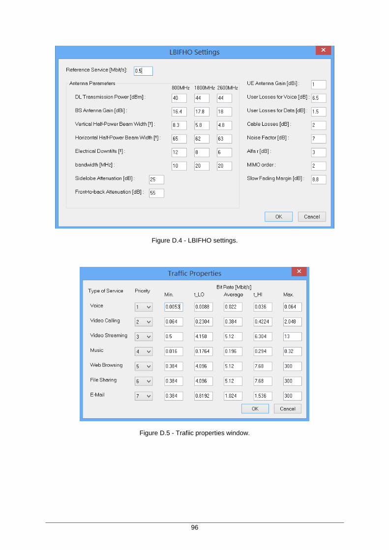
96
Figure D.4 - LBIFHO settings.
Figure D.5 - Trafiic properties window.
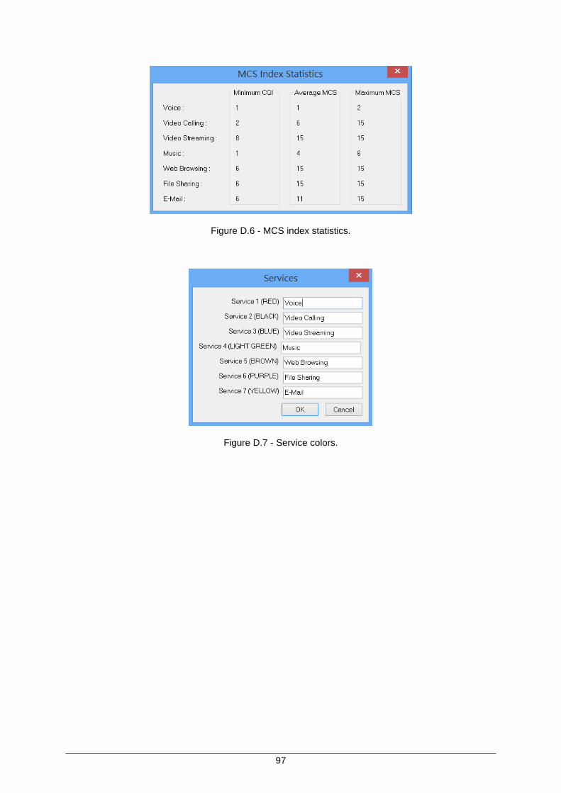
97
Figure D.6 - MCS index statistics.
Figure D.7 - Service colors.

98
99
References
References
[1] S. Ahmadi, LTE-Advanced: A Practical Systems Approach to Understanding 3GPP LTE Releases 10 and 11 Radio Access Technologies, Elsevier, Kidlington, UK, 2014.
[2] Ericsson, Ericsson Mobility Report, Stockholm, Sweden, Nov. 2015 (http://www.ericsson.com/res/docs/2015/mobility-report/ericsson-mobility-report-nov-2015.pdf).
[3] I.F. Akyildiz, D.M. Gutierrez-Estevez, and E.C. Reyes, “The evolution to 4G cellular systems: LTE-Advanced”, Physical Communication, Vol. 3, No. 4, Dec. 2010, pp. 217–244
(http://dx.doi.org/10.1016/j.phycom.2010.08.001).
[4] Cisco, Cisco Visual Networking Index : Global Mobile Data Traffic Forecast Update , 20 5 – 2020 (White Paper), https://www.cisco.com/c/en/us/solutions/collateral/service-provider/visual-networking-index-vni/mobile-white-paper-c11-520862.html, Mar. 2016.
[5] Ericsson, Consumerlab Tv and Media 2015, Stockholm, Sweden, Sep. 2015 (https://www.ericsson.com/res/docs/2015/consumerlab/ericsson-consumerlab-tv-media-2015.pdf).
[6] S.H. Lee and Y. Han, “A Novel Inter-FA Handover Scheme for Load Balancing in IEEE 802.16e System”, in Proc. of VCT’07 - 65th IEEE Vehicular Technology Conference, Dublin, Ireland, Apr.
2007 (http://ieeexplore.ieee.org/lpdocs/epic03/wrapper.htm?arnumber=4212595).
[7] H. Hu, J. Zhang, X. Zheng, Y. Yang, and P. Wu, “Self-configuration and self-optimization for LTE networks”, IEEE Communications Magazine, Vol. 48, No. 2, Feb. 2010, pp. 94–100 (http://ieeexplore.ieee.org/xpl/articleDetails.jsp?arnumber=5402670&newsearch=true&queryText=Self-configuration and self-optimization for LTE networks).
[8] S. Mishra and N. Mathur, Load Balancing Optimization in LTE/LTE-A Cellular Networks: A Review, Amity school of Engineering and Technology, Delhi, Índia, 2014
(http://arxiv.org/abs/1412.7273).
[9] H. Byun and J. Yu, “Automatic handover control for distributed load balancing in mobile communication networks”, Wireless Networks, Vol. 18, No. 1, Jan. 2012, pp. 1–7
(http://www.springerlink.com/index/10.1007/s11276-011-0381-4).
[10] D.X. Almeida, Inter-Cell Interference Impact on LTE Performance in Urban Scenarios, M.Sc.,
Instituto Superior Técnico, Lisboa, Portugal, 2013.
[11] P. Ganço, Load Balancing in Heterogeneous Networks with LTE, M.Sc., Instituto Superior
Técnico, Lisboa, Portugal, 2015.
[12] 3GPP, Overview of 3GPP Release 8, Version 0.3.3, Valbonne, France, Sep. 2014
(http://www.3gpp.org/ftp/Information/WORK_PLAN/Description_Releases/).
[13] T.-T. Tran, Y. Shin, and O.-S. Shin, “Overview of enabling technologies for 3GPP LTE-advanced”, EURASIP Journal on Wireless Communications and Networking, 2012, (p).
[14] Alcatel-Lucent, The LTE Network Architecture - A comprehensive tutorial (White paper), Alcatel-Lucent, Paris, France, 2009 (http://www.cse.unt.edu/~rdantu/FALL_2013_WIRELESS_NETWORKS/LTE_Alcatel_White_Paper.pdf).
[15] F. Capozzi, G. Piro, L. a. Grieco, G. Boggia, and P. Camarda, “Downlink packet scheduling in LTE cellular networks: Key design issues and a survey”, IEEE Communications Surveys and Tutorials, Vol. 15, No. 2, May 2013, pp. 678–700 (http://ieeexplore.ieee.org/xpl/articleDetails.jsp?arnumber=6226795&newsearch=true&queryTe
100
xt=Downlink Packet Scheduling in LTE Cellular Networks: Key Design Issues and a Survey).
[16] A. Ghosh, R. Ratasuk, B. Mondal, N. Mangalvedhe, and T. Thomas, “LTE-advanced: Next-generation wireless broadband technology”, IEEE Wireless Communications, Vol. 17, No. 3, Jun. 2010, pp. 10–22 (http://ieeexplore.ieee.org/xpl/articleDetails.jsp?arnumber=5490974&newsearch=true&queryText=LTE-advanced: Next-generation wireless broadband technology).
[17] G. Berardinelli, L.A. Maestro, S. Frattasi, M.I. Rahman, and P.E. Mogensen, “OFDMA vs. SC-FDMA: Performance Comparison in Local Area IMT-A Scenarios”, IEEE Wireless Communications, Vol. 15, No. 5, Oct. 2008, pp. 64–72 (http://ieeexplore.ieee.org/xpl/articleDetails.jsp?arnumber=4653134&newsearch=true&queryText=OFDMA vs. SC-FDMA: performance comparison in local area imt-a scenarios).
[18] S. Sesia, I. Toufik, and M. Baker, LTE - The UMTS Long Term Evolution: From Theory to Practice, John Wiley & Sons, Ltd, Chichester, UK, 2011.
[19] L. Hanzo, M. Münster, B.J. Choi, and T. Keller, OFDM and MC-CDMA for Broadband Multi-User Communications, WLANs and Broadcasting, John Wiley & Sons, Ltd, Chichester, UK, 2003.
[20] H. Holma and A. Toskala, LTE for UMTS Evolution to LTE-Advanced: Second Edition, John
Wiley & Sons, Ltd, Chichester, UK, 2011.
[21] E. Dahlman, S. Parkvall, and J. Sköld, “LTE Radio Access: An Overview”, 4G: LTE/LTE-Advanced for Mobile Broadband (Second Edition), Elsevier, Berlin, Germany, 2014.
[22] 3GPP, Evolved Universal Terrestrial Radio Access (E-UTRA); Physical channels and modulation, 3GPP TS 36.211, Version 12.7.0, Valbonne, France, Sep. 2015 (http://www.3gpp.org/dynareport/36211.htm).
[23] H. Holma and A. Toskala, LTE for UMTS: OFDMA and SC-FDMA based radio access, John Wiley & Sons, Ltd, Chichester, UK, 2009.
[24] L.M. Correia, Mobile Communication Systems - Course Notes, Instituto Superior Técnico, Lisbon, Portugal, 2014.
[25] M. Iwamura, K. Etemad, M.H. Fong, R. Nory, and R. Love, “Carrier aggregation framework in 3GPP LTE-advanced”, IEEE Communications Magazine, Vol. 48, No. 8, Aug. 2010, pp. 60–67 (http://ieeexplore.ieee.org/xpl/articleDetails.jsp?arnumber=5534588&newsearch=true&queryText=Carrier aggregation framework in 3GPP LTE-advanced [WiMAX/LTE Update]).
[26] ANACOM, Market evaluation of mobile electronic communications under article 39 of the regulation of multiband auction (in Portuguese), Lisbon, Portugal, Aug. 2014 (http://www.anacom.pt/streaming/DecisaoFinal_AvaliacaoMercadoCEMoveis2014.pdf?contentId=1321612&field=ATTACHED_FILE).
[27] ANACOM, Information on multi-band spectrum auction, http://www.anacom.pt/render.jsp?contentId=1106646&languageId=1#.ViUgjvlVhBf, Oct. 2015.
[28] ANACOM, Auction Regulation for the allocation of rights of use of frequencies in the 450 MHz, 800 MHz, 900 MHz, 1800 MHz, 2.1 GHz and 2.6 GHz bands, Lisbon, Portugal, 2011
(http://www.anacom.pt/render.jsp?contentId=1101621#.Vpl2bfmLSWh).
[29] J. Pires, LTE Fixed to Mobile Subscribers QoE evaluation, M.Sc., Instituto Superior Técnico,
Lisboa, Portugal, 2015.
[30] J. Falcão, Inter-Cell Interferences in LTE Radio Networks, M.Sc., Instituto Superior Técnico, Lisbon, Portugal, 2013.
[31] T. Bhat and S. Singh, “Variance based Scheduling to Improve the QoS Performance at the Cell Edge”, in Proc. of IEEE ANTS 2012, Bangalore, India, Aug. 2012
(http://arxiv.org/abs/1208.3085).
[32] J. Salo, M. Nur-Alam, and K. Chang, “Practical Introduction to LTE Radio Planning”, in Proc. of European Communications Engineering (ECE) Ltd, Espoo, Filand, 2010
(http://www.lteexpert.com/lte_rf_wp_16June2013.pdf).
101
[33] L.M. Correia, Mobile Broadband Multimedia Networks: Techniques, models and tools for 4G,
Elsevier, London, UK, 2006.
[34] K. Tassin, LTE and the Internet of Things, Sequans Communications, 2014
(http://www.3gpp.org/news-events/3gpp-news/1607-iot).
[35] Nokia Networks, LTE networks for public safety services, Espoo, Finland, 2014 (http://networks.nokia.com/sites/default/files/document/nokia_lte_for_public_safety_white_paper.pdf).
[36] 3GPP, Technical Specification Group Radio Access, NetworkQuality of Service (QoS) concept and architecture, 3GPP TS 23.107, Version 12.0.0, Valbonne, France, Sep. 2014
(http://www.3gpp.org/DynaReport/23107.htm).
[37] S. Khatibi, Radio Resource Management Strategies in Virtual Networks, Ph.D., Instituto Superior
Técnico, Lisbon, Portugal, 2014.
[38] 3GPP, Technical Specification Group Services and System Aspects; Policy and charging control architecture, 3GPP TS 23.203, Version 13.5.1, Valbonne, France, Sep. 2015
(http://www.3gpp.org/DynaReport/23203.htm).
[39] B. Clerckx, E. Hardouin, D. Mazzarese, S. Nagata, K. Sayana, and D. Lee, LTE Advanced - CoMP | ShareTechnote, http://www.sharetechnote.com/html/LTE_Advanced_CoMP.html, Nov. 2015.
[40] C. Lin, K. Sandrasegaran, X. Zhu, and Z. Xu, “On the performance of capacity integrated CoMP handover algorithm in LTE-Advanced”, in Proc. of 18th Asia Pacific Conference on Communications (APCC), Jeju Island, South Korea, Oct. 2012 (http://ieeexplore.ieee.org/xpl/articleDetails.jsp?arnumber=6388207).
[41] I. Poole, 4G LTE CoMP Tutorial | Coordinated Multipoint, http://www.radio-electronics.com/info/cellulartelecomms/lte-long-term-evolution/4g-lte-advanced-comp-coordinated-multipoint.php, Radio-Electronics.com, Nov. 2015.
[42] 3GPP, Evolved Universal Terrestrial Radio Access (E-UTRA); Requirements for support of radio resource management, 3GPP TS 36.133, Version 13.1.0, Valbonne, France, Oct. 2015
(http://www.3gpp.org/dynareport/36133.htm).
[43] J. Kurjenniemi and T. Henttonen, “Effect of measurement bandwidth to the accuracy of inter-frequency RSRP measurements in LTE”, in Proc. of PIMRC’08 - IEEE 19th International Symposium on Personal, Indoor and Mobile Radio Communications, Cannes, France, Sep. 2008
(http://ieeexplore.ieee.org/lpdocs/epic03/wrapper.htm?arnumber=4699694).
[44] ETSI, LTE; Evolved Universal Terrestrial Radio Access (E-UTRA); Radio Resource Control (RRC); Protocol specification, 3GPP TS 36.331, Version 12.7.0, Valbonne, France, Sep. 2015
(http://www.etsi.org/standards-search).
[45] ETSI, LTE; Evolved Universal Terrestrial Radio Access (E-UTRA); Physical layer - Measurements, 3GPP TS 36.214, Version 12.2.0, Valbonne, France, Mar. 2015 (http://www.3gpp.org/dynareport/36214.htm).
[46] 3GPP, “Clarification of the intra and inter frequency measurement for CA, R4- 3482”, in Proc. of 3GPP TSG-RAN WG4, Bucharest, Romania, Jun. 2011
(http://www.3gpp.org/DynaReport/TDocExMtg--R4-59--28982.htm).
[47] A. ElNashar, M.A. El-saidny, and M.R. Sherif, Design, Deployment and Performance of 4G-LTE Networks: A Practical Approach, John Wiley & Sons, Ltd, Chichester, UK, 2014.
[48] V. Sevindik, J. Wang, O. Bayat, J. Weitzen, J. Wang, and O. Bayat, “Performance evaluation of a real long term evolution (LTE) network”, in Proc. of 37th Annual IEEE Conference on Local Computer Networks -- Workshops, Clearwater, Florida, US, Oct. 2012
(http://ieeexplore.ieee.org/lpdocs/epic03/wrapper.htm?arnumber=6424050).
[49] T. Kashima and H. Zhu, “Load balancing effect of inter-frequency handover with pilot power tuning in UTRAN”, in Proc. of VTC’04 - IEEE 59th Vehicular Technology Conference, Tokyo,
Japan, May 2004 (http://ieeexplore.ieee.org/xpl/articleDetails.jsp?arnumber=1390619).
102
[50] S.N. Moiseev, S.A. Filin, M.S. Kondakov, A. V. Garmonov, A.Y. Savinkov, Y.S. Park, D.H. Yim, J.H. Lee, S.H. Cheon, and K.T. Han, “Load-Balancing QOS-Guaranteed Handover in the IEEE 802. Network”, in Proc. of IEEE 17th International Symposium on Personal Indoor and Mobile Radio Communications, Helsinki, Finland, Sep. 2006
(http://ieeexplore.ieee.org/lpdocs/epic03/wrapper.htm?arnumber=4022300).
[51] M. Kazmi, O. Sjöbergh, W. Müller, J. Wiorek, and B. Lindoff, “Evaluation of inter-frequency quality handover criteria in E-UTRAN”, in Proc. of VTC’09 - IEEE 69th Vehicular Technology Conference, Barcelona, Spain, Apr. 2009.
[52] A. Tolli and P. Hakalin, “Adaptive load balancing between multiple cell layers”, in Proc. of VTC’02 - IEEE 56th Vehicular Technology Conference, Málaga, Spain, 2002
(http://ieeexplore.ieee.org/xpl/articleDetails.jsp?arnumber=1040504).
[53] S. Filin, H. Harada, M. Hasegawa, and S. Kato, “QoS-guaranteed load-balancing dynamic spectrum access algorithm”, in Proc. of PIMRC’08 - IEEE 19th International Symposium on Personal, Indoor and Mobile Radio Communications, Cannes, France, Sep. 2008 (http://ieeexplore.ieee.org/xpl/articleDetails.jsp?arnumber=4699466).
[54] 3GPP, Technical Specification Group Radio Access Network, 3GPP TR 36.814, Version 9.0.0, Valbonne, France, Mar. 2010 (http://www.3gpp.org/dynareport/36814.htm).
[55] O.N.C. Yilmaz, S. Hämäläinen, and J. Hämäläinen, “Comparison of remote electrical and mechanical antenna downtilt performance for 3GPP LTE”, in Proc. of IEEE 70th Vehicular Technology Conference Fall, Anchorage, Alaska, Sep. 2009
(http://ieeexplore.ieee.org/xpl/articleDetails.jsp?arnumber=5379074).
[56] Vodafone, Vodafone is the first operator in Portugal to offer VoLTE, the most advanced 4G voice technology (in Portuguese), http://press.vodafone.pt/2015/09/28/vodafone-e-o-primeiro-operador-em-portugal-a-disponibilizar-volte-a-mais-avancada-tecnologia-de-voz-4g/, Press Releases, May 2016.
[57] Kathrein, 690-6000 Base Station Antennas and Antenna Line Products, Catalogue 2016, Rosenheim, Germany, Feb. 2016 (https://www.kathrein.de/en/mobile-communication/catalogues-and-brochures/).
Related Documents