Balanced vehicular traffic - unice.frbertheli/Page_Web/TrafficFlow2007/...Balanced vehicular traffic • Extended Aw-Rascle-Greenberg model • Characteristic speeds ¾λ 1 = v+ρu'(ρ)

Modeling highway bottlenecks in balanced vehicular traffic

Florian Siebel

Florian Siebel 2

• Balanced vehicular traffic• Coupling conditions at intersections• Modeling highway bottlenecks

Balanced vehicular traffic

Florian Siebel 4

Aw, Rascle, Greenberg model

• Macroscopic model

hyperbolic system of balance lawsreferences:

- A. Aw and M. Rascle (SIAP 2000) - J. Greenberg (SIAP 2001)- M. Zhang (Transportation Research B 2002)

• Motivation for an extensionmulti-valued fundamental diagram

- Greenberg, Klar, Rascle (SIAP 2002)instabilities

- Greenberg (SIAP 2004)instantaneous reaction to the current traffic situation

Tvu

xuvv

tuvxv

t))(()))((()))(((

0)(

−=

∂−∂

+∂−∂

=∂

∂+

∂∂

ρρρρρρ

ρρcontinuity equation:

pseudomomentumequation:

M. Koshi et al (1983)

ρ: vehicle densityv: dynamical velocityu(ρ): equilibrium velocityT>0: relaxation time

Florian Siebel 5

Balanced vehicular traffic

• Extended Aw-Rascle-Greenberg model

• Characteristic speedsλ1 = v+ρu'(ρ) ≤ vλ2 = v

• Effective relaxation coefficient b(ρ,v)ARG: constant, inverse relaxation timehere: function of density ρ and velocity v

• PapersF. Siebel, W. Mauser, SIAP 66, 1150 (2006)F. Siebel, W. Mauser, PRE 73, 066108 (2006)

))((),()))((()))(((

0)(

vuvbxuvv

tuvxv

t

−=∂−∂

+∂−∂

=∂

∂+

∂∂

ρρρρρρρ

ρρ continuity equation

pseudomomentum equation

effective relaxation coefficient b(ρ,v)

Florian Siebel 6

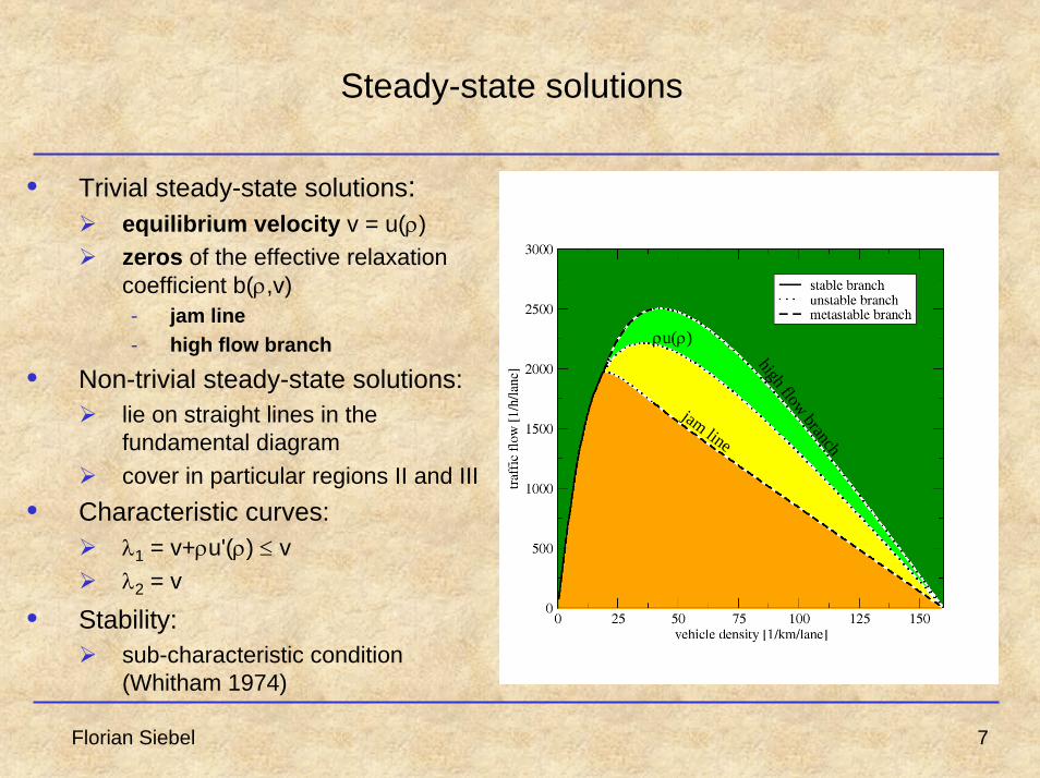
Steady-state solutions

• Trivial steady-state solutions:equilibrium velocity v = u(ρ)zeros of the effective relaxation coefficient b(ρ,v)- jam line- high flow branch

• Non-trivial steady-state solutions: jam line

high flow branch

ρu(ρ)

lie on straight lines in the fundamental diagramcover in particular regions II and III

• Characteristic curves:λ1 = v+ρu'(ρ) ≤ vλ2 = v

Florian Siebel 7

Steady-state solutions

• Trivial steady-state solutions:equilibrium velocity v = u(ρ)zeros of the effective relaxation coefficient b(ρ,v)- jam line- high flow branch

• Non-trivial steady-state solutions: lie on straight lines in the fundamental diagramcover in particular regions II and III

• Characteristic curves:λ1 = v+ρu'(ρ) ≤ vλ2 = v

• Stability:sub-characteristic condition (Whitham 1974)

jam line

high flow branch

ρu(ρ)

Florian Siebel 8

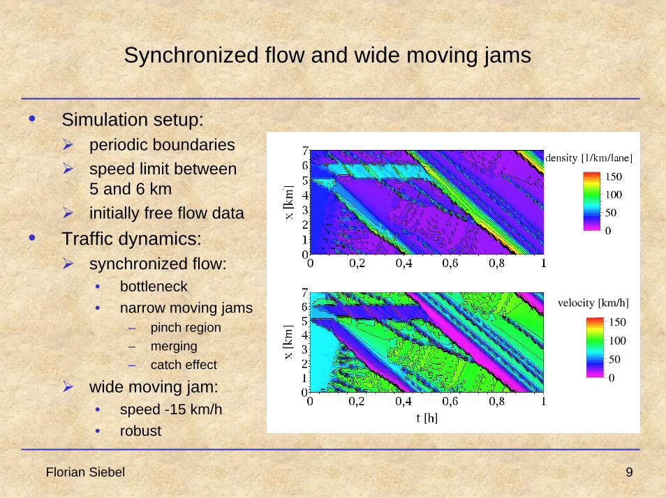
Synchronized flow and wide moving jams

• Simulation setup:periodic boundariesspeed limit between 5 and 6 km

initially free flow data• Traffic dynamics:

synchronized flow:• bottleneck• narrow moving jams

– pinch region– merging– catch effect

wide moving jam:• speed -15 km/h• robust

Florian Siebel 9

Synchronized flow and wide moving jams

• Simulation setup:periodic boundariesspeed limit between 5 and 6 km

initially free flow data• Traffic dynamics:

synchronized flow:• bottleneck• narrow moving jams

– pinch region– merging– catch effect

wide moving jam:• speed -15 km/h• robust

Florian Siebel 10

Synchronized flow and wide moving jams

• Measurements of a virtual detector located at x=0 km:

wide moving jams

narrow moving jams

Coupling conditions at intersections

Florian Siebel 12

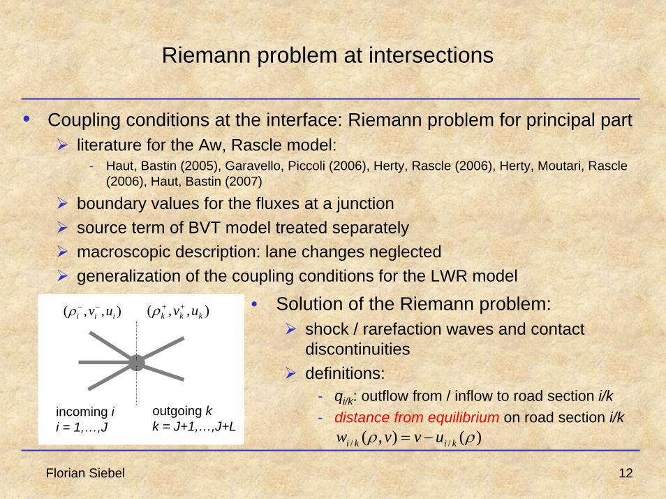
Riemann problem at intersections

• Coupling conditions at the interface: Riemann problem for principal partliterature for the Aw, Rascle model:

- Haut, Bastin (2005), Garavello, Piccoli (2006), Herty, Rascle (2006), Herty, Moutari, Rascle(2006), Haut, Bastin (2007)

boundary values for the fluxes at a junctionsource term of BVT model treated separatelymacroscopic description: lane changes neglectedgeneralization of the coupling conditions for the LWR model

),,( iii uv−−ρ ),,( kkk uv++ρ

incoming ii = 1,…,J

outgoing kk = J+1,…,J+L

• Solution of the Riemann problem:shock / rarefaction waves and contact discontinuities definitions:

- qi/k: outflow from / inflow to road section i/k- distance from equilibrium on road section i/k

)(),( // ρρ kiki uvvw −=

Florian Siebel 13

Principles of the coupling conditions

1) Flow conservation

2) Conservation of pseudomomentum flow (no source term!)

define βik as the portion of the flow on the outgoing road k coming from road i

conservation of pseudomomentum flow

(homogenized distance from equilibrium)

∑∑+

+==

=LJ

Jkk

J

ii qq

11

k

LJ

Jkkii

J

iii wqvwq ∑∑

+

+=

−−

=

=11

),(ρ

kiqqJ

iik

LJ

Jkkiki ∀=∀= ∑∑

=

+

+= 111with ββ

kwvw

qwqvwq

kii

J

iiik

kk

LJ

Jkkii

LJ

Jki

J

iikk

∀=⇒

∀=

−−

=

+

+=

−−+

+= =

∑

∑∑ ∑

),(

),(

1

11 1

ρβ

ρβ

21 ww =

321 www ==

3223113 www =+ ββ

1 2

13

2

2

1

3

Florian Siebel 14

Traffic demand (sending flow) on incoming roads

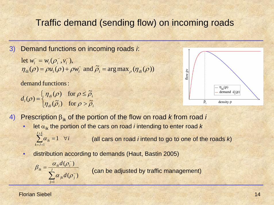
3) Demand functions on incoming roads i:

4) Prescription βik of the portion of the flow on road k from road i• let αik the portion of the cars on road i intending to enter road k

• distribution according to demands (Haut, Bastin 2005)

,),(let −−− = iiii vww ρ

⎩⎨⎧

>≤

=iidi

idiid

ρρρηρρρη

ρ ~for)~(

~for)()(

:functionsdemand

iLJ

Jkik ∀=∑

+

+= 11α (all cars on road i intend to go to one of the roads k)

∑=

−

−

= J

jjjk

iikik

d

d

1)(

)(

ρα

ραβ (can be adjusted by traffic management)

))((maxarg~and)()(di ρηρρρρρη ρ diiii wu =+= −

Florian Siebel 15

Traffic supply (receiving flow) on outgoing roads

5) Supply functions on outgoing roads k:

6) Density on outgoing roads k, where supply function is evaluated:

kksk wu ρρρρη += )()(let

⎩⎨⎧

≤>

=kksk

kskks

ρρρηρρρη

ρ ~for)~(

~for)()(

:functionssupply

+↑↑ ==− kkkkk vvwuv ,)(ofsolution ρρ

))((maxarg~and ρηρ ρ skk =

7) Optimization problemmaximize flow on the outgoing roadsunder the boundary conditions

∑+

+=

LJ

Jkkq

1

max

) roadfor demand totalbyand......supply byboundedroadoutgoingtoflow(

,)(),(min0

demand)byboundedroadincomingfromflow(,)(0

1 kk

kdsq

iidqJ

iiiikkkk

iii

∀⎟⎠

⎞⎜⎝

⎛≤≤

∀≤≤

∑=

−↑

−

ραρ

ρ

Modeling highway bottlenecks

Florian Siebel 17

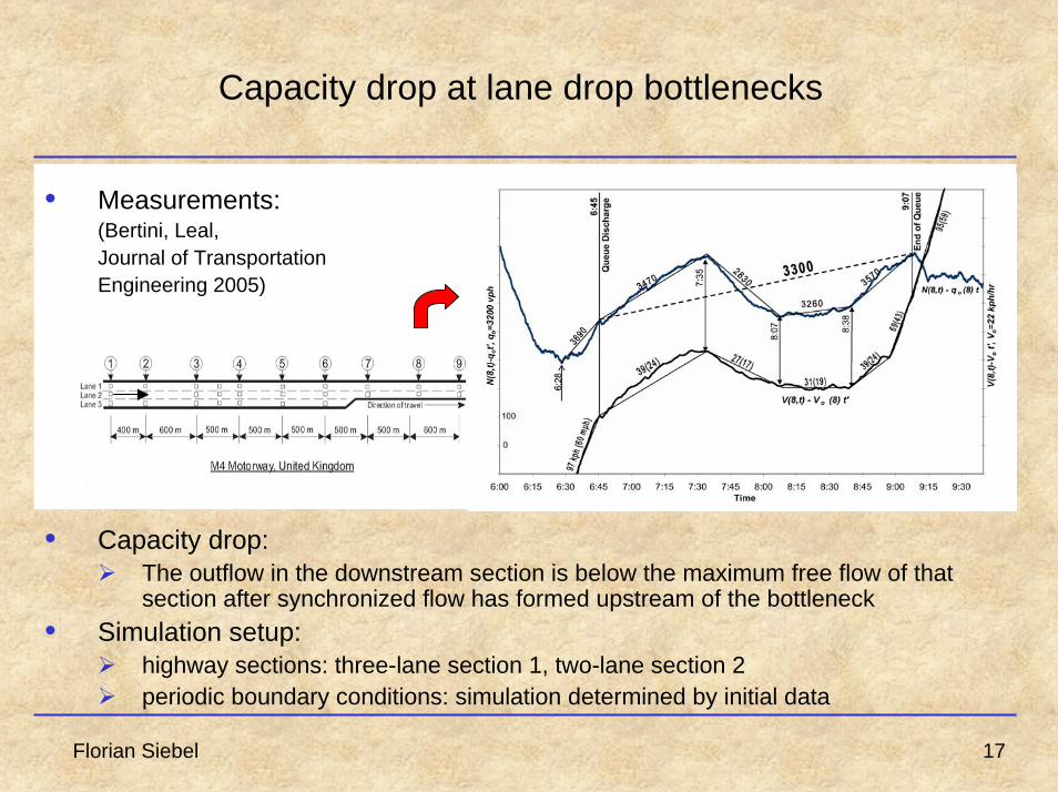
Capacity drop at lane drop bottlenecks

• Measurements:(Bertini, Leal,Journal of Transportation Engineering 2005)

• Capacity drop: The outflow in the downstream section is below the maximum free flow of that section after synchronized flow has formed upstream of the bottleneck

• Simulation setup:highway sections: three-lane section 1, two-lane section 2periodic boundary conditions: simulation determined by initial data

Florian Siebel 18

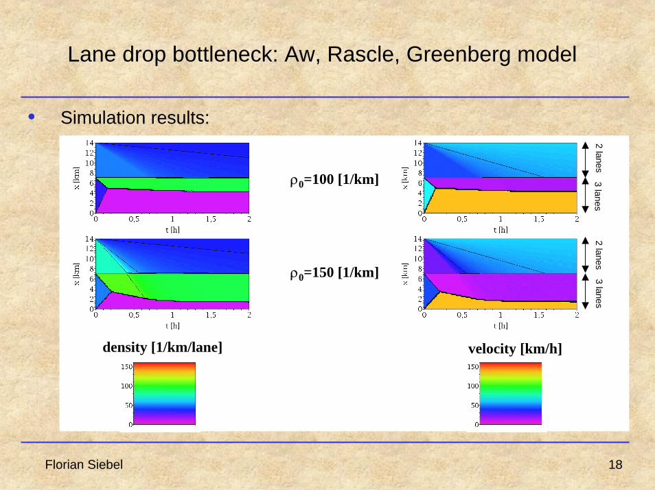
Lane drop bottleneck: Aw, Rascle, Greenberg model

• Simulation results:

density [1/km/lane] velocity [km/h]

ρ0=100 [1/km]

ρ0=150 [1/km] 3 lanes2 lanes

2 lanes3 lanes

Florian Siebel 19

Lane drop bottleneck: Aw, Rascle, Greenberg model

• Static solution:piecewise constant solution with constant total flowshock discontinuity at about 4.2 km and 1.3 km

synchronized flow region in front of the bottleneckmaximum outflow from the bottleneck region in section 2- no capacity drop

Rankine-Hugoniotjump conditions:- flow ρv and

distance from equilibrium w constant across the shock

Florian Siebel 20

Lane drop bottleneck: BVT model

• Simulation results:

density [1/km/lane] velocity [km/h]

ρ0=50 [1/km]

ρ0=100 [1/km] 3 lanes2 lanes

2 lanes3 lanes

Florian Siebel 21

Lane drop bottleneck: BVT model

• Static solution:von Neumann state downstream of the shock, followed by a section of a nontrivial steady-state solution

determined by the crossing of the static solutions with the jam line- similar to wide cluster solutions:

- Zhang, Wong (2006), Zhang, Wong, Dai (2006)

on/off-ramps: - http://arxiv.org/abs/physics/0609237

capacity drop:- flow value

below maximum in downstream section 2

Florian Siebel 22

Conclusion

• Balanced vehicular traffic modelhyperbolic system of balance laws- macroscopic- deterministic- effective one lane- no distinction between different vehicle types- nonlinear dynamics

model results- multi-valued fundamental diagrams- metastability of free flow at the onset of instabilities- wide moving jams- synchronized flow- capacity drop

Michel Rascle, Salissou Moutari, Wolfram Mauser