Bag of Tricks for Long-Tailed Visual Recognition with Deep ...

Bag of Tricks for Long-Tailed Visual Recognition with Deep Convolutional NeuralNetworks

Yongshun Zhang1, Xiu-Shen Wei2,3∗, Boyan Zhou4, Jianxin Wu1

1State Key Laboratory for Novel Software Technology, Nanjing University2PCA Lab, Key Lab of Intelligent Perception and Systems for High-Dimensional Information of Ministry of Education,

School of Computer Science and Engineering, Nanjing University of Science and Technology3Jiangsu Key Lab of Image and Video Understanding for Social Security

4Megvii Research [email protected], {weixs.gm, zhouboyan94, wujx2001}@gmail.com

Abstract

In recent years, visual recognition on challenging long-taileddistributions, where classes often exhibit extremely imbal-anced frequencies, has made great progress mostly based onvarious complex paradigms (e.g., meta learning). Apart fromthese complex methods, simple refinements on training proce-dure also make contributions. These refinements, also calledtricks, are minor but effective, such as adjustments in thedata distribution or loss functions. However, different tricksmight conflict with each other. If users apply these long-tailrelated tricks inappropriately, it could cause worse recognitionaccuracy than expected. Unfortunately, there has not been ascientific guideline of these tricks in the literature. In thispaper, we first collect existing tricks in long-tailed visualrecognition and then perform extensive and systematic ex-periments, in order to give a detailed experimental guidelineand obtain an effective combination of these tricks. Further-more, we also propose a novel data augmentation approachbased on class activation maps for long-tailed recognition,which can be friendly combined with re-sampling methodsand shows excellent results. By assembling these tricks scien-tifically, we can outperform state-of-the-art methods on fourlong-tailed benchmark datasets, including ImageNet-LT andiNaturalist 2018. Our code is open-source and available athttps://github.com/zhangyongshun/BagofTricks-LT.

IntroductionComputer vision has achieved great progress with the devel-opment of convolutional neural networks (CNNs) trained onbalanced distributed datasets (Deng et al. 2009; Krizhevskyand Hinton 2009). But in real-world scenarios, large scaledatasets (Zhou et al. 2017; Van Horn et al. 2018; Lin et al.2014) naturally exhibit the imbalanced and long-tailed distri-butions, where a few categories (majority categories) occupymost of the data while most categories (minority categories)are under-represented. CNNs trained on these long-tailed

∗Corresponding author: X.-S. Wei (Nanjing University of Sci-ence and Technology). This research was supported by NationalNatural Science Foundation of China (No. 61772256, 61921006),the Fundamental Research Funds for the Central Universities (No.30920041111) and CAAI-Huawei MindSpore Open Fund.Copyright c© 2021, Association for the Advancement of ArtificialIntelligence (www.aaai.org). All rights reserved.

datasets deliver poor recognition accuracy, especially forunder-represented minority categories. Dealing with suchlong-tailed distributions is indispensable in real-world appli-cations, such as object detection (Lin et al. 2017; Ouyanget al. 2016), instance segmentation (Wang et al. 2019; Gupta,Dollar, and Girshick 2019), visual recognition (Zhang et al.2017; Cui et al. 2019), etc. In this paper, we focus on thefundamental long-tailed visual recognition problem.

Recently, long-tailed visual recognition has attracted in-creasing attentions. Various methods belonging to differentparadigms, e.g., metric learning (Wang et al. 2018; Cao et al.2019), meta learning (Liu et al. 2019; Peng et al. 2019; Ja-mal et al. 2020) and knowledge transfer (Wang, Ramanan,and Hebert 2017), have been successfully explored. Althoughthese methods bring a steady trend of accuracy improvementson long-tailed datasets, they often suffer from high sensitivityto hyper-parameters (Cao et al. 2019; Yan et al. 2019) or highcomplexity in the training procedures (Wang, Ramanan, andHebert 2017; Liu et al. 2019; Xiang, Ding, and Han 2020). Be-sides, it causes difficulties to efficiently apply these methodsin various real-world scenarios. Apart from these methods,existing training tricks in long-tailed visual recognition alsoplay a major role, which just make simple refinements tothe vanilla training procedure, such as adjustments in lossfunctions or data sampling strategies. These tricks are simplebut make big differences. However, different tricks mighthurt each other during training when they were employedinappropriately. For instance, re-sampling (Buda, Maki, andMazurowski 2018; Japkowicz and Stephen 2002) and re-weighting (Mikolov et al. 2013; Cui et al. 2019) are two com-monly used tricks to alleviate the imbalance of long-taileddistributions. Re-sampling tries to get balanced datasets, andre-weighting assigns weights to categories determined byinversion of class frequencies. Since both re-sampling and re-weighting try to enlarge the influence of minority categories,applying re-weighting and re-sampling simultaneously willobtain similar or even worse accuracy than using them alone.Similar to re-weighting and re-sampling, when we apply twoor more long-tail related tricks, it would be great to knowwhich of them can be combined synergistically and alsowhich of them might conflict with others. Yet, no guidelineis available in the literature. Although there are several good

The Thirty-Fifth AAAI Conference on Artificial Intelligence (AAAI-21)

3447

DatasetsCIFAR-10-LT CIFAR-100-LT

iNaturalist 2018 ImageNet-LTImbalance factor100 50 100 50

Backbones ResNet-32 ResNet-32 ResNet-50 ResNet-10Baseline (Vanilla ResNet) 30.18 24.78 61.73 57.90 39.89 65.99Focal loss (Lin et al. 2017) 29.62 24.75 61.90 57.56 39.70 67.36CB Focal (Cui et al. 2019) 25.43 20.73 60.40 53.79 38.88 –

Feature space augmentation (Chu et al. 2020) – – – – 34.09 64.80Meta-learning (Jamal et al. 2020)† 20.00 17.77 55.92 50.84 32.45 70.10

LDAM with DRW (Cao et al. 2019) 22.97 20.70 57.96 54.92 32.00 63.97Decoupling learning (Kang et al. 2020) – – – – 30.70 58.20

Multi-experts (Xiang, Ding, and Han 2020)†‡ – – 57.70 – – 61.20BBN (Zhou et al. 2020) 20.18 17.82 57.44 52.98 30.38 –Baseline + tricks (Ours) 19.97 16.41 52.17 48.31 29.13 56.87

† : Results on CIFAR-10-LT and CIFAR-100-LT are obtained by incorporating LDAM (Cao et al. 2019).‡ : Results on ImageNet-LT are obtained by incorporating OLTR (Liu et al. 2019).

Table 1: Top-1 error rates on long-tailed benchmark datasets. Our bag of tricks obtains significant accuracy gains compared withstate-of-the-art methods. (Best results are marked in bold.)

surveys about class imbalance learning (More 2016; Buda,Maki, and Mazurowski 2018; Japkowicz and Stephen 2002),they could be further comprised of effective tricks in the deeplearning era. More importantly, they lack the comprehen-sive empirical studies of combining and evaluating a set oflong-tail related tricks quantitatively.

In this paper, we focus on exploring commonly used, eas-ily equipped, and hyper-parameters insensitive tricks in long-tailed visual recognition. Also, we conduct extensive exper-iments to provide valuable practical guidelines for futureresearches. These long-tail related tricks are separated intofour families, i.e., re-weighting, re-sampling, mixup train-ing, and two-stage training. Particularly, we add mixup train-ing (Zhang et al. 2018; Verma et al. 2019) into long-tail re-lated tricks because we find that mixup training delivers goodresults in long-tailed visual recognition, especially when com-bined with re-sampling. In each trick family, we introducecommonly used tricks and compare the results on long-tailedbenchmark datasets. Furthermore, to overcome the lack ofdiscriminative information in existing re-sampling methods,we propose a novel data augmentation approach based onclass activation maps (CAM) (Zhou et al. 2016), which is tai-lored for two-stage training and generates discriminative im-ages by transferring foregrounds while keeping backgroundsunchanged. It can be friendly combined with existing re-sampling methods and exhibits excellent results, which istermed as “CAM-based sampling”. Also, we explore theconflicts between tricks of different families to find the opti-mal combination of tricks, named bag of tricks. Top-1 errorrates on long-tailed CIFAR and two large scale datasets (e.g.,ImageNet-LT and iNaturalist 2018) are shown in Table 1,which shows significant accuracy gains of our bag of trickscompared with state-of-the-art methods.

The major contributions of our work can be summarized:

• We comprehensively explore existing simple, hyper-parameters insensitive, long-tail related tricks and providea valuable practical guideline for future researches.

• We propose a novel CAM-based sampling approach tai-lored for two-stage training, which is simple but effectivefor long-tailed visual recognition.

• We conduct extensive experiments and find the optimalcombination of tricks. Our bag of tricks achieves outper-forming recognition results compared with state-of-the-artmethods on four long-tailed benchmark datasets withoutintroducing extra FLOPs.

Datasets and Baseline SettingsIn this section, we describe the long-tailed datasets used inexperiments as well as baseline training settings, e.g., back-bone network, data augmentation, etc. For fair comparisons,we keep our experimental settings consistent with previousworks (Cao et al. 2019; Cui et al. 2019; Zhou et al. 2020).

DatasetsLong-Tailed CIFAR The long-tailed versions of CIFAR-10 and CIFAR-100 datasets (CIFAR-10-LT and CIFAR-100-LT) (Cui et al. 2019) are benchmark datasets for long-tailedrecognition. As the original CIFAR datasets (Krizhevskyand Hinton 2009), the long-tailed versions contain the samecategories. However, they are created by reducing the numberof training samples per class according to an exponentialfunction n = nt × µt, where t is the class index (0-indexed)and nt is the original number of training images with µ ∈(0, 1). The test set remains unchanged. The imbalance factorof a long-tailed CIFAR dataset is defined as the number oftraining samples in the largest class divided by that of thesmallest, which ranges from 10 to 200. In the literature, theimbalance factor of 50 and 100 are widely used, with around12,000 training images under each imbalance factor.

iNaturalist 2018 The iNaturalist species classificationdatasets (Van Horn et al. 2018) are large-scale real-worlddatasets that suffer from extremely imbalanced label distri-butions. The most challenging dataset of iNaturalist is the

3448

DatasetsCIFAR-10-LT CIFAR-100-LT

iNaturalist 2018 ImageNet-LTImbalance factor100 50 100 50

Backbones ResNet-32 ResNet-32 ResNet-50 ResNet-10Baseline (Vanilla ResNet) 30.18 24.78 61.73 57.90 39.89 65.99

Reference (Cui et al. 2019; Liu et al. 2019) 29.64 25.19 61.68 56.15 42.86 64.40

Table 2: Top-1 error rates of reference implementations and our baseline.

2018 version, which contains 437,513 images from 8,142categories. Besides the extreme imbalance, the iNaturalistdatasets also face the fine-grained problem (Wei, Wu, and Cui2019). We follow the official training and validation splits ofiNaturalist 2018 in our experiments.

Long-Tailed ImageNet The long-tailed ImageNet(ImageNet-LT) is derived from the original ImageNet-2012 (Deng et al. 2009) by sampling a subset following thePareto distribution from 1,000 categories, with maximally1,280 images per class and minimally 5 images per class.The test set is balanced by following (Liu et al. 2019).

Baseline Settings

Backbones We adopt deep residual networks (He et al.2016) as backbones. Specifically, we follow (Cui et al.2019) to use the residual network with 32 layers (ResNet-32) and the residual network with 50 layers (ResNet-50)for long-tailed CIFAR and iNaturalist datasets, respectively.For ImageNet-LT, according to (Liu et al. 2019), we adoptResNets with 10 layers (ResNet-10) for fair comparisons.

Training Details All backbones are trained from scratch.We adopt the initialization method in (He et al. 2015). Wetrain ResNet-32 on long-tailed CIFAR datasets by stochasticgradient descent (SGD) with momentum of 0.9 and weightdecay of 2 × 10−4. We follow the data augmentation in(He et al. 2016). The number of training epochs is 200 andthe batch size is 128. Learning rate is initialized to 0.1 anddivided by 100 at the 160th and 180th epoch, respectively. Weuse warm-up (Goyal et al. 2017) for the first five epochs.

For iNaturalist 2018 and ImageNet-LT, we follow the sametraining strategy with Goyal et al. (2017). We follow the dataaugmentation in (Goyal et al. 2017). Backbones are trainedwith batch size of 512. The number of training epochs is 90,and the learning rate is initialized to 0.2 and divided by 10at the 30th, 60th and 80th epoch without warm-up. SGD isadopted with momentum of 0.9 and weight decay of 1×10−4.

Top-1 error rates of baseline training are shown in Table 2,and our results are mostly consistent with references (Cuiet al. 2019; Liu et al. 2019). For slightly inconsistent ones,such as iNaturalist 2018 and ImageNet-LT, they might becaused by running environment (e.g., the version of CUDAand deep learning frameworks), because we keep trainingand validation settings consistent with references.

Trick GalleryWe divide the long-tail related tricks into four families: re-weighting, re-sampling, mixup training, and two-stage train-ing. We take mixup training as a long-tail related trick, be-cause we find that mixup training (Zhang et al. 2018; Vermaet al. 2019) delivers good recognition accuracy in long-tailed visual recognition, especially when combined withre-sampling. In each trick family, we introduce commonlyused tricks and compare their accuracy.

In addition, we propose a simple yet effective data aug-mentation approach tailored for two-stage training. Theproposed approach is based on the class activation maps(CAM) (Zhou et al. 2016), which can be friendly combinedwith re-sampling and termed as “CAM-based sampling”.

Re-Weighting MethodsCost-sensitive re-weighting methods are commonly adoptedmethods in the long-tailed literature. These methods guidethe network to pay more attention on minority categories byassigning different weights to different classes.

Formally, for each image with label c ∈ {1, 2, . . . , C}, weset the predicted outputs as z = [z1, z2, . . . , zC ]

>, where Cis the total number of classes. We define nc as the number oftraining images in class c and nmin as the number of trainingimages in the smallest class. Softmax cross-entropy loss (CE)is used as the baseline, which is defined as

LCE(z, c)=− log

(exp (zc)∑Ci=1 exp (zi)

). (1)

Existing Re-Weighting Methods We review commonlyused re-weighting methods, including cost-sensitive soft-max cross-entropy loss (Japkowicz and Stephen 2002), fo-cal loss (Lin et al. 2017), and the recently proposed class-balanced loss (Cui et al. 2019).• Cost-sensitive softmax cross-entropy loss (CS CE) (Jap-

kowicz and Stephen 2002) is defined as

LCS CE(z, c)=−nminnc

log

(exp (zc)∑Ci=1 exp (zi)

). (2)

• Focal loss (Lin et al. 2017) adds an adjusting factor tothe sigmoid cross-entropy loss to focus training on difficultsamples. We denote pi = sigmoid(zi) = 1

1+exp(−zi) anddefine pti as

pti=

{pi, i = c

1− pi, i 6= c, (3)

3449

Datasets CIFAR-10-LT CIFAR-100-LTImbalance factor 100 50 100 50

CE 30.18 24.78 61.73 57.90CB CE 28.26 22.76 66.40 63.48CS CE 29.07 23.74 70.92 63.78

Focal loss 29.62 24.75 61.90 57.56CB Focal 27.02 22.03 62.36 57.24

Table 3: Top-1 error rates of re-weighting methods. It showsdirectly applying re-weighting is inappropriate, especiallywhen the number of classes increases.

and then the focal loss can be written as

LFocal(z, c)=−C∑i=1

(1−pti

)γlog(pti), (4)

where γ is a hyper-parameter to control the importances ofdifferent samples.• Class-balanced loss (Cui et al. 2019) considers the real

volumes of different classes, named effective numbers, ratherthan the nominal numbers of images provided by datasets.With the theory of effective numbers, the class-balanced focalloss (CB Focal) and class-balanced softmax cross-entropyloss (CB CE) are defined as

LCB Focal(z, c)=− 1−β1−βnc

C∑i=1

(1−pti

)γlog(pti), (5)

LCB CE(z, c)=− 1−β1−βnc

log

(exp (zc)∑Ci=1 exp (zi)

), (6)

where γ and β are two hyper-parameters. We set γ and β ondifferent long-tailed datasets according to (Cui et al. 2019).

Experimental Results We evaluate re-weighting methodson long-tailed CIFAR datasets. As shown in Table 3, we dis-cover that re-weighting delivers lower error rates on CIFAR-10-LT, but obtains worse results on CIFAR-100-LT com-pared with vanilla ResNet-32. This indicates that applyingre-weighting directly in the training procedure is not a properchoice, especially when the number of categories increasesand data becomes more imbalanced.

In the later section of “Two-stage training procedures”, wewill describe the two-stage training strategy for long-tailedvisual recognition, which demonstrates an effective strategyto apply re-weighting.

Re-Sampling MethodsRe-sampling is popular used for dealing with long-tailedproblems, which attempts to sample the data to get an evenly-distributed dataset.

Existing Re-Sampling Methods We review existing sim-ple and commonly used re-sampling methods as follows.• Random over-sampling (Buda, Maki, and Mazurowski

2018) is one of the representative re-sampling methods,which replicates randomly sampled training images from mi-nority classes. Random over-sampling is effective, but mightlead to overfitting (Sarafianos, Xu, and Kakadiaris 2018).

Datasets CIFAR-10-LT CIFAR-100-LTImbalance factor 100 50 100 50

Baseline (Vanilla ResNet) 30.18 24.78 61.73 57.90Random under-sampling 34.14 26.91 67.23 60.98Random over-sampling 33.24 26.53 67.00 61.11

Class-balanced sampling 30.44 23.97 67.34 61.48Square-root sampling 31.36 24.84 64.47 59.82

P-B sampling 32.91 25.03 61.41 57.09

Table 4: Top-1 error rates of re-sampling methods. It demon-strates directly applying re-sampling methods brings slightimprovements. “P-B” represents “progressively-balanced”.

• Random under-sampling (More 2016) randomly removestraining images of majority classes until all classes becomebalanced. Drummond and Holte (2003) show that under-sampling can be preferable to over-sampling in some situa-tions.• Class-balanced sampling (Kang et al. 2020) makes each

class to have an equal probability of being selected. Theprobability pCBj of each class j is given by the followingEq. (7) with q = 0. Specifically, class-balance samplingfirstly samples a class uniformly and then an instance fromthe chosen class is uniformly sampled:

pj =nqj

ΣCi=1nqi

, (7)

where j is the current class, and ni is the number of samplesin class i with q ∈ [0, 1]. C is the number of total classes.• Square-root sampling (Kang et al. 2020) sets q to 1

2 inEq. (7), which aims to return a lighter imbalanced dataset.• Progressively-balanced sampling (Kang et al. 2020) pro-

gressively changes the sampling probabilities of classes fromvanilla imbalanced sampling to class-balanced sampling. Thecorresponding sampling probability pj of class j can be cal-culated by Eq. (8) for the current epoch t:

pPBj = (1− t

T)

njΣCi=1ni

+t

T

1

C, (8)

where T is the total epochs.Furthermore, there are also other sampling methods that

create artificial samples or sample based on gradients andfeatures (Yan et al. 2019; Chawla et al. 2002; Shen, Lin, andHuang 2018; Han, Wang, and Mao 2005; Perez-Ortiz et al.2019; Yu and Lam 2019). However, these methods are usuallycomplicated and likely to introduce noisy data (Yu and Lam2019). Therefore, we have not considered these methods inthis paper which targets on simple tricks.

Experimental Results Table 4 shows the error rates ofdifferent re-sampling methods on long-tailed CIFAR datasets.It can be observed that directly applying re-sampling to thetraining procedure gets slight improvements.

Also, we will show in the section of “Two-stage trainingprocedures” that combining re-sampling methods with two-stage training obtains significant improvements.

3450

Datasets CIFAR-10-LT CIFAR-100-LTImbalance factor 100 50 100 50

Baseline (Vanilla ResNet) 30.18 24.78 61.73 57.90Input mixup (α=2) 28.65 24.90 60.38 56.39Input mixup (α=1) 26.99 22.91 59.66 55.75

MM on layer3 (α=2) 27.14 22.31 60.73 56.52MM on layer3 (α=1) 27.30 22.41 60.81 56.68

MM on FC layer (α=2) 27.79 21.87 60.21 57.09MM on FC layer (α=1) 26.64 22.55 60.20 56.72

MM on pooling layer (α=2) 27.67 22.02 60.45 56.45MM on pooling layer (α=1) 26.61 21.50 60.14 56.44

Table 5: Top-1 error rates of mixup methods. α is the hyper-parameter of the Beta distribution. “FC” represents “fully-connected”. “MM” represents “Manifold mixup”. We cansee that input mixup and manifold mixup are comparable.

Mixup TrainingMixup training can be viewed as a data augmentation trick,which aims to regularize CNNs. We find mixup training deliv-ers good accuracy in long-tailed visual recognition, especiallywhen combined with re-sampling.

Existing Mixup Methods We introduce two mixup meth-ods in this section: input mixup (Zhang et al. 2018) andmanifold mixup (Verma et al. 2019).• Input mixup has been proved effective to alleviate adver-

sarial perturbations in CNNs (He et al. 2019a; Zhang et al.2019). In details, each new example is formed with two ran-domly sampled examples (xi, yi) and (xj , yj), by a weightedlinear interpolation as follows

x = λxi + (1− λ)xj , (9)y = λyi + (1− λ)yj , (10)

where λ is randomly sampled from a Beta distribution. Weonly use (x, y) when training with input mixup.•Manifold mixup encourages neural networks to predict

less confidently on interpolations of hidden representations,which leverages semantic interpolations as additional trainingsignals. The mixed example is produced by

gk = λgk(xi) + (1− λ)gk(xj) , (11)y = λyi + (1− λ)yj , (12)

where (gk(xi), yi) and (gk(xj), yj) are intermediate outputsof two randomly sampled examples (xi, yi) and (xj , yj) afterlayer k, and λ is the mixing coefficient sampled from a Betadistribution. We apply manifold mixup on only one layer inour experiments.

Fine-Tuning after Mixup Training He et al. (2019b)show that the results of models trained by mixup can befurther improved if we remove the mixup in last severalepochs. In our experiments, we use the mixup training firstly,and then fine-tune the models trained by mixup for severalepochs in order to obtain further improvements, which isnamed “fine-tuning after mixup training”.

Datasets CIFAR-10-LT CIFAR-100-LTImbalance factor 100 50 100 50

Baseline (Vanilla ResNet) 30.18 24.78 61.73 57.90Input mixup (α=1) 26.99 22.91 59.66 55.75Input mixup (α=1)

+ ft. after mixup training26.27 20.32 58.21 53.97

MM on pooling layer (α=1) 26.61 21.50 60.14 56.44MM on pooling layer (α=1)

+ ft. after mixup training28.88 22.59 61.16 57.43

Table 6: Top-1 error rates of fine-tuning after mixup training.Fine-tuning the models trained with input mixup obtainsfurther improvements. “ft.” represents “fine-tuning”. “MM”represents “Manifold mixup”.

CNN

Each sampled image

Ground truth label !

Foreground augmentation

Obtainforeground

CAM activation

Generated image

Pooling

FC layer ’s weights of label !

Imbalanced dataset "#

$ "%$

$

&

head tail

Augmenteddataset

FC

…

!

'Re-sampling

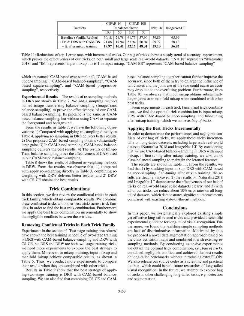
Figure 1: Overview of our proposed CAM-based sampling.For each image sampled by re-sampling, CAM is firstly gen-erated based on feature maps and FC weights of ground truthlabel c. We separate the foreground and background based onthe average of its CAM values, and subsequently we trans-form foreground while keeping background unchanged to getthe generated informative sampled dataset.

Experimental Results Experiments of mixup methods areshown in Table 5. Especially, we do not try all possible valuesof hyper-parameter α for the Beta distribution, which is notthe main purpose of our work. We can discover from Table 5that 1) both input mixup and manifold mixup deliver betterresults over baseline, and 2) when α is 1 and mixing uplocation is set to the pooling layer, input mixup and manifoldmixup achieve comparable results, which need to conductmore experiments with other tricks.

The results of fine-tuning after mixup training are shownin Table 6. We can find that fine-tuning after input mixuptraining can obtain further improvements, but fine-tuningafter manifold mixup gets worse results.

Two-Stage Training ProceduresTwo-stage training consists of imbalanced training and bal-anced fine-tuning. In this section, we focus on exploringdifferent methods of balanced fine-tuning. We firstly describeexisting fine-tuning methods and then present our CAM-based sampling approach.

Balanced Fine-Tuning after Imbalanced TrainingCNNs trained on imbalanced datasets without any re-

3451

Firststage

Second stageof DRS

CIFAR-10-LT CIFAR-100-LTImbalance factor

100 50 100 50

CE

Baselinewithout re-sampling

30.18 24.78 61.73 57.90

Randomunder-sampling

28.18 21.33 60.21 55.97

Randomover-sampling

28.88 21.52 59.76 55.90

Class-balancedsampling

29.04 21.34 59.56 55.67

Square-rootsampling

31.31 22.21 61.02 57.05

P-Bsampling

33.48 24.58 61.35 56.93

CAM-basedunder-sampling

24.98 19.15 58.99 54.17

CAM-basedover-sampling

24.87 18.82 58.45 54.36

CAM-basedbalance-sampling

24.63 18.60 58.27 54.05

CAM-basedsquare-sampling

28.14 20.69 60.07 55.61

CAM-basedprogressive-sampling

27.39 19.46 59.67 55.28

ImageTransbalance-sampling

28.10 21.60 59.28 55.05

Table 7: Top-1 error rates of different re-sampling methodsused in DRS. The proposed CAM-based sampling deliversbetter results. In particular, CAM-based balance-samplingobtains the best results. “P-B” represents “Progressively-balanced”.

Firststage

Second stageof DRW

CIFAR-10-LT CIFAR-100-LTImbalance factor

100 50 100 50

CE

CE 30.18 24.78 61.73 57.90Focal loss 29.71 23.77 61.74 57.32CB Focal 25.62 21.25 61.99 55.54

CS CE 25.31 20.81 58.92 54.57

Table 8: Top-1 error rates of different re-weighting methodsused in DRW. CS CE obtains the best results in DRW trainingschedule.

weighting or re-sampling method learn good featurerepresentations but suffer poor recognition accuracyon under-represented tail categories. Cui et al. (2018)fine-tune these networks on balanced subsets to make thelearned features from imbalanced datasets be transferredand re-balanced among all categories. These fine-tuningmethods (Cao et al. 2019) can be divided into two sections:deferred re-balancing by re-sampling (DRS) and byre-weighting (DRW).• DRS uses the vanilla training schedule firstly, and then

applies re-sampling for balanced fine-tuning. In order to geta balanced subset for fine-tuning, re-sampling methods in-

Firststage

Secondstage

CIFAR-10-LT CIFAR-100-LTImbalance factor

100 50 100 50

CE

CE 30.18 24.78 61.73 57.90CS CE 25.31 20.81 58.92 54.57

CAM-BS 24.63 18.60 58.27 54.05CS CE + CAM-BS 24.82 18.96 58.36 54.09

Table 9: Top-1 error rates of different strategies to apply DRWand DRS. Applying DRS (CAM-based balance-sampling)only shows the best result. “CAM-BS” represents “CAM-based balance-sampling”.

Trainingscheduler

Mixuptraining

CIFAR-10-LT CIFAR-100-LTImbalance factor

100 50 100 50DRS withCAM-BS

Manifold mixup 22.65 19.17 57.20 56.94Input mixup 21.88 17.94 53.94 50.04

Table 10: Top-1 error rates of combining mixup methodswith other best tricks. We can easily find that input mixupobtains larger gains over manifold mixup. “CAM-BS” repre-sents “CAM-based balance-sampling”. In mixup, α is 1 andmainifold mixup’s location is set to the pooling layer.

troduced in the section of “Re-sampling methods” will beapplied. Furthermore, we propose a sample yet effective gen-erative sampling method termed “CAM-based sampling”.• DRW uses the vanilla training schedule in the first stage,

and then applies re-weighting methods in the second stage.Re-weighting methods introduced in the section of “Re-weighting methods” will be applied in the second stage.

The Proposed CAM-Based Sampling for DRS Existingre-sampling methods used in DRS only replicate or removerandomly selected samples from the original dataset to gener-ate balanced subsets, which deliver limited improvements dur-ing balanced fine-tuning. In order to generate discriminativeinformation, inspired by class activation maps (CAM) (Zhouet al. 2016), we propose CAM-based sampling, which showsa significant accuracy improvement over existing methodswith a marginal extra cost.

As illustrated in Figure 1, we firstly apply re-sampling toget balanced sampled images. For each sampled image, weuse the parameterized model trained in the first training stageto generate CAM based on its ground truth label and corre-sponding fully-connected layer’s weights. The foregroundand background are separated based on the average valueof its CAM, where the foreground contains pixels largerthan the average and the background contains the rest (Weiet al. 2017). Finally, we apply transformations to the fore-ground while keeping the background unchanged. The trans-formation (implemented by Huawei MindSpore) includeshorizontal flipping, translation, rotating and scaling, and werandomly choose only one transformation for each image.

In concretely, we combine CAM with random over-sampling, random under-sampling, class-balanced sampling,square-root sampling, and progressively-balanced sampling,

3452

DatasetsCIFAR-10 CIFAR-100

iNat 18 ImageNet-LTImbalance factor100 50 100 50

Baseline (Vanilla ResNet) 30.18 24.78 61.73 57.90 39.89 65.99+ IM & DRS with CAM-BS 21.88 17.94 53.94 50.04 29.72 58.13

+ ft. after mixup training 19.97 16.41 52.17 48.31 29.13 56.87

Table 11: Reductions of top-1 error rates with incremental tricks. Our bag of tricks shows a steady trend of accuracy improvement,which proves the effectiveness of our tricks on both small and large scale real-world datasets. “iNat 18” represents “iNaturalist2018” and “IM” represents “input mixup”. α is 1 in input mixup. “CAM-BS” represents “CAM-based balance-sampling”

which are named “CAM-based over-sampling”, “CAM-basedunder-sampling”, “CAM-based balance-sampling”, “CAM-based square-sampling”, and “CAM-based progressive-sampling”, respectively.

Experimental Results The results of re-sampling methodsin DRS are shown in Table 7. We add a sampling methodnamed image transferring balance-sampling (ImageTransbalance-sampling) to prove the effectiveness of our CAM-based balance-sampling. Its pipeline is the same as CAM-based balance-sampling, but without using CAM to separatethe foreground and background.

From the results in Table 7, we have the following obser-vations: 1) Compared with applying re-sampling directly inTable 4, applying re-sampling in DRS delivers better results.2) Our proposed CAM-based sampling obtains substantiallylarge gains. 3) In CAM-based sampling, CAM-based balance-sampling delivers the best results. 4) The results of Image-Trans balance-sampling prove the effectiveness of CAM usedin our CAM-based balance-sampling.

Table 8 shows the results of different re-weighting methodsin DRW. From the results, we observe that: 1) comparedwith apply re-weighting directly in Table 3, combining re-weighting with DRW delivers better results, and 2) DRWwith CS CE obtains the best results.

Trick CombinationsIn this section, we first review the conflictual tricks in eachtrick family, which obtain comparable results. We combinethese conflictual tricks with other best tricks across trick fam-ilies, in order to find the best trick combination. Furthermore,we apply the best trick combination incrementally to showthe negligible conflicts between these tricks.

Removing Conflictual Tricks in Each Trick FamilyExperiments in the section of “Two stage training procedures”have shown the best training schedule of two-stage trainingis DRS with CAM-based balance-sampling and DRW withCS CE, but DRS and DRW are both two-stage training tricks,we need more experiments to explore the best strategy toapply them. Moreover, in mixup training, input mixup andmanifold mixup achieve comparable results, as shown inTable 5. Thus, we conduct more experiments to comparetheir results when they are combined with other tricks.

Results in Table 9 show that the best strategy of apply-ing two-stage training is DRS with CAM-based balance-sampling. We can also find that combining CS CE and CAM-

based balance-sampling together cannot further improve theaccuracy, since both of them try to enlarge the influence oftail classes and the joint use of the two could cause an accu-racy drop due to the overfitting problem. Furthermore, fromTable 10, we observe that input mixup obtains substantiallylarger gains over manifold mixup when combined with otherbest tricks.

From experiments in each trick family and trick combina-tions, we find the optimal trick combination is input mixup,DRS with CAM-based balance-sampling, and fine-tuningafter mixup training, which we name as bag of tricks.

Applying the Best Tricks IncrementallyIn order to demonstrate the performances and negligible con-flicts of our bag of tricks, we apply these tricks incremen-tally on long-tailed datasets, including large scale real-worlddatasets iNaturalist 2018 and ImageNet-LT. By consideringthat we use CAM-based balance-sampling in DRS with inputmixup, in fine-tuning after mixup training, we also adoptclass-balanced sampling to maintain the learned features.

The results are shown in Table 11. From the results, wefind that 1) by stacking input mixup, DRS with CAM-basedbalance-sampling, fine-tuning after mixup training, the re-sults are steadily improved, 2) the results on iNaturalist 2018and ImageNet-LT demonstrate the effectiveness of our bag oftricks on real-world large scale datasets clearly, and 3) withall of our tricks, we reduce about 10% error rates on all long-tailed datasets, which demonstrates significant improvementscompared with existing state-of-the-art methods.

ConclusionsIn this paper, we systematically explored existing simpleyet effective long-tail related tricks and provided a scientificexperimental guideline for long-tailed visual recognition. Fur-thermore, we found that existing simple sampling methodsare lack of discriminative information. Motivated by this,we proposed a novel data augmentation approach based onthe class activation maps and combined it with existing re-sampling methods. By conducting extensive experiments,we obtain the optimal trick combination, i.e., bag of tricks,contained negligible conflicts and achieved the best resultson long-tailed benchmarks without introducing extra FLOPs.We also release our source codes as a scientific and practicaltoolbox, which could benefit future researches of long-tailedvisual recognition. In the future, we attempt to explore bagof tricks in other challenging long-tailed tasks, e.g., detectionand segmentation.

3453

ReferencesBuda, M.; Maki, A.; and Mazurowski, M. A. 2018. A system-atic study of the class imbalance problem in convolutionalneural networks. Neural Networks 106: 249–259.

Cao, K.; Wei, C.; Gaidon, A.; Arechiga, N.; and Ma, T. 2019.Learning imbalanced datasets with label-distribution-awaremargin loss. In NeurIPS 32, 1565–1576.

Chawla, N. V.; Bowyer, K. W.; Hall, L. O.; and Kegelmeyer,W. P. 2002. SMOTE: Synthetic minority over-sampling tech-nique. Journal of Artificial Intelligence Research 16: 321–357.

Chu, P.; Bian, X.; Liu, S.; and Ling, H. 2020. Feature spaceaugmentation for long-tailed data. In ECCV.

Cui, Y.; Jia, M.; Lin, T.-Y.; Song, Y.; and Belongie, S. 2019.Class-balanced loss based on effective number of samples.In CVPR, 9268–9277.

Cui, Y.; Song, Y.; Sun, C.; Howard, A.; and Belongie, S. 2018.Large scale fine-grained categorization and domain-specifictransfer learning. In CVPR, 4109–4118.

Deng, J.; Dong, W.; Socher, R.; Li, L.-J.; Li, K.; and Fei-Fei, L. 2009. ImageNet: A large-scale hierarchical imagedatabase. In CVPR, 248–255.

Drummond, C.; and Holte, R. C. 2003. C4.5, class imbal-ance, and cost sensitivity: Why under-sampling beats over-sampling. In Workshop on learning from imbalanced datasetsII, volume 11, 1–8.

Goyal, P.; Dollar, P.; Girshick, R.; Noordhuis, P.; Wesolowski,L.; Kyrola, A.; Tulloch, A.; Jia, Y.; and He, K. 2017. Accurate,large minibatch SGD: Training ImageNet in 1 hour. arXivpreprint arXiv:1706.02677 .

Gupta, A.; Dollar, P.; and Girshick, R. 2019. LVIS: A datasetfor large vocabulary instance segmentation. In CVPR, 5356–5364.

Han, H.; Wang, W.-Y.; and Mao, B.-H. 2005. Borderline-SMOTE: A new over-sampling method in imbalanced datasets learning. In International Conference on IntelligentComputing, 878–887.

He, K.; Zhang, X.; Ren, S.; and Sun, J. 2015. Delving deepinto rectifiers: Surpassing human-level performance on ima-genet classification. In ICCV, 1026–1034.

He, K.; Zhang, X.; Ren, S.; and Sun, J. 2016. Deep residuallearning for image recognition. In CVPR, 770–778.

He, T.; Zhang, Z.; Zhang, H.; Zhang, Z.; Xie, J.; and Li, M.2019a. Bag of tricks for image classification with convolu-tional neural networks. In CVPR, 558–567.

He, Z.; Xie, L.; Chen, X.; Zhang, Y.; Wang, Y.; and Tian, Q.2019b. Data augmentation revisited: Rethinking the distribu-tion gap between clean and augmented data. arXiv preprintarXiv:1909.09148 .

Jamal, M. A.; Brown, M.; Yang, M.-H.; Wang, L.; and Gong,B. 2020. Rethinking class-balanced methods for long-tailedvisual recognition from a domain adaptation perspective. InCVPR, 7610–7619.

Japkowicz, N.; and Stephen, S. 2002. The class imbalanceproblem: A systematic study. Intelligent Data Analysis 6(5):429–449.Kang, B.; Xie, S.; Rohrbach, M.; Yan, Z.; Gordo, A.; Feng,J.; and Kalantidis, Y. 2020. Decoupling representation andclassifier for long-tailed recognition. In ICLR, 1–16.Krizhevsky, A.; and Hinton, G. 2009. Learning multiple lay-ers of features from tiny images. Technical report, Universityof Toronto.Lin, T.-Y.; Goyal, P.; Girshick, R.; He, K.; and Dollar, P. 2017.Focal loss for dense object detection. In ICCV, 2980–2988.Lin, T.-Y.; Maire, M.; Belongie, S.; Hays, J.; Perona, P.;Ramanan, D.; Dollar, P.; and Zitnick, C. L. 2014. MicrosoftCOCO: Common objects in context. In ECCV, volume 8693of LNCS, 740–755. Springer.Liu, Z.; Miao, Z.; Zhan, X.; Wang, J.; Gong, B.; and Yu, S. X.2019. Large-scale long-tailed recognition in an open world.In CVPR, 2537–2546.Mikolov, T.; Sutskever, I.; Chen, K.; Corrado, G. S.; andDean, J. 2013. Distributed representations of words andphrases and their compositionality. In NIPS 26, 3111–3119.More, A. 2016. Survey of resampling techniques for improv-ing classification performance in unbalanced datasets. arXivpreprint arXiv:1608.06048 .Ouyang, W.; Wang, X.; Zhang, C.; and Yang, X. 2016. Fac-tors in finetuning deep model for object detection with long-tail distribution. In CVPR, 864–873.Peng, M.; Zhang, Q.; Xing, X.; Gui, T.; Huang, X.; Jiang,Y.-G.; Ding, K.; and Chen, Z. 2019. Trainable undersamplingfor class-imbalance learning. In AAAI, 4707–4714.Perez-Ortiz, M.; Tino, P.; Mantiuk, R.; and Hervas-Martınez,C. 2019. Exploiting synthetically generated data with semi-supervised learning for small and imbalanced datasets. InAAAI, 4715–4722.Sarafianos, N.; Xu, X.; and Kakadiaris, I. A. 2018. Deep im-balanced attribute classification using visual attention aggre-gation. In ECCV, volume 11215 of LNCS, 708–725. Springer.Shen, L.; Lin, Z.; and Huang, Q. 2018. Relay backpropaga-tion for effective learning of deep convolutional neural net-works. In ECCV, volume 9911 of LNCS, 185–201. Springer.Van Horn, G.; Mac Aodha, O.; Song, Y.; Cui, Y.; Sun, C.;Shepard, A.; Adam, H.; Perona, P.; and Belongie, S. 2018.The iNaturalist species classification and detection dataset.In CVPR, 8769–8778.Verma, V.; Lamb, A.; Beckham, C.; Najafi, A.; Mitliagkas, I.;Lopez-Paz, D.; and Bengio, Y. 2019. Manifold Mixup: Betterrepresentations by interpolating hidden states. In ICML,6438–6447.Wang, H.; Wang, Y.; Zhou, Z.; Ji, X.; Gong, D.; Zhou, J.; Li,Z.; and Liu, W. 2018. CosFace: Large margin cosine loss fordeep face recognition. In CVPR, 5265–5274.Wang, T.; Li, Y.; Kang, B.; Li, J.; Liew, J. H.; Tang, S.; Hoi,S.; and Feng, J. 2019. Classification calibration for long-tailinstance segmentation. arXiv preprint arXiv:1910.13081 .

3454

Wang, Y.-X.; Ramanan, D.; and Hebert, M. 2017. Learningto model the tail. In NIPS 30, 7029–7039.Wei, X.-S.; Luo, J.-H.; Wu, J.; and Zhou, Z.-H. 2017. Se-lective convolutional descriptor aggregation for fine-grainedimage retrieval. IEEE Transactions on Image Processing26(6): 2868–2881.Wei, X.-S.; Wu, J.; and Cui, Q. 2019. Deep learningfor fine-grained image analysis: A survey. arXiv preprintarXiv:1907.03069 .Xiang, L.; Ding, G.; and Han, J. 2020. Learning from multi-ple experts: Self-paced knowledge distillation for long-tailedclassification. In ECCV.Yan, Y.; Tan, M.; Xu, Y.; Cao, J.; Ng, M.; Min, H.; and Wu,Q. 2019. Oversampling for imbalanced data via optimaltransport. In AAAI, 5605–5612.Yu, Q.; and Lam, W. 2019. Data augmentation based onadversarial autoencoder handling imbalance for learning torank. In AAAI, 411–418.Zhang, H.; Cisse, M.; Dauphin, Y. N.; and Lopez-Paz, D.2018. mixup: Beyond empirical risk minimization. In ICLR,1–13.Zhang, X.; Fang, Z.; Wen, Y.; Li, Z.; and Qiao, Y. 2017.Range loss for deep face recognition with long-tailed trainingdata. In ICCV, 5409–5418.Zhang, Z.; He, T.; Zhang, H.; Zhang, Z.; Xie, J.; and Li, M.2019. Bag of freebies for training object detection neuralnetworks. arXiv preprint arXiv:1902.04103 .Zhou, B.; Cui, Q.; Wei, X.-S.; and Chen, Z.-M. 2020. BBN:Bilateral-branch network with cumulative learning for long-tailed visual recognition. In CVPR, 9719–9728.Zhou, B.; Khosla, A.; Lapedriza, A.; Oliva, A.; and Torralba,A. 2016. Learning deep features for discriminative localiza-tion. In CVPR, 2921–2929.Zhou, B.; Lapedriza, A.; Khosla, A.; Oliva, A.; and Torralba,A. 2017. Places: A 10 million image database for scenerecognition. IEEE Transactions on Pattern Analysis andMachine Intelligence 40(6): 1452–1464.

3455