Bacterial Total Maximum Daily Load Task Force Reporttwri.tamu.edu/docs/bacteria-tmdl/tsswcb comments on …  · Web viewTask Force Report. First Draft. ... measuring the diameter

Bacterial Total Maximum Daily Load

Task Force Report

First Draft

October 30, 2006

Table of Contents

Introduction 1

Bacteria Fate and Transport Models 2

Bacteria Source Tracking 9

Recommended Decision-Making Process for Texas 16TMDL and Implementation Plan DevelopmentResearch and Development Needs

Research and Development Needs 17

References 18

Appendix 1: EPA Bacteria TMDL Guidelines 20

Appendix 2: State Approaches to Bacteria TMDL 29Development

Appendix 3: Models Used in Bacteria ProjectsSource 39

Tracking as Described in EPA Publications

Appendix 4: Bacteria TMDL Task Force Personnel 44

Appendix 5: Comments from Expert Advisory Group 46

Introduction

On September 279, 2006, the Texas Commission on Environmental Quality (TCEQ) and

the Texas State Soil and Water Conservation Board (TSSWCB) established a joint

technical Task Force on Bacteria TMDLs. The Task Force was charged with:

reviewing U.S. Environmental Protection Agency (EPA) Total Maximum Daily

Load (TMDL) guidelines and approaches taken by selected states to TMDL and

implementation plan (I-Plan) development

evaluating scientific tools, including bacteria fate and transport modeling and

bacterial source tracking (BST)

suggesting alternative approaches using bacteria modeling and BSTsource

tracking for TMDL and I-Planimplementation plan and watershed protection plan

development, emphasizing scientific quality, timeliness and cost effectiveness

identifying gaps in our understanding of bBacteria fate and transport requiring

additional research and tool development

Task Force members are Drs. Allan Jones, Task Force Cchair, Texas Water Resources

Institute; George Di Giovanni, Texas Agricultural Experiment Station–El Paso; Larry

Hauck, Texas Institute for Applied Environmental Research; Joanna Mott, Texas A&M

University–Corpus Christi; Hanadi Rifai, University of Houston; Raghavan Srinivasan,

Texas A&M University; and George Ward, The University of Texas at Austin.

Approximately 40 Expert Advisors (Appendix 4) with expertise on bacteria related issues

have also provided significant input to the Task Force during the process. Additionally,

local, state and federal agencies with jurisdictions impacting bacteria and water quality

offered guidance to the Task Force.

Recommendations from the Task Force are intended to be used by the State of Texas,

specifically can be used by TSSWCB and TCEQ, to keep Texas as a national leader in

water quality protection.

1

Bacteria Fate and Transport Models

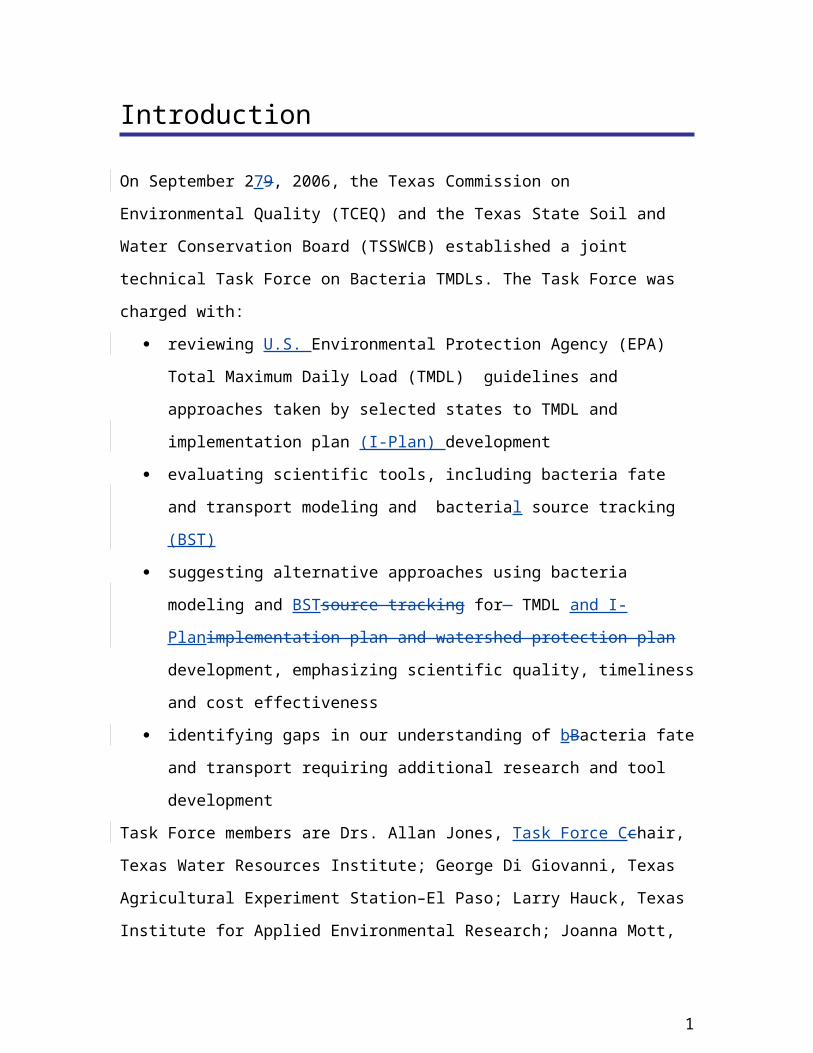
This section, coordinated by Drs. Hanadi Rifai and Raghavan Srinivasan, describes the

strengths and weaknesses of several bacterial fate and transport models that have been

used in Texas TMDL and/or implementation plan development. A more complete list of

modeling tools taken from EPA publication is in Appendix 3.

Bacterial pollution in surface water bodies is a complex phenomenon to model because of

the numerous sources of pathogens in a given watershed and the various fate and

transport processes that control their behavior and distribution in water systems. Bacterial

indicators such as E. coli , Enterococcus spp., and fecal coliform originate from human

and non-human sources and they are released into water bodies via end-of-pipe sources

(such as wastewater treatment plant effluent and runoff from drainage networks) as well

as dispersed (or non-point) sources (such as direct deposition from birds and re-

suspension from sediment). Bacteria are present in water and sediment, and experience

re-growth and death within a water body. Furthermore, bacteria loads into a stream vary

spatially and temporallyover time because of the variability of flow within the stream

network and because of the different loads coming from the various sources at different

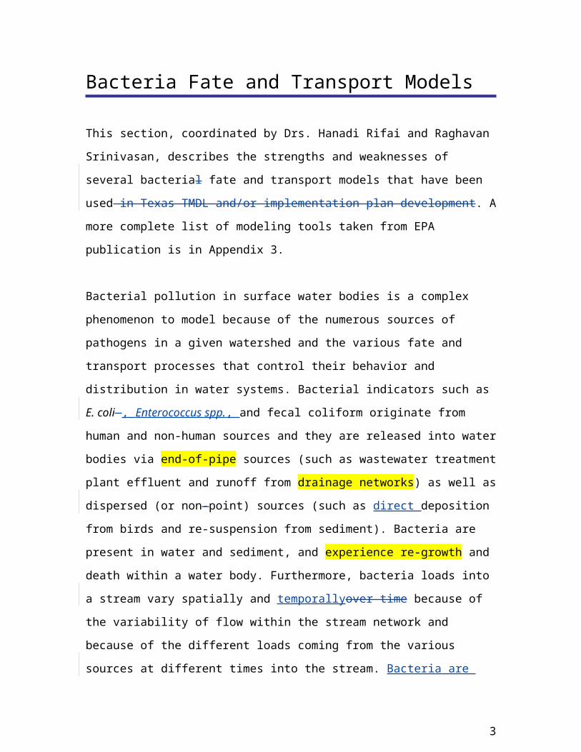
times into the stream. Bacteria are living organisms and do not behave like chemical

water quality parameters. These factors and considerations motivate the need desire for

using models in the bacteria TMDL process. However, selecting an appropriate model for

bacteria TMDLs is a challenging problem in and of itself, due to the numerous water

quality models that are available. Thus, establishing the goal of the modeling within the

context of a TMDL is a very important and critical step that needs to be undertaken early

on in the process.

Since bacteria TMDLs estimate the maximum bacteria load that a waterbody can receive

and still meet water quality standards, TMDL development involves estimating both

existing and allowable loads, as well as the reductions that would be required to meet

standards. TMDL implementation, on the other hand, involves designing bacteria

reduction strategies and examining their effects on water quality. These differing goals

2

between TMDL development and implementation may necessitate the use of different

bacteria models with different levels of sophistication.

The two basic modeling strategies that have been used for developing and implementing

TMDLs involve: (1) the use of statistical models or mass balance models that rely on

available flow and water quality data, and (2) the use of in-stream water quality computer

models. The most common models within the two strategies that have been used for

bacteria TMDLs are described below.

Statistical and Mass Balance Bacteria Models

The most common of the statistical models used in bacteria TMDLs has been the Load

Duration Curve. Mass balance methods, on the other hand, while commonly used, are not

uniform in their approach and tend to be watershed specific.

Load Duration Curves (LDC)

This method is used in TMDL development for estimating existing and allowable loads,

and the reductions required to meet the water quality standard. This method can also only

be used in a generic sense to allocate sources to end-of-pipe and non-point sources. The

LDC method, however, is not as well suited for TMDL implementation and development

of strategies for load reductions within the watershed because it cannot be used to

estimate loads from specific sources within the watershed.

Briefly, the LDC method involves developing a flow duration curve or a representation of

the percentage of days in a year when a given flow occurs. The allowable bacteria load

curve is calculated using this flow duration curve by multiplying the flow values by the

applicable bacterial standard. The observed bacteria loads in the water body are plotted

on the developed curve and the points that fall above the allowable bacteria loads curve

indicate exceedances while the points that fall below the curve indicate acceptable loads.

3

The advantage of this method is its simplicity, and the need for minimal data

requirements. Existing loading, and load reductions required to meet the TMDL water

quality target, can be calculated under different flow conditions. The main disadvantage

as mentioned previously is the method does not allow estimating loads from specific

sources within the watershed, and does not account for spatial and temporal variations in

source or in-stream loads.

Mass Balance Method

The method, as the name implies, involves undertaking a mass balance between source

loads entering the water body and the bacteria load within the stream. Sources are

typically inventoried, quantified and compared to existing and allowable in-stream loads

at specified points within the stream (typically, where the TMDL is sought) for different

flow conditions. Mass balance methods require more data than the LDC method, but are

more amenable for use in TMDL implementation. These methods have typically been

developed using spreadsheets. The main advantages of the mass balance method are that

they can be used for tidal and non-tidal water bodies, for TMDL development and

implementation, and more importantly for watersheds where the distinction between end-

of-pipe and non-point sources is not apparent at the different flow levels (in other words,

both categories of sources come into play at low flow and high flow). The main

disadvantage is that the mass balance method, similar to the LDC method, is static and

does not allow for temporal variations in loading. The mass balance method, however,

does account for spatial variations since it estimates the various sources within the

watershed.

In Texas, one of the more recent mass balance applications is described in Petersen

(2006). They developed a Bacteria Load Estimator Spreadsheet Tool (BLEST) that

calculates bacteria loads from all sources and land -uses on a subwatershed basis for

Buffalo and White Oak Bayous. The loads are accumulated by segment and calculated

for low flow, median flow and high flow conditions in a stream. Sources include

wastewater treatment plants, septic tanks, runoff, overflows and bypasses, sewer leaks

and spills, in-stream sediment and wildlife and domesticated animals in watersheds. The

4

BLEST was used to calculate existing loads and allowable loads and to estimate the load

reductions that would be required to meet the standard.

5

In-Stream Bacteria Models

These models can be used both for TMDL development and implementation and for

evaluating spatial and temporal variation of bacterial loading within a watershed. These

models, however, suffer from their extensive data requirements, their level of

sophistication that necessitates a significant investment in resources, and their complex

nature that makes them less amenable for use by the stakeholders. In general, in-stream

water quality models are steady-state or transient and they are typically hydrogically

driven (via rainfall) or hydrodynamically driven (via velocities in the water body). A

steady-state model does not allow for variations over time, and, in essence, shows a

“snapshot” of water quality in a stream. A dynamic or transient model, on the other hand,

allows for changes over time and can be used to estimate bacteria loads and

concentrations at different points in time anywhere in the stream.

Ward and Benaman (1999) identified a number of models as being appropriate for use in

Texas TMDLs. Their list includes: ANSWERS, CE-QUAL-W2, DYNHYD, EFDC,

GLEAMS, HSPF, POM, PRMS, QUALTX, SWAT, SWMM, TxBLEND and WASP.

Their assessment categorized these models based on the watercourse type and the scale of

resolution for time. So for example, HSPF, SWAT, PRSM, SWMM and ANSWERS

were characterized as watershed type models that can be used for “slow time variation”

and “continuous time variation,” and all but SWAT can be used to model the time scale

for a single storm event.

Of the above list of models identified by Ward and Benaman (1999) for use in Texas

TMDLs, the most commonly used for bacteria include: HSPF, SWAT, SWMM, and

WASP, with HSPF being the most popular of the four. These models have many

similarities and differences. They all share the characteristics of being data intensive and

difficult to apply, i.e., all four models require many input variables, a substantial

investment in set-up, calibration and validation time, and have a steep learning curve. The

differences between the four models are discussed below.

6

HSPF (Hydrological Simulation Program – FORTRANDynamic Rainfall-driven

Model)

HSPF (Hydrological Simulation Program – FORTRAN) is distributed by EPA’s Center

for Exposure Assessment Modeling. The model is data intensive and has been commonly

used for bacteria TMDLs in Texas and other states. The required data include land use,

watershed and subwatershed boundaries, location and data for rainfall gages and surface

water quality monitoring stationsgages, detailed descriptions of stream geometry and

capacity, detailed information about sources within the watershed, sedimentation and re-

suspension characteristics, and bacteria die-off rates, to name a few. Development of an

HSPF model for a given watershed is both complex and time consuming and involves a

calibration and validation step. The advantage of HSPF is it can be used for any type of

watershed regardless of the land use, and it relies on hydrologic and hydraulic models as

well as GIS data layers for its input. HSPF allows for a detailed spatial resolution within

the watershed and allows for estimation of bacterial loads from runoff and from sediment

wash-off from the land surface as well as re-suspension from the bed stream and from

direct deposition sources. Additionally, HSPF simulates in-stream water quality. The

disadvantages include the inherent difficulty in its application, its poor documentation

and inadequate simulation of bacteria fate and transport processes (for example, transport

of bacteria associated with sediment, sedimentation and re-suspension, re-growth and die-

off processes are simplified and end up being treated as calibration variables). HSPF

additionally was not designed to model reservoirs.

SWAT (Soil and Water Assessment Tool)

The SWAT model is a continuation of nearly 30 years of modeling efforts conducted by

the United States Department of Agriculture (USDA) Agricultural Research Service

(ARS). SWAT has gained international acceptance as a robust interdisciplinary

watershed modeling tool as evidenced by international SWAT conferences, SWAT-

related papers presented at numerous other scientific meetings, and dozens of articles

published in peer-reviewed journals. The model has also been adopted as part of the EPA

Better Assessment Science Integrating Point & Nonpoint Sources (BASINS) software

7

package and is being used by many federal and state agencies, including the USDA

within the Conservation Effects Assessment Project (CEAP). Reviews of SWAT

applications and/or components have been previously reported, sometimes in conjunction

with comparisons with other models (e.g., Arnold and Fohrer, 2005; Borah and Bera,

2003; Borah and Bera, 2004; Steinhardt and Volk, 2003). (Gassman, et.al 2005).

This model, developed as an improvement over SWRRB, was primarily developed to

estimate loads from rural and mainly agricultural watersheds; however, the capability for

including impervious cover was accomplished by adding urban build up/wash off

equations from SWMM. A microbial sub-model was incorporated to SWAT for use at the

watershed or river basin levels. The microbial sub-model simulates (1) functional

relationships for both the die-off and re-growth rates and (2) release and transport of

pathogenic organisms from various sources that have distinctly different biological and

physical characteristics. SWAT has been used in Virginia and North Carolina for

bacterial TMDL development.

SWMM (Storm Water Management Model)

This model was developed primarily for urban areas. SWMM simulates real storm events

based on meteorological data and watershed data, and that has been the most common

way for applying the model, although it can be used for continuous simulations. While

SWMM was developed with urban watersheds in mind, it can be used for other

watersheds. The biggest advantage of SWMM is in its ability to model the detailed urban

drainage infrastructure including drains, detention basins, sewers and related flow

controls. One of the key disadvantages of SWMM, however, is it does not simulate the

in-stream water quality or the quality within the receiving stream. This limitation can be

circumvented by linking it to WASP. Perhaps the best application for SWMM can be to

characterized as the bacterial pollution from the urban drainage infrastructure but this

somewhat limits the usefulness of SWMM within a bacterial TMDL context to

implementation rather than TMDL development.

8

WASP (Water-quality Analysis Simulation Program)

This model is also distributed by EPA’sthe Center for Exposure Assessment Modeling of

EPA. It is a well-established water quality model incorporating transport and reaction

kinetics water quality model like HSPF. Unlike HSPF, however, WASP is not rainfall-

driven, rather it is velocity-driven, thus it is usually coupled with a suitable hydro-

dynamic model such as DYNHYD that calculates the velocities. WASP is typically used

for main channels and for bays and estuaries and not for modeling watershed-scale

processes and sources of bacteria.

9

Bacterial Source Tracking

This section, coordinated by Drs. Joanna Mott and George Die Giovanni and Joanna

Mott, describes the strengths and weaknesses of several bBacterial sSource tTracking

(BST) tools that have been used in bacterial TMDL development in Texas.

The premise behind BST is that genetic and/or phenotypic tests can identify bacterial

strains that are host specific so that the original host animal and source of the fecal

contamination can be identified. Often Escherichia coli (E. coli) or Enterococcus spp. are

used as the bacteria targets in source tracking (for example, (Parveen, Portier et al. 1999;

Dombek, Johnson et al. 2000; Graves, Hagedorn et al. 2002; Griffith, Weisberg et al.

2003; Hartel, Summer et al. 2003; Kuntz, Hartel et al. 2003; Stoeckel, Mathes et al. 2004;

Scott, Jenkins et al. 2005)). While there has been some controversy concerning host

specificity and survival of E. coli in the environment (Gordon, Bauer et al. 2002), this

indicator organism has the advantage that it is known to correlate with the presence of

fecal contamination and is used for human health risk assessments. Bacterial source

tracking of E. coli, therefore, has the advantages of direct regulatory significance and

availability of standardized culturing techniques for water samples, such as EPA’s

Method 1603 (USEPA 2005).

There have been many different technical approaches to bacterial source tracking

(reviewed by Scott, Rose et al. 2002; Simpson, Santo Domingo et al. 2002; Meays,

Broersma et al. 2004), but there is currently no consensus on a single method for

field application. Genotypic tools appear to hold promise for BMST, providing the

most conclusive characterization and level of discrimination for isolates. Of the

molecular tools available, ribosomal ribonucleic acid (RNA) genetic fingerprinting

(ribotyping), repetitive element polymerase chain reaction (rep-PCR) and pulsed-

field gel electrophoresis (PFGE) are emerging as a few of the versatile and feasible

BMST techniques. Antibiotic resistance profiling, a phenotypic characterization

method, also has the potential to identify the human or animal origin of isolates, and

10

variations of this technique have been applied in several BMST studies. (See Table 1

below)

11

Technique Acronym Target organism(s)

Basis of characterizati

on

Previously Used in Texas

Used in

other states

Accuracy of source

identification

Size of library needed

for water isolate

IDs

Capital cost

Cost per sample

(reagents and

consumables only)

Ease of use

Hands on processing time for 32

isolates

Time required to complete

processing 32 isolates

Enterobacterial repetitive intergenic consensus sequence polymerase chain

reaction

ERIC-PCR

Escherichia coli

(E. coli) and Enterococcu

s spp.

DNA fingerprint

Yes(Di

Giovanni)Yes Moderate Moderat

e

$20,000($15,000

BioNumerics software, $5,000

equipment)

$8 Moderate 3 h 24 h**

Automated ribotyping

(RiboPrinting)†RP

E. coli and Enterococcu

s spp.

DNA fingerprint

Yes(Di

Giovanni)Yes Moderate Moderat

e

$115,000($100K

RiboPrinter, $15K BioNumerics

software)

$40 Easy 1 h 24 h

Pulsed field gel electrophoresis PFGE

E. coli and Enterococcu

s spp.

DNA fingerprint

Yes(Pillai and Lehman)

Yes High Large $30,000 $40 Difficult 10 h 5 days

Kirby-Bauer antibiotic resistance

analysis‡KB-ARA

E. coli and Enterococcu

s spp.

Phenotypic fingerprint

Yes(Mott) Yes Moderate* Moderat

e $35,000 $15 Easy 3 h 24 h**

Carbon source utilization CSU

E. coli and Enterococcu

s spp.

Phenotypic fingerprint

Yes(Mott) Yes Moderate Moderat

e $15,000 $10 Easy 4 h 24 h**

Bacteriodales polymerase chain

reaction

Bacterio-dales PCR

Bacteriodales species

Genetic marker

presence or absence

(not quantitative)

No Yes

Moderate to high for

only human,

ruminant, horse, and pig sources

Not applicabl

e $5,000 $8 Easy to

moderate 3 h 8 h**

Enterococcus faecium surface

protein polymerase chain reaction or

colony hyb.

E. faecium esp marker E. faecium

Genetic marker

presence or absence

(not quantitative)

No Yes High for only human

Not applicabl

e$8,000 $8 to $12 Easy to

moderate 3 to 6 h 8 to 24 h**

ERIC and RP 2-method composite ERIC-RP E. coli DNA

fingerprints

Yes(Di

Giovanni)No Moderate

to highModerat

e $120,000 $48 Moderate 4 h 24 h

ERIC and KB-ARA 2-method composite ERIC-ARA E. coli

DNA and phenotypic fingerprints

Yes(Di

Giovanni)No Moderate

to highModerat

e $55,000 $23 Moderate 6 h 24 h

KB-ARA and CSU 2-method composite ARA-CSU

E. coli and Enterococcu

s spp.

Phenotypic fingerprints

Yes(Mott) Yes Moderate

to highModerat

e $50,000 $23 Easy to moderate 7 h 24 h

Table 1. Relative comparison of several bacterial source tracking techniques

†A manual ribotyping version is also used by some investigators (e.g. Dr. M. Samadpour with University of Washington in Seattle), but no detailed information is available for comparison.‡A variation of this technique, called ARA, has been used extensively in Virginia for TMDLs. *This technique is better for distinguishing broader groups of pollution sources. For example, “wildlife” and “livestock” as opposed to “avian wildlife”, “non-avian wildlife”, “cattle”, etc.**With sufficient personnel, up to approximately 150 isolates can be analyzed in 24 h.

12

Each of these methods has its strengths and weaknesses, which are described below.

A disadvantage of all of the techniques is that reference libraries of genetic or phenotypic

fingerprints for E. coli isolated from known sources (e.g., domestic sewage, livestock and

wildlife) are needed to identify the sources of bacteria isolated from environmental water

samples. Thus, the development of an identification library can be a time consuming and

expensive component of a BST study.

ERIC-PCR

Enterobacterial repetitive intergenic consensus sequence polymerase chain reaction

(ERIC-PCR), a type of rep-PCR, has moderately high ability to resolve different closely

related bacterial strains. Consumable costs for ERIC-PCR are inexpensive and labor costs

for sample processing and data analyses are moderate. ERIC-PCR is a genetic

fingerprinting method used in previous BST studies as well as many microbial ecology

and epidemiological studies. ERIC elements are repeat DNA sequences found in varying

numbers and locations in the genomes of different bacteria such as E. coli. The PCR is

used to amplify the DNA regions between adjacent ERIC elements. This generates a

DNA banding pattern or fingerprint which looks similar to a barcode pattern. Different

strains of E. coli bacteria have different numbers and locations of ERIC elements in their

bacterial genomes, and therefore, have different ERIC-PCR fingerprints. ERIC-PCR was

chosen as the screening technique because of its moderate cost and moderately high

ability to resolve different strains of the same species of bacteria.

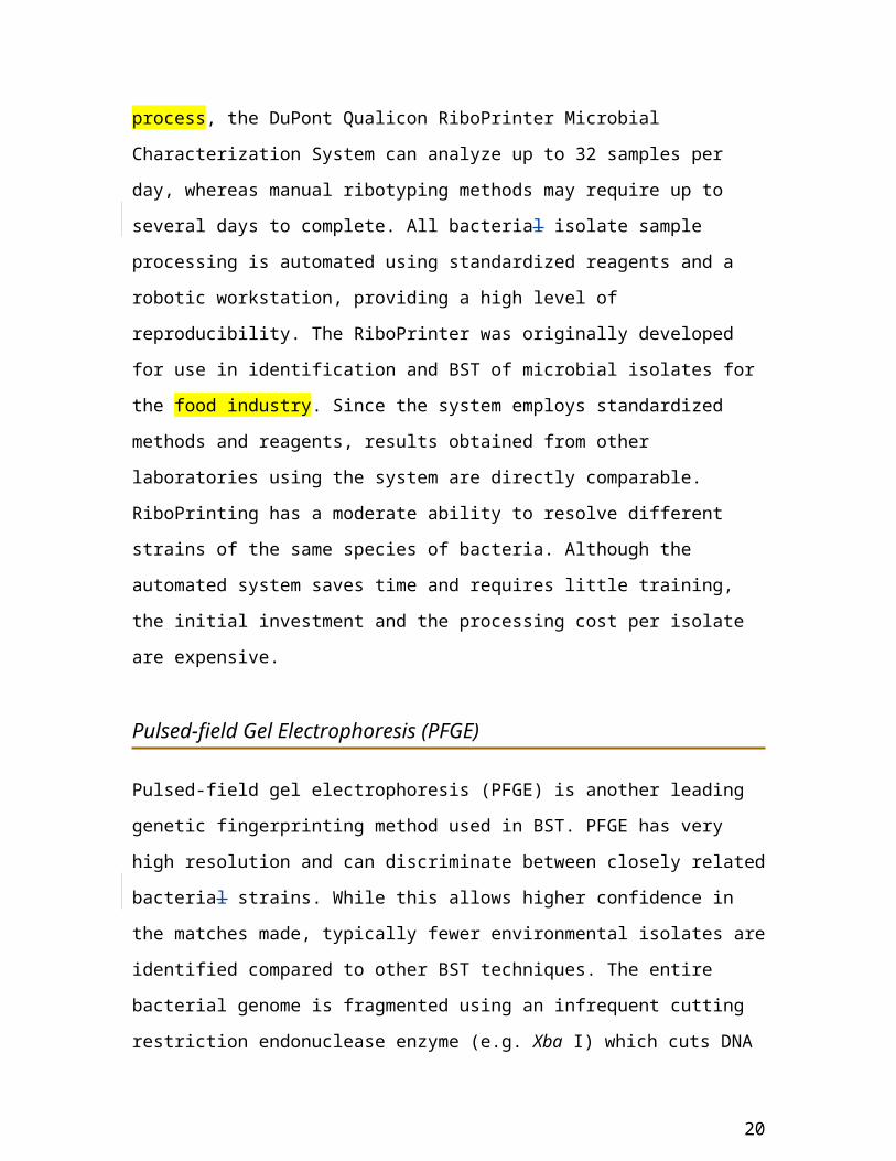
Ribotyping

Ribotyping is a genetic fingerprinting method used in previous BST studies as well as

many microbial ecology and epidemiological studies, although there is not a consensus as

to the best protocol. Ribotyping has a moderate ability to resolve different strains of the

same bacterial species. An automated ribotyping system is available, which saves labor

costs and requires little training, but the initial investment and the consumable cost per

isolate are expensive. In general, an endonuclease enzyme (Hind III) selectively cuts

13

E. coli DNA wherever it recognizes a specific DNA sequence. The resulting DNA

fragments are separated by size and probed for fragments containing particular conserved

ribosomal RNA gene sequences, which results in DNA banding patterns or fingerprints

that look similar to barcode patterns. Different strains of E. coli bacteria have differences

in their DNA sequences and different numbers and locations of enzyme cutting sites, and

therefore have different ribotyping fingerprints. By automating the process, the DuPont

Qualicon RiboPrinter Microbial Characterization System can analyze up to 32 samples

per day, whereas manual ribotyping methods may require up to several days to complete.

All bacterial isolate sample processing is automated using standardized reagents and a

robotic workstation, providing a high level of reproducibility. The RiboPrinter was

originally developed for use in identification and BST of microbial isolates for the food

industry. Since the system employs standardized methods and reagents, results obtained

from other laboratories using the system are directly comparable. RiboPrinting has a

moderate ability to resolve different strains of the same species of bacteria. Although the

automated system saves time and requires little training, the initial investment and the

processing cost per isolate are expensive.

Pulsed-field Gel Electrophoresis (PFGE)

Pulsed-field gel electrophoresis (PFGE) is another leading genetic fingerprinting method

used in BST. PFGE has very high resolution and can discriminate between closely related

bacterial strains. While this allows higher confidence in the matches made, typically

fewer environmental isolates are identified compared to other BST techniques. The entire

bacterial genome is fragmented using an infrequent cutting restriction endonuclease

enzyme (e.g. Xba I) which cuts DNA wherever it recognizes a specific rare sequence. All

the DNA fragments are separated by size and visualized resulting in a genetic fingerprint

that resembles a barcode. Different strains of E. coli bacteria have differences in their

DNA sequences and different numbers and locations of enzyme cutting sites and

therefore, have different PFGE fingerprints. PFGE is currently being used by the Centers

for Disease Control and Prevention (CDC) to track foodborne E. coli O157:H7 and

Salmonella isolates. CDC currently uses this standardized protocol as the basis of their

14

“PulseNet” outbreak surveillance network that allows public health laboratories

nationwide to quickly compare their PFGE fingerprints to the CDC central reference

library. Although it requires more training and cost, PFGE has very high resolution and

can discriminate between closely related strains. While this allows higher confidence in

the matches made, fewer species identifications can be made, and a very large (and

costly) library is needed for field application. In addition, some bacterial strains have

genomic DNA in configurations that do not permit effective restriction endonuclease

digestions.

Kirby-Bauer Antibiotic Resistance Analysis (KB-ARA)

The Kirby-Bauer antibiotic resistance analysis (KB-ARA) technique follows procedures

used in the clinical laboratory for evaluating the antibiotic resistance of bacterial isolates.

Of these four methods, a Antibiotic resistance analysis using the Kirby-Bauer method has

the lowest ability to discriminate closely related bacterial strains. It also has the lowest

initial and per sample cost and takes the least time and training, but the statistical analysis

of data can be complex and time-consuming.

Commonly, the disk diffusion method is used which involves measuring the diameter of

the zone of inhibition of bacterial growth around a filter disk impregnated with a specific

antibiotic. By comparison to resistant and susceptible control strains, the response of the

E. coli isolates can be determined. To further standardize and automate the assay, an

image analysis system is used to measure the zones of inhibition and provide electronic

archival of data. The KB-ARA profile for an isolate consists of the measurements of the

zones of inhibition in response to 20 antibiotics, each at a standard single concentration.

Of the methods mentioned, KB-ARA has the lowest ability to discriminate closely related

bacterial strains. However, it also has the lowest initial and per sample cost and takes the

least time and training, although the statistical analysis can be complex.

15

Recently, a BST project was completed for Lake Waco and Belton Lake in which E. coli

isolates were analyzed using RP, ERIC-PCR, PFGE and KB-ARA. BST analyses were

performed using the individual techniques, as well as composite data sets. The four-

method composite library generated the most desirable BST results in the study.

However, as few as two methods in combination may be useful based on congruence

measurements, library internal accuracy (i.e. rates of correct classification, RCCs), and

comparison of water isolate identifications. In particular, the combinations of ERIC-PCR

and RiboPrinting (ERIC-RP), or ERIC-PCR and Kirby-Bauer antibiotic resistance

analysis (ERIC-ARA) appeared promising. These two-method composite data sets were

found to have 90.7% and 87.2% congruence, respectively, to the four-method composite

data set. More importantly, based on the identification of water isolates, they identified

the same leading sources of fecal pollution as the four-method composite library. ERIC-

ARA has the lowest cost for consumables and has high sample throughput, but requires a

considerable amount of hands-on sample and data processing. Due to the high cost of

RiboPrinting consumables and instrumentation, ERIC-RP has a higher cost than ERIC-

ARA. However, ERIC-RP has the advantage of automated sample processing and data

preprocessing that the RiboPrinter system provides. Further research is needed to

determine if a regional library built from different projects using the same protocols may

be useful for the identification of water isolates from other watersheds.

Regulatory State agencies continue to have high hopes and expectations for BST in

aiding them to address water quality issues. Ideally, the regulatory state agencies would

prefer identification of pollution sources to the level of individual animal species.

Performing a three-way split of pollution sources into domestic sewage, livestock and

wildlife source classes would likely be more scientifically justified. The division of host

sources into the seven classes in this study was a compromise between the capabilities of

the BST techniques and their practical application. Since this study was initiated there

have been significant developments in library-independent BST methods, including

bacterial genetic markers specific to different animal sources and humans (for example,

(Bernhard and Field 2000; Dick, Bernhard et al. 2005; Scott, Jenkins et al. 2005;

Hamilton, Yan et al. 2006)). Library-independent methods are cost-effective, rapid and

16

potentially more specific than library-independent methods. Concerns with many of the

recently developed library-independent approaches include uncertainties regarding

geographical stability of markers and the difficulty of interpreting results in relation to

regulatory water quality standards and microbial risk, since some target microorganisms

are not regulated. More importantly, these library-independent methods can only detect a

limited range of pollution sources. For example, the Bacteriodales PCR (Field and

coworkers) can detect ruminants, humans, horses and pigs; but no further discrimination

is possible. For future studies, an assessment phase using a “toolbox” approach is

recommended. The assessment phase should include targeted monitoring of suspected

pollution sources, use of library-independent methods to identify the presence of

domestic sewage pollution, and screening of water isolates from the new watershed

against the previously developed Texas library to determine the need for collection of

local source samples and expansion of the library. Currently, we are cross-validating the

library generated in this study with a library generated for another Texas watershed in an

attempt to explore issues of geographical and temporal stability of BST libraries, refine

library isolate selection, and determine accuracy of water isolate identification.

17

Recommended Decision-Making Process forTexas TMDL and I-mplementation Plan Development

This section recommends a decision tree to be used in choosing appropriate bacterial

source tracking and bacterial fate and transport modeling approaches for Texas

conditions.

(A first draft of this section will be developed for Draft 2.)

18

Research and Development Needs

This section, coordinated by Drs. George Ward and Larry Hauck and George Ward,

describes research and development needed in the next three to five years to improve the

tools and methods available to TCEQ and TSSWCB for bacterial TMDL and I-

Pimplementation plan development.

(A first draft of this section will be developed for Draft 2.)

19

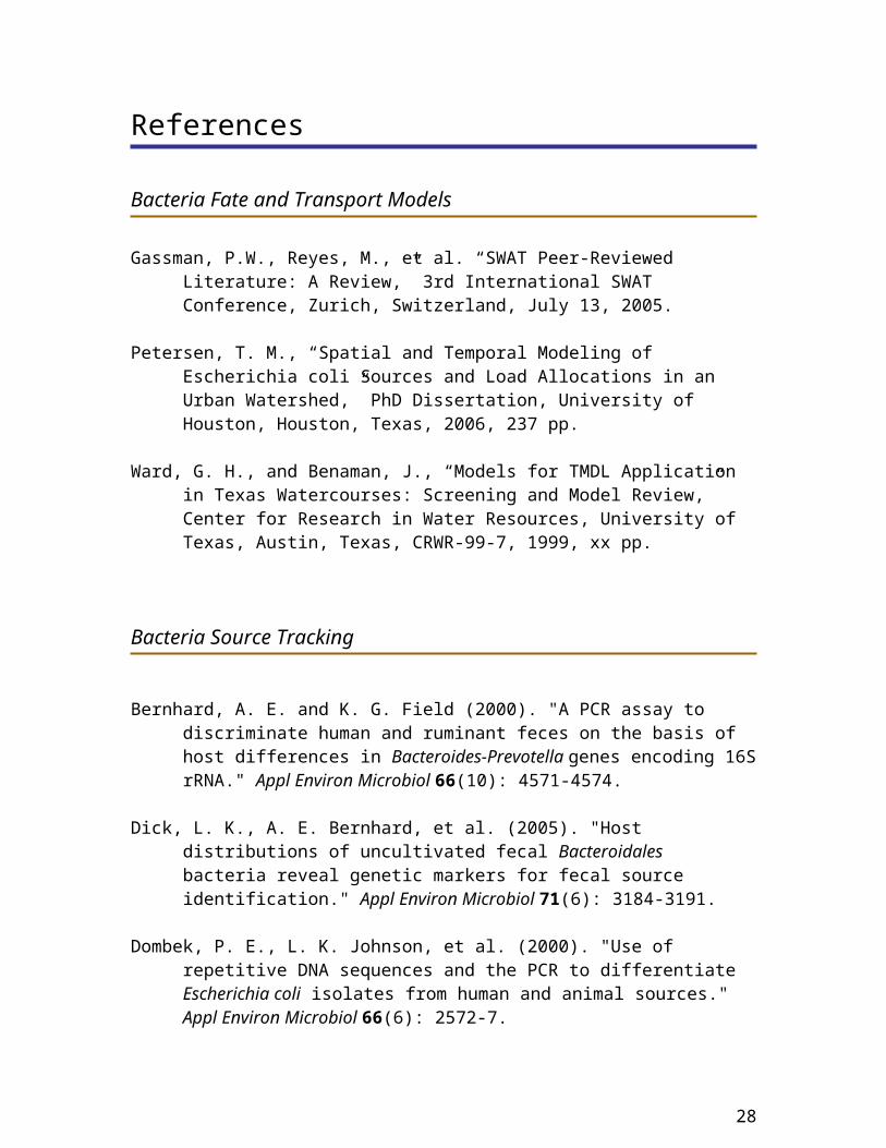
References

Bacteria Fate and Transport Models

Gassman, P.W., Reyes, M., et al. “SWAT Peer-Reviewed Literature: A Review,” 3rd International SWAT Conference, Zurich, Switzerland, July 13, 2005.

Petersen, T. M., “Spatial and Temporal Modeling of Escherichia coli Sources and Load Allocations in an Urban Watershed,” PhD Dissertation, University of Houston, Houston, Texas, 2006, 237 pp.

Ward, G. H., and Benaman, J., “Models for TMDL Application in Texas Watercourses: Screening and Model Review,” Center for Research in Water Resources, University of Texas, Austin, Texas, CRWR-99-7, 1999, xx pp.

Bacteria Source Tracking

Bernhard, A. E. and K. G. Field (2000). "A PCR assay to discriminate human and ruminant feces on the basis of host differences in Bacteroides-Prevotella genes encoding 16S rRNA." Appl Environ Microbiol 66(10): 4571-4574.

Dick, L. K., A. E. Bernhard, et al. (2005). "Host distributions of uncultivated fecal Bacteroidales bacteria reveal genetic markers for fecal source identification." Appl Environ Microbiol 71(6): 3184-3191.

Dombek, P. E., L. K. Johnson, et al. (2000). "Use of repetitive DNA sequences and the PCR to differentiate Escherichia coli isolates from human and animal sources." Appl Environ Microbiol 66(6): 2572-7.

Gordon, D. M., S. Bauer, et al. (2002). "The genetic structure of Escherichia coli populations in primary and secondary habitats." Microbiology 148(5): 1513-1522.

Graves, A. K., C. Hagedorn, et al. (2002). "Antibiotic resistance profiles to determine sources of fecal contamination in a rural Virginia watershed." J Environ Qual 31(4): 1300-1308.

Griffith, J. F., S. B. Weisberg, et al. (2003). "Evaluation of microbial source tracking methods using mixed fecal sources in aqueous test samples." J Water Health 1(4): 141-51.

20

Hamilton, M. J., T. Yan, et al. (2006). "Development of goose- and duck-specific DNA markers to determine sources of Escherichia coli in waterways." Appl Environ Microbiol 72(6): 4012-9.

Hartel, P. G., J. D. Summer, et al. (2003). "Deer diet affects ribotype diversity of Escherichia coli for bacterial source tracking." Water Res 37(13): 3263-8.

Kuntz, R. L., P. G. Hartel, et al. (2003). "Targeted sampling protocol as prelude to bacterial source tracking with Enterococcus faecalis." J Environ Qual 32(6): 2311-2318.

Meays, C. L., K. Broersma, et al. (2004). "Source tracking fecal bacteria in water: a critical review of current methods." J Environ Manage 73(1): 71-79.

Parveen, S., K. M. Portier, et al. (1999). "Discriminant analysis of ribotype profiles of Escherichia coli for differentiating human and nonhuman sources of fecal pollution." Appl. Environ. Microbiol. 65(7): 3142-3147.

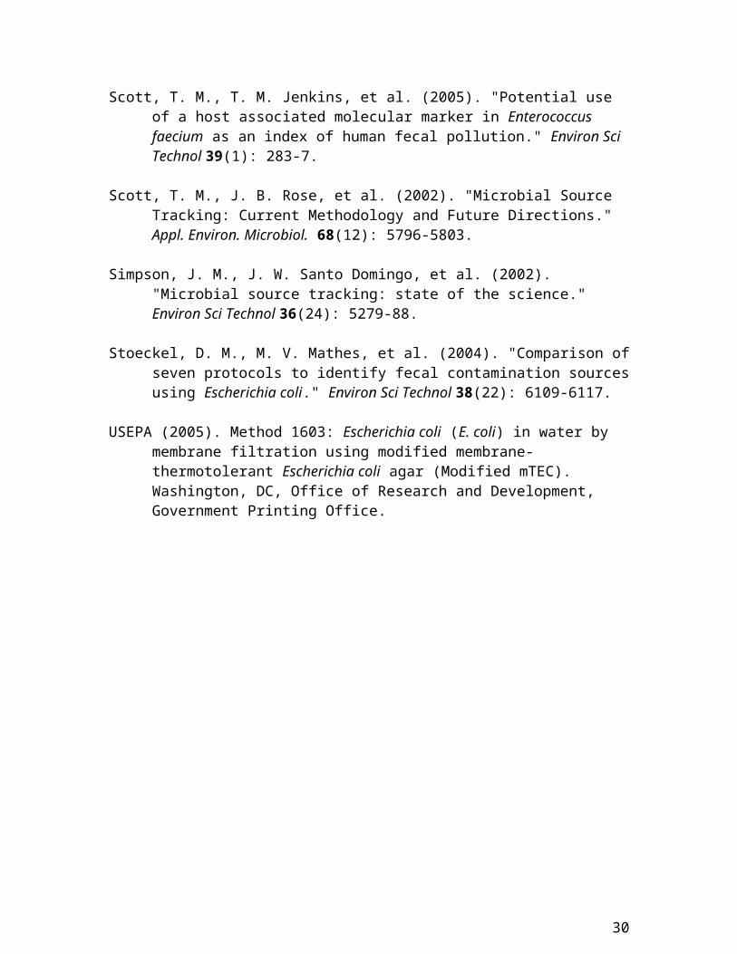
Scott, T. M., T. M. Jenkins, et al. (2005). "Potential use of a host associated molecular marker in Enterococcus faecium as an index of human fecal pollution." Environ Sci Technol 39(1): 283-7.

Scott, T. M., J. B. Rose, et al. (2002). "Microbial Source Tracking: Current Methodology and Future Directions." Appl. Environ. Microbiol. 68(12): 5796-5803.

Simpson, J. M., J. W. Santo Domingo, et al. (2002). "Microbial source tracking: state of the science." Environ Sci Technol 36(24): 5279-88.

Stoeckel, D. M., M. V. Mathes, et al. (2004). "Comparison of seven protocols to identify fecal contamination sources using Escherichia coli." Environ Sci Technol 38(22): 6109-6117.

USEPA (2005). Method 1603: Escherichia coli (E. coli) in water by membrane filtration using modified membrane-thermotolerant Escherichia coli agar (Modified mTEC). Washington, DC, Office of Research and Development, Government Printing Office.

21

Appendix 1: EPA Bacteria TMDL Guidelines

This section provides an overview of several EPA guidance documents related to the use

of models and BST to develop bacteria TMDLs. Components of a TMDL include (1)

Problem Statement, (2) Numeric Targets, (3) Source Assessment, (4) Linkage Analysis,

(5) Allocations, and (6) Monitoring/Evaluation Plan (for phased TMDLs). Because BST

and modeling are primarily used to assist with source assessment, linkage analysis and

allocations, this chapter will focus primarily on these components of the TMDL (EPA

2002a).

Overall, EPA allows a great deal of flexibility in bacteria TMDL development as long as

the method selected adequately identifies the load reductions or other actions needed to

restore the designated uses of the waterbody in question. There are trade-offs associated

with using either simple or detailed approaches. These trade-offs, along with site-specific

factors, should always be taken into account and an appropriate balance struck between

cost and time issues and the benefits of additional analyses (EPA 2002a).

Source Assessment

Source Assessment involves characterizing the type, magnitude and location of sources

of fecal indicator loading. EPA (2002a) encourages starting with the assumption that

models are not required. If it is determined that models are required, then the following

factors should be considered:

Availability of data and/or funds to support data collection

Availability of staff

Familiarity of staff with potential models or other analytical tools

Level of accuracy required

Depending on the complexity of the sources in the watershed, load estimation might be as

simple as conducting a literature search or as complex as using a combination of long-

22

term monitoring and modeling. Analysis of waste loads from point sources are generally

recommended to be based on the effluent monitoring required for the NPDES permit or

on the permit limits (EPA 2002a).

Nonpoint sources loads are typically separated into urban and rural categories since

runoff processes differ between these environments. Pathogen loads in urban storm water

can be estimated using a variety of techniques, ranging in complexity from very simple

loading rate assumptions and constant concentration estimates, to statistical estimates, to

highly complex computer simulation (EPA 2002a). Examples of techniques for

estimating pathogen loads in urban storm water include the FecaLOAD model, constant

concentration estimates, statistical or regression approaches, and storm water models,

such as SWMM and the Hydrological Simulation Program-Fortran (HSPF).

Rural nonpoint source loads may also be estimated using a variety of techniques, ranging

from simple loading function estimates to use of complex simulation models.

Techniques, such as the loading function approach, site-specific analysis, estimates of

time series of loading, and detailed models, such as AGNPS, may be used (EPA 2002a).

Models are discussed in greater depth in the Linkage Analysis section.

DNA fingerprinting may also provide information for Source Assessments (EPA 2002a).

There are many BST methods available and more are under development. Overall,

molecular BST methods may offer the most precise identification of specific types of

sources, but are limited by high costs and detailed, time-consuming procedures (EPA

2002c). Costs vary however, based on:

Analytical method used

Size of the database needed

Number of environmental isolates analyzed

Level of accuracy needed

Comparison studies have shown that no single method is clearly superior to the others.

Thus, the decision on which method to use depends on the unique set of circumstances

23

associated with the area in question, the results of sanitary surveys, and budgetary and

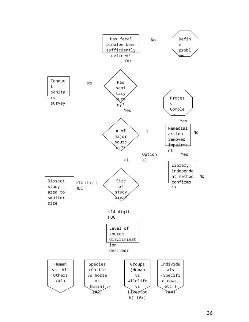
time constraints. A microbial source tracking decision tree was created by EPA to assist

in deciding whether BST methods are necessary to determine the sources of fecal

pollution in a particular watershed and, if so, which group of methods might be most

appropriate (EPA 2005). The decision tree below consists of five steps:

Adequately defining the problem

Conducting a sanitary survey

Determining the potential number of major sources

Ensuring the watershed/study area is of manageable size

Determining the desired level of discrimination

In conclusion, monitoring data should be used to estimate the magnitude of loads from

various sources. In the absence of such data, a combination of literature values, best

professional judgment and empirical techniques/models is necessary. In general, EPA

(2002a) recommends the use of the simplest approach that provides meaningful

predictions.

24

>14 digit HUCNo

Yes>1

No

Yes

1

Has fecal problem been sufficiently

defined?

Define problem

Has sanita

ry surve

y?

No

Yes

Conduct sanitary survey

No

Yes

# of major

sources??

Remedial action removes impairment

Dissect study area to smaller size

Size of study area?

Library independent method confirms 1?

Process Complete

Level of source discrimination desired?

Human vs. All Others

(#1)

Species (Cattle vs horse vs human)

(#2)

Groups (Human vs Wildlife vs Livestock)

(#3)

Individuals (Specific

cows, etc.) (#4)

Optional

<14 digit HUC

25

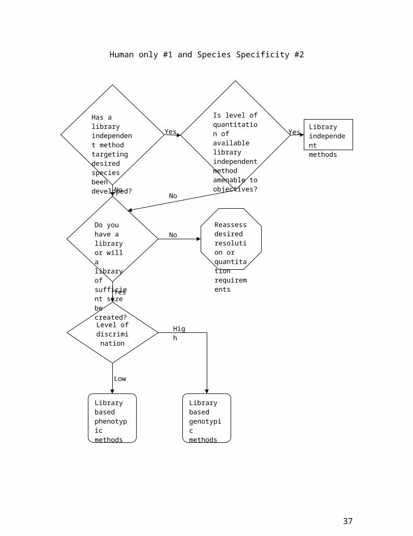
Human only #1 and Species Specificity #2

Yes Yes

NoNo

No

Yes

Low

High

Is level of quantitation of available library independent method amenable to objectives?

Level of discriminatio

n

Reassess desired resolution or quantitation requirements

Library independent methods

Has a library independent method targeting desired species been developed?

Library based phenotypic methods

Do you have a library or will a library of sufficient size be created?

Library based genotypic methods

26

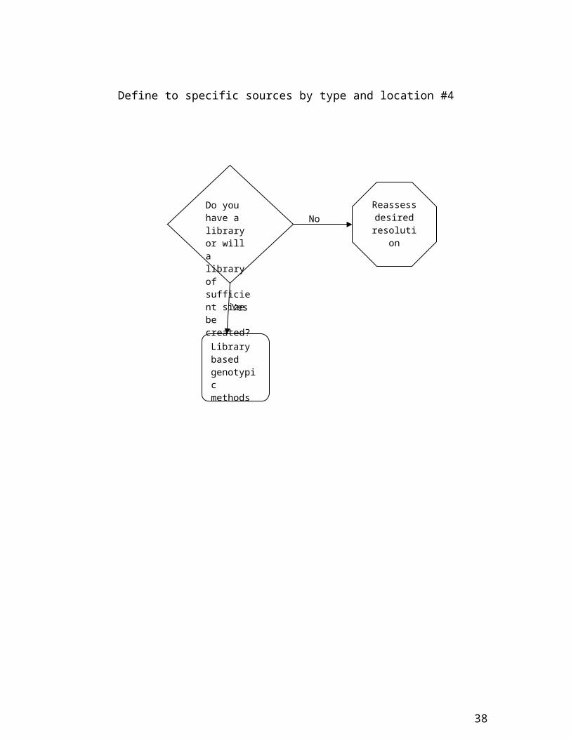
Define to specific sources by type and location #4

Yes

Library based genotypic methods

NoReassess desired

resolution

Do you have a library or will a library of sufficient size be created?

27

Linkage Analysis and Allocations

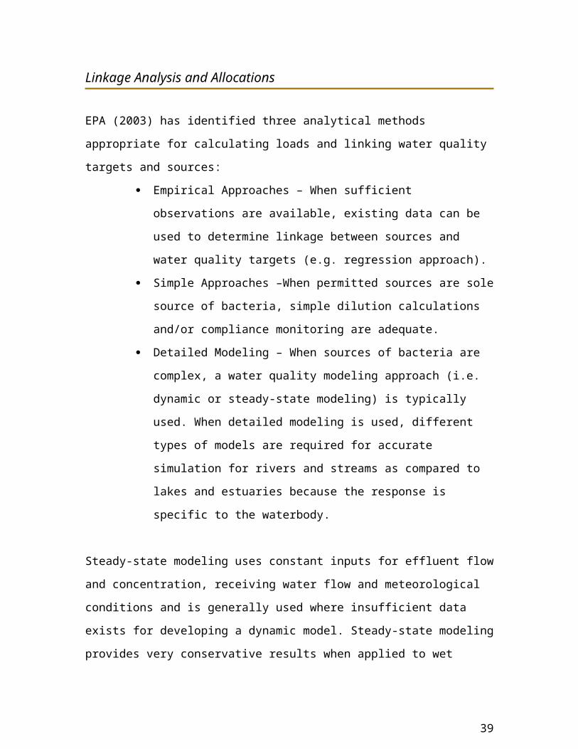
EPA (2003) has identified three analytical methods appropriate for calculating loads and

linking water quality targets and sources:

Empirical Approaches – When sufficient observations are available,

existing data can be used to determine linkage between sources and water

quality targets (e.g. regression approach).

Simple Approaches –When permitted sources are sole source of bacteria,

simple dilution calculations and/or compliance monitoring are adequate.

Detailed Modeling – When sources of bacteria are complex, a water

quality modeling approach (i.e. dynamic or steady-state modeling) is

typically used. When detailed modeling is used, different types of models

are required for accurate simulation for rivers and streams as compared to

lakes and estuaries because the response is specific to the waterbody.

Steady-state modeling uses constant inputs for effluent flow and concentration, receiving

water flow and meteorological conditions and is generally used where insufficient data

exists for developing a dynamic model. Steady-state modeling provides very conservative

results when applied to wet weather sources. If a state elects to use a steady state model,

EPA recommends a dual design approach (i.e. load duration curve) where the loadings

for intermittent or episodic sources are calculated using a flow duration approach and the

loadings for continuous sources are calculated based on a low flow statistic (EPA 2003).

Dynamic modeling considers time-dependent variation of inputs and applies to the entire

record of flows and loadings. EPA (2003) recommends the use of dynamic modeling to

calculate loads. The three dynamic modeling techniques recommended are:

Continuous simulation

Monte Carlo simulation

Log-normal probability modeling

28

Specific models recommended by EPA can be divided into two categories—watershed

loading models and pathogen concentration prediction models. Loading models provide

estimates of either the total pollutant loading or a time series loadings. The key watershed

loading models suited for pathogens include HSPF, SWMM and STORM (EPA 2002b).

These are briefly described in Appendix 3.

Prediction of pathogen concentration in rivers and streams is dominated by advection and

dispersion processes and bacteria die-off. One-, two- and three-dimensional models have

been developed to describe these processes. Waterbody type and data availability are the

two most important factors that determine model applicability. For most small and

shallow rivers, one-dimensional models are sufficient. However, for large and deep rivers

and streams, two- or three-dimensional models that integrate the hydrodynamics of the

system should be used (EPA 2002b). The river and stream models are briefly described in

Appendix 3 and include the following:

HSPF: Hydrological Simulation Program–Fortran

CE-QUAL-RIV1: Hydrodynamic and Water Quality Model for Streams

WASP5: Water Quality Analysis Simulation Program

CE-QUAL-ICM: A Three-Dimensional Time-Variable Integrated-Compartment

Eutrophication Model

EFDC: Environmental Fluid Dynamics Computer Code

CE-QUAL-W2: A Two-Dimensional, Laterally Averaged Hydrodynamic and

Water Quality Model

QUAL2E: The Enhanced Stream Water Quality Model

TPM: Tidal Prism Model

In closing, EPA (2002a) recommends that when developing linkages between water

quality targets and sources, states should:

Use all available and relevant data (specifically monitoring data for associating

waterbody responses with flow and loading conditions).

Perform a scoping analysis using empirical analysis and/or steady-state modeling

to review and analyze existing data prior to any complex modeling. The scoping

29

analysis should include identifying targets, quantifying sources, locating critical

points, identifying critical conditions, and evaluating the need for more complex

analysis.

Use the simplest technique that adequately addresses all relevant factors when

selecting a technique to establish a relationship between sources and water quality

response.

EPA Bacteria TMDL Guidelines References

EPA (Environmental Protection Agency). 2002a. Protocols for Developing Pathogen TMDLs. EPA 841-R-00-002.

EPA (Environmental Protection Agency). 2002b. National Beach Guidance and Required Performance Criteria for Grants. June 2002.

EPA (Environmental Protection Agency). 2002c. Wastewater Technology Fact Sheet – Bacterial Source Tracking. EPA 832-F-02-010.

EPA (Environmental Protection Agency). 2003. Implementation Guidance for Ambient Water Quality Criteria for Bacteria. DRAFT Document.

EPA (Environmental Protection Agency). 2005. Microbial Source Tracking Guide Document. EPA/600-R-05-064.

30

Appendix 2: State Approaches toBacteria TMDL Development

This section provides a brief overview of approaches other states are using to develop

TMDLs for bacteria and related issues. EPA has allowed a great deal of flexibility in

developing pathogen TMDLs, as outlined in the agency’s 2001 publication titled

“Protocols for Developing Pathogen TMDLs” and 2003 DRAFT publication titled

“Implementation Guidance for Ambient Water Quality Criteria for Bacteria.” As a result,

states have taken a variety of approaches to developing bacteria TMDLs. A brief

overview of the processes used by each state in Region 6 and Region 4 along with a few

others is presented here. Much of the information for this summary was acquired from

EPA’s TMDL website found at the following web address:

http://www.epa.gov/owow/tmdl/.

EPA Region 6

In EPA Region 6, 4950 fecal coliform TMDLs are reported to have been approved since

January 1, 1996 as follows:

Arkansas – 2 approved

Louisiana – 27 approved

Oklahoma – 0 approved

New Mexico – 20 approved

Texas – 0 approved

The load duration curve model was the primary model used to develop these TMDLs.

The only exceptions are the two TMDLs developed in Arkansas, which used empirical

methods.

Although no bacteria TMDLs are currently approved in Texas, a number are under way.

The TCEQ TMDL Team has assembled the table below summarizing the modeling and

31

BST methods utilized to develop TMDLs in Texas. Texas has primarily used the HSPF

and load duration curve models for a majority of the TMDLs under development to date.

Project HSPF

Load

Duration Other Models

Bacteria Source Tracking

Method

Upper San Antonio River ERIC-PCR and RiboPrinting

Leon River ERIC-PCR and RiboPrinting

Peach Creek ERIC-PCR and RiboPrinting

Orange CountyAdams and

Cow Bayous

WASP No BST

White Oak and\ Buffalo

Bayous

ARA and CSU

Lower San Antonio River ERIC-PCR and RiboPrinting

Atascosa River No BST

Elm and Sandies Creeks No BST

Upper Trinity River Ribotyping (Washington State

University)

Guadalupe River above

Canyon Lake

Ribotyping (Source Molecular

Corporation, Inc., Miami, FL)

Upper Oyster Creek Ribotyping (Washington State

University)

Copano Bay and Mission

and Aransas Rivers

ArcHydro\Monte

Carlo Simulation

ARP and PFGE

Oso Bay and\ Oso Creek ArcHydro\SWAT No BST

Gilleland Creek No BST

Clear Creek ? ? ? ?

Matagorda Bay (central

Texas Coast oyster waters)

? ? ? ?

Metropolitan Houston

(Brays, Greens, Halls, and

other Bayous)

? ? ? ?

WPP – Plum Creek N Y SELECT,

SPARROW,

SWAT

No BST

WPP – Lake Granbury ? ? ? ?

32

WPP – Buck Creek N TBD TBD E. faecium, ERIC-PCR, RP

WPP – Bastrop Bayou ? ? ? ?

Unlike other states in Region 6, Texas has supplemented the models utilizing Bacteria

Source Tracking. The primary methods that have been used include:

ERIC-PCR conducted at TAES-, El Paso

RiboPrinting conducted at TAES-, El Paso

Antibiotic Resistance Analysis (ARA) conducted at the University of Houston

Carbon Source Utilization (CSU) conducted at the University of Houston

Ribotyping conducted at Washington State University

Ribotyping conducted at Source Molecular Corporation, Inc in Miami, Florida

Antibiotic Resistance Profiling (ARP) conducted at Texas A&M University-,

CCorpus Christi

Pulse Field Gel Electrophoresis (PFGE) conducted at Texas A&M University-,

Corpus Christi

EPA Region 3

In EPA Region 3, 462 fecal coliform, 204 pathogen, and 25 bacteria TMDLs have been

approved as follows:

Delaware – 25 bacteria TMDLs approved

District of Columbia – 22 fecal coliform and 9 pathogen TMDLs approved

Maryland – 57 fecal coliform and 1 pathogen TMDLs approved

Pennsylvania – 100 pathogen and 1 fecal coliform TMDLs approved

Virginia – 186 fecal coliform, 94 pathogen and 1 fecal TMDLs approved.

West Virginia, 196 fecal coliform TMDLs approved.

Information outlining each state’s methodology was not included on EPA’s webpage;

however, a few examples of the methodologies used in specific watersheds in Virginia

and West Virginia were identified and are discussed below.

33

Virginia’s approach is most similar to Texas, in many respects. Virginia develops

bacteria TMDLs primarily using either load duration curves or the HSPF model (or a

modified version – NPSM); however, in a number of TMDLs, BSTbacteria source

tracking has been utilized in conjunction with simplified modeling approaches. A load

duration curve is primarily used to develop both fecal coliform and E. coli TMDLs

addressing the single sample maximum criteria (e.g. Guest River). The HSPF model is

used to develop both fecal coliform and E. coli TMDLs addressing calendar month

geometric mean and single sample maximums (e.g. Linville Creek). In Muddy Creek,

EPA’s BASINS with NPSM, a modified version of HSPF, was used. In Big Otter River,

HSPF was used to estimate current loads. The WLA to point sources allocations were set

at levels equivalent to their permit limits. The NPS allocations were set by source

category for the mainstem and mouths of tributaries and were expressed as fecal coliform

loads per year needed to meet the numeric criteria (ACFW, 2001).

In the Little Wicomico River Watershed TMDL and Coan River Watershed TMDL,

Virginia DEQ utilized its point source inventory, a shoreline survey and antibiotic

resistance analysis to determine the potential sources of bacteria and quantify source

loadings from humans, livestock and wildlife. To develop these TMDLs, a simplified

modeling approach (Tidal Volumetric Model) was used. This simple approach is

applicable to watersheds with small drainage areas, no wastewater treatment plant point

sources, and where land use is not complex. The goal of the procedure is to use BST data

to determine the relative sources of fecal coliform violations and use ambient water

quality data to determine the load reductions needed to attain the applicable criteria. The

most recent 30 months of data coinciding with the end of the TMDL study were reviewed

to determine the loading to the water body. The approach insures compliance with the

90th percentile and geometric mean criteria. The geometric mean loading is based on the

most recent 30-month geometric mean of fecal coliform. The load is also quantified for

the 90th percentile of the 30-month grouping.

The geometric mean load is determined by multiplying the geometric mean concentration

based on the most recent 30-month period of record by the volume of the water. The

34

acceptable load is then determined by multiplying the geometric mean criteria by the

volume of the water. The load reductions needed for the attainment of the geometric

mean are then determined by subtracting the acceptable load from the geometric mean

load.

Example: (Geometric Mean Value MPN/100ml) x (volume) = Existing Load

(Criteria Value 14 MPN/100ml) x (volume) = Allowable Load

Existing Load – Allowable Load = Load Reduction

The 90th percentile load is determined by multiplying the 90th percentile concentration,

based on the most appropriate 30-month period of record, by the volume of the water.

The acceptable load is determined by multiplying the 90th percentile criteria by the

volume of the water. The load reductions needed for the attainment of the 90th percentile

criteria are determined by subtracting the acceptable load from the 90th percentile load.

The more stringent reductions between the two methods (i.e. 90th percentile load or

geometric mean load) are used for the TMDL. The more stringent method is combined

with the results of the BST to allocate source contributions and establish load reduction

targets among the various contributing sources.

The BST data determines the percent loading for each of the major source categories and

is used to determine where load reductions are needed. Since one BST sample per month

is collected for a period of one year for each TMDL, the percent loading per source is

averaged over the 12-month period if there are no seasonal differences between sources.

The percent loading by source is multiplied by the more stringent method (i.e. 90th

percentile load or geometric mean load) to determine the load by source. The percent

reduction needed to attain the water quality standard or criteria are allocated to each

source category.

In West Virginia, BASINS was used by EPA in Alum Run and South Fork of South

Branch of Potomac River. EPA gathered data from local sources to identify, characterize,

and estimate potential fecal coliform loading from various land use categories distributed

35

throughout the Lost River watershed. EPA then used BASINS to develop the TMDL,

using a hydrologically representative time period that captured the varying hydrologic

and climatic conditions in the watershed. Point source loads were estimated using

observed average effluent flow and concentrations where available, or permit limits for

concentration and flow. The watershed was broken down into seven land uses to evaluate

nonpoint sources of bacteria (i.e. barren, cropland, forest, other rural, pasture, residential-

pervious, and residential-impervious).

Failing septic systems were also identified as fecal NPS to the river. BASINS provided

continuous simulation of bacteria buildup and wash off, bacteria loading and delivery,

point source discharge and in stream water quality response and output daily loads from

each land use and point source. Existing loads were established through calibration of the

model to existing water quality data. Loads were reduced until in stream concentrations

met water quality standards.

EPA Region 4

EPA Region 4 is far ahead of EPA Region 6 in developing and approving TMDLs. A

total of 1,146 fecal coliform TMDLs, 175 E. coli TMDLs, 48 fecal TMDLs and 2

pathogen TMDLs are reported to have been approved since January 1, 1996.

Georgia has led the way in TMDL approval with 534 fecal coliform TMDLs approved.

EPA Region 4 completed a number of these (e.g. Chickasawatchee Creek) using the

BASINS model for both source analysis and for linking sources to indicators. No

information was posted on the EPA website regarding Georgia’s methods.

Twenty-one (21) fecal coliform, 45 total coliform, and 48 fecal TMDLs have been

approved in Florida. No information was posted on the EPA website regarding Florida’s

methods.

36

In Kentucky, 23 fecal coliform TMDLs have been approved. At least a third of them

were developed using Mass Balance. The methods used for the other two-thirds were not

reported on the EPA website.

Alabama has had 26 fecal coliform and two pathogen TMDLs approved using a variety

of approaches, including:

Empirical models

Loading Simulation Program in C++ (LSPC), Environmental Fluid Dynamics

Code (EFDC), Water Quality Analysis Simulation Program (WASP)

BASINS Watershed Characterization System (WCS) and Nonpoint Source Model

(a modified version of HSPF)

Mass balance

Load duration curves

Mississippi has completed 172 fecal coliform TMDLs primarily using empirical linear

regression models, BASINS NPSM, and mass balance. The BASINS NPS Model

(NPSM) was used in the Pearl River TMDL, for example, to estimate current conditions.

In this TMDL, point source Waste aLoad Allocations (WLAs) were based on modeled

contributions from municipal WWTPs using monitoring data plus included 50 percent of

estimated septic tank load. NPS Load Aallocations (LAs) were identified on a

subwatershed basis using modeled loads. Gross allotments for each subwatershed

included contributions from direct runoff, septic tanks, cattle grazing, manure application,

urban development and wildlife.

North Carolina has completed 38 fecal coliform TMDLs and 1 fecal TMDL using a

number of models including BASINS HSPF, load duration curves and Watershed

Analysis Risk Framework (WARMF).

Tennessee has completed 62 fecal coliform and 191 E. coli TMDLs utilizing a variety of

models including the BASINS Watershed Characterization System and NPS Model

(NPSM); Loading Simulation Program in C++ (LSPC) / Hydrologic Simulation Program

37

–FORTRAN (HSPF) /Watershed Characterization System (WCS) model combination,

load duration curves and mass balance.

South Carolina has completed 270 fecal coliform TMDLs, primarily using load duration

curves. In limited circumstances, they have also used empirical methods or the

BASINS/HSPF/WSC combo. A “TMDL Talk” on TMDLS.NET titled Watershed

Characterization & Bacteria TMDL’s: South Carolina’s Approach may indicate greater

use of BASINS/HSPF/WSC in coming years. The use of the Watershed Characterization

System (WSC) ensures adequate consideration of the wide array of sources and is a key

component of the technical approach toward building bacteria TMDLs and describing

allocation options. In evaluating pollutant sources, loads are characterized using the best

available information (i.e. monitoring data, GIS data layers, literature values and local

knowledge). Pollutant sources are then linked to water quality targets using analytical

approaches including WCS and the Nonpoint source Model (NPSM), a modified version

of HSPF. Estimates of loading rates are generated by fecal coliform spreadsheet tools

included with WCS. These loading rate estimates are then used by NPSM to simulate the

resulting water quality response. Wasteload Aallocation development for point sources

considers discharge-monitoring information. NPS load allocations for significant

categories are identified at key points in the watershed from the model analyses. This

approach was used for the Rocky Creek TMDL and others.

EPA Region 7

In EPA Region 7, 485 fecal coliform TMDLs, 20 E. coli TMDLs and two pathogen

TMDLs are reported to have been approved since October 1, 1995. Much like EPA

Region 6, load duration curves appear to be the method of choice for developing bacteria

TMDLs. Kansas has lead the way, using load duration curves to develop 471 fecal

coliform TMDLs. In Missouri, three (3) fecal coliform TMDLs, developed using load

duration curves, have been approved by EPA. Similarly, EPA has approved 11 fecal

coliform and 20 E. coli TMDLs in Nebraska, all of which used load duration curves as

38

described in the document entitled “Nebraska’s Approach for Developing TMDLs for

Streams Using the Load Duration Curve Methodology” (NDEQ 2002d).

Only one pathogen TMDL (E. coli) has been approved in Iowa. Iowa used the Soil and

Water Assessment Tool (SWAT) model to estimate daily flow into Beeds Lake. The

SWAT flow estimates were then used to create a load duration curve. Use of EPA’s

bacterial indicator tool was used to identify the significance of bacteria sources in the

watershed.

Other States

Connecticut and Delaware use the Cumulative Frequency Distribution Function Method,

developed by the Connecticut Department of Environmental Protection, to develop

TMDLs. The reduction in bacteria density from current levels needed to achieve

compliance with state water quality standards is quantified by calculating the difference

between the cumulative relative frequency of the sample data set (a minimum of 21

sampling dates during the recreational season) and the criteria adopted to support

recreational use. Adopted water quality criteria for E. coli are represented by a statistical

distribution of the geometric mean 126 and log standard deviation 0.4 for purposes of the

TMDL calculations. TMDLs developed using this approach are expressed as the average

percentage reduction from current conditions required to achieve consistency with

criteria. The procedure partitions the TMDL into wet and dry weather allocations by

quantifying the contribution of ambient monitoring data collected during periods of high

stormwater influence and minimal stormwater influence to the current condition.

Washington primarily uses Load Duration Curves for calculating bacteria TMDLs. To

identify nonpoint sources of bacteria, a yearlong (minimum) water quality study of

possible source areas is conducted. Once the locations of the bacterial sources are

narrowed down, the state works with local interests to identify sources of pollution. Two

methods that can be used to identify bacteria sources: (1) pinpointing the location of the

source and (2) identifying the types of sources contributing to the problem.

39

One of the most economical methods of identifying sources is to conduct intensive

upstream-downstream water quality monitoring, including flow measurements, to

identify specific stream reaches, land uses or tributaries that are a problem. Dye testing

can also be used.

Another method that can be used to determine the types of sources is bacterial source

tracking. Most bacterial source tracking techniques are still in the experimental stage and

are often quite costly; thus, it is important to pick the appropriate time and method to use

BST. It is also important to remember that these techniques do not tell you how much

each source contributes to bacterial contamination, only the different kinds of sources. In

addition, it is possible that not all source types will be identified or, with some

techniques, that sources will be misidentified.

If wildlife is a major source, human related sources must still be reduced. Most bacterial

pollution by wildlife is considered a natural contribution that cannot be controlled.

Rhode Island utilized a simple approach to developing the Hunt River TMDL. The source

assessment was completed by conducting site visits. Wet and dry weather fecal coliform

data were used with frequency distribution of precipitation information to compute a

weighted geometric mean. No point sources were present, thus the load NPS allocations

were expressed as a percent reduction needed to meet the numeric criteria based on a

comparison of current fecal coliform concentrations with the water quality standards

(ACFW, 2001).

40

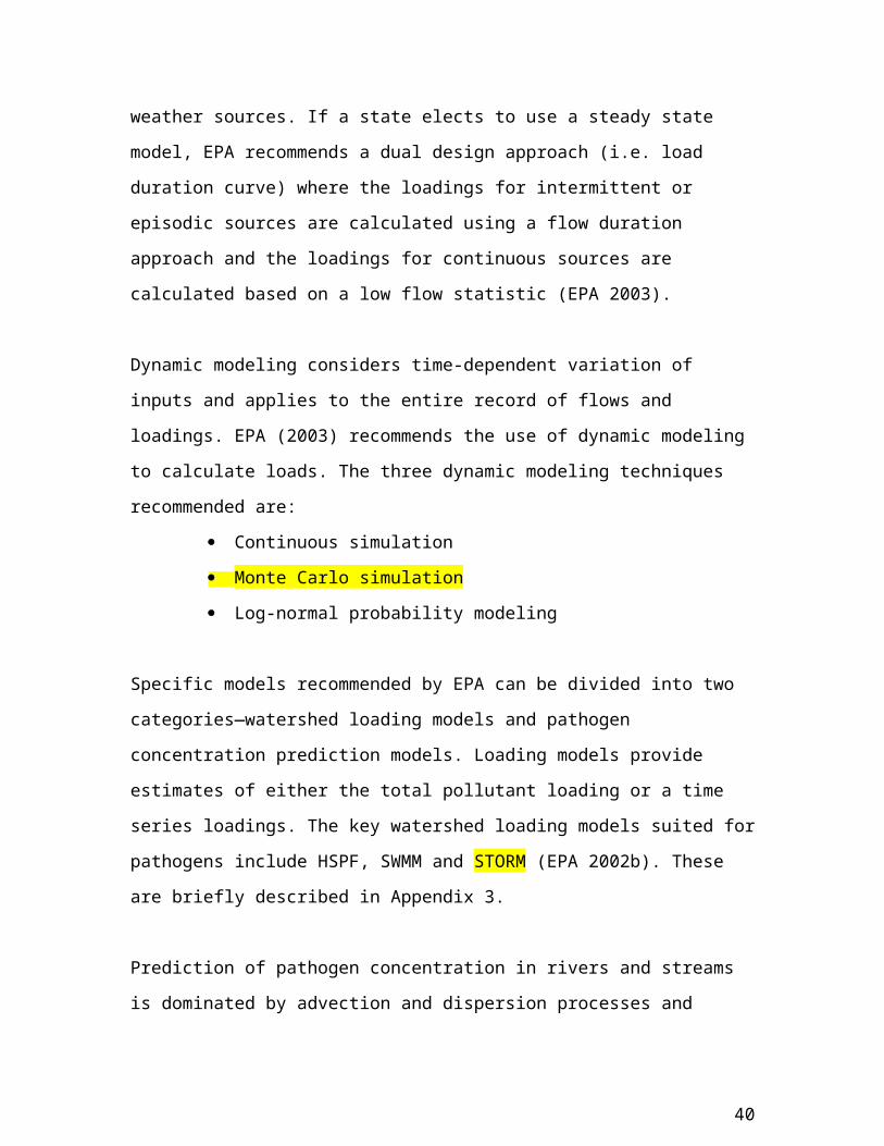
Appendix 3: Models Used in Bacteria Source Tracking as Described in EPA Publications

HSPF: Hydrological Simulation Program—Fortran

HSPF is a comprehensive watershed-scale model developed by EPA. The model uses

continuous simulation of water balance and pollutant buildup and washoff processes to

generate time series of runoff flow rates, as well as pollutant concentration at any given

point in the watershed. Runoff from both urban and rural areas can be simulated using

HSPF; however, simulation of CSOs is not possible. Because of the comprehensive

nature of the model, data requirements for HSPF are extensive and using this model

requires highly trained personnel (EPA 2002b).

SWMM: Storm Water Management Model

SWMM is a comprehensive watershed-scale model developed by EPA. It can be used to

model several types of pollutants on either a continuous or storm event basis. Simulation

of mixed land uses is possible using SWMM, but the model’s capabilities are limited for

rural areas. SWMM can simulate loadings from CSOs. The model requires both intensive

data input and a special effort for validation and calibration. The output of the model is

time series of flow, storage and contaminant concentrations at any point in the watershed

(EPA 2002b).

STORM: Storage, Treatment, Overflow, Runoff Model

STORM is a watershed-loading model developed by the U.S. Army Corps of Engineers

for continuous simulation of runoff quantity and quality. The model was primarily

designed for modeling storm water runoff from urban areas, but it also can simulate

combined sewer systems. It requires relatively moderate to high calibration and input

data. The simulation output is hourly hydrographs and pollutographs (EPA 2002b).

41

CE-QUAL-RIV1: Hydrodynamic and Water Quality Model for Streams

CE-QUAL-RIV1 is a dynamic, one-dimensional model for rivers and estuaries consisting

of two codes—one for hydraulic routing and another for dynamic water quality

simulation. CE-QUAL-RIV1 allows simulation of unsteady flow of branched river

systems. The input data requirements include the river geometry, boundary conditions,

initial in-stream and inflow boundary water quality concentrations and meteorological

data. The model predicts time-varying concentrations of water quality constituents (EPA

2002b).

Predicting the response of lakes and estuaries to pathogen loading requires an

understanding of the hydrodynamic processes. Shallow lakes can be simulated as a

simplified, completely mixed system with an inflow stream and an outflow stream.

However, simulating deep lakes or estuaries with multiple inflows and outflows that are

affected by tidal cycles is not a simple task. Pathogen concentration prediction is

dominated by the processes of advection and dispersion, and these processes are affected

by the tidal flow. The size of the lake or the estuary, the net freshwater flow, and wind

conditions are some of the factors that determine the applicability of the models. The lake

and estuary models are briefly described below (EPA 2002b).

WASP5: Water Quality Analysis Simulation Program

WASP5 is a general-purpose modeling system for assessing the fate and transport of

pollutants in surface water. The model can be applied in one, two or three dimensions and

can be linked to other hydrodynamic models. WASP5 simulates the time-varying

processes of advection and dispersion while considering point and nonpoint source

loadings and boundary exchange. The waterbody to be simulated is divided into a series

of completely mixed segments, and the loads, boundary concentrations, and initial

concentrations must be specified for each state variable (EPA 2002b).

42

CE-QUAL-ICM: A Three-Dimensional Time-Variable Integrated-Compartment Eutrophication Model

CE-QUAL-ICM is a dynamic water quality model that can be applied to most

waterbodies in one, two or three dimensions. The model can be coupled with three-

dimensional hydrodynamic and benthic-sediment model components.

CE-QUAL-ICM predicts time-varying concentrations of water quality constituents. The

input requirements for the model include 140 parameters to specify the kinetic

interactions, initial and boundary conditions, and geometric data to define the waterbody

to be simulated. Model use might require significant expertise in aquatic biology and

chemistry (EPA 2002b).

EFDC: Environmental Fluid Dynamics Computer Code

EFDC is a general three-dimensional hydrodynamic model developed by Hamrick

(1992). EFDC is applicable to rivers, lakes, reservoirs, estuaries, wetlands and coastal

regions where complex water circulation, mixing and transport conditions are present.

EFDC must be linked to a water quality model to predict the receiving water quality

conditions. HEM-3D is a three-dimensional hydrodynamic eutrophication model that was

developed by integrating EFDC with a water quality model. Considerable technical

expertise in hydrodynamics and eutrophication processes is required to use the EFDC

model (EPA 2002b).

CE-QUAL-W2: A Two-Dimensional, Laterally Averaged Hydrodynamic and Water Quality Model

CE-QUAL-W2 is a hydrodynamic water quality model that can be applied to most

waterbodies in one dimension or laterally averaged in two dimensions. The model is

suited for simulating long, narrow waterbodies like reservoirs and long estuaries, where

43

stratification might occur. The model application is flexible because the constituents are

arranged in four levels of complexity. Also, the water quality and hydrodynamic routines

are directly coupled, allowing for more frequent updating of the water quality routines.

This feature can reduce the computational burden for complex systems. The input

requirements for CE-QUAL-W2 include geometric data to define the waterbody, specific

initial boundary conditions and specification of approximately 60 coefficients for the

simulation of water quality (EPA 2002b).

QUAL2E: The Enhanced Stream Water Quality Model

QUAL2E is a steady-state receiving water model. The basic equation used in QUAL2E is

the one-dimensional advective-dispersive mass transport equation. Although the model

assumes a steady-state flow, it allows simulation of diurnal variations in meteorological

inputs. The input requirements of QUAL2E include the stream reach physical

representation and the chemical and biological properties for each reach (EPA 2002b).

TPM: Tidal Prism Model

TPM is a steady-state receiving water quality model applicable only to small coastal

basins. In such locations, the tidal cycles dominate the mixing and transport of pollutants.

The model assumes that the tide rises and falls simultaneously throughout the waterbody

and that the system is in hydrodynamic equilibrium. Two types of input data are required

to run TPM. The geometric data that define the system being simulated are the returning

ratio, initial concentration and boundary conditions. The physical data required are the

water temperature, reaction rate, point and nonpoint sources, and initial boundary

conditions for water quality parameters modeled (EPA 2002b).

BASINS: Better Assessment Science Integrating Point and Nonpoint Sources

44

BASINS system Version 2.0, with the Nonpoint Source Model (NPSM), can be used to

predict the significance of fecal coliform sources and fecal coliform levels watersheds.

BASINS is a multipurpose environmental analysis system for use in performing

watershed and water quality-based studies. A geographic information system (GIS)

provides the integrating framework for BASINS and allows for the display and analysis

of a wide variety of landscape information (e.g., land uses, monitoring stations, point

source discharges). The NPSM model within BASINS simulates nonpoint source runoff

from selected watersheds, as well as the transport and flow of the pollutants through

stream reaches. Through calibration of model parameters and representation of watershed

sources, the transport and delivery of bacteria to watershed streams and the resulting in-

stream response and concentrations were simulated (EPA 2002a).

Models Used in Bacteria Source Tracking asDescribed in EPA Publications References

EPA (Environmental Protection Agency). 2002a. Protocols for Developing Pathogen TMDLs. EPA 841-R-00-002.

EPA (Environmental Protection Agency). 2002b. National Beach Guidance and Required Performance Criteria for Grants. June 2002.

45

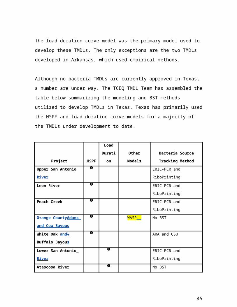
Appendix 4: Bacterial TMDL Task Force Personnel

Members

Allan Jones (Chair) Texas Water Resources InstituteGeorge Di Giovanni Texas Agricultural Experiment Station - El PasoLarry Hauck Tarleton State University/Texas Institute for Applied Environmental ResearchJoanna Mott Texas A&M University-Corpus ChristiHanadi Rifai University of HoustonRaghavan Srinivasan Texas A&M University- Spatial Sciences LaboratoryGeorge Ward University of Texas at Austin

Expert Advisors

Faith Hambleton TCEQJim Davenport TCEQPatrick Roques TCEQAndrew Sullivan TCEQJohn Foster TSSWCBAaron Wendt TSSWCBDuane Schlitter TPWDMonica Kingsley DSHSKirk Wiles DSHSRichard Eyster TDADavid Villarreal TDANed Meister Texas Farm BureauJohn Barrett Agriculture Producer / LandownerJohn Blount City of HoustonGreg Rothe San Antonio River AuthorityWiley Stem City of WacoFred Cox Hamilton CountyRandy Rush USEPA – Region 6 – NPS GrantsShawneille Campbell USEPA – Region 6 – TMDLMike Schaub USEPA – Region 6 – Ecosystems Branch?Bob Joseph USGSMyron Hess Environmental Groups (National Wildlife Federation)Mel Vargas Consulting Firms (Parsons)David Harkins Consulting Firms (Espey?)James Miertschin Consulting Firms (JMA)Terry Gentry TAMU-Soil & Crop Sciences?

46

Tom Edrington USDA-Agricultural Research Service?David Maidment UT CRWRRichard Hay TAMU-CC CWSSDave Bass LCRAs

Agency Staff

Ashley Wadick TCEQBetsy Chapman TCEQElaine Lucas TCEQJohn Foster TSSWCBJason Skaggs TCEQKevin Wagner TWRIRosemary Payton TWRI

47

Appendix 5: Comments from Expert Advisory Group

Texas Parks and Wildlife Department's Role in the Bacterial TMDL Process

Texas Parks and Wildlife Department ("the Department") is the state agency with

primary responsibility for protecting the state's fish and wildlife resources (Parks and

Wildlife Code §12.0011(a)). Further, the Department is tasked with providing

information on fish and wildlife resources to entities that make decisions affecting those

resources (Parks and Wildlife Code §12.0011(b)(3)).

Texas Parks and Wildlife Department has purview over the wild animals, wild birds, and

aquatic animal life of the state (Parks and Wildlife Code §61.005). The Department's

authority extends, through the definition of "wildlife," to any wild mammal, animal, wild

bird, or any part, product, egg, or offspring, of any of these, dead or alive (Parks and

Wildlife Code §68.001).

The Department's authority is limited to indigenous species through the definition of

"wild.” Exotic livestock is specifically excluded. "Wild," when used in reference to an

animal, means a species, including each individual of a species that normally lives in a

state of nature and is not ordinarily domesticated. This definition does not include exotic

livestock defined by Section 161.001(a)(4), Agriculture Code (Parks and Wildlife Code

§1.101). The Agriculture Code defines "exotic livestock" as grass-eating or plant-eating,

single-hooved or cloven-hooved mammals that are not indigenous to this state and are

known as ungulates, including animals from the swine, horse, tapir, rhinoceros, elephant,

deer, and antelope families (Agriculture Code §161.001(a)(4)). Thus, certain species,

such as feral swine, axis deer, and sika deer, do not fall within the scope of the

Department's authority to protect or manage.

48

The Department recognizes that water is the basis for a significant recreational resource

in Texas that includes boating, fishing, swimming, sailing, diving, bird watching and

paddle sports (Texas Parks and Wildlife Department, Land and Water Conservation and

Recreation Plan, Recreation Priorities on Texas Waters, pg. 64). As such, the Department

has established as one of its major goals to maintain or improve water quality and

quantity to support the needs of fish, wildlife and recreation (Texas Parks and Wildlife

Department, Land and Water Conservation and Recreation Plan, Goal 7, pg. 75). The

Department recognizes that the Texas Commission on Environmental Quality ("the

Commission") is the state agency with primary responsibility for protecting water quality

(Water Code §26.011). The Department supports the Commission's efforts to improve

and restore water quality through the Total Maximum Daily Load (TMDL) process.

Within the scope of its authority, as outlined above, the Department is committed to

assisting the Commission and the Texas State Soil and Water Conservation Board ("the

Board") in their efforts to restore full use of waterbodies for which the contact recreation

use is impaired.

Specific Comments

1. "Begin with the end in mind.” In order to assist in restoring impaired waterbodies, it is

important to develop data that are useful to the stakeholders who will ultimately

implement the recommended best management practices. This may mean different things

to different stakeholders.

2. One of the tools available to the Department is to assist private landowners in

developing habitat management plans. These plans contain a comprehensive treatment of

past and existing management and habitat conditions, existing wildlife species to be

managed, list of landowner goals, and management recommendations that detail how to

achieve those goals on a specific parcel. In order to develop such plans, there is a need to

have species-specific information about contributions to bacterial loads. At present, the

TMDL process does not provide the information the Department would need.

49

3. The approach currently taken in bacterial source tracking (BST) studies needs

refinement. Overall, the point source library needs to be extended to include more taxa

with rigorously collected samples with adequate replication for each species.

a) Field sampling methods need to be improved. We understand that at least

some samples have been collected from deposited fecal matter. This provides

opportunity for contamination. The Department would recommend killing and

gutting specimens to avoid the potential for contamination.

b) It is not clear that the BST library sampling is adequate from a statistical

design perspective. We believe that the library lacks adequate replication. With

the information available to us now about bacterial strains and promiscuity, we

would recommend that ten or more samples be collected for each species, e.g. ten

samples of great blue herons, ten samples of American egrets, etc.

c) In developing the library, it is important to have a sense of the species in

each watershed that may be contributing the largest bacterial load to the

waterbody. In general, one would expect these to be the species that spend time

on or near the water. These are not necessarily the largest species in the

watershed, nor would they necessarily be the species with the greatest biomass in

the watershed.

50