Back to BaySICS: A User-Friendly Program for Bayesian Statistical Inference from Coalescent Simulations

Back to BaySICS: A User-Friendly Program for BayesianStatistical Inference from Coalescent SimulationsEdson Sandoval-Castellanos1,2*, Eleftheria Palkopoulou1,2, Love Dalen1

1 Department of Bioinformatics and Genetics, Swedish Museum of Natural History, Stockholm, Sweden, 2 Department of Zoology, Stockholm University, Stockholm,

Sweden

Abstract

Inference of population demographic history has vastly improved in recent years due to a number of technological andtheoretical advances including the use of ancient DNA. Approximate Bayesian computation (ABC) stands among the mostpromising methods due to its simple theoretical fundament and exceptional flexibility. However, limited availability of user-friendly programs that perform ABC analysis renders it difficult to implement, and hence programming skills are frequentlyrequired. In addition, there is limited availability of programs able to deal with heterochronous data. Here we present thesoftware BaySICS: Bayesian Statistical Inference of Coalescent Simulations. BaySICS provides an integrated and user-friendlyplatform that performs ABC analyses by means of coalescent simulations from DNA sequence data. It estimates historicaldemographic population parameters and performs hypothesis testing by means of Bayes factors obtained from modelcomparisons. Although providing specific features that improve inference from datasets with heterochronous data, BaySICSalso has several capabilities making it a suitable tool for analysing contemporary genetic datasets. Those capabilities includejoint analysis of independent tables, a graphical interface and the implementation of Markov-chain Monte Carlo withoutlikelihoods.

Citation: Sandoval-Castellanos E, Palkopoulou E, Dalen L (2014) Back to BaySICS: A User-Friendly Program for Bayesian Statistical Inference from CoalescentSimulations. PLoS ONE 9(5): e98011. doi:10.1371/journal.pone.0098011

Editor: David Caramelli, University of Florence, Italy

Received November 12, 2013; Accepted April 28, 2014; Published May 27, 2014

Copyright: � 2014 Sandoval-Castellanos et al. This is an open-access article distributed under the terms of the Creative Commons Attribution License, whichpermits unrestricted use, distribution, and reproduction in any medium, provided the original author and source are credited.

Funding: This work was supported by Formas via the ERA-NET Biodiversa project Climigrate and the Strategic Research Programme Ekoklim at StockholmUniversity. It received also funding from the Swedish Research Council and EP acknowledges funding from Stiftelsen Lars Hiertas Minne, as well as the project ‘‘IKYscholarships’’ financed by the operational program ‘‘Education and Lifelong Learning’’ of the European Social Fund (ESF) and the NSRF 2007-2013. The fundershad NO role in study design, data collection and analysis, decision to publish, or preparation of the manuscript.

Competing Interests: The authors have declared that no competing interests exist.

* E-mail: [email protected]

Introduction

The power of population genetics and genomics to infer past

evolutionary processes has vastly increased in the last 30 years due

to the synergy created by highly influential advances, both

theoretical (coalescent theory, Bayesian statistics) and technolog-

ical (high throughput sequencing, high performance computers,

ancient DNA analysis) [1], [2], [3].

While coalescent theory has created a simple, powerful, and

elegant way to model evolutionary processes [1], [4], Bayesian

statistics have provided a solid theoretical framework for the

treatment of complex systems as well as for inference based on

computer simulations [5], [6], [7]. Furthermore, sequencing of

large genomic regions has significantly enhanced statistical power

due to larger nucleotide sampling [3], [8], [9]. In addition, the

recent progress made in the field of ancient DNA has provided the

opportunity to directly trace microevolutionary changes in

macrobiotic systems [10], [11].

The most relevant advances in statistical inference have been

brought about by the diversification and refinement of Monte

Carlo methods, usually exploited by Bayesian methodologies. The

most successful technique used for Bayesian inference is the

Markov chain Monte Carlo (MCMC) [6]. Despite their success,

MCMC methods suffer from known limitations when systems

become highly complex, since the calculation of likelihoods, which

is indispensable for its implementation, becomes difficult or

impossible [12], [13], (but see [14]).

Approximate Bayesian computation (ABC) stands among the

most promising Monte Carlo techniques [2], [6], [12], and is

increasing in popularity due to its simple fundament and

exceptional flexibility, enabled by its likelihood-free implementa-

tion [13]. Applications of ABC range from assessing models in

human evolution [15], [16], estimating the rate of spread in

pathogens [17], [18], to estimation of mutation rates [19],

migration rates [20], selection rates [21], and population

admixture [22]. In the case of studies that include ancient DNA

data, ABC has been successfully used to link environmental events

with population structuring [23], [24], past migration events [25],

and extinction [26]. Moreover, ABC has been suggested for

applications beyond the field of population genetics [12], [13].

Despite its recognized potential, ABC also accounts for well

identified challenges, including the necessity for validation and

adjustment [2], [12], [13], [27], the choice of summary statistics

that are Bayes sufficient (i.e. that fully capture the information

contained in the data) [12], [28], and the unreliability in model

choice [28], [29]. However, perhaps the most important downside

of the ABC method is its low computational efficiency [30].

Many efforts have been made to provide tools that improve the

computational efficiency of the analysis [2], [14], [30], [31], [32],

[33], as well as to establish a user-friendly interface for wider use

[27], [34], [35], [36], [37]. However, the number of options is still

PLOS ONE | www.plosone.org 1 May 2014 | Volume 9 | Issue 5 | e98011

limited for evolutionary studies employing heterochronous data.

For instance, at present, there is only one program available that

provides a single platform for performing simulations, rejection

procedures and posterior probabilities estimations for heterochro-

nous data (DIYABC; [38]).

Here we present the software BaySICS: Bayesian Statistical

Inference of Coalescent Simulations. A Windows program that

provides an integrated and user-friendly platform to perform

coalescent simulations for DNA sequence data and ABC analysis

including estimation of posterior densities for population param-

eters and Bayes factors for model comparisons. BaySICS

implements a number of tools for improving the simulations and

interpretation of results, including novel summary statistics specific

for ancient DNA data, 2-D and 3-D graphics, as well as an

MCMC-without-likelihoods algorithm.

Materials and Methods

The softwareBaySICS comprises a set of three independent programs that

are managed by a common graphical interface. The first program

executes coalescent simulations, the second program performs the

post-simulation analysis, and the third program performs valida-

tion procedures based on pseudo-observed data sets (PODs).

The first program generates simulated samples corresponding in

number, ages and population assignment (if applicable) to the

observed ones, under a population history that is fully specified in

an input file. It can simulate non-recombining DNA from a locus

that is autosomal haploid, diploid or haplo-diploid (X-linked), as

well as an Y-linked or mitochondrial. The simulation design

consists of an assembly of coalescing blocks, rather than events,

delimited by specific time bounds. Each block coalesces lineages

from one or two sources (populations or blocks), which permits the

simulation of any historical population structure, including

populations that merge and split in time. Each block contains its

own effective population size (Ne) and growth rate. Ages of the

samples, Ne, growth rate, age of a block (equivalent to the age of an

event), migration rates, proportion of lineages sourced to a block,

generation time, mutation rates, gamma parameter (shape), and

transition/transversion bias, are parameters that can be drawn

from prior densities. The summary statistics estimated for each

simulated data set include the number of total and private

haplotypes, gene and nucleotide diversities, FST, average number

of pairwise differences (within and between populations) and

Tajima’s D. Moreover, multi-dimensional summary statistics can

be calculated and employed, such as mismatch distributions,

Neighbour-Joining trees and the matrix of pairwise differences

among sequences. For heterochronous genetic data, we have

further included a novel temporally weighted matrix of pairwise

differences. In this matrix, the temporal distances among

individuals determine the weight of their pairwise differences,

with large temporal distances contributing less to the inference.

This summary statistic is useful for tracking demographic changes

through time when heterochronous samples with a large temporal

coverage are included. The rationale behind this approach is that

in studies with wide temporal coverage, the tracking of

demographic change through time is improved by discarding

information that becomes meaningless due to an excessive

temporal separation among samples.

The post-simulation analysis program performs two types of

analyses: parameter estimation and model comparison. Both can

be performed employing different tables obtained independently

and integrated into a single analysis, which provides flexibility for

parallelizing the simulations.

The parameter estimation algorithm follows the one proposed

by Beaumont et al. [2]. In BaySICS it consists of: i) reading the

summary statistics and parameters from one or more reference

tables; ii) applying the rejection procedure (see next paragraph); iii)

adjusting and estimating the posterior densities of the parameters

with optional regression and kernel procedures as described in [2];

iv) displaying and saving the posteriors of the parameters of interest

(including joint posteriors if required); and v) displaying optional

charts of the predictive distributions of the summary statistics.

Most of the available software for ABC analyses performs model

comparisons by choosing a target number of simulations that have

the shortest Euclidean distances to the observed summary

statistics. This method, from here on called the proportion

method, bypasses the problematic necessity to define an appro-

priate threshold for rejection. However, when too many summary

statistics are employed, a high dimensionality phenomenon can

occur, in which a small Euclidean distance (calculated over all the

summary statistics) could be accompanied by not-so-small

individual distances in some of the summary statistics. In other

words, if many summary statistics are employed it is possible that

the accepted simulations give values that could be considered

unacceptable for some summary statistics although their overall

Euclidean distance is still among the shortest ones. If some

summary statistics should be kept under an acceptable range, a

definition of acceptance thresholds for all the summary statistics

could be preferable over the proportion method. BaySICS can

perform both methods and, for model choice analysis, repeats the

analysis 50 times for different proportions or thresholds in order to

assess the consistency of the acceptance ratios at different tolerance

levels. The ratios of the different models in the accepted sample is

then interpreted as an estimation of the models likelihoods from

which it is straightforward to estimate Bayes factors. The

procedure can also be improved by applying a logistic regression,

also implemented in BaySICS, where the summary statistics are

seen as explanatory variables of the model likelihoods in a

neighbourhood of the observed values [15].

The calculation of distances between the summary statistics of

observed and simulated data is an essential step in the post-

simulation analysis. The standard distance is the Euclidean

distance:

L(s0,ss)~P

(xi{yi)2

� �1=2, s0~(x1,x2,:::); ss~(y1,y2,:::),

where so and ss are the vectors of summary statistics in the

observed and simulated alignments respectively. This distance is

usually normalized by the standard deviation of the simulated

values [2], [38], in order to counteract the effect of the very

different scales that summary statistics can have; for instance the

number of segregating sites could be seven orders of magnitude

larger than nucleotide diversity. BaySICS employs the difference

between the median of the simulated data and the observed value

as the normalizing factor, instead of the standard deviation,

because this promotes a balanced contribution of every summary

statistic in circumstances where other normalizing factors fail to do

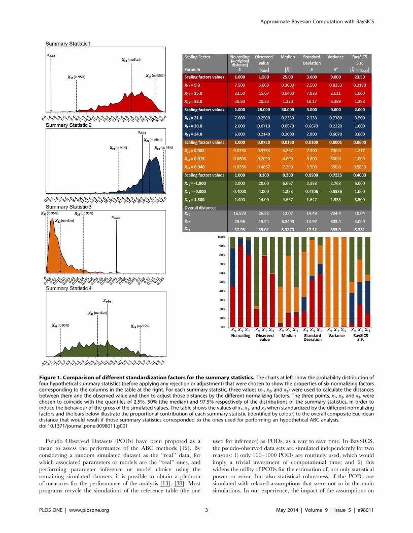
so. For instance, the examples used in figure 1, show that using the

observed value as a standardizing factor produces an overrepre-

sentation of summary statistics 1 and 4 (red and green) in the

Euclidean distance because the observed value was small

compared to most of the simulated values. Standard deviation

also has the disadvantage of neglecting the observed value, such

that a large difference between the observed value and the

simulated ones (in comparison to the standard deviation) will make

the distances large (see summary statistic 1 in red; figure 1). The

standardizing factor implemented in BaySICS has the advantage

of normalizing to equal values the distances of the most frequent

simulated values: the ones around the median.

Approximate Bayesian Computation with BaySICS

PLOS ONE | www.plosone.org 2 May 2014 | Volume 9 | Issue 5 | e98011

Pseudo Observed Datasets (PODs) have been proposed as a

mean to assess the performance of the ABC methods [12]. By

considering a random simulated dataset as the ‘‘real’’ data, for

which associated parameters or models are the ‘‘real’’ ones, and

performing parameter inference or model choice using the

remaining simulated datasets, it is possible to obtain a plethora

of measures for the performance of the analysis [13], [38]. Most

programs recycle the simulations of the reference table (the one

used for inference) as PODs, as a way to save time. In BaySICS,

the pseudo-observed data sets are simulated independently for two

reasons: 1) only 100–1000 PODs are routinely used, which would

imply a trivial investment of computational time; and 2) this

widens the utility of PODs for the estimation of, not only statistical

power or error, but also statistical robustness, if the PODs are

simulated with relaxed assumptions that were not so in the main

simulations. In our experience, the impact of the assumptions on

Figure 1. Comparison of different standardization factors for the summary statistics. The charts at left show the probability distribution offour hypothetical summary statistics (before applying any rejection or adjustment) that were chosen to show the properties of six normalizing factorscorresponding to the columns in the table at the right. For each summary statistic, three values (x1, x2, and x3) were used to calculate the distancesbetween them and the observed value and then to adjust those distances by the different normalizing factors. The three points, x1, x2, and x3, werechosen to coincide with the quantiles of 2.5%, 50% (the median) and 97.5% respectively of the distributions of the summary statistics, in order toinduce the behaviour of the gross of the simulated values. The table shows the values of x1, x2, and x3 when standardized by the different normalizingfactors and the bars below illustrate the proportional contribution of each summary statistic (identified by colour) to the overall composite Euclideandistance that would result if those summary statistics corresponded to the ones used for performing an hypothetical ABC analysis.doi:10.1371/journal.pone.0098011.g001

Approximate Bayesian Computation with BaySICS

PLOS ONE | www.plosone.org 3 May 2014 | Volume 9 | Issue 5 | e98011

the results is a primary source of concern in the application of

statistical inference to evolutionary studies. A PODs analysis can

be employed in BaySICS for estimating the rate of false positives

or false negatives in a model choice analysis, which could be

interpreted as statistical power or error type I-II, as well as to

obtain measures of the performance in a parameter estimation

analysis. Performance measures include the mean relative bias, the

square root of the relative mean square error (RRMSE), the 50%

and 95% coverage, and the factor 2 [38].

BaySICS also implements an MCMC-without-likelihoods pro-

cedure (MCMCwL). This procedure follows Marjoram et. al [14]

and performs a pre-run of 10,000 simulations to estimate a

threshold that accepts 1% of the simulations and then use that

threshold to reject on-the-go the simulations with probability

equivalent to the ratio of the transition kernel evaluated in the

current state and the newly proposed one [14]. The transition

kernel is settled to a normal density with a S.D. being one tenth of

the range of the parameter in the prior. The reference table that is

obtained by this type of analysis lists the chosen summary statistics

and the simulations that were accepted on-the-go with an

acceptance threshold that would retain approximately 1% of the

most similar simulations (to the observed data) in a normal run.

Validation and TestsTo assess the features and performance of BaySICS, we carried

out an evaluation at three levels: 1) a qualitative assessment; 2) a

comparison with theoretical predictions; and 3) an estimation of

measures of performance by means of PODs.

The qualitative assessment consisted of a subjective comparison

of the features of the software after performing complete analyses

on simulated data that were inspired by real case studies. The

complete analyses included setting up and running the coalescent

simulations to performing parameter estimation and model

comparisons. For parameters estimation a relatively complex

model was employed including a population structure of three

populations, two splits events and nine unknown parameters while

the model comparison assessed four hypotheses of demographic

history in four time periods (see figure S1).

Theoretical predictions were assessed by using a group of test

examples for which the expectations of the times to the first,

second, etc. coalescences; the expectation of the time to the most

recent common ancestor (TMRCA), and the expectation of the tree

length were calculated according to the formulas in [39]. The

theoretical expectations were compared with the average values

obtained from 10 000 simulations ran under the same scenario

and parameter values with two software options: BaySICS and

Bayesian Serial Simcoal (BSSC) [40]. In the case of BSSC only

TMRCA was obtained. The employed test examples included simple

scenarios where formulas could be applied in a more or less

straightforward way (see table S1). In addition, the estimated

summary statistics were compared to the ones obtained from other

software (Arlequin [41]). Posterior and predictive distributions

obtained by MCMCwL were also compared with the ones

obtained by an ordinary analysis without MCMCwL.

The performance measurements were obtained by running sets

of 10 000 PODs. PODs were obtained by simulating datasets with

different combinations of parameter values to assess at once the

expected performance of the estimations for a range of parameter

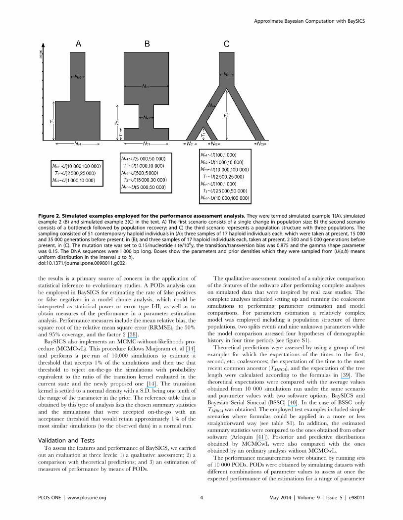
Figure 2. Simulated examples employed for the performance assessment analysis. They were termed simulated example 1(A), simulatedexample 2 (B) and simulated example 3(C) in the text. A) The first scenario consists of a single change in population size; B) the second scenarioconsists of a bottleneck followed by population recovery; and C) the third scenario represents a population structure with three populations. Thesampling consisted of 51 contemporary haploid individuals in (A); three samples of 17 haploid individuals each, which were taken at present, 15 000and 35 000 generations before present, in (B); and three samples of 17 haploid individuals each, taken at present, 2 500 and 5 000 generations beforepresent, in (C). The mutation rate was set to 0.15/nucleotide site/106y, the transition/transversion bias was 0.875 and the gamma shape parameterwas 0.15. The DNA sequences were l 000 bp long. Boxes show the parameters and prior densities which they were sampled from (U(a,b) meansuniform distribution in the interval a to b).doi:10.1371/journal.pone.0098011.g002

Approximate Bayesian Computation with BaySICS

PLOS ONE | www.plosone.org 4 May 2014 | Volume 9 | Issue 5 | e98011

values instead of a single combination of values. Each one of those

10 000 PODs were employed to use their parameters as the real

values and their summary statistics as the observed values for

which a parameter estimation by ABC was performed. Then, the

mean relative bias, the square root of the mean square error

(RRMSE), the 50% and 95% coverage, and the factor 2 were

calculated upon the 10 000 iterations (PODs). Notice that the

interpretation of some performance measures, such as RRMSE is

slightly different when obtained from PODs with different (real)

parameter values, than if the 10 000 PODs were obtained with the

same parameter values; however, the interpretation is still useful as

the procedure can be seen as an integration over the parametric

space of the simulated parameter values and the obtained

performance measures are thus the statistical expectation of those

measures. In this way, we can assess the performance of the

parameters estimation over a parametric space, instead of a single

combination of values, for a more general interpretation. Two

groups of performance measures were obtained, one using the

mode of the posterior distributions inferred from the accepted

sample as the estimator of the parameter, and one using the

median of the same distribution. Three sets of PODs were carried

out, each for a different scenario, with a different number of

parameters and complexity (figure 2): the first scenario contained

only one statistical group, five summary statistics and three

unknown parameters. The second example contained 19 summary

statistics from three statistical groups and had five unknown

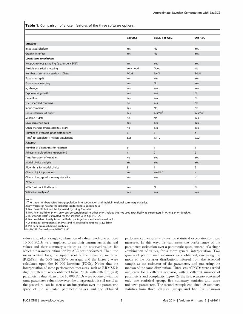
Table 1. Comparison of chosen features of the three software options.

BaySICS BSSC + R-ABC DIYABC

Interface

Integrated platform Yes No Yes

Graphic interface Yes No Yes

Coalescent Simulations

Heterochronous sampling (e.g. ancient DNA) Yes Yes Yes

Flexible statistical grouping Very good Good No

Number of summary statistics (DNA)1 7/2/4 7/4/1 8/5/0

Population split Yes Yes Yes

Populations merging Yes No Yes

Ne change Yes Yes Yes

Exponential growth Yes Yes No

Gene flow Yes Yes No

User specified formulas No Yes No

Input commands2 Yes No No

Cross reference of priors Yes Yes/No3 Yes/No4

Multilocus data No No Yes

DNA sequence data Yes Yes Yes

Other markers (microsatellites, SNP’s) No Yes Yes

Number of available prior distributions 6 5 4

Time5 to complete 1 million simulations 3.06 13.10 2.22

Analysis

Number of algorithms for rejection 2 1 1

Adjustment algorithms (regression) 1 2 2

Transformation of variables No Yes Yes

Model choice analysis Yes Yes Yes

Algorithms for model choice 2 1 2

Charts of joint posteriors Yes Yes/No6 -

Charts of accepted summary statistics Yes Yes -7

Others

MCMC without likelihoods Yes No No

Validation analyses8 Yes Yes Yes

Notes:1.The three numbers refer: intra-population, inter-population and multidimensional sum-mary statistics.2.Key words for having the program performing a specific task.3. Not possible but can be bypassed by using formulas.4. Not fully available: priors only can be conditioned to other priors values but not used specifically as parameters in other‘s prior densities.5. In seconds 6103; estimated for the scenario A in figure S1 A.6. Not available directly from the R-abc package but can be obtained in R.7. A principal components analysis and its respective graphic is available.8. PODs or cross-validation analyses.doi:10.1371/journal.pone.0098011.t001

Approximate Bayesian Computation with BaySICS

PLOS ONE | www.plosone.org 5 May 2014 | Volume 9 | Issue 5 | e98011

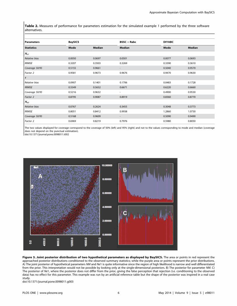
Table 2. Measures of performance for parameters estimation for the simulated example 1 performed by the three softwarealternatives.

Parameters BaySICS BSSC + Rabc DIYABC

Statistics Mode Median Median Mode Median

Ne1

Relative bias 0.0050 0.0697 0.0501 0.0077 0.0693

RRMSE 0.3207 0.3503 0.3269 0.3390 0.3610

Coverage 50/95 0.5155 0.9661 - 0.5040 0.9570

Factor 2 0.9581 0.9673 0.9676 0.9470 0.9630

t

Relative bias 0.0907 0.1401 0.1706 0.0483 0.1728

RRMSE 0.5549 0.5652 0.6671 0.6220 0.6660

Coverage 50/95 0.5216 0.9632 - 0.4900 0.9530

Factor 2 0.8795 0.9087 0.8919 0.8360 0.8770

Ne2

Relative bias 0.0767 0.2624 0.3455 0.3048 0.3773

RRMSE 0.8051 0.8412 0.9938 1.2860 1.0730

Coverage 50/95 0.5168 0.9609 - 0.5090 0.9490

Factor 2 0.6969 0.8219 0.7976 0.5980 0.8050

The two values displayed for coverage correspond to the coverage of 50% (left) and 95% (right) and not to the values corresponding to mode and median (coveragedoes not depend on the punctual estimation).doi:10.1371/journal.pone.0098011.t002

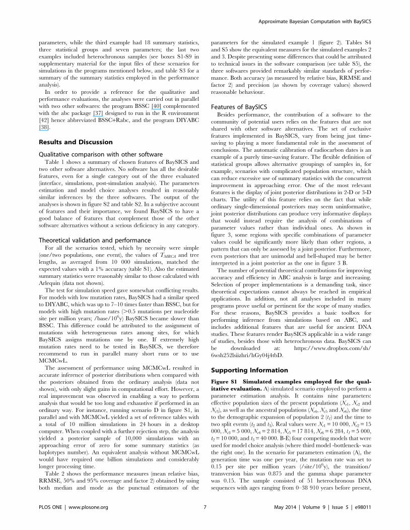
Figure 3. Joint posterior distribution of two hypothetical parameters as displayed by BaySICS. The area or points in red represent theapproached posterior distributions conditioned to the observed summary statistics; while the purple area or points represent the prior distributions.A) The joint posterior of hypothetical parameters NM and Ne1 is quite informative since the region of high likelihood is narrow and well differentiatedfrom the prior. This interpretation would not be possible by looking only at the single-dimensional posteriors. B) The posterior for parameter NM. C)The posterior of Ne1, where the posterior does not differ from the prior, giving the false perception that rejection (i.e. conditioning to the observeddata) has no effect for this parameter. This example was run by an artificial reference table but the shape of the posterior was inspired in a real casestudy.doi:10.1371/journal.pone.0098011.g003

Approximate Bayesian Computation with BaySICS

PLOS ONE | www.plosone.org 6 May 2014 | Volume 9 | Issue 5 | e98011

parameters, while the third example had 18 summary statistics,

three statistical groups and seven parameters; the last two

examples included heterochronous samples (see boxes S1-S9 in

supplementary material for the input files of these scenarios for

simulations in the programs mentioned below, and table S3 for a

summary of the summary statistics employed in the performance

analysis).

In order to provide a reference for the qualitative and

performance evaluations, the analyses were carried out in parallel

with two other softwares: the program BSSC [40] complemented

with the abc package [37] designed to run in the R environment

[42] hence abbreviated BSSC+Rabc, and the program DIYABC

[38].

Results and Discussion

Qualitative comparison with other softwareTable 1 shows a summary of chosen features of BaySICS and

two other software alternatives. No software has all the desirable

features, even for a single category out of the three evaluated

(interface, simulations, post-simulation analysis). The parameters

estimation and model choice analyses resulted in reasonably

similar inferences by the three softwares. The output of the

analyses is shown in figure S2 and table S2. In a subjective account

of features and their importance, we found BaySICS to have a

good balance of features that complement those of the other

software alternatives without a serious deficiency in any category.

Theoretical validation and performanceFor all the scenarios tested, which by necessity were simple

(one/two populations, one event), the values of TMRCA and tree

lengths, as averaged from 10 000 simulations, matched the

expected values with a 1% accuracy (table S1). Also the estimated

summary statistics were reasonably similar to those calculated with

Arlequin (data not shown).

The test for simulation speed gave somewhat conflicting results.

For models with low mutation rates, BaySICS had a similar speed

to DIYABC, which was up to 7–10 times faster than BSSC, but for

models with high mutation rates (.0.5 mutations per nucleotide

site per million years; /base/106y) BaySICS became slower than

BSSC. This difference could be attributed to the assignment of

mutations with heterogeneous rates among sites, for which

BaySICS assigns mutations one by one. If extremely high

mutation rates need to be tested in BaySICS, we therefore

recommend to run in parallel many short runs or to use

MCMCwL.

The assessment of performance using MCMCwL resulted in

accurate inference of posterior distributions when compared with

the posteriors obtained from the ordinary analysis (data not

shown), with only slight gains in computational effort. However, a

real improvement was observed in enabling a way to perform

analysis that would be too long and exhaustive if performed in an

ordinary way. For instance, running scenario D in figure S1, in

parallel and with MCMCwL yielded a set of reference tables with

a total of 10 million simulations in 24 hours in a desktop

computer. When coupled with a further rejection step, the analysis

yielded a posterior sample of 10,000 simulations with an

approaching error of zero for some summary statistics (as

haplotypes number). An equivalent analysis without MCMCwL

would have required one billion simulations and considerably

longer processing time.

Table 2 shows the performance measures (mean relative bias,

RRMSE, 50% and 95% coverage and factor 2) obtained by using

both median and mode as the punctual estimators of the

parameters for the simulated example 1 (figure 2). Tables S4

and S5 show the equivalent measures for the simulated examples 2

and 3. Despite presenting some differences that could be attributed

to technical issues in the software comparison (see table S5), the

three softwares provided remarkably similar standards of perfor-

mance. Both accuracy (as measured by relative bias, RRMSE and

factor 2) and precision (as shown by coverage values) showed

reasonable behaviour.

Features of BaySICSBesides performance, the contribution of a software to the

community of potential users relies on the features that are not

shared with other software alternatives. The set of exclusive

features implemented in BaySICS, vary from being just time-

saving to playing a more fundamental role in the assessment of

conclusions. The automatic calibration of radiocarbon dates is an

example of a purely time-saving feature. The flexible definition of

statistical groups allows alternative groupings of samples in, for

example, scenarios with complicated population structure, which

can reduce excessive use of summary statistics with the concurrent

improvement in approaching error. One of the most relevant

features is the display of joint posterior distributions in 2-D or 3-D

charts. The utility of this feature relies on the fact that while

ordinary single-dimensional posteriors may seem uninformative,

joint posterior distributions can produce very informative displays

that would instead require the analysis of combinations of

parameter values rather than individual ones. As shown in

figure 3, some regions with specific combinations of parameter

values could be significantly more likely than other regions, a

pattern that can only be assessed by a joint posterior. Furthermore,

even posteriors that are unimodal and bell-shaped may be better

interpreted in a joint posterior as the one in figure 3 B.

The number of potential theoretical contributions for improving

accuracy and efficiency in ABC analysis is large and increasing.

Selection of proper implementations is a demanding task, since

theoretical expectations cannot always be reached in empirical

applications. In addition, not all analyses included in many

programs prove useful or pertinent for the scope of many studies.

For these reasons, BaySICS provides a basic toolbox for

performing inference from simulations based on ABC, and

includes additional features that are useful for ancient DNA

studies. These features render BaySICS applicable in a wide range

of studies, besides those with heterochronous data. BaySICS can

be downloaded at: https://www.dropbox.com/sh/

6wsh252lsiizhri/hGy04j4tbD.

Supporting Information

Figure S1 Simulated examples employed for the qual-itative evaluation. A) simulated scenario employed to perform a

parameter estimation analysis. It contains nine parameters:

effective population sizes of the present populations (Ne1, Ne2 and

Ne3), as well as the ancestral populations (Ne4, Ne5 and Ne6), the time

to the demographic expansion of population 2 (t1) and the time to

two split events (t2 and t3). Real values were Ne1 = 10 000, Ne2 = 15

000, Ne3 = 5 000, Ne4 = 2 814, Ne5 = 17 814, Ne6 = 6 284, t1 = 5 000,

t2 = 10 000, and t3 = 40 000. B-E) four competing models that were

used for model choice analysis (where third model -bottleneck- was

the right one). In the scenario for parameters estimation (A), the

generation time was one per year, the mutation rate was set to

0.15 per site per million years (/site/106y), the transition/

transversion bias was 0.875 and the gamma shape parameter

was 0.15. The sample consisted of 51 heterochronous DNA

sequences with ages ranging from 0–38 910 years before present,

Approximate Bayesian Computation with BaySICS

PLOS ONE | www.plosone.org 7 May 2014 | Volume 9 | Issue 5 | e98011

and DNA sequences were 1 000 bp long. In the scenarios for

model choice (B-E) the generation time was 15 years, the mutation

rate was set to 0.247/site/106y, the transition/transversion bias

was 0.9798 and the gamma shape parameter was 0.05. The

sample consisted of 59 heterochronous DNA sequences with ages

ranging from 3 685 to 61 600 years before present. Analyzed

sequences were 741 bp long. Both analyses were inspired by real

data from case studies of ancient DNA.

(DOCX)

Figure S2 Posterior distributions of parameters esti-mated from the simulated data with three softwareoptions. Parameter names correspond to the ones in figure S1A.

Vertical scales represent probability but their interpretation is

relative so they were removed. Prior distributions are indicated as

grey dotted lines in charts from BSSC+Rabc and BaySICS and a

red line in DIYABC. The red curve indicates the posterior inferred

from linear regression while the black curve indicates the posterior

inferred from simple rejection in BSSC+Rabc. Small colorful

graphs are charts obtained in BaySICS with the options

‘histogram’ and ‘color informative’. Vertical dotted lines in purple

represent the real value. Note that this charts are not intended for

any performance assesment but only to make a qualitative

comparison of the programs’ output. Charts were distorted to

match their horizontal scales.

(DOCX)

Table S1 Expected and observed mean heights and lengths of

the coalescent trees for 10 test examples. The expected values for

the time to the most recent common ancestor (TMRCA) and tree

length (L) were obtained by formulas (theoretical) while the

observed ones were obtained by averaging over 10 000 simulations

that were performed with the programs BaySICS and Bayesian

Serial Simcoal (in the case of BSSC, only TMRCA). The test

scenarios corresponded to: 1–3) consisted of a single population

with a single sample consisting of contemporary samples and no

demographic events; 4–6) consisted of a single population with

samples taken at two times, one at generation zero and one at the

generation T indicated in the parameters column. In addition, the

population was subject to a sudden change of effective population

size going from size Ne1 to size Ne2. The time (in generations) of this

change coincided exactly with the time of sampling of the older

sample; 7–10) consisted of two populations with sizes Ne1 and Ne2

that originated from a split event that happened T generations ago

from an ancestral population with size Ne3. Two contemporary

samples were taken, one from each present population. For

examples 4–10, the theoretical expectation was obtained by

adding the expected lengths of each population sub-tree or each

sub-tree obtained from one contemporary subsample plus the

length of the lineages between the local MRCA and the next

event. Shown examples correspond only to a subset of the

examples analyzed. Additional tests involved different sample sizes

and parameter values as well as times to coalescent events other

than the MRCA. Notice that tests for different values of Ne are

somehow redundant since L and TMRCA only depend on Ne as a

scaling factor; unless heterochronous samples or demographic

events are involved.

(DOCX)

Table S2 Bayes factors among all pairwise comparisons of the

models tested in the model comparison analysis. They correspond

to scenarios B-E of figure S1. The rows in bold indicate the model

that obtained the highest support. Notice that this is just an essay

for a qualitative evaluation of the differences among programs and

not a test of performance.

(DOCX)

Table S3 Summary statistics employed for the performance test

of parameters estimation analysis. Abbreviations of the summary

statistics mean: HapTypesX: number of haplotypes in statistical

group X; PrivHapsX: number of private haplotypes in statistical

group X; SegSitesX: number of segregating sites in statistical group

X; PrivSegX: number of private segregating sites in statistical group

X; NucDiverX: nucleotide diversity in statistical group X; PairDiffsX:

average number of pairwise differences in statistical group X;

GenDiverX: gene diversity in statistical group X; VarPairD: variance

of pairwise differences; PairDiffsXvsY: average number of pairwise

differences between statistical group X and statistical group Y;

FstXvsY: FST between statistical groups X and Y. Since nucleotide

and average number of pairwise differences carry practically the

same information (NucDiver = PairDiffs/n; n = number of nucle-

otides), they are set in the same cell. Since the sets of summary

statistics available for each program were different, a set that

differed at minimum were chosen; the rationale was that using

identical sets of summary statistics would be pointless since the

differences among programs include the set of summary statistics

they have implemented.

(DOCX)

Table S4 Measures of performance for parameters estimation

for the simulated example 2. The two values displayed for

coverage correspond to the coverage of 50% (left) and 95% (right)

and not to the values corresponding to mode and median

(coverage does not depend of the punctual estimation).

(DOCX)

Table S5 Measures of performance for parameters estimation

for the simulated example 3. The two values displayed for

coverage correspond to the coverage of 50% (left) and 95% (right)

and not to the values corresponding to mode and median,

(coverage does not depend of the punctual estimation). In both

simulated example 2 and simulated example 3, the estimates

obtained with DIYABC presented important inconsistencies when

the number of iterations (PODs) varied: the ones obtained for 10

000 iterations were one order of magnitude larger than those

obtained with 1 000 iterations. In addition, most of the values are

much more similar between BSSC+Rabc and BaySICS. Those

facts could be indicative of a numerical issue of the type of

‘‘catastrophic cancelation’’. So the true performance measures for

DIYABC clearly should be much better for those parameters.

(DOCX)

Box S1 Input file for simulation of the SimulatedExample 1 in BaySICS.

(DOCX)

Box S2 Input file for simulation of the SimulatedExample 2 in BaySICS.

(DOCX)

Box S3 Input file for simulation of the SimulatedExample 3 in BaySICS.

(DOCX)

Box S4 Input file for simulation of the SimulatedExample 1 in BSSC.

(DOCX)

Box S5 Input file for simulation of the SimulatedExample 2 in BSSC.

(DOCX)

Box S6 Input file for simulation of the SimulatedExample 3 in BSSC.

(DOCX)

Approximate Bayesian Computation with BaySICS

PLOS ONE | www.plosone.org 8 May 2014 | Volume 9 | Issue 5 | e98011

Box S7 Header file for simulation of the SimulatedExample 1 in DIYABC.(DOCX)

Box S8 Header file for simulation of the SimulatedExample 2 in DIYABC.(DOCX)

Box S9 Header file for simulation of the SimulatedExample 3 in DIYABC.(DOCX)

Acknowledgments

We thank Mattias Jakobsson and Karolina Doan for their feedback

regarding the program. We also thank an anonymous reviewer for his/her

constructive comments.

Author Contributions

Conceived and designed the experiments: ES EP. Performed the

experiments: ES EP. Analyzed the data: ES EP. Wrote the paper: ES

LD. Designed and programed the presented software: ES.

References

1. Hudson RR, Kaplan NL (1987) Applications of the Coalescent Process toProblems in Population-Genetics. Environ Health Persp 75: 126–127.

2. Beaumont MA, Zhang W, Balding DJ (2002) Approximate Bayesiancomputation in population genetics. Genetics 162(4): 2025–2035.

3. Nielsen R, Paul JS, Albrechtsen A, Song YS (2011) Genotype and SNP calling

from next-generation sequencing data. Nat Rev Genet 12(6): 443–451.4. Kingman JFC (1982) The coalescent. Stoch Proc Appl 13: 235–248.

5. Shoemaker JS, Painter IS, Weir BS (1999) Bayesian statistics in genetics - a guidefor the uninitiated. Trends in Genetics 15(9): 354–358.

6. Beaumont MA, Rannala B (2004) The Bayesian revolution in genetics. Nat RevGenet 5(4): 251–261.

7. Turner BM, Van Zandt T (2012) A tutorial on approximate Bayesian

computation. J Math Psychol 56(2): 69–85.8. Morozova O, Marra MA (2008) Applications of next-generation sequencing

technologies in functional genomics. Genomics 92(5): 255–264.9. Green RE, Krause J, Briggs AW, Maricic T, Stenzel U, et al. (2010) A Draft

Sequence of the Neandertal Genome. Science 328(5979): 710–722.

10. Van Tuinen M, Ramakrishnan U, Hadly EA (2004) Studying the effect ofenvironmental change on biotic evolution: past genetic contributions, current

work and future directions. Philos T Roy Soc A 362(1825): 2795–2820.11. Ramakrishnan U, Hadly EA (2009) Using phylochronology to reveal cryptic

population histories: review and synthesis of 29 ancient DNA studies. Mol Ecol

18(7): 1310–1330.12. Beaumont MA (2010) Approximate Bayesian Computation in Evolution and

Ecology. Annu Rev Ecol Evol S 41: 379–406.13. Csillery K, Blum MGB, Gaggiotti OE, Francois O (2010) Approximate Bayesian

Computation (ABC) in practice. Trends Ecol Evol 25(7): 410–418.14. Marjoram P, Molitor J, Plagnol V, Tavare S (2003) Markov chain Monte Carlo

without likelihoods. P Natl Acad Sci USA 100(26): 15324–15328.

15. Fagundes NJR, Ray N, Beaumont M, Neuenschwander S, Salzano FM, et al.(2007) Statistical evaluation of alternative models of human evolution. P Natl

Acad Sci USA 104(45): 17614–17619.16. Sjodin P, Sjostrand AE, Jakobsson M, Blum MGB (2012) Resequencing Data

Provide No Evidence for a Human Bottleneck in Africa during the Penultimate

Glacial Period. Mol Biol Evol 29(7): 1851–1860.17. Shriner D, Liu Y, Nickle DC, Mullins JI (2006) Evolution of intrahost HIV-1

genetic diversity during chronic infection. Evolution 60(6): 1165–1176.18. Tanaka MM, Francis AR, Luciani F, Sisson SA (2006) Using approximate

Bayesian computation to estimate tuberculosis transmission parameters fromgenotype data. Genetics 173(3): 1511–1520.

19. Pritchard JK, Seielstad MT, Perez-Lezaun A, Feldman MW (1999) Population

growth of human Y chromosomes: A study of Y chromosome microsatellites.Mol Biol Evol, 16(12): 1791–1798.

20. Hamilton G, Currat M, Ray N, Heckel G, Beaumont M, et al. (2005) Bayesianestimation of recent migration rates after a spatial expansion. Genetics 170(1):

409–417.

21. Jensen JD, Thornton KR, Andolfatto P (2008) An Approximate BayesianEstimator Suggests Strong, Recurrent Selective Sweeps in Drosophila. Plos

Genet 4(9): e1000198. doi:10.1371/journal.pgen.1000198.22. Sousa VC, Fritz M, Beaumont MA, Chikhi L (2009) Approximate Bayesian

computation without summary statistics: the case of admixture. Genetics 181(4):1507–1519.

23. Excoffier L, Novembre J, Schneider S (2000) SIMCOAL: A general coalescent

program for the simulation of molecular data in interconnected populations witharbitrary demography. J Hered 91(6): 506–509.

24. Chan YL, Hadly EA (2011) Genetic variation over 10 000 years in Ctenomys:

comparative phylochronology provides a temporal perspective on rarity,

environmental change and demography. Mol Ecol 20(22): 4592–4605.

25. Mellows A, Barnett R, Dalen L, Sandoval-Castellanos E, Linderholm A, et al.

(2012) The impact of past climate change on genetic variation and population

connectivity in the Icelandic arctic fox. Proc R Soc B 279: 4568–4573.

26. Nystrom V, Humphrey J, Skoglund P, McKeown NJ, Vartanyan S, et al. (2012)

Microsatellite genotyping reveals end-Pleistocene decline in mammoth autoso-

mal genetic variation. Mol Ecol 21(14): 3391–3402.

27. Bertorelle G, Benazzo A, Mona S (2010) ABC as a flexible framework to

estimate demography over space and time: some cons, many pros. Mol Ecol

19(13): 2609–2625.

28. Robert CP, Cornuet JM, Marin JM, Pillai NS (2011) Lack of confidence in

approximate Bayesian computation model choice. P Natl Acad Sci USA 108(37):

15112–15117.

29. Ratmann O, Andrieu C, Wiuf C, Richardson S (2009) Model criticism based on

likelihood-free inference, with an application to protein network evolution. P Natl

Acad Sci USA 106(26): 10576–10581.

30. Sisson SA, Fan Y, Tanaka MM (2007) Sequential Monte Carlo without

likelihoods. P Natl Acad Sci USA 104(6): 1760–1765.

31. Wegmann D, Leuenberger C, Excoffier L (2009) Efficient approximate Bayesian

computation coupled with Markov chain Monte Carlo without likelihood.

Genetics 182(4): 1207–1218.

32. Blum MGB, Francois O (2010) Non-linear regression models for Approximate

Bayesian Computation. Stat Comput 20(1): 63–73.

33. Leuenberger C, Wegmann D (2010) Bayesian Computation and Model

Selection Without Likelihoods. Genetics 184(1): 243–252.

34. Liepe J, Barnes C, Cule E, Erguler K, Kirk P, et al. (2010) ABC-SysBio-

approximate Bayesian computation in Python with GPU support. Bioinfor-

matics 26(14): 1797–1799.

35. Lopes JS, Beaumont MA (2010) ABC: a useful Bayesian tool for the analysis of

population data. Infect Genet Evol 10(6): 826–833.

36. Wegmann D, Leuenberger C, Neuenschwander S, Excoffier L (2010) ABCtool-

box: a versatile toolkit for approximate Bayesian computations. BMC

Bioinformatics 11: 116.

37. Csillery K, Francois O, Blum MGB (2012) abc: an R package for approximate

Bayesian computation (ABC). Methods Ecol Evol 3(3): 475–479.

38. Cornuet JM, Pudlo P, Veyssier J, Dehne-Garcia A, Gautier M, et al. (2014)

DIYABC v2.0: a software to make approximate Bayesian computation

inferences about population history using single nucleotide polymorphism,

DNA sequence and microsatellite data. Bioinformatics 30(8): 1187–1189.

39. Hein J, Schierup MH, Wiuf C (2010) Gene Genealogies, Variation and

Evolution: A Primer in Coalescent Theory. Oxford: Oxford University Press.

276 p.

40. Anderson CNK, Ramakrishnan U, Chan YL, Hadly EA (2005) Serial SimCoal:

A population genetics model for data from multiple populations and points in

time. Bioinformatics 21(8): 1733–1734.

41. Excoffier L, Lischer HEL (2010) Arlequin suite ver 3.5: a new series of programs

to perform population genetics analyses under Linux and Windows. Mol Ecol

Resour 10: 564–567.

42. R Development Core Team (2008) R: A language and environment for

statistical computing. R. F. f. S. Computing, Vienna, Austria.

Approximate Bayesian Computation with BaySICS

PLOS ONE | www.plosone.org 9 May 2014 | Volume 9 | Issue 5 | e98011