Back Propagation and Other Differentiation Algorithmssrihari/CSE676/6.6 BackPropagation.pdf · – Backpropagation is an algorithm that computes the chain rule, with a specific order

Deep Learning Srihari

1

Back Propagation and Other Differentiation Algorithms

Sargur N. Srihari [email protected]


Topics (Deep Feedforward Networks)

•  Overview 1. Example: Learning XOR 2. Gradient-Based Learning 3. Hidden Units 4. Architecture Design 5. Backpropagation and Other Differentiation

Algorithms 6. Historical Notes

2


Topics in Backpropagation 1.  Overview 2.  Computational Graphs 3.  Chain Rule of Calculus 4.  Recursively applying the chain rule to obtain

backprop 5.  Backpropagation computation in fully-connected MLP 6.  Symbol-to-symbol derivatived 7.  General backpropagation 8.  Ex: backpropagation for MLP training 9.  Complications 10. Differentiation outside the deep learning community 11. Higher-order derivatives

3


Overview of Backpropagation

4

Deep Learning Srihari Forward Propagation

•  Producing an output from input – When we use a Feed-Forward Network to accept

an input x and produce an output information x propagates to hidden units at each layer and finally produces

– This is called forward propagation •  During training (quality of result is evaluated):

–  forward propagation can continue onward – until it produces scalar cost J (θ) over N training

samples (xn,yn)

5

y

y


Equations for Forward Propagation

6

First layer given by h(1)=g(1)(W(1)Tx + b(1)) Second layer is h(2)=g(2)(W(2)Th(2)+ b(2)), ….. Final output is =g(d)(W(d)Th(d)+ b(d))

Producing an output:

y

J(θ) = J

MLE+λ W

i,j(1)( )2

+ Wi,j(2)( )2

+ ....i,j∑

i,j∑⎛

⎝⎜⎜⎜⎜

⎞

⎠⎟⎟⎟⎟

J

MLE=

1N

|| y−yn||2

n=1

N

∑

During training, cost over n exemplars:


Back-Propagation Algorithm •  Often simply called backprop

– Allows information from the cost to flow back through network to compute gradient

•  Computing analytical expression for the gradient is straightforward – But numerically evaluating the gradient is

computationally expensive •  The backpropagation algorithm does this using

a simple and inexpensive procedure

7


Analytical Expression for Gradient

•  Sum-of-squares criterion over n samples

– Expression for gradient

•  Another way of saying the same with cost J(θ):

8

E(w)=12

wTφ(xn) -t

n{ }n=1

N

∑2

∇wE(w)= wTφ(x

n) - t

n{ }n=1

N

∑ φ(xn)

Jn(θ) =||θTx

n−y

n||2

∇θJn

(θ) = θT θ xn− y

n( ) = θTθxn−θT y

n


Backpropagation is not Learning •  Backpropagation often misunderstood as the

whole learning algorithm for multilayer networks –  It only refers to method of computing gradient

•  Another algorithm, e.g., SGD, is used to perform learning using this gradient – Learning is updating weights using gradient:

•  Backpropagation is also misunderstood to being specific to multilayer neural networks –  It can be used to compute derivatives for any

function (or report that the derivative is undefined) 9

w (τ+1) =w (τ ) −η∇Jn (θ )


Importance of Backpropagation

•  Backprop is a technique for computing derivatives quickly –  It is the key algorithm that makes training deep

models computationally tractable – For modern neural networks it can make training

gradient descent 10 million times faster relative to naiive implementation

•  It is the difference between a model that takes a week to train instead of 200,000 years

10

Deep Learning Srihari Computing gradient for arbitrary function

•  Arbitrary function f(x,y) – x : variables for which derivatives are desired –  y is an additional set of variables that are inputs to

the function but whose derivatives are not required •  Gradient required is of cost wrt parameters, •  Backprop is also useful for other ML tasks

–  Those that need derivatives, as part of learning process or to analyze a learned model

–  To compute Jacobian of a function f with multiple outputs

•  We restrict to case where f has a single output

∇x f (x,y)

∇θJ(θ)


Computational Graphs

12

Deep Learning Srihari Computational Graphs

•  To describe backpropagation use precise computational graph language – Each node is either

•  A variable –  Scalar, vector, matrix, tensor, or other type

•  Or an Operation –  Simple function of one or more variables –  Functions more complex than operations are obtained by

composing operations

–  If variable y is computed by applying operation to variable x then draw directed edge from x to y


Ex: Computational Graph of xy

(a)  Compute z = xy

14


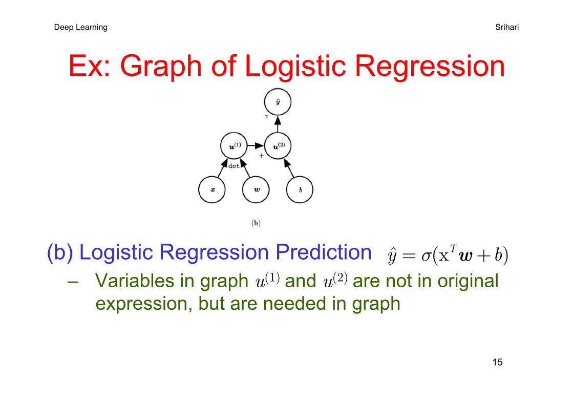
Ex: Graph of Logistic Regression

(b) Logistic Regression Prediction –  Variables in graph u(1) and u(2) are not in original

expression, but are needed in graph

15

y = σ(xTw +b)


Ex: Graph for ReLU

(c) Compute expression H=max{0,XW+b} – Computes a design matrix of Rectified linear unit

activations H given design matrix of minibatch of inputs X

16


Ex: Two operations on input

(d) Perform more than one operation to a variable

Weights w are used in two operations:

•  to make prediction and •  the weight decay penalty

17

y

λ w

i2

i∑


Chain Rule of Calculus

18


Calculus’ Chain Rule for Scalars •  Formula for computing derivatives of functions

formed by composing other functions whose derivatives are known – Backpropagation is an algorithm that computes the

chain rule, with a specific order of operations that is highly efficient

•  Let x be a real number •  Let f and g be functions mapping from a real number to a

real number •  If y=g(x) and z=f (g(x))=f (y)

•  Then the chain rule states that 19

dzdx

= dzdy

⋅ dydx


•  Suppose g maps from Rm to Rn and f from Rn to R

•  If y=g(x) and z=f (y) then •  In vector notation this is

•  where is the n x m Jacobian matrix of g

•  Thus gradient of z wrt x is product of: •  Jacobian matrix and gradient vector •  Backprop algorithm consists of performing

Jacobian-gradient product for each step of graph

g

x

y

Generalizing Chain Rule to Vectors x ∈Rm,y ∈Rn

∂z∂x

i

=∂z∂y

j

⋅∂y

j

∂xj∑

∇xz=

∂y∂x

⎛⎝⎜

⎞⎠⎟

T

∇yz

∂y∂x

⎛⎝⎜

⎞⎠⎟

∂y∂x

∇yz


Generalizing Chain Rule to Tensors

•  Backpropagation is usually applied to tensors with arbitrary dimensionality

•  This is exactly the same as with vectors – Only difference is how numbers are arranged in a

grid to form a tensor •  We could flatten each tensor into a vector, compute a

vector-valued gradient and reshape it back to a tensor

•  In this view backpropagation is still multiplying Jacobians by gradients

21 ∇xz=

∂y∂x

⎛⎝⎜

⎞⎠⎟

T

∇yz

Deep Learning Srihari Chain Rule for tensors

•  To denote gradient of value z wrt a tensor X we write as if X were a vector

•  For 3-D tensor, X has three coordinates – We can abstract this away by using a single

variable i to represent complete tuple of indices •  For all possible tuples i gives

•  Exactly same as how for all possible indices i into a vector, gives

•  Chain rule for tensors –  If Y=g (X) and z=f (Y) then

22

∇Xz

∇

Xz( )

i

∂z∂X

i

∇

X(z)=

j∑ ∇

XY

j( ) ∂z∂Yj

∇

Xz( )

i

∂z∂X

i

g

x

y


Recursively applying the chain rule to obtain backprop

23


Backprop is Recursive Chain Rule •  Backprop is obtained by recursively applying

the chain rule •  Using chain rule it is straightforward to write

expression for gradient of a scalar wrt any node in graph for producing that scalar

•  However, evaluating that expression on a computer has some extra considerations – E.g., many subexpressions may be repeated

several times within overall expression •  Whether to store subexpressions or recompute them

24

Deep Learning Srihari Example of repeated subexpressions

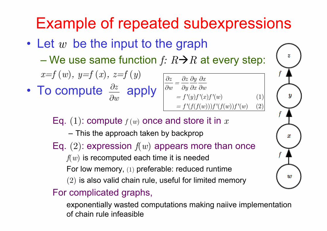
•  Let w be the input to the graph – We use same function f: RàR at every step: x=f (w), y=f (x), z=f (y)

•  To compute apply Eq. (1): compute f (w) once and store it in x

–  This the approach taken by backprop

Eq. (2): expression f(w) appears more than once f(w) is recomputed each time it is needed For low memory, (1) preferable: reduced runtime (2) is also valid chain rule, useful for limited memory

For complicated graphs, exponentially wasted computations making naiive implementation of chain rule infeasible

∂z∂w

=∂z∂y∂y∂x∂x∂w

= f '(y)f '(x)f '(w) (1) = f '(f (f (w)))f '(f (w))f '(w) (2)

∂z∂w


Simplified Backprop Algorithm •  Version that directly computes actual gradient

–  In the order it will actually be done according to recursive application of chain rule

•  Algorithm Simplified Backprop along with associated •  Forward Propagation

•  Could either directly perform these operations –  or view algorithm as symbolic specification of

computational graph for computing the back-prop •  This formulation does not make specific

– Manipulation and construction of symbolic graph that performs gradient computation


Computing a single scalar •  Consider computational graph of how to

compute scalar u(n) – say loss on a training example

•  We want gradient of this scalar u(n) wrt ni input nodes u(1),..u(ni)

•  i.e., we wish to compute for all i =1,..,ni

•  In application of backprop to computing gradients for gradient descent over parameters –  u(n) will be cost associated with an example or a

minibatch, while –  u(1),..u(ni) correspond to model parameters

∂u(n)

∂ui

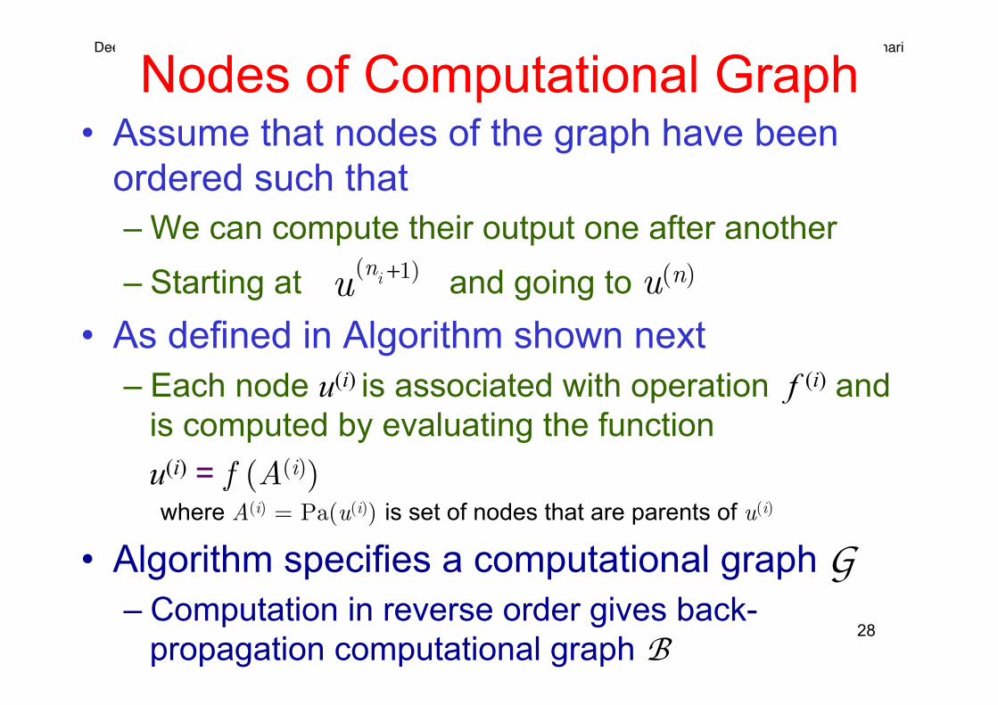
Deep Learning Srihari Nodes of Computational Graph

•  Assume that nodes of the graph have been ordered such that – We can compute their output one after another – Starting at and going to u(n)

•  As defined in Algorithm shown next – Each node u(i) is associated with operation f (i) and

is computed by evaluating the function u(i) = f (A(i))

where A(i) = Pa(u(i)) is set of nodes that are parents of u(i)

•  Algorithm specifies a computational graph G– Computation in reverse order gives back-

propagation computational graph B

28

u(ni +1)

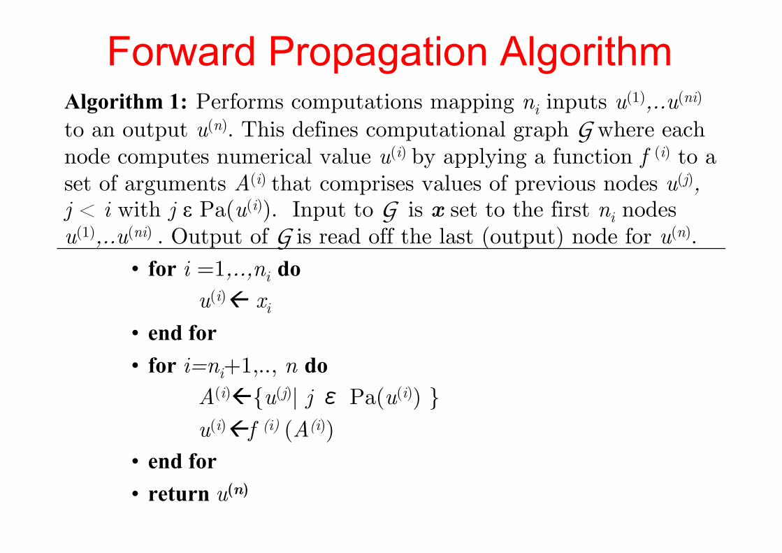
Deep Learning Srihari Forward Propagation Algorithm Algorithm 1: Performs computations mapping ni inputs u(1),..u(ni) to an output u(n). This defines computational graph G where each node computes numerical value u(i) by applying a function f (i) to a set of arguments A(i) that comprises values of previous nodes u(j), j < i with j ε Pa(u(i)). Input to G is x set to the first ni nodes u(1),..u(ni) . Output of G is read off the last (output) node for u(n).

•  for i =1,..,ni do u(i)ß xi

•  end for •  for i=ni+1,.., n do A(i)ß{u(j)| j ε Pa(u(i)) } u(i)ßf (i) (A(i)) •  end for •  return u(n)


Computation in B

•  Proceeds exactly in reverse order of computation in G

•  Each node in B computes the derivative associated with the forward graph node u(i)

•  This is done using the chain rule wrt the scalar output u(n)

30

∂u(n)

∂ui

∂u(n)

∂u(j)=

∂u(n)

∂u(i)

∂u(i)

∂u(j)i:jÎPa u(i)( )∑


Preamble to Simplified Backprop

•  Objective is to compute derivatives of u(n) with respect to variables in the graph – Here all variables are scalars and we wish to

compute derivatives wrt – We wish to compute the derivatives wrt u(1),..u(ni)

•  Algorithm computes the derivatives of all nodes in the graph

31

Deep Learning Srihari Simplified Backprop Algorithm

32

•  Algorithm 2: For computing derivatives of u(n) wrt variables in G. All variables are scalars and we wish to compute derivatives wrt u(1),..u(ni) . We compute derivatives of all nodes in G.

•  Run forward propagation to obtain network activations •  Initialize grad-table, a data structure that will store derivatives that

have been computed, The entry grad-table [u(i)] will store the computed value of

1.  grad-table [u(n)] ß1 2.  for j=n-1 down to 1 do grad-table [u(j)] ß 3. endfor 4. return {[u(i)] |i=1,.., ni}

∂u(n)

∂ui

grad-table u(i )⎡⎣ ⎤⎦

i: j∈Pa u( i )( )∑ ∂u(i )

∂u( j )

Step2computes∂u(n)

∂u( j )= ∂u(n)

∂u(i )i: j∈Pa u( i )( )∑ ∂u(i )

∂u( j )


Computational Complexity

•  Computational cost is proportional to no. of edges in graph (same as for forward prop) – Each is a function of the parents of u(j) and u(i)

thus linking nodes of the forward graph to those added for B

•  Backpropagation thus avoids exponential explosion in repeated subexpressions – By simplifications on the computational graph

33

∂u(i)

∂u(j)


Generalization to Tensors

•  Backprop is designed to reduce the no. of common sub-expressions without regard to memory

•  It performs on the order of one Jacobian product per node in the graph

34


35

Backprop in fully connected MLP


Backprop in fully connected MLP

•  Consider specific graph associated with fully-connected multilayer perceptron

•  Algorithm discussed next shows forward propagation – Maps parameters to supervised loss

associated with a single training example (x,y) with the output when x is the input

36

L y , y( )

y

Deep Learning Srihari Forward Prop: deep nn & cost computation

37

•  Algorithm 3: The loss L(y,y depends on output and on the target y. To obtain total cost J the loss may be added to a regularizer Ω(θ) where θ contains all the parameters (weights and biases).Algorithm 4 computes gradients of J wrt parameters W and b. This demonstration uses only single input example x.

•  Require: Net depth l; Weight matrices W(i), i ε{1,..,l}; bias parameters b(i), i ε{1,..,l}; input x; target output y

1. h(0) = x 2.  for k =1 to l do a(k) = b(k)+W(k)h(k-1)

h(k)=f(a(k)) 3. end for 4.  = h(l)

J= + λΩ(θ)

L y,y( )

L y,y( )

y

y

Deep Learning Srihari Backward compute: deep NN of Algorithm 3

38

Algorithm 4: uses in addition to input x a target y. Yields gradients on activations a(k) for each layer starting from output layer to first hidden layer. From these gradients one can obtain gradient on parameters of each layer, Gradients can be used as part of SGD.

After forward computation compute gradient on output layer g ß for k= l , l -1,..1 do Convert gradient on layer’s output into a gradient into the pre- nonlinearity activation (elementwise multiply if f is elementwise) g ß Compute gradients on weights biases (incl. regularizn term) Propagate the gradients wrt the next lower-level hidden layer’s activations: gß end for

∇ y J =∇ yL( y , y)

∇a(k )J = g⊙ f ' a(k )( )

∇h(k−1)J =W (k )Tg

∇b(k )J = g+λ∇

b(k )Ω(θ ),∇

W (k ) J = gh(k−1)T +λ∇W (k )Ω(θ )


Symbol-to-Symbol Derivatives

•  Both algebraic expressions and computational graphs operate on symbols, or variables that do not have specific values

•  They are called symbolic representations •  When we actually use or train a neural network,

we must assign specific values for these symbols

•  We replace a symbolic input to the network with a specific numeric value – E.g., [2.5, 3.75, -1.8]T 39


Two approaches to backpropagation 1.  Symbol-to-number differentiation

– Take a computational graph and a set of numerical values for inputs to the graph

– Return a set of numerical values describing gradient at those input values

– Used by libraries: Torch and Caffe 2.  Symbol-to-symbol differentiation

– Take a computational graph – Add additional nodes to the graph that provide

a symbolic description of desired derivatives – Used by libraries: Theano and Tensorflow 40


Symbol-to-symbol Derivatives

41

•  To compute derivative using this approach, backpropagation does not need to ever access any actual numerical values –  Instead it adds nodes to a computational

graph describing how to compute the derivatives for any specific numerical values

– A generic graph evaluation engine can later compute derivatives for any specific numerical values


Ex: Symbol-to-symbol Derivatives

42

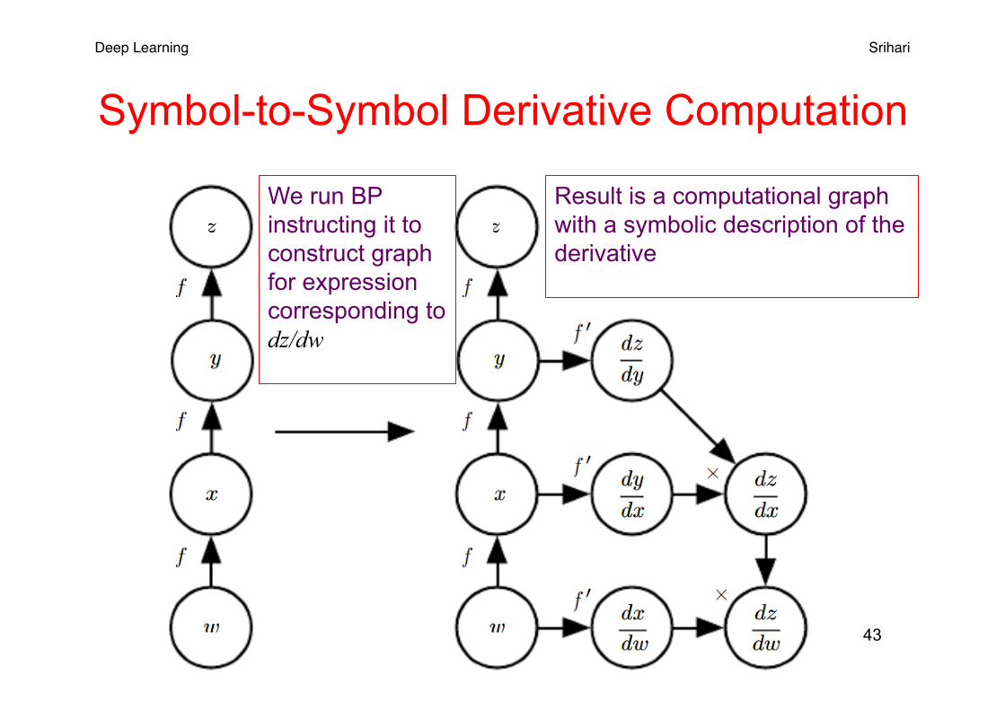
•  Begin with graph representing z=f ( f ( f (w)))


Symbol-to-Symbol Derivative Computation

43

Result is a computational graph with a symbolic description of the derivative

We run BP instructing it to construct graph for expression corresponding to dz/dw


Advantages of Approach

•  Derivatives are described in the same language as the original expression

•  Because the derivatives are just another computational graph, it is possible to run back-propagation again – Differentiating the derivatives – Yields higher-order derivatives

44

Deep Learning Srihari General Backpropagation

•  To compute gradient of scalar z wrt one of its ancestors x in the graph – Begin by observing that gradient wrt z is – Then compute gradient wrt each parent of z

by multiplying current gradient by Jacobian of: operation that produced z

– We continue multiplying by Jacobians traveling backwards until we reach x

– For any node that can be reached by going backwards from z through two or more paths sum the gradients from different paths at that node

dzdz

=1

g

x

y

∇xz=

∂y∂x

⎛⎝⎜

⎞⎠⎟

T

∇yz


Formal Notation for backprop

•  Each node in the graph G corresponds to a variable

•  Each variable is described by a tensor V – Tensors have any no. of dimensions – They subsume scalars, vectors and matrices

46


Each variable V is associated with the following subroutines:

•  get_operation (V) – Returns the operation that computes V

represented by the edges coming into V in G – Suppose we have a variable that is computed

by matrix multiplication C=AB •  Then get_operation (V) returns a pointer to an

instance of the corresponding C++ class

47


Other Subroutines of V

•  get_consumers (V, G) – Returns list of variables that are children of V

in the computational graph G•  get_inputs (V, G)

– Returns list of variables that are parents of V in the computational graph G

48


bprop operation

•  Each operation op is associated with a bprop operation •  bprop operation can compute a Jacobian vector

product as described by •  This is how the backpropagation algorithm can

achieve great generality – Each operation is responsible for knowing how to

backpropagate through the edges in the graph that it participates in

∇xz =

∂y∂x

⎛⎝⎜

⎞⎠⎟

T

∇ yz

Deep Learning Srihari Example of bprop

•  Suppose we have •  a variable computed by matrix multiplication C=AB –  the gradient of a scalar z wrt C is given by G

•  The matrix multiplication operation is responsible for two back propagation rules – One for each of its input arguments

•  If we call bprop to request the gradient wrt A given that the gradient on the output is G

–  Then bprop method of matrix multiplication must state that gradient wrt A is given by GBT

•  If we call bprop to request the gradient wrt B –  Then matrix operation is responsible for implementing the bprop

and specifying that the desired gradient is ATG

Deep Learning Srihari Inputs, outputs of bprop

•  Backprogation algorithm itself does not need to know any differentiation rules –  It only needs to call each operation’s bprop rules

with the right arguments •  Formally op.bprop (inputs X, G) must return

•  which is just an implementation of the chain rule

•  inputs is a list of inputs that are supplied to the operation, op.f is a math function that the operation implements,

• X is the input whose gradient we wish to compute, • G is the gradient on the output of the operation 51

∇xop.f(inputs)i( )

i∑ Gi

∇xz =

∂y∂x

⎛⎝⎜

⎞⎠⎟

T

∇ yz


Computing derivative of x2

•  Example: The mul operator is passed to two copies of x to compute x2

•  The ob.prop still returns x as derivative wrt to both inputs

•  Backpropagation will add both arguments together to obtain 2x

52


Software Implementations •  Usually provide both:

1.  Operations 2.  Their bprop methods

•  Users of software libraries are able to backpropagate through graphs built using common operations like – Matrix multiplication, exponents, logarithms, etc

•  To add a new operation to existing library must derive ob.prop method manually

53


Formal Backpropagation Algorithm

54

•  Algorithm 5: Outermost skeleton of backprop •  This portion does simple setup and cleanup work, Most of the

important work happens in the build_grad subroutine of Algorithm 6

•  Require: T, Target set of variables whose gradients must be computed

•  Require: G, the computational graph 1.  Let G’ be G pruned to contain only nodes that are

ancestors of z and descendants of nodes in T 2.  for V in T do build-grad (V,G , G’, grad-table)

endfor 4.  Return grad-table restricted to T

Deep Learning Srihari Inner Loop: build-grad

55

•  Algorithm 6: Innerloop subroutine build-grad(V,G,G’,grad-table) of the back-propagation algorithm, called by Algorithm 5

•  Require: V, Target set of variables whose gradients to be computed; G, the graph to modify; G’, the restriction of G to modify; grad-table,a data structure mapping nodes to their gradients

if V is in grad-table, then return grad-table [V] endif iß1 for C in get-customers(V,G’) do

opßget-operation(C) Dßbuild-grad(C,G,G’,grad-table) G(i)ßob.bprop(get-inputs(C,G’),V,D) ißi+1

endfor Gß ΣiG(i)

grad-table[V] = G

Insert G and the operations creating it into G Return G

Deep Learning Srihari Ex: backprop for MLP training

•  As an example, walk through back-propagation ealgorithm as it is used to train a multilayer perceptron

•  We use Minibatch stochastic gradient descent •  Backpropagation algorithm is used to compute

the gradient of the cost on a single minibatch •  We use a minibatch of examples from the

training set formatted as a design matrix X, and a vector of associated class labels y

56

Deep Learning Srihari Ex: details of MLP training

•  Network computes a layer hidden features H=max{0,XW(1)} – No biases in model

•  Graph language has relu to compute max{0,Z}

•  Prediction: log-probs(unnorm) over classes: HW(2)

•  Graph language includes cross-entropy operation – computes cross-entropy between targets y and

probability distribution defined by log probs – Resulting cross-entropy defines cost JMLE – We include a regularization term 57


Forward propagation graph

58

Total cost:


Computational Graph of Gradient •  It would be large and tedious for this

example •  One benefit of back-propagation algorithm

is that it can automatically generate gradients that would be straightforward but tedious manually for a software engineer to derive

59

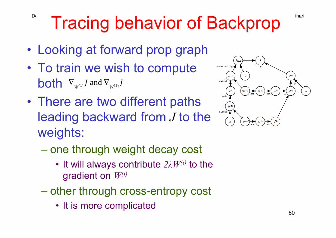
Deep Learning Srihari Tracing behavior of Backprop •  Looking at forward prop graph •  To train we wish to compute

both •  There are two different paths

leading backward from J to the weights: – one through weight decay cost

•  It will always contribute 2λW(i) to the gradient on W(i)

– other through cross-entropy cost •  It is more complicated

60

∇W (1) J and∇W (2) J

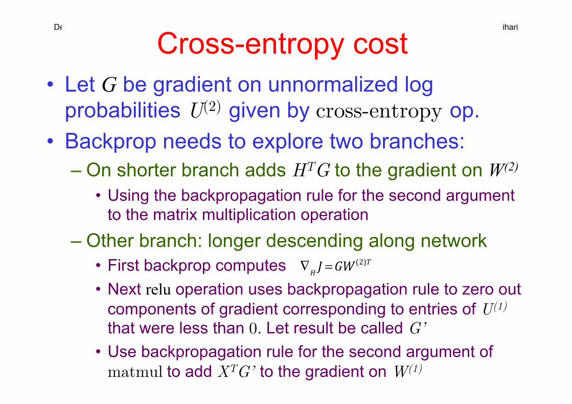
Deep Learning Srihari Cross-entropy cost

•  Let G be gradient on unnormalized log probabilities U(2) given by cross-entropy op.

•  Backprop needs to explore two branches: – On shorter branch adds HTG to the gradient on W(2)

•  Using the backpropagation rule for the second argument to the matrix multiplication operation

– Other branch: longer descending along network •  First backprop computes •  Next relu operation uses backpropagation rule to zero out

components of gradient corresponding to entries of U(1) that were less than 0. Let result be called G’

•  Use backpropagation rule for the second argument of matmul to add XTG’ to the gradient on W(1)

∇H J =GW(2)T


After Gradient Computation

•  It is the responsibility of SGD or other optimization algorithm to use gradients to update parameters

62

Back Propagation and Other Differentiation Algorithmssrihari/CSE676/6.6 BackPropagation.pdf · – Backpropagation is an algorithm that computes the chain rule, with a specific order

Documents